Political Insulation and Lobbying Tobias B¨ ohm * 02.04.2007 Abstract The aim of the present paper is to show how inefficient redistribution can occur in a dynamic menu auction lobbying game. I study a two period lobbying game in which the politician has the choice between an efficient lump sum transfer and an inefficient output subsidy. Since the output subsidy increases production and therefore capacity in an industry, future governments may be more willing to sustain the subsidy in order to avoid costs associated with capacity reduction. As this saves lobbying contributions in the future, the present government may have an incentive to collude with the interest group at the expense of future governments, and implement inefficient transfers. This effect is shown to be even more pronounced if the degree of competition between lobbies increases. JEL Classification: D72, D78, F13 Keywords: Protection, Redistribution, Efficiency * Department of Economics, University of Munich, Ludwigstr. 28 VG, D-80539 Munich, Germany, [email protected]. I would like to thank Florian Englmaier, Ingrid K¨ onigbauer, Ray Rees, Nadine Riedel, Hans Zenger and seminar participants at the 2007 Meeting of the Public Choice Societies, the 2006 Meeting of the European Economic Association, the Association for Public Economic Theory and the University of Munich for helpful discussions and comments. 1
Transcript
Political Insulation and Lobbying
Tobias Bohm∗
02.04.2007
Abstract
The aim of the present paper is to show how inefficient redistribution can occur in
a dynamic menu auction lobbying game. I study a two period lobbying game in which
the politician has the choice between an efficient lump sum transfer and an inefficient
output subsidy. Since the output subsidy increases production and therefore capacity in
an industry, future governments may be more willing to sustain the subsidy in order to
avoid costs associated with capacity reduction. As this saves lobbying contributions in
the future, the present government may have an incentive to collude with the interest
group at the expense of future governments, and implement inefficient transfers. This
effect is shown to be even more pronounced if the degree of competition between lobbies
increases.
JEL Classification: D72, D78, F13
Keywords: Protection, Redistribution, Efficiency
∗Department of Economics, University of Munich, Ludwigstr. 28 VG, D-80539 Munich, Germany,[email protected]. I would like to thank Florian Englmaier, Ingrid Konigbauer, Ray Rees,Nadine Riedel, Hans Zenger and seminar participants at the 2007 Meeting of the Public Choice Societies, the2006 Meeting of the European Economic Association, the Association for Public Economic Theory and theUniversity of Munich for helpful discussions and comments.
1
1 Introduction
One of the largest parts of government activity concerns redistribution across citizens. While
part of the resources redistributed flow to large groups in the society such as the poor and
can be justified on normative grounds, a large share is captured by small groups which have
been able to organize powerful lobbies. In the last decades, a lot of work has been devoted
to analyzing how lobbies can influence the political decision process and appropriate some
resources at the expense of the general public.1
A far less investigated field is however which policy instruments are used in the political equi-
librium to transfer resources to interest groups. A surprising observation is that apparently
most of the instruments used in reality take an inefficient form. Examples abound: think of
subsidies to agriculture in almost all countries of the world or of the wide use of tariffs and
quotas which protect certain industries from competition. To be sure there could be reasons
for such policies to be optimal, e.g. externalities or infant industry protection. However by
now most scholars agree this is not the prime reason for such policies.2 It is far from obvious
how such inefficient transfers can survive in the political market. As forcefully argued by the
so called Chicago School there are (at least) two arguments against inefficient redistribution
devices. First, politicians who use them will simply be voted out of office and second, ineffi-
cient instruments will mobilize the rest of society since it has to bear the lion’s share of the
associated deadweight loss.3 Hence, interest groups could obtain more resources by replacing
inefficient instruments with efficient ones.
In this paper I propose a theory of inefficient redistribution which is based on dynamic
considerations of the political actors. Specifically, interest groups do not only care about
current transfers but also whether they will receive resources in the future. Therefore, it
might be profitable for them to lobby for policies which are hard to reverse by succeeding
governments. Political scientists have coined the term “insulation” for such policies4 and I
will argue that precisely the widely observed inefficient transfer instruments have the property
that they are insulated against future reversal. The starting observation is that almost all
inefficient transfers we encounter in reality, be it a price or output subsidy or a tariff, lead to
overproduction and thus overcapacities in an industry. In contrast, an efficient, e.g. lump sum
transfer clearly has no distorting effect. Cutting back an inefficient transfer therefore leads to
a reallocation of production factors in the economy which, albeit efficiency enhancing in the
long run may lead to some cost in the short run. As an example, the production factor may
1See Grossman and Helpman (2001) for a comprehensive overview of the existing literature.2See for example Gisser (1993).3See for example, Stigler (1971), Becker (1983) and Wittman (1989) for work in the tradition of the ChicagoSchool.
4See e.g. de Figueiredo (2002) and the references therein.
1
have been partially specialized in the meantime or the market for the production factor may
exhibit frictions such that its owner would suffer an income loss in case of reallocation. Hence
a politician knows that if he is to introduce some inefficient transfer today, his successor will
be more willing to sustain the policy. Thus insulation in the present model works through a
change in the preferences of future governments.5
Is the effect outlined above really so strong that inefficient policies survive for that reason?
Eventually, the income loss of a few members of society must be traded off against an overall
welfare improvement. There is some evidence that politicians are willing to sacrifice welfare
gains, especially in order to avoid rising unemployment. As an example some politicians in
Britain supported ongoing subsidies to the (highly unprofitable) coal industry in order “to
ease the pain that will be caused by the loss of 2,500 jobs”. Similarly, Dominique Bussereau,
the French minister for agriculture justified France’s obstinate resistance to reform of the
European Union’s agricultural policy by noting that “tens of thousands of jobs would be
at risk”.6 Since Bussereaus claim that ten thousands of jobs are at risk is probably an
exaggeration, it is noteworthy that the number of job losses appears to be quite small in both
examples.
Until now we have said nothing about who gains from political insulation. Clearly, for the
argument to work, the present government must value the fact that the policy is sustained
somehow. The mechanism by which this is achieved in the model is that interest groups
anticipate that they will have to bribe future governments less for a transfer in case of
political insulation. The additional rents which the interest group can thereby capture can
be shared with the present ruler who may be able to extract even more resources from the
lobby compared to the case of lump sum payments to the interest group. Hence the present
government and the lobby collude at the expense of future rulers.
This paper contributes to an old dispute between the Chicago and the Virginia School7 about
how to interpret policies which seem to be inefficient at a first glance. While the proponents
of the Chicago School (see the references above) argue that due to political competition
seemingly inefficient policies can be given an efficiency rationale, the Virginia School posits
that inefficient transfers can emerge since they can be better disguised. This argument was
formalized by Coate and Morris (1995), who show that inefficient policies may prevail if
voters are both uncertain about the politician’s preferences and the welfare consequences of
a certain policy. The drawback of this argument is that the policy under consideration must
be welfare enhancing in at least some states of the world. However, if one takes agricultural
5This mechanism distinguishes this paper from Coate and Morris (1999) where insulation of a certain policystems from the lobbies’ higher willingness to pay for its maintenance once it is enacted.
6These examples are taken from the Economist: see “Bottomless pits”, April 18th, 2002 and “European farmfollies”, December 8th, 2005.
7See, for example, Tullock (1983).
2
subsidies in the European Union this is hardly the case: at least at the point where huge
sums had to be expended in order to export agricultural overproduction it was obvious that
the subsidies paid to farmers do not correct for some market failure.8
Another strand of the literature explains inefficient redistribution on grounds of an improved
bargaining position of the politician vis-a-vis the lobbies. A commitment to inefficient transfer
instruments on the politician’s side might limit the amount of resources redistributed as in
Rodrik (1986), Wilson (1990) and Becker and Mulligan (1998) or even help the politician to
extract more bribes from the interest groups as in Drazen and Limao (2004). However, a
somewhat arbitrary assumption in these papers is that the policy maker can commit to the
transfer instruments but not to the level of redistribution.
At the heart of our theory is a commitment problem which is prevalent in the political arena.9
Specifically the actions of future governments can not be constrained by explicit contract but
only through institutions or today’s policy choice. The latter mechanism is not new: it has
first been explored by Persson and Svensson (1989) and Alesina and Tabellini (1990) in the
context of public debt accumulation. Here the argument goes that a present conservative
government might want to accumulate debt to be repaid tomorrow in order to constrain
spending behavior of future (more left wing) governments.
We apply a similar mechanism to inefficient redistribution to lobby groups. The paper closest
to ours is Acemoglu and Robinson (2001). There, a politician can pay income subsidies which
are targeted either to old or to all members of an industry. The targeted transfer is more
efficient in their model since it gives no incentives for young agents to enter into the subsidized
profession. However the non targeted subsidy program might still be preferred by the old
members if the size of the industry is an asset in the political sphere. Acemoglu and Robinson
(2001) assume that the industry gains power and effectively sets policy in all future periods
if the number of agents working in that industry exceeds some threshold. Our paper departs
from theirs in two important aspects. First the inefficient policy changes the preferences of
future policy makers and not their identity.10 Second, and more importantly, we explicitly
model the determination of equilibrium policy by applying a menu auction lobbying game.
This is attractive as interest groups usually try to influence policy makers but do not have
political decision rights, and it helps us to identify the trade-offs a politician faces when he
sets policy. This formulation also contributes to a better understanding of an unappealing
property of menu auction lobbying games. The existing literature found that in the presence
of multiple lobbies there is a strong tendency to efficient policies. This however benefits the
politician only, since in the case of competing interest groups each lobby is held down to its
8This fact also invalidates autarchy arguments in favor of these subsidies.9See Acemoglu and Robinson (2005) and Acemoglu (2003) for an extensive discussion and a wide array ofapplications of the commitment problem in politics.
10Other papers which examine the impact of a policy on the identity of future governments in different contextsare Milesi-Ferretti and Spolaore (1994), Besley and Coate (1998) and Aghion and Bolton (1990).
3
reservation utility.11 This prisoners dilemma type of situation seems to be somewhat at odds
with the sharply raising number of political action committees and interest groups in the
US, as in theory each lobby loses nothing by unilaterally abandoning its influence activities.
Therefore the theoretical result raises some concern about why lobbies manage to organize in
the first place. In response to these problems, Dixit, Grossman, and Helpman (1997) resort
to the informal argument that interest groups obey to some agreed - upon “constitution”
specifying that all organized groups are only allowed to lobby for inefficient transfers, in
which case lobbies are able to expropriate some positive rent.
The extension of our model to the case of multiple lobbies reveals that in our dynamic setting,
first, inefficient policies still can prevail, and second, lobbies earn positive rents. To obtain
these results we do not need to assume some exogenously given coordination device, be it an
explicit contract or a repeated game setting. It is also noteworthy that competition between
interest groups can make the implemented policy even more inefficient.
The paper is organized as follows. The next section lays out the model and discusses the
basic assumptions. Subsequently we will analyze the simplest version of the model where
only one interest group is active in the political arena. The forth section investigates the
impact of multiple lobbies and the last section concludes.
2 The Model
In the first part of this section I present the structure of the model, while the following
subsection is devoted to the discussion.
2.1 Description of the Model
We consider a small open economy which is populated by a unit measure of individuals with
different factor endowments.12 All individuals have the same utility function defined over
n + 1 goods (x0, x1, . . . , xn)
u = x0 +n∑
i=1
ui(xi),
where x0 serves as a numeraire good with price equal to one and the functions ui(·) are
increasing, strictly differentiable and concave. Assuming that the income of all individuals is
high enough and the price for good xi equals pi the demand for good i is given by the inverse
of u′(xi) and is denoted by di(pi). For an individual endowed with income m this gives rise
11See Grossman and Helpman (1994), Dixit (1996) and Dixit, Grossman, and Helpman (1997).12The model largely follows Grossman and Helpman (1994).
4
to the indirect utility function V0 = m+S(p), where p = (p1, p2, . . . , pn) is the world market
price vector the consumer faces and S(p) =∑n
i=1 ui(di(pi))−∑n
i=1 pidi(pi) denotes consumer
surplus.
It is assumed that the numeraire good x0 is produced competitively by labor alone with a
constant returns to scale technology. The input - output coefficient is set equal to one which
implies that the labor market will clear at a wage of one. The nonnumeraire goods xi are
produced by labor and a sector specific input with a constant returns to scale technology.
The sector specific input is supplied inelastically and its reward is denoted by πi(pi). It is
assumed that the specific input can not be traded (one could think of human capital, for
example).13
A fraction (mass) 1−ϕ of the population is only endowed with labor z alone, while a fraction
ϕi,∑n
i=1 ϕi ≡ ϕ additionally owns the sector specific input for good i. Hence the income of
the owners of labor alone is given by one (the wage rate in the economy) while the owners of
the sector specific input derive additional income of πi(pi).
Some sectors i ∈ L are organized as lobbies. Only organized sectors can try to bribe the
politician in order to get a transfer, which can take two different forms: a lump sum transfer
denoted by ei or an output subsidy ti. Note that the output subsidy has no impact on prices
in the economy, hence all consumers face world market prices. Total transfers T (e, t) =∑ni=1[ei + tiyi(pi + ti)] are financed equally by all members of the economy where yi(pi + ti) =
π′i(pi + ti) denotes the equilibrium supply of good i. We denote by Ti(ei, ti) the transfer to
lobby i. It is assumed that the lobby maximizes the welfare of its members.
Redistributing money causes a welfare loss to the society which is expressed by φ(∑n
i=1[ei +
tiyi(pi + ti)]), where φ(·) is strictly increasing and convex with φ(0) = φ′(0) = 0.
Therefore the welfare of the workers consists of their consumer surplus minus the share of
the transfer and the redistribution cost they have to bear and can be expressed as
W0 = (1− ϕ)
[m + S(p)−
n∑i=1
Ti(ei, ti)− φ
(n∑
i=1
Ti(ei, ti)
)]. (1)
Note that both transfers enter the welfare of workers only through the cost function φ(·)and the share workers have to contribute to transfer expenditure but leave consumer surplus
unaffected.
The welfare of the owners of the specific input gross of contributions (see below) to the
politician in turn can be written as
Wi = πi(pi + ti) + ϕi
[m + S(p)−
n∑i=1
Ti(ei, ti)− φ
(n∑
i=1
Ti(ei, ti)
)]. (2)
13This so called specific factor model is often used in the theory of international trade. It goes back to Jones(1965), Mussa (1974), and Neary (1978).
5
Total welfare is simply given by the sum of the welfare levels of workers and the owners of
the sector specific inputs
W = W0 +n∑
i=1
Wi = m + S(p)−n∑
i=1
Ti(ei, ti)− φ
(n∑
i=1
Ti(ei, ti)
)+
n∑i
πi(pi + ti).
As is standard in the literature, the lobbying process is modeled as a menu auction, i.e.
for every policy vector q = ({ei}i∈L, {ti}i∈L) each lobby offers a contribution Ci(q). The
policy q is set by a politician whose preferences are dependent on both aggregate welfare
and contributions from the lobbies. We follow the literature in that both components enter
linearly into the governments objective function such that
G = aW(q) +∑i∈L
Ci(q), (3)
where a ∈ R+o is the weight the politician attaches to social welfare.
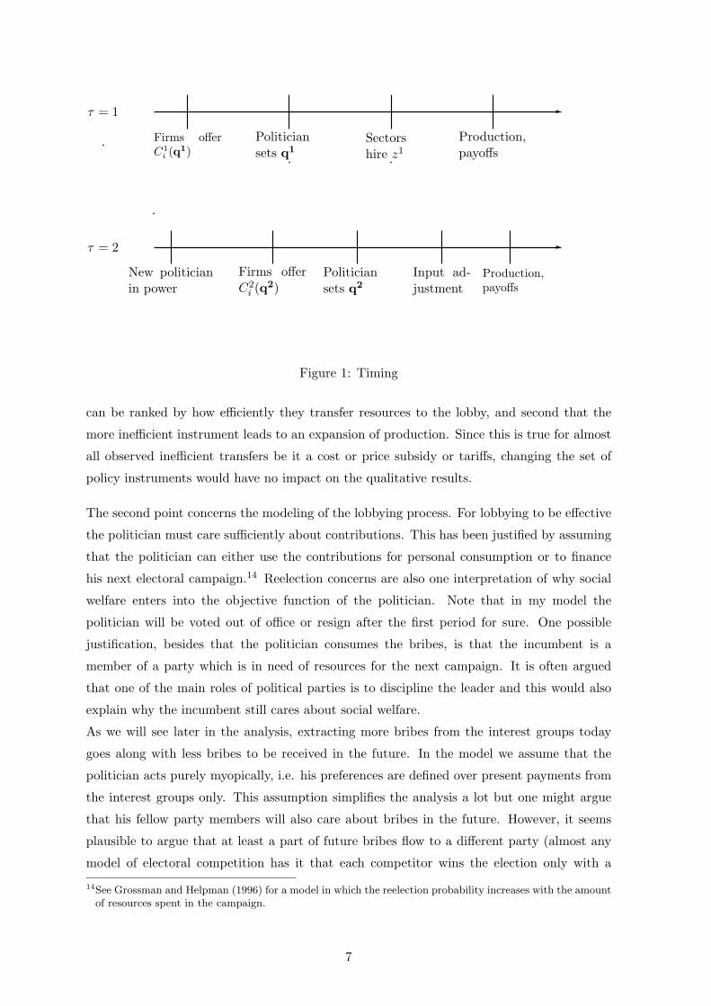
The model we consider has two periods, τ = 1, 2. In every period, each lobby first offers
a contribution schedule. After that the politician chooses a policy q1 which maximizes
his utility given the contribution schedules. Then each sector decides on its production
and therefore on the optimal amount of inputs employed. It is assumed that the industry
represented by the lobby chooses the optimal amount of inputs in every period. At the end
of the first period production takes place and payoffs are realized.
The second period is identical to the first one except that we assume that a new politician is
in power who has the same objective function as his predecessor. Again the organized sectors
lobby, followed by the implementation of the preferred policy by the politician. However if
any sector chooses to adjust its production level we assume that every worker who changes
job incurs a loss of ϑ. After this adjustment has taken place firms produce and payoffs are
realized. For simplicity we assume no discounting. The timing of the model is summarized
in figure 1.
2.2 Discussion
This subsection is devoted to the discussion of the model.
First of all we restricted the set of policy instruments available to the politician. The transfer
e can be seen as an efficient mean of redistribution while the price subsidy t leads to distortions
in the product market and is therefore less efficient. This structure is similar to Dixit,
Grossman, and Helpman (1997) where the policy instruments are also exogenously given.
What is really important in my model for the two means of redistribution is that first they
6
τ = 1 -
Politiciansets q1
Sectorshire z1
Production,payoffs
-τ = 2
New politicianin power
Firms offerC2
i (q2)Politiciansets q2
Input ad-justment
Production,payoffs
Firms offerC1
i (q1)
Figure 1: Timing
can be ranked by how efficiently they transfer resources to the lobby, and second that the
more inefficient instrument leads to an expansion of production. Since this is true for almost
all observed inefficient transfers be it a cost or price subsidy or tariffs, changing the set of
policy instruments would have no impact on the qualitative results.
The second point concerns the modeling of the lobbying process. For lobbying to be effective
the politician must care sufficiently about contributions. This has been justified by assuming
that the politician can either use the contributions for personal consumption or to finance
his next electoral campaign.14 Reelection concerns are also one interpretation of why social
welfare enters into the objective function of the politician. Note that in my model the
politician will be voted out of office or resign after the first period for sure. One possible
justification, besides that the politician consumes the bribes, is that the incumbent is a
member of a party which is in need of resources for the next campaign. It is often argued
that one of the main roles of political parties is to discipline the leader and this would also
explain why the incumbent still cares about social welfare.
As we will see later in the analysis, extracting more bribes from the interest groups today
goes along with less bribes to be received in the future. In the model we assume that the
politician acts purely myopically, i.e. his preferences are defined over present payments from
the interest groups only. This assumption simplifies the analysis a lot but one might argue
that his fellow party members will also care about bribes in the future. However, it seems
plausible to argue that at least a part of future bribes flow to a different party (almost any
model of electoral competition has it that each competitor wins the election only with a
14See Grossman and Helpman (1996) for a model in which the reelection probability increases with the amountof resources spent in the campaign.
7
certain probability). Besides, in the case where the present government is in power in the
next period for sure and has a relatively high discount factor the argument of the paper goes
through.
As mentioned above, the lobbying process itself is modeled as a menu auction. This approach
goes back to Bernheim and Whinston (1986a,b).15 The basic idea of this approach is that
lobby groups tailor their contribution to the policy which is enacted by the politician. So
implicitly it is assumed that the lobby group can commit to pay the politician according
to the contribution schedule it has offered once the policy has been implemented. Besides
this strong assumption, the menu auction approach to lobbying has the advantage that it is
tractable, as it boils down to the politician maximizing a social welfare function in which the
organized groups gain additional weight.
A further issue concerns the assumption that workers who change job in the second period
lose some amount ϑ. There are different interpretations possible. One could either assume
that there is learning on the job and so a worker who is dismissed looses some part of his
human capital. Another interpretation would be that ϑ simply measures the cost the worker
has to incur to find a new job or that the worker stays unemployed for a short period and ϑ
measures the difference between his wage and unemployment benefits.
Note that the only way to lose a job is to work in an organized sector and one might argue
that workers have to be compensated for the risk they take. This would not allow us to fix
the wage rate in the economy at one. However, as will become clear later on in the analysis,
in equilibrium it never happens that workers are fired. That is also the reason why the labor
market clearing conditions are neglected in the analysis.
I have assumed that the industry hires the efficient amount of labor in every period. This
myopic behavior neglects possible dynamic considerations. It might be optimal for the indus-
try to hire more than the efficient amount of labor in the first period to change the behavior
of the politician later on. Although this might be in the interest of the industry as a whole it
is nevertheless not optimal for a single firm belonging to the industry for standard free-riding
reasons. So implicit in this assumption is that the industry consists of many firms not able to
coordinate on some statically suboptimal capacity. This lack of coordination ability can be
justified in three ways: either a monitoring technology is missing or too costly or if contracts
on capacity can be written, by private information held by each individual firm about its
optimal capacity level. The information rents which have to be granted to all firms in this
latter case can render contractual arrangements too costly. Third it could also be the case
that capacity agreements are forbidden by the competition authorities.
15A very good overview about the theory of menu auctions and its application in the field of political economycan be found in Grossman and Helpman (2001). See also Bergemann and Valimaki (2003) for an analysisof dynamic common agency games.
8
To conclude this section I will give a short justification for the function φ(·) which measures
some social cost of transferring money to the organized groups. The first reason is purely
technical. In the absence of any redistribution costs the lobbies would extract money from the
rest of the society until the marginal utility of income of the individuals exceeds one.16 This
however makes it impossible to measure the indirect utility of the individuals in monetary
terms anymore, which in turn makes the aggregation of individual utility values and profits
accruing from the specific production factor in a social welfare function more difficult. But
there are also economic reasons to incorporate redistribution costs. Note that as the model
stands we have assumed lump sum taxation. The function φ(·) could measure the deadweight
loss accruing to society in case distorting taxes must be resorted to. Alternatively, it could
be interpreted as the administrative cost of collecting taxes and redistributing the revenue
to interest groups. One could argue that catering too much to special interests decreases the
reelection probability of the politician and therefore the value of his objective function.
3 Analysis with a Single Lobby
In this section we analyze the model in the presence of only one organized sector.17 To save
on notation we make the additional assumption that ownership is highly concentrated, so
ϕi = 0.
3.1 Preliminaries
Before we start the analysis in which one sector is organized let us take a look at the bench-
mark case in which no lobbying occurs. In this case the politician maximizes W over e and t.
Of course no transfers will be paid since by employing one of the two transfers social welfare
is reduced by the positive cost of redistribution. Formally this can be seen by looking at the
16That means that the numeraire good is no longer consumed in equilibrium.17In this section we shall drop the subscript i to indicate variables which are related to the organized group
and will simply write e, t and T (e, t) for e1, t1 and T1(e1, t1).18See the appendix for the derivation.
9
Both expressions are obviously smaller than zero if e or t are positive. The second equation
also reveals that the output subsidy is a less efficient transfer instrument compared to the
lump sum payment. When e is marginally increased by one unit the firm’s profit rises by
the same amount while increasing profits by one unit using the output subsidy costs more.
Formally, dπ(p + t) = y(p + t)dt, so the output subsidy must increase by 1/[y(p + t)] units
in order to transfer one additional unit of profit to the firm. But society bears costs of
dT = y(p+ t)dt+ ty′(p+ t)dt which, after inserting the expression for dt, yields dT = 1+ εy,t,
where εy,t > 0 is the elasticity of supply with respect to the transfer. So part of the transfer
is lost since the industry expands output. This effect is stronger the steeper the supply curve
is, i.e. the stronger supply reacts to the output subsidy.
I now turn to the case where there exists one organized group which can pay a contribution
C(q) if the politician implements a policy q. As shown by Bernheim and Whinston (1986b)
an equilibrium of the menu auction game can be characterized as follows:
Definition 3.1 {C∗(q),q∗} constitutes a Nash Equilibrium of the menu auction game if
and only if the following conditions are satisfied:
1) q∗ is feasible.
2) q∗ ∈ argmaxq aW(q) + C∗(q)
3) q∗ ∈ argmaxqW1(q) + aW(q)
4) ∃q′, q′ ∈ argmaxq aW(q) + C∗(q), such that C(q′) = 0.
The interpretation of the second condition is that the politician responds optimally to the
contribution scheme. The third condition stipulates that the optimal policy maximizes joint
welfare of the lobby group and the politician. This is not surprising as the lobby can transfer
utility to the politician without further cost. It is the last point which may be more difficult
to understand. It states that given the equilibrium contribution schedule the politician is
just indifferent between choosing the equilibrium policy q∗ and receiving C∗(q) or choosing
some other policy q′ and collecting no contributions. The meaning of this condition becomes
more apparent if we state it in the context of our model. Here q′ = 0 is the policy the
government would choose in the absence of any lobbies and hence with no contributions.
Then condition 4 says that the lobby induces the equilibrium policy q∗ at minimum cost as
the politician is just indifferent between taking the money and implementing the equilibrium
policy or neglecting the contributions of the organized group and maximizing social welfare.
In the analysis below, condition 3 will be used to determine the equilibrium policy vector
while the last condition pins down the contribution levels of the lobbies.
So far the solution to the menu auction game still seems to be complicated since one has
to maximize over a set of functions to find the lobby’s optimal strategy. Fortunately one
10
can simplify the problem considerably by focusing without loss of generality on a subset
of feasible strategies for the interest group, namely so called truthful strategies. Assuming
differentiability of the welfare and the contribution functions19 note first that the second and
third condition together imply local truthfulness in the sense that around the equilibrium
point ∇C∗(q) = ∇W1(q). Bernheim and Whinston (1986b) show that one can go even a
step further and restrict the lobby’s strategy set to globally truthful contribution schedules
without loss of generality. They show that each lobby’s best response set contains a truthful
strategy regardless of the strategies employed by other players. Furthermore, only truthful
contribution schedules are immune to pre-play communication in the presence of multiple
lobbies and are hence coalition proof. We will therefore restrict attention to these focal
strategies in the analysis to come and assume that the contribution schedule of the lobby
takes the truthful form
CT1 (q, b) = max{0,W1(q)− b1},
where b1 is some number chosen by the interest group and denotes the rent the lobby extracts
from bribing the policy maker. Note that this simplifies the problem considerably since now
one only has to solve for the optimal b1 to find the equilibrium contribution. Hence the
contribution function can be obtained by maximizing over a set of numbers and not over a
set of functions anymore.
The restriction to globally truthful contribution also makes immediately clear that the equi-
librium policy q∗ maximizes the joint welfare of the politician and the lobby. Assuming an
19Grossman and Helpman (1994) argue that differentiability of the contribution function is reasonable sincethe equilibrium does not change too much if one of the players makes small mistakes.
11
The maximization of this function yields the equilibrium policy, while the contribution func-
tion the lobby offers is obtained by employing the notion of a truthful strategy and choosing
b in a way such that the politician is exactly indifferent between a world where the interest
group is active and one where it is not. In the following proposition we summarize the result
of the static game:
Proposition 3.1 The equilibrium policy of the static game is given by t∗ = 0 and e∗ im-
plicitly defined by 1 = aφ′(e∗).
The lobby offers the following contribution schedule: CT ∗ = e− e∗ + aφ(e∗).
Proof: See the appendix.
This result is reminiscent of Dixit, Grossman, and Helpman (1997) as the (more) inefficient
transfer instrument is not used in equilibrium. To understand this result remember that
the lobby and the politician maximize their joint welfare in equilibrium. Hence, the output
subsidy is not used as it leads to a loss of resources. Turning to the contribution function,
note that the lobby reimburses the politician exactly for the loss in social welfare it induces
by influencing the policy choice. Evaluating CT ∗ at the point e∗ immediately reveals that the
policy maker gets exactly aφ(e∗) as a contribution and so is exactly indifferent between setting
e = 0 (which is his default policy choice in the absence of a lobby group) and implementing e∗.
Note therefore that the politician gains nothing if only one interest group is active, since he
is precisely held down to his reservation utility and the lobby captures all the surplus which
is generated by the lobbying process. This is a very important property of menu auctions,
as we will see again later in the analysis. Each lobby’s rent is determined by the amount the
interest group adds to the joint surplus of the politician and the lobby by becoming active
and bribing the policy maker. That e∗ − aφ(e∗) corresponds to the added joint surplus can
easily be seen. Without the lobby, the politician sets q = 0 and the joint surplus is given
by aW(e = 0, t = 0). With an active lobby the optimal policy increases joint welfare by e∗
as the lobby gets an additional weight of 1, but welfare is reduced by the redistribution cost
aφ(e∗). The added joint surplus is of course larger if the politician cares less about society’s
well-being as measured by a decrease in the parameter a.
3.3 The Two Period Model
3.3.1 The Final Period
As shown by Bergemann and Valimaki (2003), the same techniques as developed by Bernheim
and Whinston (1986a,b) can be applied to solve dynamic menu auction games. The aim of
this section is to show how the second period output subsidy t2 depends on first period policy,
12
especially on the subsidy t1 granted in τ = 1.
We proceed by backward induction and begin our analysis in the second period. Assume that
the politician in period 1 has implemented a policy q1 = (t1, e1) which leads the organized
industry to employ an amount z1(p + t1) of labor.20 When the second period politician has
to decide about the policy q2, he now also takes into account that a price subsidy in period
2 which is different from t1 leads to a welfare loss. This is due to the fact that the firm
responds optimally to equilibrium prices and adjusts the amount of labor employed. Since
all workers who have to change their job lose an amount ϑ of income, welfare in the second
period is given by
W = W0 +W1
= m + S[p]− T(e2, t2
)− δϑ
[z1(p + t1)− z2(p + t2)
]− φ
[T (e2, t2)
]+ π
[p(t2) + t2
]+ e2.
δ is a dummy variable taking the value 1 if t1 ≥ t2 and −1 otherwise. It is obvious that the
second period politician will never choose a policy which implements a higher price subsidy
than the one already in place. In the following analysis we will assume that t1 is large enough,
postponing the exact characterization of t1 until the period 1 lobbying game is examined.
Hence, all values derived in this section are properly interpreted as maximum values given
that the output subsidy in the first period was at least as large. Since the maximization
problem is the same as in the static case, the policy maker will not use the efficient transfer
e2 in the absence of an organized lobby group. However, given that a positive price subsidy
has been implemented in the first period, the politician has an incentive to at least partially
sustain the policy. This can be seen by examining the first order condition of W with respect
to t2:
∂W∂t2
= a[−ty′(p + t2)− φ′[T (e, t)]
[y(p + t2) + ty′(p + t2)
]+ ϑz′2(p + t2)
]= 0.
Under the assumption thatW is a concave function, the equation above has a unique solution
t−1 > 0. It is important to note that this solution depends on the price subsidy in period one
t1 only insofar as t−1 must be smaller than t1. If this were not the case, the policy maker
would create reallocation of workers instead of avoiding it. Formally, δ would turn negative
and one would have to subtract ϑz′2(t2)[p + t2] in the first order condition above and the
whole expression would be negative except at t−1 = 0. So t−1 denotes the maximal value of
the output subsidy in the second period under the assumption that the subsidy in the first
period was at least as large.
The solution t−1 will obviously be larger the smaller φ′(·) and y′(p + t) are, i.e. the smaller
the cost of transferring money to the lobby via the output subsidy.
20Remember that throughout the analysis, subscripts denote the lobby group while superscripts stand for thetime period.
13
As in the static case, when deciding over the policy the politician maximizes the following
expression:
G2 = aW +W1
= a[m + S[p(t2)]− T (e2, t2)− ϑ
[z1[p + t1]− z2[p + t2]
]− φ[T (e2, t2)]
]+(1 + a)
[π[p + t2] + e2
]Assumption 3.1 G2 is quasiconcave in t2 and exhibits an interior maximum with respect to
e2.
This assumption is necessary since G2 depends on t2 in two ways: first, increasing t2 leads
to a welfare loss lowering G2 and this loss is the larger the larger t2. On the positive side is
that increasing t2 saves reallocation costs. This positive effect depends on the labor demand
function which normally is convex. Hence we subtract a convex function from a convex
function and the assumption makes sure that the welfare loss dominates, leading to a well-
behaved objective function. The interior solution with respect to e2 is guaranteed if the
redistribution cost function φ(·) is not too convex and simplifies the analysis considerably.
We will now provide the solution to the lobbying game in the second period.
Lemma 3.1 Let t2 be the solution to the following equation:
−(1 + a)(t2y′[p + t2]
)+ aϑz′(t2) = 0.
In the second period the politician will implement q2∗ = (e2∗, t2∗), where t2
∗ = min{t1, t2}and e2∗ solves aφ′[T (e2∗, t2
∗)] = 1.
Proof: See the appendix.
The interpretation of this lemma is as follows. First, given that e2 > 0 in equilibrium, the
lobby will extract resources from the policy maker until its marginal benefit equals marginal
redistribution cost. t2 is characterized by a joint optimality condition of the politician and the
interest group. Note that t2 is the maximal sustainable output subsidy in the second period.
The equilibrium transfer will be smaller than t2 whenever the subsidy implemented in the
first period is smaller. This is an important property of the model. When the lobby tries to
increase the output subsidy in the first period it automatically increases the second period
subsidy by the same amount (so t2 as a function of t1 is the identity function). From this
reasoning, one can immediately deduce why no worker reallocation takes place in equilibrium.
14
3.3.2 The First Period
The above analysis was carried out under the assumption that the price subsidy implemented
in the first period is positive. This must be the case in order for the equilibrium policy in
the second period to entail a positive subsidy. We will now show that in the first period the
interest group can decide between two options. First, by trying to receive the subsidy, which
comes at a cost in the current period, since part of the transfer which must be paid is lost
but increases the rent which can be captured in the second period. Or secondly, by lobbying
solely for the efficient transfer, which has no effect on the future.
In order to determine the equilibrium policy of the game we therefore have to investigate first
how the rent in the second period varies dependent on the price subsidy in the first period.
We start with an important lemma.
Lemma 3.2 The optimal price subsidy in the first period t1∗ is equal to t2
∗.
The proof is obvious and therefore we will only give the intuition for the result. We have
already established in the last section that the politician in the second period will never
increase the level of the price subsidy, hence t2∗ ≤ t1
∗. Now assume that the price subsidy
in the first period strictly exceeds the one in the second, i.e. t1∗
> t2. Then the interest
group and the politician can improve on their joint welfare by reducing the price subsidy in
the first period and using the efficient transfer instead. By doing this the rent of the lobby
in the second period remains unchanged (since t2∗ does not change) but the joint welfare in
the first period increases as distortions on the product market are avoided.
We are now in the position to examine the rent the lobby receives in the second period
depending on the subsidy in the first one. Again, the politician is exactly indifferent be-
tween receiving payments from the interest group and implementing his preferred policy and
neglecting contributions altogether. Note that the default policy the politician chooses in
absence of the lobby is given by e2 = 0 and t−1. Since it is a priori not clear whether t−1 is
smaller or larger than t2∗ one has to distinguish between two cases.
First consider the case where t−1 > t2∗. Since t2
∗ and e2∗ are implemented in equilibrium
the rent b2 for the lobby is given by the following condition.21
aW(t2∗) = aW(t2∗, e2∗) + C2(e2∗, t2∗)
⇐⇒
aW(t2∗) = aW(t2∗, e2∗) + π(p + t2∗) + e2∗ − b2
21Remember that given t2∗
it is optimal to have t1∗
= t2∗. But that means that the politicians default policy
is also t1∗
and not t−1 anymore!
15
Beside the redistribution cost, the welfare of the society is the same. Defining T as the
equilibrium amount of transfers society has to pay with aφ′(T ) = 1, we can write b2 as
follows:
b2 = a[φ(t2∗y(p + t2
∗))− φ(T )]
+ π(p + t2∗) + e2∗ (5)
Now it is important to remember that t2 and t1 vary exactly together in equilibrium as long
as t1 is smaller than t2, the maximum output subsidy in the second period. Therefore, one
could write b2 as a function of t1 as well by replacing t2∗ with t1. In what follows it will be
convenient to think of b2 as directly controlled by the choice of the subsidy in the first period.
One can immediately see that inducing a positive subsidy in the first period might be bene-
ficial for the lobby since it does not have to compensate the policy maker for the full amount
of redistribution costs anymore. However, note also that implementing the price subsidy
causes a subtle cost for the lobby. Since the sum of transfers to the lobby is bounded by the
redistribution cost function at T , the amount of the lump sum transfer in period 1 shrinks
whenever the output subsidy is positive, i.e. e2∗ = T − t2∗y(p + t2
∗). In the following lemma
we will show that this latter effect dominates whenever t−1 > t2∗.
Lemma 3.3 If t−1 > t2∗ the interest group will only lobby for the efficient transfer e.
Proof: See the appendix.
The intuition behind this result is that for t−1 > t2∗ it is necessary that the cost of redistribu-
tion is very low. Hence the cost saving in the second period from inducing the output subsidy
in the first period is rather low and the interest group prefers the efficient transfer.22 Thus,
the result makes clear that a politician who puts only little weight on welfare and caters a
lot to interest groups (i.e. a politician with a small value of a) has an ambiguous effect on
welfare: on the one hand total transfers increase but on the other hand, the more efficient
transfer instrument is used.
Let us now turn to the second case where t−1 < t2∗. Here, the contributions of the interest
group make it optimal for the politician to increase the subsidy beyond his default policy.
To examine the incentives of the lobby to receive such a transfer scheme, we again have to
investigate how the rent in the second period depends on the subsidy in the first one. The
rent of the lobby is calculated in the usual manner by compensating the politician exactly
for the change in welfare induced by the lobbying process. Specifically, the rent b2 can be
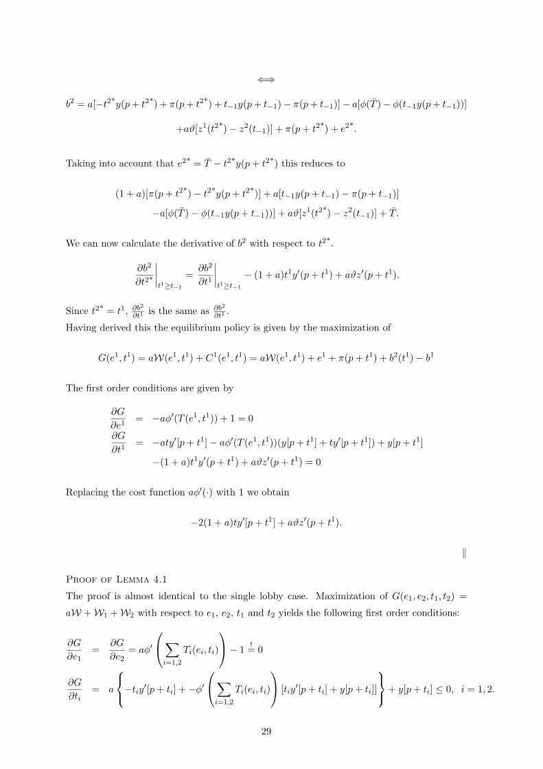
22This point can most easily be seen by looking at the extreme case where total transfers are bounded by Tbut no further redistribution costs accrue. In this case b2 = π(p+ t2
∗)+ e2∗ = T − t2
∗y(p+ t2
∗)+π(p+ t2
∗)
and one can immediately see that setting t2∗
equal to zero is optimal. The reason is that the lobby does nothave to compensate the politician for any redistribution costs and therefore gets transfers for free.
As the labor demand function z(p + t) is strictly increasing whenever y′(·) 6= 0, the output
subsidy will be positive in equilibrium. Therefore, we have established that the inefficient
transfer is used despite the fact that an efficient redistribution device is available. The
intuition for this result can be derived from our discussion of the rent b2. It is shown in
the appendix that if the interest group expands the output subsidy beyond t−1 the marginal
change in the rent is given by
∂b2
∂t1
∣∣∣∣t1≥t−1
= −(1 + a)t1y′(p + t1) + aϑz′(p + t1).
The interest group thus faces two effects. The first effect is negative and measures the loss
of resources the output subsidy entails. This loss accrues both to society (and is therefore
weighted with a) and to the lobby which forgoes some amount of the transfer.23
But as mentioned above, a positive subsidy in the first period leads to overcapacities in the
23Remember that the total sum of transfers society has to pay for is fixed at T . If the politician wantsto transfer some fixed amount of money to the interest group by using the subsidy the deadweight lossassociated with this transfer results in a higher payment for the society. That means that the interest groupcan extract only a smaller amount of the lump sum transfer. It is for this reason that the loss of resourcesis additionally weighted with 1.
18
industry and makes the politician reluctant to cut back the transfer in the second period.
In the case we consider where t−1 < t2∗, the parameters are such that the policy maker is
nevertheless willing to tolerate some amount of worker reallocation in the absence of a lobby.
However, this decreases his reservation utility and for this reason the interest group has to
pay less compensation. Thus, as t1 is increased beyond t−1, the interest group gains exactly
the additional welfare loss which would be inflicted on society if the lobby was absent in the
second period.
The comparative statics of the equilibrium output subsidy are straightforwardly calculated.
As one would expect, the subsidy is increasing in ϑ, the welfare cost of worker reallocation.
A more surprising effect is obtained when considering the parameter a. As the sign of ∂t1∗
∂a is
the same as the derivative of the equilibrium condition for t1∗ stated in the proposition, we
have
sign[∂t1
∗
∂a
]= sign
[−2t1
∗y′(p + t1
∗) + ϑz′(p + t1∗)]
> 0.
The last expression is positive at the equilibrium value since the first (negative) term is
weighted less while the second positive term is weighted more compared to the equilibrium
condition. Thus ceteris paribus politicians who care more about social welfare will implement
a higher output subsidy. The explanation for this phenomenon is simple: a higher value of
a means that the politician cares more about society’s wellbeing relative to interest group
profit. Hence, the policy maker is more willing to avoid reallocation cost and to tolerate
less industry profits. We subsume the comparative statics of the single lobby model in the
following corollary:
corollary 3.1 The implemented level of the price subsidy is increasing in reallocation cost
ϑ and the politician’s concern for social welfare a.
To understand the condition for the equilibrium value of the subsidy, note that the interest
group’s willingness to pay24 for it consists of two parts: the profit generated by it and the
future rent which can be obtained. Hence, when the lobby decides whether to pay for the
output subsidy, it takes into account the loss of resources entailed in the first period (which
is again given by (1 + a)t1y′(p + t1)). Adding up the first period loss and the change in the
second period’s rent yields the condition stated in the proposition.
Given the optimal value of the subsidy, the lump sum transfer e1 is expanded until the
marginal profit to the firm equals marginal redistribution cost. Once the equilibrium policy is
fixed, the contribution schedule can easily be obtained by employing the notion of truthfulness
and pushing the politician down to his reservation utility.
24Remember that we are still considering an equilibrium in truthful strategies so the contribution scheduleoffered just reflects willingness to pay.
19
In summary, we have established that in a dynamic setting strategic considerations might
lead interest groups to lobby for an inefficient transfer. The key in the model is that the
preferences of succeeding politicians can be altered through an output subsidy. Specifically,
compensation for the second period’s policy maker can be lowered as sustaining the output
subsidy avoids social costs through worker dismissal.
4 Multiple Lobbies
One cumbersome property of the menu auction approach to lobbying is the fact that with
two or more lobbies competition between organized groups gets extremely fierce. If one
considers a model with inefficient transfer instruments only, the result that the benefits from
lobbying activity go down is still intuitive. However if one allows for the availability of an
efficient transfer the rents lobbies can appropriate are immediately driven down to zero. To
see the point first note that in static settings only the most efficient redistribution device
is employed. Since the politician must still get his reservation utility each interest group
must design its contribution schedule in such a way that the policy maker is just indifferent
between catering to this interest group or disregarding it altogether. Put differently each
interest group must compensate the politician exactly for the joint welfare change of society
and all other lobby groups induced by the policy change. So if only the efficient redistribution
device is used, how does the utility of the politician change upon a new interest group entering
the political arena? Since the well-being of the society as a whole is not affected by lump sum
redistribution and the politician does not care which lobby gets the money, the utility of the
politician is unaffected by the entry of a new lobby. That means that the policy maker does
not lose anything if he disregards one lobby and caters instead to the other one(s), resulting
in a very strong bargaining position. Hence the competition between interest groups is of a
Bertrand type. By raising its contribution (i.e. lowering the rent) marginally over its rival
each lobby can appropriate all the funds which are available. Consequently interest groups
will raise their bids until their rent is zero.
This result raises two concerns: first only efficient redistribution takes place in equilibrium,
which can hardly be reconciled with reality. Second, each interest group has nothing to
gain from the lobbying process and would be as well off by unilaterally withdrawing its
contributions. It is important to note that this prisoners dilemma type of situation does not
occur if only inefficient transfer instruments are available. As inefficient redistribution causes
welfare costs for which the politician must be compensated, each lobby is less aggressive
leading to positive equilibrium rents. To save the plausibility of this type of model the extant
literature resorted to the following argument:25 since lobbies fare so poorly in equilibrium
25See Dixit, Grossman, and Helpman (1997).
20
they will ex-ante agree on a constitution specifying that interest group are allowed to lobby
only for inefficient transfers. Since it is unclear whether such a contract is enforceable before
a court the argument relies at least partially on a repeated game setting in the background.
This being said, it seems to be worthwhile to investigate whether competition between lobbies
has the same detrimental effect on interest group payoffs in our model.
Throughout we will stick to the same assumptions as in the monopolistic lobby case, except
that we now allow for a second organized sector.26 We will also assume that both industries
are completely symmetric and are characterized by the same production technology.
4.1 The Static Game
To illustrate the arguments outlined above we will start with the static case. The subscripts
1 and 2 denote the two lobbies.
In the presence of two lobbies which submit truthful contribution schedules the equilibrium
policy is determined by the maximization of the following function:
G(e1, e2, t1, t2) = aW +W1 +W2. (8)
As in the setting with only one lobby only the efficient transfer will be used.
Proposition 4.1 In equilibrium t∗1 = t∗2 = 0. The efficient transfers e∗1 and e∗2 are set such
that aφ′(e∗1 + e∗2) = 1.
Proof: See the appendix.
First note that the total amount of resources redistributed does not change compared to
the single lobby case. Since the cost of redistribution depends on the sum of transfers the
marginal payment to compensate the politician for the last unit of redistribution still equals
marginal benefit of the lobby and is therefore equal to one. The second property of the
equilibrium worth emphasizing is that although the total sum of transfers is fixed at T it is
not clear how T is distributed among the groups. This indeterminacy is due to the fact that
the policy maker is indifferent about the exact allocation of resources as long as only lump
sum payments are used. This leads us directly to the investigation of the equilibrium rents
b∗i , i = 1, 2.
As outlined before given b∗j the rent bi is determined such that the policy maker is indifferent
between disregarding lobby i’s contribution and just dealing with lobby j, j 6= i, and taking
26Since two lobbies are sufficient to drive rents down to zero in the extant literature this assumption seemsobvious. An extension to more than two lobbies has no impact on our core results (see section 4.2).
21
both contributions into account and changing equilibrium policy accordingly. First of all we
need to determine which policy would have been chosen in the absence of one lobby. Since
only two industries are organized we can resort to the results of the previous section. Clearly,
each lobby would get an amount of T of the efficient transfer. We denote the transfer to
lobby j in the absence of lobby i with ej . Formally the contribution schedule C1(e1, b∗1) of
lobby 1 must satisfy the following requirement:
aW(e2) + C2(e2, b∗2) = aW(e∗1, e
∗2) + C2(e∗2, b
∗2) + C1(e∗1, b
∗1).
The left hand side is the payoff of the politician with just lobby 2 active while at the right
hand side both lobbies are active. Note first that the welfare of the society as a whole remains
unchanged since the sum of transfers is not altered. Moreover as e2 = T and e∗2 = T − e∗1 we
can rewrite the above condition employing truthful strategies:
T − b∗2 = T − e∗1 − b∗2 + e∗1 − b∗1 ⇒ b∗1 = 0.
The problem for lobby 2 is exactly the same so we can conclude that both interest groups
derive no benefit from the lobbying process. Thus the static model replicates well known
results from the extant literature. Both lobbies bid for transfers which are available in fixed
total sum so competition drives their payoffs down to zero.
4.2 Analysis of the Dynamic Game
Again we proceed by backward induction and first analyze the second period. Total welfare
in the society is given by an expression analogous to the monopolistic case:
W = W0(e21, e
22, t
21, t
22) +W1(e2
1, e22, t
21, t
22) +W2(e2
1, e22, t
21, t
22) =
m+S[p]−∑i=1,2
Ti(e2i , t
2i )−
∑i=1,2
δiϑ[z1i (p+t1i )−z2
i (p+t2i )]−φ
∑i=1,2
Ti(e2i , t
2i )
+∑i=1,2
{πi[p(t2i )+t2i ]+e2i }.
δi is an indicator variable which takes on the value 1 if t1i > t2i (resulting in a compression
of the amount of labor hired in industry i) and the value −1 otherwise. Some results of the
single lobby case naturally carry over to the competitive case. Obviously the politician has no
incentive to increase the output subsidy beyond the level stipulated in the first period. Second
for the same reasons as in the monopolistic lobby case there will be no worker reallocation
in equilibrium or, put differently, the subsidy implemented in the first period will not exceed
the one in the second period.
As in the single lobby case we first investigate the maximal sustainable output subsidy in the
22
second period, neglecting the equilibrium level until we analyze the first period of the game.
For this we maximize the objective function of the politician
G2(e21, e
22, t
21, t
22) = aW(e2
1, e22, t
21, t
22) +W1(e2
1, e22, t
21, t
22) +W2(e2
1, e22, t
21, t
22)
we respect to the policy instruments. The following lemma comprises the results.
Lemma 4.1 Let ti be defined by
−(1 + a)tiy′(p + ti) + aϑz′i(ti) = 0, i = 1, 2.
Second period equilibrium policy is given by q2∗ = (t2i∗, e2
i∗)i=1,2 with t2i
∗ = min{ti, t1i } where
t1i denotes the output subsidy for industry i implemented in the first period.
The equilibrium lump sum transfers are determined by aφ′(∑
i=1,2 Ti(t2i∗, e2
i∗))
= 1.
Proof: See the appendix.
The result is striking if one compares the condition for the maximal sustainable output
subsidy with the single lobby case. The expressions are equal, meaning that the presence of an
additional lobby does not alter the set of possible output subsidies which can be implemented
by the interest groups. Again, once the level of output subsidies is fixed the amount of the
efficient transfer to each lobby is obtained by equalizing marginal benefit with marginal
redistribution cost.
However for the determination of the policy vector actually chosen by the politician one
again has to look at the incentives to introduce the inefficient transfer in the first place.
As we know already from the analysis of the single lobby case the crucial factor is how the
second period equilibrium rent changes with t1i , the output subsidy implemented in the first
period. To obtain this rent we first have to derive the default policy which is implemented
in the absence of a lobby.27 Of course if an interest group is not active it will not receive the
efficient transfer. The level of the output subsidy instead is determined by the derivative of
G−1 = aW +W2 with respect to t21. It can be shown (see the appendix) that
∂G−1
∂t21= −(1 + a)t21y
′1(p + t21)− y1(p + t21) + aϑz′1(t
21).
It is important to note that the maximizer of this derivative t−1 ≥ 0 is always smaller
compared to the monopolistic setting. Again we have to distinguish between two different
cases as in the single lobby case. If t−1 > t11∗ there is no incentive for the interest group to
obtain the output subsidy. In what follows we focus exclusively on the more interesting case
27The following analysis is conducted for lobby 1, the problem for lobby 2 is exactly the same.
23
where t−1 < t11∗.
Knowing the default policy of the politician it is by now straightforward albeit somewhat
tedious to calculate the equilibrium rent of lobby 1.
Lemma 4.2 The equilibrium rent of lobby 1 in the second period b21∗ is given by
b21∗ = (1+a)
[π(p + t21
∗)− t21∗y(p + t21
∗)]+a[t−1y(p+t−1)−π(p+t−1)]+aϑ
[z1(t21
∗)− z2(t−1)].
Proof: See the appendix.
The first term measures the welfare loss associated with an output subsidy of t21∗ which
is weighted with 1 + a, the weight attached to industry profits by the politician. This is
intuitive as the use of the output subsidy reduces the amount of additional profits which can
be shifted to the lobby. Both other terms are positive and well known from the discussion of
the equilibrium rent in the monopolistic lobby case. The first one displays how much of the
output subsidy and thus loss of resources the politician would have been willing to tolerate
in the absence of the interest group. The second one indicates the cost of worker reallocation
society would have to bear if group one was not active.
It might be surprising that this expression is very similar to the monopolistic case. Comparing
the formula above with equation (6) the first thing to note is that in the competitive case the
interest group does not have to compensate the politician for any redistribution cost. This
makes sense since in the monopolistic case the lobby had to reimburse the policy maker for
the additional redistribution cost caused by active lobbying. Here however, if lobby 1 is not
active all resources available for redistribution will flow to lobby 2 resulting in social cost of
aφ(T ) anyway. Besides this the expressions for second period rents are identical but note
that t−1 is smaller in the competitive case.
For the determination of equilibrium policy however the crucial factor is how b21∗ behaves as
t11 and therefore t21∗ changes. Assuming that t−1 < t21
∗ the derivative of b21∗ with respect to
t11 is given by
∂b21∗
∂t11= −(1 + a)t11y
′1(p + t11) + aϑz′1(t
11). (9)
Note that this expression is exactly identical to the monopolistic case. We are now able to
pin down the equilibrium policy vector.
Proposition 4.2 The equilibrium output subsidies t1i∗, i = 1, 2 are implicitly defined by
−2(1 + a)t1i∗y′i(p + t1i
∗) + aϑz′i(p + t1i∗) = 0.
The equilibrium lump sum transfers e1i∗, i = 1, 2 are given by aφ′
(∑i=1,2 Ti(e1
i∗, t1i
∗))
= 1.
24
Proof: See the appendix.
Hence competition between lobbies only affects the amount of the efficient transfer the interest
groups can appropriate. The level of the output subsidy does not change. The intuition for
this result is as follows. In the competitive case lobby 1 competes for transfers against lobby 2.
But in the monopolistic case the interest group also takes into account that if it increases the
output subsidy marginally, the amount of the efficient transfer it can appropriate goes down.
One can therefore say that the lobby competes against itself. Furthermore equilibrium policy
is characterized by a joint optimality condition and for the politician it makes no difference
which lobby suffers from a reduction in available transfers. Hence the willingness to pay for
the subsidy on the interest group’s side and the willingness to give on the politician’s side
remain unchanged.
Since the equilibrium condition does not change compared to the monopolistic case the same
interpretation and the same comparative statics apply. A more interesting point concerns
the comparison of social welfare. First of all remember that in the monopolistic case a
necessary condition for a positive output subsidy was that the second period policy maker
was sufficiently reluctant to transfer resources inefficiently. We stipulated that if the costs
of redistribution are too low it is optimal for the interest group to lobby for the efficient
transfer only. Intuitively, as the lobby gets any transfer almost costlessly it does not pay
to waste resources in the first period to influence the preferences for redistribution of the
succeeding politician. This scenario happens in the competitive case only with a smaller
probability. Here the presence of another lobby makes it more costly to obtain transfers
since interest groups compete against each other. Hence more organized industries make
the political equilibrium more inefficient since political insulation of policies becomes more
attractive.
A second effect going in the same direction does not concern the probability that the output
subsidy is used but the total amount of inefficient redistribution. Since equilibrium subsidies
are the same for each lobby independently of the degree of competition, total waste in the
economy increases as the number of organized industries goes up. It is also straightforward
to see that if the number of active lobbies grows sufficiently large, all resources available for
redistribution will be exhausted by subsidy payments. Hence if a society exhibits a growing
number of organized special interests, lump sum transfers will no longer be observed in
equilibrium.
We can therefore state that more competition among lobbies leads to a more and more
inefficient political equilibrium.
25
5 Conclusion
The paper has developed a dynamic theory of inefficient redistribution to interest groups.
It did so by considering a two period game where in each period interest groups have the
possibility to bribe the politician in exchange for a favorable policy. As a main point we
have shown that inefficient transfers can occur in equilibrium and that competition between
interest groups is not effective in eliminating them but even makes things worse. The paper
therefore contributes to our understanding of the lobbying process.
However we have treated some aspects of the game as a black box. First we have an incom-
plete understanding of which industries manage to get organized and how possible incentive
problems within an interest group are overcome. Second politicians are hardly unitary actors
but are members of organizations which constrain their behavior. To our knowledge a more
explicit modeling of parties has not been embedded into the lobbying literature so far.28 A
model of the inner workings of parties would also help us to give a more solid microfoundation
for the objective function generally assumed in the lobbying literature. For this point see
also the discussion in the second section of this paper. Finally instead of assuming that both
social welfare and received bribes increase the reelection probability one should incorporate
the voting behavior explicitly into the model. Coate (2004a,b) goes along these lines and finds
interesting results. More campaign spending does not automatically lead to better reelection
prospects as voters anticipate that generous support of the campaign by interest groups must
be paid back later in form of favorable policies. It is hence questionable whether more funds
translate into higher reelection probabilities.
All of these topics seem to be worth future investigation.
28The role of political parties in general is only poorly understood so far. See Caillaud and Tirole (1999),Caillaud and Tirole (2002) and Levy (2004) for first steps in that direction.