Political machinery: did robots swing the 2016 USpresidential election?∗

Carl Benedikt Frey,† Thor Berger,‡ and Chinchih Chen§

March 14, 2018

Abstract

Technological progress has created prosperity for mankind at large, yet it has always

created winners and losers in the labour market. During the days of the British Industrial

Revolution a sizeable share of the workforce was left worse off by almost any measure

as it lost its jobs to technology. The result was a series of riots against machines. In

similar fashion, robots have recently reduced employment and wages in US labour mar-

kets. Building on the intuition that voters who have lost out to technology are more

likely to opt for radical political change, we examine if robots shaped the outcome of the

2016 US presidential election. Pitching technology against a host of alternative explana-

tions, including offshoring and trade exposure, we document that the support for Donald

Trump was significantly higher in local labour markets more exposed to the adoption of

robots. A counterfactual analysis based on our estimates shows that Michigan, Pennsyl-

vania, and Wisconsin would have swung in favour of Hillary Clinton if the exposure to

robots had not increased in the immediate years leading up to the election, leaving the

Democrats with a majority in the Electoral College.

JEL: J23, J24, J31, N60, O14Keywords: automation, industrial revolution, labour markets, technological change,political economy

∗We are grateful for helpful comments and suggestions from the editor, Abigail Adams, an anonymousreferee, and participants at the Oxford Review of Economic Policy seminar, as well as to Robert Allen for kindlysharing data. Chen and Frey gratefully acknowledge funding from Citi. Any remaining errors are our own.

†Oxford Martin School, University of Oxford, e-mail: carl.frey@oxfordmartin.ox.ac.uk‡Oxford Martin School, University of Oxford, and Department of Economic History, School of Economics

and Management, Lund University, e-mail: thor.berger@ekh.lu.se§Oxford Martin School, University of Oxford, e-mail: chinchih.chen@oxfordmartin.ox.ac.uk

1

1 Introduction

Was the outcome of the 2016 US presidential election shaped by workers losing out to au-tomation? According to a recent poll of unemployed Americans who were able to work,more than a third identified automation as a prime reason for their misfortunes (Hamel et al.,2014). Moreover, a staggering 72 per cent of surveyed Americans fear a future in whichcomputers and robots can do more human jobs, while 85 per cent favour policies to restrictthe use of machines to hazardous jobs (Pew Research Center, 2017). Even though the causesof the populist backlash in America and Europe are far from conclusive, parallels have beendrawn with the machinery riots of the British Industrial Revolution, when ‘Luddites’ smashedpower looms in fear of losing their jobs. A post-election article in The Wall Street Journal

featuring the headline ‘Trump’s focus on jobs, globalization and immigration tapped anxietyabout technological change’ speaks to the frequent belief that automation was a real cause ofvoter concern. Despite such beliefs, empirical efforts to examine the extent to which automa-tion shaped the outcome of the US presidential election have remained scant. What is clear isthat the vote for Donald Trump was a vote against the status quo: according to the exit polls,82 per cent of voters believed that the Republican candidate would perform best in bringingabout change, while the corresponding figure for Hillary Clinton was a meagre 14 per cent.

This paper examines the link between workers exposure to automation and voting patternsin the 2016 US presidential election through the lens of economic history. Our analysis buildson two sets of observations. First, technological change in the short to medium term is rarelya Pareto improvement: as automation has made inroads into a wider set of industries andoccupations, it has left a sizeable fraction of the workforce worse off. In particular, the sharpreduction in middle-income jobs in the US economy cannot be explained without referenceto the disappearance of ‘routine jobs’—i.e. occupations mainly consisting of tasks followingwell-defined procedures that can easily be automated (Autor et al., 2003; Acemoglu andAutor, 2011). As traditional middle-income jobs have dried up, many workers have shiftedinto low-income service occupations (Autor and Dorn, 2013), while others have dropped outof the workforce altogether (Cortes et al., 2016a). According to Eberstadt’s (2016) timelybook, Men Without Work, 24 per cent of prime-aged men in the US will be out of work by2050 at current trend. A prime explanation is the robot revolution, which has contributedto both joblessness and wage reductions, especially among American men (Acemoglu andRestrepo, 2017).

Second, the economics of automation cannot be separated from its politics. For ordinaryworkers, their skills constitute their capital; it is from their human capital that they derivetheir subsistence. Because automation is accompanied by creative destruction in employ-ment, which often comes with social costs—including vanishing incomes, forced migration,skill obsolescence, and episodes of unemployment—it threatens not only the incomes of in-

2

24

68

1012

Cha

nge

in R

epub

lican

two−

part

y vo

te s

hare

2016

(T

rum

p) v

s. 2

012

(Rom

ney)

0 1 2 3 4Changes in the exposure to robots

Notes: This figure presents a non-parametric illustration of the county-level relationship between percentagepoint differences in the Republican two-party vote share between the 2016 and 2012 elections based on datareported in Dave Leip’s Atlas of US Presidential Elections and changes in the exposure to robots between theimmediate years prior to each election based on data from the International Federation of Robotics and theAmerican Community Survey respectively, which we describe in more detail in the main text. To constructthe figure, we sorted all observations into 30 equal-sized bins and plotted the mean change in the Republicantwo-party vote share versus the exposure to robots within each bin, while the line corresponds to a fitted OLSregression based on the underlying (ungrouped) data.

Figure 1: Exposure to robots and the vote for Trump

cumbent producers but also the power of incumbent political leaders (Acemoglu and Robin-son, 2013). The reason is simple: if workers who have lost out to automation do not acceptlabour market outcomes, they will resist the force of technology through non-market mecha-nisms, such as political activism (Mokyr, 1990, 1998; Mokyr et al., 2015). The British Indus-trial Revolution provides a case in point. The downfall of the domestic system—which wasgradually displaced by the mechanized factory—inflicted substantial social costs on workers,leading them to rage against the machines that pioneers of industry marvelled about. The1779 riots in Lancashire and the Luddite risings of 1811–13, are only two of many attemptsto bring the spread of machines to halt (Mantoux, 2013). Although the Industrial Revolutionbegan with the arrival of the factory, it ended not just with the construction of the railroads butalso with the publication of the Communist Manifesto. While the accelerating pace of tech-nological progress paved the way to modernity, it also bred many political revolutionariesalong the way.

Against this background, we examine whether the increased adoption of robots causedAmerican voters to opt for radical political change. A recent study by Acemoglu and Re-strepo (2017) documents that the diffusion of robots across US labour markets has causedemployment and wage reductions in particular among workers in blue-collar jobs without

3

a college degree. Notably, these are precisely the voter groups that shifted in favour of theRepublican party in the 2016 election: Trump won the group of non-college educated whites,for example, by a wider margin than any candidate going back to 1980. Building on theseobservations, we explore if robots shaped the outcome of the 2016 US presidential election.

Figure 1 presents a non-parametric illustration of our key finding, documenting the pos-itive relationship between differences in the Republican two-party vote share between the2016 and 2012 elections and changes in the exposure to automation across electoral districts.We show that this relationship remains similar also when controlling for a range of other base-line demographic and economic factors, specialization in manufacturing, and differences inthe share of employment that falls in occupations and industries that are more exposed tooffshoring, routinization, and trade. The observed relationship also remains when we factorout state-level shifts in voting patterns and exploit differences in exposure across electoraldistricts located within the same state. To account for the potential endogeneity of robot ex-posure, we also present additional instrumental variable (IV) estimates that exploit historicaldifferences in industrial specialization across local labour markets and the adoption of robotsin countries other than the US to show that this relationship is presumably causal. As a finalempirical exercise, we perform a series of back-of-the-envelope calculations to examine howthe outcome of the 2016 election would have changed under different counterfactual levels ofrobot adoption. All else equal, these exercises suggest that in a scenario where the exposureto robots had not increased in the immediate years leading up to the election, the ElectoralCollege would have been won by the Democratic candidate. Although these findings natu-rally should be interpreted with care, it bolsters the view that that automation in recent yearstilted the electorate into opting for radical political change.

The remainder of this paper is structured as follows. We begin by discussing the politicaleconomy of automation, showing that economic history has not been a long tale of progress.Despite the technological wonders of the British Industrial Revolution, the first three gen-erations did not experience its benefits. The absence of better paid jobs as the mechanizedfactory displaced the domestic system led workers to riot against the spread of machinery. Insimilar fashion, we show that a sizeable share of the American workforce has been left worseoff in economic terms as a result of automation. Lastly, we examine the political implicationsof the robot revolution in terms of its impacts on the outcome of the 2016 US presidentialelection.

2 The political economy of automation

Why have economic models failed to incorporate the resistance to new technology? One rea-son is that standard neoclassical theory typically treats automation as a Pareto improvement:

4

in the event that workers are displaced by machines, new and better-paid jobs become avail-able for everyone. The irrelevance of such models is evident from the historical record: tech-nological change has always been accompanied by what the great economist Joseph Schum-peter famously termed ‘creative destruction’. As new technologies displace old ones, theyalso render the skills of parts of the workforce obsolete. This dilemma is prominently fea-tured in James Joyce’s colourful novel Ulysses (1922), in which Leopold Bloom takes noteof the disruptive force of technology:

A pointsman’s back straightened itself upright suddenly against a tramway stan-dard by Mr Bloom’s window. Couldn’t they invent something automatic so thatthe wheel itself much handier? Well but that fellow would lose his job then?Well but then another fellow would get a job making the new invention?1

Bloom’s observation goes to the heart of creative destruction: as automation makes the jobsof some workers redundant, it also creates new employment opportunities, but for a different

breed of worker. The surge in child labour that accompanied the spread of the factory systemduring the early days of the British Industrial Revolution bears witness to this view: themachines of the first factories were made simple enough to be tended by children.2 As manyof the old artisan skills were made obsolete by advances in mechanization, adult male workerslost out: the share of children rapidly expanded and reached about half of the workforceemployed in textiles during the 1830s (Tuttle, 1999). As noted by Andrew Ure (1835): ‘evenin the present day . . . it is found to be nearly impossible to convert persons past the ageof puberty, whether drawn from rural or handicraft occupations, into useful factory hands.’3

In similar fashion, since the beginnings of the age of automation, machines have replacedrepetitive assembly workers, machine operatives, secretaries, and paralegals (Autor et al.,2003). Meanwhile, entirely new tasks have emerged, creating demand for a different set ofskills, like those of audio-visual specialists, software engineers, database administrators, andcomputer support specialists (Berger and Frey, 2016, 2017). Consequently, workers withouta college education, who have seen their jobs being automated away, have shifted into low-income jobs or non-employment (Cortes et al., 2016a).

This process of creative destruction, upon which long-run growth ultimately rests, hasalways created both winners and losers in the labour market. Because creative destructioncomes with social costs—as some workers see their incomes disappear, are forced to migrate,and may experience episodes of unemployment—it may lead to social unrest, in turn threat-ening the power of incumbent political leaders. Thus, because resistance to new technology

1Cited in Akst (2013).2With the aid of machines, spinning was quickly learned and needed little strength: early spinning machines

were simple and smaller in size, making them perfectly suitable to be tended by children.3Cited in Mokyr (2009).

5

takes place outside the market, the economics and politics of automation are intimately con-nected. As forcefully argued by Mokyr (1998):

Any change in technology leads almost inevitably to an improvement in the wel-fare of some and a deterioration in that of others. To be sure, it is possible tothink of changes in production technology that are Pareto superior, but in prac-tice such occurrences are extremely rare. Unless all individuals accept the verdictof the market outcome, the decision whether to adopt an innovation is likely tobe resisted by losers through non-market mechanism and political activism.

Ultimately, however, the extent of resistance to automation depends on how its benefits arebeing shared. During the twentieth century, railroad telegraphers, telephone operators, andlongshoremen all lost their jobs to automation. Yet, the continued expansion of manufac-turing and rising educational attainment in America allowed most workers to switch intobetter-paid jobs: the share of national income accruing to the ‘middling sort’ increased upuntil the 1970s (Lindert and Williamson, 2016; Gordon, 2016). This period, referred to byeconomists as the ‘great levelling’, witnessed rapid advances in automation that made the vastmajority of workers better off, prompting President Kennedy to note that ‘a rising tide liftsall the boats’. All the same, there is no assurance that workers who see their jobs disappearwill find new and better-paid employment opportunities. During times when a greater shareof the workforce loses out to automation, it naturally follows that resistance to new technol-ogy will be more vehement. Figure 2 documents two such episodes: the British IndustrialRevolution and the age of automation in America. During the first six decades of the Indus-trial Revolution, ordinary Englishmen did not see any of the benefits from mechanization:as output expanded, real wages stagnated, leading to a sharp decline in the share of nationalincome accruing to labour. Notably, the trajectories of the American economy over the fourdecades following the revolution in automation of the 1980s almost exactly mirror the firstfour decades of the Industrial Revolution in Britain.

2.1 The rise of the Luddites: evidence from the British Industrial Rev-olution

The British Industrial Revolution was the defining episode that made technology the chiefengine of economic growth and eventually allowed mankind to escape the life that ThomasHobbes described as ‘nasty, brutish, and short’. Eventually was nonetheless a long time. Be-tween 1780 and 1840—the classic period of the Industrial Revolution—the lives of ordinaryworkers got nastier, more brutish, and shorter. The standard of living debate surroundingthe Industrial Revolution will probably never settle for good, but the optimists have an in-

6

7080

9010

011

0In

dex

(Yea

r 0

= 1

00)

0 20 40 60 80 100Years since start

a) Labor share

8010

012

014

016

0In

dex

(Yea

r 0

= 1

00)

0 20 40 60 80 100Years since start

b) Real wages

United Kingdom (1780−) United States (1980−)

Notes: This figure shows the labour share of income (a) and the trajectories of real wages (b) in the UnitedKingdom starting in 1780 and in the United States starting in 1980. US labour share data is based on theBureau of Labor Statistics (BLS) labour share index and real wages are calculated from the BLS average weeklyearnings of production and non-supervisory employees deflated with a CPI. UK labour share and real wage datais taken from Allen (2009).

Figure 2: A tale of two industrial revolutions

7

creasingly difficult case to make as empirical evidence continues to accumulate.4 Almost byany measure, material standards and living conditions for the common Englishman did notimprove before 1840. Output expanded, yet the gains from growth did not trickle down tothe vast majority of the population. The best estimates suggest that while output per workerincreased by 46 per cent over the classic period (Crafts and Harley, 1992), real wages roseby a mere 14 per cent (Feinstein, 1998).5 Meanwhile, working hours increased by 20 percent (Voth, 2000), suggesting that hourly wages even declined in real terms.6 The main ben-eficiaries were industrialists who saw the profit share of income double (Allen, 2009). Theview of Friedrich Engels (1845), that industrialists “grow rich on the misery of the mass ofwage earners’, was thus largely accurate for the period he observed: as wages declined andthe profit share of national income doubled, the income share accruing to the top 5 per centin Britain almost doubled as well (Lindert, 2000).

Why did living standards during the days of the Industrial Revolution falter? As arguedby Allen (2016), the issue of faltering standards of living was the result of the destruction ofhand-loom weaving and other manual trades. The displacement of the domestic system by themechanized factory inflicted substantial pains on the workers that felt the force of the factory.The observation of Baines (1835), that hand-loom weavers were in ‘deplorable condition’,cannot be explained without reference to the rise of power-loom weaving. Comparing thewages of weavers to occupations left unaffected by technological change, Allen (2016) hasshown that poverty accompanies progress as the incomes of hand-loom weavers collapsed inresponse to the spread of the power loom. Not only did wage inequality grow rapidly; theearnings potential of weavers was reduced to the level of barebones subsistence.

Where did workers who lost their jobs to the force of the factory end up? While we lackindividual-level data to trace their fates, recent empirical evidence from Northamptonshire

4Economic historians have made many attempts at measuring long-run trends in real wages during thisperiod. The first landmark study was that of Lindert and Williamson (1983), showing that real wages in Britainhad already increased after the Battle of Waterloo (1815). Their findings were always controversial, however,especially since they did not concur with findings about patterns of consumption and biological indicators ofliving standards. In fact, biological indicators suggest that overall material standards, if anything, declined:Floud et al. (1990) and Komlos (1998) show somewhat different temporal patterns, but both find that menin 1850 were shorter than they had been in 1760. This finding is consistent with data on per capita calorieconsumption, which was lower in 1850 relative to 1800 (Allen, 2005). Beyond food consumption, the shareof households with a surplus for non-essentials declined among low-wage agricultural labourers and factoryworkers over the first half of the nineteenth century (Horrell, 1996). New real wage series reflect these trends:based on an updated cost of living index, Feinstein (1998) largely confirmed what we know from patterns ofconsumption and biological indicators, showing that real wages were stagnant before 1840. Recently, however,Clark (2005) has developed a new price index. Although Clark’s (2005) estimates shows that real wages didnot improve beyond their mid-eighteenth century level until the 1820s, they are more optimistic than thoseof Feinstein (1998). All the same, reconciling the differences in the two price indexes, Allen (2009) largelyconfirms Feinstein’s (1998) picture of real wage trends up until 1860.

5The real wage index even fell from its base of 100 in 1780 to 84.9 in 1800, just before the outbreak of theNapoleonic Wars, and only increased slightly thereafter.

6Voth (2000) documents the increase in working hours for the period 1760 to 1830.

8

is illustrative (Shaw-Taylor and Jones, 2010). As factory mechanization in Britain left thelocal worsted cloth industry unable to compete, it flooded the agricultural labour market withformer weavers for many decades. The workers that shifted into agricultural jobs were leftsignificantly worse off: the wages of agricultural labourers in Britain were just around twiceof barebones subsistence, and significantly lower than those of weavers before their incomescollapsed due to mechanization (Allen, 2016). The flood of ex-weavers could not possiblyhave been absorbed by the agricultural sector, suggesting that many were left unemployedsince the industrial sector did not grow at a sufficient pace to replace the jobs lost in weaving(Shaw-Taylor and Jones, 2010). The benefits of the Industrial Revolution in Northampton-shire were only felt generations after weaving had collapsed, as was also the case in Britainin general.

From an economics point of view, the faltering standards of living during the classicperiod of the Industrial Revolution represent something of a dilemma: why would workersvoluntarily agree to participate in the industrialization process if it reduced their utility? Yet,this is only a puzzle in the absence of coercion. Coercion was, however, far from absent.Clashes between workers and the British government over the adoption of machines werefrequent. On 10 May 1768, the first steam-powered sawmill in Limehouse was burned tothe ground by sawyers claiming that it had deprived them of employment; in 1772, a fac-tory using Cartwright’s power loom in Manchester was similarly burnt down; and the riotsof 1779 in Lancashire, where machines had diffused most rapidly, were no less severe thanprevious episodes.7 Workers rioted against the increasingly mechanized factory, but effortsto bring the spread of machines to halt were unsuccessful as the British government took anincreasingly stern view of any attempts to hinder industrial and technological development,which it deemed critical to Britain’s competitive position in trade (Mokyr, 1990; Caprettiniand Voth, 2017; Mantoux, 2013; Berg, 1982). During the Luddite risings of 1811–13, riot-ers achieved nothing more than their predecessors, except forcing the British government todeploy an even larger army: the 12,000 troops sent to resolve the situation exceeded the sizeof the army which Wellington took into the Peninsula War against Napoleon in 1808. Asargued by Mantoux (2013): ‘Whether their resistance was instinctive or considered, peacefulor violent, it obviously had no chance of success, as the whole trend of events was against it.’

2.2 The age of automation and its victims

Like in the early days of the Industrial Revolution, growth has failed to trickle down to ordi-nary Americans since the age of automation began in the early 1980s. Over the period 1979

7Moreover, using newly-compiled data on the diffusion of threshing machines, Caprettini and Voth (2017)show that labour-saving technology was the key determinant of the probability of unrest during the ‘CaptainSwing’ riots of the 1830s. Where machines were adopted, the probability of riots was around 50 per centhigher: machines themselves were the key cause of their concerns.

9

to 2013, productivity growth was eight times faster than hourly compensation: as productiv-ity grew by 64.9 per cent, hourly compensation for 80 per cent of the American workforcegrew only by 8.2 per cent, while the top 1 per cent of earners saw cumulative gains in an-nual wages of 153.6 per cent (Bivens et al., 2014). The real wages of the vast majority ofAmericans thus stagnated or even declined. With the exception of a brief period in the late1990s, the wages of middle-income workers were either flat or in decline, while the wages oflow-wage workers fell by 5 per cent. The greatest reversal of fortunes has taken place sincethe turn of the twenty-first century: between 2000 and 2013, hourly wages fell for the bottom30 per cent and were flat for the next 40 per cent (Bivens et al., 2014). As was the case duringthe classic years of the Industrial Revolution, most growth has accrued to owners of capital;the labour share of income in America fluctuated around 64 per cent during the post-warperiod, but has trended downward since the 1980s, reaching its lowest post-war level afterthe Great Recession, and is now averaging 6 percentage points below the level that prevailedduring the first four decades of the post-war period (see Figure 2). Thus, a large segment ofthe workforce has become detached from the engine of growth. According to estimates bySummers (2015), the income distribution of 1979 would leave today’s top 1 per cent with$1 trillion less in annual income, while adding on average $11,000 a year for a family in thebottom 80 per cent.

Although the causes of this detachment are still being debated, a growing body of workhas identified automation as one of the prime forces driving the shifts in income sharesalong the occupational wage distribution (Autor et al., 2003, 2006; Autor and Dorn, 2013;Graetz and Michaels, 2015; Michaels et al., 2014; David, 2015), and from labour and ownersof capital (Karabarbounis and Neiman, 2013), downplaying alternative—albeit complemen-tary—explanations emphasizing the role of globalization, immigration, deunionization, andmanufacturing decline. Across geographies and industries, the trillion-fold secular decline inthe price of computing (Nordhaus, 2007), has caused a sharp reduction in the demand for rou-tine jobs—like those of machine operators, assembly workers, and bookkeepers—that can beperformed by robots and computers (see Figure 3). In recent years, this process has speededup: while the disappearance of per capita employment in routine occupations has been a keyfeature of the US labour market since the 1980s, it has not been a gradual phenomenon. Mostroutine employment loss has happened during economic downturns and has more recentlybeen accelerated by the Great Recession. Though employment in high- and low-skill occu-pations has rebounded since 2009, the recovery for middle-income routine employment hasbeen jobless. Jobless recoveries were not observed in routine occupations prior to the age ofautomation, suggesting that joblessness has been driven by technology (Jaimovich and Siu,2012).

Where have workers who lost their jobs to automation reallocated? An emerging literaturesuggests that advances in automation has caused many workers to transition into either non-

10

IBM PC

Dell Latitude

Macbook 4550

5560

Rou

tine

jobs

(%

)

1.0e

−03

1.0e

−07

1.0e

−11

Cos

t per

mill

ion

unit

com

pute

r po

wer

(20

06 $

)

1980 1990 2000 2010Year

Cost of computing Share of routine jobs

Notes: This figure shows the rapid decline in computing costs for a variety of models launched betwen 1980and 2010 based on (updated) data from Nordhaus (2007) and the declining share of US employment in routinejobs over the same period based on calculations from public use census data for 1980–2010 obtained throughthe Integrated Public Use Microdata Series (IPUMS) (Ruggles et al., 2010) and the definition of routine jobs inJaimovich and Siu (2012).

Figure 3: Computers and the decline of routine jobs in the United States, 1980–2010

11

employment or non-routine manual jobs (Cortes et al., 2016a). In tandem with routine jobsdisappearing, Autor and Dorn (2013) document a structural shift in the labour market, withworkers reallocating their labour supply to low-income service occupations. Arguably, thisis because the manual tasks of service occupations are less susceptible to robots, as theyrequire a higher degree of flexibility and physical adaptability (Acemoglu and Autor, 2011;Autor et al., 2003; Goos and Manning, 2007; Goos et al., 2009, 2014). Deteriorating medianwages are directly linked to such shifts: routine occupations tend to occupy the middle ofthe wage distribution, whereas manual non-routine occupations (e.g. janitors and buildingcleaners, personal and home care aides) cluster at the bottom (Autor and Dorn, 2013; Goosand Manning, 2007).

The decline in routine employment is particularly evident among low-skilled prime-agedmen in routine physical occupations and prime-aged women with intermediate levels of edu-cation in routine cognitive occupations. As shown by Cortes et al. (2016a), these same groupsaccount for a substantial fraction of both the increase in non-employment and employmentin low-wage, non-routine manual occupations observed during the same time period. Moredirect evidence of advances in automation leading to non-employment has recently been pro-vided by Acemoglu and Restrepo (2017), documenting a robust negative impact of robots onemployment and wages. Yet, while robots affected both men’s and women’s jobs, the effecton male employment was up to twice as big. Their findings speak to the labour market trendsobserved by Eberstadt (2016), showing that 24 per cent of men between 25 and 54 will beout of work by 2050 at current trend.

Moreover, the decoupling of average and median real wages can in part be explained bythe falling cost of automation, contributing the substantial employment growth in occupationsinvolving cognitive tasks where skilled labour has a comparative advantage, as well as thepersistent increase in returns to education (Katz and Murphy, 1992; Acemoglu, 2002; Autorand Dorn, 2013). While college-educated men have fared much better relative to their low-skilled counterparts by shifting into high-income cognitive occupations, improvements inlabour market outcomes were not experienced equally by both genders. Despite the rapidgrowth in employment in high-income cognitive occupations, the probability that a college-educated male was employed in one of these jobs has fallen since the age of automation(Cortes et al., 2016b). The relative prominence of college-educated women in such jobs canbe explained by an increase in the demand for social skills in such occupations, where thepsychology and neuroscience literatures indicate that women have a comparative advantage.Thus, in short, the prime victims of the robot revolution have been low-skilled men; thewinners have been college-educated women.

12

28

32

32

35

35

42

52

66

0 10 20 30 40 50 60 70

Discrimination

Health problems or disability

Jobs going overseas

You don’t need the income

Jobs being replaced by technology

Lack of education or skillsnecessary for the jobs available

Family responsibilities

Lack of good jobs available

% of respondents

Notes: This figure reports the percentage of respondents (who are unemployed but able to work) who state thateach factor is a major or minor reason why they are not working in a 2014 Kaiser Family Foundation/New YorkTimes/CBS News survey based on interviews with 1,002 respondents between the ages of 25 and 54 who arecurrently not employed either full-time or part-time. See Hamel et al. (2014) for more information.

Figure 4: Why are Americans not working?

3 Robots and the 2016 US presidential election

We next turn to examine if the increased adoption of robots caused American voters to opt forradical political change. Of course, Trump did not make any pledge to bring technologicalprogress to a halt during his election campaign. In fact, he barely mentioned technology atall. Yet, his pledge to bring back jobs in mining and manufacturing, which have long beenautomated away, bears with it an implicit promise to restrict automation, although few voterswill have noted this logic. All the same, it remains indisputable that Trump represented achallenge to the political status quo; fully 82 per cent of voters believed that Trump was thecandidate for change, according to the exit polls.

Although many voters are unlikely to have recognized the true causes of their concerns,automation was identified as one of the key reasons behind their economic misfortunes priorto the election. A 2014 survey by the Kaiser Family Foundation/New York Times/CBS Newsof prime working-age adults (i.e. aged between 25 and 54) that were unemployed yet able towork, for example, suggests that technology indeed was one of the perceived culprits of theirdetachment from the labour market: more than a third of respondents (35 per cent) statedthat jobs being replaced by technology was a reason they were not working, which is a largershare than that citing discrimination, health problems, or jobs going overseas to account fortheir joblessness (see Figure 4). Moreover, among the most commonly reported reasons for

13

58%

41%

1%

Should be limits on number of jobsbusinesses can replace withmachines, even if they are better andcheaper than humans

Businesses are justified in replacinghuman workers if machines can do abetter job at lower cost

No answer

Notes: This figure shows the percentage of Americans who state that there should (not) exist limits on thenumber of jobs that businesses can replace with machines based on a 2017 Pew Research Center survey of4,135 US adults. See Pew Research Center (2017) for more information.

Figure 5: A return of the Luddites?

non-employment were a lack of ‘good jobs’ and sufficient education and skills for the jobsavailable, which in light of the discussion in the previous section arguably are both deeplyintertwined with technological changes. At the same time, more than half (58 per cent) ofAmericans in a more recent Pew Research Center survey stated that there should be limitsto the number of jobs firms can displace with machines, even if they can do the job betterat lower cost (see Figure 5). Although such survey evidence does not shed light on votingpatterns in the 2016 election, they suggest the widespread concern about automation andsupport for policies aimed at restricting it.

Identifying the workers that have lost out to automation is empirically challenging, yetit is evident from a series of studies that automation has led to the displacement of workersparticularly in routine or middle-skill occupations which has led to a polarization of the USlabour market (Autor et al., 2003; Acemoglu and Autor, 2011; Autor and Dorn, 2013; Goosand Manning, 2007; Goos et al., 2009, 2014; Jaimovich and Siu, 2012), and that this oncom-ing rush of automation has affected locations in very different ways. In particular, a recentstudy by Acemoglu and Restrepo (2017) has shown that workers in labour markets that weremore exposed to the adoption of robots in the 1990s and early 2000s experienced reductionsin both employment and wages, suggesting that workers in those locations have lost out toautomation. We follow a similar approach, exploiting temporal differences in the penetration

14

1.3

1.4

1.5

1.6

1.7

Rob

ots

per

thou

sand

wor

kers

2009 2011 2013 2015Year

Notes: This figure shows the number of industrial robots per thousand workers in the United States based ondata from the IFR and the BLS. Note that the IFR only reports aggregated data for North America and that theUS robot count therefore includes robots located in Canada and Mexico prior to 2010, though the vast majorityof the North American operational stock is located in the United States in these years.

Figure 6: Industrial robots in the United States, 2009–15

of robots across industries and differences in industrial specialization across electoral districtsto identify whether areas that were more exposed to automation in the years running up tothe 2016 election were also more likely to swing in favour of Trump.

3.1 Measuring the exposure to automation

To measure robot exposure across local labour markets, we collect data from the InternationalFederation of Robotics (IFR) that compiles annual counts of robots used by country and in-dustry from the early 1990s through 2015. Industrial robots are defined by the IFR as ‘auto-matically controlled, reprogrammable, and multipurpose’ machines that are autonomous (i.e.not in need of human operators) and that can flexibly be adapted to perform a variety of tasks.Thus, while textile looms are not industrial robots according to the definition applied by theIFR, the vast majority of machines handling a variety of tasks such as assembly, packaging,or welding are represented in our data. While this leaves out many potentially importanttechnologies (e.g. algorithms or other forms of software) it provides a useful source of con-sistently defined information on investments in automation technology across US industriesas demonstrated by Acemoglu and Restrepo (2017).

As shown in Figure 6, there has been a secular increase in the use of robots in the UnitedStates over the period, which resulted in an operational stock of about 1.7 robots per thousandworkers in 2015. In our analysis, we focus on changes in robot use between the immediate

15

years prior to the last two elections (2011–15) for which we can match information on therobot stock in 13 manufacturing industries and six broad non-manufacturing sectors, as inAcemoglu and Restrepo (2017), to information on the employment structure of local labourmarkets, which in our analysis correspond to the 722 commuting zones (CZs) that exhaustthe mainland United States.8 To identify the industrial composition of each CZ, we rely ondata from the 2011 American Community Survey (ACS) that provides a 1-per cent sample ofthe US population (Ruggles et al., 2010), to which we can match the industry-level IFR dataon robot use.

We estimate changes in the exposure to robots (EI j) between 2011 and 2015 for each CZj as:

EI j = ∑i∈I

li j,2011× (RUS

i,2015

LUSi,2011

−RUS

i,2011

LUSi,2011

) (1)

where li j,2011 corresponds to the share of CZ’s j employment in industry i in 2011 computed

from the ACS data, andRUS

i,t

LUSi,t

denotes the national level of robot usage per thousand workers

in industry i in year t. Intuitively, this measure thus reflects differences in exposure to robotsacross CZs driven by variation in the penetration of robots across US industries between 2011and 2015 and initial differences in industry specialization across CZs, with a higher level ofexposure in areas that are more heavily specialized in industries that experienced a greaterpenetration of robots.

To examine the link between differences in the exposure to robots and the propensity ofvoters to opt for Trump, we crosswalk county-level data on the distribution of votes fromthe 2016 and 2012 elections from Dave Leip’s Atlas of US Presidential Elections to theircorresponding CZ. Throughout the analysis, we focus on differences in the Republican two-party vote share between the 2016 and the 2012 elections that align with changes in theexposure to robots between the immediate years prior to each election.

3.2 OLS estimates

As shown in Figure 1 in the introduction, the Republican two-party vote share increased morebetween the 2012 and 2016 elections in electoral districts that saw an increased exposure torobots over the same period. A link between increased automation exposure and a highershare of voters opting for Trump is further underlined by the geographical overlap evident in

8Outside of manufacturing, we construct the data for the use of robots in six broad industries: agriculture,forestry, and fishing; mining; utilities; construction; education, research, and development; and other non-manufacturing industries (e.g. services and entertainment). In manufacturing, there are consistent data on theuse of robots for a set of 13 industries: food and beverages; textiles; wood and furniture; paper; plastic andchemicals; glass and ceramics; basic metals; metal products; metal machinery; electronics; automotive; othervehicles; and other manufacturing industries. These industries roughly correspond to the three-digit level.

16

(a) Changes in the Republican two-party vote share (b) Changes in the exposure to robotsNotes: These figures show differences in the Republican two-party vote share between the 2016 and 2012elections and changes in the exposure to robots across counties (CZs) between the immediate years prior to thelast two elections, where each variable is divided into deciles with darker shades corresponding to an increasein the votes cast for the Republican candidate and exposure to robots respectively. County boundaries are basedon maps obtained from IPUMS NHGIS (www.nhgis.org).

Figure 7: Exposure to robots and the vote for Trump in the 2016 presidential election

Figure 7 that maps changes in the exposure to robots across counties (CZs) and changes inthe Republican two-party vote share, with a substantially higher exposure to robots in manyareas that also saw increasing support for the Republican candidate in 2016. Yet, while thesepatterns are highly suggestive, they may at the same time reflect a wide variety of potentiallyconfounding factors. We therefore next proceed to analyse this relationship when controllingfor other potential determinants of voting outcomes by estimating OLS regressions on thefollowing form:

4Vc js = α +δEI j + γs +Xjθ + ec js, (2)

where the outcome variable 4Vc js is the percentage point difference in the Republican two-party vote share between the 2016 and the 2012 elections in county c, in CZ j, located instate s. The variable of interest is EI j, which corresponds to the CZ-level exposure to robotsas defined in the previous section. Xj is a vector of CZ-level control variables includinga variety of baseline (2011) demographic and labour market characteristics that are mainlycalculated based on the ACS data. Additional estimations also include state fixed effects (γs)to examine whether the potential link between support for Trump and the exposure to robotsexists when factoring out state-level differences in exposure and shifts in voting patterns. Allregressions are weighted by the total number of votes in the 2016 election and standard errorsare clustered at the CZ-level throughout.

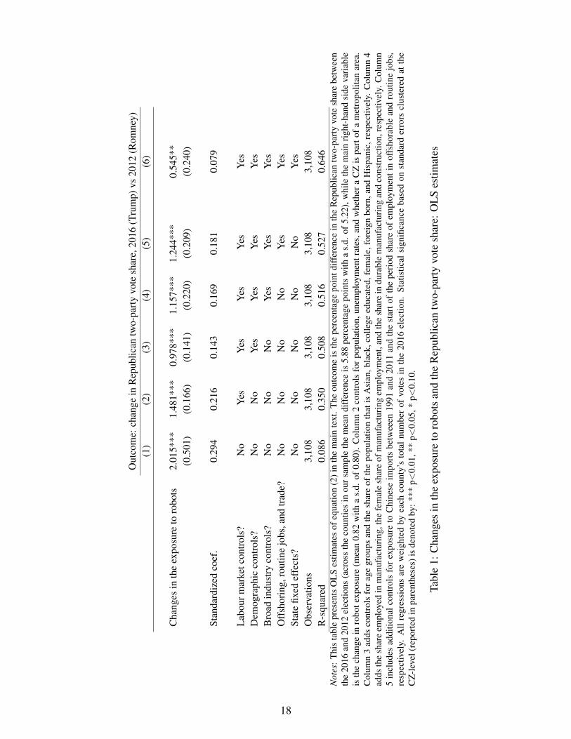
Table 1 presents OLS estimates of equation (2) documenting the positive and highly sta-tistically significant association between changes in robot exposure and changes in the share

17

Out

com

e:ch

ange

inR

epub

lican

two-

part

yvo

tesh

are,

2016

(Tru

mp)

vs20

12(R

omne

y)(1

)(2

)(3

)(4

)(5

)(6

)

Cha

nges

inth

eex

posu

reto

robo

ts2.

015*

**1.

481*

**0.

978*

**1.

157*

**1.

244*

**0.

545*

*(0

.501

)(0

.166

)(0

.141

)(0

.220

)(0

.209

)(0

.240

)

Stan

dard

ized

coef

.0.

294

0.21

60.

143

0.16

90.

181

0.07

9

Lab

ourm

arke

tcon

trol

s?N

oY

esY

esY

esY

esY

esD

emog

raph

icco

ntro

ls?

No

No

Yes

Yes

Yes

Yes

Bro

adin

dust

ryco

ntro

ls?

No

No

No

Yes

Yes

Yes

Off

shor

ing,

rout

ine

jobs

,and

trad

e?N

oN

oN

oN

oY

esY

esSt

ate

fixed

effe

cts?

No

No

No

No

No

Yes

Obs

erva

tions

3,10

83,

108

3,10

83,

108

3,10

83,

108

R-s

quar

ed0.

086

0.35

00.

508

0.51

60.

527

0.64

6N

otes

:T

his

tabl

epr

esen

tsO

LS

estim

ates

ofeq

uatio

n(2

)in

the

mai

nte

xt.T

heou

tcom

eis

the

perc

enta

gepo

intd

iffer

ence

inth

eR

epub

lican

two-

part

yvo

tesh

are

betw

een

the

2016

and

2012

elec

tions

(acr

oss

the

coun

ties

inou

rsa

mpl

eth

em

ean

diff

eren

ceis

5.88

perc

enta

gepo

ints

with

as.

d.of

5.22

),w

hile

the

mai

nri

ght-

hand

side

vari

able

isth

ech

ange

inro

bote

xpos

ure

(mea

n0.

82w

itha

s.d.

of0.

80).

Col

umn

2co

ntro

lsfo

rpo

pula

tion,

unem

ploy

men

trat

es,a

ndw

heth

era

CZ

ispa

rtof

am

etro

polit

anar

ea.

Col

umn

3ad

dsco

ntro

lsfo

rag

egr

oups

and

the

shar

eof

the

popu

latio

nth

atis

Asi

an,b

lack

,col

lege

educ

ated

,fem

ale,

fore

ign

born

,and

His

pani

c,re

spec

tivel

y.C

olum

n4

adds

the

shar

eem

ploy

edin

man

ufac

turi

ng,t

hefe

mal

esh

are

ofm

anuf

actu

ring

empl

oym

ent,

and

the

shar

ein

dura

ble

man

ufac

turi

ngan

dco

nstr

uctio

n,re

spec

tivel

y.C

olum

n5

incl

udes

addi

tiona

lcon

trol

sfo

rex

posu

reto

Chi

nese

impo

rts

betw

eeen

1991

and

2011

and

the

star

tof

the

peri

odsh

are

ofem

ploy

men

tin

offs

hora

ble

and

rout

ine

jobs

,re

spec

tivel

y.A

llre

gres

sion

sar

ew

eigh

ted

byea

chco

unty

’sto

taln

umbe

rof

vote

sin

the

2016

elec

tion.

Stat

istic

alsi

gnifi

canc

eba

sed

onst

anda

rder

rors

clus

tere

dat

the

CZ

-lev

el(r

epor

ted

inpa

rent

hese

s)is

deno

ted

by:*

**p<

0.01

,**

p<0.

05,*

p<0.

10.

Tabl

e1:

Cha

nges

inth

eex

posu

reto

robo

tsan

dth

eR

epub

lican

two-

part

yvo

tesh

are:

OL

Ses

timat

es

18

of votes cast in favour of the Republican candidate. As reflected in the standardized coeffi-cients, a one-standard-deviation increase in the exposure to robots is associated with an 0.294standard-deviation-increase in the Republican two-party vote share (column 1). Put differ-ently, the point estimate of 2.015 implies that if we compare two counties at the 25th and 75thpercentile of robot exposure respectively, the Republican two-party vote share in the countywith a higher level of exposure is predicted to increase by an additional 1.330 percentagepoints in 2016.9 Of course, this bivariate relationship could simply reflect that differences inthe exposure to robots is correlated with a variety of omitted factors: areas with a higher expo-sure to robots also have, for example, lower educational levels, higher initial unemploymentrates, and are more likely to be rural than areas with a lower exposure.

To account for such factors, column 2 adds a set of basic labour market controls. Specif-ically, we control for start-of-the-period differences in population and unemployment rates,as well as whether a CZ is part of a metropolitan area. Because voting patterns are reportedto have varied substantially along a variety of demographic dimensions that also may be cor-related with differences in the exposure to robots, column 3 further adds controls for initialdifferences in age composition of the labour force and the share of the population that isAsian, black, college educated, female, foreign born, and Hispanic, respectively.10 Althoughthe estimated link between robot exposure and an increased vote share for the Republicancandidate declines in magnitude when adding these demographic and labour market controls,it remains sizeable and highly statistically significant.

As the vast majority of robots are used in manufacturing industries, it raises the con-cern that our estimated impacts of robot exposure partly reflect a specialization in industrialwork. In column 4, we further add the start-of-the-period share employed in manufactur-ing, the female share of manufacturing employment, and the share in durable manufacturingand construction, respectively. Along similar lines, the increased exposure to robots may becorrelated with differences across CZs in the exposure to offshoring, routinization, or tradecompetition. Column 5 therefore also adds controls for the start-of-the-period share of thepopulation employed in offshorable and routine jobs following a similar approach in classi-fying occupations as offshorable and routine as Autor and Dorn (2013), as well as the expo-sure of the workforce to Chinese imports between 1991 and 2011 based on data from Autoret al. (2013).11 Notably, the estimates remain similar in magnitude and statistical precisionwhen adding these additional controls, which presumably reflects the considerable variation

9Across the counties in our sample, the 25th and 75th percentile of robot exposure is 0.33 and 0.99 respec-tively that implies an estimated increase in the Republican two-party vote share of 2.015×(0.99−0.33)= 1.330percentage points.

10For brevity we do not report the estimates for these additional covariates, but note that they generally alignwith popular perceptions of the areas that supported Trump: the support was significantly lower, for example, inareas with a more educated population, or where blacks or Hispanics constituted a large share of the population.

11Autor et al. (2016b) and Autor et al. (2016a) further document the impacts of import competition onpolitical polarization in the United States as well as the 2016 presidential election.

19

in robot use within manufacturing and the relatively limited overlap between robot exposureand exposure to Chinese imports, offshoring, and specialization in routine work (Acemogluand Restrepo, 2017). Although the estimated magnitude declines in column 6 when we alsoadd a full set of state fixed effects, thus only exploiting within-state variation, a positive andhighly statistically significant link between changes in the exposure to robots and changesin the Republican two-party vote share persists. Overall, these estimates thus lend strongsupport to the notion that the correlation observed in Figure 1, showing that areas that sawan increasing exposure to robots also were more likely to swing in favour of Trump in the2016 election, does not simply reflect observable differences in, for example, demographicsbetween more and less exposed areas.12

3.3 IV estimates

A central identification challenge is that the exposure to robots may be correlated with avariety of local economic shocks that may in turn have shaped the outcome of the election.While our rich set of controls alleviates some concerns along these lines, it is still possiblethat areas that saw a rising exposure to robots and shifted in favour of Trump at the sametime may have experienced unobserved shocks that we fail to control for. We address suchconcerns by developing two alternative IV strategies. First, we isolate exogenous variation inthe exposure to robot adoption by exploiting historical differences in industrial specializationthat is less likely to correlate with other adverse shocks potentially correlated with differencesin the exposure to robots. To construct our first instrument, we replace the 2011 distribution ofCZ employment with employment shares in 1980 based on census data (Ruggles et al., 2010),which enables us to focus on historical and persistent differences in the specialization of CZsin different industries thus also avoiding any mechanical correlation or mean reversion withchanges in overall or industry-level employment outcomes (Acemoglu and Restrepo, 2017).Using the same notation as above, we thus construct the instrument for each individual CZ j

as:

EIIV 1j = ∑

i∈Ili j,1980× (

RUSi,2015

LUSi,2011

−RUS

i,2011

LUSi,2011

) (3)

A second way to isolate exogenous variation in the exposure to robots across industriesis to exploit cross-industry differences in adoption in countries other than the US, whichapproximates the adoption of robots on the technological frontier. Our second instrument

12An additional concern evident from the distribution of robot exposure depicted in Figure 1 is that ourresults may be sensitive to outliers with the highest level of exposure that also saw the largest increases in theRepublican two-party vote share. Reassuringly, however, excluding the top 1, 2, or 5 per cent of counties interms of their exposure leaves the estimates virtually unchanged both in magnitude and statistical precision (notreported).

20

therefore focuses on variation in robot usage across industries in ten European countries:Austria, Czech Republic, Denmark, Finland, France, Germany, Italy, Spain, Sweden, and theUnited Kingdom. We aggregate the IFR robot data to be compatible with the EU KLEMSindustrial employment data (Jager, 2016), which yields 16 industries based on ISIC Rev 4that requires us to also map the US employment composition to this industrial structure.13

We then construct the second instrument for each CZ j as follows:

EIIV 2j = ∑

i∈Ili j,1980× (mean(

Ri,2015

Li,2011)−mean(

Ri,2011

Li,2011)) (4)

where mean(Ri,tLi,t

) denotes the average robot usage among European countries in industry i

and year t, and li j,1980 corresponds to the 1980 share of a CZ’s j employment in industryi. The variation in the instrument is thus derived from historical differences in industrialspecialization across CZs and changes in average robot use in industries in countries outsideof the United States.

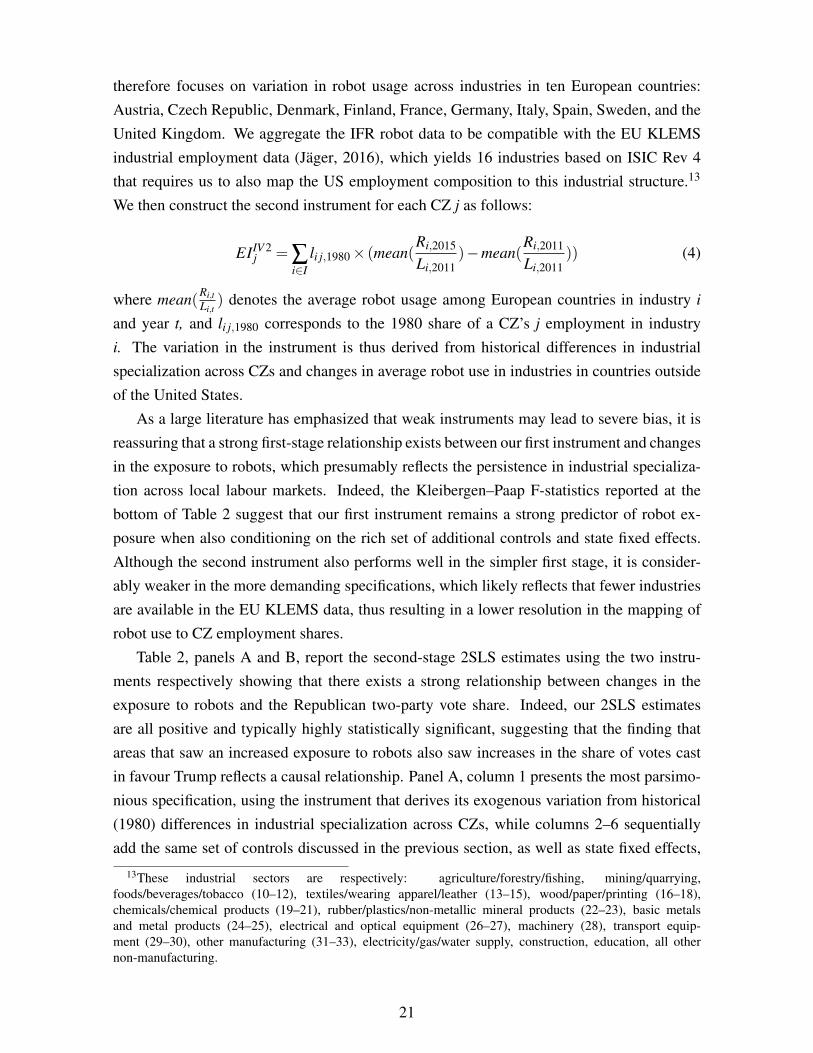
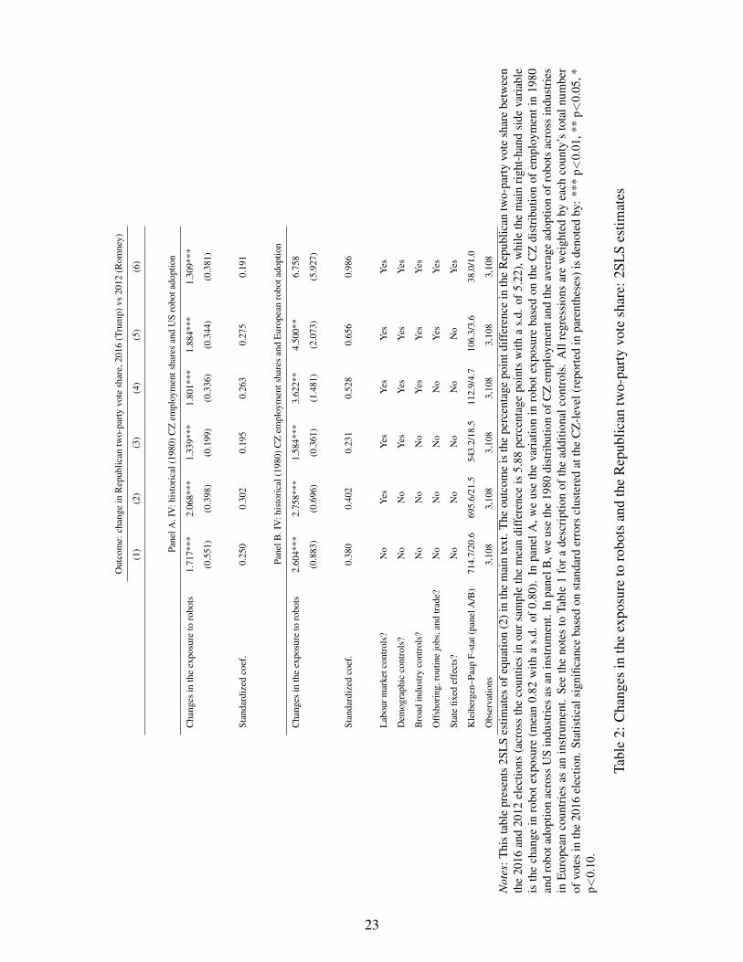
As a large literature has emphasized that weak instruments may lead to severe bias, it isreassuring that a strong first-stage relationship exists between our first instrument and changesin the exposure to robots, which presumably reflects the persistence in industrial specializa-tion across local labour markets. Indeed, the Kleibergen–Paap F-statistics reported at thebottom of Table 2 suggest that our first instrument remains a strong predictor of robot ex-posure when also conditioning on the rich set of additional controls and state fixed effects.Although the second instrument also performs well in the simpler first stage, it is consider-ably weaker in the more demanding specifications, which likely reflects that fewer industriesare available in the EU KLEMS data, thus resulting in a lower resolution in the mapping ofrobot use to CZ employment shares.

Table 2, panels A and B, report the second-stage 2SLS estimates using the two instru-ments respectively showing that there exists a strong relationship between changes in theexposure to robots and the Republican two-party vote share. Indeed, our 2SLS estimatesare all positive and typically highly statistically significant, suggesting that the finding thatareas that saw an increased exposure to robots also saw increases in the share of votes castin favour Trump reflects a causal relationship. Panel A, column 1 presents the most parsimo-nious specification, using the instrument that derives its exogenous variation from historical(1980) differences in industrial specialization across CZs, while columns 2–6 sequentiallyadd the same set of controls discussed in the previous section, as well as state fixed effects,

13These industrial sectors are respectively: agriculture/forestry/fishing, mining/quarrying,foods/beverages/tobacco (10–12), textiles/wearing apparel/leather (13–15), wood/paper/printing (16–18),chemicals/chemical products (19–21), rubber/plastics/non-metallic mineral products (22–23), basic metalsand metal products (24–25), electrical and optical equipment (26–27), machinery (28), transport equip-ment (29–30), other manufacturing (31–33), electricity/gas/water supply, construction, education, all othernon-manufacturing.

21

respectively. As shown in these estimates, the positive relationship between changes in theexposure to robots and changes in the Republican two-party vote share persists and suggeststhat a one-standard-deviation increase in robot exposure leads to an 0.191-standard-deviationincrease in the share of votes cast for Trump (column 6). Panel B presents 2SLS estimatesfrom similar specifications, instead using the alternative instrument in the first stage, whichderives its exogenous variation in robot exposure from historical differences in industrial spe-cialization across CZs and the average rate of robot adoption across industries in Europeancountries. Although these results should be interpreted somewhat more carefully, given thatthe instrument is a less strong predictor of differences in exposure in the more extensivespecifications, it is reassuring that the second-stage estimates consistently return a positiveand generally statistically significant link between changes in robot exposure and changes inthe Republican two-party vote share that are broadly in line with the estimates reported inpanel A.

Together, these results show that the correlations documented in the previous section areplausibly causal and that the simple correlation between robot exposure and the support forTrump, if anything, is likely to understate the effects of robots on the 2016 presidential elec-tion. Yet, while the finding that electoral districts that became more exposed to automationduring the years running up to the election were more likely to vote for Trump is an inter-esting and important result in itself, it does not shed light on the extent to which this impactshaped the outcome of the election.

3.4 Did robots swing the 2016 US presidential election?

While the above-reported results document a direct positive link between changes in theexposure to robots and the support for the Republican candidate in the 2016 election, they donot shed light on whether the outcome of the election would have changed in a counterfactualscenario with a lower penetration of robots. We next provide such a counterfactual exercise,showing that if the exposure to robots had not increased in the years running up to the vote,the election would have swung in favour of the Democratic candidate.

To examine how the outcome of the 2016 election would have changed if the pace ofrobot adoption had slowed down, we perform a variety of counterfactual estimates based onour most conservative and preferred IV estimate in column 6 of Table 2, panel A, whichindicates that Trump gained on average 1.309 percentage points of the two-party vote sharefor each unit increase in the exposure to robots in a county. Using this estimate, we firstcompute the share of the two-party vote that the Republican candidate would have lost if theexposure to robots had been Y per cent smaller, as 1.309× (Y %×EI j) for each county inour sample. Then, we multiply this share with the number of two-party votes in each countyto obtain the number of votes that Trump would have lost to Clinton in the counterfactual

22

Out

com

e:ch

ange

inR

epub

lican

two-

part

yvo

tesh

are,

2016

(Tru

mp)

vs20

12(R

omne

y)

(1)

(2)

(3)

(4)

(5)

(6)

Pane

lA.I

V:h

isto

rica

l(19

80)C

Zem

ploy

men

tsha

res

and

US

robo

tado

ptio

n

Cha

nges

inth

eex

posu

reto

robo

ts1.

717*

**2.

068*

**1.

339*

**1.

801*

**1.

884*

**1.

309*

**

(0.5

51)

(0.3

98)

(0.1

99)

(0.3

36)

(0.3

44)

(0.3

81)

Stan

dard

ized

coef

.0.

250

0.30

20.

195

0.26

30.

275

0.19

1

Pane

lB.I

V:h

isto

rica

l(19

80)C

Zem

ploy

men

tsha

res

and

Eur

opea

nro

bota

dopt

ion

Cha

nges

inth

eex

posu

reto

robo

ts2.

604*

**2.

758*

**1.

584*

**3.

622*

*4.

500*

*6.

758

(0.8

83)

(0.6

96)

(0.3

61)

(1.4

81)

(2.0

73)

(5.9

27)

Stan

dard

ized

coef

.0.

380

0.40

20.

231

0.52

80.

656

0.98

6

Lab

ourm

arke

tcon

trol

s?N

oY

esY

esY

esY

esY

es

Dem

ogra

phic

cont

rols

?N

oN

oY

esY

esY

esY

es

Bro

adin

dust

ryco

ntro

ls?

No

No

No

Yes

Yes

Yes

Off

shor

ing,

rout

ine

jobs

,and

trad

e?N

oN

oN

oN

oY

esY

es

Stat

efix

edef

fect

s?N

oN

oN

oN

oN

oY

es

Kle

iber

gen–

Paap

F-st

at(p

anel

A/B

)71

4.7/

20.6

695.

6/21

.554

3.2/

18.5

112.

9/4.

710

6.3/

3.6

38.0

/1.0

Obs

erva

tions

3,10

83,

108

3,10

83,

108

3,10

83,

108

Not

es:T

his

tabl

epr

esen

ts2S

LS

estim

ates

ofeq

uatio

n(2

)in

the

mai

nte

xt.T

heou

tcom

eis

the

perc

enta

gepo

intd

iffer

ence

inth

eR

epub

lican

two-

part

yvo

tesh

are

betw

een

the

2016

and

2012

elec

tions

(acr

oss

the

coun

ties

inou

rsa

mpl

eth

em

ean

diff

eren

ceis

5.88

perc

enta

gepo

ints

with

as.

d.of

5.22

),w

hile

the

mai

nri

ght-

hand

side

vari

able

isth

ech

ange

inro

bote

xpos

ure

(mea

n0.

82w

itha

s.d.

of0.

80).

Inpa

nelA

,we

use

the

vari

atio

nin

robo

texp

osur

eba

sed

onth

eC

Zdi

stri

butio

nof

empl

oym

enti

n19

80an

dro

bota

dopt

ion

acro

ssU

Sin

dust

ries

asan

inst

rum

ent.

Inpa

nelB

,we

use

the

1980

dist

ribu

tion

ofC

Zem

ploy

men

tand

the

aver

age

adop

tion

ofro

bots

acro

ssin

dust

ries

inE

urop

ean

coun

trie

sas

anin

stru

men

t.Se

eth

eno

tes

toTa

ble

1fo

ra

desc

ript

ion

ofth

ead

ditio

nalc

ontr

ols.

All

regr

essi

ons

are

wei

ghte

dby

each

coun

ty’s

tota

lnum

ber

ofvo

tes

inth

e20

16el

ectio

n.St

atis

tical

sign

ifica

nce

base

don

stan

dard

erro

rscl

uste

red

atth

eC

Z-l

evel

(rep

orte

din

pare

nthe

ses)

isde

note

dby

:**

*p<

0.01

,**

p<0.

05,*

p<0.

10.

Tabl

e2:

Cha

nges

inth

eex

posu

reto

robo

tsan

dth

eR

epub

lican

two-

part

yvo

tesh

are:

2SL

Ses

timat

es

23

scenario of lower robot exposure. Lastly, we aggregate the counterfactual county vote totalswithin each state and allocate the implied electoral votes to identify the victor.

Table 3 reports results from this exercise, showing the winner and the vote margin infavour of Trump in a set of closely contested states and aggregate changes in the electoralvotes going to Trump and Clinton, respectively, under different counterfactual scenarios ofrobot exposure had it been 10, 75, or 95 per cent lower. Already at a 10 per cent lower robotexposure, our estimates predict that Michigan would have swung in favour of the Democraticcandidate, whereas in a scenario where the use of robots virtually did not increase in the yearsleading up to the election (i.e. with a 95 per cent lower exposure) Trump would additionallyhave lost both Pennsylvania and Wisconsin, thus leaving Clinton with a majority in the Elec-toral College. While this counterfactual exercise naturally should be interpreted carefully, itdoes suggest that automation had potentially pervasive effects on the outcomes of the 2016election as it had severe impacts in several contested states.

4 Concluding remarks

The politics of automation has shaped our economic trajectories for millennia. Prior to the‘great escape’ brought by the Industrial Revolution, political leaders frequently banned anylabour-saving technology for fear of social unrest, providing one explanation for why eco-nomic growth was stagnant for most of human history (Acemoglu and Robinson, 2013;Mokyr, 1990). The British government was the first to consistently and vigorously takeaction against any attempts to hinder the spread of machines, offering ‘another explanationwhy Britain’s Industrial Revolution was first’ (Mokyr, 1992). The long-term benefits of theIndustrial Revolution have been immense and indisputable: prior to 1750, per capita incomesin the world doubled every 6,000 years; thereafter, it has taken some 50 years for incomes todouble (DeLong, 1998). Even the poorest British citizens today enjoy goods and services inan abundance that was unimaginable to their pre-industrial ancestors. But those benefits cameat the expense of three generations of Englishmen (see Figure 2), of whom many were madeworse off by the force of technology (Shaw-Taylor and Jones, 2010; Allen, 2016; Baines,1835; Allen, 2009).14 To borrow David Landes (2003) phrase:

if mechanization opened new vistas of comfort and prosperity for all men, it alsodestroyed the livelihood of some and left others to vegetate in the backwaters ofthe stream of progress. [...] the victims of the Industrial Revolution numbered inthe hundreds of thousands or even millions.

14Thus, economic historians have long debated if the Industrial Revolution was ‘worth it’ (see Williamson,1982).

24

Cou

nter

fact

ualo

utco

mes

due

toa

low

erex

posu

reto

robo

tsA

ctua

lout

com

eof

2016

elec

tion

10%

low

er75

%lo

wer

95%

low

erW

inne

rM

argi

n(#

vote

s)M

argi

n(%

ofvo

tes)

Win

ner

Mar

gin

(%)

Win

ner

Mar

gin

(%)

Win

ner

Mar

gin

(%)

Geo

rgia

Rep

ublic

an21

1,14

15.

10R

epub

lican

5.03

Rep

ublic

an4.

57R

epub

lican

4.42

Ari

zona

Rep

ublic

an91

,234

3.50

Rep

ublic

an3.

46R

epub

lican

3.18

Rep

ublic

an3.

10N

orth

Car

olin

aR

epub

lican

173,

315

3.66

Rep

ublic

an3.

57R

epub

lican

3.01

Rep

ublic

an2.

83Fl

orid

aR

epub

lican

112,

911

1.19

Rep

ublic

an1.

16R

epub

lican

0.96

Rep

ublic

an0.

90Pe

nnsy

lvan

iaR

epub

lican

44,2

920.

72R

epub

lican

0.64

Rep

ublic

an0.

15D

emoc

rat

-0.0

1W

isco

nsin

Rep

ublic

an22

,748

0.76

Rep

ublic

an0.

66D

emoc

rat

–0.0

5D

emoc

rat

-0.2

6M

ichi

gan

Rep

ublic

an10

,704

0.22

Dem

ocra

t-0

.20

Dem

ocra

t–2

.92

Dem

ocra

t-3

.75

New

Ham

pshi

reD

emoc

rat

–2,7

36–0

.37

Dem

ocra

t-0

.44

Dem

ocra

t–0

.92

Dem

ocra

t-1

.06

Min

neso

taD

emoc

rat

–44,

593

–1.5

1D

emoc

rat

-1.6

0D

emoc

rat

–2.1

3D

emoc

rat

-2.3

0

Ele

ctor

alvo

tes

Trum

p30

629

028

026

0E

lect

oral

vote

sC

linto

n23

224

825

827

8N

otes

:T

his

tabl

epr

esen

tsth

ew

inne

ran

dth

evo

tem

argi

nin

favo

urof

the

Rep

ublic

anca

ndid

ate

inth

e20

16el

ectio

nin

ase

tof

clos

ely

cont

este

dst

ates

and

inte

rms

ofto

tale

lect

oral

vote

s,as

wel

las

coun

terf

actu

alou

tcom

esw

here

we

estim

ate

how

stat

e-le

velv

otin

gou

tcom

esw

ould

have

chan

ged

ina

scen

ario

with

low

erle

vels

ofro

bot

expo

sure

base

don

oure

stim

ate

inco

lum

n6

ofTa

ble

2,pa

nelA

.See

the

mai

nte

xtfo

rafu

rthe

rdis

cuss

ion

ofth

ese

estim

ates

.

Tabl

e3:

Cou

nter

fact

ualo

utco

mes

incl

osel

yco

ntes

ted

stat

esan

dth

e20

16el

ectio

n

25

Could the British Industrial Revolution have happened if ordinary workers were also voters?Of course, there is no way of running the experiment, but many did their utmost to bring thespread of machines to a halt by the means they had: besides the flood of petitions againstmachines that came into parliament, workers voted against machines with sticks and stones(Mantoux, 2013).15 As an analogy, Wassily Leontief famously suggested that, “If horsescould have joined the Democratic party and voted, what happened on farms might have beendifferent.”16 Instead, the proliferation of automobiles, tractors, and trucks caused the anni-hilation of the horse as a prime mover on farms and as a mean of moving goods and peoplearound. While the robot revolution has not rendered the workforce redundant, many Amer-icans have lost the race to technology, which is reflected in the reallocation of millions ofworkers from middle-income jobs to low-income occupations or non-employment as theirjobs have been automated away (Autor and Dorn, 2013; Cortes et al., 2016a; Acemoglu andRestrepo, 2017). This paper has shown that the victims of the robot revolution have a higherpropensity to opt for radical political change by providing evidence that electoral districtswith higher exposure to robots were significantly more likely to support Trump.

Looking forward, automation is likely to become a growing political challenge.17 The po-tential scope of automation now extends well beyond industrial robots. Recent developmentsin artificial intelligence and mobile robotics are widely regarded the beginnings of a ‘SecondMachine Age’; machines are now able to perform even a wider range of non-routine tasks,such as medical diagnostics, translation work, and driving a car (Brynjolfsson and McAfee,2014). As a result, Frey and Osborne (2017) estimate that 47 per cent of US employment is at‘high risk’ of automation over the forthcoming decades, with a substantial share falling intonon-tradable sectors of the economy, to which most workers have already reallocated: 98 percent of total US employment growth between 1990 and 2008 accrued in sectors where jobsare unaffected by import competition (Spence and Hlatshwayo, 2012). While this shieldsmany workers from the adverse impacts of trade (Acemoglu et al., 2016), it does not consti-tute a safeguard against automation—indeed, as President Obama noted when leaving office:‘The next wave of economic dislocations won’t come from overseas. It will come from therelentless pace of automation that makes a lot of good, middle-class jobs obsolete.’

Of course, over the very long run automation has always been an engine of comfort andprosperity. After six decades of stagnant wage growth during the British Industrial Revo-lution, ordinary workers eventually became the prime beneficiaries of automation as theyadapted and acquired new skills (Galor and Moav, 2004; Bessen, 2015). Between 1840 and

15Most citizens lacked voting rights, for which property ownership remained a prerequisite; even with theReform Acts of 1832 and 1867.

16Cited in Curtis (1983).17As forcefully argued by Crafts (2015), ‘fears about long-term “secular stagnation”, based on the end of

innovation as we have known it, seem overdone. The problem is much more likely to be the factor-saving biasof technological progress based on computerization of jobs than a drying-up of productivity growth.’

26

1900, real wages in Britain grew by 123 per cent, considerably faster than output per worker(Allen, 2009). Could history repeat itself? Perhaps so; so far, the economic trajectories ofthe age of automation closely resembles those of the British Industrial Revolution. But anyfuture benefits from automation hinge upon its politics. To avoid further populist rebellionand a looming backlash against technology itself, governments must find ways of making thebenefits from automation more widely shared.

References

Acemoglu, D. (2002). Technical change, inequality, and the labor market. Journal of Eco-

nomic Literature, 40(1), 7–72.

Acemoglu, D. and Autor, D. (2011). Skills, tasks and technologies: Implications for employ-ment and earnings. Handbook of labor economics, 4, 1043–1171.

Acemoglu, D. and Restrepo, P. (2017). Robots and Jobs: Evidence from US labor markets.

Acemoglu, D. and Robinson, J. A. (2013). Why nations fail: The origins of power, prosperity,

and poverty. Crown Business.

Acemoglu, D., Autor, D., Dorn, D., Hanson, G. H., and Price, B. (2016). Import competitionand the great U.S. employment sag of the 2000s. Journal of Labor Economics, 34(S1),S141–S198.

Akst, D. (2013). What can we learn from past anxiety over automation? The Wilson Quar-

terly.

Allen, R. (2016). The hand-loom weaver and the power loom: A schumpeterian perspective.Technical report, University of Oxford, Department of Economics.

Allen, R. C. (2005). English and Welsh agriculture, 1300-1850: outputs, inputs, and income.

Allen, R. C. (2009). Engels pause: Technical change, capital accumulation, and inequality inthe British industrial revolution. Explorations in Economic History, 46(4), 418–435.

Autor, D., Levy, F., and Murnane, R. J. (2003). The skill content of recent technologicalchange: An empirical exploration. The Quarterly Journal of Economics, 118(4), 1279–1333.

Autor, D., Dorn, D., Hanson, G., and Majlesi, K. (2016a). Importing political polarization?The electoral consequences of rising trade exposure. Technical report, National Bureau ofEconomic Research.

27

Autor, D., Dorn, D., Hanson, G., and Majlesi, K. (2016b). A note on the effect of rising tradeexposure on the 2016 presidential election. Technical report, Mimeo, MIT.

Autor, D. H. and Dorn, D. (2013). The Growth of Low-Skill Service Jobs and the Polarizationof the U.S. Labor Market. American Economic Review, 103(5), 1553–97.

Autor, D. H., Katz, L. F., and Kearney, M. S. (2006). The Polarization of the U.S. LaborMarket. American Economic Review, 96(2), 189–194.

Autor, David, H., Dorn, D., and Hanson, G. H. (2013). The China syndrome: Local labormarket effects of import competition in the United States. The American Economic Review,103(6), 2121–2168.

Baines, E. (1835). History of the Cotton Manufacture in Great Britain. Londres, Fischer and

Jackson.

Berg, M. (1982). The machinery question and the making of political economy 1815-1848.Technical report, Cambridge University Press.

Berger, T. and Frey, C. B. (2016). Did the Computer Revolution shift the fortunes of U.S.cities? Technology shocks and the geography of new jobs. Regional Science and Urban

Economics, 57, 38–45.

Berger, T. and Frey, C. B. (2017). Industrial renewal in the 21st century: evidence from UScities. Regional Studies, 51(3), 404–413.

Bessen, J. (2015). Learning by doing: the real connection between innovation, wages, and

wealth. Yale University Press.

Bivens, J., Gould, E., Mishel, E., and Shierholz, H. (2014). Raising Americas Pay. Economic

Policy Institute Briefing Paper, 378.

Brynjolfsson, E. and McAfee, A. (2014). The second machine age: Work, progress, and

prosperity in a time of brilliant technologies. WW Norton & Company.

Caprettini, B. and Voth, H.-J. (2017). Rage Against the Machines: Labour-Saving Technol-ogy and Unrest in England, 1830-32.

Clark, G. (2005). The condition of the working class in England, 1209–2004. Journal of

Political Economy, 113(6), 1307–1340.

Cortes, G. M., Jaimovich, N., and Siu, H. E. (2016a). Disappearing routine jobs: Who, how,and why? Technical report, National Bureau of Economic Research.

28

Cortes, G. M., Jaimovich, N., and Siu, H. E. (2016b). The end of men and rise of women inthe high-skilled labor market.

Crafts, N. (2015). Economic growth: onwards and upwards? Oxford Review of Economic

Policy, 31(2), 217–241.

Crafts, N. F. and Harley, C. K. (1992). Output growth and the British industrial revolution: arestatement of the Crafts-Harley view. The Economic History Review, 45(4), 703–730.

Curtis, C. (1983). Machines vs. workers. The New York Times.

David, H. (2015). Why are there still so many jobs? the history and future of workplaceautomation. The Journal of Economic Perspectives, 29(3), 3–30.

DeLong, J. B. (1998). Estimating world GDP, one million BC–present. Berkeley, California.

Eberstadt, N. (2016). Men Without Work: America’s Invisible Crisis. Templeton FoundationPress.

Engels, F. (1845). The Condition of the Working Class in England. Collected Works. London:

Lawrence & Wishart, page 4.

Feinstein, C. H. (1998). Pessimism perpetuated: real wages and the standard of living inBritain during and after the industrial revolution. The Journal of Economic History, 58(3),625–658.

Floud, R., Gregory, A., and Wachter, K. (1990). Height, health and history: nutritional status

in the United Kingdom, 1750-1980. Number 9. Cambridge University Press.

Frey, C. B. and Osborne, M. A. (2017). The future of employment: how susceptible are jobsto computerisation? Technological Forecasting and Social Change, 114, 254–280.

Galor, O. and Moav, O. (2004). From physical to human capital accumulation: Inequalityand the process of development. The Review of Economic Studies, 71(4), 1001–1026.

Goos, M. and Manning, A. (2007). Lousy and lovely jobs: The rising polarization of workin Britain. The Review of Economics and Statistics, 89(1), 118–133.

Goos, M., Manning, A., and Salomons, A. (2009). Job polarization in Europe. The American

Economic Review, 99(2), 58–63.

Goos, M., Manning, A., and Salomons, A. (2014). Explaining job polarization: Routine-biased technological change and offshoring. The American Economic Review, 104(8),2509–2526.

29

Gordon, R. J. (2016). The rise and fall of American growth: The US standard of living since

the civil war. Princeton University Press.

Graetz, G. and Michaels, G. (2015). Robots at work. CEP Discussion Paper No 1335.

Hamel, L., Firth, J., and Brodie, M. (2014). Kaiser Family Foundation/New York Times/CBSNews Non-Employed Poll.

Horrell, S. (1996). Home demand and british industrialization. The Journal of Economic

History, 56(3), 561–604.

Jager, K. (2016). Eu klems growth and productivity accounts 2016 release, statistical mod-ule1.

Jaimovich, N. and Siu, H. E. (2012). Job polarization and jobless recoveries. NBER Working

Paper 18334.

Karabarbounis, L. and Neiman, B. (2013). The global decline of the labor share. The Quar-

terly Journal of Economics, 129(1), 61–103.

Katz, L. F. and Murphy, K. M. (1992). Changes in relative wages, 1963–1987: supply anddemand factors. The Quarterly Journal of Economics, 107(1), 35–78.

Komlos, J. (1998). Shrinking in a growing economy? the mystery of physical stature duringthe industrial revolution. The Journal of Economic History, 58(3), 779–802.

Landes, D. S. (2003). The unbound Prometheus: technological change and industrial devel-

opment in Western Europe from 1750 to the present. Cambridge University Press.

Lindert, P. H. (2000). When did inequality rise in Britain and America? Journal of Income

Distribution, 9(1), 11–25.

Lindert, P. H. and Williamson, J. G. (1983). The Economic History Review, 36(1), 1–25.

Lindert, P. H. and Williamson, J. G. (2016). Unequal Gains: American Growth and Inequality

since 1700. Princeton University Press.

Mantoux, P. (2013). The industrial revolution in the eighteenth century: An outline of the

beginnings of the modern factory system in England. Routledge.

Michaels, G., Natraj, A., and Reenen, J. V. (2014). Has ICT Polarized Skill Demand? Ev-idence from Eleven Countries over Twenty-Five Years. The Review of Economics and

Statistics, 96(1), 60–77.

30

Mokyr, J. (1990). The lever of riches: Technological creativity and economic progress. Ox-ford University Press.

Mokyr, J. (1992). Technological inertia in economic history. The Journal of Economic

History, 52(2), 325–338.

Mokyr, J. (1998). The Political Economy of Technological Change: Resistance and Innova-

tion in Economic History, pages 39–64. Edward Elgar Publishers.

Mokyr, J. (2009). The Enlightened Economy: An Economic History of Britain 1700-1850.Yale University Press.

Mokyr, J., Vickers, C., and Ziebarth, N. L. (2015). The history of technological anxietyand the future of economic growth: Is this time different? The Journal of Economic

Perspectives, 29(3), 31–50.

Nordhaus, W. D. (2007). Two centuries of productivity growth in computing. The Journal of

Economic History, 67(01), 128–159.

Pew Research Center (2017). Automation in everyday life.

Ruggles, S., Alexander, J. T., Genadek, K., Goeken, R., Schroeder, M. B., and Sobek,M. (2010). Integrated public use microdata series: Version 5.0 (machine-readabledatabase). minneapolis: University of minnesota, 2006 american community survey. rug-gles2010integrated.

Shaw-Taylor, L. and Jones, A. (2010). The male occupational structure of Northamptonshire1777-1881: A case of partial de-industrialization? Cambridge University Working Paper,5.

Spence, M. and Hlatshwayo, S. (2012). The evolving structure of the American economyand the employment challenge. Comparative Economic Studies, 54(4), 703–738.

Summers, L. (2015). Focus on growth for the middle class. The Washington Post.

Tuttle, C. (1999). Hard at work in factories and mines: the economics of child labor during

the British industrial revolution. Westview Press.

Ure, A. (1835). The Philosophy of Manufactures; or, An Exposition of the Scientific, Moral,

and Commercial Economy of the Factory System of Great Britain. C. Knight.

Voth, H.-J. (2000). Time and work in England 1750-1830. Clarendon Press Oxford.

Williamson, J. G. (1982). Was the industrial revolution worth it? Disamenities and death in19th century British towns. Explorations in Economic History, 19(3), 221–245.

31