Politics in the FamilyNepotism and the Hiring Decisions of Italian Firms∗

Stefano GagliarducciUniversity of Tor Vergata and EIEF

Marco ManacordaQueen Mary University of London, CEP (LSE) and CEPR

December 2017

Abstract

In this paper we study the effect of family connections to politicians on individuals’labor market outcomes. Using data for Italy spanning over three decades on a sampleof almost one million working age individuals plus data on the universe of individualsholding political office, we estimate that, while in office, an average politician is able toextract around 9,000 euros worth of private sector earnings per year for his close familymembers. We present evidence consistent with the hypothesis that this is a form ofcorruption, i.e., based on a quid-pro-quo exchange between employers and politicians,although an inferior substitute for easier to detect modes of rent appropriation on thepart of politicians.

JEL codes: D72, D73, H72, J24, J30, M51.Keywords: Nepotism, Family connections, Politics, Corruption.

∗We are grateful to Stephane Bonhomme, David Card and Ray Fisman for very useful discussions, and to seminar partici-

pants at the Bank of Italy, Berkeley, Bocconi, Cagliari, CEMFI, Collegio Carlo Alberto, EIEF, EUI, Goteborg, HEC Montreal,

Munich, LSE, Padua, UPF, Tel Aviv, the CEPR Public Economics Annual Symposium, the RIDGE/LACEA-PEG Workshop

on Political Economy and the Festival dell’Economia di Trento for many useful comments. Access to INPS data was performed

in a secure lab environment: we are extremely grateful to Tito Boeri for facilitating access and to Leda Accosta, Cinzia Ferrara

and Giulio Mattioni for their invaluable help with the data. We are also grateful to Luigi Guiso, Paolo Pinotti and Bruno Pel-

legrino for sharing some of the data used in this paper. Lorenzo Ferrari provided excellent research assistantship. Gagliarducci

gratefully acknowledges financial assistance from UniCredit & Universities Foundation under a Modigliani Research Grant. Ste-

fano Gagliarducci: stefano.gagliarducci@uniroma2.it; Department of Economics and Finance, Universita di Roma Tor Vergata,

Via Columbia 2, 00133 Rome (Italy). Marco Manacorda: m.manacorda@qmul.ac.uk; School of Economics and Finance, Queen

Mary University of London, Mile End Road, London E1 4NS (UK).

1

1 Introduction

This paper combines micro data for Italy over almost thirty years on the universe of around

500,000 individuals holding political office with micro data on a random sample of almost

one million working age individuals to estimate the returns - in terms of private sector

jobs among family members - to holding political office. We present an array of evidence

consistent with the view that the phenomenon we uncover is a form of corruption, i.e., based

on a quid-pro-quo exchange between firms and politicians. We argue that nepotism is akin

to - although arguably an inferior substitute for - sheer corruption.

There is plenty of anecdotal evidence that private firms often reserve special treatment to

politicians’ family members, including in what are typically regarded more mature democra-

cies. The argument goes that in exchange for, or in expectation of, political favors, firms hire

or promote politicians’ relatives or grant them higher earnings.1 Evidence though remains

elusive. We bring this argument to empirical scrutiny using data from Italy and investigate

the main determinants and correlates of this phenomenon.

Italy appears an ideal case study for our analysis. The roles of family ties and the lack of

trust, civic participation and meritocracy in shaping the fabric of society and the economy

have been long recognized, and often seen the root of the country’s inability to modernize

(Banfield 1958, Pellegrino and Zingales 2014, Putnam et al 1993). Alongside, widespread

red tape and a cumbersome bureaucracy create opportunities for corruption and politicians’

personal enrichment, with the country ranking third from the bottom among OECD high-

income countries in the Ease of Doing Business index (World Bank 2014) and highest among

all European countries on the Corruption Perceptions index (Transparency International

2014).

One major advantage of the data that we have assembled is that they provide information

on each individual’s tax code, which in Italy includes the First Three Consonants (in short

F3C) of one’s last name and an identifier for the municipality of birth. We identify “families”

based on individuals sharing the same F3C and born in the same municipality.

In order to identify the effect of a family member holding office on individuals’ labor

market outcomes we exploit the longitudinal nature of the data and the timing of family

members’ movements in and out of office. In practice, we compare changes in labor market

1 Allegations of political nepotism against companies often surface in the press, including in the USA. Oneprominent recent case involves the SEC’s allegations that “JPMorgan’s [...] hired the children of high-rankingChinese officials to help win business (Financial Times 2015).

2

outcomes among individuals whose family members enter or leave office to changes in labor

market outcomes among otherwise similar individuals who do not experience such entry or

exit. Based on this strategy, we find positive and precisely estimated effects of a family

member in office on both earnings and months of work.

As one might be legitimately concerned that families’ movements in and out of office and

labor market fortunes might be spuriously correlated, we present an array of evidence to

corroborate our claim that the effects we uncover are causal. First, we use an event-study

analysis to show that there are no pre-trends in labor market outcomes prior to a family

member taking office and that the effect manifests precisely in the year in which this family

member takes office, and tends to fade out as the end of the mandate approaches. Second, we

show that our results remain unchanged when we restrict the estimation sample to individuals

who, at one point over the period of analysis, have a family member in office. In this way, we

rely only on the variation in the timing of entry into and exit from office for identification.

This somewhat tempers the concern that we compare families with very different latent

trends in the variables of interest. Third, we include in the model the interaction between

individual fixed effects and time effects. In this model we identify the effect of connections

net of underlying family specific time effects in both individuals’ labor market fortunes and

in the probability of assuming office. Identification here is extremely demanding as it relies

on highly temporally localized changes in the variables of interest. Our results are robust to

all these checks.

Despite the very fine-grained partition of the data, our matching method identifies fami-

lies with error, since not only does it fail to classify some connected individuals (those with

a different F3C) as family members but - more importantly - it erroneously classifies some

unconnected individuals (those with the same F3C) as family members. Clearly, this is not

a problem unique to our approach, as several other papers that use last names to identify

family connections (reviewed below) suffer from a similar problem. Although one might

be concerned that using F3Cs as opposed to last names makes the problem much worse,

we claim that - whether one uses F3Cs or last names to identify family connections - mis-

classification will occur and we show that this induces a systematic downward bias in our

estimates. We also show that one can use information on the distribution of F3Cs in the

sample to correct the estimates for this source of non-systematic measurement error.

Our estimates imply that individuals in office generate on average extra 9,000 euros

3

worth of private sector earnings among their family members carrying the same last name

and born in the same municipality. These are likely to be conservative estimates of the

returns to holding office in terms of family earnings, as they exclude family members with

different last names or born elsewhere.

In the second part of the paper, we bring ammunition to the argument that our estimates

capture corrupt practices by examining the gradient in the estimated effects as a function of

politicians’ clout. If the effect we find is due to rent extraction on the part of politicians, one

will expect this effect to be larger the larger the rents accruing to office. Consistent with this,

we find that the estimated effect is larger the higher the level of political office (executive

versus legislative branch), the higher the level of government (regional versus municipal),

and the longer the tenure in office. Similar to Brollo et al (2013) and Dal Bo et al’s (2006)

claim that corruption increases when resources increase, we also find that the effect is larger

the larger the budget available to the administration where the politician serves. Effects

are also larger in sectors that are more dependent on the public administration, where the

returns to nepotistic hiring are presumably higher.

We finally investigate how nepotistic hiring varies with the cost of alternative technologies

of rent extraction on the part of politicians. Although grafting or the extraction of monetary

bribes might be cost-effective ways for politicians to monetize over the rents that accrue to

office, these are clearly more easily detectable than having one’s family members hired by a

firm. If disclosed, payment of bribes will also entail costs for the corruptor, as this is evidence

of misbehavior, while per se the hiring of a politician’s family member is not. A corollary

to this assertion is that, if the cost of these alternative technologies of rent appropriation

increases, one will expect parties to shift towards more hidden, harder-to-detect forms of

corruption.

In the final part of the paper we bring this argument to empirical scrutiny by exploiting

the heterogeneous effect across judicial districts of a major anti-corruption campaign,“Mani

Pulite” (literally “Clean Hands”), that swept Italy in the early 1990s and that entailed an

aggressive prosecution of firms and politicians involved in payment and receipt of mone-

tary bribes. The campaign eventually led to the collapse of traditional political parties and

the overall system of representation that had emerged in post-war Italy. Historiographi-

cal accounts of this campaign suggest that this was initiated and supported by judges and

prosecutors with close links to Magistratura Democratica, the left-wing faction of the Associ-

4

azione Nazionale Magistrati (the association of Italian judges and prosecutors). We compare

changes in corruption cases prosecuted in each of the 26 judicial districts before (1985-1991)

and after (1992-2011) “Mani Pulite”. Consistent with increased deterrence, we find a smaller

increase in the number of corruption cases in offices with a greater baseline share of judges

and prosecutors affiliated with Magistratura Democratica. However, we also find a greater

increase in the spread of nepotistic hiring in these areas. We take this evidence to suggest

that nepotistic hiring is a substitute - and potentially an inferior one - for grafting and mon-

etary bribes. Our result is reminiscent of Olken’s (2007) finding that increased corruption

monitoring in Indonesia leads to lower corruption but higher nepotistic hiring in publicly

funded projects.

Although we are not the first to examine the returns to family connections to politicians,

we are arguably the first to investigate returns in the private sector labor market in a highly

corrupt environment. Folke et al (2017) use Swedish register data to investigate earnings of

children of elected mayors. They find positive but very modest effects on the probability

of finding a private sector job in the municipality where the parent is elected, which they

ascribe to either these children enjoying higher status in that community or to their parents

enjoying the company of their children, rather than to an exchange between politicians and

firms. Given the notably low levels of corruption in Sweden, the latter seems in fact unlikely.

Fafchamps and Labonne (2016) investigate the effect of family connections to local politicians

in the Philippines. They find evidence of such connections having a positive effect on the

probability of being employed in better paying occupations. One important difference with

our paper, though, is that they cannot distinguish between private and public employment,

leaving open the possibility that, similar to Olken (2007), most of the effects found are

ascribable to nepotistic hiring or promotions in bureaucracies, where these decisions are

under the direct or indirect control of politicians.

Our paper relates and contributes to different streams of literature in both political econ-

omy and labor economics. A branch of literature in political economy focuses on the private

returns to holding political office. Clearly, due to the nature of the job, those in office have

disproportionate control over public resources and authority over legislative and administra-

tive acts that affect others, making it, in principle, possible to divert public resources for

personal use or make decisions that are ultimately in the private as opposed to the public in-

terest. The private returns to holding political office stem precisely from the rents associated

5

to such office. One direct measure of the returns to public office is politicians’ pay. Borrow-

ing from the literature on incentives in managerial and personnel economics, a number of

authors emphasize that, in addition to the systems of checks and balances that characterize

modern democracies, namely elections, above-market pay can create a powerful discipline

device, making politicians’ misbehavior costly and improving effort (Ferraz and Finan 2011,

Fisman et al 2015, Gagliarducci and Nannicini 2013).

In addition to pay, there are other dimensions of the returns to political office. Not only do

ego rents presumably accrue from serving even to benevolent individuals but holding political

office might also lead to powerful connections and put individuals in the “spotlight”, hence

revealing their quality or creating opportunities for enrichment. Indeed, there is considerable

evidence of substantial monetary returns to political careers both while in office and after

that (Cingano and Pinotti 2013, Fisman et al 2014, Merlo et al 2010), including through

the establishment of political dynasties (Dal Bo et al 2009). At the extreme, politicians can

profit from their position in order to engage in corruption and grafting, i.e., illegal activities

in connection to their office that yield a private utility. This happens either by sharing rents

with colluding agents or through direct diversion of public resources for personal purposes

(Banerjee et al 2012, Brollo et al 2013, Ferraz and Finan 2008, Olken 2007, Olken and Pande

2012).

Connecting the literature on the role of informal and family ties with the literature on

political careers, others have documented that connections to politicians affect the fortunes

of individuals, groups and organizations. A number of papers document that companies

linked to politicians or to ruling political parties - including through family ties - tend to

perform better, have greater access to credit and are more likely to escape the burden of

bureaucracy and regulation (see, for example, Acemoglu et al 2016, Cingano and Pinotti

2013, Fisman 2001). These links appear to be more likely in more corrupt environments,

providing indirect evidence that they might directly benefit politicians. Consistent with this

view, Bertrand et al (2007) show that firms connected to incumbent candidates engage in

hiring around the time of elections, something that they ascribe to the electoral returns

accruing to the incumbent from such practices. Differently from our paper, these studies

largely focus on connections to shareholders, CEOs and board members and typically refer

to small samples of firms.

An established body of literature in labor economics focuses on - and finds evidence

6

indicating considerable - intergenerational persistence in socio-economic status, income and

human capital, occupations - including political occupations - jobs and even firm’s control

(Bertrand and Schoar 2006, Black and Devereux 2011, Dal Bo et al 2009, Durante et al

2011, Kramarz and Skans 2014). A related body of literature in social sciences uses last

names to identify family ties or to measure intergenerational mobility and the concentration

of families in specific occupations (e.g., Clark and Cummins 2014, Durante et al 2011).

Through the provision of insurance, information or mechanisms of contract enforcement,

family and other informal connections might provide a second best solution to market failures.

However, assignment of jobs and the availability of opportunities based on one’s name or

contacts rather than one’s talent might come to the detriment of others, i.e., those who do

not boast such connections, potentially leading to a misallocation of resources in society and

an overall efficiency loss, a point often made in relation to the management of family firms

(Bertrand and Schoar 2006).

Low levels of mobility in socio-economic status across generations might also create incen-

tives to divert resources away from productive investment, such as human capital, towards

rent-seeking activities, such as the preservation of family ties, impede geographical mobility

and risk-taking, and overall reduce total output. Consistent with this view, there is com-

pelling evidence that stronger family ties lead to lower levels of trust, political participation

and social capital, lower economic development and poorer quality of institutions, including

lower control of corruption (Alesina and Giuliano 2014).

The rest of the paper is organized as follows. Section 2 describes the data. Section 3

discusses the econometric model. Section 4 presents the main regression results. Section 5

investigates the consequences of measurement error for our estimates. In Sections 6 and 7

we investigate and discuss the determinants of nepotistic hiring. Section 8 finally concludes.

2 Data

2.1 Workers’ data

For the purpose of the empirical exercise, we use workers’ micro data from the Italian Na-

tional Institute of Social Security (Istituto Nazionale della Previdenza Sociale, in short INPS)

between 1985 and 2011. These are matched employer-employee data that, for each year,

record all employment spells and the associated annual earnings for the universe of de-

pendent workers in the private sector, hence excluding self-employment and public sector

7

employment.2 The version of the data we have access to refers to a random sample (those

born on the first day of each month) of those in INPS, around 360,000 individual employment

spells per year.

In addition to the number of months of work during the year and gross labor income

(including bonuses and premia) in each job in each year, the data provide basic job char-

acteristics, including occupation (in three broad categories: blue collar, white collar and

manager) and sector of activity at two-digit level (fifty categories). Unfortunately, other

than for an anonymous firm identifier, no additional information is available on the firm,

including total employment, financial or ownership information.

Importantly, for each worker, the INPS data contain their tax code (codice fiscale), which

in Italy is calculated as a deterministic function of gender, date and municipality of birth

and the first three consonants of the last name (F3C). For women, the F3C is based on the

maiden name.

The original data provide information on all employment spells during each year. For

computational purposes, we transform the data so to have one observation per individual

per year. We assign to each individual in each year the total number of calendar months

worked and total earnings across all jobs, while we assign the characteristics (occupation

and industry) of the most highly paying job in that year.

In order not to confound the effect of family connections with the effect of one’s political

career on one’s own earnings and employment, we also exclude from the sample workers who

ever appear in the politicians’ data set (see next section).

Average real (at 2005 prices) yearly earnings among those with at least one day of social

security contributions during the year are about 19,500 euros (around $21,000 USD), with

workers working on average ten calendar months and holding 1.2 jobs in the year, either

simultaneously or in different months (see Table A.1).

2.2 Politicians’ data

We combine INPS data with yearly data from the Ministry of Interior on the universe of

individuals holding political office between 1985 and 2011. The data refer to the universe

of individuals holding political office, at any level of government - local, sub-national and

2 Since the mid-1990’s, a series of reforms have extended the mandate of INPS to include some categoriesof self-employed workers and public sector workers. Our data only refer to those originally included in theINPS fund. In practice we exclude firms in the public sector (sector ATECO-81 = 90).

8

national - whether elected or appointed and whether in the legislative or executive branch.

In addition to the central government composed of the two houses of parliament and

the central government, each geographical entity (8,110 municipalities, 103 provinces and 20

regions) has its own local government, with both a legislative and an executive branch and

a head of the executive (mayor, president of province and governor of region, respectively).

Each of these different levels of government has responsibility for the provision of local public

goods and services, administrative authority over the issuing of permits and licenses, and -

with the exception of the central government - only modest power to levy taxes.

For each individual in office, in addition to the exact level of government, whether in

a council or executive position, date of assuming and leaving office (where the former is

left censored to January 1st 1985, and the latter is right censored to December 31st 2011),

usual occupation and highest education level, the data also provide information on gender,

municipality and date of birth and first and last name, and hence the F3C.3 Importantly, we

do not have data on candidates who run for elections other than those elected. The data also

provide only imprecise information on party affiliation or on whether an individual comes

from a party that is in the ruling coalition.4

Overall, between 1985 and 2011 there are around 137,000 individuals in office every year,

for a total of approximately 525,000 individuals for the entire period, and average tenure (in

the same or different offices) of around seven years.5

Not surprisingly, the greatest majority of those in office hold positions in the municipal

government, accounting for more than 96 percent of the observations (see Table A.2). In

contrast, national politicians account for less that 1 percent of the observations. Around 70

percent of individuals are in council positions and the rest in the executive.6

3 Almost the universe of married women use their maiden name when they run for office.4 As individuals can hold more than one office simultaneously within the same government (e.g., council

member and local commissioner), we assign to each individual the highest office among all those held whilewe treat the same individual simultaneously holding office in different governments (e.g., a mayor also sittingin parliament) as two separate observations.

5 The normal term in Italy varies between four and five years, depending on the level of government andthe period considered. De facto, though, terms are often much shorter. Since 1946 there have been seventeenelections and sixty-three different national governments.

6 Politicians are also disproportionately males, have relatively high levels of education compared to thepopulation at large, and many have professional occupations. For comparison, the fraction of the male laborforce with a high school degree is 24 percent, while the fraction with a college degree is 11 percent (Istat2010).

9

2.3 Matched workers-politicians’ data

In the empirical analysis that follows we focus on the sample of individuals who, over the

twenty-seven years of analysis, make at least one social security contribution in INPS and

we follow their employment and earnings careers as their “family members” assume or leave

office.

To do so, we start by transforming the workers’ data into a yearly panel, with one

observation per year for each individual who is ever observed in the social security data.

When an individual has no social security record in a year, we assign zero earnings and zero

months of work. We restrict to individuals of working-age, i.e., not younger than eighteen

and not older than sixty-five born in Italy. This leads to an unbalanced panel (due to the

age restrictions) of around 725,000 individuals per year - whether with positive earnings in a

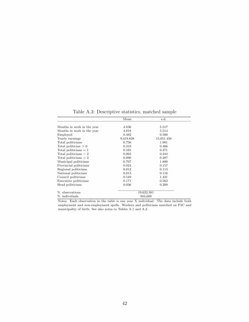
given year or not - and a total of 19.6 million year X individual observations (see Table A.3).

The individuals in our sample account for around 2 percent of the working age population

in each year.

In the sample, there are 4,638 separate F3Cs. Although, given their small number, one

might be concerned that F3Cs are a poor proxy for family connections, when interacted

with the more than 8,000 municipalities of birth, these define around 340,000 family groups.

On average, individuals in the INPS data belong to groups of around 13 individuals in the

sample. As this is a 2 percent sample of the working age population, this implies that on

average individuals belong to groups of around 650 individuals. This contrasts with best

guess estimates of between 5 and 10 individuals with the same last name and born in the

same municipality.7 This suggests that the intersection of F3C and municipality of birth

has the potential to identify families with some - although not perfect - degree of precision.

We revert to the consequences of this fuzzy matching method below, when we present our

econometric model.8

7 We derived the number of close family members (brothers, sisters, first cousins, and their children) bornin one’s municipality of birth and sharing the same F3C based on different assumptions about the numberof children across generations and geographical mobility. These simulations are available upon request.

8For each individual in the INPS sample, we can also compute the number of individuals in office carryingthe same F3C and born in the same municipality. This number is on the order of 0.76. As we have estimatedthat there are around 650 individuals with the same F3C and municipality of birth, and that between 5 and10 of them are true family members, this number will need to be rescaled by a factor of between 1/130 and1/65 in order to obtain the average number of true family members in office.

10

3 Econometric model

3.1 Specification

Having discussed the data, in this section we present the econometric model that guides our

empirical analysis. Let yiFmt denote labor outcomes in year t of worker i with F3C F born

in municipality m, and let PFmt be the number of individuals in office at time t who are

related to individual i via family ties. Ignoring other covariates, our basic model is:

yiFmt = α + βPFmt + uiFmt (3.1)

where β is the additional outcome that each politician generates among each individual

connected along family lines. The model allows different politicians to benefit different

individuals, and the same individual to benefit from multiple connections.

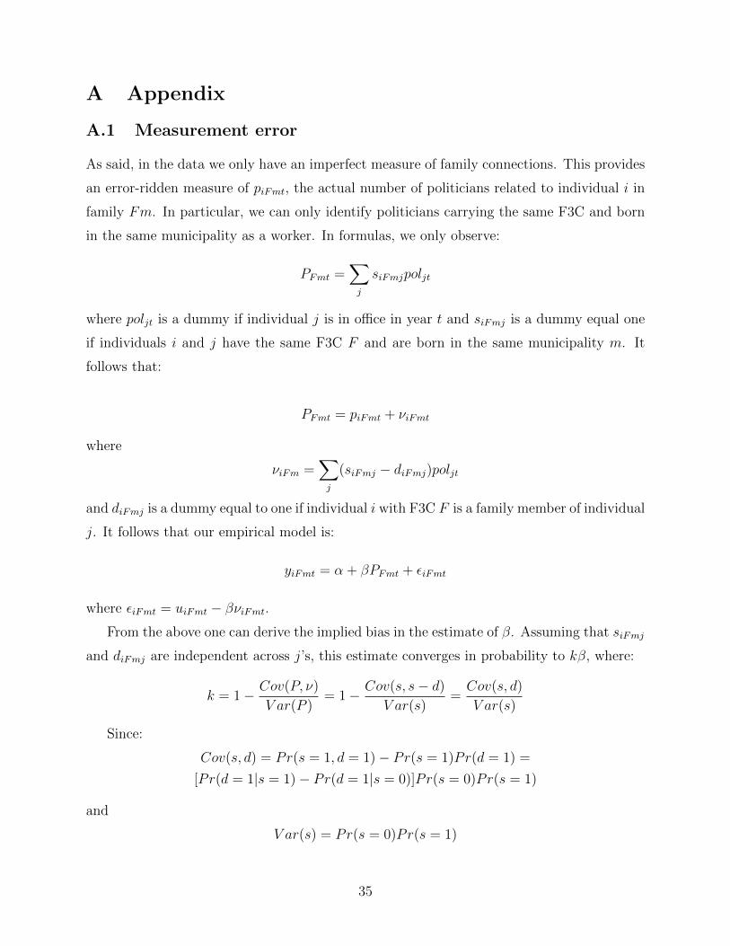
As said, one major challenge associated to the estimation of the parameter of the model

is that we have no information on actual family ties but only on whether individuals share

an F3C (and place of birth) with an individual in office. This implies that we only have

an error ridden measure of the true number of family members in office. This in turn leads

to biased estimates of the parameter β. Measurement error arises because we classify as

connected some individuals with the same F3C and municipality of birth but who are not

family members. We also fail to classify as connected individuals who are indeed linked by

family ties but who do not share the same F3C with a politician. If the control group (those

correctly classified as unrelated) is sufficiently large, this second source of measurement error

is arguably negligible.

If by NFmt we denote the number of individuals in the sample with F3C F in municipality

m at time t and by DFmt the number of individuals in the sample genuinely related to a

politician via family ties among them, one can show (see Appendix A.1) that the OLS

estimate of β converges in probability to βk, where

k = E

(DFmt

NFmt

), (3.2)

Note that k varies between 0 and 1, meaning that the OLS estimate of β will be attenuated.

The intuition for this result is straightforward: estimates that are based on F3Cs rather

than actual family ties are diluted by the fraction of those genuinely related among all those

classified as connected.

11

However, one can make some progress on the actual return to family connections based

on the distribution of the frequency of last names, NFmt, which is known. In particular, one

can allow the model parameters to vary across groups of individuals with different frequency

of last names in each municipality of birth. One implication of equation (3.1) is that these

returns will fall as NFmt increases, as measurement errors gets exacerbated.

One can also regress the outcome variable on the ratio between the number of politicians

and the frequency of individuals with the same F3C and born in the same municipality. In

formulas:

yiFmt = α + θ

(PFmt

NFmt

)+ uiFmt (3.3)

From the above, the OLS estimate of θ will converge in probability to βE(DFmt). This

is an estimate of the total return to holding office among the truly related individuals in the

sample. As the sample accounts for 2 percent of the working age population, one can simply

rescale this number by a factor of 50 to estimate the total labor market return from holding

office among the population of working age individuals.

4 Model estimates

We start by focusing on estimates of our basic model (3.1), namely the effect among those

with the same F3C and born in the same municipality. As said, these are conservative

estimates of the parameter of interest. We present a number of checks to convince a reader

that our estimates are truly causal. For most of the analysis, we exclude workers with a

frequency of the F3C in their municipality of birth in the INPS data greater than 30, the

90th percentile of the distribution. We do so to attenuate the consequences of measurement

error. Later on in the paper we also present separate regression results by classes of F3C

frequency, including for those with a frequency greater than 30. In closing we turn these

estimates into estimates of the total return to holding office on family members’ earnings

and employment outcomes based on equation (3.3).

4.1 Main estimates

In our main specification, we include in the model individual fixed effects and time effects

interacted with province (effectively, live-to-work areas) of birth dummies. Identification of

12

β is based on a differences-in-differences strategy that relies on a comparison of changes in

individuals’ labor market outcomes before and after somebody in their family assumes or

leaves political office with the same outcomes for individuals who remain (un)connected over

the same period.

Table 1 presents main estimates of model (3.1). Each panel refers to different depen-

dent variables (months of work, and earnings during the year, respectively), while separate

columns refer to different specifications. In particular, column (1) includes no controls, while

column (2) includes F3C X municipality of birth fixed effects, plus the interaction of province

of birth X year dummies in order to control for local labor market conditions. Column (3)

additionally includes age dummies plus a gender dummy. Column (4) finally includes in-

dividual fixed effects. Standard errors in these and all other regressions are clustered by

municipality of birth.

By and large, the inclusion of additional controls leads to point estimates that are in-

creasingly smaller in absolute value but consistently positive and statistically significant at

conventional levels. Focusing on the most saturated specification in column (4), this suggests

that one politician in office increases months of work per year for each individual with the

same F3C and born in the same municipality by 0.035 months (a 0.4 percent increase relative

to a baseline number of months of work of around 9.98) and 101 euros worth of earnings per

year (a 0.5 percent increase relative to baseline earnings of around 19,500 euros).

It appears that the effects are largely due to increases in months of work rather than

earnings conditional on working. Note however that earnings gains are marginally larger than

employment gains (0.5 versus 0.4 percent). This suggests that either those who benefit from

political connections enjoy wage premia, or that these individuals are selected among those

with higher earnings potential. Separate results (not reported but available upon request)

also suggest that most of the effects on months of work come from actual employment changes

rather than increases in months of work among those already in employment.

Table A.4 explores the differential effect of political connections by jobs and workers’

characteristics. We start by investigating the type of jobs accruing to politicians’ family

members, running separate regressions by occupation (blue collar, white collar and manager).

Note that different occupations correspond to alternative employment outcomes rather than

to intrinsic individual attributes. To perform this analysis, hence, for each individual in

the sample we create separate outcome variables for months of work and earnings in each

13

occupation. If an individual is not employed in a certain occupation at time t (either because

not employed at all or employed in another occupation), the outcome variable is set to zero.

The sum of the effects across occupations delivers the overall effect reported in Table 1. The

last row of Table A.4, columns (1) to (3), shows average earnings and months of work in

each occupation among all individual in our sample. An average individual in the sample,

for example, makes 4,637 euros of blue-collars’ earnings and 510 euros worth of managers’

earnings per year.

We find positive effects for each occupation type. For example, political connections are

responsible for an additional 46 euros worth of blue collar workers’ earnings and 0.029 blue

collar months of work per year. The same figures for managers are 21 euros and 0.001 months

of work. Importantly, effects are proportionally higher the higher the level of occupation.

These results suggest that jobs created by politicians are disproportionately high-paying.

This is likely to partly explain why we find effects on earnings that are proportionally higher

than for months of work (see Table 1).

We also investigate whether any heterogeneity exists by age. Using the same specification

as in column (4) of Table 1, in column (4) we interact the regressor with dummies for workers’

age groups. Estimated effects are positive for younger individuals and they tend to decline

with age. The estimated effect on earnings is negative for individuals fifty-five years of age

or older, on the order of -337 (-368 + 31) euros. Possibly this is due to earlier transitions to

retirement, or to transitions to other sectors (the public sector or even political careers) as

a result of political connections. In sum, it appears that political connections grant access

to jobs that are better than the average job, and that younger workers are those who most

benefit from these connections.

4.2 Threats to identification and additional tests

As discussed above, the identification is based on changes in labor market outcomes before

and after a family member assumes or leaves office vis-a-vis changes in labor market outcomes

among individuals in the same labor market who over the same time period remain either

consistently connected or unconnected. A concern remains that unobserved trends in family

fortunes might simultaneously lead to movements of a family member into or out of office

and an improvement or deterioration in labor market prospects of other members, hence

leading to a spurious correlation between yiFmt and PFmt, and hence a bias in the estimates

14

of β. For this purpose, we have performed a number of checks aimed at corroborating the

identification assumption.9 Some of these are reported in Table A.5, where we focus on the

most saturated specifications in column (4) of Table 1.

In column (1) we restrict to workers ever connected, i.e., with at least one family member

in office during the twenty-seven-year period. Identification is based on differential timing

of entry into or exit from office across groups. By restricting to those ever connected,

we somewhat temper the concern that those connected have different latent trends in labor

market status from those unconnected that might happen to be correlated with their families’

political fortunes. This selection criterion reduces the sample by almost 50 percent but results

are very similar to those in Table 1.

We also experimented with very flexible specifications where we interact individual fixed

effects with linear time trends or with dummies for shorter sub-periods. Once we include

the interactions of individual fixed effects with a linear time trend in column (2), results

remain virtually unchanged. In columns (3) to (5) we include respectively dummies for 8-,

4- and 2-year sub-periods interacted with individual fixed effects. Note that identification

here relies on increasingly close observations around the time of entry into or exit of a family

member from office, hence leading to less precise estimates. Point estimates fall in magnitude

compared to those in Table 1, but remain positive and statistically significant at conventional

levels.10

9 Alternatively, we could have used a RD strategy, comparing labor market outcomes of families of thosewho barely won and barely lost in close elections. Although appealing in theory, this approach is unfeasiblein this context. The major limitation is that (with the exception of some municipal elections towards theend of the period), we do not have data on candidates other than those who won the election. This problemis further compounded by the circumstance that most of the elections in Italy are held under party ratherthan individual ballot system.

10 Results (not reported) also show that our estimates are insensitive to the start years used to mark thebeginning of each 8-year, 4-year and 2-year time interval. We have also performed a number of additionalrobustness checks (not reported but available upon request). First, we show that coefficients remain statisti-cally significant at conventional levels if we cluster standard errors at the level of province as opposed to cityof birth. We have also estimated regression coefficients from a model where we include (8,110) municipalityof birth X (27) year fixed effects. This allows us to control for the state of the labor market at a verylocalized level. By including municipality (as opposed to province) of birth X year fixed effects, though,our control group includes individuals with a different F3C in any given municipality (as opposed to anygiven province). This exacerbates type-1 error (see equation (A.1) in Appendix A.1). Indeed, the inclusionof municipality of birth X year fixed effects reduces the point estimates sensibly (a five-fold reduction forearnings and thirty-fold reduction for months of work) although the effects remain positive and typicallysignificant.

15

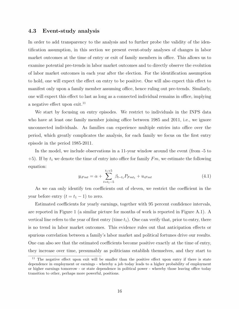
4.3 Event-study analysis

In order to add transparency to the analysis and to further probe the validity of the iden-

tification assumption, in this section we present event-study analyses of changes in labor

market outcomes at the time of entry or exit of family members in office. This allows us to

examine potential pre-trends in labor market outcomes and to directly observe the evolution

of labor market outcomes in each year after the election. For the identification assumption

to hold, one will expect the effect on entry to be positive. One will also expect this effect to

manifest only upon a family member assuming office, hence ruling out pre-trends. Similarly,

one will expect this effect to last as long as a connected individual remains in office, implying

a negative effect upon exit.11

We start by focusing on entry episodes. We restrict to individuals in the INPS data

who have at least one family member joining office between 1985 and 2011, i.e., we ignore

unconnected individuals. As families can experience multiple entries into office over the

period, which greatly complicates the analysis, for each family we focus on the first entry

episode in the period 1985-2011.

In the model, we include observations in a 11-year window around the event (from -5 to

+5). If by t1 we denote the time of entry into office for family Fm, we estimate the following

equation:

yiFmt = α +

t1+5∑t=t1−5

βt−t1PFmt1 + uiFmt (4.1)

As we can only identify ten coefficients out of eleven, we restrict the coefficient in the

year before entry (t = t1 − 1) to zero.

Estimated coefficients for yearly earnings, together with 95 percent confidence intervals,

are reported in Figure 1 (a similar picture for months of work is reported in Figure A.1). A

vertical line refers to the year of first entry (time t1). One can verify that, prior to entry, there

is no trend in labor market outcomes. This evidence rules out that anticipation effects or

spurious correlation between a family’s labor market and political fortunes drive our results.

One can also see that the estimated coefficients become positive exactly at the time of entry,

they increase over time, presumably as politicians establish themselves, and they start to

11 The negative effect upon exit will be smaller than the positive effect upon entry if there is statedependence in employment or earnings - whereby a job today leads to a higher probability of employmentor higher earnings tomorrow - or state dependence in political power - whereby those leaving office todaytransition to other, perhaps more powerful, positions.

16

decline precisely after four years, i.e., towards the end of an electoral term. In Figure 2 (and

Figure A.2) we examine politicians’ exit from office and, similarly to entries, we run the

following regression:

yiFmt = α +

tN+5∑t=tN−5

βt−tNPFmtN + uiFmt, (4.2)

where tN denotes the time of last exit from office for family Fm. Again, we focus on the

last exit episode in order to limit the possibility that subsequent exits might confound our

estimates and we restrict the coefficient in the year after exit tN + 1 to zero.

Differently from what was found for entries, there is evidence of a deterioration in out-

comes predating the time of exit, which continues after the time of exit itself. We take

this evidence to suggests that exits are somewhat anticipated, which is reasonable given the

normal length of a term and the fact that information on those running for the next election

is somewhat known in advance.12

In sum, this and the preceding subsections have provided an array of corroborating

evidence in favor of our identification assumption. We have shown that results remain

essentially unchanged if we only restrict to individuals who at one point over the period of

analysis are connected and if we allow for rather flexible time trends in individuals’ latent

labor market outcomes. Perhaps more importantly, we have used an event-study analysis

to show that pre-entry trends in outcomes are de facto the same across treatment and

control groups and effects manifest precisely upon entry and last as long as individuals in

the family stay in office. These pieces of evidence speak strongly in favor of our identification

assumption.

12 Entry and exit episodes might not be good predictors of the actual number of family members in officein nearby years. This happens, for example, if a politician’s entry into office is systematically associated toan exit in the same family, implying that there is no effect on the total stock of individuals in office in thefamily when an entry or an exit occur. In order to address this concern, in Figure A.3, we report results fromregressions similar to (4.1) and (4.2), where now the dependent variable is the number of family membersin office at time t (effectively a first stage equation). One can see that the first entry episode is a strongpredictor of the total number of family members in office, with a coefficient close to one. One can also seethat the number of politicians in office declines precisely five years after entry, consistent with political termsbeing typically four years. Similarly, we find evidence of the last exit episode being a clear and significantpredictor of the number of politicians in the family in office in surrounding years (see Figure A.4).

17

5 Implied returns to nepotistic hiring

Having ascertained that our estimates capture the causal effect of being born in the same mu-

nicipality and carrying the same F3C as one individual in office, we now present calculations

on the overall return to office in terms of family private sector earnings.

As said, one way of interpreting the estimates in the previous section is that these are

error-ridden estimates of the true effect of family connections. This error is likely to be larger

the larger the size of the group. Column (1) of Table 2 reports a pooled estimate where -

consistent with equation (3.3) - we impose that the effect varies in an inverse linear fashion

with the frequency of the group NFmt. In order to measure the size of the groups, we use the

median size across the twenty-seven years of analysis. The estimated coefficient provides a

measure of the total return to holding office in terms of labor market earnings in the 2/100

INPS sample. The point estimate for earnings is 180 euros, implying that each politician is

able to extract around 9,000 euros of private labor market earnings for his family for each

year in office. As for employment, the same figure is about 4 months of work in a year.

Rather than imposing that the coefficient in (3.3) varies parametrically with NFmt, one

can also estimate separate parameters by the (sample) frequency of the distribution of F3Cs

in one’s municipality of birth. As said, one will expect larger estimates for smaller groups,

as measurement error is less of an issue in this case. In columns (2) to (5) we present

separate regressions for frequencies 1, 2-5, 6-30 and more than 30. Consistent with our

measurement error model, the effects decline monotonically with the frequency of the F3C.

The average return among individuals in groups of sample size 1 is around 108 euros, implying

an estimated total effect in the population of around 2,160 euros (108 X 50). Effect among

individuals in groups with a sample size of between 2-5 (geometric mean of the distribution

of frequencies 0.37) is 71 euros, implying a total effect of around 9,500 euros (71 X 50 / 0.37).

Finally, in the group of frequency 6-30 (geometric mean 0.10) the effect is 31 euros, implying

an overall effect of around 15,500 euros (31 X 50 / 0.10). Similar patterns emerge when

looking at months of work in the bottom panel of Table 2. Overall, estimates of the total

return appear to increase with the number of individuals in the group, which is potentially

due to a greater number of family members living in the same municipality for larger groups

(i.e, a lager DFmt).

The above estimates refer to the labor market returns to being politically connected.

Based on these estimates, one can also attempt to derive estimates of the overall number

18

of private sector jobs and earnings that politicians are able to generate among their family

members, and the overall effect of nepotism. We have estimated an average return to holding

office of about 4 months of work per year. As there are approximately 137,000 individuals

in office per year, this implies that at least 45,000 (137,000 X 4 / 12) jobs per year can be

ascribed to political nepotism along family lines. This is around 0.4 percent of private sector

employment in INPS, i.e., 4 workers out of 1,000.

6 Nepotistic hiring and corruption

In the previous section we have argued that there are sizeable effects of having a family

member in office on private labor market outcomes. Clearly, per se this is not evidence of

corruption. In this section hence we bring ammunition to our claim that this phenomenon is

based on a quid-pro-quo exchange between politicians and firms. In the following we present

an array of evidence consistent with our interpretation.

6.1 Rents in office

We start by showing that the incidence of nepotistic hiring is positively associated to politi-

cians’ clout and to the resources available to the office where they serve. This is consistent

with the view that this is a technology of rent appropriation on the part of politicians.

We present regression estimates in Table 3 where we revert to the main specification in

Table 1, column (4) (i.e, without adjustment for group size). Columns (1) to (3) report

respectively separate estimates on the number of family members in office in council and

executive positions, on the number of politicians by number of consecutive terms in the

same office (1 term, 2 terms or more) (including the number of individuals in office in 1985

to control for the left censored nature of the data) and on the number of politicians at

different levels of government (municipal, provincial, regional and national).

The table illustrates that more powerful politicians tend to generate higher labor market

returns among their family members. Column (1) shows that those in the executive positions

(whether commissioners in municipal, provincial or regional governments, or ministers in the

central government, or heads of the executive) generate returns that are around 50 percent

higher than those in council positions.

Column (2) shows that yearly returns among those in office for two terms or more are

around three times as much as those found among those in office for only one term. This is

19

evidence of the returns increasing with tenure, although it is possible that those with longer

tenure are more powerful or able politicians, including those more able to appropriate rents

for themselves and their families.

A similar positive gradient is found among politicians at higher levels of government (e.g.,

regional) compared to those at lower levels (e.g., municipal), at least as long as earnings are

concerned, although results other than for municipal politicians are typically imprecise, which

is unsurprising given that most politicians serve at the local level.

We also present results based on the amount of resources available to politicians. In order

to perform this exercise, we follow a two-step procedure. We start by estimating a separate

parameter βm as in equation (3.1) for each municipality. As we exploit cross-municipality

variation in local budget, we restrict to the effect of municipal politicians only. However, we

have shown above that most of the effects of nepotism are ascribable to municipal politicians.

In a second step we regress these municipality-specific measures of nepotism on municipality-

level variables with weights equal to the reciprocal of the square of the standard error of each

coefficient, in the spirit of a minimum distance estimator.13

In order to measure the resources available to those in office we use public expenditure

per politician (in logs). We restrict to a measure of discretionary expenditure, defined as

total expenditure net of debt service and personnel, as this is easier and hence more likely to

be used to foster nepotistic practices. We have also experimented with other measures of the

local budget (total expenditure and total revenues per politicians). Results (not reported)

are qualitatively similar but less precise.

Column (1) of Table 4 presents these estimates with no additional controls. These and all

other regressions are restricted to the municipalities with non-missing values of all included

regressors. As, clearly, the amount of spending is not randomly allocated across municipal-

ities and some determinants of spending might be correlated with the amount of nepotism,

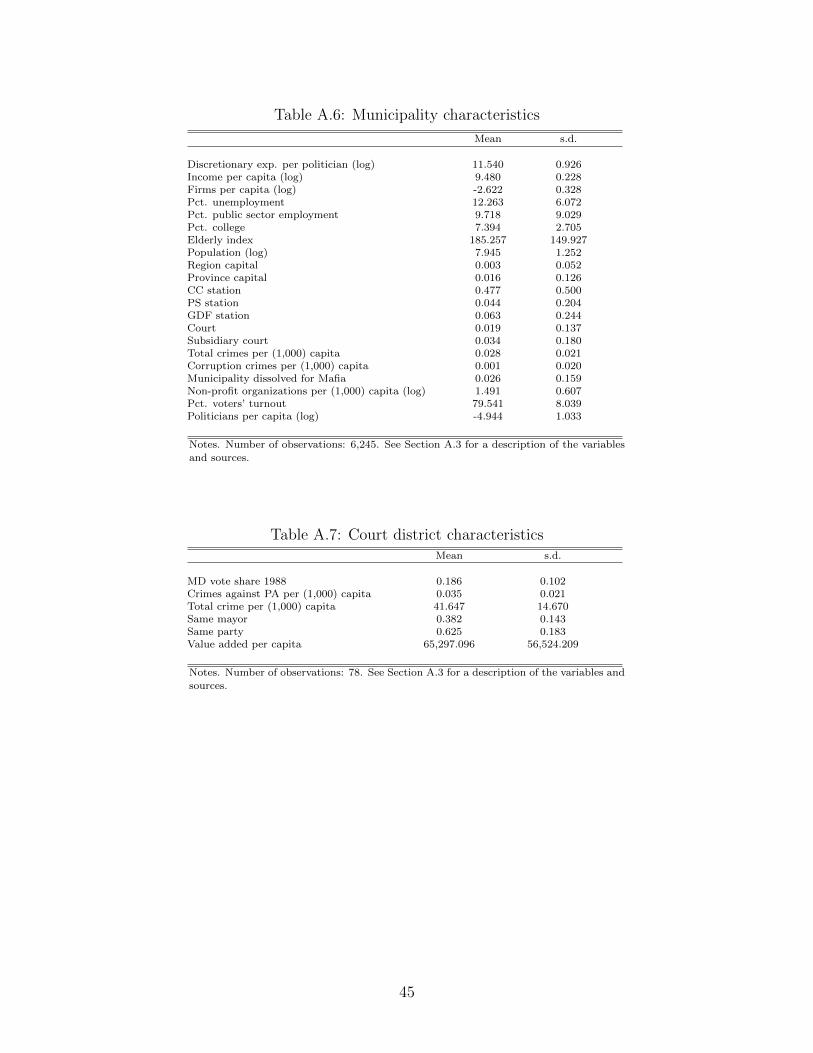
we additionally include in the model a large number of observable municipality-level charac-

teristics (see Appendix A.3 and Table A.6). If anything, the inclusion of municipality-level

controls leads to estimates, in column (2), that are larger than estimates with no controls in

column (1). Finally, we include in the model province fixed effects. Identification is across

municipalities with the same characteristics within each of the 103 provinces. Once more,

13 For about 2,000 municipalities, not enough observations are available to identify a municipality-specificcoefficient. As a robustness check we have run the pooled regression in Table 1, column (4) on this restrictedsample of residual 6,245 municipalities. Results are remarkably similar to those obtained for the entiresample.

20

point estimates increase when we include these additional controls. It appears that a 10

percent increase in resources per politician leads to a roughly 30 percent increase compared

to the average estimates in Table 1 (0.1 X 331 / 101 = 0.32 for yearly earnings, and 0.1 X

0.136 / 0.035 = 0.38 for months of work).14

In sum, there is clear evidence of the effects of connections displaying a positive gradient

in politicians’ clout and in the resources under their control, which lends support to our

interpretation of the coefficients as measuring rent extraction on the part of politicians.

6.2 Public influence over firms

Although we have presented evidence that nepotism correlates positively with the power

associated to office, this clearly does not rule out interpretations alternative to corruption.

Ideally, one would like to simultaneously show that firms derive a private utility from hiring

or promoting politicians’ relatives. As this cannot be done with our data, as the identity of

firms is concealed, we address this issue by showing that effects are larger in sectors that are

more dependent on the public administration. If nepotistic hiring is driven by considerations

other than political returns for firms, one will not expect such a systematic pattern.

To perform this exercise, we use the Public Sector Dependence Score by Pellegrino and

Zingales (2014). This index is based on the number of news articles on regulation policy

and government aid and contracts as a percentage of the total number of news articles

per sector (twenty-five sectors overall) between 2000 and 2012. The index varies between

around 1.5 percent in Basic Metals and Fabricated Metal Products to over 9 percent in

Agriculture, Hunting, Forestry and Fishing. While this index is clearly a coarse measure

of public influence, it has the advantage of capturing the two main channels through which

politics might interfere with firms’ activities, i.e., regulation and public transfers.

As in the previous sub-section, we use a minimum distance estimator. First, we obtain

separate regressions for each of the fifty ATECO-81 sectors, which is the industrial classifi-

cation used in the INPS data.We then regress these coefficients on Pellegrino and Zingales’

14 Note that, for politicians we use the characteristics of the municipality of birth (as opposed to the oneof election). Not only does this greatly simplify the empirical analysis, but it also has the advantage ofcircumventing the potential non-random allocation of those in office. The concern here is that those withstronger propensity to engage in nepotistic practices might seek office in areas where the return to this activityis higher or where discretionary spending is higher. In this sense, our estimates can be interpreted as intent-to-treat estimates of the effect of local resources on the incidence of nepotism. Separate regressions showthat discretionary expenditure in the municipality of birth is a strong predictor of discretionary expenditurein the municipality of election. This is consistent with the fact that around 50 percent of local politiciansserve in their city of birth.

21

Public Sector Dependence Score. We cluster standard errors at the level of variation of

Pellegrino and Zingales’ sectors. Point estimates reported in Table 5 are systematically

positive, although statistically significant at conventional levels only for yearly earnings. A

back-of-the-envelope calculation suggests that moving from the least regulated sector to the

most regulated one (7.5 percentage points) leads to an increase in the monetary returns to

political connections of around 8 percent (7.5 X 1.106 / 101 = 0.08).15

In sum, we find evidence of the effects being larger in more regulated sectors, which

is consistent with the view that the phenomenon we uncover is driven by a quid-pro-quo

exchange between firms and politicians.

7 Nepotism vis-a-vis other modes of corruption

The obvious question that remains is why, in an attempt to extract rents that accrue to

their office, politicians engage in these practices as opposed to simple grafting or eliciting

monetary bribes from firms.

In this section we argue that this practice is a substitute, possibly an inferior one, for

other, more visible and easier to detect, forms of corruption. Although the returns to nepo-

tistic hiring are presumably lower, as jobs are not necessarily fungible for money, nepotistic

practices are also less likely to be discovered and lead to prosecution, and hence their cost

is also presumably lower.

In order to bring suggestive evidence in favor of this claim, we exploit a major natural

experiment induced by “Mani Pulite” (or “Clean Hands”), an aggressive judicial prosecution

campaign against cases of corruption linked to payment of bribes to the then majority parties

(Christian Democrats and Socialists) that swept Italy starting in 1992 (see The New York

Times 1993). Importantly, the focus of the investigations was on payment and receipt of

monetary bribes, both because these were apparently very widespread (hence the name

of “Tangentopoli”, or “Bribopolis”, coined at the time), and, more importantly, as illicit

transfers and funds represented the primary source of evidence brought by prosecutors in

most of these cases.

15 A final concern remains that some firms in the INPS data, even if belonging to the private sector, arepublicly owned. Most of these firms are owned by municipalities, operating as providers in the utilities andtransport sectors. Other firms might be in the banking sector. Figure A.5 and A.6 report the proportionalincrease in yearly earnings and months of employment due to nepotism, by one-digit sector. There is noevidence that these effects are systematically larger in these sectors.

22

Clean Hands exploded after a period when the judiciary had been dormant in the face

of rampant corruption. A widespread view (see, e.g., Il Foglio 2016) is that the campaign

was initiated and carried forward by prosecutors with links to Magistratura Democratica (in

brief MD), the left-wing faction of the Associazione Nazionale Magistrati (in brief ANM), the

independent official body that represents the interests of judges and prosecutors. MD had

historical ties to the minority Communist Party, traditionally in opposition to the majority

coealition parties (Christian Democrats and Socialists).16

We exploit the pre-1992 differences in the fraction of judges and prosecutors affiliated with

MD across the twenty-six Italian judicial districts to predict how aggressive the Clean Hands

campaign was across areas. Importantly, as in Italy judges and prosecutors are appointed

to office largely based on seniority, this should guarantee that this variation is exogenous to

other major determinants of corruption and nepotistic hiring. One will expect the judiciary

to more aggressively prosecute cases of payment of monetary bribes in areas where MD was

stronger. If nepotistic hiring is a substitute for payment of monetary bribes, one will also

expect a rise in nepotistic hiring where MD was stronger.

Table 6 reports regression results where each dependent variable is regressed on district

fixed effects, time (1985-1991, 1992-2000, 2001-2011) fixed effects and the interaction of the

district-level share of pre-Clean Hands (1988) votes for MD in the election for the Comitato

Direttivo Centrale of the ANM (see www.associazionemagistrati.it).17 18

Column (1) of Table 6 reports results where the dependent variable is the (log) number of

per capita crimes against the public administration for which prosecution started in each of

the twenty-six districts, averaged over three time sub-periods. These crimes include wrong-

doing on the part of both public officials and private agents, and also include payment and

receipt of monetary bribes, as well as grafting. For ease of interpretation, we normalize the

MD vote share by the standard deviation across court districts. Consistent with increased

enforcement, the data show that the number of prosecuted cases increased less in courts with

16 Out of the eight leading members of the Clean Hands team in the district attorney office of Milan, wherethe campaign started, six (Davigo, Colombo, Boccassini, Borrelli, D’Ambrosio and Greco) were members ofMD at the time of the investigations.

17 Exhaustive data on individuals’ affiliation to the different factions of the ANM are not publicly available.18 Not surprisingly, in the 1991 elections the share of MD in the district of Milan was the third highest

in the country (35 percent, compared to a 20 percent national average). Soon after Milan, the campaignspread to other districts, especially those with a higher fraction of votes for MD. Among these: Brescia (31percent), Genoa (36 percent), Turin (27 percent) and Florence (28 percent), but also Rome (19 percent) andNaples (20 percent).

23

a higher share of votes for MD.19 Differences in reported crimes between courts one standard

deviation apart in terms of MD vote shares fell by around 13 percent in the aftermath of

Clean Hands, and they remained persistently lower in the following decade (with a difference

of around 21 percent). Results (not reported) also hold but are marginally less significant

if we include in the model the interaction between macro area dummies (North, Centre and

South) and sub-period dummies.

As a concern remains that trends across areas with different vote shares for MD are

correlated with trends in corruption for reasons other than stricter enforcement - be it because

of omitted variables or other mediating mechanisms - in columns (2) to (5) of Table 6

we present similar regressions with different dependent variables (see Appendix A.3 and

Table A.7 for a description of these variables). In column (2) we report a regression where

the dependent variable is total reported crimes per capita (in logs). Effects are small and

statistically undistinguishable from zero. As the Clean Hands campaign might have affected

the selection of politicians or local economic activity, and this might have an independent

effect on the spread of corruption, in columns (3) to (5) we report regressions where the

dependent variable is, in turn, the fraction of incumbent mayors, the fraction of mayors who

are from the incumbent party, and the (log) value added per capita. None of these variables

follow trends that are correlated with the pre-campaign share of MD votes in that area. In

sum, these regressions are suggestive of the treatment not capturing or producing effects

along other relevant confounding paths.

In columns (6) and (7) we finally report regressions where the dependent variable is a

measure of nepotistic hiring, in terms of earnings and months of work respectively. Once

more, we have estimated equation (3.1) separately across the twenty-six district courts and

the three sub-periods, and we use a minimum distance estimator. The coefficient on the

interaction terms are positive and statistically significant. Magnitudes are also high: a one

standard deviation increase in the MD vote share leads to a rise in the incidence of nepotistic

hiring of between 65 and 82 percent (66 additional euros in the 1990s and 83 euros in the

2000s, relative to a baseline effect of 101 euros in Table 1). Similar results emerge for

the number of months of work, although estimates are not statistically significant for the

sub-period 2001-2011.

19 Clearly, by prosecuting cases more aggressively these courts might have also detected more cases,especially in the early period. This would have led to a rise in the observed crime rate. In this case, theestimate in column (1) is an upper bound for the effect of increased deterrence on corruption.

24

In sum, this section provides suggestive evidence in favor of a rationale for nepotistic hir-

ing: when monetary bribing and grafting become more costly, both private firms and officials

might prefer harder-to-detect technologies of rent appropriation. This evidence suggests that

the availability of alternative forms of exchange between firms and politicians may reduce

the effectiveness of monitoring as a tool to contrast corruption (Olken and Pande 2012).

8 Discussion and conclusions

In this paper we estimate the effect of family connections to public officials on private labor

market outcomes in Italy. Although there is plenty of anecdotal evidence on practices of

favoritism in hiring and promotion of public officials’ relatives, credible evidence is by and

large missing, and it is difficult to establish if these practices are ascribable to a quid-pro-quo

exchange between politicians and firms.

We estimate sizeable returns to holding political office, on the order of 9,000 euros and

4 months of work per year. Back-of-the-envelope calculations suggest that jobs acquired

through nepotism account for at least 0.4 percent of private sector employment in Italy.

Our estimates clearly only refer to nepotism along family lines and exclude other forms of

interference with the hiring decisions of private firms on the part of public officials through

favoring of “friends” or other associates, including political associates. They also only refer

to family members born in the same municipality and with the same F3C. In this sense,

these are likely to provide a lower bound for the true effect of nepotistic hiring in the private

sector labor market as they exclude relatives born elsewhere or those with a different last

name (and hence F3C), including affinal relatives.

We speculate that nepotism is the result of an exchange between firms and politicians.

We take the evidence in the paper, that the estimated effect increases with a politician’s

clout and with the resources accruing to the administration where he serves, to indicate that

nepotism is indeed a technology of rent appropriation that helps politicians monetize over

their position of power.

However, the question remains as to why politicians and firms resort to nepotistic hiring

in exchange for what we claim as being political favors. We speculate and present suggestive

evidence in favor of the hypothesis that nepotism is a - potentially inferior - substitute for

grafting and monetary bribes: when these are costly, due to high rates of detection, both

firms and officials will shift towards harder-to-detect technologies of rent appropriation.

25

References

[1] Acemoglu D., S. Johnson, A. Kermani , J. Kwak J. and T. Mitton, 2016. “The Value of

Connections in Turbulent Times: Evidence from the United States.” Journal of Financial

Economics, 121, 368-391.

[2] Alesina A. and P. Giuliano, 2014. “Family Ties.” In Handbook of Economic Growth,

Aghion P. and S. Durlauf (eds.), North Holland, vol. 2a, 177-215.

[3] Banerjee A., R. Hanna and S. Mullainathan, 2012. “Corruption.” In The Handbook of

Organizational Economics, Gibbons R. and J. Roberts (eds.), Princeton University Press,

1109-1147.

[4] Banfield E. C., 1958. The Moral Basis of a Backward Society, Free Press.

[5] Bertrand M., F. Kramarz, A. Schoar and D. Thesmar, 2007. “Politically Connected CEOs

and Economics Outcomes: Evidence from France.” Mimeo, MIT.

[6] Bertrand M. and A. Schoar, 2006. “The Role of Family in Family Firms.” Journal of

Economic Perspectives, 20, 73-96.

[7] Black S. E. and P. J. Devereux, 2011. “Recent Developments in Intergenerational Mobil-

ity.” In Handbook of Labor Economics, Ashenfelter O. and D. Card (eds.), Elsevier, vol.

4b, 1487-1541.

[8] Brollo F., T. Nannicini, R. Perotti and G. Tabellini, 2013. “The Political Resource Curse.”

American Economic Review, 103, 1759-1796.

[9] Caffarelli E. and C. Marcato, 2008. I Cognomi d’Italia: Dizionario Storico ed Etimologico,

UTET.

[10] Cingano F. and P. Pinotti, 2013. “Politicians at Work. The Private Returns and Social

Costs of Political Connections.” Journal of the European Economic Association, 11, 433-

465.

[11] Clark G. and N. Cummins, 2014. “Intergenerational Wealth Mobility in England, 1858-

2012: Surnames and Social Mobility.” Economic Journal, 125, 61-85.

26

[12] Dal Bo E., P. Dal Bo and R. Di Tella, 2006. “‘Plata o Plomo?’: Bribe and Punishment

in a Theory of Political Influence.” The American Political Science Review, 100, 41-53.

[13] Dal Bo E., P. Dal Bo and J. Snyder, 2009. “Political Dynasties.” Review of Economic

Studies, 76, 115-142.

[14] Durante R., G. Labartino and R. Perotti, 2011. “Academic Dynasties: Decentralization

and Familism in the Italian Academia.” NBER WP 17572.

[15] Fafchamps M. and J. Labonne, 2016. “Do Politicians’ Relatives Get Better Jobs? Evi-

dence from Municipal Elections in the Philippines.” Mimeo, Stanford University.

[16] Ferraz C. and F. Finan, 2008. “Exposing Corrupt Politicians: The Effect of Brazil’s

Publicly Released Audits on Electoral Outcomes.” Quarterly Journal of Economics, 123,

703-745.

[17] Ferraz C. and F. Finan, 2011. “Motivating Politicians: The Impacts of Monetary In-

centives on Quality and Performance.” NBER WP 14906.

[18] Financial Times, 2015. “JPMorgan Told to Provide Communications with Top Chinese

Official.” May 28, 2015.

[19] Fisman R., 2001. “Estimating the Value of Political Connections.” American Economic

Review, 91, 1095-1102.

[20] Fisman, R., N. A. Harmon, E. Kamenica and I. Munk, 2015. “Labor Supply of Politi-

cians.” Journal of the European Economic Association, 91, 871-905.

[21] Fisman R., R. Schulz and V. Vig, 2014. “The Private Returns to Public Office.” Journal

of Political Economy, 122, 806-862.

[22] Folke O., T. Persson and J. Rickne, 2017. “Dynastic Political Rents? Economic Benefits

to Relatives of Top Politicians.” Economic Journal, 127, 495-517.

[23] Gagliarducci S. and T. Nannicini, 2013. “Do Better Paid Politicians Perform Better?

Disentangling Incentives from Selection.” Journal of the European Economic Association,

11, 369-398.

27

[24] Kramarz F. and O. N. Skans, 2014. “When Strong Ties are Strong: Networks and Youth

Labor Market Entry.” Review of Economic Studies, 81, 1164-1200.

[25] Il Foglio 2016. “Compagno Magistrato.” April 17, 2016.

[26] Istat, 2010. Forze di Lavoro: Media 2008, Rome.

[27] Merlo A., V. Galasso, M. Landi and A. Mattozzi, 2010. “The Labor Market of Italian

Politicians.” In The Ruling Class: Management and Politics in Modern Italy, Boeri T.,

Merlo A. and A. Prat (eds.), Oxford University Press.

[28] Olken B., 2007. “Monitoring Corruption: Evidence from a Field Experiment in Indone-

sia.” Journal of Political Economy, 115, 200-249.

[29] Olken B. and R. Pande, 2012. “Corruption in Developing Countries.” Annual Review

of Economics, 4, 479-505.

[30] Pellegrino B. and L. Zingales, 2014. “Diagnosing the Italian Disease.” Mimeo, Chicago

University.

[31] Putnam R. D., R. Leonardi and R. Y. Nanetti, 1993. Making Democracy Work: Civic

Traditions in Modern Italy, Princeton University Press.

[32] The New York Times, 1993. “Broad Bribery Investigation Is Ensnaring the Elite of

Italy.” March 3, 1993.

[33] Transparency International, 2014. Corruption Perception Index 2014.

[34] World Bank 2014. Doing Business, available at http://goo.gl/uVno.

28

Table 1: Main estimates(1) (2) (3) (4)

Dep. variable: Yearly earnings

Politicians 442.915*** 202.799*** 104.335*** 101.136***(62.713) (17.356) (12.276) (13.783)

Dep. variable: Months of work in the year

Politicians 0.112*** 0.117*** 0.051*** 0.035***(0.017) (0.008) (0.005) (0.004)

Munic. birth X F3C FE Yes Yes YesProv. birth X year FE Yes Yes YesIndiv. controls Yes YesIndiv. FE Yes

Notes. Columns (1) to (4) of the table report the coefficients on the number of individuals in office (inany level of government and in any office) with the same F3C and municipality of birth (equation (3.1)).

Individual controls include age-group dummies (in ten year bands) and a female dummy. Standard

errors clustered by municipality of birth in round brackets. Sample is restricted to observations withat most 30 individuals with the same municipality of birth and F3C in the INPS sample. Number of

observations 17,683,130. ***, **, *: denote significant at 1, 5 and 10 percent level, respectively.

29

Table 2: Heterogeneous effects by F3C frequency

(1) (2) (3) (4) (5)Rescaled by Frequencyfrequency 1 2-5 6-30 > 30

Dep. variable: Yearly earnings

Politicians per capita 180.019***(29.533)

Politicians 107.974*** 71.427*** 31.849** -9.520(36.733) (18.381) (14.854) (11.068)

Dep. variable: Months of work in the year

Politicians per capita 0.069***(0.011)

Politicians 0.041*** 0.029*** 0.008* 0.000(0.014) (0.007) (0.005) (0.003)

Notes. Column (1) reports estimates of equation (3.3). Columns (2) to (5) report regressions similar to those in column (4) of

Table 1 separately by sample frequency of F3C in each municipality. Number of observations: 19,622,381; 5,608,780; 7,238,359;4,835,991; 1,939,251 respectively in columns (1) to (5). See also notes to Table 1.

30

Table 3: Heterogeneous effects by politicians’ characteristics

(1) (2) (3)By level of office By tenure By level of government

Dep. variable: Yearly earnings

Council 87.201***(13.308)

Head + Executive 140.822***(27.135)

1 Term 99.617***(12.868)

2 Terms 162.069***(24.833)

> 2 Terms 334.900***(49.211)

Municipal 104.263***(13.845)

Provincial 11.288(53.370)

Regional 177.915*(105.872)

National 19.164(118.820)

Dep. variable: Months of work in the year

Council 0.031***(0.005)

Head + Executive 0.047***(0.008)

1 Term 0.037***(0.004)

2 Terms 0.053***(0.008)

> 2 Terms 0.084***(0.016)

Municipal 0.035***(0.004)

Provincial 0.034**(0.017)

Regional -0.004(0.040)

National 0.060(0.041)

Notes. The table reports regressions similar to those in column (4) of Table 1 where the effects are

allowed to vary by politicians’ characteristics. Regressions in column (2) additionally include thenumber of left censored observations (individuals in office in 1985) by F3C and municipality. See also

notes to Table 1.

31

Table 4: Discretionary spending and nepotism

(1) (2) (3) (4) (5) (6)

Dep. variable: Nepotism - Nepotism - Nepotism - Nepotism - Nepotism - Nepotism -yearly yearly yearly months months months

earnings earnings earnings of work of work of work

Spending per politician (log) -10.615 236.025*** 330.792*** -0.004 0.082*** 0.136***(22.830) (70.124) (81.429) (0.010) (0.032) (0.036)

Additional controls No Yes Yes No Yes YesProvince FE No No Yes No No Yes

Notes. The table reports minimum distance estimates of the effect of log discretionary spending per politician on the extent of

nepotism by municipality. Regressions refer to municipal politicians only. Dependent variables are the coefficients on nepotismseparately estimated by municipality (columns 1-3 and 4-6, respectively for earnings and months of work) as in column (4) of

Table 1. Method of estimation: GLS, with weights equal to the square of the reciprocal of the standard error associated to each

coefficient. In all estimates we control for the log total number of local politicians, and log local population. Additional controlsare log income per capita, log number of firms per capita, fraction of workers in the public sector and local unemployment

rate, fraction of population with a college degree, fraction of the population that is past working age, dummies for whether a

municipality is a region or province capital, dummies for whether the municipality has a police station (separately for the threepolice forces in Italy, Carabinieri, State Police and Guardia di Finanza) and for whether this is a site of a judicial court. In

order to proxy for different level of social capital across areas we include a measure of turnout in local elections, log number of

non-profit associations per capita, and a dummy for whether the municipal administration was ever dissolved for mafia,whichproxies for the presence of organized crime. Precise sources and definitions together with descriptive statistics are presented in

Appendix A.3 and Table A.6. See also text for details. Robust standard errors in brackets. Number of observations 6,245. ***,

**, *: denote significant at 1, 5 and 10 percent level, respectively.

Table 5: Government dependence and nepotism

(1) (2)

Dep. variable: Nepotism - Nepotism -yearly months

earnings of work

Pellegrino & Zingales’ Government dependence index 1.106*** 0.096(0.382) (0.117)

Notes. The table reports minimum distance estimates of the effect of government dependence by

industrial sector on the extent of nepotistic hiring. Method of estimation: GLS, with weights equal tothe square of the reciprocal of the standard error associated to each coefficient. Dependent variablesare the coefficients on nepotism separately estimated by ATECO-81 2-digit sector (columns 1 and 2,

respectively for earnings and months of work) as in column (4) of Table 1. See also text for details.Standard errors clustered by twenty-five industrial sectors in Pellegrino and Zingales (2014) in brackets.

Number of observations 50. ***, **, *: denote significant at 1, 5 and 10 percent level, respectively.

32

Table 6: Nepotistic hiring vis a vis other modes of corruption

(1) (2) (3) (4) (5) (6) (7)Dep. variable: Crimes Same Same Value added Total Nepotism - Nepotism -

against PA mayor party per capita crimes yearly months(log) (log) (log) earnings of work

MD X (1992-2000) -0.126* 0.052 0.036 0.005 -0.014 65.947** 0.035**(0.071) (0.037) (0.035) (0.030) (0.056) (28.210) (0.016)

MD X (2001-2011) -0.214*** 0.027 0.041 0.084*** -0.043 83.114*** 0.023(0.071) (0.037) (0.035) (0.030) (0.056) (30.524) (0.016)

Notes. The table reports minimum distance estimates of the effect of the 1988 elections MD (Magistratura Democratica)vote share by district court on different outcomes, interacted with dummies for time sub-periods (1992-2000, 2001-2011). All

regressions include 26 district court dummies. Dependent variables are: log crimes against the public administration per capita(column 1), population weighted fraction of municipalities where mayor is an incumbent or from the incumbent mayor’s party

(columns 2 and 3), log value added per capita (column 4), log total crimes per capita (column 5), coefficients on nepotism

separately estimated by district court and sub-period (columns 6 and 7, respectively for yearly earnings and months of work) asin column (4) of Table 1. Method of estimation: GLS, with weights equal to cell population (columns 1 to 5) or the square of

the reciprocal of the standard error associated to each coefficient (columns 6 and 7). See also text for details. Robust standard

errors in brackets. Number of observations 78. ***, **, *: denote significant at 1, 5 and 10 percent level, respectively.

33

Figure 1: Event-study analysis: Yearly earnings - entry

02

00

40

0

−5 −4 −3 −2 −1 0 1 2 3 4 5

Years to/from event

Notes. The figure displays estimated yearly earnings at different lags andleads since the time of first entry (denoted by a vertical line). All coeffi-cients expressed relative to effect in year before entry. 95 percent confidenceintervals reported. See also text for details.

Figure 2: Event-study analysis: Yearly earnings - exit

−2

00

02

00

40

0

−5 −4 −3 −2 −1 0 1 2 3 4 5

Years to/from event

Notes. The figure displays estimated yearly earnings at different lags andleads since the time of last exit (denoted by a vertical line). All coefficientsexpressed relative to effect in year after exit. 95 percent confidence intervalsreported. See also text for details.

34

A Appendix

A.1 Measurement error

As said, in the data we only have an imperfect measure of family connections. This provides

an error-ridden measure of piFmt, the actual number of politicians related to individual i in

family Fm. In particular, we can only identify politicians carrying the same F3C and born

in the same municipality as a worker. In formulas, we only observe:

PFmt =∑j

siFmjpoljt

where poljt is a dummy if individual j is in office in year t and siFmj is a dummy equal one

if individuals i and j have the same F3C F and are born in the same municipality m. It

follows that:

PFmt = piFmt + νiFmt

where

νiFm =∑j

(siFmj − diFmj)poljt

and diFmj is a dummy equal to one if individual i with F3C F is a family member of individual

j. It follows that our empirical model is:

yiFmt = α + βPFmt + εiFmt

where εiFmt = uiFmt − βνiFmt.

From the above one can derive the implied bias in the estimate of β. Assuming that siFmj

and diFmj are independent across j’s, this estimate converges in probability to kβ, where:

k = 1− Cov(P, ν)

V ar(P )= 1− Cov(s, s− d)

V ar(s)=Cov(s, d)

V ar(s)

Since:

Cov(s, d) = Pr(s = 1, d = 1)− Pr(s = 1)Pr(d = 1) =

[Pr(d = 1|s = 1)− Pr(d = 1|s = 0)]Pr(s = 0)Pr(s = 1)

and

V ar(s) = Pr(s = 0)Pr(s = 1)

35

it follows that:

k = 1− Pr(d = 1|s = 0)− Pr(d = 0|s = 1)

At given Pr(s = 1) and Pr(d = 1), k is lower the higher is either type-1, Pr(s = 0|d = 1),

or type-2, Pr(s = 1|d = 0), error. Since k varies between -1 and 1, estimates of β converge in

probability to a value between −β and β. The intuition for this is straightforward. Type-1

and type-2 errors imply respectively that connected individuals are erroneously assigned to

the control group, and unconnected individuals are assigned to the treatment group, both

diluting the estimate of β. In the extreme case when all connected individuals are assigned

to the control group and all unconnected individuals are assigned to the treatment group,

the estimates of β will be reverted.

The size of both errors will depend on the distribution of F3Cs in a municipality and

there is a clear trade-off between the two. As type-1 error is on average negligible, as truly

connected individuals will represent a negligible share of all those with a different F3C, a

simplified expression for k is:

k = E

(DFmt

NFmt

)(A.1)

where NFmt is the number of individuals with F3C F in municipality m and DFmt is the

total number of genuinely related individuals among them.

A.2 Selection bias

One concern in relation to the estimates of model (3.1) arises from the structure of the data,

which is made of individuals with at least one social security spell over the period. Model

estimates are at risk of suffering from selection bias.

To illustrate the source of bias, let us start from our model in equation (3.1) and let us

assume that E(uiFmt|PFm) = 0, where PFm = (PFm1, PFm2, ..., PFmT ):

yiFmt = α + βPFmt + uiFmt (A.2)

Let Ai = {Maxt=1,..T (yiFmt) > 0} define the event that determines inclusion in the

sample, with the associated complementary event Bi = {yiFm1 < 0, yiFm2 < 0, .., yiFmT < 0},such that Pr(Ai = 1|PFm) = 1− Pr(Bi = 1|PFm).

Let:

WiFm =Pr(Bi = 1|PFm)

1− Pr(Bi = 1|PFm)

36

Given the selection rule, we only observe the empirical counterpart to:

E(yiFmt|Ai = 1,PFm) = α + βPFmt + hiFmt

where hiFmt = −E(uiFmt|Bi = 1,PFm)WiFm and we have exploited the fact that:

E(uiFmt|Ai = 1,PFm) = −E(uiFmt|Bi = 1,PFm)WiFm

which follows from the assumption that E(uiFmt|PFm) = 0. Assuming independence of uiFmt

across time within individuals, it follows:

hiFmt = −E(uiFmt|uiFmt < −α− βPFmt,PFm)

(ΠsPr(uiFms < −α− βPFms|PFm)

1− ΠsPr(uiFms < −α− βPFms|PFm)

)

Although the sign of the bias is indeterminate in the absence of further assumptions on

the distribution of u, it is easy to show that the bias tends to disappear as T grows, as

ΠsPr(uiFms < −α − βPFms|PFm), and hence WiFm, are likely to become small. This is

simply because the more observations there are for an individual, the less likely is that this

individual will not have a positive draw of yiFmt in any given time period, and hence will

not be included in the sample.

A.3 Municipality and Province characteristics

In this section we describe the municipal level and court district-level variables that we use

in Table 4 (see also Table A.6 for descriptive statistics) and in Table 6 (see also Table A.7

for descriptive statistics).

Municipal variables:

Discretionary exp.: municipal expenditure excluding debt service and personnel per year

(in 2000 euros), average between 1993 and 2004 (source: Ministry of Interior).

Income per capita: personal income as of 2005 (source: Ministry of Interior).

Firms : number of productive activities registered to the Chamber of Commerce as of

2005 (source: Ministry of Interior).

Pct. unemployment : municipal unemployment rate as of 2013 (source: Istat). Computed

as a projection, based on census data, of the unemployment rate at local labor-district-level

(Sistemi Locali del Lavoro) at the municipal level.

37

Pct. public sector employment : share of public sector employment as of 2001 (source:

2001 Italian General Census of Population and Housing).

Pct. college: percentage of the resident population six years old and over with a college

degree or more as of 2011 (source: 2011 Italian General Census of Population and Housing).

Elderly index : ratio of resident population above sixty-five over population below fourteen

years old as of 2005 (source: Ministry of Interior).

Population: resident population as of 2001 (source: 2001 Italian General Census of Pop-

ulation and Housing).

Region capital : dummy indicating if the municipality holds the regional government seat.

Province capital : dummy indicating if the municipality holds the provincial government

seat.

CC station: dummy indicating if the municipality hosts at least one Carabinieri station

as of 2015 (source: IPA Indice delle Pubbliche Amministrazioni).

PS station: dummy indicating if the municipality hosts at least one Polizia di Stato

station as of 2015 (source: IPA Indice delle Pubbliche Amministrazioni).

GDF station: dummy indicating if the municipality hosts at least one Guardia di Finanza

station as of 2015 (source: IPA Indice delle Pubbliche Amministrazioni).

Court : dummy indicating if the municipality hosts a court as of 2015 (source: Ministry

of Justice).

Subsidiary court : dummy indicating if the municipality hosts a subsidiary court as of

2015 (source: Ministry of Justice).

Total crimes per capita: total number of crimes reported to the judiciary authority per

1,000 individuals, average between 2004 and 2009 (source: Istat).

Crimes against public administration per capita: total number of crimes against the pub-

lic administration reported to the judiciary authority per 1,000 individuals, average between

2004 and 2009 (source: Istat).

Municipal government dissolved for mafia: dummy indicating if the municipal govern-

ment was ever (i.e., since 1991) dissolved due to mafia infiltration (source: Ministry of

Interior).

Non-profit organizations : number of non-profit organizations (voluntary associations, so-

cial cooperatives and foundations, excluding church-based organizations) in the municipality

(source: 2011 Italian General Census of Population and Housing).

38

Local politicians : total number of available seats in the council and in the executive, aver-

age between 1985 and 2011 (source: Ministry of Interior). The number of elected municipal

officials varies discontinuously with population size, from 12 councilors and 4 executives in

municipalities with less than 3,000 inhabitants, to 50-60 councilors and 14-16 executives in

cities with more than 500,000 inhabitants.

Voters’ turnout : percentage of voters over total registered voters in municipal elections,

average between 1993 and 2010 (source: Ministry of Interior).

District-level variables:

MD vote share 1988 : vote share for Magistratura democratica in the 1988 election of the

Comitato Direttivo Centrale of the ANM (source: Associazione Nazionale Magistrati).

Total crimes per capita: total number of crimes reported to the judiciary authority per

1,000 individuals, average by sub-periods (1985-1991, 1992-2000 and 2001-2005) and across

districts (source: Istat).

Crimes against public administration per capita: total number of crimes against the

public administration reported to the judiciary authority per 1,000 individuals, average by

sub-periods (1985-1991, 1992-2000 and 2001-2005) and across districts (source: Istat).

Same mayor : elected mayor is an incumbent, average by sub-periosds (1985-1991, 1992-

2000 and 2001-2011) and across districts obtained using city population size as weights

(source: Ministry of Interior).

Same party : elected mayor is from the incumbent mayor’s party, average by sub-periods

(1985-1991, 1992-2000 and 2001-2011) and across districts obtained using city population

size as weights (source: Ministry of Interior).

Value added per capita: value added per capita at province level, available for 1981, 1991

and 1999, average across districts obtained using province population size as weights (source:

Istituto Guglielmo Tagliacarne).

39

Table A.1: Descriptive statistics, workers - employment spells

Mean s.d.

Months in work in the year 9.985 3.378Yearly earnings 19,507.505 16,504.393Number of jobs in the year 1.188 0.500Female 0.327 0.469Age 37.401 11.117Area of birth: North 0.461 0.498Area of birth: Center 0.173 0.378Area of birth: South + Islands 0.366 0.482Blue collar 0.639 0.480Clerk 0.333 0.471White collar 0.017 0.128Executive 0.011 0.102

N. observations 9,440,711N. individuals 927,606

Notes. Each observation in the table is one year X individual, and the sample refers to

observations with non-zero earnings. Job characteristics refer to the most highly payingjob in the year. Categories of variables might not add up to one due to missing values.

Yearly earnings are expressed in 2005 euros. Source: INPS data.

40

Table A.2: Descriptive statistics, politicians

Mean s.d.Municipal 0.961 0.194Provincial 0.024 0.154Regional 0.008 0.090National 0.007 0.080Council 0.699 0.459Executive 0.301 0.4591 Term 0.702 0.4572 Terms 0.209 0.407> 2 Terms 0.089 0.284In office in 1985 0.293 0.455Female 0.138 0.345Age 44.389 11.267Primary 0.099 0.299Junior high 0.241 0.428High school 0.411 0.492College 0.247 0.431Blue collar 0.159 0.366White collar 0.338 0.473Manager 0.080 0.271Military/Police 0.006 0.078Physician 0.053 0.225Professor/Teacher 0.066 0.248Lawyer/Judge 0.023 0.149Other occupation 0.060 0.238Area of birth: North 0.548 0.498Area of birth: Center 0.137 0.344Area of birth: South + Islands 0.316 0.465Area of election: North 0.572 0.495Area of election: Center 0.137 0.343Area of election: South + Islands 0.291 0.454Munic. of election same as birth 0.485 0.500Province of election same as birth 0.845 0.362Region of election same as birth 0.917 0.276

N. observations 3,714,808N. individuals 525,500

Notes. Each observation in the table is one year X government X individual.Data are weighted by fraction of year in office. Categories of variables might

not add up to one due to missing values. Municipality of office only available

for municipal politicians. Province of office only available for municipal andprovincial politicians. Region of office only available for municipal, provincial

and regional politicians. Source: Ministry of Interior.

41

Table A.3: Descriptive statistics, matched sample

Mean s.d.

Months in work in the year 4.836 5.517Months in work in the year 4.818 5.514Employed 0.482 0.500Yearly earnings 9,419.628 15,051.456Total politicians 0.756 1.901Total politician > 0 0.319 0.466Total politicians = 1 0.165 0.371Total politicians = 2 0.063 0.244Total politicians > 2 0.090 0.287Municipal politicians 0.707 1.800Provincial politicians 0.024 0.157Regional politicians 0.012 0.113National politicians 0.013 0.116Council politicians 0.549 1.421Executive politicians 0.171 0.563Head politicians 0.036 0.209

N. observations 19,622,381N. individuals 924,689

Notes. Each observation in the table is one year X individual. The data include both

employment and non-employment spells. Workers and politicians matched on F3C and

municipality of birth. See also notes to Tables A.1 and A.2.

42

Table A.4: Heterogeneous effects by workers’ characteristics

(1) (2) (3) (4)By occupation By age

Blue collar White collar Manager

Dep. variable: Yearly earnings

Politicians 45.529*** 29.981*** 21.425*** 31.596(6.058) (8.927) (7.431) (31.322)

Politicians X age 26-35 174.498***(37.156)

Politicians X age 36-45 144.430**(57.455)

Politicians X age 46-55 108.026**(49.280)

Politicians X age 56-65 -368.230***(68.991)

Avg. dep. variable 4,637 4,245 510

Dep. variable: Months of work in the year

Politicians 0.029*** 0.004 0.001* 0.082***(0.004) (0.003) (0.001) (0.014)

Politicians X age 26-35 0.009(0.020)

Politicians X age 36-45 -0.066***(0.020)

Politicians X age 46-55 -0.080***(0.014)

Politicians X age 56-65 -0.112***(0.015)

Avg. dep. variable 3.00 1.76 0.06

Notes. The table reports regressions similar to those in column (4) of Table 1 where the

effects are allowed to vary by job and workers’ characteristics. See also text for detailsand notes to Table 1.

43

Table A.5: Robustness checks(1) (2) (3) (4) (5)

Ever connected Add individual Add Add Addonly linear trends 8-year FE 4-year FE 2-year FE

Dep. variable: Yearly earnings

Politicians 72.333*** 99.832*** 49.675*** 35.965*** 28.664***(13.074) (14.054) (8.558) (6.590) (7.776)

Dep. variable: Months of work in the year

Politicians 0.027*** 0.035*** 0.027*** 0.019*** 0.010***(0.004) (0.004) (0.004) (0.003) (0.003)

Notes. The table reports regressions similar to those in column (4) of Table 1. Column (1) excludes families never connected

to a politician. Column (2) includes linear time trends interacted with individual fixed effects. Columns (3) to (5) include

respectively 8-year (1985-1992, 1993-2010, etc.), 4-year (1985-1989, 1990-1994, etc.), and 2-year (1985-1986, 1987-1988 etc.)dummies interacted with individual fixed effects. Number of observations: 9,320,873 in column (1); 17,683,130 in columns (2)

to (5). See also notes to Table 1.

44

Table A.6: Municipality characteristics

Mean s.d.

Discretionary exp. per politician (log) 11.540 0.926Income per capita (log) 9.480 0.228Firms per capita (log) -2.622 0.328Pct. unemployment 12.263 6.072Pct. public sector employment 9.718 9.029Pct. college 7.394 2.705Elderly index 185.257 149.927Population (log) 7.945 1.252Region capital 0.003 0.052Province capital 0.016 0.126CC station 0.477 0.500PS station 0.044 0.204GDF station 0.063 0.244Court 0.019 0.137Subsidiary court 0.034 0.180Total crimes per (1,000) capita 0.028 0.021Corruption crimes per (1,000) capita 0.001 0.020Municipality dissolved for Mafia 0.026 0.159Non-profit organizations per (1,000) capita (log) 1.491 0.607Pct. voters’ turnout 79.541 8.039Politicians per capita (log) -4.944 1.033

Notes. Number of observations: 6,245. See Section A.3 for a description of the variables

and sources.

Table A.7: Court district characteristicsMean s.d.

MD vote share 1988 0.186 0.102Crimes against PA per (1,000) capita 0.035 0.021Total crime per (1,000) capita 41.647 14.670Same mayor 0.382 0.143Same party 0.625 0.183Value added per capita 65,297.096 56,524.209

Notes. Number of observations: 78. See Section A.3 for a description of the variables and

sources.

45

Figure A.1: Event-study analysis: Months of work - entry

0.1

.2.3

−5 −4 −3 −2 −1 0 1 2 3 4 5

Years to/from event

Notes. The figure displays the estimated number of months of work at dif-ferent lags and leads since the time of first entry (denoted by a vertical line).All coefficients expressed relative to effect in year before entry. 95 percentconfidence intervals reported. See also text for details.

Figure A.2: Event-study analysis: Months of work - exit

−.2

−.1

0.1

.2

−5 −4 −3 −2 −1 0 1 2 3 4 5

Years to/from event

Notes. The figure displays the estimated number of months of work at dif-ferent lags and leads since the time of last exit (denoted by a vertical line).All coefficients expressed relative to effect in year after exit. 95 percentconfidence intervals reported. See also text for details.

46

Figure A.3: Event-study analysis: Number of family members in office - entry

0.4

.81

.2

−5 −4 −3 −2 −1 0 1 2 3 4 5

Years to/from event

Notes. The figure displays the estimated number of family members in officein each year at different lags and leads since the time of first entry (denotedby a vertical line). All coefficients expressed relative to effect in year beforeentry. 95 percent confidence intervals reported. See also text for details.

Figure A.4: Event-study analysis: Number of family members in office - exit

0.4

.81

.2

−5 −4 −3 −2 −1 0 1 2 3 4 5

Years to/from event

Notes. The figure displays the estimated number of family members in officein each year at different lags and leads since the time of last exit (denotedby a vertical line). All coefficients expressed relative to effect in year afterexit. 95 percent confidence intervals reported. See also text for details.

47

Figure A.5: Heterogeneous effects by one-digit sector of activity: Yearly earnings

Agri

cult

ure

Ele

ctri

city

; gas

and w

ater

supply

Man

ufa

cturi

ng: ch

emic

alM

anufa

cturi

ng: m

echan

ical

Man

ufa

cturi

ng: oth

er

Const

ruct

ion

Whole

sale

and r

etai

l tr

ade

Tra

nsp

ort

; st

ora

ge

and c

om

munic

atio

nF

inan

cial

; in

sura

nce

; re

al e

stat

e

0.1

25

.25

0.3

75

0.0

2.0

4.0

6

0 2 4 6 8 10Sector

Notes. The figure displays the proportional increase due to nepotistic hiring,by ATECO-81 1-digit sector. 95 percent confidence intervals reported. Seealso text for details.

Figure A.6: Heterogeneous effects by one-digit sector of activity: Months of work

Agri

cult

ure

Ele

ctri

city

; gas

and w

ater

supply

Man

ufa

cturi

ng: ch

emic

alM

anufa

cturi

ng: m

echan

ical

Man

ufa

cturi

ng: oth

er

Const

ruct

ion

Whole

sale

and r

etai

l tr

ade

Tra

nsp

ort

; st

ora

ge

and c

om

munic

atio

nF

inan

cial

; in

sura

nce

; re

al e

stat

e

.25

0−

.12

50

.12

5.2

50

−.0

4−

.02

0.0

2.0

4

0 2 4 6 8 10Sector

Notes. The figure displays the proportional increase due to nepotistic hiring,by ATECO-81 1-digit sector. 95 percent confidence intervals reported. Seealso text for details.

48