Page 1
POLLUTION STATUS OF AWASH RIVER AND HEAVY METALS
LEVELS IN SOIL AND VEGETABLES CULTIVATED AT KOKA AND
WONJI FARMLANDS, ETHIOPIA
TEMESGEN ELIKU BOSSET
Addis Ababa University
Addis Ababa, Ethiopia
May 2018
Page 2
POLLUTION STATUS OF AWASH RIVER AND HEAVY METALS
LEVELS IN SOIL AND VEGETABLES CULTIVATED AT KOKA AND
WONJI FARMLANDS, ETHIOPIA
TEMESGEN ELIKU BOSSET
A Thesis Submitted to
The Centre for Environmental Science in Partial Fulfillment of the
Requirements for the Degree of Doctor of Philosophy in Environmental Science
Addis Ababa University
Addis Ababa, Ethiopia
May 2018
Page 3
III
ADDIS ABABA UNIVERSITY
GRADUATE PROGRAMMES
This is to certify that the thesis prepared by Temesgen Eliku Bosset, entitled: Pollution status of
Awash River and heavy metals levels in soil and vegetables cultivated at Koka and Wonji
farmlands, Ethiopia, and submitted in fulfillment of the requirements for the Degree of Doctor of
Philosophy (Center for Environmental science: Environmental Science) complies with the
regulations of the University and meets the accepted standards with respect to originality and
quality.
Signed by the Examining Committee:
Examiner ------------------------------ Signature -------------------Date-------------------------
Examiner ------------------------------Signature ------------------- Date--------------------------
Supervisor----------------------------- Signature ------------------- Date--------------------------
Chairman----------------------------- Signature ------------------- Date--------------------------
Page 4
IV
DEDICATION
This PhD dissertation is dedicated to my mother Birke Gurmu, My wife Muna Gali, my son
Biniyam and daughter Markan
Page 5
V
ABSTRACT
Pollution status of Awash River and heavy metals levels in soil and vegetables cultivated at Koka
and Wonji farmlands, Ethiopia
Temesgen Eliku, PhD Degree Addis Ababa University, 2018
Among the major rivers in Ethiopia, Awash River which flows from the central highlands
through Ethiopia’s major industrial and agro-industrial belt is absorbing most domestic,
agricultural and industrial wastes. The purpose of this research work is to assess pollution status
of Awash River and levels of heavy metals in soil and in edible portions of vegetables. Physical
parameters (WT, pH, turbidity and electrical conductivity) were measured on site. The chemical
and the bio-chemical parameters were determined in the laboratory following standard
protocols. The quantification of heavy metals in river water, sediment, wastewater, soil and
vegetables at different sites of Koka and Wonji Gefersa was done using flame atomic absorption
spectrophotometer.
The result indicated that the mean value of water temperature, pH, turbidity, NO3-N, TN, DO,
BOD in Awash River during dry season were 21.32-23.01 0C, 6.21-8.06, 36.4-72.67 NTU, 0.8-
27.87 mg l-1, 2.28-83.43 mg l-1, 3.62-7.58 mg l-1 and 16.22-80.32 mg l-1 whereas the mean values
in wet season were 20.6 - 21.9 0C, 6.27-8.13, 95.08-139.61 NTU, 0.48-13.78 mg l-1, 1.22-17.75
mg l-1, 4.25-10.82 mg l-1, and 11.13-38.32 mg l-1 respectively. There were a significant spatial
and seasonal variation (P < 0.05) of mean turbidity and NH4-N in Awash River but there was no
significant spatial and seasonal variation (P > 0.05) of average TP in Awash River.
The result showed that the average values of Fe, Zn, Cu, Pb, Cr and Cd in Awash River during
dry season in eight sampling points were 1.11-2.73, 0.74-1.56, 0.82-1.69, 0.41-1.36, 0.36-1.16
and 0.05-0.24 mg l-1 while the mean values in wet season were 1.82-4.12, 0.46-0.91, 0.44-1.01,
0.31-0.83, 0.3-0.98 and 0.03-0.09 mg l-1 respectively. Matrices of correlation coefficient between
the metal levels in Awash River revealed that Strong and positive correlations between (Fe/Zn, r
= 0.847), (Fe/Pb, r = 0.81), (Fe/Cr, r = 0.824), (Fe/Cd, 0.802), (Zn/Pb, r = 0.82), (Zn/Cd, r =
0.824), (Cu/Cr, r = 0.844) during dry season.
The average values of Fe, Zn, Cu, Pb, Cr and Cd in Awash River Sediment during dry season in
eight sampling points were 222.27-300.74, 73.32-103.97, 19.01-34.96, 23.7-37.31, 45.96-62.48
Page 6
VI
and 0.53-1.34 mg kg-1 whereas the average concentration during wet season were 229.82-
307.05, 66.24-86.89, 20.01-29.0, 25.98-45.19, 45.28-65.91 and 0.37-1.15 respectively.
The mean concentrations of heavy metals in vegetable fields’ soil samples obtained from Koka
were higher for Pb, Cr, Zn, Cu, and Ni. The overall results of soil samples ranged 0.52–0.93,
13.6–27.3, 10.0– 21.8, 44.4–88.5, 11.9–30.3, and 14.7–34.5 mg kg−1 for Cd, Pb, Cr, Zn, Cu, and
Ni, respectively. The concentrations of heavy metals were maximum for Cd, Pb, Zn, Cu and Ni in
Cabbage and for Cr in green pepper. The result indicated that Cd has high transfer factor value
and Pb was the lowest. The transfer pattern for heavy metals in different vegetables showed a
trend in the order: Cd > Zn > Cu > Cr > Ni > Pb. Among different vegetables, cabbage showed
the highest value of metal pollution index and French bean had the lowest value. Hazard index
of all the vegetables was less than unity.
Results of PCA analysis of the four and the five data sets which explained 92.76% and 94.38% of
the total variance in wet and dry seasons showed the pollutant sources were mainly related to
non-point pollution through agricultural soil runoff and point source of pollution from the
industries at the upstream area.
Hierarchical cluster analysis grouped the eight sampling stations into three clusters
representing different levels of pollution. During dry season, cluster 1 (Site-1 and 6) were
located in low pollution region. Cluster 2 (Site-2, 3, 5and 8) corresponded to moderate pollution
site. Cluster 3 (Site 4) were in regions of high pollution. Vegetation cover alongside Awash River
has to be maintained and enhanced so as to filter pollutants from the runoff or nonpoint sources.
Moreover regular monitoring of toxic heavy metals in vegetables by concerned bodies is vital to
prevent disproportionate build up in the food chain.
Key words: Heavy metals, Dry season, Wet Season, Transfer factor, Hazard index.
Page 7
VII
ACKNOWLEDGEMENTS
I would like to express my deepest gratitude to my advisor Dr. Seyoum Leta for his advice,
attention, supervision and guidance which contributed to the finishing of this study.
I am grateful to Wollega University for sponsoring my PhD study. Center for Environmental
Science of the Addis Ababa University are greatly acknowledged for providing facilities for
experimental work and financial support.
I would also like to express my sincere gratitude to Wonji Paper factory staff for all their help
and cooperation. I am particularly grateful to Mr. Kibre Melaku for his support in sample taking.
Special appreciation goes to my mother Birke Gurmu, my wife Muna Gali, my son Biniyam
Temesgen and my daughter Markan Temesgen for her encouragement, moral support and
patience during the entire research period.
I extend my acknowledgement to Mr Temesgen Aragaw and W/O Mingizem Tsegaye for their
assistance for sample analysis. I extend my acknowledgement to my colleagues Dr. Andualem
Mekonnen, Dr. Tadesse Alemu, Dr. Gashaw Mulu and Tewodros Bekele who have guided my
effort through contribution of conceptual ideas.
Page 8
VIII
TABLE OF CONTENTS
ABSTRACT ..................................................................................................................................III
ACKNOWLEDGEMENTS .........................................................................................................V
TABLE OF CONTENTS ........................................................................................................... VI
LIST OF TABLES ...................................................................................................................... IX
LIST OF FIGURES .................................................................................................................... XI
LIST OFAPPENDICES……………………………………………………………………….XII
ACRONYMS AND ABBREVIATIONS ................................................................................. XIII
1. INTRODUCTION ................................................................................................................. 1
1.1. Statement of the problem ................................................................................................. 4
1.2. Research question............................................................................................................. 5
1.3. Objectives ......................................................................................................................... 6
1.3.1. General objective ...................................................................................................... 6
1.3.2. Specific objectives .................................................................................................... 6
2. LITERATURE REVIEW ..................................................................................................... 7
2.1. Physco-chemical parameters ............................................................................................ 7
2.2. Nitrogen cycling ............................................................................................................. 11
2.2.1. Nitrogen fixation ..................................................................................................... 14
2.2.2. Ammonification or mineralization.......................................................................... 15
2.2.3. Nitrification ............................................................................................................. 15
2.2.4. Denitrification ......................................................................................................... 16
2.3. Phosphorus cycling ........................................................................................................ 17
2.4. Heavy metal contamination in river ............................................................................... 21
2.5. Heavy metal contamination in sediments....................................................................... 25
2.6. Soil pollution from heavy metals ................................................................................... 29
2.7. Uptake and accumulation of heavy metals in vegetables............................................... 32
2.8. Health hazards from heavy metal exposure ................................................................... 34
3. MATERIAL AND METHODS .......................................................................................... 38
3.1. Description of study area................................................................................................ 38
3.1.1. Description of the particular study area and sampling sites ................................... 38
3.2. Sampling and sampling frequency ................................................................................. 41
Page 9
IX
3.2.1. River water sampling and frequency ...................................................................... 41
3.2.2. Sediment sampling and frequency .......................................................................... 41
3.2.3. Soil sampling and frequency................................................................................... 41
3.2.4. Wastewater sampling and frequency ...................................................................... 42
3.2.5. Vegetable sampling from wastewater irrigated farm and frequency ...................... 42
3.2.6. Vegetable sampling from river water irrigated farm and frequency....................... 42
3.3. Field measurements ........................................................................................................ 42
3.4. Laboratory analysis ........................................................................................................ 43
3.4.1. Physico-chemical and bio-chemical analysis.......................................................... 43
3.4.2. Digestion of water samples for heavy metal analysis ............................................. 43
3.4.3. Digestion of sediment samples for heavy metal analysis ....................................... 43
3.4.4. Digestion of soil samples for heavy metal analysis ................................................ 44
3.4.5. Digestion of wastewater samples for heavy metal analysis .................................... 44
3.4.6. Digestion of vegetable samples irrigated with wastewater for heavy metal analysis .
................................................................................................................................. 44
3.4.7. Digestion of vegetable samples irrigated with river water for heavy metal analysis .
................................................................................................................................. 45
3.5. Method detection limits.................................................................................................. 46
3.6. Transfer factor of heavy metals from soil to vegetables ................................................ 46
3.7. Metal Pollution Index (MPI) .......................................................................................... 47
3.8. Health risk assessment from consuming vegetables ...................................................... 47
3.9. Statistical analysis .......................................................................................................... 48
4. RESULTS AND DISCUSSION .......................................................................................... 49
4.1. Seasonal and spatial variation of physico-chemical parameters .................................... 49
4.2. Seasonal and spatial variation of heavy metals in Awash River.................................... 64
4.3. Seasonal and spatial variation of heavy metals in Awash River sediment .................... 71
4.4. Heavy metal content in wastewater and vegetables ....................................................... 75
4.4.1. Heavy metal concentrations in paper wastewater ................................................... 75
4.4.2. Heavy metal concentrations in wastewater irrigated vegetables ............................ 76
4.5. Heavy metal content in the soil and vegetables ............................................................. 81
4.5.1. Levels of heavy metals in the soil ........................................................................... 81
Page 10
X
4.5.2. Heavy metal concentrations in river water irrigated vegetables ............................. 84
4.5.3. Heavy metal transfer from soil to plant .................................................................. 88
4.5.4. Metal pollution index and health risk assessment................................................... 89
4.6. Principal Component Analysis....................................................................................... 91
4.7. Cluster Analysis ............................................................................................................. 96
5. CONCLUSION AND RECOMMENDATIONS ............................................................... 99
5.1. Conclusion...................................................................................................................... 99
5.2. Recommendation.............................................................................................. ………102
6. REFERENCES .................................................................................................................. 103
APPENDICES ........................................................................................................................... 144
Page 11
XI
LIST OF TABLES
Table 1. Instrument working conditions for analyses of selected heavy metals in the study
area ..................................................................................................................................46
Table 2. Physico-chemical water quality parameters at different locations of the Awash River
during dry season ..............................................................................................................51
Table 3. Physico-chemical water quality parameters at different locations of the Awash River
during wet season...............................................................................................................55
Table 4. ANOVA relation at different sampling location and different season............................58
Table 5. Correlation matrix of the physico-chemical parameters during dry season....................63
Table 6. Correlation matrix of the physico-chemical parameters during wet season ...................63
Table 7. Mean Concentration of heavy metals in Awash River during dry season ......................64
Table 8. Mean concentration of heavy metals in Awash River during wet season.......................67
Table 9. ANOVA relation of heavy metals at different sampling location and different season .69
Table 10. Correlation coefficient(r) matrix of heavy metals in Awash River during dry season 70
Table 11. Correlation coefficient(r) matrix of heavy metals in Awash River during wet season70
Table 12. Mean concentration of heavy metals in sediment during dry season............................72
Table 13. Mean concentration of heavy metals in sediment during wet season ...........................74
Table 14. Heavy metal concentrations in paper wastewater and river water used for irrigation in
Wonji Gefersa, Ethiopia.....................................................................................................75
Table 15. Concentration of heavy metals in vegetables grown using paper wastewater in Wonji
Gefersa, Ethiopia................................................................................................................78
Table 16. Correlation coefficient(r) matrix of Heavy metals in Vegetables Grown using
Paper wastewater in Wonji Gefersa, Ethiopia ...................................................................81
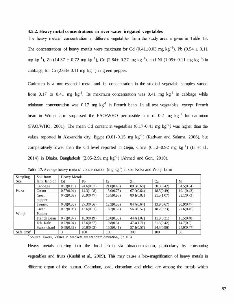
Table 17. Heavy Metals’ Concentration in soil at Koka and Wonji farm .....................................84
Table 18. Concentration of heavy metals (mg kg−1) in vegetables grown at Koka and Wonji
Farm ...................................................................................................................................86
Table 19. Inter-metal Pearson’s correlation of vegetable field soils .............................................88
Page 12
XII
Table 20. Transfer factor of heavy metals for different vegetables grown at Koka and Wonji
farm ....................................................................................................................................88
Table 21. DIM (mg kg−1 day−1) and HQ for individual heavy metals caused by the consumption
of different selected vegetables.....................................................................................91
Table 22. Principal component loadings of 19 variables in the Awash River water samples ......94
Page 13
XIII
LIST OF FIGURES
Figure 1. Nitrogen cycle in nature………………………………………………………………14
Figure 2. Phosphorus cycle in nature……………………………………………………………21
Figure 3. Map of the study area with water and sediment sample sites…………………………39
Figure 4. Map of the study area with soil and vegetable sample sites…………………………..40
Figure 5. Map of the study area from the Google Earth………………………………………..40
Figure 6. Trends of NO3-N, NO2-N, NH4-N and TN at different sampling points during dry
season…………………………………………………………………………………….59
Figure 7. Trends of DO, BOD and COD at different sampling points during dry season……...60
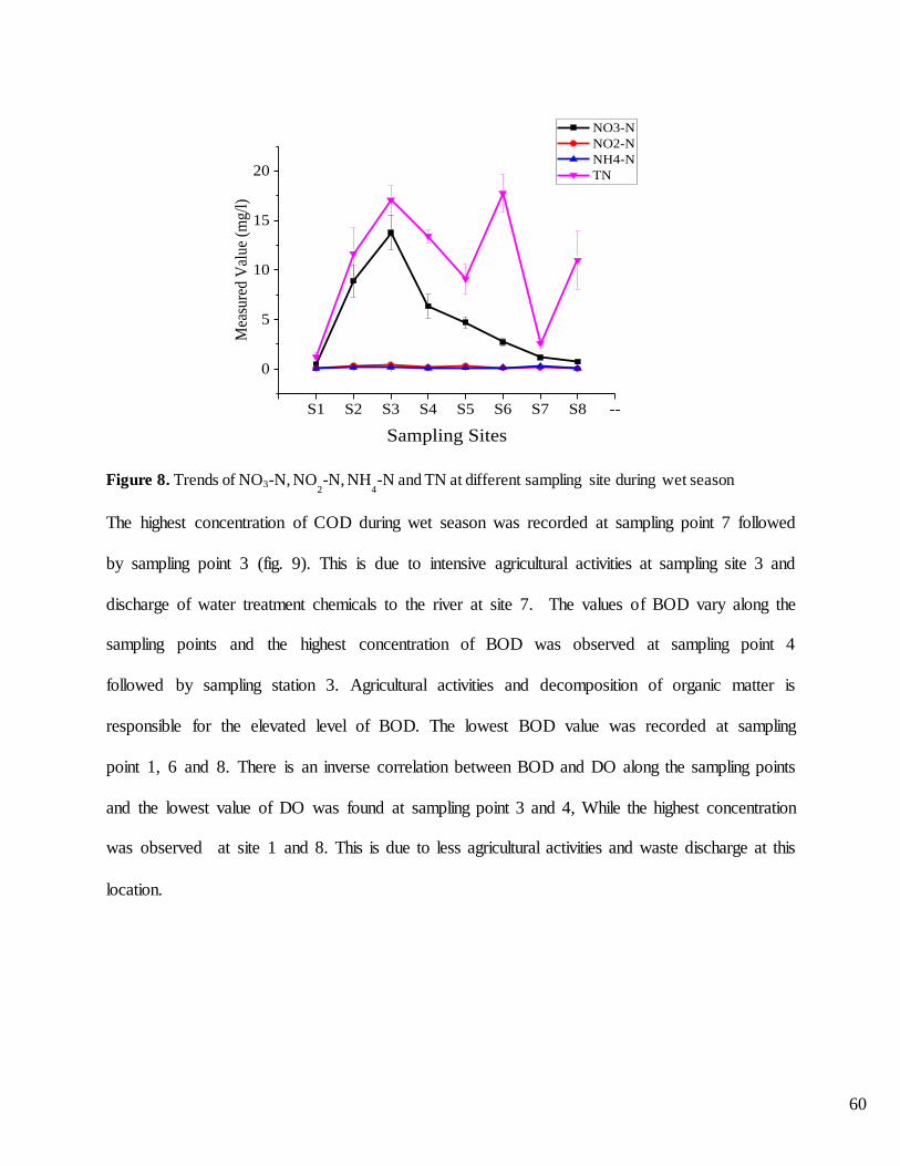
Figure 8. Trends of NO3-N, NO2-N, NH
4-N and TN at different sampling site during wet
season…………………………………………………………………………………….61
Figure 9. Trends of DO, BOD and COD at different sampling site during wet season…………62
Figure 10. Heavy metal concentration during dry and wet season……………………………...69
Figure 11. Mean Concentration of Heavy Metal in Vegetables of Wonji Gefersa, Ethiopia…...79
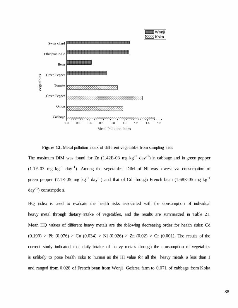
Figure 12. Metal pollution index of different vegetables from sampling sites………………….90
Figure 13a.The scree plot of the eigenvalues of principal components for dry season…………92
Figure. 13b. The scree plot of the eigenvalues of principal components for wet season……….92
Figure 14. Biplot of a standardized PCA-analysis performed on the physicochemical
and heavy metal parameters of Awash River during dry season………………………...95
Figure 15. Biplot of a standardized PCA-analysis performed on the physicochemical and heavy
metal parameters of Awash River during wet season……………………………………96
Figure 16. Dendrogram showing clustering of sampling sites on Awash River during dry
season…………………………………………………………………………………….97
Figure 17. Dendrogram showing clustering of sampling sites on Awash River during wet
season…………………………………………………………………………………….98
Page 14
XIV
LIST OF APPENDICES
Appendix 1: Scientific papers published from the dissertation............................................... 144
Appendix 2: Mean Value of Physico-chemical water quality parameters at different locations
of the Awash River during dry season .................................................................................... 145
Appendix 3: Mean Value of Physico-chemical water quality parameters at different locations
of the Awash River during wet season.................................................................................... 146
Appendix 4: Mean Concentration of heavy metals in Awash River during dry season ........ 146
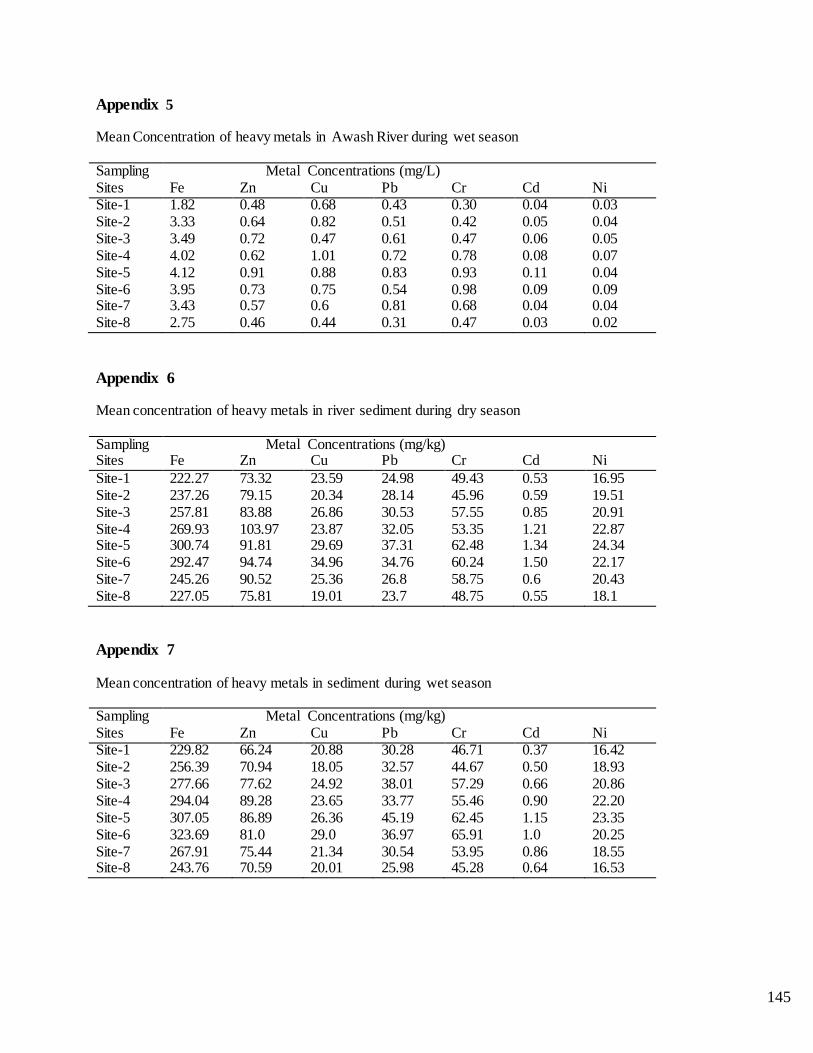
Appendix 5: Mean Concentration of heavy metals in Awash River during wet season ......... 147
Appendix 6: Mean concentration of heavy metals in river sediment during dry season ........ 147
Appendix 7: Mean concentration of heavy metals in sediment during wet season ................ 147
Appendix 8: Mean value of Heavy metals in paper wastewater ............................................. 148
Appendix 9: Mean value of heavy metals (μg/kg) in vegetables grown using paper wastewater
................................................................................................................................................. 148
Appendix 10: Mean value of heavy metals (mg kg-1) in soil of the study area ...................... 148
Appendix 11: Mean value of heavy metals (mg kg-1) in vegetables at Koka and Wonji farm...149
Page 15
XV
ACRONYMS AND ABBREVIATIONS
AAEPA Addis Ababa Environmental Protection Authority
AAS Atomic Absorption Spectrophotometer
ANOVA Analysis of Variance
APHA American Public Health Association
BOD Biological Oxygen Demand
COD Chemical Oxygen Demand
DIM Daily Intake of Metal
DO Dissolved Oxygen
EC Electrical Conductivity
FAO Food and Agricultural Organization
HI Hazard Index
HQ Hazard Quotient
MPI Metal Pollution Index
NTU Nephlometric Turbidity Units
RfDo Oral Reference Dose
TF Transfer Factor
THQ Target Hazard Quotient
TN Total Nitrogen
TP Total Phosphorus
USEPA United State Environmental Protection Agency
WHO World Health Organization
WT Water Temperature
Page 16
1
1. INTRODUCTION
In recent years, surface water pollution has received much attention worldwide. Both natural
processes and anthropogenic activities, like hydrological features, climate change, precipitation,
agricultural land use, and sewage discharge are the causes of deterioration of surface water
quality (Ravichandran, 2003; Gantidis et al., 2007; Arain et al., 2008).
Surface water, particularly rivers have various uses in different sector like agriculture, industry,
transportation, and public water supply. Nevertheless, Rivers have also been used for cleaning
and disposal purposes. This practices more pronounced in developing country, particularly in
Africa. Large amount of wastes from industry, domestic sewage and agricultural practices enter
into rivers which lead to worsening of water quality (Ravindra et al., 2003). Rivers are among
the major susceptible water bodies to pollution due to distant flow to carrying out municipal and
industrial wastes and agro-chemicals through runoff (Singh et al., 2005).
Surface water quality in different places is mainly influenced by both natural processes
(precipitation, weathering process and hydrological features) and anthropogenic activities like
domestic and industrial activities and agricultural land use (Varol et al., 2011). Domestic and
industrial waste discharge is a point source of pollution, while surface runoff is a seasonal
phenomenon which is mainly influenced by the climatic condition within the region (Singh et
al., 2004). River water pollution and concentration of contaminant varies with season due to the
changing pattern of precipitation and surface runoff (Vega et al., 1998).
Nutrient concentrations in rivers have been largely correlated with land use practice and change
of gradients (Howarth et al., 1988). Point and non-point source of pollution particularly from
anthropogenic activities are the main causes for nutrient enrichment of aquatic environment.
Point sources of nutrients include municipal and industrial wastewater discharge and runoff
Page 17
2
sewer discharge. In contrast to point sources of nutrients that is comparatively easy to monitor
and regulate, nonpoint sources like agricultural fertilizers, animal manure, and agricultural runoff
indicate more spatial and seasonal variability (Capone and Kiene, 1988).
Surface water pollution by heavy metals is the main problem because of their toxicity,
persistence nature in the environment and bio-accumulation effect (Cook, 1990; Sin, 2001).
Heavy metals discharge into a river from diverse sources; either natural or anthropogenic
(Adaikpoh., 2005; Akoto, 2008). Generally in non-polluted environments, the concentration of
heavy metals in rivers is not significant and mainly come from weathering of rock and soil (Reza
and Singh, 2010). The major anthropogenic sources of heavy metal in river water are untreated
industrial effluents, mining and smelting activities, sewage and agro-chemicals from agricultural
fields (Macklin, 2006; Nouri et al., 2008; Reza and Singh, 2010).
Heavy metals do not occur in soluble forms for a long time in waters; they are present mainly as
suspended colloids or are fixed by organic and mineral substances (Kabata-Pendias and Pendias
2001). Sediments are a major sinks for different pollutants such as heavy metals (Eimers et al.,
2001; Ho et al., 2003; Ikem et al., 2003) and also play a significant role in the assessment of
heavy metal pollution (Gangaiya et al., 2001).
Soils serve as the main sink for heavy metal pollutants in terrestrial ecosystems (Li et al., 2013)
and soil pollution by heavy metal is a worldwide problem (Liu et al., 2014). Commonly heavy
metals originate from two primary sources: natural background sources and anthropogenic inputs
including metalliferous mining and industries, agrochemicals and mineral fertilizers, vehicle
exhaust, sewage sludge and industrial wastes (Zhang, 2006). High concentrations of heavy
metals in surface soil can threaten human health via inhalation, ingestion and dermal contact
absorption (Sun et al., 2010; Xie et al., 2011). Heavy metals in deep soil may cause groundwater
Page 18
3
pollution (Camobreco et al., 1996; Richards et al., 1998). Soil heavy metal pollution
characteristics and ecological risks are the basis of soil environmental quality assessment. Once
heavy metals are deposited in the soil, they are not degraded and persist in the environment for a
long time and cause serious environmental pollution (Oyelola and Baatunde, 2008; Bora et al.,
2013).
Wastewater carries appreciable amounts of trace toxic metals which often lead to degradation of
soil health and contamination of a food chain, mainly through the vegetable grown on such soils
(Rattan et al., 2002). The toxic elements accumulated in the organic matter in soils are taken up
by growing plants and lastly exposing humans to this contamination (Khan et al., 2008).
Toxic heavy metals entering the ecosystem may lead to bioaccumulation, particularly by eating
fruits and vegetables (Kashif et al., 2009). This may cause an excessive buildup of heavy metals
in the body. Some heavy metals that are most often found to be responsible for harmful damage
to humans are Pb, Cd, Cr, Co and Ni (Gupta et al., 2008). Some heavy metals such as copper,
iron, zinc and manganese, are necessary to the body but in case of overexposure, they can lead to
heavy metal toxicity symptoms. Heavy metal concentrations vary among different vegetables,
which may be attributed to a differential absorption capacity of vegetables for different heavy
metals (Singh et al., 2010).
Heavy metals are among the major contaminants of vegetables. They are not biodegradable, have
been long biological half-lives and have the potential for accumulation in the different body
organs leading to unwanted effects (Nabulo et al., 2011; Singh et al., 2010).
Food is the major intake source of toxic metals by human beings. Among food system,
vegetables are the most exposed food to environmental pollution due to aerial burden.
Page 19
4
Vegetables take up heavy metals and accumulate them in their edible and non-edible parts at
quantities high enough to cause clinical problems to both animals and human beings. Excessive
content of metals beyond Maximum Permissible level (MPL) leads to number of nervous,
cardiovascular, renal, neurological impairment as well as bone diseases and several other health
disorders (WHO, 1992; Steenland and Boffetta, 2000; Jarup, 2003).
1.1 Statement of the problem
In Ethiopia, water and soil pollution is a major concern due to human population growth and
expansion of different industries. Various studies showed that all types of domestic wastewater
and more than 90% of the industries in the country release their effluents without any treatments
into the nearby agricultural farms and water bodies (AAEPA, 2007). This practice leads
environmental, health and economic burden in the country.
Among the major rivers in Ethiopia, Awash River which flows from the central highlands
through Ethiopia’s major industrial and agro-industrial belt is absorbing most domestic,
agricultural and industrial wastes (Shaka, 2015). Most of the existing industries and major towns
with in the upper watershed have no treatment plants for the discharge of their wastes and are
seriously polluting the water course (Melkame and Kasahun, 2013).
Moreover, the Modjo River, which is highly polluted by discharging effluent from the modjo
tannery industry and waste disposed from the town, is the main tributary of Awash River.
Besides this, the expansion of new industries and disposal of industrial wastes to the Awash
River is of great concern to the nation (Girma, 2001). Furthermore, food and beverage factories
tend to discharge heavy organic pollutants and dyes from textile factories are also released into
the same river.
Page 20
5
In view of persistent nature and cumulative behavior as well as the consumption of vegetables
and fruits, there is a need to test and analyze food items to ensure that the levels of these
contaminants meet the agreed international requirements. Regular survey and monitoring
programmes of the concentration of heavy metals in food products have been carried out for
decades in most developed countries (Sobukola et al., 2010). However, in developing countries
like Ethiopia, limited data are available on heavy metals in food products. Some data have been
reported for leafy vegetables (Fisseha, 2002).
In the study area the vegetables grown using Modjo and Awash River, which receives effluents
from upper stream towns and tanneries, for irrigation. Most of these vegetables cultivated in the
two farms are supplied to the vegetable market in Addis Ababa, Adama, Modjo town and the rest
enter into the nearby community with low price.
Although there was few research works has been undertaken on Awash River water quality
focusing on Physico-chemical parameters (Fasil Degefu, 2013; Shaka Nugusu, 2015; Amare
Shiberu et al., 2017a, b), there has not been any work done on pollution status of Awash River in
terms of space and season. The aim of this study was, therefore, to evaluate pollution status of
Awash River in terms of space and season and to assess the levels of different heavy metals in
edible portions of vegetables and the health risk associated with dietary intake.
1.2 Research question
What is the status of Awash River in terms of inorganic nutrient concentration?
What is the status of heavy metals in river water, wastewater, sediment, soil and vegetables in
the study area?
Is there a variation of nutrient and heavy metal level in Awash River in space and season?
Is there health hazard associated with dietary intake of vegetables in the study area?
Page 21
6
1.3 Objectives of the study
1.3.1 General objective
The general objective of this research is to assess pollution status of Awash River and level of
heavy metals in soil, vegetables grown at Wonji and Koka Farmlands
1.3.2 Specific Objectives
To determine the concentration of inorganic nutrient in Awash river
To determine the concentration level of heavy metals in river water, wastewater,
sediment, soil and vegetables in the area
To obtain trends in spatial and seasonal variation of heavy metals and inorganic nutrient
in Awash River
To estimate the potential health hazard associated with the heavy metal residue with
regard to consumers
Page 22
7
2. LITERATURE REVIEW
2.1. Physco-chemical parameters
Monitoring of river water quality can be carried out through determining the physical as well as
the chemical parameters. Various researches have been done in the past to investigate the
physico-chemical parameters of different rivers.
The physico-chemical parameters of Elala River in Tigray in the northern part of Ethiopia were
analyzed by Ftsum et al. (2015). They evaluated different parameters like electrical conductivity,
turbidity, chemical oxygen demand, nitrate nitrogen and total phosphorus. The study discovered
that the standards of these parameters were more than the prescribed limit of WHO guidelines
for drinking purposes. Likewise Ahammed et al. (2016) conducted a study to investigate the
water quality of Burigang River in Bangladesh. The process of sample collection was done in
summer, winter and autumn. The total of 30 water samples were collected and analyzed for 10
different water quality parameters. The results indicated highest level of turbidity, nitrate,
phosphate, DO, BOD and COD in the river.
Joseph and Jacob (2010) analyzed the physico-chemical characteristic of Pennar River in
Kerelato. The physical characteristics of water, such as, temperature, odour, colour, and
electrical conductivity were considered. Moreover, the purity of water was assessed by reviewing
total suspended solids (TSS), total dissolved substances (TDS) and total solids (TS) in water
samples taken. The physico-chemical parameters, such as, turbidity, pH, dissolved oxygen,
biological oxygen demand, chemical oxygen demand, phosphate and nitrate were also studied.
For the purpose of analysis, samples were extracted from 4 different locations in all seasons of
the year, viz. rainy, winter and summer. The results indicated that the river is highly polluted and
the water is unsuitable for drinking.
Page 23
8
Osman and Kloas (2010) carried out a research to evaluate the quality of Nile River at Aswan
and its estuaries at Rosetta and Damieetta, Egypt, for physico-chemical parameters like
conductivity, COD, DO, ammonia, nitrates and sulphates, and were found to be higher mean
values at the selected site than other locations. This was due to input of large amount of waste
water from industries, domestic as well as diffuses agricultural wastewater containing high
concentration of organic and inorganic pollutants.
Adeyemo et al. (2008) performed spatio-temporal pollution status of the rivers of Ibadan,
Nigeria. The water samples were collected from upstream and downstream of the rivers in the
major eleven sampling sites from October 2003 to September 2004. The parameters that were
assessed were DO, BOD, pH, chlorides, nitrates and phosphates. Varying levels of pollution
from clean to extremely-polluted were found during the different seasons, causing a risk to the
aquatic biodiversity.
Gupta et al. (2011) studied the physico-chemical analysis of the Chambal River water in Kota
city, India during the pre-monsoon season of the years 2007 to 2009. The finding indicated that
the pH, total hardness, alkalinity, chlorides, sulphates and total dissolved solids were found to be
in permissible limits. The presence of iron, ammonia and comparatively lower value of dissolved
oxygen indicate the river is polluted to some extent. In generally the river was moderately
polluted and highly polluted at the points of inflow of sewage and domestic wastes.
Kori et al. (2011) were assessed the Water Quality Index of Karanja River at Bidar District,
Karnataka. The water samples were collected from five sampling stations along the river during
December 2007 to November 2009. The physico-chemical parameters of the samples were
determined and a weighted arithmetic technique was used to compute the water quality index.
Page 24
9
The season based of the water quality index varies 66.16 to 81.88. As a result, the quality of
water is poor and water quality management is needed to prevent further degradation.
Chopra et al. (2012) conducted a research on the limnochemical characteristics of the Yamuna
River at upstream, downstream and at the point of inflow of industrial discharge and domestic
waste. Their studies indicated that the intensity of pollution increased at the point of
effluent/sewage disposal resulting severe pollution. Therefore, effluent/sewage should be treated
before discharging into the river. Similarly, Shrivastava et al. (2012) conducted the study on the
sewage disposal into the Mancha River in Betul City, Madhya Pradesh. The water samples were
collected from nine different sewage inlets during pre-monsoon, monsoon and post-monsoon of
2009. They were evaluated water quality for physico-chemical parameters like DO, COD, BOD,
chlorides and nitrates. The result revealed that all of the parameters were beyond the
recommended limits set by WHO.
Ugwu et al. (2012) evaluated the impact of growing population in the city of Abuja in Nigeria by
assessing the seasonal physicohemical characteristics of the Usma River. The study revealed that
all parameters measured were within the permissible level except total suspended solid, which
exceeded for all seasons. The values for electrical conductivity and total dissolved solids
indicated that the anthropogenic activities are on the increase in the area of study the increasing
pollution. Correspondingly, Sharma et al. (2012) performed an evaluation of the
physicochemical parameters of the Narmada River, Madhya Pradesh. The water samples were
collected monthly from three different sites along the river of a period of one year from August
2009 to July 2010. The different parameters characterized were pH, temperature, transparency,
DO, BOD, chlorides, phosphates, nitrate, alkalinity, sulphates and total hardness. The result
showed that phosphate, nitrate, alkalinity and sulphates were found to be high in September and
Page 25
10
October whereas pH, temperature, chlorides and total hardness were high in summer. The overall
values of the parameters were within the WHO limits.
Pollution levels of the water of the ―Irigu‖ River in Southern part of Kenya were assessed by
Ombaka and Gichumbi (2012). They evaluated both physicochemical and bacteriological
parameters, in order assess the quality of the River ―Irigu‖. They collected and analyzed the
water samples both in the summer and rainy season. In their assessment they found that certain
parameters like pH, turbidity and ammonia were raised during the dry seasons because of
anaerobic decomposition of organic matter. The phosphorous levels were above the limit which
was likely to enhance periodic flourish and eutrophication. The authors concluded that the river
waters could not be used for drinking as well as other domestic purposes.
Ashutosh et al. (2010) studied physico-chemical and biological parameters and their variability
in relation to the pollution of river water. The research finding showed that the polluted site
contained high values of chloride and COD and low value of dissolved oxygen, which indicates a
high pollution load. It was carried out greater impact of urban activity on the ground and river
water quality in Hoshangabad. Relatedly, Jain and Shrivastava (2014) studied comparative
review of physicochemical assessment of Pavana River. The study was aimed to review the
status of physicochemical characteristics of Pavana River, Pune. Comparative study of data of
water quality has been studied from 2005 to 2013 and the physicochemical parameter such as
pH, DO, COD, BOD has been compared.
The river water of Walgamo in Addis Ababa, Ethiopia was analyzed by Dessalew et al. (2017).
They checked the physicochemical properties of the water during dry and rainy season by taking
water samples at six points. A variety of parameters, such as, pH, WT, TSS, TDS, TP, NH4-N,
NO3-N, DO, BOD and COD were examined. The study discovered that the standards of BOD,
Page 26
11
COD and electric conductivity were more than the permissible limits of WHO. Comparably,
Erick et al. (2016) carried out study of physico-chemical characteristics of Ngong River, Kenya.
They assessed physical characters like temperature, pH, electrical conductivity, turbidity and
dissolved oxygen. In the observation, they found the pH in the range from 6.42-6.96, the EC
value was in the range of 425-865 μS cm-1 and turbidity values were between 68 – 85.27 NTU.
They revealed that the river water indicate some pollution.
Xu et al. (2012) analyzed the spatio-temporal variation analysis of water quality in the
Zhangweinan River, China. The study assessed different physico-chemical parameters like
electrical conductivity (EC), dissolved oxygen (DO), chemical oxygen demand (COD),
biological oxygen demand (BOD), total hardness (TH), total suspended solids (TSS), Chloride
(Cl-), Sulphate (SO42-), total nitrogen (TN), ammonia nitrogen (NH4-N), nitrate nitrogen (NO3-N)
and total phosphorus (TP). The results stated that the water pollution in this region is serious.
Likewise, the water quality of Zik River was investigated by Ewemoje and Ihuoma (2014). They
collected water samples of the River by sampling at five stations during May to July for physico-
chemical analysis. The physico-chemical parameters tested were: pH, biochemical oxygen
demand (BOD), dissolved oxygen (DO), electrical conductivity (EC), total suspended solids
(TSS) and Nitrate. This study showed that sewage discharge into River Zik have seriously
contributed to the pollution of the stream to levels which pose health and environmental hazards
to those using it downstream for domestic and agricultural purposes.
2.2. Nitrogen cycling
Nitrogen (N) is essential for all living organism and is a naturally occurring constituent in
freshwater systems, nevertheless, the anthropogenic demand for higher concentrations of
nitrogen to aid plant and crop production has caused in excess nitrogen entering freshwater
Page 27
12
systems, either via point source or from diffuse source through agricultural runoff (McArthur et
al., 2010; Parfitt et al., 2012). Worldwide, the use of nitrate-based fertilizers has gradually
increased since the 1950s and subsequently there has been a substantial increase in the amount of
nitrate within rivers (Meybeck, 1993a).
Nitrogen has many different forms: organic, inorganic, particulate, and dissolved. The organic
constituents of nitrogen are of importance since they represent the amount of nitrogen that is
available for biochemical processes. However, the organic forms of nitrogen are rarely
considered in the monitoring of water quality, because they are not as immediately biologically
available for uptake as the inorganic forms (Seitzinger and Sanders, 1997) and thus do not
promote excessive growth of algae when present in excess concentrations. Normally the
fractions of nitrogen measured in regards to water quality are total nitrogen (TN) and the
inorganic species, ammonium (NH4), nitrate (NO3), and nitrite (NO2).
Nitrogen is continually cycling through the atmosphere, hydrosphere, biosphere and lithosphere
in one of two ways, through fast biological cycles, or a slow geological cycle (Bolin et al., 1983).
The slow cycle represents that nitrogen is stored in minerals and rocks and is cycled slowly over
time through the atmosphere, hydrosphere, in earth’s crust and mantle (Johnson and Goldblatt,
2015). Nitrogen can exist in different forms within various rock type, i.e. mantle and meteorites
contain nitride minerals, while nitrate is found in silicate minerals, however, the concentration of
nitrogen is difficult to determine because of lack of standardized methods (Holloway and
Dahlgren, 2002). Current research has discovered that nitrogen can be found in concentrations
ranging from 1 mg l-1 to 1000 mg l-1 of N within rocks and sediment (Johnson and Goldblatt,
2015). Nitrogen is not a significant constituent of bedrock nonetheless, the nitrogen stored in the
Page 28
13
lithosphere is unavailable for living organisms and is released through the burning fossil fuels
(Diack, 2015).
The biological nitrogen cycle refers to the faster cycling of nitrogen from the atmosphere into the
hydrosphere and biosphere. Dinitrogen gas (N2) is a main component of the atmosphere,
accounting for 78% of the atmospheric gases and so N2 is involved by nitrogen fixation (Follet,
2001). Nitrogen fixation occurs when microorganisms, which have a symbiotic relationship with
herbaceous plant species like legumes, convert the nitrogen gas to bioavailable forms of nitrogen
(Vitousek et al., 1997). Once drawn into the soil nitrification, i.e. bacterial oxidation takes place
which convert the biologically available forms of ammonium (NH4+) to nitrate (NO3
-) (Deek et
al., 2010). Organic forms of nitrogen in the soil are converted, by soil microbes via
ammonification, to inorganic forms, and from inorganic forms to organic via immobilization
(Follett, 2001; Sauer et al., 2001). Both forms are available for plant uptake and used in
photosynthesis. Nitrogen from the biosphere can be converted through denitrification and
returned to the atmosphere as nitrogen gas (N2), ammonia gas (NH3), or nitrous oxides (NO, N2O
and NO2) (Sauer et al., 2001). Ammonia within the nitrogen cycle also forms as a by-product of
urea, microbial decomposition and soil processes.
Nitrogen is largely soluble and a vital component in most fertilizers added to agricultural
production areas and horticulture (Chand et al., 2006). During high runoff period excess NO3- is
flushed from the soil directly reach to surface water or percolates into groundwater sources. Due
to its high solubility, NH3 in the atmosphere is quickly scavenged into precipitation and reduces
to ammonium when in solution (Follett, 2001). However, ammonium (NH4+) readily binds to any
negatively charged clay present (Diack, 2015), so that soils that have low clay content may be
more vulnerable to ammonium leaching into waterways. On the other hand, as nitrate is
Page 29
14
negatively charged it is repelled by clay soil particles, as a result allowing more excess nitrate to
build up in aquatic environment (Follett, 2001). The buildup of nitrate and ammonium within
watercourse, along with phosphorous, creates suitable environment for the primary production in
aquatic ecosystems, and consequently eutrophication and toxic algae blooms more pronounced
(Keeney and Hatfield, 2001).
Figure 1. Nitrogen Cycle in nature, Fountain (2010).
2.2.1. Nitrogen fixation
Nitrogen fixation is a bacterially mediated, exergonic reduction process which converts
molecular nitrogen to ammonia:
8H+ + N2 + 8e- 2NH3 + H2
On annual basis, total nitrogen fixation in aquatic systems rarely exceeded 20 Kg N ha-1 (Ghaly
and Ramakrishnan, 2015). In general, N fixation requires adenosine triphosphate (ATP) which
Page 30
15
is generated by photosynthesis; so this process is inefficient at night. However, cynobacteria can
fix nitrogen directly, so do not have this diurnal limitation (Sprent, 1987).
2.2.2. Ammonification or mineralization
Ammonium production occurs both in the water column of rivers and lakes in their sediments.
Microbial decompostion converts organic nitrogen to ammonical form. This process is oxygen-
demanding and regenerates available nitrogen for re-assimilation by primary producers.
Ammonification can result in rapid nitrogen cycling between the sediment and the water
column. The rate of release of nitrogen from decomposing organic matter can be an important
factror in determining nutrient limitation in fresh waters. Where nitrogen release is relatively
slow, the process of assimilation can become N-limited.
Ammonia in fresh waters can exist as the ammonium cation (NH4+) or as un-ionized ammonia
molecule (NH3). High temperature and high pH (pH > 8) encourage the conversion of
ammonium to ammonia. Ammonia (NH3) is more toxic than ammonium, and acute toxicity can
occur at low concentrations. Fortunately, high concentration of ammonia are usually only
associated with wastewater discharges where biological treatment is minimum (Jetten, 2001).
2.2.3. Nitrification
Nitrification is a two stage oxidation process mediated by the chemoautotrophic genera.
Nitrosomonas (NH4+ to NO2
-) and Nitrobacter (NO2- to NO3
-). In this exothermic reaction, more
energy for biosyntesis is obtained from the oxidation of NH4+ to NO2
- ( -84 kcal mole-1) than the
subsequent oxidation to NO3- ( -18 kcal mole-1). The net reaction is:
NH4+ + 2O2 -- NO3
- + H2O + 2H+
Page 31
16
The oxidation of ammonia to nitrite by Nitrosomonas is usually rate-limiting, so nitrite is rarely
present in appreciable concentrations in fresh waters. Nitrate, the end product, is highly
oxidized, soluble and biologically avaialable.
The nitrifying bacteria also pH and temperature susceptible, with an optimum pH of 8.4 – 8.6
(Wild et al., 1991) and requiring a temperature above 150C. Nitrosomonas has a wider
temperature tolerance than Nitrobacter, and the growth rate constant for these bacteria increases
by approximately 10% per degree celsius up to about 250C.
A high rate of nitrification is essential for efficient N cycling in fresh waters, particularly as
nitrate is an important substrate for denitrification. Chemoautotrophic nitrifying bacteria are
usually dominant in fresh waters and their activity is generally highest at the sediment- water
interface where NH4–N generation is maximum (Reyes et al., 2017). Howerver, in eutrophic
waters in particular, nitrate generated internally through nitrification is often relatively
unimportant in comparison with the nitrate load received from the environment. Nitrification is
often high during summer when water temperatures are high. During this period, catchment
inputs are often minimum and algal utilisation of nitrogen is maximun. Nitrification during this
period could be critical to the efficient cycling of nitrogen within the aquatic system.
2.2.4. Denitrification
Loss of nitrate from river systems can occur through denitrification or dissimilatory nitrate
reduction. Denitrification is quantitatively more important, particularly in river and lake
sediments, and is high in summer months (Royal Society, 1983). The rate and extent of
denitrification is controlled by the oxygen supply and available energy provoded by organic
matter. It is an important mechanism in the reduction of nitrate concentrations in reserviors, but
Page 32
17
is limited by the requirement for anaerobic conditions and a fixed bacterial carbon supply
(Bonete et al. 2008).
[
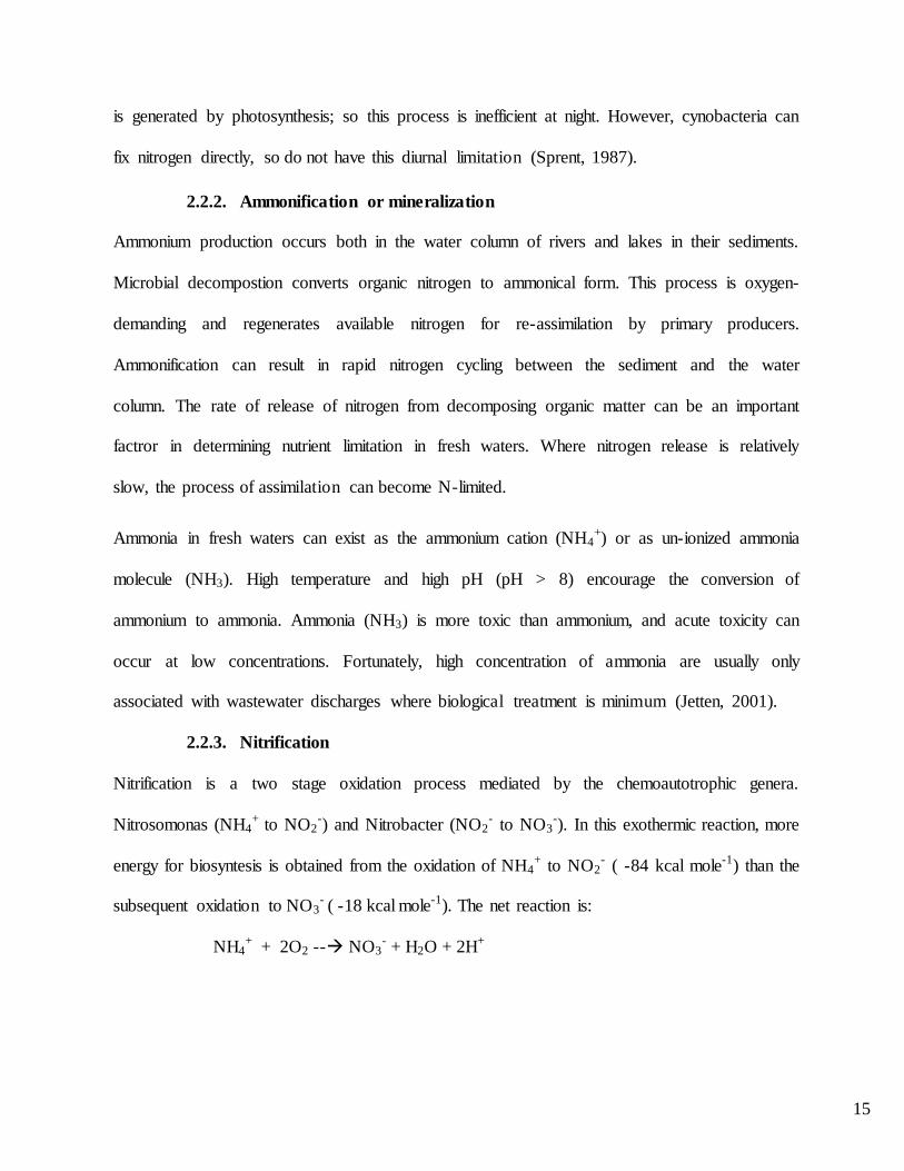
2.3. Phosphorus cycling
Phosphorus (P), like nitrogen, is vital for all living organisms. It plays a substantial role in the
metabolism, photosynthesis, and growth of plant species (Vilmin et al., 2015). Naturally
phosphorus is derived from rock weathering, moreover it is found within the atmosphere and
vegetation (Withers and Jarvie, 2008). The hydrological cycle acts as one of the major driving
forces for transporting phosphorus from terrestrial to freshwater environment, as precipitation
and runoff provide energy for phosphorus movement and mobilization (Leinweber et al., 2002).
The cycling of phosphorus comprises a range of physico-chemical processes that are influenced
by different factors like catchment hydrology, chemistry, and lithology, resulting of a complex
cycle (Caraco, 2009). In river water, phosphorus usually exists as orthophosphate molecule, its
most oxidized form. In the global perspective the cycling of phosphorus is covers a large
distance, and transporting across a wide scale from 100 – 1000s of km (Caraco, 2009), where
rivers play a crucial role in transferring phosphorus from terrestrial environment to aquatic
ecosystem. At the catchment scale phosphorus cycling is a slow process since phosphorus does
not have a gaseous state (Fountain, 2010; Caraco, 2009), and is closely cycled through the soils
(Leinweber et al., 2002; Richardson et al., 2004).
Inorganic phosphorus is stored within the soil and is easily available for plant uptake, plants then
convert the phosphorus to an organic form, as the plant matter then dies the organic phosphorus
is returned to the system in the form of inorganic phosphorus, as a result of mineralization during
decomposition, excretion, and enzyme breakdown (Baldwin et al., 2002; Leinweber et al., 2002;
McLaren and Cameron, 1996).
Page 33
18
In phosphorus cycling, the processes of absorption and desorption (phosphorus fixation) take
place between dissolved phosphorus and sediment bound phosphorus and encompasses various
environmental variables, like pH and the composition of organic matter (Leinweber et al., 2002;
Jones, 2004; Fountain, 2010). Soluble phosphorus reacts with the surface of the soil colloid but is
still available for uptake (Frost, 2004). Once absorbed the phosphorus is in a labile state and
mineralizes slowly (McLaren and Cameron, 1996). In contrast, sediment-bound phosphorus,
which can range from 1 nm (the soil colloid) to soil masses up to 10 mm in size, is mobilized or
eroded during precipitation period and leached into surface water (Doughterty et al., 2004).
In undisturbed freshwater environment phosphorus naturally occurs in very low concentrations,
making it a biologically limiting nutrient (Vilmain et al., 2015; Correll, 1998). Nevertheless, due
to the rapid urban area expansion and agricultural development, there has been an increase
enrichment of phosphorus in freshwater systems as a result of extensive use of anthropogenic-
derived phosphorus (Withers and Jarvie, 2008; Parkyn and Wilcock, 2004; Leinweber et al.,
2002).
The application of phosphorus based fertilizers to agricultural land has increase for soil fertility
and crop productivity. Various studies have reported the increased use of phosphorus-based
fertilizers with equivalent increasing level of phosphorus within freshwater systems (Woodward,
2013; Parkyn and Wilcock, 2004). The addition of phosphorus to the agricultural land causes
excessive amount of phosphorus accumulate within the top of the soil surface (McLaren and
Cameron, 1996; Fountain, 2010). As a result, during a rainfall event excess phosphorus is eroded
and leached from the soil and transported through overland flows and sub-surface pathways into
nearby rivers (McLaren and Cameron, 1996; Parkyn and Wilcock, 2004). Agricultural activity
also increases erosion and runoff causing an increased supply of suspended sediment to rivers
Page 34
19
(Parkyn and Wilcock, 2004). The phosphorus bound to soil particles once in a river can be lost
from the system to burial in the channel and riverbanks, but can also be easily remobilized under
high flow conditions (Bowes et al., 2003).
The phosphorus in the natural water body is provided by anthropogenic (industrial and
agricultural sources) and natural sources. The phosphorus increase is caused by domestic
wastewater (detergents and soaps, pesticides, food wastes, and human metabolic waste)
(Sommaruga et al., 1995; Berbeiri and Simona, 2001) food processing industries (meat,
vegetable, and cheese processing) (Tusseau-Vuillemin, 2001), distillery, synthetic and natural
(cow dung, pig dung, and poultry manure) fertilizers used in agro-ecosystem (Penelope and
Charles, 1992), agricultural runoff and domestic sewage, phosphate mines (Das, 1999).
The quantities of phosphorus entering the surface water vary with the amount of phosphorus in
catchment soils, topography, vegetative cover, quantity and duration of runoff flow, land use,
and pollution. In oceans, the concentration of phosphates is very low, particularly at the surface.
The reason lies partly within the solubility of aluminium and calcium phosphates, but in any case
in the oceans phosphate is quickly used up and falls into the deep sea as organic debris. There
can be more phosphate in rivers and lakes, resulting in excessive algae growth (USEPA, 1986).
Phosphorous is considered as biologically limiting nutrient, which means there is inadequate
phosphorus in the environment to support higher order species. On the other hand, when
phosphorus concentrations are increased, the excess phosphorus reached into freshwater
ecosystems is retained and used in biological processes (Correll, 1998). The excess of
phosphorus can then lead to increased primary productivity, high rates of decomposition, and
depletion of dissolved oxygen resulting in eutrophication (Novotny, 2003). Phosphorus
Page 35
20
enrichment, or states of eutrophication, can ultimately lead to environmental, economic, cultural,
and health related issues (Withers and Jarvie, 2008).
In aquatic environments phosphorus can be present in different forms: organic phosphorus (e.g.
sugars, nucleic acids and enzymes) or inorganic phosphorus (e.g. mineral sources like
orthophosphate and polyphosphate) (Vilmin et al., 2015). Particulate organic phosphorus is
comprised of organic matter, such as living or solid detrital matter, and dissolved organic
phosphorus is an intermediate state in which mineralization of solid organic matter is occurring
(Vilmin et al., 2015). Dissolved reactive phosphorus is the reactive portion of mineral dissolved
phosphorus, which is the only form of inorganic phosphorus that can be used by organisms
(Vilmin et al., 2015; Jarvie et al., 2002). When assessing water quality the fractions of
phosphorus commonly studied are dissolved phosphorus (PO43-) and total phosphorus (TP).
Dissolved reactive phosphorus is used as an indicator of the phosphorus that is available for
biological uptake, particularly the amount available allowing for nuisance algae growth and
eutrophication (Davies-Colley and Wilcock, 2004), while total phosphorus is an indicator of the
potential amount of phosphorus free for nutrient cycling and can also indicate the amount of
phosphorus lost by leaching (Leinweber et al., 2002).
Page 36
21
Figure 2. Phosphorus Cycles in nature, Fountain (2010).
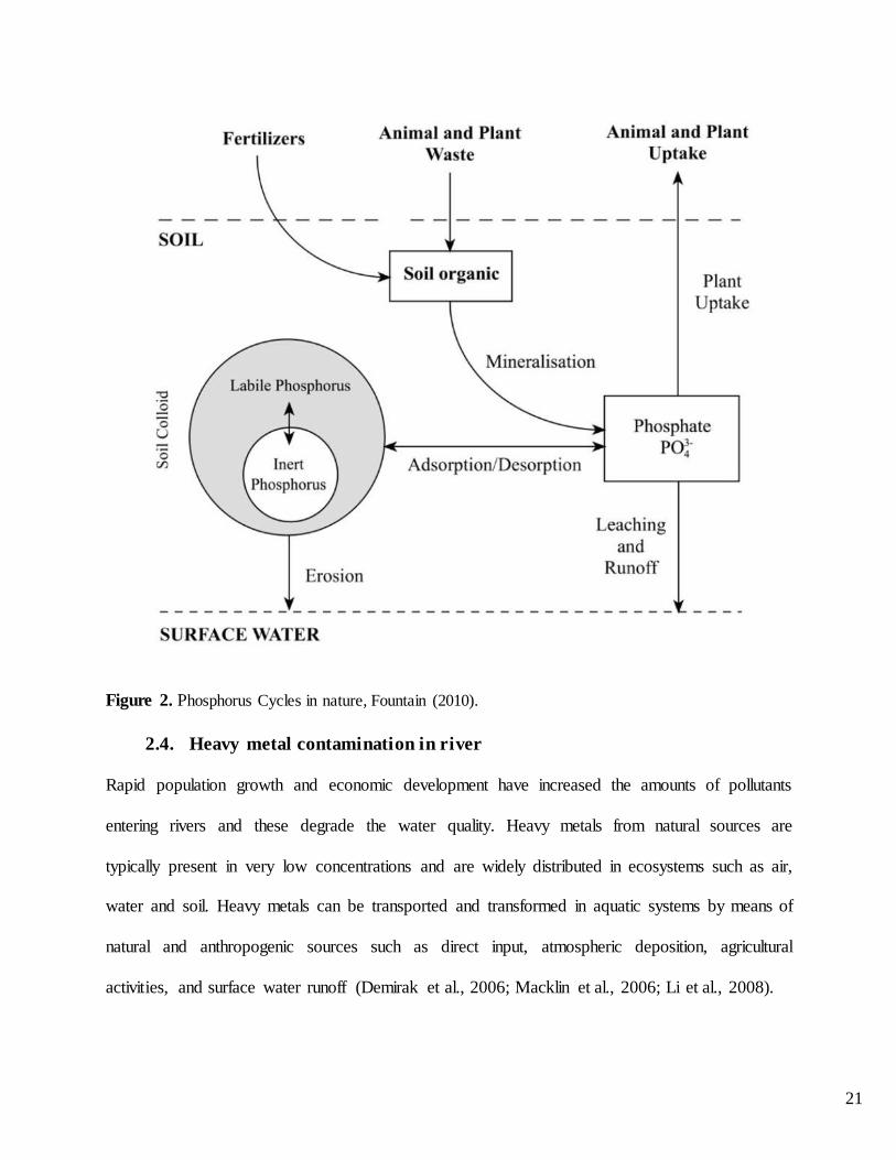
2.4. Heavy metal contamination in river Rapid population growth and economic development have increased the amounts of pollutants
entering rivers and these degrade the water quality. Heavy metals from natural sources are
typically present in very low concentrations and are widely distributed in ecosystems such as air,
water and soil. Heavy metals can be transported and transformed in aquatic systems by means of
natural and anthropogenic sources such as direct input, atmospheric deposition, agricultural
activities, and surface water runoff (Demirak et al., 2006; Macklin et al., 2006; Li et al., 2008).
Page 37
22
In areas where economic activities are intensive, such as industrial, agricultural and mining
locations, the heavy metal contamination is typically widespread. Therefore, heavy metal levels
can often exceed the natural background in aquatic environments (Bryan and Langston, 1992;
Obasohan et al., 2006). Although there are many types of river pollutants, heavy metals are of
greatest concern due to their slow decomposition under natural condition and their bio-
condensation by aquatic organisms (Sin et al., 2001; Li et al., 2008; Obasohan et al., 2008;
Rauf et al., 2009; Liu and Li, 2011; Varol, 2011).
Discharge of heavy metals into rivers or any other aquatic environment can change both aquatic
species diversity and ecosystems due to their toxicity and accumulative behavior (Al-Weher,
2008). Heavy metals dissolved in water also endanger the lives of the public who use it for
drinking and also irrigation. When used for irrigation heavy metals have the risk of being
incorporated in food chain and hence consumed by the human (Wogu and Okaka, 2011).
Many studies have been conducted globally on the heavy metals contamination in rivers.
Papafilippaki et al. (2008) examined the seasonal variations of copper, lead, chromium, zinc and
cadmium in the surface water of the Keritis River, Greece. The toxicity of these metals varies
considerably between the warm and the wet periods. Seasonal variations were attributed to
agricultural activities, wastewater discharges and the physico-chemistry of water, temperature,
flow rate, pH and redox conditions. The contamination of water with Cu, Cd, Pb, Cr and Zn was
positively correlated to the pH.
Pandey et al. (2010) investigated the mid-stream water quality of Ganga River, India. Twelve
sampling sites were identified along a 20 km stretch of the river. The following heavy metals
including Cd, Cr, Cu, Ni, Pb and Zn were analyzed in the laboratory by using wet acid digestion
method. The data revealed that the mid-stream water of the river Ganga at Varanasi is invariably
Page 38
23
contaminated by heavy metals. Highest concentrations of Cd, Cr, Ni, and Pb were recorded
during winter and that of Zn during summer season. The overall concentration of heavy metals in
water showed the trend: Zn> Ni> Cr> Pb> Cu> Cd. Moreover, Correlation analysis showed that
heavy metal concentration in mid-stream water had significant positive relationship with rate of
atmospheric deposition at respective sites. The mean levels of Cd, Ni, and Pb at three stations,
were above the recommended level of WHO so that the use of such water for drinking purpose
might be lead to potential health risk in long run. Similarly, the purity levels of the Huluka River
of Ambo region, Ethiopia were assessed by Prabu et al. (2011). The result conclusion was that
most parameters exceeded the limits and the water quality was found to worsen steadily, due to
the direct discharge of domestic and municipal sewage. It was also found that the water quality
deteriorates as one goes more downstream.
Amadi (2013) investigated pollution potential of heavy metals Sosiani River, in Kenya for dry
and wet season. Heavy metals like Cu, Zn, Pb, Cd and Fe were studied and among these Zn
concentration was above the WHO standards recommended for drinking water (0.50 ppm).
Discharge from the flower farm, leachates from the waste dumpsite, untreated wastewater from
industries seems to be the main source of heavy metal contamination. Likewise, Kumari et al.
(2013) characterized heavy metal content in Ganga Jal River. Water samples were collected from
six stations and analyzed Pb, Zn, Fe, Ni, Cr, Cd and Cu. The result indicated that Cu, Cd, Cr, Ni,
Fe, Pb, and Zn were the highest in summer and the lowest in monsoon season.
Pandey et al. (2014) investigated the seasonal changes in concentration of heavy metals in Ganga
River in Allahabad. Samples were collected at different sampling sites during summer, monsoon
and winter seasons in year 2013-2014. Atomic Absorption Spectroscopy (AAS) technique was
used to determine the concentration of four heavy metals i.e. Fe, Zn, Cr and Co in three seasons.
Page 39
24
Results showed that wide variations in the heavy metal levels varying from high concentration
during summer and low concentrations during winter season. The order of heavy metals
accumulation in the Ganga River was Fe>Zn>Cr>Co. Moreover, statistical data analysis carried
out through correlation methods and correlation coefficients were calculated between different
pairs of parameters to identify the highly correlated and interrelated water quality parameters.
Raghuvanshi et al. (2014) analyzed the water quality of River Ganga in Allahabad district. Water
samples were collected from five sampling sites in the year 2012-2013. Ten water quality
parameters for all the sites were estimated by adopting the standard methods and procedures. The
results revealed that the average pH value was measured as 8.07±0.44, electrical conductivity
was 188.49±63.00 μmho cm-1, Dissolved Oxygen was 6.47±0.82 mg/l, Biochemical Oxygen
Demand was 9.41±1.41 mg/l, Chemical Oxygen Demand was 15.28±3.07 mg/l, Total Hardness
was 118.56±40.91 mg/l, Total Alkalinity was 168.46±12.50 mg/l, Chloride was 27.49±16.97
mg/l and Total Dissolved Solids was 216.83±13.84 mg/l. Comparison of estimated values with
WHO standards revealed that the river water of study area is polluted which may be harmful for
aquatic species and human beings. Correlation coefficient showed highly significant positive and
negative relationship (p<0.05 level).
Lawal et al. (2014) in their work on heavy metal pollution level of Kampani River, Nigeria.
From their findings, highest concentration of Cr, Cd and Fe was recorded and all the metals
examined were above the acceptable limits set by WHO for drinking water. They claimed that
the use of charger batteries, application of fertilizer and pesticide on farmland are main sources
of heavy metal contamination. Correspondingly, Thomas and Mohaideen (2015) determine
heavy metals content in Korttalaiyar River, India. They reported that maximum heavy metal
concentrations in water are arsenic (0.03 mg/l), cadmium (0.022 mg/l), chromium (0.046 mg/l),
Page 40
25
lead (0.015 mg/l) and mercury (0.016 mg/l). The discharge of untreated effluent from various
industries and domestic sewage is the main source of pollution for Korttalaiyar River.
Vaishnavi and Gupta (2015) studied the levels of heavy metals in the river waters in and around
Pune City, Maharashtra, India. A total of nine water samples were collected from the river sites.
The samples were analyzed for the determination of different heavy metals (Cd, Co, Cr, Cu, Ni,
Pb and Zn). The result indicated that the mean concentrations of Cd and Pb obtained were 0.039
and 0.107 mg/l respectively which were higher than the permissible limits of WHO while, the
level of Cr, Mn, Zn, Ni and Mo is within the allowed WHO limits in drinking water.
2.5. Heavy metal contamination in sediments
Contamination of sediments by heavy metals is one of the main concerns to aquatic ecosystems.
Sediment represents one of ultimate sinks for heavy metals discharged into aquatic environment.
Consequently, sediment quality is a good indicator of pollution in water column, where it tends
to concentrate the heavy metals and other organic pollutants (Saeed and Shaker, 2008). Abraha et
al. (2012) observed that sediments play a substantial role in remobilization of pollutants in
aquatic systems under favorable conditions and interactions between water and sediments. Akan
et al. (2010) insist that sediments in rivers do not only play vital roles at influencing the
pollution, they also record the history of their pollution.
Heavy metals accumulate in sediments through complex physical and chemical adsorption
mechanisms depending on the nature of the sediment matrix and the properties of the adsorbed
compounds (Ankley et al., 1992). Heavy metals once adsorbed on the sediments are not freely
available for aquatic organisms under changing environmental conditions (temperature, pH,
redox potential, salinity) of the overlying water these toxic metals are released back to the
aqueous phase (Soares et al., 1999).
Page 41
26
The sediment play an important role as it has along residence time therefore is an important
source for the assessment of an anthropogenic contamination in rivers (Förstner and Wittman,
1983; Jain et al., 2005). Sediments capture hydrophobic chemical pollutants that enter water
bodies (McCready et al., 2006) and slowly release the contaminant back into the water column
(Chapman and Chapman 1996; McCready et al., 2006). Therefore, ensuring a good sediment
quality is vital to sustain a healthy of aquatic ecosystem, which ensures good protection of
human health and aquatic life.
Different researchers had been investigated the pollution status of heavy metals in sediments.
Milenkovic et al. (2005) determined the concentrations of As, Fe, Cr, Mn, Cu, Ni, Cd, Pb, Hg
and Zn in the sediments of River Danube and found that the range of mean concentrations of
heavy metals increased by 46.60% to 156.20% due to increased industrial effluent discharges in
the river. The toxicity of Cu, Cr, Ni, Zn and predominantly Cd in the sediments was higher than
the target values indicating potential risk to the ecosystem. Alike, Rafiu et al. (2007) determined
the concentrations of trace metals, Cd, Pb, Mn, Zn, Cu and Ni in surface water and sediments
along the Blaauwbankspruit stream, South Africa. This investigation revealed higher metallic
load in sediments than that of water due to wastewater discharge from sewage treatment plant
and effluents from a gold mine.
In Turkey, Ayas et al. (2007) conducted a study on the accumulation of Cd, Pb and Ni in water
and sediment samples. Results showed that spatial distribution of the three heavy metals was
extensive throughout the study area. In the water samples, heavy metal concentrations were
below the respective detection limits of the metals. Predictably, metal concentration levels in the
sediment samples were higher than that of the water samples. Similarly, the distribution and
enrichment of heavy metals (Cd, Cr, Cu, Mn, Pb, Ni and Zn) in sediments in the Tapacurá River
Page 42
27
basin, Brazil, were studied by Aprile and Bouvy (2008). They revealed that metal concentrations
in the industrial and agricultural areas were higher than those in the urban areas. Anthropogenic
influences were determinant factors controlling the spatial variations of heavy metals.
Beg and Ali (2008) assessed the sediment quality of Ganga River at Kanpur city where effluents
from tannery industries are discharged. Sediment samples from upstream and downstream area
were collected and analyzed for trace metals. The result showed that Cr in downstream sediment
was 30-fold higher than in upstream sediment and its concentration was above the probable
effect level.
Sharmin et al. (2010) investigated the heavy metals mobility pattern in sediments of the aquatic
ecosystem of Nomi River, Japan. The heavy metal mobility in the sediments was in the order: Cd
> Cu > Cr > Ni > Fe > Mn. The presence of different clay minerals was found to be the main
accumulation of heavy metals in sediments. Correspondingly, Akan et al. (2010) characterized
the level of Co, Pb, Cu, Cd, As, Ni, Mn, Fe, Pb and Cr contamination and the degree of river
sediment quality deterioration of Ngada River. The study revealed that heavy metals toxicity
increased considerably with increasing sediment depth, indicating age-long accumulation of
heavy metals as a result of anthropogenic sources and were higher than the WHO standard
sediment guideline limits exposing the aquatic food chain at high risk of persuade heavy metal
contamination.
Ye et al. (2012) investigated the accumulation of metals in sediments of the Pearl River, China.
Spatial distribution of metals was consistent with anthropogenic input into the river basin. In
terms of vertical deposition, there was a decline in pollution from the mid-1990s consistent with
efficient pollution management in the basin. Comparably, Shanbehzadeh et al. (2014) examined
heavy metal concentrations in water and sediment, upstream and downstream of the entry of the
Page 43
28
sewage to the Tembi River, Iran. The finding indicated that the average concentrations of the
metals in water and sediment in downstream sites were higher than that of the upstream sites.
Weber et al. (2013) investigated the level of heavy metals in sediment sample in Brazilian River.
It was observed from recorded results that concentrations of heavy metals were high in sediments
sample as compared to water samples. Agriculture activity and sewage sludge seems to be the
main source of heavy metal contamination. Similarly, Kihampa and Wenaty (2013) performed a
research on the contamination of Mara River sediment by heavy metals. The study assessed six
toxic heavy metals like Cd, Pb, Cu, Zn, Cr and Hg. The results stated that the concentration of
heavy metals in the river was above the recommended international and national limits for
drinking and irrigation waters. It was found out that discharge of mining to be the potential
source of the heavy metals in Mara River.
Sediment pollution by heavy metals in Ganga River was studied by Pandey and Singh (2015).
They observed that highest concentration of Fe (31,988.6 μg g-1) and Mn (372.0 μg g-1) in
sediment samples. It was confirmed that local sources like agricultural, untreated urban and
industrial wastewater are the main causes for pollution. Correspondingly, Edokpayi et al. (2016)
reported highest concentration of heavy metals in Mvudi River sediment, South Africa. It was
found that Cd, Cr and Cu were above sediment quality guidelines. Untreated wastewater, runoffs
from agricultural soil, landfill sites and atmospheric deposition are the dominant sources of
pollution in a river.
2.6. Soil pollution from heavy metals
Heavy metals occur at typical background in all ecosystems; however, anthropogenic releases
can result in higher concentrations of these metals relative to their normal background values
(Adeleken and Abegunde, 2011). Soils may become contaminated by the accumulation of heavy
Page 44
29
metals and metalloids through emissions from the rapidly expanding industrial areas, mine
tailings, disposal of high metal wastes, leaded gasoline and paints, land application of fertilizers,
animal manures, sewage sludge, pesticides, wastewater irrigation, coal combustion residues,
spillage of petrochemicals, and atmospheric deposition (Khan et al., 2008; Zhang et al., 2010).
Soils are the major sinks for heavy metals released into the environment by aforementioned
anthropogenic activities and unlike organic contaminants which are oxidized to carbon dioxide
by microbial action, most metals do not undergo microbial or chemical degradation
(Kirpichtchikova et al., 2006), and their total concentration in soils persists for a long time after
their introduction. Changes in their chemical forms (speciation) and bioavailability are, however,
possible (Adriano, 2003).
The fate and transport of a heavy metal in soil depends significantly on the chemical form and
speciation of the metal. Once in the soil, heavy metals are adsorbed by initial fast reactions
(minutes, hours), followed by slow adsorption reactions (days, years) and are, therefore,
redistributed into different chemical forms with varying bioavailability, mobility and toxicity
(Shiowatana et al., 2001; Buekers, 2007). This distribution is thought to be controlled by
reactions of heavy metals in soils such as (i) mineral precipitation and dissolution, (ii) ion
exchange, adsorption, and desorption, (iii) aqueous complexation, (iv) biological immobilization
and mobilization, and (v) plant uptake (Levy et al., 1992).
Various researches have been carried out on the heavy metals pollution in soils. Ahmad and Goni
(2010) in their study showed highest deposition of Fe and Zn around industrial areas in Dhaka,
Bangladesh. Long-term use in the production of machine tools, paints, pigments and alloying in
various industries are the major source of soil contamination by heavy metals. Similarly, Rapheal
and Adebayo (2011) reported that highest concentration of Pb, Cd, Cu and Zn metal in farmland
Page 45
30
soil. Fertilizer application and other organic manure applied to soils are the main cause of soil
contamination. It was suggested that the soil contamination may be considered when
concentrations of an element in soils were two-three times greater than the average background
levels.
Abraha et al. (2013) carried out study of heavy metal accumulation in the soil, vegetables and
toxicological assessment in Ethiopia. The results stated that four heavy metals (Mn, Zn, Cr, and
Cu) the concentration levels were higher. It was found out that the discharge of wastewater from
industries were the major causes for the higher concentrations of the metals.
Malan et al. (2015) investigated pollution potential of heavy metals in horticultural soil in South
Africa. The results indicated that maximum concentration of Cd and Cr which exceed the
maximum permissible concentrations in the winter cropping season. Intense agricultural
practices as well as pig, poultry and cattle farming are the main cause of soil pollution. Likewise,
Ye et al. (2015) studied the heavy metal content in the soil in Zhejiang province, China. Out of
202 agricultural soils being analyzed, 50 and 60 soil samples exceeded the maximum allowable
contents of Cd and Hg respectively. They revealed that the sources for soil pollution in the study
sites were industrial pollution, sewage irrigation and agro-chemical application.
Almasoud et al. (2015) conducted a research on heavy meal soil pollution due to industrial
activities in Saudi Arabia. They analyzed 56 soil samples from Jubail, which is one of the major
industrial cities in the Middle East. They studied Fe, Mn, Zn, Cu, Cr, Co, Ni, Pb and Cd and
found that higher Cr concentration and it was higher than the soil common range as well as the
geochemical background indicating industrial petrochemical pollution in the study area.
Correspondingly, Tawfiq and Ghazi (2017) assessed heavy metal pollution in the soil and its
influence in Iraq. For the investigation they collected 36 soil samples in Maysan city. Their
Page 46
31
findings showed that the concentration of Cr, Ni, Pb and Zn were at levels above the background
concentration. It was indicated industrial activity causes the main sources of soil pollution.
Heavy metal contamination of soil may pose risks and hazards to humans and the ecosystem
through direct ingestion or contact with contaminated soil, the food chain (soil-plant-human or
soil-plant-animal-human), drinking of contaminated ground water, reduction in food quality
(safety and marketability) via phytotoxicity, reduction in land usability for agricultural
production causing food insecurity, and land tenure problems (McLaughlin et al., 2000; Ling et
al., 2007).
The most common heavy metals found at contaminated sites, in order of abundance are Pb, Cr,
As, Cd, Cu, and Hg (USEPA, 1996). Those metals are dangerous since they are capable of
decreasing crop production due to the risk of bioaccumulation and biomagnification in the food
chain. There’s also the risk of superficial and groundwater contamination. Knowledge of the
basic chemistry, environmental and associated health effects of these heavy metals is necessary
in understanding their speciation, bioavailability, and remedial options.
2.7. Uptake and accumulation of heavy metals in vegetables
Plants obtain the inorganic nutrients they need from the soil. However, plants are not perfectly
selective so that, in addition to estimate nutrients, they may take up minerals that are redundant
or even toxic (Marschnar, 1995). Uptake of metals into plant roots is a complex process
involving transfer of metals from the soil solution to the root surface and inside the root cells
(Reichman, 2002). Ions are absorbed along with water from the solution that surrounds soil
particles. The solution enters the root at the root hairs which are the extensions of epidermal cells
(Grace, 2004).
Page 47
32
Metal ions, once taken up by the roots can either be stored by roots or transported to the shoot
(Cai and Ma, 2003). Transport of metal ions to shoots is essentially driven by mass upward flow
of water created by the transpiration stream (Kochian, 1991). Organic acids and amino acids
have frequently been reported to be the potential metal chelators, which most likely facilitate
metal translocation through xylem (Nigam et al., 2001; Clemens et al., 2002; Lesage et al.,
2005). Without being chelated by ligands, movement of metal cations from roots to shoot is
expected to be severely retarded as xylem cell walls have a high cation exchange capability (Ma
et al., 2016).
The concentration of heavy metal in different parts of plants is heavily dependent on plant
species. The ability of different plant species to accumulate heavy metals has been attributed to
their genetic differences (Pendias and Pendias, 1992). Besides plant species, the availability of
metals to plants will depend on their chemical speciation and is determined by the physical and
chemical properties of the soil (Sauerbeck and Hein, 1991; Davies, 1992). Leafy vegetables
accumulate much higher contents of heavy metals as compared to other vegetables because leafy
vegetables are most exposed to environmental pollution because of large surface area (Fisseha,
2002). According to Zhou et al. (2016), leafy vegetables had highest ability to uptake and
accumulate heavy metals compared with root vegetables, legume vegetables and melon
vegetables in Shizhuyuan area, China. In spite of the differences in mobility of metal ions in
plants, the metal content is generally greater in roots than in the aboveground tissues (Ramos et
al., 2002).
Certain vegetables like spinach, lettuce, carrot, and radish can accumulate heavy metals like Cd,
Cu, Mn, Pb and Zn in their tissue (Cobb et al., 2000; Mattina et al., 2003; Zhou et al., 2016).
Among the metals, Cd and Zn are fairly mobile and readily absorbed by crops (Mench et al.,
Page 48
33
1994). In contrast, Cu and Pb are strongly absorbed onto soil particles reducing their availability
to plants (Intawongse and Dean, 2006). In addition, they are bound to organic matter, as well as
being absorbed by carbonate minerals, hydrous iron and manganese oxides.
Several studies were conducted on vegetable contamination by heavy metals. A study on metal
contents of vegetables from Zanzibar showed that cabbage contained the highest Cd content
(41.55 μg/g) which is 208 times higher than for Cd set by FAO/WHO (Mohammed and Khamis,
2012). They reported that application of phosphate fertilizer is the main source of heavy metal
pollution. Similarly, Xue et al. (2012) indicated that Spinach and cabbage accumulated a higher
amount of Cu, Pb, Cd, Zn, and Ni in Baoding City, China. They pointed out that long-term
wastewater irrigation was the cause of heavy metal pollution of the vegetables.
Shakya and Khwaounjoo (2013) conducted a research on heavy metal contamination in different
types of green leafy vegetables including Mustard, coriander and spinach. They reported that Pb
and Cd levels in vegetables exceeded the maximum permissible limits set by FAO/WHO for
human consumption. Similarly, from the three vegetables grown with industrial and municipal
wastes, in Melka Hida and Wonji Gefersa, Ethiopia, the highest concentrations of Pb and Cd
were observed in Cabbage, Lettuce and Spinach (Girmaye, 2014).
Kananke et al. (2014) insisted that highest concentration of Ni, Cd, Cr and Pb content in green
leafy vegetables marketed in Piliyandala Area, Sri Lanka, which exceeded the maximum
permissible limits set by FAO/WHO for human consumption. They found out that these
vegetables were marketed in heavy traffic loads as well as in urbanized area. Similarly, heavy
metal pollution of different vegetable crops irrigated with wastewater was studied in Accra,
Ghana. The result indicated that elevated level of Pb in cabbage, lettuce, green pepper and hot
pepper was recorded but Cu level was found within the permissible limit. Continuous application
Page 49
34
of irrigation water from urban streams could contribute to heavy metal accumulation in
vegetables (Lente et al., 2014).
Tamene and Seyoum (2015) reported that the concentrations of As, Cd, Cr, Hg and Pb in garlic,
Kale, onion, pepper and potato in vegetable farm of Koka, Ethiopia were above permissible
limits of FAO/WHO and these agricultural products were exhibiting high accumulation of most
of these metals. The authors indicated that industrial pollutions are the main contributor for
elevated level of heavy metals in the soil as well as in vegetables. Relatedly, Tasrina et al. (2015)
was investigates the source and magnitude of heavy metal contamination in various kinds of
vegetables including potato, spinach, amaranth, carrot, cabbage and tomato at Pakshi,
Bangladesh. It was found that the Pb content in all vegetables was higher than that of the
permissible limits of different International standards.
2.8. Health hazards from heavy metal exposure
Heavy metal intake through the food chain by human populations has been widely reported
throughout the world. The exposure of human beings to heavy metals increase in the use of
heavy metals in industrial processes and the consumption of the products that has been
contaminated by the toxic heavy metals directly or indirectly. Due to the non-biodegradable and
persistence nature, these toxic heavy metals are accumulated in the tissues of human beings such
as the kidney, bone and liver and result in various problems to human health (Agrawal et al.,
2007).
The chemical nature of heavy metals, age and nutritional status of human beings are responsible
for the amount of heavy metals absorbed by the digestive tracts. The degree of toxicity depends
upon the rate of daily intake of the toxic heavy metals. Dietary intake of heavy metals and their
accumulation in the human body have resulted in various health problems like retardation in the
Page 50
35
development of the body, a decrease in blood pH, cancer of many organs, and even death
(Caussy et al. 2003).
Heavy metals may enter the food chain in significant amounts. Hence people could be at risk of
adverse health effects from consuming vegetables growing in soils containing elevated metal
concentrations. For instance, it is estimated that approximately half of human Pb intake is
through food, with around half originating from plants (Nasreddine and Parent-Massin, 2002).
Cadmium and lead are the elements of most concern because of their potential for toxicity or
accumulation in vegetables and animal (Tchounwou et al., 2012).
Karim et al. (2008) reported that the mean estimated daily dietary intake of Zn and Cr from
vegetables is found to be 12.47 and 3.53 mg respectively, which are higher than the
recommended values. They concluded that the consumption of toxic metals in vegetables is a
risk for public health in Feni district, Bangladesh. Likewise, Health risk assessment of heavy
metals via dietary intake of vegetables from the wastewater irrigated site in Varanasi, India was
carried out by Singh et al. (2010). The results showed that health risk index of Cd, Pb and Ni was
more than 1 in most of test vegetables consequently had potential for human health risk due to
consumption of contaminated vegetables.
Abbasi et al. (2013) was conducted a research on health risk assessment of trace metals through
consumption of leafy vegetables in Lesser Himalayas, Pakistan. According to them THQ and HI
values for Cr, Pb, Cd and Fe were much higher than the safe standard >1 and ingestion of the
vegetables pertaining to Cr, Pb, Cd and Fe will result in non-carcinogenic risks in the consumers.
Nonetheless, elevated levels of Cr and Pb were also found to be associated with lifetime
carcinogenic risk to the consumers. Likewise, Li et al. (2014) collected 19 vegetable samples for
determining heavy metal pollution in vegetables and health risk. They found that the pollution
Page 51
36
rate of As and Pb was 86.67% and 96.67% of leafy vegetables, respectively. As a result
consumption of contaminated vegetables by these heavy metals imposed a great potential health
risk on local residents.
Verma et al. (2015) analyzed potential health risks due to heavy metals through vegetable
consumption in Varanasi, India. The study assessed seven toxic heavy metals like lead, zinc,
copper, cadmium, nickel, chromium and cobalt which were analyzed in dry and wet season.
They revealed that values of target hazard quotient (THQ) in children and adults were >1 for Pb
and Cd in case of all vegetables, suggesting a greater health risk to local residents who consumes
the vegetables. Similarly, health risk due to vegetables consumption in Patuakhali district,
Bangladesh was investigated by Islam et al. (2015). Twelve different vegetable species were
analyzed for heavy metal contents in their study. They proved that total target hazard quotient
(THQ) of the studied metals (except Cr) from all vegetables were higher than 1, indicated that
consuming these vegetables might pose health risk to these metals. Moreover, it was found that
total values of carcinogenic risk (CR) were 3.2 for As and 0.15 for Pb which were higher than
the US Environmental Protection Agency (USEPA) threshold level (0.000001), indicating that
the inhabitants consuming these vegetables are exposed to As and Pb with a lifetime cancer risk.
Chopra and Pathak (2015) evaluated the Pb and Cd levels in consumed vegetables in Dehradun,
India. They revealed that the human health risk index was found to be more than 1 for these
heavy metals and resulted in a potential health risk to people who were dependent on the
contaminated vegetables for their daily meals. Similarly, Bian et al. (2015) carried out study on
risk assessment of heavy metals in vegetables irrigated with biogas slurry in Taihu Basin, China.
They collected amaranth, garlic, spinach, greens and Chinese cabbage for the analysis of Zn, Pb,
Page 52
37
Cu, As, Cd and Cr. They concluded that carcinogenic risks to adults are 6.68 to 7.00 times higher
than the safe level and can be attributed to Cr, As, and Cd pollution.
Page 53
38
3. MATERIAL AND METHODS
3.1. Description of study area
The Awash Basin covers a vast area of 120,000 km2 in the east-central part of the country.
Sandwiched between highlands to the north and south, the Basin is part of the Ethiopian Rift
System that forms the Afar triangle. It is an area with extreme deficiency of rainfall, partly
waterlogged and intermittently flooded. The potential of the Awash Basin remained virtually
untouched until fifty years ago. Since 1960s, the once unproductive Awash Basin has been
transformed into a belt of complex agro-industrial establishments.
The Awash Basin ranges in altitude from 250 to 3000 metres above sea level and is divided, for
sectorial development convenience, into four parts: the upper basin from the source of the Awash
river to koka dam (3000 - 1600 metres), the upper valley from the koka dam to Awash station
(1600 - 1000 metres), the middle valley from Awash station to Gewane (1000 – 600 metres) and
the lower valley from Gewane to Lake Abe (600 - 250 meters).
There are approximately 175,000 hectares of potentially irrigable land in the Basin which is
nearly flat compared with the terrain in most parts of the country. Of this 26,000 hectares are
found in the upper valley, 83,000 hectares in the middle valley and 66,000 hectares in the lower
plains.
3.1.1. Description of the particular study area and sampling sites
The study was carried out between parts of upper basin to part of upper valley. The two basins
are the main hydrological zones with high demand level water supply, irrigation and
Hydropower due to its suitable natural resources. The commercial farms in the upper basin and
valley produce mainly vegetables and fruits which irrigated using Awash River.
Page 54
39
Eight sampling sites of Awash River were selected to represent spatial and seasonal variation of
water quality (Fig. 3). The sampling points were selected based on the rate of human
interference, industrial and agricultural activities that have been taking place in the study area.
Moreover Awash River irrigated vegetable growing farms namely Koka and Wonji Gefersa
farmland were considered. Koka farmland is located on the outskirts of Koka town. This farm is
irrigated with water from Modjo River downstream of different tanneries and most other sources
of pollution. Moreover, Modjo River is one of the tributaries of Awash River. Wonji Gefersa
farm is located on the upper side of Wonji Gefersa town. (Fig. 4) This farm is irrigated with
Awash River, which received the liquid waste discharged from households, agrochemical wastes
through runoff, and industrial wastewater from the upper stream town.
Figure 3. Map of the study area with water and sediment sample sites
S8 S7
S6 S5 S4
S3
S2
S1
Page 55
40
Figure 4. Map of the study area with soil and vegetable sample sites
Figure 5. Map of the study area from the Google Earth
Koka
Farmland
Wonji Gefersa
farmland
Page 56
41
3.2. Sampling and sampling frequency
3.2.1. River water sampling and frequency
Sampling strategy was designed to cover a wide range of physico-chemical parameters and
heavy metals at sampling sites for assessment of water quality of Awash River. Water sampling
was carried out on seasonal basis viz., during dry season (March-May, 2016) and rainy season
(June-August, 2016). A total of 48 water samples were collected from eight sampling stations
(24 samples during dry season and 24 samples during rainy season). Water samples from all
eight (8) sampling sites were collected in triplicate at a depth of 30 cm below water surface using
500 ml plastic bottles. Prior to sampling, the bottles were cleaned with 10% nitric acid. Sample
bottles were then labeled to indicate date of sampling and the sampling site. Samples were
transported in an ice-box to the laboratory and stored at 40C until subsequent analysis.
3.2.2. Sediment sampling and frequency
Sediment sampling was conducted on seasonal basis during dry season (March-May, 2016) and
rainy season (June-August, 2016). Sediment samples were collected in triplicate from eight
sampling sites and a total of 48 sediment samples were collected (24 samples during rainy season
and 24 during dry season) at the same spot as for water samples using a plastic hand-trowel by
scooping the top layer sediments (20 cm depth). About 1kg of the sediment samples were
collected at each station, stored in polyethylene bags, labeled, kept in ice box and transported to
the laboratory.
3.2.3. Soil sampling and frequency
Composite soil samples were collected randomly, from ten agricultural plots of Koka and
Gefersa farms with a stainless steel auger at 0–30 cm depths using a zigzag pattern and stored in
plastic bags. Each composite soil sample, of about 1kg, was taken from five thoroughly mixed
subsamples taken at random sampling sites within the study area.
Page 57
42
3.2.4. Wastewater sampling and frequency
Triplicate samples of paper wastewater were collected during the months from May to July 2014.
Moreover control water samples were collected in triplicate before the river water entered to the
paper industry. A total of 6 water samples were collected monthly during the study period.
3.2.5. Vegetable sampling from wastewater irrigated farm and frequency
Composite samples of four vegetables [Swiss chard (Beta Vulgaris L. var. cicla), Carrot (Daucus
carota L.), Tomato (Lycopersicon esculentum), and Green pepper (Capsicum annum)] irrigated
with wastewater were collected in triplicate from the Gefersa farm during the months from May
to July 2014. Moreover composite control vegetable samples were also collected from nearby
agricultural farm, which were irrigated with Awash River. A total of 24 vegetable samples were
collected monthly during the study period. The collected samples were sealed in plastic bags and
brought to the laboratory for further analysis.
3.2.6. Vegetable sampling from river water irrigated farm and frequency
Composite samples of vegetables, including cabbage, onion, green pepper, tomato, French bean,
Ethiopian kale and swiss chard irrigated with Awash River were collected in triplicate from
Koka and Gefersa agricultural field during the months from December 2015 to March 2016. The
collected samples were sealed in plastic bags and brought to the laboratory for further analysis.
3.3. Field measurements
The physical parameters were measured in the field at the time of collecting river water samples.
Surface water temperature and electrical conductivity (EC) was determined on site using
conductivity meter (CON 2700) whereas, pH was measured on the sampling sites by pH meter
(HI 9024 HANNA). Turbidity was measured by using turbidity meter (2100P).
Page 58
43
3.4. Laboratory analysis
3.4.1. Physico-chemical and bio-chemical analysis
Physico-chemical and bio-chemical parameters were determined in the laboratory following
standard protocols (APHA) for NO3–N, NO2–N, NH3–N, TN, TP, DO, BOD and COD. All these
parameters were measured using spectrophotometer (DR/2400 HACH, Loveland, USA)
according to HACH instructions and APHA (1995).
3.4.2. Digestion of water samples for heavy metal analysis
River water sample (100 ml) was transferred into a beaker and 5 ml concentrated HNO3 was
added into a beaker and then heated on a hot plate to boil until its volume reduced to 20 ml.
Another 5 ml of concentrated HNO3 was added and then heated for 10 minutes and allowed to
cool and the solution filtered using Whatman 0.42μm filter paper into a 50 ml volumetric flask and
topped up to the mark with distilled water. Finally, Fe, Zn, Cu, Pb, Cr, Cd and Ni were analyzed
using flame atomic absorption spectrometer (nova, Model 400P, analytikjena, Germany).
3.4.3. Digestion of sediment samples for heavy metal analysis
Sediment samples were dried in an oven at 105 0C for 12h, any scrubs found in the sediment
were removed. The dried samples were then ground using mortar and pestle and passed through
a 2.0-mm sieve prior to analysis. Each sediment samples (1 g) was weighed into 50 ml beaker.
An acid mix of 5 ml HNO3 and 15 ml HCl was slowly added to the sample, while swirling, to
ensure that the sample is properly wetted and simmered on the hot plate for a minimum of 45
min at 160 °C, stirring with a glass rod. It was removed from the hot plate before becoming dry,
cooled, and diluted in a 200-ml volumetric flask with distilled water, shaken and poured back
into the beaker, and settled for 30 min. Finally, Fe, Zn, Cu, Pb, Cr, Cd and Ni concentrations in
Page 59
44
sediments were analyzed by Flame Atomic Absorption Spectrometer (nova, Model 400P,
analytikjena, Germany).
3.4.4. Digestion of soil samples for heavy metal analysis
All samples were well mixed, riffled and one-fourth of each sample was dried in an oven at 105
0C for 12h. The dried samples were then ground using mortar and pestle and passed through a
2.0-mm sieve prior to analysis. Each soil sample (1 g) was weighed into 50 ml beaker. An acid
mix of 5 ml HNO3 and 15 ml HCl was slowly added to the sample while swirling, to ensure that
the sample is properly wetted and simmered on the hot plate for a minimum of 45 min at160 0C,
stirring with a glass rod. It was removed from the hot plate before becoming dry, cooled and
diluted in a 200 ml volumetric flask with distilled water, shaken and poured back into the beaker
and settled for 30 min (Yirgaalem et al. 2012; Abbasi et al. 2013). Finally, Fe, Zn, Cu, Pb, Cr, Cd
and Ni concentrations in soil were analyzed by Flame Atomic Absorption Spectrometer (nova,
Model 400P, analytikjena, Germany).
3.4.5. Digestion of wastewater samples for heavy metal analysis
Wastewater samples (50 ml) were digested with 10 ml concentrated HNO3 at 80°C (APHA,
1985). Samples underwent pressurized digestion with HNO3/H2O2 in a high performance
microwave digestion system. The digested samples were carefully transferred into 100 ml
volumetric flask, rinsed and diluted with 50 ml distilled water and shaken. Finally Pb, Zn, Cd,
Fe, Cu and Cr concentrations in wastewater were analyzed by Graphite Furnace Atomic
Absorption Spectrometer (nova, Model 400P, analytikjena, Germany).
3.4.6. Digestion of vegetable samples irrigated with wastewater for heavy metal analysis
Vegetable samples were washed primarily with running tap water, followed by three consecutive
washings with distilled water to remove soil particles. Samples were cut to small pieces using
Page 60
45
clean knife and dried in an oven at 70 °C for 48 h. The dried samples were grounded using
mortar and pestle and 0.5 g of each powdered sample was weighed using the electronic balance.
Samples underwent pressurized digestion with HNO3/H2O2 in a high performance microwave
digestion system. 0.5 g of ground plant sample was digested with 10 ml of HNO3 and 5 ml of
H2O2. The digestion temperature was about 180 °C (Fisseha, 2002). The digested samples
carefully transferred into 100 ml volumetric flask, rinsed and diluted with 50 ml distilled water
and shaken. Finally Pb, Zn, Cd, Fe, Cu, Cr and Co concentrations in vegetables were analyzed by
Graphite Atomic Absorption Spectrometer (nova, Model 400P, analytikjena, Germany).
3.4.7. Digestion of vegetable samples irrigated with river water for heavy metal analysis
Vegetables samples were washed primarily with running tap water, followed by three
consecutive washings with distilled water to remove dust and extraneous matter and chopped
into small pieces. The samples were dried in an oven at 70 0C for 24-h. The dried samples were
grounded using mortar and pestle. A sample of 1.0 g of the dried powdered plant was weighed in
a test tube. H2O2 (2.0 ml of 30%) was added into the test tube and digested at 150 0C on a hot
plate for 30 min. Then 2.0 ml of HNO3 was added to the sample and further digested on the hot
plate for another 30 min. Digestion was continued with 2.0 ml of HClO4 for 30 min, cooled,
carefully transferred into 50 ml volumetric flask, rinsed and diluted with distilled water and
shaken (Abraha et al. 2013). The extracts were analyzed for six heavy metals viz. Cd, Pb, Cr, Zn,
Cu and Ni using flame atomic absorption spectrophotometer (nova, Model 400P, analytikjena,
Germany), and concentrations were finally expressed in milligrams per kilogram on dry weight
basis.
Page 61
46
3.5. Method detection limits
All reagents used were Merck, analytical grade (AR) including Standard Stock Solutions of
known concentrations of different heavy metals. All working standards used for analysis were
prepared by diluting 1,000 mg/l certified standard solutions. Acetylene gas was used as fuel and
air as a support in FAAS. An oxidizing flame was used in all the cases except chromium, where
reducing nitrous oxide flame was used for metal quantification. Detailed instrumental analytical
conditions for analyses of selected heavy metals are given in Table 1.
Table 1. Instrument working conditions for analyses of selected heavy metals in the study area
Element
Flame Wavelength
(nm)
Silt width
(nm)
Lamp
current
(mA)
Detection
limits
(mg l-1)
Calibration
Curve (R2)
Fe Air-C2H2 248.3 0.2 5 0.03 0.999
Cd Air-C2H2 228.8 1.2 4 0.01 0.998
Pb Air-C2H2 283.3 1.2 3 0.02 0.999
Cr N2O-C2H2 357.9 0.2 5 0.05 0.997
Zn Air-C2H2 213.9 0.5 3 0.05 0.992
Cu Air-C2H2 324.8 1.2 3 0.02 0.995
Ni Air-C2H2 232 0.2 4 0.04 0.981
3.6. Transfer factor of heavy metals from soil to vegetables
The transfer factor expresses the bioavailability of a metal at a particular position on a species of
plant (Khan et al. 2009). It is calculated as the ratio of heavy metal concentration in the edible
part of vegetables to the metal concentration in soil.
TF = Cvegetable
Csoil
Where Cvegetable and Csoil represent the concentration of heavy metal in edible part of vegetables
and metal concentration in rooted soils on dry weight (DW) basis, respectively.
Page 62
47
3.7. Metal Pollution Index (MPI)
Assessment of total heavy metal content in each vegetable growing at different sampling site was
expressed by metal pollution index (MPI) (Usero et al. 1997). It is computed as the geometric
mean of concentration of all metals in edible part of the crop.
MPI (mg/kg) = (Cƒ1 x Cƒ2 ………..Cƒn)1/n
Where, Cfn is a concentration of nth metal in a given food stuff
3.8. Health risk assessment from consuming vegetables
Daily intake of metal (DIM) is the exposure to the population defined as the mass of a substance
per unit body weight per unit time average over a long period of time. Daily intake through
vegetable consumption was calculated using the formula
DIM ingestion = CM x CF x D food intake
Bw
Where, CM is the concentration of a heavy metal in the vegetable (milligrams per kilogram DW),
CF is the conversion factor (0.085) used to convert fresh weight of the vegetables to dry weight
as stated by Rattan et al. (2005), D food intake is daily intake of vegetables (0.068 kg day−1) of
vegetables for an adult person living in the study area (Ruel et al. 2005), and Bw is the average
body weight (in kg). The average value of Bw is 60 kg for Ethiopian adults.
Hazard quotient (HQ) has been computed as the ratio of the average daily dose of a chemical to
the dose level below which there will not be any significant risk.
HQ = DIM/RfDo
Where RfDo is the oral reference dose (milligrams per kilogram per day) and is an estimation of
the daily exposure to which human population is likely to be exposed without any significant
harmful effects during a lifetime. The RfDo values used were 4 x10⁻², 0.3 and 1 x 10⁻³ mg kg-
Page 63
48
1day-1 for Cu, Zn and Cd, respectively (USEPA, 2002) and 0.004, 0.02 and 1.5 mg kg-1 day-1 for
Pb, Ni and Cr, respectively (USEPA, 1997). If the value of HQ exceeds 1, the exposed
population is likely to experience deleterious effects (USEPA, 2002).
Hazard index (HI) approach is used to assess the overall potential health effects posed by more
than one heavy metal based on the EPA’s Guidelines for Health Risk Assessment of Chemical
Mixtures. Hazard index is computed as the sum of the Hazard quotients due to individual heavy
metal, as illustrated in the following equation (USEPA, 1986).
HI = Ʃ HQi where HQi is target hazard quotient of an individual metal.
3.9. Statistical analysis
The bivariate correlation analysis with the Pearson’s correlation coefficient (r) at two-tailed
significance level (P), were applied using the SPSS software package (version 16.0). The
ANOVA test (level of significance α = 0.05) was employed to understand the spatial and
seasonal variation in the physico-chemical and heavy metal concentrations. Multivariate analysis
(cluster analysis and principal component analysis) was performed using Origin Lab pro 2016
software. This statistical technique was used for experimental data standardization through z-
score transformation to prevent misclassification as a result of large dissimilarity in data
dimensionality (Simeonov et al., 2003).
Page 64
49
4. RESULTS AND DISCUSSION
4.1. Seasonal and spatial variation of physico-chemical parameters
The concentration of physico-chemical parameters in dry and wet season of Awash River is
shown in Table 2 and 3.
During the study period, water temperature in Awash River showed some seasonal variation and
ranged from 19.1 to 23.6 0C. As expected, water temperature was highest during dry seasons and
lowest during wet seasons. The highest average water temperature values were recorded at site 7
both during dry season (23.01 0C) and wet season (21.9 0C). The reason might be there has been
drinking water treatment plant at sampling station 7 so that the wastewater which drains from the
treatment plant makes the river water temperature rise. The lowest average water temperature
was recorded at sampling site 5 and 6 the reason attributed to these sampling sites had vegetation
cover as compared to the remaining sampling sites. There is no significant variation of water
temperature among the sampling sites (p > 0.05), while there was a significant difference of
seasonal mean values of water temperature (p < 0.05). The seasonal variations in water
temperature could be attributed to the seasonal dynamics of weather within the study area.
The mean water temperature value (22.2 0C) in the present study was higher than the average
value (16.7 0C) in Tinishu Akaki River, Ethiopia reported by Samuel et al. (2007), from
Gharasou River, Iran (10.71 0C) (Fataei, 2011), but it was substantially lower than the mean
water temperature value (25.65 0C) in Upper Awash River, Ethiopia (Fasil et al., 2013), from
Asa River, Nigeria (24.97 0C) (Kolawole et al., 2011).
Water temperature is one of the most important parameters for water quality and ecosystem
studies. Temperature can influence many chemical and biological processes and therefore
impacts on the living conditions and distribution of aquatic ecosystems (Larnier et al., 2010).
Page 65
50
Mean pH values at all sampling station were slightly acidic to alkaline. The pH ranged from 6.08
to 8.45 (Table 2 and 3). Site 6 showed higher mean pH value (8.17) during the dry season. The
lowest average pH value (6.21) was found at site 7 in dry season. The lowest pH might be the
sludge from drinking treatment plant mainly aluminum sulfate which lower the pH of the river
water. The deposition of sediment at Koka reservoir (site 6) might be responsible for pH
elevation. There is a significant variation of mean pH value among the sampling sites in Awash
River (p<0.05), while there was no seasonal significant difference of mean pH value in Awash
River (p>0.05).
The average pH value (7.23) in the present study lower than the mean value (8.44) reported from
Guder River, Ethiopia (Bizualem, 2017), in Upper Awash River, Ethiopia (8.33) (Fasil et al.,
2013), and in Jajirood River, Iran (8.4) (Razmkhah et al., 2010), but higher than the mean pH
(6.54) value of Buriganga River, Bangladesh (Ahammed et al., 2016), Iguedo River, Edo State,
Nigeria (5.65) (Udebuana et al., 2014), Naka River, Kenya (6.54) (Mutembei et al., 2014).
The turbidity values in Awash River varied from 29.27-159.51 NTU (Table 2 and 3). The
highest mean turbidity values (139.61 NTU) were found at site 2 during wet season because of
surface runoff from nearest agricultural land and the lowest average value (36.4 NTU) of
turbidity were recorded at sampling site 6 during dry season. There is a significant spatial and
seasonal variation (p < 0.05) of average turbidity value among sampling sites (Table 4).
Higher turbidity values were recorded during the raining season as compared to the dry season.
This could be attributed to run off water from the agricultural farm which carries suspended
materials into the river. The soil around Koka area is bare and hence highly susceptible to
erosion during rainy seasons. Sampling site 2, 3 and 4 had higher turbidity levels than the rest of
the sampling sites.
Page 66
51
The mean Turbidity value in Awash River during rainy season (121.06 NTU) was substantially
higher than the value of turbidity (57 NTU) in Walgamo River, Ethiopia (Dessalew et al., 2017),
in Gudbahi River, Eastern Tigrai, Ethiopia (9.6 NTU) (Mehari, 2013), from Halsi Nala River,
Pakistan (6.75 NTU) (Azam et al., 2015), but lower than the mean value of turbidity (281.62
NTU) in streams, Uganda (Walakira and Okot-Okumu, 2011).
Turbidity in water is caused by suspended and colloidal matter such as clay, silt, finely divided
organic and inorganic matter, and plankton and other microscopic organisms. The flow rate of
river water, soil erosion, runoff, wastewater and septic system effluent, decaying plants and
animals are some factors that increase the turbidity of water (WHO, 1993).
Table 2. Average physico-chemical water quality parameters at different locations of the Awash River during dry season
Parameters
Sampling Station
S1 S2 S3 S4 S5 S6 S7 S8
WT (0C) 21.57(1.07) 22.48(0.9) 22.8(0.83) 22.06(1.04) 21.81(1.17) 21.32(1.06) 23.01(0.78) 22.5(1.03)
EC (μS/cm)
331.83(38.96) 673.12(47.4) 612.97(26.18) 529.11(31.74) 615.43(96.54) 316.55(28.2) 732.58(10.93) 482.52(29.83)
Turbidity
(NTU)
40.07(5.54) 72.67(10.65) 64.12(8.13) 56.43(5.47) 49.19(4.69) 36.4(9.57) 54.48(4.58) 43.27(4.88)
NO3-N
(mg l-1
)
0.8(0.25) 13.33(0.96) 27.87(0.86) 12.5(0.66) 14.71(1.14) 2.31(0.3) 1.86(0.11) 1.36(0.13)
NO2-N
(mg l-1
)
0.24(0.08) 0.61(0.02) 0.90(0.02) 0.26(0.03) 0.52(0.06) 0.21(0.04) 0.29(0.06) 0.31(0.04)
NH4-N
(mg l-1
)
0.14(0.04) 1.01(0.05) 1.21(0.04) 1.41(0.05) 1.33(0.05) 0.85(0.09) 0.12(0.01) 0.19(0.05)
TN
(mg l-1
)
2.28(0.35) 39.63(2.1) 83.43(1.02) 79.40(0.9) 50.23(2.15) 8.22(1.64) 2.90(0.51) 3.57(1.24)
TP
(mg l-1
)
0.08(0.06) 0.17(0.04) 0.27(0.04) 0.19(0.15) 0.09(0.04) 0.12(0.07) 0.04(0.03) 0.11(0.02)
DO
(mg l-1
)
7.47(0.89) 5.15(1.27) 4.51(1.37) 3.62(0.91) 6.83(0.51) 7.03(0.93) 6.29(1.24) 7.58(1.25)
BOD
(mg l-1
)
16.22(2.42) 41.35(3.34) 59.23(0.94) 80.32(3.64) 38.52(0.88) 27.13(4.81) 17.53(3.25) 19.62(1.82)
COD
(mg l-1
)
27.33(4.45) 72.63(10.41) 147.98(2.77) 112.3(1.32) 53.24(1.72) 40.5(3.39) 125.0(1.11) 35.55(1.09)
Values in brackets are standard deviation; (n = 3)
[
The EC value in Awash River ranged from 261.7-742.62 μS cm-1. Site 7 showed highest average
EC value (732.58 μS cm-1) during the dry season. The lowest average EC value (279.97 μS cm-1)
was found at site 5 in wet season. The highest EC at sampling point 7 attributed to the
Page 67
52
wastewater containing cation and the anion that is drained from the water treatment plant. There
is a significant variation of mean EC value among the sampling sites in Awash River (p < 0.05),
while there was no seasonal significant difference (p>0.05) of mean EC value in Awash River
(Table 4).
The mean EC value (459.21-536.76 μS cm-1) recorded in Awash River was lower than the EC
value (749.38 μS cm-1) observed in Blue Nile River, Ethiopia (Abrehet et al., 2015), the EC
value (447-894 μS cm-1) measured in Tigris River, Iraq (Ismail et al., 2014), from Hindon River,
India (707.12 μS cm-1) (Rizvi et al., 2016), but higher than the average value (109.79-125.98 μS
cm-1) measured in Masinga reservoir, Kenya (Nzeve et al., 2016) and in Cai River basin, Brazil
(276.87 μS cm-1) (Finkler et al., 2016).
Electrical conductivity is the ability of aqueous solution to carry an electric current, this ability
depends on the presence of ion and waters with high inorganic compounds are relatively good
conductors indicates water quality. Electrical conductivity of the water is related to total
concentration of ions in the water, their valence charge and mobility. Changes in conductivity of
water sample may signal changes in mineral composition of water seasonal variation in
reservoirs and pollution of water from industrial wastes (AWWA, 2000).
The NO3-N concentration varied from 0.28 to 28.8 mg l-1. The highest mean concentration
(27.87 mg l-1) of NO3-N was found at site 3 during dry season. The lowest average concentration
(0.48 mg l-1) of NO3-N was found at sampling site 1 during wet season. Highest nitrate
concentration might be a result of runoff from the surrounding agricultural land with application
of nitrate containing fertilizer and animal manure waste near the river. A significant variation of
nitrate in the spatial trend was observed (p < 0.05).
Page 68
53
The mean concentration of NO3-N (9.34 mg l-1) in Awash River was higher than the average
value (3.74 mg l-1) from Jajrood River, Iran (Razmkhah et al., 2010), from Vishwamitri River,
India (0.06 mg l-1) (Magadum et al., 2017), from Sinos River, Brazil (0.3 mg l-1) (Steffens et al.,
2015), but substantially lower than the average NO3-N concentration (26.93 mg l-1) from
Chambal River, Rajasthan State, India (Gupta et al., 2011), from Mahanadi River, India (36.2 mg
l-1) (Rout et al., 2016), from Ogun River, Nigeria (35.18 mg l-1) (Onozeyi, 2013), from Rupsha
River, Bangladesh (10.58 mg l-1) (Samad et al., 2015).
Nitrate is the most highly oxidized form of nitrogen found in aquatic environment. It is an
essential nutrient for many photosynthetic autotrophs and in some instances, functions as a
growth-limiting nutrient. It is used by algae and other aquatic plants to form plant protein which,
in turn, can be used by animals to form animal protein. Nitrate is a major ingredient of farm
fertilizer and is necessary for plant uptake and is essential to plant growth (Helen et al., 2005).
The NO2-N concentration varied from 0.06-0.92 mg l-1. The highest mean value (0.90 mg l-1) of
NO2-N were reported at sampling site 3 during dry season, while the lowest mean concentration
were observed at sampling site 8 during wet season.
The mean value (0.42 mg l-1) of NO2-N concentration in the present study was higher than the
average value (0.06 mg l-1) in Tigris River, Turkey (Varol et al., 2011), and also Elala River,
Tigray, Ethiopia (0.11 mg l-1) (Ftsum et al., 2015), while considerably lower than the average
value (1.07 mg l-1) in Awash River, Ethiopia (Amare et al., 2017), and in Sokori River, Nigeria
(1.46 mg l-1) (Eruola et al., 2015).
The measured NH4-N values vary between 0.11 and 1.47 mg l-1 in dry season and between 0.03
and 0.35 mg l-1 in wet season. Site 4 showed higher average values (1.41 mg l-1) during dry
season while, the lowest NH4-N mean value (0.05 mg l-1) was found at site 1 in wet season.
Page 69
54
There is a significant spatial and seasonal variation (p<0.05) of mean NH4-N values in Awash
River (Table 4). The mean value (0.78 mg l-1) of NH4-N in Awash river was higher than the
average value (0.07 mg l-1) from Upper Awash River, Ethiopia (Fasil et al., 2013), Tigris River,
Iraq (0.11 mg l-1) (Kadhem, 2013).
NH4-N is a water-soluble gas that exists at low levels (0.1 mg/l) in natural waters. NH4+ comes
from the nitrogen-containing organic material and gas exchange between the water and the
atmosphere (Chapman and Kimstach, 1996). It also derives from the biodegradation of waste and
from domestic, agricultural and industrial wastes, and it is a good indicator of contamination of
water bodies.
The TN ranged from 0.82 to 84.53 mg l-1 (Table 2 and 3). The highest mean values (83.43 mg l-
1) of TN has been noted at sampling site 3 in dry season and lowest average concentration (1.22
mg l-1) was found at site 1 during wet season. There is a significant variation of mean TN values
among sampling stations (p < 0.05), however there was no seasonal significant difference of
average TN concentration in Awash River.
The mean concentration (33.71 mg l-1) of TN in the present study was very similar to the average
TN (35.21 mg l-1) in Walleme River, Ethiopia (Minuta and Jini, 2017), but significantly higher
than the mean TN value (2.06 mg l-1) in Tigris River, Turkey (varol et al., 2011), from
Xin’anjing River, China (1.55 mg l-1) (Li et al., 2014).
Disproportionate amount of nitrogen contributes to eutrophication, causing an algal bloom that
depletes DO through the decomposition process (Davie, 2003).
The concentration of TP varied from 0.02-0.31 mg l-1 in dry season and between 0.03-0.28 mg l-1
in wet season. Site 3 showed higher mean values (0.27 mg l-1) during dry season while, the
lowest average TP value (0.04 mg l-1) was found at site 7 in dry seasons. There was no a
Page 70
55
significant spatial and seasonal variation (p > 0.05) of average TP values in Awash River (Table
4).
Table 3. Average Physico-chemical water quality parameters at different locations of the Awash River during wet season
Parameters
Sampling Station
S1 S2 S3 S4 S5 S6 S7 S8
WT (0C) 21.23(1.17) 21(0.72) 21.6(1.06) 20.8(1.18) 20.6(1.08) 20.7(1.44) 21.9(0.66) 21.4(0.6)
pH 8.13(0.20) 6.55(0.18) 6.71(0.1) 6.64(0.06) 7.55(0.33) 7.73(0.26) 6.27(0.19) 8.0(0.2)
EC (μS/cm)
285.5(22.37) 589.6(19.78) 521.73(25.15) 476.47(12.69) 279.97(18.45) 294.53(20.19) 648.27(13.25) 577.6(17.71)
Turbidity
(NTU)
122.8(12.31) 139.61(21.02) 138.26(16.56) 137.37(20.04) 124.64(14.91) 95.08(6.85) 105.83(16.07) 104.89(14.97)
NO3-N
(mg l-1
)
0.48(0.2) 8.9(1.61) 13.78(1.77) 6.35(1.21) 4.73(0.56) 2.73(0.43) 1.18(0.22) 0.74(0.12)
NO2-N
(mg l-1
)
0.11(0.03) 0.35(0.07) 0.43(0.06) 0.19(0.02) 0.31(0.03) 0.14(0.05) 0.15(0.04) 0.07(0.01)
NH4-N
(mg l-1
)
0.05(0.03) 0.16(0.02) 0.18(0.06) 0.11(0.03) 0.13(0.02) 0.14(0.05) 0.29(0.06) 0.09(0.02)
TN
(mg l-1
)
1.22(0.42) 11.66(2.65) 17.06(1.52) 13.43(0.66) 9.1(1.49) 17.75(1.9) 2.61(0.54) 11.0(2.98)
TP
(mg l-1
)
0.05(0.03) 0.08(0.05) 0.15(0.08) 0.18(0.11) 0.17(0.08) 0.09(0.06) 0.07(0.05) 0.08(0.04)
DO
(mg l-1
)
10.82(2.46) 4.60(1.46) 4.25(1.02) 5.12(1.22) 6.24(2.55) 6.41(1.19) 7.27(1.98) 8.62(1.71)
BOD
(mg l-1
)
11.13(1.92) 14.43(2.89) 34.09(1.2) 38.32(1.5) 17.49(0.81) 12.81(1.79) 16.63(1.65) 13.24(1.97)
COD
(mg l-1
)
19.08(2.79) 48.9(8.39) 94.1(7.94) 67.12(3.79) 29.81(2.66) 23.38(4.84) 110.02(1.71) 21.0(2.12)
Values in brackets are standard deviation; ( n = 3)
The DO values varied from 3.02-13.51 mg l-1. The DO was higher in wet season than in dry
season at almost all sites. The low DO values in dry months were possibly due to considerable
activities of microorganisms, which consumed appreciable amount of oxygen as a result of
metabolizing activities and decay of organic matter. The highest mean values (10.82 mg l-1) of
DO were observed at site 1 during wet season. The lowest concentration (3.62 mg l-1) of DO was
found at site 4 during dry season, which receives agricultural runoff and animal manure wastes
near the river.
The average value (6.48 mg l-1) of DO in Awash river was very similar to the mean DO value
(6.62 mg l-1) from Blue Nile River, Ethiopia (Abrehet et al., 2015), but considerably higher than
the mean DO value (1 mg l-1) from Modjo River, Ethiopia (Abrha et al., 2015), from Mahanadi
Page 71
56
River, India (4.58 mg l-1) (Rout et al.,2016), from Ngong River, Kenya (4.35 mg l-1) (Mobegi et
al., 2016), from Chambal River, India (5.16 mg l-1) (Gupta et al., 2011).
Dissolved oxygen is probably the most important parameter in natural surface water systems for
determining the health of aquatic ecosystems (Yang et al., 2007). The standard for sustaining
aquatic life is required at 5 mg l-1 a concentration below this value adversely affects aquatic
biological life (Chapman, 1996).
The concentration of BOD varied from 13.69-83.37 mg l-1 in dry season and between 9.14-39.47
mg l-1 in wet season. Site 4 showed higher average values (80.32 mg l-1) of BOD during dry
season while, the lowest average BOD value (11.13 mg l-1) was found at site 1 in wet season
(Table 2 and 3). Agricultural activities and decomposition of organic matter is responsible for the
elevated level of BOD at sampling site 4. There was a significant spatial variation (p<0.05) of
average BOD values in Awash River, whereas there was no seasonal variation of mean BOD
values among the sampling sites (Table 4).
Based on the result of the present study, average BOD value (37.49 mg l-1) was significantly
higher than the mean value of BOD (24.23 mg l-1) from Nyabugogo catchment, Rwanda (Nhapi
et al., 2011), Gudbahri River, Eastern Tigrai, Ethiopia (3.88 mg l-1) (Mehari, 2013), Rapti River,
India (34.33 mg l-1) (Chaurasia and Tiwari, 2011), Melen River System, Turkey (3.35 mg l-1)
(Koklu et al., 2010), but lower than the mean value (38.10 mg l-1) of BOD from Nile River,
Egypt (Elewa, 2010).
BOD levels depend on the organic waste loads that come from the household wastewater,
industries, and silage effluent and manure from agriculture (Ajayi et al., 2016).
COD in Awash River varied from 16.13 to 150.38 mg l-1. The highest average COD values
(147.98 mg l-1) were found at site 3 during dry season because of different agro-chemicals
Page 72
57
discharge to the river through runoff. The lowest mean value (19.08 mg l-1) of COD was
recorded at sampling site 1 during wet season. The average COD values were indicated a
significant spatial variation (p<0.05) among the sampling sites, but there was no seasonal
variation of mean COD values in Awash River (Table 4).
The mean value (76.82 mg l-1) of COD in Awash River was substantially lower than the average
concentration (651 mg l-1) of COD from Modjo River, Ethiopia (Abrha et al., 2015), from
Buniganga River, Bangladesh (Ahammed et al., 2016), from Rapti River, India (107.5 mg l-1)
(Chaurasia and Tiwari, 2011), but higher than the mean value of COD (35.6 mg l-1) in Asa River,
Nigeria (Kolawole et al., 2011).
High values of COD indicate water pollution, which associated to wastewater discharged from
industry or agricultural practices (Bellos and Sawidis, 2005). The highest level of COD drops the
concentration of the DO in water body leads to deteriorate water quality and burden to the
aquatic life (Kannel et al., 2007).
Table 4. ANOVA relation at different sampling location and different season
Parameters Dry Season Wet Season ANOVA
Mean Range Sd Mean Range Sd Spatial Seasonal
WT 22.2 21.32-23.01 0.6 21.15 20.6-21.9 0.46 NS SS*
pH 7.23 6.21-8.17 0.84 7.2 6.27-8.13 0.73 SS* NS
EC 536.76 316.55-732.58 152.33 459.21 279.97-648.27 151.37 SS* NS*
Turbidity 52.08 36.4-72.67 12.36 121.06 95.08-139.61 17.28 SS* SS*
NO3-N 9.34 0.8-27.87 9.56 4.86 0.48-13.78 4.66 SS* NS
NO2-N 0.42 0.21-0.9 0.24 0.22 0.07-0.43 0.13 SS* NS
NH4-N 0.78 0.12-1.41 0.55 0.14 0.05-0.29 0.07 SS* SS*
TN 33.71 2.28-83.43 34.56 10.48 1.2-17.75 6.05 SS* NS
TP 0.13 0.04-0.27 0.07 0.11 0.06-0.18 0.05 NS NS
DO 6.25 4.51-7.58 1.18 6.48 3.62-10.82 2.41 SS* NS
BOD 37.49 16.22-80.32 22.68 19.77 11.13-38.32 10.41 SS* NS
COD 76.82 27.33-147.98 45.81 51.68 19.08-110.02 35.32 SS* NS
NS = not statistically significant; SS = statistically significant.
* p < 0.05
Spatial variation of NO3-N, NO2-N, NH4-N and TN during dry season is shown in figure 6.
Highest concentration of TN and NO3-N was recorded at sampling point 3 and 4. Lowest
Page 73
58
concentration of TN and NO3-N was found at sampling point 1, 7 and 8. NO3-N is positively
correlated with TN in most of the sampling points. The presence of nitrate and nitrogenous
sources in large amounts may result in eutrophication, leading to algal blooms (Elmanama et al.,
2006). Presence of nutrients under normal conditions supports the growth of bacteria and other
micro-organisms, leading to higher BOD levels (Mandal et al., 2010).
S1 S2 S3 S4 S5 S6 S7 S8 --
0
20
40
60
80
100
Mea
sure
d V
alue
(mg/l
)
Sampling Sites
NO3-N
NO2-N
NH4-N
TN
Figure 6. Trends of NO3-N, NO2-N, NH4-N and TN at different sampling points during dry season
Spatial Variation of DO, BOD and COD during dry season are shown in fig. 7. In most of
sampling points COD is positively correlated with BOD. BOD concentrations were highest at
sampling sites 3 and 4. By contrast sampling site 1, 7 and 8 had lowest concentration of BOD.
There had been a clear inverse relationship between BOD values and DO for the study area. DO
concentration was lowest at site 4 which elevated level of BOD was found. The influence of
agricultural runoff and animal waste at sampling site 3 and 4 cause the raise of BOD and the
reduction of DO. The COD value was found highest at sampling site 3 and 7. The reason might
Page 74
59
be at site 3 there was intensive agricultural practices was occurred so that fertilizers and agro-
chemicals were washed to the river.
S1 S2 S3 S4 S5 S6 S7 S8 --0
20
40
60
80
100
120
140
160
Mea
sure
d V
alues
(m
g/l
)
Sampling Sites
DO
BOD
COD
Figure 7. Trends of DO, BOD and COD at different sampling points during dry season
The COD concentration was lowest at site 1 and 8 which human activities was lowest at site 1
and self-purification at sampling site 8 might be the reason for lowest value of COD.
The spatial variations of NO3-N, NO2-N, NH4-N and TN during wet season are shown in fig. 8.
Highest concentration of TN during wet season was recorded at sampling point 3 and 6 whereas
the lowest concentration of TN was found at sampling point 1 and 7. The highest value of NO3-N
was recorded at sampling point 3 (fig. 8). Nutrient enrichment leads to excessive growth of
primary producers as well as heterotrophic bacteria and fungi, which increases the metabolic
activities of river water and may lead to a depletion of dissolved oxygen (Mallin et al. 2006).
Page 75
60
S1 S2 S3 S4 S5 S6 S7 S8 --
0
5
10
15
20
Mea
sure
d V
alue
(mg/l
)
Sampling Sites
NO3-N
NO2-N
NH4-N
TN
Figure 8. Trends of NO3-N, NO2-N, NH
4-N and TN at different sampling site during wet season
The highest concentration of COD during wet season was recorded at sampling point 7 followed
by sampling point 3 (fig. 9). This is due to intensive agricultural activities at sampling site 3 and
discharge of water treatment chemicals to the river at site 7. The values of BOD vary along the
sampling points and the highest concentration of BOD was observed at sampling point 4
followed by sampling station 3. Agricultural activities and decomposition of organic matter is
responsible for the elevated level of BOD. The lowest BOD value was recorded at sampling
point 1, 6 and 8. There is an inverse correlation between BOD and DO along the sampling points
and the lowest value of DO was found at sampling point 3 and 4, While the highest concentration
was observed at site 1 and 8. This is due to less agricultural activities and waste discharge at this
location.
Page 76
61
S1 S2 S3 S4 S5 S6 S7 S8 --0
20
40
60
80
100
120
Mea
sure
d V
alue
(m
g/l)
Sampling Sites
DO
BOD
COD
Figure 9. Trends of DO, BOD and COD at different sampling site during wet season
The covariance matrix of the 12 analyzed variables was calculated from normalized data;
therefore, it coincided with the correlation matrix (Table 5 and 6). Because the eight sampling
stations were combined to calculate the correlation matrix, the correlation coefficients should be
interpreted with care, while they are affected simultaneously by spatial and temporal variation.
However, some clear hydro-chemical relationships could be readily inferred.
There is a strong and positive correlation between (pH and EC, r = 0.805), (WT and BOD, r =
0.774), (NO3-N and NO2-N, r = 0.901), (NO3-N and TN, r = 0.906), (NO3-N and TP, 0.830),
(NH4-N and TN, r = 0.876), (NH4-N and COD, r = 0.848), (TN and TP, r = 0.819), (TN and
COD, r = 0.941). A significant negative correlation exist between (WT and Turbidity, r = -
0.812), (WT and DO r = -0.927), (TN and BOD, r = -0.854) during dry season (Table 5).
Page 77
62
Table 5. Correlation matrix of the physico-chemical parameters during dry season
pH WT EC Turbidity NO3-N NO2-N NH4-N TN TP BOD COD DO
pH 1
WT -0.7517 1
EC 0.805307 -0.75172 1
Turbidity 0.649723 -0.812 0.783435 1
NO3-N 0.311429 -0.52466 0.453181 0.687205 1
NO2-N 0.472314 -0.4814 0.525567 0.7097 0.900706 1
NH4-N -0.1578 -0.21762 0.205599 0.44498 0.76949 0.488327 1
TN 0.178033 -0.51307 0.358213 0.615293 0.906192 0.645128 0.875985 1
TP 0.205074 -0.42186 0.108145 0.569795 0.829653 0.698926 0.664038 0.818915 1
BOD -0.35475 0.773919 -0.4493 -0.75 -0.69888 -0.44552 -0.68268 -0.85397 -0.7486 1
COD 0.085421 -0.48257 0.233119 0.536053 0.728213 0.391149 0.848397 0.941056 0.779804 0.91321 1
DO 0.694409 -0.92761 0.666149 0.665023 0.63082 0.518756 0.342735 0.630267 0.52033 -0.7819 0.581778 1
Strong and positive correlations between (WT and BOD, r = 0.704), (Turbidity and NO3-N, r =
0.749), (Turbidity and NO2-N, r = 0.722), (NO3-N and NO2-N, r = 0.921), (NO3-N and BOD,
0.832), (TP and COD, r = 0.789). A significant negative correlation exist between (WT and NH4-
N, r =- 0.769) during wet season. The positive correlation probably indicated that these
pollutants came from the same sources that are from agricultural runoff and animal manure.
Table 6. Correlation matrix of the physico-chemical parameters during wet season
pH WT EC Turbidity NO3-N NO2-N NH4-N TN TP BOD COD DO
pH 1
WT -0.33113 1
EC 0.682028 -0.66763 1
Turbidity -0.11411 -0.44382 0.126506 1
NO3-N -0.01489 -0.54192 0.214746 0.748829 1
NO2-N -0.06454 -0.51387 0.107972 0.721876 0.920941 1
NH4-N 0.535259 -0.76886 0.585157 -0.12668 0.188913 0.277759 1
TN -0.37316 -0.10165 -0.02364 0.115772 0.607121 0.409773 -0.05302 1
TP -0.42377 -0.27933 -0.15776 0.495796 0.556457 0.517298 -0.03039 0.5013 1
BOD 0.194775 0.704237 -0.30096 -0.49959 -0.83236 -0.77363 -0.42222 -0.70939 -0.64068 1
COD 0.013708 -0.53931 0.200202 0.604267 0.662528 0.454146 0.108235 0.445884 0.789077 -0.62129 1
DO 0.63554 -0.88092 0.646559 0.266293 0.440222 0.39242 0.824483 -0.01831 0.215057 -0.48356 0.565115 1
Page 78
63
4.2. Seasonal and spatial variation of heavy metals in Awash River
Concentrations of heavy metals in water from each sampling site are given in Table 7 and 8. The
highest mean concentration of Fe during dry season was at site 5 at, 2.73 mg l-1, with values
ranging from 1.85-3.87 mg l-1 while the lowest mean concentration of it was measured at site 1 at
1.11 mg l-1, with values ranging from 0.49-1.64 mg l-1. There is a fluctuation in the spatial
variations during wet season with minimum concentration of 1.82 mg l-1 at site 1 with the highest
concentration of 4.12 mg l-1 occurring at station 5. There were no significant differences (p >
0.05) on Fe concentrations among the sampling sites. Nevertheless, the seasonal trends in the
distribution of Fe showed significant changes (p < 0.05) (Table 9). The highest total
concentration of Fe was recorded during wet season compared with the concentration in dry
season (Fig. 10). This could be due to the fact that high runoff during rainy season which eroded
the soil particles containing iron.
Table 7. Mean ± standard deviation values of heavy metals in Awash River during dry season (n = 3)
Sites Metal Concentrations (mg/l)
Fe Zn Cu Pb Cr Cd Ni
Site-1 1.11± 0.58 0.74 ± 0.62 0.92 ± 0.62 0.56 ± 0.17 0.36 ± 0.12 0.07 ± 0.02 0.05 ± 0.01
Site-2 2.17 ± 0.8 1.12 ± 0.78 1.22 ± 0.83 0.70 ± 0.21 0.52 ± 0.2 0.09 ± 0.36 0.08 ± 0.01
Site-3 2.34 ± 0.92 1.42 ± 1.21 0.88 ± 0.47 0.84 ± 0.43 0.56 ± 0.09 0.13 ± 0.05 0.11 ± 0.04
Site-4 2.6 ± 1.0 1.22 ± 1.10 1.69 ± 0.96 0.77 ± 0.61 0.99 ± 0.31 0.18 ± 0.07 0.14 ± 0.06
Site-5 2.73 ± 1.03 1.56 ± 1.27 1.63 ± 1.19 1.36 ± 1.20 1.16 ± 0.35 0.22 ± 0.07 0.12 ± 0.03
Site-6 2.64 ± 0.98 1.31 ± 1.23 1.42 ± 0.92 1.00 ± 0.71 1.02 ± 0.42 0.24 ± 0.05 0.2 ± 0.05
Site-7 2.41 ± 1.02 0.95 ± 0.59 1.07 ± 0.77 0.92 ± 0.47 0.83 ± 0.46 0.09 ± 0.04 0.06 ± 0.01
Site-8 1.34 ± 0.66 0.77 ± 0.65 0.82 ± 0.52 0.41 ± 0.12 0.56 ± 0.26 0.05 ± 0.02 0.03 ± 0.02
The average concentrations of Fe (1.11-4.12 mg l-1) in the present study were significantly higher
than the level of Fe in Sosiani River reported in Kenya (0.011-2.897 ppm) (Amadi, 2013), in
Euphrates River, Turkey (0.11 mg l-1) (Yalcin et al., 2010), but substantially lower than the mean
Fe concentrations (12.6-15.51 mg l-1) in Mara River, Tanzania (Kihampa and Wenaty, 2013).
The highest mean concentration of Zinc during dry season was measured at site 5 at, 1.56 mg l-1,
with values ranging from 0.47 – 2.95 mg l-1 while the lowest mean concentration of Zinc was
Page 79
64
measured at site 1 at 0.74 mg l-1, with values ranging from 0.35-1.46 mg l-1. There is a variation
of Zinc concentration during wet season with lowest value of 0.46 mg l-1 at site 8 with maximum
concentration of 0.91 mg l-1 at sampling station 5 (Table 8). There was a significant seasonal
variation (p < 0.05) on Zn concentrations. On the other hand, there was no significant difference
of zinc concentration among the sampling station (Table 9).
The present study showed that the average Zn level (0.46-1.56 mg l-1) measured in Awash River
was higher than the River Nile from Egypt (0.12-0.69 ppm) (Osman and Kloas, 2010),
Subarnarekha River, India (0.015- 0.072 mg l-1) (Manoj et al., 2012), but lower than the Zn
concentrations (0.96-2.14 mg l-1) from Kampani River, Plateau State, Nigeria (Lawal et al.,
2014), from Rwizi River, Uganda (0.78 - 2.63 mg l-1) (Egor et al., 2014). Zn is an essential trace
element for plants and animals including human beings. It has many biochemical functions
catalytic, regulatory and structural. The catalytic role of zinc is understood in terms of the fact
that it forms part of the specialized enzymes and proteins (Plum, 2010). A very high
concentration of zinc is known to be harmful to the body. It causes phytotoxicity and affects
many functions of the body such as reproduction, skin health, senses of smell and taste, brain
functions and growth (USEPA, 1999).
The average concentration of Cu during dry season ranged from 0.82-1.69 mg l-1, the highest
concentration of Cu during dry season was recorded at site 4 while, lowest average concentration
of Cu was measured at site 8. The mean concentration of Cu during wet season ranged from
0.44-1.01 mg l-1, the highest concentration of Cu during dry season was recorded at site 4 while,
lowest average concentration of Cu was measured at site 8. The seasonal trend of Cu showed
significant variations (p < 0.05). However, the overall spatial variations showed no significant
changes (Table 9).
Page 80
65
The present study revealed that the mean Cu level (0.44-1.69 mg l-1) in Awash River was higher
than the level reported in Dzindi River, (0.03-0.05 mg l-1) from Limpopo Province, South Africa
(Edokpayi et al., 2014), Benue River, Nigeria (0.001 – 0,002 mg g-1) (Rapheal and Adebayo,
2011), but lower than the mean Cu concentrations (2.99-4.90 mg l-1) in dam water from Nairobi,
Kenya (Ndeda and Manohar, 2014).
The average concentrations of Pb were slightly variable between sampling points. The value of
Pb ranged 0.41-1.36 mg l-1 during dry season. The highest concentration of Pb during dry season
was detected at site 5 while, the lowest mean concentration of Pb was recorded at site 8. The
mean concentration of Pb during wet season ranged from 0.31-0.83 mg l-1, the highest
concentration of Pb during wet season was recorded at site 5 whereas, lowest average
concentration of Pb was measured at site 8. The seasonal and the spatial mean concentration
levels of Pb were not significantly different (p > 0.05) (Table 9).
The mean concentration of Pb (0.31-1.36 mg l-1) in river water of the present study was found to
be higher than the values (0.05-0.67 ppm) reported by Mutembei et al. (2014) in Naka River,
Kenya, in Sosiani River, Kenya (0.14- 0.46 mg l-1) (Jepkoech et al., 2013), but lower than the
concentration of Pb from Zayandeh Roud River, Iran (0.34-1.42 ppm) (Karimi, 2012). Lead is a
non-essential and toxic metal which is usually associated with various diseases like memory
lapses, anemia, anorexia, constipation. High concentrations of lead are known to cause death or
permanent damage to the central nervous system, the brain and kidneys when absorbed in
humans (Jennings et al., 1996).
Page 81
66
Table 8. Mean ± standard deviation values of heavy metals in Awash River during wet season (n = 3)
Sites Metal Concentrations (mg/l)
Fe Zn Cu Pb Cr Cd Ni
Site-1 1.82 ± 1.02 0.48 ± 0.37 0.68 ± 0.46 0.43 ± 0.2 0.30 ± 0.12 0.04 ± 0.01 0.03 ± 0.02
Site-2 3.33 ± 1.38 0.64 ± 0.37 0.82 ± 0.68 0.51 ± 0.21 0.42 ± 0.16 0.05 ± 0.02 0.04 ± 0.03
Site-3 3.49 ± 2.04 0.72 ± 0.59 0.47±0.49 0.61±0.29 0.47 ± 0.14 0.06 ± 0.02 0.05 ± 0.03
Site-4 4.02 ± 2.29 0.62 ± 0.56 1.01 ± 0.90 0.72 ± 0.4 0.78 ± 0.18 0.08 ± 0.03 0.07 ± 0.03
Site-5 4.12 ± 2.40 0.91 ± 0.74 0.88 ± 0.86 0.83 ± 0.46 0.93 ± 0.27 0.11 ± 0.06 0.04 ± 0.03
Site-6 3.95 ± 2.37 0.73 ± 0.69 0.75 ± 0.75 0.54 ± 0.19 0.98 ± 0.43 0.09 ± 0.04 0.09 ± 0.04
Site-7 3.43 ± 1.7 0.57 ± 0.5 0.6 ± 0.44 0.81 ± 0.42 0.68 ± 0.3 0.04 ± 0.01 0.04 ± 0.01
Site-8 2.75 ± 0.89 0.46 ± 0.31 0.44 ± 0.35 0.31 ± 0.11 0.47 ± 0.23 0.03 ± 0.02 0.02 ± 0.01
The mean concentration of Cr ranged 0.36-1.16 mg l-1 during dry season. The highest
concentration of Cr during dry season was measured at site 5 and the lowest average
concentration of Cr was recorded at sampling site 1. The mean concentration of Cr during wet
season ranged from 0.30-0.98 mg l-1. The highest concentration of Cr during wet season was
measured at site 6 and the lowest average concentration of Cr was recorded at sampling site 1.
The highest concentration of Cr could be attributed to discharge of tannery wastewater from
upstream area.
The mean concentration of Cr (0.30-1.16 mg l-1) in river water recorded during the present study
was substantially lower than the average Cr concentration (1.49-3.16 mg l-1) in Niger River,
Nigeria (Olatunji and Osibanjo, 2012), but higher than the Cr concentration (0.05-0.15 mg l-1) in
Owabi Reservoir and its Feeder Waters, Ghana (Badu et al., 2013), in Langat River, Malaysia
(0.00032 – 0.005 mg l-1) (Lim et al., 2012).
The highest mean concentration of cadmium during dry season was measured at site 6 at, 0.24
mg l-1, with values ranging from 0.18-0.29 mg l-1 while the lowest mean concentration of
cadmium was measured at site 8 at 0.05 mg l-1, with values ranging from 0.04-0.07 mg l-1. There
is a variation of cadmium concentration during wet season with lowest value of 0.03 mg l-1 at site
8 with maximum concentration of 0.11 mg l-1 at sampling station 5 (Table 8).
Page 82
67
The mean concentration of Cd (0.03-0.24 mg l-1) in the present study was substantially higher
than the level reported in Sosiani River (0.003-0.05 ppm) from Kenya (Amadi, 2013), in Wusong
River, China (0.004 mg l-1) (Yao et al., 2014) and Thohoyandou, South Africa (1.6-3.3 µg l-1)
(Okonkwo and Mothiba, 2005), but lower than the average Cd concentrations (3.76-5.12 mg l-1)
in dam water from Nairobi, Kenya (Ndeda and Manohar, 2014).
The highest mean concentration of Nickel during dry season was measured at site 6 at, 0.2 mg l-1,
with values ranging from 0.16-0.25 mg l-1 whereas the lowest average concentration of Nickel
was measured at site 8 at 0.03 mg l-1, with values ranging from 0.02-0.05 mg l-1. There is a
difference of average Nickel concentration during wet season with lowest value 0.02 mg l-1 at
site 8 with maximum mean value of 0.09 mg l-1 at sampling station 6.
The average concentrations of Ni (0.02-0.2 mg l-1) in Awash River were significantly lower than
the level of Ni (1.2-2.11 mg l-1) in dam water from Nairobi, Kenya (Ndeda and Manohar, 2014),
but higher than the average Ni values (0.015 mg l-1) in Taipu River, China (Yao et al., 2014).
The results showed that the mean concentrations of metals ranked (high to low): Fe > Cu > Cr >
Zn > Pb > Cd>Ni during wet season whereas, the concentration of heavy metals during dry
season was in the following order of decreasing magnitude Fe > Cu > Zn > Pb> Cr>Cd>Ni (Fig.
10).
Table 9. ANOVA relation of heavy metals at different sampling location and different season
Elements Dry Season Wet Season ANOVA Mean (mg/l)
Range SD Mean (mg/l)
Range SD Spatial Seasonal
Fe 2.17 1.11-2.73 0.61 3.36 1.82-4.12 0.77 NS SS* Zn 1.14 0.74-1.56 0.3 0.64 0.46-0.91 0.15 NS SS*
Cu 1.20 0.82-1.69 0.34 0.7 0.44-1.01 0.2 NS SS* Pb 0.81 0.41-1.36 0.29 0.59 0.31-0.83 0.18 NS NS
Cr 0.75 0.36-1.16 0.29 0.63 0.3-0.98 0.25 SS* NS Cd 0.13 0.05-0.24 0.07 0.06 0.03-0.11 0.03 SS* SS*
Ni 0.10 0.03-0.2 0.07 0.05 0.02-0.09 0.02 SS* SS* P<0.05; NS: not statistical significant; SS: statistical significant
Page 83
68
The concentration of heavy metals during dry season higher than the wet season except for Fe in
which, highest concentration was found during wet season (Fig. 10). This could be attributed to
more gentle flow of the river during the dry season and water volume had reduced during the dry
season making the dissolved metals to be at higher concentration levels in the liquid phase.
Fe Zn Cu Pb Cr Cd Ni0.0
0.5
1.0
1.5
2.0
2.5
3.0
3.5
4.0
4.5
Co
nce
ntr
atio
n (
mg/l
)
Heavy Metals
Dry Season
Wet Season
Figure 10. Heavy metal concentration during dry and wet season
Matrices of correlation coefficient between the metal levels in Awash River water are presented
in Tables 10 and 11 for the dry and wet seasons, respectively. Strong and positive correlations
between (Fe/Zn, r = 0.847), (Fe/Pb, r = 0.81), (Fe/Cr, r = 0.824), (Fe/Cd, 0.802), (Zn/Pb, r =
0.82), (Zn/Cd, r = 0.824), (Cu/Cr, r = 0.844), (Cu/Cd, r = 0.809), (Pb/Cr, r = 0.798), (Cr/Cd, r =
0.859), (Cd/Ni, r = 0.934) during dry season. Moreover in wet season there is also strong
correlation among most of the heavy metals.
Page 84
69
Table 10. Correlation coefficient(r) matrix of heavy metals in Awash River during dry season
Fe Zn Cu Pb Cr Cd Ni Fe 1
Zn 0.847
a 1
Cu
0.740
a 0.624 1
Pb 0.810
a 0.820
a 0.651 1
Cr 0.824
b 0.663 0.844
b 0.798
a 1
Cd 0.802
a 0.825
a 0.809
a 0.785
a 0.859
b 1
Ni 0.760
a 0.751
a 0.691 0.589 0.699
a 0.934
b
1
a. Correlation is significant at the 0.05 level (2-tailed).
b. Correlation is significant at the 0.01 level (2-tailed).
The results showed significant direct correlation between most of the metals at P < 0.05. This
may be due to the existence of some of these metals in the same oxidation state reacting in
similar manner to the aqueous environment or that the metals with high correlation coefficient
exist together in a mineral and are co-leached into the aquatic system accordingly (Asaolu, 1998;
Aiyesanmi, 2006).
Table 11. Correlation coefficient(r) matrix of heavy metals in Awash River during wet season Fe Zn Cu Pb Cr Cd Ni Fe 1
Zn 0.775
a 1
Cu 0.488 0.434 1
Pb 0.694 0.638 0.472 1
Cr 0.842
a 0.695 0.497 0.616 1
Cd 0.781
a 0.900
b 0.688 0.5859 0.844
a 1
Ni 0.799
a 0.741
a 0.600 0.518 0.872
b
0.881
b
1
a. Correlation is significant at the 0.05 level (2-tailed).
b. Correlation is significant at the 0.01 level (2-tailed)
Furthermore, the strong association between most of the metal indicated that their common
sources might be surface runoff of agro-chemicals from agricultural fields.
Page 85
70
4.3. Seasonal and spatial variation of heavy metals in Awash River sediment
Concentrations of heavy metals in sediment from each sampling site are given in Table 12 and
13. The highest mean concentration of Fe during dry season was at site 5 at, 300.74 mg kg-1, with
values ranging from 257.18-356.94 mg kg-1 while the lowest mean concentration of it was
measured at site 1 at, 222.27 mg kg-1, with values ranging from 201.84-243.51 mg kg-1. There is
a fluctuation in the spatial variations during wet season with minimum concentration of 229.82
mg kg-1 at site 1 with the highest concentration of 323.69 mg kg-1 occurring at sampling station 6.
The average concentrations of Fe (222.27-323.69 mg kg-1) in the present study were significantly
lower than the level of Fe in Nile River sediment reported in Egypt (379.44-698.74 mg kg-1)
(Osman and Kloas, 2010), but substantially higher than the mean Fe concentrations (64.99-
204.52 mg kg-1) in Mara River sediment, Tanzania (Kihampa and Wenaty, 2013).
The highest mean concentration of Zinc during dry season was measured at site 4 at, 103.97 mg
kg-1, with values ranging from 89.17 – 121.47 mg kg-1 while the lowest mean concentration of
Zinc was measured at site 1 at 73.32 mg kg-1, with values ranging from 65.41-82.38 mg kg-1.
There is a variation of Zinc concentration during wet season with lowest value of 66.24 mg kg-1
at site 1 with maximum concentration of 89.28 mg kg-1 at sampling station 4 (Table 13).
Table 12. Mean ± standard deviation values of heavy metals in sediment during dry season ( n = 3)
Sites Metal Concentrations (mg/kg)
Fe Zn Cu Pb Cr Cd Ni
Site-1 222.27 ±20.85 73.32 ± 8.54 23.59±4.85 24.98±2.65 49.43±5.22 0.53±0.14 16.95±0.73
Site-2 237.26 ±22.02 79.15 ± 24.88 20.34±3.28 28.14±3.79 45.96±11.8 0.59±0.12 19.51±1.30
Site-3 257.81 ±28.03 83.88 ± 12.41 26.86±4.53 30.53±7.41 57.55±8.51 0.85±0.17 20.91±1.52
Site-4 269.93 ±32.82 103.97 ±16.32 23.87±4.69 32.05±7.41 53.35±6.64 1.21±0.42 22.87±1.62
Site-5 300.74 ±51.07 91.81 ± 12.44 29.69±8.03 37.31±7.60 62.48±7.95 1.34±0.37 24.34±1.96
Site-6 292.47 ±18.5 94.74 ± 18.82 34.96±5.18 34.76±3.44 60.24±6.22 1.50±0.47 22.17±1.87
Site-7 245.26 ±22.85 90.52 ± 24.05 25.36±5.51 26.8±4.6 58.75±9.4 0.6±0.12 20.43±0.82
Site-8 227.05 ± 23.07 75.81 ± 8.21 19.01±2.92 23.7±4.5 48.75±4.30 0.55±0.12 18.1±1.48
Page 86
71
The current study showed that the average Zn level (66.24-103.97 mg kg-1) measured in Awash
River sediment was higher than the River Luangwa from Zambia (2-33 mg kg-1) (Ikenaka et al.,
2010) but lower than the Zn concentrations (91.5-307 mg kg-1) from Nile River sediment, Egypt
(Osman and Kloas, 2010).
The average concentration of Cu during dry season ranged from 19.01-34.96 mg kg-1, the highest
concentration of Cu during dry season was recorded at site 6 while, lowest average concentration
of Cu was measured at site 8. The mean concentration of Cu during wet season ranged from
18.05-29.0 mg kg-1, the highest concentration of Cu during wet season was recorded at site 6
whereas, lowest average concentration of Cu was measured at site 2.
The present study revealed that the mean Cu level (18.05-34.96 mg kg-1) in Awash River
sediment was higher than the level reported in Imo River sediment, (7.75-7.95 mg kg-1) from,
Nigeria (Udosen et al., 2016), but lower than the mean Cu concentrations (40-100 mg kg-1) in
Tembi River sediment, Iran (Shanbehzadeh et al., 2014).
The average concentrations of Pb in sediment samples were slightly variable between sampling
points. The value of Pb ranged 23.7-34.76 mg kg-1 during dry season. The highest concentration
of Pb during dry season was detected at site 5 while, the lowest mean concentration of Pb was
recorded at site 8. The mean concentration of Pb during wet season ranged from 25.98-45.19 mg
kg-1, the highest concentration of Pb during wet season was recorded at site 5 whereas, lowest
average concentration of Pb was measured at site 8.
The mean concentration of Pb (23.7-45.19 mg kg-1) in sediment sample of the present study was
found higher than the values (26.7 mg kg-1) reported by Pandey and Singh (2015) in Ganga River
sediment, India, but lower than the average Pb concentrations (38.33-49.04 mg kg-1) in
Karnaphuli River sediment, Bangladesh (Ali et al., 2016).
Page 87
72
The mean concentration of Cr ranged 45.96-62.48 mg kg-1 during dry season. The highest
concentration of Cr during dry season was measured at site 5 and the lowest average
concentration of Cr was recorded at sampling site 2. The mean concentration of Cr during wet
season ranged from 44.67-65.91 mg kg-1. The highest concentration of Cr during wet season was
measured at site 6 and the lowest average concentration of Cr was recorded at sampling site 2.
The mean concentration of Cr (44.67-65.91 mg kg-1) in river sediment recorded during the
present study was substantially lower than the average Cr concentration (31.96-175 mg kg-1) in
Mvudi River sediment, South Africa (Edokpayi et al., 2016), but significantly higher than the
mean concentrations (8.7-17.6 mg kg-1) in Nile River sediment, Egypt (Osman and Kloas, 2010).
The highest mean concentration of cadmium during dry season was measured at site 6 at, 1.5 mg
kg-1, with values ranging from 1.02 – 1.96 mg kg-1 while the lowest mean concentration of
cadmium was measured at site 1 at 0.53 mg kg-1, with values ranging from 0.4-0.67 mg kg-1.
There is a variation of cadmium concentration during wet season with lowest value of 0.37 mg
kg-1 at site 1 with maximum concentration of 1.15 mg kg-1 at sampling station 5 (Table 13).
Table 13. Mean ± standard deviation values of heavy metals in sediment during wet season (n = 3)
Sites Metal Concentrations (mg/kg)
Fe Zn Cu Pb Cr Cd Ni
Site-1 229.82 ± 24.36 66.24±11.87 20.88±4.24 30.28±2.95 46.71±4.41 0.37±0.12 16.42±0.75
Site-2 256.39 ± 31.25 70.94±21.08 18.05±2.52 32.57±3.84 44.67±10.41 0.50±0.25 18.93±1.38
Site-3 277.66 ± 38.5 77.62±12.38 24.92±3.9 38.01±4.96 57.29±5.47 0.66±0.24 20.86±0.57
Site-4 294.04 ± 55.29 89.28±16.49 23.65±8.41 33.77±5.29 55.46±5.94 0.90±0.44 22.20±2.4
Site-5 307.05 ± 64.69 86.89±11.72 26.36±8.52 45.19±6.45 62.45±5.67 1.15±0.35 23.35±1.88
Site-6 323.69 ± 65.51 81.0±14.73 29.0±7.28 36.97±6.0 65.91±7.62 1.0±0.30 20.25±1.58
Site-7 267.91 ± 29.67 75.44±15.81 21.34±3.12 30.54±8.42 53.95±4.25 0.86±0.29 18.55±0.68
Site-8 243.76 ± 31.65 70.59±17.91 20.01±3.29 25.98±5.66 45.28±4.72 0.64±0.14 16.53±0.54
The mean concentration of Ni ranged 16.95-24.34 mg kg-1 during dry season. The highest
concentration of Ni during dry season was measured at site 5 and the lowest average
concentration of Ni was recorded at sampling site 1. The mean concentration of Ni during wet
Page 88
73
season ranged from 16.42-23.35 mg kg-1. The highest concentration of Ni during wet season was
measured at site 5 and the lowest average concentration of Ni was recorded at sampling site 1.
The overall trend in metal concentration in river sediment was found to be: Fe > Zn > Cr > Pb >
Cu >Ni > Cd. Almost similar trend has been reported by Pandey and Singh (2015) at Ganga
River, India. The abundance of Fe in Awash River sediment has been attributed, in addition to
weathering, erosion and other natural sources, large-scale human activities such as urban–
industrial release, municipal solid waste and agricultural activities.
4.4. Heavy metal content in wastewater and vegetables
4.4.1. Heavy metal concentrations in paper wastewater
The concentration of heavy metal content of paper wastewater and river water used for irrigation
purposes of a Wonji Gefersa irrigation scheme is shown in Table 14. The concentrations (μg/L)
of heavy metals in paper wastewater ranged from 622 to 625 for Pb, 978 to 982 for Zn, 80 to 81
for Cd, 1620 to 1621.2 for Fe 115 to 116.9 for Cu and 520 to 523 for Cr. In control river water,
heavy metal concentrations (μg/L) ranged from 126.9 to 128.7 for Pb, 220.5 to 221 for Zn, 8.8 to
9.6 for Cd, 430 to 431 for Fe, 101 to 102.4 for Cu and 261 to 262.1 for Cr. The concentration of
heavy metal in paper wastewater was in the following order of decreasing magnitude Fe > Zn >
Pb > Cr > Cu > Cd.
In comparison with the standard guideline of irrigation water (Pescod, 1992) it was found that
mean Pb, Cd and Cr concentrations of paper wastewater were above the safe limit while the
levels of Zn, Fe, and Cu were within the recommended limit of FAO for wastewater quality for
irrigation (Table 14). The level of chromium in the control water sample was above the safe limit
of FAO standards. The reason might be at the upstream area, there is large tannery industries
which Awash River receives wastewater from these industries.
Page 89
74
Table 14. Heavy metal concentrations (μg/L) in paper wastewater and river water used for irrigation in Wonji Gefersa,
Ethiopia
Parameter Paper wastewater River water (control) Safe limit* Mean ± SD Min. Max. Mean ± SD Min. Max.
Pb 623.3 ± 1.5 622 625 127.6 ± 0.9 126.9 128.7 500
Zn 980 ± 2.0 978 982 220.8 ± 0.2 220.5 221 2000
Cd 80.5 ± 0.5 80 81 9.2 ± 0.4 8.8 9.6 10
Fe 1620.6 ± 0.6 1620 1621.2 430.5 ± 0.5 430 431 2000
Cu 116.1 ± 0.9 115 116.9 101.8 ± 0.7 101 102.4 200
Cr 521.5 ± 1.5 520 523 261.6 ± 0.5 261 262.1 100 *Source: Pescod (1992)
Of all the heavy metals examined, concentration of Fe was highest in both paper wastewater and
river water used for irrigation in the study area. The concentration of Pb, Cu and Cr in paper
wastewater of the study area was higher than the levels of Pb (0.125 mg/L), Cu (0.064 mg/L),
and Cr (0.05 mg/L) in paper wastewater reported in Muktsar, India (Bishnoi et al., 2006).
Similarly, the concentration of Fe in the study area was higher than the level of Fe in paper
wastewater reported in Lahore, Pakistan (0.156 ppm) (Chaudhry et al., 2013).
4.4.2. Heavy metal concentrations in wastewater irrigated vegetables
The concentration of heavy metals in the vegetables is given in Table 15. The maximum uptake
of Fe was in Green pepper (569.9 μg/kg) followed by Swiss chard (368.8 μg/ kg), Carrot (341.8
μg/kg) and Tomato (222.2 μg/kg), where the levels of Fe in all the vegetables were below the
prescribed safe limit of FAO/WHO. The average concentrations of Fe (222.2–569.9 μg/kg) in
vegetables in the present study were significantly lower than those reported in Loumbila,
Burkina Faso (0.204–28.98 mg/kg) (Bambara et al., 2015).
Higher Cu concentration (179.2 μg/kg) was found in Green peppers whereas the mean value was
(124.1, 88.2, 98.6 μg/kg) for Swiss chard, Carrot and Tomato respectively. The concentration of
Cu in all the vegetables was below the recommended limit. The present study revealed that the
mean Cu level (88.2–179.2 μg/kg) measured in vegetables from Wonji Gefersa was lower than
Page 90
75
the vegetables from Tahtay Wukro, Tigray, Ethiopia (1.93–4.10 mg/kg) (Abraha et al., 2013),
and Addis Ababa, Ethiopia (0.28– 8.22 mg/kg) (Yirgalem et al., 2012), but higher than the Cu
concentrations (0.02–0.172 mg/kg) in vegetables from Nagodi, Ghana (Boamponsem et al.,
2012).
Higher concentration of Cd was shown by Swiss chard (138.5 μg/kg) followed by Green pepper
(136.7 μg/kg), Carrot (73.5 μg/kg) and Tomato (54.7 μg/kg). The study revealed that the Cd
metal content was within the acceptable limit of FAO/WHO. The average concentration of Cd
(54.7–138.5 μg/kg) in vegetables in this study were higher than those reported in Addis Ababa,
Ethiopia (10–130 μg/ kg) (Fisseha, 1998), and Burayu farm, Addis Ababa, Ethiopia (20–90
μg/kg) (Tamiru et al., 2011) but lower than the average Cd content in vegetables (30–260 μg/kg)
from Gondar vegetable market, Ethiopia (Rahlenbeck et al., 1999).
The concentration of Zn in Green pepper, Swiss chard, Carrot and Tomato was 121, 96, 212.2
and 259.3 μg/kg, respectively. The Zn levels in all vegetable samples were within the acceptable
limit of FAO/WHO. The mean concentration of Zn (96–259.3 μg/kg) in the present study was
substantially lower than the Zn concentration in vegetables (5.06–10.61 mg/kg) from Accra,
Ghana (Lente et al., 2014).
Maximum Pb concentration (574.7 μg/kg) was found in Swiss chard whereas the mean value
was 376.5, 211.5 and 182.1 μg/kg for green pepper, tomato and carrot, respectively. The lead
concentration in Swiss chard and Green peeper exceeded the permissible limit of 300 μg/kg
(FAO/WHO, 2001). The present study showed that the mean Pb level (182.1–574.7 μg/kg)
measured in different vegetables were higher than the vegetables from wastewater irrigated
areas of Wonji Gefersa, Ethiopia (0.3–0.4 mg/kg) (Girmaye, 2014), but it was substantially
lower than the Pb content (0.21–1.79 mg/kg) of vegetables from Addis Ababa, Ethiopia
Page 91
76
(Fisseha, 1998). In the present study, the accumulation of elevated concentration of Pb in Swiss
chard and Green pepper might be attributed to the leakage of ink effluent from paper industry to
the farm. The other possible reason for the accumulation is the gas emission from the traffic that
transport raw and end product paper since the vegetables are growing on the roadside which
traps the metal Pb.
Table 15. Concentration of heavy metals (μg/kg) in vegetables grown using paper wastewater in Wonji Gefersa, Ethiopia (n = 3)
aSource: FAO/WHO (2001)
The highest mean concentration of Cr was found in Green pepper (433.3 μg/kg) followed by
Swiss chard (123.7 μg/kg), Carrot (80.9 μg/kg) and Tomato (77.4 μg/kg). The chromium level in
all vegetable samples was within the recommended level of FAO/WHO. The mean concentration
of Cr (77.4–433.3 μg/kg) in vegetables recorded during the present study was lower than those
reported in Koka, Ethiopia (0.56–1.51 mg/kg) (Tamene and Seyoum, 2015), and Addis Ababa,
Ethiopia (0.05–1.65 mg/kg) (Yirgalem et al., 2012).
The maximum uptake of Co was in Swiss chard (219.1 μg/kg) followed by Green pepper (184.9
μg/kg), Tomato (38 μg/kg), Carrot (26 μg/kg). All the vegetables had cobalt concentration below
the recommended level of FAO/WHO. The mean concentration of Co (26–219.1 μg/ kg) in
vegetables of the present study was found very similar to the values (0.04–0.21 mg/kg) reported
Vegetables Statistics Fe Cu Cd Zn Pb Cr Co
Green pepper Mean± SD 569.9 ±2.1 179.2 ± 1.2 136.7 ±0.8 121 ± 3.1 376.5 ± 4.5 433.3 ±1.5 184.9 ± 2.1
Green pepper
(Control)
Mean± SD 381.1± 0.9 93.9 ± 0.2 51.1 ± 0.4 83.1 ± 0.3 102.8± 0.8 210.5±0.7 122.4±0.9
Swiss Chard Mean± SD 368.8 ±3.6 124.1 ± 2.7 138.5 ±6.3 96 ± 5.2 574.7 ± 5.8 123.7 ±1.6 219.1 ± 2.1
Swiss Chard
(Control)
Mean± SD 220.3 ±0.5 73.2 ±1.0 38.5 ±0.8 61.4 ±0.4 120.9 ±0.4 102.2±0.5 127± 0.2
Carrot Mean± SD 341.8 ±1.7 88.2± 1.1 73.5 ± 0.8 212.2±0.5 182.1 ± 3.1 80.9 ± 0.8 26 ± 3.0
Carrot
(Control)
Mean± SD 236.3 ±0.4 61 ± 0.4 26.2 ± 0.8 197.3±0.6 97.8 ± 0.8 115.9±0.2 ND
Tomato Mean± SD 222.2 ±1.5 98.6 ± 0.5 54.7 ± 2.7 259.3 ±0.6 211.5 ± 3.1 77.4 ± 0.7 38 ± 0.5
Tomato
(Control)
Mean± SD 196 ± 0.1 52.4 ± 0.9 18.5 ± 0.6 230.3±1.1 126.6±0.5 111.4±0.6 ND
Safe limita 425,500 40,000 200 60,000 300 2300 50,000
Page 92
77
by Abraha et al. (2013), but lower than the average concentration of Co (0.06–0.76 mg/kg) in
vegetables from Kera’s farm, Addis Ababa, Ethiopia (Fisseha, 1998).
The concentrations of heavy metals in vegetable samples were quite variable. Tomato was
generally the least accumulator of Cd and Cr while carrot had lowest concentration of Cu and Pb
(Fig. 11). Green pepper had generally the highest concentrations of Fe, Cu, and Cr; while Swiss
chard contained the highest concentrations of Cd, Pb and Co. For vegetable samples of Tomato
and Carrot, the trend was Pb > Cu > Cr > Cd.
Green Pepper Swiss Chard Carrot Tomato0
100
200
300
400
500
600
Met
al C
on
cen
trat
ion
(
µg
/L)
Vegetable Type
Fe
Cu
Cd
Zn
Pb
Cr
Co
Figure 11. Mean concentration of heavy metal in vegetables of Wonji Gefersa, Ethiopia
The result from the finding indicated that green pepper bio-accumulated high amounts of Fe, Cr
and Pb whereas Swiss chard bio-accumulated excessive amount of Pb and Fe (Fig. 11). This
could be attributed due to the distinct nature of the vegetable species that accumulate different
metals depending on their environmental conditions, metal species, plant available and forms of
heavy metals. A study conducted by Abraha et al. (2013) in Wukro town, Ethiopia also showed
Page 93
78
that Swiss chard accumulated high concentrations of heavy metals of Fe, Mn, Cr, Cd, Ni and Co.
Pb concentration in Green pepper and Swiss chard was above safe permissible levels
recommended by WHO/FAO. Lead is a toxic element that can be harmful to plants, although
plants usually show ability to accumulate large amounts of lead without visible changes in their
appearance or yield.
In many plants, Pb accumulation can exceed several hundred times the threshold of maximum
level permissible for human (Wierzbicka, 1995). The introduction of Pb into the food chain may
affect human health and thus, studies concerning Pb accumulation in vegetables have been
increasing importance (Coutate, 1992). Lead can be deposited in the soft tissues of the body and
can cause musculoskeletal, renal, ocular, immunological, neurological, reproductive, and
developmental effects (ATSDR, 1999). Generally, Green pepper and Swiss chard in the study
area were contaminated by lead, and they were toxic to consumer.
Person’s Correlation analysis shown in Table 16 was used to determine the degree of metal
association. The result indicated a positive correlation of most of the metals. Fe was positively
correlated with Cu, Cd and Cr. Cu also positively correlated with Fe, Cd and Cr. Cd correlated
with all the metals except to Zn. Zinc is the only metal which negatively correlated with Fe, Cu,
Cd, Pb and Cr. The positive correlation probably indicated that the metals came from the same
sources and that their geographic distributions were also similar. Cr was not correlated to Pb, and
Fe also was not correlated with Pb indicating that these two groups of the metals were thus
believed to be contributed by diverse sources. Yousufazi et al. (2001) showed that there was a
strong association between Fe/Cu (r = 0.841), Fe/Cd (r = 0.985) in vegetables grown using a
mixture of industrial effluent and sewage. A study conducted by Abbasi et al. (2013) reported
that Fe was not correlated with Pb (r = 0.109).
Page 94
79
Table 16. Correlation coefficient(r) matrix of heavy metals in vegetables grown using paper wastewater in
Wonji Gefersa, Ethiopia
Fe Cu Cd Zn Pb Cr Fe 1
Cu 0.899 1 Cd 0.788 0.785 1
Zn -0.728 -0.693 -0.990b 1 Pb 0.391 0.496 0.873 -0.898 1 Cr 0.928 0.965a 0.651 -0.549 0.268 1
a Correlation is significant at the 0.05 level (2-tailed)
b Correlation is significant at the 0.01 level (2-tailed)
The strong association between most of the metal indicated that their common sources might be
from ink wastewater that discharged from the paper industry. The weak correlation between Cr
and Pb; Fe and Pb indicated that either of the metal might have come from the upper stream like
Mojo which different industries discharge their wastewater to Awash River. The other possible
reason might be the gas emission from the traffic deposited these metals, particularly Pb to the
vegetable.
4.5. Heavy metal content in the soil and vegetables
4.5.1. Levels of heavy metals in the soil
The concentration of heavy metals in different vegetable fields’ soils is summarized in Table 17.
The concentration of Cd in vegetable soil varies from 0.47 to 1.1 mg kg-1. The highest average
Cd values (0.93 mg kg-1) were recorded at Koka farmland soil and the lowest average Cd (0.52
mg kg-1) was found at Wonji farmland soil. Mean Concentration of Cd (0.52-0.93 mg kg-1) in
soil of the present investigation were higher than the average value (0.48-0.74 mg kg-1) in
Western Cape Province, South Africa (Malan et al., 2015), and of in Accra, Ghana (0.07-0.09 mg
kg-1) (Lente et al., 2014) but, considerably lower than those values reported in Dhaka,
Bangladesh (11.42 mg kg-1) (Ahmad and Goni, 2010).
Page 95
80
The value of Pb in vegetable farmland soil ranged from 12.8 to 27.9 mg kg-1). The highest mean
Pb value (27.3 mg kg-1) was recorded in tomato farmland soil and the lowest average
concentration was found in soil of green pepper farmland. The mean concentration of Pb ( 13.6-
27.3 mg kg−1) in soil of the area under study was higher than the Average level ( 3.25-8.24 mg
kg-1) reported in Tigray, Ethiopia ( Abraha et al, 2013), and also in Varanasi, India (14.24-24.10
mg kg−1) (Singh et al., 2010), but significantly lower than the mean Pb concentration (95.6 mg
kg−1) of the vegetable garden soil in South China (Luo et al., 2011), in Accra, Ghana (33.35 mg
kg−1) (Ackah et al., 2014).
The concentration of Cr in the soil varies from 9.6 to 22.4 mg kg-1. The highest average
concentration of Cr (21.8 mg kg-1) has been noted at Koka farmland which growing the cabbage
and the lowest mean value (10.0 mg kg-1) was recorded in French bean farmland soil. The mean
Cr content in the soil (10-21.8 mg kg−1) of the present study was very similar to the result
reported in Addis Ababa, Ethiopia (9.9-22.8 mg kg−1) (Yirgalem et al., 2012) but lower than the
Cr content in the soil (28.9-81.4 mg kg−1) from Zhejiang Province, China (Ye et al., 2015), and
also in Jubail, Saudi Arabia (34-69 mg kg−1) (Almasoud et al., 2015).
The value of Zn in the soil of the study area ranged from 43.2 to 89.2 mg kg-1). The highest
average value of Zn (88.5 mg kg-1) was found at cabbage farmland soil while the lowest mean
concentration (44.4 mg kg-1) was recorded in Wonji Gefersa farmland which grows French bean.
The average Zn concentration (56.2-88.5 mg kg−1) measured in this study were higher than the
levels detected in the soil by Abraha et al. (2013) who recorded the mean concentration (37.8-
51.8 mg kg−1) from Tigray, Ethiopia but lower than the average concentration (56.3-115 mg
kg−1) reported by Li et al. (2014) in Gejiu, China, and also in Feni district, Bangladesh (94.6-
189.9 ppm) (Karim et al., 2008).
Page 96
81
The concentration of Cu varied from 11.8 to 30.7 mg kg-1. The highest average value of Cu (30.3
mg kg−1) was found at Koka farmland soil whereas the lowest mean value of Cu (11.9 mg kg−1)
was recorded at Wonji farmland. The average Cu value (11.9-30.3 mg kg−1) of the present study
was higher than the mean Cu concentration (2.25-19.20 mg kg−1) reported by Pandey et al.
(2015) in India, but substantially lower than the Cu value in Hamadan Province, Iran (4-75 mg
kg−1) (Soffianian et al., 2014), an also in Xianyang City, China (132.17 mg kg−1) (Shi et al.,
2013).
Nickel concentration in the vegetable farmland soil was in the range of 14.6 to 35.2 mg kg−1).
The highest mean value of Ni (34.5 mg kg−1) was found at Koka farmland soil but the lowest
mean value of Ni (14.7 mg kg−1) was noted at Wonji farmland. Average mean concentration of
Ni (14.7-34.5 mg kg−1) of the present study were markedly higher than the mean value (7.96-
10.82 mg kg−1) reported from Jinja Municipality, Uganda (Namuhani and Kimumwe, 2015), in
Bangladesh (15.05-23.61 mg kg−1) (Tasrina et al., 2015), in Addis Ababa, Ethiopia (16.4-55.8
mg kg−1) (Yirgalem et al., 2012), but lower than the average value (31.6-90.1 mg kg−1) reported
by Tawfiq and Ghazi (2017) in Iraq.
The mean concentrations of heavy metals (mg kg-1) in the farmland soil samples obtained from
Koka show a somewhat elevated level of concentrations in Pb, Cr, Zn, Cu and Ni. Even though
the concentration of heavy metals in the study area are under the permitted level for soil (Ewers
1991; Pendias and Pendias, 1992), there is a sign of increasing concentration of heavy metal in
Koka farmland soil particularly for Cr, Cd and Ni. This may be attributed to the discharges of
effluents from different tanneries at the upstream of the Koka farmland and also due to the
continuous application of fertilizers and pesticides to the vegetables for protection from pests.
Page 97
82
4.5.2. Heavy metal concentrations in river water irrigated vegetables
The heavy metals’ concentration in different vegetables from the study area is given in Table 18.
The concentrations of heavy metals were maximum for Cd (0.41±0.03 mg kg−1), Pb (0.54 ± 0.11
mg kg−1), Zn (14.37 ± 0.72 mg kg−1), Cu (2.84± 0.27 mg kg−1), and Ni (1.09± 0.11 mg kg−1) in
cabbage, for Cr (2.63± 0.11 mg kg−1) in green pepper.
Cadmium is a non-essential metal and its concentration in the studied vegetable samples varied
from 0.17 to 0.41 mg kg-1. Its maximum concentration was 0.41 mg kg-1 in cabbage while
minimum concentration was 0.17 mg kg-1 in French bean. In all test vegetables, except French
bean in Wonji farm surpassed the FAO/WHO permissible limit of 0.2 mg kg−1 for cadmium
(FAO/WHO, 2001). The mean Cd content in vegetables (0.17-0.41 mg kg−1) was higher than the
values reported in Alexandria city, Egypt (0.01-0.15 mg kg−1) (Radwan and Salama, 2006), but
comparatively lower than the Cd level reported in Gejiu, China (0.12–0.92 mg kg−1) (Li et al.,
2014), in Dhaka, Bangladesh (2.05-2.91 mg kg−1) (Ahmad and Goni, 2010).
Table 17. Average heavy metals’ concentration (mg kg-1
) in soil Koka and Wonji farm
Sampling
Site
Soil from
farm land of
Heavy Metals
Cd Pb Cr Zn Cu Ni
Koka
Cabbage 0.93(0.15) 24.6(0.67) 21.8(0.45) 88.5(0.68) 30.3(0.42) 34.5(0.64)
Onion 0.57(0.04) 14.3(1.08) 15.0(0.75) 67.9(0.64) 18.5(0.49) 19.1(0.43)
Green
pepper
0.72(0.03) 20.9(0.47) 16.5(0.95) 80.1(0.82) 21.5(1.07) 23.1(0.73)
Tomato 0.68(0.55) 27.3(0.56) 12.3(0.56) 84.4(0.64) 13.9(0.67) 30.9(0.47)
Wonji
Green
Pepper
0.52(0.06) 13.6(0.91) 18.2(0.32) 56.2(0.57) 18.2(0.23) 27.6(0.45)
French Bean 0.71(0.07) 18.9(0.19) 10.0(0.36) 44.4(1.02) 11.9(0.21) 15.5(0.48)
Eth. Kale 0.72(0.04) 17.6(0.37) 10.8(0.3) 47.4(1.71) 21.3(0.42) 14.7(0.2)
Swiss chard 0.69(0.32) 20.8(0.62) 16.3(0.41) 57.1(0.57) 24.3(0.96) 24.9(0.47)
Safe limita 3 100 100 300 100 50
a Source: Ewers, Values in brackets are standard deviation, ( n = 3)
Heavy metals entering into the food chain via bioaccumulation, particularly by consuming
vegetables and fruits (Kashif et al., 2009). This may cause a bio-magnification of heavy metals in
different organ of the human. Cadmium, lead, chromium and nickel are among the metals which
Page 98
83
are accounted for health impact to human. Some heavy metals like copper, iron and zinc are
essential for the body, but in excessive concentration these become toxic.
The lead concentration in test vegetables varied from 0.26 mg kg-1 in French bean to 0.54 mg kg-
1 in cabbage. Of all vegetables except in French bean and tomato, Pb concentration was above
the allowance limit set by (FAO/WHO, 2001). In the present study, the accumulation of elevated
concentrations of Pb in vegetables might be due to the continuous application of fertilizers and
pesticides to the agricultural farms. The other possible reason for the accumulation is since the
vegetable growing at the side of the main road there is a possibility of receiving the Pb metal
from traffic emission.
The mean concentration of Pb (0.21-0.54 mg kg-1) in vegetables recorded during the present
study was substantially lower than those reported in Tigray, Ethiopia (1.55-5.85 mg kg-1)
(Abraha et al. 2013), and Addis Ababa, Ethiopia (0.25-1.71 mg kg-1) (Rahlenbeck et al. 1999).
Chromium concentration in all vegetables was in the range of 0.21-1.73 mg kg-1. Maximum
accumulation of Cr was in Ethiopian kale and minimum in the French bean. The concentration of
Cr in all vegetables except green pepper at Koka farm was within the acceptable limit of
FAO/WHO. The elevated level of Cr in green pepper probably due to irrigation of this vegetable
using tannery wastewater at the upper stream area.
The present study revealed that the mean Cr level (0.21-1.73 mg kg-1) measured in vegetables
was very similar to the vegetables from Koka, Ethiopia (0.56-1.51 mg kg-1) (Tamene and
Seyoum, 2015), but substantially lower than the Cr concentrations (0.8-4.21 mg kg-1) in
vegetables from Western Cape Province, South Africa (Malan et al., 2015), and also the
vegetables in Accra, Ghana (0.68-2.32 mg kg-1) (Ackah et al., 2014).
Page 99
84
Table 18. Average value of heavy metals (mg kg−1
) in vegetables grown at Koka and Wonji farm ( n = 3)
Sampling
Site
Name of
Sample
Heavy metals
Cd Pb Cr Zn Cu Ni
Koka
Cabbage 0.41(0.03) 0.54(0.11) 1.33(0.23) 14.4(0.72) 2.84(0.27) 1.09 (0.11)
Onion 0.22(0.31) 0.34(0.03) 1.25(0.11) 9.17(0.27) 2.01(0.32) 0.53 (0.05)
Green
Pepper
0.25(0.05) 0.49(0.17) 2.63(0.11) 11.2(0.72) 1.92(0.23) 0.72(0.65)
Tomato 0.22(0.04) 0.29(0.03) 0.97(0.16) 7.67(0.47) 2.23(0.3) 0.43(0.51)
Green
Pepper
0.21(0.02) 0.31(0.03) 0.55(0.51) 5.21(0.31) 1.4(0.13) 0.43(0.06)
French
Bean
0.17(0.04) 0.26(0.05) 0.21(0.03) 2.07(0.15) 1.12(0.13) 0.28(0.03)
Eth. Kale 0.24(0.06) 0.41(0.04) 1.73(0.1) 4.84(0.27) 1.87(0.07) 1.03(0.11)
Swiss
chard
0.21(0.04) 0.46(0.07) 1.34(0.14) 6.32(0.55) 2.31(0.16) 0.86(0.34)
Safe limita 0.2 0.3 2.3 60 40 20
a Source: FAO/WHO (2001), Values in brackets are standard deviation
Zinc concentrations of all vegetables were in the range of 2.07-14.4 mg kg-1. Maximum
accumulation of zinc was in the cabbage and minimum in the French bean. The concentration of
Zn in all the vegetables was below the recommended limit set by (FAO/WHO, 2001). Zinc is
required to maintain the functioning of the immune system; its deficiency in the diet may be
highly detrimental, leading to growth and development problems, diarrhea, hair loss, impotence,
poor wound healing, reduced work capacity of respiratory muscles, immune dysfunction and
mental slowness.
The present study showed that the mean Zn level (2.07-14.4 mg kg-1) measured in different
vegetables were higher than the vegetables in Bahir Dar, Ethiopia (2.2-4.2 mg kg-1)
(Gebregziabher and Tesfay, 2014), but it was substantially lower than the Zn content (31.8-56.2
mg kg-1) of vegetables from Addis Ababa, Ethiopia (Fisseha, 2002).
Page 100
85
The mean concentration of Cu in test vegetables were varies from 1.12 mg kg-1 in French bean to
2.84 mg kg-1 in cabbage. The concentration of Cu in all test vegetables was below the allowance
limit of (FAO/WHO, 2001). The mean Cu content in vegetables (1.12-2.84 mg kg-1) was higher
than the values reported in Haryana, India (0.66-2.32 mg kg-1) (Garg et al., 2014), but
considerably lower than the level reported in India (15.26-32.11 mg kg-1) (Gupta et al., 2012), in
Bangladesh (1.5-5 mg kg-1) (Islam et al., 2015).
The mean concentration of Ni in the studied vegetables varied from 0.28 to 1.09 mg kg-1. Its
maximum mean concentration was 1.09 in cabbage while minimum concentration was 0.28 mg
kg-1 in French bean. In all test vegetable was above the permitted limit set by (FAO/WHO,
2001). The current study indicated that the average Ni value (0.28-1.09 mg kg-1) measured in
different vegetables were higher than the vegetables in Lagos, Nigeria (0.007-0.01 mg kg-1) (Adu
et al., 2014), but it was lower than the mean Ni content (13.4-26.6 mg kg-1) of vegetables from
Kolkata, West Bengal, India (Saha et al., 2015), from Accra, Ghana (1.16-5.68 mg kg-1) (Ackah
et al., 2014).
Pearson’s Correlation analysis was applied to soil heavy metal results to explore the degree of
metal association in vegetable field’s soil (Table 19). Chromium was found positively and
significantly correlated with Cu (r=0.765*; p<0.05) and Ni (r=0.739*; p<0.05). Zn also showed
positively and significantly correlated with Ni (r=0.769*; p<0.05). These results suggested that
Cr, Cu, Zn and Ni could be associated with each other and might originate from common
sources. Cd was not correlated to Cr (r=0.28) and Ni (r=0.322). Pb also was not correlated to Cu
(r=0.174) indicating that these three groups of the metals were thus believed to be contributed by
diverse sources.
Page 101
86
Table 19. Inter-metal Pearson’s correlation of vegetable field soils
Cd Pb Cr Zn Cu Ni
Cd 1
Pb 0.682 1 Cr 0.280 0.073 1
Zn 0.420 0.644 0.569 1 Cu 0.596 0.174 0.765* 0.389 1 Ni 0.322 0.572 0.739* 0.769* 0.437 1 * Correlation is significant at the 0.05 level (2-tailed)
4.5.3. Heavy metal transfer from soil to plant
The translocation of heavy metal from soil to plant parts (transfer factor) was calculated to
determine the relative uptake of heavy metal by the plants with respect to soil. The ratio of
metals between soil and plant parts (TF) is an important criterion for the contamination
assessment of soils with high level of heavy metals. The ratio ―>1‖ means higher accumulation
of metals in plant parts than soil (Barman et al., 2000). The TF value of a heavy metal influenced
by different factors such as characteristics of the soil, metal chemistry and also on the type of
plant.
Table 20. Transfer factor of heavy metals for different vegetables grown at Koka and Wonji farm
Sampling Site
Name of Sample
TF
Cd Pb Cr Zn Cu Ni
Koka
Cabbage 0.44 0.02 0.06 0.16 0.09 0.03
Onion 0.38 0.02 0.08 0.13 0.11 0.03
Green Pepper 0.35 0.02 0.16 0.14 0.09 0.03
Tomato 0.32 0.01 0.08 0.09 0.16 0.01
Wonji French Bean 0.24 0.01 0.02 0.04 0.09 0.02
Ethiopian Kale
0.33 0.02 0.16 0.1 0.09 0.07
Swiss chard 0.3 0.02 0.08 0.11 0.1 0.03
Green Pepper 0.4 0.02 0.03 0.09 0.08 0.02
The transfer factors of different heavy metals from soil to crops are one of the main parameter of
human exposure to metals via the food chain. TF values of the heavy metals in different
vegetables (on dry weight basis) are given in Table 20. In all the test vegetables, Mean TF of Cd
Page 102
87
(0.44) was highest because this metal is more mobile in nature and low retention rate of the metal
in soil. The high values for Cd transfer factor may be explained by the fact that Cd is easily
absorbed by plants (Wang et al., 2001; Gupta et al., 2010). The lowest was for Pb (0.01) and Ni
(0.01) probably because it can bind more to the soil and become part of the soil composition. Pb
is one of the least available metals to plants (Berg et al., 1995; Gupta et al., 2010). The transfer
pattern for metals is Cd>Zn>Cu>Cr>Ni>Pb.
The highest transfer factor of Cd (0.021-0.083) relative to other heavy metals was reported by
Garg et al. (2014) in Haryana, India and also in Baoding city, China (0.2-1.34) (Xue et al., 2012).
While, the least transfer factor of Pb (0.001-0.27) was stated by Roba et al. (2015) in Romania
and also in India (0.014-0.028) (Pandey and Pandey, 2009).
4.5.4. Metal pollution index and health risk assessment
The metal Pollution Index provides information about the general contamination level of
vegetables. The MPI for the vegetables were computed, and the results are showed in Fig. 12.
Among different vegetables, cabbage indicated the highest value of MPI followed by Green
pepper at Koka farm. As compared to the vegetables, French bean and green pepper at Wonji
farm showed a lower metal pollution index and lesser health risks (Fig. 12).
The key routes of heavy metal exposure to the human body are oral, dermal and nasal,
nevertheless oral being the most significant (ATSDR, 2000).
As vegetables are the main constituent of the human diet, consequently, health risks due to daily
intake of heavy metals through consumption of vegetables to the target population were
determined. The daily intake of metals (DIMs) of Cd, Pb, Cr, Zn, Cu and Ni through
consumption of vegetables are summarized in Table 21.
Page 103
88
Cabbage
Onion
Green Pepper
Tomato
Green Pepper
Bean
Ethiopian Kale
Swiss chard
0.0 0.2 0.4 0.6 0.8 1.0 1.2 1.4 1.6
Metal Pollution Index
Veg
etab
les
Wonji
Koka
Figure 12. Metal pollution index of different vegetables from sampling sites
The maximum DIM was found for Zn (1.42E-03 mg kg−1 day−1) in cabbage and in green pepper
(1.1E-03 mg kg−1 day−1). Among the vegetables, DIM of Ni was lowest via consumption of
green pepper (7.1E-05 mg kg−1 day−1) and that of Cd through French bean (1.68E-05 mg kg−1
day−1) consumption.
HQ index is used to evaluate the health risks associated with the consumption of individual
heavy metal through dietary intake of vegetables, and the results are summarized in Table 21.
Mean HQ values of different heavy metals are the following decreasing order for health risks: Cd
(0.190) > Pb (0.076) > Cu (0.034) > Ni (0.026) > Zn (0.02) > Cr (0.001). The results of the
current study indicated that daily intake of heavy metals through the consumption of vegetables
is unlikely to pose health risks to human as the HI value for all the heavy metals is less than 1
and ranged from 0.028 of French bean from Wonji Gefersa farm to 0.071 of cabbage from Koka
Page 104
89
farm. HI (<1) values have been reported for different vegetables grown in Haryana, India (Garg
et al. 2014).
Table 21. DIM (mg kg−1
day−1
) and HQ for individual heavy metals caused by the consumption of different
selected vegetables
Heavy
Metals
Vegetables (Koka Farm) Vegetables (Wonji Farm)
Cabbage Onion Green
pepper
Tomato Green
pepper
French
Bean
Eth. Kale Swiss
chard
Cd DIM 4.04E-05 2.17E-05 2.46E-05 2.17E-05 2.07E-05 1.68E-05 2.37E-05 2.07E-05
HQ 4.04E-02 2.17E-02 2.46E-02 2.17E-02 2.07E-02 1.68E-02 2.37E-02 2.07E-02
Pb DIM 5.32E-05 3.35E-05 4.83E-05 2.86E-05 3.06E-05 2.56E-05 4.04E-05 4.53E-05
HQ 1.33E-02 8.37E-03 1.21E-02 7.15E-03 7.65E-03 6.4E-03 1.01E-02 1.13E-02
Cr DIM 1.31E-04 1.23E-04 2.59E-04 9.56E-05 5.42E-05 2.07E-05 1.71E-04 1.32E-04
HQ 8.73E-05 8.2E-05 1.73E-04 6.37E-05 3.61E-05 1.38E-05 1.14E-04 8.8E-05
Zn DIM 1.42E-03 9.04E-04 1.1E-03 7.56E-04 5.14E-04 2.04E-04 4.77E-04 6.23E-04
HQ 4.73E-03 3.01E-03 3.67E-03 2.52E-03 1.71E-03 6.8E-04 1.59E-03 2.08E-03
Cu DIM 2.8E-04 1.98E-04 1.89E-04 2.2E-04 1.38E-04 1.1E-04 1.84E-04 2.28E-04
HQ 7.0E-03 4.95E-03 4.73E-03 5.5E-03 3.45E-03 2.75E-03 4.6E-03 5.7E-04
Ni DIM 1.07E-04 5.22E-05 7.1E-05 4.24E-05 4.24E-05 2.76E-05 1.01E-04 8.58E-05
HQ 5.35E-03 2.61E-03 3.55E-03 2.12E-03 2.12E-03 1.38E-03 5.05E-03 4.29E-03
4.6. Principal Component Analysis
The result of principal components analysis in Table 22 shows that of the 19 components, 5 had
extracted during dry season and 4 had extracted during wet season with eigenvalues over 1. This
is based on Chatfield and Collin (1980) assumption which stated that components with an
eigenvalue of less than 1 should be eliminated. The extracted 4 components were subsequently
rotated according to varimax rotation in order to make interpretation easier and fundamental
significance of extracted components to the water quality status of Awash River.
The result of rotation revealed further, the percentages of the total variances of the 5 extracted
components when added account for 94.38% (that is their cumulative variance) and 4 extracted
which added an account for 92.76% of the total variance of the observed variables. This indicates
that the variance of the observed variables had been accounted for by these 5 and 4 extracted
components. The screen plot of the eigenvalue of observed components for the two seasons is
depicted in Figure 13a & 13b.
Page 105
90
Figure. 13a. The scree plot of the eigenvalues of Figure. 13b. The scree plot of the eigenvalues of
principal components for dry season principal components for wet season
In dry season, VF1 explained 42.02% of the total variance and was strong positively loaded by
NO3-N, TN and EC; moderate positive loadings, NH4-N, COD. The second factor VF2 (which
explained 28.55 % of the total variance) with eigenvalue 5.42 was positively and largely due to
parameters (i.e. BOD and TP); moderately positive loading of NO2-N and had a negative loading
of DO. This ―nutrient‖ factor represents influences from nonpoint sources such as agricultural
runoff, animal manure and domestic sewage.
The third factor VF3 explained 12.31% of the total variance and was positively contributed to by
Fe, Pb and Cr and had moderate positive loading due to Zn and Cd. VF4 explained 5.94% of
total variance with eigenvalue of 2.34 and showed positive loadings on WT; and negative
loading of pH.
In wet season, Varifactor 1 (VF1) explained 48.42% of the total variance with eigenvalue of 9.20
and had strong positive loading of TN, NO3-N, and TP; and moderate positive loading NO2-N
and NH4-N highlighting their input from anthropogenic activities such as the use of nitrogenous
0 5 10 15 20
0
2
4
6
8
Eig
en
va
lue
s
Principal Component Number
0 5 10 15 20
0
5
10
Eig
envalu
es
Principal Component Number
Page 106
91
fertilizers and effluent containing municipal waste (Table 4.21). Varifactor 2 (VF2) explained
27.55% of the total variance with eigenvalue of 5.23 and was positively and largely contributed
to BOD and COD and moderately positive loadings on NO3-N and TN and was negatively due to
DO. This factor can be interpreted as representing influences from domestic wastewater, and
surface runoff from roads and villages as anthropogenic activities and animal manures.
Varifactor 3 (VF3) explained 10.64% of the total variance with eigenvalue of 2.02 and had
strong loading of Fe, Zn, and Cu; and moderate positive loading of Cd, Cr and Pb. This factor
represents pollution from agrochemicals from agricultural fields and industrial wastes from
upstream areas. Varifactor 4 (VF4) explained 6.15% of the total variance and had moderate
positive loading of WT and EC and moderate negative loading on pH.
Interrelation ship between physcico-chemical parameters at different sampling site were
described in figure 14 and 15.
In dry season, most of the metals (Cu, Cr, Cd, Zn and Pb) and TN and TP had been dominated at
sampling site 4 and 5. While, highest concentration of NO3-N, NO2-N, NH4-N, BOD and COD
have been found at sampling site 3.
Page 107
92
Table 22. Principal component loadings of 19 variables in the Awash River water samples
Parameters Dry Season Wet Season
VF1 VF2 VF3 VF4 VF5 VF1 VF2 VF3 VF4
WT 0.127 -0.370 0.098 0.811 0.121 -0.156 0.291 0.315 0.671
pH -0.249 0.276 -0.062 -0.703 -0.025 -0.159 -0.234 -0.424 -0.584
EC 0.714 -0.227 0.216 0.113 -0.257 0.214 0.318 0.394 0.598
Turbidity 0.248 -0.231 -0.147 0.022 -0.327 0.173 0.262 -0.295 -0.151
NO3-N 0.826 0.358 0.118 0.136 -0.037 0.785 0.614 0.314 0.271
NO2-N 0.315 0.596 0.055 0.029 -0.296 0.604 0.318 0.299 0.385
NH4-N 0.621 0.185 0.082 0.042 0.195 0.572 0.323 0.187 -0.063
TN 0.748 0.411 0.275 0.261 0.453 0.813 0.534 0.311 -0.068
TP 0.394 0.791 0.145 -0.284 0.038 0.752 0.396 0.187 -0.050
DO -0.299 -0.749 -0.204 0.126 -0.003 -0.297 -0.793 0.039 0.175
BOD 0.411 0.753 0.201 -0.484 0.295 0.276 0.85 0.396 -0.353
COD 0.598 0.413 0.413 -0.119 0.254 0.169 0.76 0.426 0.048
Fe 0.296 0.174 0.826 0.120 0.129 0.278 0.142 0.924 -0.029
Zn 0.234 0.250 0.517 0.357 -0.167 0.302 0.053 0.815 0.316
Cu 0.124 0.258 0.498 -0.409 -0.423 0.226 0.029 0.731 -0.329
Pb 0.263 0.083 0.722 -0.140 -0.097 0.207 0.017 0.682 0.421
Cr 0.164 0.305 0.781 -0.017 0.158 0.178 0.026 0.657 0.017
Cd 0.187 0.259 0.620 0.097 -0.143 0.240 0.018 0.614 0.079
Ni 0.172 0.344 0.327 0.043 0.216 0.235 0.082 0.421 -0.031
Eigenvalue 7.98 5.42 2.34 1.13 1.05 9.20 5.23 2.02 1.17
% Total Variance 42.02 28.55 12.31 5.94 5.56 48.42 27.55 10.64 6.15
Cumulative % 42.02 70.57 82.88 88.82 94.38 48.42 75.97 86.61 92.76
Bold and italic values indicate strong and moderate loadings, respectively
WT, water temperature, EC electrical conductivity, TN total nitrogen, TP total phosphorus, DO d issolved oxygen,
BOD biological oxygen demand , COD chemical oxygen demand
Sampling site 1 and 8 has been relatively the cleaning site in comparison of the other sampling
stations. As figure 14 showed that there is an inverse relationship between BOD, COD and DO.
Page 108
93
Figure 14. Biplot of a standardized PCA-analysis performed on the physicochemical and heavy metal
parameters of Awash River during dry season
In wet season, most of the nutrients (NO3-N, NO2-N, TN and TP), BOD and COD concentration
had been found dominantly at sampling site 2 and 3. Whereas, all of the heavy metals (Fe, Zn,
Pb, Cu, Cd and Cr had presented at sampling site 5 and 6. Sampling site 1 and 8 has been
relatively the cleaning site in comparison of the other sampling stations. There is a clear inverse
relationship between BOD, COD and DO during wet season (Fig. 15).
-6 -4 -2 0 2 4
-4
-2
0
2
4
S1
S2S3
S4
S5
S6
S7
S8
WT
pH
ECTurb
NO3-NNO2-N
NH4-N
TNTP
DO
BOD
COD
Fe
ZnCu
Pb
CrCdNi
Prin
cip
al C
om
po
ne
nt
2
Principal Component 1
Page 109
94
Figure 15. Biplot of a standardized PCA-analysis performed on the physicochemical and heavy metal
parameters of Awash River during wet season
4.7. Cluster Analysis
Cluster analysis (CA) was used to group the similar sampling sites (spatial variability) and to
identify specific areas of contamination. Hierarchical agglomerative CA was performed on the
normalized data set with Euclidean distances as a measure of similarity. Spatial CA rendered a
dendrogram (Fig. 16 and 17) where all eight sampling sites on the river were grouped into three
statistically significant clusters at (Dlink/Dmax)×100 < 200.
In dry season the eight sampling sites can be classified in to three main clusters. Cluster 1
consisted of two sites (Site-1 and Site-6), Cluster 2 consisted of four sites (Site-2, Site-5, site-3
and Site-7) and Cluster 3 consisted of two sites (Site-4 and Site-8). During dry season, cluster 1
(Site-1 and 6) were located in low pollution region. Cluster 2 (Site-2, 3, 5and 8) corresponded to
moderate pollution site. Cluster 3 (Site 4) were in regions of high pollution.
-4 -2 0 2 4
-4
-2
0
2
4
S1
S2
S3
S4
S5
S6
S7S8
WT
pH
EC
TurbNO3-N
NO2-N
NH4-N
TN
TP
DO
BOD
COD
FeZn
CuPb
CrCd
Ni
Prin
cip
al C
om
po
ne
nt
2
Principal Component 1
Page 110
95
Figure 16. Dendrogram showing clustering of sampling sites on Awash River during dry season
Similarly, in wet season the eight sampling station can be classified in two three major clusters.
Cluster 1 consisted of three sites (Site-1, Site-6 and Site-5), Cluster 2 consisted of three sites
(Site-2, Site-8 and Site-7) and Cluster 3 consisted of two sites (Site-3 and Site-4). The cluster
classifications varied with significance level because the sites in these clusters had similar
characteristic features and anthropogenic/natural background source types. Cluster 1 (Site-1 and
6) were located in low pollution region. Cluster 2 (Site-2, 7 and 8) corresponded to moderate
pollution site and Cluster 3 (Site 3 and 4) sites were in regions of high pollution. Cluster 3 sites
were highly influenced by intensive agricultural practices and runoff from nearby agricultural
lands deteriorates the quality of river water. The improved water quality at site 5 and 6 revealed
the self- purification capacity of the river.
1 6 2 5 3 7 4 8
0
100
200
300
Dis
tan
ce
Observations
Page 111
96
Figure 17. Dendrogram showing clustering of sampling sites on Awash River during wet season
1 6 5 2 8 7 3 4
0
100
200
300
Dis
tance
Observations
Page 112
97
5. CONCLUSION AND RECOMMENDATIONS
5.1. Conclusion
The results showed that there is a significant spatial and seasonal variation (p<0.05) of mean
turbidity and NH4-N values in Awash River.
The mean concentrations of heavy metals in Awash River ranked (high to low): Fe > Cu > Zn >
Pb > Cr > Cd > Ni during dry season whereas, the concentration of heavy metals during wet
season was in the following order of decreasing magnitude Fe > Cu > Cr > Zn > Pb > Cd > Ni.
The overall trend of metal concentration in Awash River sediment was found to be: Fe > Zn > Cr
> Pb > Cu >Ni > Cd.
The concentration of heavy metal in paper wastewater were in the following order of decreasing
magnitude Fe > Zn > Pb > Cr > Cu > Cd. The result showed that the concentration of Pb, Cd and
Cr in paper wastewater were all above the safe limit for FAO standards for wastewater quality
for irrigation.
The mean concentrations of heavy metals (mg kg-1) in the farmland soil samples obtained from
Koka show a somewhat elevated level of concentrations in Pb, Cr, Zn, Cu and Ni. Even though
the concentration of heavy metals in the study area are under the permitted level for soil, there is
a sign of increasing concentration of heavy metal in Koka farmland soil particularly for Cr, Cd
and Ni.
This study indicates that significant differences in heavy metal concentration among the
vegetables were analyzed from Koka and Wonji farm. Based on the results, cabbage was a high
accumulator of Cd, Pb, Zn, Cu, and Ni and green pepper was a high accumulator of Cr. In all the
test vegetables, highest TF was recorded in Cd indicating the low retention rate of the metal in
Page 113
98
soil and the lowest value was for Pb. The metal pollution load index values indicated that
cabbage had highest value at Koka farm and French bean had the lowest value of MPI.
The result of principal components analysis shows that of the 19 components, only 5 had
extracted eigenvalues over 1. In dry season, VF1 explained 42.02% of the total variance and was
strong positively loaded by NO3-N, TN and EC; moderate positive loadings, NH4-N, COD. The
second factor VF2 (which explained 28.55 % of the total variance) with eigenvalue 5.42 was
positively and largely due to parameters (i.e. BOD and TP); moderately positive loading of NO2-
N and had a negative loading of DO. This ―nutrient‖ factor represents influences from nonpoint
sources such as agricultural runoff and atmospheric deposition. In wet season, Varifactor 1
(VF1) explained 48.42% of the total variance with eigenvalue of 9.20 and had strong positive
loading of TN, NO3-N, and TP; and moderate positive loading NO2-N and NH4-N highlighting
their input from anthropogenic activities such as the use of nitrogenous fertilizers and effluent
containing municipal waste.
Varifactor 2 (VF2) explained 27.55% of the total variance and was positively and largely
contributed to BOD and COD and and moderately positive loadings on NO3-N and TN and was
negatively due to DO. This factor can be interpreted as representing influences from domestic
wastewater, and surface runoff from roads and villages as anthropogenic activities and animal
manures.
The Biplot of a standardized PCA-analysis indicated that the highest average concentration of NO3-N,
NO2-N, TN and TP, BOD and COD concentration had been found dominantly at sampling site 2
and 3. Whereas, all of the heavy metals (Fe, Zn, Pb, Cu, Cd and Cr had presented at sampling
site 5 and 6 in wet season.
Page 114
99
In dry season, most of the metals (Cu, Cr, Cd, Zn and Pb) and TN and TP had been dominated at
sampling site 4 and 5. While, highest concentration of NO3-N, NO2-N, NH4-N, BOD and COD
have been found at sampling site 3.
Spatial CA rendered a dendrogram where all eight sampling sites on the river were grouped into
three statistically significant clusters at (Dlink/Dmax)×100 < 200. Cluster 1 (Site-1 and 6) were
located in low pollution region. Cluster 2 (Site-2, 7 and 8) corresponded to moderate pollution
site and Cluster 3 (Site 3 and 4) sites were in regions of high pollution. Cluster 3 sites were
highly influenced by intensive agricultural practices and runoff from nearby agricultural lands
deteriorates the quality of river water.
Page 115
100
5.2. Recommendation
Intensive application of inorganic fertilizers like Urea, DAP and pesticides at Koka and Wonji
farmland need to be controlled by concerned bodies since these agrochemicals are the source of
eutrophication and heavy metal pollution in Awash River.
The concerned bodies particularly ministry of Agriculture should promote or subsidies better
fertilizer application methods like bio-fertilizer and bio-pesticides and promote regular soil
testing.
The vegetative buffer zone alongside the Awash River has to be maintained in order to control
soil and agricultural nutrients and heavy metals stripping.
A systematic monitoring of river water and sediment quality along the Awash River is vital to
ensure sustainable development in the river and for the betterment of human health in the area.
Industries at the upper stream area should be properly and adequately treat the wastewater before
discharging to the Modjo as well as Awash River and environmental protection agency need to
regularly monitor and test the wastewater based on the standard guidelines.
Regular monitoring of toxic heavy metals in vegetables by concerned bodies is vital to prevent
disproportionate build up in the food chain.
To avoid entrance of metals into the food chain, a green treatment technique, such as a
constructed wetland, should be used as a method to reduce heavy metal concentrations from
wastewater drained from paper industry.
Further research, particularly health risk associated to vegetable consumption should be carried
out through Awash River basin to determine whether similar levels are reflected in the food
stuffs.
Page 116
101
6. REFERENCES
Abbasi, A.M., Iqbal, J., Khan, M.A., Shah, M.H. (2013). Health risk assessment and multivariate
apportionment of trace metals in wild leafy vegetables from Lesser Himalayas, Pakistan.
Ecotoxicol Environ Safe, 92: 237–244.
Abbasi, S.A., Nipaney, P.C., Soni, R. (1989). Environmental status of cobalt and its micro
determination with 7-nitroso-8-hydroxyquinoline- 5-sulfonic acid in waters, aquatic
weeds and animal tissues. Analytical Letters, 22(1):225–235.
Abraha, G.A., Mulu, B.D. and Yirgaalem, W.G. (2012). Bioaccumulation of heavy metals in
fishes of Hashenge Lake, Tigray, Northern Highlands of Ethiopia. American Journal of
Chemistry 2012, (2)6: 326-334.
Abraha Gebrekidan, Yirgaalem Weldegebriel, Amanual Hadera, Bruggen, B.V.D. (2013).
Toxicological assessment of heavy metals accumulated in vegetables and fruits grown in
Ginfel river near Sheba Tannery, Tigray, Northern Ethiopia. Ecotoxicol Environ Safe,
95:171–178.
Abrehet, K.M., Shewit, G., Belayneh. A. (2015). Effects of Bahir Dar Textile Factory Effluents
on the Water Quality of the Head Waters of Blue Nile River, Ethiopia. Int J of Analytical
Chem 1-8.
Abrha, Mulu, Tenalem, Ayenew., Shifare, Berhe. (2015). Impact of Slaughterhouses Effluent
onWater Quality of Modjo and Akaki River in Central Ethiopia. Int J of Sci and
Research, 4(3): 899-907.
Ackah, M., Anim, A.K., Gyamfi, E.T., Zakaria, N., Hanson, J., Tulasi, D., Enti-Brown, S., Saah-
Nyarko, E., Bentil, N.O., Osei, J. (2014). Uptake of heavy metals by some edible
vegetables irrigated using wastewater: apreliminary study in Accra, Ghana. Environ
Monit Assess, 186: 621–634.
Adaikpoh, E.O., Nwajei, G.E., Ogala, J.E. (2005). Heavy metals concentrations in coal and
sediments from River Ekulu in Enugu, Coal City of Nigeria. Journal of Applied Sciences
and Environmental Management, 9: 5–8.
Page 117
102
Addis Ababa Environmental Protection Authority (AAEPA) (2007). Estimation of pollution in
Little and Great Akaki Rivers. AAEPA, Addis Ababa.
Adeleken, B. and Abegunde, K. (2011). Heavy metal contamination of soil and ground water at
automobile mechanic village in Ibadan, Nigeria. International Journal of the Physical
Sciences, 6: 1045-1058.
Adeyemo, O.K., Adedokun, O.A., Yusuf, R.K., Adeleye, E.A. (2008). Seasonal changes in
physic-chemical parameters and nutrient load of river sediments in Ibadan City, Nigeria.
Global NEST J. 10(3): 326–336.
Adriano, D.C. Trace Elements in Terrestrial Environments: Biogeochemistry, Bioavailability
and Risks of Metals, Springer, New York, NY, USA, 2nd edition, 2003.
Adu, A.A., Aderinola, O.J., Kusemiju, V. (2014). Assessment of Trace Metal Levels In
Commonly Edible Vegetables From Selected Markets In Lagos State, Nigeria. Curr.
World Environ. 9(3):789-796.
Agency for Toxic Substances and Disease Registry (ATSDR). Toxicological Profile for Cobalt.
Public Health Service, U.S. Department of Health and Human Services, Atlanta, GA.
1992.
Agency for Toxic Substances and Disease Registry (ATSDR). Toxicological Profile for
Chromium. U.S. Public Health Service, U.S. Department of Health and Human Services,
Atlanta, GA. 1998.
Agency for Toxic Substances and Disease Registry (ATSDR) (1999a). Toxicological Profile for
Cadmium. US Department of Health and Human Services, Public Health Service. 205-
93-0606.
Agency for Toxic Substances and Disease Registry (ATSDR) (1999b) Toxicological Profile for
Lead. US Department of Health and Human Services, Public Health Service. 205-93-
0606.
Agency for Toxic Substances, Disease Registry (ATSDR) (2000) Toxicological, TP-92/02. U.S.
Department of Health & Human Services, Atlanta.
Page 118
103
Agency for Toxic Substances and Disease Registry (ATSDR). Toxicological Profile for
Chromium. U.S. Public Health Service, U.S. Department of Health and Human Services,
Atlanta, GA. 2005.
Agency for Toxic Substances and Disease Registry (ATSDR). U.S. Department of Health and
Human Services Public Health Service, 2007.
Agrawal, S.B., Singh, A., Sharma, R.K., Agrawal, M. (2007). Bioaccumulation of Heavy Metals
in Vegetables: A Threat to Human Health. Terrestrial and Aquatic Environ.
Toxicol. 1(2): 13-23.
Ahammed, S.S., Tasfina, S., Rabbani, K.A., Khaleque, A. (2016). An investigation into the
water quality of Buriganga- A River running through Dhaka. Int J Sci Tech Research,
5(3): 36-41.
Ahmad, J.U., Goni, M.A. (2010). Heavy metal contamination in water, soil, and vegetables of
the industrial areas in Dhaka, Bangladesh. Environ Monit Assess, 166:347–357.
Aiyesanmi, A.F. (2006). Baseline concentration of heavy metals in water samples from rivers
within Okitipupa southeast belt of the Nigerian bitumen field. J. Chem. Soc. Nigeria. 31,
(1&2): 30 – 37.
Ajayi, A.A., Peter-Albert, C.F., Ajojesu, T.P., Bishop, S.A., Olasehinde, G.I., Siyanbola, T.O.
(2016). Biochemical Oxygen Demand and Carbonaceous Oxygen Demand of the
Covenant University Sewage Oxidation Pond. Covenant J. of Phys. Life Sci. 4(1): 11-19.
Akan, J.C., Abdulrahman, F.I., Sodipo, O.A., Ochanya, A.E., Askira, Y.K. (2010). Heavy
metals in sediments from river Ngada, Maiduguri Metropolis, Borno state, Nigeria.
J. Environ. Chem. Ecotoxicol. 2(9): 131-140.
Akoto, O., Bruce, T.N., Darko, G. (2008). Heavy metals pollution profiles in streams serving the
Owabi reservoir. Afr. J of Environ. Sci. and Technol. 2: 354–359.
Ali, M., Alia, M.L., Islam, S., Rahman, Z. (2016). Preliminary assessment of heavy metals in
water and sediment ofKarnaphuli River, Bangladesh. Environmental Nanotechnology,
Monitoring & Management, 5: 27-35.
Page 119
104
Almasoud, F.I., Usman, A.R., Al-Farraj, A.S. (2015). Heavy metals in the soils of the Arabian
Gulf coast affected by industrial activities: analysis and assessment using enrichment
factor and multivariate analysis. Arab. J. Geosci. 8:1691–1703.
Al-weher, S.M. (2008). Levels of heavy metals Cd, Cu and Zn in three fish species collected
from the Northern Jordan Valley, Jordan. Jordan Journal of Biological Sciences, 1(1):41-
46.
Amadi, E.K. (2013) Nutrient Loads and Heavy Metals assessment along Sosiani River, Kenya.
Chemistry and Materials Research, 3(12): 14-20.
Amare, S.K., Zebene, K., Agizew, N.E. (2017). Evaluating water quality of Awash River using
water quality index. Int J of Water Resources and Env Eng 9(11): 243-253.
Amare, S.K., Zebene, K., Agizew, N.E. (2017). Spatial and temporal water quality dynamics of
Awash River using multivariate statistical techniques. Afr. J. Environ. Sci. Technol.
11(11): 565-577.
American Public Health Association (APHA) (1985). Standard methods for the examination of
water and wastewater. APHA, Washington DC.
American Public Health Association (APHA) (1998). Standard methods for examination of
water and wastewater, 20th edition. Washington DC: American Public Health
Association.
American water works association (AWWA) (2000). Standard Methods for the Determination of
Water and wastewater
Ankley, G.T., Lodge, K., Call, D.J., Balcer, M.D., Smith, B.J. (1992). Heavy metal
concentrations in surface sediments in a near shore environment, Jurujba Sound,
Southeast Brazil. Environ. Poll. Bull. 48: 405-408.
Ansari AA, Lanza GR, Gill SS, Rast W. Eutrophication: causes, consequences and control. In:
Ansari AA, et al. (eds.), Eutrophication: Causes, Consequences and Control, vol. 143.
Dordrecht, Heidelberg, London, New York: Springer Science+Business Media B.V.,
2011.
Page 120
105
Aprile, F.M., Bouvy, M. (2008). Distribution and enrichment of heavy metals in sediments at
the Tapacura River Basin, North eastern Brazil. Braz. J. Aqua. Sci. Tech. 12 (1): 1-8.
Arain, M.B., Kazi, T.G., Jamali, M.K., Jalbani, N., Afridi, H.I., Shah, A. (2008). Total dissolved
and bioavailable elements in water and sediment samples and their accumulation in
Oreochromis mossambicus of polluted Manchar Lake. Chemo- sphere, 70: 1845–1856.
Asaolu, S.S. (1998). Chemical pollution studies of Coastal Waters of Ondo State, Nigeria. Ph.D
Thesis, Federal University of Technology, Akure.
Ashutosh, M., Diwakar, S.k., Choubey, S. (2010). Chemical assessment of narmada river water
at Hoshangabad city and Nemawar as navel of river in Central India, Oriental J. Chem.
26(1): 319-323.
Ayas, Z., Ekmekci, G., Yerli, S., Ozmen, M. (2007). Heavy metal accumulation in water,
sediments and fishes of Nallihan Bird Paradise, Turkey, Journal of Environmental
Biology, 28 (3): 545-549.
Aydinlap, C., Marinova, S. (2003). Distribution and forms of heavy metals is some
agricultural soils. Pol. J. Environ. Stud. 12(5): 629-633.
Azam, I., Afsheen, S., Zia, A., Sarwar, M.K., Qbal, T. (2015). Surface water contamination
in Halsi Nala; an assessment and spatial distribution survey using geographical
information systems (GIS) approach. J. Environ. Chem. Ecotoxicol. 7(4): 37-48.
Badu, M., Wemegah, D.D., Boadi, N.O., Brown, F.A. (2013). Assessment of the Nutrient
Load and Selected Heavy Metals in the Owabi Reservoir and its Feeder Waters. Am. J.
Sci. Ind. Res. 4(4): 333-343.
Balasubramanian, S., Papapathi, R. Raj, S.P. (1997). Bioconcentration of zinc, lead and
chromium serially connected sewage fed fish ponds. Bio-resource Technology, 51: 193-
197.
Balba, A., Shibiny, G., El-Khatib, E. (1991). Effect of Lead Increments on the Yield and Lead
Content of Tomato Plants. Water, Air, and Soil Pollution, 57-58: 93-99.
Page 121
106
Baldwin, D.S., Mitchell, A.M., Olley, J.M. (2002). Pollutant–sediment interactions:
sorption, reactivity and transport of phosphorus. In: Haygarth, P.M. Jarvis, and S.C.
(Eds.) Agriculture, Hydrology, and Water Quality, CABI publishing, New York. pp. 29–
56.
Bambara, L.T., Kabore, K., Derra, M., Zoungrana, M., Zougmoré, F., Cisse, O. (2015)
Assessment of heavy metals in irrigation water and vegetables in selected farms at
Loumbila and Paspanga, Burkina Faso. J Environ Sci Toxicol Food Technol, 9(4):99–
103.
Barceloux, D.G. (1999) Cobalt. Clinical Toxicology, 37(2):201– 216.
Barman, S.C., Sahu, R.K., Bhargava, S.K., Chatterjee, C. (2000). Distribution of heavy metals in
wheat, mustard and weed grains irrigated with industrial effluents. Bull. Environ. Conta.
Toxicol. 64: 489-496.
Beg, K.R., Ali, S. (2008) Chemical Contaminants and Toxicity of Ganga River Sediments
from Up and Downstream Area at Kanpur. American J. Env. Sci. 4: 362-366.
Bellos, D., Sawidis, T. (2005). Chemical pollution monitoring of the river Pinios (Thessalia‐
Greece). J. Env. Manag. 76: 282–292.
Berbeiri A., Simona, M. (2001). Trophic evolution of lake Lugano related to external load
reduction: changes in phosphorus and nitrogen as well as oxygen balance and
biological parameters. Lake Reservoir Resources Manag. 6: 37–47.
Berg, H., Kiibus, M., Kautsky, N. (1995) Heavy metals in tropical kariba, Zimbabwe. Water Air
Soil Poll, 83:237–252.
Bian, B., Zhou, L.J., Li, L. Lv, L. Fan, Y.M. (2015). Risk assessment of heavy metals in air,
water, vegetables, grains, and related soils irrigated with biogas slurry in Taihu Basin,
China. Environ Sci. Poll. Res. 22:7794–7807.
Page 122
107
Birge, W.S., Black, J.A. (2010). Aquatic Toxicology of Nickel. In: Nickel in the environment.
John Wiley and Son Inc., USA, pp: 349-366.
Bishnoi, N.R., Khumukcham, R.K., Kumar, R. (2006). Biodegradation of pulp and paper mill
effluent using anaerobic followed by aerobic digestion. J Environ Biol, 27(2): 405–
408.
Bizualem Wakuma (2017). Characterization of Physicochemical Water Quality Parameters of
River Gudar (Oromia region, West Shewa Zone, Ethiopia) for Drinking Purpose. Journal
of Applied Chemistry, 10(5): 47-52.
Boamponsem, G.A., Kumi, M., Debrah, I. (2012). Heavy metals accumulation in cabbage,
lettuce and carrot irrigated with wastewater from Nagodi mining site in Ghana. Int. J.
Sci. Technol. Res. 1(11):124–129.
Bolin, B., Richey, J., Freney, J., Ivanov, V. and Rodhe, H. (1983). C, N, P and S Cycles: Major
Reservoirs and Fluxes. In: Bolin, B. and Cook, R.B. (Eds.). The Major Biogeochemical
Cycles and their Interactions. Series Book 21, Washington: Island Press.
Bonete, M.J., Martínez-Espinosa, R.M., Pire, C., Zafrilla, B., Richardson, D.J. (2008) Nitrogen
metabolism in haloarchaea. Saline Systems, 4: 9.
Bora, P.K., Chetry, S., Sharma, D.K., Saika, P.M. (2013). Distribution Pattern of Some Heavy
Metals in the Soil of Silghat Region of Assam (India), Influenced by Jute Mill Solid
Waste. Journal of Chemistry, 1-7.
Bowes, M.J., House, W.A., Hodgkinson, R.A. (2003). Phosphorous dynamics along a river
continuum. Sci. total environ. 313: 199-212.
Brito, F., Ascanioa, J., Mateoa, S., Hernándeza, C., Araujoa, L., Gili, P., Martín-Zarzab, P.,
Domínguez, S., Mederos, A. (1997). Equilibria of chromate(VI) species in acid medium
and ab initio studies of these species. Polyhedron. 16 (21): 3835–3846
Bryan, G.H., Langston, W.J. (1992). Bioavailability, accumulation and effects of heavy metals
in sediments with special reference to United Kingdom estuaries: Are view. Environ. Poll. Bull.
48: 405-408.
Page 123
108
Buekers, J. (2007). Fixation of cadmium, copper, nickel and zinc in soil: kinetics, mechanisms
and its effect on metal bioavailability, Ph.D. thesis, Katholieke Universiteit Lueven.
Cai, Y., Ma, L.Q. (2003). Metal Tolerance, Accumulation, and Detoxification in Plants with
Emphasis on Arsenic in Terrestrial Plants. American Chemical Society, 95-114
Calmano, W., Hong, J., Forstner, U. (1993). Binding and mobilisation of heavy metals in
contaminated sediments affected by pH and redox potential. Water Sci. Technol. 1(28):
223– 35.
Camobreco, V.J., Richards, B.K., Steenhuis, T.S., Peverly, J.H., McBride, M.B. (1996).
Movement of heavy metals through undisturbed and homogenized soil columns. soil
science, 161: 740–750.
Capone, D.G., Kiene, R.P. (1988). Comparison of microbial dynamics in marine and
freshwater sediments: Contrasts in anaerobic carbon catabolism‖. Limnology and
Oceanography, 33: 725-749.
Caraco, N. (2009). Phosphorus. Cary Institute of Ecosystem Studies, USA, 73–78.
Carpenter, S.R. Eutrophication of aquatic ecosystems: bistability and soil phosphorus.
PNAS, 2005, 102(29): 10002–10005.
Caussy, D., Gochfeld, M., Gurzau, E., Neagu, C., Ruedel, H. (2003). Lessons from case studies
of metals: Investigating exposure, bioavailability, and risk. Ecotoxicology and
Environmental Safety, 56: 45–51.
Cempel, M., Nikel, G. (2006). Nickel: A review of its sources and Environmental Toxicology.
Polish J. of Environ. Stud, 15(3): 375-382.
Cesar, A., Choueri, R.B., Riba, I., Morales- Caselles, C., Pereira, C.D.S., Santos, A.R. (2006).
Comparative Sediment quality assessment in different littoral ecolsystems from Spain
(Gulf of Cadiz) and Barzil (Santos and Săo Vicente estuarine system) Environmental
International (in press).
Chapman, D., Kimstach, V. (1996). Selection of water quality variables. , in: Chapman (Ed.).
(1996). Water quality assessments: A guide to the use of biota, sediments and water in
environment monitoring (2188-2187). 2nd ed. London: E FN Spon, 59–126.
Page 124
109
Chaney, R.L. (1989). Toxic element accumulation in soils and crops: protecting soil fertility and
Agricultural food-chains. In: Bar-Yosef B, Barrow NJ, Goldshmid J, editors. Inorganic
contaminants in the vadose zone. Berlin: Springer-Verlag, 140-158.
Chand, S., Anwar, M. Patra, D.D. (2006). Influence of long-term application of organic and
inorganic fertilizer to build up soil fertility and nutrient uptake in mint mustard cropping
sequence. Communications in Soil Sci. and Plant Analysis, 37: 63-76.
Chang, H. (2005). Spatial and temporal variations of water quality in the Han River and its
tributaries, Seoul, Korea, 1993–2002. Water, Air, & Soil Pollution, 161: 267–284.
Chapman, D. and Chapman, D.E (Ed). (1996). Water quality assessments. A guide to the use of
biota, sediments and water in environmental Monitoring. 2nd Edition, Chapman and
Hall, London, 1996.
Chapman, D. and Kimstach, V. (1996). Selection of water quality variables. in: Chapman
(Ed.). (1996). Water quality assessments: A guide to the use of biota, sediments and
water in environment monitoring (2188-2187). 2nd ed. London: E FN Spon, 59–126.
Chapman, G.H. (1978). Effects of continuous zinc exposure on Sockere Salmon during adult-
tosmolt Freshwater Residency. Trans. Am. Fish. Sci, 107(6): 828-836.
Chatfield, C. and Collin, A.J. (1980). Introduction to Multivariate Analysis. Chapman and Hall
in Association with Methuen, Inc. 733 Third Avenue, New York NY.
Chaudhry, A.H., Siddiqui, R.U.H., Malik, T.A., Ashfaq, K.M., Shafiq, M., Mahmood, R.,
Yaqub, G. (2013). Physico–chemical analysis of hazardous effluents from different paper
industries. Nat Environ. Pollut. Technol. 12(1):155–157.
Chaurasia, N.K., Tiwari, R.K. (2011). Effect of industrial effluents and wastes on physico-
chemical parameters of river Rapti. Advances in Appl. Sci. Research, 2(5): 207-211.
Chopra, G., Bhatnagar, A., Malhotra, P. (2012). Limnochemical characteristics of river
Yamuna in Yamunanagar, Haryana, India. Int. J. Water Res. Environ. Eng. 4(4): 97-104.
Page 125
110
Clemens, S., Palmgren, M.G., Krämer, U. (2002). A long way ahead: understanding and
engineering plant metal accumulation. Trends in Plant Sci. 7: 309–315.
Cobb, G.P., Sands, K., Waters, M., Wixson, B.G., Dorward-King, E. (2000). Accumulation of
Heavy Metals by Vegetables Grown in Mine Wastes. Environ. Toxicol. Chem. 19(3):
600-607.
Cook, J.A., Andrew, S.M., Johnson, M.S. (1990). Lead, zinc, cadmium and fluoride in small
mammals from contaminated grass-land established on fluorspar tailings. Water, Air, and
Soil Pollution, 51: 43–54.
Correll, D.L. (1998). The role of phosphorus in the eutrophication of receiving waters: a review.
J.f Environ. Quality. 27: 261–266.
Coutate, T.P. (1992). Food, the chemistry of its component, 2nd edn. Royal Society of
Chemistry, Cambridge, pp: 265.
Couture, P., Rajotte, J.W. (2003). Morphometric and metabolic indicators of metal stress in wild
yellow perch (Perca flaveseens) from Sudbury, Ontario: a review. J. Environ. Monit.
5: 216–221.
Dallas, H.F., Day, J.A. (1993). The effect of water quality variables on riverine ecosystem. A
review. Water Research commission Report No 351. pp: 240.
Das, B.K. (1999). Environmental Pollution of Udaisagar Lake and Impact of Phosphate Mine,
Udaipur, Rajasthan. Indian Environmental Geology, 38: 244–248.
Dassenakis, M., Scoullos, M., Foufa, E., Krasakopoulou, E., Pavlidou, A., Kloukiniotou, M.
(1998). Effects of multiple source pollution on a small Mediterranean River. Appl. Geo
chem. 13:197- 211.
Davie, T. 2003. Fundamentals of Hydrology. Routledge: New York. Davies, B.E. (1992). Inter-relationships between soil properties and the uptake of cadmium,
copper, lead and zinc from contaminated soils by radish (Raphanus sativus L.). Water Air
Soil Pollution, 63.
Page 126
111
Davies-Colley, R., Wilcock, B. (2004). Water Quality and Chemistry in Running Waters. In
J. Harding, P. Mosley, C. Pearson and B. Sorrell (Eds.) Freshwaters of New Zealand,
Christchurch: Caxton Press, 11:1–11.
Deek, A., Emis, K., Struck, U. (2010). Seasonal variations in nitrate isotope composition of
three rivers draining into the North Sea. Biogeosciences Discussion. 7: 6051–6088.
Demirak, A., Yilmaz, F., Tuna, A.L. et al. (2006). Heavy metals in water, sediment and tissues
of Leuciscus cephalus from a stream in southwestern Turkey. Chemosphere, 63: 1451–
1458.
DEPA (2005a). Draft risk assessment. Nickel (CAS No: 7440-02-0), EINECS No: 231- 111- 4.
Copenhagen: Danish Environmental Protection Agency.
Dessalew Berihun, Belina Tarfassa, Getachew Dagnew (2017). Assessment on the Current
Water Quality Status of Walgamo River, Addis Ababa, Ethiopia. Int. J. Innovative
Research in Sci., Engin. and Tech. 6(8): 1-12.
Diack, E.E. (2015). Nutrient Concentrations in the Rivers of the Southern Alps: A Proxy
Indicator for Reference Water Quality Conditions in New Zealand. Unpublished thesis.
Dougherty, W., Fleming, N., Cox, J., Chittleborough, D. (2004). Phosphorus transfer in surface
runoff from intensive pasture systems at various scales: A review. J. of Environ. Quality,
33:1973–1988.
Edokpayi, J.N., Odiyo, J.O., Olasoji, S.O. (2014). Assessment of Heavy Metal Contamination
of Dzindi River, In Limpopo Province, South Africa. Intern. J. of Natural Sci. Research,
2(10): 185-194.
Edokpayi, J.N., Odiyo, J.O., Popoola, O.E., Msagati, T.A.M. (2016). Assessment of Trace
Metals Contamination of Surface Water and Sediment: A Case Study of Mvudi River,
South Africa. Sustainability, 8(35): 1-13.
Page 127
112
Egor, M., Mbabazi, J., Ntale, M. (2014). Heavy metal and nutrient loading of River Rwizi
by effluents from mbarara municipality, western Uganda. Int. J. of Chem. and Materials
Research, 2(5): 36-47
Eimers, M.C., Evans, R.D., Welbourn, P.M. (2001). Cadmium accumulation in the
freshwater isopod Asellus racovitzai: The relative importance of solute and particulate
sources at trace concentrations. Environ. Poll. 111: 247–253.
Elder, J.F. (1989). Metal biogeochemistry in surface-water systems—A review of principles
and concepts: U.S. Geological Survey Circular 1013: pp 43.
Elewa, H.H. (2010). Potentialities of Water Resources Pollution of the Nile River Delta, Egypt.
The Open Hydro. J. 4: 1-13.
Ellis, K.V. (1989). Surface Water Pollution and its Control. Macmillan.
Elmanama, A.A., Afifi, S., Bahr, S. (2006). Seasonal and spatial variation in the monitoring
parameters of Gaza Beach during 2002-2003. Environ Research, 101 (1): 25-33.
Erick, M.K, Hudson, N., Mildred N.P. (2016). Physico-chemical Characteristics and Levels of
Polycyclic Aromatic Hydrocarbons in Untreated Water from Ngong River, Kenya. J
Poll Eff. Cont. 4(2): 1-4.
Eruola, A.O., Ojekunle, Z.O., Amori, A.A., Awomeso, J.A., Amole, O.E., and Anthony, D.E.
(2015). Assessment of Nutrient Concentration in Sokori River, Southwest Nigeria.
J. Appl. Sci. Environ. Manage. 19(3): 447-450.
European Environment Agency (EEA) (2015). oxygen consuming substances in rivers—CSI
019. http://www.eea.europa.eu/data-and-maps/indicators/oxygen-consuming-substances-
inrivers/oxygen-consuming-substances- in-rivers-7.
Page 128
113
Ewemoje, O.E., Ihuoma, S.O. (2014). Physicochemical Changes in the Quality of Surface
Water due to Sewage Discharge in Ibadan, South-Western Nigeria. Energy and
Environment Research. 4(1): 55-61.
Ewers, U. (1991) Standards, guidelines and legislative regulations concerning metals and their
compounds. In: Merian E (ed) Metals and their compounds in the environment:
occurrence, analysis and biological relevance. VCH, Weinheim, pp 458–468.
FAO/WHO (2001). Food additives and contaminants. Joint Codex Alimentarius Commission,
FAO/WHO food standards programme, ALINORM 01/12 A.
Fasil Degefu, Aschalew Lakew, Yared Tigabu, Kibru Teshome (2013). The Water Quality
Degradation of Upper Awash River, Ethiopia. Ethiopian Journal of Environ. Studies and
Management. 6(1): 58-66.
Fataei, E. (2011). Assessment of Surface Water Quality Using Principle Component Analysis
and Factor Analysis. World J. of Fish and Marine Sciences, 3(2): 159-166.
Finkelman, R.B. (2005). Source and Health Effects of Metals and trace Elements in Our
Environment: An overview in Moore, T.A., Black, A. Centeno, J.A., Harding, J.S. &
Trumm, D.A. (ed), Metal contaminants in New Zealand, Resolution press, Christchurch,
New Zealand: pp: 25-46.
Finkler, N.R., Bortolin, T.A., Cocconi, J., Mendes, L.A., Schneider, V.E. (2016). Spatial and
temporal assessment of water quality data using multivariate statistical techniques.
Ciência e Natura, 38(2): 577 – 587.
Fisseha Itanna (1998). Metal concentrations of some vegetables irrigated with industrial liquid
waste at Akaki, Ethiopia. Ethiop. J. Sci. 21(1):133–141.
Fisseha Itanna (2002). Metals in leafy vegetables grown in Addis Ababa and toxicological
implications. Ethiop. J. Health Dev. 16:295–302.
Page 129
114
Follett, R.F. (2001). Nitrogen transformation and transport process. In: Follett, R.F., and
Hatfield, J.L. (Eds.). Nitrogen in the Environment: Sources, Problems, and Management,
Academic Press Inc., USA.
Förstner, U. and Wittman, G.T.W. (1983). Metal pollution in aquatic environment. Berlin,
Heidelberg New York: Springer. pp: 484.
Fountain, A. (2010). Nutrient Mobilization over Agricultural and Native Land Use during High
Flow Events, Silver Stream, New Zealand. Unpublished BSc (Hons) dissertation,
Department of Geography, University of Otago, New Zealand.
Frost, M. (2004). Soil Nutrient Dynamics in Riparian Buffer Zones, Waipori Station, Otago,
New Zealand. Unpublished dissertation, Department of Geography, University of Otago,
New Zealand.
Ftsum Gebreyohannes, Abraha Gebrekidan, Amanual Hadera, Samuael Estifanos (2015).
Investigations of Physico-Chemical Parameters and its Pollution Implications of Elala
River, Mekelle, Tigray, Ethiopia. Momona Eth. J. Sci. 7(2): 240-257.
Garg, V.K., Yadav, P., Mor, S., Singh, B., Pulhani, V. (2014) Heavy metals bio-concentration
from soil to vegetables and assessment of health risk caused by their ingestion. Biol
Trace Element Res, 157:256–265.
Gallardo-Lara, F., Azcon, M., Quesada, J.L., Polo, A. (1999). Phytoavailability and
extractability of heavy metals in calcareous soil amended with composted urban wastes.
J. Environ. Sci. Health B. 34(6): 1049-64.
Gangaiya, P., Tabudravu, J., South, R., Sotheeswaran, S. (2001). Heavy metal contamination of
the Lami coastal environment, Fiji. South Pacific J. of Natural Sci. 19: 24–29.
Gantidis, N., Pervolarakis, M., Fytianos, K. (2007). Assessment of the quality characteristics of
two lakes (Koronia and Volvi) of N. Greece. Environ. Monit. Assess. 125: 175–181.
Page 130
115
Gebregziabher Brhane, Tesfaye Shiferaw (2014) Assessment of levels of lead, cadmium, copper
and zinc contamination in selected edible vegetables. Int. J. Innov. Aappl. Studies,
7(1):78–86.
Ghaly, A.E., Ramakrishnan, V.V. (2015). Nitrogen Sources and Cycling in the Ecosystem and its
Role in Air, Water and Soil Pollution: A Critical Review. J. Pollut. Eff. Cont. 3(2): 1-26.
Ghrefat, H., Yusuf, N. (2006). Assessing Mn, Fe, Cu, Zn, and Cd pollution in bottom
sediments of Wadi AL- Arab Dam, Jordan. Chemosphere J. 65: 2114- 2121.
Girma Tadesse (2001). Evaluation of water quality in middle awash valley, Ethiopia .
Girmaye Benti (2014). Assessment of heavy metals in vegetables irrigated with Awash River
in selected farms around Adama town. Afr. J. Eniron. Sci. Technol. 8(7):428–434.
Grace, N. (2004). Assessment of heavy metal contamination of food crops and vegetables from
motor vehicle emissions in Kampala city, Uganda, Department of Botany Makerere
University.
Groot, A.J.d., Zchuppe, K.H., Salomons, W. (1982). Standardization of methods of analysis for
heavy metals in sediment. Hydrobiol. J. 92: 689-695.
Gupta, N., Khan. D.K., Santra, S.C. (2008). Assessment of heavy metal contamination in
vegetables grown in wastewater-irrigated areas of Titagarh, West Bengal, India. Bull.
Environ. Contam. Toxicol. 80:115–118.
Gupta, N., Nafees, S.M., Jain, M.K., Kalpana, S. (2011). Physico-Chemical Assessment of Water
Quality of River Chambal in Kota City Area of Rajasthan State (India). Rasyan J. Chem.
4(2): 686-692.
Gupta, S., Satpati, S., Nayek, S., Garai, D. (2010) Effect of wastewater irrigation on vegetables
in relation to bioaccumulation of heavy metals and biochemical changes. Environ. Monit.
Assess. 165: 169–177.
Hare, L., Tessier, A. (1996): Predicting animal cadmium concentration in lakes. Nature, 360: 430–432.
Page 131
116
Harper, D. (1992). Eutrophication of Freshwaters: principles, problems and restoration. London,
Chapman and Hall.
Hassan, F.M., Saleh, M.M., Salman, J. (2010). A Study of Physicochemical Parameters and
Nine Heavy Metals in the Euphrates River, Iraq. E-J. Chem. 7(3): 685-692.
Heathwaite, A.L., Burt, T.P. (1991). Predicting the effect of land use on stream water quality.
In Peters, N.E. (ed), Sediment and Stream Water Quality in a Changing Environment:
trends and explanation, IAHS, 203: 209-218.
Helen, P., Neal, M., Alison, J., Linda, H., Wickham, H. (2005). Water Quality of Treated
Sewage Effluent in a Rural Area of the Upper Thames Basin, Southern England, and the
Impacts of Such Effluents on Riverrine Phosphorus Concentrations. J. of Hydrol.
304(4): 103-117.
Henderson-Sellers, B., Markland, H.R. (1987). Decaying Lakes. Wiely, Chichester.
Ho, S.T., Tsai, L.J., Yu, K.C. (2003). Correlations among aqua- regia extractable heavy metals in
vertical river sediments. Diffuse Pollution Conference, Dublin, 1: 12–18.
Holloway, J.M., Dahlgren, R.A. (2002). Nitrogen in rocks: Occurrences and biogeochemical
implications. Global Biogeochemical Cycles. 16(4) doi:10.1029/2002GB001862.
Horne, A.J., Goldman, C.R. (1994). Limnology. McGraw-Hill, PP. 88&267.
Howarth, R. (1988). Nutrient limitation of net plenary production in manne ecosystems. Annual
Reverse Ecology Systems, 19: 89-110.
Hund-Rinke, K., Koerdel, W. (2003). Underlying issues in bioaccessibility and
bioavailability: Experimental methods. Ecotoxicol. Environ. Safety, 56: 52–62.
Ikem, A., Egiebor, N., Nyavor, K. (2003). Trace Elements in Water, Fish and Sediments from
Tuskegee Lake, Southeastern USA. Water, Air, & Soil Pollution, 149 (4): 51-75.
Ikenaka, Y., Nakayama, S.M.M., Muzandu, K., Choongo, K., Teraoka, H., Mizuno, N., Ishizuka,
M. (2010). Heavy metal contamination of soil and sediment in Zambia. Afr. J. Environ.
Sci. Technol. 4(11): 729-739.
Page 132
117
Intawongse, M., Dean, J.R. (2006). Uptake of heavy metals by vegetable plants grown on
contaminated soil and their bioavailability in the human gastrointestinal tract. Food
Additives and Contaminants, 23(1): 36–48.
Islam, S., Ahmed, K., Al-Mamun, H. (2015). Metal speciation in soil and health risk due to
vegetables consumption in Bangladesh. Environ. Monit. Assess. 187 (288): 1-15.
Ismail, A.H., Abed, B.S., Abdul-Qader, S. (2014). Application of Multivariate Statistical
Techniques in the surface water quality Assessment of Tigris River at Baghdad stretch,
Iraq. J. of Babylon University/Eng. Sci. 2(22): 1-13.
Jain, N., Shrivastava, R.K. (2014). Comparative Review of Physico-chemical Assessment of
Pavana River. J. Env. Sci. Toxicol. and Food Tech. 8(6): 25-30.
Jain, P., Sharma, D., Sohu, D., Sharma, P. (2005). Chemical analysis of drinking water of
villages of Sanganer Tehsil, Juipur District. Int. J. of Environ. Sci. and Technol. 4: 373-
379.
Jarup, L., Berglund, M., Elindec, C.G., Nordberg, G., Vahter, M. (1998). Health effects of
cadmium exposure - a review of the literature and a risk estimate. Scand. J. Work
Environ. Health, 24: 1-52.
Jarup, L. (2003). Hazards of heavy metal contamination. Br Med Bull, 68:167–82.
Jarvie, H.P, Withers, P.A., Neal, C. (2002). Review of robust measurement of phosphorus in
river water: sampling, storage, fractionation and sensitivity. Hydrology and Earth System
Sci. 6(1): 113–132.
Jennings, G.D., Sneedand, R.E., Clair, M.B. (1996). Metals in drinking water. North Carolina
cooperative extension service publication, 3:542-556.
Jepkoech, J.K., Simiyu, G.M., Arusei, M. (2013). Selected Heavy Metals in Water and
Sediments and Their Bioconcentrations in Plant (Polygonum pulchrum) in Sosiani River,
Uasin Gishu County, Kenya. J. Environ. Prot. 4: 796-802.
Page 133
118
Jetten, M.S.M. (2001). New pathways for ammonia conversion in soil and aquatic systems. Plant
and Soil, 230: 9–19
Johnson, B., Goldblatt, C. (2015). The nitrogen budget of Earth. Earth-Science Reviews. 148:
150–173.
Jones, H. (2004). Riparian Barriers and Phosphorus Retention: An investigation into the effect of
long-term superphosphate application on phosphorus concentrations in the soil of riparian
barriers. BSc (Hons) dissertation, Department of Geography, University of Otago, New
Zealand.
Joseph, P.V., Jacob, C. (2010). Physicochemical Characteristics of Pennar River, A Fresh
Water Wetland in Kerala, India. E-Journal of Chem. 7(4): 1266-1273.
Kabata-Pendias, A., Pendias, H. (1984). Trace elements in soils and plants. Boca Raton, FL:
CRC Press.
Kabata- Pendias, A., Pendias, H. (1992). Trace elements in soils and plants. CRC Press,
London.
Kabata-Pendias, A., Pendias, H. (2001). Trace elements in soils and plants (3rd ed.). Boca
Raton, FL: CRC Press.
Kadhem, A.J. (2013) Assessment of water quality in Tigris River-Iraq by using GIS mapping.
Natural Resources, 4: 441-448.
Kananke, T., Wansapala, J., Gunaratne, A. (2014). Heavy Metal Contamination in Green Leafy
Vegetables Collected from Selected Market Sites of Piliyandala Area, Colombo
District, Sri Lanka. American J. of Food Sci. and Technol. 2(5): 139-144.
Kannel, P.R., Lee, S., Kanel, S.R., Khan, S.P., Lee, Y.S. (2007). Spatial–temporal variation and
comparative assessment of water qualities of urban river system: a case study of the river
Bagmati (Nepal). Environ. Monit. and Assess. 129: 433–459.
Page 134
119
Karim, R.K., Hossain, S.M., Miah, M. M.H., Nehar, K., Mubin, M.S.H. (2008). Arsenic and
heavy metal concentrations in surface soils and vegetables of Feni district in Bangladesh.
Environ Monit Assess. 145:417–425.
Karimi, M. (2012). Detecting the Level of Contaminations Caused by Heavy Metals in the
Zayandeh Roud River and Clean up by Leaves of Beech Tree. Current World Environ.
7(1): 87-91.
Kashif, S.R., Akram, M., Yaseen, M., Ali, S. (2009). Studies on heavy metals status and their
uptake by vegetables in adjoining areas of Hudiara drain in Lahore. Soil Environ,
28(1):7–12.
Kataria, H.C., Quershi, H.A., Iqbal, S.A., Shandilya, A.K. (1996). Assessment of water quality
of Kolar reservoir in Bhopal (M.P.). Pollution Research, 15(2): 191-193.
Keeney, D.R., Hatfield, J.L. (2001). The nitrogen cycle, historical perspective, current and
potential future concerns. In: Follett, R.F. and Hatfield, J.L. (Eds.). Nitrogen in the
Environment: Sources, Problems, and Management, Academic Press Inc. 1–18.
Khan, S., Cao, Q., Zheng, Y.M., Huang, Y.Z., Zhu, Y.G. (2008). Health risks of heavy metals in
contaminated soils and food crops irrigated with wastewater in Beijing, China. Environ.
Pollut. 152(3): 686–692.
Khan, S., Farooq, R., Shahbaz, S., Khan, M.A., Sadique, M. (2009). Health risk assessment of
heavy metals for population via consumption of vegetables. World Appl. Sci. J. 6(12):
1602–1606.
Kihampa, C., Wenaty, A. (2013). Impact of Mining and Farming activities on Water and
Sediment Quality of the Mara river basin, Tanzania. Research J. of Chemical Sci.
3(7):15-24.
Kirpichtchikova, T.A., Manceau, A., Spadini, L., Panfili, F., Marcus, M.A., Jacquet, T. (2006).
Speciation and solubility of heavy metals in contaminated soil using X-ray micro-
fluorescence, EXAFS spectroscopy, chemical extraction, and thermodynamic modeling.
Geochimica et Cosmochimica Acta, 70 (9): 2163–2190.
Page 135
120
Kochian, L.V. (1991). Mechanisms of micronutrient uptake and translocation in plants. In JJ
Mortvedt, ed, Micronutrients in Agriculture. Soil Science Society of America, Madison,
WI, pp 251–270.
Koklu, R., Sengorur, B., Topal, B. (2010). Water Quality Assessment Using Multivariate
Statistical Methods—A Case Study: Melen River System (Turkey). Water Resour
Manage, 24: 959–978.
Kolawole, O.M., Ajayi, K.T., Olayemi, A.B., Okoh, A.I. (2011). Assessment of Water Quality
in Asa River (Nigeria) and Its Indigenous Clarias gariepinus Fish. Int. J. Environ. Res.
Public Health, 8: 4332-4352.
Kotoski, J.E. Phosphorus Mini Fact & Analysis Sheet. Madison, WI: Spring Harbor
Environmental Magnet Middle School, 1997.
Kramer, B.K., Ryan, P.B. (2000). Soxhlet and microwave extraction in determining the
bioaccessibility of pesticides from soil and model solids. In Proceedings of the 2000
conference on hazardous waste research, pp. 196–210.
Krishnamurthy, C.R., Pushpa, V. (2005). Toxic metals in the Indian Environment Tata
McGraw Hill Publishing Co. Ltd., New Delhi. pp 280.
Kumari, M., Tripathi, S., Pathak, V., Tripathi, B.D. (2013). Chemo-metric characterization of
river water quality. Environ. Monit. Assess. 185(4): 3081-92.
Kwon, Y.T., Lee, C.W. (2001). Sediment metal speciation for the ecological risk assessment.
Anal. Sci. 7: 1015- 1017.
Lanno, R., Wells, J., Conder, J., Bradham, K., Basta, N. (2004). The bioavailability of chemicals
in soil for earthworms. Ecotoxicol. and Environ. Safe. 57: 39–47.
Larnier, K., Roux, H., Dartus, D., Croze, O. (2010). Water temperature modeling in the Garonne
River (France). Knowl. Managt. Aquatic Ecosyst. 398: 04.
Lawal, R.A., Lohdip, Y.N., Egila, J.N. (2014). Water Quality Assessment of Kampani River,
Plateau State, Nigeria. Asian Review of Environ. and Earth Sci. 1(2): 30-34.
Page 136
121
Leinweber, P., Turner, B. and Meissner, R. (2002). Phosphorus. In: Haygarth, P.M. and Jarvis,
S.C. (Eds.). Agriculture, hydrology, and water quality, CABI publishing, New York, 29–
56.
Lente, I., Ofosu-Anim, J., Brimah, A.K., Atiemo, S. (2014). Heavy Metal pollution of vegetable
crops irrigated with wastewater in Accra, Ghana. West Afr. J. of Appl. Ecol. 22(1): 41–58.
Lesage, E., Meers, E., Vervaeke, P., Lamsal, S., Hopgood, M., Tack, F., Verlov, M. (2005).
Enhanced phytoextraction and effect of EDTA and citric acid on heavy metal uptake by
Helianthus annuus from a calcareous soil. Int. J. Phytoremed. 7: 143–152.
Levy, D.B., Barbarick, K.A., Siemer, E.G., Sommers, L.E. (1992). ―Distribution and
partitioning of trace metals in contaminated soils near Leadville, Colorado. J. of
Environ. Quality, 21(2): 185–195.
Li, S., Xu, Z., Cheng, X. et al. (2008). Dissolved trace elements and heavy metals in the
Danjiangkou Reservoir, China. Environ. Geol. 55(5): 977–983.
Li, X.Y., Liu, L.J., Wang, Y.G., Luo, G.P., Chen, X., Yang, X.L., et al. (2013). Heavy metal
contamination of urban soil in an old industrial city (Shenyang) in Northeast China.
Geoderma, 192: 50–58.
Li, Y., Wang, H., Wang, H., Yin, F., Yang, X., Hu, Y. (2014). Heavy metal pollution in
vegetables grown in the vicinity of amulti-metal mining area in Gejiu, China: total
concentrations, speciation analysis, and health risk. Environ. Sci. Poll. Res. 21:12569–
12582.
Lim, W.Y., Aris, A.Z., Zakaria, M.P. (2012). Spatial variability of metals in surface water
and sediment in the Langat River and geochemical factors that influence their water-
sediment interactions. The Sci. World J. 1-14, doi:10.1100/2012/652150.
Ling, W., Shen, Q., Gao, Y., Gu, X., Yang, Z. (2007). Use of bentonite to control the release
of copper from contaminated soils. Australian Journal of Soil Research, 45 (8): 618–623
Page 137
122
Liu, G., Xue, W., Tao, L., Liu, X., Hou, J., Wilton, M., et al. (2014). Vertical distribution and
mobility of heavy metals in agricultural soils along Jishui river affected by mining in
Jiangxi Province, China. Clean: soil, Air, Water, 42: 1450–1456.
Liu, H. and Li, W. (2011). Dissolved trace elements and heavy metals from the shallow lakes in
the middle and lower reaches of the Yangtze River region, China. Environ. Earth Sci.
62(7): 1503–1511.
Luoma, S.N. (1983). Bioavailability of trace metals to aquatic organisms—A review: The
Sci. of the Total Environ. 28: 1-22.
Luoma, S.N. (1989). Can we determine the biological availability of sediment-bound trace
elements? Hydrobiologia, 176/177: 379-396.
Ma, Y., Oliveira, R.S., Freitas, H., Zhang, C. (2016). Biochemical and Molecular Mechanisms of
Plant-Microbe-Metal Interactions: Relevance for Phytoremediation. Front Plant Sci. 7:
1-19.
Macklin, M.G., Brewer, P.A., Hudson-Edwards, K.A., Bird, G., Coulthard, T.J., Dennis, I.A.,
Lechler, P.J., Miller, J.R., Turner, J.N. (2006). A geomorphological approach to the
management of rivers contaminated by metal mining. Geomorphology, 79: 423–447.
Magadum, A., Patel, T., Gavali, D. (2017). Assessment of Physicochemical parameters and Water Quality
Index of Vishwamitri River, Gujarat, India. Int J of Environ. Agriculture and Biotec. 2(4):
1505- 1510.
Malan, M., Müller, F., Cyster, L., Raitt, L., Aalbers, J. (2015). Heavy metals in the irrigation
water, soils and vegetables in the Philippi horticultural area in the Western Cape Province
of South Africa. Environ. Monit. Assess. 187:1–8.
Malhat, F. (2011). Distribution of heavy metal residues in fish from the River Nile tributaries in
Egypt. Bull. Environ. Contam. Toxicol. 87: 163-165.
Mallin, M.A., Johnson, V.L., Ensign, S.H., MacPherson, T.A. (2006). Factors contributing to
hypoxia in rivers, lakes and streams. Limnology and Oceanography, 51: 690-701.
Page 138
123
Mandal, P., Upadhyay, R., Hasan, A. (2010). Seasonal and spatial variation of Yamuna River
water quality in Delhi, India. Environ. Monit. Assess. 170: 661-670.
Manoj, K., Padhy, P.K. and Chaudhury, S. (2012). Study of Heavy Metal Contamination of the
River Water through Index Analysis Approach and Environmetrics. Bull. Environ.
Pharmacol. Life Sci. 1(10): 7 – 15.
Marshhner, H. (1995). Mineral nutrition of higher plants. 2nd ed. Academic Press, Inc. Ltd,
London.
Maslin, P., Maier, R.M. (2000). Rhamnolipid-enhanced mineralization of phenanthrene in
organic-metal co-contaminated soils. Bioremed. J. 4(4): 295–308.
Mattina, M.I., Lannucci-Berger, W., Musante, C., White, J.C. (2003). Concurrent plant uptake of
heavy metals and persistent organic pollutants from soil. Env. Poll. 124: 375-378.
McArthur, K.J., Royard, J., Clark, M. (2010). Understanding variations in the limiting
nitrogen and phosphorus status of rivers in the Manawatu-Wanganui Region, New
Zealand. J. Hydrol. New Zealand. 49(1): 15–33.
McCready, S., Birch, G.F., Long, E.R. (2006). Metallic and organic contaminants in sediments
of Sydney Harbour, Australia and vinicity – A chemical dataset for evaluating sediment
quality guidelines. Environ. Int. 32 (4): 455-465.
McGrath, S.P. (1995). Nickel In: Heavy metals in Soils. Alloway, B. J. (Ed). Blackie Academic
& Professional, London.
McLaren, R.G., Cameron, K.C. (1996). Soil science: sustainable production and environmental
protection. Oxford University Press.
McLaughlin, M.J., Zarcinas, B.A., Stevens, D.P., Cook, N. (2000). Soil testing for heavy metals.
Communications in Soil Sci. and Plant Analysis, 31(11): 1661-1700.
Mehari Muuz Weldemariam (2013). Physico-chemical Analysis of Gudbahri River Water of
Wukro, Eastern Tigray, Ethiopia. Int. J. of Sci. and Res. Publications. 3(11): 1-4.
Page 139
124
Melkame worku, Kasahun Tadese, 2013. Waste Water Test Result conducted at Industry Zones
Effluent, Oromia, Ethiopia.
Mench, M., Vangronsveld, J., Didier, V., Clijsters, H. (1994). Evaluating of metal mobility, plant
availability and immobilization by chemical agents in a limed-silty soil. Environ. Poll.
86: 279–286.
Meybeck, M. (1993a). C, N, P and S in rivers: from sources to global inputs. In: Wollast, R.,
Mackenzie F.T. and Chou, L. (Eds.). Interactions of C, N, P and S Biogeochemical
Cycles and Global Change. Springer-Verlag, Berlin. Pp. 163–192.
Milenkovic, N., Damjanovic, M., Ristic, M. (2005). Study of heavy metal pollution in
sediments from the Iron Gate (Danube River), Serbia and Montenegro. Polish J. of
Environ. Studies, 14(6): 781-787.
Minuta, T., Jini, D. (2017). Impact of effluents from wet coffee processing plants on the
Walleme River of Southern Ethiopia. Res. J. of Environ. Toxicol. 11(3): 90-96.
Mobegi, E.K., Nyambaka, H.N., Nawiri, M.P. (2016). Physico-chemical Characteristics and
Levels of Polycyclic Aromatic Hydrocarbons in Untreated Water from Ngong River,
Kenya. J. Pollut. Eff. Cont. 4(2): 1-4.
Moffett, J.W., Brand, L.E. (1996). Production of strong, extracellular Cu chelators by marine
cyanobacteria in response to Cu stress. Limnology and Oceanography, 41: 388–395.
Mohammed, N.K. and Khamis, F.O. (2012). Assessment of heavy metal contamination in
vegetables consumed in Zanzibar. Natural Sci. 4(8): 588-594.
Morel, F.M.M. (1983). Principles of aquatic chemistry. New York, NY: Wiley-Inter-science.
Morrissette, D.G. Mavinic, D.S. (1978). BOD Test Variables. J. of Environ.: Engg.
Division, EP, 6: 1213-1222.
Mutembei, J.K., Salim, A.M., Onditi, O.A., Waudo, W., Yusuf, A.O. (2014). Determination of
Heavy Metals and Nutrients in Rivers Naka and Irigu, Chuka, (Kenya) Using Atomic
Page 140
125
Absorption Spectrometry and UV/Visible Spectrophotometry. J. of Appl. Chem.7(11):82-
88.
Nabulo, G., Black, C.R., Young, S.D. (2011) Trace metal uptake by tropical vegetables grown on
soil amended with urban sewage sludge. Environ Poll, 159: 368–376.
Namuhani, N. and Kimumwe, C. (2015). Soil Contamination with Heavy Metals around Jinja
Steel Rolling Mills in Jinja Municipality, Uganda. J. Health Poll. 9: 61-67.
Nasreddine, L., Parent-Massin, D. (2002). Food contamination by metals and pesticides in
the European Union. Should we worry? Toxicol Lett. 127: 29-41.
Nath, K., Kumar, N. (1999). Gonadal histopathology following nickel intoxication in the giant
gourami Colisa fasciatus (Bloch and Schneider), a freshwater tropical perch. Bull. of
Environ. Cont. and Toxicol. 45:299-304.
Ndeda, L.A., Manohar, S. (2014). Determination of Heavy Metals in Nairobi Dam Water,
(Kenya). J. of Environ. Sci. Toxicol. and Food Technol., 8(5):68-73.
Nebeker, A.V., Savonen, C., Stevens, D.G. (2005). Sensitivity of rainbow trout early life stages
to nickel chloride. Environ. Toxicity and Chem. 4:233-239.
Nhapi, I., Wali, U.G., Uwonkunda, B.K., Nsengimana, H., Banadda, N., Kimwaga, R. (2011)
Assessment of Water Pollution Levels in the Nyabugogo Catchment, Rwanda. The Open
Environ. Eng. J. 4:40-53.
Nigam, R., Srivastava, S., Prakash, S., Srivastava, M.M. (2001). Cadmium mobilization and
plant availability-the impact of organic acids commonly exuded from roots. Plant and
Soil, 230: 107-113.
National Institute for Occupational Safety and Health (NIOSH). Pocket Guide to Chemical
Hazards. U.S. Department of Health and Human Services, Public Health Service, Centers
for Disease Control and Prevention. Cincinnati, OH. 1997.
Ndeda, L.A., Manohar, S. (2014). Determination of Heavy Metals in Nairobi Dam Water,
(Kenya). J. of Environ. Sci. Toxicol. and Food Technol. 8(5):68-73.
Nriagu, J.O. (1984). Changing Metals Cycles and Human Health. Springer, Berlin.
Page 141
126
Nouri, J., Mahvi, A.H., Jahed, G.R., Babaei, A.A. (2008). Regional distribution pattern of
groundwater heavy metals resulting from agricultural activities. Environ. Geol. 55: 1337–
1343.
Novotny, V. (2003). Water quality: Diffuse pollution and watershed management. John Wiley
and Sons, New York.
Nussey, G. (1998). Metal Ecotoxicology of the Upper Olifants River at selected localities and
the effect of Copper and Zinc on Fish Blood Physiology. Ph.D-thesis. Rand Afrikaans
University, SA.
Nzeve, J.K., Njuguna, S.G., Kitur, E.C. (2016). Assessment of Heavy Metal Contamination
in Surface Water of Masinga Reservoir, Kenya. J. of Natural Sci. Research, 5(2): 101-
108.
Obasohan, E.E., Oronsaye, J.A.O., Eguavoen, O.I. (2008). A comparative assessment of the
heavy metal loads in the tissue of a common catfish (Clarias Gariepinus) from Ikpoba and
Ogba River in Benin City, Nigeria. African Scientist, 9(1): 13–23.
Obasohan, E.E., Oronsaye, J.A.O., Obano, E.E. (2006). Heavy metal concentrations in
Malapterurus Electricus and Chrysichthys Nigrodigitatus from Ogba River in Benin City,
Nigeria. African J. Biotech. 5(10): 974–982.
Ojeda, C.B., Rojas, F.S., Pavón, J.M.C. (2012). Determination of cobalt in food, environmental
and water samples with pre-concentration by dispersive liquid-liquid micro-extraction.
American J. of Analytical Chem., 3: 125-130.
Okonkwo, J.O. and Mothiba, M. (2005). Physico-chemical characteristics and pollution levels of
heavy metals in the rivers in Thohoyandou. South Africa. J. of Hydrol. 308: 122-127.
Olatunji, O.S., Osibanjo, O. (2012). Determination of selected heavy metals in inland fresh
water of lower River Niger drainage in North Central Nigeria. Afr. J. Environ. Sci.
Technol. 6(10):4013-408.
Page 142
127
Ombaka, O., Gichumbi, J.M. (2012). Investigation of Physicochemical and Bacteriological
Characteristics of Water Samples From Irigu River Meru South, Kenya. Int. J. of Sci. &
Eng. Research, 3(11): 1-10.
Onozeyi, D.B. (2013). Assessment of Some Physico-Chemical Parameters of River Ogun
(Abeokuta, Ogun State, Southwestern Nigeria) in Comparison With National and
International Standards. Int. J. of Aquacul. 3(15): 79-84.
Osman, A.G.M., Kloas, W. (2010). Water Quality and Heavy Metal Monitoring in Water,
Sediments, and Tissues of the African Catfish Clarias gariepinus (Burchell, 1822) from
the River Nile, Egypt. J. of Environ. Protection, 1:389-400.
Oyelola, O.T. and Baatunde, A.I. (2008). Effect of municipal solid waste on the levels of heavy
metals in Olusosun dumpsite soil, Lagos State, Nigeria,‖ Int. J. of Pure Applied Sci.
2(1): 17–21.
Panda, U.C., Sundaray, S.K., Rath, P., Nayak, B.B., Bhatta, D. (2006). Application of factor and
cluster analysis for characterization of river and estuarine water systems—a case study:
Mahanadi River (India). J. of Hydrol. 331 (3–4): 434–445.
Pandey, J., Singh, R. (2015). Heavy metals in sediments of Ganga River: up- and downstream
urban influences. Appl Water Sci, 1-10. DOI 10.1007/s13201-015-0334-7.
Panadey, J., Subhashish, K., Pandey, R. (2010). International society for Tropical Ecology,
2010, 51(2S): 365-373.
Pandey, R., Raghuvanshi, D., Shukla, D.N. (2014). Water quality of river Ganga along Ghats
in Allahabad City, U. P., India. Pelagia Research Library Advances in Applied Sci.
Res. 5:181-186.
Papafilippaki, A.K., Kotti, M.E., Stavroulakis, G.G. (2008). Seasonal variations in
dissolved heavy metals in the Keritis River, Chania, Greece. Global Nest. J. 10(3): 320-
325.
Parfitt, R.L., Stevenson, B.A., Dymond, J.R., Schipper, L.A., Baisden, W.T., Ballantine, D.J.
Page 143
128
(2012). Nitrogen inputs and outputs for New Zealand from 1990 to 2010 national and
regional scales. New Zealand J. Agri. Research. 55(3): 241–262.
Parkyn, S., Wilcock, B. (2004). Impacts of agricultural land use. In: Harding, J., Mosley, P.,
Pearson, C. and Sorrell, B. (Eds.). Freshwaters of New Zealand, Christchurch, Caxton
Press, 34:1–34.
Patil, P.N., Sawant, D.V., Deshmukh, R.N. (2012). Physico-chemical parameters for testing
of water – A review. Int. J. Environ. Sci. 3(3): 1194-1207.
Peles, J., Brewer, S., Barrett, G. (1998). Heavy Metal Accumulation by Old-field Plant
Species During Recovery of Sludge-treated Ecosystems. The American Midland
Naturalist, 140(2): 245- 251.
Penelope RV, Charles RV. Water Resources and the Quality of Natural Waters. London:
Jones and Barbett Publishers, 1992, p. 395–399.
Pescod, M.B. (1992). Wastewater treatment and use in agriculture. FAO Irrigation and Drainage
Paper 47. Food and Agriculture Organization of the United Nations, Rome.
Pieterse, N.M., Bleuten, W., Jørgensen, S.E. (2003). Contribution of point sources and diffuse
sources to nitrogen and phosphorus loads in lowland river tributaries. J. of Hydrol. 271:
213–225.
Plum, L.M., Rink, L., Haase, H. (2010). The Essential Toxin: Impact of Zinc on Human Health.
Int. J. Environ. Res. Public Health, 7: 1342-1365.
Prabu, P.C., Wondimu, L., Tesso, M. (2011). Assessment of Water Quality of Huluka and Alaltu
Rivers of Ambo, Ethiopia. J. Agr. Sci. Tech. 13: 131-138.
Premlata, V. (2009). Multivariate analysis of drinking water quality parameters of Lake Pichhola
in Udaipur, India. Biological Forum- An Int. J. 1(2): 97-102.
Radwan, M.A., Salama, A.K. (2006) Market basket survey for some heavy metals in
Egyptian fruits and vegetables. Food Chem. Toxicol. 44: 1273–1278.
Page 144
129
Rafiu, A.O., Roelien, D.P., Isaac, R. (2007). Influence of discharged effluent on the quality of
surface water utilized for agricultural purposes. Afr. J. Biotechnol. 6(19): 2251-2258.
Raghuvanshi, D. Singh, H. Pandey, R. Tripathi, B., Shukla, D.N. (2014). Physico-
Chemical Properties and Correlation Co-Efficient of River Ganga at Allahabad. Bull.
Env. Pharmacol. Life Sci. 3(3): 233-240.
Rahlenbeck, S.I., Burberg, A., Zimmermann, D. (1999). Lead and Cadmium in Ethiopian
vegetables. Bull Environ Contam Toxicol, 62:30–33.
Rai, U.N., Tripathi, R.D., Vajpayee, P., Jha, V., Ali, M.B. (2002). Bioaccmulation of toxic
metal (Cr, Cd, Pb and Cu) by seeds of Euryale ferox Salisb. (Makhana). Chemosphere,
46(2): 267-72.
Ramos, I., Esteban, E., Lucena, J.J., Garate, A. (2002). Cadmium uptake and subcellular
distribution in plants of Lactuca sp.Cd Mn interaction. Plant Science, 162: 761 –767.
Rapheal, O., Adebayo, K.S. (2011). Assessment of trace heavy metal contaminations of some
selected vegetables irrigated with water from River Benue within Makurdi Metropolis,
Benue State Nigeria. Advances in Applied Sci. Res. 2 (5):590-601.
Rattan, R.K., Datta, S.P., Chandra, S., Saharan, N. (2002). Heavy metals and environmental
quality: Indian scenario. Fertil News, 47: 21–40.
Rattan, R.K., Datta, S.P., Chhonkar, P.K., Suribabu, K., Singh, A.K. (2005). Long term impact
of irrigation with sewage effluents on heavy metal content in soils, crops and
groundwater-a case study. Agri. Eco. Environ. 109:310–322.
Rauf, A., Javed, M., Ubaidullah, M. (2009). Heavy metal levels in three major carps (Catla
Catla, Labeo Rohita and Cirrhina Mrigala) from the River Ravi. Pakistan Vet. J. 29(1):
24–26.
Ravichandran, S. (2003). Hydrological influences on the water quality trends in Tamiraparani
Basin, south India. Environ. Monit. Assess. 87: 293–309.
Page 145
130
Ravindra, K., Ameena, M., Monika, R., Kaushik, A. (2003). Seasonal variations in physico‐
chemical characteristics of river Yamuna in Haryana and its ecological best‐
designated use. J. of Environ. Monit. 5: 419–426.
Razmkhah, H., Abrishamchi, A., Torkian, A. (2010). Evaluation of spatial and temporal
variation in water quality by pattern recognition techniques: A case study on Jajrood
River (Tehran, Iran). J. of Environ. Manage. 91: 852–860.
Reichenberg, F., Mayer, P. (2006). Two complementary sides of bioavailability: accessibility
and chemical activity of organic contaminants in sediments and soils. Environ.
Toxicol. and Chem. 25: 1239–1245.
Reichman, S.M. (2002). The responses of plants to metal toxicity: A view focusing on copper,
manganese and zinc. The Australian Minerals and Energy Environment, occasional
paper (14): 5-33. Melbourne.
Reid, G.K. (1961). Ecology of Inland Waters and Estuaries. Van Nostrand Reinhold pp. 317–
320.
Reyes, C., Schneider, D., Lipka, M., Thürmer, A., Böttcher, M.E., Friedrich, M.W. (2017).
Nitrogen Metabolism Genes from Temperate Marine Sediments. Mar. Biotechnol.
19:175–190.
Reza, R., Singh, G. (2010). Heavy metal contamination and its indexing approach for river
water. Intern. J. of Environ. Sci. Technol. 7: 785–792.
Richards, B.K., Steenhuis, T.S., Peverly, J.H., McBride, M.B. (1998). Metal mobility at an
old, heavily loaded sludge application site. Environ. Pollut. 99(3): 365–377.
Richardson, S.J., Peltzer, D.A., Allen, R.B., McGlone, M.S. and Parfitt, R.L. (2004). Rapid
development of phosphorus limitation in temperate rainforest along the Franz Josef soil
chronosequence. Oecologia. 139: 267–276.
Rizvi, N., Katyal, D., Joshi, V. (2016). A Multivariate Statistical Approach for Water Quality
Page 146
131
Assessment of River Hindon, India. Int. Sch. and Sci. Research & Innovation, 10(1): 6-
11.
Roba, C., Rosu, C., Pistea, I. Baciu, C. Costin, D. Ozunu, A. (2015). Transfer of heavy metals
from soil to vegetables in a mining/smelting influenced area (Baia Mare – Ferneziu,
Romania). J. of Environ. Prot. and Ecol. 16(3): 891–898.
Rout, S., Behera, AK., Patnaik, A. (2016). Water Quality Analysis of River Mahanadi in
Sambalpur City. Int J of Sci and Res. Publications, 6(2): 266-270.
Royal Society (1983). The Nitrogen Cycle of the United Kingdom, The Royal Society, London.
Ryding, S. D., Rast, W. (1990). The control of eutrophication of lakes and reservoirs: estimating
the nutrient load to a water body. UNESCO: Man and biosphere series. The Parthenon
Publishing Group: 115 - 145.
Ruel, M.T., Minot, R., Smith, L. (2005). Patterns and determinants of fruit and vegetable
consumption in sub-Saharan Africa: a multi-country comparison. International Food
Policy Research Institute, Washington DC, USA.
Saeed, S.M., Shakr, S.F. (2008). Impact of cage fish culture in the River Nileon physic-
chemical characteristics of water, metals accumulation, histological and some
biochemical parameters in fish. Abbassa Int. j. Aqua. (A1):179-202.
Saha, S., Hazra, G.C., Saha, B. et al (2015). Assessment of heavy metals contamination in
different crops grown in long-term sewage-irrigated areas of Kolkata, West Bengal,
India. Environ. Monit. Assess. 187:1–12.
Salomons, W. (1995). Environmental impact of metals derived from mining activities:
Processes, predictions, prevention. J. of Geochem. Exploration, 52: 5-23.
Samad, M.A., Mahmud, Y., Adhikary, R.K., Rahman, S.B.M., Haq M.S., Rashid, H. (2015).
Page 147
132
Chemical Profile and Heavy Metal Concentration in Water and Freshwater Species of
Rupsha River, Bangladesh. American J. of Environ. Protection, 3(6):180-186.
Samuel Abegaz (2007). Pollution status of Tinishu Akaki River and its tributaries (Ethiopia)
evaluated using physicochemical parameters, major ions, and nutrients. Bull. Chem. Soc.
Ethiop. 21(1), 13-22.
[ [ [
Sauer, T.J., Alexander, R.B., Brahana, J.V., Smith, R.A. (2001). The importance and role of
watersheds in the transport of nitrogen. In: Follett, R.F. and Hatfield, J.L. (Eds.).
Nitrogen in the Environment: Sources, Problems, and Management, Academic Press Inc.,
pp. 203–240.
Sauerbeck, D.R. and Hein, A. (1991). The nickel uptake from different soils and its prediction
by chemical extractions. Water Air Soil Poll. 57: 861-871.
Sawyer, C.N., Perry, L., McCarty, R.L., Parkin, G.F. (2003). Chemistry for Environmental
Engineering and Science, 5th edition, Tata McGraw-Hill, pp. 625-630.
Sax, N., Lewis, S.R. (1987). Hawley's Condensed Chemical Dictionary. 11 ed. New York: Van
Nostrand Reinhold Co.
Seitzinger, S.P., Sanders, R.W. (1997). Contribution of dissolved organic nitrogen from rivers
to estuarine eutrophication. Marine Ecology Progress Series. 159: 1–12.
Semple, K.T., Doick, K. J., Jones, K.C., Burauel, P., Craven, A., Harms, H. (2004). Defining
bioavailability and bioaccessibility of contaminated soil and sediment is complicated.
Environ. Sci. and Technol. 38: 228–231.
Shaka, Nugusu. (2015). Assessment of Surface Water Quality in Upper Awash River Basin.
Addis Ababa University Master thesis.
Shakya, P.R. and Khwaounjoo, N.M. (2013). Heavy Metal Contamination in Green Leafy
Vegetables Collected from Different Market Sites of Kathmandu and Their Associated
Health Risks. Scientific World, 11(11): 37-42.
Page 148
133
Sharma, S., Tali, I., Pir, Z., Siddique, A., Mudgal. L.K. (2012). Evaluation of Physico- chemical
parameters of Narmada River, MP, India. Researcher, 4(5): 13-19.
Shanbehzadeh, S., Dastjerdi, M.V., Hassanzadeh, A., Kiyanizadeh, T. (2014). Heavy Metals in
Water and Sediment: A Case Study of Tembi River. J. Env. Public Health, 14:1-5.
Sharmin, S., Zakir, H.M., Shikazono, N. (2010). Fraction profile and mobility pattern of trace
metals in sediments of Nomi River, Tokyo. J. Soil Sci. Environ. Manag. 1:1–14.
Shewry, P.R., Peterson, P.J. (1976). Distribution of chromium and nickel in plants and soil
from serpentina and other sites. J. Ecol. 64: 195-212.
Shi, X., Chen, L. Wang, J. (2013). Multivariate analysis of heavy metal pollution in street dusts
of Xianyang city, NW China. Environ. Earth Sci. 69: 1973–1979.
Shiowatana, J., McLaren, R.G., Chanmekha, N., Samphao, A. (2001). Fractionation of arsenic in
soil by a continuous flow sequential extraction method. Journal of Environmental
Quality, 30(6): 1940–1949.
Shrivastava, N., Mishra, D.D., Mishra, P.K., Bajpai, A. (2012). A study on the sewage disposal
into the Machna River in Betul City, Madhya Pradesh, India. Adv. Appl. Sci. Res. 3(5):
2573-2577.
Simeonov, V., Stratis, J., Samara, C., Zachariadis, G., Voutsa, D., Anthemidis, A., Sofoniou, M.,
Kouimtzis, T. (2003). Assessment of the surface water quality in Northern Greece. Water
Research, 37: 4119–4124.
Sin, S.N., Chua, H., Lo, W., Ng, L.M. (2001). Assessment of heavy metal cations in sediments
of Shing Mun River, Hong Kong. Environ. Intern. 26: 297–301.
Singh, K.P., Malik, A., Mohan, D., Sinha, S. (2004). Multivariate statistical techniques for the
evaluation of spatial and temporal variations in water quality of Gomti River (India): a
case study. Water Research, 38: 3980–3992.
Page 149
134
Singh, K.P., Malik, A., Sinha, S. (2005). Water quality assessment and apportionment of
pollution sources of Gomti river (India) using multivariate statistical techniques: a
case study. Analytica Chimica Acta, 538: 355–374.
Singh, A., Sharma, R.K., Agrawal, M., Marshall, F.M. (2010). Risk assessment of heavy metal
toxicity through contaminated vegetables from waste water irrigated area of
Varanasi, India. Int. Soc. Trop. Ecol. 51:375–387.
Soares, H.M.V.M., Boaventura, R.A.R., Machado, A.A.S.C., Esteves da Silva, J.C.G. (1999).
Sediments as monitors of heavy metal Contamination in Ave river basin (Portugal):
multivariate analysis of data. Environ. poll. 105: 311-323.
Sobukola, O.P., Adeniran, O.M., Odedairo, A.A., Kajihausa, O.E. (2010). Heavy metal levels of
some fruits and leafy vegetables from selected markets in Lagos, Nigeria. African J.
Food Sci. 4(2):389–393.
Soffianian, A., Madani, E.S., Arabi, M. (2014). Risk assessment of heavy metal soil pollution
through principal components analysis and false color composition in Hamadan Province,
Iran. Environ. Systems Res. 3(3): 1-14.
Sommaruga, R., Cande, D., Casal, J.A. (1995). The role of fertilizers and detergents for
eutrophication in Uruguay. Fresenius Environ. Bull. 4: 111–116.
Sosmasundaram, B., King, P.E., Shackely, S. (1984). The effects of Zinc on post fertilization
development in eggs of Clupea harengus L. Aquatic Toxicol. 5: 167-178.
Sprent, J.I. (1987). The ecology of the Nitrogen Cycle, Cambridge University Press, Cambridge.
Spurgeon, D.J., Hopkin, S.P. (1996). Effects of variation of the organic matter content and
pH of soils on the availability and toxicity of zinc to the earthworm. Eisenia fetidia.
Pedobiology, 40: 80–96.
Srinivas, T. (2008). Environmental biotechnology. New Age International (P) Ltd., New Delhi.
Pp. 113.
Steenland, K., Boffetta, P. (2000). Lead and cancer in humans: where are we now? Am. J. Ind.
Med. 38:295–299.
Page 150
135
Steffens, C., Klauck, CR., Benvenuti, T., Silva, LB., Rodrigues, MAS. (2015). Water quality
assessment of the Sinos River – RS, Brazil. Braz. J. Biol. 75(4): 62-67.
Stewart, W.D.P., Preston, H.G., Christofi, N. (1982). Nitrogen Cycling in eutrophic
freshwaters. Phil. Trans. Roy. Soc. Lond, B296, 491-509.
Stouthart, X.J.H., Haans, J.L.M., Lock, A.C., Wendelaarbonga, S.E. (1996). Effect of water
pH on copper toxicity to early life stages of the common Carb (Cyprinus Carpio).
Aquatic Toxicol. & Chem. 15(3): 376- 383.
Sulter, G.W. (1993). Ecological risk assessmemt. Lewis Publishers. Baca Raton, USA. pp: 538.
Sun, Y.B., Zhou, Q.X., Xie, X.K., Liu, R. (2010). Spatial, sources and risk assessment of heavy
metal contamination of urban soils in typical regions of Shenyang, China. J. of Haz.
Materials, 174(1-3): 455–462.
Tamene Fite and Seyoum Leta (2015). Determination of levels of As, Cd, Cr, Hg and Pb in soils
and some vegetables taken from river Mojo water irrigated farmland at Koka village,
Oromia state, East Ethiopia. Int. J. Sci. Basic Appl. Res. 21(2):352–372.
Tamiru Alemayehu, Sulaiman, H., Amare Hailu (2011). Metal concentration in vegetables
grown in the hydrothermally affected area in Ethiopia. J. Geogr. Geol. 3(1):86–93.
Tasrina, R.C., Rowshon, A., Mustafizur, A.M.R., Rafiqul, I., Ali, M.P. (2015). Heavy Metals
Contamination in Vegetables and its Growing Soil. J. Environ. Anal. Chem. 2(3): 1-6.
Tchounwou, P.B., Yedjou, C.G., Patlolla, A.K., Sutton, D.J. (2012). Heavy Metals Toxicity and
the Environment. Nat. inst. Health, 101: 133–164.
Tawfiq, L.N.M., Ghazi, F.F. (2017). Heavy Metals Pollution in Soil and Its Influence in South
of Iraq. International Journal of Discrete Mathematics, 2(3): 59-63.
Tesfamariam Tequam (1989). Water pollution and natural resources degradation. A challenge to
Ethiopia .Beyen D (ed) , First Natural Resources Conservation Conference,7-8 February
,1989, IAR, Addis Ababa.
Page 151
136
Thomas, S., Mohaideen, J.A. (2015). Determination of Some Heavy Metals in Fish, Water
and Sediments from Bay of Bengal. Int. J. Chem. Sci. 13(1): 53-62.
Tirkey, A., Shrivastava, P., Saxena, A. (2012). Bioaccumulation of heavy metals in different
components of two Lakes ecosystem. Current World Environ. 7(2): 293-297.
Todd, A.C., Wetmur, J.G., Moline, J.M., Godbold, J.H., Levin, S.M., Landrigan, P.J. (1996).
Unraveling the chronic toxicity of lead: an essential priority for environmental health.
Environ. Health Perspect. Suppl. 1:141-6.
Tusseau-Vuillemin, M.H. (2001). Do food processing industries contribute to the eutrophication
of aquatic system? Ecotoxicology Environmental Safety, 50: 142–143.
Udebuana, O.O., Akaluka, C.K., Bashir, K.M.I. (2014). Assessment of Physico-Chemical
Parameters and Water Quality of Surface Water of Iguedo River, Ovia South-West
Local Government, Edo State. J. of Natural Sci. Res. 4(24): 12-20.
Udosen, E.D., Offiong, N.O., Edem, S., Edet, J.B. (2016). Distribution of trace metals in
surface water and sediments of Imo River Estuary (Nigeria): Health risk assessment,
seasonal and physicochemical variability. J. Environ. Chem. Ecotoxicol. 8(1): 1-8.
Ugwu, A.I., Wakawa, R.J. (2012). A Study of Seasonal Physicochemical Parameters in River
Usma. American J. Environ. Sci. 8(5): 569-576.
U.S. Department of Health and Human Services (USDHHS). Hazardous Substances Data Bank,
National Toxicology Information Program, National Library of Medicine, Bethesda, MD.
1993.
U.S. Environmental Protection Agency (USEPA), Guidelines for the health risk assessment of
chemical mixtures. 51 Federal Register 34014 (1986).
U.S. Environmental Protection Agency (USEPA), Report: recent Developments for In Situ
Treatment of Metals contaminated Soils, U.S. Environmental Protection Agency, Office
of Solid Waste and Emergency Response, 1996.
US Environmental Protection Agency (USEPA) (1997) Exposure factors handbook—general
factors. EPA/600/P-95/002 Fa, vol. I. Office of Research and Development. National
Page 152
137
Center for Environmental Assessment. US Environmental Protection Agency.
Washington, DC. <http://www.epa.gov/ncea/pdfs/efh/front.pdf>
U.S. Environmental Protection Agency (USEPA). Toxicological Review of Trivalent Chromium.
National Center for Environmental Assessment, Office of Research and Development,
Washington, DC. 1998.
U.S. Environmental Protection Agency (USEPA). Integrated Risk Information System (IRIS) on
Chromium VI. National Center for Environmental Assessment, Office of Research and
Development, Washington, DC. 1999.
US Environmental Protection Agency (USEPA) (2002) Region 9, preliminary remediation
goals. http://www.epa.Gov/region09/waste/ sfund/prg
Usero, J., Gonzalez-Regalado, E., Gracia, I. (1997). Trace metals in the bivalve mollusks
Ruditapes decussates and Ruditapes phillippinarum from the Atlantic Coast of Southern
Spain. Environ. Int. 23(3):291–298.
Vaishnavi, M.V.S., Gupta, S. (2015). Study of levels of heavy metals in the river waters of
regions in and around Pune City, Maharashtra, India. Int. J. of Ecol. and Eco. solution,
2(3): 36-40.
Varol, M., Gokot, B., Bekleyen, A., Sen, B. (2011). Water Quality Assessment and
apportionment of pollution sources of Tigris River (Turkey) using multivariate
statistical techniques: A Case Study. River Res. Applic. DOI: 10.1002/rra.1533.
Vega, M., Pardo, R., Barrado, E., Deban, L. (1998). Assessment of seasonal and polluting effects
on the qualityof river water by exploratory data analysis. Water Research, 32: 3581–
3592.
Verma, P., Agrawal, M., Sagar, R. (2015). Assessment of potential health risks due to heavy
metals through vegetable consumption in a tropical area irrigated by treated wastewater.
Environ. Syst. Decis. 35:375–388.
Page 153
138
Vilmin, L., Aissa-Grouz, N., Garnier, J., Billen, G., Mouchel, J.M., Poulin, M. and Flipo, N.
(2015). Impact of hydro-sedimentary processes on the dynamic of soluble reactive
phosphorus in the Seine River. Biogeochemistry. 122: 229–251.
Vitousek, P.M., Aber, J.D., Howarth, R.W., Likens, G.E., Matson, P.A., Schindler, D.W.,
Schlesinger, W.H., Tilman, D.G. (1997). Human alteration of the global nitrogen cycle:
Sources and consequences. Ecological Applications. 7(3): 737-750.
Von-Burg, R. (1997). Toxicology update: Nickel and some Nickel compounds. J. Appl. Toxicol.
17: 425- 431.
Voss, A. (2007). Modelling of Environmental Change Impacts on Water Resources and
Hydrological Extremes in Germany. Potsdam University.
Walakira, P., Okot-Okumu, J. (2011). Impact of Industrial Effluents on Water Quality of
Streams in Nakawa-Ntinda, Uganda. J. Appl. Sci. Environ. Manage. 15(2): 289 – 296.
Wang, C., Niu, Z., Li, Y., Sun, J., Wang, F. (2011). Study on heavy metal concentrations in
river sediment through the total amount evaluation method. J. Zhejiang Univ.-Sci. (Appl.
Phys. and Eng.), 12(5): 399-404.
Wang, Q., Dong, Y., Cui, Y., Liu, X. (2001). Instances of soil and crop heavy metal
contamination in china. Soil. Sed. Cont. 10: 497–510.
Wang, Z., Huang, S., Liu, Q. (2002). Use of Anodic Stripping Voltammetry in Predicting
Toxicity of Cu in River Water. Environ. Toxocol. Chem. 21:1788-1795.
Weber, P., Behr, E.R., Knorr, C.D.L., Vendruscolo, D.S., Flores, E.M.M., Dressler, V.L.,
Baldisserotto, B. (2013). Metals in the water, sediment, and tissues of two fish species
from different trophic levels in a subtropical Brazilian river. Microchemical Journal, 106:
61-66.
Weiner, E.R. (2008). Application of Environmental Aquatic Chemistry. Taylor and Francis,
LLC. USA. pp: 109.
Page 154
139
Wetzel RG. Limnology: Lake and River Ecosystems. 3rd ed. San Diego, CA: Academic
Press, 2001
WHO (1992) Cadmium Environmental Health Criteria. World Health Organization, Geneva, p
134.
Wild, H. E., Sawyer, C. N., McMahon, T. C. (1991). Factors Affecting Nitrification Kinetics.
Research Journal WPCF, 43 (9): 1845-1854.
World Health Organisation (WHO) (1993). WHO Guidelines for drinking-water quality set up in
Geneva. Lenntech. http://www.lenntech.com/applications/drinking/standards/who-
sdrinking-water standards.htm
World Health Organisation (WHO) (2008). Guidelines for drinking water quality, 3rd ed.
Recommendations, vol. 1. WHO Press, World Health Organisation, Geneva, Switzerland
Wierzbicka, M. (1995). How lead loses its toxicity to plants. Acta Soc Bot Pol, 64:81–90.
Wild, H.E., Sawyer, C.N., McMahon, J.C. (1991). Factors affecting nitrification kinetics. J.
Wat. Pollut. Control Fed. 43(9): 1845-54.
Withers, P.J.A., Jarvie, H.P (2008). Delivery and cycling of phosphorus in rivers: A review.
Sci. Total Environ. 400: 379–395.
Wogu, M.D., Okaka, C.E. (2011). Pollution studies on Nigerian rivers: heavy metals in surface
water of Warri River, Delta State. J. of Biodiversity and Environ. Sci. 1(3): 7-12.
Woodward, C. (2013). Eutrophication of a small, deep lake in southern New Zealand: the effects
of twentieth-century forest clearance, changing nutrient influx, light penetration and bird
behavior. J. Paleolimnology. 50: 399-415.
Xie, Y., Chen, T.B., Lei, M., Yang, J., Guo, Q.J., Song, B. (2011). Spatial distribution of soil
heavy metal pollution estimated by different interpolation methods: accuracy and
uncertainty analysis. Chemosphere, 82(3): 468–476.
Page 155
140
Xu, H.S., Xu, Z.X., Wu, W., Tang, F.F. (2012). Assessment and Spatiotemporal Variation
Analysis of Water Quality in the Zhangweinan River Basin, China. Procedia Env. Sci.
13: 1641-1652.
Xue, Z.J., Liu, S.Q., Liu, Y.L. Yan, Y.L. (2012). Health risk assessment of heavy metals for
edible parts of vegetables grown in sewage-irrigated soils in suburbs of Baoding City,
China. Environ. Monit. Assess. 184:3503–3513.
Yang, H., Shen, Z., Zhang, J., Wang, W. (2007). Water quality characteristics along the course
of the Huangpu River (China). J. of Environ. Sci. 19: 1193–1998.
Yao, H., Qian, X., Gao, H., Wang, Y., Xia, B. (2014). Seasonal and Spatial Variations of Heavy
[Metals in Two Typical Chinese Rivers: Concentrations, Environmental Risks, and
Possible Sources. Int. J. Environ. Res. Public Health, 11: 11860-11878.
Yalcin, M.G., Tumuklu, A., Sonmez, M., Erdag, D.S. (2010). Application of multivariate
statistical approach to identify heavy metal sources in bottom soil of the Seyhan River
(Adana), Turkey. Environ. Monit. Assess. 164(1-4):311 – 322.
Ye, F., Huang, X., Zhang, D., Tian, L., Zeng, Y. (2012). Distribution of heavy metals in
sediments of the Pearl River Estuary, Southern China: Implications for sources and
historical changes. J. of Environ. Sci. 24 (4): 579-588.
Ye, X., Xiao, W., Zhang, Y., Zhao, S., Wang, G., Zhang, Q., Wang, Q. (2015). Assessment of
heavy metal pollution in vegetables and relationships with soil heavy metal distribution in
Zhejiang province, China. Environ. Monit. Assess. 187: 1-9.
Yirgalem Weldegebriel, Bhagwan Singh Chandravanshi, B.S., Taddese Wondimu (2012).
Concentration levels of metals in vegetables grown in soils irrigated with river water in
Addis Ababa, Ethiopia. Ecotoxicol. Environ. Safe. 77: 57-63.
Page 156
141
Yousufazi, A.H.K., Hashmi, D.R., Qaimkhani, M.I., Ahmed, F., Siddiqui, I. (2001)
Determination of heavy metals in vegetables and soils at sewerage farm in Sindh
Industrial Trading State (SITE), Karachi. J. Chem. Soc. Pak. 23(1):7–15.
Zhang, C.S. (2006). Using multivariate analyses and GIS to identify pollutants and their spatial
patterns in urban soils in Galway, Ireland. Environ. Poll. 142: 501–511.
Zhang, M.K., Liu, Z.Y., Wang, H. (2010). Use of single extraction methods to predict
bioavailability of heavy metals in polluted soils to rice. Comm. in Soil Sci. and Plant
Analysis, 41 (7): 820–831.
Zhou, H., Yang, W.T., Zhou, X., Liu, L., Gu, J.F., Wang, W.L., Zou, J.L., Tian, T., Peng, P.Q.,
Liao, B.H. (2016). Accumulation of Heavy Metals in Vegetable Species Planted in
Contaminated Soils and the Health Risk Assessment. Int. J. Environ. Res. Public Health,
13: 1-12.
Page 157
142
APPENDICES
Appendix 1
Scientific papers published from the dissertation
1. Temesgen E. and Seyoum L. (2016). Assessment of Heavy Metal Contamination in
Vegetables Grown Using Paper Mill Wastewater in Wonji Gefersa, Ethiopia. Bulletin of
Environmental Contamination and Toxicology, 97: 714-720. Springer.
2. Temesgen E. and Seyoum L. (2017). Heavy Metals Bioconcentration from Soil to Vegetables and Appraisal of Health Risk in Koka and Wonji Farms, Ethiopia.
Environmental Science and Pollution Research, 24:11807–11815. Springer.
3. Temesgen E. and Seyoum L. Spatial and Seasonal Variation of Physico-chemical
parameters and Heavy Metals in Awash River, Ethiopia, submitted to Applied Water
Science, Springer and accepted with minor revision.
Other published articles
1. Temesgen E. and Hameed S. (2015). Assessment of Physico-chemical and
Bacteriological Quality of Drinking Water at Sources and Household in Adama Town,
Oromia Regional State, Ethiopia. African journal of Environmental Science and
Technology, 9(5): 413-419.
2. Temesgen E. (2016). Hygienic and sanitary practices of street food vendors in the city of
Addis Ababa, Ethiopia. Food Science and Quality Management, 50:32-38.
Page 158
143
Appendix 2
Mean Value of Physico-chemical water quality parameters at different locations of the Awash River
during dry season
Parameters Sampling Stations S1 S2 S3 S4 S5 S6 S7 S8
WT (0C) 21.57 22.48 22.8 22.06 21.81 21.32 23.01 22.5
pH 7.85 6.69 6.26 6.66 7.85 8.17 6.21 8.06 EC (μS/cm)
331.83 673.12 612.97 529.11 615.43 316.55 732.58 482.52
Turbidity (NTU)
40.07 72.67 64.12 56.43 49.19 36.4 54.48 43.27
NO3-N (mg l
-1)
0.8 13.33 27.87 12.5 14.71 2.31 1.86 1.36
NO2-N (mg l
-1)
0.24 0.61 0.90 0.26 0.52 0.21 0.29 0.31
NH4-N (mg l
-1)
0.14 1.01 1.21 1.41 1.33 0.85 0.12 0.19
TN (mg l
-1)
2.28 39.63 83.43 79.40 50.23 8.22 2.90 3.57
TP (mg l
-1)
0.08 0.17 0.27 0.19 0.09 0.12 0.04 0.11
DO (mg l
-1)
7.47 5.15 4.51 3.62 6.83 7.03 6.29 7.58
BOD (mg l
-1)
16.22 41.35 59.23 80.32 38.52 27.13 17.53 19.62
COD (mg l
-1)
27.33 72.63 147.98 112.3 53.24 40.5 125.0 35.55
Page 159
144
Appendix 3
Mean Value of Physico-chemical water quality parameters at different locations of the Awash River
during wet season
Parameters Sampling Stations S1 S2 S3 S4 S5 S6 S7 S8
WT (0C) 21.23 21 21.6 20.8 20.6 20.7 21.9 21.4
pH 8.13 6.55 6.71 6.64 7.55 7.73 6.27 8.0 EC (μS/cm)
285.5 589.6 521.73 476.47 279.97 294.53 648.27 577.6
Turbidity (NTU)
122.8 139.61 138.26 137.37 124.64 95.08 105.83 104.89
NO3-N (mg l
-1)
0.48 8.9 13.78 6.35 4.73 2.73 1.18 0.74
NO2-N (mg l
-1)
0.11 0.35 0.43 0.19 0.31 0.14 0.15 0.07
NH4-N (mg l
-1)
0.05 0.16 0.18 0.11 0.13 0.14 0.29 0.09
TN (mg l
-1)
1.22 11.66 17.06 13.43 9.1 17.75 2.61 11.0
TP (mg l
-1)
0.05 0.08 0.15 0.18 0.17 0.09 0.07 0.08
DO (mg l
-1)
10.82 4.60 4.25 5.12 6.24 6.41 7.27 8.62
BOD (mg l
-1)
11.13 14.43 34.09 38.32 17.49 12.81 16.63 13.24
COD (mg l
-1)
19.08 48.9 94.1 67.12 29.81 23.38 110.02 21.0
Appendix 4
Mean Concentration of heavy metals in Awash River during dry season
Sampling Sites
Metal Concentrations (mg/L) Fe Zn Cu Pb Cr Cd Ni
Site-1 1.11 0.74 0.92 0.56 0.36 0.07 0.05 Site-2 2.17 1.12 1.22 0.70 0.52 0.09 0.08 Site-3 2.34 1.42 0.88 0.84 0.56 0.13 0.11 Site-4 2.6 1.22 1.69 0.77 0.99 0.18 0.14 Site-5 2.73 1.56 1.63 1.36 1.16 0.22 0.12 Site-6 2.64 1.31 1.42 1.00 1.02 0.24 0.2 Site-7 2.41 0.95 1.07 0.92 0.83 0.09 0.06 Site-8 1.34 0.77 0.82 0.41 0.56 0.05 0.03
Page 160
145
Appendix 5
Mean Concentration of heavy metals in Awash River during wet season
Sampling Sites
Metal Concentrations (mg/L) Fe Zn Cu Pb Cr Cd Ni
Site-1 1.82 0.48 0.68 0.43 0.30 0.04 0.03 Site-2 3.33 0.64 0.82 0.51 0.42 0.05 0.04 Site-3 3.49 0.72 0.47 0.61 0.47 0.06 0.05 Site-4 4.02 0.62 1.01 0.72 0.78 0.08 0.07 Site-5 4.12 0.91 0.88 0.83 0.93 0.11 0.04 Site-6 3.95 0.73 0.75 0.54 0.98 0.09 0.09 Site-7 3.43 0.57 0.6 0.81 0.68 0.04 0.04 Site-8 2.75 0.46 0.44 0.31 0.47 0.03 0.02
Appendix 6
Mean concentration of heavy metals in river sediment during dry season
Sampling Sites
Metal Concentrations (mg/kg) Fe Zn Cu Pb Cr Cd Ni
Site-1 222.27 73.32 23.59 24.98 49.43 0.53 16.95 Site-2 237.26 79.15 20.34 28.14 45.96 0.59 19.51 Site-3 257.81 83.88 26.86 30.53 57.55 0.85 20.91 Site-4 269.93 103.97 23.87 32.05 53.35 1.21 22.87 Site-5 300.74 91.81 29.69 37.31 62.48 1.34 24.34 Site-6 292.47 94.74 34.96 34.76 60.24 1.50 22.17 Site-7 245.26 90.52 25.36 26.8 58.75 0.6 20.43 Site-8 227.05 75.81 19.01 23.7 48.75 0.55 18.1
Appendix 7
Mean concentration of heavy metals in sediment during wet season
Sampling Sites
Metal Concentrations (mg/kg) Fe Zn Cu Pb Cr Cd Ni
Site-1 229.82 66.24 20.88 30.28 46.71 0.37 16.42 Site-2 256.39 70.94 18.05 32.57 44.67 0.50 18.93 Site-3 277.66 77.62 24.92 38.01 57.29 0.66 20.86 Site-4 294.04 89.28 23.65 33.77 55.46 0.90 22.20 Site-5 307.05 86.89 26.36 45.19 62.45 1.15 23.35 Site-6 323.69 81.0 29.0 36.97 65.91 1.0 20.25 Site-7 267.91 75.44 21.34 30.54 53.95 0.86 18.55 Site-8 243.76 70.59 20.01 25.98 45.28 0.64 16.53
Page 161
146
Appendix 8
Mean value of Heavy metals in paper wastewater
Parameters Concentration in (μg/L) Pb 623.3 Zn 980 Cd 80.5 Fe 1620.6 Cu 116.1 Cr 521.5
Appendix 9
Mean value of heavy metals (μg/kg) in vegetables grown using paper wastewater
Vegetables Fe Cu Cd Zn Pb Cr Co
Green pepper 569.9 179.2 136.7 121 376.5 433.3 184.9 Swiss Chard 368.8 124.1 138.5 96 574.7 123.7 219.1 Carrot 341.8 88.2 73.5 212.2 182.1 80.9 26 Tomato 222.2 98.6 54.7 259.3 211.5 77.4 38
Appendix 10
Mean value of heavy metals (mg kg-1
) in soil of the study area
Sampling Site
Soil from
farm land of Heavy Metals Cd Pb Cr Zn Cu Ni
Koka
Cabbage 0.93 24.6 21.8 88.5 30.3 34.5 Onion 0.57 14.3 15.0 67.9 18.5 19.1 Green pepper
0.72 20.9 16.5 80.1 21.5 23.1
Tomato 0.68 27.3 12.3 84.4 13.9 30.9
Wonji
Green Pepper
0.52 13.6 18.2 56.2 18.2 27.6
French bean 0.71 18.9 10.0 44.4 11.9 15.5 Eth. Kale 0.72 17.6 10.8 47.4 21.3 14.7 Swiss chard 0.69 20.8 16.3 57.1 24.3 24.9
Page 162
147
Appendix 11
Mean value of heavy metals (mg kg-1
) in vegetables at Koka and Wonji farm
Sampling Site
Vegetable Heavy Metals Cd Pb Cr Zn Cu Ni
Koka
Cabbage 0.41 0.54 1.33 14.4 2.84 1.09 Onion 0.22 0.34 1.25 9.17 2.01 0.53 Green pepper
0.25 0.49 2.63 11.2 1.92 0.72
Tomato 0.22 0.29 0.97 7.67 2.23 0.43 Wonji
Green Pepper
0.21 0.31 0.55 5.21 1.4 0.43
French Bean 0.17 0.26 0.21 2.07 1.12 0.28 Eth. Kale 0.24 0.41 1.73 4.84 1.87 1.03 Swiss chard 0.21 0.46 1.34 6.32 2.31 0.86