116
Polycyclic Aromatic Hydrocarbon Transport Study — Project Summary Report State Water Resources Control Board Agreement No. 15-064-190 Submitted October 2017
Polycyclic Aromatic Hydrocarbon
Transport Study
—
Project Summary Report
State Water Resources Control Board Agreement No. 15-064-190
Submitted October 2017
Disclosure Statement per Gov. Code 7550, 40 CFR 31.20:
The Draft and Final Project Summary Report were prepared through Agreement with the Water Boards. The City of San Diego received $151,899.75 (Agreement No. 15-064-190) in compensation to complete Phase IV and Phase V. The efforts funded by the agreement, described above, includes the completion of monitoring, data analysis of all monitoring results (Phases I through IV), and preparation of the Draft and Final Project Summary Reports.
PAH Transport Study Summary Report Table of Contents
Page | i
Table of Contents
Page
Acronyms and Abbreviations ........................................................................................... vi Executive Summary ........................................................................................................ x 1 BACKGROUND ................................................................................................... 1-1
1.1 PAHs in the Environment ............................................................................. 1-1 1.2 Regulatory Drivers ....................................................................................... 1-3 1.3 Project Team and Technical Advisory Committee ........................................ 1-3 1.4 Project Design and Questions ...................................................................... 1-4 1.5 Document Organization ............................................................................... 1-7
2 REVIEW OF PAH SOURCES AND TRANSPORT MECHANISMS ..................... 2-1
2.1 Characteristics of PAHs ............................................................................... 2-1
2.2 Transport Mechanisms and Deposition Processes ...................................... 2-5 2.3 PAH Transport and Source Conceptual Model Diagram .............................. 2-7
3 ATMOSPHERIC DEPOSITION MONITORING TECHNICAL APPROACH ......... 3-1 3.1 Site Selection and Descriptions .................................................................... 3-1
3.2 Analytical Methodologies ............................................................................. 3-7 3.3 Dry Weather Deposition Monitoring ........................................................... 3-10 3.4 Wet Weather Deposition Monitoring ........................................................... 3-12
4 RESULTS ............................................................................................................. 4-1 4.1 Event Monitoring Summary .......................................................................... 4-1
4.1.1 Dry Weather Deposition Sample Collections ..................................... 4-1 4.1.2 Wet Weather Deposition Sample Collections .................................... 4-2
4.2 Summary Statistics ...................................................................................... 4-3 4.3 Temporal Patterns of Total PAHs ............................................................... 4-12
4.4 Spatial Patterns of Total PAHs ................................................................... 4-13 4.5 Flux and Loading Rates ............................................................................. 4-14
4.5.1 Dry Weather Data Analysis ............................................................. 4-15
4.5.2 Wet Weather Data Analysis ............................................................. 4-28
4.6 Diagnostic Ratios ....................................................................................... 4-32 4.6.1 Dry Weather Analysis ...................................................................... 4-33 4.6.2 Wet Weather Analysis ..................................................................... 4-35 4.6.3 Comparison Plots ............................................................................ 4-37
4.7 Source Apportionment ............................................................................... 4-40
5 CONCLUSIONS AND RECOMMENDATIONS .................................................... 5-1 5.1 Conclusions .................................................................................................. 5-1
5.2 Recommendations ....................................................................................... 5-7 6 REFERENCES ..................................................................................................... 6-1

PAH Transport Study Project Summary Report Table of Contents
Table of Contents (continued)
Page
Page | ii
List of Appendices
Appendix A Quality Assurance Project Plan Appendix B Data Quality Objectives and Quality Assurance and Quality
Control Review Appendix C Lab Reports and Electronic Data Deliveries Appendix D Summary Statistics Appendix E Diagnostics Ratios from Literature Review
List of Tables
Table ES-1. Project Questions and Answers .................................................................. xi Table 1-1. Project Watershed San Diego Bay With 303(d) Listings ....................... 1-3 Table 1-2. Project Phase Summary ....................................................................... 1-6
Table 2-1. Characteristics of LMW PAHs and HMW PAHs.................................... 2-2 Table 2-2. Characteristics of LMW PAHs and HMW PAHs.................................... 2-3
Table 3-1. Monitoring Sites and Descriptions ........................................................ 3-2 Table 3-2. PAHs Analyzed ..................................................................................... 3-9 Table 4-1. Dry Weather Events Conducted ........................................................... 4-2
Table 4-2. Monitored Wet Weather Deposition Events .......................................... 4-3
Table 4-3. Non-Detects per Analyte for Project Samples ...................................... 4-5 Table 4-4. Relative Molecular Weights, Diffusivities, and Henry’s Law
Coefficients Used to Calculate Dry Gas Exchange Fluxes and Loads for Each Analyte ....................................................................... 4-20
Table 4-5. Assumptions for Dry Weather Flux and Load Estimations .................. 4-21
Table 4-6. Statistics for Water Quality Concentration Data Used in Dry Gas Exchange Flux Calculations Gathered from the Regional Harbor Monitoring Program and City of San Diego Storm Characterization Study ....................................................................... 4-23
Table 4-7. Assumptions for Wet Weather Flux and Load Estimations ................. 4-30 Table 4-8. PAH Compounds available for Diagnostic Ratio Analysis and
Selected Diagnostic Ratios ................................................................. 4-33
Table 4-9. Count of Diagnostic Ratio Results for Reference and Transect Sites in Dry Weather, Using the Ratio 2-Methylnaphthalene/Phenanthrene ...................................................... 4-34
Table 4-10. Count of Diagnostic Ratio Results for Reference and Transect Sites in Dry Weather, Using the Ratio Naphthalene/Phenanthrene ................................................................ 4-34
PAH Transport Study Project Summary Report Table of Contents
Table of Contents (continued)
Tables (continued)
Page
Page | iii
Table 4-11. Count of Diagnostic Ratio Results for Reference and Transect Sites in Wet Weather, Using the Ratio 2-Methylnaphthalene/Phenanthrene ...................................................... 4-35
Table 4-12. Count of Diagnostic Ratio Results for Reference and Transect Sites in Wet Weather, Using the Ratio Naphthalene/Phenanthrene ................................................................ 4-35
Table 4-13. Count of Diagnostic Ratio Results for Reference and Transect Sites in Wet Weather, Using the Ratio Fluoranthene/Pyrene ............. 4-36
Table 4-14. Count of Diagnostic Ratio Results for Reference and Transect Sites in Wet Weather, Using the Ratio Indeno(1,2,3-c,d)pyrene/(Indeno(1,2,3-c,d)pyrene + Benzo(g,h,i)perylene) ............ 4-36
Table 4-15. Count of Diagnostic Ratio Results for Reference and Transect Sites in Wet Weather, Using the Ratio Fluorene/(Fluorene + Pyrene) ............................................................................................... 4-37
Table 4-16. Count of Diagnostic Ratio Results for Reference and Transect Sites in Wet Weather, Using the Ratio Fluoranthene/(Fluoranthene + Pyrene) ............................................... 4-37
Table 4-17. Data Sources, Constraints, and Assumptions for Estimated Monthly PAH Loads ............................................................................ 4-40
Table 5-1. Dry Weather Gas Exchange Fluxes and Loads, Per Month ................. 5-3
Table 5-2. Dry Weather Particle Depositional Fluxes and Loads, Per Month ........ 5-4 Table 5-3. Wet Weather Depositional Fluxes and Loads, Per Event ..................... 5-5
List of Figures
Page
Figure 1-1. Organizational Chart ............................................................................. 1-4 Figure 2-1. Atmospheric Deposition Processes ...................................................... 2-6
Figure 2-2. PAH Transport and Source Conceptual Model Diagram ...................... 2-8 Figure 3-1. PAH Monitoring Sites Within Project Watershed .................................. 3-5 Figure 3-2. PUF Sampler for Ambient Air ............................................................. 3-11 Figure 3-3. Wet Weather Deposition Sampler....................................................... 3-12
4-8 Figure 4-1. Box Plots of PAH Concentrations in 24 Dry Weather Deposition
Samples (6 Events) Collected in 2013–2017 ........................................ 4-8
4-9
PAH Transport Study Summary Report Table of Contents
Table of Contents (continued)
Figures (continued)
Page
Page | iv
Figure 4-2. Box Plots of PAH Concentrations in 6 Wet Weather Deposition Samples Collected in 2013–2017 ......................................................... 4-9
Figure 4-3. Total PAH Concentrations Versus Storm Event Duration (Wet Deposition Samples) ........................................................................... 4-10
Figure 4-4. Total PAH Concentrations Versus Precipitation Amount (Wet Deposition Samples) ........................................................................... 4-11
Figure 4-5. Total PAH Concentrations Versus Antecedent Dry Days (Wet Deposition Samples) ........................................................................... 4-11
Figure 4-6. Dry Deposition Data Plotted by Day of the Water Year (October-September) .......................................................................... 4-12
Figure 4-7. Wet Deposition Data Plotted by Day of the Water Year (October-September) .......................................................................... 4-13
Figure 4-8. Contour Plot of Mean Total PAHs During Dry Deposition Monitoring ........................................................................................... 4-14
Figure 4-9. Contour Plot of Mean Total PAHs During Wet Deposition Monitoring ........................................................................................... 4-14
Figure 4-10. Atmospheric Deposition Flux and Load Data Sources from Monitoring and Literature .................................................................... 4-17
Figure 4-11. Total PAH Dry Gas Exchange Fluxes per Month Plotted by the Water Year ......................................................................................... 4-25
Figure 4-12. Total PAH Dry Gas Exchange Loads per Month Plotted by the Water Year ......................................................................................... 4-26
Figure 4-13. Total PAH Dry Particle Fluxes per Month Plotted by the Water Year .................................................................................................... 4-27
Figure 4-14. Total PAH Dry Particle Loads per Month Plotted by the Water Year .................................................................................................... 4-28
Figure 4-15. Total PAH Wet Weather Depositional Fluxes per Event Plotted by the Water Year ............................................................................... 4-31
Figure 4-16. Total PAH Wet Weather Depositional Loads per Event Plotted by the Water Year ............................................................................... 4-32
Figure 4-17. Diagnostic Ratio Plots for Atmospheric Concentrations of Fluoranthene/(Fluoranthene + Pyrene) and Indeno(1,2,3-c,d)pyrene/(Indeno(1,2,3-c,d)pyrene+Benzo(g,h,i)perylene ............... 4-38
Figure 4-18. Diagnostic Ratio Plots for Atmospheric and Water Concentrations of Fluoranthene/(Fluoranthene + Pyrene) and Indeno(1,2,3-c,d)pyrene/(Indeno(1,2,3-c,d)pyrene+Benzo(g,h,i)perylene ........................................................ 4-39
4-43
PAH Transport Study Summary Report Table of Contents
Table of Contents (continued)
Figures (continued)
Page
Page | v
Figure 4-19. Locations of Monitoring Sites Used for PAH Source Apportionment Among Watershed Sources, the Atmosphere, Legacy Sediments, and San Diego Bay ............................................. 4-43
Figure 4-20. Monthly Estimated Loads of PAHs Among Watershed Sources, Atmosphere, Legacy Sediments, and San Diego Bay—Dry Weather .............................................................................................. 4-47
Figure 4-21. Monthly Estimated Loads of PAHs Among Watershed Sources, the Atmosphere, Legacy Sediments, and San Diego Bay—Wet Weather .............................................................................................. 4-48
PAH Transport Study Summary Report Acronyms and Abbreviations
Page | vi
Acronyms and Abbreviations
Acronym or Abbreviation Definition
°C degrees Celsius
µg micrograms
µg/in micrograms per inch
µg/L micrograms per liter
µg/m3 micrograms per cubic meter
% percent
303(d) list Clean Water Act Section 303(d) list of water quality impaired segments
Amec Foster Wheeler Amec Foster Wheeler Environment & Infrastructure, Inc.
Caltrans California Department of Transportation
CASTNET Clean Air Status and Trends Network
cfm cubic feet per minute
CFR Code of Federal Regulations
City City of San Diego
cm centimeters
cm3/mol cubic centimeters per mole
cm/s centimeters per second
CNM1 Cabrillo National Monument (Monitoring Site ID)
CWA Clean Water Act
DQO data quality objective
EMC event mean concentration
Fa/FaP ratio of fluoranthene/(fluoranthene+pyrene)
Fa/P ratio of fluoranthene/pyrene
FD07 Fire Station 7 (Monitoring Site ID)
FD11 Fire Station 11 (Monitoring Site ID)
FD12 Fire Station 12 (Monitoring Site ID)
PAH Transport Study Summary Report Acronyms and Abbreviations
Acronyms and Abbreviations (continued)
Page | vii
Acronym or Abbreviation Definition
Fe/FeP ratio of fluorene/(fluorene+pyrene)
FY fiscal year
g/mol grams per mole (molar mass)
GC/MS gas chromatography/mass spectrometry
GIS geographic information system
HMW high molecular weight
HVAS high-volume air sampler
ID identification
kPa kilopascal
L liters
L/min liters per minute
LCS laboratory control spike
LMW low molecular weight
LSPC Loading Simulation Program C++
m2/s square meters per second
m3 cubic meters
m3/min cubic meters per minute
MAR marine habitat beneficial use
MDL method detection limit
min minutes
mm millimeters
MN/Ph ratio of 2-methylnaphthalene/phenanthrene
mPa*s millipascal seconds
MS4 municipal separate storm sewer system
NADP National Atmospheric Deposition Program
ND non-detect
PAH Transport Study Summary Report Acronyms and Abbreviations
Acronyms and Abbreviations (continued)
Page | viii
Acronym or Abbreviation Definition
ng/L nanograms per liter
ng/m3 nanograms per cubic meter
N/Ph ratio of naphthalene/phenanthrene
NPS National Park Service
NR not recorded
NWS National Weather Service
PAH polycyclic aromatic hydrocarbon
PCB polychlorinated biphenyl
Pi/PiPe ratio of indeno(1,2,3-c,d)pyrene/ (indeno(1,2,3-c,d)pyrene+benzo(g,h,i)perylene)
Project PAH Transport Study
Project Watersheds or Project Area
Downtown Anchorage, B Street/Broadway Piers, Chollas Creek, Switzer Creek and Paleta Creek watersheds
QA/QC quality assurance and quality control
QAPP Quality Assurance Project Plan
RHMP Regional Harbor Monitoring Program
RL reporting limit
San Diego Water Board San Diego Regional Water Quality Control Board
SCCWRP Southern California Coastal Research Project
SIM Selected Ion Monitoring
SPM suspended particulate matter
SQO sediment quality objective
SWRCB State Water Resources Control Board
TAC Technical Advisory Committee
TMDL total maximum daily load
TRI USEPA Toxic Release Inventory
TSS total suspended solids
PAH Transport Study Summary Report Acronyms and Abbreviations
Acronyms and Abbreviations (continued)
Page | ix
Acronym or Abbreviation Definition
U.S. United States
UCLA University of California, Los Angeles
USEPA United States Environmental Protection Agency
VWM volume-weighted monthly
WNW west-northwest
PAH Transport Study Summary Report Executive Summary
Page | x
Executive Summary
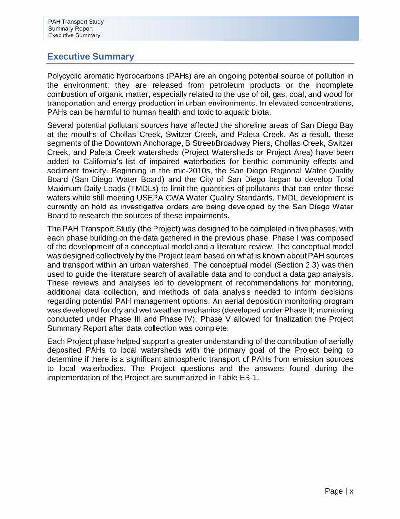
Polycyclic aromatic hydrocarbons (PAHs) are an ongoing potential source of pollution in the environment; they are released from petroleum products or the incomplete combustion of organic matter, especially related to the use of oil, gas, coal, and wood for transportation and energy production in urban environments. In elevated concentrations, PAHs can be harmful to human health and toxic to aquatic biota.
Several potential pollutant sources have affected the shoreline areas of San Diego Bay at the mouths of Chollas Creek, Switzer Creek, and Paleta Creek. As a result, these segments of the Downtown Anchorage, B Street/Broadway Piers, Chollas Creek, Switzer Creek, and Paleta Creek watersheds (Project Watersheds or Project Area) have been added to California’s list of impaired waterbodies for benthic community effects and sediment toxicity. Beginning in the mid-2010s, the San Diego Regional Water Quality Board (San Diego Water Board) and the City of San Diego began to develop Total Maximum Daily Loads (TMDLs) to limit the quantities of pollutants that can enter these waters while still meeting USEPA CWA Water Quality Standards. TMDL development is currently on hold as investigative orders are being developed by the San Diego Water Board to research the sources of these impairments.
The PAH Transport Study (the Project) was designed to be completed in five phases, with each phase building on the data gathered in the previous phase. Phase I was composed of the development of a conceptual model and a literature review. The conceptual model was designed collectively by the Project team based on what is known about PAH sources and transport within an urban watershed. The conceptual model (Section 2.3) was then used to guide the literature search of available data and to conduct a data gap analysis. These reviews and analyses led to development of recommendations for monitoring, additional data collection, and methods of data analysis needed to inform decisions regarding potential PAH management options. An aerial deposition monitoring program was developed for dry and wet weather mechanics (developed under Phase II; monitoring conducted under Phase III and Phase IV). Phase V allowed for finalization the Project Summary Report after data collection was complete.
Each Project phase helped support a greater understanding of the contribution of aerially deposited PAHs to local watersheds with the primary goal of the Project being to determine if there is a significant atmospheric transport of PAHs from emission sources to local waterbodies. The Project questions and the answers found during the implementation of the Project are summarized in Table ES-1.
PAH Transport Study Summary Report Executive Summary
Page | xi
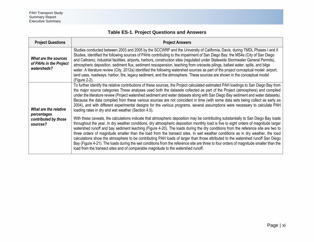
Table ES-1. Project Questions and Answers
Project Questions Project Answers
What are the sources of PAHs in the Project watersheds?
Studies conducted between 2003 and 2005 by the SCCWRP and the University of California, Davis, during TMDL Phases I and II Studies, identified the following sources of PAHs contributing to the impairment of San Diego Bay: the MS4s (City of San Diego and Caltrans), industrial facilities, airports, harbors, construction sites (regulated under Statewide Stormwater General Permits), atmospheric deposition, sediment flux, sediment resuspension, leaching from creosote pilings, ballast water, spills, and bilge water. A literature review (City, 2012a) identified the following watershed sources as part of the project conceptual model: airport, land uses, roadways, harbor, fire, legacy sediment, and the atmosphere. These sources are shown in the conceptual model (Figure 2-2).
What are the relative percentages contributed by those sources?
To further identify the relative contributions of these sources, the Project calculated estimated PAH loadings to San Diego Bay from the major source categories These analyses used both the datasets collected as part of the Project (atmosphere) and compiled under the literature review (Project watershed sediment and water datasets along with San Diego Bay sediment and water datasets). Because the data compiled from these various sources are not coincident in time (with some data sets being collect as early as 2004), and with different experimental designs for the various programs, several assumptions were necessary to calculate PAH loading rates in dry and wet weather (Section 4.5).
With these caveats, the calculations indicate that atmospheric deposition may be contributing substantially to San Diego Bay loads throughout the year. In dry weather conditions, dry atmospheric deposition monthly load is five to eight orders of magnitude larger watershed runoff and bay sediment leaching (Figure 4-20). The loads during the dry conditions from the reference site are two to three orders of magnitude smaller than the load from the transect sites. In wet weather conditions as in dry weather, the load calculations show the atmosphere to be contributing PAH loads of larger than those attributed to the watershed runoff San Diego Bay (Figure 4-21). The loads during the wet conditions from the reference site are three to four orders of magnitude smaller than the load from the transect sites and of comparable magnitude to the watershed runoff.
PAH Transport Study Summary Report Executive Summary
Table ES-1. Project Questions and Answers (continued)
Page | xii
Project Questions Project Answers
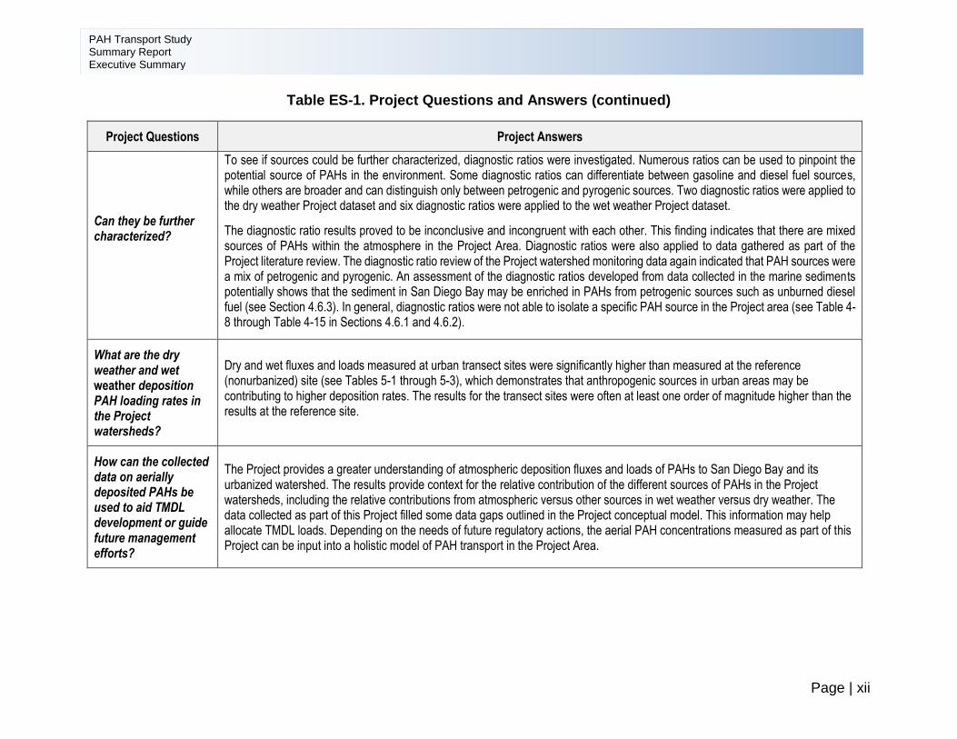
Can they be further characterized?
To see if sources could be further characterized, diagnostic ratios were investigated. Numerous ratios can be used to pinpoint the potential source of PAHs in the environment. Some diagnostic ratios can differentiate between gasoline and diesel fuel sources, while others are broader and can distinguish only between petrogenic and pyrogenic sources. Two diagnostic ratios were applied to the dry weather Project dataset and six diagnostic ratios were applied to the wet weather Project dataset.
The diagnostic ratio results proved to be inconclusive and incongruent with each other. This finding indicates that there are mixed sources of PAHs within the atmosphere in the Project Area. Diagnostic ratios were also applied to data gathered as part of the Project literature review. The diagnostic ratio review of the Project watershed monitoring data again indicated that PAH sources were a mix of petrogenic and pyrogenic. An assessment of the diagnostic ratios developed from data collected in the marine sediments potentially shows that the sediment in San Diego Bay may be enriched in PAHs from petrogenic sources such as unburned diesel fuel (see Section 4.6.3). In general, diagnostic ratios were not able to isolate a specific PAH source in the Project area (see Table 4-8 through Table 4-15 in Sections 4.6.1 and 4.6.2).
What are the dry weather and wet weather deposition PAH loading rates in the Project watersheds?
Dry and wet fluxes and loads measured at urban transect sites were significantly higher than measured at the reference (nonurbanized) site (see Tables 5-1 through 5-3), which demonstrates that anthropogenic sources in urban areas may be contributing to higher deposition rates. The results for the transect sites were often at least one order of magnitude higher than the results at the reference site.
How can the collected data on aerially deposited PAHs be used to aid TMDL development or guide future management efforts?
The Project provides a greater understanding of atmospheric deposition fluxes and loads of PAHs to San Diego Bay and its urbanized watershed. The results provide context for the relative contribution of the different sources of PAHs in the Project watersheds, including the relative contributions from atmospheric versus other sources in wet weather versus dry weather. The data collected as part of this Project filled some data gaps outlined in the Project conceptual model. This information may help allocate TMDL loads. Depending on the needs of future regulatory actions, the aerial PAH concentrations measured as part of this Project can be input into a holistic model of PAH transport in the Project Area.

PAH Transport Study Summary Report Executive Summary
Table ES-1. Project Questions and Answers (continued)
Page | xiii
Project Questions Project Answers
What are the next steps required to characterize aerial PAH sources for TMDL implementation?
What type of environmental monitoring would be needed and what would be most effective?
Data collected under this Project have addressed some data gaps. However, additional data collection or resolution in data may be advised to further the understanding of PAHs in the atmosphere and their sources. Additional study options include the following:
• To better quantify the dry weather particle deposition and vapor flux, sample collection and analysis may use a modified method to analyze the gas and particle phases separately. However, because the watershed and sediment loads estimated are so much larger than dry weather atmospheric loads, this determination may not be needed.
• Concurrent wet weather deposition samples and stream water/discharge samples could be collected and analyzed to better compare PAH atmospheric deposition and watershed loading to San Diego Bay.
• Because diagnostic ratios in the Project were inconclusive, to achieve better resolution, point source monitoring stations (rather than ambient transect sites) may be installed to determine the signal from known emission sources within the Project watershed. These data could be used for fingerprinting or other source identification methods and could potentially determine the relative contributions from more specific sources.
PAH Transport Study Summary Report Section 1 – Background
Page | 1-1
1 BACKGROUND
San Diego Bay is a unique natural resource that contains contaminated sediments (particularly at the mouths of urbanized watersheds) and does not fully support benthic communities. Several potential pollutant sources have affected the shoreline areas of San Diego Bay at the mouths of Chollas Creek, Switzer Creek, and Paleta Creek. As a result, these segments of the Downtown Anchorage, B Street/Broadway Piers, Chollas Creek, Switzer Creek, and Paleta Creek watersheds (Project Watersheds or Project Area) have been added to California’s list of impaired waterbodies for benthic community effects and sediment toxicity. Currently, investigative orders are being developed by the San Diego Regional Water Quality Control Board (San Diego Water Board) to research the sources of these impairments.
Draft total maximum daily loads (TMDLs) were previously in development by the City of San Diego (City) in collaboration with the San Diego Water Board to address sediment toxicity and benthic community degradation within the Project Area (San Diego Water Board, 2013). Previous monitoring studies identified zinc, polycyclic aromatic hydrocarbons (total PAHs), polychlorinated biphenyls (total PCBs), and Chlordane as the pollutants of concern in these areas. Concentrations of these toxic pollutants threaten or impair the marine habitat (MAR) beneficial use of these waterbodies, based on the benthic community sediment quality objectives (SQOs) defined in the State Water Resources Control Board (SWRCB) Water Quality Control Plan for Enclosed Bays and Estuaries.
PCBs and Chlordane have been banned by the United States Environmental Protection Agency (USEPA) and are legacy pollutants. Numerous studies have addressed the sources of zinc in local watersheds (City, 2007; City, 2009a; City, 2009b), but the sources of PAHs, along with their fate and transport, are less understood. The City Transportation and Stormwater Department initiated the PAH Transport Study (the Project) as a special study to identify the sources of PAHs in local watersheds. The SWRCB has sponsored the final phase of the Project to collect data needed to better understand the sources of PAHs, relative contributions, and transport pathways. These data are necessary to develop more effective and defensible TMDLs or other regulatory strategies. Ultimately, the Project addresses two primary data gaps: (1) estimates of aerial deposition loading to San Diego Bay and Project watersheds; and (2) estimates of relative percent contributions from various sources.
1.1 PAHs in the Environment
PAHs are an ongoing potential source of pollution in the environment; they are released from petroleum products or the incomplete combustion of organic matter, especially related to the use of oil, gas, coal, and wood for transportation and energy production in urban environments. In elevated concentrations, PAHs can be harmful to human health and toxic to aquatic biota. Generally, the presence of PAHs in the environment has increased over the last 100 years; however, global concentrations may have stabilized because of recent air and water quality regulations (Rhea et al., 2005).
PAH Transport Study Summary Report Section 1 – Background
Page | 1-2
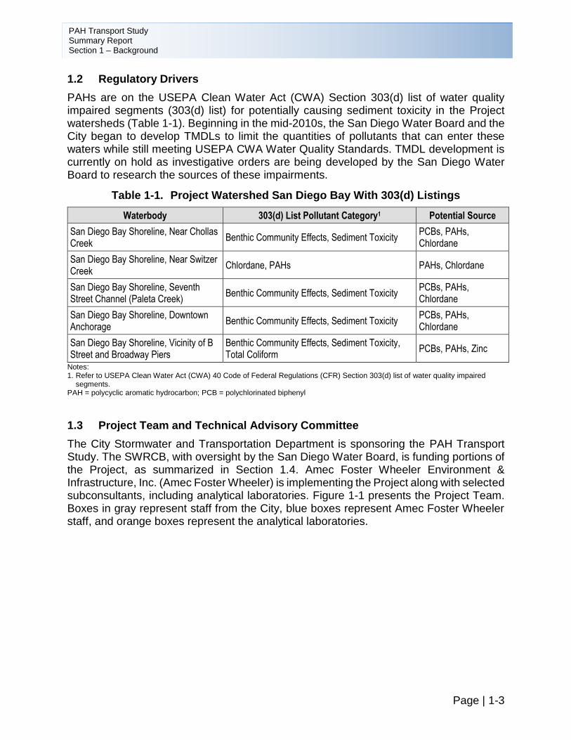
Although there are many PAHs, most regulations, analyses, and data reporting focus on only a limited number of PAHs, composed of 14 to 20 individual PAH compounds (Abdel-Shafy and Mansour, 2016).The USEPA has designated 16 PAH compounds as priority pollutants, although several researchers have suggested that the list should be updated to reflect the current state of knowledge (Andersson and Achten, 2015; Stout, 2015). These compounds are often targeted for measurement in environmental samples:
• Naphthalene
• Acenaphthylene
• Acenaphthene
• Fluorene
• Phenanthrene
• Anthracene
• Fluoranthene
• Pyrene
• Benzo(a)anthracene
• Chrysene
• Benzo(b)fluoranthene
• Benzo(k)fluoranthene
• Benzo(a)pyrene
• Dibenzo(a,h)anthracene
• Benzo(g,h,i)perylene
• Indeno(1,2,3-cd)pyrene
This Project addresses these and an additional 11 PAH compounds (discussed in Section 3).
PAHs, typically transported to and from the atmosphere into the watershed via wet and dry weather deposition, present a challenge for environmental managers because the PAHs may be from sources outside of their jurisdictions. Once released, pollutants can be carried by the wind, away from their sources, to other places via the atmosphere (Lavin et al., 2011). Atmospheric deposition can be a significant source of PAHs to the surface waters of lakes, estuaries, and the remote ocean, especially waters downwind of urban and industrialized areas (Park et al., 2001). PAHs may undergo adsorption, volatilization, photolysis, and chemical degradation. Microbial degradation is identified as the major degradation process, and is being researched as a potential remediation tool (Abdel-Shafy and Mansour, 2016).
In southern California, emissions of semi-volatile organic compounds including PAHs into the atmosphere and subsequent deposition account for a significant portion of PAH loading to waterbodies (Sabin et al., 2004). Determining the sources and relative contributions of atmospheric deposition of PAHs is challenging. Because differences in the physical and chemical properties of individual PAHs affect their distribution in the environment, this information can be exploited to identify sources and determine the relative contributions of these contaminants from local and remote sources.
PAH Transport Study Summary Report Section 1 – Background
Page | 1-3
1.2 Regulatory Drivers
PAHs are on the USEPA Clean Water Act (CWA) Section 303(d) list of water quality impaired segments (303(d) list) for potentially causing sediment toxicity in the Project watersheds (Table 1-1). Beginning in the mid-2010s, the San Diego Water Board and the City began to develop TMDLs to limit the quantities of pollutants that can enter these waters while still meeting USEPA CWA Water Quality Standards. TMDL development is currently on hold as investigative orders are being developed by the San Diego Water Board to research the sources of these impairments.
Table 1-1. Project Watershed San Diego Bay With 303(d) Listings
Waterbody 303(d) List Pollutant Category1 Potential Source
San Diego Bay Shoreline, Near Chollas Creek
Benthic Community Effects, Sediment Toxicity PCBs, PAHs, Chlordane
San Diego Bay Shoreline, Near Switzer Creek
Chlordane, PAHs PAHs, Chlordane
San Diego Bay Shoreline, Seventh Street Channel (Paleta Creek)
Benthic Community Effects, Sediment Toxicity PCBs, PAHs, Chlordane
San Diego Bay Shoreline, Downtown Anchorage
Benthic Community Effects, Sediment Toxicity PCBs, PAHs, Chlordane
San Diego Bay Shoreline, Vicinity of B Street and Broadway Piers
Benthic Community Effects, Sediment Toxicity, Total Coliform
PCBs, PAHs, Zinc
Notes: 1. Refer to USEPA Clean Water Act (CWA) 40 Code of Federal Regulations (CFR) Section 303(d) list of water quality impaired
segments. PAH = polycyclic aromatic hydrocarbon; PCB = polychlorinated biphenyl
1.3 Project Team and Technical Advisory Committee
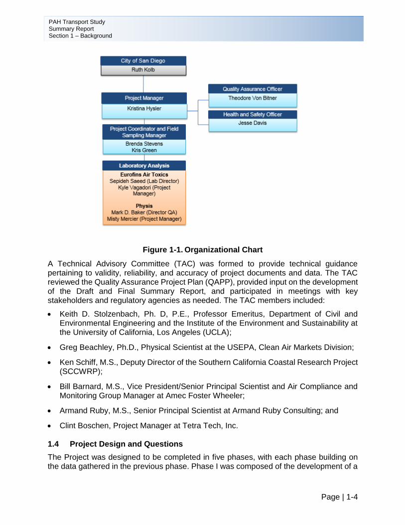
The City Stormwater and Transportation Department is sponsoring the PAH Transport Study. The SWRCB, with oversight by the San Diego Water Board, is funding portions of the Project, as summarized in Section 1.4. Amec Foster Wheeler Environment & Infrastructure, Inc. (Amec Foster Wheeler) is implementing the Project along with selected subconsultants, including analytical laboratories. Figure 1-1 presents the Project Team. Boxes in gray represent staff from the City, blue boxes represent Amec Foster Wheeler staff, and orange boxes represent the analytical laboratories.
PAH Transport Study Summary Report Section 1 – Background
Page | 1-4
Figure 1-1. Organizational Chart
A Technical Advisory Committee (TAC) was formed to provide technical guidance pertaining to validity, reliability, and accuracy of project documents and data. The TAC reviewed the Quality Assurance Project Plan (QAPP), provided input on the development of the Draft and Final Summary Report, and participated in meetings with key stakeholders and regulatory agencies as needed. The TAC members included:
• Keith D. Stolzenbach, Ph. D, P.E., Professor Emeritus, Department of Civil and Environmental Engineering and the Institute of the Environment and Sustainability at the University of California, Los Angeles (UCLA);
• Greg Beachley, Ph.D., Physical Scientist at the USEPA, Clean Air Markets Division;
• Ken Schiff, M.S., Deputy Director of the Southern California Coastal Research Project (SCCWRP);
• Bill Barnard, M.S., Vice President/Senior Principal Scientist and Air Compliance and Monitoring Group Manager at Amec Foster Wheeler;
• Armand Ruby, M.S., Senior Principal Scientist at Armand Ruby Consulting; and
• Clint Boschen, Project Manager at Tetra Tech, Inc.
1.4 Project Design and Questions
The Project was designed to be completed in five phases, with each phase building on the data gathered in the previous phase. Phase I was composed of the development of a
PAH Transport Study Summary Report Section 1 – Background
Page | 1-5
conceptual model and a literature review. The conceptual model was designed collectively by the Project team based on what is known about PAH sources and transport within an urban watershed. The conceptual model (Section 2.3) was then used to guide the literature search of available data and to conduct a data gap analysis. The literature search involved a broad review of documents regarding current data and research into sources, transport, and prevalence of PAHs as they relate to the Project watersheds and Project questions. A total of 29 literature sources were reviewed. They identified potential sources within the watershed, suggested monitoring methodologies, and outlined methods for source identification and allocation (City, 2012a). Objectives, scopes, and findings from the literature review for each potential source included in the conceptual model (airport, land uses, roadways, harbor, fire, legacy sediment, and atmosphere) were summarized in the PAH Transport Study Development Technical Memorandum (City, 2012b).
Available data including atmospheric concentration data, dry and wet weather runoff data, and sediment quality data collected throughout the Project watersheds were evaluated to identify data gaps. Water and sediment quality data have been collected in the Project watersheds by the City and by other entities, including by SCCWRP. It was determined that adequate water and sediment quality data representative of various portions of the Project watersheds or subwatersheds have been collected to characterize PAH concentrations within San Diego Bay and the municipal separate storm sewer systems (MS4s) and creeks. However, it was determined that data on atmospheric concentrations and deposition of PAHs may be limited. In southern California, the lack of atmospheric data may be because current air quality monitoring programs such as the Clean Air Status and Trends Network (CASTNET), the National Atmospheric Deposition Program (NADP), the USEPA Clean Air Markets Data and Maps, and the USEPA Toxic Release Inventory (TRI) did not provide data with fine-enough resolution, or were focused on impacts relative to human health rather than ecological health (City, 2012b). Based on the data gap analysis, an aerial deposition monitoring program was developed for dry and wet weather mechanics (developed under Phase II; monitoring conducted under Phase III and Phase IV). Phase V allowed for finalization the Project Summary Report after data collection was complete.
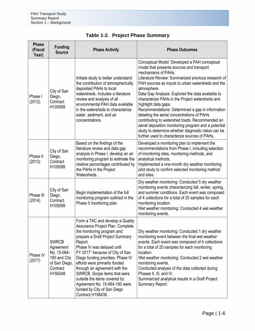
The phases mirror the City’s fiscal calendar year (July 1 through June 30). Each fiscal year (FY) is named for the year in which it ends. For example, FY 2012 runs from July 1, 2011, through June 30, 2012. Work began in FY 2012 and continued into FY 2017. Phases I, II, and III were funded by the City Transportation and Stormwater Department. The Project was put on hold after FY 2014 because of other funding priorities for the City. The San Diego Water Board was interested in continuing the Project to inform regional regulatory activities and requested a scope and budget from the City for the remaining phases. A proposal was submitted to the SWRCB and was accepted for state support. Phases IV and V were sponsored by the SWRCB under Agreement Number 15-064-190. Table 1-2 summarizes the Project phases and describes activities performed under each phase.
PAH Transport Study Summary Report Section 1 – Background
Page | 1-6
Table 1-2. Project Phase Summary
Phase (Fiscal Year)
Funding Source
Phase Activity Phase Outcomes
Phase I (2012)
City of San Diego, Contract H105099
Initiate study to better understand the contribution of atmospherically deposited PAHs to local watersheds. Includes a literature review and analysis of all environmental PAH data available in the watersheds to characterize water, sediment, and air concentrations.
Conceptual Model: Developed a PAH conceptual model that presents sources and transport mechanisms of PAHs. Literature Review: Summarized previous research of PAH sources as inputs to urban watersheds and the atmosphere. Data Gap Analysis: Explored the data available to characterize PAHs in the Project watersheds and highlight data gaps. Recommendations: Determined a gap in information detailing the aerial concentrations of PAHs contributing to watershed loads. Recommended an aerial deposition monitoring program and a potential study to determine whether diagnostic ratios can be further used to characterize sources of PAHs.
Phase II (2013)
City of San Diego, Contract H105099
Based on the findings of the literature review and data gap analysis in Phase I, develop an air monitoring program to estimate the relative percentages contributed by the PAHs in the Project Watersheds.
Developed a monitoring plan to implement the recommendations from Phase I, including selection of monitoring sites, monitoring methods, and analytical methods. Implemented a one-month dry weather monitoring pilot study to confirm selected monitoring method and sites.
Phase III (2014)
City of San Diego, Contract H105099
Begin implementation of the full monitoring program outlined in the Phase II monitoring plan.
Dry weather monitoring: Conducted 5 dry weather monitoring events characterizing fall, winter, spring, and summer conditions. Each event was composed of 4 collections for a total of 20 samples for each monitoring location. Wet weather monitoring: Conducted 4 wet weather monitoring events.
Phase IV (2017)
SWRCB Agreement No. 15-064-190 and City of San Diego, Contract H156348
Form a TAC and develop a Quality Assurance Project Plan. Complete the monitoring program and prepare a Draft Project Summary Report. Phase IV was delayed until FY 20171 because of City of San Diego funding priorities. Phase IV efforts were primarily funded through an agreement with the SWRCB. Scope items that were outside the items covered by Agreement No. 15-064-190 were funded by City of San Diego Contract H156438.
Dry weather monitoring: Conducted 1 dry weather monitoring event between the final wet weather events. Each event was composed of 4 collections for a total of 20 samples for each monitoring location. Wet weather monitoring: Conducted 2 wet weather monitoring events. Conducted analysis of the data collected during Phases II, III, and IV. Summarized analytical results in a Draft Project Summary Report.
PAH Transport Study Summary Report Section 1 – Background
Table 1-2. Project Phase Summary (continued)
Page | 1-7
Phase (Fiscal Year)
Funding Source
Phase Activity Phase Outcomes
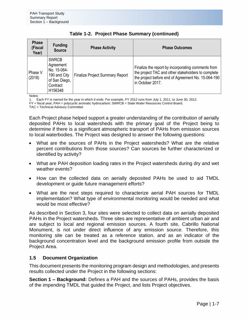
Phase V (2018)
SWRCB Agreement No. 15-064-190 and City of San Diego, Contract H156348
Finalize Project Summary Report
Finalize the report by incorporating comments from the project TAC and other stakeholders to complete the project before end of Agreement No. 15-064-190 in October 2017.
Notes: 1. Each FY is named for the year in which it ends. For example, FY 2012 runs from July 1, 2011, to June 30, 2012. FY = fiscal year; PAH = polycyclic aromatic hydrocarbon; SWRCB = State Water Resources Control Board; TAC = Technical Advisory Committee
Each Project phase helped support a greater understanding of the contribution of aerially deposited PAHs to local watersheds with the primary goal of the Project being to determine if there is a significant atmospheric transport of PAHs from emission sources to local waterbodies. The Project was designed to answer the following questions:
• What are the sources of PAHs in the Project watersheds? What are the relative percent contributions from those sources? Can sources be further characterized or identified by activity?
• What are PAH deposition loading rates in the Project watersheds during dry and wet weather events?
• How can the collected data on aerially deposited PAHs be used to aid TMDL development or guide future management efforts?
• What are the next steps required to characterize aerial PAH sources for TMDL implementation? What type of environmental monitoring would be needed and what would be most effective?
As described in Section 3, four sites were selected to collect data on aerially deposited PAHs in the Project watersheds. Three sites are representative of ambient urban air and are subject to local and regional emission sources. A fourth site, Cabrillo National Monument, is not under direct influence of any emission source. Therefore, this monitoring site can be treated as a reference station, and as an indicator of the background concentration level and the background emission profile from outside the Project Area.
1.5 Document Organization
This document presents the monitoring program design and methodologies, and presents results collected under the Project in the following sections:
Section 1 – Background: Defines a PAH and the sources of PAHs, provides the basis of the impending TMDL that guided the Project, and lists Project objectives.
PAH Transport Study Summary Report Section 1 – Background
Page | 1-8
Section 2 – PAH Sources and Transport Mechanisms: Discusses transport mechanisms of PAHs, and presents the conceptual model.
Section 3 – Atmospheric Deposition Monitoring Technical Approach: Presents details on site selection, monitoring techniques, and analytical methodologies for dry and wet weather deposition monitoring.
Section 4 – Results: Summarizes the results of the data analyses, including summary statistics and application of diagnostic ratios for source identification and allocation.
Section 5 – Conclusions and Recommendations: Provides an overall summary of conclusions of the Project as well as recommendations for next steps.
Section 6 – References: Provides citations for references used to develop this document.
PAH Transport Study Summary Report Section 2 – Review of PAH Sources and Transport Mechanisms
Page | 2-1
2 REVIEW OF PAH SOURCES AND TRANSPORT MECHANISMS
The atmosphere of the Project watersheds is subject to various inputs of PAHs produced by both stationary and mobile sources of incomplete combustion with emissions from anthropogenic activities predominating. Nevertheless, some PAHs may originate from natural sources such as open burning, natural losses or seepage of petroleum or coal deposits, and volcanic activities. PAHs from different sources have different chemical characteristics. For example, PAHs can be found in both the gaseous-phase or sorbed to aerosols (particulate phase) in ambient air. Atmospheric partitioning of PAH compounds between the particulate and the gaseous phases strongly influences their fate and transport in the atmosphere. This section summarizes the characteristics of different PAH compounds, their transport mechanisms, and deposition processes. Based on knowledge of Project watershed PAH sources and their known behavior in the environment, the Project conceptual model was developed.
2.1 Characteristics of PAHs
Chemically, PAHs are defined as compounds consisting of only carbon and hydrogen atoms. They are semi-volatile organic compounds consisting two to seven benzene rings bonded in linear, cluster, or angular arrangements.
PAHs have two primary origins: a pyrogenic origin if they are derived from incomplete combustion (petroleum and other organic materials), or petrogenic if they are derived from non-combusted petroleum-based materials (typically associated with transportation, storage, and use of crude oil and crude oil products, including oceanic and freshwater oil spills, underground and above ground storage tank leaks, small releases of gasoline, motor oil, and related substances associated with transportation, asphalt, or various refinery products). Wood-burning fireplaces in homes can also be persistent sources of small amounts of PAHs (Tobiszewski and Namieśnik, 2012). In urbanized areas, most PAHs in the environment are from both pyrogenic and petrogenic anthropogenic sources (Maliszewska-Kordybach, 1999; Tran et al., 1996). PAHs released from natural sources such as wildfires and volcanic activity, can cause high amounts of deposition during short-lived, large events. PAHs may also be released biologically, through synthesis by certain plants and bacteria or formed during the degradation of vegetative matter (Abdel-Shafy and Mansour, 2016).
PAHs are commonly classified into two groups based on their molecular structure. Differences in the structure and size of individual PAHs result in substantial variability in the physical and chemical properties of these compounds. PAHs are generally hydrophobic organic chemicals with low vapor pressures, although these characteristics decrease with increasing molecular weight. Low molecular weight (LMW) compounds contain three or fewer benzene rings and tend to be more water soluble, are less lipophilic, and have higher vapor pressures; therefore, they tend to be associated with the vapor phase. LMW PAH compounds are generally produced through low-temperature processes (Maliszewska-Kordybach, 1999). High molecular weight (HMW) PAH compounds contain four or more benzene rings and tend to be less water soluble, are more lipophilic, and have lower vapor pressures, making them more likely to be found
PAH Transport Study Summary Report Section 2 – Review of PAH Sources and Transport Mechanisms
Page | 2-2
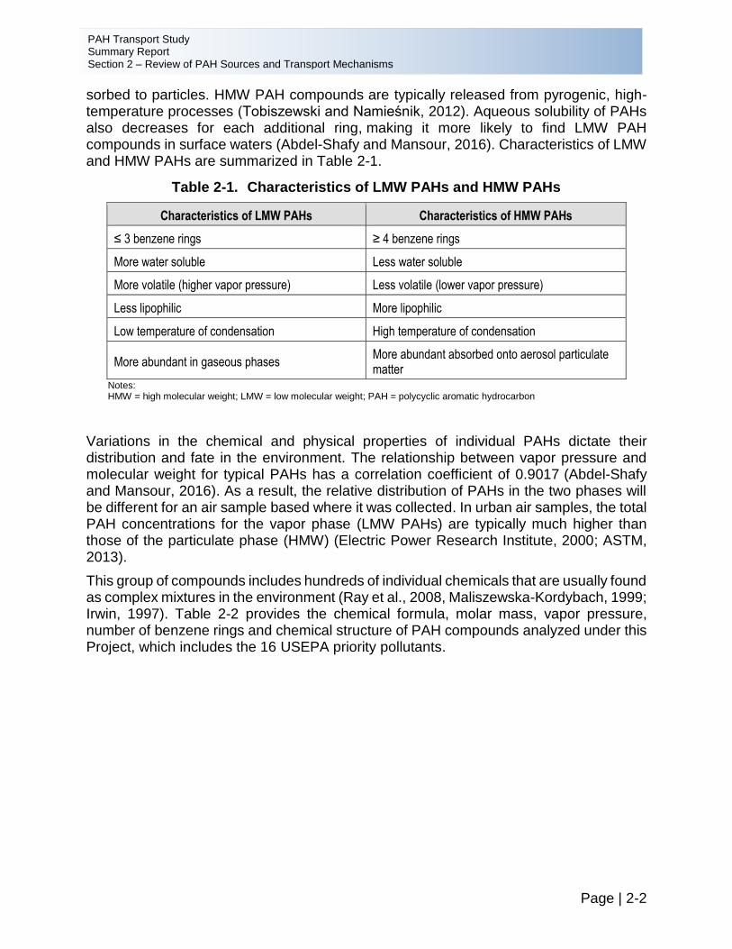
sorbed to particles. HMW PAH compounds are typically released from pyrogenic, high-temperature processes (Tobiszewski and Namieśnik, 2012). Aqueous solubility of PAHs also decreases for each additional ring, making it more likely to find LMW PAH compounds in surface waters (Abdel-Shafy and Mansour, 2016). Characteristics of LMW and HMW PAHs are summarized in Table 2-1.
Table 2-1. Characteristics of LMW PAHs and HMW PAHs
Characteristics of LMW PAHs Characteristics of HMW PAHs
≤ 3 benzene rings ≥ 4 benzene rings
More water soluble Less water soluble
More volatile (higher vapor pressure) Less volatile (lower vapor pressure)
Less lipophilic More lipophilic
Low temperature of condensation High temperature of condensation
More abundant in gaseous phases More abundant absorbed onto aerosol particulate matter
Notes: HMW = high molecular weight; LMW = low molecular weight; PAH = polycyclic aromatic hydrocarbon
Variations in the chemical and physical properties of individual PAHs dictate their distribution and fate in the environment. The relationship between vapor pressure and molecular weight for typical PAHs has a correlation coefficient of 0.9017 (Abdel-Shafy and Mansour, 2016). As a result, the relative distribution of PAHs in the two phases will be different for an air sample based where it was collected. In urban air samples, the total PAH concentrations for the vapor phase (LMW PAHs) are typically much higher than those of the particulate phase (HMW) (Electric Power Research Institute, 2000; ASTM, 2013).
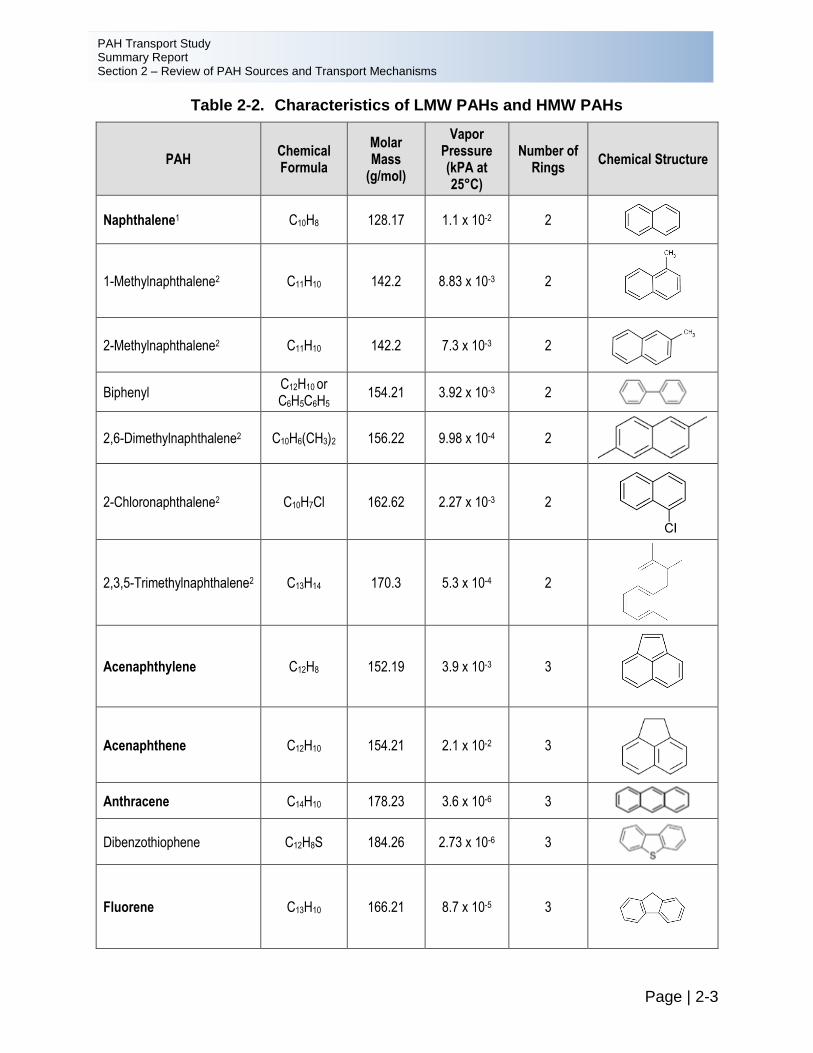
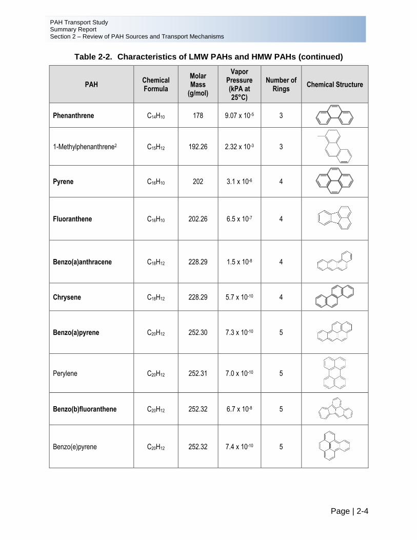
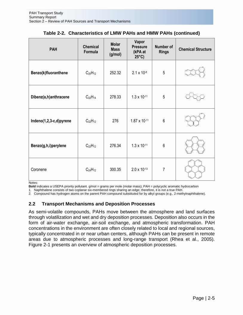
This group of compounds includes hundreds of individual chemicals that are usually found as complex mixtures in the environment (Ray et al., 2008, Maliszewska-Kordybach, 1999; Irwin, 1997). Table 2-2 provides the chemical formula, molar mass, vapor pressure, number of benzene rings and chemical structure of PAH compounds analyzed under this Project, which includes the 16 USEPA priority pollutants.
PAH Transport Study Summary Report Section 2 – Review of PAH Sources and Transport Mechanisms
Page | 2-3
Table 2-2. Characteristics of LMW PAHs and HMW PAHs
PAH Chemical Formula
Molar Mass
(g/mol)
Vapor Pressure (kPA at 25°C)
Number of Rings
Chemical Structure
Naphthalene1 C10H8 128.17 1.1 x 10⁻² 2
1-Methylnaphthalene2 C11H10 142.2 8.83 x 10⁻³ 2
2-Methylnaphthalene2 C11H10 142.2 7.3 x 10⁻³ 2
Biphenyl C12H10 or C6H5C6H5
154.21 3.92 x 10⁻³ 2
2,6-Dimethylnaphthalene2 C10H6(CH3)2 156.22 9.98 x 10⁻⁴ 2
2-Chloronaphthalene2 C10H7Cl 162.62 2.27 x 10⁻³ 2
2,3,5-Trimethylnaphthalene2 C13H14 170.3 5.3 x 10⁻⁴ 2
Acenaphthylene C12H8 152.19 3.9 x 10⁻³ 3
Acenaphthene C12H10 154.21 2.1 x 10⁻² 3
Anthracene C14H10 178.23 3.6 x 10⁻⁶ 3
Dibenzothiophene C12H8S 184.26 2.73 x 10⁻⁶ 3
Fluorene C13H10 166.21 8.7 x 10⁻⁵ 3
PAH Transport Study Summary Report Section 2 – Review of PAH Sources and Transport Mechanisms
Table 2-2. Characteristics of LMW PAHs and HMW PAHs (continued)
Page | 2-4
PAH Chemical Formula
Molar Mass
(g/mol)
Vapor Pressure (kPA at 25°C)
Number of Rings
Chemical Structure
Phenanthrene C14H10 178 9.07 x 10⁻⁵ 3
1-Methylphenanthrene2 C15H12 192.26 2.32 x 10⁻³ 3
Pyrene C16H10 202 3.1 x 10⁻⁶ 4
Fluoranthene C16H10 202.26 6.5 x 10⁻⁷ 4
Benzo(a)anthracene C18H12 228.29 1.5 x 10⁻⁸ 4
Chrysene C18H12 228.29 5.7 x 10⁻¹⁰ 4
Benzo(a)pyrene C20H12 252.30 7.3 x 10⁻¹⁰ 5
Perylene C20H12 252.31 7.0 x 10⁻¹⁰ 5
Benzo(b)fluoranthene C20H12 252.32 6.7 x 10⁻⁸ 5
Benzo(e)pyrene C20H12 252.32 7.4 x 10⁻¹⁰ 5
PAH Transport Study Summary Report Section 2 – Review of PAH Sources and Transport Mechanisms
Table 2-2. Characteristics of LMW PAHs and HMW PAHs (continued)
Page | 2-5
PAH Chemical Formula
Molar Mass
(g/mol)
Vapor Pressure (kPA at 25°C)
Number of Rings
Chemical Structure
Benzo(k)fluoranthene C20H12 252.32 2.1 x 10⁻⁸ 5
Dibenz(a,h)anthracene C22H14 278.33 1.3 x 10⁻¹¹ 5
Indeno(1,2,3-c,d)pyrene C22H12 276 1.87 x 10⁻¹¹ 6
Benzo(g,h,i)perylene C22H12 276.34 1.3 x 10⁻¹¹ 6
Coronene C24H12 300.35 2.0 x 10⁻¹³ 7
Notes: Bold indicates a USEPA priority pollutant. g/mol = grams per mole (molar mass); PAH = polycyclic aromatic hydrocarbon 1. Naphthalene consists of two coplanar six-membered rings sharing an edge; therefore, it is not a true PAH. 2. Compound has hydrogen atoms on the parent PAH compound substituted for by alkyl groups (e.g., 2-methylnaphthalene).
2.2 Transport Mechanisms and Deposition Processes
As semi-volatile compounds, PAHs move between the atmosphere and land surfaces through volatilization and wet and dry deposition processes. Deposition also occurs in the form of air-water exchange, air-soil exchange, and atmospheric transformation. PAH concentrations in the environment are often closely related to local and regional sources, typically concentrated in or near urban centers, although PAHs can be present in remote areas due to atmospheric processes and long-range transport (Rhea et al., 2005). Figure 2-1 presents an overview of atmospheric deposition processes.
PAH Transport Study Summary Report Section 2 – Review of PAH Sources and Transport Mechanisms
Page | 2-6
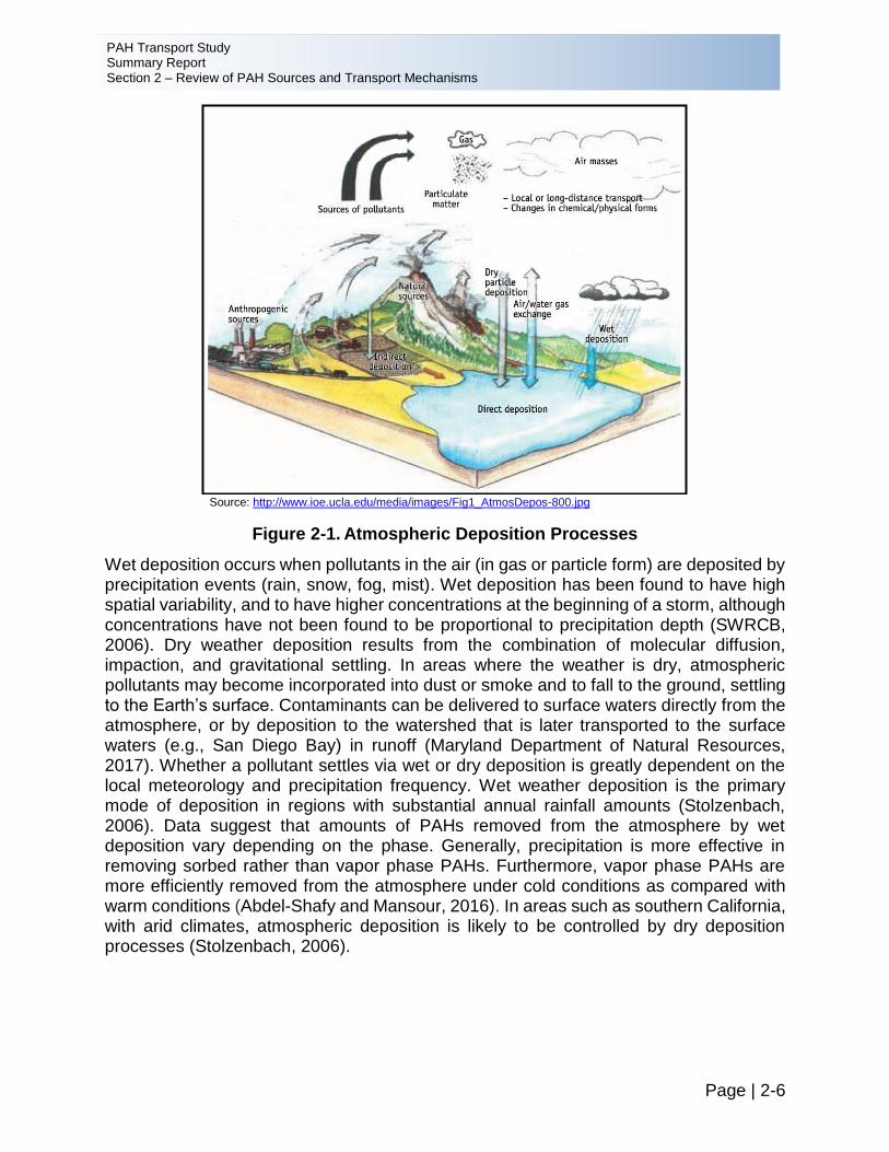
Source: http://www.ioe.ucla.edu/media/images/Fig1_AtmosDepos-800.jpg
Figure 2-1. Atmospheric Deposition Processes
Wet deposition occurs when pollutants in the air (in gas or particle form) are deposited by precipitation events (rain, snow, fog, mist). Wet deposition has been found to have high spatial variability, and to have higher concentrations at the beginning of a storm, although concentrations have not been found to be proportional to precipitation depth (SWRCB, 2006). Dry weather deposition results from the combination of molecular diffusion, impaction, and gravitational settling. In areas where the weather is dry, atmospheric pollutants may become incorporated into dust or smoke and to fall to the ground, settling to the Earth’s surface. Contaminants can be delivered to surface waters directly from the atmosphere, or by deposition to the watershed that is later transported to the surface waters (e.g., San Diego Bay) in runoff (Maryland Department of Natural Resources, 2017). Whether a pollutant settles via wet or dry deposition is greatly dependent on the local meteorology and precipitation frequency. Wet weather deposition is the primary mode of deposition in regions with substantial annual rainfall amounts (Stolzenbach, 2006). Data suggest that amounts of PAHs removed from the atmosphere by wet deposition vary depending on the phase. Generally, precipitation is more effective in removing sorbed rather than vapor phase PAHs. Furthermore, vapor phase PAHs are more efficiently removed from the atmosphere under cold conditions as compared with warm conditions (Abdel-Shafy and Mansour, 2016). In areas such as southern California, with arid climates, atmospheric deposition is likely to be controlled by dry deposition processes (Stolzenbach, 2006).
PAH Transport Study Summary Report Section 2 – Review of PAH Sources and Transport Mechanisms
Page | 2-7
2.3 PAH Transport and Source Conceptual Model Diagram
PAHs are released into the environment each year from a variety of natural (e.g., forest fires and volcanic explosions) and anthropogenic (e.g., industrial activities, fossil fuel combustion, and transportation and energy production) sources.
Studies conducted between 2003 and 2005 by SCCWRP and the University of California, Davis, during TMDL Phases I and II Studies, identified the following sources of PAHs contributing to the impairment of San Diego Bay:
• MS4s (City and California Department of Transportation [Caltrans]);
• Industrial facilities, including airports and harbors (regulated under Statewide Stormwater General Permits);
• Construction sites (regulated under Statewide Stormwater General Permits); and
• Others, including atmospheric deposition, sediment flux, sediment resuspension, leaching from creosote pilings, ballast water, spills, and bilge water.
Additional military activities, or facilities regulated under other stormwater or individual source permits, may exist but were not included in the original study design. To begin to address the Project questions (Section 1.4), the Project team collectively designed a conceptual model based on what is known about PAH sources and transport within an urban watershed. The conceptual model was then used to guide the literature search of available data and to conduct a data gap analysis. These reviews and analyses led to development of recommendations for monitoring, additional data collection, and methods of data analysis needed to inform decisions regarding potential PAH management options.
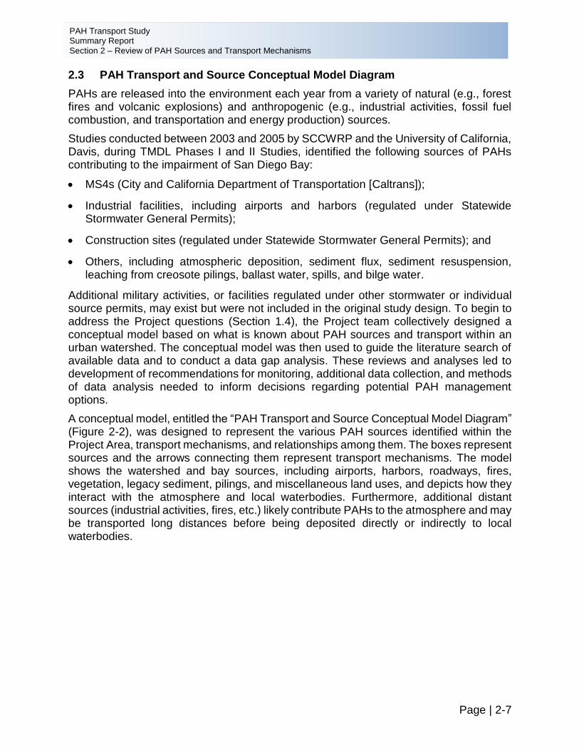
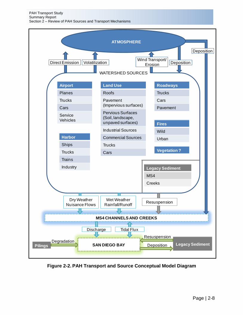
A conceptual model, entitled the “PAH Transport and Source Conceptual Model Diagram” (Figure 2-2), was designed to represent the various PAH sources identified within the Project Area, transport mechanisms, and relationships among them. The boxes represent sources and the arrows connecting them represent transport mechanisms. The model shows the watershed and bay sources, including airports, harbors, roadways, fires, vegetation, legacy sediment, pilings, and miscellaneous land uses, and depicts how they interact with the atmosphere and local waterbodies. Furthermore, additional distant sources (industrial activities, fires, etc.) likely contribute PAHs to the atmosphere and may be transported long distances before being deposited directly or indirectly to local waterbodies.
PAH Transport Study Summary Report Section 2 – Review of PAH Sources and Transport Mechanisms
Page | 2-8
Figure 2-2. PAH Transport and Source Conceptual Model Diagram
Airport
Planes
Trucks
Cars
Service
Vehicles
Land Use
Roofs
Pavement
(Impervious surfaces)
Pervious Surfaces
(Soil, landscape,
unpaved surfaces)
Industrial Sources
Commercial Sources
Trucks
Cars
Harbor
Ships
Trucks
Trains
Industry
Roadways
Trucks
Cars
Pavement
Fires
Wild
Urban
Vegetation ?
Volatilization
WATERSHED SOURCES
Wind Transport/
ErosionDirect Emission Deposition
MS4 CHANNELS AND CREEKS
SAN DIEGO BAY
ResuspensionDry Weather
Nuisance Flows
Wet Weather
Rainfall/Runoff
ATMOSPHERE
Resuspension
PilingsDegradation
Legacy Sediment
Deposition
Tidal FluxDischarge
Deposition
Legacy Sediment
MS4
Creeks
PAH Transport Study Summary Report Section 3 – Atmospheric Deposition Monitoring Technical Approach
Page | 3-1
3 ATMOSPHERIC DEPOSITION MONITORING TECHNICAL
APPROACH
Based on the Phase I data gap analysis, an aerial deposition monitoring program was developed (Phase II). The mechanics of PAH aerial transport vary under different weather conditions. Therefore, the atmospheric deposition monitoring program consisted of both dry weather (air) and wet weather (water) deposition monitoring components. Monitoring program design and methodologies, equipment selection and installation, and analytical methods are described in this section.
In developing the aerial deposition monitoring plan, the Project team considered nationally available documents such as the NADP Installation Manual (NADP, 2011) and USEPA Methods TO-13 and TO-13A and included the following:
• Site selection;
• Monitoring protocol and equipment selection for dry and wet weather program components, including meteorological parameter monitoring; and
• Analytical laboratory selection.
Measuring dry weather deposition of PAHs specifically is difficult because dry weather deposition rates and mechanisms vary between the particle and gaseous phases (Lee and Nicholson, 1994). No standard technique exists for direct measurement of the dry weather deposition of PAHs. Available monitoring techniques include collecting dry particles and gases on a depositional surface or measuring the amount of dry particles and gases in the air with a high-volume air sampler (ambient air monitoring) and calculating a deposition rate. According to the USEPA, ambient air monitoring methods are considered to be more accurate (USEPA, 2001); this method was used for this Project for dry depositional monitoring.
The wet weather deposition monitoring methodology was guided by the NADP, which has monitored precipitation (rainfall) chemistry for many years. Wet weather deposition monitoring was conducted using an automated atmospheric deposition sampler.
Monitoring methods are documented in detail in the Project QAPP (City, 2016) and monitoring plan (City, 2013) provided in Appendix A. Methodologies are summarized in the Sections 3.1 through 3.4.
3.1 Site Selection and Descriptions
Site selection and equipment installation was performed following guidelines in the NADP Installation Manual (NADP, 2011). The Project team selected sites after completing a desktop geographic information system (GIS) survey and field investigation that focused on City-owned properties. These properties were selected along a transect following the prevailing wind pattern direction to determine the most representative sites of ambient air in the Project watersheds. Based on hourly data collected over 10 years (from 1992 to 2002), the prevailing winds in San Diego originate from the west-northwest (WNW) (Desert Research Institute [DRI], 2012; National Weather Service [NWS], 2012).
PAH Transport Study Summary Report Section 3 – Atmospheric Deposition Monitoring Technical Approach
Page | 3-2
Atmospheric conditions and topography affect the spatial and temporal variability of PAH concentrations, transport, and deposition (USEPA, 2008) and must be considered during site selection. Atmospheric conditions include wind speed, wind direction, and humidity. Wind direction controls the direction of transport, and wind speed controls travel time and dilution rates of pollutants in the air by controlling turbulent diffusion. Atmospheric turbulence can also be increased by mechanical (caused by structures and changes in terrain) or thermal features (caused by differential heating and cooling of land and water surfaces). Surrounding buildings, vegetation, and land surfaces affect air trajectories, which can produce local anomalies in pollutant concentrations because of changes in transport and diffusion of pollutant-laden air. Major topographical features were avoided in monitoring site selection, but several small canyons with approximately 300 feet of relief are found in the Project Area near the urban monitoring sites, and the reference site is located on the leeward side of an approximately 400-foot coastal ridge.
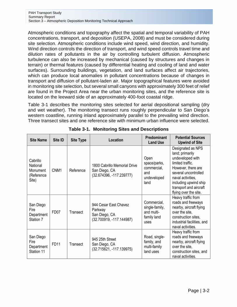
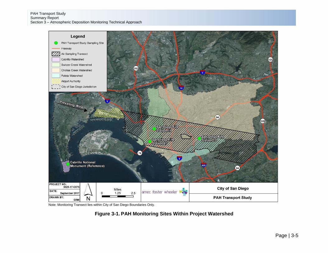
Table 3-1 describes the monitoring sites selected for aerial depositional sampling (dry and wet weather). The monitoring transect runs roughly perpendicular to San Diego’s western coastline, running inland approximately parallel to the prevailing wind direction. Three transect sites and one reference site with minimum urban influence were selected.
Table 3-1. Monitoring Sites and Descriptions
Site Name Site ID Site Type Location Predominant
Land Use Potential Sources
Upwind of Site
Cabrillo National Monument (Reference Site)
CNM1 Reference 1800 Cabrillo Memorial Drive San Diego, CA (32.674396, -117.239777)
Open space/parks, commercial, and undeveloped land
Designated as NPS land; primarily undeveloped with limited traffic. However, there are several uncontrolled naval activities, including upwind ship transport and aircraft flying over the site.
San Diego Fire Department Station 7
FD07 Transect
944 Cesar East Chavez Parkway San Diego, CA (32.700919, -117.144987)
Commercial, single-family, and multi-family land uses
Heavy traffic from roads and freeways nearby, aircraft flying over the site, construction sites, industrial facilities, and naval activities.
San Diego Fire Department Station 11
FD11 Transect 945 25th Street San Diego, CA (32.715621, -117.139975)
Road, single-family, and multi-family land uses
Heavy traffic from roads and freeways nearby, aircraft flying over the site, construction sites, and naval activities.
PAH Transport Study Summary Report Section 3 – Atmospheric Deposition Monitoring Technical Approach
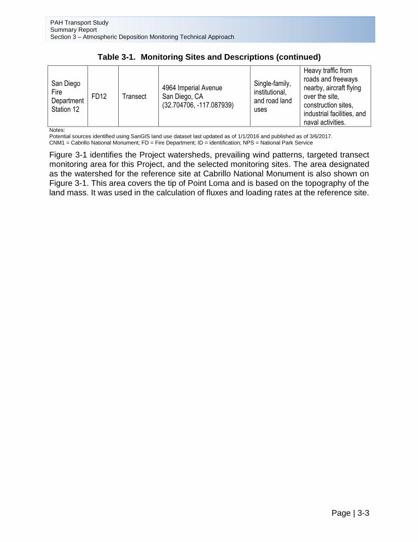
Table 3-1. Monitoring Sites and Descriptions (continued)
Page | 3-3
San Diego Fire Department Station 12
FD12 Transect 4964 Imperial Avenue San Diego, CA (32.704706, -117.087939)
Single-family, institutional, and road land uses
Heavy traffic from roads and freeways nearby, aircraft flying over the site, construction sites, industrial facilities, and naval activities.
Notes: Potential sources identified using SanGIS land use dataset last updated as of 1/1/2016 and published as of 3/6/2017. CNM1 = Cabrillo National Monument; FD = Fire Department; ID = identification; NPS = National Park Service
Figure 3-1 identifies the Project watersheds, prevailing wind patterns, targeted transect monitoring area for this Project, and the selected monitoring sites. The area designated as the watershed for the reference site at Cabrillo National Monument is also shown on Figure 3-1. This area covers the tip of Point Loma and is based on the topography of the land mass. It was used in the calculation of fluxes and loading rates at the reference site.
PAH Transport Study Summary Report Section 3 – Atmospheric Deposition Monitoring Technical Approach
Page | 3-4
Intentionally Left Blank
PAH Transport Study Summary Report Section 3 – Atmospheric Deposition Monitoring Technical Approach
Page | 3-5
Note: Monitoring Transect lies within City of San Diego Boundaries Only.
Figure 3-1. PAH Monitoring Sites Within Project Watershed
PAH Transport Study Summary Report Section 3 – Atmospheric Deposition Monitoring Technical Approach
Page | 3-6
Intentionally Left Blank
PAH Transport Study Summary Report Section 3 – Atmospheric Deposition Monitoring Technical Approach
Page | 3-7
3.2 Analytical Methodologies
PAHs can be present in gas phase or bound to particles (e.g., water droplets, dust, ash, etc.). Most compounds are released in a distribution of particulate matter and gases; however, some compounds exist predominantly in one phase or another. Appropriate monitoring and analytical methods are required to avoid loss or degradation of volatile or thermally liable compounds, and must be suitable to the physical state of interest to provide representative data (USEPA, 1983). In addition to a literature review, consultations with laboratories and experts in the field were taken into account to select the appropriate dry weather and wet weather sample collection procedures and analytical methods.
Separate analytical methods were used for dry weather and wet weather deposition chemical analyses. The USEPA’s ambient air analysis method TO-13A was used for dry weather deposition analysis, and USEPA Method 625 was used for wet weather deposition analysis. Both methods include the 16 USEPA priority pollutant PAHs. However, USEPA Method 625 includes a more extensive list of constituents than those included in USEPA Method TO-13A. USEPA Method TO-13A is the closest match to USEPA Method 625 and includes the common list of PAHs that are analyzed in ambient air monitoring protocols. Additional information on each analytical method is presented in this section.
Dry weather deposition samples were collected in accordance with USEPA Method TO-13A, “Compendium of Methods for the Determination of Toxic Organic Compounds in Ambient Air: Determination of PAHs in Ambient Air Using Gas Chromatography/Mass Spectrometry (GC/MS)” (USEPA, 1999). A Tisch Environmental high-volume air sampler (HVAS) and quartz filter and a PUF/XAD-2® sorbent cartridge were used for sample collection. To quantify PAH concentrations, samples were extracted in solvent and then analyzed by GC/MS to estimate the mass of each PAH present. USEPA Method TO-13A GC/MS Selected Ion Monitoring (SIM) has a reporting limit of 0.1 microgram per liter (µg/L). Coronene and perylene were analyzed using a 1-point calibration with no laboratory control spike (LCS) or method detection limit (MDL) evaluation, since these were not available for these compounds.
Ensuring that the proper flow rate and total air volume are drawn through the sampling media is imperative to achieve data quality objectives (DQOs). If insufficient sample volume is collected, the sample must be concentrated at the laboratory for analysis. Therefore, sample volume determines the final reporting limits (i.e., increased sample volume lowers the final reporting limit) (Air Toxics, 2012). The measured result using USEPA Method TO-13A is presented as a concentration per air volume in nanograms per cubic meter (ng/m3). The concentration of each PAH is calculated using the analytical result and the total volume of air that has been drawn through each filter. Annual dry weather particle deposition rates were estimated from measurements of ambient particle PAH concentrations and a derived annual dry weather deposition velocity.
For wet weather deposition samples, water is collected directly into a sampling container. PAHs are extracted from the aqueous phase using a liquid-liquid extraction technique and then analyzed by GC/MS using USEPA Method 625.
PAH Transport Study Summary Report Section 3 – Atmospheric Deposition Monitoring Technical Approach
Page | 3-8
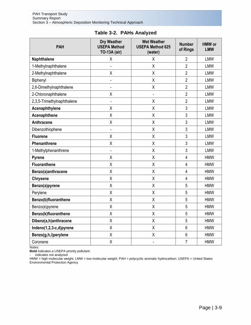
Quality assurance and quality control samples were collected in accordance with the QAPP (provided in Appendix A). Table 3-2 presents PAH compounds analyzed during dry and wet weather deposition monitoring.
Meteorological conditions affect dilution rates, transport rates, and compound stability (USEPA, 1983). A Davis Instruments 6250 Vantage Vue weather station with WeatherLink data logger (Vantage Vue) (meteorological stations) recorded the following meteorological parameters for each monitoring site throughout the duration of sample collection:
• Wind speed
• Wind direction
• Temperature
• Humidity
• Dew point
• Barometric pressure
• Rainfall
PAH Transport Study Summary Report Section 3 – Atmospheric Deposition Monitoring Technical Approach
Page | 3-9
Table 3-2. PAHs Analyzed
PAH Dry Weather
USEPA Method TO-13A (air)
Wet Weather USEPA Method 625
(water)
Number of Rings
HMW or LMW
Naphthalene X X 2 LMW
1-Methylnaphthalene - X 2 LMW
2-Methylnaphthalene X X 2 LMW
Biphenyl - X 2 LMW
2,6-Dimethylnaphthalene - X 2 LMW
2-Chloronaphthalene X - 2 LMW
2,3,5-Trimethylnaphthalene - X 2 LMW
Acenaphthylene X X 3 LMW
Acenaphthene X X 3 LMW
Anthracene X X 3 LMW
Dibenzothiophene - X 3 LMW
Fluorene X X 3 LMW
Phenanthrene X X 3 LMW
1-Methylphenanthrene - X 3 LMW
Pyrene X X 4 HMW
Fluoranthene X X 4 HMW
Benzo(a)anthracene X X 4 HMW
Chrysene X X 4 HMW
Benzo(a)pyrene X X 5 HMW
Perylene X X 5 HMW
Benzo(b)fluoranthene X X 5 HMW
Benzo(e)pyrene X X 5 HMW
Benzo(k)fluoranthene X X 5 HMW
Dibenz(a,h)anthracene X X 5 HMW
Indeno(1,2,3-c,d)pyrene X X 6 HMW
Benzo(g,h,i)perylene X X 6 HMW
Coronene X - 7 HMW Notes: Bold indicates a USEPA priority pollutant. - indicates not analyzed HMW = high molecular weight; LMW = low molecular weight; PAH = polycyclic aromatic hydrocarbon; USEPA = United States Environmental Protection Agency
PAH Transport Study Summary Report Section 3 – Atmospheric Deposition Monitoring Technical Approach
Page | 3-10
3.3 Dry Weather Deposition Monitoring
The dry weather monitoring program was designed in accordance with USEPA Methods TO-13 and TO-13A (USEPA, 1999). Dry weather sampling techniques are used to collect dry particles and gases on a depositional surface or to measure the amount of dry particles and gases in the air using a high-volume air sampler to calculate a deposition rate (ambient air sampling). Because relatively low levels of PAHs were expected to be found in ambient air, this method utilizes a filter and sorbent cartridge to provide the most efficient collection of common PAHs, consisting of three or more rings. Sampling equipment in accordance with USEPA Method TO-13A includes the following:
• High-volume air sampler;
• Quartz fiber filter (102-millimeter [mm] binderless quartz microfiber filter);
• Polyurethane foam and XAD-2 resin (PUF/XAD-2®) plug; and
• Glass sample cartridge (for PUF/XAD-2® plug).
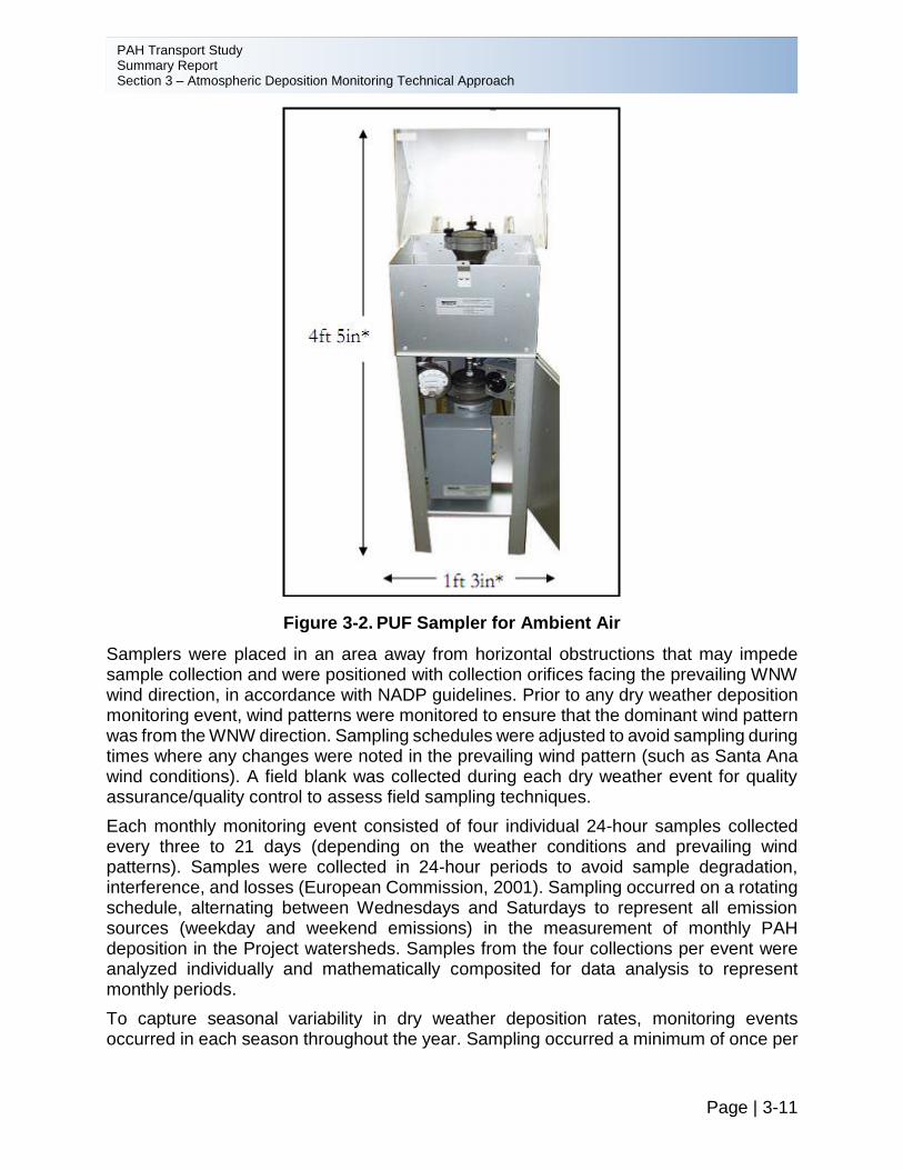
The samplers consist of a sample head inlet that contains the sampling media (precleaned and certified quartz filter and PUF/XAD-2® plug), a high-volume air blower that allows a large quantity of air to be drawn through the sampling media, and flow controllers and timers to quantify the sampling flow rates (Figure 3-2) (Tisch Environmental, 2012). The aerosol phase fractions of the PAHs are collected physically on the quartz fiber filter and the vapor phase fractions of the semi-volatile compounds are adsorbed on the sorbent (PUF/XAD-2®) cartridge sampling media. Detailed specifications of the HVAS, Quartz Filter and PUF/XAD-2® Adsorbent Cartridge, and GC/MS analysis under USEPA Method TO-13A are included in the Project QAPP (Appendix A).
The HVAS pulls ambient air through the filter/sorbent cartridge at a flow rate of approximately 8 cubic feet per minute (cfm) (0.225 cubic meter per minute [m3/min]) to obtain a total sample volume of greater than 300 cubic meters (m3) over a 24-hour period. The minimum flow rate for a given monitoring duration is calculated in (Equation 3-1):
𝑀𝑖𝑛𝐹𝑙𝑜𝑤𝑅𝑎𝑡𝑒 =
𝑀𝑖𝑛𝑆𝑎𝑚𝑝𝑙𝑒𝑉𝑜𝑙𝑢𝑚𝑒
𝑀𝑜𝑛𝑖𝑡𝑜𝑟𝑖𝑛𝑔𝐷𝑢𝑟𝑎𝑡𝑖𝑜𝑛
Equation 3-1
where:
MinFlowRate is the minimum flow rate (liters per minute [L/min]);
MinSampleVolume is the minimum sample volume (L) which was 300,000 liters (L) (= 300 m3); and
MonitoringDuration is the desired monitoring duration (minutes [min]), which was 1440 minutes (=24 hours).
PAH Transport Study Summary Report Section 3 – Atmospheric Deposition Monitoring Technical Approach
Page | 3-11
Figure 3-2. PUF Sampler for Ambient Air
Samplers were placed in an area away from horizontal obstructions that may impede sample collection and were positioned with collection orifices facing the prevailing WNW wind direction, in accordance with NADP guidelines. Prior to any dry weather deposition monitoring event, wind patterns were monitored to ensure that the dominant wind pattern was from the WNW direction. Sampling schedules were adjusted to avoid sampling during times where any changes were noted in the prevailing wind pattern (such as Santa Ana wind conditions). A field blank was collected during each dry weather event for quality assurance/quality control to assess field sampling techniques.
Each monthly monitoring event consisted of four individual 24-hour samples collected every three to 21 days (depending on the weather conditions and prevailing wind patterns). Samples were collected in 24-hour periods to avoid sample degradation, interference, and losses (European Commission, 2001). Sampling occurred on a rotating schedule, alternating between Wednesdays and Saturdays to represent all emission sources (weekday and weekend emissions) in the measurement of monthly PAH deposition in the Project watersheds. Samples from the four collections per event were analyzed individually and mathematically composited for data analysis to represent monthly periods.
To capture seasonal variability in dry weather deposition rates, monitoring events occurred in each season throughout the year. Sampling occurred a minimum of once per
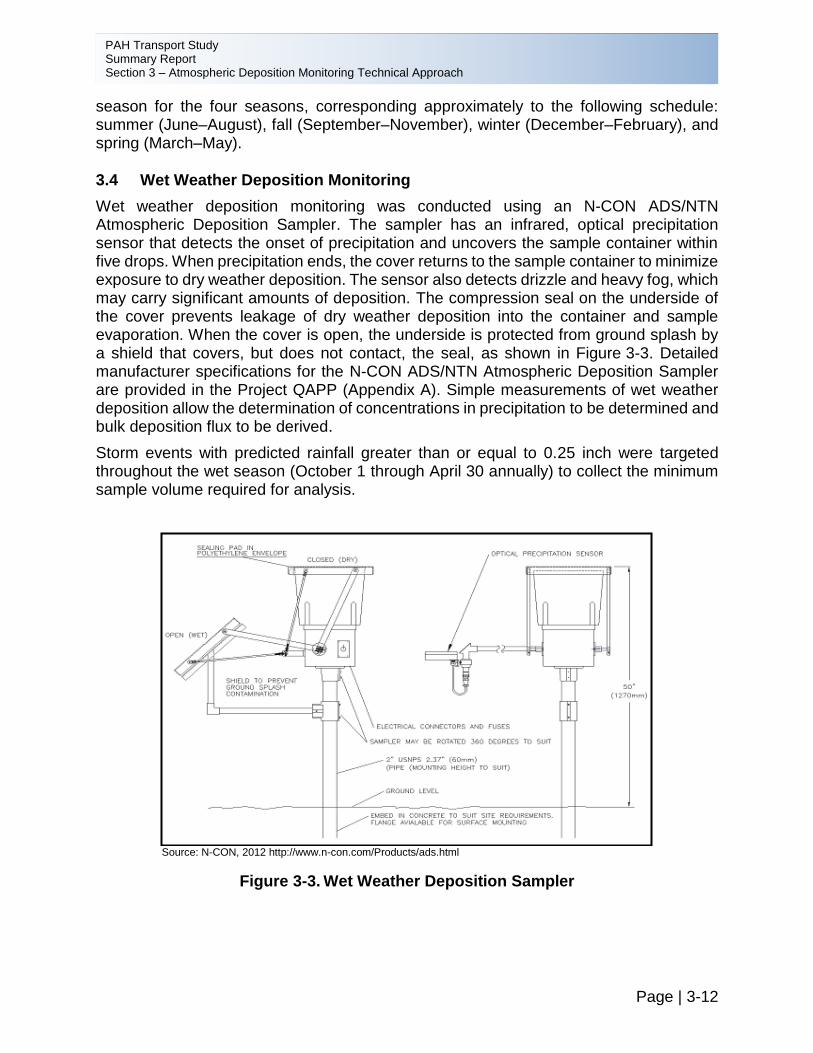
PAH Transport Study Summary Report Section 3 – Atmospheric Deposition Monitoring Technical Approach
Page | 3-12
season for the four seasons, corresponding approximately to the following schedule: summer (June–August), fall (September–November), winter (December–February), and spring (March–May).
3.4 Wet Weather Deposition Monitoring
Wet weather deposition monitoring was conducted using an N-CON ADS/NTN Atmospheric Deposition Sampler. The sampler has an infrared, optical precipitation sensor that detects the onset of precipitation and uncovers the sample container within five drops. When precipitation ends, the cover returns to the sample container to minimize exposure to dry weather deposition. The sensor also detects drizzle and heavy fog, which may carry significant amounts of deposition. The compression seal on the underside of the cover prevents leakage of dry weather deposition into the container and sample evaporation. When the cover is open, the underside is protected from ground splash by a shield that covers, but does not contact, the seal, as shown in Figure 3-3. Detailed manufacturer specifications for the N-CON ADS/NTN Atmospheric Deposition Sampler are provided in the Project QAPP (Appendix A). Simple measurements of wet weather deposition allow the determination of concentrations in precipitation to be determined and bulk deposition flux to be derived.
Storm events with predicted rainfall greater than or equal to 0.25 inch were targeted throughout the wet season (October 1 through April 30 annually) to collect the minimum sample volume required for analysis.
Source: N-CON, 2012 http://www.n-con.com/Products/ads.html
Figure 3-3. Wet Weather Deposition Sampler
PAH Transport Study Summary Report Section 3 – Atmospheric Deposition Monitoring Technical Approach
Page | 3-13
Intentionally Left Blank
PAH Transport Study Summary Report Section 4 – Results
Page | 4-1
4 RESULTS
To address the primary Project questions, data analysis was conducted to:
• Estimate the relative contribution of PAHs from the atmosphere via dry and wet deposition through loading calculations.
• Attempt to assign a source apportionment using results of the aerial deposition monitoring program and values from the literature review.
• Further characterize sources and identify the relative percent load contributed by each source, using diagnostic ratios and chemical fingerprinting.
Sections 4.1 through 4.7 summarize monitoring events and data analyses, including summary statistics, temporal patterns, spatial patterns, flux and loading estimations, source identification, and source apportionment.
The list of PAHs analyzed varied between the dry weather and wet weather monitoring programs because analytical different methods were available for the analysis of dry and wet deposition samples. To standardize the Project data analysis, the review focused on USEPA’s list of 16 priority pollutants (Section 1.1). These priority pollutants were used calculate the “total PAHs.” Results of the data analysis will be considered during development and implementation of future TMDLs.
4.1 Event Monitoring Summary
Project monitoring was completed from FY 2013–FY 2017. A total of six dry depositional and six wet depositional events were monitored at the reference site (Cabrillo National Monument [CNM1]) and the three transect sites (Fire Department [FD]07, FD11, and FD12). Five dry weather events and four wet weather events were completed under Phases I, II, and III. One additional dry depositional monitoring event and two wet weather events were conducted under during Phase IV to complete monitoring and reporting efforts for the Project. Phases I, II, and III were conducted during FY 2013–FY 2016 by the City. Phases IV and V were conducted during FY 2017–FY 2018 and were sponsored by the SWRCB under Agreement Number 15-064-190. The monitored events are summarized in Sections 4.1.1 and 4.1.2.
4.1.1 Dry Weather Deposition Sample Collections
As described in Section 2, to estimate the monthly dry weather deposition rate, monitoring events consisted of four sample collections spaced three to six days apart. Each sample collection was performed over a 24-hour period. Samples from the four collections per event were analyzed individually and mathematically composited for data analysis to represent monthly periods. These monthly periods were used to estimate an annual deposition.
Table 4-1 summarizes the six dry weather deposition monitoring events conducted by date, and the season during which samples were collected. Samples were collected over a 24-hour period, and the total air volume collected per sample ranged from 308 m3 to 336 m3.
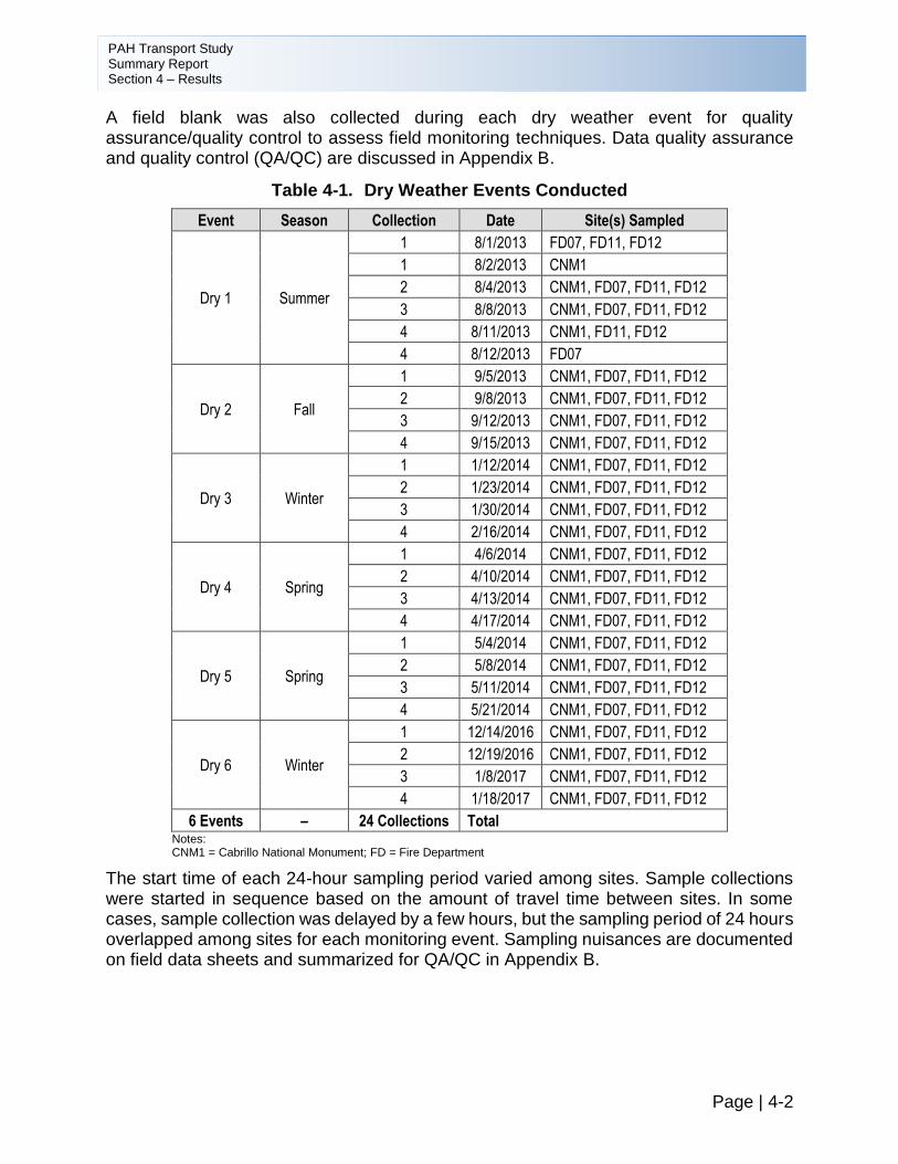
PAH Transport Study Summary Report Section 4 – Results
Page | 4-2
A field blank was also collected during each dry weather event for quality assurance/quality control to assess field monitoring techniques. Data quality assurance and quality control (QA/QC) are discussed in Appendix B.
Table 4-1. Dry Weather Events Conducted
Event Season Collection Date Site(s) Sampled
Dry 1 Summer
1 8/1/2013 FD07, FD11, FD12
1 8/2/2013 CNM1
2 8/4/2013 CNM1, FD07, FD11, FD12
3 8/8/2013 CNM1, FD07, FD11, FD12
4 8/11/2013 CNM1, FD11, FD12
4 8/12/2013 FD07
Dry 2 Fall
1 9/5/2013 CNM1, FD07, FD11, FD12
2 9/8/2013 CNM1, FD07, FD11, FD12
3 9/12/2013 CNM1, FD07, FD11, FD12
4 9/15/2013 CNM1, FD07, FD11, FD12
Dry 3 Winter
1 1/12/2014 CNM1, FD07, FD11, FD12
2 1/23/2014 CNM1, FD07, FD11, FD12
3 1/30/2014 CNM1, FD07, FD11, FD12
4 2/16/2014 CNM1, FD07, FD11, FD12
Dry 4 Spring
1 4/6/2014 CNM1, FD07, FD11, FD12
2 4/10/2014 CNM1, FD07, FD11, FD12
3 4/13/2014 CNM1, FD07, FD11, FD12
4 4/17/2014 CNM1, FD07, FD11, FD12
Dry 5 Spring
1 5/4/2014 CNM1, FD07, FD11, FD12
2 5/8/2014 CNM1, FD07, FD11, FD12
3 5/11/2014 CNM1, FD07, FD11, FD12
4 5/21/2014 CNM1, FD07, FD11, FD12
Dry 6 Winter
1 12/14/2016 CNM1, FD07, FD11, FD12
2 12/19/2016 CNM1, FD07, FD11, FD12
3 1/8/2017 CNM1, FD07, FD11, FD12
4 1/18/2017 CNM1, FD07, FD11, FD12
6 Events – 24 Collections Total Notes: CNM1 = Cabrillo National Monument; FD = Fire Department
The start time of each 24-hour sampling period varied among sites. Sample collections were started in sequence based on the amount of travel time between sites. In some cases, sample collection was delayed by a few hours, but the sampling period of 24 hours overlapped among sites for each monitoring event. Sampling nuisances are documented on field data sheets and summarized for QA/QC in Appendix B.
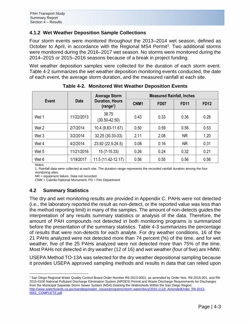
PAH Transport Study Summary Report Section 4 – Results
Page | 4-3
4.1.2 Wet Weather Deposition Sample Collections
Four storm events were monitored throughout the 2013–2014 wet season, defined as October to April, in accordance with the Regional MS4 Permit1. Two additional storms were monitored during the 2016–2017 wet season. No storms were monitored during the 2014–2015 or 2015–2016 seasons because of a break in project funding.
Wet weather deposition samples were collected for the duration of each storm event. Table 4-2 summarizes the wet weather deposition monitoring events conducted, the date of each event, the average storm duration, and the measured rainfall at each site.
Table 4-2. Monitored Wet Weather Deposition Events
Event Date Average Storm Duration, Hours
(range1)
Measured Rainfall, Inches
CNM1 FD07 FD11 FD12
Wet 1 11/22/2013 38.75
(30.50-42.50) 0.43 0.33 0.36 0.28
Wet 2 2/7/2014 10.4 (9.83-11.67) 0.50 0.59 0.56 0.53
Wet 3 3/2/2014 32.25 (30.33-33) 2.11 2.08 NR 1.20
Wet 4 4/2/2014 23.92 (22.5-24.5) 0.08 0.16 NR 0.31
Wet 5 11/21/2016 15 (7-15.33) 0.26 0.24 0.32 0.21
Wet 6 1/19/2017 11.5 (11.42-12.17) 0.56 0.55 0.56 0.56 Notes: 1. Rainfall data were collected at each site. The duration range represents the recorded rainfall duration among the four monitoring sites. NR = equipment failure. Data not recorded. CNM = Cabrillo National Monument; FD = Fire Department
4.2 Summary Statistics
The dry and wet monitoring results are provided in Appendix C. PAHs were not detected (i.e., the laboratory reported the result as non-detect, or the reported value was less than the method reporting limit) in many of the samples. The amount of non-detects guides the interpretation of any results summary statistics or analysis of the data. Therefore, the amount of PAH compounds not detected in both monitoring programs is summarized before the presentation of the summary statistics. Table 4-3 summarizes the percentage of results that were non-detects for each analyte. For dry weather conditions, 16 of the 21 PAHs analyzed were not detected more than 74 percent (%) of the time, and for wet weather, five of the 25 PAHs analyzed were not detected more than 75% of the time. Most PAHs not detected in dry weather (12 of 16) and wet weather (four of five) are HMW.
USEPA Method TO-13A was selected for the dry weather depositional sampling because it provides USEPA approved sampling methods and results in data that can relied upon
1 San Diego Regional Water Quality Control Board Order Number R9-2013-0001, as amended by Order Nos. R9-2015-001, and R9-2015-0100 National Pollutant Discharge Elimination System (NPDES) Permit and Waste Discharge Requirements for Discharges from the Municipal Separate Storm Sewer System (MS4) Draining the Watersheds Within the San Diego Region. http://www.waterboards.ca.gov/sandiego/water_issues/programs/storm water/docs/2015-1118_AmendedOrder_R9-2013-0001_COMPLETE.pdf
PAH Transport Study Summary Report Section 4 – Results
Page | 4-4
for accuracy. However, it is hypothesized after reviewing the large number of PAH compounds not detected during dry weather monitoring that the USEPA Method TO-13A may not adequately quantify the particulate phase of the dry weather PAH concentrations because a large portion of the HMW PAHs were not detected. PAHs, especially those having vapor pressures above 10–8 kilopascal (kPa), may vaporize from particulate filters during sampling (ASTM, 2013). PAH vapor pressures range from 1.1 × 10⁻² kPa for naphthalene to 2 × 10–13 kPa for coronene at 25 degrees Celsius (°C), which will dictate the phase in which PAHs will be present in ambient air. Although the analytical method permits collection and analysis of both the gaseous and particulate-phase PAHs, particulate-phase PAHs tend to be lost from the particulate filter during sampling because of desorption and volatilization. USEPA Method TO-13A does not permit the separate analysis of the particle and vapor phases. However, a modified method may allow for this alternative, as shown in other local studies (Sabin et al., 2004). Furthermore, a more recent method (2013) suggests that a backup vapor trap should be used for efficient sampling. However, this method still analyzes particulate and vapor (gaseous) phase PAHs together. Separate analyses of the filter and vapor trap will not reflect the original atmospheric phase distributions and therefore is not recommended (ASTM, 2013).
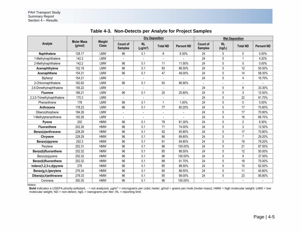
PAH Transport Study Summary Report Section 4 – Results
Page | 4-5
Table 4-3. Non-Detects per Analyte for Project Samples
Analyte Molar Mass
(g/mol) Weight Class
Dry Deposition Wet Deposition
Count of Samples
RL (µg/m3)
Total ND Percent ND Count of Samples
RL (ng/L)
Total ND Percent ND
Naphthalene 128.17 LMW 96 0.1 8 8.30% 24 5 0 0.00%
1-Methylnaphthalene 142.2 LMW - - - - 24 5 1 4.20%
2-Methylnaphthalene 142.2 LMW 96 0.1 11 11.50% 24 5 0 0.00%
Acenaphthylene 152.19 LMW 96 0.1 83 86.50% 24 5 12 50.00%
Acenaphthene 154.21 LMW 96 0.1 47 49.00% 24 5 14 58.30%
Biphenyl 154.21 LMW - - - - 24 5 4 16.70%
2-Chloronaphthalene 162.62 LMW 96 0.1 93 96.90% - - - -
2,6-Dimethylnaphthalene 156.22 LMW - - - - 24 5 8 33.30%
Fluorene 166.21 LMW 96 0.1 20 20.80% 24 5 3 12.50%
2,3,5-Trimethylnaphthalene 170.3 LMW - - - - 24 5 22 91.70%
Phenanthrene 178 LMW 96 0.1 1 1.00% 24 5 0 0.00%
Anthracene 178.23 LMW 96 0.1 77 80.20% 24 5 17 70.80%
Dibenzothiophene 184.26 LMW - - - - 24 5 17 70.80%
1-Methylphenanthrene 192.26 LMW - - - - 24 5 16 66.70%
Pyrene 202 HMW 96 0.1 78 81.30% 24 5 2 8.30%
Fluoranthene 202.26 HMW 96 0.1 71 74.00% 24 5 3 12.50%
Benzo(a)anthracene 228.29 HMW 96 0.1 92 95.80% 24 5 17 70.80%
Chrysene 228.29 HMW 96 0.1 86 89.60% 24 5 7 29.20%
Benzo(a)pyrene 252.3 HMW 96 0.1 91 94.80% 24 5 19 79.20%
Perylene 252.31 HMW 96 0.1 96 100.00% 24 5 21 87.50%
Benzo(b)fluoranthene 252.32 HMW 96 0.1 85 88.50% 24 5 12 50.00%
Benzo(e)pyrene 252.32 HMW 96 0.1 96 100.00% 24 5 9 37.50%
Benzo(k)fluoranthene 252.32 HMW 96 0.1 88 91.70% 24 5 18 75.00%
Indeno(1,2,3-c,d)pyrene 276 HMW 96 0.1 85 88.50% 24 5 15 62.50%
Benzo(g,h,i)perylene 276.34 HMW 96 0.1 85 88.50% 24 5 11 45.80%
Dibenz(a,h)anthracene 278.33 HMW 96 0.1 95 99.00% 24 5 23 95.80%
Coronene 300.35 HMW 96 0.1 96 100.00% - - - -
Notes: Bold indicates a USEPA priority pollutant, - = not analyzed, µg/m3 = micrograms per cubic meter; g/mol = grams per mole (molar mass); HMW = high molecular weight; LMW = low molecular weight; ND = non-detect; ng/L = nanograms per liter; RL = reporting limit

PAH Transport Study Summary Report Section 4 – Results
Page | 4-6
Intentionally Left Blank
PAH Transport Study Summary Report Section 4 – Results
Page | 4-7
Concentration data from dry deposition samples are presented in units of micrograms per cubic meter (µg/m3) and wet deposition sample results are presented in units of nanograms per liter (ng/L). These units are equivalent, allowing the two datasets to be compared with respect to mass to volume ratios (in different media, however). Basic summary statistics (maximum, minimum, mean with the standard deviation) are presented for PAHs analyzed as box plots in Figure 4-1 and are provided in Appendix D.
PAH concentrations typically were one to two orders of magnitude lower in dry weather results than in wet weather. Many of the HMW PAHs were not detected in the dry weather samples. Most PAHs were detected at very low concentrations or not detected. The only PAHs with consistent detections were naphthalene, dimethylnaphthalene, acenaphthene, fluorene, and phenanthrene.
The distribution of dry deposition results followed a similar pattern at all monitoring sites: the PAH concentrations in dry weather were lowest at the reference site (CNM1) and higher at the transect sites (FD07, FD11, and FD12; see Figure 4-1). Dry deposition concentrations, for the most part, were similar among transect sites. The distributions of PAH concentrations detected in wet deposition samples were more variable among sites than the distributions of PAH concentrations detected in dry deposition samples, which were mostly similar (Figure 4-1 compared to Figure 4-2). During wet weather conditions, PAH concentrations were lowest at the reference site, compared with the transect sites, for all compounds except naphthalene, phenanthrene, and pyrene, which showed similar or higher average concentrations at the reference site potentially indicating a regional source of these PAH compounds.
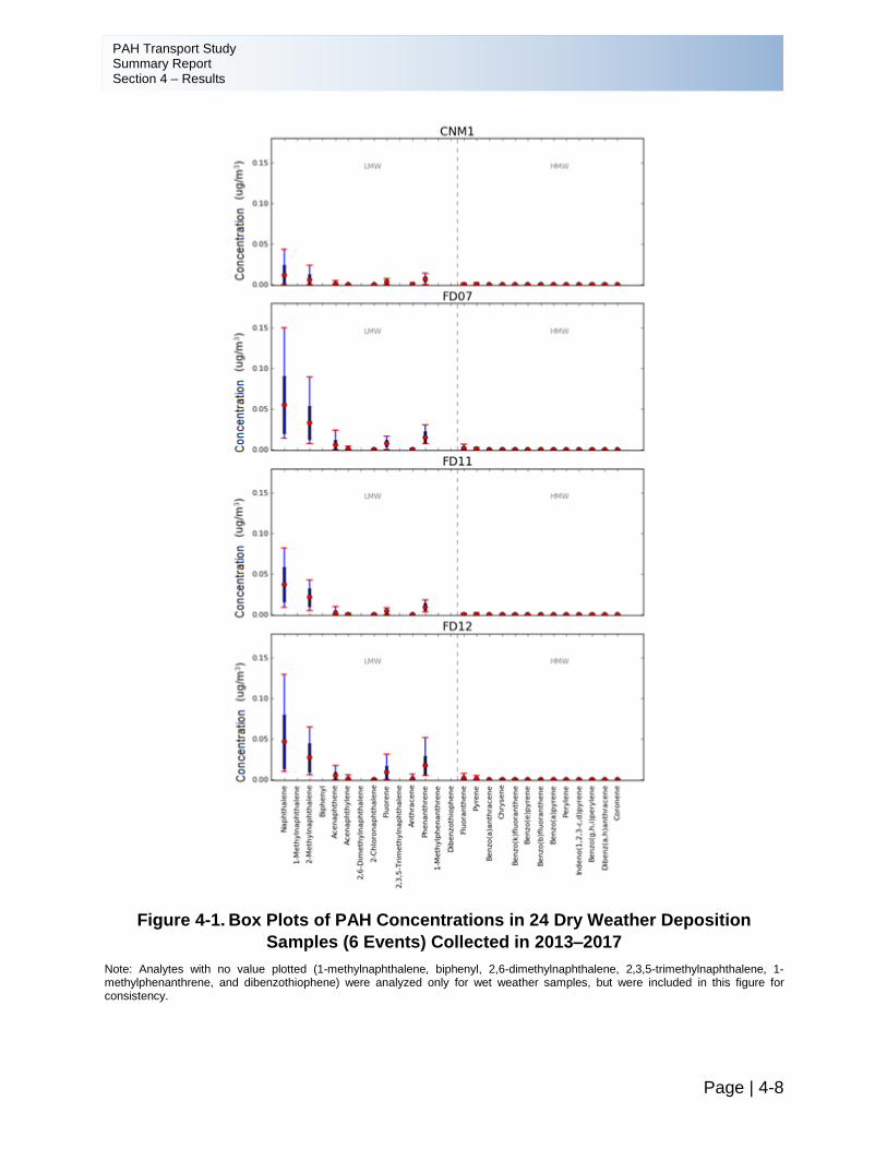
PAH Transport Study Summary Report Section 4 – Results
Page | 4-8
Figure 4-1. Box Plots of PAH Concentrations in 24 Dry Weather Deposition
Samples (6 Events) Collected in 2013–2017
Note: Analytes with no value plotted (1-methylnaphthalene, biphenyl, 2,6-dimethylnaphthalene, 2,3,5-trimethylnaphthalene, 1-methylphenanthrene, and dibenzothiophene) were analyzed only for wet weather samples, but were included in this figure for consistency.
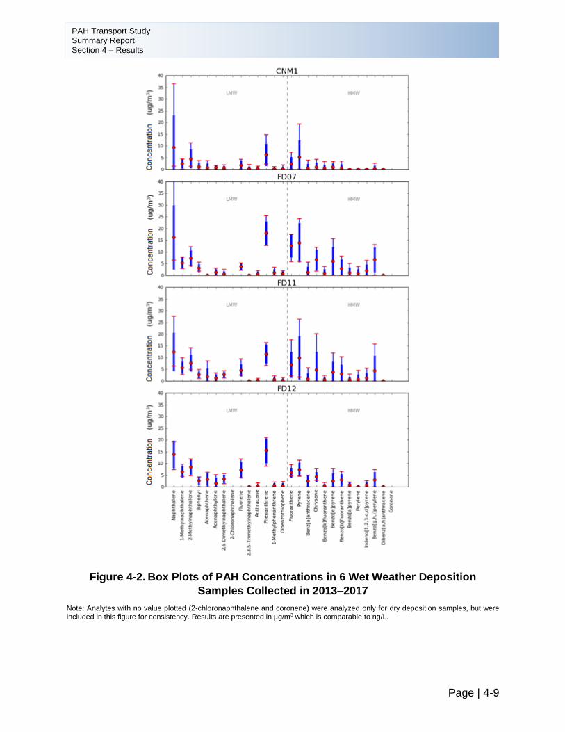
PAH Transport Study Summary Report Section 4 – Results
Page | 4-9
Figure 4-2. Box Plots of PAH Concentrations in 6 Wet Weather Deposition
Samples Collected in 2013–2017
Note: Analytes with no value plotted (2-chloronaphthalene and coronene) were analyzed only for dry deposition samples, but were included in this figure for consistency. Results are presented in µg/m3 which is comparable to ng/L.
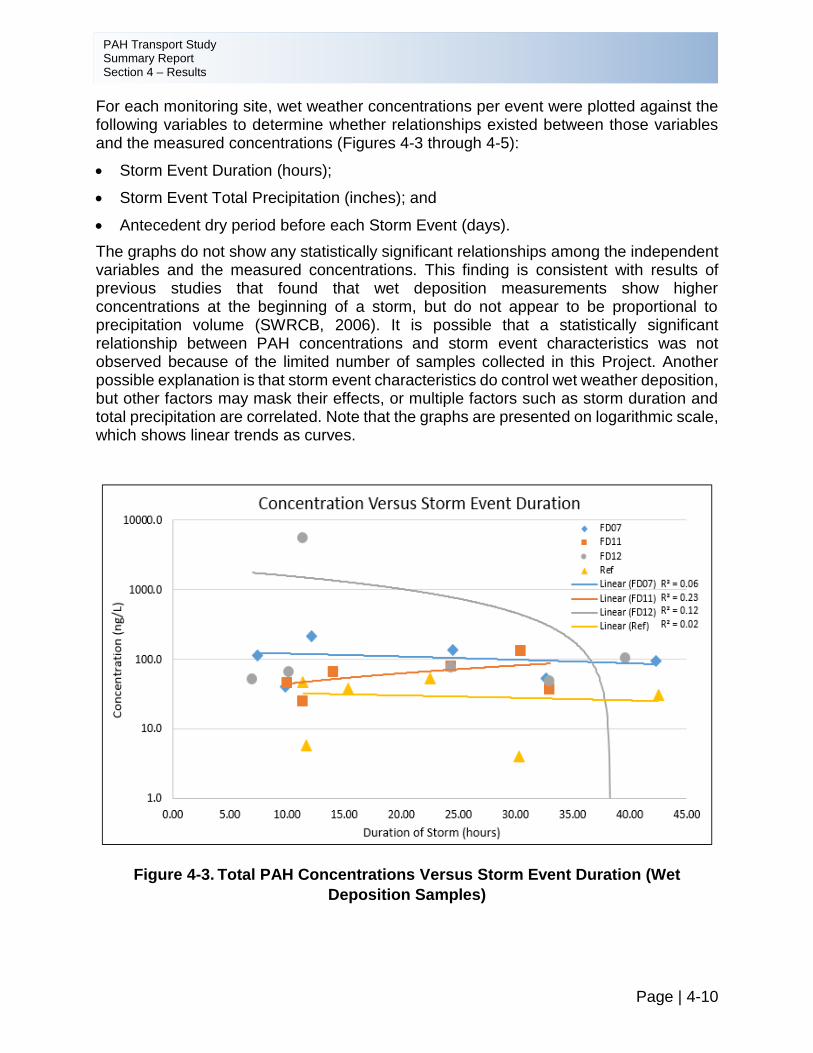
PAH Transport Study Summary Report Section 4 – Results
Page | 4-10
For each monitoring site, wet weather concentrations per event were plotted against the following variables to determine whether relationships existed between those variables and the measured concentrations (Figures 4-3 through 4-5):
• Storm Event Duration (hours);
• Storm Event Total Precipitation (inches); and
• Antecedent dry period before each Storm Event (days).
The graphs do not show any statistically significant relationships among the independent variables and the measured concentrations. This finding is consistent with results of previous studies that found that wet deposition measurements show higher concentrations at the beginning of a storm, but do not appear to be proportional to precipitation volume (SWRCB, 2006). It is possible that a statistically significant relationship between PAH concentrations and storm event characteristics was not observed because of the limited number of samples collected in this Project. Another possible explanation is that storm event characteristics do control wet weather deposition, but other factors may mask their effects, or multiple factors such as storm duration and total precipitation are correlated. Note that the graphs are presented on logarithmic scale, which shows linear trends as curves.
Figure 4-3. Total PAH Concentrations Versus Storm Event Duration (Wet
Deposition Samples)
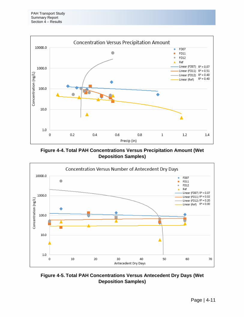
PAH Transport Study Summary Report Section 4 – Results
Page | 4-11
Figure 4-4. Total PAH Concentrations Versus Precipitation Amount (Wet
Deposition Samples)
Figure 4-5. Total PAH Concentrations Versus Antecedent Dry Days (Wet
Deposition Samples)
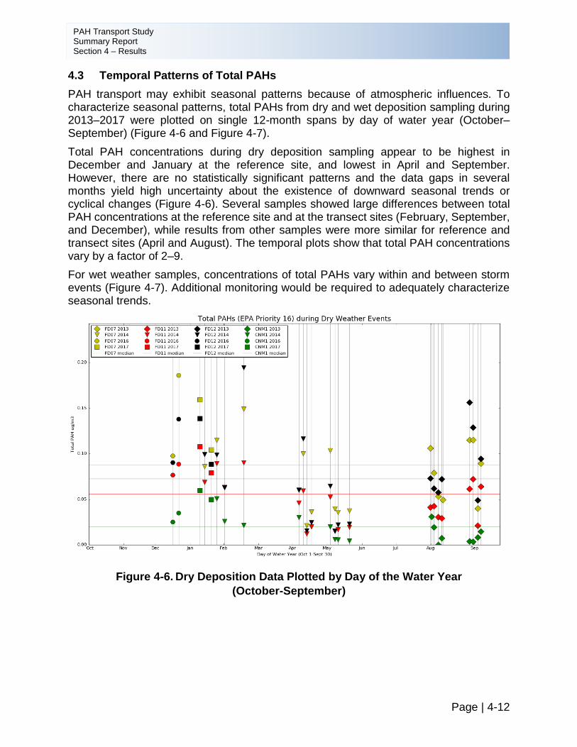
PAH Transport Study Summary Report Section 4 – Results
Page | 4-12
4.3 Temporal Patterns of Total PAHs
PAH transport may exhibit seasonal patterns because of atmospheric influences. To characterize seasonal patterns, total PAHs from dry and wet deposition sampling during 2013–2017 were plotted on single 12-month spans by day of water year (October–September) (Figure 4-6 and Figure 4-7).
Total PAH concentrations during dry deposition sampling appear to be highest in December and January at the reference site, and lowest in April and September. However, there are no statistically significant patterns and the data gaps in several months yield high uncertainty about the existence of downward seasonal trends or cyclical changes (Figure 4-6). Several samples showed large differences between total PAH concentrations at the reference site and at the transect sites (February, September, and December), while results from other samples were more similar for reference and transect sites (April and August). The temporal plots show that total PAH concentrations vary by a factor of 2–9.
For wet weather samples, concentrations of total PAHs vary within and between storm events (Figure 4-7). Additional monitoring would be required to adequately characterize seasonal trends.
Figure 4-6. Dry Deposition Data Plotted by Day of the Water Year
(October-September)
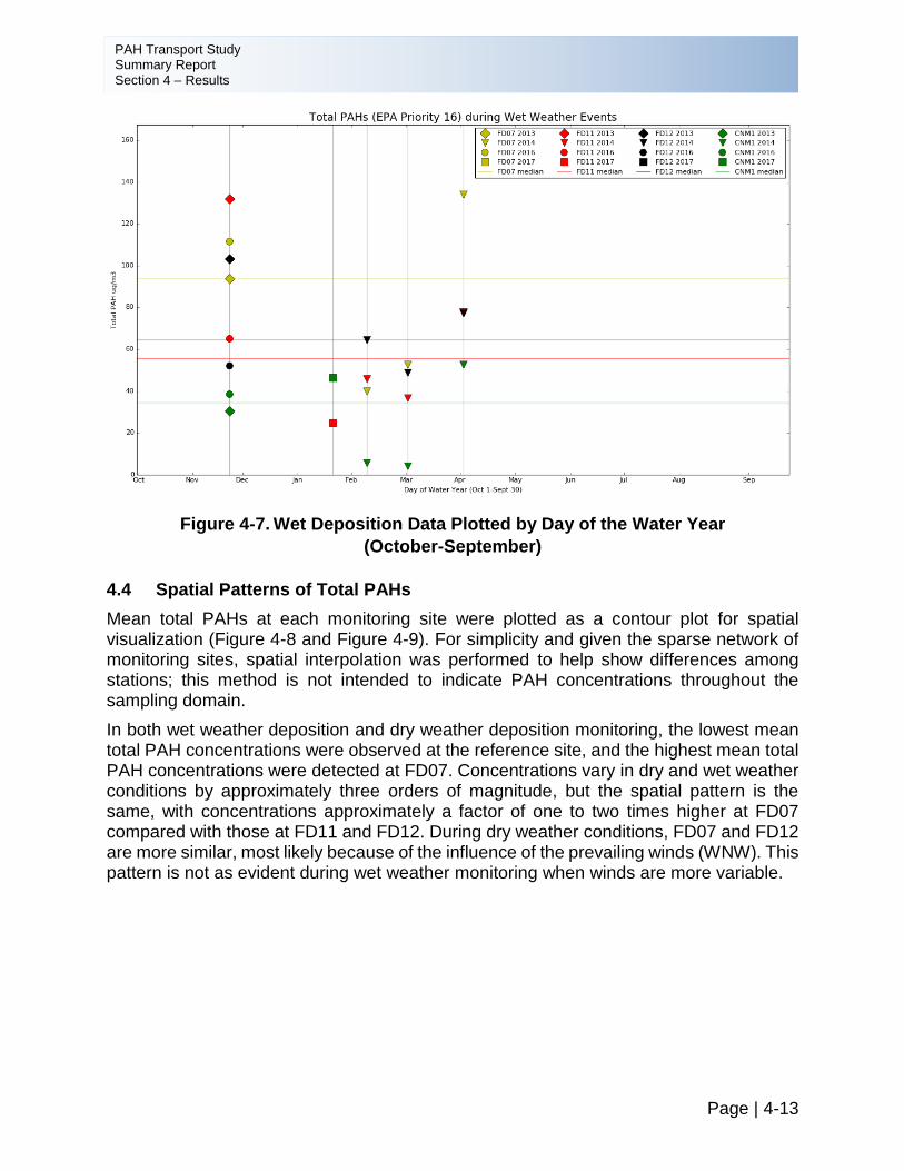
PAH Transport Study Summary Report Section 4 – Results
Page | 4-13
Figure 4-7. Wet Deposition Data Plotted by Day of the Water Year
(October-September)
4.4 Spatial Patterns of Total PAHs
Mean total PAHs at each monitoring site were plotted as a contour plot for spatial visualization (Figure 4-8 and Figure 4-9). For simplicity and given the sparse network of monitoring sites, spatial interpolation was performed to help show differences among stations; this method is not intended to indicate PAH concentrations throughout the sampling domain.
In both wet weather deposition and dry weather deposition monitoring, the lowest mean total PAH concentrations were observed at the reference site, and the highest mean total PAH concentrations were detected at FD07. Concentrations vary in dry and wet weather conditions by approximately three orders of magnitude, but the spatial pattern is the same, with concentrations approximately a factor of one to two times higher at FD07 compared with those at FD11 and FD12. During dry weather conditions, FD07 and FD12 are more similar, most likely because of the influence of the prevailing winds (WNW). This pattern is not as evident during wet weather monitoring when winds are more variable.
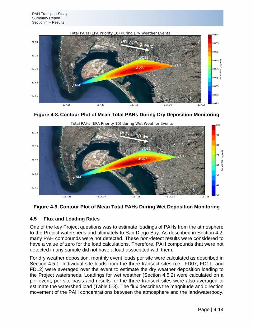
PAH Transport Study Summary Report Section 4 – Results
Page | 4-14
Figure 4-8. Contour Plot of Mean Total PAHs During Dry Deposition Monitoring
Figure 4-9. Contour Plot of Mean Total PAHs During Wet Deposition Monitoring
4.5 Flux and Loading Rates
One of the key Project questions was to estimate loadings of PAHs from the atmosphere to the Project watersheds and ultimately to San Diego Bay. As described in Section 4.2, many PAH compounds were not detected. These non-detect results were considered to have a value of zero for the load calculations. Therefore, PAH compounds that were not detected in any sample did not have a load associated with them.
For dry weather deposition, monthly event loads per site were calculated as described in Section 4.5.1. Individual site loads from the three transect sites (i.e., FD07, FD11, and FD12) were averaged over the event to estimate the dry weather deposition loading to the Project watersheds. Loadings for wet weather (Section 4.5.2) were calculated on a per-event, per-site basis and results for the three transect sites were also averaged to estimate the watershed load (Table 5-3). The flux describes the magnitude and direction movement of the PAH concentrations between the atmosphere and the land/waterbody.
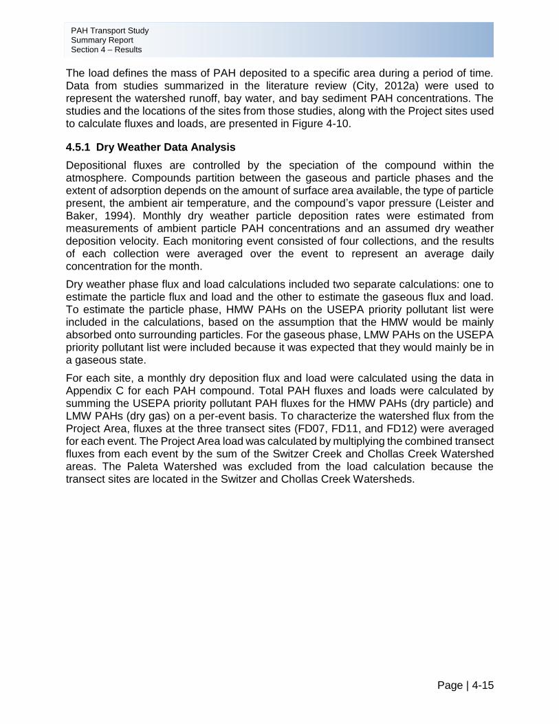
PAH Transport Study Summary Report Section 4 – Results
Page | 4-15
The load defines the mass of PAH deposited to a specific area during a period of time. Data from studies summarized in the literature review (City, 2012a) were used to represent the watershed runoff, bay water, and bay sediment PAH concentrations. The studies and the locations of the sites from those studies, along with the Project sites used to calculate fluxes and loads, are presented in Figure 4-10.
4.5.1 Dry Weather Data Analysis
Depositional fluxes are controlled by the speciation of the compound within the atmosphere. Compounds partition between the gaseous and particle phases and the extent of adsorption depends on the amount of surface area available, the type of particle present, the ambient air temperature, and the compound’s vapor pressure (Leister and Baker, 1994). Monthly dry weather particle deposition rates were estimated from measurements of ambient particle PAH concentrations and an assumed dry weather deposition velocity. Each monitoring event consisted of four collections, and the results of each collection were averaged over the event to represent an average daily concentration for the month.
Dry weather phase flux and load calculations included two separate calculations: one to estimate the particle flux and load and the other to estimate the gaseous flux and load. To estimate the particle phase, HMW PAHs on the USEPA priority pollutant list were included in the calculations, based on the assumption that the HMW would be mainly absorbed onto surrounding particles. For the gaseous phase, LMW PAHs on the USEPA priority pollutant list were included because it was expected that they would mainly be in a gaseous state.
For each site, a monthly dry deposition flux and load were calculated using the data in Appendix C for each PAH compound. Total PAH fluxes and loads were calculated by summing the USEPA priority pollutant PAH fluxes for the HMW PAHs (dry particle) and LMW PAHs (dry gas) on a per-event basis. To characterize the watershed flux from the Project Area, fluxes at the three transect sites (FD07, FD11, and FD12) were averaged for each event. The Project Area load was calculated by multiplying the combined transect fluxes from each event by the sum of the Switzer Creek and Chollas Creek Watershed areas. The Paleta Watershed was excluded from the load calculation because the transect sites are located in the Switzer and Chollas Creek Watersheds.

PAH Transport Study Summary Report Section 4 – Results
Page | 4-16
Intentionally Left Blank
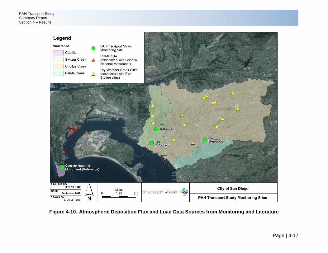
PAH Transport Study Summary Report Section 4 – Results
Page | 4-17
Figure 4-10. Atmospheric Deposition Flux and Load Data Sources from Monitoring and Literature

PAH Transport Study Summary Report Section 4 – Results
Page | 4-18
Intentionally Left Blank
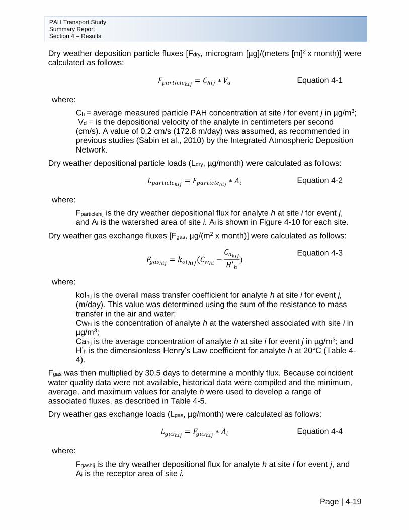
PAH Transport Study Summary Report Section 4 – Results
Page | 4-19
Dry weather deposition particle fluxes [Fdry, microgram [µg]/(meters [m]2 x month)] were calculated as follows:
𝐹𝑝𝑎𝑟𝑡𝑖𝑐𝑙𝑒ℎ𝑖𝑗= 𝐶ℎ𝑖𝑗 ∗ 𝑉𝑑 Equation 4-1
where:
Ch = average measured particle PAH concentration at site i for event j in µg/m3; Vd = is the depositional velocity of the analyte in centimeters per second (cm/s). A value of 0.2 cm/s (172.8 m/day) was assumed, as recommended in previous studies (Sabin et al., 2010) by the Integrated Atmospheric Deposition Network.
Dry weather depositional particle loads (Ldry, µg/month) were calculated as follows:
𝐿𝑝𝑎𝑟𝑡𝑖𝑐𝑙𝑒ℎ𝑖𝑗= 𝐹𝑝𝑎𝑟𝑡𝑖𝑐𝑙𝑒ℎ𝑖𝑗
∗ 𝐴𝑖 Equation 4-2
where:
Fparticlehij is the dry weather depositional flux for analyte h at site i for event j, and Ai is the watershed area of site i. Ai is shown in Figure 4-10 for each site.
Dry weather gas exchange fluxes [Fgas, µg/(m2 x month)] were calculated as follows:
𝐹𝑔𝑎𝑠ℎ𝑖𝑗
= 𝑘𝑜𝑙ℎ𝑖𝑗(𝐶𝑤ℎ𝑖
−𝐶𝑎ℎ𝑖𝑗
𝐻′ℎ)
Equation 4-3
where:
kolhij is the overall mass transfer coefficient for analyte h at site i for event j, (m/day). This value was determined using the sum of the resistance to mass transfer in the air and water; Cwhi is the concentration of analyte h at the watershed associated with site i in µg/m3; Cahij is the average concentration of analyte h at site i for event j in µg/m3; and H’h is the dimensionless Henry’s Law coefficient for analyte h at 20°C (Table 4-4).
Fgas was then multiplied by 30.5 days to determine a monthly flux. Because coincident water quality data were not available, historical data were compiled and the minimum, average, and maximum values for analyte h were used to develop a range of associated fluxes, as described in Table 4-5.
Dry weather gas exchange loads (Lgas, µg/month) were calculated as follows:
𝐿𝑔𝑎𝑠ℎ𝑖𝑗= 𝐹𝑔𝑎𝑠ℎ𝑖𝑗
∗ 𝐴𝑖 Equation 4-4
where:
Fgashij is the dry weather depositional flux for analyte h at site i for event j, and Ai is the receptor area of site i.
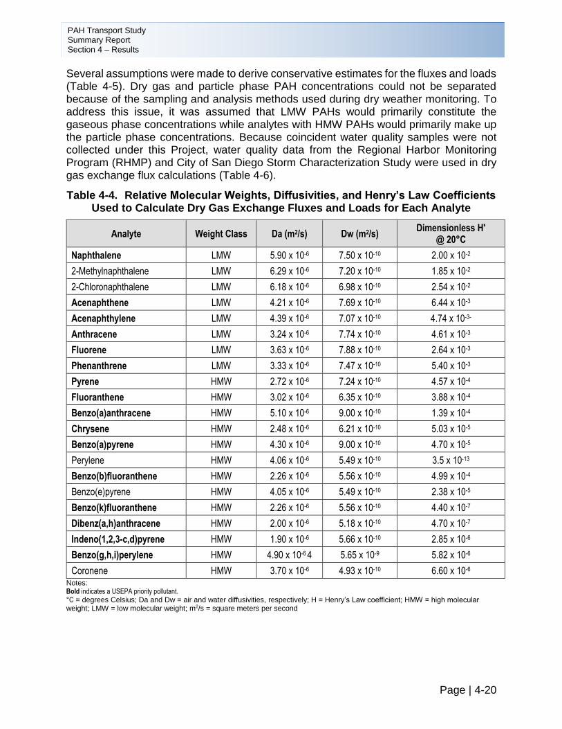
PAH Transport Study Summary Report Section 4 – Results
Page | 4-20
Several assumptions were made to derive conservative estimates for the fluxes and loads (Table 4-5). Dry gas and particle phase PAH concentrations could not be separated because of the sampling and analysis methods used during dry weather monitoring. To address this issue, it was assumed that LMW PAHs would primarily constitute the gaseous phase concentrations while analytes with HMW PAHs would primarily make up the particle phase concentrations. Because coincident water quality samples were not collected under this Project, water quality data from the Regional Harbor Monitoring Program (RHMP) and City of San Diego Storm Characterization Study were used in dry gas exchange flux calculations (Table 4-6).
Table 4-4. Relative Molecular Weights, Diffusivities, and Henry’s Law Coefficients Used to Calculate Dry Gas Exchange Fluxes and Loads for Each Analyte
Analyte Weight Class Da (m2/s) Dw (m2/s) Dimensionless H'
@ 20°C
Naphthalene LMW 5.90 x 10⁻⁶ 7.50 x 10⁻¹⁰ 2.00 x 10⁻²
2-Methylnaphthalene LMW 6.29 x 10⁻⁶ 7.20 x 10⁻¹⁰ 1.85 x 10⁻²
2-Chloronaphthalene LMW 6.18 x 10⁻⁶ 6.98 x 10⁻¹⁰ 2.54 x 10⁻²
Acenaphthene LMW 4.21 x 10⁻⁶ 7.69 x 10⁻¹⁰ 6.44 x 10⁻³
Acenaphthylene LMW 4.39 x 10⁻⁶ 7.07 x 10⁻¹⁰ 4.74 x 10⁻³-
Anthracene LMW 3.24 x 10⁻⁶ 7.74 x 10⁻¹⁰ 4.61 x 10⁻³
Fluorene LMW 3.63 x 10⁻⁶ 7.88 x 10⁻¹⁰ 2.64 x 10⁻³
Phenanthrene LMW 3.33 x 10⁻⁶ 7.47 x 10⁻¹⁰ 5.40 x 10⁻³
Pyrene HMW 2.72 x 10⁻⁶ 7.24 x 10⁻¹⁰ 4.57 x 10⁻⁴
Fluoranthene HMW 3.02 x 10⁻⁶ 6.35 x 10⁻¹⁰ 3.88 x 10⁻⁴
Benzo(a)anthracene HMW 5.10 x 10⁻⁶ 9.00 x 10⁻¹⁰ 1.39 x 10⁻⁴
Chrysene HMW 2.48 x 10⁻⁶ 6.21 x 10⁻¹⁰ 5.03 x 10⁻⁵
Benzo(a)pyrene HMW 4.30 x 10⁻⁶ 9.00 x 10⁻¹⁰ 4.70 x 10⁻⁵
Perylene HMW 4.06 x 10⁻⁶ 5.49 x 10⁻¹⁰ 3.5 x 10⁻¹³
Benzo(b)fluoranthene HMW 2.26 x 10⁻⁶ 5.56 x 10⁻¹⁰ 4.99 x 10⁻⁴
Benzo(e)pyrene HMW 4.05 x 10⁻⁶ 5.49 x 10⁻¹⁰ 2.38 x 10⁻⁵
Benzo(k)fluoranthene HMW 2.26 x 10⁻⁶ 5.56 x 10⁻¹⁰ 4.40 x 10⁻⁷
Dibenz(a,h)anthracene HMW 2.00 x 10⁻⁶ 5.18 x 10⁻¹⁰ 4.70 x 10⁻⁷
Indeno(1,2,3-c,d)pyrene HMW 1.90 x 10⁻⁶ 5.66 x 10⁻¹⁰ 2.85 x 10⁻⁶
Benzo(g,h,i)perylene HMW 4.90 x 10⁻⁶ 4 5.65 x 10⁻⁹ 5.82 x 10⁻⁶
Coronene HMW 3.70 x 10⁻⁶ 4.93 x 10⁻¹⁰ 6.60 x 10⁻⁶ Notes: Bold indicates a USEPA priority pollutant. °C = degrees Celsius; Da and Dw = air and water diffusivities, respectively; H = Henry’s Law coefficient; HMW = high molecular weight; LMW = low molecular weight; m2/s = square meters per second
PAH Transport Study Summary Report Section 4 – Results
Page | 4-21
Table 4-5. Assumptions for Dry Weather Flux and Load Estimations
Issue Assumption Made to Address Issue
Sampling method and analysis could not isolate particulate and gaseous phase PAHs
Fluxes were calculated on the basis of relative molecular weight. It was assumed HMW PAHs composed most of the dry particle depositional flux, LMW PAHs composed most of the dry gas exchange flux. The total PAH fluxes are based on the 16 USEPA priority pollutants and are segregated into their analyses by their weights for dry weather conditions. Total PAHs for wet weather results consist of all 16 priority pollutant PAHs together.
No coincident water quality data for dry gas exchange flux
Historical water quality data were used to calculate the gas exchange fluxes. Data for the CNM1 calculations came from the Regional Harbor Monitoring Program (RHMP) dataset from 2013 for San Diego Bay. Data for the transect sites came from the City of San Diego Storm Drain Characterization Study from 2009. Only creeks sampled as dry weather water quality sites within the watersheds of their corresponding PAH monitoring sites were used. Water quality data could not be obtained for 2-chloronapthalene or coronene because water samples collected under prior studies were not analyzed for these PAHs.
Wind speed measurements not taken concurrently with water quality data
Wind speeds measured at the PAH monitoring sites during each aerial deposition monitoring event were averaged over the monitoring event and used in the dry gas exchange flux calculations.
Missing weather station data
Because of power failures and/or weather station damage, some meteorological parameters were not measured for all events. In the case of missing rainfall data, values from neighboring sites were substituted for the calculations. In the case of missing wind speed data, data were downloaded from the Weather Underground website for the San Diego International Airport - Lindbergh Field weather station.
Values and/or equations necessary to develop the temperature-dependent molecular diffusivities and Henry's Law coefficients could not be found for each analyte for each event
Constant values for the molecular diffusivities and dimensionless Henry's Law Coefficients at 20 degrees Celsius were gathered from GSI Environmental’ s website.
Molecular diffusivity of water in air (DaH2O) could not be found/calculated
Based on the table of values in Datta, 2002. The value was interpolated using the function of a polynomial trend line developed in Microsoft Excel.
Molecular diffusivity of carbon dioxide in water (DwCO2) could not be found/calculated
Value was calculated on the basis of the Wilke-Chang equation using the following values and sources: Critical Volume of CO2 = 94 cubic centimeters per mole (cm3/mol) (http://www.apithailand.com/carbon.html)
Viscosity of water at 20 degrees Celsius = 1.002 millipascal seconds (mPa*s) (http://www.engineersedge.com/physics/water__density_viscosity_specific_weight_13146.htm)
Temperature = 293.15 K (calculation based on 20 degrees Celsius)
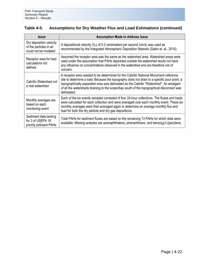
PAH Transport Study Summary Report Section 4 – Results
Table 4-5. Assumptions for Dry Weather Flux and Load Estimations (continued)
Page | 4-22
Issue Assumption Made to Address Issue
Dry deposition velocity of the particles in air could not be modeled
A depositional velocity (Vd) of 0.2 centimeters per second (cm/s) was used as recommended by the Integrated Atmospheric Deposition Network (Sabin et. al., 2010).
Receptor area for load calculations not defined
Assumed the receptor area was the same as the watershed area. Watershed areas were used under the assumption that PAHs deposited outside the watershed would not have any influence on concentrations observed in the watershed and are therefore not of concern.
Cabrillo Watershed not a real watershed
A receptor area needed to be determined for the Cabrillo National Monument reference site to determine a load. Because the topography does not drain to a specific pour point, a topographically separated area was delineated as the Cabrillo "Watershed". An amalgam of all the watersheds draining to the ocean/bay south of the topographical disconnect was delineated.
Monthly averages are based on each monitoring event
Each of the six events sampled consisted of four 24-hour collections. The fluxes and loads were calculated for each collection and were averaged over each monthly event. These six monthly averages were then averaged again to determine an average monthly flux and load for both the dry particle and dry gas depositions.
Sediment data lacking for 3 of USEPA 16 priority pollutant PAHs
Total PAHs for sediment fluxes are based on the remaining 13 PAHs for which data were available. Missing analytes are acenaphthalene, phenanthrene, and benzo(g,h,i)perylene.
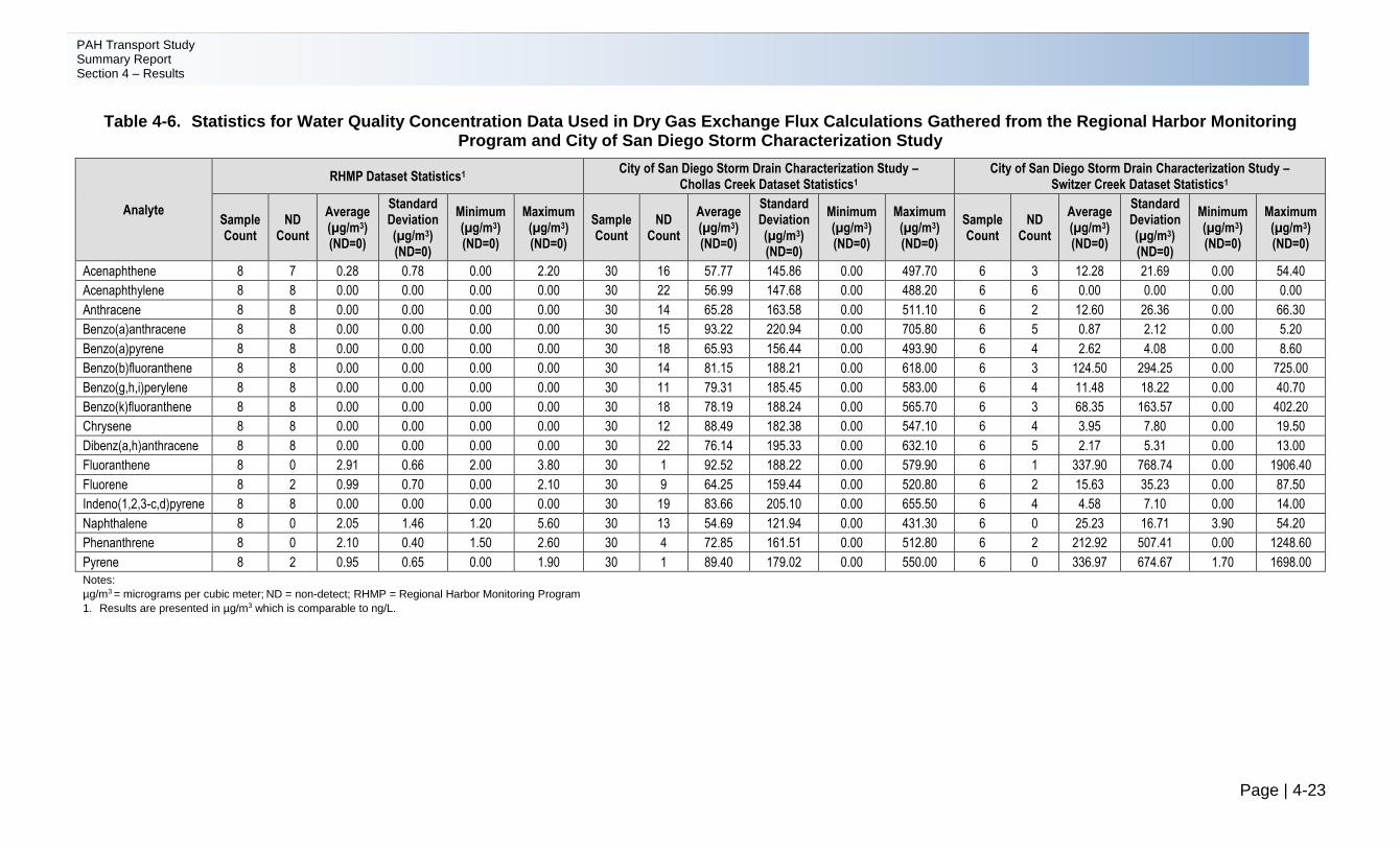
PAH Transport Study Summary Report Section 4 – Results
Page | 4-23
Table 4-6. Statistics for Water Quality Concentration Data Used in Dry Gas Exchange Flux Calculations Gathered from the Regional Harbor Monitoring Program and City of San Diego Storm Characterization Study
Analyte
RHMP Dataset Statistics1 City of San Diego Storm Drain Characterization Study –
Chollas Creek Dataset Statistics1 City of San Diego Storm Drain Characterization Study –
Switzer Creek Dataset Statistics1
Sample Count
ND Count
Average (µg/m3) (ND=0)
Standard Deviation (µg/m3) (ND=0)
Minimum (µg/m3) (ND=0)
Maximum (µg/m3) (ND=0)
Sample Count
ND Count
Average (µg/m3) (ND=0)
Standard Deviation (µg/m3) (ND=0)
Minimum (µg/m3) (ND=0)
Maximum (µg/m3) (ND=0)
Sample Count
ND Count
Average (µg/m3) (ND=0)
Standard Deviation (µg/m3) (ND=0)
Minimum (µg/m3) (ND=0)
Maximum (µg/m3) (ND=0)
Acenaphthene 8 7 0.28 0.78 0.00 2.20 30 16 57.77 145.86 0.00 497.70 6 3 12.28 21.69 0.00 54.40
Acenaphthylene 8 8 0.00 0.00 0.00 0.00 30 22 56.99 147.68 0.00 488.20 6 6 0.00 0.00 0.00 0.00
Anthracene 8 8 0.00 0.00 0.00 0.00 30 14 65.28 163.58 0.00 511.10 6 2 12.60 26.36 0.00 66.30
Benzo(a)anthracene 8 8 0.00 0.00 0.00 0.00 30 15 93.22 220.94 0.00 705.80 6 5 0.87 2.12 0.00 5.20
Benzo(a)pyrene 8 8 0.00 0.00 0.00 0.00 30 18 65.93 156.44 0.00 493.90 6 4 2.62 4.08 0.00 8.60
Benzo(b)fluoranthene 8 8 0.00 0.00 0.00 0.00 30 14 81.15 188.21 0.00 618.00 6 3 124.50 294.25 0.00 725.00
Benzo(g,h,i)perylene 8 8 0.00 0.00 0.00 0.00 30 11 79.31 185.45 0.00 583.00 6 4 11.48 18.22 0.00 40.70
Benzo(k)fluoranthene 8 8 0.00 0.00 0.00 0.00 30 18 78.19 188.24 0.00 565.70 6 3 68.35 163.57 0.00 402.20
Chrysene 8 8 0.00 0.00 0.00 0.00 30 12 88.49 182.38 0.00 547.10 6 4 3.95 7.80 0.00 19.50
Dibenz(a,h)anthracene 8 8 0.00 0.00 0.00 0.00 30 22 76.14 195.33 0.00 632.10 6 5 2.17 5.31 0.00 13.00
Fluoranthene 8 0 2.91 0.66 2.00 3.80 30 1 92.52 188.22 0.00 579.90 6 1 337.90 768.74 0.00 1906.40
Fluorene 8 2 0.99 0.70 0.00 2.10 30 9 64.25 159.44 0.00 520.80 6 2 15.63 35.23 0.00 87.50
Indeno(1,2,3-c,d)pyrene 8 8 0.00 0.00 0.00 0.00 30 19 83.66 205.10 0.00 655.50 6 4 4.58 7.10 0.00 14.00
Naphthalene 8 0 2.05 1.46 1.20 5.60 30 13 54.69 121.94 0.00 431.30 6 0 25.23 16.71 3.90 54.20
Phenanthrene 8 0 2.10 0.40 1.50 2.60 30 4 72.85 161.51 0.00 512.80 6 2 212.92 507.41 0.00 1248.60
Pyrene 8 2 0.95 0.65 0.00 1.90 30 1 89.40 179.02 0.00 550.00 6 0 336.97 674.67 1.70 1698.00
Notes:
µg/m3 = micrograms per cubic meter; ND = non-detect; RHMP = Regional Harbor Monitoring Program
1. Results are presented in µg/m3 which is comparable to ng/L.
PAH Transport Study Summary Report Section 4 – Results
Page | 4-24
Intentionally Left Blank
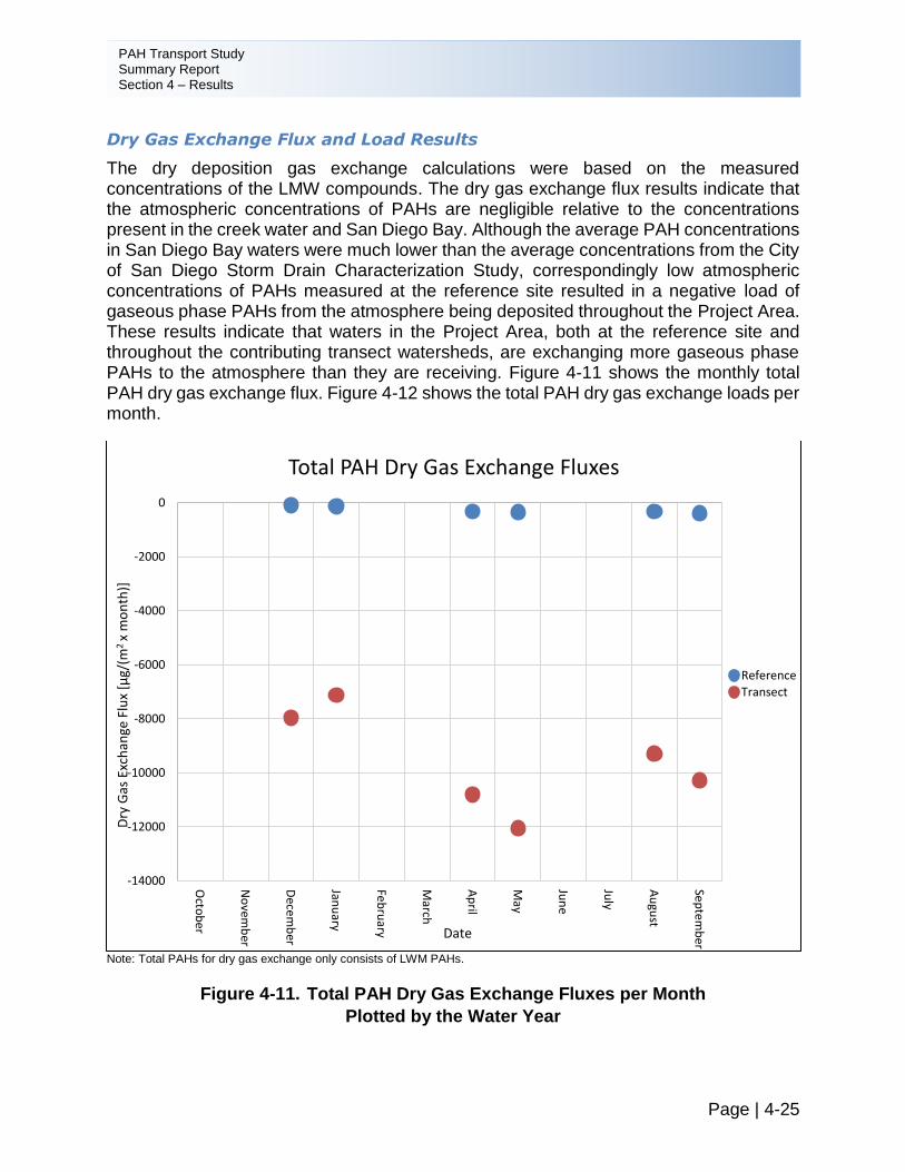
PAH Transport Study Summary Report Section 4 – Results
Page | 4-25
Dry Gas Exchange Flux and Load Results
The dry deposition gas exchange calculations were based on the measured concentrations of the LMW compounds. The dry gas exchange flux results indicate that the atmospheric concentrations of PAHs are negligible relative to the concentrations present in the creek water and San Diego Bay. Although the average PAH concentrations in San Diego Bay waters were much lower than the average concentrations from the City of San Diego Storm Drain Characterization Study, correspondingly low atmospheric concentrations of PAHs measured at the reference site resulted in a negative load of gaseous phase PAHs from the atmosphere being deposited throughout the Project Area. These results indicate that waters in the Project Area, both at the reference site and throughout the contributing transect watersheds, are exchanging more gaseous phase PAHs to the atmosphere than they are receiving. Figure 4-11 shows the monthly total PAH dry gas exchange flux. Figure 4-12 shows the total PAH dry gas exchange loads per month.
Note: Total PAHs for dry gas exchange only consists of LWM PAHs.
Figure 4-11. Total PAH Dry Gas Exchange Fluxes per Month
Plotted by the Water Year
-14000
-12000
-10000
-8000
-6000
-4000
-2000
0
Octo
be
r
No
vemb
er
Dece
mb
er
Janu
ary
Feb
ruary
March
Ap
ril
May
Jun
e
July
Au
gust
Sep
tem
ber
Dry
Gas
Exc
han
ge F
lux
[μg/
(m2
x m
on
th)]
Date
Total PAH Dry Gas Exchange Fluxes
ReferenceTransect
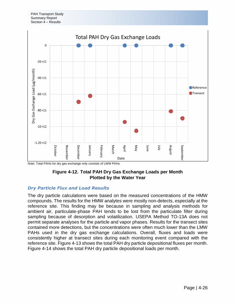
PAH Transport Study Summary Report Section 4 – Results
Page | 4-26
Note: Total PAHs for dry gas exchange only consists of LWM PAHs.
Figure 4-12. Total PAH Dry Gas Exchange Loads per Month
Plotted by the Water Year
Dry Particle Flux and Load Results
The dry particle calculations were based on the measured concentrations of the HMW compounds. The results for the HMW analytes were mostly non-detects, especially at the reference site. This finding may be because in sampling and analysis methods for ambient air, particulate-phase PAH tends to be lost from the particulate filter during sampling because of desorption and volatilization. USEPA Method TO-13A does not permit separate analyses for the particle and vapor phases. Results for the transect sites contained more detections, but the concentrations were often much lower than the LMW PAHs used in the dry gas exchange calculations. Overall, fluxes and loads were consistently higher at transect sites during each monitoring event compared with the reference site. Figure 4-13 shows the total PAH dry particle depositional fluxes per month. Figure 4-14 shows the total PAH dry particle depositional loads per month.
-1.2E+12
-1E+12
-8E+11
-6E+11
-4E+11
-2E+11
0
Octo
be
r
No
vemb
er
Dece
mb
er
Janu
ary
Feb
ruary
March
Ap
ril
May
Jun
e
July
Au
gust
Sep
tem
ber
Dry
Gas
Exc
han
ge L
oad
(μ
g/m
on
th)
Date
Total PAH Dry Gas Exchange Loads
Reference
Transect
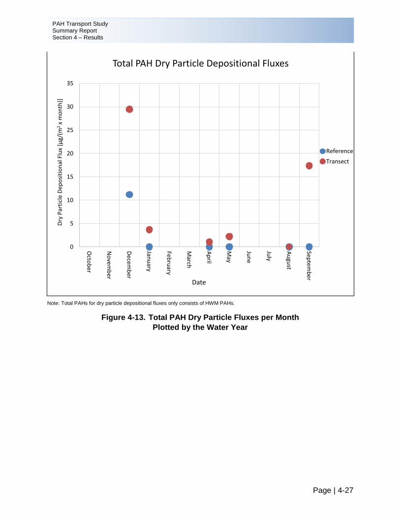
PAH Transport Study Summary Report Section 4 – Results
Page | 4-27
Note: Total PAHs for dry particle depositional fluxes only consists of HWM PAHs.
Figure 4-13. Total PAH Dry Particle Fluxes per Month
Plotted by the Water Year
0
5
10
15
20
25
30
35
Octo
be
r
No
vem
be
r
De
cemb
er
Janu
ary
Feb
ruary
March
Ap
ril
May
Jun
e
July
Au
gust
Sep
tem
be
r
Dry
Par
ticl
e D
epo
siti
on
al F
lux
[μg/
(m2
x m
on
th)]
Date
Total PAH Dry Particle Depositional Fluxes
Reference
Transect
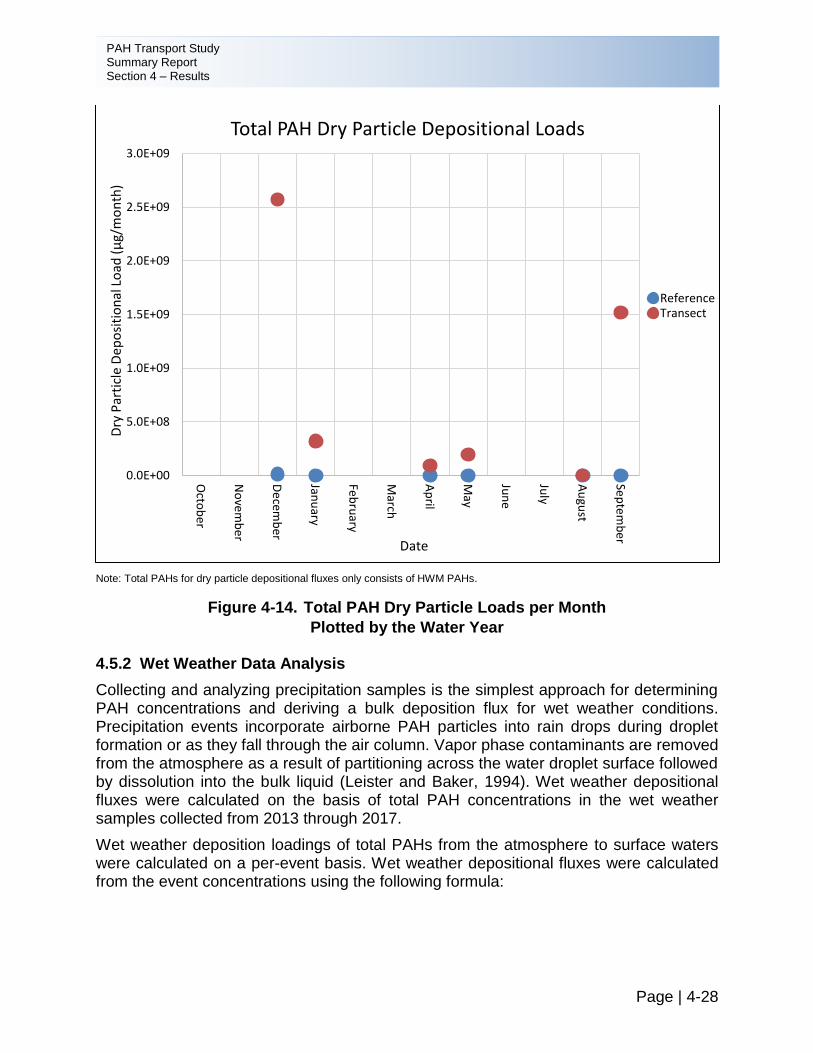
PAH Transport Study Summary Report Section 4 – Results
Page | 4-28
Note: Total PAHs for dry particle depositional fluxes only consists of HWM PAHs.
Figure 4-14. Total PAH Dry Particle Loads per Month
Plotted by the Water Year
4.5.2 Wet Weather Data Analysis
Collecting and analyzing precipitation samples is the simplest approach for determining PAH concentrations and deriving a bulk deposition flux for wet weather conditions. Precipitation events incorporate airborne PAH particles into rain drops during droplet formation or as they fall through the air column. Vapor phase contaminants are removed from the atmosphere as a result of partitioning across the water droplet surface followed by dissolution into the bulk liquid (Leister and Baker, 1994). Wet weather depositional fluxes were calculated on the basis of total PAH concentrations in the wet weather samples collected from 2013 through 2017.
Wet weather deposition loadings of total PAHs from the atmosphere to surface waters were calculated on a per-event basis. Wet weather depositional fluxes were calculated from the event concentrations using the following formula:
0.0E+00
5.0E+08
1.0E+09
1.5E+09
2.0E+09
2.5E+09
3.0E+09
Octo
be
r
No
vem
be
r
De
cemb
er
Janu
ary
Feb
ruary
March
Ap
ril
May
Jun
e
July
Au
gust
Sep
tem
be
r
Dry
Par
ticl
e D
epo
siti
on
al L
oad
(μ
g/m
on
th)
Date
Total PAH Dry Particle Depositional Loads
ReferenceTransect
PAH Transport Study Summary Report Section 4 – Results
Page | 4-29
Fwet = Chij * (τij) Equation 5-1
where:
Chij = concentration of analyte h at site i, for event j;
τij = precipitation rate [m3/(m2 x event)] at site i, for event j.
Rainfall data were measured at each monitoring site for most events. Transect site FD11 was missing meteorological data for several events due to data download failures. In these instances, data from FD12 were used to complete the calculations.
Total PAH results were calculated by summing the fluxes of the 16 USEPA priority pollutant PAHs on a per-site, per-event basis. Total PAH loads for each site/event were calculated by multiplying the total flux by each site’s respective watershed area (receptor area).
The combined transect site fluxes were calculated using a distance-weighted average for each event. Transect loads were calculated by multiplying the distance-weighted average fluxes by the sum of the Switzer Creek and Chollas Creek watershed areas. Table 4-7 provides assumptions used to estimate wet weather fluxes and loads.
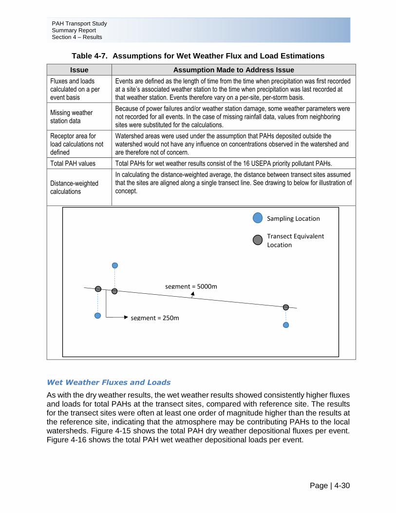
PAH Transport Study Summary Report Section 4 – Results
Page | 4-30
Table 4-7. Assumptions for Wet Weather Flux and Load Estimations
Issue Assumption Made to Address Issue
Fluxes and loads calculated on a per event basis
Events are defined as the length of time from the time when precipitation was first recorded at a site’s associated weather station to the time when precipitation was last recorded at that weather station. Events therefore vary on a per-site, per-storm basis.
Missing weather station data
Because of power failures and/or weather station damage, some weather parameters were not recorded for all events. In the case of missing rainfall data, values from neighboring sites were substituted for the calculations.
Receptor area for load calculations not defined
Watershed areas were used under the assumption that PAHs deposited outside the watershed would not have any influence on concentrations observed in the watershed and are therefore not of concern.
Total PAH values Total PAHs for wet weather results consist of the 16 USEPA priority pollutant PAHs.
Distance-weighted calculations
In calculating the distance-weighted average, the distance between transect sites assumed that the sites are aligned along a single transect line. See drawing to below for illustration of concept.
Wet Weather Fluxes and Loads
As with the dry weather results, the wet weather results showed consistently higher fluxes and loads for total PAHs at the transect sites, compared with reference site. The results for the transect sites were often at least one order of magnitude higher than the results at the reference site, indicating that the atmosphere may be contributing PAHs to the local watersheds. Figure 4-15 shows the total PAH dry weather depositional fluxes per event. Figure 4-16 shows the total PAH wet weather depositional loads per event.
Sampling Location
Transect Equivalent Location
segment = 5000m
segment = 250m
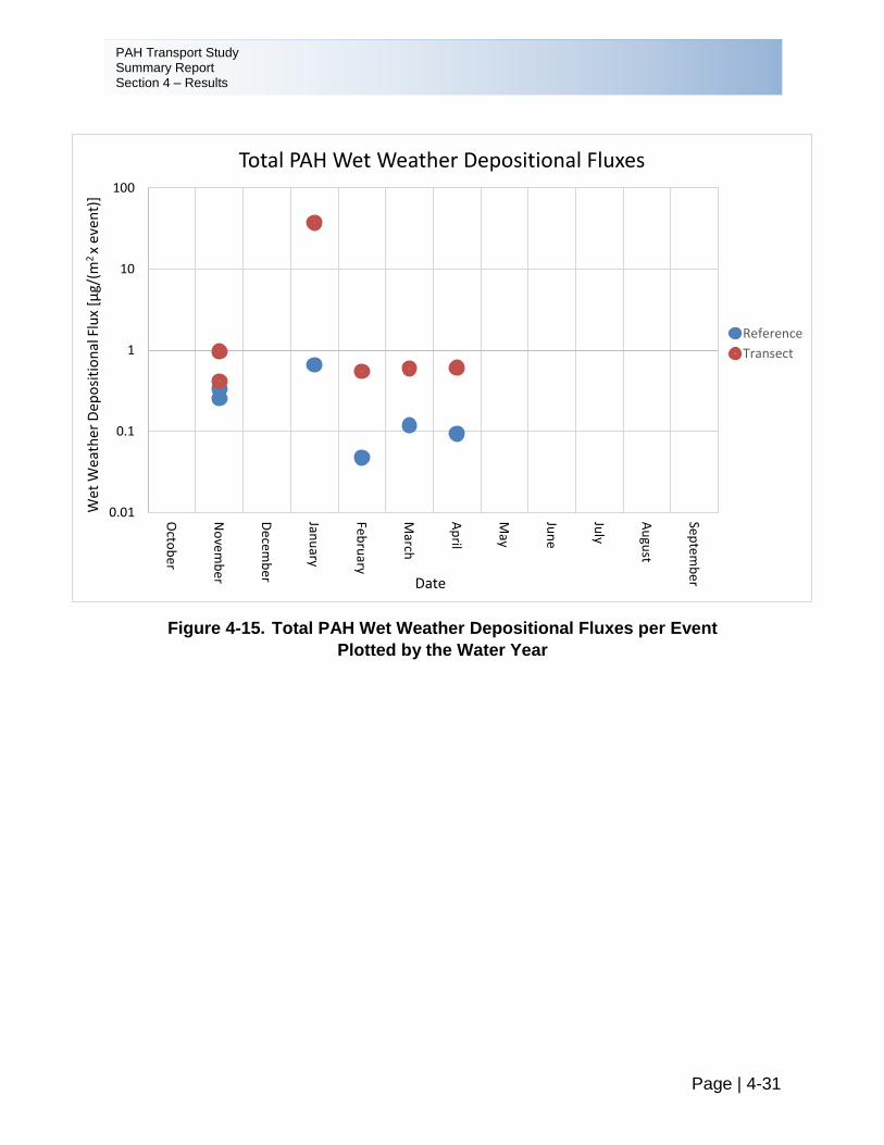
PAH Transport Study Summary Report Section 4 – Results
Page | 4-31
Figure 4-15. Total PAH Wet Weather Depositional Fluxes per Event
Plotted by the Water Year
0.01
0.1
1
10
100
Octo
be
r
No
vem
be
r
De
cemb
er
Janu
ary
Feb
ruary
March
Ap
ril
May
Jun
e
July
Au
gust
Sep
tem
be
r
We
t W
eat
her
Dep
osi
tio
nal
Flu
x [μ
g/(m
2 x
eve
nt)
]
Date
Total PAH Wet Weather Depositional Fluxes
Reference
Transect
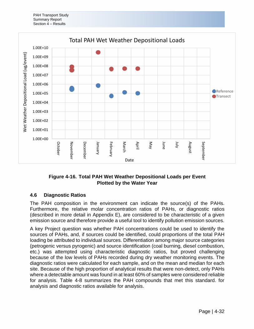
PAH Transport Study Summary Report Section 4 – Results
Page | 4-32
Figure 4-16. Total PAH Wet Weather Depositional Loads per Event
Plotted by the Water Year
4.6 Diagnostic Ratios
The PAH composition in the environment can indicate the source(s) of the PAHs. Furthermore, the relative molar concentration ratios of PAHs, or diagnostic ratios (described in more detail in Appendix E), are considered to be characteristic of a given emission source and therefore provide a useful tool to identify pollution emission sources.
A key Project question was whether PAH concentrations could be used to identify the sources of PAHs, and, if sources could be identified, could proportions of the total PAH loading be attributed to individual sources. Differentiation among major source categories (petrogenic versus pyrogenic) and source identification (coal burning, diesel combustion, etc.) was attempted using characteristic diagnostic ratios, but proved challenging because of the low levels of PAHs recorded during dry weather monitoring events. The diagnostic ratios were calculated for each sample, and on the mean and median for each site. Because of the high proportion of analytical results that were non-detect, only PAHs where a detectable amount was found in at least 60% of samples were considered reliable for analysis. Table 4-8 summarizes the PAH compounds that met this standard. for analysis and diagnostic ratios available for analysis.
1.00E+00
1.00E+01
1.00E+02
1.00E+03
1.00E+04
1.00E+05
1.00E+06
1.00E+07
1.00E+08
1.00E+09
1.00E+10
Octo
be
r
No
vem
be
r
De
cemb
er
Janu
ary
Feb
ruary
March
Ap
ril
May
Jun
e
July
Au
gust
Sep
tem
be
r
Wet
Wea
ther
Dep
osi
tio
nal
Lo
ad (
ug/
even
t)
Date
Total PAH Wet Weather Depositional Loads
ReferenceTransect
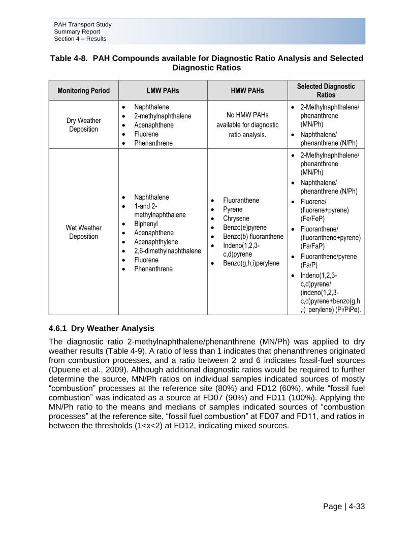
PAH Transport Study Summary Report Section 4 – Results
Page | 4-33
Table 4-8. PAH Compounds available for Diagnostic Ratio Analysis and Selected Diagnostic Ratios
4.6.1 Dry Weather Analysis
The diagnostic ratio 2-methylnaphthalene/phenanthrene (MN/Ph) was applied to dry weather results (Table 4-9). A ratio of less than 1 indicates that phenanthrenes originated from combustion processes, and a ratio between 2 and 6 indicates fossil-fuel sources (Opuene et al., 2009). Although additional diagnostic ratios would be required to further determine the source, MN/Ph ratios on individual samples indicated sources of mostly “combustion” processes at the reference site (80%) and FD12 (60%), while “fossil fuel combustion” was indicated as a source at FD07 (90%) and FD11 (100%). Applying the MN/Ph ratio to the means and medians of samples indicated sources of “combustion processes” at the reference site, “fossil fuel combustion” at FD07 and FD11, and ratios in between the thresholds (1<x<2) at FD12, indicating mixed sources.
Monitoring Period LMW PAHs HMW PAHs Selected Diagnostic
Ratios
Dry Weather Deposition
• Naphthalene
• 2-methylnaphthalene
• Acenaphthene
• Fluorene
• Phenanthrene
No HMW PAHs
available for diagnostic
ratio analysis.
• 2-Methylnaphthalene/ phenanthrene (MN/Ph)
• Naphthalene/ phenanthrene (N/Ph)
Wet Weather Deposition
• Naphthalene
• 1-and 2-methylnaphthalene
• Biphenyl
• Acenaphthene
• Acenaphthylene
• 2,6-dimethylnaphthalene
• Fluorene
• Phenanthrene
• Fluoranthene
• Pyrene
• Chrysene
• Benzo(e)pyrene
• Benzo(b) fluoranthene
• Indeno(1,2,3-c,d)pyrene
• Benzo(g,h,i)perylene
• 2-Methylnaphthalene/ phenanthrene (MN/Ph)
• Naphthalene/ phenanthrene (N/Ph)
• Fluorene/ (fluorene+pyrene) (Fe/FeP)
• Fluoranthene/ (fluoranthene+pyrene) (Fa/FaP)
• Fluoranthene/pyrene (Fa/P)
• Indeno(1,2,3-c,d)pyrene/ (indeno(1,2,3-c,d)pyrene+benzo(g,h,i) perylene) (Pi/PiPe).
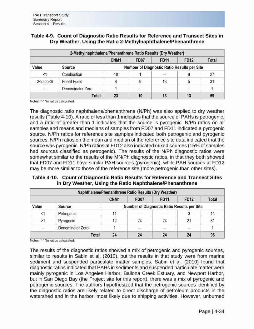
PAH Transport Study Summary Report Section 4 – Results
Page | 4-34
Table 4-9. Count of Diagnostic Ratio Results for Reference and Transect Sites in Dry Weather, Using the Ratio 2-Methylnaphthalene/Phenanthrene
2-Methylnaphthalene/Phenanthrene Ratio Results (Dry Weather)
CNM1 FD07 FD11 FD12 Total
Value Source Number of Diagnostic Ratio Results per Site
<1 Combustion 18 1 – 8 27
2<ratio<6 Fossil Fuels 4 9 13 5 31
- Denominator Zero 1 – – – 1
Total 23 10 13 13 59 Notes: “-“ No ratios calculated.
The diagnostic ratio naphthalene/phenanthrene (N/Ph) was also applied to dry weather results (Table 4-10). A ratio of less than 1 indicates that the source of PAHs is petrogenic, and a ratio of greater than 1 indicates that the source is pyrogenic. N/Ph ratios on all samples and means and medians of samples from FD07 and FD11 indicated a pyrogenic source. N/Ph ratios for reference site samples indicated both petrogenic and pyrogenic sources. N/Ph ratios on the mean and median of the reference site data indicated that the source was pyrogenic. N/Ph ratios at FD12 also indicated mixed sources (15% of samples had sources classified as petrogenic). The results of the N/Ph diagnostic ratios were somewhat similar to the results of the MN/Ph diagnostic ratios, in that they both showed that FD07 and FD11 have similar PAH sources (pyrogenic), while PAH sources at FD12 may be more similar to those of the reference site (more petrogenic than other sites).
Table 4-10. Count of Diagnostic Ratio Results for Reference and Transect Sites in Dry Weather, Using the Ratio Naphthalene/Phenanthrene
Naphthalene/Phenanthrene Ratio Results (Dry Weather)
CNM1 FD07 FD11 FD12 Total
Value Source Number of Diagnostic Ratio Results per Site
<1 Petrogenic 11 – – 3 14
>1 Pyrogenic 12 24 24 21 81
- Denominator Zero 1 – – – 1
Total 24 24 24 24 96 Notes: “-“ No ratios calculated.
The results of the diagnostic ratios showed a mix of petrogenic and pyrogenic sources, similar to results in Sabin et al. (2010), but the results in that study were from marine sediment and suspended particulate matter samples. Sabin et al. (2010) found that diagnostic ratios indicated that PAHs in sediments and suspended particulate matter were mainly pyrogenic in Los Angeles Harbor, Ballona Creek Estuary, and Newport Harbor, but in San Diego Bay (the Project site for this report), there was a mix of pyrogenic and petrogenic sources. The authors hypothesized that the petrogenic sources identified by the diagnostic ratios are likely related to direct discharge of petroleum products in the watershed and in the harbor, most likely due to shipping activities. However, unburned
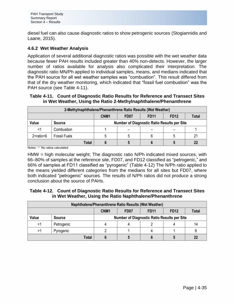
PAH Transport Study Summary Report Section 4 – Results
Page | 4-35
diesel fuel can also cause diagnostic ratios to show petrogenic sources (Stogiannidis and Laane, 2015).
4.6.2 Wet Weather Analysis
Application of several additional diagnostic ratios was possible with the wet weather data because fewer PAH results included greater than 40% non-detects. However, the larger number of ratios available for analysis also complicated their interpretation. The diagnostic ratio MN/Ph applied to individual samples, means, and medians indicated that the PAH source for all wet weather samples was “combustion”. This result differed from that of the dry weather monitoring, which indicated that “fossil fuel combustion” was the PAH source (see Table 4-11).
Table 4-11. Count of Diagnostic Ratio Results for Reference and Transect Sites in Wet Weather, Using the Ratio 2-Methylnaphthalene/Phenanthrene
2-Methylnaphthalene/Phenanthrene Ratio Results (Wet Weather)
CNM1 FD07 FD11 FD12 Total
Value Source Number of Diagnostic Ratio Results per Site
<1 Combustion 1 – – – 1
2<ratio<6 Fossil Fuels 5 5 6 5 21
Total 6 5 6 5 22 Notes: “-“ No ratios calculated.
HMW = high molecular weight; The diagnostic ratio N/Ph indicated mixed sources, with 66–80% of samples at the reference site, FD07, and FD12 classified as “petrogenic,” and 66% of samples at FD11 classified as “pyrogenic” (Table 4-12) The N/Ph ratio applied to the means yielded different categories from the medians for all sites but FD07, where both indicated “petrogenic” sources. The results of N/Ph ratios did not produce a strong conclusion about the source of PAHs.
Table 4-12. Count of Diagnostic Ratio Results for Reference and Transect Sites in Wet Weather, Using the Ratio Naphthalene/Phenanthrene
Naphthalene/Phenanthrene Ratio Results (Wet Weather)
CNM1 FD07 FD11 FD12 Total
Value Source Number of Diagnostic Ratio Results per Site
<1 Petrogenic 4 4 2 4 14
>1 Pyrogenic 2 1 4 1 8
Total 6 5 6 5 22
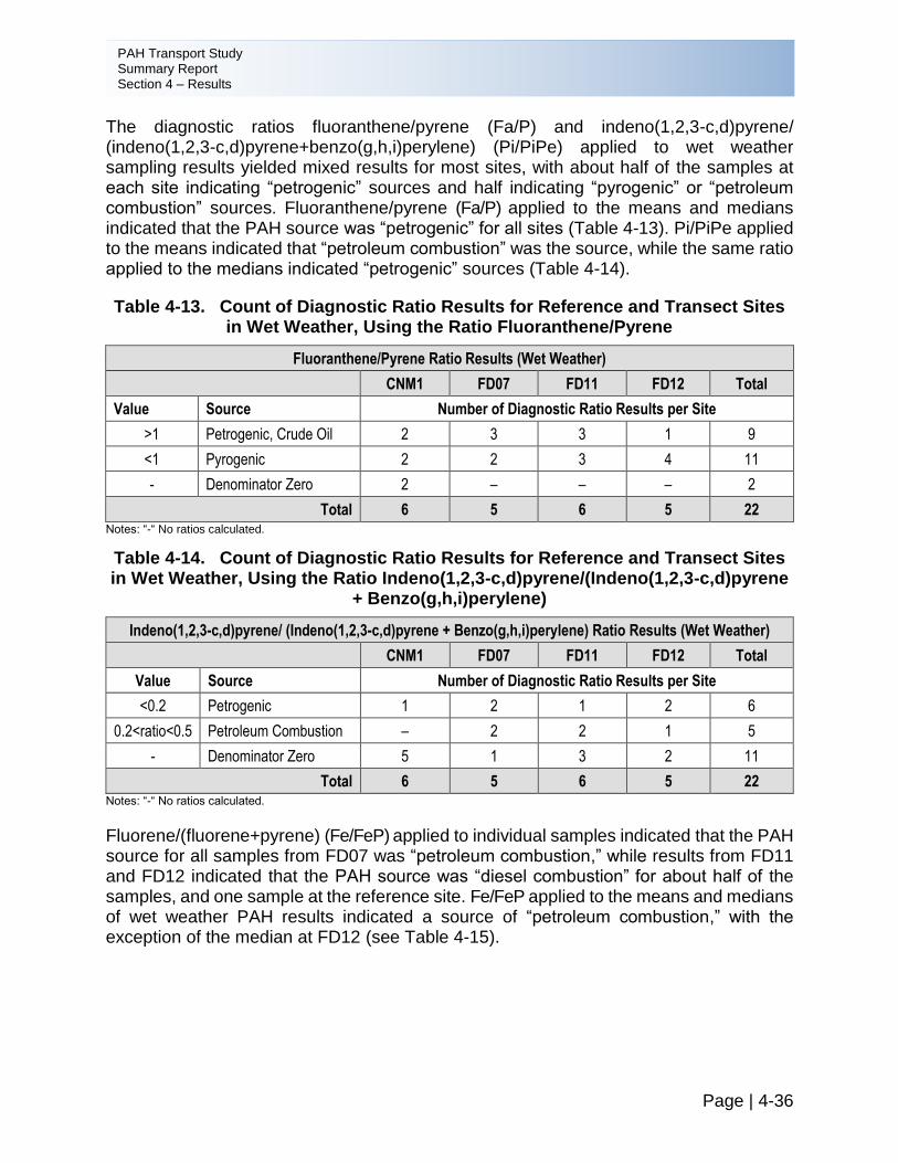
PAH Transport Study Summary Report Section 4 – Results
Page | 4-36
The diagnostic ratios fluoranthene/pyrene (Fa/P) and indeno(1,2,3-c,d)pyrene/ (indeno(1,2,3-c,d)pyrene+benzo(g,h,i)perylene) (Pi/PiPe) applied to wet weather sampling results yielded mixed results for most sites, with about half of the samples at each site indicating “petrogenic” sources and half indicating “pyrogenic” or “petroleum combustion” sources. Fluoranthene/pyrene (Fa/P) applied to the means and medians indicated that the PAH source was “petrogenic” for all sites (Table 4-13). Pi/PiPe applied to the means indicated that “petroleum combustion” was the source, while the same ratio applied to the medians indicated “petrogenic” sources (Table 4-14).
Table 4-13. Count of Diagnostic Ratio Results for Reference and Transect Sites in Wet Weather, Using the Ratio Fluoranthene/Pyrene
Fluoranthene/Pyrene Ratio Results (Wet Weather)
CNM1 FD07 FD11 FD12 Total
Value Source Number of Diagnostic Ratio Results per Site
>1 Petrogenic, Crude Oil 2 3 3 1 9
<1 Pyrogenic 2 2 3 4 11
- Denominator Zero 2 – – – 2
Total 6 5 6 5 22 Notes: “-“ No ratios calculated.
Table 4-14. Count of Diagnostic Ratio Results for Reference and Transect Sites in Wet Weather, Using the Ratio Indeno(1,2,3-c,d)pyrene/(Indeno(1,2,3-c,d)pyrene
+ Benzo(g,h,i)perylene)
Indeno(1,2,3-c,d)pyrene/ (Indeno(1,2,3-c,d)pyrene + Benzo(g,h,i)perylene) Ratio Results (Wet Weather)
CNM1 FD07 FD11 FD12 Total
Value Source Number of Diagnostic Ratio Results per Site
<0.2 Petrogenic 1 2 1 2 6
0.2<ratio<0.5 Petroleum Combustion – 2 2 1 5
- Denominator Zero 5 1 3 2 11
Total 6 5 6 5 22 Notes: “-“ No ratios calculated.
Fluorene/(fluorene+pyrene) (Fe/FeP) applied to individual samples indicated that the PAH source for all samples from FD07 was “petroleum combustion,” while results from FD11 and FD12 indicated that the PAH source was “diesel combustion” for about half of the samples, and one sample at the reference site. Fe/FeP applied to the means and medians of wet weather PAH results indicated a source of “petroleum combustion,” with the exception of the median at FD12 (see Table 4-15).
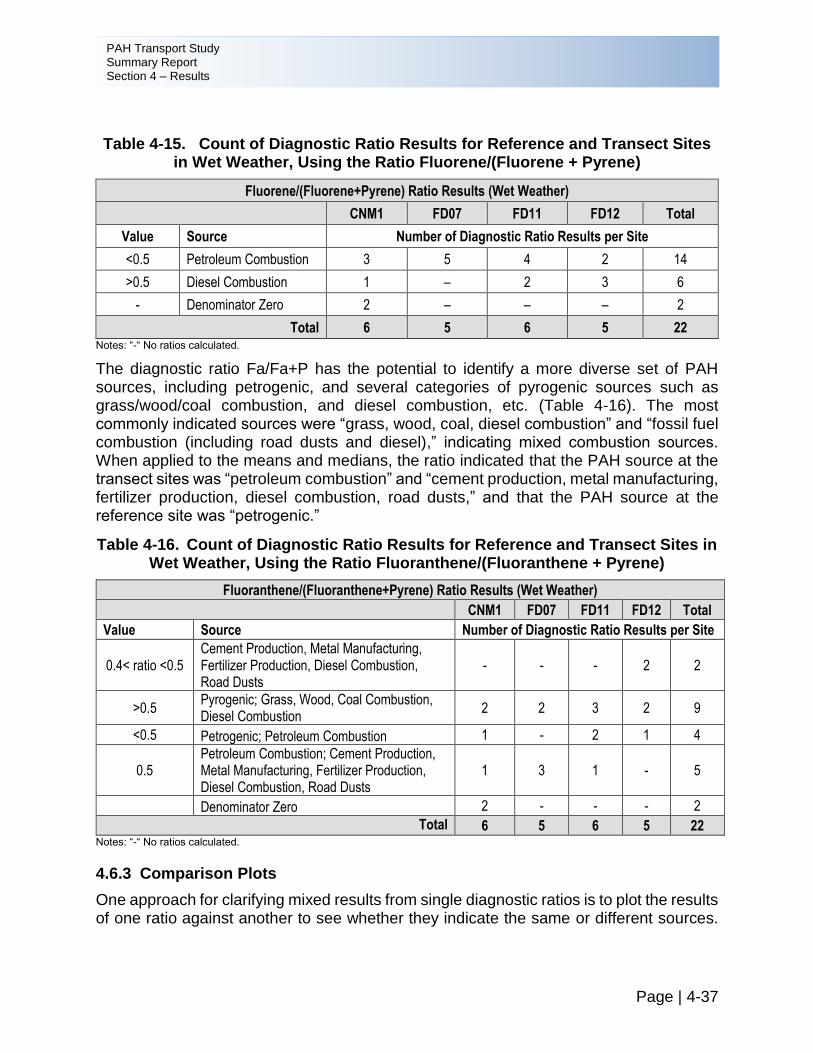
PAH Transport Study Summary Report Section 4 – Results
Page | 4-37
Table 4-15. Count of Diagnostic Ratio Results for Reference and Transect Sites in Wet Weather, Using the Ratio Fluorene/(Fluorene + Pyrene)
Fluorene/(Fluorene+Pyrene) Ratio Results (Wet Weather)
CNM1 FD07 FD11 FD12 Total
Value Source Number of Diagnostic Ratio Results per Site
<0.5 Petroleum Combustion 3 5 4 2 14
>0.5 Diesel Combustion 1 – 2 3 6
- Denominator Zero 2 – – – 2
Total 6 5 6 5 22 Notes: “-“ No ratios calculated.
The diagnostic ratio Fa/Fa+P has the potential to identify a more diverse set of PAH sources, including petrogenic, and several categories of pyrogenic sources such as grass/wood/coal combustion, and diesel combustion, etc. (Table 4-16). The most commonly indicated sources were “grass, wood, coal, diesel combustion” and “fossil fuel combustion (including road dusts and diesel),” indicating mixed combustion sources. When applied to the means and medians, the ratio indicated that the PAH source at the transect sites was “petroleum combustion” and “cement production, metal manufacturing, fertilizer production, diesel combustion, road dusts,” and that the PAH source at the reference site was “petrogenic.”
Table 4-16. Count of Diagnostic Ratio Results for Reference and Transect Sites in Wet Weather, Using the Ratio Fluoranthene/(Fluoranthene + Pyrene)
Fluoranthene/(Fluoranthene+Pyrene) Ratio Results (Wet Weather)
CNM1 FD07 FD11 FD12 Total
Value Source Number of Diagnostic Ratio Results per Site
0.4< ratio <0.5 Cement Production, Metal Manufacturing, Fertilizer Production, Diesel Combustion, Road Dusts
- - - 2 2
>0.5 Pyrogenic; Grass, Wood, Coal Combustion, Diesel Combustion
2 2 3 2 9
<0.5 Petrogenic; Petroleum Combustion 1 - 2 1 4
0.5 Petroleum Combustion; Cement Production, Metal Manufacturing, Fertilizer Production, Diesel Combustion, Road Dusts
1 3 1 - 5
Denominator Zero 2 - - - 2
Total 6 5 6 5 22 Notes: “-“ No ratios calculated.
4.6.3 Comparison Plots
One approach for clarifying mixed results from single diagnostic ratios is to plot the results of one ratio against another to see whether they indicate the same or different sources.
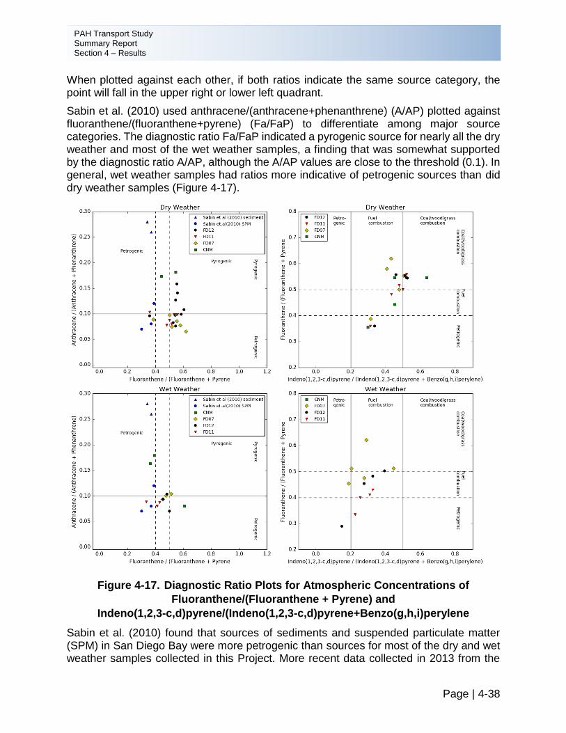
PAH Transport Study Summary Report Section 4 – Results
Page | 4-38
When plotted against each other, if both ratios indicate the same source category, the point will fall in the upper right or lower left quadrant.
Sabin et al. (2010) used anthracene/(anthracene+phenanthrene) (A/AP) plotted against fluoranthene/(fluoranthene+pyrene) (Fa/FaP) to differentiate among major source categories. The diagnostic ratio Fa/FaP indicated a pyrogenic source for nearly all the dry weather and most of the wet weather samples, a finding that was somewhat supported by the diagnostic ratio A/AP, although the A/AP values are close to the threshold (0.1). In general, wet weather samples had ratios more indicative of petrogenic sources than did dry weather samples (Figure 4-17).
Figure 4-17. Diagnostic Ratio Plots for Atmospheric Concentrations of
Fluoranthene/(Fluoranthene + Pyrene) and
Indeno(1,2,3-c,d)pyrene/(Indeno(1,2,3-c,d)pyrene+Benzo(g,h,i)perylene
Sabin et al. (2010) found that sources of sediments and suspended particulate matter (SPM) in San Diego Bay were more petrogenic than sources for most of the dry and wet weather samples collected in this Project. More recent data collected in 2013 from the
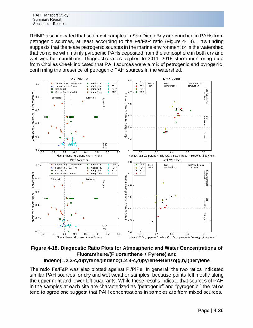
PAH Transport Study Summary Report Section 4 – Results
Page | 4-39
RHMP also indicated that sediment samples in San Diego Bay are enriched in PAHs from petrogenic sources, at least according to the Fa/FaP ratio (Figure 4-18). This finding suggests that there are petrogenic sources in the marine environment or in the watershed that combine with mainly pyrogenic PAHs deposited from the atmosphere in both dry and wet weather conditions. Diagnostic ratios applied to 2011–2016 storm monitoring data from Chollas Creek indicated that PAH sources were a mix of petrogenic and pyrogenic, confirming the presence of petrogenic PAH sources in the watershed.
Figure 4-18. Diagnostic Ratio Plots for Atmospheric and Water Concentrations of
Fluoranthene/(Fluoranthene + Pyrene) and
Indeno(1,2,3-c,d)pyrene/(Indeno(1,2,3-c,d)pyrene+Benzo(g,h,i)perylene
The ratio Fa/FaP was also plotted against Pi/PiPe. In general, the two ratios indicated similar PAH sources for dry and wet weather samples, because points fell mostly along the upper right and lower left quadrants. While these results indicate that sources of PAH in the samples at each site are characterized as “petrogenic” and “pyrogenic,” the ratios tend to agree and suggest that PAH concentrations in samples are from mixed sources.
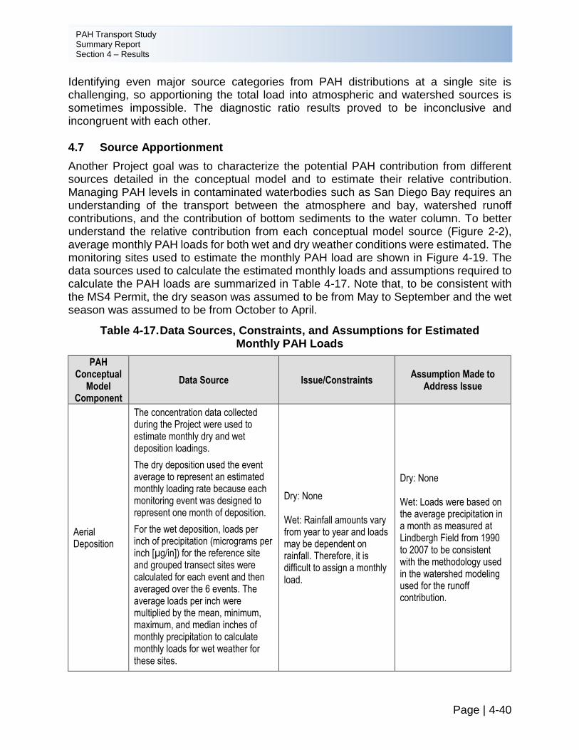
PAH Transport Study Summary Report Section 4 – Results
Page | 4-40
Identifying even major source categories from PAH distributions at a single site is challenging, so apportioning the total load into atmospheric and watershed sources is sometimes impossible. The diagnostic ratio results proved to be inconclusive and incongruent with each other.
4.7 Source Apportionment
Another Project goal was to characterize the potential PAH contribution from different sources detailed in the conceptual model and to estimate their relative contribution. Managing PAH levels in contaminated waterbodies such as San Diego Bay requires an understanding of the transport between the atmosphere and bay, watershed runoff contributions, and the contribution of bottom sediments to the water column. To better understand the relative contribution from each conceptual model source (Figure 2-2), average monthly PAH loads for both wet and dry weather conditions were estimated. The monitoring sites used to estimate the monthly PAH load are shown in Figure 4-19. The data sources used to calculate the estimated monthly loads and assumptions required to calculate the PAH loads are summarized in Table 4-17. Note that, to be consistent with the MS4 Permit, the dry season was assumed to be from May to September and the wet season was assumed to be from October to April.
Table 4-17. Data Sources, Constraints, and Assumptions for Estimated Monthly PAH Loads
PAH Conceptual
Model Component
Data Source Issue/Constraints Assumption Made to
Address Issue
Aerial Deposition
The concentration data collected during the Project were used to estimate monthly dry and wet deposition loadings.
The dry deposition used the event average to represent an estimated monthly loading rate because each monitoring event was designed to represent one month of deposition.
For the wet deposition, loads per inch of precipitation (micrograms per inch [µg/in]) for the reference site and grouped transect sites were calculated for each event and then averaged over the 6 events. The average loads per inch were multiplied by the mean, minimum, maximum, and median inches of monthly precipitation to calculate monthly loads for wet weather for these sites.
Dry: None Wet: Rainfall amounts vary from year to year and loads may be dependent on rainfall. Therefore, it is difficult to assign a monthly load.
Dry: None Wet: Loads were based on the average precipitation in a month as measured at Lindbergh Field from 1990 to 2007 to be consistent with the methodology used in the watershed modeling used for the runoff contribution.
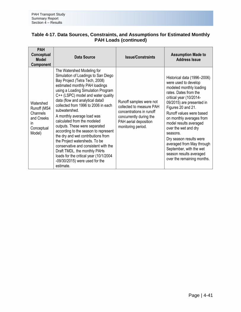
PAH Transport Study Summary Report Section 4 – Results
Table 4-17. Data Sources, Constraints, and Assumptions for Estimated Monthly PAH Loads (continued)
Page | 4-41
PAH Conceptual
Model Component
Data Source Issue/Constraints Assumption Made to
Address Issue
Watershed Runoff (MS4 Channels and Creeks in Conceptual Model)
The Watershed Modeling for Simulation of Loadings to San Diego Bay Project (Tetra Tech, 2008) estimated monthly PAH loadings using a Loading Simulation Program C++ (LSPC) model and water quality data (flow and analytical data0 collected from 1996 to 2006 in each subwatershed.
A monthly average load was calculated from the modeled outputs. These were separated according to the season to represent the dry and wet contributions from the Project watersheds. To be conservative and consistent with the Draft TMDL. the monthly PAHs loads for the critical year (10/1/2004 -09/30/2015) were used for the estimate.
Runoff samples were not collected to measure PAH concentrations in runoff concurrently during the PAH aerial deposition monitoring period.
Historical data (1996–2006) were used to develop modeled monthly loading rates. Dates from the critical year (10/2014-09/2015) are presented in Figures 20 and 21.
Runoff values were based on monthly averages from model results averaged over the wet and dry seasons.
Dry season results were averaged from May through September, with the wet season results averaged over the remaining months.
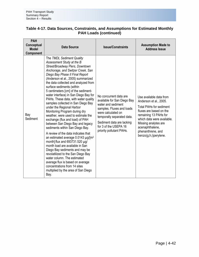
PAH Transport Study Summary Report Section 4 – Results
Table 4-17. Data Sources, Constraints, and Assumptions for Estimated Monthly PAH Loads (continued)
Page | 4-42
PAH Conceptual
Model Component
Data Source Issue/Constraints Assumption Made to
Address Issue
Bay Sediment
The TMDL Sediment Quality Assessment Study at the B Street/Broadway Piers, Downtown Anchorage, and Switzer Creek, San Diego Bay Phase II Final Report (Anderson et al., 2005) summarized the data collected and analyzed from surface sediments (within 5 centimeters [cm] of the sediment-water interface) in San Diego Bay for PAHs. These data, with water quality samples collected in San Diego Bay under the Regional Harbor Monitoring Program during dry weather, were used to estimate the exchange (flux and load) of PAH between San Diego Bay and legacy sediments within San Diego Bay.
A review of the data indicates that an estimated average 0.0143 µg/[m2 month] flux and 693731.520 µg/ month load are available in San Diego Bay sediments and may be revolatilized to the San Diego Bay water column. The estimated average flux is based on average concentrations from 14 sites multiplied by the area of San Diego Bay.
No concurrent data are available for San Diego Bay water and sediment samples. Fluxes and loads were calculated on temporally separated data.
Sediment data are lacking for 3 of the USEPA 16 priority pollutant PAHs.
Use available data from Anderson et al., 2005.
Total PAHs for sediment fluxes are based on the remaining 13 PAHs for which data were available. Missing analytes are acenaphthalene, phenanthrene, and benzo(g,h,i)perylene.
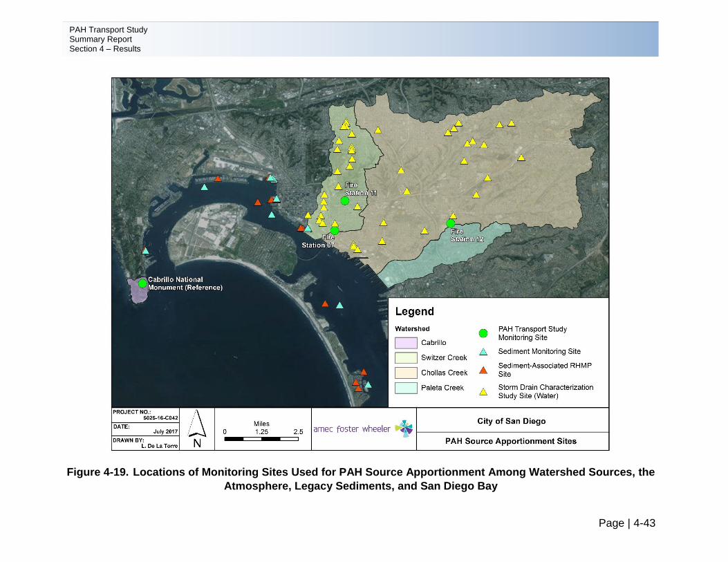
PAH Transport Study Summary Report Section 4 – Results
Page | 4-43
Figure 4-19. Locations of Monitoring Sites Used for PAH Source Apportionment Among Watershed Sources, the
Atmosphere, Legacy Sediments, and San Diego Bay

PAH Transport Study Summary Report Section 4 – Results
Page | 4-44
Intentionally Left Blank
PAH Transport Study Summary Report Section 4 – Results
Page | 4-45
Estimated monthly relative contributions from and exchange of PAHs among watershed sources, the atmosphere, and legacy sediments, during dry and wet weather, respectively, are shown in Figures 4-20 and 4-21. As noted in Table 4-17, watershed runoff and sediment sampling was not conducted concurrently with aerial deposition monitoring, therefore values from previous watershed monitoring studies were used for comparison. The values should be reviewed in that context and compared from a level of magnitude perspective.
While acknowledging the assumptions that were necessary to estimate monthly PAH loads (Table 4-17), some observations can be made. With these caveats, the calculations indicate that atmospheric deposition may be contributing substantially to San Diego Bay loads throughout the year. In dry weather conditions, dry atmospheric deposition monthly load is five to eight orders of magnitude larger watershed runoff and bay sediment leaching (Figure 4-20). The loads during the dry conditions from the reference site are two to three orders of magnitude smaller than the load from the transect sites. Although the average PAH concentrations measured in San Diego Bay waters were much lower than the average concentrations measured in the storm drain system from the City of San Diego Storm Drain Characterization Study, correspondingly low atmospheric concentrations of PAHs measured at the reference site resulted in a negative flux of gaseous phase PAHs from the atmosphere throughout the Project Area. The creeks and bay water column may be experiencing a revolatilization of PAHs into the atmosphere, based on the gas exchange calculations. In wet weather conditions as in dry weather, the load calculations show the atmosphere to be contributing PAH loads of larger than those attributed to the watershed runoff San Diego Bay (Figure 4-21). The loads during the wet conditions from the reference site are three to four orders of magnitude smaller than the load from the transect sites and of comparable magnitude to the watershed runoff.
PAH Transport Study Summary Report Section 4 – Results
Page | 4-46
Intentionally Left Blank
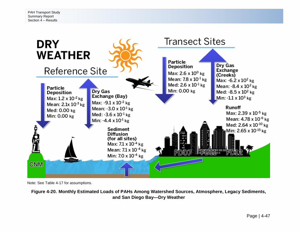
PAH Transport Study Summary Report Section 4 – Results
Page | 4-47
Note: See Table 4-17 for assumptions.
Figure 4-20. Monthly Estimated Loads of PAHs Among Watershed Sources, Atmosphere, Legacy Sediments,
and San Diego Bay—Dry Weather
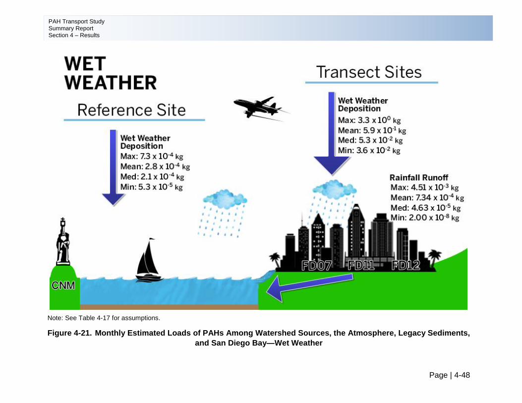
PAH Transport Study Summary Report Section 4 – Results
Page | 4-48
Note: See Table 4-17 for assumptions.
Figure 4-21. Monthly Estimated Loads of PAHs Among Watershed Sources, the Atmosphere, Legacy Sediments,
and San Diego Bay—Wet Weather
PAH Transport Study Summary Report Section 5 – Conclusions and Recommendations
Page | 5-1
5 CONCLUSIONS AND RECOMMENDATIONS
5.1 Conclusions
PAHs are continuously transported from the atmosphere into the watershed via wet weather and dry weather deposition. Controlling PAHs derived from atmospheric deposition presents a challenge for environmental managers, because the deposited PAHs may originally be from either sources outside of their jurisdiction or from local sources. Atmospheric deposition accounts for a significant portion of PAH loading to surface waters (Sabin et al., 2004).
The Project was designed to collect data needed to better understand the sources of PAHs within the San Diego urban area, relative contributions of wet versus dry deposition, and transport pathways as necessary for developing effective and defensible TMDLs or other regulatory strategies. Ultimately, this Project attempted to address two primary data gaps: (1) estimates of aerial deposition loading of PAHs to San Diego Bay and the Project watersheds; and (2) estimates of relative contributions from various sources.
To provide a better understanding of the contribution of aerially deposited PAHs to the Project watersheds, and to bridge the gap between atmospheric sources and watershed sources, a monitoring program comprising wet and dry weather components was completed during 2012-2017. The monitoring program was designed to answer a set of management questions discussed in Section 1.4. The Project was successful in answering three of the four initial questions it set out to answer.
• What are the sources of PAHs in the Project watersheds? What are the relative percentages contributed by those sources? Can they be further characterized?
Studies conducted between 2003 and 2005 by the SCCWRP and the University of California, Davis, during TMDL Phases I and II, identified the following sources of PAHs contributing to the impairment of San Diego Bay: the MS4s (City of San Diego and Caltrans), industrial facilities, airports, harbors, construction sites (regulated under Statewide Stormwater General Permits), atmospheric deposition, sediment flux, sediment resuspension, leaching from creosote pilings, ballast water, spills, and bilge water.
A literature review (City, 2012a) identified the following watershed sources as part of the project conceptual model: airport, land uses, roadways, harbor, fire, pier pilings, legacy sediment, and the atmosphere. These sources are shown in the conceptual model (Figure 2-2). To further identify the relative contributions of these sources, the Project calculated estimated PAH loadings to San Diego Bay from the major source categories, and investigated the applicability of diagnostic ratios for more refined source characterization. These analyses used both the datasets collected as part of the Project (atmosphere) and compiled under the literature review (Project watershed sediment and water datasets along with San Diego Bay sediment and water datasets).
Because the data compiled from these various sources are not coincident in time (with some data sets being collect as early as 2004), and with different
PAH Transport Study Summary Report Section 5 – Conclusions and Recommendations
Page | 5-2
experimental designs for the various programs, a number of assumptions were necessary to calculate PAH loading rates in dry and wet weather (Section 4.5).
With these caveats, the calculations indicate that atmospheric deposition may be contributing substantially to San Diego Bay loads throughout the year. In dry weather conditions, dry atmospheric deposition monthly load is five to eight orders of magnitude larger watershed runoff and bay sediment leaching (Figure 4-20). The loads during the dry conditions from the reference site are two to three orders of magnitude smaller than the load from the transect sites. In wet weather conditions as in dry weather, the load calculations show the atmosphere to be contributing PAH loads of larger than those attributed to the watershed runoff San Diego Bay (Figure 4-21). The loads during the wet conditions from the reference site are three to four orders of magnitude smaller than the load from the transect sites and of comparable magnitude to the watershed runoff.
PAH concentrations in the atmosphere may decrease through the winter months because of atmospheric scouring by rainfall, or alternatively may increase through the winter because of increased wood-burning or other heating-related combustion. Furthermore, vapor exchange of PAHs is highly dynamic, with volatilization during warmer months offsetting efficient deposition during cooler winter months (Leister and Baker, 1994).
Diagnostic ratio calculations did not provide a clear picture of the relative loadings from more specific PAH sources in the Project Area. Numerous ratios can be used to pinpoint the potential source of PAHs in the environment. Some diagnostic ratios can differentiate between gasoline and diesel fuel sources, while others are broader and can distinguish only between petrogenic and pyrogenic sources. Two diagnostic ratios were applied to the dry weather Project dataset and six diagnostic ratios were applied to the wet weather Project dataset.
The diagnostic ratio results proved to be inconclusive and incongruent with each other. This finding indicates that there are mixed sources of PAHs within the atmosphere in the Project Area. Diagnostic ratios were also applied to data gathered as part of the Project literature review. The diagnostic ratio review of the Project watershed monitoring data again indicated that PAH sources were a mix of petrogenic and pyrogenic. An assessment of the diagnostic ratios developed from data collected in the marine sediments potentially shows that the sediment in San Diego Bay may be enriched in PAHs from petrogenic sources such as unburned diesel fuel (see Section 4.6.3). In general, diagnostic ratios were not able to isolate a specific PAH source in the Project area (see Table 4-8 through Table 4-15 in Sections 4.6.1 and 4.6.2).
• What are the dry weather and wet weather deposition PAH loading rates in the Project watersheds?
Dry and wet fluxes and loads measured at urban sites were significantly higher than measured at the reference (nonurbanized) site (see Tables 5-1 through 5-3), which demonstrates that anthropogenic sources in urban areas may be
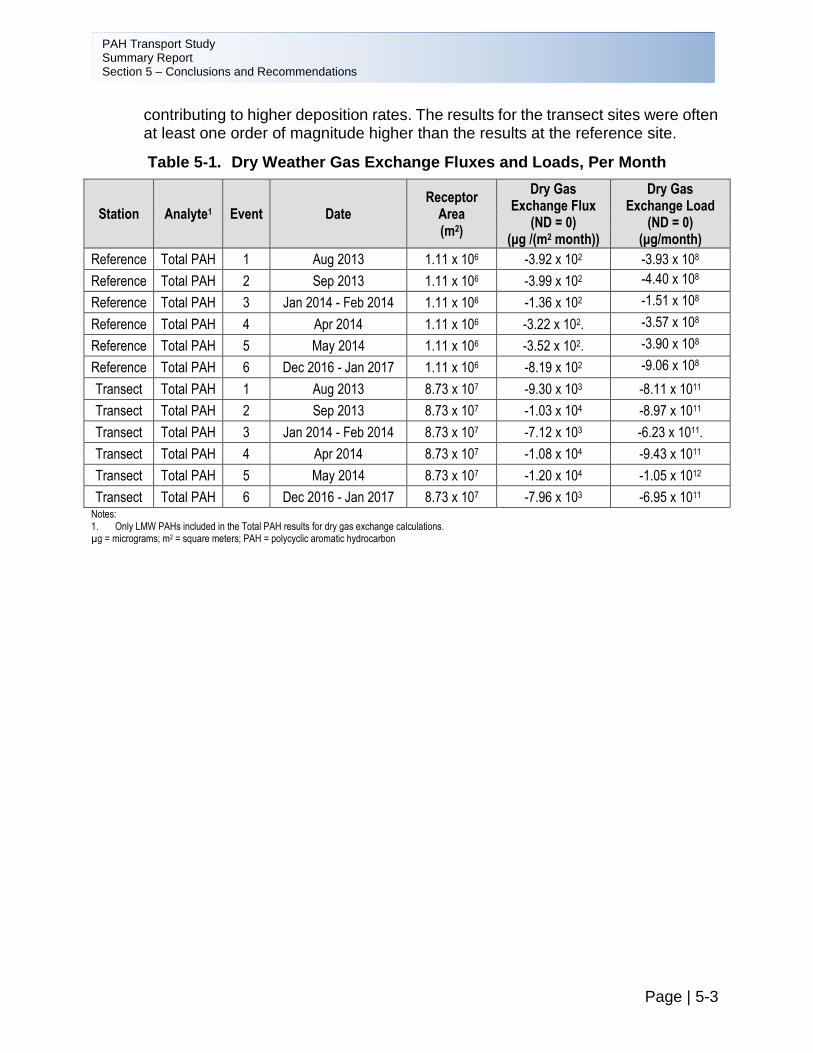
PAH Transport Study Summary Report Section 5 – Conclusions and Recommendations
Page | 5-3
contributing to higher deposition rates. The results for the transect sites were often at least one order of magnitude higher than the results at the reference site.
Table 5-1. Dry Weather Gas Exchange Fluxes and Loads, Per Month
Station Analyte1 Event Date Receptor
Area (m2)
Dry Gas Exchange Flux
(ND = 0) (μg /(m2 month))
Dry Gas Exchange Load
(ND = 0) (μg/month)
Reference Total PAH 1 Aug 2013 1.11 x 10⁶ -3.92 x 10² -3.93 x 10⁸
Reference Total PAH 2 Sep 2013 1.11 x 10⁶ -3.99 x 10² -4.40 x 10⁸
Reference Total PAH 3 Jan 2014 - Feb 2014 1.11 x 10⁶ -1.36 x 10² -1.51 x 10⁸
Reference Total PAH 4 Apr 2014 1.11 x 10⁶ -3.22 x 10². -3.57 x 10⁸
Reference Total PAH 5 May 2014 1.11 x 10⁶ -3.52 x 10². -3.90 x 10⁸
Reference Total PAH 6 Dec 2016 - Jan 2017 1.11 x 10⁶ -8.19 x 10² -9.06 x 10⁸
Transect Total PAH 1 Aug 2013 8.73 x 10⁷ -9.30 x 10³ -8.11 x 10¹¹
Transect Total PAH 2 Sep 2013 8.73 x 10⁷ -1.03 x 10⁴ -8.97 x 10¹¹
Transect Total PAH 3 Jan 2014 - Feb 2014 8.73 x 10⁷ -7.12 x 10³ -6.23 x 10¹¹.
Transect Total PAH 4 Apr 2014 8.73 x 10⁷ -1.08 x 10⁴ -9.43 x 10¹¹
Transect Total PAH 5 May 2014 8.73 x 10⁷ -1.20 x 10⁴ -1.05 x 10¹²
Transect Total PAH 6 Dec 2016 - Jan 2017 8.73 x 10⁷ -7.96 x 10³ -6.95 x 10¹¹ Notes: 1. Only LMW PAHs included in the Total PAH results for dry gas exchange calculations. µg = micrograms; m2 = square meters; PAH = polycyclic aromatic hydrocarbon
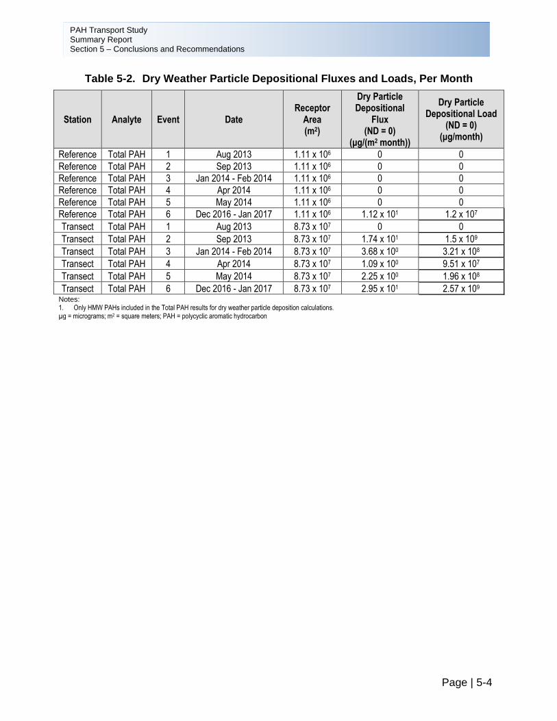
PAH Transport Study Summary Report Section 5 – Conclusions and Recommendations
Page | 5-4
Table 5-2. Dry Weather Particle Depositional Fluxes and Loads, Per Month
Station Analyte Event Date Receptor
Area (m2)
Dry Particle Depositional
Flux (ND = 0)
(μg/(m2 month))
Dry Particle Depositional Load
(ND = 0) (μg/month)
Reference Total PAH 1 Aug 2013 1.11 x 10⁶ 0 0
Reference Total PAH 2 Sep 2013 1.11 x 10⁶ 0 0
Reference Total PAH 3 Jan 2014 - Feb 2014 1.11 x 10⁶ 0 0
Reference Total PAH 4 Apr 2014 1.11 x 10⁶ 0 0
Reference Total PAH 5 May 2014 1.11 x 10⁶ 0 0
Reference Total PAH 6 Dec 2016 - Jan 2017 1.11 x 10⁶ 1.12 x 101 1.2 x 10⁷
Transect Total PAH 1 Aug 2013 8.73 x 10⁷ 0 0
Transect Total PAH 2 Sep 2013 8.73 x 10⁷ 1.74 x 101 1.5 x 10⁹
Transect Total PAH 3 Jan 2014 - Feb 2014 8.73 x 10⁷ 3.68 x 100 3.21 x 10⁸
Transect Total PAH 4 Apr 2014 8.73 x 10⁷ 1.09 x 100 9.51 x 10⁷
Transect Total PAH 5 May 2014 8.73 x 10⁷ 2.25 x 100 1.96 x 10⁸
Transect Total PAH 6 Dec 2016 - Jan 2017 8.73 x 10⁷ 2.95 x 101 2.57 x 10⁹ Notes: 1. Only HMW PAHs included in the Total PAH results for dry weather particle deposition calculations. µg = micrograms; m2 = square meters; PAH = polycyclic aromatic hydrocarbon
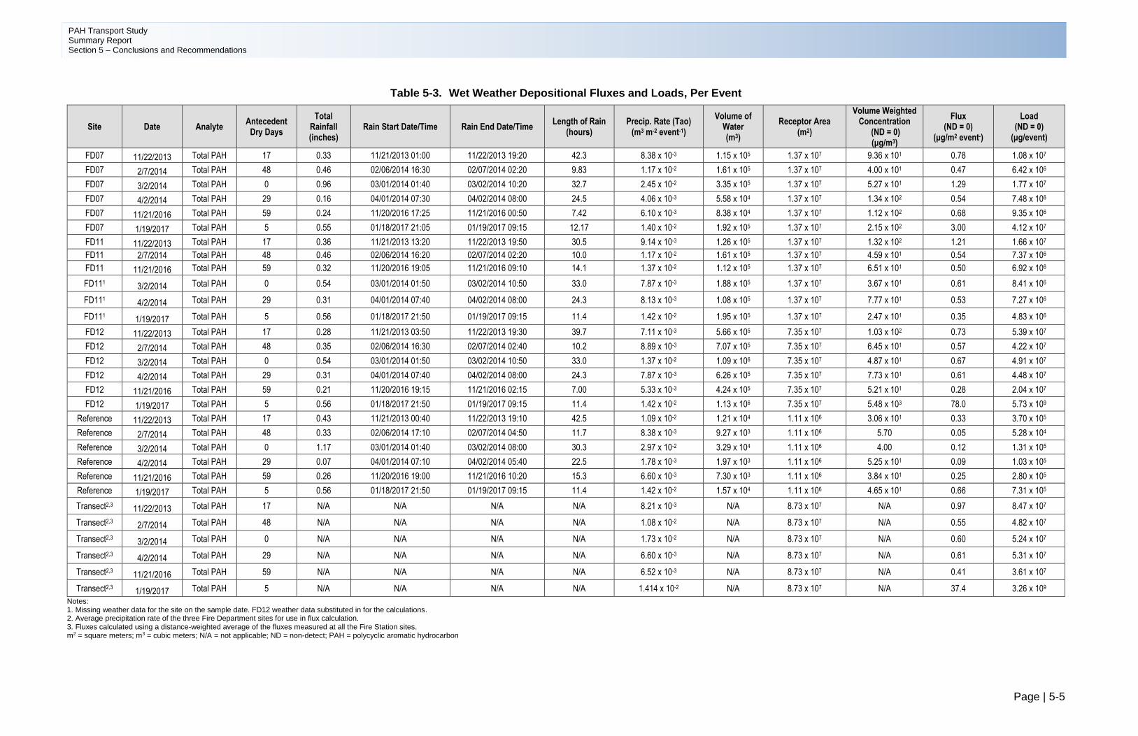
PAH Transport Study Summary Report Section 5 – Conclusions and Recommendations
Page | 5-5
Table 5-3. Wet Weather Depositional Fluxes and Loads, Per Event
Site Date Analyte Antecedent
Dry Days
Total Rainfall (inches)
Rain Start Date/Time Rain End Date/Time Length of Rain
(hours) Precip. Rate (Tao)
(m3 m-2 event-1)
Volume of Water (m3)
Receptor Area (m2)
Volume Weighted Concentration
(ND = 0) (μg/m3)
Flux (ND = 0)
(μg/m2 event-)
Load (ND = 0)
(μg/event)
FD07 11/22/2013 Total PAH 17 0.33 11/21/2013 01:00 11/22/2013 19:20 42.3 8.38 x 10⁻³ 1.15 x 10⁵ 1.37 x 10⁷ 9.36 x 101 0.78 1.08 x 10⁷
FD07 2/7/2014 Total PAH 48 0.46 02/06/2014 16:30 02/07/2014 02:20 9.83 1.17 x 10⁻² 1.61 x 10⁵ 1.37 x 10⁷ 4.00 x 101 0.47 6.42 x 10⁶
FD07 3/2/2014 Total PAH 0 0.96 03/01/2014 01:40 03/02/2014 10:20 32.7 2.45 x 10⁻² 3.35 x 10⁵ 1.37 x 10⁷ 5.27 x 101 1.29 1.77 x 10⁷
FD07 4/2/2014 Total PAH 29 0.16 04/01/2014 07:30 04/02/2014 08:00 24.5 4.06 x 10⁻³ 5.58 x 10⁴ 1.37 x 10⁷ 1.34 x 10² 0.54 7.48 x 10⁶
FD07 11/21/2016 Total PAH 59 0.24 11/20/2016 17:25 11/21/2016 00:50 7.42 6.10 x 10⁻³ 8.38 x 10⁴ 1.37 x 10⁷ 1.12 x 10² 0.68 9.35 x 10⁶
FD07 1/19/2017 Total PAH 5 0.55 01/18/2017 21:05 01/19/2017 09:15 12.17 1.40 x 10⁻² 1.92 x 10⁵ 1.37 x 10⁷ 2.15 x 10² 3.00 4.12 x 10⁷
FD11 11/22/2013 Total PAH 17 0.36 11/21/2013 13:20 11/22/2013 19:50 30.5 9.14 x 10⁻³ 1.26 x 10⁵ 1.37 x 10⁷ 1.32 x 10² 1.21 1.66 x 10⁷
FD11 2/7/2014 Total PAH 48 0.46 02/06/2014 16:20 02/07/2014 02:20 10.0 1.17 x 10⁻² 1.61 x 10⁵ 1.37 x 10⁷ 4.59 x 101 0.54 7.37 x 10⁶
FD11 11/21/2016 Total PAH 59 0.32 11/20/2016 19:05 11/21/2016 09:10 14.1 1.37 x 10⁻² 1.12 x 10⁵ 1.37 x 10⁷ 6.51 x 101 0.50 6.92 x 10⁶
FD111 3/2/2014 Total PAH 0 0.54 03/01/2014 01:50 03/02/2014 10:50 33.0 7.87 x 10⁻³ 1.88 x 10⁵ 1.37 x 10⁷ 3.67 x 101 0.61 8.41 x 10⁶
FD111 4/2/2014 Total PAH 29 0.31 04/01/2014 07:40 04/02/2014 08:00 24.3 8.13 x 10⁻³ 1.08 x 10⁵ 1.37 x 10⁷ 7.77 x 101 0.53 7.27 x 10⁶
FD111 1/19/2017 Total PAH 5 0.56 01/18/2017 21:50 01/19/2017 09:15 11.4 1.42 x 10⁻² 1.95 x 10⁵ 1.37 x 10⁷ 2.47 x 101 0.35 4.83 x 10⁶
FD12 11/22/2013 Total PAH 17 0.28 11/21/2013 03:50 11/22/2013 19:30 39.7 7.11 x 10⁻³ 5.66 x 10⁵ 7.35 x 10⁷ 1.03 x 10² 0.73 5.39 x 10⁷
FD12 2/7/2014 Total PAH 48 0.35 02/06/2014 16:30 02/07/2014 02:40 10.2 8.89 x 10⁻³ 7.07 x 10⁵ 7.35 x 10⁷ 6.45 x 101 0.57 4.22 x 10⁷
FD12 3/2/2014 Total PAH 0 0.54 03/01/2014 01:50 03/02/2014 10:50 33.0 1.37 x 10⁻² 1.09 x 10⁶ 7.35 x 10⁷ 4.87 x 101 0.67 4.91 x 10⁷
FD12 4/2/2014 Total PAH 29 0.31 04/01/2014 07:40 04/02/2014 08:00 24.3 7.87 x 10⁻³ 6.26 x 10⁵ 7.35 x 10⁷ 7.73 x 101 0.61 4.48 x 10⁷
FD12 11/21/2016 Total PAH 59 0.21 11/20/2016 19:15 11/21/2016 02:15 7.00 5.33 x 10⁻³ 4.24 x 10⁵ 7.35 x 10⁷ 5.21 x 101 0.28 2.04 x 10⁷
FD12 1/19/2017 Total PAH 5 0.56 01/18/2017 21:50 01/19/2017 09:15 11.4 1.42 x 10⁻² 1.13 x 10⁶ 7.35 x 10⁷ 5.48 x 10³ 78.0 5.73 x 10⁹
Reference 11/22/2013 Total PAH 17 0.43 11/21/2013 00:40 11/22/2013 19:10 42.5 1.09 x 10⁻² 1.21 x 10⁴ 1.11 x 10⁶ 3.06 x 101 0.33 3.70 x 10⁵
Reference 2/7/2014 Total PAH 48 0.33 02/06/2014 17:10 02/07/2014 04:50 11.7 8.38 x 10⁻³ 9.27 x 10³ 1.11 x 10⁶ 5.70 0.05 5.28 x 10⁴
Reference 3/2/2014 Total PAH 0 1.17 03/01/2014 01:40 03/02/2014 08:00 30.3 2.97 x 10⁻² 3.29 x 10⁴ 1.11 x 10⁶ 4.00 0.12 1.31 x 10⁵
Reference 4/2/2014 Total PAH 29 0.07 04/01/2014 07:10 04/02/2014 05:40 22.5 1.78 x 10⁻³ 1.97 x 10³ 1.11 x 10⁶ 5.25 x 101 0.09 1.03 x 10⁵
Reference 11/21/2016 Total PAH 59 0.26 11/20/2016 19:00 11/21/2016 10:20 15.3 6.60 x 10⁻³ 7.30 x 10³ 1.11 x 10⁶ 3.84 x 101 0.25 2.80 x 10⁵
Reference 1/19/2017 Total PAH 5 0.56 01/18/2017 21:50 01/19/2017 09:15 11.4 1.42 x 10⁻² 1.57 x 10⁴ 1.11 x 10⁶ 4.65 x 101 0.66 7.31 x 10⁵
Transect2,3 11/22/2013 Total PAH 17 N/A N/A N/A N/A 8.21 x 10⁻³ N/A 8.73 x 10⁷ N/A 0.97 8.47 x 10⁷
Transect2,3 2/7/2014 Total PAH 48 N/A N/A N/A N/A 1.08 x 10⁻² N/A 8.73 x 10⁷ N/A 0.55 4.82 x 10⁷
Transect2,3 3/2/2014 Total PAH 0 N/A N/A N/A N/A 1.73 x 10⁻² N/A 8.73 x 10⁷ N/A 0.60 5.24 x 10⁷
Transect2,3 4/2/2014 Total PAH 29 N/A N/A N/A N/A 6.60 x 10⁻³ N/A 8.73 x 10⁷ N/A 0.61 5.31 x 10⁷
Transect2,3 11/21/2016 Total PAH 59 N/A N/A N/A N/A 6.52 x 10⁻³ N/A 8.73 x 10⁷ N/A 0.41 3.61 x 10⁷
Transect2,3 1/19/2017 Total PAH 5 N/A N/A N/A N/A 1.414 x 10⁻² N/A 8.73 x 10⁷ N/A 37.4 3.26 x 10⁹
Notes: 1. Missing weather data for the site on the sample date. FD12 weather data substituted in for the calculations. 2. Average precipitation rate of the three Fire Department sites for use in flux calculation. 3. Fluxes calculated using a distance-weighted average of the fluxes measured at all the Fire Station sites. m2 = square meters; m3 = cubic meters; N/A = not applicable; ND = non-detect; PAH = polycyclic aromatic hydrocarbon

PAH Transport Study Summary Report Section 5 – Conclusions and Recommendations
Page | 5-6
Intentionally Left Blank
PAH Transport Study Summary Report Section 5 – Conclusions and Recommendations
Page | 5-7
• How can the collected data on aerially deposited PAHs be used to aid TMDL development or guide future management efforts?
The Project provided a greater understanding of atmospheric deposition fluxes and loads of PAHs to San Diego Bay and its urbanized watershed. The results provide context for the relative contribution of the different sources of PAHs in the Project watersheds, including the relative contributions from atmospheric versus other sources in wet weather versus dry weather. The data collected as part of this Project filled some data gaps outlined in the Project conceptual model. This information may help allocate TMDL loads. Depending on the needs of future regulatory actions, the aerial PAH concentrations measured as part of this Project can be input into a holistic model of PAH transport in the Project Area.
5.2 Recommendations
Potential next steps to address the remaining data gaps and the unanswered Project management question are summarized as follows:
• What are the next steps required to characterize aerial PAH sources for TMDL implementation? What type of environmental monitoring would be needed and what would be most effective?
o Data collected under this Project have addressed some data gaps. However, additional data collection or resolution in data may be advised to further the understanding of PAHs in the atmosphere and their sources. Additional study options include the following:
▪ To better quantify the dry weather particle deposition and vapor flux, sample collection and analysis may use a modified method to analyze the gas and particle phases separately. However, because the watershed and sediment loads estimated are so much larger than dry weather atmospheric loads, this determination may not be needed.
▪ Concurrent wet weather deposition samples and stream water/discharge samples could be collected and analyzed to better compare PAH atmospheric deposition and watershed loading to San Diego Bay.
▪ Because diagnostic ratios in the Project were inconclusive, to achieve better resolution, point source monitoring stations (rather than ambient transect sites) may be installed to determine the signal from known emission sources within the Project watershed. These data could be used for fingerprinting or other source identification methods and could potentially determine the relative contributions from more specific sources.
The data collected as part of this Project may be considered in the development of pending TMDLs or other appropriate regulatory actions. The findings of the Project should be considered during the development of these regulatory actions, especially the finding that PAHs from the atmosphere may be a principal factor in wet weather PAH loads. The wet weather contributions are orders of magnitude higher than dry weather loading
PAH Transport Study Summary Report Section 5 – Conclusions and Recommendations
Page | 5-8
contributions. It is recommended that the City coordinate with the San Diego Air Pollution Control District during the development of the regulatory action, because atmospheric sources and loads are outside the control of the City.
Additionally, it will be determined whether modeling is a necessary component of the regulatory action. If modeling is implemented, data from this Project can assist in calibration and validation of the model.
PAH Transport Study Summary Report Section 6 – References
Page | 6-1
6 REFERENCES
Abdel-Shafy, H.I. and M.S. Mansour. 2016. A review on polycyclic aromatic
hydrocarbons: Source, environmental impact, effect on human health and
remediation. Egyptian Journal of Petroleum. Volume 25, Issue 1, March 2016,
Pages 107-123. https://doi.org/10.1016/j.ejpe.2015.03.011.
Air Toxics Ltd. (Air Toxics). 2012. Sorbent & Solution Sampling Guide.
Anderson et al. 2005. TMDL Sediment Quality Assessment Study at the B
Street/Broadway Piers, Downtown Anchorage, and Switzer Creek, San Diego.
Phase II. Final Report. Temporal Variability, Causes of Impacts, And Likely
Sources of Contaminants of Concern. June 2005.
Andersson, J.T. and C. Achten. 2015. Time to Say Goodbye to the 16 EPA PAHs?
Toward an Up-to-Date Use of PACs for Environmental Purposes. Polycycl.
Aromat. Compd. 35, 330–354. doi:10.1080/10406638.2014.991042.
ASTM D6209-13, Standard Test Method for Determination of Gaseous and Particulate
Polycyclic Aromatic Hydrocarbons in Ambient Air (Collection on Sorbent-Backed
Filters with Gas Chromatographic/Mass Spectrometric Analysis), ASTM
International, West Conshohocken, PA, 2013, www.astm.org
California Regional Water Quality Control Board. San Diego Region. (San Diego Water
Board). 2013. Total Maximum Daily Loads for Toxic Pollutants in Sediment at San
Diego Bay Shorelines – Mouths of Paleta, Chollas, and Switzer Creeks. Draft
Technical Report. June 5, 2013. http://www.waterboards.ca.gov/sandiego.
City. 2007. City of San Diego Aerial Deposition Study. Final Report. Submitted to City of
San Diego. Submitted by Weston Solutions, Inc. Carlsbad, California.
September 4, 2007.
City. 2009a. City of San Diego Aerial Deposition Study, Phase III. Source Evaluation of
TMDL Metals in Chollas Creek Watershed. Final Report. Submitted to City of San
Diego. Submitted by:Weston Solutions, Inc. Carlsbad, California. June 17, 2009.
City. 2009b. City of San Diego Aerial Deposition Study, Phase II. Final Report. Submitted
to City of San Diego. Submitted by: Weston Solutions, Inc. Carlsbad, California.
March 23, 2009.
PAH Transport Study Summary Report Section 6 – References
Page | 6-2
City. 2012a. PAH Source Tracking Study Development Technical Memorandum.
Submitted to City of San Diego Transportation and Stormwater Department.
Submitted by AMEC Environment & Infrastructure, Inc. b San Diego, California.
June 2012. AMEC Project No. 5013110026.
City. 2012b. Site Selection Guidance. Technical Memorandum. Submitted to City of San
Diego Transportation and Stormwater Department. Submitted by AMEC
Environment & Infrastructure, Inc. San Diego, California. September 2012. AMEC
Project No. 5025121032.
City. 2013. PAH Transport Study-Phase II. Monitoring Plan. Submitted to City of San
Diego Transportation and Stormwater Department. Submitted by AMEC
Environment & Infrastructure, Inc. San Diego, California. April 2013. AMEC Project
No. 5025121032.
City. 2016. Polycyclic Aromatic Hydrocarbon (PAH) Transport Study. Quality Assurance
Project Plan. June 2016. Prepared for City of San Diego Transportation and
Stormwater Department. Prepared by Amec Foster Wheeler Environment &
Infrastructure, Inc. San Diego, CA.
Datta, A.K. 2002. Biological and bioenvironmental heat and mass transfer. New York:
Marcel Dekker.
Desert Research Institute (DRI). 2012. Wind Direction.
http://www.wrcc.dri.edu/htmlfiles/westwinddir.html
Electric Power Research Institute (EPRI). 2000. Literature review of background
polycyclic aromatic hydrocarbons. Final report; March 2000.
European Commission. 2001. Ambient air pollution by Polycyclic Aromatic Hydrocarbons
(PAH). Position Paper. ISBN 92-894-2057-X.
Irwin, R.J. 1997. Environmental Contaminants Encyclopedia. Fluorene Entry. National
Park Service. Water Resources Divisions, Port Collins, Colorado.
Lavin, K.S., K.J. Hageman, S.K. Marx, P.W. Dillingham, and B.S. Kamber. 2011. Using
Trace Elements in Particulate Matter to Identify the Sources of Semivolatile
Organic Contaminants in Air at an Alpine Site. Environmental Science and
Technology X: A-I.
b AMEC Environment & Infrastructure, Inc. (AMEC) is now known as Amec Foster Wheeler Environment & Infrastructure, Inc. (Amec Foster Wheeler).
PAH Transport Study Summary Report Section 6 – References
Page | 6-3
Lee, D. and K.W. Nicholson. 1994. The Measurement of Atmospheric Concentrations and
Deposition of Semi-Volatile Organic Compounds. Environmental Monitoring and
Assessment. 32: 59-91.
Leister, D. and J. Baker. 1994. Atmospheric Deposition of Organic Contaminants to the
Chesapeake Bay. Atmospheric Environment, Volume 28, Issue 8, p. 1499-1520.
Maliszewska-Kordybach, B. 1999. Sources, Concentrations, Fate and Effects of
Polycyclic Aromatic Hydrocarbons (PAHs) in the Environment. Part A: PAHs in Air.
Polish Journal of Environmental Studies 8: 131-136.
Maryland Department of Natural Resources. 2017. Atmospheric Deposition.
http://dnr.maryland.gov/streams/Pages/atmosphericdeposition.aspx. Accessed
September 2017.
National Atmospheric Deposition Program (NADP). 2011. Instruction Manual NADP/NTN
Site Selection and Installation Revised 2011-05 Version 1.5.
National Weather Service (NWS). 2012. http://www.wrh.noaa.gov/sgx/media/
media.php?wfo=sgx.
Opuene, K., O.O. Adegboro., and I.E. Agbozu. 2009. A critical appraisal of PAH indices
as indicators of PAH source and composition in Elelenwo Creek, southern Nigeria.
Environmentalist 29, 47–55. doi:10.1007/s10669-008-9181-5.
Park, S.-U., J.-G. Kim, M.-J.Jeong, and M.-J. Song. 2011. Source Identification of
Atmospheric Polycyclic Aromatic Hydrocarbons in Industrial Complex Using
Diagnostic Ratios and Multivariate Factor Analysis. Archives of Environmental
Contamination and Toxicology 60: 576-589.
Ray, S., P.S. Khillare, T. Agrarwal, and V. Shridhar. 2008. Assessment of PAHs in soil
around the International Airport in Delhi, India. Journal of Hazardous Materials 156:
9-16.
Rhea, D. et al. 2005. Polycyclic Aromatic Hydrocarbons in Water, Sediment, and Snow,
From Lakes in Grand Teton National Park, Wyoming. Final Report, USGS-CERC-
91344. February 2005.
Sabin, L.D, K.C. Schiff, J.H. Lim., and K.D. Stolzenbach., 2004. Atmospheric
concentrations of PAH, pesticides, and other semi-volatile organic compounds in
the Los Angeles coastal region. Atmospheric Pesticides. 61-72.
PAH Transport Study Summary Report Section 6 – References
Page | 6-4
Sabin, L.D., K.A. Maruya, L.A.O. Wenjian, D. Diehl, D. Tsukada, K.D. Stolzenbach., K.C.
Schiff. 2010. Exchange of polycyclic aromatic hydrocarbons among the
atmosphere, water, and sediment in coastal embayments of Southern California,
USA. Environ. Toxicol. Chem. 29, 265–274. doi:10.1002/etc.54.
Pederson, J. 2006.Essential Concepts in Atmospheric Deposition. Presented on behalf
of the State Air Resources Board, State Water Quality Control Board, and the
California Environmental Protection Agency. February 9, 2006.
http://www.waterboards.ca.gov/water_issues/hot_topics/atmospheric/presentatio
ns/jim_pederson.pdf.
Stolzenbach, K.D. 2006. Atmospheric Deposition. Southern California Report Card 2006.
UCLA Institute of the Environment.
Stogiannidis, E. and R. Laane. 2015. Source Characterization Of Polycyclic Aromatic
Hydrocarbons By Using Their Molecular Indices: An Overview Of Possibilities. Rev
Environ Contam Toxicol. 2015;234:49-133. doi: 10.1007/978-3-319-10638-0_2.
Stout, S.A., 2015. Beyond 16 Priority Pollutant PAHs: A Review of PACs used in
Environmental Forensic Chemistry. Polycycl. Aromat. Compd. 35.
Tetra Tech, 2008. Watershed Modeling for Simulation of Loadings to San Diego Bay.
Final. Prepared for: U.S. Environmental Protection Agency, Region 9. San Diego
Regional Water Quality Control Board. March 25, 2011.
Tisch Environmental. 2012. Products-TE-1000, PUF Polyurethane Foam Sampler in
Ambient Air and Pesticide Sampler. http://tisch-env.com/products/15-VOC-Ambient-
Monitors-Active-and-Passive/33-TE-1000/
Tobiszewski, M. 2014. Application of Diagnostic Ratios of PAHs to Characterize the
Pollution Emission Sources. 5th International Conference on Environmental
Science and Technology IPCBEE vol.69 (2014) © (2014) IACSIT Press, Singapore
DOI: 10.7763/IPCBEE. 2014. V69. 9.
Tobiszewski, M. and J. Namieśnik. 2012. PAH diagnostic ratios for the identification of
pollution emission sources. Environ. Pollut. 162, 110–119.
doi:10.1016/j.envpol.2011.10.025.
Tran, K., C.C. Yu, and E.Y. Zeng. 1996. Petrogenic and Biogenic Sources of N-Alkanes
off San Diego, California. Southern California Coastal Water Research Project.
Annual Report 1994-1995: 53-62.
PAH Transport Study Summary Report Section 6 – References
Page | 6-5
United States Environmental Protection Agency (USEPA). 1983. Technical Assistance
Document for Sampling and Analysis of Toxic Organic Compounds in Ambient Air.
EPA Environmental Monitoring Systems Laboratory. June 1983. EPA-600/4-83-
027.
USEPA. 1999. Compendium of Methods for the Determination of Toxic Organic
Compounds, Second Edition. Compendium Method TO-13A. Determination of
Polycyclic Aromatic Hydrocarbons (PAHs) in Ambient Air Using Gas
Chromatography/Mass Spectrometry (GC/MS). January 1999. EPA Center for
Environmental Research Information. EPA/625/R-96/010b.
USEPA. 2001. Frequently Asked Questions about Atmospheric Deposition. A Handbook
for Watershed Managers. Office of Wetlands, Oceans, and Watersheds. U.S.
Environmental Protection Agency.
http://www.epa.gov/oaqps001/gr8water/handbook/airdep_sept.pdf.
USEPA. 2008. QA Handbook for Air Pollution Measurement Systems, Volume II, Ambient
Air Quality Monitoring Program. EPA-454/B-08-003.
PAH Transport Study Summary Report Section 6 – References
Page | 6-6
Intentionally Left Blank
PAH Transport Study Summary Report Appendices
Appendix A Quality Assurance Project Plan

PAH Transport Study Summary Report Appendices
Intentionally Left Blank
PAH Transport Study Summary Report Appendices
Appendix B Data Quality Objectives and Quality Assurance and
Quality Control Review
PAH Transport Study Summary Report Appendices
Intentionally Left Blank
PAH Transport Study Summary Report Appendices
Appendix C Laboratory Reports and EDDs (electronic submittal
only)

PAH Transport Study Summary Report Appendices
Intentionally Left Blank
PAH Transport Study Summary Report Appendices
Appendix D Summary Statistics

PAH Transport Study Summary Report Appendices
Intentionally Left Blank

PAH Transport Study Summary Report Appendices
Appendix E Diagnostics Ratios from Literature Review

PAH Transport Study Summary Report Appendices
Intentionally Left Blank


