Polydispersed flow modelling using population balances in an adaptive mesh finiteelement framework

Gaurav Bhutania,b,∗, Pablo R. Brito-Paradaa,b, Jan J. Cilliersa

aRio Tinto Centre for Advanced Mineral Recovery, Department of Earth Science and Engineering, Imperial College London, South Kensington Campus, LondonSW7 2AZ, United Kingdom

bApplied Modelling and Computation Group, Department of Earth Science and Engineering, Imperial College London, South Kensington Campus, London SW72AZ, United Kingdom

Abstract

An open-source finite element framework to model multiphase polydispersed flows is presented in this work. The Eulerian–Eulerianmethod was coupled to a population balance equation and solved using a highly-parallelised finite element code—Fluidity. Thepopulation balance equation was solved using DQMOM. A hybrid finite element–control volume method for solving the coupledsystem of equations was established. To enhance the efficiency of this solver, fully-unstructured non-homogeneous anisotropicmesh adaptivity was applied to systematically adapt the mesh based on the underlying physics of the problem. This is the first timemesh adaptivity has been applied to the external coordinates of the population balance equation for modelling polydispersed flows.Rigorous model verification and benchmarking were also performed to demonstrate the accuracy of this implementation. This finiteelement framework provides an efficient alternative to model polydispersed flow problems over the other available finite volumeCFD packages.

Keywords: Polydispersed flow, Population balance modeling, DQMOM, Multiphase flow, Finite element method, Meshadaptivity

1. Introduction

Multiphase polydispersed flows are essential elements of thechemical process industry and are found extensively in pharma-ceutical, minerals processing and food processing operations,to name a few. Some of the applications where polydispersityplays a prominent role are fluidised beds, chemical reactors,bubble columns, and the spray of fuels in automotive and air-craft engines (Marchisio and Fox, 2013). A good understandingand prediction of these flows is therefore crucial for the opti-mum design of chemical process systems.

The term polydispersity refers to the heterogeneity of the dis-persed particles, which may exist due to the variation in particlesize or any other particle property in space. Developing and per-forming experiments for the applications involving multiphasepolydispersed flows is extremely challenging and becomes ex-pensive when one is interested in exploring different operatingconditions and designs. Computational Fluid Dynamics (CFD)on the other hand provides a cost effective tool to carry out theaforementioned tasks and study scale-up. Until a few decadesago it was extremely challenging to model complex industrialflow systems, but with the advent of parallelised machines andimproved algorithms it has become possible to approach theseproblems computationally.

∗Corresponding authorEmail addresses: g.bhutani12@imperial.ac.uk (Gaurav Bhutani),

pbritopa@imperial.ac.uk (Pablo R. Brito-Parada),j.j.cilliers@imperial.ac.uk (Jan J. Cilliers)

Even though the computational power and techniques have ad-vanced tremendously over the past few years, chemical engi-neers interested in modelling polydispersed flows are still con-strained by the available (commercial and non-commercial)CFD software products. There are not many options avail-able when it comes to modelling polydispersed flows and theones available do not utilise the mathematical resources ef-ficiently, and hence are sub-optimal. This paper introducesa computationally-efficient, open-source, Finite Element (FE)framework to model polydispersed flows using parallelisedadaptive mesh refinement.

Dispersed particles are commonly modelled using two differentapproaches—the Lagrangian way and the Eulerian way. Thecontinuous phase, on the other hand, is treated as a continuumin most approaches and is therefore modelled using the Eule-rian method. This leads to the popular Eulerian–Lagrangian andthe Eulerian–Eulerian methods for simulating multiphase flows(Prosperetti and Tryggvason, 2007). The Eulerian–Lagrangianmethod can become prohibitively expensive when the numberof dispersed particles is large and due to this reason the litera-ture on polydispersed flow modelling in chemical engineeringresearch has been dominated by the Eulerian–Eulerian methodin the past few years.

Multiphase Eulerian–Eulerian flow equations coupled to a Pop-ulation Balance Equation (PBE) have been used by many tomodel polydispersed flow systems in the last decade (Chenet al., 2004; Bannari et al., 2008; Buffo et al., 2012). PBE,

Preprint submitted to Computers and Chemical Engineering January 14, 2016

which is a conservation equation for the dispersed particles,is used to model the evolution of the particle size distribution(Ramkrishna, 2000). Although different methods have beenproposed to solve the PBE, one method that has attracted spe-cial attention from the research community is the method ofmoments (Frenklach and Harris, 1987), particularly for poly-dispersed flow modelling where the PBE is coupled to theEulerian–Eulerian multiphase flow equations. Method of mo-ments encapsulates a general family of methods depending thetype of closure used to close the approximated moment set.Two of the popular methods of this type are the QuadratureMethod of Moments (QMOM) (McGraw, 1997) and the Di-rect Quadrature Method of Moments (DQMOM) (Marchisioand Fox, 2005).

Zucca et al. (2006) successfully demonstrated the couplingof DQMOM to the flow equations in solving a polydispersedflow problem. DQMOM provides an efficient closure and ismore economical when compared to the other methods to solvePBEs. Marchisio and Fox (2005) showed that the PBE canbe approximated to a good accuracy by as few as four mo-ment equations in DQMOM. This is a very small number ofequations when compared to the method of classes—the othermethod used to solve PBEs (Marchal et al., 1988; Sanyal et al.,2005; Bannari et al., 2008). This particular advantage overother PBE solution methods, along with its adaptive quadra-ture approach, has inspired many researchers to use DQMOMto model polydispersed flows lately (Zucca et al., 2006; Selmaet al., 2010; Chan et al., 2010).

However, most implementations of the models to solve poly-dispersed flows have been in the following software pack-ages:

1. OpenFOAM R© (an open-source finite volume software):Silva and Lage (2011); Selma et al. (2010); Becker et al.(2014); Favero et al. (2015).

2. ANSYS R© Fluent R© (a commercial finite volume software):Zucca et al. (2006); Buffo et al. (2012); Szilagyi et al.(2014).

3. ANSYS R© CFX R© (a commercial control volume finite ele-ment software): Silva et al. (2008); Yeoh et al. (2012).

Engineers, in some sense, have been limited by the use of thesesolvers when modelling polydispersed flows and there has notbeen much discussion in the literature to improve their effi-ciency. In fact, having an efficient solver is as important ashaving a good model because a non-optimal solver can some-times force the engineer to revert to a crude model to make ittractable for solving industrial design problems. There havebeen some efforts recently to use novel computational tech-niques for solving the population balance equation (Prakashet al., 2013; Santos et al., 2013), yet there does not exist anefficient framework that can handle an industrial-scale hetero-geneous problem. In order to address this issue, DQMOM wasimplemented in a finite element framework in this work andwas coupled to the Eulerian–Eulerian method to solve multi-phase polydispersed flow problems. All equations were solved

using the open-source multiphase CFD code—Fluidity, whichsolves the Navier–Stokes and accompanying field equations onunstructured meshes using the finite element method (AMCG,2015). This framework not only provides a new open-source al-ternative to the available software packages for solving polydis-persed flow equations, but it also provides the features of the fi-nite element method—like higher order discontinuous Galerkinand continuous Galerkin methods—compared to the other soft-ware packages employing the finite volume/ control volumemethods.

Most CFD packages solve the flow equations on fixed meshesthat do not change as the simulation progresses. These meshesmay allow for anisotropy and/or inhomogeneity based on theinitial condition or a general understanding of the flow physics(e.g. boundary layer flow) but are rarely optimum for a tran-sient CFD problem. In reality, almost every transient simu-lation involves one or more time evolving phenomena, whichdrive the varying spatial requirement for the optimal place-ment of the mesh nodes. Therefore, to enhance the efficiencyof the solution method in this work, fully unstructured, non-homogeneous, anisotropic mesh adaptivity was applied in a par-allelised environment to systematically adapt the mesh based onthe underlying physics of the problem (Piggott et al., 2009). Im-proved solution efficiency through optimised adaptive mesheswill make it possible to compute large-scale flows in a tractablemanner. To the best of the authors’ knowledge, this is the firsttime adaptive mesh refinement has been applied to the externalcoordinates of the population balance equation for modellingpolydispersed flows.

The remaining part of this paper is organised as follows. Sec-tion 2 describes the model that was used to solve the polydis-persed flow problem. It starts with a discussion on the formula-tion of the flow equations and the population balance equation,followed by a brief explanation of the finite element implemen-tation of the coupled system and the solution algorithm. Thesection closes with a discussion of the mesh adaptivity tech-nique that was utilised to improve the efficiency of the solu-tion method in this paper. Section 3 shows model verifica-tion results for the DQMOM implemention described in thiswork. The polydispersed flow problem that was solved andthe corresponding results are presented in Section 4; results fora monodispersed case are presented first, followed by a fullypolydispersed flow problem. The improvements achieved bythe use of mesh adaptivity are also quantified and discussedin this section. Finally, the conclusions of this work are sum-marised in Section 5.

2. Model description and solution

2.1. Flow equations

In general, polydispersed flows consist of one continuous phaseand one (or more) dispersed phase(s). For simplicity of discus-sion, a problem consisting of one dispersed and one continuousphase was solved on a 2D domain in this work, although all

2

methods were implemented to be able to handle multiple dis-persed phases in up to three spatial dimensions.

Interpenetrating multiphase flows are generally modelled us-ing three different approaches depending on the flow regime,problem complexity and the availability of computational re-sources. The simplest technique is the mixture model whereonly one momentum equation is solved for an average mixturephase (Bowen, 1976). All other phase relative velocities arecomputed from an empirical or an analytical equation. For thisreason, the mixture model is not able to predict the dispersedphase velocity field accurately. A better but more complexmodel is the Eulerian–Eulerian multiphase model, where a sep-arate momentum equation for each phase is solved. All phasesin this method are assumed to be continuous and a model forthe interphase force terms, which couple the momentum equa-tions between any two phases, is needed. The third, and themost expensive, model is the Eulerian–Lagrangian model. Asthe name suggests, all dispersed particles are modelled as dis-crete objects with an Eulerian flow model for the continuousphase. This approach can become prohibitively expensive whenthe number of particles is large.

Considering the limitations of the mixture model and theEulerian–Lagrangian model, an incompressible multiphaseEulerian–Eulerian method was chosen to model the two phasesin this work. This method offered a practical approach tomodel polydispersed flows over the other aforementioned tech-niques.

In the Eulerian–Eulerian method, a volume-averaged momen-tum equation is derived for each phase over volumes of ap-propriate sizes (Brennen, 2005). These representative volumesshould be large enough to contain several dispersed particlesand small enough for the gradients of the volume-averaged flowproperties to remain continuous. This volume averaging givesrise to a conserved scalar called volume fraction and the mo-mentum equation for phase i, in terms of this volume fraction,is given as (Brennen, 2005):

αiρi∂ui

∂t+ αiρiui · ∇ui = −αi∇p + αiρig + ∇ · (αiτi) + fi, (1)

where the phase i can be continuous or dispersed, given in thistext by c and d respectively. αi is the volume fraction of phasei, ρi is the phase density, ui is the phase velocity, p is the staticpressure, g is the acceleration due to gravity, τi is the devia-toric stress tensor, and fi is the interphase force term. Note thatEinstein’s notation is not used in Equation (1).

The phases in Equation (1) were modelled as interpenetratingcontinua with each phase having its own velocity field so thatmixing could be modelled effectively. There was a commonpressure field considered for all the phases, as can be seenfrom Equation (1). This approximation is reasonable in situ-ations where the relative velocity between the phases is smalland the change in dispersed phase volume is negligible (Yeohet al., 2013). Separate pressure fields for the two phases may beneeded in the case of the above conditions not being satisfied.The common pressure field approximation simplified the flow

equations as only one continuity equation had to be satisfied forall phases. The combined continuity equation that was solvedin this work is given by (Brennen, 2005):

Nphases∑i=1

∇ · (αiui) = 0. (2)

The viscous stress term in Equation (1) was modelled as

∇ · (αiτi) = ∇ · (αiµi∇ui), (3)

as described in Jacobs et al. (2013), where µi is the dynamic vis-cosity of phase i. The momentum equations for the two phasesand the combined continuity equation, Equations (1) and (2) re-spectively, were solved in conjunction with the following twoequations for the volume fractions, to get the complete set offlow variables:

∂αd

∂t+ ∇ · (αdud) = 0, (4)

which was solved to get the dispersed phase volume fraction αd

and the conservation equation

Nphases∑i=1

αi = 1, (5)

which was used to obtain continuous phase volume fraction αc.No turbulence model was solved in this work as all flow condi-tions were laminar.

In polydispersed flow modelling, the most important term in themomentum equation is the interphase force fi. This includesforces such as drag, lift and the virtual mass force acting onphase i from all other phases. In the present work, only thecontribution from the drag force was considered for the inter-phase force term and the other two forces were neglected, sameas Chen et al. (2004). The interphase drag force can be writtenas:

f D =3αcαdCDρc(uc − ud)|uc − ud |

4d, (6)

where CD is the drag coefficient and d is the dispesed phase di-ameter. The popularly used Schiller–Naumann drag coefficient(Schiller and Naumann, 1935) was selected for this work. It isgiven as:

CD =

24Red

(1 + 0.15Red

0.687)

if Red < 1000,

0.44 otherwise,(7)

where Red, the dispersed phase (or particle) Reynolds number,is defined as:

Red =ρcd|uc − ud |

µc. (8)

The interphase drag force can have a strong dependence on thedispersed phase diameter d (Tabib et al., 2008), and choosing acorrect value for d becomes essential when solving a polydis-persed flow system. In many works, the value of d, obtained

3

from experiments, has been considered constant over the wholedomain for simplicity (McClure et al., 2014). Polydispersedflows on the other hand, by definition, have a dispersed phasewhose size varies over space and time, and this variation can besignificant in many cases. For this reason, a population balanceequation was solved to accurately model the polydispersity ofthe flow, which is discussed next.

2.2. Population balance equation

The Population Balance Equation (PBE) is simply a conser-vation equation for the number of dispersed particles, whichis used to model the evolution of the particle size distribution(Ramkrishna, 2000). As discussed previously, the need for apopulation balance equation arises for the prediction of particlesize distribution to accurately model the drag force term in mo-mentum equations (Equation (1)). Additionally, it may also beimportant to have some knowledge of the distribution of particlesizes in the domain for a general understanding of the flow phe-nomenon. It must be noted that ‘particle size’ and ‘dispersedphase size’ have been, and will be, used interchangeably andthey mean the same thing in the context of this work.

The particle size distribution is characterised by a Number Den-sity Function (NDF) that is a function of variables in the particlestate space, which consists of external and internal coordinates.External coordinates are the spatial coordinates whereas inter-nal coordinates may include particle specific properties like par-ticle size, age, moisture content, etc.

The generalised population balance equation is an integro-differential equation that can model flow of particles, diffusionin the external and internal space, particle growth, and the co-alescence and breakage of particles. The PBE applied in thiswork was given by:

∂n(ξ; x, t)∂t

+ ∇ ·(〈u|ξ〉 n

)= S ξ(ξ; x, t), (9)

where n(ξ; x, t) is the dispersed phase number density function,with x and ξ being the external and the internal coordinates re-spectively. There was only one internal coordinate consideredin this work and that coordinate represented the dispersed phasesize.

In Equation (9), 〈u|ξ〉 is the dispersed phase velocity field con-ditional to the particle size ξ, and S ξ includes all the sourceterms for the PBE. S ξ in this work included the birth and deathfunctions due to particle breakage and coalescence and wasgiven by:

S ξ = BB + BC − DB − DC . (10)

The birth and death functions due to breakage were givenas:

BB =

∫ ∞

ξ

ν(ξ1)a(ξ1)b(ξ|ξ1)n(ξ1) dξ1 (11)

andDB = a(ξ)n(ξ), (12)

respectively. Here, ν(ξ), a(ξ) and b(ξ|ξ1) are the breakage ker-nels that define the number of particles formed after breakage,the breakage frequency, and the daughter distribution function,respectively.

Correspondingly, the birth and death functions due to coales-cence were given as:

BC =12

∫ ξ

0

ξ2

ξ′2

β(ξ′, ξ1)n(ξ′)n(ξ1) dξ1 (13)

and

DC =

∫ ∞

0β(ξ, ξ1)n(ξ)n(ξ1) dξ1, (14)

respectively, where β(ξ′, ξ1) is the coalescence frequency forparticles of sizes ξ′ and ξ1. In Equation (13), ξ′ is given asξ′3 = ξ3−ξ3

1 , i.e. the particles are considered three-dimensionaland the volume of the resulting particle class (ξ) is the sum ofthe volumes from the contributing size classes (ξ′ and ξ1). Adetailed derivation of these terms can be found in Ramkrishna(2000).

The presence of an internal coordinate in the number den-sity function, n(ξ; x, t), makes it difficult to solve the integro-differential PBE (Equation (9)). For this reason, the methodof classes was developed by Marchal et al. (1988), which dis-cretises the internal coordinate into various classes. Each classgives rise to an advection–diffusion equation for the NDF cor-responding to that class. For a reasonable solution accuracy, alarge number of classes need to be considered, which requiressolving many coupled advection–diffusion equations to predictthe particle size distribution. Since the PBE is coupled withmultiphase flow equations, this makes the solution of a normalengineering system extremely expensive.

To circumvent this problem, the method of moments becomesuseful. As the name suggests, in this method, instead of solvingfor the NDF, equations for the moments of the NDF are solved.In multiphase flow modelling, where only the dispersed phasediameter d is needed as an input from the population balanceequation, as few as four moments can be enough in most cases(Marchisio and Fox, 2005). The kth moment of the number den-sity function is defined as:

mk =

∫ ∞

0ξkn(ξ) dξ. (15)

The well-known Sauter Mean Diameter (SMD) defined in termsof the moments as

d32 =m3

m2(16)

was used as the representative diameter in the interphase dragforce relation (Equation (6)).

Various methods of moments exist in the literature, which fun-damentally differ in the way they close the set of moment equa-tions. The Direct Quadrature Method of Moments (DQMOM)developed by Marchisio and Fox (2005) was used in this work.

4

This method uses a quadrature approximation to the NDF, givenby:

n(ξ; x, t

)=

N∑j=1

w j (x, t) δ[ξ − 〈ξ〉 j (x, t)

], (17)

as opposed to approximating the integrals in other methods ofmoments. δ in the above equation is the Dirac delta function, Nis the total number of quadrature points, and w j and 〈ξ〉 j are theweights and abscissas respectively in the DQMOM approxima-tion.

Taking moments of Equation (9) after substituting Equation(17) for the NDF gives the DQMOM form of the populationbalance equation:

∂w j

∂t+ ∇ ·

(〈u〉 jw j

)= g j (18)

and∂ς j

∂t+ ∇ ·

(〈u〉 jς j

)= h j, (19)

where j = 1, 2, ...,N. The source terms g j and h j were obtainedfrom the solution of the linear system

(1 − k)N∑

j=1

〈ξ〉kjg j + kN∑

j=1

〈ξ〉k−1j h j = S

(N)k , (20)

where k = 1, 2, ..., 2N. Although the advection terms in Equa-tions (18) and (19) included a velocity field conditional on theabscissa 〈ξ〉 j, a common velocity field approximation to the dis-persed phase was used in this work without any dependence onthe particle size. S

(N)k in Equation (20) is the kth moment of the

source term of the PBE with the DQMOM quadrature approxi-mation applied. A detailed formulation of the breakage and ag-gregation integrals, which constitute the source term S

(N)k , can

be found in Marchisio and Fox (2005) for the DQMOM frame-work.

Equations (18) and (19) form a system of combined advectionequations that are coupled in the source terms. These equationswere solved for the weights w j and the weighted abscissas ς j,which were then used to calculate the moments and eventuallythe Sauter mean diameter d32. The major advantages of us-ing DQMOM over any other method of moments is that eachweight and abscissa can be defined as a function of space, whichmakes it easier to implement this method, and very few abscis-sas are needed to accurately model the NDF due to the adap-tive quadrature approach. Additionally, each node can have itsown velocity field (if required) as stated in Marchisio and Fox(2005). More details on the DQMOM derivation of the popula-tion balance equation can be seen in the work by Marchisio andFox (2005).

2.3. Finite element implementation

Sections 2.1 and 2.2 presented the equations that were chosen tomodel the polydispersed system in this work. This section de-scribes the Finite Element (FE) discretisation and the solution

method that were implemented in Fluidity’s framework to solvethe polydispersed flow equations. Fluidity is an open-source,multiphase CFD software that can be used to solve flow andaccompanying field equations using the Finite Element Method(FEM) on unstructured meshes (AMCG, 2015). DQMOM wasimplemented in Fluidity, as a part of this work, to solve the pop-ulation balance equation and was integrated to the multiphaseflow solver subroutines to model polydispersed flows.

2.3.1. Numerical discretisation

For illustration, the FE discretisation process is demonstratedfor an advection–diffusion equation. Using the Galerkin fi-nite element method, the weak form of the advection–diffusionequation was written by multiplying it with a test function wand integrating over a region Ω,∫

Ω

w(∂c∂t

+ ∇ · (uc) − ∇ · (κ · ∇c))

dΩ =

∫Ω

wS dΩ. (21)

c in the above equation is the unknown scalar, and κ and S arethe diffusivity tensor and the source term, respectively. Both wand c in the Galerkin method come from the same space—theSobolev space (Elman et al., 2014), in this case.

Equation (21) was discretised in Fluidity by taking a finite-dimensional approximation of the unknown c as c =

∑Nnodesi=1 ciφi.

In this approximation, φi are the basis functions for this finite-dimensional subspace that took the value one at the node i andzero at all other nodes. These basis functions in Fluidity werepiecewise polynomial functions, which could be continuous ordiscontinuous at the element boundary (AMCG, 2015).

The final discrete equation that was solved in Fluidity can bewritten in the matrix form as:

Mdcdt

+ A(u)c + Kc = MS , (22)

where c is the vector of coefficients representing the unknownscalar c, and M, A and K are the mass, advection and diffusionmatrices, respectively. This matrix equation was solved usingan iterative solver to get the finite-dimensional approximationof the unknown c.

The Galerkin finite element method discussed above was usedto solve the momentum equations in this work using a pressureprojection approach, as explained by Jacobs et al. (2013). Onthe other hand, a node-centred Control Volume (CV) methodwas used to discretise the population balance equation to ensureconservation (Wilson, 2009). The volume fraction equation wasalso discretised using the CV method. Hence, a hybrid FiniteElement–Control Volume (FE–CV) method was established tosolve the polydispersed flow equations in this work.

In a typical case, the velocity, pressure and population bal-ance fields were discretised using a P1DG, a P2CG and a P0CVmethod, respectively. P0, P1 and P2 refer to the use of piece-wise constant, piecewise linear and piecewise quadratic polyno-mial shape functions, respectively. These shape functions can

5

e1 e2A

(a)

e1

e2

A

eA

(b)

e A

cvA

(c)

cv A

Figure 1: Diagram illustrating the elements and the corresponding shapefunctions in the different methods used to discretise velocity, pressure andpopulation balance fields on 1D (left) and 2D (right) FE meshes. (a) P1DGmethod: linear (P1) shape functions are discontinuous across the vertex Aseparating the two elements e1 and e2. Each element has its its own nodecorresponding to vertex A. (b) P2CG method: quadratic (P2) shape functionsare continuous across the vertex A. Each element shares the same nodecorresponding to vertex A. (c) P0CV method: constant (P0) shape functions aredefined over the control volume, which is formed by joining the centroids ofthe elements sharing the vertex A. Figure taken from the Fluidity Manual(AMCG, 2015).

PopulationBalance

Equation fordispersed

phase

Flow Equation -dispersed phase

Flow Equation -continuous phase

Eulerian–Eulerian

ud

particle dia

particle dia

Fluidity—FEM, adaptive meshes, parallel

Figure 2: Diagram illustrating the approach used to model polydispersedflows in this work.

come from a continuous or a discontinuous function space. Thesubscripts CG, DG and CV refer to the continuous Galerkin,discontinuous Galerkin and the control volume discretisationmethods, respectively. Differences between the three methods,in terms of the elements and the shape functions, are illustratedin Figure 1.

The P1DG-P2 velocity-pressure element pair was chosen in thesimulations as this element pair ensured the LBB stability crite-rion (Gresho and Chan, 1988; Cotter et al., 2009). Furthermore,the use of discontiuous element shape functions allowed for theinversion of mass matrices locally, which preserved accuracy asopposed to mass lumping, which is carried out for continuouselement shape functions.

2.3.2. Solution method

Figure 2 illustrates the approach that was followed in this workto model polydispersed flows. The flow equations and the pop-ulation balance equation were coupled through the dispersedphase velocity, ud, and the dispersed phase diameter, d. Thecomplete system was solved in Fluidity’s finite element frame-work. This section outlines the implementation of the solutionmethod that allowed for this coupling between the flow equa-tions and PBE.

The algorithm that was implemented in Fluidity is detailed asfollows:

Step 1. Calculate non-linear approximations for phase veloci-ties, volume fractions and the Sauter mean diameter.

Step 2. Determine a tentative pressure field by either solvingthe Poisson equation for pressure (for the first timestep) or using the value from previous time step.

Step 3. Predictor step: Compute intermediate velocity valuesfor the two phases using the non-linear estimate ofSMD from Step 1.

6

Step 4. Corrector step: Correct the velocity values by mak-ing them divergence-free using the combined continu-ity equation (Equation (2)). Also, correct the tentativepressure by adding the pressure correction ∆p.

Step 5. Solve population balance equation: Solve the DQ-MOM system of equations to get w j and 〈ξ〉 j, and thusget a new estimate for the SMD field.

Step 6. Repeat Steps (1)–(5) until the non-linear Picard itera-tions converge to give the field values u j

n+1, pn+1, αn+1

and d32n+1 for the next time step n + 1.

The above process was repeated until a steady state was reachedor a desired number of time steps were completed.

2.4. Mesh adaptivity

Mesh adaptivity, also known in the literature as adaptive meshrefinement or grid adaptivity, is the name given to the methodof modifying the mesh in a simulation to accurately predict theflow dynamics as time progresses.

In this work, fully-unstructured, anisotropic mesh adaptivitywas performed to obtain optimum node placement for a givenset of flow fields in the polydispersed problem. Mesh adaptivitywas carried out in Fluidity using an interpolation-based methodfor the estimation of an a posteriori error metric (Babuska andRheinboldt, 1978), which optimised the mesh iteratively until agiven tolerance was met.

This section describes how mesh adaptivity is implemented inFluidity. Although no part of any implementation of meshadaptivity was carried out in this work, it seems important tothe authors to explain how adaptivity works in this finite el-ement framework, given that its application to polydispersedflows is the central theme of this paper.

The mesh adaptivity process in Fluidity can be understood as asequence of three main steps (AMCG, 2015):

1. Metric estimation: a desired mesh is chosen.2. Mesh generation: a mesh with the above characteristics is

generated.3. Field interpolation: all scalar, vector and tensor fields are

transferred from the old mesh to the new adapted mesh.

These steps are explained in detail as follows.

Metric estimation

Mesh metric is an essential part of adaptivity responsible formeasuring the topological characteristics of the mesh. There-fore, the first step in Fluidity’s mesh adaptivity procedure is toestimate this metric based on the curvature of the field to beadapted to and a user-specified error bound. Essentially, themesh metric is an estimate of the a posteriori error measurefor a given solution field. This metric is a function of spatialposition as well as direction and therefore, can generate non-homogeneous and anisotropic meshes.

(a) (b)

(c) (d)

nodeinsertion

nodedeletion

nodemovement edge swap

Figure 3: Mesh modification procedures invoked in two-dimensionaladaptivity: (a) Node insertion, (b) node deletion, (c) node movement, and (d)edge swap (figure adapted from Piggott et al., 2009).

The curvature of a field, specified by its Hessian H, and theinterpolation error bound ε can be used to calculate the Rie-mannian mesh metric M as (Piggott et al., 2009):

M =1ε|H|. (23)

The tensor |H| here is a positive-definite metric obtained fromthe Hessian H by taking an absolute value of all of its eigen-values. In a sense, |H| is a measure of the magnitude of thecurvature and not its sign. Equation (23) can be understood asfollows: tensor field M allows for the placement of a high nodedensity in regions of large field variation (curvature) or small(user-specified) interpolation error bound. The interpolation er-ror ε can vary in space and time if required.

If the mesh needs to be adapted to more than one field, the in-dividual field metrics, calculated from Equation (23), can bemerged into one using the superposition method specified byPain et al. (2001). Other constraints on the desired mesh suchas maximum and minimum edge lengths, directionality con-straints and aspect ratio bound can also be applied at this stageby superimposing more terms into the mesh metric and scalingits eigenvalues. Finally, before being sent to the mesh genera-tion library, this metric is smoothed and scaled to avoid largevariations in mesh sizes and to ensure that the number of nodesstays bounded.

Mesh generation

This is the second step in Fluidity’s mesh adaptivity process.Once the mesh metric is successfully evaluated, the next step isto generate the new mesh through a sequence of local topologi-cal operations. Based on a variational functional that measuresthe quality of a generated element against the available metric,the mesh is optimised in steps using a set of mesh refinementoperations. This element-by-element mesh optimisation is im-plemented like the Gauss-Seidel method where the old mesh isoptimised iteratively and not regenerated completely. In two-dimensions, as shown in Figure 3, the mesh modification stepsinclude operations of the following kinds: node insertion (or

7

edge splitting), node deletion, node movement and edge swap-ping (Piggott et al., 2009). These modification steps are carriedout in succession, in Fluidity, until the functional reports an im-provement is the generated mesh. Mesh generation in Fluidityis implemented using the mba2d algorithm in two-dimensions(Vasilevskii and Lipnikov, 1999) and using the method sug-gested by Pain et al. (2001) in three-dimensions.

The objective functional discussed above, responsible for gaug-ing the mesh quality, works by locating the worst element in themesh that then gets improved in the mesh optimisation subrou-tine. The whole process is repeated iteratively until a giventolerance is met. This functional operates in a non-Euclideanspace where distances are calculated using the norm inducedby the mesh metric M. The distance r between two points (con-nected by the vector v) in the metric space is given by the fol-lowing inner product:

r =(vT Mv

)1/2, (24)

i.e. the metric space is warped by M in the same sense as it getswarped in Einstein’s General Relativity (AMCG, 2015). Anideal mesh in this non-Euclidean space, that satisfies the metricM, consists of all equilateral triangles with unit edge lengths.Nevertheless, when transformed to the real space, the mesh be-comes non-homogeneous as well as anisotropic. However, allmesh optimisation procedures are applied in the real space andthe warped space is only used when calculating the functionalvalue for the mesh under evaluation.

Field interpolation

Now that a mesh that conforms with the metric calculated instep 1 is generated, the third and the final step in Fluidity’s meshadaptivity procedure is the interpolation of all required fieldsfrom the old mesh on to the new mesh post adapt. Consistentinterpolation is the easiest and most economical way to transferinformation from the pre-adapt mesh to the post-adapt mesh. Inthe consistent interpolation method, field values are evaluatedin the pre-adapt mesh corresponding to the new node locations,and these values are used as the coefficients for the finite ele-ment shape functions in the post-adapt state. This method isbounded and does not require the generation of a supermesh(Farrell et al., 2009). Galerkin projection method, on the otherhand, is the preferred method in Fluidity when interpolatingfields evaluated on discontinuous meshes. This method is alsofavoured when conservation of some field is essential but, un-like consistent interpolation, it requires generating the super-mesh and is much more expensive.

To sum up, the adapted mesh in Fluidity is not constrained bythe previous mesh in a strong sense and hence the mesh adaptiv-ity procedure implemented by Fluidity is more flexible than anyother hr-adaptive method (AMCG, 2015). More details on theimplementation and usage of adaptive mesh refinement in Flu-idity can be found in Pain et al. (2001), Piggott et al. (2009), theFluidity Manual (AMCG, 2015) and references therein.

3. Model verification

A successful verification of the multiphase flow equations inFluidity has been presented by Jacobs et al. (2013) using themethod of manufactured solutions. In this section, verifica-tion of the solution of the population balance equation us-ing DQMOM in Fluidity is presented. This verification ex-ercise was performed for a spatially-homogeneous populationbalance equation that included particle aggregation and break-age.

McCoy and Madras (2003) presented an analytical solution fora spatially-homogeneous, transient population balance equationin their work, and this solution was used here to verify the DQ-MOM implementation in Fluidity. All equations in their workwere developed with particle volume as the internal coordinate.Since a length-based formulation was used in the present work,the volume-based kernels of McCoy and Madras (2003) wereconverted to their corresponding length-based expressions. Thelength-based formulation of the analytical problem of McCoyand Madras (2003) along with its solution can be found in Ap-pendix A.

Table 1Kernel values for the two cases selected for verifying the PBE implementationin Fluidity.

Case 1 Case 2β (m3 s−1) 4.81 × 10−12 4.81 × 10−13

s (m−3 s−1) 2.0 × 1012 8.0 × 1013

The verification simulations were performed for two sets of ker-nels, referred to as Case 1 and Case 2, in this paper. Table1 lists the kernel values selected for the two cases. β is thecoalescence frequency, and the breakage frequency a(ξ) wasgiven by a power law relation as a(ξ) = s ξ3. The first casewas dominated by aggregation, whereas the latter was domi-nated by breakage. These kernel values were chosen such thatthe change in the SMD was between 40–60 % in a simulationtime of 1 s.

Figure 4 shows the plot of the Sauter mean diameter for thetwo cases. The evolution of SMD as a function of time is pre-sented for the comparison of results obtained using Fluidity’sDQMOM implementation and the analytical solution of McCoyand Madras (2003). There was an excellent match between thetwo and therefore the accuracy of the DQMOM implementationto solve PBE in Fluidity was confirmed.

Fluidity simulations in Figure 4 were run for N = 2, N being thenumber of quadrature points in the DQMOM approximaiton ofthe number density function (in Equation (17)). Although theresults for N = 2 were excellent, a comparison was performedwith the results for N = 3, as shown in Figure 5. As can beseen, there was no added benefit by introducing extra unknownsto the approximation of the NDF and N = 2 was consideredsufficient for the solution of the PBE. Since the number of initialmoments that can be calculated using N unknowns in the NDF

8

0.0 0.2 0.4 0.6 0.8 1.0

time (s)

50

55

60

65

70

75

80

85

Saut

erm

ean

diam

eter

(µm

)

Analytical (McCoy and Madras, 2003)Fluidity (present work)

(a) Case 1

0.0 0.2 0.4 0.6 0.8 1.0

time (s)

30

35

40

45

50

Saut

erm

ean

diam

eter

(µm

) AnalyticalFluidity

(b) Case 2

Figure 4: Verification of the DQMOM implementation for solving thepopulation balance equation in Fluidity. Fluidity simulation results arecompared against McCoy and Madras (2003)’s analytical solution. Results arepresented for two cases: (a) Case 1: aggregation dominant, and (b) Case 2:breakage dominant.

0.0 0.2 0.4 0.6 0.8 1.0

time (s)

50

55

60

65

70

75

80

85

Saut

erm

ean

diam

eter

(µm

) AnalyticalN = 2N = 3

Figure 5: Effect of the number of unknowns used to approximate the numberdensity function in DQMOM. Fluidity’s PBE simulation results for N = 2 andN = 3 are shown and compared to the analytical solution of McCoy andMadras (2003).

is 2N, a reference to ‘N unknowns of the NDF’ may be usedinterchangeably with ‘2N moments’ in this paper.

4. Results and discussions

The results for the solution of a polydispersed two-phase flowproblem using the finite element framework of Fluidity, em-ploying fixed and adaptive meshes, are presented in this section.The flow equations, coupled with the population balance equa-tion, were solved using the hybrid FE–CV method, as explainedin Section 2.3.1.

A two-phase water-in-oil emulsion was simulated in a two-dimensional Backward Facing Step (BFS) geometry, as shownin Figure 6, to illustrate the effectiveness of the solution methoddeveloped in this work. Water droplets were dispersed in a con-tinuous oil phase where they could coalesce and break. Therewas no gravitational force on the phases and they moved purelyunder inertia.

Silva et al. (2008) and Abbasi and Arastoopour (2013) also useda similar arrangement (to demonstrate the use of population bal-ances for modelling polydispersed flow problems) due to thesimplicity and popularity of this benchmarking flow problem.The backward facing step contains a region of primary recir-culation with large flow gradients, which can be exploited forstudying various flow phenomena. The problem setup in thiswork differed from that of Silva et al. (2008) in the dimensionsof the BFS considered and in the breakage and aggregation ratesused for modelling the water droplet population evolution. TheBFS geometry considered in this paper is the same as the oneused by Armaly et al. (1983) in their classic benchmark experi-ments, except for the third dimension.

As mentioned in Section 2.2, the PBE in this work was formu-lated for three-dimensional dispersed particles. Hence the prob-lem solved in this paper physically corresponded to a ‘thin’ 3Dbackward facing step where variations in the third dimensionwere ‘small’. The flow fields like velocity, pressure and volumefraction depended on the x and y coordinates only. The parti-cles still were modelled as three-dimensional in the PBE sourceterms, i.e. when two water drops coalesced, the resulting dropvolume was the sum of the two contributing drops.

As a first step, simulation results for a monodispersed back-ward facing step (with constant water drop diameter) are pre-sented to obtain an understanding of this two-phase flow prob-lem. This is followed by polydispersed flow simulation results,which were benchmarked against a commercial CFD software.Finally, simulation results using fully-unstructured, anisotropic,adaptive mesh refinement are presented and their advantagesover fixed meshes are detailed at the end of this section.

4.1. Monodispersed backward facing step

The backward facing step problem shown in Figure 6 was ini-tially solved for a constant water drop diameter of 50 µm. The

9

L

Hh

l

INOUT

y

x

Figure 6: Two-dimensional backward facing step geometry used for modelling monodispersed and polydispersed water-in-oil emulsion. L = 260, l = 60, h = 5.2and H = 10.1. All dimensions in mm (figure not to scale).

initial and boundary conditions used for this simulation setupin Fluidity are shown in Tables 2 and 3, respectively. The x-component of the inlet velocity for both phases was parabolicwith a mean value of 0.56 m s−1. The value of the physi-cal parameters chosen for this simulation are detailed in Table4.

Table 2Initial conditions for the monodispersed backward facing step simulation.

Field name Initial valueOil velocity (m s−1) (0,0)Water velocity (m s−1) (0,0)Water volume fraction 0.1

Table 5 shows a list of the numerical parameters that were usedin the setup of this monodispersed BFS simulation. A fully un-structured mesh with a characteristic mesh size of 0.5 mm wasused. Since the field gradients were large near the step of theBFS, the mesh was refined to a characteristic length of a quar-ter of the usual size in the step region (i.e. 0.125 mm). A fixedtime step of 1.0 × 10−5 s was chosen for this simulation, whichensured that the Courant–Friedrichs–Lewy (CFL) number wasbounded below one all the time.

Methods used for discretising the flow equations for the twophases are shown in Table 6. As can be seen from this table,a control volume discretisation scheme was chosen for the vol-ume fraction equation due to its conservative nature as opposedto the continuous Galerkin or discontinuous Galerkin discreti-sations. Ensuring the conservation of volume fraction in mul-tiphase flows is very important, especially since it is stronglycoupled to the momentum, energy and turbulence equations. Asdiscussed in Section 2.3.1, a hybrid FE–CV scheme was usedto model the problem in this work due to its advantages overpure finite element or control volume approaches.

The advection terms in the momentum equations were discre-tised using a non-conservative form in this case. The final lin-ear systems obtained for the momentum equations were solvedusing the Generalised Minimal RESidual method (GMRES) inconjunction with the Successive Overrelaxation (SOR) precon-ditioner.

For the BFS simulations in this paper, the continuous phaseReynolds number was 524, which was safely in the laminarflow regime as per Armaly et al. (1983). The definition of the

continuous phase Reynolds number used here is the same asthat used by Armaly et al. (1983):

Rec =ρc|uc|Dµc

, (25)

where uc is the continuous phase (oil) velocity, and D = 2h withh being the height of the small channel (see Figure 6).

The Schiller–Naumann drag force correlation (Equation (7))used in this work assumes rigid spherical dispersed particles(Schiller and Naumann, 1935). Although this drag force cor-relation was originally developed for solid dispersed particles,Ishii and Zuber (1979) stated that the drag for a dispersed fluidphase can also be estimated using the same correlation as longas the fluid particles are less than some specified size (be-yond which the distortion and irregular effects become notice-able). The polydispersed water droplets modelled in this workwere less than 85 µm in size, for which the Schiller–Naumanndrag force correlation was applicable. Roudsari et al. (2012)successfully used the Schiller–Naumann drag correlation formodelling water-in-oil emulsion with water droplets more than100 µm in size. If the dispersed drops become large, theirshape may deviate from spherical and the Schiller–Naumanndrag force correlation and the Sauter mean diameter may not beapplicable to accurately predict the interphase drag force. TheSchiller–Naumann interphase drag coefficient has been shownto fit the standard drag curve well for Reynolds number valuesless than 800 with only a 5 percent deviation (Clift et al., 1978).Although these comparisons have been made for a single dis-persed sphere, others have successfully extended the use of thisdrag coefficient for multiple dispersed particles in flow (Buwaand Ranade, 2002; Tabib et al., 2008; Silva et al., 2008).

Results for the monodispersed BFS can be seen from Figure7, which shows the water velocity contours at four time in-stances. Development of the primary and the secondary recir-culation zones is apparent from these contours and it can also beseen that their length becomes stable by t=1 s. Hence all sub-sequent (polydispersed flow) simulations have been presentedfor a maximum simulation time of 1 s as no new transient phe-nomenon was seen beyond this time.

In addition to obtaining an understanding of the flow charac-teristics, the monodispersed BFS simulation was also carriedout to obtain a set of discretisations and optimum numerical pa-rameter values. These were then used in the simulations of thepolydispersed BFS, the results for which are presented in thesubsequent section.

10

Table 3Boundary conditions for the monodispersed backward facing step simulation. n here refers to the normal coordinate.

Boundary Oil velocity Water velocity Pressure Water volume fraction

Inlet uc=parabolic, vc=0 ud=parabolic, vd=0∂p∂n

= 0 0.1

Walls no slip (weak) no slip (weak)∂p∂n

= 0 no flux

Outlet∂uc

∂n=∂vc

∂n= 0

∂ud

∂n=∂vd

∂n= 0 p = 0

∂αd

∂n= 0

secondary recirculation zone

primary recirculation zone

Water velocity (m s−1)

0 0.2 0.4 0.6 0.8 0.843

Figure 7: Water velocity contours at times (top to bottom) 0.25 s, 0.5 s, 0.75 s and 1.0 s for a monodispersed backward facing step with 50 µm water droplets.

Table 4Physical parameters used in the monodispersed backward facing stepsimulation.

Physical parameter ValueOil density (kg m−3) 900Water density (kg m−3) 1000Oil viscosity (Pa·s) 0.01Water viscosity (Pa·s) 0.001

Table 5Numerical parameters used in the monodispersed backward facing stepsimulation.

Numerical parameter ValueMesh size (mm) 0.5Time step ∆t (s) 10−5

Overall simulation time (s) 1.0Number of Picard iterations 2Tolerance for Picard iterations (L2-norm) 10−12

4.2. Polydispersed backward facing step

A polydispersed water-in-oil emulsion in a backward facingstep was simulated by coupling the flow equations with thepopulation balance equation, as described in Section 2.3.2. Inthis work, the direct quadrature method of moments (Marchi-sio and Fox, 2005), that was implemented in Fluidity, was usedto solve the population balance equation in conjunction withthe Eulerian–Eulerian method for the multiphase flow equa-tions.

The initial and boundary conditions used for the flow equationsin this model were the same as the ones used for the monodis-persed BFS (Section 4.1). For the population balance equation,the initial conditions were specified for the first four momentsof the droplet number density function. These initial momentvalues were based on an initial volume fraction of 0.1 and aninitial Sauter mean diameter of 50 µm for the dispersed (wa-ter) phase. For spherical particles, the volume fraction of thedispersed phase, αd, is related to the third moment of the NDFas:

m3 = αd

(6π

). (26)

Assuming the dispersed particles to be spherical, Equation (26)

11

Table 6Numerical discretisations used for the flow equations for oil and water phases in the monodispersed backward facing step simulation.

Oil WaterVelocity P1 Discontinuous Galerkin (DG) P1 DG

Upwind for advection, Bassi-Rebay for vis-cous terms (Bassi and Rebay, 1997)

Upwind for advection, Bassi-Rebay for vis-cous terms

Pressure – P2 continuous GalerkinTime θ = 0.5 (Crank–Nicolson) Crank–NicolsonVolume fraction – P0 CV with first-order upwind

Table 7Initial conditions for the moments (m) of the number density function used inthe population balance equation for simulating the polydispersed water-in-oilemulsion in a backward facing step.

m0 2.077 × 1012

m1 8.372 × 107

m2 3.820 × 103

m3 1.910 × 10−1

and Equation (16) were used to evaluate the second and thirdmoments in terms of the initial conditions on volume fractionand SMD. All other moments (i.e. m0 and m1 here) were cal-culated in terms of m2 and m3 using the moments of the initialnumber density function of McCoy and Madras (2003) (Equa-tion (A.1)). The first four moments used as initial conditions inthis work are listed in Table 7. The corresponding initial valuesfor the solution fields (weights and weighted abscissas) werecalculated from these moments in Fluidity using the Product-Difference (PD) algorithm (Gordon, 1968). See Appendix A(Equations (A.11)–(A.14)) for the formulation of the length-based moments of the initial distribution of McCoy and Madras(2003).

Boundary Conditions (BCs) used for the population balanceequation fields can be seen in Table 8. The BCs at the inletwere exactly the same as the initial conditions, i.e. the set ofBCs for weights and weighted abscissas at the inlet given in Ta-ble 8 correspond to the same set of moments specified in Table7.

A P0 Control Volume (CV) discretisation with first-order up-winding for the advection terms was used for the weights andthe weighted abscissas in the PBE. Time derivatives in thePBE field equations were discretised using the Crank–Nicolsonscheme (θ = 0.5). All other discretisations for the remainingfields were the same as the ones used in the monodispersed BFSsimulation, given in Section 4.1.

Four unknowns (i.e. N=2 in Equation (17)) were chosen toapproximate the water droplet number density function in thissimulation as the SMD could be estimated with a good accu-racy without adding any more unknowns. Figure 5 in Section3 presents a justification for the adequacy of using N=2 in theDQMOM implementation in this work.

The source terms for the population balance equation, describ-ing birth and death of drops due to coalescence and breakage,were exactly the same as specified in the Section 3. The simula-tions were run for two sets of breakage and coalescence kernels,which are referred to as Case 1 and Case 2. Case 1 was domi-nated by aggregation, whereas Case 2 corresponded to a break-age dominant case. The kernel values can be found in Table 1in Section 3.

It must be clarified here that the breakage and aggregationkernels had no physical significance in this hypothetical BFSflow problem, and were implemented solely to demonstrate thestrengths of Fluidity in solving polydispersed multiphase prob-lems. However, they did make the process of code verificationeasy because of the existence of an analytical solution for thespatially-homogeneous case (see Section 3).

Figure 8 shows the surface plots of the Sauter mean diameterfor water drops at four different simulation times for Case 1. Itcan be seen from this figure that the recirculation zones, wheredrops had more time to coalesce, were the regions having higherSMD. A similar behaviour was seen for the breakage domi-nated case (Case 2) where recirculation zones corresponded tothe regions of smaller drop diameters as illustrated in Figure9.

4.2.1. Mesh Convergence

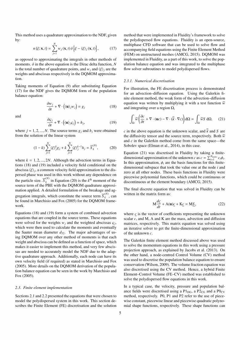
The polydispersed BFS simulation was run for three differ-ent fixed meshes, for Case 1, to study mesh convergence inthis problem. Details of the three fixed meshes, referred to asCoarse, Medium and Fine mesh, can be found in Table 9. Avery fine mesh simulation, called the Superfine mesh, was alsorun with a total of 147,308 nodes and a characteristic mesh sizeof 0.2 mm. This Superfine mesh was selected as a proxy forthe exact solution to the problem, for the purpose of calculatingerrors in the solutions produced by the other three meshes. Allfixed meshes were generated using the open-source mesh gen-eration software Gmsh (Geuzaine and Remacle, 2009). Figure10 shows a part of the Coarse mesh that was used in the simu-lation. The unstructured nature of the mesh can be seen clearlyalong with the refined elements near the step. The mesh ele-ments near the step were four times smaller than usual to cap-ture the strong field variations in that region. All other fixedmeshes, except for their finer element size, were similar to the

12

Table 8Boundary Conditions (BCs) for the population balance equation solution fields used in the polydispersed backward facing step simulation. BCs are presented forthe weights (w1 and w2) and the weighted abscissas (ς1 and ς2). n here refers to the normal coordinate

Boundary w1 w2 ς1 ς2

Inlet 1.125 × 1012 9.514 × 1011 3.020 × 107 5.351 × 107

Walls no flux no flux no flux no flux

Outlet∂w1

∂n= 0

∂w2

∂n= 0

∂ς1

∂n= 0

∂ς2

∂n= 0

Water Sauter mean diameter (µm)

50 60 70 80

Figure 8: Sauter mean diameter of water drops for the aggregation dominated case (Case 1) at four different times: (top to bottom) 0.25 s, 0.5 s, 0.75 s and 1.0 s.The primary and the secondary recirculation zones for the SMD can be seen.

Water Sauter mean diameter (µm)

32 36 40 44 48 50

Figure 9: Sauter mean diameter of water drops for the breakage dominated case (Case 2) at four different times: (top to bottom) 0.25 s, 0.5 s, 0.75 s and 1.0 s. Theprimary and the secondary recirculation zones for the SMD can be seen.

Table 9Details of the three fixed meshes used for the mesh convergence analysis ofthe solution of polydispersed backward facing step in Fluidity.

Mesh Mesh nodes Mesh size (mm)Coarse 19,825 0.55Medium 24,100 0.5Fine 65,967 0.3

Coarse mesh.

Jacobs et al. (2013) showed a second order convergence forboth velocity and pressure in multiphase flow simulations forthe P1DG-P2 element pair in Fluidity. The same velocity-pressure element pair was used here, with an additional pop-ulation balance equation that was discretised using the controlvolume scheme. To study the mesh convergence of the popula-tion balance equation, the fixed mesh simulations were run upto 1 s and the error in the Sauter mean diameter of water dropswas plotted as a function of mesh size, as illustrated in Figure11. The order of convergence obtained was close to the ex-

13

Figure 10: Fixed mesh used in the simulation of the polydispersedwater-in-oil emulsion. This is the Coarse mesh with a characteristic mesh sizeof 0.55 mm. All other fixed meshes were similar to this Coarse mesh exceptfor a different mesh size.

10−4 10−3

Characteristic mesh size (m)

10−8

10−7

Err

orin

SMD

(L2-n

orm

)

Fixed meshFirst order convergence

Figure 11: Convergence plot for the Sauter mean diameter of water drops.The population balance equation converged to first order as expected.

pected first-order convergence for the control volume discreti-sation method.

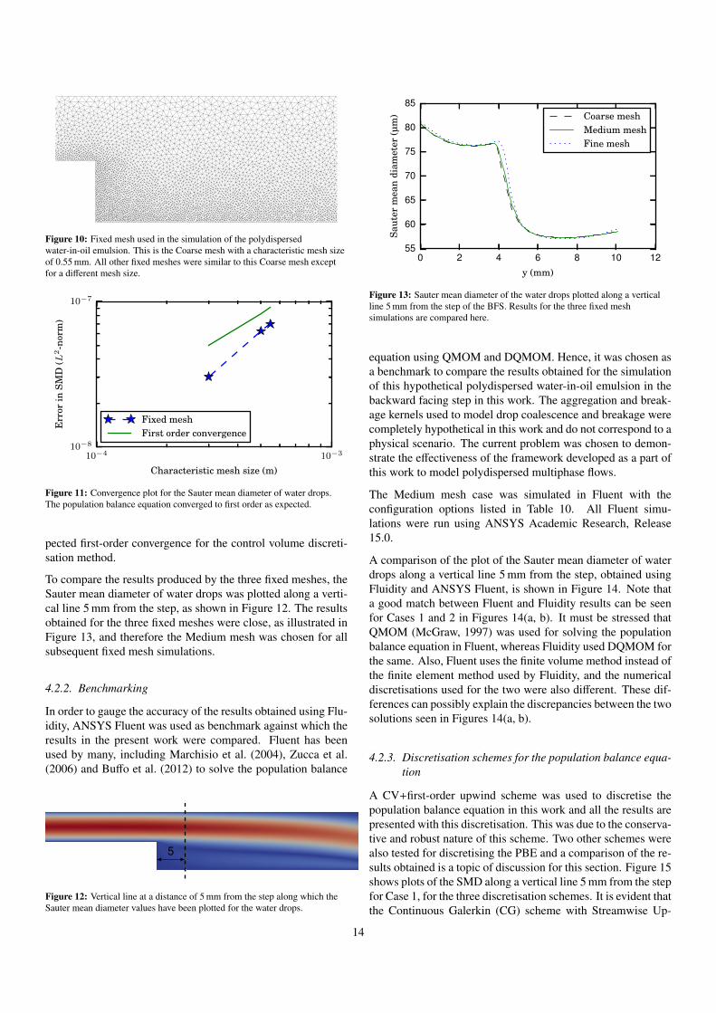
To compare the results produced by the three fixed meshes, theSauter mean diameter of water drops was plotted along a verti-cal line 5 mm from the step, as shown in Figure 12. The resultsobtained for the three fixed meshes were close, as illustrated inFigure 13, and therefore the Medium mesh was chosen for allsubsequent fixed mesh simulations.

4.2.2. Benchmarking

In order to gauge the accuracy of the results obtained using Flu-idity, ANSYS Fluent was used as benchmark against which theresults in the present work were compared. Fluent has beenused by many, including Marchisio et al. (2004), Zucca et al.(2006) and Buffo et al. (2012) to solve the population balance

5

Figure 12: Vertical line at a distance of 5 mm from the step along which theSauter mean diameter values have been plotted for the water drops.

0 2 4 6 8 10 12

y (mm)

55

60

65

70

75

80

85

Saut

erm

ean

diam

eter

(µm

) Coarse meshMedium meshFine mesh

Figure 13: Sauter mean diameter of the water drops plotted along a verticalline 5 mm from the step of the BFS. Results for the three fixed meshsimulations are compared here.

equation using QMOM and DQMOM. Hence, it was chosen asa benchmark to compare the results obtained for the simulationof this hypothetical polydispersed water-in-oil emulsion in thebackward facing step in this work. The aggregation and break-age kernels used to model drop coalescence and breakage werecompletely hypothetical in this work and do not correspond to aphysical scenario. The current problem was chosen to demon-strate the effectiveness of the framework developed as a part ofthis work to model polydispersed multiphase flows.

The Medium mesh case was simulated in Fluent with theconfiguration options listed in Table 10. All Fluent simu-lations were run using ANSYS Academic Research, Release15.0.

A comparison of the plot of the Sauter mean diameter of waterdrops along a vertical line 5 mm from the step, obtained usingFluidity and ANSYS Fluent, is shown in Figure 14. Note thata good match between Fluent and Fluidity results can be seenfor Cases 1 and 2 in Figures 14(a, b). It must be stressed thatQMOM (McGraw, 1997) was used for solving the populationbalance equation in Fluent, whereas Fluidity used DQMOM forthe same. Also, Fluent uses the finite volume method instead ofthe finite element method used by Fluidity, and the numericaldiscretisations used for the two were also different. These dif-ferences can possibly explain the discrepancies between the twosolutions seen in Figures 14(a, b).

4.2.3. Discretisation schemes for the population balance equa-tion

A CV+first-order upwind scheme was used to discretise thepopulation balance equation in this work and all the results arepresented with this discretisation. This was due to the conserva-tive and robust nature of this scheme. Two other schemes werealso tested for discretising the PBE and a comparison of the re-sults obtained is a topic of discussion for this section. Figure 15shows plots of the SMD along a vertical line 5 mm from the stepfor Case 1, for the three discretisation schemes. It is evident thatthe Continuous Galerkin (CG) scheme with Streamwise Up-

14

Table 10Simulation configuration settings for Fluent used for modelling the polydispersed water-in-oil emulsion in a backward facing step.

Solver pressure-basedtransient

Model multiphase 2 Eulerian phasesimplicitSchiller–Naumann dragdrop diameter: Sauter mean diame-ter

viscous laminarpopulation balance QMOM

4 momentsUDFs for breakage and aggregationkernels

Boundary conditions walls stationary wallsinlet velocity: UDF for parabolic veloc-

itywater volume fraction = 0.1water moments specified

outlet pressure outletSolution methods P-V coupling coupled scheme

spatial discretisation gradients: least squares cell basedmomentum: third-order MUSCLvolume fraction: first-order upwindmoments: first-order upwind

transient discretisation first-urder implicitRelaxation parameters momentum 0.75

pressure 0.75volume fraction 0.5moments 0.5

15

0 2 4 6 8 10 12

y (mm)

55

60

65

70

75

80

85

Saut

erm

ean

diam

eter

(µm

) FluidityFluent

(a) Case 1

0 2 4 6 8 10 12

y (mm)

32

34

36

38

40

42

44

Saut

erm

ean

diam

eter

(µm

) FluidityFluent

(b) Case 2

Figure 14: Fluidity results benchmarked against ANSYS Fluent results for:(a) the aggregation dominated case (Case 1), and (b) the breakage dominatedcase (Case 2). Sauter mean diameter of the water drops has been plotted alongthe vertical line shown in Figure 12, for the two solvers.

0 2 4 6 8 10 12

y (mm)

55

60

65

70

75

80

85

Saut

erm

ean

diam

eter

(µm

) CV UpwindCV FE SwebyCG SUPG

Figure 15: Comparison of different discretisation schemes tried for thepopulation balance equation. Plot of the Sauter mean diameter along a verticalline 5 mm from the step has been shown for the aggregation dominant case(Case 1) at t =1 s. Continuous Galerkin (CG) discretisation method with aStreamwise Upwind Petrov Galerkin (SUPG) stabilisation showed the mostaccurate result with minimum diffusivity amongst all discretisation schemesthat were tested. Despite this, the CV scheme, with first-order upwinddiscretisation for the convective terms, was chosen for all polydispersed flowsimulations due to its conservative and stable nature, unlike other schemes.

wind Petrov Galerkin (SUPG) stabilisation for the convectiveterms was the least diffusive of all, as seen from the slope ofthe line between y=4 mm and y=6 mm, and hence was able toresolve the primary recirculation boundary most accurately. Itwas also able to resolve the top boundary layer, as displayed bythe SMD value around y=10 mm. On the other hand, the Con-trol Volume (CV) scheme with first-order upwind discretisationfor the convection terms was most diffusive. Somewhere in themiddle was the CV scheme with a finite element discretisationfor convective terms, with a Sweby limiter (Sweby, 1984), asshown in Figure 15.

Figure 16 shows the surface plots for the water SMD at t=1 sfor the three schemes. Accuracy of the CG and the CV+FEschemes is visually apparent, through the better resolution ofthe two recirculation zones, over the CV+first-order upwindscheme. Despite the advantages of the two accurate schemes,the CV+first-order upwind scheme was chosen for all simula-tions due to its conservative and monotonic nature, which en-sured that the moments were conserved and the method wasunconditionally stable.

Results for the polydispersed multiphase flow simulations werepresented in this section and the effectiveness of the finiteelement framework of Fluidity in modelling such flows wasdemonstrated. Offering an alternative over the other (very few)available commercial and non-commercial flow solvers that areable to deal with multiphase polydispersed flows, Fluidity’sFE–CV hybrid approach was shown to be able to gather thebest of both worlds—finite element and control volume—andsimulate such flows with good accuracy.

The framework of Fluidity is parallelised and all fixed mesheswere decomposed and distributed among different processorsto be able to solve the simulations quickly. All simulations pre-sented here were parallelised to 8 cores. To make the simu-

16

Water Sauter mean diameter (µm)

50 60 70 80

Figure 16: Sauter mean diameter of water drops for Case 1 at t =1 s for three different discretisation schemes for the population balance equation. From top tobottom: CV+first-order upwind, CV+finite element (Sweby limiter) and CG+SUPG stabilisation. CG+SUPG discretisation was able to resolve the tworecirculation zones better than the two other schemes. Despite this, the control volume scheme, with first-order upwind discretisation for the convective terms, waschosen for all polydispersed flow simulations due to its conservative and stable nature, unlike other schemes.

lation process more efficient, mesh adaptivity, as discussed inSection 2.4, was also introduced in the simulations and the re-sults demonstrating the excellent improvement obtained usingthis process are discussed in the next section.

4.3. Mesh adaptivity

The transient flow field results shown in the previous section(Section 4.2) were all for a fixed mesh, which did not changewith time. Such a fixed mesh can rarely be optimum for adynamic problem like the one under consideration. Optimummesh node positioning cannot be decided in advance as the flowfeatures are changing continuously due to the inherent complexdynamics of the problem. Mesh adaptivity offers a way to han-dle this issue by adapting the mesh in time and hence, was ap-plied to the polydispersed water-in-oil emulsion flow problemin this work. This section presents and analyses the results foran adaptive mesh simulation of the polydispersed flow and com-pares the solution errors and runtimes to the fixed mesh simu-lations presented in the previous section.

An adaptive mesh simulation was set up for the aggregationdominated (Case 1) water-in-oil emulsion problem in a BFS,where the mesh was adapted to the water droplet size and ve-locity. The reason for this choice was that water droplet sizeand velocity were the fields of interest in this work and the otherfields were observed to vary similar to these two in space. Atfirst, the mesh was adapted to the water Sauter mean diameteronly, as this was the most important scalar field in this polydis-persed flow problem. However, it was realised that the meshadapted to the water SMD alone was not able to resolve thestrong variations in water velocity in the y-direction when themesh became excessively coarse in regions away from the re-circulation zone boundaries. The increased error in flow veloc-ity associated with the coarse mesh in these regions requiredthe inclusion of the water velocity in the list of fields the meshwas adapted to. Also, a bound was set on the maximum mesh

resolution to prevent it from going excessively coarse in “non-critical” regions.

The interpolation error bound values used for the calculationof the error metric (see Section 2.4) are shown in Table 11. Acouple of quick mesh adaptivity trials were conducted with dif-ferent combinations of the interpolation errror bound values tocome up a good set of values as given in Table 11. Absoluteinterpolation error values were used here instead of the relativeones to ensure consistency in the specification of mesh resolu-tion over space.

Table 11Interpolation error bound for the fields that the mesh was adapted to.

Field Interpolation error bound(absolute)

Sauter mean diameter (d32) 2.5 × 10−7 mWater velocity (ud) (0.01, 0.005) m s−1

A number of other numerical parameters associated with themesh adaptivity settings were adjusted and their values areshown in Table 12. Adaptivity subroutine was called after ev-ery 100 time steps, i.e. every 0.001 s in the simulation. Thisensured that the mesh was adapted just enough so as to notchange drastically between any two adapts, and the computa-tional effort spent in adaptivity was also kept to a minimum.Therefore, a total of 1000 mesh adaptivity cycles were carriedout in an overall simulation time of 1 s. Bounds were speci-fied for the minimum and maximum mesh edge lengths to pre-vent the mesh from becoming excessively fine or coarse. Theconsistent interpolation method was used to interpolate the var-ious scalar, vector and tensor fields from the pre-adapt meshto the post-adapt mesh. More details on the implementation ofmesh adaptivity in Fluidity can be found in the Fluidity Manual(AMCG, 2015).

Since the simulation was performed in a parallelised framework

17

on a multi-core machine, 15 adapt iterations had to be per-formed during each adaptivity cycle instead of just one. Nodesshared between different processors remain locked while the in-dividual processors optimise their meshes, and load balancing isonly performed after an adaptive iteration is completed. Hence,15 adapt iterations were necessary to ensure that all nodes wereconsidered for the adaptivity process at least once (Devine et al.,2002; AMCG, 2015).

Table 12Adaptivity settings used for the adaptive mesh simulation of the polydispersedwater-in-oil emulsion in Fluidity.

Number of time steps between two adapts 100Gradation parameter 1.3Minimum edge length (m) 10−4

Maximum edge length (m) 0.01Number of adaptive iterations for parallel adaptivity 15Field interpolation method consistent

All flow and population balance discretisations were exactlythe same as for the fixed mesh case in Section 4.2. Theunconditionally-stable first-order upwind scheme was used todiscretise the convective fluxes in the advection equations forvolume fraction and population balance equation scalars. Otherconditionally-stable schemes (such as finite element, trape-zoidal, etc.) are stable for only a range of values of the gridPeclet number (Donea and Huerta, 2003), even when used inconjunction with slope limiters. Mesh adaptivity can lead to thegeneration of coarse elements which can then result in high val-ues for the Peclet number in those regions making such schemessensitive to the adapting mesh. The use of the unconditionally-stable first-order upwind scheme in this work avoids this prob-lem.

Initial mesh for the adaptive simulation was generated usingthe open-source mesh generation software Gmsh (Geuzaine andRemacle, 2009). Simulation results for the adaptive mesh sim-ulation described above are shown in Figure 17. Water Sautermean diameter and the corresponding adapted mesh are pre-sented for three different simulation times. Although the meshwas also adapted to the two components of water velocity, watervelocity contours have not been shown here. The mesh in Fig-ure 17 clearly displays its non-homogeneous, anisotropic char-acter, as expected, and conforms with the variations in the SMDover space. Elongated elements resolved the recirculation zoneboundaries by concentrating node density in only the normal di-rection, by using the anisotropic property of the adapted mesh.Mesh anisotropy in the y-direction in the interior of the BFScomes from the inclusion of the flow velocity to the mesh adap-tivity parameters.

A plot of the Sauter mean diameter along a vertical line 5 mmfrom the step is presented in Figure 18 for comparing the adap-tive mesh simulation to two fixed meshes—Coarse mesh andFine mesh. The Adaptive mesh was able to resolve the pri-mary recirculation zone more accurately than the other two

fixed meshes by increasing the mesh resolution near the recir-culation zone boundary, and this can be seen from the steeperslope of the Sauter mean diameter plot between y=4 mm andy=6 mm. Figure 18 also shows that the Adaptive mesh wasable to resolve the top boundary layer better than the other twomeshes. All this was made possible by optimising the place-ment of mesh nodes in the appropriate regions.

Figures 19 and 20 show the number of mesh nodes and run-times, respectively for the Adaptive mesh simulation. The num-ber of nodes for the Adaptive mesh simulation, as shown in Fig-ure 19, always stayed below the number of Coarse mesh nodeswith the maximum number of Adaptive mesh nodes still 30 per-cent lower than the fixed Coarse mesh. This number was muchlower when compared to the Fine mesh. Similar behaviour wasalso displayed in the comparison of the simulation runtimes forthe three meshes, as seen in Figure 20. The Adaptive mesh sim-ulation took 30 percent less time to run than what the Coarsemesh took. Since this runtime for the Adaptive mesh simula-tion included both the solution computation time and the timeneeded for mesh adaptivity, it is clear that the cost of adaptiv-ity was negligible compared to the solution computation timefor this problem. The cost associated with an expensive inter-polation method, such as the Galerkin projection interpolation,in the presence of large number of flow fields could potentiallydecrease the overall improvement in the efficiency obtained us-ing mesh adaptivity, but it clearly was not the case in this workthat used the consistent interpolation method.

It was shown in the previous paragraphs that the adaptive meshsimulation in this work was able to produce non-homogeneous,anisotropic, unstructured meshes, which conformed well withthe variations in the water droplet size distribution. Moreover,the selected adaptive mesh simulation was quicker than boththe fixed Coarse and Fine meshes, with the time taken for meshadaptivity being small. Still, it needs to be shown quantitativelythat the overall solution produced by the Adaptive mesh simu-lation was more accurate than the fixed mesh, if this techniqueis to serve any importance in the modelling of polydispersedmultiphase flows. Figure 21 presents the L2-norm of the errorin the Sauter mean diameter (of water drops) with time, for thethree meshes. The errors for the Adaptive mesh simulation werelower than those for the Coarse mesh beyond t=0.4 s. All errorshere were calculated with respect to the Superfine fixed meshsolution, as discussed in Section 4.2. The Adaptive mesh solu-tion error was 40 percent smaller than the Coarse mesh error att=1 s.

It can be summarised that mesh adaptivity produced quickerand more accurate solution than the corresponding fixed meshsimulation in this work. It is safe to generalise here that poly-dispersed multiphase flows can be simulated more efficientlyusing this technique when appropriate mesh adaptivity param-eters are chosen in the simulation. The cost of mesh adaptivityin these simulations is negligible when compared to the solu-tion computation time and hence should be preferred over otherfixed solvers when simulating polydispersed multiphase flowsin two or three spatial dimensions.

18

(a) t=0.50 s

(b) t=0.75 s

(c) t=1.0 s

Water Sauter mean diameter (µm)

50 58 66 74 82

Figure 17: Water Sauter mean diameter and the corresponding mesh for the adaptive mesh simulation of the polydispersed water-in-oil emulsion. (a) t=0.50 s, (b)t=0.75 s and (c) t=1.0 s.

19

0 2 4 6 8 10 12

y (mm)

55

60

65

70

75

80

85

Saut

erm

ean

diam

eter

(µm

) Coarse meshFine meshAdaptive mesh

Figure 18: Sauter mean diameter of the water drops plotted along a verticalline 5 mm from the step of the BFS. Result for the Adaptive mesh is comparedwith the Coarse mesh and the Fixed mesh results.

0.0 0.2 0.4 0.6 0.8 1.0

time (s)

0

15000

30000

45000

60000

75000

Num

ber

ofm

esh

node

s 65967 nodes

19825 nodes

Fine meshCoarse meshAdaptive mesh

Figure 19: Plot of the number of mesh nodes with time for the Adaptive mesh,Coarse mesh and the Fine mesh.

Coarse Adapt Fine0

50

100

150

200

250

300

350Runtime (hrs)

Figure 20: Runtimes (walltime) compared for the Coarse mesh, Adaptivemesh and Fine mesh simulations. All runtimes are presented for 8-coreparallel runs. Mesh was adapted after every 0.001 s, i.e. a total of 1000 meshadaptivity cycles in the 1 s simulation.

5. Conclusions

An efficient, open-source finite element framework to solvepolydispersed flow problems was presented in this paper. CFDbased modelling of polydispersed flows in the open-source Flu-

0.0 0.2 0.4 0.6 0.8 1.0

time (s)

0.0

0.5

1.0

1.5

2.0

2.5

Perc

ent

erro

r(L

2-n

orm

)

Fine meshCoarse meshAdaptive mesh

Figure 21: Error in the Adaptive mesh simulation compared with Coarse andFine mesh results. L2-norm of the percentage error in the Sauter meandiameter has been plotted here with time.

idity code was implemented using a coupled Eulerian–Eulerianpopulation balance modelling approach. Marchisio and Fox(2005)’s direct quadrature method of moments was utilisedfor solving the population balance equation and the imple-mentation was verified successfully using McCoy and Madras(2003)’s analytical solution.

The present implementation is general for up to three spatial di-mensions, but for simplicity the code was benchmarked againsta commercial CFD software for a hypothetical two-dimensionalwater-in-oil emulsion problem in a backward facing step do-main. A hybrid finite element–control volume method for solv-ing the coupled system of equations gave the best result. In thismethod the velocity-pressure equation set was discretised usingthe P1DG-P2 element pair and the volume fraction equation andthe population balance equation were discretised using the con-trol volume approach. A good match between the results pro-duced by the present implementation and the commercial CFDsoftware ANSYS Fluent, was obtained. Although a few otherdiscretisations were tested for the population balance equation,the hybrid FE–CV method was the most robust of all as the CVmethod was conservative and stable.

The hypothetical backward facing step problem in this workwas explicitly assumed to be laminar to demonstrate the cou-pling between the Eulerian–Eulerian flow equations with thepopulation balance equation without bringing in the complex-ities of modelling turbulence. Real applications, though, areseldom laminar and turbulence equations need to be coupled tothe above set of equations, which will be discussed in futurework by the authors.

Adaptive mesh refinement was also applied to the polydispersedBFS simulation. The finite element mesh in this case wasadapted in time to the water Sauter mean diameter and velocityfields so that these fields satisfied a specific resolution require-ment on the resulting adapted mesh. Fully-unstructured, non-homogeneous, anisotropic meshes were generated by the meshadaptivity subroutine. The adapted meshes conformed remark-ably with the flow fields that they were adapted to. An excel-lent improvement in the solver efficiency was reported by the

20

use of mesh adaptivity in this problem. The errors produced bythe adaptive mesh simulation were 40 percent smaller than thecorresponding errors in the fixed mesh simulation. The adap-tive mesh simulation, after taking into account the time takento adapt meshes, was 35 percent faster than the correspondingfixed mesh simulation.

Based on the results obtained in this work, it can be concludedthat the open-source finite element framework of Fluidity is ac-curate and provides an efficient alternative to the other availablefinite volume/ control volume CFD packages for solving poly-dispersed flow problems. The present implementation allowsfor a single continuous phase with many dispersed phases, witheach dispersed phase containing as many population balanceequations as required. Experimental validation and the use ofmore than one population balance equation per phase to modela three-phase three-dimensional industrial polydispersed flowproblem will be presented in the future work by the authors. Al-though the current implementation can handle only one internalvariable in the NDF, the ability to calculate multidimensionalmoments of the NDF will be added in the future to model morecomplex dispersed phases. With the use of mesh adaptivity in ahighly-parallelised distributed computational environment, theopen-source finite element framework presented in this paper(employing the population balance modelling approach) canprove to be an efficient tool for modelling industrial-scale mul-tiphase polydispersed flow problems.

Acknowledgements

We would like to thank the members of the Applied Modellingand Computation Group with whom we had interesting dis-cussions regarding the work presented in this paper. We alsoacknowledge the support received from the High PerformanceComputing Service at Imperial College London. Special thanksto Sam Parkinson for the initial work on the implementationof DQMOM in Fluidity. GB would like to thank AjayendarReddy and Deepak Sachan for proofreading a first draft of thismanuscript and providing their valuable suggestions.

Appendix A. Length-based formulation of the analyticalsolution

The length-based version of the problem developed by McCoyand Madras (2003) can be written as follows:

For an initial number density function given by

nξ(ξ, 0

)= 3ξ2 m0(0)2

m3exp

(−ξ3 m0(0)

m3

), (A.1)

and breakage and aggregation kernels given by

ν = 2, (A.2)

a(ξ)

= s ξ3, (A.3)

b(ξ|ξ1

)=

3ξ2

ξ13 if ξ < ξ1,

0 otherwise(A.4)

andβ = constant, (A.5)

there exists an analytical solution to the population balanceequation (Equation (9)) when u = 0, which is given as:

nξ(ξ, t

)= k1ξ

2exp(−k2ξ

3). (A.6)

k1 and k2 here are given by:

k1 = 3 n2ξ(t)

m0(0)2

m3(A.7)

andk2 = nξ(t)

m0(0)m3

, (A.8)

where

nξ(t) = nξ(∞)

1 + nξ(∞) tanh(nξ(∞) m0(0)βt

2

)nξ(∞) + tanh

(nξ(∞) m0(0)βt

2

) . (A.9)

The constant nξ(∞) is given in terms of the breakage and aggre-gation kernels as:

nξ(∞) =

(2 s m3

β

)1/2 (1

m0(0)

). (A.10)

m0(0) and m3 in all the above equations are specified as initialconditions.

Since DQMOM was used in this work, the moments of theNDF given in Equation (A.6) were needed for the calculationof the Sauter mean diameter, d32, for verification. The first fourlength-based moments of this function can be written as:

m0(t) = m0(0) nξ(t), (A.11)

m1(t) =k1

3k24/3 Γ

(43

), (A.12)

m2(t) =k1

3k25/3 Γ

(53

), (A.13)

andm3(t) = m3, (A.14)

where Γ is the standard gamma function. These equations werealso used for the calculation of the initial moment set for ini-tialising the polydispersed flow problem.

References

Abbasi E, Arastoopour H. Numerical analysis and implementation of finite do-main complete trial functions method of moments (FCMOM) in CFD codes.Chem Eng Sci 2013;102:432–441.

AMCG. Fluidity manual v4.1.12. Imperial College London 201504;http://dx.doi.org/10.6084/m9.figshare.1387713.

21

Nomenclature

AbbreviationsBFS Backward Facing StepCG Continuous GalerkinCV Control VolumeDG Discontinuous GalerkinDQMOM Direct Quadrature Method of MomentsFE Finite ElementFEM Finite Element MethodNDF Number Density FunctionPBE Population Balance EquationQMOM Quadrature Method of MomentsSMD Sauter Mean DiameterSUPG Streamwise Upwind Petrov GalerkinUppercase Roman SymbolsBB Birth term due to breakageBC Birth term due to coalescenceCD Drag coefficient used in the interphase drag force termDB Death term due to breakageDC Death term due to coalescenceH Hessian tensor of the solution field (in mesh adaptivity)M Riemannian mesh metric used in mesh adaptivityN Number of weights or abscissas used in the approxi-

mation of the number density function in the DQMOMmethod

Nphases Number of phases in the multiphase problemRec Continuous phase Reynolds numberRed Dispersed phase Reynolds numberS ξ Source term in the population balance equationLowercase Roman Symbolss Constant coefficient in the power law breakage frequencya Breakage frequencyb Breakage daughter distribution functiond Dispersed phase diameterd32 Sauter mean diameter

g j jth source term in the DQMOM weight equationh j jth source term in the DQMOM weighted abscissa equa-

tionmk kth moment of the number density functionn Number density function used in the PBEp Common pressure field for all phasest Time coordinateu x-component of velocityw j jth weight in the DQMOM approximation of the NDFf D Interphase drag forcefi Interphase force acting on phase i due to all other phasesg Acceleration due to gravityui Velocity of phase ix Vector of external coordinates in the NDF, or spatial co-

ordinatesv y-component of velocityGreek Symbolsα Volume fractionβ Aggregation frequencyε User-specified interpolation error bound for mesh adap-

tivityµ Dynamic viscosityν Average number of dispersed particles formed after

breakageρ Densityς Weighted abscissa in the DQMOM equation (ς j =

w j〈ξ〉 j)ξ Internal coordinate in the NDF〈ξ〉 j jth abscissa in the DQMOM approximation of the NDF

τi Deviatoric stress tensor for phase iSubscriptsc, d Continuous and dispersed phases, respectivelyi Phase

22

Armaly BF, Durst F, Pereira J, Schonung B. Experimental and theoretical in-vestigation of backward-facing step flow. J Fluid Mech 1983;127:473–496.

Babuska I, Rheinboldt WC. Error estimates for adaptive finite element compu-tations. SIAM J Numer Anal 1978;15(4):736–754.

Bannari R, Kerdouss F, Selma B, Bannari A, Proulx P. Three-dimensional math-ematical modeling of dispersed two-phase flow using class method of pop-ulation balance in bubble columns. Comput Chem Eng 2008;32(12):3224–3237.

Bassi F, Rebay S. A high-order accurate discontinuous finite element methodfor the numerical solution of the compressible Navier–Stokes equations. JComput Phys 1997;131(2):267–279.

Becker PJ, Puel F, Dubbelboer A, Janssen J, Sheibat-Othman N. Coupled pop-ulation balance–CFD simulation of droplet breakup in a high pressure ho-mogenizer. Comput Chem Eng 2014;68:140–150.

Bowen RM. Theory of mixtures. In: Eringen AC, editor. Continuum physics,vol. III Waltham: Academic Press; 1976.

Brennen CE. Fundamentals of multiphase flow. Cambridge University Press;2005.

Buffo A, Vanni M, Marchisio DL. Multidimensional population balance modelfor the simulation of turbulent gas–liquid systems in stirred tank reactors.Chem Eng Sci 2012;70:31–44.

Buwa VV, Ranade VV. Dynamics of gas–liquid flow in a rectangular bubblecolumn: experiments and single/multi-group CFD simulations. Chem EngSci 2002;57(22):4715–4736.

Chan T, Liu Y, Chan C. Direct quadrature method of moments for the exhaustparticle formation and evolution in the wake of the studied ground vehicle.J Aerosol Sci 2010;41(6):553–568.

Chen P, Sanyal J, Dudukovic M. CFD modeling of bubble columns flows:implementation of population balance. Chem Eng Sci 2004;59(22):5201–5207.

Clift R, Grace JR, Weber ME. Bubbles, drops, and particles. Academic Press;1978.

Cotter CJ, Ham DA, Pain CC. A mixed discontinuous/continuous finite elementpair for shallow-water ocean modelling. Ocean Modell 2009;26(1):86–90.

Devine K, Boman E, Heaphy R, Hendrickson B, Vaughan C. Zoltan datamanagement services for parallel dynamic applications. Comput Sci Eng2002;4(2):90–96.

Donea J, Huerta A. Finite element methods for flow problems. John Wiley &Sons; 2003.

Elman HC, Silvester DJ, Wathen AJ. Finite elements and fast iterative solvers:with applications in incompressible fluid dynamics. Oxford UniversityPress; 2014.

Farrell P, Piggott M, Pain C, Gorman G, Wilson C. Conservative interpolationbetween unstructured meshes via supermesh construction. Comput MethAppl Mech Eng 2009;198(33):2632–2642.

Favero JL, Silva LFLR, Lage PLC. Modeling and simulation of mixing inwater-in-oil emulsion flow through a valve-like element using a populationbalance model. Comput Chem Eng 2015;75:155–170.

Frenklach M, Harris SJ. Aerosol dynamics modeling using the method of mo-ments. J Colloid Interface Sci 1987;118(1):252–261.

Geuzaine C, Remacle JF. Gmsh: A 3-D finite element mesh generatorwith built-in pre-and post-processing facilities. Int J Numer Meth Eng2009;79(11):1309–1331.

Gordon RG. Error bounds in equilibrium statistical mechanics. J Math Phys1968;9:655.

Gresho PM, Chan ST. Solving the incompressible Navier–Stokes equationsusing consistent mass and a pressure Poisson equation. Lawrence LivermoreNational Lab., CA (USA); 1988.

Ishii M, Zuber N. Drag coefficient and relative velocity in bubbly, droplet orparticulate flows. AlChE J 1979;25(5):843–855.

Jacobs CT, Collins GS, Piggott MD, Kramer SC, Wilson CRG. Multiphaseflow modelling of volcanic ash particle settling in water using adaptive un-structured meshes. Geophys J Int 2013;192(2):647–665.

Marchal P, David R, Klein J, Villermaux J. Crystallization and precipitationengineering—I. An efficient method for solving population balance in crys-tallization with agglomeration. Chem Eng Sci 1988;43(1):59–67.

Marchisio DL, Fox RO. Computational models for polydisperse particulate andmultiphase systems. Cambridge University Press; 2013.

Marchisio DL, Fox RO. Solution of population balance equations using thedirect quadrature method of moments. J Aerosol Sci 2005;36(1):43–73.

Marchisio DL, Pikturna JT, Fox RO, Vigil RD, Barresi AA. Quadrature method

of moments for population-balance equations. AlChE J 2004;49(5):1266–1276.

McClure DD, Norris H, Kavanagh JM, Fletcher DF, Barton GW. Validation of acomputationally efficient computational fluid dynamics (CFD) model for in-dustrial bubble column bioreactors. Ind Eng Chem Res 2014;53(37):14526–14543.

McCoy B, Madras G. Analytical solution for a population balance equationwith aggregation and fragmentation. Chem Eng Sci 2003;58(13):3049–3051.

McGraw R. Description of aerosol dynamics by the quadrature method of mo-ments. Aerosol Sci Technol 1997;27(2):255–265.

Pain C, Umpleby A, De Oliveira C, Goddard A. Tetrahedral mesh optimisa-tion and adaptivity for steady-state and transient finite element calculations.Comput Meth Appl Mech Eng 2001;190(29):3771–3796.

Piggott M, Farrell P, Wilson C, Gorman G, Pain C. Anisotropic mesh adap-tivity for multi-scale ocean modelling. Philos Trans R Soc London, Ser A2009;367(1907):4591–4611.

Prakash AV, Chaudhury A, Barrasso D, Ramachandran R. Simulation of popu-lation balance model-based particulate processes via parallel and distributedcomputing. Chem Eng Res Des 2013;91(7):1259–1271.

Prosperetti A, Tryggvason G. Computational methods for multiphase flow.Cambridge university press; 2007.

Ramkrishna D. Population balances: Theory and applications to particulatesystems in engineering. Academic press; 2000.

Roudsari SF, Turcotte G, Dhib R, Ein-Mozaffari F. CFD modeling of the mixingof water in oil emulsions. Comput Chem Eng 2012;45:124–136.

Santos FP, Senocak I, Favero JL, Lage PLC. Solution of the population balanceequation using parallel adaptive cubature on GPUs. Comput Chem Eng2013;55:61–70.

Sanyal J, Marchisio DL, Fox RO, Dhanasekharan K. On the comparison be-tween population balance models for CFD simulation of bubble columns.Ind Eng Chem Res 2005;44(14):5063–5072.

Schiller L, Naumann Z. A drag coefficient correlation. Vdi Zeitung1935;77(318):51.

Selma B, Bannari R, Proulx P. Simulation of bubbly flows: Comparison be-tween direct quadrature method of moments (DQMOM) and method ofclasses (CM). Chem Eng Sci 2010;65(6):1925–1941.

Silva L, Damian R, Lage P. Implementation and analysis of numerical solutionof the population balance equation in CFD packages. Comput Chem Eng2008;32(12):2933–2945.

Silva L, Lage P. Development and implementation of a polydispersed multi-phase flow model in OpenFOAM. Comput Chem Eng 2011;35(12):2653–2666.

Sweby PK. High resolution schemes using flux limiters for hyperbolic conser-vation laws. SIAM J Numer Anal 1984;21(5):995–1011.

Szilagyi B, Agachi Pc, Barabas R, Lakatos BG. Coupled Population Balance-CFD Modelling of a Continuous Precipitation Reactor. In: Klemes JJ, Var-banov PP, Liew PY, editors. 24th European Symposium on Computer AidedProcess Engineering, vol. 33 of Computer Aided Chemical Engineering;2014.p. 187–192.

Tabib MV, Roy SA, Joshi JB. CFD simulation of bubble column—an analysisof interphase forces and turbulence models. Chem Eng J 2008;139(3):589–614.

Vasilevskii YV, Lipnikov K. An adaptive algorithm for quasioptimal mesh gen-eration. Comput Math Math Phys 1999;39(9):1468–1486.

Wilson C. Modelling multiple-material flows on adaptive unstructured meshes.PhD thesis, Imperial College London; 2009.

Yeoh G, Cheung S, Tu J. On the prediction of bubble size distribution andvoid fraction in vertical gas-liquid flows. J Comput Multiphase Flows2012;4(1):1–22.

Yeoh GH, Cheung CP, Tu J. Multiphase flow analysis using population balancemodeling: bubbles, drops and particles. Butterworth-Heinemann; 2013.

Zucca A, Marchisio DL, Barresi AA, Fox RO. Implementation of the popula-tion balance equation in CFD codes for modelling soot formation in turbu-lent flames. Chem Eng Sci 2006;61(1):87–95.

23