Algorithmica (1994) 12:436-457 Algorithmica �9 1994 Springer-Verlag New York Inc.

Polynomial Algorithms for Linear Programming over the Algebraic Numbers 1

I. Adler 2 and P. A. Beling 3

Abstract. We derive a bound on the computational complexity of linear programs whose coefficients are real algebraic numbers. Key to this result is a notion of problem size that is analogous in function to the binary size of a rational-number problem. We also view the coefficients of a linear program as members of a finite algebraic extension of the rational numbers. The degree of this extension is an upper bound on the degree of any algebraic number that can occur during the course of the algorithm, and in this sense can be viewed as a supplementary measure of problem dimension. Working under an arithmetic model of computation, and making use of a tool for obtaining upper and lower bounds on polynomial functions of algebraic numbers, we derive an algorithm based on the ellipsoid method that runs in time bounded by a polynomial in the dimension, degree, and size of the linear program. Similar results hold under a rational number model of computation, given a suitable binary encoding of the problem input.

Key Words. Linear programming, Algebraic numbers, Computational complexity, Ellipsoid method, Polynomial-time algorithms.

1. Introduction. Linear programming with rational numbers is usually modeled in terms abstracted from the Turing-machine model of computation. Problem input is assumed to consist only of rational numbers, and an algorithm is permitted to perform only the elementary operations of addition, subtraction, multiplication, division, and comparison. The dimension of a problem instance is defined to be the number of entries in the matrices and vectors that define the instance, and the size of an instance is defined to be the total number of bits needed to encode these entries in binary form. A linear-programming algorithm is said to run in polynomial time if the number of elementary operations it performs is bounded by a polynomial in the problem dimension and encoding size. Typically, it is further required that the binary-encoding size of any number generated during the course of a polynomial-time algorithm be polynomial in the size of the instance.

The polynomial-time solvability of rational-number linear programs (LPs) was demonstrated in a landmark paper by Khachiyan in 1979. In fact, both Khachiyan's ellipsoid method I-8] and Karmarkar's interior-point method [7] solve LPs with rational coefficients in time that is polynomial in the number of input coefficients and the total number of bits in a binary encoding of the problem

1 This research was founded by the National Science Foundation under Grant DMS88-10192. 2 Department of Industrial Engineering and Operations Research, University of California, Berkeley, CA 94720, USA. 3 Department of Systems Engineering, University of Virginia, Charlottesville, VA 22903, USA.

Received September 7, 1991; revised September 14, 1992. Communicated by Nimrod Megiddo.

Polynomial Algorithms for Linear Programming over the Algebraic Numbers 437

data. Unfortunately, these results do not extend in any obvious way to LPs whose coefficients are real numbers.

In the case of real numbers (i.e., numbers that are not necessarily rational), linear programming is usually modeled in terms of a machine that can perform any elementary arithmetic operation in constant time, regardless of the nature of the operands. (See I-4] for a treatment of the theory of general computation over the real numbers.) Problem dimension is defined as in the rational case, but because a general real number cannot be represented by a finite string of digits, there is no corresponding notion of the size of a real-number LP. An algorithm is said to run in polynomial time if the number of elementary operations it performs is bounded by a polynomial in the problem dimension. By this definition, no polynomial-time algorithm is known for general real-number LPs.

Complexity results for both the ellipsoid and interior-point methods depend in a fundamental way on upper and lower bounds on the magnitude of certain numbers related to basic solutions of the LP. If the problem data is rational, the bounds are a function of the bit size of the data and can be computed in polynomial time. If the data is not rational, it is still possible to compute the upper bounds in polynomial time, but no polynomial method for computing the lower bounds is known [12]. In fact, in this case it is possible to construct examples in which the running time of the ellipsoid method is arbitrarily bad compared with the problem dimension [20].

Using an approach that is quite different from that of the existing polynomial algorithms for rational-number LPs, Megiddo has shown that several special classes of real-number LPs can be solved in polynomial time. In [10] a polynomial algorithm is given for feasibility problems in which at most two variables appear in each inequality, and in [11] one is given for LPs in which the number of variables is fixed. In fact, these algorithms are strongly polynomial: they are polynomial in both the rational and real senses.

Adler and Beling [1] use a variant of the interior-point method to solve LPs whose structure is general but whose coefficients belong to a particular subring of the algebraic integers~ Although this algorithm is not polynomial under the strict definition given above for real-number problems, its running time is polynomial in the problem dimension, the order of the subring, and a measure of problem size that is analogous in form and function to the binary size of a rational-number problem. The combination of the algorithm in [1] with a variant of Tardos's strongly polynomial algorithm for combinatorial LPs [19] leads to a strongly polynomial algorithm for LPs with circulant coefficent matrices, a class of problems that arises frequently in tomography and image processing.

In this paper we extend the results in [1] by deriving complexity bounds for LPs with coefficients from the full set of real algebraic numbers. The restriction to algebraic numbers allows us to define a useful measure of size for all input coefficients, rational and irrational alike. Specifically, we measure the size of an algebraic number in terms of the magnitude of the largest root of its minimal polynomial. We also view the problem coefficients as members of a finite algebraic extension of the rational numbers. The degree of this extension is an upper bound

438 I. Adler and P. A. Beling

on the degree of any component in the solution of the LP, and in this sense can be viewed as a supplementary measure of problem dimension.

An essential feature of our construction is a tool for obtaining upper and lower bounds on polynomial forms involving algebraic integers (see Proposition 3.1). In addition to being interesting in its own right, this tool permits us to obtain "reasonable" upper and lower bounds on certain quantities involving the basic solutions of the LP. These bounds are a function of the degree of the extension in which we work and the size of the data. We use these bounds to derive an algorithm that runs in time bounded by a polynomial in the dimension of the LP, the degree of the extension defined by the input coefficients, and the size of the data. This algorithm is centered around the ellipsoid method, but similar complex- ity results can be obtained using any of the well-known variants of the interior- point method.

The paper is organized in the following manner: In Section 2 we provide a brief review of terminology and concepts from algebra and number theory that we use in the remainder of the paper. In Section 3 we derive basic complexity bounds for LPs whose coefficients are real algebraic integers (we lose no generality by working with the algebraic integers rather than the full set of algebraic numbers). In particular, we establish a chain of polynomial problem equivalencies that leads from the linear-programming problem to a problem that can be solved by the ellipsoid method in polynomial time. In Section 4 we show how we can use our earlier results to obtain complexity bounds under several different assumptions about the form of the input data. Finally, in Section 5 we conclude with some remarks.

2. Algebraic Preliminaries. In this section we give a brief review of the termi- nology and concepts from algebra and number theory that we use throughout the remainder of the paper. Proofs and detailed discussion of the results stated here can be found in most texts on algebraic number theory (see, e.g., [6], [16], or [18]).

We begin by stating the basic terminology we use to describe polynomials.

DEFINITION. Let F(t) = qat a + "" + q~t + qo be a polynomial in indeterminate t with coefficients qo . . . . . qa e Q where qd ~ O. (We use the standard notation Z for the integers, Q for the rationals, R for the reals, and C for the complex numbers.) We define the degree of F to be d, the index of the leading coefficient of F, and we write this quantity as deg(F). We say F is a monic polynomial if qa = 1. F is reducible over the rationals if polynomials F1 and F 2 with rational coefficients and strictly positive degrees exist such that F(t) = F l ( t ) F 2 ( t ) ; otherwise F is irreducible over the rationals.

Polynomials with rational coefficients are intimately related to the algebraic numbers, a subset of the complex numbers that is central to our work.

DEFINITION. A complex number 0~ is an algebraic number if and only if a polynomial F with rational coefficients exists such that F(00 = 0.

Polynomial Algorithms for Linear Programming over the Algebraic Numbers 439

Clearly, each algebraic number is the root of many polynomials. Among these, we distinguish one polynomial as being of particular importance.

PROPOSITION 2.1. Let ~ be an algebraic number. Then ~ is the root of a unique monic, irreducible polynomial with rational coefficients.

The polynomial G whose existence is asserted in Proposition 2.1 is known as the minimal polynomial of a. We define two key attributes of an algebraic number in terms of its minimal polynomial.

DEFINITION. Let a be an algebraic number with minimal polynomial G of degree d. We define the degree of the algebraic number a to be d, the degree of its minimal polynomial, and we write this quantity as deg(~). By the fundamental theorem of algebra, G has d (possibly complex) roots, say al . . . . . Ctd. We call 0q, . . . , ~d the conjugates of 0~. (Note that the conjugates of 0~ include a itself.)

It can be shown that the conjugates of an algebraic number are distinct, and that they share the same minimal polynomial.

Certain classes of algebraic numbers enjoy the property that the class is closed under arithmetic operations among its members; other classes are defined on the basis of this property. Before introducing several such classes, we review standard terminology for sets that are closed under arithmetic operations.

DEFINITION. A subset V of the complex numbers is called a subring of the complex numbers if 1 ~ V and if, for any ct, fl ~ V, we have - a, ~ + fl, aft 6 V. A subset W of the complex numbers is called a subfield of the complex numbers if 1 ~ W and if, for any a, fl ~ W with a ~ 0, we have - a, i/a, ~ + fl, aft ~ I41.

PROPOSITION 2.2. The algebraic numbers form a subfield of the complex numbers.

Given an algebraic number ~, we are often interested in the set of all numbers that can be "built up" by a sequence of arithmetic operations using rational numbers and 0~. We define this set in terms of a subfield.

DEFINITION. Let a be an algebraic number. We define Q(~) to be the smallest subfield of the complex numbers that contains both ~ and the rationals Q. We call Q(a) a single algebraic extension of the rational numbers by ~. We define the degree of the extension Q(~) to be deg(c 0.

The following property of single algebraic extensions is particularly important for our purposes.

PROPOSITION 2.3. Let ~ be an algebraic number of degree d. Then every fl ~ Q(ct) is an algebraic number of degree at most d. Morevoer, every fl E Q(a) has the representation fl = qo + ql a + "'" + qd-1 ~d-1 for a unique set of rational coeffi- cients qo, q l , . . . , qd-1.

440 I. Adler and P. A. Beling

The next proposition characterizes the conjugates of every member of a single algebraic extension in terms of the conjugates of the algebraic number that defines the extension.

PROPOSITION 2.4. Let a be an algebraic number of degree d with conjugates ~ , where j = 1 . . . . , d. Let F be a polynomial with rational coefficients. Then the conjugates of fl = F(a) are the distinct members of the collection { F(a3); j = 1 . . . . . d}.

As a natural generalization of the notion of a single algebraic extension, we have the following definition:

DEFINITION. Let a~ . . . . , a, be algebraic numbers. Then we define the multiple algebraic extension Q(~I . . . . . ~,) to be the smallest field that contains ~x,. . . , a, and Q

Rather surprisingly, every multiple extension is also a single extension.

PROPOSITION 2.5. Let ~1 . . . . . ~, be algebraic numbers with degrees d 1 . . . . , d,, respectively. Then an algebraic number 0 of degree at most I~= 1 dj exists such that ~ l , . . . , ~,) = Q(O).

The algebraic number 0 whose existence is asserted in Proposition 2.5 is not unique. Indeed, for any algebraic number a, it is evident from the definition of a single algebraic extension that Q(~) = Q(~ + 1). The degree of a single algebraic extension, on the other hand, is uniquely defined.

PROPOSITION 2.6. Let a and fl be algebraic numbers such that Q(~) = Q(fl). Then deg(~) = deg(fl).

In light of Proposition 2.6, we are justified in defining the degree of a multiple algebraic extension to be the degree of any equivalent single extension.

Combining Propositions 2.3 and 2.5, we see that every member of a multiple extension can be expressed as a polynomial function of a single algebraic number.

COROLLARY 2.1. Let Q(el . . . . . ~,) be a multiple algebraic extension of degree d. Then every fl~ Q(al . . . . . an) is an algebraic number of degree at most d. Moreover, an algebraic number 0 of degree d exists such that every fl~ Q(al . . . . . ~,) has the representation fl = qo + qlO + "'" + qd-10a-1 for a unique set of rational coeffi- cients qo, . . . , qa- 1.

At this point we introduce a particular subset of the algebraic numbers that will, when we turn to linear programming, prove to be somewhat easier to work with than the full set of algebraic numbers.

DEFINITION. A complex number ~ is an algebraic integer if and only if a monic polynomial F with integer coefficients exists such that F(a) = O.

Polynomial Algorithms for Linear Programming over the Algebraic Numbers 441

It follows that every algebraic integer is also an algebraic number. The converse is not true, as can be seen from the next result.

PROPOSITION 2.7. Let ~ be an algebraic number. Then ~ is an algebraic integer if and only if the minimal polynomial of ~ over the rationals has integer coefficients.

Although always an algebraic number, the quotient of two algebraic integers is not, in general, an algebraic integer. The algebraic integers are closed, however, under addition, multiplication, and negation.

PROPOSITION 2.8. The algebraic integers form a subring of the complex numbers.

It proves convenient to have the following shorthand notation for the algebraic integers.

DEFINITION. We define d to be the set of all algebraic integers, and we define ~r to be d c~ R, the set of all algebraic integers that are also real numbers.

As a final preliminary, we define some notation concerning matrices and vectors. Given a set K, we use K' • s and /V to denote the set of all r x s matrices and the set of all column r-vectors whose components belong to K. Given a matrix or vector M, we use M r to denote the transpose of M.

3. Linear Programming over the Algebraic Integers. We consider the following LP:

(P) max cTx

subject to Ax < b,

where A e d ~ • with full column rank, b e d ~ , c e d ~ , and x e R". Our goal in this section is to bound the complexity of problem (P). As a technical convenience, we assume that n > 2.

Note that we choose to work with the algebraic integers and not with the full set of algebraic numbers. This choice is largely a matter of expository convenience; at the expense of an extra layer of complication, we could work directly with the algebraic numbers. Fortunately this is not necessary. At the end of Section 4 we demonstrate a simple way of transforming a problem whose coefficients are algebraic numbers into an equivalent problem whose coefficients are all algebraic integers.

We now develop the tools that we use in analyzing the complexity of problem (P). Our immediate goal is to establish upper and lower bounds on certain functions of a s d (there is no need to specialize to real numbers until we discuss systems of inequalities and LPs, entities which are generally not defined in terms

442 I. Adler and P. A. Beling

of complex numbers). As a first step toward this goal, we define a measure of magnitude for the collection of roots of the minimal polynomial of a.

DEFINITION. Let a be an algebraic integer with conjugates a~ . . . . . ~d. We define the conjugate norm S(a) of a to be

S(~) = max{lal] . . . . . [~d]},

where we use the standard notation I fll for the magnitude of the complex number

fl (i.e., [fl[ = x / ~ , where/~ is the complex conjugate of fl).

The following proposition gives the main algebraic and metric properties of the conjugate norm.

PROPOSITION 3.1. Let a, fl ~ d . Then:

O) S(a~ + bfl) < ]alS(~) + IbiS(r) for any integers a and b. (ii) S(afl) < S(~)S(fl).

(iii) l a[ < S(a). (iv) I f ~ # O, then [a] _> (S(a)) 1 -d, where d = deg(a).

PROOF. (i) By Corollary 2.1 an algebraic number 0 exists such that a and fl have the unique representations ~ = F,(O) and fl = Fa(O) for some polynomials F, and Fa with rational coefficients. By Proposition 2.4 we know that the conjugates of

and fl are the distinct members of {F,(Oj)} and {Fa(Oj)}, respectively, where the Oj, j = 1 . . . . ,deg(0), are the conjugates of 0. Hence, S(a)= maxj{lF,(Oj)]} and S([3) = maxj{lF~(Oj)l}. Since aa + bfl = aFt(O) + bFp(O) is also a rational poly- nomial in 0, we also know that the conjugates of aa + bfl are the distinct members of {aFt(O j) A- bF#(Oj)}. Thus, we have

S(aa + bfl) = max{laF,(Oj) + bFa(Oj) l} J

< lal max{lF~(0j)l} + Ibl max{lFp(Oj)l} ) J

= lalS(~) + IbiS(r).

(ii) The proof of this statement follows by an argument similar to that used in (i). (iii) This statement is obvious from the definition of S(a). (iv) Let G(t) = (t - al)(t - a2 ) ' " ( t - ad) be the minimal polynomial of ~, where

we may assume a = al- Since ~ is an algebraic integer, we can also write G(t) = t a + gd_l td-1 + "'" + g l t + Z 0 for some integer coefficients z o . . . . . zn_ 1. It is clear that the constant term, Zo, must not be zero, since if it were zero we could divide G(t) by t to obtain a (monic) polynomial of strictly smaller degree, contradicting the irreducibility of G(t). Hence, we have [Zo[ _> 1. However, by matching coefficients between the two expansions of G(t), we see that z o d = H J= 1 ~j-

Polynomial Algorithms for Linear Programming over the Algebraic Numbers 443

It follows that I-I~=~l~jl--1. Using the inequality I~jl-< S(~) implied by the definition of conjugate norm, we then have I~1 = l a~l >- (S(~)) 1-d which completes the proof of the proposition. []

As an immediate corollary, we have the technically useful fact that S(a) _ 1 for any algebraic integer ct.

We use Proposition 3.1 to derive several useful results concerning matrices and systems of inequalities whose coefficients are algebraic integers. These results are most easily stated in terms of the notation introduced below.

DEFINITION. Let M s d r• and let Mjk denote the jkth entry of M. We define the conjugate norm of the matrix M to be

T(M) = max{S(Mjk)}. j ,k

Let l denote the rank of M. Then we define the conjugate size of the matrix M to be

L(M) = l log(IT(M)),

where by log we mean the base-2 logarithm. Additionally, we define the degree of the matrix M to be the degree of the multiple algebraic extension Q({M~k}), and we write this quantity as deg(M).

We use similar notation when discussing LPs. Let (Q) denote the problem {max fTv: My < g}, where M e d ~ • g e r m , and f e d ~ . Let �9 denote the set of all entries in M, 9, and f . We define the conjugate norm of the LP (Q) to be

T(M, g, f ) = max{S(e)}. r j

Let l denote the rank of M. We define the conjugate size of the LP (Q) to be

L(M, g, f ) = l log(IT(M, g, f)).

Additionally, we define the degree of the LP (Q) to be the degree of the multiple algebraic extension Q(q'), and we write this quanitity as deg(M, g, f). We use analogous notation with respect to systems of linear inequalities.

Having fixed notation, we now derive some characteristics of a matrix determi- nant that are fundamental to our later work.

444 I. Adler and P. A. Beling

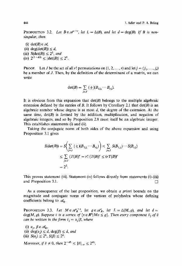
PROPOSITION 3.2. Let B e ~ r r+r, let L = L ( B ) , and let d--- deg(B). I f B is non- singular, then

(i) det(B) ~ d , (ii) deg(det(B)) < d,

(iii) S(det(B)) _< 2 z, and (iv) 2 (a-d)L < ]det(B)l < 2 L.

PROOF. Let J be the set of all r! permutations on (1, 2 , . . . , r) and let j = (Jl,-. . ,Jr) be a member of J. Then, by the definition of the determinant of a matrix, we can write

det(B) = ~ (++_)(Blj,...B~j). jeJ

It is obvious from this expansion that det(B) belongs to the multiple algebraic extension defined by the entries of B. It follows by Corollary 2.1 that det(B) is an algebraic number whose degree is at most d, the degree of the extension. At the same time, det(B) is formed by the addition, multiplication, and negation of algebraic integers, and so by Proposition 2.8 must itself be an algebraic integer. This establishes statements (i) and (ii).

Taking the conjugate norm of both sides of the above expansion and using Proposition 3.1 gives

<_ ~ (T(B))" = r! (T(B)) ~ <_ (rT(B))* jGJ

2 L.

This proves statement (iii). Statement (iv) follows directly from statements (i)-(iii) and Proposition 3.1. []

As a consequence of the last proposition, we obtain a priori bounds on the magnitude and conjugate norm of the vertices of polyhedra whose defining coefficients belong to dR.

PROPOSITION 3.3. Let M e t i e r • let g ed~R, let L = L(M,g), and let d = deg(M, g). Suppose ~ is a vertex o f { v e R b [ M y <_ g}. Then every component ~j of g can be written in the form ~j = ctj/fl, where

(i) ~j,/~ e dR, (ii) deg(~j) _< d, deg(fl) < d, and

(iii) S(~j) <_ 2 L, S(fl) <_ 2 z.

Moreover, if ~ v~ 0, then 2 -aL <_ []~[]~ < 2 dL.

Polynomial Algorithms for Linear Programming over the Algebraic Numbers 445

PROOF. The statement follows trivially from Proposition 3.2 and Cramer's rule. []

Propositions 3.1-3.3 constitute our basic analytical tools. Using them we can modify almost any variant of the ellipsoid method ['8] or the interior-point method [7] to solve problem (P) in time polynomial in its dimension, degree, and conjugate size. In the remaining part of this section we present and analyze an algorithm that is centered on the ellipsoid method. We loosely follow an analysis given by Papadimitriou and Steiglitz [15] for problems with rational data.

For the purposes of the complexity analysis, we assume that we have a machine that performs addition, subtraction, multiplication, division, and comparison of real numbers in constant time per operation. We refer to this model as the real-number model of computation and to algorithms derived under it as real-number algorithms. (See ['4] for a treatment of the theory of general computation over the real numbers.)

We assume that the input of an instance of the LP (P) consists of the following items:

(i) A ~ d ~ • b ~ d ~ , c ~ d ~ . (ii) deg(A, b, c).

(iii) L(A, b, c).

Following the usual conventions, we say that an algorithm solves the LP (P) if, for every problem instance, the algorithm gives us as appropriate: a report that the instance is infeasible, a report that the instance is unbounded, or optimal solutions to both the instance and its dual problem.

Our strategy for demonstrating the polynomial-time solvability of (P) is to establish a chain of polynomial problem equivalencies leading from (P) to problems that can be solved by the ellipsoid method in polynomial time. It should be noted that we have chosen the particulars of this strategy with an eye toward simplicity and ease of understanding, and not the best complexity bounds. Indeed, we are content in showing that the overall procedure is polynomial without deriving the specific form of tl~e polynomial. We conduct our tactics in the same spirit. When it is necessary to have a specific bound on a quantity--such as the conjugate size of a system of inequalities or the volume of polyhedral set--we often settle for one that is easy to obtain, even if additional work would give a tighter or, perhaps, prettier one.

We begin by noting that, given the duality theorem of linear programming, solving the LP (P) is no harder than solving a set of linear dosed inequalities. As a matter of language, we say an algorithm solves a system of inequalities if it gives us a report that the instance is infeasible or a feasible solution to the instance, as appropriate.

PROPOSITION 3.4. Let M ~ ~r • with full column rank, let g ~ d~R, and let 6, 2 ~ R be such that deg(M, g) <_ 6 and L(M, g) <_ 2. Suppose a real-number algorithm exists that, given M, g, 3, and 2, solves My <_ g in time polynomial in r, 6, and )~. Then a

446 I. Adler and P. A. Beling

real-number algorithm exists that solves the LP (P) in time polynomial in m, deg(A, b, c), and L(A, b, c).

PROOF. We outline the desired algorithm for problem (P), using the hypothesized algorithm for linear closed inequalities as a subroutine. We first check the feasibility of (P) by using the subroutine to solve Ax < b. Since the row dimension, degree, and conjugate size of this system are individually bounded from above by the corresponding quantities associated with (P), this step is clearly polynomial in m, deg(A, b, c), and L(A, b, c). If Ax <_ b is infeasible, then we report (P) is infeasible. Otherwise, we use the subroutine to solve the following system:

(P-D) bTy -- cTx <_ 0,

Ax <_b,

ATy < c, - A ~ y < --c, - y <_ O.

Let l denote the row dimension, let d denote the degree, and let L denote the conjugate size of (P-D). Then it is straightforward to establish that l < 5m, d = deg(A, b, c), and L < 4L(A, b, c). It follows that we can use the subroutine to solve (P-D) in time polynomial in m, deg(A, b, c), and L(A, b, c). If (P-D) is infeasible, then we report that (P) is unbounded. Otherwise, we know by duality theory that the pair of vectors, say (~, p), feasible to (P-D) and returned by the subroutine constitute an optimal pair of solutions for (P) and its dual. []

Note that in the last proposition we have suppressed the dependence of the complexity bound on the column dimension of the problem. The assumption that the problem has full column rank technically (although perhaps not aesthetically) justifies this simplification.

Next we note that we can solve a system of linear closed inequalities by solving a closely related system of linear open inequalities.

PROPOSITION 3.5. Let M e d~R • ~ with full column rank, let g ~ d ~ , let L = L(M, #), and let d = deg(M, g). Let e, denote the r-vector of all ones. Then the open system 22dLMv < 22dLg q- e, is feasible if and only if the closed system My < 9 is feasible. Moreover, a real-number algorithm exists that, given a solution to one system, finds a solution to the other system in time polynomial in r.

PROOF. The proof is an adaptation of that given by Papadimitriou and Steiglitz [15, Lemma 8.7, pp. 173-174] for an analogous result concerning systems with rational coefficients. The main difference lies in the use of the properties of conjugate norm (Proposition 3.1) to derive lower bounds on polynomial forms involving algebraic integers. A similar adaptation is shown in detail in [1]. []

PROPOSITION 3.6. Let M e t i e r +s, let g e d~R, and let K = {v e RSlMv < g}. Let R 1 be a real number such that Itvlj~o <- R1 for all v~K. Let R2, 0 < R 2 ~_ 1, be a real

Polynomial Algorithms for Linear Programming over the Algebraic Numbers 447

number such that if K ~ (2~, then the s-dimensional volume of g satisfies vol~(K) ~ R 2 .

Then a real-number algorithm, called the ellipsoid method, exists that, 9iven M, 9, R1, R2, either finds ~ ~ K or (correctly) asserts that K is empty. Moreover, the number of arithmetic operations performed by the algorithm is polynomial in r and log(R1/ R2).

PROOF. The ellipsoid method is well-studied in most recent texts on combinator- ial optimization or linear programming. One technical point deserves special mention, however.

In its basic form, the ellipsoid method requires exact calculation of square roots, something that cannot be achieved under either a rational-number model of computation or the real-number model that we use in this paper (see [20] for a real-number model that explicitly includes the square-root operation). Under a rational-number model this difficulty can be sidestepped by using a finite-precision variant of the ellipsoid method (see, e.g., [5] or [15]) in conjunction with a subroutine (based, say, on Newton's method) for approximating square roots. It is straightforward to show that the same approach works in our case. []

We require one more preliminary result before we can prove the main result of the section.

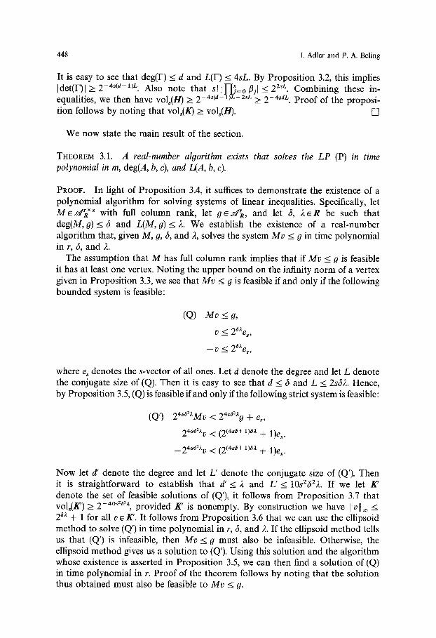
PROPOSITION 3.7. Let M ~ d~R • ~, let 9 ~ d ~ , let L = L(M, g), and let d = deg(M, 9). Let K = {v~R~[Mv < 9}. Then if K is bounded and nonempty the s-dimensional volume of K satisfies vol~(K) _> 2 -4~dL.

PROOF. The proof is an adaptation of a standard proof given for the analogous result concerning systems with rational coefficients (see [5] or [15]).

Suppose K is bounded and nonempty. Then since it has an interior and is bounded, the polyhedral set g = {v e R q M v < 9} has s + 1 affinely independent vertices, say v ~ . . . . . v ~. Let H denote the convex hull of v ~ . . . . . v ~. Since H is a simplex, its s-dimensional volume is given by a well-known formula:

[:ol l l v o l ~ ( H ) = ~ det vl ... v s .

By Proposition 3.3, each component v~ of vertex v a can be written as ~ = O~j,k/flj , where S(aj, k) < 2 L and S(flj) <_ 2 L. Rewriting the volume equation, we have

vols(H) - Idet(F) t, IIl :o

where the matrix F is defined as

L~o,~ ~,,~ "'~ ~,~/

448 I. Adler and P. A. Beling

It is easy to see that deg(F) < d and L(F) < 4sL. By Proposition 3.2, this implies [det(F)l > 2 -4s(d-1)L. Also note that s! II-[~=o/~jl-< 2 2sL. Combining these in- equalities, we then have vol~(H) > 2-4~(a-1)L-2~L > 2-4~dL. Proof of the proposi- tion follows by noting that vol,(K) > vols(H). []

We now state the main result of the section.

THEOREM 3.1. A real-number algorithm exists that solves the LP (P) in time polynomial in m, deg(A, b, c), and L(A, b, c).

PROOF. In light of Proposition 3.4, it suffices to demonstrate the existence of a polynomial algorithm for solving systems of linear inequalities. Specifically, let M e d ~ • with full column rank, let g ~ ~r and let 5, 2 ~ R be such that deg(M, g)-< 3 and L(M, g) < 2. We establish the existence of a real-number algorithm that, given M, g, 3, and 2, solves the system My <_ g in time polynomial in r, 3, and 2.

The assumption that M has full column rank implies that if My <_ g is feasible it has at least one vertex. Noting the upper bound on the infinity norm of a vertex given in Proposition 3.3, we see that My <_ g is feasible if and only if the following bounded system is feasible:

(Q) My < g,

v < 2~e~,

--v _< 2~%s,

where e~ denotes the s-vector of all ones. Let d denote the degree and let L denote the conjugate size of (Q). Then it is easy to see that d < 5 and L < 2s32. Hence, by Proposition 3.5, (Q) is feasible if and only if the following strict system is feasible:

(Q') 24s~2~Mv < 24s~ + e ,

24so2,t v < (2(4s0+ 1)0x + 1)e~,

__24sa22 v < (2(4s6+ 1)aa + 1)e,.

Now let d' denote the degree and let L' denote the conjugate size of (Q'). Then it is straightforward to establish that d ' < 2 and L'<_ 10s2322. If we let K' denote the set of feasible solutions of (Q'), it follows from Proposition 3.7 that vols(K') >_ 2 -4~ provided K' is nonempty. By construction we have I[vN~o < 2 ez + 1 for all v e K'. It follows from Proposition 3.6 that we can use the ellipsoid method to solve (Q') in time polynomial in r, 6, and 2. If the ellipsoid method tells us that (Q') is infeasible, then My < g must also be infeasible. Otherwise, the ellipsoid method gives us a solution to (Q'). Using this solution and the algorithm whose existence is asserted in Proposition 3.5, we can then find a solution of (Q) in time polynomial in r. Proof of the theorem follows by noting that the solution thus obtained must also be feasible to My < g.

Polynomial Algorithms for Linear Programming over the Algebraic Numbers 449

4. Extensions to Other Input Models. The complexity bounds for linear pro- gramming developed in the last section are stated in terms of problem degree and conjugate size. Although these quantities are generally not an explicit part of an LP, they can often be deduced given some limited a p r i o r i information about the individual problem coefficients. In this section we discuss ways of obtaining bounds on problem degree and conjugate size under several different assumptions about the form of the problem coefficients. Because it is impossible to anticipate every input form, the discussion is more illustrative than exhaustive. We begin by working through an example in which the problem degree and conjugate size, although not apparent from the given data, are easy to bound. The nature of this analysis leads us to consider some results from number theory that serve as useful tools for obtaining bounds for other input forms. We then consider several examples that illustrate the use of these results. We conclude the section by showing how our complexity bounds generalize from the algebraic integers to the algebraic numbers.

Throughout this section we use d to denote the degree and L to denote the conjugate size of (P); that is

d = deg(A, b, c),

L = L ( A , b, c).

Additionally, we use qJ to denote the set of all entries in A, b, and c.

EXAMPLE 4.1. For every �9 ~ qJ, suppose that, in addition to the actual numerical value of ~, we know a set of four integers Zo, zl, z2, z 3 such that ~ =

ao + + + Our first goal is to bound the problem conjugate size, L, by a function of the

quantities available to us. As it turns out, a useful input measure for this purpose is the total number of bits in a binary representation of the integers that define the members of ~P in terms of the square roots. We use E to denote this number.

Recall that L is a nondecreasing function of S(~), ~ ~ ~g. Hence, we may first bound the conjugate norms of the individual input coefficients and then calculate a bound on L from these quantities. Proceeding along these lines, we note that if

= Z 0 -~- Z1N ~ ~- Z2N//3 -~ Z3N//6, then by the properties of the conjugate norm (Proposition 3.1) we have

S(o~) : S(z 0 -q- z i N//2 --[- z2N/~ -q- z3N//6)

-< Izol + [Zx IS(x//~) + Iz2[S(x//~) + Iz31SK/~).

The problem of bounding L is thus reduced to that of finding (or bounding) the conjugate norms of the square-root terms.

Let p be a positive integer such that p is not the square of another integer, it

is easy to show that F(t ) = t 2 - p is the minimal polynomial of x/P- It follows that

450 I. Adler and P. A. Beling

the conjugates of x/P are ~ and -x//p. Hence, we have

S(x/P) = max{Ix//Pl, I - x / P l } = ,,fP.

Substitution in our earlier inequality then gives

s(~) ~ Izol + I z l l ~ + Iz=l~/3 + Izal~,

which holds for any ~ E q?. Using this bound in the formula that defines L, it is straightforward to show that L < mE.

It remains for us to bound d, the degree of (P). First note that, by the definition of the degree of an LP, d equals the degree of the multiple algebraic extension Q(W). It is obvious from the form of the problem coefficients that every e e qJ also

belongs to Q(x//2, x/~, x//-6). This implies Q(q0 c Q(x//2, x//3, x/~). It follows from

Corollary 2.1 that d is no larger than the degree of Q(x/~, x/~, v/6). Letting denote this last quantity and using Proposition 2.5, we then have

d < d < (deg(x/2))(deg(x/~))(deg(x~))

= 8,

where we have used the fact that deg(x/~ ) = deg(x//3) = deg(x/~ ) = 2. Actually, we can tighten the bound on d somewhat by noting that, since

(,e/2)(,45) = ,f6, the extensions 0(,f2, ,/5, ~/~)and 0(,f2, ,f3)are, in fact, the same, and so must have the same degree. Hence we have d ___ 4. Although insignificant in this simple example, the savings from observations of this kind can sometimes be quite dramatic (see Example 4.2).

As a final observation we note that, based on our bounds for d and L, Theorem 3.1 implies that (P) can be solved in time polynomial in m and E.

The ad hoc analysis given in Example 4.1 illustrates an effective strategy for many input forms. To bound L, we first bound S(c~) for each ct e W. If we know a representation for ct in terms of other algebraic integers, we use the properties of the conjugate norm to reduce the problem to that of bounding the conjugate norm of those algebraic integers. To bound d, we identify a set of algebraic numbers-- hopefully smaller than W itself--such that the multiple algebraic extension gen- erated by these numbers includes Q(W). We can then claim that d is at most the product of the degrees of these algebraic integers.

The input form considered in Example 4.1 is a special case of the form ~ = ~ zjOj, where zj is an integer and 0j is an algebraic integer. It is clear that in order to use the general approach outlined above to find bounds for problems with this form we must know something about the degree and conjugate norm of 0. This reflects a general caveat; in any attempt to bound the degree and conjugate size of an LP, we ultimately reach a point where we must bound the degree and conjugate

Polynomial Algorithms for Linear Programming over the Algebraic Numbers 451

norm of an individual algebraic integer. Therefore, it is worth considering how to obtain these bounds from the auxiliary information commonly associated with an algebraic integer.

We begin along these lines by introducing some additional terminology concern- ing polynomials and algebraic integers.

DEFINITION. Let F(t) = zatd q - " " + Z l t q-Z o be a polynomial with coefficients zo, . . . , z a ~ Z. We define the heioht o f the polynomial F to be max j{ J zjJ }. We define the heioht o f an aloebraic integer to be the height of its minimal polynomial.

Next we state a well-known result from the theory of transcendental numbers that relates the conjugate norm of an algebraic integer to its height.

PROPOSITION 4.1. Let ~ be an algebraic integer o f height h. Then S(ct) < 2h.

See, e.g., [17] for proof of Proposition 4.1. The minimal polynomial often contains more information than we need for the

purpose of bounding the degree and height of an algebraic integer. Indeed, it suffices to know the degree and height of any monic, integral polynomial of which the algebraic integer is a root, as the following proposition shows.

PROPOSITION 4.2. Let F be a monic polynomial with integer coefficients, degree l, and height h. Then every root o f F is an algebraic integer o f degree at most l and height at most 4th.

See [13] for a statement and proof of a generalization of Proposition 4.2. As an illustration of the use of the preceding results, we next obtain bounds for

an input form that arises in the theory of LPs whose coefficient matrices are circulant.

EXAMPLE 4.2. Let co be the first primitive pth root of unity; that is,

CO = e 2~i/p, where i = ~ - 1 and p is integer.

In addition to q~, suppose that we know the following:

p - 1 (i) A positive integer p such that every e s W can be written as e = ~j=o zj coi for integers z o , . . . , Zp_ 1.

p--1 (ii) For every e e W, a set of integers z o . . . . . zp_ 1 such that ~ = ~j=o zj mj.

Let E denote the total number of bits in a binary representation of the integers zj in (ii) above.

452 I. Adler and P. A. Beling

We begin by finding a bound on the conjugate norm of each member of ~P. If p - 1 (~ : Z j = O ZjO.) j, then we have

p - 1

_< I z /s(o;) . j=O

We now concentrate on bounding S(co;) for all j ~ {0 . . . . , p - 1}. First note that since ~o jp = 1 for all j = 0 . . . . . p - 1, it is clear that r is a root of the polynomial F ( t ) = t p - 1. Although F is not the minimal polynomial of co j, it does give us enough information to bound S(o/). In particular, since F has degree p and height 1, Proposition 4.2 implies that co j has height at most 4 p. Proposition 4.1 then gives S(~o j) < 4p+ 1, which in turn gives

p - 1

s(a) _< 4v+ F z/ . j=O

Using this last bound it is easy to show that L < 3 m E .

To bound d, note that Q(W) c Q(a~), and so d < deg(r However, 09 is a root of g ( t ) = t p - - 1 and so by Proposition 4.2 has degree at most p. Hence we have d < p. (In fact, it is possible to sharpen our bounds on L and d somewhat by using additional results from number theory concerning the roots of unity.)

Combining our bounds on d and L with Theorem 3.1, we see that (P) can be solved in time polynomial in m, p, and E.

LPs of the form considered in Example 4.2 are analyzed in a different manner but with similar results in [1].

As a further illustration of the use of Propositions 4.1 and 4.2, we consider the following generalization of Example 4.1.

EXAMPLE 4.3. In addition to W, suppose that we know the following:

(i) Positive integers P l . . . . , Pk and 11,..., I k such that every c~ ~ q? can be written

as ct = ~sk.= 1 Zj tJV/~j, for integers z~ . . . . . Zk.

(ii) For every ~ ~ W, a set of integers za . . . . . z k such that ~ -- ~k= 1 Z j ~ .

Let E denote the total number of bits in a binary representation of the integers pj in (i) and zj in (ii) above.

As in the previous examples, we begin by finding a bound on the conjugate

norm of each member of W. If ~ = ~k= 1 Z j ~ , then we have

k

_< Z I zjlS( ). j = l

Now note that ~ is a root of the polynomial F l ( t ) = t lj - p j . Since Fj has degree

lj and height p j, Proposition 4.2 implies that ~ has height at most 4tjpj. It

Polynomial Algorithms for Linear Programming over the Algebraic Numbers 453

follows by Proposition 4.1 that S ( ~ ) < 4~J+lpj. Using this last result and our inequality for S(~), we can easily show that L <<_ m(E + 2 ~k= 1 l j).

To bound d, we first note that Q(W) c Q({ tj~j}). By Proposition 2.1 the degree

of the multiple algebraic extension Q({ tJx/%j})is at most I-[~= 1 d e g ( ~ ) . It follows that d < l-[k=1 deg(tJ~j). However, ~ is a root of F j ( t ) = t t~ - pj, and so by Proposition 4.2 has degree at most lj. Hence we have d < l--Ik= 1 l~.

Combining our bounds on d and L with Theorem 3.1, we see that (P) can be solved in time polynomial in m, I-[k= 1 1i, and E.

We next consider LPs in which we have direct knowledge of the minimal polynomial of each algebraic integer in the problem.

EXAMPLE 4.4. For every a ~ W, suppose that we know both the numerical value of ~ and the minimal polynomial of ~.

Let 5 = I-L~v deg(~), the product of the degrees of the minimal polynomials associated with the members of qJ. Also, let E denote the total number of bits in a binary representation of the coefficients of these polynomials.

Using Proposition 4.1, it is straightforward to show that L is bounded from above by E, the problem-encoding size. To bound d, we again appeal to Proposi- tion 2.5, which states that the degree of a multiple algebraic extension is at most the product of the degrees of the algebraic numbers that define the extension. Since 5 is precisely this last quantity, we have d < d.

Using Theorem 3.1 and our bounds on d and L, we see that (P) can be solved in time polynomial in m, d, and E.

As a final example, we consider an obvious generalization of Example 4.4.

EXAMPLE 4.5. For every a ~ ~ , suppose that we know both the numerical value of a and a monic polynomial F with integer coefficients such that F(a) = 0.

Let 5 denote the product of the degrees of the above polynomials, and let E denote the total number of bits in a binary representation of their coefficients.

Here we can use Proposition 4.2 to bound the degree and height of each a ~ by a function of the degree and height of its associated polynomial. We can then find bounds on d and L precisely as in Example 4.4. Using these bounds, we can then show that (P) can be solved in time polynomial in m, d, and E.

Up to this point we have dealt only with LPs whose coefficients are algebraic integers. We now consider how our complexity results for such problems can be extended to problems with coefficients from the full set of algebraic numbers. Specifically, we show that, given an appropriate description of the problem, we can polynomially transform an LP whose coefficients are algebraic numbers into an equivalent problem whose coefficients are algebraic integers. In both form and effect, this transformation is analogous to the obvious way of turning a problem with rational coefficients into one with integer coefficients--namely multiplication by a common denominator.

454 I. Adler and P. A. Beling

We first consider a way of transforming a single algebraic number into an algebraic integer.

PROPOSITION 4.3. L e t H(t) = t a --k qd - I ta- 1 -F "'" q- qi t + qo be a polynomial wi th

coefficients qo, . . . , qd- 1 ~ Q, and let z be a common denominator f o r qo, . . . , qa- r

Then i f ~ is a root o f H , the product z~ is a root o f

F(t) = t d d- z q d _ l t d -1 q- "'" d- z a - l q l t + zaqo .

Moreover , the coefficients o f F are all integers.

PROOF. Trivial. []

Note that since F is a monic polynomial with integer coefficients, the product za in Proposition 4.3 must be an algebraic integer. It is less obvious but also true that the degree of za is the same as the degree of a.

We next show how to use Proposition 4.3 and our earlier complexity results to bound the complexity of LPs whose coefficients are algebraic numbers. Specifically, we consider an LP whose structure is the same as that of problem (P), but whose coefficients may be algebraic numbers. We use (P') to denoe this problem, and to denote the set of all its coefficients.

To analyze (P') we must work in the Context of a specific input model. We choose for this purpose a model based on Example 4.5. Other input models can be handled in a similar fashion.

For each ~ in the coefficient set ~g, we assume that we know both the numerical value of a and a monic polynomial H with rational coefficients such that H(a) = 0. As in Example 4.5, we let d denote the product of the degrees of these polynomials, and we let E denote the total number of bits in a binary encoding of their coefficients.

Let ~ denote the product of the denominators of the rational numbers that define the polynomials associated with the elements of ~. Then we see from Proposition 4.3 that, for every ~ ~g, the product ~ct is an algebraic integer. Moreover, we know that if a is a root of the polynomial

H( t ) = t a + q d _ i t d -1 q- "'" + q l t q- qo,

then ~ is a root of F(t) = t a + ~qa_i ta-1 + "" + ~a - lqa t + ~aqo. We also know that the coefficients of F are all integers. It follows that by multiplying each element of �9 by ~ and constructing the associated polynomial F we obtain a problem that is precisely in the form of Example 4.5. We call the problem constructed in this manner (P"). Note that we can construct (P") from (P') in time polynomial in m, d, and E.

It is clear that the degree of (P") is no larger than the degree of (P') (in fact, they are equal). Also, it is straightforward to show that the number of bits in a binary encoding of the polynomials in (P") is bounded by a polynomial in m and E.

Polynomial Algorithms for Linear Programming over the Algebraic Numbers 455

Combining these facts with the results in Example 4.5, we see that (P")--and hence (P')--can be solved in time polynomial in m, d, and E.

5. Remarks. 1. The complexity bounds given in this paper are derived under a model of computation that allows real-number input and arithmetic. In fact, this assumption is stronger than necessary. Essentially the same results can be achieved under a rational-number model of computation by using a well-known scheme for the symbolic manipulation of algebraic numbers in conjunction with the results of Section 3. We provide an outline of such a procedure below, but defer a full exposition of the (somewhat messy) details to a subsequent paper [21.

Recall from Proposition 2.4 that the conjugates of an algebraic number are distinct. It follows that if ~ is a real algebraic number with minimal polynomial G, an interval with rational endpoints, say I-q1, q21, exists that contains ~ but does not contain any other root of G. Since the triplet (G; ql, qa) unambiguously defines ct, we can represent ~ in a rational-number machine by storing ql, q2, and the coefficients of G. It can be shown that the roots of G are sufficiently small and well-separated that an isolating interval exists whose binary-encoding size is polynomial in the binary-encoding size of the coefficients of G.

To be useful as part of a linear programming algorithm, the triplet scheme must allow us to manipulate algebraic numbers as well as to represent them. It follows from some results of Lovasz [91, that, given triplets for two algebraic numbers, we can find a triplet that represents their sum, difference, product, or quotient in time polynomial in the encoding lengths of the given triplets. We can also compare two triplets in polynomial time.

Equipped with a means of representing and manipulating algebraic numbers, we can establish the polynomial-time solvability of linear programming in much the same manner as is done in this paper. An unavoidable extra complication of working with a rational-number model of computation is that we must be careful to control the bit size of the rational numbers that occur during the course of the linear programming algorithm. We can do this by using some approximation techniques in conjunction with a well-known finite precision variant of the ellipsoid method. The running time of the overall procedure is polynomial in the problem dimension, problem degree, and the bit size of triplets that represent the input coefficients.

2. Using the basic analytical tools presented in Section 3, the algorithm for combinatorial LPs given by Tardos 1-19] can be modified so that it works with LPs whose coefficients are algebraic integers. As in the rational case, the running time of the resulting algorithm is independent of the data in the objective and right-hand side. The details of this extension are given in [3]. Similar ideas are used in [11, where Tardos's scheme is extended from the rationals to the cyclotomic integers.

We also note that it may be possible to make a similar extension to the algorithm of Norton et al. 1-14], which solves LPs in time independent of the data in a fixed number of rows or columns of the coefficient matrix.

3. In [1] it is shown that standard form LPs with circulant coefficient matrices

456 I. Adler and P. A. Beling

can be solved in strongly polynomial time. The key idea behind this result is a transformation of the given problem into an equivalent problem in which the entries of the coefficient matrix belong to the subring of the algebraic integers discussed in Example 4.2 and have small conjugate norm. This transformation is accomplished by multiplying the equality constraints by the pseudoinverse of the coefficient matrix. The transformed problem can then be solved in strongly polynomial time using a variant of the Tardos scheme (see the previous remark) in conjunction with a polynomial-time algorithm for LPs whose coefficients belong to the subring.

In light of the results in this paper, which extend the linear programming results in [1] to general algebraic numbers, it is worth investigating whether other classes of problems can be shown to be strongly polynomial by arguments similar to those used for circulant LPs. Equivalently, we can ask whether there are other simultaneously diagonalizable families of matrices whose diagonalizing matrix is composed of small algebraic numbers (not necessarily from the subring in [1]). Indeed, it appears that such families do exist and that considerable progress in identifying them can be made by using results from the theory of group representa- tions. We plan to report on this topic in a subsequent paper.

Acknowledgments. We thank Leonid Khachiyan, Uriel Rothblum, and Ron Shamir for valuable discussions on extending our earlier work with cyclotomic integers to the present case. We are also indebted to Michael Todd for perceptive comments about the generalization from algebraic integers to algebraic numbers.

References

[1] I. Adler and P. A. Beling, Polynomial Algorithms for LP over a Subring of the Algebraic Integers with Applications to LP with Circulant Matrices, Mathematical Programming 57 (1992), 121-143.

[2] I. Adler and P. A. Beling, Turing Algorithms for Linear Programming over the Algebraic Numbers, manuscript, September, 1992.

1-3] P.A. Beling, Linear Programming~over the Algebraic Numbers, Ph.D. dissertation, University of California, Berkeley, 1991.

I-4] L. Blum, M. Shub, and S. Smale, On a Theory of Computation and Complexity over the Real Numbers; NP-completeness, Recursive Functions and Universal Machines, Bulletin of the AMS 21(1) (1989), 1-46.

[5] M. Grotschel, L. Lovasz, and A. Schrijver, Geometric Algorithms and Combinatorial Optimiza- tion, Springer-Verlag, Berlin, 1988.

[6] K. Ireland and M. Rosen, A Classical Introduction to modern Number Theory, Springer-Verlag, New York, 1972.

[7] N. Karmarkar, A New Polynomial Time Algorithm for Linear Programming, Combinatorica 4 (1984), 373-395.

1-8] L. Khachiyan, A Polynomial Algorithm in Linear Programming, Soviet Mathematics Doklady 20 (1979), 191-194.

[9] L. Lovasz, An Algorithmic Theory of Numbers, Graphs and Covexity, Society for Industrial and Applied Mathematics, Philadelphia, PA, 1986.

[10] N. Megiddo, Towards a Genuinely Polynomial Algorithm for Linear Programming, SIAM Journal on Computing 12(2) (1983), 347-353.

Polynomial Algorithms for Linear Programming over the Algebraic Numbers 457

[11] N. Megiddo, Linear Programming in Linear Time when the Dimension is Fixed, Journal of the Association for Computing Machinery 31 (1984), 114-127.

[12] N. Megiddo, On Solving the Linear Programming Problem Approximately, Contemporary mathematics, Vol. 114, The American Mathematical Society, Providence, RI, 1990, pp. 35-50.

[13] M. Mignotte, Some Useful Bounds, in: B. Buchberger, G. E. Collins, and R. Loos (eds.), Computer Algebra, Springer-Verlag, Wien, 1983, pp. 259-263.

[14] C. Norton, S. Plotkin, and E. Tardos, using Separation Algorithms in Fixed Dimension, Proceedings of the 1st ACM/SIAM Symposium on Discrete Algorithms, 1990, pp. 377-387.

[15] C.H. Papadimitriou and K. Steiglitz, Combinatorial Optimization, Prentice-Hall, Englewood Cliffs, NJ, 1982.

[16] H. Pollard and H. G. Diamond, The Theory of Algebraic numbers, 2rid edn., The Mathematical Association of America, Washington, DC, 1975.

[17] A.B. Shidlovskii, Transcendental Numbers, de Gruyter, Berlin, 1989. [18] I.N. Stewart and D. O. Tall, Algebraic Number Theory, Chapman & Hall, New York, 1987. [19] E. Tardos, A Strongly Polynomial Algorithm To Solve Combinatorial Linear Programs,

Opterations Research 34 (1986), 250-256. [20] J.F. Traub and H. Wozniakowski, Complexity of Linear Programming, Operations Research

Letters 1 (1982), 59-62.