Polynomial Optimization: Structures, Algorithms, and ...

Polynomial Optimization: Structures, Algorithms, andEngineering Applications

A DISSERTATION

SUBMITTED TO THE FACULTY OF THE GRADUATE SCHOOL

OF THE UNIVERSITY OF MINNESOTA

BY

BO JIANG

IN PARTIAL FULFILLMENT OF THE REQUIREMENTS

FOR THE DEGREE OF

DOCTOR OF PHILOSOPHY

SHUZHONG ZHANG

August, 2013

c© BO JIANG 2013

ALL RIGHTS RESERVED

Acknowledgements

I am deeply indebted to my advisor Professor Shuzhong Zhang, who brought me into

serval interesting research topics, and has provided me constant supports and encourage-

ments. Thanks to him, I had the great fortune to start my Ph.D. study at the Chinese

University of Hong Kong (CUHK), and then continued to complete the whole Ph.D.

program at the University of Minnesota. I have learned a lot from him. In particular,

I am greatly inspired by his never-ending passion to understand how things work in a

deep way, which, on several occasions, pushed me toward the direction leading to the

beautiful results that I would not have expected before.

I would like to express my sincere gratitude to the members of my thesis committee,

Professors Bill Cooper, John Carlsson and Zhi-Quan (Tom) Luo, for their careful reading

and valuable comments on my dissertation. I would not have a smooth transition

from CUHK to University of Minnesota, if I did not receive the strong support and

help from Bill. I have learned a lot on the computational geometry and the algorithm

design techniques in optimization from the two group discussions led by John and Tom

respectively.

My gratitude extends to my other collaborators: Shiqian Ma, Zhening Li, Simai He,

Augusto Aubry, and Antonio De Maio. The numerous fruitful discussions with them

have stimulated a lot of exiting joint works. Especially, I would like to thank Shiqian

and Zhening for their academic insights and career advice, and the email-discussion

with Augusto is a memorable experience.

My officemates and friends in both CUHK and University of Minnesota have made

my study enjoyable. Particularly, I would like to acknowledge the friendship and the

support that I received from: Youfeng Su, Kencheng Wang, Binyang Li, Dakui Wang,

Lanjun Zhou, Bilian Chen, Xiaoguo Wang, Keith Wong, Ke Hou, Yi Yang, Yanyi Yang,

i

Shuang Chen, Yibin Chen, Chenhao Du, Yan Liu, and Fan Jia.

I am greatly indebted to my parents, Shujie Zhang and Ligui Jiang, who have

always filled my life with unconditional love and support. I would also like to express

my deepest gratitude to my wife, Liu Yang, for her company and support throughout

my Ph.D. study.

This dissertation is devoted in part to my mentor, Professor Xuexiang Huang, at

Fundan University. I may never start research on optimization and pursue the Ph.D.

degree if I did not meet him. It has been almost ten months since his passing away. I

hope he could be proud of my academic achievement should he still be around to read

this thesis.

ii

Dedication

This work is dedicated to my parents and to Professor Xuexiang Huang.

iii

Abstract

As a fundamental model in Operations Research, polynomial optimization has been

receiving increasingly more attention in the recent years, due to its versatile modern

applications in engineering such as biomedical engineering, signal processing, mate-

rial science, speech recognition, and so on. In this thesis, we present a systematic

study of polynomial optimization. First, we study the structures of various polyno-

mial functions, based on which efficient algorithms will consequently be developed. The

newly developed solution methods will be tested on a variety of engineering applications.

Specifically, we first study the class of nonnegative polynomials. Six fundamentally im-

portant types of nonnegative quartic functions coagulating into a chain in decreasing

order will be presented. This structure is useful in understanding the nature of quartic

polynomials. We further consider the polynomial sized representation of a very specific

nonnegative polynomial, and this representation enables us to address an open question

asserting that the computation of the matrix 2 7→ 4 norm is NP-hard in general. Then

we proceed to studying polynomial function in random variables and establish a series of

fundamental probability inequalities. Similar to the relationship between the symmetric

matrices and the quadratic functions, there also exists a one-to-one correspondence be-

tween the super-symmetric tensors and the homogeneous polynomials, and this leads to

the knowledge of tensor related problems. We then proceed to a new notion of matrix-

rank for the even order tensors. Unlike the CP-rank of tensors, the matrix-rank is easy

to compute. On the computational side, the afore-mentioned probability inequalities

lead to new approximation algorithms with better approximation ratios than the ones

known in the literature. We also propose approximation algorithms for polynomial op-

timization in complex variables. At the same time, we consider first order algorithms

such as the alternating direction method of multipliers (ADMM), and the maximum

block improvement algorithms (MBI). Finally, we test the new algorithms by solving

real engineering problems including the tensor PCA problem, the tensor recovery prob-

lem in computer vision and the radar waveform design problem. Excellent performances

of the proposed methods have been confirmed by our numerical results.

iv

Contents

Acknowledgements i

Dedication iii

Abstract iv

List of Tables ix

List of Figures x

1 Introduction 1

1.1 Motivation and Literature Review . . . . . . . . . . . . . . . . . . . . . 1

1.2 Main Contributions and Organization . . . . . . . . . . . . . . . . . . . 6

1.3 Notations and Preliminaries . . . . . . . . . . . . . . . . . . . . . . . . . 9

2 Cones of Nonnegative Quartic Forms 11

2.1 Introduction . . . . . . . . . . . . . . . . . . . . . . . . . . . . . . . . . . 11

2.1.1 Motivation . . . . . . . . . . . . . . . . . . . . . . . . . . . . . . 11

2.1.2 Introducing the Quartic Forms . . . . . . . . . . . . . . . . . . . 13

2.1.3 The Contributions and the Organization . . . . . . . . . . . . . . 17

2.2 Quartic PSD Forms, Quartic SOS Forms, and the Dual Cones . . . . . . 18

2.2.1 Closedness . . . . . . . . . . . . . . . . . . . . . . . . . . . . . . 19

2.2.2 Alternative Representations . . . . . . . . . . . . . . . . . . . . . 20

2.2.3 Duality . . . . . . . . . . . . . . . . . . . . . . . . . . . . . . . . 23

2.2.4 The Hierarchical Structure . . . . . . . . . . . . . . . . . . . . . 25

v

2.3 Cones Related to Convex Quartic Forms . . . . . . . . . . . . . . . . . . 27

2.4 Complexities, Low-Dimensional Cases, and the Interiors of the Quartic

Cones . . . . . . . . . . . . . . . . . . . . . . . . . . . . . . . . . . . . . 30

2.4.1 Complexity . . . . . . . . . . . . . . . . . . . . . . . . . . . . . . 30

2.4.2 The Low Dimensional Cases . . . . . . . . . . . . . . . . . . . . . 35

2.4.3 Interiors of the Cones . . . . . . . . . . . . . . . . . . . . . . . . 36

2.5 Quartic Conic Programming . . . . . . . . . . . . . . . . . . . . . . . . . 39

2.5.1 Quartic Polynomial Optimization . . . . . . . . . . . . . . . . . . 40

2.5.2 Biquadratic Assignment Problems . . . . . . . . . . . . . . . . . 45

2.5.3 Eigenvalues of Fourth Order Super-Symmetric Tensor . . . . . . 46

3 Polynomial Sized Representation of Hilbert’s Identity 48

3.1 Introduction . . . . . . . . . . . . . . . . . . . . . . . . . . . . . . . . . . 48

3.2 k-Wise Zero-Correlation Random Variables . . . . . . . . . . . . . . . . 50

3.3 Construction of k-wise Zero-Correlated Random Variables . . . . . . . . 52

3.3.1 k-wise Regular Sequence . . . . . . . . . . . . . . . . . . . . . . . 53

3.3.2 A Randomized Algorithm . . . . . . . . . . . . . . . . . . . . . . 54

3.3.3 De-Randomization . . . . . . . . . . . . . . . . . . . . . . . . . . 56

3.4 Polynomial-Size Representation of Hilbert’s Identity . . . . . . . . . . . 57

3.4.1 Polynomial-Size Representation of Quartic Hilbert’s Identity . . 57

3.4.2 Polynomial-Size Representation of of qd-th degree Hilbert’s Identity 59

3.5 Matrix q 7→ p Norm Problem . . . . . . . . . . . . . . . . . . . . . . . . 60

4 Matrix-Rank of Even Order Tensors 63

4.1 Introduction . . . . . . . . . . . . . . . . . . . . . . . . . . . . . . . . . . 63

4.2 Some Properties about Strongly Symmetric Matrix Rank . . . . . . . . 67

4.3 Bounding CP Rank through Matrix Rank . . . . . . . . . . . . . . . . . 70

4.4 Rank-One Equivalence between Matrix Rank and Symmetric CP Rank . 73

5 Probability Bounds for Polynomial Functions in

Random Variables 79

5.1 Introduction . . . . . . . . . . . . . . . . . . . . . . . . . . . . . . . . . . 79

5.2 Multilinear Tensor Function in Random Variables . . . . . . . . . . . . . 83

vi

5.2.1 Multilinear Tensor Function in Bernoulli Random Variables . . . 85

5.2.2 Multilinear Tensor Function over Hyperspheres . . . . . . . . . . 88

5.3 Homogeneous Polynomial Function in Random Variables . . . . . . . . . 92

5.4 Proofs of Theorem 5.3.1 and Proposition 5.3.2 . . . . . . . . . . . . . . . 95

6 New Approximation Algorithms for Real Polynomial Optimization 101

6.1 Introduction . . . . . . . . . . . . . . . . . . . . . . . . . . . . . . . . . . 101

6.2 Polynomial Optimization in Binary Variables . . . . . . . . . . . . . . . 103

6.3 Polynomial Optimization over Hyperspheres . . . . . . . . . . . . . . . . 108

6.4 Polynomial Function Mixed Integer Programming . . . . . . . . . . . . . 110

7 Approximation Algorithms for Complex Polynomial Optimization 112

7.1 Introduction . . . . . . . . . . . . . . . . . . . . . . . . . . . . . . . . . . 112

7.2 Complex Multilinear Form Optimization . . . . . . . . . . . . . . . . . . 117

7.2.1 Multilinear Form in the m-th Roots of Unity . . . . . . . . . . . 118

7.2.2 Multilinear Form with Unity Constraints . . . . . . . . . . . . . 121

7.2.3 Multilinear Form with Spherical Constraints . . . . . . . . . . . 123

7.3 Complex Homogeneous Polynomial Optimization . . . . . . . . . . . . . 124

7.3.1 Homogeneous Polynomial in the m-th Roots of Unity . . . . . . 125

7.3.2 Homogeneous Polynomial with Unity Constraints . . . . . . . . . 129

7.3.3 Homogeneous Polynomial with Spherical Constraint . . . . . . . 130

7.4 Necessary and Sufficient Conditions for Real Valued Complex Polynomials132

7.5 Conjugate Form Optimization . . . . . . . . . . . . . . . . . . . . . . . . 137

7.5.1 Conjugate Form in the m-th Roots of Unity . . . . . . . . . . . . 139

7.5.2 Conjugate form with Unity Constraints or Spherical Constraint . 141

8 Tensor Principal Component Analysis via Convex Optimization 143

8.1 Introduction . . . . . . . . . . . . . . . . . . . . . . . . . . . . . . . . . . 143

8.2 A Nuclear Norm Penalty Approach . . . . . . . . . . . . . . . . . . . . . 148

8.3 Semidefinite Programming Relaxation . . . . . . . . . . . . . . . . . . . 151

8.4 Alternating Direction Method of Multipliers . . . . . . . . . . . . . . . . 154

8.4.1 ADMM for Nuclear Penalty Problem (8.13) . . . . . . . . . . . . 155

8.4.2 The Projection . . . . . . . . . . . . . . . . . . . . . . . . . . . . 156

vii

8.4.3 ADMM for SDP Relaxation (8.14) . . . . . . . . . . . . . . . . . 158

8.5 Numerical Results . . . . . . . . . . . . . . . . . . . . . . . . . . . . . . 158

8.5.1 The ADMM for Convex Programs (8.13) and (8.14) . . . . . . . 158

8.5.2 Comparison with SOS and MBI . . . . . . . . . . . . . . . . . . 161

8.6 Extensions . . . . . . . . . . . . . . . . . . . . . . . . . . . . . . . . . . . 163

8.6.1 Biquadratic Tensor PCA . . . . . . . . . . . . . . . . . . . . . . . 164

8.6.2 Trilinear Tensor PCA . . . . . . . . . . . . . . . . . . . . . . . . 165

8.6.3 Quadrilinear Tensor PCA . . . . . . . . . . . . . . . . . . . . . . 166

8.6.4 Even Order Multilinear PCA . . . . . . . . . . . . . . . . . . . . 168

8.6.5 Odd Degree Tensor PCA . . . . . . . . . . . . . . . . . . . . . . 170

9 Low-Rank Tensor Optimization 171

9.1 Introduction . . . . . . . . . . . . . . . . . . . . . . . . . . . . . . . . . . 171

9.2 Optimizing Low-Rank Tensor Problem through Matrix Rank . . . . . . 172

9.3 Numerical Results . . . . . . . . . . . . . . . . . . . . . . . . . . . . . . 174

9.3.1 Synthetic Examples . . . . . . . . . . . . . . . . . . . . . . . . . 174

9.3.2 Example in Color Videos . . . . . . . . . . . . . . . . . . . . . . 175

10 An Application in Radar Waveform Design 178

10.1 Introduction . . . . . . . . . . . . . . . . . . . . . . . . . . . . . . . . . . 178

10.2 Maximum Block Improvement Method . . . . . . . . . . . . . . . . . . 182

10.3 Performance Assessment . . . . . . . . . . . . . . . . . . . . . . . . . . . 191

11 Conclusion and Discussion 195

References 197

viii

List of Tables

7.1 Organization of the chapter and the approximation results . . . . . . . . 117

8.1 Frequency of nuclear norm penalty problem (8.13) having a rank-one

solution . . . . . . . . . . . . . . . . . . . . . . . . . . . . . . . . . . . . 151

8.2 Frequency of SDP relaxation (8.14) having a rank-one solution . . . . . 154

8.3 Comparison of CVX and ADMM for small-scale problems . . . . . . . . 160

8.4 Comparison of CVX and ADMM for large-scale problems . . . . . . . . 161

8.5 Comparison SDP Relaxation by ADMM with GloptiPoly 3 and MBI. . . 163

8.6 Frequency of problem (8.32) having rank-one solution . . . . . . . . . . 165

9.1 CP-rank of original tensor VS matrix-rank of recovered tensor through (9.5)175

ix

List of Figures

2.1 Hierarchy for the cones of quartic forms . . . . . . . . . . . . . . . . . . 34

9.1 Video Completion. The first row are the 3 frames of the original video

sequence. The second row are images with 80% missing data. The last

row are recovered images . . . . . . . . . . . . . . . . . . . . . . . . . . . 176

9.2 Robust Video Recovery. The first row are the 3 frames of the original

video sequence. The second row are recovered background. The last row

are recovered foreground . . . . . . . . . . . . . . . . . . . . . . . . . . . 177

10.1 Range-Doppler inference map . . . . . . . . . . . . . . . . . . . . . . . . 192

10.2 SIR versus N , for the uncoded transmission, the synthesized code, and

the radar codes designed exploiting some λ values. . . . . . . . . . . . . 193

10.3 Ambiguity function, in dB, of the synthesized transmission code s? for

N = 25 (also in fuchsia the assumed interfering regions). . . . . . . . . 194

x

Chapter 1

Introduction

1.1 Motivation and Literature Review

Polynomial optimization is a fundamental model in the field of Operations Research.

Basically, it is to maximize (or minimize) a polynomial objective function, subject to

certain polynomial constraints. Recently this problem has attracted much attention,

due to its widely applications in various engineering problems such as biomedical engi-

neering [1, 2, 3], signal processing [4, 5, 6], material science [7], speech recognition [8].

To motivate our study and illustrate the usefulness of polynomial optimization, we shall

mention a few concrete examples as immediate applications below. For instance, in the

field of biomedical engineering, Ghosh et al. [2] formulated a fiber detection problem in

Diffusion Magnetic Resonance Imaging (MRI) by maximizing a homogenous polynomial

function, subject to a spherical constraint, Zhang et al. [3] proposed a new framework

for co-clustering of gene expression data based on generic multi-linear optimization (a

special case of polynomial optimization) model. There are also many polynomial opti-

mization problems arising from signal processing, see e.g. Maricic et al. [4], a quartic

polynomial model was proposed for blind channel equalization in digital communication,

and in Aittomaki and Koivunen [9] the problem of beampattern synthesis in array sig-

nal processing was formulated as a complex multivariate quartic minimization problem.

Soare, Yoon, and Cazacu [7] proposed some 4th, 6th and 8th order homogeneous poly-

nomials to describe the plastic anisotropy of orthotropic sheet metal, a typical problem

in material sciences.

1

2

As we have seen, it is basically impossible to list, even partially, the successful stories

of polynomial optimization. However, compared with the intensive and extensive study

of quadratic problems, the study of higher order polynomial optimization, even the

quartic model, is quite limited. For example, consider the following query:

given a fourth degree polynomial function in n variables, can one easily tell

if the function is convex or not?

This simple-looking question was first put forward by Shor [10] in 1992, which turned

out later to be a very challenging question to answer. For almost two decades, the

question remained open. Only until recently Ahmadi et al. [11] proved that checking the

convexity of a general quartic polynomial function is actually strongly NP-hard. Notice

that checking the convexity of a quadratic function is an easy problem. Therefore,

their groundbreaking result not only settled this particular open problem, but also

helped to indicate that the study of generic polynomial optimization will be all the

more compelling and interesting.

This Ph.D. thesis aims at approaching polynomial optimization by first studying the

structures of various polynomial functions, and then proposing efficient algorithms to

solve various polynomial optimization models, then finally presenting results of novel

engineering applications via polynomial optimization models.

The first step towards the systematic study on polynomial optimization, of course, is

to understand how the polynomial functions behave. In particular, we shall focus on the

nonnegativity of polynomials, this is because there is an intrinsic connection between

optimizing a polynomial function and the description of all the polynomial functions

that are nonnegative over a given domain. For the case of quadratic polynomials, this

connection was explored by Sturm and Zhang in [12], and later for the bi-quadratic case

in Luo et al. [13]. For higher order polynomial function, historically, such investigations

can be traced back to the 19th century when the relationship between nonnegative poly-

nomial functions and the sum of squares (SOS) of polynomials was explicitly studied.

Hilbert [14] in 1888 showed that the only three classes of polynomial functions where

this is generically true can be explicitly identified: (1) univariate polynomials; (2) mul-

tivariate quadratic polynomials; (3) bivariate quartic polynomials. There are certainly

other interesting classes of nonnegative polynomials. For instance, the convex polyno-

mial functions, and sos-convex polynomials introduced by Helton and Nie [15] can both

3

be categorized into certain kind of nonnegative polynomial.

Besides, a very interesting and specific nonnegative polynomial in the form of

(n∑i=1

x2i

)ddeserves a further investigation. Hilbert showed that this kind of polynomial bears cer-

tain ’rank one’ representation structure. In particular for any fixed positive integers d

and n, there always exist rational vectors a1, a2, ..., at ∈ Rn such that(n∑i=1

x2i

)d=

t∑j=1

((aj)>x

)2d, where x = (x1, x2, · · · , xn) ∈ Rn. (1.1)

For instance, when n = 4 and d = 2, we have

(x21 + x2

2 + x23 + x2

4)2 =1

6

∑1≤i<j≤4

(xi + xj)4 +

1

6

∑1≤i<j≤4

(xi − xj)4,

which is called Liouville’s identity. In the literature, identity (1.1) is often referred to

as Hilbert’s identity, and this identity turns out to be extremely useful. For example,

with the help of (1.1), Reznick [16] managed to prove the following result:

Let p(x) be 2d-th degree homogeneous positive polynomial in n variables.

Then there exists a positive integer r and vectors c1, c2, · · · , ct ∈ Rn such

that

‖x‖2r−2d2 p(x) =

t∑i=1

(c>i x)2r

for all x ∈ Rn.

Reznick’s result above solves Hilbert’s seventeenth problem constructively (albeit only

for the case p(x) is positive definite). Hilbert (see [17]) proved (1.1) constructively,

however, in his construction, the number of 2d powered linear items on the right hand

side is (2d+ 1)n, which is exponential in n. For practical purposes, this representation

is too lengthy. As a matter of fact, by Caratheodory’s theorem [18], one can argue

that in principle there exist no more than(n+2d−1

2d

)items in the expression (1.1).

Unfortunately, Caratheodory’s theorem is non-constructive, and thus an open problem

remains: For fixed d, find a polynomially sized representation for (1.1).

Therefore, conducting a systematic study on the nonnegative polynomials becomes

one of the central topics in this thesis.

4

Besides, we also interested in the probability in the form of

Probξ∼S0

f(ξ) ≥ τ max

x∈Sf(x)

≥ θ, (1.2)

where f(·) is certain polynomial function, τ > 0 and 0 < θ < 1 are certain constants.

This is because that most classical results in probability theory is to upper bound the

tail of a distribution (e.g. the Markov inequality and the Chebyshev inequality), say

Prob ξ ≥ a ≤ b. However, in some applications a lower bound for such probability

can be relevant.

One interesting example is a result due to Ben-Tal, Nemirovskii, and Roos [19],

where they proved a lower bound of 1/8n2 for the probability that a homogeneous

quadratic form of n binary i.i.d. Bernoulli random variables lies above its mean. More

precisely, they proved the following:

Let F ∈ Rn×n be a symmetric matrix and ξ = (ξ1, ξ2, · · · , ξn) be i.i.d.

Bernoulli random variables, each taking values 1 and −1 with equal proba-

bility. Then Prob ξ>Fξ ≥ tr (F ) ≥ 1/8n2.

As a matter of fact, the author went on to conjecture in [19] that the lower bound can

be as high as 1/4, which was very recently disproved by Yuan [20]. However, the exact

universal constant lower bound remains open. A significant progress on this conjecture

is due to He et al. [21], where the authors improved the lower bound of 1/8n2 to 0.03.

Note that the result of He et al. [21] also holds for any ξi’s being i.i.d. standard normal

variables. Luo and Zhang [22] provides a constant lower bound for the probability

that a homogeneous quartic function of a zero mean multi-variate normal distribution

lies above its mean, which was a first attempt to extend such probability bound for

functions of random vector beyond quadratic. Our goal is to establish (1.2) for generic

polynomial.

It is also very helpful to study the various properties of tensors, since there is a one-to-

one mapping from the homogeneous polynomial functions with degree d to the d-th order

super-symmetric tensors (see Section 1.3). Besides, the emergence of multidimensional

data in signal processing, computer vision, medical imaging and machine learning can

also be viewed as tensors. Therefore tensor-based data analysis attracted more and more

research attention. In practice, the underlying tensor often appears to be equipped with

5

some low-rank structure. However, the commonly used tensor CP-rank [23, 24] is hard

to compute [25]. Therefore, in this thesis, we propose the so-called matrix-rank for even

order tensors, and show that this rank is easy to compute and bears many interesting

properties. And this matrix-rank can be further used in the low-rank optimization

problems.

Our second main research focus deals with designing efficient algorithms that solve

particular kinds of polynomial optimization problems; this is already a challenging task.

For example, even the simplest instances of polynomial optimization, such as maximiz-

ing a cubic polynomial over a sphere, is NP-hard (Nesterov [26]). To find the global

optimizer, Lasserre [27, 28] and Parrilo [29, 30] developed an approach called SOS,

however this method has only theoretical appeal, since it needs solving a (possibly

large) Semidefinite Program and in many cases the solver based on SOS method can

merely get a bound (not feasible solution) for the optimal value before it stops. There-

fore, it is natural to ask whether one can design efficient algorithms for a large class

of polynomial optimization problems with provable approximation guarantees. As a

first step towards answering that question, de Klerk et al. [31] considered the prob-

lem of optimizing a fixed degree even form over the sphere and designed a polynomial

time approximation scheme. The problem of optimizing a more general multivariate

polynomial was not addressed until Luo and Zhang [22] designed the first polynomial

time approximation algorithm for optimizing a multivariate quartic polynomial over a

region defined by quadratic inequalities. Sooner afterward, Ling et al. [32] studied a

special quartic optimization model, which is to maximize a bi-quadratic function over

two spherical constraints. Most recently, He, Li and Zhang presented a series of works

on general homogenous (inhomogenous, discrete) polynomial optimization [33, 34, 35].

So [36] reinvestigate sphere constrained homogeneous polynomial problems and propose

a deterministic algorithm with an improved approximation ratio. For a comprehensive

survey on the topic, one may refer to the recent Ph.D. thesis of Li [37].

In case of complex valued polynomial optimization, Ben-Tal, Nemirovski and Roos

[38] first studied complex quadratic optimization model with objective function being

nonnegative by using complex matrix cube theorem. Zhang and Huang [39], So, Zhang

and Ye [40] considered complex quadratic (include conjugate items) problems. After

that Huang and Zhang [41] also considered bi-linear complex optimization problems.

6

However, to the best of our knowledge there is no result in the literature on approxi-

mation algorithms for higher order complex polynomial optimization problems. In this

thesis we also provide various approximation algorithms to complex polynomial opti-

mizations as well as some real valued polynomial optimizations with spherical (binary)

constraints.

1.2 Main Contributions and Organization

This thesis is organized as follows. We shall start our discussion by exploring various

structures of polynomial functions and tensors, which will cover Chapters 2 to 5.

In Chapter 2, we first introduce the definition of six different nonnegative quar-

tic polynomials. Then we shall prove they form an interesting hierarchical structure

(Theorem 2.3.1). The computational complexity of each kind of nonnegative quartic

polynomial is also discussed. In the final section of this chapter, we study the so-called

quartic conic programming. In fact many quartic optimizations including bi-quadratic

assignment problems (Corollary 2.5.3) and finding eigenvalues of super-symmetric ten-

sors (Corollary 2.5.4) can be modeled as a quartic conic problem.

In Chapter 3, we point out that polynomial sized representation of Hilbert’s identity

(i.e. (1.1)) is equivalent to constructing the k-wise zero correlated random variables

with polynomial sized sample space (Theorem 3.2.2). And when the supporting set of

random variable satisfies certain symmetric condition, the k-wise zero correlated random

variables can be constructed in an elegant way. Consequently, we provide a polynomial

sized representation of (1.1), when d is 2 (Theorem 3.4.1). This result can be further

extended to complex polynomials. As an application, we applied our new construction

to prove that computing the matrix 2 7→ 4 norm problem is NP-hard, whose complexity

status was previously unknown (cf. [42]).

We propose matrix-rank for even order tensors in Chapter 4. In particular, we unfold

an even order tensor into a matrix, whose row index is formed by one half of the indices

of the tensor and column index is obtained by the other half. The matrix-rank of the

original tensor is exactly the matrix of the resulting matrix. For 4-th order tensor, we

show that CP-rank of the tensor can be both lower and upper bounded by the matrix-

rank multiplied by a constant related to dimension n (Theorems 4.3.1, 4.3.4). Moreover,

7

for super-symmetric tensor, we show that the CP-rank one tensor and the matrix-rank

one tensor coincide (Theorem 4.4.7).

In Chapter 5, we set out to explore the probability bound in the form of (1.2).

The function f(·) under consideration is either a multi-linear form or is a polynomial

function (In the following description, we use their equivalent tensor representations;

see Section 1.3 for relationship between polynomials and tensors). To enable probability

bounds in the form of (1.2), we will need some structure in place. In particular, we

consider the choice of the structural sets S0 and S respectively as follows:

1. Consider S = Bn1×n2×···×nd and S0 = X ∈ S | rank (X) = 1, and F ∈Rn1×n2×···×nd . If we draw ξ uniformly over S0, then

Prob

F • ξ ≥ cd−1

3

√δ lnnd∏di=1 ni

maxX∈SF •X = cd−1

3


‖F‖1

≥ c1(δ)c2d−2

3

nδd∏di=2 n

i−1i

,

where c1(δ) is a constant depended only on constant δ ∈ (0, 12) and c3 = 8

25√

5.

Moreover, the order of√

lnnd∏di=1 ni

cannot be improved if the bound is required to

be at least a polynomial function of 1nd

.

2. Consider S = X ∈ Rn1×n2×···×nd | X •X = 1 and S0 = X ∈ S | rank (X) = 1,and F ∈ Rn1×n2×···×nd . If we draw ξ uniformly over S0, then

Prob

F • ξ ≥ 1

2d−1

2

√γ lnnd∏di=1 ni

maxX∈SF •X =

1

2d−1

2


‖F‖2

≥ c2(γ)

4d−1n2γd

√lnnd

∏d−1i=1 ni

,

where c2(γ) is a constant depended only on constant γ ∈ (0, ndlnnd

). Moreover, the

order of√

lnnd∏di=1 ni

cannot be improved if the bound is required to be at least a

polynomial function of 1nd

.

3. Consider S = X ∈ Bnd | X is super-symmetric and S0 = X ∈ S | rank (X) =

1, and a square-free super-symmetric tensor F ∈ Rnd . If we draw ξ uniformly

over S0, then there exists a universal constant c > 0, such that

Prob

F • ξ ≥

√d!

16ndmaxX∈SF •X =

√d!

16nd‖F‖1

≥ c.

Moreover, when d = 2 or d = 4, the order of n−d2 cannot be improved.

8

4. Consider S = X ∈ Rnd : X •X = 1, X is super-symmetric and S0 = X ∈ S |rank (X) = 1, and a square-free super-symmetric tensor F ∈ Rnd . If we draw ξ

uniformly over S0, then there exists a universal constant c > 0, such that

Prob

F • ξ ≥

√d!

48(4n)dmaxX∈SF •X =

√d!

48(4n)d‖F‖2

≥ c.

After ending the discussion on structures of polynomial functions, we shall focus on

approximation algorithms for various polynomial optimizations through Chapters 6 to

7.

In Chapter 6 by utilizing probability inequalities obtained in Chapter 5, we propose

a new simple randomization algorithm, which improve upon the previous approximation

ratios [33, 35].

Chapter 7 is devoted to the approximation algorithms for complex polynomial opti-

mization, where the objective function can either be the complex multi-linear form, the

complex homogeneous polynomial or the conjugate polynomial, while the constraints

can be the m-th roots of unity constraint, the unity constraint or the complex spherical

constraint.

The third part of this thesis is to study various applications of polynomial optimiza-

tion and the results established in the previous chapters will play important roles in

solving these problems.

Specifically, the rank-one equivalence between CP-rank and matrix-rank leads to

a new formulation of tensor PCA problem in Chapter 8 and the alternating direction

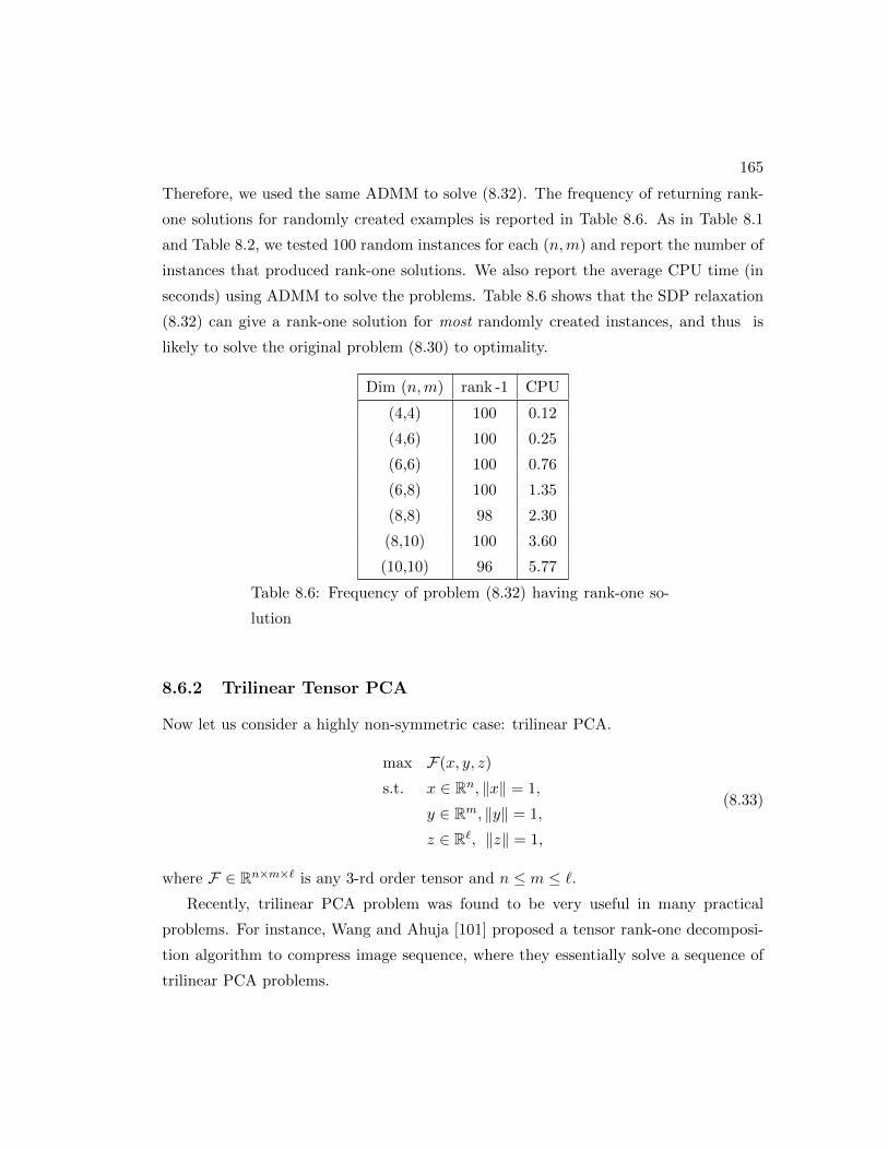
method of multipliers is proposed to solve this new formulation.

We study low-rank tensor optimization in Chapter 9. Precisely, they are low-rank

tensor completion problem and robust tensor recovery problem respectively. To make

these problems tractable, we first replace the CP-rank by the matrix-rank and then

consider their convex reformulations. Moreover, some numerical examples are provided

to show that matrix-rank works well in these problems.

Finally, in Chapter 10, we propose a cognitive approach to design phase-only modu-

lated waveforms sharing a desired ambiguity function. This problem can be formulated

as a conjugate quartic optimization with the unite circle constraint. The tensor rep-

resentation of the conjugate polynomial studied in Chapter 7 is helpful to design the

9

so-called maximum block improvement algorithm to solve this optimization problem.

The performance of this algorithm is justified by our numerical results.

1.3 Notations and Preliminaries

Throughout this thesis, we use the lower-case letters to denote vectors (e.g. x ∈ Rn),

the capital letters to denote matrices (e.g. A ∈ Rn2). For a given matrix A, we use

‖A‖∗ to denote the nuclear norm of A, which is the sum of all the singular values of A.

The boldface letter i represents the imaginary unit (i.e. i =√−1). The transpose, the

conjugate, and the conjugate transpose operators are denoted by the symbols (·)>, (·),and (·)† respectively. For any complex number z = a + ib ∈ C with a, b ∈ R, its real

part is denoted by Re z = a, and its modulus by |z| =√z†z =

√a2 + b2. For x ∈ Cn,

its norm is denoted by ‖x‖ :=(∑n

i=1 |xi|2) 1

2 .

A tensor in real field is a high dimensional array of real data, usually in calligraphic

letter, and is denoted as A = (Ai1i2···im)n1×n2×···×nm . The space where n1×n2×· · ·×nmdimensional real-valued tensor resides is denoted by Rn1×n2×···×nm . We call A super-

symmetric if n1 = n2 = · · · = nm and Ai1i2···im is invariant under any permutation

of (i1, i2, ..., im), i.e., Ai1i2···im = Aπ(i1,i2,··· ,im), π(i1, i2, · · · , im) is any permutation of

indices (i1, i2, · · · , im). The set of all distinct permutations of the indices i1, i2, · · · , idis denoted by Π(i1i2 · · · id). The space where n× n× · · · × n︸︷︷︸

m

super-symmetric tensors

reside is denoted by Snm

.

A generic form is a homogeneous polynomial function in n variables, or specifically

the function

f(x) =∑

1≤i1≤···≤im≤nai1···imxi1 · · ·xim , (1.3)

where x = (x1, · · · , xn)> ∈ Rn. In fact, super-symmetric tensors are bijectively related

to forms. In particular, restricting to m-th order tensors, for a given super-symmetric

tensorA ∈ Snm

, the form in (1.3) can be uniquely determined by the following operation:

f(x) = A(x, · · · , x︸︷︷︸m

) :=∑

1≤i1,··· ,im≤nAi1···imxi1 · · ·xim , (1.4)

where x ∈ Rn, Ai1···im = ai1···im/|Π(i1 · · · im)|, and vice versa. (This is the same as the

10

one-to-one correspondence between a symmetric matrix and a quadratic form.)

Special cases of tensors are vector (m = 1) and matrix (m = 2), and tensors can also

be seen as a long vector or a specially arranged matrix. For instance, the tensor space

Rn1×n2×···×nm can also be seen as a matrix space R(n1×n2×···×nm1 )×(nm1+1×nm1+2×···×nm),

where the row is actually an m1 array tensor space and the column is another m−m1

array tensor space. Such connections between tensor and matrix re-arrangements will

play an important role in this thesis. As a convention in this thesis, if there is no other

specification we shall adhere to the Euclidean norm (i.e. the L2-norm) for vectors and

tensors; in the latter case, the Euclidean norm is also known as the Frobenius norm,

and is sometimes denoted as ‖A‖F =√∑

i1,i2,...,imA2i1i2···im . Regarding the products,

we use ⊗ to denote the outer product for tensors; that is, for A1 ∈ Rn1×n2×···×nm and

A2 ∈ Rnm+1×nm+2×···×nm+` , A1 ⊗A2 is in Rn1×n2×···×nm+` with

(A1 ⊗A2)i1i2···im+`= (A1)i1i2···im(A2)im+1···im+`

,

and ⊗ also denotes the outer product between vectors, in other words,

(x1 ⊗ x2 ⊗ · · · ⊗ xm)i1i2···im =

m∏k=1

(xk)ik .

The inner product between tensors A1 and A2 residing in the same space Rn1×n2×···×nm

is denoted

A1 • A2 =∑

i1,i2,...,im

(A1)i1i2···im(A2)i1i2···im .

Under this light, a multi-linear form A(x1, x2, ..., xm) can also be written in inner/outer

products of tensors as

A • (x1 ⊗ · · · ⊗ xm) :=∑

i1,··· ,im

Ai1,··· ,im(x1 ⊗ · · · ⊗ xm)i1,··· ,im =∑

i1,··· ,im

Ai1,··· ,imm∏k=1

xkik .

Given an even order tensor A ∈ Sn2d

and a tensor X ∈ Rnd , we may also define the

following operation (in the same spirit as (1.4)):

A(X ,X ) :=∑

1≤i1,··· ,i2d≤nAi1···i2d Xi1···idXid+1···i2d .

Chapter 2

Cones of Nonnegative Quartic

Forms

2.1 Introduction

2.1.1 Motivation

Checking the convexity of a quadratic function boils down to testing the positive semidef-

initeness of its Hessian matrix in the domain. Since the Hessian matrix is constant, the

test can be done easily. We also mentioned the following simple-looking question due

to Shor [10] in 1992:

Given a fourth degree polynomial function in n variables, can one still easily

tell if the function is convex or not?

This question remains open for almost two decades, until recently Ahmadi et al. [11]

proved that checking the convexity of a general quartic polynomial function is actually

strongly NP-hard. This groundbreaking result helps to highlight a crucial difference

between quartic and quadratic polynomials and attracts our attention to the quartic

polynomial functions.

Among all the quartic polynomials, we are particularly interested in the nonnegative

quartic polynomials, that is the output of the polynomial function is nonnegative. This

is because there is an intrinsic connection between optimizing a polynomial function and

11

12

the description of all the polynomial functions that are nonnegative over a given domain.

For the case of quadratic polynomials and bi-quadratic function, this connection was

explored in [12] and [13] respectively. Such investigations can be traced back to the

19th century when the relationship between nonnegative polynomial functions and the

sum of squares (SOS) of polynomials was explicitly studied. Hilbert [14] in 1888 showed

that there are only three classes of nonnegative polynomial functions: (1) univariate

polynomials; (2) multivariate quadratic polynomials; (3) bivariate quartic polynomials,

which can be represented as sum of squares of polynomial functions. Since polynomial

functions with a fixed degree form a vector space, and the nonnegative polynomials and

the SOS polynomials form two convex cones respectively within that vector space, the

afore-mentioned results can be understood as a specification of three particular cases

where these two convex cones coincide, while in general of course the cone of nonnegative

polynomials is larger. There are certainly other interesting convex cones in the same

vector space. For instance, the convex polynomial functions form yet another convex

cone in that vector space. Helton and Nie [15] introduced the notion of sos-convex

polynomials, to indicate the polynomials whose Hessian matrix can be decomposed as a

sum of squares of polynomial matrices. All these classes of convex cones are important

in their own rights.

There are some substantial recent progresses along the relationships among various

nonnegative polynomials. As we mentioned earlier, e.g. the question of Shor [10] regard-

ing the complexity of deciding the convexity of a quartic polynomial was nicely settled

by Ahmadi et al. [11]. It is also natural to inquire if the Hessian matrix of a convex

polynomial is sos-convex. Ahmadi and Parrilo [43] gave an example to show that this

is not the case in general. Blekherman proved that a convex polynomial is not neces-

sary a sum of squares [44] if the degree of the polynomial is larger than two. However,

Blekherman’s proof is not constructive, and it remains an open problem of constructing

a concrete example of convex polynomial which is not a sum of squares. Reznick [45]

studied the sum of even powers of linear forms, the sum of squares of forms, and the

positive semidefinite forms.

In view of the cones formed by the polynomial functions (e.g. the cones of non-

negative polynomials, the convex polynomials, the SOS polynomials and the sos-convex

polynomials), it is natural to inquire about their relational structures, complexity status

13

and the description of their interiors. We aim to conduct a systematic study on those

topics in this chapter, to bring together much of the known results in the context of

our new findings, and to present them in a self-contained manner. In a way there is a

‘phase transition’ in terms of complexity when the scope of polynomials goes beyond

quadratics. Compared to the quadratic case (cf. Sturm and Zhang [12]), the structure of

the quartic forms is far from being clear. We believe that the class of quartic polynomial

functions (or the class of quartic forms) is an appropriate subject of study on its own

right, beyond quadratic functions (or matrices). There are at least three immediate

reasons to elaborate on the quartic polynomials, rather than polynomial functions of

other (or general) degrees. First of all, nonnegativity is naturally associated with even

degree polynomials, and the quartic polynomial is next to quadratic polynomials in that

hierarchy. Second, quartic polynomials represent a landscape after the ‘phase transi-

tion’ takes place. However, dealing with quartic polynomials is still manageable, as far

as notations are concerned. Finally, from an application point of view, quartic poly-

nomial optimization is by far the most relevant polynomial optimization model beyond

quadratic polynomials. The afore-mentioned examples such as kurtosis risks in portfolio

management ([46]), the bi-quadratic optimization models ([32]), and the nonlinear least

square formulation of sensor network localization ([47]) are all such examples. In this

chapter, due to the one-to-one correspondence between a super-symmetric tensor and

a homogenous polynomial, we provide various characterizations of several important

convex cones in the fourth order super-symmetric tensor space, present their relational

structures and work out their complexity status. Therefore, our results can be helpful

in tensor optimization (see [48, 49] for recent development in sparse or low rank tensor

optimization). We shall also motivate the study by some examples from applications.

2.1.2 Introducing the Quartic Forms

In this subsection we shall formally introduce the definitions of the quartic forms in the

super-symmetric fourth order tensor space. The set of n-dimensional super-symmetric

fourth order tensors is denoted by Sn4. In the remainder of this chapter, we shall

frequently use a super-symmetric tensor F ∈ Sn4

to indicate a quartic form F(x, x, x, x),

i.e., the notion of “super-symmetric fourth order tensor” and “quartic form” are used

interchangeably.

14

Let us start with the well known notion of positive semidefinite (PSD) and the sum

of squares (SOS) of polynomials.

Definition 2.1.1. A quartic form F ∈ Sn4

is called quartic PSD if

F(x, x, x, x) ≥ 0 ∀x ∈ Rn. (2.1)

The set of all quartic PSD forms in Sn4

is denoted by Sn4

+ .

If a quartic form F ∈ Sn4

can be written as a sum of squares of polynomial functions,

then these polynomials must be quadratic forms, i.e.,

F(x, x, x, x) =m∑i=1

(x>Aix

)2= (x⊗ x⊗ x⊗ x) •

m∑i=1

Ai ⊗Ai,

where Ai ∈ Sn2, the set of symmetric matrices. However,

∑mi=1

(Ai ⊗Ai

)∈−→S n4

is

only partial-symmetric, and may not be exactly F , which must be super-symmetric. To

place it in the family Sn4, a symmetrization operation is required. Since x⊗ x⊗ x⊗ x

is super-symmetric, we still have (x⊗ x⊗ x⊗ x) • sym(∑m

i=1Ai ⊗Ai

)= (x⊗ x⊗ x⊗

x) •∑m

i=1Ai ⊗Ai.


is called quartic SOS if F(x, x, x, x) is a sum

of squares of quadratic forms, i.e., there exist m symmetric matrices A1, . . . , Am ∈ Sn2

such that

F = sym

(m∑i=1

Ai ⊗Ai)

=m∑i=1

sym(Ai ⊗Ai

).

The set of quartic SOS forms in Sn4

is denoted by Σ2n,4.

As all quartic SOS forms constitute a convex cone, we have

Σ2n,4 = sym cone

A⊗A |A ∈ Sn

2.

Usually, for a given F = sym(∑m

i=1Ai ⊗Ai

)it maybe a challenge to write it explicitly

as a sum of squares, although the construction can in principle be done in polynomial-

time by semidefinte programming (SDP), which however is costly. In this sense, having

a quartic SOS tensor in super-symmetric form may not always be beneficial, since the

super-symmetry can destroy the SOS structure.

Since F(X,X) is a quadratic form, the usual sense of nonnegativity carries over.

Formally we introduce this notion below.

15


is called quartic matrix PSD if

F(X,X) ≥ 0 ∀X ∈ Rn2.

The set of quartic matrix PSD forms in Sn4

is denoted by Sn2×n2

+ .

We remark that the matrix PSD forms is essentially equivalent to the cone of PSD

moment matrices; see e.g. [50]. But our definition here is more clear and straightforward.

Related to the sum of squares for quartic forms, we now introduce the notion to the

sum of quartics (SOQ): If a quartic form F ∈ Sn4

is SOQ, then there are m vectors

a1, . . . , am ∈ Rn such that

F(x, x, x, x) =m∑i=1

(x>ai

)4= (x⊗ x⊗ x⊗ x) •

m∑i=1

ai ⊗ ai ⊗ ai ⊗ ai.


is called quartic SOQ if F(x, x, x, x) is a

sum of fourth powers of linear forms, i.e., there exist m vectors a1, . . . , am ∈ Rn such

that

F =m∑i=1

ai ⊗ ai ⊗ ai ⊗ ai.

The set of quartic SOQ forms in Sn4

is denoted by Σ4n,4.

As all quartic SOQ forms also constitute a convex cone, we denote

Σ4n,4 = cone a⊗ a⊗ a⊗ a | a ∈ Rn ⊆ Σ2

n,4.

In the case of quadratic functions, it is well known that for a given homogeneous

form (i.e., a symmetric matrix, for that matter) A ∈ Sn2

the following two statements

are equivalent:

• A is positive semidefinite (PSD): A(x, x) := x>Ax ≥ 0 for all x ∈ Rn.

• A is a sum of squares (SOS): A(x, x) =∑m

i=1(x>ai)2 (or equivalently A =∑mi=1 a

i ⊗ ai) for some a1, . . . , am ∈ Rn.

It is therefore clear that the four types of quartic forms defined above are actually

different extensions of the nonnegativity. In particular, quartic PSD and quartic matrix

PSD forms are extended from quadratic PSD, while quartic SOS and SOQ forms are in

16

the form of summation of nonnegative polynomials, and are extended from quadratic

SOS. We will show later that there is an interesting hierarchical relationship for general

n:

Σ4n,4 ( Sn

2×n2

+ ( Σ2n,4 ( Sn

4

+ . (2.2)

Recently, a class of polynomials termed the sos-convex polynomials (cf. Helton and

Nie [15]) has been brought to attention, which is defined as follows (see [51] for three

other equivalent definitions of the sos-convexity):

A multivariate polynomial function f(x) is sos-convex if its Hessian matrix

H(x) can be factorized as H(x) = (M(x))>M(x) with a polynomial matrix

M(x).

The reader is referred to [43] for applications of the sos-convex polynomials. In this

chapter, we shall focus on Sn4

and investigate sos-convex quartic forms with the hier-

archy (2.2). For a quartic form F ∈ Sn4, it is straightforward to compute its Hessian

matrix H(x) = 12F(x, x, ·, ·), i.e.,

(H(x))ij = 12F(x, x, ei, ej) ∀ 1 ≤ i, j ≤ n,

where ei ∈ Rn is the vector whose i-th entry is 1 and other entries are zeros. Therefore

H(x) is a quadratic matrix of x. If H(x) can be decomposed as H(x) = (M(x))>M(x)

with M(x) being a polynomial matrix, then M(x) must be linear with respect to x.


is called quartic sos-convex, if there exists

a linear matrix M(x) of x, such that its Hessian matrix

12F(x, x, ·, ·) = (M(x))>M(x).

The set of quartic sos-convex forms in Sn4

is denoted by Σ2∇2n,4

.

Helton and Nie [15] proved that a nonnegative polynomial is sos-convex, then it must

be SOS. In particular, if the polynomial is a quartic form, by denoting the i-th row of the

linear matrix M(x) to be x>Ai for i = 1, . . . ,m and some matrices A1, . . . , Am ∈ Rn2,

then (M(x))>M(x) =∑m

i=1(Ai)>xx>Ai. Therefore

F(x, x, x, x) = x>F(x, x, ·, ·)x =1

12x>(M(x))>M(x)x =

1

12

m∑i=1

(x>Aix

)2∈ Σ2

n,4.

17

In addition, the Hessian matrix for a quartic sos-convex form is obviously positive

semidefinite for any x ∈ Rn. Hence sos-convexity implies convexity. Combining these

two facts, we conclude that a quartic sos-convex form is both SOS and convex, which

motivates us to study the last quartic forms in this chapter.


is called convex and SOS, if it is both

quartic SOS and convex. The set of quartic convex and SOS forms in Sn4

is denoted by

Σ2n,4

⋂Sn

4

cvx.

Here Sn4

cvx is denoted to be the set of all convex quartic forms in Sn4.

2.1.3 The Contributions and the Organization

All the sets of the quartic forms defined in Section 2.1.2 are clearly convex cones. The

remainder of this chapter is organized as follows. In Section 2.2, we start by studying

the cones: Sn4

+ , Σ2n,4, Sn

2×n2

+ , and Σ4n,4. We first show that they are all closed, and that

they can be presented in different formulations. As an example, the cone of quartic

SOQ forms is

Σ4n,4 = cone a⊗ a⊗ a⊗ a | a ∈ Rn = sym cone

A⊗A |A ∈ Sn

2

+ , rank (A) = 1,

which can also be written as

sym coneA⊗A |A ∈ Sn

2

+

,

meaning that the rank-one constraint can be removed without affecting the cone itself.

We know that among these four cones there are two primal-dual pairs: Sn4

+ is dual

to Σ4n,4, and Σ2

n,4 is dual to Sn2×n2

+ , and a hierarchical relationship Σ4n,4 ( Sn

2×n2

+ (Σ2n,4 ( Sn

4

+ exists. Although all these results can be found in [45, 50] thanks to various

representations of quartic forms, it is beneficial to present them in a unified manner

in the super-symmetric tensor space. Moreover, the tensor representation of quartic

forms has interest in its own right. For instance, it sheds some light on how symmetric

property changes the nature of quartic cones. To see this, let us consider an SOS

quartic form∑m

i=1(x>Aix)2, which will become quartic matrix PSD if∑m

i=1Ai ⊗Ai is

already a super-symmetric tensor (Theorem 2.2.3). If we further assume m = 1, then

we have rank (A1) = 1 (Theorem 2.4 in [52]) meaning that A1 ⊗A1 = a⊗ a⊗ a⊗ a for

18

some a, is quartic SOQ. Besides, explicit examples are also very important for people

to understand the quartic functions. It is worth mentioning that the main work of

Ahmadi and Parrilo [43] is to provide a polynomial which is convex but not sos-convex.

Here we present a new explicit quartic form, which is matrix PSD but not SOQ; see

Example 2.2.11.

In Section 2.3, we further study two more cones: Σ2∇2n,4

and Σ2n,4

⋂Sn

4

cvx. Inter-

estingly, these two new cones can be nicely placed in the hierarchical scheme (2.2) for

general n:

Σ4n,4 ( Sn

2×n2

+ ( Σ2∇2n,4⊆(Σ2n,4

⋂Sn

4

cvx

)( Σ2

n,4 ( Sn4

+ . (2.3)

The complexity status of all these cones are summarized in Section 2.4, including

some well known results in the literature, our new finding is that testing the convexity

is still NP-hard even for sums of squares quartic forms (Theorem 2.4.4). As a result,

we show that Σ2∇2n,4((Σ2n,4

⋂Sn

4

cvx

)unless P = NP , completing the picture presented

in (2.3), on the premise that P 6= NP . The low dimensional cases of these cones are

also discussed in Section 2.4. Specially, for the case n = 2, all the six cones reduce

to only two distinctive ones, and for the case n = 3, they reduce to exactly three

distinctive cones. In addition, we study two particular simple quartic forms:(x>x

)2and∑n

i=1 xi4. Since they both belong to Σ4

n,4, which is the smallest cone in our hierarchy,

one may ask whether or not they belong to the interior of Σ4n,4. Intuitively, it may

appear plausible that∑n

i=1 xi4 is in the interior of Σ4

n,4, for it is the quartic extension

of quadratic unite form∑n

i=1 xi2. However, our results show that

∑ni=1 xi

4 is not in

Int (Sn4

cvx) ) Int (Σ4n,4) but in Int (Σ2

n,4) (Theorem 2.4.10), and(x>x

)2is actually in

Int (Σ4n,4) (Theorem 2.4.11), implying that

(x>x

)2is more ‘positive’ than

∑ni=1 xi

4.

Finally, in Section 2.5 we discuss applications of quartic conic programming, includ-

ing bi-quadratic assignment problems and eigenvalues of super-symmetric tensors.

2.2 Quartic PSD Forms, Quartic SOS Forms, and the Dual

Cones

Let us now consider the first four cones of quartic forms introduced in Section 2.1.2:

Σ4n,4, Sn

2×n2

+ , Σ2n,4, and Sn

4

+ .

19

2.2.1 Closedness

Proposition 2.2.1. Σ4n,4, Sn

2×n2

+ , Σ2n,4, and Sn

4

+ are all closed convex cones.

While Sn4

+ and Sn2×n2

+ are evidently closed, by a similar argument as in [12] it is also

easy to see that the cone of quartic SOS forms Σ2n,4 := sym cone

A⊗A |A ∈ Sn

2

is closed. The closedness of Sn2×n2

+ , Σ2n,4 and Sn

4

+ were also known in polynomial

optimization, e.g. [50]. The closedness of the cone of quartic SOQ forms Σ4n,4 was

proved in Proposition 3.6 of [45] for general even degree forms. In fact, we have a

slightly stronger result below:

Lemma 2.2.2. If D ⊆ Rn is closed, then cone a⊗ a⊗ a⊗ a | a ∈ D is closed.

Proof. Suppose that F ∈ cl cone a⊗ a⊗ a⊗ a | a ∈ D, then there is a sequence

of quartic forms Fk ∈ cone a⊗ a⊗ a⊗ a | a ∈ D (k = 1, 2, . . . ), such that F =

limk→∞Fk. Since the dimension of Sn4

is N :=(n+3

4

), it follows from Caratheodory’s

theorem that for any given Fk, there exists an n× (N + 1) matrix Zk, such that

Fk =N+1∑i=1

zk(i)⊗ zk(i)⊗ zk(i)⊗ zk(i),

where zk(i) is the i-th column vector of Zk, and is a positive multiple of a vector in D.

Now define trFk =∑n

j=1Fkjjjj , then

N+1∑i=1

n∑j=1

(Zkji)4 = trFk → trF .

Thus, the sequence Zk is bounded, and have a cluster point Z∗, satisfying F =∑N+1i=1 z∗(i) ⊗ z∗(i) ⊗ z∗(i) ⊗ z∗(i). Note that each column of Z∗ is also a positive

multiple of a vector in D, it follows that F ∈ cone a⊗ a⊗ a⊗ a | a ∈ D.

The cone of quartic SOQ forms is closely related to the fourth moment of a multi-

dimensional random variable. Given an n-dimensional random variable ξ = (ξ1, . . . , ξn)>

on the support set D ⊆ Rn with density function p, its fourth moment is a super-

symmetric fourth order tensor M∈ Sn4, whose (i, j, k, `)-th entry is

Mijk` = E [ξiξjξkξ`] =

∫Dxixjxkx` p(x)dx.

20

Suppose the fourth moment of ξ is finite, then by the closedness of Σ4n,4, we have

M = E [ξ ⊗ ξ ⊗ ξ ⊗ ξ] =

∫D

(x⊗x⊗x⊗x) p(x)dx ∈ cone a⊗ a⊗ a⊗ a | a ∈ Rn = Σ4n,4.

Conversely, for any M ∈ Σ4n,4, it is easy to verify that there exists an n-dimensional

random variable whose fourth moment is just M. Thus, the set of all the finite fourth

moments of n-dimensional random variables is exactly Σ4n,4, similar to the fact that all

possible covariance matrices form the cone of positive semidefinite matrices.

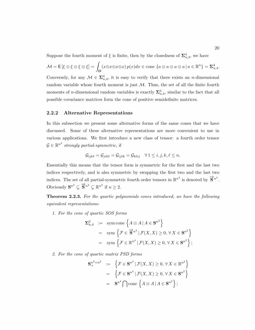
2.2.2 Alternative Representations

In this subsection we present some alternative forms of the same cones that we have

discussed. Some of these alternative representations are more convenient to use in

various applications. We first introduce a new class of tensor: a fourth order tensor

G ∈ Rn4strongly partial-symmetric, if

Gijk` = Gjik` = Gij`k = Gkìj ∀ 1 ≤ i, j, k, ` ≤ n.

Essentially this means that the tensor form is symmetric for the first and the last two

indices respectively, and is also symmetric by swapping the first two and the last two

indices. The set of all partial-symmetric fourth order tensors in Rn4is denoted by

−→S n4

.

Obviously Sn4 (−→S n4 ( Rn4

if n ≥ 2.

Theorem 2.2.3. For the quartic polynomials cones introduced, we have the following

equivalent representations:

1. For the cone of quartic SOS forms

Σ2n,4 := sym cone

A⊗A |A ∈ Sn

2

= symF ∈

−→S n4 | F(X,X) ≥ 0, ∀X ∈ Sn

2

= symF ∈ Rn4 | F(X,X) ≥ 0, ∀X ∈ Sn

2

;

2. For the cone of quartic matrix PSD forms

Sn2×n2

+ :=F ∈ Sn

4 | F(X,X) ≥ 0, ∀X ∈ Rn2

=F ∈ Sn

4 | F(X,X) ≥ 0, ∀X ∈ Sn2

= Sn4⋂

coneA⊗A |A ∈ Sn

2

;

21

3. For the cone of quartic SOQ forms

Σ4n,4 := cone a⊗ a⊗ a⊗ a | a ∈ Rn = sym cone

A⊗A |A ∈ Sn

2

+

.

The remaining of this subsection is devoted to the proof of Theorem 2.2.3.

Let us first study the equivalent representations for Σ2n,4 and Sn

2×n2

+ . To verify a

quartic matrix PSD form, we should check the operations of quartic forms on matrices.

In fact, the quartic matrix PSD forms can be extended to the space of strongly partial-

symmetric tensors−→S n4

. It is not hard to verify that for any F ∈−→S n4

, it holds that

F(X,Y ) = F(X>, Y ) = F(X,Y >) = F(Y,X) ∀X,Y ∈ Rn2, (2.4)

which implies that F(X,Y ) is invariant under the transpose operation as well as the

operation to swap the X and Y matrices. Indeed, it is easy to see that the partial-

symmetry of F is a necessary and sufficient condition for (2.4) to hold. We have the

following property for quartic matrix PSD forms in−→S n4

, similar to that for Sn2×n2

+ in

Theorem 2.2.3.

Lemma 2.2.4. For strongly partial-symmetric four order tensors, it holds that

−→S n2×n2

+ :=F ∈

−→S n4 | F(X,X) ≥ 0, ∀X ∈ Rn2

=

F ∈

−→S n4 | F(X,X) ≥ 0, ∀X ∈ Sn

2

(2.5)

= coneA⊗A |A ∈ Sn

2. (2.6)

Proof. Observe that for any skew-symmetric Y ∈ Rn2, i.e., Y > = −Y , we have

F(X,Y ) = −F(X,−Y ) = −F(X,Y >) = −F(X,Y ) ∀X ∈ Rn2,

which implies that F(X,Y ) = 0. As any square matrix can be written as the sum

of a symmetric matrix and a skew-symmetric matrix, say for Z ∈ Rn2, by letting

X = (Z + Z>)/2 which is symmetric, and Y = (Z − Z>)/2 which is skew-symmetric,

we have Z = X + Y . Therefore,

F(Z,Z) = F(X + Y,X + Y ) = F(X,X) + 2F(X,Y ) + F(Y, Y ) = F(X,X).

This implies the equivalence between F(X,X) ≥ 0, ∀X ∈ Rn2and F(X,X) ≥ 0, ∀X ∈

Sn2, which proves (2.5).

22

To prove (2.6), first note that coneA⊗A |A ∈ Sn

2⊆ F ∈

−→S n4 | F(X,X) ≥

0, ∀X ∈ Rn2. Conversely, given any G ∈−→S n4

with G(X,X) ≥ 0, ∀X ∈ Rn2, we may

rewrite G as an n2 × n2 symmetric matrix MG . Therefore

(vec (X))>MG vec (X) = G(X,X) ≥ 0 ∀X ∈ Rn2,

which implies that MG is positive semidefinite. Let MG =∑m

i=1 zi(zi)>, where

zi =(zi11, . . . , z

i1n, . . . , z

in1, . . . , z

inn

)> ∀ 1 ≤ i ≤ m.

Note that for any 1 ≤ k, ` ≤ n, Gk``k =∑m

i=1 zik`z

i`k, Gk`k` =

∑mi=1(zik`)

2 and G`k`k =∑mi=1(zi`k)

2, as well as Gk``k = Gk`k` = G`k`k by partial-symmetry of G. We have

m∑i=1

(zik` − zi`k)2 =

m∑i=1

(zik`)2 +

m∑i=1

(zi`k)2 − 2

m∑i=1

zik`zi`k = Gk`k` + G`k`k − 2Gk``k = 0,

which implies that zik` = zi`k for any 1 ≤ k, ` ≤ n. Therefore, we may construct a

symmetric matrix Zi ∈ Sn2, such that vec (Zi) = zi for all 1 ≤ i ≤ m. We have

G =∑m

i=1 Zi ⊗ Zi, and so (2.6) is proven.

For the first part of Theorem 2.2.3, the first identity follows from (2.6) by apply-

ing the symmetrization operation on both sides. The second identity is quite obvious.

Essentially, for any F ∈ Rn4, we may make it being strongly partial-symmetric by

averaging the corresponding entries, to be denoted by F0 ∈−→S n4

. It is easy to see

that F0(X,X) = F(X,X) for all X ∈ Sn2

since X ⊗ X ∈−→S n4

, which implies thatF ∈ Rn4 | F(X,X) ≥ 0, ∀X ∈ Sn

2⊆F ∈

−→S n4 | F(X,X) ≥ 0, ∀X ∈ Sn

2

. The re-

verse inclusion is trivial.

For the second part of Theorem 2.2.3, it follows from (2.5) and (2.6) by restricting to

Sn4. Let us now turn to proving the last part of Theorem 2.2.3, which is an alternative

representation of the quartic SOQ forms. Obviously we need only to show that

sym coneA⊗A |A ∈ Sn

2

+

⊆ cone a⊗ a⊗ a⊗ a | a ∈ Rn .

Since there is a one-to-one mapping from quartic forms to fourth order super-symmetric

tensors, it suffices to show that for any A ∈ Sn2

+ , the function (x>Ax)2 can be written

as a form of∑m

i=1(x>ai)4 for some a1, . . . , am ∈ Rn. Note that the so-called Hilbert’s

identity (see e.g. Barvinok [18]) asserts the following:

23

For any fixed positive integers d and n, there always exist m real vectors

a1, . . . , am ∈ Rn such that (x>x)d =∑m

i=1(x>ai)2d.

In fact, when d = 2, we shall propose a polynomial-time algorithm to find the afore-

mentioned representations, in Chapter 3, where the number m is bounded by a polyno-

mial of n, although in the original version of Hilbert’s identity m is exponential in n.

Since we have A ∈ Sn2

+ , replacing x by A1/2y in Hilbert’s identity when d = 2, one gets

(y>Ay)2 =∑m

i=1(y>A1/2ai)4. The desired decomposition follows, and this proves the

last part of Theorem 2.2.3.

2.2.3 Duality

In this subsection, we shall discuss the duality relationships among these four cones of

quartic forms. Note that Sn4

is the ground vector space within which the duality is

defined, unless otherwise specified.

Theorem 2.2.5. The cone of quartic PSD forms and the cone of quartic SOQ forms

are primal-dual pair, i.e., Σ4n,4 =

(Sn

4

+

)∗and Sn

4

+ =(Σ4n,4

)∗. The cone of quartic SOS

forms and the cone of quartic matrix PSD forms are primal-dual pair, i.e., Sn2×n2

+ =(Σ2n,4

)∗and Σ2

n,4 =(Sn

2×n2

+

)∗.

Remark that the primal-dual relationship between Σ4n,4 and Sn

4

+ was already proved

in Theorem 3.7 of [45] for general even degree forms. The primal-dual relationship

between Sn2×n2

+ and Σ2n,4 was also mentioned in Theorem 3.16 of [45] for general even

degree forms. Here we give the proof in the language of quartic tensors. Let us start by

discussing the primal-dual pair Σ4n,4 and Sn

4

+ . In Proposition 1 of [12], Sturm and Zhang

proved that for the quadratic forms, A ∈ Sn2 |x>Ax ≥ 0, ∀x ∈ D and cone aa> | a ∈

D are a primal-dual pair for any closed D ⊆ Rn. We observe that a similar structure

holds for the quartic forms as well. The first part of Theorem 2.2.5 then follows from

next lemma.

Lemma 2.2.6. If D ⊆ Rn is closed, then Sn4

+ (D) := F ∈ Sn4 | F(x, x, x, x) ≥ 0, ∀x ∈

D and cone a⊗ a⊗ a⊗ a | a ∈ D are a primal-dual pair, i.e.,

Sn4

+ (D) = (cone a⊗ a⊗ a⊗ a | a ∈ D)∗ (2.7)

24

and (Sn

4

+ (D))∗

= cone a⊗ a⊗ a⊗ a | a ∈ D.

Proof. Since cone a ⊗ a ⊗ a ⊗ a | a ∈ D is closed by Lemma 2.2.2, we only need to

show (2.7). In fact, if F ∈ Sn4

+ (D), then F • (a ⊗ a ⊗ a ⊗ a) = F(a, a, a, a) ≥ 0 for all

a ∈ D. Thus F • G ≥ 0 for all G ∈ cone a ⊗ a ⊗ a ⊗ a | a ∈ D, which implies that

F ∈ (cone a⊗ a⊗ a⊗ a | a ∈ D)∗. Conversely, if F ∈ (cone a⊗ a⊗ a⊗ a | a ∈ D)∗,then F • G ≥ 0 for all G ∈ cone a ⊗ a ⊗ a ⊗ a | a ∈ D. In particular, by letting

G = x⊗ x⊗ x⊗ x, we have F(x, x, x, x) = F • (x⊗ x⊗ x⊗ x) ≥ 0 for all x ∈ D, which

implies that F ∈ Sn4

+ (D).

Let us turn to the primal-dual pair of Sn2×n2

+ and Σ2n,4. For technical reasons,

we shall momentarily lift the ground space from Sn4

to the space of strongly partial-

symmetric tensors−→S n4

. This enlarges all the dual objects. To distinguish these two dual

objects, let us use the notation ‘K−→∗ ’ to indicate the dual of convex cone K ∈ Sn

4 ⊆−→S n4

generated in the space−→S n4

, while ‘K∗’ is the dual of K generated in the space Sn4.

Lemma 2.2.7. For strongly partial-symmetric tensors, the cone−→S n2×n2

+ is self-dual

with respect to the space−→S n4

, i.e.,−→S n2×n2

+ =(−→

S n2×n2

+

)−→∗.

Proof. According to Proposition 1 of [12] and the partial-symmetry of−→S n4

, we have(cone

A⊗A |A ∈ Sn

2)−→∗

=F ∈

−→S n4 | F(X,X) ≥ 0, ∀X ∈ Sn

2.

By Lemma 2.2.4, we have

−→S n2×n2

+ =F ∈

−→S n4 | F(X,X) ≥ 0, ∀X ∈ Sn

2

= coneA⊗A |A ∈ Sn

2.

Thus−→S n2×n2

+ is self-dual with respect to the space−→S n4

.

Notice that by definition and Lemma 2.2.7, we have

Σ2n,4 = sym cone

A⊗A |A ∈ Sn

2

= sym−→S n2×n2

+ = sym(−→

S n2×n2

+

)−→∗,

and by the alternative representation in Theorem 2.2.3 we have

Sn2×n2

+ = Sn4⋂

coneA⊗A |A ∈ Sn

2

= Sn4⋂−→

S n2×n2

+ .

25

Therefore the duality between Sn2×n2

+ and Σ2n,4 follows immediately from the following

lemma.

Lemma 2.2.8. If K ⊆−→S n4

is a closed convex cone and K−→∗ is its dual with respect

to the space−→S n4

, then K⋂

Sn4

and sym K−→∗ are a primal-dual pair with respect to the

space Sn4, i.e.,

(K⋂

Sn4)∗

= sym K−→∗ and K

⋂Sn

4=(

sym K−→∗)∗

.

Proof. For any G ∈ sym K−→∗ ⊆ Sn

4, there is a G′ ∈ K

−→∗ ⊆−→S n4

, such that G = symG′ ∈Sn

4. We then have Gijk` = 1

3(G′ijk` + G′ikj` + G′i`jk). Thus for any F ∈ K⋂

Sn4 ⊆ Sn

4, it

follows that

F • G =∑

1≤i,j,k,`≤n

Fijk`(G′ijk` + G′ikj` + G′i`jk)3

=∑

1≤i,j,k,`≤n

Fijk`G′ijk` + Fikj`G′ikj` + Fi`jkG′i`jk3

= F • G′ ≥ 0.

Therefore G ∈(K⋂

Sn4)∗

, implying that sym K−→∗ ⊆

(K⋂

Sn4)∗

.

Moreover, if F ∈(

sym K−→∗)∗⊆ Sn

4, then for any G′ ∈ K

−→∗ ⊆−→S n4

, we have

G = symG′ ∈ sym K−→∗ , and G′ • F = G • F ≥ 0. Therefore F ∈

(K−→∗)−→∗

= cl K = K,

which implies that(

sym K−→∗)∗⊆(K⋂

Sn4)

. Finally, the duality relationship holds

by the bipolar theorem and the closedness of these cones.

2.2.4 The Hierarchical Structure

The last part of this section is to present a hierarchy among these four cones of quartic

forms. The main result is summarized in the theorem below.

Theorem 2.2.9. If n ≥ 4, then

Σ4n,4 ( Sn

2×n2

+ ( Σ2n,4 ( Sn

4

+ .

For the low dimension cases (n ≤ 3), we shall present it in Section 2.4.2. Evidently

a quartic SOS form is quartic PSD, implying Σ2n,4 ⊆ Sn

4

+ . By invoking the duality

operation and using Theorem 2.2.5 we have Σ4n,4 ⊆ Sn

2×n2

+ , while by the alternative

26

representation in Theorem 2.2.3 we have Sn2×n2

+ = Sn4 ⋂

coneA⊗A |A ∈ Sn

2

, and

by the very definition we have Σ2n,4 = sym cone

A⊗A |A ∈ Sn

2

. Therefore Sn2×n2

+ ⊆Σ2n,4. Finally, the strict containing relationship is a result of the following examples.

Example 2.2.10. (Quartic forms in Sn4

+ \ Σ2n,4 when n = 4). Let g1(x) = x1

2(x1 −x4)2 +x2

2(x2−x4)2 +x32(x3−x4)2 +2x1x2x3(x1 +x2 +x3−2x4) and g2(x) = x1

2x22 +

x22x3

2 +x32x1

2 +x44−4x1x2x3x4, then both g1(x) and g2(x) are in S44

+ \Σ24,4. We refer

the interested readers to [53] for more information on these examples and the study on

these two cones.

Example 2.2.11. (A quartic form in Sn2×n2

+ \Σ4n,4 when n = 4). Construct F ∈ S44

,

whose only nonzero entries (taking into account the super-symmetry) are F1122 = 4,

F1133 = 4, F2233 = 4, F1144 = 9, F2244 = 9, F3344 = 9, F1234 = 6, F1111 = 29,

F2222 = 29, F3333 = 29, and F4444 = 3 + 257 . One may verify straightforwardly that F

can be decomposed as∑7

i=1Ai ⊗Ai, with A1 =

√

7 0 0 0

0√

7 0 0

0 0√

7 0

0 0 0 5√7

,

A2 =

0 2 0 0

2 0 0 0

0 0 0 3

0 0 3 0

, A3 =

0 0 2 0

0 0 0 3

2 0 0 0

0 3 0 0

, A4 =

0 0 0 3

0 0 2 0

0 2 0 0

3 0 0 0

,

A5 =

−2 0 0 0

0 3 0 0

0 0 3 0

0 0 0 1

, A6 =

3 0 0 0

0 −2 0 0

0 0 3 0

0 0 0 1

, and A7 =

3 0 0 0

0 3 0 0

0 0 −2 0

0 0 0 1

.

According to Theorem 2.2.3, we have F ∈ S42×42

+ . Recall g2(x) in Example 2.2.10, which

is quartic PSD. Denote G to be the super-symmetric tensor associated with g2(x), thus

G ∈ S44

+ . One computes that G • F = 4 + 4 + 4 + 3 + 257 − 24 < 0. By the duality result

as stipulated in Theorem 2.2.5, we conclude that F /∈ Σ44,4.

Example 2.2.12. (A quartic form in Σ2n,4 \ Sn

2×n2

+ when n = 3). Let g3(x) = 2x14 +

2x24 + 1

2x34 +6x1

2x32 +6x2

2x32 +6x1

2x22, which is obviously quartic SOS. Now recycle

27

the notation and denote G ∈ Σ23,4 to be the super-symmetric tensor associated with g3(x),

and we have G1111 = 2, G2222 = 2, G3333 = 12 , G1122 = 1, G1133 = 1, and G2233 = 1. If

we let X = Diag (1, 1,−4) ∈ S32, then

G(X,X) =∑

1≤i,j,k,`≤3

Gijk`XijXk` =∑

1≤i,k≤3

GiikkXiiXkk =

1

1

−4

>

2 1 1

1 2 1

1 1 12

1

1

−4

= −2,

implying that G /∈ S32×32

+ .

2.3 Cones Related to Convex Quartic Forms

In this section we shall study the cone of quartic sos-convex forms Σ2∇2n,4

, and the cone

of quartic forms which are both SOS and convex Σ2n,4

⋂Sn

4

cvx. The aim is to incorporate

these two new cones into the hierarchical structure as depicted in Theorem 2.2.9.

Theorem 2.3.1. If n ≥ 4, then

Σ4n,4 ( Sn

2×n2

+ ( Σ2∇2n,4⊆(Σ2n,4

⋂Sn

4

cvx

)( Σ2

n,4 ( Sn4

+ .

As mentioned in Section 2.1.2, an sos-convex homogeneous quartic polynomial func-

tion is both SOS and convex (see also [43]), which implies that Σ2∇2n,4⊆(Σ2n,4

⋂Sn

4

cvx

).

Moreover, the following example shows that a quartic SOS form is not necessarily con-

vex.

Example 2.3.2. (A quartic form in Σ2n,4\Sn

4

cvx when n = 2). Let g4(x) = (x>Ax)2 with

A ∈ Sn2, and its Hessian matrix is ∇2g4(x) = 8Axx>A + 4x>AxA. In particular, by

letting A =

[−3 0

0 1

]and x =

(0

1

), we have ∇2f(x) =

[0 0

0 8

]+

[−12 0

0 4

] 0,

implying that g4(x) is not convex.

The above example suggests that(Σ2n,4

⋂Sn

4

cvx

)( Σ2

n,4 when n ≥ 2. Next we shall

prove the assertion that Sn2×n2

+ ( Σ2∇2n,4

when n ≥ 3. To this end, let us first quote a

result on the sos-convex functions due to Ahmadi and Parrilo [43]:

28

If f(x) is a polynomial with its Hessian matrix being ∇2f(x), then f(x) is

sos-convex if and only if y>∇2f(x)y is a sum of squares in (x, y).

For a quartic form F(x, x, x, x), its Hessian matrix is 12F(x, x, ·, ·). Therefore, Fis quartic sos-convex if and only if F(x, x, y, y) is is a sum of squares in (x, y). Now if

F ∈ Sn2×n2

+ , then by Theorem 2.2.3 we may find matrices A1, . . . , Am ∈ Sn2

such that

F =∑m

t=1At ⊗At. We have

F(x, x, y, y) = F(x, y, x, y) =

m∑t=1

∑1≤i,j,k,`≤n

xiyjxkyÀtijA

tk`

=m∑t=1

∑1≤i,j≤n

xiyjAtij

∑1≤k,`≤n

xkyÀtk`

=m∑t=1

(x>Aty

)2,

which is a sum of squares in (x, y), hence sos-convex. This proves Sn2×n2

+ ⊆ Σ2∇2n,4

, and

the example below rules out the equality when n ≥ 3.

Example 2.3.3. (A quartic form in Σ2∇2n,4\ Sn

2×n2

+ when n = 3). Recall g3(x) =

2x14 + 2x2

4 + 12x3

4 + 6x12x3

2 + 6x22x3

2 + 6x12x2

2 in Example 2.2.12, which is shown

not to be quartic matrix PSD. Moreover, it is straightforward to compute that

∇2g3(x) = 24

x1

x2

x32

x1

x2

x32

>

+ 12

0

x3

x2

0

x3

x2

>

+ 12

x3

0

x1

x3

0

x1

>

+ 12

x2

2 0 0

0 x12 0

0 0 0

0,

which implies that g3(x) is quartic sos-convex.

A natural question regarding to the hierarchical structure in Theorem 2.3.1 is whether

Σ2n,4

⋂Sn

4

cvx = Σ2∇2n,4

or not. In fact, the relationship between convex, sos-convex, and

SOS is a highly interesting subject which attracted many speculations in the literature.

Ahmadi and Parrilo [43] gave an explicit example with a three dimensional homoge-

neous form of degree eight, which they showed to be both convex and SOS but not

sos-convex. However, for quartic polynomials (degree four), such an explicit instant in

29(Σ2n,4

⋂Sn

4

cvx

)\ Σ2

∇2n,4

is not in sight. Notwithstanding the difficulty in constructing

an explicit quartic example, on the premise that P 6= NP in Section 2.4 we will show

that(Σ2n,4

⋂Sn

4

cvx

)6= Σ2

∇2n,4

. With that piece of information, the chain of containing

relations manifested in Theorem 2.3.1 is complete, under the assumption that P 6= NP .

However, the following open question remains:

Question 2.3.1. Find an explicit instant in(Σ2n,4

⋂Sn

4

cvx

)\Σ2∇2n,4

: a quartic form that

is both SOS and convex, but not sos-convex.

The two newly introduced cones in this section are related to the convexity prop-

erties. Some more words on convex quartic forms are in order here. As mentioned in

Section 2.1.2, for a quartic form F ∈ Sn4

cvx, its Hessian matrix is 12F(x, x, ·, ·). There-

fore, F is convex if and only if F(x, x, ·, ·) 0 for all x ∈ Rn, which is equivalent to

F(x, x, y, y) ≥ 0 for all x, y ∈ Rn. In fact, it is also equivalent to F(X,Y ) ≥ 0 for all

X,Y ∈ Sn2

+ . To see why, we first decompose the positive semidefinite matrices X and

Y , and let X =∑n

i=1 xi(xi)> and Y =

∑nj=1 y

j(yj)> (see e.g. Sturm and Zhang [12]).

Then

F(X,Y ) = F

n∑i=1

xi(xi)>,n∑j=1

yj(yj)>

=

∑1≤i,j≤n

F(xi(xi)>, yj(yj)>

)=

∑1≤i,j≤n

F(xi, xi, yj , yj

)≥ 0,

if F(x, x, y, y) ≥ 0 for all x, y ∈ Rn. Note that the converse is trivial, as it reduces to

let X and Y be rank-one positive semidefinite matrices. Thus we have the following

equivalence for the quartic convex forms.

Proposition 2.3.4. For a given quartic form F ∈ Sn4, the following statements are

equivalent:

• F(x, x, x, x) is convex;

• F(x, x, ·, ·) is positive semidefinite for all x ∈ Rn;

• F(x, x, y, y) ≥ 0 for all x, y ∈ Rn;

30

• F(X,Y ) ≥ 0 for all X,Y ∈ Sn2

+ .

For the relationship between the cone of quartic convex forms and the cone of quar-

tic SOS forms, Example 2.3.2 has ruled out the possibility that Σ2n,4 ⊆ Sn

4

cvx, while

Blekherman [44] proved that Σ2n,4 is not contained in Sn

4

cvx. Therefore these two cones

are indeed distinctive. According to Blekherman [44], the cone of quartic convex forms

is actually much bigger than the cone of quartic SOS forms when n is sufficiently large.

However, at this point we are not aware of any explicit instant belonging to Sn4

cvx \Σ2n,4.

In fact, according to a recent working paper of Ahmadi et al. [54], this kind of instants

exist only when n ≥ 4. Anyway, the following challenge remains:

Question 2.3.2. Find an explicit instant in Sn4

cvx \Σ2n,4: a quartic convex form that is

not quartic SOS.

2.4 Complexities, Low-Dimensional Cases, and the Interi-

ors of the Quartic Cones

In this section, we study the computational complexity issues for the membership queries

regarding these cones of quartic forms. Unlike their quadratic counterparts where the

positive semidefniteness can be checked in polynomial-time, the case for the quartic

cones are substantially subtler. We also study the low dimension cases of these cones,

as a complement to the result of hirarchary relationship in Theorem 2.3.1. Finally, the

interiors for some quartic cones are studied.

2.4.1 Complexity

Let us start with easy cases. It is well known that deciding whether a general polynomial

function is SOS can be done in polynomial-time, by resorting to checking the feasibility

of an SDP. Therefore, the membership query for Σ2n,4 can be done in polynomial-time.

By the duality relationship claimed in Theorem 2.2.5, the membership query for Sn2×n2

+

can also be done in polynomial-time. In fact, for any quartic form F ∈ Sn4, we may

rewrite F as an n2 × n2 matrix, to be denoted by MF , and then Theorem 2.2.3 assures

that F ∈ Sn2×n2

+ if and only if MF is positive semedefinite, which can be checked in

polynomial-time. Moreover, as discussed in Section 2.3, a quartic form F is sos-convex

31

if and only if y>(∇2F(x, x, x, x)

)y = 12F(x, x, y, y) is a sum of squares in (x, y), which

can also be checked in polynomial-time. Therefore, the membership checking problem

for Σ2∇2n,4

can be done in polynomial-time as well. Summarizing, we have:

Proposition 2.4.1. Whether a quartic form belongs to Σ2n,4, Sn

2×n2

+ , or Σ2∇2n,4

, can be

verified in polynomial-time.

Unfortunately, the membership checking problems for all the other cones that we

have discussed so far are difficult. To see why, let us introduce a famous cone of quadratic

functions: the copositive cone

C :=A ∈ Sn

2 |x>Ax ≥ 0, ∀x ∈ Rn+,

whose membership query is known to be co-NP-complete. The dual of the copositive

cone is the cone of completely positive matrices, defined as

C∗ := conexx> |x ∈ Rn+

.

Recently, Dickinson and Gijben [55] gave a formal proof for the NP-completeness of the

membership problem for C∗.

Proposition 2.4.2. It is co-NP-complete to check if a quartic form belongs to Sn4

+ (the

cone of quartic PSD forms).

Proof. We shall reduce the problem to checking the membership of the copositive cone

C. In particular, given any matrix A ∈ Sn2, construct an F ∈ Sn

4, whose only nonzero

entries are

Fiikk = Fikik = Fikki = Fkiik = Fkiki = Fkkii =

Aik3 i 6= k,

Aik i = k.(2.8)

For any x ∈ Rn,

F(x, x, x, x) =∑

1≤i<k≤n(Fiikk + Fikik + Fikki + Fkiik + Fkiki + Fkkii)xi2xk2 +

n∑i=1

Fiiiixi4

=∑

1≤i,k≤nAikxi

2xk2 = (x x)>A(x x), (2.9)

32

where the symbol ‘’ represents the Hadamard product. Denote y = xx ≥ 0, and then

F(x, x, x, x) ≥ 0 if and only if y>Ay ≥ 0. Therefore A ∈ C if and only if F ∈ Sn4

+ and

the reduction is complete.

We remark that Proposition 2.4.2 was already known in the literature, see e.g. [56].

However a formal proof is rarely seen.

Proposition 2.4.3. It is NP-hard to check if a quartic form belongs to Σ4n,4 (the cone

of quartic SOQ forms).

Proof. Similarly, the problem can be reduced to checking the membership of the

completely positive cone C∗. In particular, given any matrix A ∈ Sn2, construct an

F ∈ Sn4, whose only nonzero entries are defined exactly as in (2.8). If A ∈ C∗, then

A =∑m

t=1 at(at)> for some a1, . . . , am ∈ Rn+. By the construction of F , we have

Fiikk = Fikik = Fikki = Fkiik = Fkiki = Fkkii =

∑mt=1

atiatk

3 i 6= k,∑mt=1

(ati)2

i = k.

Denote At = Diag (at) ∈ Sn2

+ for all 1 ≤ t ≤ m. It is straightforward to verify that

F =

m∑t=1

sym(At ⊗At

)= sym

(m∑t=1

At ⊗At).

Therefore by Theorem 2.2.3 we have F ∈ Σ4n,4.

Conversely, if A /∈ C∗, then there exits a vector y ∈ Rn+, such that y>Ay < 0. Define

a vector x ∈ Rn+ with xi =√yi for all 1 ≤ i ≤ n. By (2.9), we have

F • (x⊗ x⊗ x⊗ x) = F(x, x, x, x) = (x x)>A(x x) = y>Ay < 0.

Therefore, by the duality relationship in Theorem 2.2.5, we have F /∈ Σ4n,4. Since

A ∈ C∗ if and only if F ∈ Σ4n,4 and so it follows that Σ4

n,4 is a hard cone.

Recently, Burer [57] showed that a large class of mixed-binary quadratic programs

can be formulated as copositive programs where a linear function is minimized over a

linearly constrained subset of the cone of completely positive matrices. Later, Burer

and Dong [58] extended this equivalence to general nonconvex quadratically constrained

33

quadratic program whose feasible region is nonempty and bounded. From the proof of

Proposition 2.4.3, the cone of completely positive matrices can be imbedded into the

cone of quartic SOQ forms. Evidently, these mixed-binary quadratic programs can also

be formulated as linear conic program with the cone Σ4n,4. In fact, the modeling power

of Σ4n,4 is much greater, which we shall discuss in Section 2.5 for further illustration.

Before concluding this subsection, a final remark on the cone Σ2n,4

⋂Sn

4

cvx is in order.

Recall the recent breakthrough [11] mentioned in Section 2.1, that checking the convexity

of a quartic form is strongly NP-hard. However, if we are given more information, that

the quartic form to be considered is a sum of squares, will this make the membership

easier? The answer is still no, as the following theorem asserts.

Theorem 2.4.4. Deciding the convexity of a quartic SOS form is strongly NP-hard. In

particular, it is strongly NP-hard to check if a quartic form belongs to Σ2n,4

⋂Sn

4

cvx.

Proof. Let G = (V,E) be a graph with V being the set of n vertices and E being the

set of edges. Define the following bi-quadratic form associated with graph G as follows:

bG(x, y) := 2∑

(i,j)∈E

xixjyiyj .

Ling et al. [32] showed that the problem max‖x‖2=‖y‖2=1 bG(x, y) is strongly NP-hard.

Define

bG,λ(x, y) := λ(x>x)(y>y)− bG(x, y) = λ(x>x)(y>y)− 2∑

(i,j)∈E

xixjyiyj .

Then determining the nonnegativity of bG,λ(x, y) in (x, y) is also strongly NP-hard, due

to the fact that the problem max‖x‖2=‖y‖2=1 bG(x, y) can be polynomially reduced to it.

Let us now construct a quartic form in (x, y) as

fG,λ(x, y) := bG,λ(x, y) + n2

n∑i=1

xi4 +

n∑i=1

yi4 +

∑1≤i<j≤n

xi2xj

2 +∑

1≤i<j≤nyi

2yj2

.

Observe that

fG,λ(x, y) = gG,λ(x, y) +∑

(i,j)∈E

(xixj − yiyj)2 + (n2 − 1)∑

(i,j)∈E

(xi2xj

2 + yi2yj

2),

34

where gG,λ(x, y) := λ(x>x)(y>y) + n2(∑n

i=1(xi4 + yi

4) +∑

(i,j)/∈E(xi2xj

2 + yi2yj

2))

.

Therefore fG,λ(x, y) is quartic SOS in (x, y). Moreover, according to Theorem 2.3 of [11]

with γ = 2, we know that fG,λ(x, y) is convex if and only if bG,λ(x, y) is nonnegative.

The latter being strongly NP-hard, therefore checking the convexity of the quartic SOS

form fG,λ(x, y) is also strongly NP-hard.

With the help of Theorem 2.4.4 and Proposition 2.4.1, which claim that Σ2n,4

⋂Sn

4

cvx

is a hard cone while Σ2∇2n,4

is easy, we conclude the following complete hierarchical

structure to clarify one last containing relationship in Theorem 2.3.1. (Note that The-

orem 2.3.1 only concludes Σ2∇2n,4⊆(Σ2n,4

⋂Sn

4

cvx

).)

Corollary 2.4.5. Assuming P 6= NP , for general n we have

Σ4n,4 ( Sn

2×n2

+ ( Σ2∇2n,4((Σ2n,4

⋂Sn

4

cvx

)( Σ2

n,4 ( Sn4

+ . (2.10)

The relationship among these six cones of quartic forms is depicted in Figure 2.1,

where a primal-dual pair is painted by the same color. The chain of containing rela-

tionship is useful especially when some of the cones are hard while others are easy. One

obvious possible application is to use an ‘easy’ cone either as restriction or as relax-

ation of a hard one. Such scheme is likely to be useful in the design of approximation

algorithms.

Figure 2.1: Hierarchy for the cones of quartic forms

35

2.4.2 The Low Dimensional Cases

The chain of containing relations (2.10) holds for general dimension n. Essentially the

strict containing relations are true for n ≥ 4, except that we do not know if Σ2∇2n,4((

Σ2n,4

⋂Sn

4

cvx

)holds true or not. To complete the picture, in this subsection we discuss

quartic forms in low dimensional cases: n = 2 and n = 3. Specifically, when n = 2, the

six cones of quartic forms reduce to two distinctive ones; while n = 3, they reduce to

three distinctive cones.

Proposition 2.4.6. For the cone of bi-variate quartic forms, it holds that

Σ42,4 = S22×22

+ = Σ2∇2

2,4=(Σ2

2,4

⋂S24

cvx

)( Σ2

2,4 = S24

+ .

Proof. By a well known equivalence between nonnegative polynomial and sum of squares

due to Hilbert [14] (for bi-variate quartic polynomials), we have Σ2n,4 = Sn

4

+ for n ≤ 3,

by noticing that Hilbert’s result is true for inhomogeneous polynomials and our cones

are for homogeneous forms. Now, the duality relationship in Theorem 2.2.5 leads to

Σ42,4 = S22×22

+ . Next let us focus on the relationship between S22×22

+ and Σ22,4

⋂S24

cvx.

In fact we shall prove below that S24

cvx ⊆ S22×22

+ , i.e., any bi-variate convex quartic form

is quartic matrix PSD.

For bi-variate convex quartic form F with

F1111 = a1,F1112 = a2,F1122 = a3,F1222 = a4,F2222 = a5,

we have f(x) = F(x, x, x, x) = a1x14 + 4a2x1

3x2 + 6a3x12x2

2 + 4a4x1x23 + a5x2

4, and

∇2f(x) = 12

[a1x1

2 + 2a2x1x2 + a3x22 a2x1

2 + 2a3x1x2 + a4x22

a2x12 + 2a3x1x2 + a4x2

2 a3x12 + 2a4x1x2 + a5x2

2

] 0 ∀x1, x2 ∈ R.

(2.11)

Denote A1 =

[a1 a2

a2 a3

], A2 =

[a2 a3

a3 a4

]and A3 =

[a3 a4

a4 a5

], and (2.11) is equiv-

alent to [x>A1x x>A2x

x>A2x x>A3x

] 0 ∀x ∈ R2. (2.12)

36

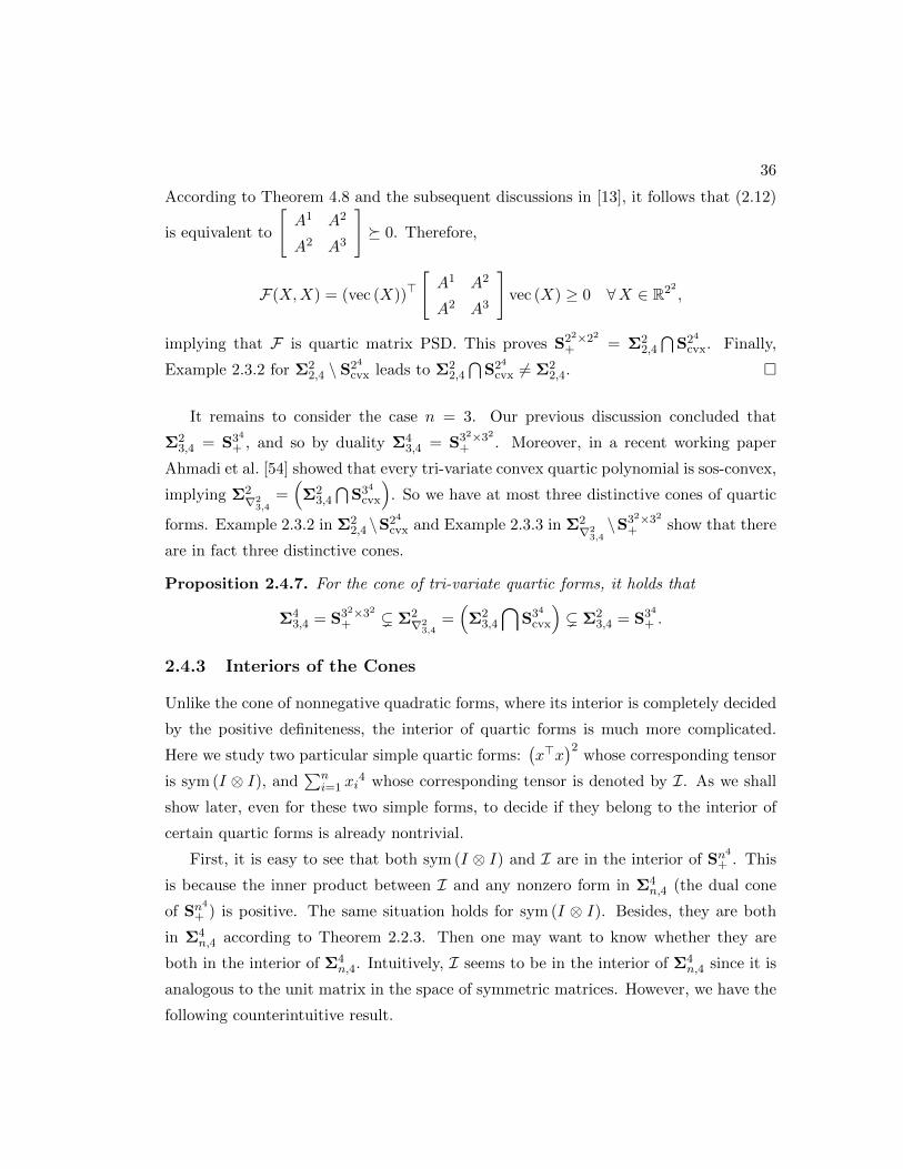
According to Theorem 4.8 and the subsequent discussions in [13], it follows that (2.12)

is equivalent to

[A1 A2

A2 A3

] 0. Therefore,

F(X,X) = (vec (X))>[A1 A2

A2 A3

]vec (X) ≥ 0 ∀X ∈ R22

,

implying that F is quartic matrix PSD. This proves S22×22

+ = Σ22,4

⋂S24

cvx. Finally,

Example 2.3.2 for Σ22,4 \ S24

cvx leads to Σ22,4

⋂S24

cvx 6= Σ22,4.

It remains to consider the case n = 3. Our previous discussion concluded that

Σ23,4 = S34

+ , and so by duality Σ43,4 = S32×32

+ . Moreover, in a recent working paper

Ahmadi et al. [54] showed that every tri-variate convex quartic polynomial is sos-convex,

implying Σ2∇2

3,4=(Σ2

3,4

⋂S34

cvx

). So we have at most three distinctive cones of quartic

forms. Example 2.3.2 in Σ22,4 \S24

cvx and Example 2.3.3 in Σ2∇2

3,4\S32×32

+ show that there

are in fact three distinctive cones.

Proposition 2.4.7. For the cone of tri-variate quartic forms, it holds that

Σ43,4 = S32×32

+ ( Σ2∇2

3,4=(Σ2

3,4

⋂S34

cvx

)( Σ2

3,4 = S34

+ .

2.4.3 Interiors of the Cones

Unlike the cone of nonnegative quadratic forms, where its interior is completely decided

by the positive definiteness, the interior of quartic forms is much more complicated.

Here we study two particular simple quartic forms:(x>x

)2whose corresponding tensor

is sym (I ⊗ I), and∑n

i=1 xi4 whose corresponding tensor is denoted by I. As we shall

show later, even for these two simple forms, to decide if they belong to the interior of

certain quartic forms is already nontrivial.

First, it is easy to see that both sym (I ⊗ I) and I are in the interior of Sn4

+ . This

is because the inner product between I and any nonzero form in Σ4n,4 (the dual cone

of Sn4

+ ) is positive. The same situation holds for sym (I ⊗ I). Besides, they are both

in Σ4n,4 according to Theorem 2.2.3. Then one may want to know whether they are

both in the interior of Σ4n,4. Intuitively, I seems to be in the interior of Σ4

n,4 since it is

analogous to the unit matrix in the space of symmetric matrices. However, we have the

following counterintuitive result.

37

Proposition 2.4.8. It holds that sym (I ⊗ I) ∈ Int (Sn2×n2

+ ) and I /∈ Int (Sn2×n2

+ ).

Before providing the proof, let us first discuss the definition of Int (Sn2×n2

+ ). Follow-

ing Definition 2.1.3, one may define a quartic form F ∈ Int (Sn2×n2

+ ) if

F(X,X) > 0 ∀X ∈ Rn2 \O. (2.13)

However, this condition is sufficient but not necessary. Since for any F ∈ Sn4

and

any skewness matrix Y , we have F(Y, Y ) = 0 according to the proof of Lemma 2.2.4,

which leads to empty interior for Sn2×n2

+ if we strictly follow (2.13). Noticing that

Sn2×n2

+ =F ∈ Sn

4 | F(X,X) ≥ 0, ∀ X ∈ Sn2

by Theorem 2.2.3, the interior of Sn2×n2

+

shall be correctly defined as follows, which is easy to verify by checking the standard

definition of the cone interior.

Definition 2.4.9. A quartic form F ∈ Int (Sn2×n2

+ ) if and only if F(X,X) > 0 for any

X ∈ Sn2 \O.

Proof of Proposition 2.4.8. For any X ∈ Sn2 \O, we observe that sym (I ⊗ I)(X,X) =

2(tr (X))2 + 4 tr (XX>) > 0, implying that sym (I ⊗ I) ∈ Int (Sn2×n2

+ ).

To prove the second part, we let Y ∈ Sn2 \ O with diag (Y ) = 0. Then we have

I(Y, Y ) =∑n

i=1 Y2ii = 0, implying that I /∈ Int (Sn

2×n2

+ ).

Our main result in this subsection are the follow theorems, which exactly indicate Iand sym (I ⊗ I) in the interior of a particular cone in the hierarchy (2.10), respectively.

Theorem 2.4.10. It holds that I /∈ Int (Sn4

cvx) and I ∈ Int (Σ2n,4).

Proof. To prove the first part, we denote quartic form Fε to be Fε(x, x, x, x) =∑n

i=1 x4i−

εx21x

22, which is perturbed from I. By Proposition 2.3.4, Fε ∈ Sn

4

cvx if an only if

Fε(x, x, y, y) =

n∑i=1

x2i y

2i −

ε

6

(x2

1y22 + x2

2y21 + 4x1x2y1y2

)≥ 0 ∀x, y ∈ Rn.

However, choosing x = (1, 0, 0, . . . , 0) and y = (0, 1, 0, . . . , 0) leads to Fε(x, x, y, y) =

− ε6 < 0 for any ε > 0. Therefore Fε /∈ Sn

4

cvx, implying that I 6∈ Int (Sn4

cvx).

For the second part, recall that the dual cone of Σ2n,4 is Sn

2×n2

+ . It suffices to show

that I · F > 0 for any F ∈ Sn2×n2

+ \O, or equivalently I · F = 0 for F ∈ Sn2×n2

+ implies

38

F = O. Now rewrite F as an n2×n2 symmetric matrix MF . Clearly, F ∈ Sn2×n2

+ implies

MF 0, with its diagonal components Fijij ≥ 0 for any i, j, in particular Fiiii ≥ 0 for

any i. Combing this fact and the assumption that I ·F =∑n

i=1Fiiii = 0 yeilds Fiiii = 0

for any i. Next, we noticed that for any i 6= j, the matrix

[Fiiii FiijjFjjii Fjjjj

]is a principle

minor of the positive semidefinite matrix MF ; as a result Fiijj = 0 for any i 6= j. Since

F is super-symmetric, we further have Fijij = Fiijj = 0. Therefore diag (MF ) = 0,

which combining MF 0 leads to MF = O. Hence F = O and the conclusion follows.

Theorem 2.4.11. It holds that sym (I ⊗ I) ∈ Int (Σ4n,4).

Proof. By the duality relationship between Σ4n,4 and Sn

4

+ , it suffices to show that any

F ∈ Sn4

+ with sym (I ⊗ I) · F = 0 implies F = O. For this qualified F , we have

F(x, x, x, x) ≥ 0 for any x ∈ Rn. For any given i, let xi = 1 and other entries be zeros,

and it leads to

Fiiii ≥ 0 ∀ i. (2.14)

Next, let ξ ∈ Rn whose entries are i.i.d. symmetric Bernoulli random variables, i.e.,

Prob ξi = 1 = Prob ξi = −1 = 12 for all i. Then it is easy to compute

E[F(ξ, ξ, ξ, ξ)] =

n∑i=1

Fiiii + 6∑

1≤i<j≤nFiijj ≥ 0. (2.15)

Besides, for any given i 6= j, let η ∈ Rn where ηi and ηj are independent symmetric

Bernoulli random variables and other entries are zeros. Then

E[F(η, η, η, η)] = Fiiii + Fjjjj + 6Fiijj ≥ 0 ∀ i 6= j. (2.16)

Since we assume sym (I ⊗ I) · F = 0, it follows that

n∑i=1

Fiiii + 2∑

1≤i<j≤nFiijj =

1

3

n∑i=1

Fiiii + 6∑

1≤i<j≤nFiijj

+2

3

n∑i=1

Fiiii = 0. (2.17)

Combining (2.14), (2.15) and (2.17), we get

Fiiii = 0 ∀ i. (2.18)

39

It further leads to Fiijj ≥ 0 for any i 6= j by (2.16). Combining this result again

with (2.17) and (2.18), we get

Fiijj = 0 ∀ i 6= j. (2.19)

Now it suffices to prove Fiiij = 0 for all i 6= j, Fiijk = 0 for all distinctive i, j, k, and

Fijk` = 0 for all distinctive i, j, k, `. To this end, for any given i 6= j, let x ∈ Rn where

xi = t2 and xj = 1t and other entries are zeros. By (2.18) and (2.19), it follows that

F(x, x, x, x) = 4Fiiij x3ixj + 4Fijjj xix3

j = 4Fiiij t5 + 4Fijjj/t ≥ 0 ∀ i 6= j.

Letting t→ ±∞, we get

Fiiij = 0 ∀ i 6= j. (2.20)

For any given distinctive i, j, k, let x ∈ Rn whose only nonzero entries are xi, xj and

xk, and we have

F(x, x, x, x) = 12Fiijk x2ixjxk+12Fjjik x2

jxixk+12Fkkij x2kxixj ≥ 0 ∀ distincive i, j, k.

Taking xj = 1, xk = ±1 in the above leads to ±(Fiijk x2i + Fjjik xi) + Fkkij xi ≥ 0 for

any xi ∈ R, and we get

Fiijk = 0 ∀ distincive i, j, k. (2.21)

Finally, for any given distinctive i, j, k, `, let x ∈ Rn whose only nonzero entries are xi,

xj , xk and x`, and we have

F(x, x, x, x) = 24Fijk` xixjxkx` ≥ 0 ∀ distincive i, j, k, `.

Taking xi = xj = xk = 1 and x` = ±1 leads to

Fijk` = 0 ∀ distincive i, j, k, `. (2.22)

Combining equations (2.18), (2.19), (2.20), (2.21) and (2.22) yields F = O.

2.5 Quartic Conic Programming

The study of quartic forms in the previous sections gives rise some new modeling op-

portunities. In this section we shall discuss quartic conic programming, i.e., optimizing

40

a linear function over the intersection of an affine subspace and a cone of quartic forms.

In particular, we shall investigate the following quartic conic programming model:

(QCP ) max C • Xs.t. Ai • X = bi, i = 1, . . . ,m

X ∈ Σ4n,4,

where C,Ai ∈ Sn4

and bi ∈ R for i = 1, . . . ,m. As we will see later, a large class of

non-convex quartic polynomial optimization models can be formulated as a special class

of (QCP ). In fact we will study a few concrete examples to show the modeling power

of the quartic forms that we introduced.

2.5.1 Quartic Polynomial Optimization

Quartic polynomial optimization received much attention in the recent years; see e.g. [22,

32, 33, 34, 36, 59]. Essentially, all the models studied involve optimization of a quartic

polynomial function subject to some linear and/or homogenous quadratic constraints,

including spherical constraints, binary constraints, the intersection of co-centered ellip-

soids, and so on. Below we consider a very general quartic polynomial optimization

model:(P ) max p(x)

s.t. (ai)>x = bi, i = 1, . . . ,m

x>Ajx = cj , j = 1, . . . , l

x ∈ Rn,

where p(x) is a general inhomogeneous quartic polynomial function.

We first homogenize p(x) by introducing a new homogenizing variable, say xn+1,

which is set to one, and get a homogeneous quartic form

p(x) = F(x, x, x, x) = F • (x⊗ x⊗ x⊗ x) ,

where F ∈ S(n+1)4, x =

(x

xn+1

)and xn+1 = 1. By adding some redundant constraints,

41

we have an equivalent formulation of (P ):

max F (x, x, x, x)

s.t. (ai)>x = bi,((ai)>x

)2= bi

2,((ai)>x

)4= bi

4, i = 1, . . . ,m

x>Ajx = cj ,(x>Ajx

)2= cj

2, j = 1, . . . , l

x =

(x

1

)∈ Rn+1.

The objective function of the above problem can be taken as a linear function of

x⊗ x⊗ x⊗ x, and we introduce new variables of a super-symmetric fourth order tensor

X ∈ S(n+1)4. The notations x, X, and X extract part of the entries of X , which are

defined as:x ∈ Rn xi = Xi,n+1,n+1,n+1 ∀ 1 ≤ i ≤ n,X ∈ Sn

2Xi,j = Xi,j,n+1,n+1 ∀ 1 ≤ i, j ≤ n,

X ∈ Sn4 Xi,j,k,` = Xi,j,k,` ∀ 1 ≤ i, j, k, ` ≤ n.

Essentially they can be treated as linear constraints on X . Now by taking X = x⊗ x⊗x ⊗ x, X = x ⊗ x ⊗ x ⊗ x, and X = x ⊗ x, we may equivalently represent the above

problem as a quartic conic programming model with a rank-one constraint:

(Q) max F • Xs.t. (ai)>x = bi, (ai ⊗ ai) •X = bi

2, (ai ⊗ ai ⊗ ai ⊗ ai) • X = bi4, i = 1, . . . ,m

Aj •X = cj , (Aj ⊗Aj) • X = cj2, j = 1, . . . , l

Xn+1,n+1,n+1,n+1 = 1, X ∈ Σ4n+1,4, rank (X ) = 1.

Dropping the rank-one constraint, we obtain a relaxation problem, which is exactly in

the form of quartic conic program (QCP ):

(RQ) max F • Xs.t. (ai)>x = bi, (ai ⊗ ai) •X = bi

2, (ai ⊗ ai ⊗ ai ⊗ ai) • X = bi4, i = 1, . . . ,m

Aj •X = cj , (Aj ⊗Aj) • X = cj2, j = 1, . . . , l

Xn+1,n+1,n+1,n+1 = 1, X ∈ Σ4n+1,4.

Interestingly, the relaxation from (Q) to (RQ) is not lossy; or, to put it differently,

(RQ) is a tight relaxation of (Q), under some mild conditions.

Theorem 2.5.1. If Aj ∈ Sn2

+ for all 1 ≤ j ≤ l in the model (P ), then (RQ) is

equivalent to (P ) in the sense that: (i) they have the same optimal value; (ii) if X is

42

optimal to (RQ), then x is in the convex hull of the optimal solution of (P ). Moreover,

the minimization counterpart of (P ) is also equivalent to the minimization counterpart

of (RQ).

Theorem 2.5.1 shows that (P ) is in fact a conic quartic program (QCP ) when the

matrices Aj ’s in (P ) are positive semidefinite. Notice that the model (P ) actually

includes quadratic inequality constraints x>Ajx ≤ cj as its subclasses, for one can

always add a slack variable yj ∈ R with x>Ajx+ yj2 = cj , while reserving the new data

matrix

[Aj 0

0 1

]in the quadratic term still being positive semidefinite.

As mentioned before, Burer [57] established the equivalence between a large class

of mixed-binary quadratic programs and copositive programs. Theorem 2.5.1 may be

regarded as a quartic extension of Burer’s result. The virtue of this equivalence is to

alleviate the highly non-convex objective and/or constraints of (QCP ) and retain the

problem in convex form, although the difficulty is all absorbed into the dealing of the

quartic cone, which is nonetheless a convex one. Note that this is characteristically

a property for polynomial of degree higher than 2: the SDP relaxation for similar

quadratic models can never be tight.

In the following, we shall present the proof of Theorem 2.5.1. Since the proof for their

minimization counterparts is exactly the same, we only prove the equivalence relation

for the maximization problems. That is, we shall prove the equivalence between (Q)

and (RQ).

To start with, let us first investigate the feasible regions of these two problems, to

be denoted by feas (Q) and feas (RQ) respectively. The relationship between feas (Q)

and feas (RQ) is revealed by the following lemma.

Lemma 2.5.2. It holds that conv (feas (Q)) ⊆ feas (RQ) = conv (feas (Q)) + P, where

P := cone

(x

0

)⊗(x

0

)⊗(x

0

)⊗(x

0

)∣∣∣∣ (ai)>x = 0 ∀ 1 ≤ i ≤ m,x>Ajx = 0 ∀ 1 ≤ j ≤ l

⊂ Σ4

n+1,4.

Proof. First, it is obvious that conv (feas (Q)) ⊆ feas (RQ), since (RQ) is a relaxation

of (Q) and feas (RQ) is convex. Next we notice that the recession cone of feas (RQ) is

43

equal toX ∈ Σ4n+1,4

∣∣∣∣∣∣∣∣Xn+1,n+1,n+1,n+1 = 0,

(ai)>x = 0, (ai ⊗ ai) •X = 0, (ai ⊗ ai ⊗ ai ⊗ ai) • X = 0 ∀ 1 ≤ i ≤ m,Aj •X = 0, (Aj ⊗Aj) • X = 0 ∀ 1 ≤ j ≤ l

.

Observing that X ∈ Σ4n+1,4 and Xn+1,n+1,n+1,n+1 = 0, it is easy to see that x = 0 and

X = 0. Thus the recession cone of feas (RQ) is reduced toX ∈ Σ4n+1,4

∣∣∣∣∣∣∣∣Xn+1,n+1,n+1,n+1 = 0, x = 0, X = 0,

(ai ⊗ ai ⊗ ai ⊗ ai) • X = 0 ∀ 1 ≤ i ≤ m,(Aj ⊗Aj) • X = 0 ∀ 1 ≤ j ≤ l

⊇ P,

which proves feas (RQ) ⊇ conv (feas (Q)) + P.

Finally, we shall show the inverse inclusion, i.e., feas (RQ) ⊆ conv (feas (Q)) + P.

Suppose X ∈ feas (RQ), then it can be decomposed as

X =∑k∈K

(yk

αk

)⊗(yk

αk

)⊗(yk

αk

)⊗(yk

αk

), (2.23)

where αk ∈ R, yk ∈ Rn for all k ∈ K. Immediately we have∑k∈K

αk4 = Xn+1,n+1,n+1,n+1 = 1. (2.24)

Now divide the index set K into two parts, with K0 := k ∈ K | αk = 0 and K1 :=

k ∈ K | αk 6= 0, and let zk = yk/αk for all k ∈ K1. The decomposition (2.23) is then

equivalent to

X =∑k∈K1

αk4

(zk

1

)⊗(zk

1

)⊗(zk

1

)⊗(zk

1

)+∑k∈K0

(yk

0

)⊗(yk

0

)⊗(yk

0

)⊗(yk

0

).

If we can prove that(zk

1

)⊗(zk

1

)⊗(zk

1

)⊗(zk

1

)∈ feas (Q) ∀ k ∈ K1 (2.25)(

yk

0

)⊗(yk

0

)⊗(yk

0

)⊗(yk

0

)∈ P ∀ k ∈ K0 (2.26)

then by (2.24), we shall have X ∈ conv (feas (Q)) + P, proving the inverse inclusion.

44

In the following we shall prove (2.25) and (2.26). Since X ∈ feas (RQ), together

with x =∑

k∈K αk3yk, X =

∑k∈K αk

2yk ⊗ yk, and X =∑

k∈K yk ⊗ yk ⊗ yk ⊗ yk, we

obtain the following equalities:∑k∈K

αk3(ai)>yk = bi,

∑k∈K

αk2(

(ai)>yk)2

= bi2,∑k∈K

((ai)>yk

)4= bi

4, ∀ 1 ≤ i ≤ m

∑k∈K

αk2(yk)>Ajyk = cj ,

∑k∈K

((yk)>Ajyk

)2= cj

2, ∀ 1 ≤ j ≤ l.

As a direct consequence of the above equalities and (2.24), we have(∑k∈K

αk2 · αk(ai)>yk

)2

= bi2 =

(∑k∈K

αk4

)(∑k∈K

αk2(

(ai)>yk)2), ∀ 1 ≤ i ≤ m

(∑k∈K

αk2(

(ai)>yk)2)2

= bi4 =

(∑k∈K

αk4

)(∑k∈K

((ai)>yk

)4), ∀ 1 ≤ i ≤ m

(∑k∈K

αk2(yk)>Ajyk

)2

= cj2 =

(∑k∈K

αk4

)(∑k∈K

((yk)>Ajyk

)2), ∀ 1 ≤ j ≤ l.

Noticing that the equalities hold for the above Cauchy-Schwarz inequalities, it follows

that for every 1 ≤ i ≤ m and every 1 ≤ j ≤ l, there exist δi, εi, θj ∈ R, such that

δiαk2 = αk(a

i)>yk, εiαk2 =

((ai)>yk

)2and θjαk

2 = (yk)>Ajyk ∀ k ∈ K. (2.27)

If αk = 0, then (ai)>yk = 0 and (yk)>Ajyk = 0, which implies (2.26). Moreover, due

to (2.27) and (2.24),

δi = δi

(∑k∈K

αk4

)=∑k∈K

δiαk2 · αk2 =

∑k∈K

αk(ai)>yk · αk2 = bi ∀ 1 ≤ i ≤ m.

Similarly, we have θj = cj for all 1 ≤ j ≤ l. If αk 6= 0, noticing zk = yk/αk, it follows

from (2.27) that

(ai)>zk = (ai)>yk/αk = δi = bi ∀ 1 ≤ i ≤ m

(zk)>Ajzk = (yk)>Ajyk/αk2 = θj = cj ∀ 1 ≤ j ≤ l,

which implies (2.25).

45

Proof of Theorem 2.5.1: we notice that if Aj is positive semidefinite, then

x>Ajx = 0 ⇐⇒ Ajx = 0. Therefore,

(x

0

)⊗(x

0

)⊗(x

0

)⊗(x

0

)∈ P implies that

x is a recession direction of the feasible region for (P ). With this property and using a

similar argument of Theorem 2.6 in [57], Theorem 2.5.1 follows immediately.

2.5.2 Biquadratic Assignment Problems

The biquadratic assignment problem (BQAP ) is a generalization of the quadratic as-

signment problem (QAP ), which is to minimize a quartic polynomial of an assignment

matrix:(BQAP ) min

∑1≤i,j,k,`,s,t,u,v≤nAijk`BstuvXisXjtXkuX`v

s.t.∑n

i=1Xij = 1, j = 1, . . . , n∑nj=1Xij = 1, i = 1, . . . , n

Xij ∈ 0, 1, i, j = 1, . . . , n

X ∈ Rn2,

where A,B ∈ Rn4. This problem was first considered by Burkard et al. [60] and was

shown to have applications in the VLSI synthesis problem. After that, several heuristics

for (BQAP ) were developed by Burkard and Cela [61], and Mavridou et al. [62].

In this subsection we shall show that (BQAP ) can be formulated as a quartic conic

program (QCP ). First notice that the objective function of (BQAP ) is a fourth order

polynomial function with respect to the variables Xij ’s, where X is taken as an n2-

dimensional vector. The assignment constraints∑n

i=1Xij = 1 and∑n

j=1Xij = 1 are

clearly linear equality constraints. Finally by imposing a new variable x0 ∈ R, and the

binary constraints Xij ∈ 0, 1 is equivalent to(Xij

x0

)> [ 1 −1

−1 1

](Xij

x0

)=

1

4and x0 =

1

2,

where the coefficient matrix in the quadratic term is indeed positive semidefinite. Ap-

plying Theorem 2.5.1 we have the following result:

Corollary 2.5.3. The biquadratic assignment problem (BQAP ) can be formulated as

a quartic conic program (QCP ).

46

2.5.3 Eigenvalues of Fourth Order Super-Symmetric Tensor

The notion of eigenvalue for matrices has been extended to tensors, proposed by Lim [63]

and Qi [64] independently. Versatile extensions turned out to be possible, among which

the most popular one is called Z-eigenvalue (in the notion by Qi [64]). Restricting to

the space of fourth order super-symmetric tensors Sn4, λ ∈ R is called a Z-eigenvalue of

the super-symmetric tensor F ∈ Sn4, if the following system holdsF(x, x, x, ·) = λx,

x>x = 1,

where x ∈ Rn is the corresponding eigenvector with respect to λ. Notice that the Z-

eigenvalues are the usual eigenvalues for a symmetric matrix, when restricting to the

space of symmetric matrices Sn2. We refer interested readers to [63, 64] for various

other definitions of tensor eigenvalues and [65] for their applications in polynomial op-

timizations.

Observe that x is a Z-eigenvector of the fourth order tenor F if and only if x is a

KKT point to following polynomial optimization problem:

(E) max F(x, x, x, x)

s.t. x>x = 1.

Furthermore, x is the Z-eigenvector with respect to the largest (resp. smallest) Z-

eigenvalue of F if and only if x is optimal to (E) (resp. the minimization counterpart

of (E)). As the quadratic constraint x>x = 1 satisfies the condition in Theorem 2.5.1,

we reach the following conclusion:

Corollary 2.5.4. The problem of finding a Z-eigenvector with respect to the largest or

smallest Z-eigenvalue of a fourth order super-symmetric tensor F can be formulated as

a quartic conic program (QCP ).

To conclude this section, as well as the whole chapter, we remark here that quartic

conic problems have many potential application, alongside their many intriguing theo-

retical properties. The hierarchical structure of the quartic cones that we proved in the

previous sections paves a way for possible relaxation methods to be viable. For instance,

according to the hierarchy relationship (2.10), by relaxing the cone Σ4n,4 to an easy cone

47

Sn2×n2

+ lends a hand to solve the quartic conic problem approximately. The quality of

such solution methods and possible enhancements remain our future research topic.

Chapter 3

Polynomial Sized Representation

of Hilbert’s Identity

3.1 Introduction

The so-called Liouville formula states that

(x21 + x2

2 + x23 + x2

4)2 =1

6

∑1≤i<j≤4

(xi + xj)4 +

1

6

∑1≤i<j≤4

(xi − xj)4, (3.1)

which is straightforward to verify. Interestingly, such ‘rank-one’ decomposition of the

positive quartic form can be extended, giving rise to an identity known as Hilbert’s

identity, which asserts that for any fixed positive integers d and n, there always exist

real vectors a1, a2, ..., at ∈ Rn such that

(x>x)d =t∑i=1

(a>i x)2d, (3.2)

for any x ∈ Rn. It worths mentioning that Hilbert’s identity is a fundamental result

in mathematics. As we mentioned at the very beginning of this thesis, Reznick [16]

managed to solve Hilbert’s seventeenth problem constructively when the polynomial

function is positive definite. Moreover, this identity can be readily extended to a more

general setting. For any given A 0, by letting y = A12x and applying (3.2), one has

(x>Ax)2 = (y>y)2 =t∑

j=1

((bj)>y

)2d=

t∑j=1

((bj)>A

12x)2d

,

48

49

which guarantees the existence of vectors a1, a2, · · · , at ∈ Rn with aj = A12 bj for j =

1, 2, . . . , t such that

(x>Ax)d =t∑

j=1

((aj)>x

)2d. (3.3)

(3.2) was first proved by Hilbert (see [17]), and he showed that

Given fixed positive integers d and n, there exist 2d + 1 real numbers

β1, β2, · · · , β2d+1, 2d+ 1 positive real numbers ρ1, ρ2, · · · , ρ2d+1, and a posi-

tive real number αd, such that

(x>x)d =1

αd

n∑i1=1

n∑i2=1

· · ·n∑

i2d+1=1

ρi1ρi2 · · · ρi2d+1(βi1x1+βi2x2+· · ·+βi2d+1

xi2d+1)2d.

(3.4)

It is obvious that the number of 2d-powered linear terms on the right hand side of (3.4)

is (2d + 1)n, which is exponential with respect to n and thus inefficient for practical

purposes. In general, the presentation of (x>x)d is not unique. For example, one may

verify that

(x21+x2

2+x23)2 =

1

3

3∑i=1

x4i+

1

3

∑1≤i<j≤3

∑βj=±1

(xi+βjxj)4 =

2

3

3∑i=1

x4i+

1

3

∑β2=±1β3=±1

(x1+β2x2+β3x3)4,

which leads to two different representations of the form (x21 + x2

2 + x23)2. An interesting

question is to find a succinct (preferably the shortest) representation among all the dif-

ferent representations, including the one from Hilbert’s construction. By Caratheodory’s

theorem, there exists a decomposition such that the value of t in (3.2) is no more than(n+2d−1

2d

)+ 1. Unfortunately, Caratheodory’s theorem is non-constructive. This moti-

vates us to construct a polynomial-size representation, i.e., t = O(nk) for some constant

k in (3.2).

Toward this end, let’s first reinvestigate the construction (3.4) given by Hilbert.

Define i.i.d. random variables ξ1, ξ2, · · · , ξn with supporting set ∆ = β1, β2, · · · , β2d+1,and let Prob (ξk = βi) = ρi

γdfor all 1 ≤ i ≤ 2d+ 1 and 1 ≤ k ≤ n, where γd =

∑2d+1i=1 βi.

50

Then identity (3.4) is equivalent to

(x>x)d =γddαd

E

n∑j=1

ξjxj

2d =

γddαd

∑p∈Pn2d

E

n∏j=1

ξpjj

n∏j=1

xpjj

=γddαd

∑p∈Pn2d

n∏j=1

E[ξpjj

] n∏j=1

xpjj , (3.5)

where Pnk :=

(p1, p2, · · · , pn)> ∈ Zn+ | p1 + p2 + · · ·+ pn = k

. In light of formula (3.5),

we learn that the length of representation of (x>x)d equals to the size of sample space

spanned by random variables ξ1, ξ2, · · · , ξn and there are (2d+ 1)n possible outcomes in

total. As a consequence, the issue of reducing the representation of (x>x)d boils down

whether we can find another n random variables η1, η2, · · · , ηn with smaller sample space

such that

(x>x)d =γddαd

E

n∑j=1

ξjxj

2d =

γddαd

E

n∑j=1

ηjxj

2d . (3.6)

This issue will be particularly addressed in Section 3.2 and a key concept called

k-wise zero-correlation will also be introduced there. Then we discuss how to construct

k-wise zero-correlated random variables in Section 3.3, and find the polynomial sized

representation of Hilbert’s identity in Section 3.4. Finally, in Section 3.5 we conclude

this chapter with an application of showing the matrix 2 7→ 4 norm problem, whose

computational complexity was previously, is actually NP-hard unknown.

3.2 k-Wise Zero-Correlation Random Variables

In this section, let us first introduce the new notion of k-wise uncorrelated random

variables, which may appear to be completely unrelated to the discussion of Hilbert’s

identity at first glance.

Definition 3.2.1. (k-wise zero-correlation) A set of random variables ξ1, ξ2, · · · , ξnis called k-wise zero-correlated if

E

n∏j=1

ξpjj

=

n∏j=1

E[ξpjj

]∀ p1, p2, · · · , pn ∈ Z+ with

n∑i=1

pi = k. (3.7)

51

To relate this definition to our Hilbert’s identity, we consider 2d-wise uncorrelated

random variables η1, η2, · · · , ηn, where each one is identical to ξ1 in (3.5). Therefore, we

have E[ηpj

]= E [ξp1 ] and E

[∏nj=1 η

pjj

]=∏nj=1 E

[ηpjj

]∀ p ∈ Pn2d, which lead to (3.6). In

other words, η1, η2, · · · , ηn constitute another representation of Hilbert’s identity. We

summarize this result in the following result as preparation for the later discussion.

Proposition 3.2.2. If ξ1, ξ2, · · · , ξn are i.i.d. random variables, and η1, η2, · · · , ηn are

2d-wise zero-correlated, satisfying the moments constraints E[ηpj

]= E [ξp1 ] for all 0 <

p ≤ 2d and 1 ≤ j ≤ n, then E

[(∑nj=1 ξjxj

)2d]

= E

[(∑nj=1 ηjxj

)2d]

.

Now we can see that the key of reducing the length of representation in (3.2) is to

construct 2d-wise zero-correlated random variables satisfying certain moments condi-

tions, such that the sample space is as small as possible.

Before addressing the issue of finding such random variables, below we shall first

discuss a related notion known as k-wise independence.

Definition 3.2.3. (k-wise independence) A set of random variables Ξ = ξ1, ξ2, · · · , ξnwith each taking values on the set ∆ = δ1, δ2, · · · , δq is called k-wise independent, if

any k different random variables ξi1 , ξi2 , · · · , ξik of Ξ are independent, i.e.,

Prob ξi1 = δi1 , ξi2 = δi2 , · · · , ξik = δik =

k∏j=1

Probξij = δij

∀ δij ∈ ∆, j = 1, 2, . . . , k.

Note that when k = 2, k-wise independence is usually called pair-wise independence.

Since 1980’s, k-wise independence has been a popular topic in theoretical computer

science. Essentially, working with k-wise independence (instead of the full independence)

means that one can reduce the size of the sample space in question. In many cases, this

feature is crucial. For instance, when ∆ = 0, 1 and Prob ξ1 = 0 = Prob ξ1 = 1 =12 , Alon, Babai, and Itai [66] constructed a sample space of size being approximately

nk2 . For the same ∆, when ξ1, ξ2, · · · , ξn are independent but not identical, Karloff and

Mansour [67] proved that the size of sample space can be upper bounded by O(nk).

In the case of ∆ = 0, 1, . . . , q − 1 with q being a prime number, the total number

of random variables being k-wise independent are quite restricted. For given k < q,

Joffe [68] showed that there are up to q+1 random variables form a k-wise independent

set and the size of the sample space is qk.

52

Clearly, k-wise independence implies k-wise zero-correlation. Therefore, we may ap-

ply the existing results of k-wise independence to get k-wise zero-correlation random

variables. However, the afore-mentioned constructions of k-wise independent random

variables heavily depend on the structure of ∆ (e.g., it requires that |∆| = 2 or k < |∆|).Moreover, the construction of k-wise independent random variables is typically compli-

cated and technically involved (see [67]). In fact, for certain problems (e.g., polynomial-

size representation of Hilbert’s identity in this case), we only need the random variables

to be k-wise zero-correlated. Therefore in next section, we propose a tailor-made sim-

ple construction which suits the structure of k-wise zero-correlation random variables.

As we shall see later, our approach can handle more general setting of the following

supporting set

∆q := 1, ωq, · · · , ωq−1q , with ωq = e

i 2πq = cos

2π

q+ i sin

2π

qand q is prime, (3.8)

and k can be any parameter. Conceptually, our approach is rather generic: the k-wise

zero-correlated random variables are constructed based only on the product of a small

set of i.i.d. random variables with their powers; the sample space would be polynomial-

size if the number of such i.i.d. random variables is O(log n).

3.3 Construction of k-wise Zero-Correlated Random Vari-

ables

In this section, we shall construct k-wise zero-correlated random variables, which are

identical and uniformly distributed on ∆q defined by (3.8). The rough idea is as follows.

We first generate m i.i.d. random variables ξ1, ξ2, · · · , ξm, based on which we can define

new random variables η1, η2, · · · , ηn such that ηi :=∏

1≤j≤m ξcijj for i = 1, 2, . . . , n.

Therefore, the size of sample space of η1, η2, · · · , ηn is bounded above by qm, which

yields a polynomial-size space if we let m = O(logq n). The remaining part of this

section is devoted to the discussion of the property for the power indices cij ’s, in order

to guarantee η1, η2, · · · , ηn to be k-wise zero-correlated, and how to find those power

indices.

53

3.3.1 k-wise Regular Sequence

Let us start with a couple of notations and definitions for the preparation. Sup-

pose c is a number with m digits and c[`] is the value of its `-th bit. We call c

to be endowed with the base q, if c[`] ∈ 0, 1, . . . , q − 1 for all 1 ≤ ` ≤ m. In

other words, c =∑m

`=1 c[`]q`−1. Recall we have defined a subset Pnk ⊆ Zn+ to be

(p1, p2, · · · , pn)> ∈ Zn+ | p1 + p2 + · · ·+ pn = k

. Then for any given prime number

q, we define another set associated with q below

Pnk(q) := p ∈ Pnk | ∃ i (1 ≤ i ≤ n) such that q - pi .

It is easy to see that |Pnk(q)| ≤ |Pnk | =(n+k−1

k

).

Now we can define the concept of k-wise regular sequence as follows.

Definition 3.3.1. A sequence of m digits numbers c1, c2, · · · , cn of base q is called

k-wise regular if for any p ∈ Pnk(q), there exists ` (1 ≤ ` ≤ m) such that

n∑j=1

pj · cj [`] 6= 0 mod q.

Why are we interested in such regular sequences? The answer lies in the following

proposition.

Proposition 3.3.2. Suppose m digits numbers c1, c2, · · · , cn of base q are k-wise reg-

ular, where q is a prime number, and ξ1, ξ2, · · · , ξm are i.i.d. random variables uniformly

distributed on ∆q. Then η1, η2, · · · , ηn with

ηi :=∏

1≤`≤mξci[`]` , i = 1, 2, · · · , n (3.9)

are k-wise zero-correlated.

Proof. Let η1, η2, · · · , ηn be defined as in (3.9). As ξi is uniformly distributed on ∆q for

1 ≤ i ≤ m and q is prime, we have

E[ξpi ] = E[ηpj

]=

1, if q | p,0, otherwise.

54

For any given p ∈ Pnk , if q | pi for all 1 ≤ i ≤ n, then

E

n∏j=1

ηpjj

= E

∏1≤`≤m

ξp1·c1[`]`

∏1≤`≤m

ξp2·c2[`]`

· · · ∏

1≤`≤mξpn·cn[`]`

=

∏1≤`≤m

E[ξ∑nj=1 pj ·cj [`]

`

]= 1 =

n∏j=1

E[ηpjj

].

Otherwise, there exists some i such that q - pi (in this case p ∈ Pnk(q)), which implies

that E [ηpii ] = 0. Moreover by k-wise regularity, we can find some `0 satisfying∑n

j=1 pj ·cj [`0] 6= 0 mod q. Therefore

E

n∏j=1

ηpjj

=∏

1≤`≤mE[ξ∑nj=1 pj ·cj [`]

`

]= 0 =

n∏j=1

E[ηpjj

],

and the conclusion follows.

3.3.2 A Randomized Algorithm

We shall now focus on how to find such k-wise regular sequence c1, c2, · · · , cn of base

q. First, we present a randomized process, in which ci[`] is randomly and uniformly

chosen from 0, 1, . . . , q − 1 for all 1 ≤ i ≤ n and 1 ≤ ` ≤ m. The algorithm is as

follows.

Algorithm RAN

Input: Dimension n and m := dk logq ne.Output: A sequence c1, c2, · · · , cn in m digits of base q.

Step 0: Construct S = (0, · · · , 0, 0︸︷︷︸m

), (0, · · · , 0, 1︸︷︷︸m

), · · · , (q − 1, · · · , q − 1︸︷︷︸m

) of base q.

Step 1: Independently and uniformly take ci ∈ S for i = 1, 2, . . . , n.

Step 2: Assemble the sequence c1, c2, · · · , cn and exit.

Theorem 3.3.3. If 1 < k < n and q is a prime number, then Algorithm RAN

returns a k-wise m-digit regular sequence c1, c2, · · · , cn of base q with probability at

least 1− (1.5)k−1

k! , which is independent of n and q.

55

Proof. Since c1, c2, · · · , cn is a sequence of m-digit numbers of base q, if it is not

regular, then there exist p ∈ Pnk , such that

n∑j=1

pj · cj [`] = 0 mod q ∀ 1 ≤ ` ≤ m.

Therefore, we have

Prob c1, c2, · · · , cn is not k-wise regular

≤∑

p∈Pnk (q)

Prob

n∑j=1

pj · cj [`] = 0 mod q, ∀ 1 ≤ ` ≤ m

.

For any given p ∈ Pnk(q), we may without loss of generality assume that q - pn. If

we fix c1, c2, · · · , cn−1, as q is prime, then there is only one solution for cn such that∑nj=1 pj · cj [`] = 0 mod q,∀ 1 ≤ ` ≤ m. Combining the fact that c1, c2, · · · , cn are

independently and uniformly generated, we have

Prob

n∑j=1

pj · cj [`] = 0 mod q, ∀ 1 ≤ ` ≤ m

= Prob

n∑j=1

pj · cj [`] = 0 mod q, ∀ 1 ≤ ` ≤ m∣∣∣∣ c1 = d1, c2 = d2, · · · , cn−1 = dn−1

·∑d1,d2,··· ,dn−1∈S

Prob c1 = d1, c2 = d2, · · · , cn−1 = dn−1

=1

qm

∑d1,d2,··· ,dn−1∈S

Prob c1 = d1, c2 = d2, · · · , cn−1 = dn−1

≤ 1

nk. (3.10)

Finally,

Prob c1, c2, · · · , cn is k-wise regular

= 1− Prob c1, c2, · · · , cn is not k-wise regular

≥ 1− |Pnk(q)| · 1

nk≥ 1− |Pnk | ·

1

nk= 1−

(n+ k − 1

k

)· 1

nk≥ 1− (1.5)k−1

k!.

56

For some special q and k, in particular relating to the the simplest case of Hilbert’s

identity (4-wise regular sequence of base 2), the lower bound of the probability in The-

orem 3.3.3 can be improved.

Proposition 3.3.4. If k = 4 and q = 2, then Algorithm RAN returns a 4-wise

regular sequence c1, c2, · · · , cn of base 2 with probability at least 1− 12n2 − 1

4! .

The proof is similar to that of Theorem 3.3.3, and thus is omitted.

3.3.3 De-Randomization

Although k-wise regular sequence always exists and can be found with high probability,

one may however wish to construct such regular sequence deterministically. In fact, this

is possible if we apply Theorem 3.3.3 in a slightly different manner, which is shown in

the following algorithm. Basically, we first start with a small size of regular set C, and

enumerate all the remaining numbers in order to find c such that C∪c is also regular.

Updating C with C ∪ c, and repeat this procedure until the cardinality of C reaches

n. Moreover, thanks to the polynomial-size sample space, this ‘brutal force’ approach

still runs in polynomial-time.

Algorithm DET

Input: Dimension n and m := dk logq ne.Output: A sequence c1, c2, · · · , cn in m digits of base q.

Step 0: Construct S = (0, · · · , 0, 0︸︷︷︸m

), (0, · · · , 0, 1︸︷︷︸m

), · · · , (q − 1, · · · , q − 1︸︷︷︸m

) of base q,

and a sequence C := c1, c2, · · · , ck in m digits, where

ci := (0, · · · , 0, 1, 0, · · · , 0︸︷︷︸k−1

) for i = 1, 2, . . . , k. Let the index count be τ := k.

Step 1: If τ = n, then go to Step 2; Otherwise enumerate S \ C to find a c ∈ S \ Csuch that C ∪ c is k-wise regular. Let cτ+1 := c, C := C ∪ cτ+1and τ := τ + 1, and return to Step 1.

Step 2: Assemble the sequence c1, c2, · · · , cn and exit.

It is obvious that the initial sequence c1, c2, · · · , ck is k-wise regular. In order for

Algorithm DET to exit successfully, it remains to argue that it is always possible to

57

expand the k-wise regular sequence by one in Step 1, as long as τ < n.

Theorem 3.3.5. Suppose that 3 ≤ k ≤ τ < n, q is a prime number, and C with |C| = τ

is k-wise regular. If we uniformly pick cτ+1 from S, then

Prob C ∪ cτ+1 is k-wise regular ≥ 1− (1.5)k

k!

(τ + 1

n

)k,

ensuring that cτ+1 ∈ S | C ∪ cτ+1 is k-wise regular 6= ∅.

Proof. Like in the proof of Theorem 3.3.3, we have

Prob C ∪ cτ+1 is not k-wise regular

≤∑

p∈Pτ+1k (q)

Prob

τ+1∑j=1

pj · cj [`] = 0 mod q, ∀ 1 ≤ ` ≤ m

.

For any p ∈ Pτ+1k (q), since q is prime, by using a similar argument as of (5.4), we can

get

Prob

τ+1∑j=1

pj · cj [`] = 0 mod q, ∀ 1 ≤ ` ≤ m

≤ 1

nk.

Therefore,

Prob C ∪ cτ+1 is k-wise regular ≥ 1−∣∣Pτ+1k (q)

∣∣ 1

nk≥ 1−

(τ + k

k

)1

nk

≥ 1− (1.5)k

k!

(τ + 1

n

)k> 0.

By the above theorem, Step 1 of Algorithm DET guarantees to expand k-wise

regular sequence of base q before reaching the desired cardinality τ = n. A straight-

forward computation shows that Algorithm DET requires an overall complexity of

O(n2k−1 logq n).

3.4 Polynomial-Size Representation of Hilbert’s Identity

3.4.1 Polynomial-Size Representation of Quartic Hilbert’s Identity

Armed with k-wise zero-correlated random variables, we are able to construct polynomial-

size representation of the fourth moments tensor. In Hilbert’s construction (3.5), the

58

supporting set ∆ is too complicated to apply the result in Section 3.3. However as we

mentioned earlier, such decomposition of (3.5) is not unique. In fact, when d = 2, we

observe that

(x>x)2 =

(n∑i=1

x2i

)2

=2

3

n∑i=1

x4i +

1

3E

n∑j=1

ξjxj

4 , (3.11)

where ξ1, ξ2, · · · , ξn are i.i.d. symmetric Bernoulli random variables. Applying either

Algorithm RAN or Algorithm DET leads to a 4-wise regular sequence of base

2, based on which we can define random variables η1, η2, · · · , ηn as we did in (3.9).

Proposition 3.3.2 guarantees that η1, η2, · · · , ηn are 4-wise zero-correlated, and it is easy

to check that

E[ηj ] = E[η3j ] = E[ξ1] = E[ξ3

1 ] = 0, E[η2j ] = E[η4

j ] = E[ξ21 ] = E[ξ4

1 ] = 1 ∀ 1 ≤ j ≤ n.

Thus, by Proposition 3.2.2, we have that E

[(∑nj=1 ηjxj

)4]

= E

[(∑nj=1 ξjxj

)4]. More-

over, the size of sample space of η1, η2, · · · , ηn is at most 2dk logq ne ≤ 2n4, which means

the new representation has at most n+2n4 fourth powered terms leading to the following

main result.

Theorem 3.4.1. Given a positive integer n, we can find τ (≤ 2n4) vectors b1, b2, · · · , bτ ∈Rn in polynomial time, such that

(x>x)2 =2

3

n∑i=1

x4i +

τ∑j=1

((bj)>x

)4∀x ∈ Rn.

In fact, the result above can be extended to a more general setting as follows.

Corollary 3.4.2. Given a positive semidefinite matrix A ∈ Rn×n, we can find τ (≤2n4 + n) vectors a1, a2, · · · , aτ ∈ Rn in polynomial time, such that

(x>Ax)2 =τ∑i=1

((ai)>x

)4∀x ∈ Rn.

Proof. By letting y = A12x and applying Theorem 3.4.1, we can find b1, b2, · · · , bτ in

polynomial time with τ ≤ 2n4, such that

(x>Ax)2 = (y>y)2 =2

3

n∑i=1

y4i +

τ∑j=1

((bj)>y

)4=

n∑i=1

((2

3

) 14

(ei)>A12x

)4

+

τ∑j=1

((bj)>A

12x)4.

59

The conclusion follows by letting ai =(

23

) 14 A

12 ei for i = 1, 2, . . . , n, and ai+n = A

12 bi

for i = 1, 2, . . . , τ .

3.4.2 Polynomial-Size Representation of of qd-th degree Hilbert’s Iden-

tity

In this subsection we are going to generalize the result in Section 3.4.1 to qd-th degree

polynomial. That is for any given positive integers q, d and n, we want to vectors

a1, a2, · · · , at ∈ Rn, such that(n∑i=1

xqi

)d=

t∑j=1

((aj)>x

)qd∀x ∈ Rn. (3.12)

Unfortunately, the above does not hold in general, as the following counter example

shows.

Example 3.4.3. The function f(x) = (x31+x3

2)2 = x61+2x3

1x32+x6

2 cannot be decomposed

in the form of (3.12) with q = 3 and d = 2, i.e., a sum of sixth powered linear terms.

This can be easily proven by contradiction. Suppose we can find a1, a2, · · · , at ∈ Rn,

such that

x61 + 2x3

1x32 + x6

2 =t∑i=1

(aix1 + bix2)6 . (3.13)

There must exist some (aj , bj) with ajbj 6= 0, since otherwise there is no monomial x31x

32

in the right hand side of (3.13). As a consequence, the coefficient of monomial x21x

42 in

the right hand side of (3.13) is at least(

62

)a2jb

4j > 0, which is null on the left side of the

equation, leading to a contradiction.

In the same vein one can actually show that (3.12) cannot hold for any q ≥ 3.

Therefore, we turn to qd-th degree complex polynomial, i.e., both the coefficients and

variables in (3.12) are now allowed to take complex values. Similar to (3.11), we have

the following identity: n∑j=1

xqj

2

=

1− 2(2qq

) n∑

j=1

x2qj +

2(2qq

)E( n∑

i=1

ξixi

)2q , (3.14)

where ξ1, ξ2, · · · , ξn are i.i.d. random variables uniformly distributed on ∆q. Moreover,

we can further prove (3.12) for more general complex case.

60

Proposition 3.4.4. Given any positive integers q and n, there exist a1, a2, · · · , aτ ∈ Cn

such that (n∑i=1

xqi

)2d

=τ∑j=1

((aj)>x

)2dq∀x ∈ Cn. (3.15)

Proof. This proof is based on mathematical induction. The case d = 1 is already guar-

anteed by (3.14). Suppose that (3.15) is true for d−1, then there exist b1, b2, · · · , bt ∈ Cn

such that (n∑i=1

xqi

)2d

=

( n∑i=1

xqi

)2d−12

=

t∑j=1

((bj)>x

)2d−1q

2

.

By applying (3.14) to the above identity, there exist c1, c2, · · · , cτ ∈ Ct, such that

(n∑i=1

xqi

)2d

=

t∑j=1

((bj)>x

)2d−1q

2

=τ∑i=1

t∑j=1

(ci)j · (bj)>x

2dq

=τ∑i=1

((ci)>B>x

)2dq,

where B = (b1, b2, · · · , bt) ∈ Cn×t. Letting ai = Bci (1 ≤ i ≤ τ) completes the inductive

step.

The next step is to reduce the number τ in (3.15). Under the condition that q is

prime, we can get a k-wise regular sequence of base q using either Algorithm RAN or

Algorithm DET. With the help of Theorem 3.2.2, we can further get a polynomial-

size representation of complex Hilbert’s identity and complex 2dq-th moments tensor,

by applying a similar argument in Theorem 3.4.1.

Theorem 3.4.5. Given positive integers q and n with q being prime, we can find τ ≤O(n(2q)2d−1)

vectors a1, a2, · · · , aτ ∈ Cn in polynomial time, such that

(n∑i=1

xqi

)2d

=

τ∑i=1

((ai)>x

)(2dq)∀x ∈ Cn.

3.5 Matrix q 7→ p Norm Problem

In this section, we shall illustrate the power of polynomial-size representation of mo-

ments tensor by a specific example. In particular, we consider the problem of computing

61

the so-called q 7→ p (1 ≤ p, q ≤ ∞) norm of a matrix A, defined as follows:

‖A‖q 7→p := max‖x‖q=1

‖Ax‖p.

This problem can be viewed as a natural extension of several useful problems. For

instance, the case p = q = 2 corresponds to the largest singular value of A. The case

(p, q) = (1,∞) corresponds to the bilinear optimization problem in binary variables,

which is related to the so-called matrix cut norm and Grothendieck’s constant; see Alon

and Naor [69]. In case p = q, the problem becomes the matrix p-norm problem, which

has applications in scientific computing; cf. [70].

In terms of the computational complexity, three easy cases are well known: (1)

q = 1 and p ≥ 1 is a rational number; (2) p = ∞ and q ≥ 1 is a rational number;

(3) p = q = 2. Steinberg [71] showed that computing ‖A‖q 7→p is NP-hard for general

1 ≤ p < q ≤ ∞, and she further conjectured that the above mentioned three cases

are the only exceptional easy cases where the matrix q 7→ p norm can be computed

in polynomial time. Hendrickx and Olshevsky [72] made some progress along this line

by figuring out the complexity status of the “diagonal” case of p = q. Moreover,

very recently Bhaskara and Vijayaraghavan [42] proved that this problem is NP-hard

to approximate to any constant factor when 2 < p ≤ q. However, the problem of

determining the complexity status for the case p > q still remains open. Here we shall

show that the problem ‖A‖q 7→p is NP-hard when q = 2 and p = 4. To this end, let us

first present the following lemma.

Lemma 3.5.1. Given positive integers n, i, j with 1 ≤ i < j ≤ n, we can find t (≤2n4 + n+ 2) vectors a1, a2, · · · , at in polynomial time, such that

2x2ix

2j + (x>x)2 =

t∑k=1

((ak)>x

)4.

Proof. Recall in Theorem 3.4.1, we can find τ (≤ 2n4) vectors a1, a2, · · · , aτ ∈ Rn in

polynomial time, such that

2

3

n∑`=1

x4` +

τ∑`=1

((a`)>x

)4= (x>x)2. (3.16)

62

On the other hand, one verifies straightforwardly that for 1 ≤ i 6= j ≤ n we have

1

2

((xi + xj)

4 + (xi − xj)4)

+ x4i + x4

j + 2∑

1≤`≤n, ` 6=i,jx4` = 6x2

ix2j + 2

n∑`=1

x4` . (3.17)

Dividing by 3 on both sides of (3.17) and then summing up with∑τ

`=1

((a`)>x

)4yields

τ∑`=1

((a`)>x

)4+

1

3

1

2

((xi + xj)

4 + (xi − xj)4)

+ x4i + x4

j + 2∑

1≤`≤n, ` 6=i,jx4`

=

τ∑`=1

((a`)>x

)4+ 2x2

ix2j +

2

3

n∑`=1

x4`

= 2x2ix

2j + (x>x)2,

where the last equality is due to (3.16).

Now we are in a position to prove the main theorem of this section.

Theorem 3.5.2. Computing ‖A‖2 7→4 = max‖x‖2=1 ‖Ax‖4 is NP-hard.

Proof. The reduction is made from computing the maximum (vertex) independence set

of a graph. In particular, for a given graph G = (V,E), Nesterov [26] showed that the

following problem can be reduced from the maximum independence number problem:

max 2∑

(i,j)∈E, i<j x2ix

2j

s.t. ‖x‖2 = 1, x ∈ Rn,

hence is NP-hard. Moreover, the above is obviously equivalent to

(P ) max 2∑

(i,j)∈E, i<j x2ix

2j + |E| · ‖x‖42 =

∑(i,j)∈E, i<j

(2x2

ix2j + (x>x)2

)s.t. ‖x‖2 = 1, x ∈ Rn.

By Lemma 3.5.1, the objective in (P ) can be expressed by no more than |E| · (2n4 +

n + 2) number of fourth powered linear terms, making (P ) be an instance of ‖A‖2 7→4

(polynomial-size). The polynomial reduction is thus complete.

Suppose that p′ and q′ are the conjugates of p and q respectively, i.e., 1p + 1

p′ = 1

and 1q + 1

q′ = 1. By using the fact that ‖x‖p = max‖y‖p′=1 y>x, one can prove that

‖A‖q 7→p = ‖A>‖p′ 7→q′ . Therefore, Theorem 3.5.2 implies that computing ‖A‖ 437→2 is also

NP-hard.

Chapter 4

Matrix-Rank of Even Order

Tensors

4.1 Introduction

Due to the emergence of multidimensional data in computer vision, medical imaging,

machine learning, quantum entanglement problems, signal processing and web data,

tensor-based multidimensional data analysis has attracted more and more attentions.

On the other hand, in practice, the tensor formed by the underlying multidimensional

data often bears some low-rank structure, although the actual data may not appear so

due to arbitrary errors. Therefore, it becomes extremely important to understand the

rank of tensors. Different from the matrix, the definition of tensor rank is not unique.

One most commonly used of such notions is the so-called CP rank, which is a natural

extension of the rank of the matrix.

Definition 4.1.1. Given a tensor F ∈ Cn1×n2×···×nd, the CP rank of F in denoted by

rank CP (F) is the smallest integer r such that

F =r∑i=1

a1,i ⊗ a2,i ⊗ · · · ⊗ ad,i, (4.1)

where ak,i ∈ Cni for k = 1, . . . , d and i = 1, . . . , r.

The idea of decomposing a tensor into an (asymmetric) outer product of vectors can

be backed to 1927 [73, 74]. This concept becomes popular after the rediscovery in 1970s

63

64

in the form of CANDECOMP (canonical decomposition) by Carroll and Chang [23]

and PARAFAC (parallel factors) by Harshman [24]. Like many following up literatures

of [23, 24] , CP refers to the abbreviations of CANDECOMP and PARAFAC.

But determining the rank of a specific given tensor is already a difficult task, which

is NP-hard in general [25]. To give an impression of the difficulty involved in computing

tensor ranks, note that there is a particular 9×9×9 tensor (cf. [75]) whose rank is only

known to be in between 18 and 23.

One way to deal with this difficulty is to unfold the tensor into a matrix in some

way and the rank of the matrix is easy to compute. A typical matricization tech-

nique is the so-called mode-n matricization [76]. Roughly speaking, given a tensor

A ∈ Rn1×n2×···×nm , its mode-n matricization denoted by A(n) is to arrange n-th index

of A to be the column index of resulting matrix and merge other indices of A into the

row index of A(n). The so-called n-rank of A is the vector with m dimension such that

its n-th component corresponds to the column rank of mode-n matrix A(n). The notion

of n-rank has been widely used in the problems of tensor decomposition. Most recently,

Liu et al. [49] and Gandy et al. [77] considered the low-n-rank tensor recovery problem,

which were the first attempts to solve low-rank tensor optimization problems.

However, up till now, the relationship between the n-rank and CP rank is still

unclear. Therefore, in the following we shall introduce a new scheme to unfold a tensor

into a matrix, where we use half of the indices of tensor to form the row index of a

matrix and use the other half as the column index. Most importantly, in the next a few

sections, we manage to establish some connection between the CP rank of the tensor

and the rank of the resulting unfolding matrix. We first introduce the following notion

of square unfolding for an even order tensor.

Definition 4.1.2. The square unfolding for an even order tensor F ∈ Cn1×n2···×n2d

denoted by M(F) ∈ C(n1···nd)×(nd+1···n2d), is defined as

M(F)k` := Fi1···i2d ,

where

k =d∑j=2

(ij − 1)

j−1∏q=1

nq + i1, 1 ≤ ij ≤ nj , 1 ≤ j ≤ d,

65

` =2d∑

j=d+2

(ij − 1)

j−1∏q=d+1

nq + id+1, , d+ 1 ≤ j ≤ 2d.

Notice that M(F) is a matrix, whose rank is well defined and easy to compute.

However, such way of unfolding is not unique. To see this, let’s look at the permutated

tensor Fπ of F under π, where π is a permutation operator on (1 · · · 2d) and the set of

all such operators is denoted by Π2d, i.e.:

(Fπ)i1···i2d = Fπ(i1,··· ,i2d).

Now we can see that the resulting unfolding matrix M(Fπ) are different, although the

tensors Fπ for any π, correspond to the same tensor F . Taking this situation into our

consideration, we propose a new rank definition for tensor called matrix-rank.

Definition 4.1.3. Given an even order tensor mathcalF ∈ Cn1×n2···×n2d, the matrix-

rank of F denoted by rankM (F) is the smallest rank of all the possible unfolding ma-

trices, i.e.

rankM (F) = minπ∈Π2d

rank (M(Fπ)) .

In other words, rankM (F) is the smallest integer r such that

Fπ =r∑i=1

Ai ⊗ Bi,

holds for some permutation π ∈ Π2d, where Ai ∈ Cnj1×···×njd and Bi ∈ Cnjd+1×···×nj2d

with (j1, · · · , j2d) = π(1, · · · , 2d).

In Chapter 1, we have introduced super-symmetric tensor in the real field. For the

tensors in the complex field, we can define the super-symmetry in the same manner

and denote the set of all m-th order complex super-symmetric tensor by Snm . For a

super-symmetric tensor F , we may want to find a better rank-one decomposition than

that in (4.1), which leads to the following notion of symmetric CP rank.

Definition 4.1.4. Given F ∈ Snm, the symmetric CP rank of F denoted by rank SCP (F)

is the smallest integer r such that

F =

r∑i=1

ai ⊗ · · · ⊗ ai︸︷︷︸m

,

with ai ∈ Cn.

66

On the other hand, we can decompose F by following the rule of (4.1) and get

an asymmetric CP rank. Obviously, the asymmetric CP rank is definitely less than

the symmetric one. Therefore, a natural question arises: whether these two ranks are

equivalent? In the matrix case, the answer is affirmative i.e., rank and symmetric rank

of a matrix are equal. However, when regarding the case of higher order tensor, it

becomes an open problem proposed by Comon et al. [78]:

Question 4.1.1. For a super-symmetric tensor, is it true that its asymmetric CP rank

is equal to the symmetric one?

Due to the super-symmetric property, Fπ = F for any π ∈ Π(1 · · · 2d). Therefore,

we can define symmetric matrix-rank of a super-symmetric matrix as shown below.

Definition 4.1.5. Given F ∈ Sn2d, the symmetric matrix-rank of F denoted by rank SM (F)

is the rank of the symmetric matrix M(F), i.e. rank SM (F) = rank (M(F)), or equiv-

alently is the smallest integer r such that

F =r∑i=1

Bi ⊗ Bi, (4.2)

where Bi ∈ Cnd for all i = 1, . . . , r.

In the same vein, we can convert a matrix with appropriate dimensions to a tensor.

In other words, the inverse of the operator M(·) can be defined in the same manner.

Quite different from the CP rank, asymmetric matrix-rank and symmetric matrix-

rank of a super-symmetric tensor F are equivalent, since they both correspond to the

rank of the same matrix M(F). Notice in the decomposition (4.2), we don’t need the

tensor Ai to be super-symmetric. However, we can impose such requirement and get

the notion of strongly symmetric matrix-rank.

Definition 4.1.6. Given F ∈ Sn2d, the strongly symmetric matrix-rank of F denoted

by rank SSM (F) is smallest integer r such that

F =r∑i=1

Ai ⊗Ai, with A ∈ Snd ∀ i = 1, . . . , r. (4.3)

67

Actually, we shall see in Section 4.2 that strongly symmetric matrix-rank and stan-

dard symmetric matrix-rank are equivalent. Then this property can be applied to estab-

lish some relationship between matrix-rank and CP rank in Section 4.3. Furthermore,

we manage to show the rank-one equivalence between these two ranks for real valued

super-symmetric tensor in the last section of this chapter.

4.2 Some Properties about Strongly Symmetric Matrix

Rank

In this section, we shall show a very nice property of matrix for even order super-

symmetric tensor.

Theorem 4.2.1. Given an even order super-symmetric tensor F ∈ Sn2d, its symmetric

and strongly symmetric matrix-rank are the same, i.e. rank SSM (F) = rank SM (F).

We remark that, the theorem above combined with that fact that rankM (F) =

rank SM (F) implies that, for the super-symmetric tensor F , the three types of matrix-

rank are the same, i.e., rankM (F) = rank SM (F) = rank SSM (F). Therefore, in the

following sections of this chapter, we refer to the matrix-rank as the strongly symmetric

matrix-rank for super-symmetric tensor.

The rest of this section is devoted to the proof of Theorem 4.2.1. In order to proceed,

we need to introduce some new notations and technical preparations. We call a tensor

F ∈ Cnm is symmetric with respect to indices 1, . . . , d, if

Fi1,··· ,id,id+1,··· ,im = Fπ(i1,··· ,id),id+1,··· ,im ,

where π ∈ Π(1, · · · , d). In the following, we denote πi,j ∈ Π(1, · · · ,m) to be the

permutation that exchange the order of i-th and j-th components and hold the positions

of others. Then we have some easy facts below.

Lemma 4.2.2. Suppose a tensor F ∈ Cnm is symmetric with respect to indices 1, . . . , d.Then the tensor

F +

d∑j=1

Fπj,d+1(4.4)

is symmetric with respect to indices 1, . . . , d+ 1.

68

Lemma 4.2.3. For a given tensor F ∈ Cnm being symmetric with respect to indices

1, . . . , d, we have k∑j=1

(F − Fπj,d+1

)π`,d+1

= k · Fπ`,d+1−∑j 6=`Fπj,d+1

−F

= −k(F − Fπ`,d+1

)+∑j 6=`

(F − Fπj,d+1

). (4.5)

Now we are in position to present a key lemma below

Lemma 4.2.4. Suppose F ∈ Sn2mand

F =

r∑i=1

Bi ⊗ Bi, where Bi ∈ Cnm is symmetric with respect to 1, . . . , d.

Then there exist tensors Ai ∈ Cnm, which is symmetric with respect to 1, . . . , d + 1,for i = 1, . . . , r such that

F =r∑i=1

Ai ⊗Ai.

Proof. Construct Ai = 1d+1

(Bi +

d∑j=1Biπj,d+1

)such that Ai is symmetric with respect

to 1, . . . , d+ 1, for i = 1, . . . , r, due to Lemma 4.2.2. As a result,

Bi = Ai +d∑j=1

Cij , with Cij =1

d+ 1

(Bi − Biπj,d+1

).

Since F is super-symmetric, F = Fπ1,d+1= Fπm+1,m+d+1

= Fπ1,d+1πm+1,m+d+1, which is

to say

F =r∑i=1

Bi ⊗ Bi =

r∑i=1

Bi ⊗ Biπ1,d+1=

r∑i=1

Biπ1,d+1⊗ Bi =

r∑i=1

Biπ1,d+1⊗ Biπ1,d+1

(4.6)

By Lemma 4.5, we have

Biπ1,d+1=

Ai +d∑j=1

Cij

π1,d+1

= Ai +d∑j=2

Cij − d · Ci1.

69

Plugging this equality into formula (4.6) yields

F =r∑i=1

Bi ⊗ Bi =r∑i=1

Ai +d∑j=1

Cij

⊗Ai +

d∑j=1

Cij

(4.7)

=r∑i=1

Bi ⊗ Biπ1,d+1=

r∑i=1

Ai +d∑j=1

Cij

⊗Ai +

d∑j=2

Cij − d · Ci1

(4.8)

=r∑i=1

Biπ1,d+1⊗ Bi =

r∑i=1

Ai +d∑j=2

Cij − d · Ci1

⊗Ai +

d∑j=1

Cij

(4.9)

=

r∑i=1

Biπ1,d+1⊗ Biπ1,d+1

=r∑i=1

Ai +d∑j=2

Cij − d · Ci1

⊗Ai +

d∑j=2

Cij − d · Ci1

. (4.10)

Therefore, it can be checked that

(4.10) + d× (4.9) + d× (4.8) + d2 × (4.7)

1 + 2d+ d2⇒ F =

r∑i=1

Ai +d∑j=2

Cij

⊗Ai +

d∑j=2

Cij

.

Now, we again use the fact that F ∈ Sm2d, hence F = Fπ2,d+1

= Fπm+2,m+d+1=

Fπ2,d+1πm+2,m+d+1. We can apply the argument above by replacing Bi with Ai +

d∑j=2Cij

and get F =∑r

i=1

(Ai +

d∑j=3Cij

)⊗

(Ai +

d∑j=3Cij

). Finally, we can repeat the procedure

above until F = Ai ⊗Ai and conclusion follows.

Finally, Theorem 4.2.1 can be viewed as a direct consequence of Lemma 4.2.4.

Proof of Theorem 4.2.1: Suppose rank SM (F) = r, that is there exist r tensors

Bi ∈ Cnd such that F =r∑i=1Bi ⊗ Bi. By applying Lemma 4.2.4 at most d times,

we can find r super-symmetric tensors Ai ∈ Snd such that F =r∑i=1Ai ⊗ Ai. As a

result, we have rank SSM (F) ≤ r = rank SM (F). On the other hand, it’s obvious that

rank SM (F) ≤ rank SSM (F). Combining these two inequalities leads to the conclusion.

70

4.3 Bounding CP Rank through Matrix Rank

In this section, we focus on fourth order tensor and will show that CP rank can be

both lower and upper bounded by the matrix-rank multiplied by a constant related to

dimension n. Let’s first look at the asymmetric case.

Theorem 4.3.1. Suppose F ∈ Cn1×n2×n3×n4 with n1 ≤ n2 ≤ n3 ≤ n4. Then it holds

that

rankM (F) ≤ rank CP (F) ≤ n1n3 · rankM (F).

Proof. Suppose rank CP (F) = r, i.e.

F =r∑i=1

a1,i ⊗ a2,i ⊗ a3,i ⊗ a4,i with ak,i ∈ Cni for k = 1, . . . , 4 and i = 1, . . . , r.

By letting Ai = a1,i ⊗ a2,i and Bi = a3,i ⊗ a4,i, we get F =∑r

i=1Ai ⊗ Bi. Thus

rankM (F) ≤ r = rank CP (F).

On the other hand, suppose that the matrix-rank of F is rM . So there exist

(j1, j2, j3, j4) = π(1, 2, 3, 4) for some π ∈ Π(1, 2, 3, 4) such that

F =

rM∑i=1

Ai ⊗Bi with Ai ∈ Cnj1×nj2 , Bi ∈ Cnj3×nj4 for i = 1, . . . , rM .

Then rank (Ai) ≤ `1 and rank (Bi) ≤ `2 for all i = 1, . . . , rM , where `1 = minnj1 , nj2and `2 = minnj3 , nj4. This is to say matrices Ai and Bi can be further decomposed

as the summation of at most `1 and `2 rank-one terms respectively. Therefore, F can

be decomposed as the summation of at most rM`1`2 rank-one tensors, which is to say

rank CP (F) ≤ minnj1 , nj2 ·minnj3 , nj4 · rankM (F) ≤ n1n3 · rankM (F).

To present the result for the super-symmetric tensor, we shall first provide some

technical preparations.

Lemma 4.3.2. Supposer∑i=1

Ai⊗Ai = F ∈ Sn4with Ai =

mi∑ji=1

aji ⊗ aji and aji ∈ Cn for

i = 1, . . . , r, ji = 1, . . . ,mi. Then it holds that

F =r∑i=1

mi∑ji=1

aji ⊗ aji ⊗ aji ⊗ aji+r∑i=1

∑ji 6=ki

13

(aji ⊗ aji ⊗ aki ⊗ aki + aji ⊗ aki ⊗ aji ⊗ aki + aji ⊗ aki ⊗ aki ⊗ aji

)

71

Proof. Since F is super-symmetric, Fijk` = Fikj` = Fi`kj . Consequently,

F =r∑i=1

Ai ⊗Ai

=r∑i=1

mi∑ji=1

aji ⊗ aji

=

r∑i=1

mi∑ji=1

aji ⊗ aji ⊗ aji ⊗ aji +∑ji 6=ki

aji ⊗ aji ⊗ aki ⊗ aki

(4.11)

=r∑i=1

mi∑ji=1


aji ⊗ aki ⊗ aji ⊗ aki

(4.12)

=r∑i=1

mi∑ji=1


aji ⊗ aki ⊗ aki ⊗ aji

(4.13)

Then the conclusion follows by dividing the summation of (4.11), (4.12) and (4.13) by

3.

Lemma 4.3.3. Suppose a1, · · · , am are m vectors and ξ1, · · · , ξm are the i.i.d. symmet-

ric Bernoulli random variables. Then it holds that

E

m∑j=1

ξjaj

⊗ m∑j=1

ξjaj

⊗ m∑j=1

ξjaj

⊗ m∑j=1

ξjaj

=

m∑j=1

aj ⊗ aj ⊗ aj ⊗ aj +∑i 6=j

(ai ⊗ ai ⊗ aj ⊗ aj + ai ⊗ aj ⊗ ai ⊗ aj + ai ⊗ aj ⊗ aj ⊗ ai

)Proof. First of all, we can write out the formula of the expectation term

E

m∑j=1

ξjaj

⊗ m∑j=1

ξjaj

⊗ m∑j=1

ξjaj

⊗ m∑j=1

ξjaj

=

∑i,j,k,`

E[ξia

i ⊗ ξjaj ⊗ ξkak ⊗ ξà`]

=∑i,j,k,`

E [ξiξjξkξ`] ai ⊗ aj ⊗ ak ⊗ a`. (4.14)

72

Since ξ1, · · · , ξm are the i.i.d. with E[ξ1] = 0,

E [ξiξjξkξ`] =

1, when i = j = k = ` or there are two nonintersect pairs in i, j, k, `0, otherwise.

(4.15)

Therefore,∑i,j,k,`

E [ξiξjξkξ`] ai ⊗ aj ⊗ ak ⊗ a`

=n∑j=1

aj ⊗ aj ⊗ aj ⊗ aj +∑i<j

(ai ⊗ ai ⊗ aj ⊗ aj + aj ⊗ aj ⊗ ai ⊗ ai

+ai ⊗ aj ⊗ ai ⊗ aj + aj ⊗ ai ⊗ aj ⊗ ai + ai ⊗ aj ⊗ aj ⊗ ai + aj ⊗ ai ⊗ ai ⊗ aj)

=m∑j=1

aj ⊗ aj ⊗ aj ⊗ aj +∑i 6=j

(ai ⊗ ai ⊗ aj ⊗ aj + ai ⊗ aj ⊗ ai ⊗ aj + ai ⊗ aj ⊗ aj ⊗ ai

)Plug the above equality into formula (4.14) and the conclusion follows.

Suppose tensor F ∈ Sn4and rankM (F) = r. By Theorem 4.2.1, F =

r∑i=1

Ai ⊗ Ai

with Ai =mi∑j=1

aij ⊗ aij for i = 1, . . . , r. Let ξ11 , · · · , ξ1m1, ξ21 , · · · , ξrmr be the i.i.d.

symmetric Bernoulli random variables. Combining Lemma 4.3.2 and 4.3.3 gives us:

F =r∑i=1

Ai ⊗Ai = 23

r∑i=1

mi∑j=1

aij ⊗ aij ⊗ aij ⊗ aij +

13

r∑i=1

E

[(mi∑j=1

ξijaij

)⊗

(mi∑j=1

ξijaij

)⊗

(mi∑j=1

ξijaij

)⊗

(mi∑j=1

ξijaij

)](4.16)

which is a rank-one representation of F . However, from the discussion in Chapter 3, we

know that the condition of all ξis are independent is too strong and we only need ξis to

be 4-wise zero-correlated. In fact, we consider a slightly stronger condition here, which

is 4-wise independence (see Section 3.2 for details). In particular, we can find 4-wise

independent random variables ηi1 , · · · , ηimi such that

E

m∑j=1

ξjaj

⊗ m∑j=1

ξjaj

⊗ m∑j=1

ξjaj

⊗ m∑j=1

ξjaj

= E

m∑j=1

ηjaj

⊗ m∑j=1

ηjaj

⊗ m∑j=1

ηjaj

⊗ m∑j=1

ηjaj

. (4.17)

73

Moreover, for m random variables which are 4-wise independent, Alon, Babai, and

Itai [66] constructed a sample space of size being less than 4m2. Now we can plug (4.17)

into (4.16) and get

F =2

3

r∑i=1

mi∑j=1

aij ⊗ aij ⊗ aij ⊗ aij +

1

3

r∑i=1

E

mi∑j=1

ηijaij

⊗ mi∑j=1

ηijaij

⊗ mi∑j=1

ηijaij

⊗ mi∑j=1

ηijaij

,where ηi1 , · · · , ηimi are 4-wise independent, the amount of rank-one terms on the right

side is less than∑r

i=1mi + 4∑r

i=1mi2 ≤ r(n + 4n2), and the inequality is due to the

fact mi = rank (Ai) ≤ n. Therefore, we manage to reduce the number of rank-one terms

in the representation (4.16) and get following main theorem of this section.

Theorem 4.3.4. Suppose F ∈ Sn4and rankM (F) is the matrix-rank of F . Then

we can both upper bound and lower bound the symmetric CP rank of F in terms of

rankM (F). In particular, it holds that

rankM (F) ≤ rank SCP (F) ≤ (n+ 4n2)rankM (F).

4.4 Rank-One Equivalence between Matrix Rank and Sym-

metric CP Rank

In this section, we restrict our attention to real valued tensors. The real symmetric CP

rank for real super-symmetric tensor is defined as follows.

Definition 4.4.1. Suppose F ∈ Sn2d

, the real symmetric CP rank of F denoted by

rankRCP (F) is the smallest integer r such that

F =r∑i=1

λi ai ⊗ · · · ⊗ ai︸︷︷︸

2d

, (4.18)

where ai ∈ Rn, λi ∈ R1.

Notice that the complex rank and the real rank of a tensor can be different [78],

although it is not the case for matrix. However, the complex matrix-rank and the real

74

matrix-rank of a tensor is the same, which is again, a nice property of matrix-rank.

In the following, we further investigate the relationship between matrix-rank and real

symmetric CP rank for real valued super-symmetric tensors, and show that they are

equivalent when one of them equals to one.

We state a result regarding the rank-one super-symmetric tensor.

Lemma 4.4.2. If a d-th order tensor A = λ b ⊗ a⊗ a⊗ · · · ⊗ a︸︷︷︸d−1

for some λ 6= 0 ∈ R1

and a, b 6= 0 ∈ Rn, is super-symmetric, then we have b = ±a.

Proof. Since A is super-symmetric, from Theorem 4.1 in [79], we know that

max‖x‖=1

|A(x, · · · , x︸︷︷︸d

)| = max‖xi‖=1,i=1,...,d

A(x1, · · · , xd) = |λ| · ‖b‖ · ‖a‖d−1.

So there must exist a x∗ with ‖x∗‖ = 1 such that |λ|·|b>x∗|·|a>x∗|d−1 = |λ|·‖b‖·‖a‖d−1,

which implies b = ±a.

We then give the definition of proper tensor.

Definition 4.4.3. We call A ∈ Rnd a proper n dimensional d-th order tensor if for any

index k there exists a d-tuple i1, · · · , id ⊇ k such that Ai1,··· ,id 6= 0.

We have the following lemma for a proper super-symmetric tensor.

Lemma 4.4.4. Suppose A ∈ Rnd is a proper n dimensional d-th order tensor such that

F = A⊗A ∈ Sn2d

, i.e., F is super-symmetric. If A is also super-symmetric, then the

diagonal element Akd 6= 0 for all 1 ≤ k ≤ n.

Proof. For any given index k, suppose there is anm-tuple (i1 · · · im) such thatAi1···imkd−m =

0. For any jm+1 6= k, we have,

A2i1···imjm+1kd−m−1 = Fi1···imjm+1kd−m−1i1···imjm+1kd−m−1

= Fi1···imkd−mi1···imjm+1jm+1kd−m−2

= Ai1···imkd−m Ai1···imjm+1jm+1kd−m−2 = 0.

This implies that

Ai1···imjm+1···j`kd−` = 0, ∀ 0 ≤ m < ` < d, and jm+1, · · · , j` 6= k.

75

Therefore, if there is an index k with Ak,··· ,k = 0, then Aj1···j`kd−` = 0 for all 0 < ` < d

and j1, · · · , j` 6= k. This, combined with the assumption that A is a super-symmetric

tensor, contradicts the fact that A is proper.

We further prove the following proposition for super-symmetric tensor.

Proposition 4.4.5. Suppose A ∈ Rnd is an n dimensional d-th order tensor. The

following two statements are equivalent:

(i) A ∈ Snd, and rankRCP (A) = 1;

(ii) A⊗A ∈ Sn2d.

Proof. We shall first show (i) =⇒ (ii). Suppose A ∈ Snd

with rankRCP (A) = 1. Then

there exits a vector a ∈ Rn and a scaler λ 6= 0 ∈ R1 such that A = λ a⊗ a⊗ · · · ⊗ a︸︷︷︸d

.

Consequently, A⊗A = λ2 a⊗ a⊗ · · · ⊗ a︸︷︷︸2d

∈ Sn2d

.

Now we prove (ii) =⇒ (i). We denote F = A ⊗ A ∈ Sn2d

. For any d-tuples

i1, · · · , id, and one of its permutations j1, · · · , jd ∈ π(i1, · · · , id), it holds that

(Ai1,··· ,id −Aj1,··· ,jd)2 = A2

i1,··· ,id +A2j1,··· ,jd − 2Ai1,··· ,idAj1,··· ,jd

= Fi1,··· ,id,i1,··· ,id + Fj1,··· ,jd,j1,··· ,jd − 2Fi1,··· ,id,j1,··· ,jd = 0,

where the last equality is due to the fact that F is super-symmetric. Therefore, A is

super-symmetric. In the following, we will prove that A ∈ Rnd is a rank-one tensor by

induction on d. It is evident that A is rank-one when d = 1. Now we assume that A is

rank-one when A ∈ Rnd−1and we will show that the conclusion holds when the order

of A is d.

For A ∈ Rnd , we already proved that A is super-symmetric. Now assume A is

proper, by Lemma 4.4.4 we know that Akd 6= 0 for all 1 ≤ k ≤ n. We further observe

that F ∈ Sn2d

implies

Ai1···id−1jAkd = Fi1···id−1jkd= Fi1···id−1kdj

= Ai1···id−1kAkd−1j ,

for any (i1, · · · , id−1). As a result,

Ai1···id−1j =Akd−1j

AkdAi1···id−1k, ∀ j, k, (i1, · · · , id−1).

76

Now we can construct a vector b ∈ Rn with bj =Akd−1j

Akd

and a tensor A(k) ∈ Rnd−1with

A(k)i1···id−1= Ai1···id−1k, such that

A = b⊗A(k), (4.19)

and

F = b⊗A(k)⊗ b⊗A(k) = b⊗ b⊗A(k)⊗A(k),

where the last equality is due to F ∈ Sn2d

. On the other hand, we notice that Ajd−1k 6= 0

for all 1 ≤ j ≤ n. This is because if this is not true then we would have

0 = Ajd−1kAkd−1j = AjdAkd ,

which contradicts the fact that A is proper. This means that all the diagonal elements

of A(k) are nonzero, implying that A(k) is a proper tensor. Moreover, A(k) ⊗ A(k) ∈Sn

2d−2, because F is super-symmetric. Thus by induction, we can find a vector a ∈ Rn

and a scaler λ 6= 0 ∈ R1 such that

A(k) = λ a⊗ a⊗ · · · ⊗ a︸︷︷︸d−1

.

Plugging the above into (4.19), we get A = λ b ⊗ a⊗ a⊗ · · · ⊗ a︸︷︷︸d−1

. Since A is super-

symmetric, by Lemma 4.4.2 b = ±a and thus A is of rank one.

Recall that we have assumed A is proper in the above argument. Now suppose this

is not true. Without loss of generality, we assume k + 1, ..., n are all such indices that

Aj1···jd = 0 if j1, · · · , jd ⊇ ` with k+1 ≤ ` ≤ n. Now introduce tensor B ∈ Rkd such

that Bi1,··· ,id = Ai1,··· ,id for any 1 ≤ i1, · · · , id ≤ k. Obviously B is proper. Moreover,

since A⊗A ∈ Sn2d

, it follows that B⊗B ∈ Sn2d

. Thanks to the argument above, there

exists a vector b ∈ Rk such that B = b⊗ · · · ⊗ b︸︷︷︸d

. Finally, by letting a> = (b>, 0, · · · , 0︸︷︷︸n−k

),

we have A = a⊗ · · · ⊗ a︸︷︷︸d

.

For the purpose of following discussion, we introduce below the vectorization of a

tensor.

77

Definition 4.4.6. The vectorization, V (F), of tensor F ∈ Rnm is defined as

V (F)k := Fi1···im ,

where

k =

m∑j=1

(ij − 1)nm−j + 1, 1 ≤ i1, · · · , im ≤ n.

Since the operator is V (·) is a one-to-one correspondence, he inverse of V (·) can be

defined in the same manner.

Now we are ready to present the main result of this section.

Theorem 4.4.7. Suppose X ∈ Sn2d

and X = M(X ) ∈ Rnd×nd. Then we have

rank (X )RCP = 1 ⇐⇒ rankM (X ) = rank (X) = 1.

Proof. As remarked earlier, that rank (X )RCP = 1 =⇒ rank (X) = 1 is evident. To see

this, suppose rank (X )RCP = 1 and X = x⊗ · · · ⊗ x︸︷︷︸2d

for some x ∈ Rn. By constructing

Y = x⊗ · · · ⊗ x︸︷︷︸d

, we have X = M(X ) = V (Y)V (Y)>, which leads to rank (X) = 1.

To prove the other implication, suppose that we have X ∈ Sn2d

and M(X ) is of rank

one, i.e. M(X ) = yy> for some vector y ∈ Rnd . Then X = V −1(y) ⊗ V −1(y), which

combined with Proposition 4.4.5 implies V −1(y) is supper-symmetric and of rank one.

Thus there exits x ∈ Rn such that V −1(y) = x⊗ · · · ⊗ x︸︷︷︸d

and X = x⊗ · · · ⊗ x︸︷︷︸2d

.

As it turns out, the rank-one equivalence theorem can be extended to the non-super-

symmetric tensors. Let’s focus on the following partial-symmetric tensor.

Definition 4.4.8. A 4-th order tensor G ∈ R(nm)2is called partial-symmetric if Gijk` =

Gkji` = Gi`kj ,∀i, j, k, `. The space of all 4-th order partial-symmetric tensor is denoted

by−→−→S (mn)2

.

Definition 4.4.9. Given G ∈−→−→S (mn)2

, the partial symmetric CP rank of G denoted by

rank PCP (G) is the smallest integer r such that

F =r∑i=1

λi · ai ⊗ bi ⊗ ai ⊗ bi,

with ai, bi ∈ Rn, and λi ∈ R1.

78

Theorem 4.4.10. Suppose A is an n×m dimensional matrix. Then the following two

statements are equivalent:

(i) rank PCP (A) = 1;

(ii) A⊗A ∈−→−→S (nm)2

.

In other words, suppose F ∈−→−→S (nm)2

, then rank (F)PCP = 1 ⇐⇒ rankM (F) =

rank (F ) = 1, where F = M(F).

Proof. (i) =⇒ (ii) is obvious. Suppose rank (A) = 1, say A = ab> for some a ∈ Rn and

b ∈ Rm. Then G = A⊗A = a⊗ b⊗ a⊗ b is partial-symmetric.

Conversely, suppose G = A⊗A ∈−→−→S (nm)2

. Then

Ai1j1Ai2j2 = Gi1j1i2j2 = Gi2j1i1j2 = Ai2j1Ai1j2 , ∀1 ≤ i1, i2 ≤ n, 1 ≤ j1, j2 ≤ m,

implies Ai1j1Ai2j2−Ai2j1Ai1j2 = 0. That is, every 2×2 minor of matrix A is zero. Thus

A is of rank one.

Chapter 5

Probability Bounds for

Polynomial Functions in

Random Variables

5.1 Introduction

Let f(x) : Rn → R be a function, and S ⊆ Rn be a given set, wherewith we consider:

maxx∈S f(x). A possible generic approximation method for solving this problem would

be randomization and sampling. In particular, we may proceed as follows: (i) choose a

suitable and well-structured subset S0 ⊆ S; (ii) design a suitable probability distribution

ξ on S0; (iii) take some random samples and pick the best solution. The quality of

this approach, of course, depends on the chance of hitting some ‘good solutions’ by

the random sampling. In other words, a bound in the following format is of crucial

importance to us:

Probξ∼S0

f(ξ) ≥ τ max

x∈Sf(x)

≥ θ, (5.1)

where τ > 0 and 0 < θ < 1 are certain constants.

In another situation, the original problem of interest is maxx∈S0 f(x). Replacing the

constraint set to be x ∈ S is a relaxation and it can help to create an easier problem to

analyze. In this setting, a bound like (5.1) is useful in terms of deriving an approximate

solution for solving the problem. A good example of this approach is the max-cut

79

80

formulation of Goemans and Williamson [80], where S0 is the set of rank-one positive

semidefinite matrices with diagonal elements being all-ones, and S is S0 dropping the

rank-one restriction. In [81, 82, 21], this technique helped in the design of efficient

randomized approximation algorithms for solving quadratically constrained quadratic

programs by semidefinite programming (SDP) relaxation.

Motivated mainly due to its generic interest and importance, primarily in optimiza-

tion, the current chapter is devoted to the establishment of inequalities of type (5.1),

under various assumptions. Of course such probability estimation cannot hold in gen-

eral, unless some structures are in place. However, once (5.1) indeed holds, then with

probability θ we will get a solution whose value is no worse than τ times the best possi-

ble value of f(x) over S. In other words, with probability θ we will be able to generate

a τ -approximate solution. In particular, if we independently draw m trials of ξ on S0

and pick the one with the largest function value, then this process is a randomized ap-

proximation algorithm with approximation ratio τ , where the probability to this quality

solution is at least 1−(1−θ)m. If m =ln 1

εθ then 1−(1−θ)m ≥ 1−ε, and this randomized

algorithm indeed runs in polynomial-time in the problem dimensions.

In fact, the framework of our investigation, viz. the probability bound (5.1), is

sufficiently rich to include some highly nontrivial results beyond optimization as well.

As an example, let f(x) = a>x be a linear function, and S = S0 = Bn := 1,−1n be

a binary hypercube. Khot and Noar in [83] derived the following probability bound,

which can be seen as a nontrivial instance of (5.1).

For every δ ∈ (0, 12), there is a constant c1(δ) > 0 with the following property:

Fix a = (a1, a2, . . . , an)> ∈ Rn and let ξ1, ξ2, . . . , ξn be i.i.d. symmetric

Bernoulli random variables (taking ±1 with equal probability), then

Prob

n∑j=1

ajξj ≥√δ lnn

n‖a‖1

≥ c1(δ)

nδ. (5.2)

Since maxx∈Bn a>x = ‖a‖1, (5.2) is of type (5.1), with τ =

√δ lnnn and θ = c1(δ)

nδ.

This bound indeed gives rise to an Θ

(√lnnn

)-approximation algorithm for the binary

81

constrained trilinear form maximization problem:

max A(x, y, z) :=∑n

i,j,k=1 aijkxiyjzk

s.t. x, y, z ∈ Bn.

To see why, let us denote its optimal solution to be (x∗, y∗, z∗) = arg maxx,y,z∈Bn A(x, y, z).

By letting a = A(·, y∗, z∗) ∈ Rn and ξ1, ξ2, . . . , ξn be i.i.d. symmetric Bernoulli random

variables, it follows from (5.2) that

Prob

A(ξ, y∗, z∗) ≥

√δ lnn

n‖A(·, y∗, z∗)‖1

≥ c1(δ)

nδ. (5.3)

Notice that by the optimality of (x∗, y∗, z∗), we have ‖A(·, y∗, z∗)‖1 = A(x∗, y∗, z∗).

Besides for any fixed ξ, the problem maxy,z∈Bn A(ξ, y, z) is a binary constrained bilinear

form maximization problem, which admits a deterministic approximation algorithm

with approximation ratio 0.03 (see Alon and Naor [69]). Thus we are able to find two

vectors yξ, zξ ∈ Bn in polynomial-time such that

A(ξ, yξ, zξ) ≥ 0.03 maxy,z∈Bn

A(ξ, y, z) ≥ 0.03A(ξ, y∗, z∗),

which by (8.6.2) implies

Prob

A(ξ, yξ, zξ) ≥ 0.03

√δ lnn

nA(x∗, y∗, z∗)

≥ c1(δ)

nδ.

Now we may independently draw ξ1, ξ2, . . . , ξn, followed by the algorithm proposed

in [69] to solve maxy,z∈Bn A(ξ, y, z). If we apply this procedurenδ ln 1

εc1(δ) times and pick

the one with the largest objective value, then it is actually a polynomial-time randomized

approximation algorithm with approximation ratio 0.03√

δ lnnn , whose chance of getting

this quality bound is at least 1− ε.The scope of applications for results of type (5.1) is certainly beyond optimization

per se; it is significant in the nature of probability theory itself. Recall that most

classical results in probability theory is to upper bound the tail of a distribution (e.g.

the Markov inequality and the Chebyshev inequality), say Prob ξ ≥ a ≤ b. In other

words, these are the upper bounds for the probability of a random variable beyond a

threshold value. However, in some applications a lower bound for such probability can

be relevant, in the form of

Prob ξ ≥ a ≥ b. (5.4)

82

One interesting example is a result due to Ben-Tal, Nemirovskii, and Roos [19], where

they proved a lower bound of 1/8n2 for the probability that a homogeneous quadratic

form of n i.i.d. symmetric Bernoulli random variables lies above its mean. More precisely,

they proved the following:

If A ∈ Rn×n is a symmetric matrix and ξ = (ξ1, ξ2, . . . , ξn)> are i.i.d. sym-

metric Bernoulli random variables, then Prob ξ>Aξ ≥ tr (A) ≥ 18n2 .

As a matter of fact, the authors went on to conjecture in [19] that the lower bound can

be as high as 14 , which was very recently disproved by Yuan [20]. However, the value of

the tight bound remains unknown. A significant progress on this conjecture is due to

He et al. [21], where the authors improved the lower bound of 18n2 to 0.03. Note that

the result of He et al. [21] also holds for any ξi’s being i.i.d. standard normal random

variables. Luo and Zhang [22] provides a constant lower bound for the probability

that a homogeneous quartic function of a zero mean multivariate normal distribution

lies above its mean, which was a first attempt to extend such probability bound for

functions of random variables beyond quadratic. For a univariate random variable,

bounds of type (5.4) and its various extensions can be found in a recent paper by He,

Zhang, and Zhang [84].

A well known result of Grunbaum [85] can also be put in the category of probability

inequality (5.4). Grunbaum’s theorem asserts:

If S ⊆ Rn is convex and ξ is uniformly distributed on S, then for any c ∈ Rn,

Prob c>ξ ≥ c>Eξ ≥ e−1.

This chapter aims at providing various new lower bounds for inequalities of type (5.1),

when f is a multivariate polynomial function. To enable the presentation of our results,

let us first briefly recall some notations adopted in this chapter. For any given set

S ⊆ Rn, ξ ∼ S stands for that ξ is a multivariate uniform distribution on the support

S. Two types of support sets are frequently used in this chapter, namely

Bn := 1,−1n and SHn := x ∈ Rn : ‖x‖2 = 1.

It is easy to verify the following equivalent relationship:

83

1. ξ = (ξ1, ξ2, . . . , ξn)> ∼ Bn is equivalent to ξi ∼ B (i = 1, 2, . . . , n), and ξi’s are

i.i.d. random variables;

2. ξ = (ξ1, ξ2, . . . , ξn)> ∼ SHn is equivalent to η/‖η‖2, with η = (η1, η2, . . . , ηn)> and

ηi’s are i.i.d. standard normal random variables.

To simplify the presentation, the notion Θ(f(n)) signifies the fact that there are

positive universal constants α, β and n0 such that αf(n) ≤ Θ(f(n)) ≤ βf(n) for all

n ≥ n0; i.e., it is of the same order as f(n). To avoid confusion, the term constant

sometimes also refers to a parameter depending only on the dimension of a polynomial

function, which is a given number independent of the input data of the problem.

The chapter is organized as follows. In Section 5.2, we present probability inequal-

ities of type (5.1) where f is a multilinear form, and ξ is either a random vector with

i.i.d. symmetric Bernoulli random variables, or a uniform distribution over hypersphere.

Besides, in Section 5.3 we present another set of probability bounds of homogeneous

polynomial function over a general class of independent random variables, including

symmetric Bernoulli random variables and uniform distribution over hypersphere.

5.2 Multilinear Tensor Function in Random Variables

In this section we present the following result, which provides tight probability bounds

for multilinear form in two different sets of random variables.

Theorem 5.2.1. Let ξi ∼ Bni (i = 1, 2, . . . , d) be independent of each other, and

ηi ∼ Sni (i = 1, 2, . . . , d) be independent of each other. For any d-th order tensor

A ∈ Rn1×n2×···×nd with n1 ≤ n2 ≤ · · · ≤ nd, and constant δ ∈ (0, 12), γ ∈ (0, nd

lnnd), it

follows that

Prob

A(ξ1, ξ2, . . . , ξd) ≥ cd−1

3


‖A‖1

≥ c1(δ)c2d−2

3

nδd∏di=2 n

i−1i

, (5.5)

Prob

A(η1, η2, . . . , ηd) ≥ 1

2d−1

2


‖A‖2

≥ c2(γ)

4d−1n2γd

√lnnd

∏d−1i=1 ni

, (5.6)

where c1(δ) is a constant depended only on δ, c2(γ) is a constant depended only on γ,

and c3 := 825√

5≈ 0.1431. Moreover, the order of magnitude ‘

√lnnd∏di=1 ni

’ inside ‘ Prob’

84

in (5.5) and (5.6) cannot be improved, if the probability bound on the right-hand-side is

at least the reciprocal of a polynomial function in nd.

We remark here that the degree d is deemed a fixed constant in our discussion. If

we let S = Bn1×n2×···×nd and S0 = X ∈ Bn1×n2×···×nd | rank (X) = 1, then (5.5) is in

the form of (5.1). Similarly, if we let S = Sn1×n2×···×nd and S0 = X ∈ Sn1×n2×···×nd |rank (X) = 1, then (5.6) is in the form of (5.1). For clarity, we shall prove (5.5)

and (5.6) separately in the following two subsections. Before doing this, let us first

comment on the tightness of the bound τd := Θ

(√lnnd∏di=1 ni

)= Θ

(√ln

∏di=1 ni∏di=1 ni

), where

the last equality holds because d is a fixed constant and ni ≤ nd for i = 1, 2, . . . , d− 1.

The tightness of the bounds is due to the inapproximability of computing the diameters

of convex bodies, as shown below.

Lemma 5.2.2. (Knot and Naor [83]) Let K ∈ Rn be a convex body with a weak op-

timization oracle. Then there is no randomized oracle-polynomial time algorithm that

can compute the L1 diameter of K with accuracy Θ

(√lnnn

).

Lemma 5.2.3. (Brieden et al. [86, 87]) Let K ∈ Rn be a convex body with a weak

optimization oracle. Then there is no randomized oracle-polynomial time algorithm that

can compute the L2 diameter of K with accuracy Θ

(√lnnn

).

These results in fact lead to the tightness of τ1 = Θ(√

lnn1n1

)in the case d = 1

(when the tensor A in (5.5) and (5.6) is a vector), for, if τ1 could be improved, then

applying the same argument as in the proof of Theorem 3.1 in [83]: drawing enough

(polynomial number of) samples of ξ ∈ Bn for the L1 case (respective η ∈ SHn for

the L2 case) followed by the oracle-polynomial time algorithm, would then improve the

approximation bound τ1 for the L1 (respective L2) diameter.

In fact, τ1 is a tight bound not only for ξ ∼ Bn but also for other structural distri-

butions on the support set Bn, also due to the inapproximability of computing the L1

diameters of convex bodies (Lemma 5.2.2). Now, for any given degree d, if we denote

n =∏di=1 ni, then (5.5) is essentially

Prob

A • (ξ1 ⊗ ξ2 ⊗ · · · ⊗ ξd) ≥ Θ

(√lnn

n

)‖A‖1

≥ Θ

(1

nαd

)(5.7)

85

for some constant α. Denote ξ = ξ1 ⊗ ξ2 ⊗ · · · ⊗ ξd, and clearly it is an implementable

distribution on the support Bn. Thus (5.7) can be regarded as in the form of (5.5) for

d = 1. Due to the tightness of τ1, the bound τd = Θ

(√lnnd∏di=1 ni

)= Θ

(√lnnn

)for

general d in (5.5), once established, is tight too. The same argument of the structural

distribution on the support set SHn with n =∏di=1 ni can be applied to prove the

tightness of τ1 in (5.6), using Lemma 5.2.3. It is interesting to note that a completely

free ξ and the more restrictive ξ = ξ1 ⊗ ξ2 ⊗ · · · ⊗ ξd lies in the fact that the latter is

rank-one. Hence, the establishment of (5.5) and (5.6) actually implies that as far as the

randomized solution is concerned, the rank-one restriction is immaterial.

5.2.1 Multilinear Tensor Function in Bernoulli Random Variables

This subsection is dedicated to the proof of the first part of Theorem 5.2.1, namely (5.5).

Let us start with some technical preparations. First, we have the following immediate

probability estimation.

Lemma 5.2.4. If ξ ∼ Bn, then for any vector a ∈ Rn,

E|a>ξ| ≥ 2c3‖a‖2.

Proof. Denote z = |a>ξ|, and observe

Ez2 = E

[n∑i=1

ξiai

]2

= E

n∑i=1

a2i + 2

∑1≤i<j≤n

ξiξjaiaj

=n∑i=1

a2i = ‖a‖22.

Direct computation shows that Ez4 ≤ 9(Ez2)2

. By the Paley-Zygmund inequality [88],

for every α ∈ (0, 1),

Probz ≥√αEz2

= Prob

z2 ≥ αEz2

≥ (1− α)2

(Ez2)2/Ez4 ≥ (1− α)2/9.

Since z ≥ 0, we have

Ez ≥ Probz ≥√αEz2

√αEz2 ≥ (1− α)2

9

√αEz2 =

(1− α)2√α9

‖a‖2.

By maximizing (1−α)2√α9 over α ∈ (0, 1), we have Ez ≥ 16

25√

5‖a‖2 = 2c3‖a‖2.

We shall establish (5.5) by induction on the degree d. The first inductive step from

d = 1 to d = 2 relies on the next lemma.

86

Lemma 5.2.5. If ξ ∼ Bn, then for any matrix A ∈ Rm×n,

Prob

‖Aξ‖1 ≥

c3√n‖A‖1

≥ c2

3

m.

Proof. Denote ai ∈ Rn (i = 1, 2, . . . ,m) to be the i-th row vector of the matrix A. By

Lemma 5.2.4 we have for each i = 1, 2, . . . ,m,

E∣∣∣ξ>ai∣∣∣ ≥ 2c3‖ai‖2 ≥

2c3√n‖ai‖1.

Summing over all i = 1, 2, . . . ,m, we have

E‖Aξ‖1 =m∑i=1

E∣∣∣ξ>ai∣∣∣ ≥ 2c3√

n‖A‖1.

On the other hand,

(E‖Aξ‖1)2 =

(m∑i=1

E∣∣∣ξ>ai∣∣∣)2

≥m∑i=1

(E∣∣∣ξ>ai∣∣∣)2

≥m∑i=1

4c23‖ai‖22 = 4c2

3‖A‖22,

and

E‖Aξ‖21 = E

[m∑i=1

∣∣∣ξ>ai∣∣∣]2

≤ E

[m

m∑i=1

∣∣∣ξ>ai∣∣∣2] = mm∑i=1

E[ξ>ai

]2= m

m∑i=1

‖ai‖22 = m‖A‖22.

Thus by the Paley-Zygmund inequality we conclude that for any α ∈ (0, 1),

Prob

‖Aξ‖1 ≥

2αc3√n‖A‖1

≥ Prob ‖Aξ‖1 ≥ αE‖Aξ‖1

≥ (1− α)2 (E‖Aξ‖1)2

E‖Aξ‖21

≥ (1− α)2 4c23‖A‖22

m‖A‖22.

Finally, letting α = 12 proves the lemma.

We remark that in the above inequality, the coefficient c3√n

in front of ‖A‖1 is inde-

pendent of the number of rows (m) for matrix A. Towards proving (5.5) by induction

for general d, for ease of referencing we state the following simple fact regarding joint

conditional probability.

87

Proposition 5.2.6. Suppose ξ and η are two random variables with support sets U ⊆ Rn

and V ⊆ Rm respectively. For V ′ ⊆ V , W ′ ⊆ U × V and δ > 0, if

Probξ

(ξ, y) ∈W ′

≥ δ ∀ y ∈ V

and

Probη

η ∈ V ′

> 0,

then the joint conditional probability

Prob(ξ,η)

(ξ, η) ∈W ′

∣∣∣∣ η ∈ V ′ ≥ δ.Proof. Notice that the first assumption is equivalent to

Prob(ξ,η)

(ξ, η) ∈W ′

∣∣∣∣ η = y

≥ δ ∀ y ∈ V. (5.8)

Suppose that η has a density g(·) in V , then

Prob(ξ,η)

(ξ, η) ∈W ′

∣∣∣∣ η ∈ V ′ = Prob(ξ,η)

(ξ, η) ∈W ′, η ∈ V ′

/Probη

η ∈ V ′

=

∫V ′

Prob(ξ,η)

(ξ, η) ∈W ′, η = y

g(y)dy

/Probη

η ∈ V ′

≥

∫V ′δ · g(y)dy

/Probη

η ∈ V ′

= δ.

The case where η is a discrete random variable can be handled similarly.

We are now ready to prove (5.5).

Proof of (5.5) in Theorem 5.2.1

Proof. The proof is based on induction on d. The case for d = 1 has been established

by Knot and Naor [83]. Suppose the inequality holds for d−1, by treating ξ1 as a given

parameter and taking A(ξ1, ·, ·, · · · , ·) as a tensor of order d− 1, one has

Prob(ξ2,ξ3,··· ,ξd)

A(ξ1, ξ2, · · · , ξd) ≥ cd−2

3


‖A(ξ1, ·, ·, · · · , ·)‖1

≥ c1(δ)c2d−4

3

nδd∏di=3 n

i−2i

.

Define the event E1 =‖A(ξ1, ·, ·, · · · , ·)‖1 ≥ c3√

n1‖A‖1

. By applying Proposition 5.2.6

with ξ = (ξ2, ξ3, · · · , ξd) and η = ξ1, we have

Prob(ξ1,··· ,ξd)

A(ξ1, · · · , ξd) ≥ cd−2

3


‖A(ξ1, ·, ·, · · · , ·)‖1∣∣∣∣E1

≥ c1(δ)c

2(d−2)3

nδd∏di=3 n

i−2i

.(5.9)

88

The desired probability can be lower bounded as follows:

Prob

A(ξ1, ξ2, · · · , ξd) ≥ cd−1

3


‖A‖1

≥ Prob(ξ1,ξ2,··· ,ξd)

A(ξ1, ξ2, · · · , ξd) ≥ cd−2

3


‖A(ξ1, ·, · · · , ·)‖1∣∣∣∣E1

· Prob E1

≥ c1(δ)c2d−43

nδd∏di=3 n

i−2i

· c23∏d

i=2 ni=

c1(δ)c2d−23

4d−1nδd∏di=2 n

i−1i

,

where the last inequality is due to (5.9) and Lemma 5.2.5.

5.2.2 Multilinear Tensor Function over Hyperspheres

In this subsection we shall prove the second part of Theorem 5.2.1, namely (5.6). The

main construction is analogous to that of the proof for (5.5). First we shall establish

a counterpart of inequality (5.2), i.e., we prove (5.6) for d = 1, which is essentially the

following Lemma 5.2.7. Namely, if we uniformly and independently draw two vectors in

SHn, then there is non-trial probability that their inner product is at least

(√γ lnnn

)for certain positive γ.

Lemma 5.2.7. For every γ > 0, if a, x ∼ SHn with γ lnn < n are drawn independently,

then there is a constant c2(γ) > 0, such that

Prob

a>x ≥

√γ lnn

n

≥ c2(γ)

n2γ√

lnn.

Proof. By the symmetricity of SHn, we may without loss of generality assume that a is

a given vector in SHn, e.g. a = (1, 0, . . . , 0)>. Let ηi (i = 1, 2, . . . , n) be i.i.d. standard

normal random variables, then x = η/‖η‖2 and a>x = η1/‖η‖2.

89

First, we have for n ≥ 2

Probη1 ≥ 2

√γ lnn

=

∫ +∞

2√γ lnn

1√2πe−

x2

2 dx

≥∫ 4√γ lnn

2√γ lnn

1√2πe−

x2

2 dx

≥∫ 4√γ lnn

2√γ lnn

1√2π

x

4√γ lnn

e−x2

2 dx

=1√

32πγ lnn

(1

n2γ− 1

n8γ

).

Secondly, we have

Prob‖η‖2 ≥ 2

√n≤ e−

2n3 . (5.10)

To see why (5.10) holds, we may use a result on the χ2-distribution estimation by

Laurent and Massart (Lemma 1 of [89]): For any vector b = (b1, b2, . . . , bn)> with

bi ≥ 0 (i = 1, 2, . . . , n), denote z =∑n

i=1 bi(η2i − 1), then for any t > 0,

Probz ≥ 2‖b‖2

√t+ 2‖b‖∞t

≤ e−t.

Letting b to be the all-one vector and t = 2n3 leads to

Prob

‖η‖22 ≥

7n

3+

√8

3n

≤ e−

2n3 ,

which implies (5.10).

By these two inequalities, we conclude that

Prob

a>x ≥

√γ lnn

n

= Prob

η1

‖η‖2≥√γ lnn

n

≥ Prob

η1 ≥ 2

√γ lnn, ‖η‖2 ≤ 2

√n

≥ Probη1 ≥ 2

√γ lnn

− Prob

‖η‖2 ≥ 2

√n

≥ 1√32γπ lnn

(1

n2γ− 1

n8γ

)− e−

2n3 .

Therefore, there exists n0(γ) > 0, depending only on γ, such that

Prob

a>x ≥

√γ lnn

n

≥ 1√

32γπ lnn

(1

n2γ− 1

n8γ

)−e−

2n3 ≥ 1

2n2γ√

32γπ lnn∀n ≥ n0(γ).

90

On the other hand, 0 < γ < nlnn implies that Prob

a>x ≥

√γ lnnn

> 0. Therefore

minn<n0(γ), γ lnn<n, n∈Z

Prob

a>x ≥

√γ lnn

n

· n2γ√

lnn = t(γ) > 0,

where t(γ) depends only on γ. Finally, letting c2(γ) = mint(γ), 1

2√

32γπ

proves the

lemma.

We remark that similar bound was proposed by Brieden et al. (Lemma 5.1 in [86],

also in [87]), where the authors showed that

Prob

a>x ≥

√lnn

n

≥ 1

10√

lnn

(1− lnn

n

)n−12

,

for any n ≥ 2. Lemma 5.2.7 gives a more flexible bound by incorporating the parameter

γ, though the probability bound at γ = 1 is worse. Now, for any vector a ∈ Rn, as

a/‖a‖2 ∈ SHn, we have for x ∼ SHn

Prob

a>x ≥

√γ lnn

n‖a‖2

= Prob

(a

‖a‖2

)>x ≥

√γ lnn

n

≥ c2(γ)

n2γ√

lnn, (5.11)

which implies (5.6) holds when d = 1. To proceed to the high order case, let us intro-

duce the following intermediate result, which is analogous to Lemma 5.2.5 in previous

subsection.

Lemma 5.2.8. If x ∼ SHn, then for any matrix A ∈ Rm×n,

Prob

‖Ax‖2 ≥

1√2n‖A‖2

≥ 1

4n.

Proof. Let A>A = P>ΛP , where P is orthonormal and Λ = diag(λ1, λ2, . . . , λn) with

λ1 ≥ λ2 ≥ · · · ≥ λn ≥ 0 (since A>A is positive semidefinite). Denote y = Px. Since

P is orthonormal and x ∼ SHn, we have y ∼ SHn. Notice that ‖Ax‖22 = x>A>Ax =

x>P>ΛPx = y>Λy =∑n

i=1 λiy2i and ‖A‖22 = tr (A>A) =

∑ni=1 λi, and the target

probability is then

Prob

‖Ax‖2 ≥

1√2n‖A‖2

= Prob

‖Ax‖22 ≥

1

2n‖A‖22

= Prob

n∑i=1

λiy2i ≥

1

2n

n∑i=1

λi

,

91

where y ∼ SHn.

By the symmetricity of uniform distribution on the sphere, we have E[y21] = E[y2

2] =

· · · = E[y2n]. Combining with E[

∑ni=1 y

2i ] = 1 leads to E[y2

i ] = 1n for all 1 ≤ i ≤ n.

Therefore

E

[n∑i=1

λiy2i

]=

n∑i=1

λiE[y2i ] =

1

n

n∑i=1

λi.

We are going to complete the proof by the Paley-Zygmund inequality. To this end, let

us estimate E[∑n

i=1 λiy2i

]2. Again by the symmetricity of uniform distribution on the

sphere, we have E[y4i ] = α for all 1 ≤ i ≤ n, and E[y2

i y2j ] = β for any 1 ≤ i < j ≤ n,

where α, β > 0 are constants to be to be determined. First

1 = E

[n∑i=1

y2i

]2

≥ E

[n∑i=1

y4i

]= αn =⇒ α ≤ 1

n.

Next

0 ≤ E[y21 − y2

2]2 = E[y41] + E[y4

2]− 2E[y21y

22] = 2α− 2β =⇒ β ≤ α ≤ 1/n.

Noticing that λ1 ≥ λ2 ≥ · · · ≥ λn ≥ 0 leads to

E

[n∑i=1

λiy2i

]2

= αn∑i=1

λ2i + 2β

∑1≤i<j≤n

λiλj ≤1

n

(n∑i=1

λi

)2

= n

(E

[n∑i=1

λiy2i

])2

.

Finally, by the Paley-Zygmund inequality, we have

Prob

n∑i=1

λiy2i ≥

1

2n

n∑i=1

λi

= Prob

n∑i=1

λiy2i ≥

1

2E

[n∑i=1

λiy2i

]

≥(

1− 1

2

)2(E[∑n

i=1 λiy2i

])2E[∑n

i=1 λiy2i

]2 ≥ 1

4n.

With the above preparations, the proof of (5.6) in Theorem 5.2.1 now follows from

a similar induction argument as the proof of (5.5); the details are omitted here. Essen-

tially, Lemma 5.2.7 helps with the basis case, and Lemma 5.2.8 helps to complete the

inductive step.

92

5.3 Homogeneous Polynomial Function in Random Vari-

ables

The previous section is concerned with tensor forms of independent entry vectors. One

important aspect of the tensors is the connection to the polynomial functions. As is well

known, a homogeneous d-th degree polynomial uniquely determines a super-symmetric

tensor of d entry vectors. In this section we shall discuss the probability for polynomial

function of random variables. In our discussion, the notion of square-free tensor plays

an important role. Essentially, in the case of matrices, ‘square-free’ is equivalent to that

the diagonal elements are all zero. For a general tensor A = (ai1i2...id), ‘square-free’

means that ai1i2...id = 0 whenever at least two indices are equal.

Theorem 5.3.1. Let A ∈ Rnd be a square-free super-symmetric tensor of order d,

and let f(x) = A(x, x, . . . , x) be a homogeneous polynomial function induced by A. If

ξ = (ξ1, ξ2, . . . , ξn)> are independent random variables with Eξi = 0,Eξ2i = 1,Eξ4

i ≤ κ

for i = 1, 2, . . . , n, then

Prob

f(ξ) ≥

√d!

16κ‖A‖2

≥ 2

√3− 3

9d2(d!)236dκd, (5.12)

Prob

f(ξ) ≥

√d!

16κnd‖A‖1

≥ 2

√3− 3

9d2(d!)236dκd. (5.13)

Compared to Theorem 5.2.1 in the previous section, Theorem 5.3.1 only requires

the random variables to be independent from each other, and each with a bounded

kurtosis, including the Bernoulli random variables and normal random variables as

special cases. It is easy to verify that, under the square-free property of A, together

with the assumptions Eξi = 0 and ξi’s are independent from each other (i = 1, 2, . . . , n),

we then have E[f(ξ)] = 0. Since Eξ2i = 1 (i = 1, 2, . . . , n), we compute that Var (f(ξ)) =

Θ(‖A‖22

). This means that the standard deviation of f(ξ) is in the same order of ‖A‖2.

Assertion (5.12) essentially states that given any set of independent random variables

with bounded kurtosis, any square-free polynomial of these random variables will have

a certain thickness of the tail at some point.

The proof for Theorem 5.3.1 is technically involved, and we shall delegate the details

to the next section. Although our main results in Theorem 5.3.1 are valid for arbitrary

93

random variables, it is interesting to discuss its implications when the random variables

are uniform distributions on Bn and SHn. In case of quadratic polynomial of Bernoulli

random variables, we have the following:

Proposition 5.3.2. If A is a diagonal-free symmetric matrix and ξ ∼ Bn, then

Prob

ξ>Aξ ≥ ‖A‖2

2√

30

≥ 2√

3− 3

135.

The proof of this proposition will be discussed in appendix too. We remark that

Proposition 5.3.2 is an extension to the result of Ben-Tal, Nemirovskii, and Roos [19]

where it was shown that Probx>Ax ≥ 0

≥ 1

8n2 , and the result of He et al. [21] where

it was shown that Probx>Ax ≥ 0

≥ 0.03. Essentially, Proposition 5.3.2 is on the

probability of a strict tail rather than the probability above the mean.

Proposition 5.3.3. Let A ∈ Rnd be a square-free super-symmetric tensor of order d,


ξ ∼ Bn, then

Prob

f(ξ) ≥

√d!

16nd‖A‖1

≥ 2

√3− 3

9d2(d!)236d.

Moreover, the order of magnitude n−d2 inside ‘ Prob’ cannot be improved for d = 2, 4.

As a remark, Proposition 5.3.3 can be seen as an instance of (5.1) in the case f(X) =

A •X, S = X ∈ Bnd : X is super-symmetric and S0 = X ∈ S : rank (X) = 1. The

probability bound in Proposition 5.3.3 directly follows from (5.13), since Eξi = 0,Eξ2i =

Eξ4i = 1 for all i = 1, 2, . . . , n. It remains to show that even in this special case, the

bounds are tight when d = 2 and d = 4, which are illustrated by the following examples.

Example 5.3.4. For the case d = 2, define A = I − E, where I is the identity and

E is the all-one matrix. In this case, for any x ∈ Bn, x>Ax = n − (e>x)2 ≤ n and

‖A‖1 = n2 − n. Therefore x>Ax/‖A‖1 ≤ 1/(n − 1) for any x ∈ Bn, implying that the

ratio cannot be better than Θ(n−1

)for any positive probability.

Example 5.3.5. For the case d = 4, define A to be the square-free tensor of order 4,

with all non-square-free components being −1. It is obvious that ‖A‖1 = Θ(n4), and

94

for any x ∈ Bn

A(x, x, x, x) =

n∑i=1

x4i + 12

∑i 6=j,j 6=k,i6=k

x2ixjxk + 6

∑i 6=j

x2ix

2j + 4

∑i 6=j

x3ixj −

(n∑i=1

xi

)4

= n+ 12(n− 2)∑j 6=k

xjxk + 3n(n− 1) + 4∑i 6=j

xixj −

(n∑i=1

xi

)4

= 3n2 − 2n+ (6n− 10)∑j 6=k

2xjxk −

(n∑i=1

xi

)4

= 3n2 − 2n+ (6n− 10)

( n∑i=1

xi

)2

− n

−( n∑i=1

xi

)4

= 3n2 − 2n− n(6n− 10) + (3n− 5)2 −

( n∑i=1

xi

)2

− (3n− 5)

2

≤ 6n2 − 22n+ 25.

Thus we have A(x, x, x, x)/‖A‖1 ≤ Θ(n−2

), implying that the ratio cannot be better

than Θ(n−2

)for any positive probability.

We believe that examples of the above type exist for any given d ≥ 4; however, so

far we are unable to explicitly construct a general example.

Let us now specialize the random variables to be uniformly distributed on the hy-

persphere. Since the components of the unit vector are not independent, we cannot

directly apply Theorem 5.3.1. However, similar results can still be obtained.

Proposition 5.3.6. Let A ∈ Rnd be a square-free super-symmetric tensor of order d,


η ∼ SHn, then

Prob

f(η) ≥

√d!

48(4n)d‖A‖2

≥ 2

√3− 3

9d2(d!)2108d− e−

2n3 .

Proof. Let η = ξ/‖ξ‖2 with ξ = (ξ1, ξ2, . . . , ξn)> being i.i.d. standard normal random

variables. Since Eξi = 0,Eξ2i = 1,Eξ4

i = 3 for all 1 ≤ i ≤ n, by applying (5.12) in

Theorem 5.3.1 with κ = 3, we have

Prob

f(ξ) ≥

√d!

48‖A‖2

≥ 2

√3− 3

9d2(d!)2108d.

95

Together with (5.10), we have

Prob

f(η) ≥

√d!

48(4n)d‖A‖2

= Prob

f

(ξ

‖ξ‖2

)≥

√d!

48(4n)d‖A‖2

≥ Prob

f(ξ) ≥

√d!/48 ‖A‖2, ‖ξ‖2 ≤ 2

√n

≥ Probf(ξ) ≥

√d!/48 ‖A‖2

− Prob

‖ξ‖2 ≥ 2

√n

≥ 2√

3− 3

9d2(d!)2108d− e−

2n3 .

Before concluding this section, we remark that Proposition 5.3.6 can still be catego-

rized to the type of (5.1) with f(X) = F •X, S = X ∈ Snd : X is super-symmetricand S0 = X ∈ S : rank (X) = 1. Luo and Zhang [22] offered a constant lower bound

for the probability that a homogeneous quartic form of a zero mean multivariate nor-

mal distribution lies above its mean. In particular, by restricting the distributions to

be i.i.d. standard normals and quartic form to be square-free, applying Theorem 5.3.1

in the case of d = 4, we obtain a constant bound for the probability that the quartic

form above the mean plus some constant times the standard deviation. We may view

this as a strengthening of the result in [22].

5.4 Proofs of Theorem 5.3.1 and Proposition 5.3.2

The section is devoted to the proof of Theorem 5.3.1, among which Proposition 5.3.2

is proved as a byproduct. First, we observe that ‖A‖2 ≥ n−d2 ‖A‖1 since A ∈ Rnd , and

thus (5.13) can be immediately derived from (5.12). Hence we shall focus on (5.12).

Furthermore, we observe that Theorem 5.3.1 is almost equivalent to the fact that

any homogeneous polynomial function of independent random variables with bounded

kurtosis should also have a bounded kurtosis itself, as formulated as follows:

Theorem 5.4.1. Let A ∈ Rnd be a square-free super-symmetric tensor of order d,


ξ = (ξ1, ξ2, . . . , ξn)> are independent random variables with Eξi = 0,Eξ2i = 1,Eξ4

i ≤ κ

for all i = 1, 2, . . . , n, then Ef4(ξ) ≤ d2(d!)236dκd(Ef2(ξ))2.

96

Before proving the theorem, let us note another important fact required in the proof,

namely if a random variable has a bounded kurtosis, then it has a constant probability

above the mean plus some constant proportion of the standard deviation.

Lemma 5.4.2. For any random variable z with its kurtosis upper bounded by κ > 0,

namely

E[z − Ez]4 ≤ κ(E[z − Ez]2

)2,

we have

Prob

z ≥ Ez +

√Var(z)

4√κ

≥ 2√

3− 3

9κ.

Proof. By normalizing z, i.e., letting y = (z − Ez)/√

Var(z), we shall have Ey = 0,

Ey2 = 1 and Ey4 ≤ κ. Thus we only need to show Proby ≥ 1

4√κ

≥ 2

√3−3

9κ .

Denote x = t− y, where the constant t > 0 will be decided later. We have

Ex = t− Ey = t,

Ex2 = t2 − 2tEy + Ey2 = t2 + 1,

Ex4 = t4 − 4t3Ey + 6t2Ey2 − 4tEy3 + Ey4 ≤ t4 + 6t2 + 4t√κ+ κ,

where (Ey3)2 ≤ Ey2Ey4 ≤ κ is applied in the last inequality.

By applying Theorem 2.3 of [84], for any constant v > 0

Prob y ≥ t = Prob x ≤ 0

≥ 4(2√

3− 3)

9

(−2Ex

v+

3Ex2

v2− Ex4

v4

)≥ 4(2

√3− 3)

9

(−2t

v+

3t2 + 3

v2− t4 + 6t2 + 4t

√κ+ κ

v4

)(

let t =1

4√κ

and v =√κ

)=

4(2√

3− 3)

9

(− 1

2κ+

3

16κ2+

3

κ− 1

256κ4− 6

16κ3− 1

κ2− 1

κ

)=

4(2√

3− 3)

9

(24

16κ− 13

16κ2− 6

16κ3− 1

256κ4

)(notice κ ≥ Ey4 ≥ (Ey2)2 = 1) ≥ 4(2

√3− 3)

9· 4

16κ=

2√

3− 3

9κ.

97

Let us now prove Theorem 5.4.1. We start with a special case when d = 2 and ξ are

symmetric Bernoulli random variables, which helps to illustrate the ideas underlying

the proof for the general case.

Proposition 5.4.3. Let A ∈ Rn×n be a diagonal-free symmetric matrix, and let f(x) =

x>Ax. If ξ ∼ Bn, then Ef4(ξ) ≤ 15(Ef2(ξ))2.

Proof. Rewrite y = f(ξ) =∑

σ aσξσ, where σ ∈ Π := (1, 2), (1, 3), . . . , (n− 1, n) and

ξ(i,j) := ξiξj . Since Eξdi = 0 for odd d and Eξdi = 1 for even d, the non-zero terms in Ey4

are all in the forms of aijaijaijaij , aijaijaikaik, aijaijakàk` and aijaikajàk`, where we

assume i, j, k, ` are distinctive. Let us count the different types of terms.

Type A: aijaijaijaij . The total number of such type of terms is(n2

);

Type B: aijaijaikaik. The total number of such type of terms is n ·(n−1

2

)·(

42

);

Type C: aijaijakàk`. The total number of such type of terms is(n4

)· 3 ·

(42

);

Type D: aijaikajàk`. The total number of such type of terms is(n4

)· 3 · 4!.

Notice that

(Ey2)2 =

(∑σ∈Π

a2σ

)2

=∑σ∈Π

a4σ + 2

∑σ1 6=σ2

a2σ1a2σ2

=: ‘Part I’ + ‘Part II’.

Type A terms constitute exactly ‘Part I’ in (Ey2)2; each item of Types B and C will

appear exactly once in ‘Part II’ of (Ey2)2; each term of Type D can be bounded by an

average of two terms in ‘Part II’ of (Ey2)2 since aijaikajàk` ≤ (a2ija

2k` + a2

ika2j`)/2. The

number of the terms of Types B, C and D is:

n ·(n− 1

2

)(4

2

)+

(n

4

)· 3 ·

(4

2

)+

(n

4

)· 3 · 4! =

n(n− 1)(n− 2)(15n− 33)

4=: N

and there are (n

2

)·((

n

2

)− 1

)=n(n− 1)(n− 2)(n+ 1)

4=: N ′

terms in ‘Part II’ of (Ey2)2. Clearly N ≤ 15N ′, which leads to Ey4 ≤ 15(Ey2)2.

98

We are now in a position to prove Proposition 5.3.2, which follows from Proposi-

tion 5.4.3 and Lemma 5.4.2.

Proof of Proposition 5.3.2

Proof. Since A is diagonal-free and symmetric, it is easy to verify E[ξ>Aξ] = 0 and

Var(ξ>Aξ) =∑σ∈Π

a2σ = 4

∑σ∈Π

(aσ/2)2 = 2‖A‖22.

By Lemma 5.4.2 we have Prob

ξ>Aξ ≥

√Var(ξ>Aξ)

4√

15

≥ 2

√3−3

135 , the desired inequality

holds.

Let us now come to the proof of main theorem in the appendix.

Proof of Theorem 5.4.1

Proof. Let I := 1, 2, . . . , n be the index set, and Π be the set containing all the

combinations of d distinctive indices in I. Obviously |Π| =(nd

). For any π ∈ Π, we

denote xπ :=∏i∈π xi and xπ1+π2 := xπ1xπ2 (e.g. x1,2 = x1x2 and x1,2+1,3 =

x1,2x1,3 = x1x2 · x1x3 = x21x2x3).

Since A is square-free and super-symmetric, y can be written as∑

π∈Π aπxπ, or

simply∑

π aπxπ (whenever we write summation over π, it means the summation over

all π ∈ Π). We thus have

Ey2 = E

[∑π1,π2

aπ1xπ1aπ2x

π2

]=∑π1,π2

aπ1aπ2Exπ1+π2 =

∑π1=π2

aπ1aπ2Exπ1+π2 =

∑π

a2π.

Our task is to bound

Ey4 = E

[ ∑π1,π2,π3,π4

aπ1xπ1aπ2x

π2aπ3xπ3aπ4x

π4

]=

∑π1,π2,π3,π4

aπ1aπ2aπ3aπ4 Exπ1+π2+π3+π4 .

(5.14)

For any combination quadruple π1, π2, π3, π4, there are in total 4d indices, with

each index appearing at most 4 times. Suppose there are a number of indices appearing

4 times, b number of indices appearing 3 times, c number of indices appearing twice, and

g number of indices appearing once. Clearly 4a+ 3b+ 2c+ g = 4d. In order to compute

the summation of all the terms aπ1aπ2aπ3aπ4 Exπ1+π2+π3+π4 over π1, π2, π3, π4 ∈ Π in

(5.14), we shall group them according to different a, b, c, g.

99

1. g ≥ 1: as we know Exi = 0 for all i ∈ I, all the terms in this group will vanish.

2. b = c = g = 0: the summation of all the terms in this group is∑π1=π2=π3=π4

aπ1aπ2aπ3aπ4 Exπ1+π2+π3+π4 =

∑π1

a4π1Ex4π1 ≤ κd

∑π

a4π.

3. g = 0 and b+ c ≥ 1: we shall classify all the terms in this group step by step. In

the following, we assume |Π| ≥ 2 and n ≥ d+ 1 to avoid triviality.

• It is clear that 4a + 3b + 2c = 4d, 0 ≤ a ≤ d − 1, 0 ≤ b ≤ (4d − 4a)/3 and

b must be even. In this group, the number of different a, b, c is at most∑d−1a=0

(1 + b4d−4a

6 c)≤ d2.

• For any given triple a, b, c, there are total(na

)(n−ab

)(n−a−b

c

)number of

distinctive ways to assign indices. Clearly, we have(na

)(n−ab

)(n−a−b

c

)≤

n!/(n− a− b− c)! ≤ n!/(n− 2d)+!.

• For any given a indices appearing 4 times, b indices appearing 3 times, and c

indices appearing twice, we shall count how many distinctive ways they can

form a particular combination quadruple π1, π2, π3, π4 (note that orders do

count). For the indices appearing 4 times, they do not have choice but to be

located in π1, π2, π3, π4 each once; for indices appearing 3 times, each has

at most 4 choices; for indices appearing twice, each has at most 6 choices.

Therefore, the total number of distinctive ways to formulate the combination

of quadruples is upper bounded by 4b6c ≤ 62d.

• For any given combination quadruple π1, π2, π3, π4, noticing that (Ex3i )

2 ≤Ex2

i Ex4i ≤ κ for all i ∈ I, we have |Exπ1+π2+π3+π4 | ≤ κa ·(

√κ)b ·1c = κa+b/2 ≤

κd.

• For any given combination quadruple π1, π2, π3, π4, in this group each com-

bination can appear at most twice. Specifically, if we assume i 6= j (im-

plying πi 6= πj), then the forms of π1, π1, π1, π2 and π1, π1, π1, π1 do

not appear. The only possible forms are π1, π2, π3, π4, π1, π1, π2, π3 and

100

π1, π1, π2, π2. We notice that

aπ1aπ2aπ3aπ4 ≤ (a2π1a2π2

+ a2π1a2π3

+ a2π1a2π4

+ a2π2a2π3

+ a2π2a2π4

+ a2π3a2π4

)/6,

aπ1aπ1aπ2aπ3 ≤ (a2π1a2π2

+ a2π1a2π3

)/2,

aπ1aπ1aπ2aπ2 = a2π1a2π2.

Therefore, in any possible form, each aπ1aπ2aπ3aπ4 can be on average upper

bounded by one item a2π1a2π2

(π1 6= π2) in∑

π1 6=π2a2π1a2π2

.

Overall, in this group, by noticing the symmetry of Π, the summation of all the

terms is upper bounded by d2 · n!(n−2d)+! · 62d · κd number of items in form of

a2π1a2π2

(π1 6= π2) in∑

π1 6=π2a2π1a2π2

. Notice that there are in total |Π|(|Π| − 1)/2 =12

(nd

) ((nd

)− 1)

items in∑

π1 6=π2a2π1a2π2

, and each item is evenly distributed. By

symmetry, the summation of all the terms in this group is upper bounded by

d2 · n!(n−2d)+! · 6

2d · κd12

(nd

) ((nd

)− 1) ∑

π1 6=π2

a2π1a2π2≤ d2(d!)236dκd · 2

∑π1 6=π2

a2π1a2π2.

Finally, we are able to bound Ey4 by

Ey4 ≤ κd∑π

a4π + d2(d!)236dκd · 2

∑π1 6=π2

a2π1a2π2

≤ d2(d!)236dκd

∑π

a4π + 2

∑π1 6=π2

a2π1a2π2

= d2(d!)236dκd

(∑π

a2π

)2

= d2(d!)236dκd(Ey2)2.

Putting the pieces together, the theorem follows.

Finally, combining Theorem 5.4.1 and Lemma 5.4.2, and noticing Var(f(ξ)) =

d!‖A‖22 in Theorem 5.3.1, lead us to the probability bound (5.12) in Theorem 5.3.1,

which concludes the whole proof.

Chapter 6

New Approximation Algorithms

for Real Polynomial Optimization

6.1 Introduction

In this chapter, we study the approximability of polynomial optimization in real vari-

ables, this is because they are generally intractable from algorithmic point of view.

Recently, a bunch of efforts have been made to find some approximation algorithms

with worst case performance guarantee for real polynomial optimization over certain

type of constraint. The first results in this direction were made by Luo and Zhang [22],

who showed a first approximation ratio for homogeneous quartic optimization prob-

lems with quadratic constraints. Around the same time, Ling et al. [32] considered a

special quartic optimization model, which is to maximize a biquadratic form over two

spherical constraints. Since then, some significant progresses have been made by He

et al. [33, 34, 35], where the authors derived a series of approximation methods for

optimization of any fixed degree polynomial function under various constrains. More

recently, So [90] reinvestigated sphere constrained homogeneous polynomial optimiza-

tion and proposed a deterministic algorithm with an superior approximation ratio. For

most recent development on approximation algorithms for homogeneous polynomial

optimization, we refer the interested readers to the monograph of Li et al. [59].

As discussed in Chapter 5, the probability bounds in the form of (5.1) have imme-

diate applications in optimization. In the following, we shall apply the bounds derived

101

102

in sections 5.2 and 5.3 to polynomial function optimization problems and derive some

noval polynomial-time randomized approximation algorithms, with the approximation

ratios improving the existing ones in the literature.

In terms of notations adopted in this chapter, two types of constraint sets Bn and

SHn are defined as follows

Bn := 1,−1n and SHn := x ∈ Rn : ‖x‖2 = 1.

The notion Θ(f(n)) signifies that there are positive universal constants α, β and n0 such

that αf(n) ≤ Θ(f(n)) ≤ βf(n) for all n ≥ n0, i.e., the same order of f(n). To avoid

confusion, the term constant sometimes also refers to a parameter depending only on

the dimension of a polynomial function, which is a given number independent of the

input data of the problem.

Now our results can be summarized in the following:

1. Θ(∏d−2

i=1

√lnnini

)-approximation ratio for

max F(x1, x2, . . . , xd)

s.t. xi ∈ Bni , i = 1, 2, . . . , d.

This ratio improves that of Θ(∏d−2

i=1

√1ni

)proposed by He, Li, and Zhang [35].

2. Θ(n−

d2


max f(x) := F(x, x, . . . , x︸︷︷︸d

)

s.t. x ∈ Bn,

where f(x) is a homogeneous polynomial function with the tensor F being square-

free. This ratio is new. In the literature, when d ≥ 4 and is even, the only previous

approximation ratio for this model was in He, Li, and Zhang [35]; however, the

ratio there is a relative one.

3. Θ(∏d−2

i=1

√lnnini


max F(x1, x2, . . . , xd)

s.t. xi ∈ SHni , i = 1, 2, . . . , d.

103

This improves the∏d−2i=1

√1ni

approximation ratio in [33], and achieves the same

theoretical bound as in So [90]. However, the algorithm proposed here is straight-

forward to implement, while the one in [90] is very technical involved.

4. Θ(n−

d2


max f(x) := F(x, x, . . . , x︸︷︷︸d

)

s.t. x ∈ SHn,

where f(x) is a homogeneous polynomial function with the tensor F being square-

free. This ratio is new when d ≥ 4 and is even, since previous approximation ratios

in [33, 90] are all relative ones.

5. Θ

(∏n∈N

√lnnn


max F(x1, x2, . . . , xd, y1, y2, . . . , yd′)

s.t. xi ∈ Bni , i = 1, 2, . . . , d,

yj ∈ SHmj , j = 1, 2, . . . , d′,

where N is the set of the d+ d′− 2 smallest numbers in n1, . . . , nd,m1, . . . ,md′.This ratio improves that of Θ

(∏d−1i=1

√1ni

∏d′−1j=1

√1mj

)proposed in [35].

6.2 Polynomial Optimization in Binary Variables

The general unconstrained binary polynomial optimization model is maxx∈Bn p(x), where

p(x) is a multivariate polynomial function. He, Li, and Zhang [35] proposed a polynomial-

time randomized approximation algorithm with a relative performance ratio. When the

polynomial p(x) is homogeneous, this problem has many applications in graph theory;

e.g. the max-cut problem [80] and the matrix cut-norm problem [69]. In particular we

shall discuss two models in this section:

(B1) max F(x1, x2, . . . , xd)

s.t. xi ∈ Bni , i = 1, 2, . . . , d;

(B2) max f(x) = F(x, x, . . . , x︸︷︷︸d

)

s.t. x ∈ Bn.

104

When d = 2, (B1) is to compute the matrix ∞ 7→ 1 norm, which is related to so

called matrix cut-norm problem. The current best approximation ratio is 0.56, due to

Alon and Naor [69]. When d = 3, (B1) is a slight generalization of the model considered

by Khot and Naor [83], where F was assumed to be super-symmetric and square-free.

The approximation ratio estimated in [83] is Θ(√

lnn1n1

), which is currently the best.

Recently, He, Li, and Zhang [35] proposed a polynomial-time randomized approxima-

tion algorithm for (B1) for any fixed degree d, with approximation performance ratio

Θ(∏d−2

i=1

√1ni

). The results in this subsection will improve this approximation ratio for

fixed d, thanks to Theorem 5.2.1.

Algorithm B1 (Randomized Algorithm for (B1))

1. Sort and rename the dimensions if necessary, so as to satisfy n1 ≤ n2 ≤ · · · ≤ nd.

2. Randomly and independently generate ξi ∼ Bni for i = 1, 2, . . . , d− 2.

3. Solve the following bilinear form optimization problem

max F(ξ1, ξ2, . . . , ξd−2, xd−1, xd)

s.t. xd−1 ∈ Bnd−1 , xd ∈ Bnd

using the deterministic algorithm of Alon and Naor [69], and get its

approximate solution (ξd−1, ξd).

4. Compute the objective value F(ξ1, ξ2, . . . , ξd).

5. Repeat the above procedures∏d−2i=1 n

δi

0.03 (c1(δ))d−2 ln 1ε times for any constant δ ∈

(0, 1

2

)and choose a solution whose objective function is the largest.

We remark that Algorithm B1 was already mentioned in [83] for odd d, where a

same order of approximation bound as of Theorem 6.2.1 was suggested. However no

explicit polynomial-time algorithm and the proof for approximation guarantee were

offered there. The approximation ratio for Algorithm B1 and its proof are as follows.

Theorem 6.2.1. Algorithm B1 solves (B1) in polynomial-time with probability at least

1− ε, and approximation performance ratio δd−2

2∏d−2i=1

√lnnini

.

The proof is based on mathematical induction. Essentially, if an algorithm solves

105

(B1) of order d − 1 approximately with an approximation ratio τ , then there is an

algorithm solves (B1) of order d approximately with an approximation ratio τ√

δ lnnn ,

where n is the dimension of the additional order.

Proof. For given problem degree d, the proof is based on induction on t = 2, 3, . . . d.

Suppose (ξ1, ξ2, . . . , ξd) is the approximate solution generated by Algorithm B1. For

t = 2, 3, . . . , d, we treat (ξ1, ξ2, . . . , ξd−t) as given parameters and define the following

problems

(Dt) max F(ξ1, ξ2, . . . , ξd−t, xd−t+1, xd−t+2 . . . , xd)

s.t. xi ∈ Bni , i = d− t+ 1, d− t+ 2, . . . , d,

whose optimal value is denoted by v(Dt). By applying Algorithm B1 to (Dt), (ξd−t+1,

ξd−t, . . . , ξd) can be viewed as an approximate solution generated. In the remaining, we

shall prove by induction that for each t = 2, 3, . . . , d,

Prob(ξd−t+1,ξd−t+2,...,ξd)

F(ξ1, ξ2, . . . , ξd) ≥ δ

t−22

d−2∏i=d−t+1

√lnnini

v(Dt)

≥ 0.03 (c1(δ))t−2∏d−2

i=d−t+1 nδi

.

(6.1)

In other words, (ξd−t+1, ξd−t+2, . . . , ξd) has a non-trivial probability to be a

δt−2

2∏d−2i=d−t+1

√lnnini

-approximate solution of (Dt).

For the initial case t = 2, the deterministic algorithm by Alon and Naor [69] (Step

3 of Algorithm B1) guarantees a constant ratio, i.e., F(ξ1, ξ2, . . . , ξd) ≥ 0.03 v(D2),

implying (6.1). Suppose now (6.1) holds for t − 1. To prove that (6.1) holds for t, we

notice that (ξ1, ξ2, . . . , ξd−t) are given fixed parameters. Denote (zd−t+1, zd−t+2 . . . , zd)

to be an optimal solution of (Dt), and define the following events

E3 =

z ∈ Bnd−t+1

∣∣∣∣∣F(ξ1, . . . , ξd−t, z, zd−t+2 . . . , zd) ≥

√δ lnnd−t+1

nd−t+1v(Dt)

;

E4 =

ξd−t+1 ∈ E3, ξ

d−t+2 ∈ Bnd−t+2 , . . . , ξd ∈ Bnd∣∣∣∣∣

F(ξ1, . . . , ξd) ≥ δt−3

2

d−2∏i=d−t+2

√lnniniF(ξ1, . . . , ξd−t, ξd−t+1, zd−t+2 . . . , zd)

.

106

Then we have

Prob(ξd−t+1,...,ξd)

F(ξ1, . . . , ξd) ≥ δ

t−22

∏d−2i=d−t+1

√lnnini v(Dt)

≥ Prob

(ξd−t+1,...,ξd)

(ξd−t+1, . . . , ξd) ∈ E4

∣∣∣ ξd−t+1 ∈ E3

· Probξd−t+1

ξd−t+1 ∈ E3

.(6.2)

To lower bound (6.2), first note that (zd−t+2, . . . , zd) is a feasible solution of (Dt−1),

and so we have


(ξd−t+1, . . . , ξd) ∈ E4

∣∣∣ ξd−t+1 ∈ E3

≥ Prob

(ξd−t+1,...,ξd)

F(ξ1, . . . , ξd) ≥ δ

t−32

d−2∏i=d−t+2

√lnnini

v(Dt−1)

∣∣∣∣∣ ξd−t+1 ∈ E3

≥ 0.03 (c1(δ))t−3∏d−2i=d−t+2 n

δi

,

where the last inequality is due to the induction assumption on t − 1, and Proposi-

tion 5.2.6 for joint conditional probability with ξ = (ξd−t+2, . . . , ξd) and η = ξd−t+1.

Secondly, we have

Probξd−t+1

ξd−t+1 ∈ E3

= Prob

ξd−t+1

F(ξ1, . . . , ξd−t+1, zd−t+2, . . . , zd) ≥

√δ lnnd−t+1

nd−t+1F(ξ1, . . . , ξd−t, zd−t+1, . . . , zd)

= Probξd−t+1

F(ξ1, . . . , ξd−t+1, zd−t+2, . . . , zd) ≥

√δ lnnd−t+1

nd−t+1‖F(ξ1, . . . , ξd−t, ·, zd−t+2, . . . , zd)‖1

≥ c1(δ)

nδd−t+1

,

where the last inequality is due to Theorem 5.2.1 for the case d = 1. With the above

two facts, we can lower bound the right hand side of (6.2), and conclude


F(ξ1, . . . , ξd) ≥ δ

t−22

∏d−2i=d−t+1

√lnnini v(Dt)

≥ 0.03 (c1(δ))t−3∏d−2

i=d−t+2 nδi ·

c1(δ)

nδd−t+1

=0.03 (c1(δ))t−2∏d−2

i=d−t+1 nδi

.

As (Dd) is exactly (B1), Algorithm B1 solves (B1) approximately with probability at

least 1− ε.

107

We remark that theoretically we may get a better approximate solution, using the

0.56-randomized algorithm in [69] to replace the subroutine in Step 3 of Algorithm B1,

though that algorithm is quite complicated. In a similar vein, we obtain approximation

results for (B2).

Algorithm B2 (Randomized Algorithm for (B2))

1. Randomly generate ξ ∼ Bn and compute f(ξ).

2. Repeat this procedure 9d2(d!)236d

2√

3−3ln 1

ε times and choose a solution whose objective

function is the largest.

The model (B2) has been studied extensively in the quadratic cases, i.e., d = 2.

Goemans and Williamson [80] gave a 0.878-approximation ratio for the case F be-

ing the Laplacian of a given graph. Later, Nesterov [81] gave a 0.63-approximation

ratio for the case F being positive semidefinite. For diagonal-free matrix, the best

possible approximation ratio is Θ(1/ lnn), due to Charikar and Wirth [91], which is

also known to be tight. For d = 3 and F is square-free, Knot and Naor [83] gave

an Θ

(√lnnn

)-approximation bound. They also pointed out an iterative procedure to

get an Θ(

lnd/2−1 nnd/2−1

)-approximation bound for odd d, which requires a linkage between

multilinear tensor function and homogeneous polynomial of any degree (see Lemma 1

of [33]). For general d, He, Li, and Zhang [35] proposed polynomial-time randomized

approximation algorithms with approximation ratio Θ(n−

d−22

)when F is square-free

for odd d; however for even d, they can only propose a relative approximation ratio

Θ(n−

d−22

). Now, by virtue of Theorem 5.3.1 (more precisely Proposition 5.3.3), since

‖F‖1 is an upper bound for the optimal value of (B2), absolute approximation ratios

are also established when d is even, as shown below.

Theorem 6.2.2. When d is even and F is square-free, Algorithm B2 solves (B2) in

polynomial-time with probability at least 1 − ε, and approximation performance ratio√d!

16nd.

108

6.3 Polynomial Optimization over Hyperspheres

Polynomial function optimization over hyperspheres have much applications in biomed-

ical engineering, material sciences, numerical linear algebra, among many others. Read-

ers are referred to [33, 59] and references therein for more information. Let us consider:

(S1) max F(x1, x2, . . . , xd)

s.t. xi ∈ SHni , i = 1, 2, . . . , d;

(S2) max f(x) = F(x, x, . . . , x︸︷︷︸d

)

s.t. x ∈ SHn.

When d = 2, (S1) and (S2) reduce to computing matrix spectrum norms and can be

solved in polynomial-time. However they are NP-hard when d ≥ 3. For general d,

(S2) is to compute the largest eigenvalue of the tensor F . As far as approximation

algorithms are concerned, He, Li, and Zhang [33] proposed polynomial-time approxi-

mation algorithms for (S1) with approximation ratio Θ(∏d−2

i=1

√1ni

). In [33], a generic

linkage relating (S2) and (S1) is established. This linkage enables one to get a so-

lution with the same approximation ratio (relative ratio for even d though) for (S2)

whenever a solution with an approximation ratio for (S1) is available. Therefore, let

us now focus on (S1). For (S1), recently So [90] improved the result of [33] from

Θ(∏d−2

i=1

√1ni

)to Θ

(∏d−2i=1

√lnnini

). Unfortunately, the method in [90] relies on the

equivalence (polynomial-time reduction) between convex optimization and membership

oracle queries using the ellipsoid method, and it is computationally impractical. On the

other hand, the algorithm that we present below is straightforward, while retaining the

same quality of approximation as the result in [90].

109

Algorithm S1 (Randomized Algorithm for (S1))

1. Sort and rename the dimensions if necessary, so as to satisfy n1 ≤ n2 ≤ · · · ≤ nd.

2. Randomly and independently generate ηi ∼ SHni for i = 1, 2, . . . , d− 2.

3. Solve the largest singular value problem

max F(η1, η2, . . . , ηd−2, xd−1, xd)

s.t. xd−1 ∈ SHnd−1 , xd ∈ SHnd ,

and get its optimal solution (ηd−1, ηd).

4. Compute the objective value F(η1, η2, . . . , ηd).

5. Repeat the above procedures∏d−2i=1 n

2γi

√lnni(c2(γ))d−2

ln1ε times for any constant γ ∈

(0, n1lnn1

) and choose a solution whose objective function is the largest.

Theorem 6.3.1. Algorithm S1 solves (S1) in polynomial-time with probability at least

1− ε, and approximation performance ratio γd−2

2∏d−2i=1

√lnnini

.

The proof is similar to that for Theorem 6.2.1, and is omitted here.

In a similar manner, we obtain approximation results for (S2).

Algorithm S2 (Randomized Algorithm for (S2))

1. Randomly generate ξ ∼ SHn and compute f(ξ).

2. Repeat this procedure 9d2(d!)2108d√3−1

ln 1ε times and choose a solution whose objective

function is the largest.

The approximation method of model (S2) has been studied in [33, 90]. As far as we

know, the best approximation ratio of this problem is Θ

(√lnnn

), but which becomes a

relative ratio when d is even. Now notice that ‖F‖2 is an upper bound for the optimal

value of (S2), so Proposition 5.3.6 enables us to obtain an absolute approximation ratio

of this problem when d is even.

Theorem 6.3.2. When d is even, F is square-free and n is sufficiently large, Algorithm

S2 solves (S2) in polynomial-time with probability at least 1 − ε, and approximation

performance ratio√

d!48(4n)d

.

110

6.4 Polynomial Function Mixed Integer Programming

This last section of this chapter deals with optimization of polynomial functions under

binary variables and variables with spherical constraints mixed up. Such problems have

applications in matrix combinatorial problem, vector-valued maximum cut problem; see

e.g. [35]. In [35], the authors considered

(M1) max F(x1, x2, . . . , xd, y1, y2, . . . , yd′)

s.t. xi ∈ Bni , i = 1, 2, . . . , d; yj ∈ SHmj , j = 1, 2, . . . , d′;

(M2) max F(x, x, . . . , x︸︷︷︸d

, y, y, . . . , y︸︷︷︸d′

)

s.t. x ∈ Bn, y ∈ SHm;

(M3) max F(x1, x1, . . . , x1︸︷︷︸d1

, . . . , xs, xs, . . . , xs︸︷︷︸ds

, y1, y1, . . . , y1︸︷︷︸d′1

, . . . , yt, yt, . . . , yt︸︷︷︸d′t

)

s.t. xi ∈ Bni , i = 1, 2, . . . , s; yj ∈ SHmj , j = 1, 2, . . . , t;

and proposed polynomial-time randomized approximation algorithms when the tensor

F is square-free in x (the binary part). In fact, (M3) is a generalization of (M1) and

(M2), and it can also be regarded as a generalization of (B1), (B2), (S1) and (S2) as well.

Essentially the approximative results can be applied by using the linkage we mentioned

earlier (see [33]) if approximation result for (M1) can be established. In fact, (M1) plays

the role as a cornerstone for the whole construction. The approximation ratio for (M1)

derived in [35] is Θ(∏d−1

i=1

√1ni

∏d′−1j=1

√1mj

). The results in Section 5.2 lead to the

following improvements:

Theorem 6.4.1. Denote N to be the set of the d+d′−2 smallest numbers in n1, . . . , nd,

m1, . . . ,md′. (M1) admits a polynomial-time randomized approximation algorithm with

approximation performance ratio Θ

(∏n∈N

√lnnn

).

The method for solving (M1) is similar to that for solving (B1) and (S1), and we shall

not repeat the detailed discussions. Basically we shall do multiple trials to get a solution

with high probability. For the d+ d′ − 2 numbers in N , if it is the dimension of binary

constraints, the algorithm uniformly picks a vector in the discrete hypercube; and if it

is the dimension of spherical constraints, the algorithms uniformly pick a vector in the

hypersphere. All the randomized procedures will be done independent from each other.

111

As the first inductive step, we will then come across a bilinear function optimization

problem in either of the three possible cases:

• maxx∈Bn,y∈Bm x>Fy, which can be solved by the algorithm proposed in Alon and

Naor [69] to get a solution with the guaranteed constant approximation ratio;

• maxx∈Bn,y∈SHm x>Fy, which can be solved by the algorithm proposed in He, Li,

and Zhang [35] to get a solution with the guaranteed constant approximation ratio;

• maxx∈SHn,y∈SHm x>Fy, which can be solved by computing the largest singular

value of matrix F .

Chapter 7

Approximation Algorithms for

Complex Polynomial

Optimization

7.1 Introduction

Hitherto, polynomial optimization models under investigation are mostly in the domain

of real numbers. Motivated by applications from signal processing, in this chapter we

set out to study several new classes of discrete and continuous polynomial optimization

models in the complex domain. The detailed descriptions of these models will be pre-

sented later. As a matter of fact, there are scattered results on complex polynomial

optimization in the literature. When the objective function is quadratic, the MAX-3-

CUT problem is a typical instance for the 3rd roots of unity constraint. Unity circle

constrained complex optimization arises from the study of robust optimization as well

as control theory [92, 38]. In particular, complex quadratic form optimization over unity

constraints studied by Toker and Ozbay [92] are called complex programming. If the

degree of complex polynomial is beyond quadratic, say quartic, several applications in

signal processing can be found in the literature. Maricic et al. [4] proposed a quartic

polynomial model for blind channel equalization in digital communication. Aittomaki

112

113

and Koivunen [9] discussed the problem of beam-pattern synthesis in array signal pro-

cessing problem and formulated it to be a complex quartic minimization problem. Chen

and Vaidyanathan [93] studied MIMO radar waveform optimization with prior informa-

tion of the extended target and clutter, by relaxing a quartic complex model. Most

recently, Aubry et al. [94] managed to design a radar waveform sharing an ambiguity

function behavior by resorting to a complex optimization problem. In quantum en-

tanglement, Hilling and Sudbery [95] formulated a typical problem as a complex form

optimization problem under spherical constraint, which is one of the three classes of

models studied in this chapter. Inspired by their work, Zhang and Qi [96] discussed the

quantum eigenvalue problem, which arises from the geometric measure of entanglement

of a multipartite symmetric pure state, in the complex tensor space. In fact, complex

polynomial and complex tensor are interesting on their own. Eigenvalue and eigen-

vectors in the complex domain were already proposed and studied by Qi [97], whereas

the name E-eigenvalue was coined. Moreover, in Chapter 10, we shall see the complex

tensors and complex polynomials established in this chapter can be used the Radar

waveform design.

Like its real-case counterpart, complex polynomial optimization is also NP-hard in

general. Therefore, approximation algorithms for complex models are on high demand.

However, in the literature approximation algorithms are mostly considered for quadratic

models only. Ben-Tal et al. [38] first studied complex quadratic optimization whose ob-

jective function is restricted nonnegative by using complex matrix cube theorem. Zhang

and Huang [39], So et al. [40] considered complex quadratic form maximization under

the m-th roots of unity constraints and unity constraints. Later, Huang and Zhang [41]

also considered bilinear form complex optimization models under similar constraints.

For real valued polynomial optimization problems, Luo and Zhang [22] first considered

approximation algorithms for quartic optimization. At the same time, Ling et al. [32]

considered a special quartic optimization model. Basically, the problem is to maximize

a biquadratic form over two spherical constraints. Significant progresses have recently

been made by He et al. [33, 34, 35], where the authors derived a series of approxima-

tion methods for optimization of any fixed degree polynomial function under various

constrains. So [36] further considered spherically constrained homogeneous polynomial

optimization and proposed a deterministic algorithm with an improved approximation

114

ratio. For most recent development on approximation algorithms for homogeneous poly-

nomial optimization, we refer the interested readers to [98, 99].

To the best of our knowledge, there is no result on approximation methods for

general degree complex polynomial optimization as such, except for the practice of

transforming a general high degree complex polynomial to the real case by doubling

the problem dimension, and then resorting to the existing approximation algorithms

for the real-valued polynomials [33, 34, 35, 36, 98, 99]. The latter approach, however,

may lose the handle on the structure of the problem, hence misses nice properties of the

complex polynomial functions. As a result, the computational costs may increase while

the solution qualities may deteriorate. Exploiting the special structure of the complex

model, it is often possible to get better approximation bounds, e.g, [39]. With this in

mind, in this chapter we shall study the complex polynomial optimization in its direct

form. Let us start with some preparations next.

Given a d-th order complex tensor F = (Fi1i2···id) ∈ Cn1×n2×···×nd , its associated

multilinear form is defined as

L(x1, x2, · · · , xd) :=

n1∑i1=1

n2∑i2=1

· · ·nd∑id=1

Fi1i2···id x1i1x

2i2 · · ·x

did,

where the variables xk ∈ Cnk for k = 1, 2, . . . , d, with ‘L’ standing for ‘multilinearity’.

Closely related to multilinear form is homogeneous polynomial function, or, more

explicitly

H(x) :=∑

1≤i1≤i2≤···≤id≤nai1i2···idxi1xi2 · · ·xid ,

where the variable x ∈ Cn, with ‘H’ standing for ‘homogeneous polynomial’. As we men-

tioned in Chapter 1, associated with any homogeneous polynomial is a super-symmetric

complex tensor F ∈ Cnd . In this sense,

Fi1i2···id =ai1i2···id

|Π(i1i2 · · · id)|∀ 1 ≤ i1 ≤ i2 ≤ · · · ≤ id ≤ n,

where Π(i1i2 · · · id) is the set of all distinct permutations of the indices i1, i2, · · · , id.In light of multilinear form L associated with a super-symmetric tensor, homo-

geneous polynomial H is obtained by letting x1 = x2 = · · · = xd; i.e., H(x) =

L(x, x, · · · , x︸︷︷︸d

). Furthermore, He et al. [33] established an essential linkage between

multilinear forms and homogeneous polynomials in the real domain.

115

Lemma 7.1.1. Suppose x1, x2, · · · , xd ∈ Rn, and ξ1, ξ2, · · · , ξd are i.i.d. symmetric

Bernoulli random variables (taking 1 and −1 with equal probability). For any super-

symmetric tensor F ∈ Rnd with its associated multilinear form L and homogeneous

polynomial H, it holds that

E

[d∏i=1

ξiH

(d∑

k=1

ξkxk

)]= d!L(x1, x2, · · · , xd).

With Lemma 7.1.1 in place, tensor relaxation [33] is proposed to solve homogeneous

polynomial optimization problems, by relaxing the objective function to a multilinear

form.

In terms of the optimization, the real part of the above functions (multilinear form

and homogeneous polynomial) is usually considered. We introduced conjugate partial-

symmetric complex tensors, which are extended from Hermitian matrices.

Definition 7.1.2. An even order complex tensor F = (Fi1i2···i2d) ∈ Cn2d

is called con-

jugate partial-symmetric if

(1) Fi1···id id+1···i2d = Fid+1···i2d i1···id and

(2) Fi1···id id+1···i2d = Fj1···jd jd+1···j2d ∀ (j1 · · · jd) ∈ Π(i1 · · · id), (jd+1 · · · j2d) ∈ Π(id+1 · · · i2d).

Associated with any conjugate partial-symmetric tensor, we shall show in Section 7.4

that the following conjugate form

C(x, x) := L(x, · · · , x︸︷︷︸d

, x, · · · , x︸︷︷︸d

) =∑

1≤i1,··· ,id,j1,··· ,jd≤nFi1···idj1···jd xi1 · · ·xidxj1 · · ·xjd

always takes real value for any x ∈ Cn. Besides, any conjugate form C uniquely de-

termines a conjugate partial-symmetric complex tensor. In the above expression, ‘C’

signifies ‘conjugate’.

The following commonly encountered constraint sets for complex polynomial opti-

mization are considered in this chapter:

• Them-th roots of unity constraint: Ωm =

1, ωm, · · · , ωm−1m

, where ωm = ei

2πm =

cos 2πm + i sin 2π

m . Denote Ωnm = x ∈ Cn |xi ∈ Ωm, i = 1, 2, · · · , n.

• The unity constraint: Ω∞ = z ∈ C | |z| = 1. And we denote

Ωn∞ = x ∈ Cn |xi ∈ Ω∞, i = 1, 2, · · · , n.

116

• The complex spherical constraint: CSn = x ∈ Cn | ‖x‖ = 1 .

Throughout this chapter we assume m ≥ 3, to ensure that the decision variables being

considered are essentially complex.

In this chapter, we shall discuss various complex polynomial optimization models.

The objective function will be one of the three afore-mentioned complex polynomial

functions (L, H, and C), or their real parts whenever is applicable; the constraint set

is one of the three kinds as discussed above. The organization of the chapter is as fol-

lows. Maximizing multilinear form over three types of constraint sets will be discussed

in Section 7.2, i.e., models (Lm), (L∞) and (LS), with the subscription indicating the

constraint for: the m-th roots of unity, the unity, and the complex sphere, respectively.

Section 7.3 deals with maximization of homogeneous polynomial over three types of

constraints, i.e., models (Hm), (H∞) and (HS). To study the conjugate form optimiza-

tion, in Section 7.4, we present the necessary and sufficient conditions for a complex

conjugate polynomial function to always take real values. Finally, Section 7.5 discusses

maximization of conjugate form over three types of constraints, i.e., models (Cm), (C∞)

and (CS).

As a matter of notation, for any maximization problem (P ) : maxx∈X p(x), we denote

v(P ) to be the optimal value, and v(P ) to be the optimal value of its minimization

counterpart (minx∈X p(x)).

Definition 7.1.3. (1) A maximization problem (P ) : maxx∈X p(x) admits a polynomial-

time approximation algorithm with approximation ratio τ ∈ (0, 1], if v(P ) ≥ 0 and a

feasible solution x ∈ X can be found in polynomial-time, such that p(x) ≥ τv(P ).

(2) A maximization problem (P ) : maxx∈X p(x) admits a polynomial-time approximation

algorithm with relative approximation ratio τ ∈ (0, 1], if a feasible solution x ∈ X can

be found in polynomial-time, such that p(x)− v(P ) ≥ τ (v(P )− v(P )).

In this chapter, we reserve τ to denote the approximation ratio. All the optimization

models considered in this chapter are NP-hard in general, even restricting the domain

to be real. We shall propose polynomial-time approximation algorithms with worse-

case performance ratios for the models concerned, when the degree of these polynomial

functions, d or 2d, is fixed. These approximation ratios are depended only on the

dimensions of the problems, or data-independent. We shall start off by presenting

117

Table 7.1 which summarizes the approximation results and the organization of the

chapter.

Section Model Theorem Approximation performance ratio

7.2.1 (Lm) 7.2.4 τd−2m (2τm − 1)

(∏d−2k=1 nk

)− 12

where τm = m2

4π sin2 πm

7.2.2 (L∞) 7.2.6 0.7118(π4

)d−2(∏d−2

k=1 nk

)− 12

7.2.3 (LS) 7.2.7(∏d−2

k=1 nk

)− 12

7.3.1 (Hm) 7.3.3, 7.3.4 τd−2m (2τm − 1) d!d−dn−

d−22

7.3.2 (H∞) 7.3.5 0.7118(π4 )d−2d!d−dn−d−2

2

7.3.3 (HS) 7.3.6 d!d−dn−d−2

2

7.5.1 (Cm) 7.5.3, 7.5.4 τ2d−2m (2τm − 1)(d!)2(2d)−2dn−(d−1)

7.5.2 (C∞) 7.5.5 0.7118(π4

)2d−2(d!)2(2d)−2dn−(d−1)

7.5.2 (CS) 7.5.6 (d!)2(2d)−2dn−(d−1)

Table 7.1: Organization of the chapter and the approximation

results

7.2 Complex Multilinear Form Optimization

Let us consider optimization of complex multilinear forms, under three types of con-

straints described in Section 7.1. Specifically, the models under consideration are:

(Lm) max Re L(x1, x2, · · · , xd)s.t. xk ∈ Ωnk

m , k = 1, 2, . . . , d;

(L∞) max Re L(x1, x2, · · · , xd)s.t. xk ∈ Ωnk∞ , k = 1, 2, . . . , d;

(LS) max Re L(x1, x2, · · · , xd)s.t. xk ∈ CSnk , k = 1, 2, . . . , d.

Associated with multilinear form objective is a d-th order complex tensor F ∈ Cn1×n2×···×nd .

Without loss of generality, we assume that n1 ≤ n2 ≤ · · · ≤ nd and F 6= 0. The mul-

tilinear form optimization models are interesting on their own. For example, typical

118

optimization problem in quantum entanglement problem [95] is in the formulation of

(LS).

7.2.1 Multilinear Form in the m-th Roots of Unity

When d = 2, (Lm) is already NP-hard, even for m = 2. In this case, (Lm) is to compute

∞ 7→ 1-norm of a matrix, and the best approximation bound is 2 ln(1+√

2)π ≈ 0.56 due

to Alon and Naor [69]. Huang and Zhang [41] studied general m when d = 2, and

proposed polynomial-time randomized approximation algorithm with constant worst-

case performance ratio. Specifically the ratio is m2

4π (1− cos 2πm )− 1 = 2τm− 1 for m ≥ 3,

where τm := m2

8π (1− cos 2πm ) = m2

4π sin2 πm throughout this chapter.

To proceed to the general degree d, let us start with the case d = 3.

(L3m) max Re L(x, y, z)

s.t. x ∈ Ωn1m , y ∈ Ωn2

m , z ∈ Ωn3m .

Denote W = xy>. It is easy to observe that Wij = xiyj ∈ Ωm for all (i, j), implying

W ∈ Ωn1×n2m . The above problem can be relaxed to

(L2m) max Re L(W, z) := Re

∑n1i=1

∑n2j=1

∑n3k=1FijkWijzk

s.t. W ∈ Ωn1×n2m , z ∈ Ωn3

m .

This is exactly (Lm) with d = 2, which admits a polynomial-time approximation algo-

rithm with approximation ratio 2τm − 1 in [41]. Denote the approximate solution of

(L2m) to be (W , z), i.e.,

Re L(W , z) ≥ (2τm − 1)v(L2m) ≥ (2τm − 1)v(L3

m). (7.1)

The key step is to recover (x, y) from W . For this purpose, we introduce the following

decomposition routine (DR).

DR (Decomposition Routine) 7.2.1.

• Input: W ∈ Ωn1×n2m .

• Construct

W =

[I W/

√n1

W †/√n1 W †W/n1

] 0 (Hermitian positive semidefinite).

119

• Randomly generate (ξ

η

)∼ N (0, W ).

• For i = 1, 2, . . . , n1, let

xi := ω`m if arg ξi ∈[`

m2π,

`+ 1

m2π

)for some ` ∈ Z;

and for j = 1, 2, . . . , n2, let

yj := ω−`m if arg ηj ∈[`

m2π,

`+ 1

m2π

)for some ` ∈ Z.

• Output: (x, y) ∈ Ωn1+n2m .

It was shown in [39] that

E[xiyj ] =m(2− ωm − ω−1

m )

8π2

m−1∑`=0

ω`m

(arccos

(−Re ω−`m Wi,n1+j

))2. (7.2)

There are some useful properties regarding (7.2) as shown below; the proofs can be

found in the appendix.

Lemma 7.2.2. Define Fm : C 7→ C with

Fm(x) :=m(2− ωm − ω−1

m )

8π2

m−1∑`=0

ω`m

(arccos

(−Re ω−`m x

))2.

(1) If a ∈ C and b ∈ Ωm, then Fm(ab) = bFm(a).

(2) If a ∈ R, then Fm(a) ∈ R.

As (W , z) is a feasible solution of (L2m), Wij ∈ Ωm. By Lemma 7.2.2, we have for

all (i, j)

E[xiyj ] = Fm(Wi,n1+j) = Fm(Wij/√n1) = WijFm(1/

√n1) and Fm(1/

√n1) ∈ R. (7.3)

120

We are now able to evaluate the objective value of (x, y, z):

E [Re L(x, y, z)] = E

n1∑i=1

n2∑j=1

n3∑k=1

Re Fijk xiyj zk

=

n1∑i=1

n2∑j=1

n3∑k=1

Re Fijk E [xiyj ] zk

=

n1∑i=1

n2∑j=1

n3∑k=1

Re Fijk WijFm(1/√n1)zk

= Fm (1/√n1)

n1∑i=1

n2∑j=1

n3∑k=1

Re Fijk Wij zk

= Fm (1/√n1) Re L(W , z).

Furthermore, according to the appendix of [39], we have

Fm (1/√n1) ≥

m2(1− cos 2πm )

8π√n1

=τm√n1. (7.4)

Combined with (7.1), we finally get

E [Re L(x, y, z)] = Fm (1/√n1) Re L(W , z) ≥ τm√

n1(2τm − 1)v(L3

m).

Theorem 7.2.3. When d = 3, (Lm) admits a polynomial-time randomized approxima-

tion algorithm with approximation ratio τm(2τm−1)√n1

.

By a similar method and using induction, the above discussion is readily extended

to any fixed degree d.

Theorem 7.2.4. (Lm) admits a polynomial-time randomized approximation algorithm

with approximation ratio τ(Lm) := τd−2m (2τm − 1)

(∏d−2k=1 nk

)− 12, i.e., a feasible solution

(x1, x2, · · · , xd) can be found in polynomial-time, such that

E[Re L(x1, x2, · · · , xd−1)

]≥ τ(Lm)v(Lm).

Proof. The proof is based on induction on the degree d. The case for d = 2 or d = 3 is

known to be true. The inductive step can be similarly derived from Theorem 7.2.3.

121

For general d, denote W = x1(xd)>

and (Lm) is then relaxed to

(Ld−1m ) max Re L(W,x2, · · · , xd−1) := Re

∑n1i1=1 · · ·

∑ndid=1Fi1i2···idWi1idx

2i2· · ·xd−1

id−1

s.t. W ∈ Ωn1×ndm , xk ∈ Ωnk

m , k = 2, 3, · · · , d− 1.

By induction we are able to find (W , x2, · · · , xd−1), such that

E[Re L(W , x2, · · · , xd−1)

]≥ τd−3

m (2τm − 1)

(d−2∏k=2

nk

)− 12

v(Ld−1m )

≥ τd−3m (2τm − 1)

(d−2∏k=2

nk

)− 12

v(Lm).

Applying DR 7.2.1 with input W and output (x1, xd), and using (7.3) and (7.4), we

conclude that

E[Re L(x1, x2, · · · , xd)

]= E

[Re L

(x1(xd)>, x2, · · · , xd−1

)]= E

[Re L

(E[x1(xd)>

∣∣W] , x2, · · · , xd−1)]

= E[Re L

(WFm (1/

√n1) , x2, · · · , xd−1

)]= Fm (1/

√n1)E

[Re L(W , x2, · · · , xd−1)

]≥ τm√

n1· τd−3m (2τm − 1)

(d−2∏k=2

nk

)− 12

v(Lm)

= τ(Lm)v(Lm).

7.2.2 Multilinear Form with Unity Constraints

Let us now turn to the optimization model with unity constraint (L∞), which can be

taken as the model (Lm) when m→∞:

(L∞) max Re L(x1, x2, · · · , xd)s.t. xk ∈ Ωnk∞ , k = 1, 2, . . . , d.

When d = 2, (L∞) was studied in [41] and a polynomial-time approximation algo-

rithm with approximation ratio 0.7118 was presented. To treat the high degree case,

122

one may again apply induction in the proof of Theorem 7.2.4. However, DR 7.2.1 should

be slightly modified in order to apply the decomposition procedure for Ω∞.


• Input: W ∈ Ωn1×n2∞ .

• Construct W =

[I W/

√n1

W †/√n1 W †W/n1

] 0.

• Randomly generate(ξη

)∼ N (0, W ).

• Let xi = ei arg ξi for i = 1, 2, . . . , n1, and let yj = e−i arg ηj for j = 1, 2, . . . , n2.

• Output: (x, y) ∈ Ωn1+n2∞ .

The estimation of (x, y) is then

E[xiyj ] = F∞(Wi,n1+j) = F∞(Wij/√n1) ∀ (i, j).

It was calculated in [39] that

F∞(a) := limm→∞

Fm(a) =π

4a+

π

2

∞∑k=1

((2k)!)2

24k+1(k!)4(k + 1)|a|2ka.

Similar as in Lemma 7.2.2:

F∞(ab) = bF∞(a) ∀ a ∈ C, b ∈ Ω∞,

F∞(a) ∈ R ∀ a ∈ R,

F∞(a) ≥ π

4a ∀ a > 0.

By applying the result in [41] for case d = 2 and using a similar argument as

Theorem 7.2.4, we have the following main result of this subsection.

Theorem 7.2.6. (L∞) admits a polynomial-time randomized approximation algorithm

with approximation ratio τ(L∞) := 0.7118(π4

)d−2(∏d−2

k=1 nk

)− 12.

123

7.2.3 Multilinear Form with Spherical Constraints

Let us turn to our last model for multilinear form optimization:

(LS) max Re L(x1, x2, · · · , xd)s.t. xk ∈ CSnk , k = 1, 2, . . . , d.

Model (LS) is also known as computing the largest singular value (the real part) of a d-

th order complex tensor F . The case when F is real was widely studied [33, 36, 79, 59].

In particular, He et al. [33] introduced the recursive procedure and eigen-decomposition

based approximation algorithm with approximation ratio(∏d−2

k=1 nk

)− 12. Using a similar

argument, we have the following result.

Theorem 7.2.7. (LS) admits a deterministic polynomial-time approximation algorithm

with approximation ratio τ(LS) :=(∏d−2

k=1 nk

)− 12.

When d = 2, (LS) is to compute the largest singular value of a complex matrix,

and is therefore solvable in polynomial-time, which also follows as a consequence of

Theorem 7.2.7. The proof of Theorem 7.2.7 is similar to that of [33] for the real case.

The main ingredients include establishing the initial step for the case d = 2, and then

establishing a decomposition routine, which is shown as follows, to enable the induction.


• Input: W ∈ Cn1×n2.

• Find the left singular vector x ∈ CSn1 and the right singular vector y ∈ CSn2

corresponding to the largest singular value of W .

• Output: x ∈ CSn1 , y ∈ CSn2.

Remark that if we directly apply the result for the real case in [33] by treating tensor

F ∈ R2n1×2n2×···×2nd , then the approximation ratio will be(∏d−2

k=1 2nk

)− 12, which is

certainly worse than τ(LS).

124

7.3 Complex Homogeneous Polynomial Optimization

This section is concerned with the optimization of complex homogeneous polynomial

H(x), associated with super-symmetric complex tensor F ∈ Cnd . Specifically, the mod-

els under considerations are:

(Hm) max Re H(x)

s.t. x ∈ Ωnm;

(H∞) max Re H(x)

s.t. x ∈ Ωn∞;

(HS) max Re H(x)

s.t. x ∈ CSn.

Denote L to be multilinear form associated with F , and then H(x) = L(x, x, · · · , x︸︷︷︸d

).

By applying the tensor relaxation method established in [33], the above models are then

relaxed to the following multilinear form optimization models discussed in Section 7.2:

(LHm) max Re L(x1, x2, · · · , xd)s.t. xk ∈ Ωn

m, k = 1, 2, . . . , d;

(LH∞) max Re L(x1, x2, · · · , xd)s.t. xk ∈ Ωn

∞, k = 1, 2, . . . , d;

(LHS) max Re L(x1, x2, · · · , xd)s.t. xk ∈ CSn, k = 1, 2, . . . , d.

The approximation results in Section 7.2 can return good approximation solutions

for these relaxed models. The key next step is to obtain good solutions for the original

homogeneous polynomial optimizations. Similar to Lemma 7.1.1, we establish a linkage

between functions L and H in the complex domain. The proof of Lemma 7.3.1 can be

found in the appendix.

Lemma 7.3.1. Let m ∈ 3, 4, · · · ,∞. Suppose x1, x2, · · · , xd ∈ Cn, and F ∈ Cnd is a

super-symmetric complex tensor with its associated multilinear form L and homogeneous

polynomial H. If ξ1, ξ2, · · · , ξd are i.i.d. uniform distribution on Ωm, then

E

[d∏i=1

ξiH

(d∑

k=1

ξkxk

)]= d!L(x1, x2 · · · , xd) and E

[d∏i=1

ξiH

(d∑

k=1

ξkxk

)]= 0.

125

7.3.1 Homogeneous Polynomial in the m-th Roots of Unity

Let us now focus on the model (Hm) : maxx∈Ωnm

Re H(x). By Lemma 7.3.1, for any

fixed x1, x2, · · · , xd ∈ Cn, we can find β1, β2, · · · , βd ∈ Ωm in polynomial-time, such

that

Re

d∏i=1

βiH

(1

d

d∑k=1

βkxk

)≥ Re d−dd!L(x1, x2, · · · , xd). (7.5)

For any 1 ≤ i ≤ n, if xki ∈ Ωm for all 1 ≤ k ≤ d, then 1d

∑dk=1 βkx

ki ∈ conv(Ωm). As

shown below, we are able to get a solution from conv(Ωm) to one of its vertices (Ωm).

Lemma 7.3.2. Suppose m ∈ 3, 4, · · · ,∞, and x ∈ Cn with xi ∈ conv(Ωm) for all

1 ≤ i ≤ n.

(1) If H(x) is a complex homogeneous polynomial associated with square-free (meaning

that its entry is zero whenever two of its indices are identical) super-symmetric tensor

F ∈ Cnd, then y, z ∈ Ωnm can be found in polynomial-time, such that Re H(y) ≤

Re H(x) ≤ Re H(z).

(2) If Re H(x) is convex, then z ∈ Ωnm can be found in polynomial-time, such that

Re H(x) ≤ Re H(z).

Proof. If H(x) is square-free, by fixing x2, x3, · · · , xn as constants and taking x1 as the

only decision variable, we may write

Re H(x) = Re h1(x2, x3, · · · , xn) + Re x1h2(x2, x3, · · · , xn) =: Re h(x1).

Since Re h(x1) is a linear function of x1, its optimal value over conv(Ωm) is attained

at one of its vertices. For instance, z1 ∈ Ωm can be found easily such that Re h(z1) ≥Re h(x1). Now, repeat the same procedures for x2, x3, · · · , xn, and let them be replaced

by z2, z3, · · · , zn respectively. Then z ∈ Ωnm satisfies Re H(z) ≥ Re H(x). Using the

same argument, we may find y ∈ Ωnm, such that Re H(y) ≤ Re H(x). The case that

Re H(x) is convex can be proven similarly.

Now we are ready to prove the main results in this subsection.

Theorem 7.3.3. Suppose H(x) is square-free or Re H(x) is convex.

(1) If m | (d − 1), then (Hm) admits a polynomial-time randomized approximation

126

algorithm with approximation ratio τ(Hm) := τd−2m (2τm − 1) d!d−dn−

d−22 .

(2) If m - 2d, then (Hm) admits a polynomial-time randomized approximation algorithm

with approximation ratio 12τ(Hm).

Proof. Relaxing (Hm) to (LHm), we find a feasible solution (x1, x2, · · · , xd) of (LHm)

in polynomial-time with approximation ratio τd−2m (2τm − 1)n−

d−22 by Theorem 7.2.4.

Then by (7.5), we further find β ∈ Ωdm, such that

Red∏i=1

βiH

(1

d

d∑k=1

βkxk

)≥ Re d!d−dL(x1, x2, · · · , xd) ≥ τ(Hm)v(LHm) ≥ τ(Hm)v(Hm).

Let us denote x := 1d

∑dk=1 βkx

k. Clearly we have xi ∈ conv(Ωm) for i = 1, 2, . . . , n.

(1) If m | (d− 1), then d = 1 +mp for some p ∈ Z. As βi ∈ Ωm, we have

H

(x

d∏i=1

βi

)=

(d∏i=1

βi

)dH(x) =

d∏i=1

βi1+mp

H(x) =

d∏i=1

βiH(x).

Since xj∏di=1 βi ∈ conv(Ωm) for j = 1, 2, . . . , n, noticing H(x) is square-free or Re H(x)

is convex, and applying Lemma 7.3.2, we are able to find y ∈ Ωnm in polynomial-time,

such that

Re H(y) ≥ Re H

(x

d∏i=1

βi

)= Re

d∏i=1

βiH(x) ≥ τ(Hm)v(Hm).

(2) Let Φ =H(ω`mx) | ` = 0, 1, . . . ,m− 1

. As H(ω`mx) = ωd`mH(x) for ` =

0, 1, . . . ,m − 1, the elements of Φ is evenly distributed on the unity circle with ra-

dius |H(x)| in the complex plane. Since ωd`m = ei2d`πm and m - 2d, it is easy to

verify that |Φ| ≥ 3. Let φ be the minimum angle between Φ and the real axis,

or equivalently |H(x)| cosφ = maxx∈Φ Re x. Clearly 0 ≤ φ ≤ π3 by |Φ| ≥ 3. Let

H(ωtmx) = arg maxx∈Φ Re x. As ωtmxj ∈ conv(Ωm) for j = 1, 2, . . . , n, again by

Lemma 7.3.2, we are able to find y ∈ Ωnm in polynomial-time, such that

Re H(y) ≥ Re H(ωtmx) = |H(x)| cosφ ≥ 1

2|H(x)| ≥ 1

2Re

d∏i=1

βiH(x) ≥ 1

2τ(Hm)v(Hm).

127

Remark that condition (1) in Theorem 7.3.3 is a special case of (2); however in that

special case a better approximation ratio than (2) is obtained. When d ≥ 4 is even,

almost all of the optimization models of homogeneous polynomials in the real domain

(e.g., [33, 35, 36, 59]) only admit relative approximation ratios. Interestingly, in the

complex domain, as Theorem 7.3.3 suggests, absolute approximation ratios are possible

for some m when d is even.

When m | 2d, the approach in (2) of Theorem 7.3.3 may not work, since |Φ| ≤ 2.

The worst case performance of the approximate solution cannot be guaranteed any

more. However a relative approximation bound is possible for any m, as long as H(x)

is square-free.

Theorem 7.3.4. If H(x) is square-free, then (Hm) admits a polynomial-time random-

ized approximation algorithm with relative approximation ratio 14τ(Hm).

Proof. Relaxing (Hm) to (LHm), we may find a feasible solution (x1, x2, · · · , xd) of

(LHm) in polynomial-time with approximation ratio τd−2m (2τm − 1)n−

d−22 by Theo-

rem 7.2.4, such that

d!d−dRe L(x1, x2, · · · , xd) ≥ d!d−dτd−2m (2τm − 1)n−

d−22 v(LHm)

= τ(Hm)v(LHm) ≥ τ(Hm)v(Hm).

Let ξ1, ξ2, · · · , ξd be i.i.d. uniform distribution on Ωm, and we have 1d

∑dk=1 ξkx

ki ∈

conv(Ωm) for i = 1, 2, . . . , n. As H(x) is square-free, by Lemma 7.3.2, there exists

y ∈ Ωnm, such that

Re H

(1

d

d∑k=1

ξkxk

)≥ Re H(y) ≥ v(Hm). (7.6)

According to Lemma 7.3.1, it follows that

E

[Re

d∏i=1

ξiH

(d∑

k=1

ξkxk

)]= Re d!L(x1, x2, · · · , xd) and E

[Re

d∏i=1

ξiH

(d∑

k=1

ξkxk

)]= 0.

128

Combining the above two identities leads to

Re d!d−dL(x1, x2, · · · , xd) = E

[Re

d∏i=1

ξiH

(1

d

m∑k=1

ξkxk

)]+ E

[Re

d∏i=1

ξiH

(1

d

m∑k=1

ξkxk

)]

= E

[Re

(d∏i=1

ξi +

d∏i=1

ξi

)H

(1

d

d∑k=1

ξkxk

)]

= E

[(d∏i=1

ξi +

d∏i=1

ξi

)Re H

(1

d

d∑k=1

ξkxk

)]

= E

[(d∏i=1

ξi +

d∏i=1

ξi

)(Re H

(1

d

d∑k=1

ξkxk

)− v(Hm)

)]

≤ E

[∣∣∣∣∣d∏i=1

ξi +d∏i=1

ξi

∣∣∣∣∣ ·∣∣∣∣∣Re H

(1

d

d∑k=1

ξkxk

)− v(Hm)

∣∣∣∣∣]

≤ 2E

[Re H

(1

d

d∑k=1

ξkxk

)− v(Hm)

],

where the last step is due to (7.6). By randomizing, we are able to find β ∈ Ωdm, such

that

Re H

(1

d

d∑k=1

βkxk

)− v(Hm) ≥ 1

2Re d!d−dL(x1, x2, · · · , xd) ≥ 1

2τ(Hm)v(Hm).

Let us now separately discuss two cases. In the first case, if v(Hm) ≥ 12 (v(Hm)− v(Hm)),

then the above further leads to

Re H

(1

d

d∑k=1

βkxk

)− v(Hm) ≥ 1

2τ(Hm)v(Hm) ≥ 1

4τ(Hm) (v(Hm)− v(Hm)) .

Otherwise, we have v(Hm) ≤ 12 (v(Hm)− v(Hm)), which implies

−v(Hm) ≥ 1

2(v(Hm)− v(Hm)) ,

and this leads to

Re H(0)− v(Hm) = 0− v(Hm) ≥ 1

2(v(Hm)− v(Hm)) ≥ 1

4τ(Hm) (v(Hm)− v(Hm)) .

Combing these two cases, we shall uniformly get

x = arg max

Re H

(1

d

d∑k=1

βkxk

),Re H(0)

129

satisfying Re H(x) − v(Hm) ≥ 14τ(Hm) (v(Hm)− v(Hm)). Finally, by noticing xi ∈

conv(Ωm) for i = 1, 2, . . . , n and H(x) is square-free, and applying Lemma 7.3.2, we are

able to find z ∈ Ωnm in polynomial-time, such that

Re H(z)− v(Hm) ≥ Re H(x)− v(Hm) ≥ 1

4τ(Hm) (v(Hm)− v(Hm)) .

Before concluding this subsection, we remark that (Hm) can be equivalently trans-

ferred to polynomial optimization over discrete variables in the real case, which was

discussed in [35]. Essentially, by letting x = y + iz with y, z ∈ Rn, Re H(x) can

be rewritten as a homogeneous polynomial of (y, z), where for each i = 1, 2, . . . , n,

(yi, zi) =(cos 2kπ

m , sin 2kπm

)for some k ∈ Z. By applying the Lagrange polynomial inter-

polation technique, the problem can then be transferred to an inhomogeneous polyno-

mial optimization with binary constraints, which will yield a worst case relative approx-

imation ratio as well. However, comparing to the bounds obtained in Theorem 7.3.4,

the direct transformation to the real case is much worse and more costly to implement.

7.3.2 Homogeneous Polynomial with Unity Constraints

Let us now turn to the case m→∞. In that case, (Hm) becomes

(H∞) max Re H(x)

s.t. x ∈ Ωn∞.

It is not hard to verity (see the proof of Theorem 7.3.5) that (H∞) is actually equivalent

tomax |H(x)|s.t. x ∈ Ωn

∞.

For the case d = 2, the above problem was studied by Toker and Ozbay [92], and was

termed complex programming. Unlike the case of the m-th roots of unity, where certain

conditions on m and d are required to secure approximation ratios, model (H∞) actually

always admits a polynomial-time approximation ratio for any fixed d.

Theorem 7.3.5. If H(x) is square-free or Re H(x) is convex, then (H∞) admits a

polynomial-time randomized approximation algorithm with approximation ratio τ(H∞) :=

0.7118(π4 )d−2d!d−dn−d−2

2 .

130

Proof. Relaxing (H∞) to (LH∞), we may find a feasible solution (x1, x2, · · · , xd) of

(LH∞) in polynomial-time with approximation ratio 0.7118(π4

)d−2n−

d−22 by Theo-

rem 7.2.6, i.e.,

Re L(x1, x2, · · · , xd) ≥ 0.7118(π

4

)d−2n−

d−22 v(LH∞).

Then by Lemma 7.3.1, we further find β ∈ Ωd∞ by randomization, such that

Re

d∏i=1

βiH

(1

d

d∑k=1

βkxk

)≥ Re d−dd!L(x1, x2, · · · , xd) ≥ τ(H∞)v(LH∞) ≥ τ(H∞)v(H∞).

Let φ = argH(

1d

∑dk=1 βkx

k)

, and we get

H

(e−iφ/d

d

d∑k=1

βkxk

)= e−iφH

(1

d

d∑k=1

βkxk

)=

∣∣∣∣∣H(

1

d

d∑k=1

βkxk

)∣∣∣∣∣≥ Re

d∏i=1

βiH

(1

d

d∑k=1

βkxk

).

Finally, by noticing that each component of e−iφ/dd

∑dk=1 βkx

k is in conv(Ω∞), and

applying Lemma 7.3.2, we are able to find y ∈ Ωn∞ in polynomial-time, such that

Re H(y) ≥ Re H

(e−iφ/d

d

d∑k=1

βkxk

)≥ Re

d∏i=1

βiH

(1

d

d∑k=1

βkxk

)≥ τ(H∞)v(H∞).

7.3.3 Homogeneous Polynomial with Spherical Constraint

Our last model in this section is spherically constrained homogeneous polynomial opti-

mization in the complex domain

(HS) max Re H(x)

s.t. x ∈ CSn.

The model is equivalent to maxx∈CSn |H(x)|, which is also equivalent to computing the

largest eigenvalue of a super-symmetric complex tensor F ∈ Cnd .

131

The real counterpart of (HS) is studied in the literature; see [33, 36, 59]. The problem

is related to computing the largest Z-eigenvalue of a super-symmetric tensor, or equiv-

alently, finding the best rank-one approximation of a super-symmetric tensor [79, 96].

Again, in principle, the complex case can be transformed to the real case by letting

x = y + iz with y, z ∈ Rn, which however increases the number of the variables as well

as the dimension of the data tensor F . As a result, this will cause a deterioration in the

approximation quality. Moreover, in the real case, (HS) only admits a relative approxi-

mation ratio when d is even. Interestingly, for any fixed d, an absolute approximation

ratio is possible for the complex case.

Theorem 7.3.6. (HS) admits admits a deterministic polynomial-time approximation

algorithm with approximation ratio τ(HS) := d!d−dn−d−2

2 .

Proof. Like in the proof of Theorem 7.3.5, by relaxing (HS) to (LHS), we first find

a feasible solution (x1, x2, · · · , xd) of (LHS) with approximation ratio n−d−2

2 (Theo-

rem 7.2.7). Then by Lemma 7.3.1, we further find β ∈ Ωd∞, such that

Re

d∏i=1

βiH

(1

d

d∑k=1

βkxk

)≥ Re d−dd!L(x1, x2, · · · , xd) ≥ τ(HS)v(LHS) ≥ τ(HS)v(HS).

Let x = 1d

∑dk=1 βkx

k and φ = argH(x). By triangle inequality we have ‖x‖ ≤1d

∑dk=1 ‖βkxk‖ = 1. Finally, e−iφ/dx/‖x‖ is a feasible solution of (HS), satisfying

H

(e−iφ/d

x

‖x‖

)= e−iφ‖x‖−dH(x) = ‖x‖−d|H(x)| ≥ |H(x)|

≥ Red∏i=1

βiH(x) ≥ τ(HS)v(HS).

We remark that the above result does not require H(x) to be square-free or Re H(x)

to be convex, which is a condition for Theorems 7.3.3 and 7.3.5.

132

7.4 Necessary and Sufficient Conditions for Real Valued

Complex Polynomials

Recall the conjugate polynomial function is defined as

C(x, x) =∑

1≤i1≤i2···≤id≤n1≤j1≤j2≤···≤jd≤n

ai1···id,j1···jdxi1 · · ·xidxj1 · · ·xjd . (7.7)

In this section, we also consider a more general complex polynomial called general

conjugate polynomial function

fG(x, x) =∑

1≤i1≤i2···≤ik≤d1≤j1≤j2≤···≤jd−k≤d, 0≤k≤n

bi1···ik,j1···jd−kxi1 · · ·xikxj1 · · ·xjd−k . (7.8)

We will study the conditions for these two types of complex polynomials to always take

real values and the main conclusion is summarized in the following theorem.

Theorem 7.4.1. Conjugate polynomial function C(x, x) defined in (7.7) is real valued

if and only if

ai1···id,j1···jd = aj1···jd,i1···id ∀ 1 ≤ i1 ≤ i2 · · · ≤ id ≤ n, 1 ≤ j1 ≤ j2 ≤ · · · ≤ jd ≤ n, (7.9)

General Conjugate polynomial function fG(x, x) defined in (7.15) is real valued if and

only if

bi1···ik, j1···jd−k = bj1···jd−k, i1···ik ∀ 1 ≤ i1 ≤ i2 · · · ≤ ik ≤ n, 0 ≤ k ≤ d, (7.10)

1 ≤ j1 ≤ j2 ≤ · · · ≤ jd−k ≤ n.

Before going to the technical proof of Theorem 7.4.1, we would like to present an

alternative representation of real valued conjugate polynomials as a corollary of this

theorem.

Corollary 7.4.2. Complex function

C(x, x) =∑

1≤i1≤i2···≤id≤n1≤j1≤j2≤···≤jd≤n

ai1···id,j1···jdxi1 · · ·xidxj1 · · ·xjd

is real valued if and only if

C(x, x) =∑k

αk|gk(x)|2,

133

where gk =∑

1≤i1≤i2···≤id≤ncki1···idxi1 · · ·xid and αk is a real scaler.

Proof.Sufficient part is trivial. Suppose now complex function fC is real valued. Then

by Theorem 7.4.1 ai1···id,j1···jd = aj1···jd,i1···id . Thus it can be checked that

ai1···id,j1···jdxi1 · · ·xidxj1 · · ·xjd + aj1···jd,i1···idxj1 · · ·xjdxi1 · · ·xid= |xi1 · · ·xid + ai1···id,j1···jdxj1 · · ·xjd |

2 − |xi1 · · ·xid |2 − |ai1···id,j1···jdxj1 · · ·xjd |

2.

Consequently,

C(x, x) =∑

1≤i1≤i2···≤id≤n1≤j1≤j2≤···≤jd≤n

( |xi1 · · ·xid + ai1···id,j1···jdxj1 · · ·xjd |2

−|xi1 · · ·xid |2 − |ai1···id,j1···jdxj1 · · ·xjd |2)

and conclusion follows.

In the rest of this section, we shall focus on the proof of Theorem 7.4.1. We first

notice that the sufficiency is obvious. To see this, let’s suppose a complex function

C(x, x) is in form of (7.7) and its conjugate counterpart is

C(x, x) =∑

1≤i1≤i2···≤id≤n1≤j1≤j2≤···≤jd≤n

ai1···id,j1···jdxi1 · · ·xidxj1 · · ·xjd

=∑

1≤i1≤i2···≤id≤n1≤j1≤j2≤···≤jd≤n

aj1···jd,i1···idxj1 · · ·xjdxi1 · · ·xid .

If the coefficients of C(x, x) satisfy condition (7.9), i.e. ai1···id,j1···jd = aj1···jd,i1···id . Then

C(x, x)− C(x, x) =∑

1≤i1≤i2···≤id≤n1≤j1≤j2≤···≤jd≤n

(ai1···id,j1···jd − aj1···jd,i1···id)xi1 · · ·xidxj1 · · ·xjd = 0

implying C(x, x) is real valued. Similarly, we can also prove the sufficiency of (7.10).

To proceed our discussion on the necessary part, we first consider some easy case:

a univariate general conjugate polynomiald∑

m=0

m∑j=0

bj,m−j(x)j(x)m−j , whose property is

shown in the following lemma.

Lemma 7.4.3. Supposed∑

m=0

m∑j=0

bj,m−j(x)j(x)m−j = 0 for all x ∈ C1. Then we have

bj,m−j = 0 for any m = 0, 1, · · · , d and j = 0, 1, · · · ,m.

134

Proof. By letting x = ρeiθ, the polynomial identity can be rewritten as

d∑m=0

m∑j=0

bj,m−jei(m−2j)θ

ρm = 0, ∀ρ ∈ (0,∞), θ ∈ (0, 2π], (7.11)

the left hand side of which can be viewed as a polynomial function with respect to ρ for

any fixed θ. Thus the coefficient associated with the highest order monomial ρd should

be 0, i.e.d∑j=0

bj,d−jei(d−2j)θ = 0, ∀θ ∈ (0, 2π].

Consequently,

d∑j=0

Re (bj,d−j) cos((d− 2j)θ)−d∑j=0

Im (bj,d−j) sin((d− 2j)θ) = 0 (7.12)

and

d∑j=0

Im (bj,d−j) cos((d− 2j)θ) +

d∑j=0

Re (bj,d−j) sin((d− 2j)θ) = 0. (7.13)

The first and second summation terms of (7.12) can be respectively simplified as

d∑j=0

Re (bj,d−j) cos((d− 2j)θ)

=

b d

2c−1∑j=0

Re (bj,d−j + bd−j,j) cos((d− 2j)θ), when d is odd

d2−1∑j=0

Re (bj,d−j + bd−j,j) cos((d− 2j)θ) + Re (b d2, d2), when d is even;

and

d∑j=0

Im (bj,d−j) sin((d− 2j)θ) =

b d2c−1∑j=0

Im (bj,d−j − bd−j,j) sin((d− 2j)θ).

By orthogonality of trigonometric functions, it holds that

Re (bj,d−j) = −Re (bd−j,j) and Im (bj,d−j) = Im (bd−j,j) ∀ j = 0, 1, · · · , d.

135

Similarly, (7.13) implies

Im (bj,d−j) = −Im (bd−j,j) and Re (bj,d−j) = Re (bd−j,j) ∀ j = 0, 1, · · · , d.

Combining the above two identities yields

bj,d−j = 0 ∀ j = 0, 1, · · · , d.

and we can reduce the order of polynomial in (7.11) by 1. By repeating the above

procedure d− 1 times, the conclusion follows.

Actually the above property holds for the generic complex polynomial.

Lemma 7.4.4. Suppose that for all x = (x1, · · · , xn)T ∈ Cn, the d-th order complex

polynomial function

d∑`=1

`−1∑k=1

∑1≤i1≤···≤ik≤n

1≤j1≤···≤j`−k≤n

bi1···ik,j1···j`−kxi1 · · ·xikxj1 · · ·xj`−k +

d∑`=1

∑1≤i1≤···≤i`≤n

bi1···i`,0xi1 · · ·xi` +

d∑`=1

∑1≤j1≤···≤j`≤n

b0,j1···j`xj1 · · ·xj` + b0,0 = 0 (7.14)

Then the coefficients associated to different monomials are all equal to 0. That is b0,0 =

0, bi1···i`,0 = 0, b0,j1···j` = 0 and bi1···ik,j1···jm−k = 0, ∀ ` = 1, · · · , d, k = 1, · · · , `− 1, 1 ≤i1 ≤ · · · ≤ ik ≤ n, 1 ≤ j1 ≤ · · · ≤ jd−k ≤ n.

Proof.We shall prove this result by mathematical induction on the dimension n of the

variable. First of all, by letting x = 0 we get b0,0 = 0. Then the case n = 1 is already

implied by Lemma 7.4.3.

In the following, let’s assume the conclusion holds for any complex polynomial with

variable dimension no more than n− 1. Now suppose the variable x = (x1, · · · , xn)T ∈Cn. By fixing x2, · · · , xn as constants and take x1 as independent variable, equal-

ity (7.14) can be rewritten as

d∑p=1

p∑q=0

(gq,p−q(x2, · · · , xn)) xq1xp−q1 + g0,0(x2, · · · , xn) = 0,

136

where

gq,p−q(x2, · · · , xn) :=

d∑=p

`−p∑k=0

∑2≤i1≤···≤ik≤n

2≤j1≤···≤j`−p−k≤n

b1 · · · 1︸︷︷︸q

i1···ik ,1 · · · 1︸︷︷︸p−q

j1···j`−p−kxi1 · · ·xikxj1 · · ·xj`−p−k

and

g0,0(x2, · · · , xn) :=

d∑`=1

`−1∑k=1

∑2≤i1≤···≤ik≤n

2≤j1≤···≤j`−k≤n

bi1···ik,j1···j`−kxi1 · · ·xikxj1 · · ·xj`−k

+d∑`=1

∑2≤i1≤···≤i`≤n

bi1···i`,0xi1 · · ·xi` +d∑`=1

∑2≤j1≤···≤j`≤n

b0,j1···j`xj1 · · ·xj`

Due to lemma 7.4.3, we have

gq,p−q(x2, · · · , xn) = 0, ∀ 1 ≤ p ≤ d, 0 ≤ q ≤ p, and g0,0(x2, · · · , xn) = 0

hold for every (x2, · · · , xn)T ∈ Cn−1. Notice gq,p−q(x2, · · · , xn) and g0,0(x2, · · · , xn) are

all complex polynomial with at most n− 1 variables. Thus by induction

b(1 · · · 1︸︷︷︸q

i1···ik ,1 · · · 1︸︷︷︸p−q

j1···j`−p−k) = 0, ∀ 1 ≤ p ≤ d, 0 ≤ q ≤ p, p ≤ ` ≤ d.

and

bi1···i`,0 = 0, b0,j1···j` = 0, bi1···ik,j1···jm−k = 0, ∀ ` = 1, · · · , d, k = 1, · · · , `− 1,

2 ≤ i1 ≤ · · · ≤ ik ≤ n, 2 ≤ j1 ≤ · · · ≤ jd−k ≤ n.

Now thanks to Lemma 7.4.4, we can complete the necessary part of Theorem 7.4.1.

Suppose fG(x, x) in form of (7.15) is real for all x, then fG(x, x) − fG(x, x) = 0. This

is to say ∑1≤i1≤i2···≤ik≤n

1≤j1≤j2≤···≤jd−k≤n, 0≤k≤n

(bi1···ik,j1···jd−k − bj1···jd−k, i1···ik)xi1 · · ·xikxj1 · · ·xjd−k = 0.

Then condition (7.10) immediately follows from Lemma 7.4.4. Since fC(x, x) is a special

case of fG(x, x), condition (7.9) is automatically implied by condition (7.10).

137

Now we can consider a type of complex tensor, which has stronger symmetric prop-

erty than the conjugate partial-symmetric tensor in Definition 7.1.2

Definition 7.4.5. A d-th order 2n dimensional complex tensor G = (Gi1i2···id) is called

conjugate supper-symmetric if

(i) G is super-symmetric, i.e. Gi1···id = Gj1···jd, ∀ (j1 · · · jd) ∈ Π(i1 · · · id);(ii) Gi1···id = Gj1···jd if ik − jk = n or jk − ik = n holds for any 1 ≤ k ≤ d.

fG(x, x) =∑

1≤i1≤i2···≤ik≤d1≤j1≤j2≤···≤jd−k≤d, 0≤k≤n

bi1···ik,j1···jd−kxi1 · · ·xikxj1 · · ·xjd−k . (7.15)

Due to the conjugate property discussed above, the conjugate supper-symmetric

tensors are also bijectively related to general conjugate polynomials in (7.15). More

specifically, given a complex function in form of (7.15), we can construct tensor Gby letting Gk1···kd = bi1···ik,j1···jd−k/|Π(n + i1 · · ·n + ikj1 · · · jd−k)|, when (k1 · · · kd) ∈Π(n+ i1 · · ·n+ ikj1 · · · jd−k). Then we can check that G is hermitian-supper-symmetric

and

fG(x, x) = G((x

x

),(xx

), · · · ,

(xx

))︸︷︷︸

d

.

7.5 Conjugate Form Optimization

Our last set of optimization models involve the so-called conjugate forms:

(Cm) max C(x, x)

s.t. x ∈ Ωnm;

(C∞) max C(x, x)

s.t. x ∈ Ωn∞;

(CS) max C(x, x)

s.t. x ∈ CSn.

Recall that the conjugate form C(x, x) = L(x, · · · , x︸︷︷︸d

, x, · · · , x︸︷︷︸d

) is associated with a

conjugate partial-symmetric tensor F ∈ Cn2d(cf. Section 7.1 for details).

138

These models are known to have wide applications as well. For instance, (Cm) and

(C∞) with degree 4 are used in the design of radar waveforms sharing an ambiguity

function (see Chapter 10, [94] for details). (C∞) includes (H∞) as its special case, since

(H∞) is equivalent to maxx∈Ωn∞ |H(x)|, where |H(x)|2 is a special class for C(x, x).

Therefore, complex programming ((H∞) with d = 2) studied by Toker and Ozbay [92]

also belongs to (C∞). Similarly, (CS) also includes (HS) as its special case.

Let us now focus on approximation algorithms. Observe that for any conjugate

partial-symmetric tensor F with its associated conjugate form C(x, x):

C(x, x) = Re L(x1, · · · , xd, xd+1, · · · , x2d)

when x1 = · · · = xd = x and xd+1 = · · · = x2d = x. Therefore, (Cm), (C∞) and (CS)

can be relaxed to the following multilinear optimization models:

(LCm) max Re L(x1, · · · , xd, xd+1, · · · , x2d)

s.t. xk ∈ Ωnm, k = 1, 2, . . . , 2d;

(LC∞) max Re L(x1, · · · , xd, xd+1, · · · , x2d)

s.t. xk ∈ Ωn∞, k = 1, 2, . . . , 2d;

(LCS) max Re L(x1, · · · , xd, xd+1, · · · , x2d)

s.t. xk ∈ CSn, k = 1, 2, . . . , 2d.

By the approximation results established in Section 7.2, we are able to find good

approximate solutions for these multilinear form optimization models. In order to gen-

erate good approximate solutions for the original conjugate form optimizations, we need

the following new linkage between the conjugate form and the multilinear form.

Lemma 7.5.1. Let m ∈ 3, 4, · · · ,∞. Suppose x1, x2, · · · , x2d ∈ Cn, and F ∈ Cn2dis a

conjugate partial-symmetric tensor with its associated multilinear form L and conjugate

form C. If ξ1, ξ2, · · · , ξ2d are i.i.d. uniform distribution on Ωm, then

E

[(d∏i=1

ξi

)(2d∏

i=d+1

ξi

)C

(d∑

k=1

ξkxk +

2d∑k=d+1

ξkxk,d∑

k=1

ξkxk +2d∑

k=d+1

ξkxk

)]= (d!)2L(x1, x2, · · · , x2d).

The proof of Lemma 7.5.1 can be found in the appendix. By randomization we find

139

β ∈ Ω2dm in polynomial-time, such that

Re

(d∏i=1

βi

)(2d∏

i=d+1

βi

)C (xβ, xβ) ≥ (d!)22d−2dRe L(x1, x2, · · · , x2d), (7.16)

where

xβ :=1

2d

d∑k=1

βkxk +1

2d

2d∑k=d+1

βkxk. (7.17)

7.5.1 Conjugate Form in the m-th Roots of Unity

For (Cm), by relaxing to (LCm) and generating its approximate solution (x1, x2, · · · , x2d)

from Theorem 7.2.4, we know xk ∈ Ωnm for k = 1, 2, . . . , 2d. Observe that each compo-

nent of xβ defined by (7.17) is a convex combination of the elements in Ωm, and is thus

in conv(Ωm). Though xβ may not be feasible to (Cm), a vertex solution (in Ωm) can

be found under certain conditions.

Lemma 7.5.2. Let m ∈ 3, 4, · · · ,∞. Suppose x ∈ Cn with xi ∈ conv(Ωm) for all

1 ≤ i ≤ n.

(1) If C(x, x) is a square-free conjugate form, then y, z ∈ Ωnm can be found in polynomial-

time, such that C(y, y) ≤ C(x, x) ≤ C(z, z).

(2) If C(x, x) is convex, then z ∈ Ωnm can be found in polynomial-time, such that

C(x, x) ≤ C(z, z).

The proof is similar to that of Lemma 7.3.2, and is thus omitted. Basically, the algo-

rithm optimizes one variable xi over Ωm while fixing other n−1 variables, alternatively

for i = 1, 2, . . . , n. The condition of square-free or convexity guarantees that each step

of optimization can be done in polynomial-time. With all these preparations in place,

we are ready to present the first approximation result for conjugate form optimization.

Theorem 7.5.3. If C(x, x) is convex, then (Cm) admits a polynomial-time randomized

approximation algorithm with approximation ratio τ(Cm) := τ2d−2m (2τm−1)(d!)2(2d)−2dn−(d−1).

Proof. By relaxing (Cm) to (LCm) and getting its approximate solution (x1, x2, · · · , x2d),

we have

Re L(x1, x2, · · · , x2d) ≥ τ2d−2m (2τm − 1)n−(d−1)v(LCm) ≥ τ2d−2

m (2τm − 1)n−(d−1)v(Cm).

(7.18)

140

Applying Lemma 7.5.1, we further get xβ defined by (7.17), satisfying (7.16), i.e.,

Re

(d∏i=1

βi

)(2d∏

i=d+1

βi

)C (xβ, xβ) ≥ (d!)22d−2dRe L(x1, x2, · · · , x2d) ≥ τ(Cm)v(Cm).

Next we notice that any convex conjugate form is always nonnegative [100], i.e., C(x, x) ≥0 for all x ∈ Cn. This further leads to

C (xβ, xβ) ≥ Re

(d∏i=1

βi

)(2d∏

i=d+1

βi

)C (xβ, xβ) ≥ τ(Cm)v(Cm).

Finally, as each component of xβ belongs to conv(Ωm), applying Lemma 7.5.2, we find

z ∈ Ωnm with C(z, z) ≥ C (xβ, xβ) ≥ τ(Cm)v(Cm).

As seen from the proof in Theorem 7.5.3, the nonnegativity of convex conjugate form

plays an essential role in preserving approximation guarantee. For the general case, this

approximation is not possible, since a conjugate form may be negative definite. However

under the square-free condition, relative approximation is doable.

Theorem 7.5.4. If C(x, x) is square-free, then (Cm) admits a polynomial-time ran-

domized approximation algorithm with relative approximation ratio 12τ(Cm).

Proof. The main structure of the proof is similar to that of Theorem 7.3.4, based on two

complementary cases: v(Cm) ≥ 12 (v(Cm)− v(Cm)) and −v(Cm) ≥ 1

2 (v(Cm)− v(Cm)).

For the latter case, it is obvious that

C(0, 0)− v(Cm) = 0− v(Cm) ≥ 1

2(v(Cm)− v(Cm)) ≥ 1

2τ(Cm) (v(Cm)− v(Cm)) .

(7.19)

For the former case, we relax (Cm) to (LCm) and get its approximate solution

(x1, x2, · · · , x2d). By (7.18) it follow that

(d!)2(2d)−2dRe L(x1, x2, · · · , x2d) ≥ (d!)2(2d)−2dτ2d−2m (2τm − 1)n−(d−1)v(Cm)

≥ 1

2τ(Cm) (v(Cm)− v(Cm)) . (7.20)

Assume ξ ∈ Ω2dm , whose components are i.i.d. uniform distribution on Ωm. As each

component of xξ defined by (7.17) belongs to conv(Ωm), by Lemma 7.5.2, there exists

y ∈ Ωnm such that

C(xξ, xξ) ≥ C(y, y) ≥ v(Cm). (7.21)

141

Applying Lemma 7.5.1, (7.20) further leads to

1

2τ(Cm) (v(Cm)− v(Cm)) ≤ (d!)2(2d)−2d Re L(x1, x2, · · · , x2d)

= E

[Re

(d∏i=1

ξi

)(2d∏

i=d+1

ξi

)C(xξ, xξ)

]

= E

[Re

(d∏i=1

ξi

)(2d∏

i=d+1

ξi

)(C(xξ, xξ)− v(Cm))

]

≤ E

[∣∣∣∣∣(

d∏i=1

ξi

)(2d∏

i=d+1

ξi

)∣∣∣∣∣ · |C(xξ, xξ)− v(Cm)|

]= E [C(xξ, xξ)− v(Cm)] ,

where the third step is due to E[(∏d

i=1 ξi

)(∏2di=d+1 ξi

)]= 0, and the last step is due

to (7.21). Therefore by randomization, we are able to find β ∈ Ω2dm , such that

C(xβ, xβ)− v(Cm) ≥ E [C(xξ, xξ)− v(Cm)] ≥ 1

2τ(Cm) (v(Cm)− v(Cm)) .

Combining (7.19), if we let x′ = arg maxC(0, 0), C(xβ, xβ)

, then we shall uni-

formly have C(x′, x′)− v(Cm) ≥ 12τ(Cm) (v(Cm)− v(Cm)). Finally, as each component

of x′ belongs to conv(Ωm) and C(x, x) is square-free, by Lemma 7.5.2, we are able to

find z ∈ Ωnm in polynomial-time, such that

C(z, z)− v(Cm) ≥ C(x′, x′)− v(Cm) ≥ 1

2τ(Cm) (v(Cm)− v(Cm)) .

7.5.2 Conjugate form with Unity Constraints or Spherical Constraint

The discussion in Section 7.5.1 can be extended to conjugate form optimization over

unity constraints, and the complex spherical constraint: (C∞) and (CS). Due to its

similar nature, here we shall skip the details and only provide the main approximation

results; the details can be easily supplemented by the interested reader. Essentially,

the main steps are: (1) relax to multilinear form optimization models and find their

approximate solutions as discussed in Section 7.2; (2) conduct randomization based

on the link provided in Lemma 7.5.1; (3) search for the best vertex solution. For the

142

complex unity constrained (C∞), a vertex solution is guaranteed by Lemma 7.5.2, and

for the spherically constrained (CS), a vertex solution is obtained by scaling to CSn:

xβ/‖xβ‖.

Theorem 7.5.5. (1) If C(x, x) is convex, then (C∞) admits a polynomial-time ran-

domized approximation algorithm with approximation ratio

τ(C∞) := 0.7118(π

4

)2d−2(d!)2(2d)−2dn−(d−1).

(2) If C(x, x) is square-free, then (C∞) admits a polynomial-time randomized approxi-

mation algorithm with relative approximation ratio 12τ(C∞).

Theorem 7.5.6. (1) If C(x, x) is nonnegative (including convex as its special case),

then (CS) admits a deterministic polynomial-time approximation algorithm with approx-

imation ratio τ(CS) := (d!)2(2d)−2dn−(d−1).

(2) For general C(x, x), (CS) admits a deterministic polynomial-time approximation

algorithm with relative approximation ratio 12τ(CS).

Chapter 8

Tensor Principal Component

Analysis via Convex Optimization

8.1 Introduction

Principal component analysis (PCA) plays an important role in applications arising

from data analysis, dimension reduction and bioinformatics etc. PCA finds a few linear

combinations of the original variables. These linear combinations, which are called

principal components (PCs), are orthogonal to each other and explain most of the

variance of the data. PCs provide a powerful tool to compress data along the direction

of maximum variance to reach the minimum information loss. Specifically, let ξ =

(ξ1, . . . , ξm) be an m-dimensional random vector. Then for a given data matrix A ∈Rm×n which consists of n samples of the m variables, finding the PC that explains the

largest variance of the variables (ξ1, . . . , ξm) corresponds to the following optimization

problem:

(λ∗, x∗, y∗) := minλ∈R,x∈Rm,y∈Rn

‖A− λxy>‖. (8.1)

143

144

Problem (8.1) is well known to be reducible to computing the largest singular value

(and corresponding singular vectors) of A, and can be equivalently formulated as:

maxx,y

(x

y

)>(0 A

A> 0

)(x

y

)

s.t.

∥∥∥∥∥(x

y

)∥∥∥∥∥ = 1.

(8.2)

Note that the optimal value and the optimal solution of Problem (8.2) correspond

to the largest eigenvalue and the corresponding eigenvector of the symmetric matrix(0 A

A> 0

).

Although the PCA and eigenvalue problem for matrix have been well studied in the

literature, the research of PCA for tensors is still lacking. Nevertheless, the tensor PCA

is of great importance in practice and has many applications in computer vision [101],

diffusion Magnetic Resonance Imaging (MRI) [2, 102, 103], quantum entanglement prob-

lem [95], spectral hypergraph theory [104] and higher-order Markov chains [105]. This

is mainly because in real life we often encounter multidimensional data, such as im-

ages, video, range data and medical data such as CT and MRI. A color image can be

considered as 3D data with row, column, color in each direction, while a color video

sequence can be considered as 4D data, where time is the fourth dimension. Moreover,

it turns out that it is more reasonable to treat the multidimensional data as a tensor

instead of unfolding it into a matrix. For example, Wang and Ahuja [101] reported that

the images obtained by tensor PCA technique have higher quality than that by matrix

PCA. Similar to its matrix counterpart, the problem of finding the PC that explains

the most variance of a tensor A (with degree m) can be formulated as:

min ‖A − λx1 ⊗ x2 ⊗ · · · ⊗ xm‖s.t. λ ∈ R, ‖xi‖ = 1, i = 1, 2, . . . ,m,

(8.3)

which is equivalent to

max A(x1, x2, · · · , xm)

s.t. ‖xi‖ = 1, i = 1, 2, . . . ,m.(8.4)

Once the most leading PC has been found, other leading PCs can be computed

sequentially via the so-called “deflation” technique. For instance to find the second

145

leading PC, this technique works as first subtracting a rank-one tensor that is formed by

the first leading PC, and then computing the most leading PC of the resulting tensor. Of

course, this procedure may not be well justified for tensor eigenvalue problem, although

it is valid in the matrix case. However, it still provides a way to compute multiple

principal components of a tensor approximately and heuristically. Thus in the rest of

this chapter, we focus on finding the most leading PC of a tensor.

Problem (8.4) is also known as the best rank-one approximation of tensor A; cf. [76,

106]. As we shall find out later, Problem (8.4) can be reformulated as

max F(x, x, · · · , x)

s.t. ‖x‖ = 1,(8.5)

where F is a super-symmetric tensor. Problem (8.5) is NP-hard and is known as the

maximum Z-eigenvalue problem. Note that a variety of eigenvalues and eigenvectors of

a real symmetric tensor are introduced by Lim [63] and Qi [64] independently in 2005.

Since then, various methods have been proposed to find the Z-eigenvalues [79, 65, 106,

76, 107], which possibly correspond to some local optimums. In this chapter, we shall

focus on finding the global optimal solution of (8.5).

In the subsequent analysis, for convenience we assume m to be even, i.e., m = 2d in

(8.5), where d is a positive integer. As we will see later, this assumption is essentially

not restrictive. Therefore, we will focus on the following problem of largest eigenvalue

of an even order super-symmetric tensor:

max F(x, · · · , x︸︷︷︸2d

)

s.t. ‖x‖ = 1,

(8.6)

where F is a 2d-th order super-symmetric tensor. In particular, problem (8.6) can be

equivalently written as

max F • x⊗ · · · ⊗ x︸︷︷︸2d

s.t. ‖x‖ = 1.

(8.7)

In this chapter, given any 2d-th order super-symmetric tensor form F , we call it rank one

if its real symmetric CP rank (see Definition 4.4.1) equals to one, i.e., F = λ a⊗ · · · ⊗ a︸︷︷︸2d

for some a ∈ Rn and λ 6= 0 ∈ R1.

146

In the following, to simplify the notation, we denote

K(n, d) =

k = (k1, · · · , kn) ∈ Zn+∣∣∣∣ n∑j=1

kj = d

and

X12k122k2 ···n2kn := X1...1︸︷︷︸2k1

2...2︸︷︷︸2k2

... n...n︸︷︷︸2kn

.

By letting X = x⊗ · · · ⊗ x︸︷︷︸2d

we can further convert problem (8.7) into:1

max F • Xs.t.

∑k∈K(n,d)

d!∏nj=1 kj !

X12k122k2 ···n2kn = 1,

X ∈ Sn2d, rankRCP (X ) = 1,

(8.8)

where the first equality constraint is due to the fact that∑k∈K(n,d)

d!∏nj=1 kj !

n∏j=1

x2kjj = ‖x‖2d = 1.

The difficulty of the above problem lies in the dealing of the rank constraint rank (X ) =

1. Not only the rank function itself is difficult to deal with, but, as we already men-

tioned earlier, determining the rank of a specific given tensor is NP-hard in general [25].

One way to deal with the difficulty is to convert the tensor optimization problem (8.8)

into a matrix optimization problem. A typical matricization technique is the so-called

mode-n matricization [76], which is also dicussed in Chapter 4.1. Most recently, Liu

et al. [49] and Gandy et al. [77] have used this notion to study the low-n-rank tensor

recovery problem. Along with this line, Tomioka et al. [108] analyzed the statistical

performance of nuclear norm relaxation of the tensor n-rank minimization problem.

However, up till now, the relationship between the n-rank and CP rank is still unclear.

Chandrasekaran et al. [109] propose another interesting idea, in particular they directly

apply convex relaxation to the tensor rank and obtain a new norm called tensor nuclear

norm, which is numerically intractable. Thus, a further semidefinite representable re-

laxation is introduced. However, the authors did not provide any numerical results for

this relaxation.1 See Definition 4.4.1 for the detailed description of the function rankRCP (·).

147

Therefore, in the following we apply the new operator M(·) of matrix unfolding

introduced in 4.1.2, and transform the tensor problem (8.8) into a matrix problem. To

this end, we denote X = M(X ), and so

tr (X) =∑`

X`,` with ` =

d∑j=1

(ij − 1)nd−j + 1.

If we assume X to be of rank one, then

tr (X) =∑

i1,··· ,id

Xi1···idi1···id =∑

i1,··· ,id

Xi21···i2d .

In the above expression, (i1, · · · , id) is a subset of (1, 2, . . . , n). Suppose that j appears

kj times in (i1, · · · , id) with j = 1, 2, . . . , n andn∑j=1

kj = d. Then for a fixed outcome

(k1, k2, · · · , kn), the total number of permutations (i1, · · · , id) to achieve such outcome

is (d

k1

)(d− k1

k2

)(d− k1 − k2

k3

)· · ·(d− k1 − · · · − kn−1

kn

)=

d!∏nj=1 kj !

.

Consequently,

tr (X) =∑

i1,··· ,id

Xi21···i2d =∑

k∈K(n,d)

d!∏nj=1 kj !

X12k122k2 ···n2kn . (8.9)

In light of the above discussion, if we further denote F = M(F), then the objective

in (8.8) is F • X = tr (FX), while the first constraint∑

k∈K(n,d)

d!∏nj=1 kj !

X12k122k2 ···n2kn =

1 ⇐⇒ tr (X) = 1. The hard constraint in (8.8) is rankRCP (X ) = 1. According to

Theorem 4.4.7, we know that a super-symmetric tensor is of rank one, if and only if its

matrix correspondence obtained via the matricization operation defined in Definition

4.1.2, is also of rank one. As a result, we can reformulate Problem (8.8) equivalently as

the following matrix optimization problem:

max tr (FX)

s.t. tr (X) = 1, M−1(X) ∈ Sn2d,

X ∈ Snd×nd , rank (X) = 1,

(8.10)

where X = M(X ), F = M(F), and Snd×nd denotes the set of nd × nd symmetric

matrices. Note that the constraints M−1(X) ∈ Sn2d

requires the tensor correspondence

148

of X to be super-symmetric, which essentially correspond to O(n2d) linear equality

constraints. The rank constraint rank (X) = 1 makes the problem intractable. In fact,

Problem (8.10) is NP-hard in general, due to its equivalence to problem (8.6). So the

tasks of followings sections are dedicated to how to solve Problem (8.10).

8.2 A Nuclear Norm Penalty Approach

There have been a large amount of work that deal with the low-rank matrix optimiza-

tion problems. Research in this area was mainly ignited by the recent emergence of

compressed sensing [110, 111], matrix rank minimization and low-rank matrix comple-

tion problems [112, 113, 114]. The matrix rank minimization seeks a matrix with the

lowest rank satisfying some linear constraints, i.e.,

minX∈Rn1×n2

rank (X), s.t., C(X) = b, (8.11)

where b ∈ Rp and C : Rn1×n2 → Rp is a linear operator. The works of [112, 113, 114]

show that under certain randomness hypothesis of the linear operator C, the NP-hard

problem (8.11) is equivalent to the following nuclear norm minimization problem, which

is a convex programming problem, with high probability:

minX∈Rn1×n2

‖X‖∗, s.t., C(X) = b. (8.12)

In other words, the optimal solution to the convex problem (8.12) is also the optimal

solution to the original NP-hard problem (8.11).

Motivated by the convex nuclear norm relaxation, one way to deal with the rank

constraint in (8.10) is to introduce the nuclear norm term of X, which penalizes high-

ranked X’s, in the objective function. This yields the following convex optimization

formulation:max tr (FX)− ρ‖X‖∗s.t. tr (X) = 1, M−1(X) ∈ Sn

2d,

X ∈ Snd×nd ,

(8.13)

where ρ > 0 is a penalty parameter. It is easy to see that if the optimal solution of

(8.13) (denoted by X) is of rank one, then ‖X‖∗ = tr (X) = 1, which is a constant. In

this case, the term −ρ‖X‖∗ added to the objective function is a constant, which leads

149

to the fact the solution is also optimal with the constraint that X is rank-one. In fact,

Problem (8.13) is the convex relaxation of the following problem

max tr (FX)− ρ‖X‖∗s.t. tr (X) = 1, M−1(X) ∈ Sn

2d,

X ∈ Snd×nd , rank (X) = 1,

which is equivalent to the original problem (8.10) since ρ‖X‖∗ = ρtr (X) = ρ.

After solving the convex optimization problem (8.13) and obtaining the optimal

solution X, if rank (X) = 1, we can find x such that M−1(X) = x⊗ · · · ⊗ x︸︷︷︸2d

, according

to Theorem 4.4.7. In this case, x is the optimal solution to Problem (8.6). The original

tensor PCA problem, or the Z-eigenvalue problem (8.6), is thus solved to optimality.

Interestingly, we found from our extensive numerical tests that the optimal solution

to Problem (8.13) is a rank-one matrix almost all the time. In the following, we will

show this interesting phenomenon by some concrete examples. The first example is

taken from [106].

Example 8.2.1. We consider a super-symmetric tensor F ∈ S34defined by

F1111 = 0.2883, F1112 = −0.0031, F1113 = 0.1973, F1122 = −0.2485, F1123 = −0.2939,

F1133 = 0.3847, F1222 = 0.2972, F1223 = 0.1862, F1233 = 0.0919, F1333 = −0.3619,

F2222 = 0.1241, F2223 = −0.3420, F2233 = 0.2127, F2333 = 0.2727, F3333 = −0.3054.

We want to compute the largest Z-eigenvalue of F .

Since the size of this tensor is small, we used CVX [115] to solve Problem (8.13)

with F = M(F) and ρ = 10. It turned out that CVX produced a rank-one solution

X = aa> ∈ R32×32, where

a = (0.4451, 0.1649,−0.4688, 0.1649, 0.0611,−0.1737,−0.4688,−0.1737, 0.4938)>.

Thus we get the matrix correspondence of a by reshaping a into a square matrix A:

A = [a(1 : 3), a(4 : 6), a(7 : 9)] =

0.4451 0.1649 −0.4688

0.1649 0.0611 −0.1737

−0.4688 −0.1737 0.4938

.

150

It is easy to check that A is a rank-one matrix with the nonzero eigenvalue being 1.

This further confirms our theory on the rank-one equivalence, i.e., Theorem 4.4.7. The

eigenvector that corresponds to the nonzero eigenvalue of A is given by

x = (−0.6671,−0.2472, 0.7027)>,

which is the optimal solution to Problem (8.6).

The next example is from a real Magnetic Resonance Imaging (MRI) application

studied by Ghosh et al. in [2]. In [2], Ghosh et al. studied a fiber detection problem in

diffusion Magnetic Resonance Imaging (MRI), where they tried to extract the geometric

characteristics from an antipodally symmetric spherical function (ASSF), which can be

described equivalently in the homogeneous polynomial basis constrained to the sphere.

They showed that it is possible to extract the maxima and minima of an ASSF by

computing the stationary points of a problem in the form of (8.6) with d = 2 and n = 4.

Example 8.2.2. The objective function F(x, x, x, x) in this example is given by

0.74694x41 − 0.435103x3

1x2 + 0.454945x21x

22 + 0.0657818x1x

32 + x4

2

+ 0.37089x31x3 − 0.29883x2

1x2x3 − 0.795157x1x22x3 + 0.139751x3

2x3 + 1.24733x21x

23

+ 0.714359x1x2x23 + 0.316264x2

2x23 − 0.397391x1x

33 − 0.405544x2x

33 + 0.794869x4

3.

Again, we used CVX to solve problem (8.13) with F = M(F) and ρ = 10, and a

rank-one solution was found with X = aa>, with

a = (0.0001, 0.0116, 0.0004, 0.0116, 0.9984, 0.0382, 0.0004, 0.0382, 0.0015)>.

By reshaping vector a, we get the following expression of matrix A:

A = [a(1 : 3), a(4 : 6), a(7 : 9)] =

0.0001 0.0116 0.0004

0.0116 0.9984 0.0382

0.0004 0.0382 0.0015

.It is easy to check that A is a rank-one matrix with 1 being the nonzero eigenvalue. The

eigenvector corresponding to the nonzero eigenvalue of A is given by

x = (0.0116, 0.9992, 0.0382)>,

which is also the optimal solution to the original problem (8.6).

151

We then conduct some numerical tests on randomly generated examples. We con-

struct 4-th order tensor T with its components drawn randomly from i.i.d. standard

normal distribution. The super-symmetric tensor F in the tensor PCA problem is

obtained by symmetrizing T . All the numerical experiments in this chapter were con-

ducted on an Intel Core i5-2520M 2.5GHz computer with 4GB of RAM, and all the

default settings of Matlab 2012b and CVX 1.22 were used for all the tests. We choose

d = 2 and the dimension of F in the tensor PCA problem from n = 3 to n = 9. We

choose ρ = 10. For each n, we tested 100 random instances. In Table 8.1, we report

the number of instances that produced rank-one solutions. We also report the average

CPU time (in seconds) using CVX to solve the problems.

n rank -1 CPU

3 100 0.21

4 100 0.56

5 100 1.31

6 100 6.16

7 100 47.84

8 100 166.61

9 100 703.82

Table 8.1: Frequency of nuclear norm penalty problem (8.13)

having a rank-one solution

Table 8.1 shows that for these randomly created tensor PCA problems, the nuclear

norm penalty problem (8.13) always gives a rank-one solution, and thus always solves

the original problem (8.6) to optimality.

8.3 Semidefinite Programming Relaxation

In this section, we study another convex relaxation for Problem (8.10). Note that the

constraint

X ∈ Snd×nd , rank (X) = 1

152

in (8.10) actually implies that X is positive semidefinite. To get a tractable convex

problem, we drop the rank constraint and impose a semidefinite constraint to (8.10)

and consider the following SDP relaxation:

(SDR) max tr (FX)

s.t. tr (X) = 1,

M−1(X) ∈ Sn2d, X 0.

(8.14)

Remark that replacing the rank-one constraint by SDP constraint is by now a common

and standard practice; see, e.g., [116, 80, 117]. Next theorem shows that the SDP

relaxation (8.14) is actually closely related to the nuclear norm penalty problem (8.13).

Theorem 8.3.1. Let X∗SDR and X∗PNP (ρ) be the optimal solutions of problems (8.14)

and (8.13) respectively. Suppose Eig+(X) and Eig−(X) are the summations of non-

negative eigenvalues and negative eigenvalues of X respectively, i.e.,

Eig+(X) :=∑

i: λi(X)≥0

λi(X), Eig−(X) :=∑

i: λi(X)<0

λi(X).

It holds that

2(ρ− v)∣∣Eig−(X∗PNP (ρ))

∣∣ ≤ v − F0,

where F0 := max1≤i≤n

Fi2d and v is the optimal value of the following optimization problem

max tr (FX)

s.t. ‖X‖∗ = 1,

X ∈ Snd×nd .

(8.15)

As a result, limρ→+∞

tr (FX∗PNP (ρ)) = tr (FX∗SDR).

Proof. Observe that M(ei ⊗ · · · ⊗ ei︸︷︷︸2d

), where ei is the i-th unit vector, is a feasible

solution for problem (8.13) with objective value Fi2d − ρ for all 1 ≤ i ≤ n. Moreover,

by denoting r(ρ) = |Eig−(X∗PNP (ρ))|, we have

‖X∗PNP (ρ)‖∗ = Eig+(X∗PNP (ρ)) +∣∣Eig−(X∗PNP (ρ))

∣∣=

(Eig+(X∗PNP (ρ)) + Eig−(X∗PNP (ρ))

)+ 2

∣∣Eig−(X∗PNP (ρ))∣∣

= 1 + 2r(ρ).

153

Since X∗PNP (ρ) is optimal to problem (8.13), we have

tr (FX∗PNP (ρ))− ρ (1 + 2r(ρ)) ≥ max1≤i≤n

Fi2d − ρ ≥ F0 − ρ. (8.16)

Moreover, since X∗PNP (ρ)/‖X∗PNP (ρ)‖∗ is feasible to problem (8.15), we have

tr (FX∗PNP (ρ)) ≤ ‖X∗PNP (ρ)‖∗ v = (1 + 2r(ρ)) v. (8.17)

Combining (8.17) and (8.16) yields

2(ρ− v) r(ρ) ≤ v − F0. (8.18)

Notice that ‖X‖∗ = 1 implies ‖X‖∞ is bounded for all feasible X ∈ Snd×nd , where

‖X‖∞ denotes the largest entry of X in magnitude. Thus the set X∗PNP (ρ) | ρ > 0is bounded. Let X∗PNP be one cluster point of sequence X∗PNP (ρ) | ρ > 0. By taking

the limit ρ → +∞ in (8.18), we have r(ρ) → 0 and thus X∗PNP 0. Consequently,

X∗PNP is a feasible solution to problem (8.14) and tr (FX∗SDR) ≥ tr (FX∗PNP ). On the

other hand, it is easy to check that for any 0 < ρ1 < ρ2,

tr (FX∗SDR) ≤ tr (FX∗PNP (ρ2)) ≤ tr (FX∗PNP (ρ1)),

which implies tr (FX∗SDR) ≤ tr (FX∗PNP ). Therefore, limρ→+∞

tr (FX∗PNP (ρ)) = tr (FX∗PNP ) =

tr (FX∗SDR).

Theorem (8.3.1) shows that when ρ goes to infinity in (8.13), the optimal solution of

the nuclear norm penalty problem (8.13) converges to the optimal solution of the SDP

relaxation (8.14). As we have shown in Table 8.1 that the nuclear norm penalty problem

(8.13) returns rank-one solutions for all the randomly created tensor PCA problems that

we tested, it is expected that the SDP relaxation (8.14) will also be likely to give rank-

one solutions. In fact, this is indeed the case as shown through the numerical results

in Table 8.2. As in Table 8.1, we tested 100 random instances for each n. In Table 8.2,

we report the number of instances that produced rank-one solutions for d = 2. We also

report the average CPU time (in seconds) using CVX to solve the problems. As we see

from Table 8.2, for these randomly created tensor PCA problems, the SDP relaxation

(8.14) always gives a rank-one solution, and thus always solves the original problem

(8.6) to optimality.

154

n rank -1 CPU

3 100 0.14

4 100 0.25

5 100 0.55

6 100 1.16

7 100 2.37

8 100 4.82

9 100 8.89

Table 8.2: Frequency of SDP relaxation (8.14) having a rank-

one solution

8.4 Alternating Direction Method of Multipliers

The computational times reported in Tables 8.1 and 8.2 suggest that it can be time

consuming to solve the convex problems (8.13) and (8.14) when the problem size is

large (especially for the nuclear norm penalty problem (8.13)). In this section, we pro-

pose an alternating direction method of multipliers (ADMM) for solving (8.13) and

(8.14) that fully takes advantage of the structures. ADMM is closely related to some

operator-splitting methods, known as Douglas-Rachford and Peaceman-Rachford meth-

ods, that were proposed in 1950s for solving variational problems arising from PDEs

(see [118, 119]). These operator-splitting methods were extensively studied later in the

literature for finding the zeros of the sum of monotone operators and for solving con-

vex optimization problems (see [120, 121, 122, 123, 124]). The ADMM we will study

in this section was shown to be equivalent to the Douglas-Rachford operator-splitting

method applied to convex optimization problem (see [125]). ADMM was revisited re-

cently as it was found to be very efficient for many sparse and low-rank optimization

problems arising from the recent emergence of compressed sensing [126], compressive

imaging [127, 128], robust PCA [129], sparse inverse covariance selection [130, 131],

sparse PCA [132] and SDP [133] etc. For a more complete discussion and list of ref-

erences on ADMM, we refer to the recent survey paper by Boyd et al. [134] and the

references therein.

155

Generally speaking, ADMM solves the following convex optimization problem,

minx∈Rn,y∈Rp f(x) + g(y)

s.t. Ax+By = b

x ∈ C, y ∈ D,(8.19)

where f and g are convex functions, A ∈ Rm×n, B ∈ Rm×p, b ∈ Rm, C and D are some

simple convex sets. A typical iteration of ADMM for solving (8.19) can be described as

follows: xk+1 := argminx∈C Lµ(x, yk;λk)

yk+1 := argminy∈D Lµ(xk+1, y;λk)

λk+1 := λk − (Axk+1 +Byk+1 − b)/µ,(8.20)

where the augmented Lagrangian function Lµ(x, y;λ) is defined as

Lµ(x, y;λ) := f(x) + g(y)− 〈λ,Ax+By − b〉+1

2µ‖Ax+By − b‖2,

λ is the Lagrange multiplier and µ > 0 is a penalty parameter. The following theorem

gives the global convergence of (8.20) for solving (8.19), and this has been well studied

in the literature (see, e.g., [121, 123]).

Theorem 8.4.1. Assume both A and B are of full column rank, the sequence (xk, yk, λk)generated by (8.20) globally converges to a pair of primal and dual optimal solutions

(x∗, y∗) and λ∗ of (8.19) from any starting point.

Because both the nuclear norm penalty problem (8.13) and SDP relaxation (8.14)

can be rewritten as the form of (8.19), we can apply ADMM to solve them.

8.4.1 ADMM for Nuclear Penalty Problem (8.13)

Note that the nuclear norm penalty problem (8.13) can be rewritten equivalently as

min −tr (FY ) + ρ‖Y ‖∗s.t. X − Y = 0,

X ∈ C,(8.21)

156

where C := X ∈ Snd×nd | tr (X) = 1, M−1(X) ∈ Sn

2d. A typical iteration of ADMM

for solving (8.21) can be described asXk+1 := argminX∈C −tr (FY k) + ρ‖Y k‖∗ − 〈Λk, X − Y k〉+ 1

2µ‖X − Yk‖2F

Y k+1 := argmin −tr (FY ) + ρ‖Y ‖∗ − 〈Λk, Xk+1 − Y 〉+ 12µ‖X

k+1 − Y ‖2FΛk+1 := Λk − (Xk+1 − Y k+1)/µ,

(8.22)

where Λ is the Lagrange multiplier associated with the equality constraint in (8.21) and

µ > 0 is a penalty parameter. Following Theorem 8.4.1, we know that the sequence

(Xk, Y k,Λk) generated by (8.22) globally converges to a pair of primal and dual

optimal solutions (X∗, Y ∗) and Λ∗ of (8.21) from any starting point.

Next we show that the two subproblems in (8.22) are both easy to solve. The first

subproblem in (8.22) can be equivalently written as

Xk+1 := argminX∈C

1

2‖X − (Y k + µΛk)‖2F , (8.23)

i.e., the solution of the first subproblem in (8.22) corresponds to the projection of

Y k + µΛk onto convex set C. We will elaborate how to compute this projection in

Section 8.4.2.

The second subproblem in (8.22) can be reduced to:

Y k+1 := argminY

µρ‖Y ‖∗ +1

2‖Y − (Xk+1 − µ(Λk − F ))‖2F . (8.24)

This problem is known to have a closed-form solution that is given by the following

so-called matrix shrinkage operation (see, e.g., [135]):

Y k+1 := UDiag (maxσ − µρ, 0)V >,

where UDiag (σ)V > is the singular value decomposition of matrix Xk+1 − µ(Λk − F ).

8.4.2 The Projection

In this subsection, we study how to solve (8.23), i.e., how to compute the following

projection for any given matrix Z ∈ Snd×nd :

min ‖X − Z‖2Fs.t. tr (X) = 1,

M−1(X) ∈ Sn2d.

(8.25)

157

For the sake of discussion, in the following we consider the equivalent tensor represen-

tation of (8.25):

min ‖X − Z‖2Fs.t.

∑k∈K(n,d)

d!∏nj=1 kj !

X12k122k2 ···n2kn = 1,

X ∈ Sn2d,

(8.26)

where X = M−1(X), Z = M−1(Z), and the equality constraint is due to (8.9). Now

we denote index set

I =

(i1 · · · i2d) ∈ π(12k1 · · ·n2kn)∣∣ k = (k1, · · · , kn) ∈ K(n, d)

.

Then the first-order optimality conditions of Problem (8.26) imply2

(|π(i1 · · · i2d)| Xi1···i2d −

∑j1···j2d∈π(i1···i2d)

Zj1···j2d

)= 0, if (i1 · · · i2d) 6∈ I,

2

((2d)!∏n

j=1 (2kj)!X12k1 ···n2kn −

∑j1···j2d∈π(12k1 ···n2kn )

Zj1···j2d

)− λ (d)!∏n

j=1 (kj)!= 0, otherwise.

Denote Z to be the super-symmetric counterpart of tensor Z, i.e.

Zi1···i2d =∑

j1···j2d∈π(i1···i2d)

Zj1···j2d|π(i1 · · · i2d)|

and α(k, d) :=( (d)!∏n

j=1 (kj)!

)/( (2d)!∏n

j=1 (2kj)!

). Then due to the first-order optimality condi-

tions of (8.26), the optimal solution X ∗ of Problem (8.26) satisfiesX ∗i1···i2d = Zi1···i2d , if (i1 · · · i2d) 6∈ I,

X ∗12k1 ···n2kn

= λ2 α(k, d) + Z12k1 ···n2kn , otherwise .

(8.27)

Multiplying the second equality of (8.27) by (d)!∏nj=1 (kj)!

and summing the resulting equal-

ity over all k = (k1, · · · , kn) yield∑k∈K(n,d)

(d)!∏nj=1 (kj)!

X ∗12k1 ···n2kn =

λ

2

∑k∈K(n,d)

(d)!∏nj=1 (kj)!

α(k, d)+∑

k∈K(n,d)

(d)!∏nj=1 (kj)!

Z12k1 ···n2kn .

It remains to determine λ. Noticing that X ∗ is a feasible solution for problem (8.26),

we have∑

k∈K(n,d)

(d)!∏nj=1 (kj)!

X ∗12k1 ···n2kn

= 1. As a result,

λ = 2

(1−

∑k∈K(n,d)

(d)!∏nj=1 (kj)!

Z12k1 ···n2kn

)/ ∑k∈K(n,d)

(d)!∏nj=1 (kj)!

α(k, d),

and thus we derived X ∗ and X∗ = M(X ∗) as the desired optimal solution for (8.25).

158

8.4.3 ADMM for SDP Relaxation (8.14)

Note that the SDP relaxation problem (8.14) can be formulated as

min −tr (FY )

s.t. tr (X) = 1, M−1(X) ∈ Sn2d

X − Y = 0, Y 0.

(8.28)

A typical iteration of ADMM for solving (8.28) isXk+1 := argminX∈C −tr (FY k)− 〈Λk, X − Y k〉+ 1

2µ‖X − Yk‖2F

Y k+1 := argminY0−tr (FY )− 〈Λk, Xk+1 − Y 〉+ 12µ‖X

k+1 − Y ‖2FΛk+1 := Λk − (Xk+1 − Y k+1)/µ,

(8.29)

where µ > 0 is a penalty parameter. Following Theorem 8.4.1, we know that the

sequence (Xk, Y k,Λk) generated by (8.29) globally converges to a pair of primal and

dual optimal solutions (X∗, Y ∗) and Λ∗ of (8.28) from any starting point.

It is easy to check that the two subproblems in (8.29) are both relatively easy to solve.

Specifically, the solution of the first subproblem in (8.29) corresponds to the projection

of Y k + µΛk onto C. The solution of the second problem in (8.29) corresponds to the

projection of Xk+1 + µF − µΛk onto the positive semidefinite cone Y 0, i.e.,

Y k+1 := UDiag (maxσ, 0)U>,

where UDiag (σ)U> is the eigenvalue decomposition of matrix Xk+1 + µF − µΛk.

8.5 Numerical Results

8.5.1 The ADMM for Convex Programs (8.13) and (8.14)

In this subsection, we report the results on using ADMM (8.22) to solve the nuclear

norm penalty problem (8.13) and ADMM (8.29) to solve the SDP relaxation (8.14). For

the nuclear norm penalty problem (8.13), we choose ρ = 10. For ADMM, we choose

µ = 0.5 and we terminate the algorithms whenever

‖Xk −Xk−1‖F‖Xk−1‖F

+ ‖Xk − Y k‖F ≤ 10−6.

159

We shall compare ADMM and CVX for solving (8.13) and (8.14), using the default

solver of CVX – SeDuMi version 1.21. We report in Table 8.3 the results on randomly

created problems with d = 2 and n = 6, 7, 8, 9. For each pair of d and n, we test

ten randomly created examples. In Table 8.3, we use ‘Inst.’ to denote the number of

the instance and use ‘Iter.’ to denote the number of iterations for ADMM to solve a

random instance. We use ‘Sol.Dif.’ to denote the relative difference of the solutions

obtained by ADMM and CVX, i.e., Sol.Dif. = ‖XADMM−XCVX‖Fmax1,‖XCVX‖F , and we use ‘Val.Dif.’

to denote the relative difference of the objective values obtained by ADMM and CVX,

i.e., Val.Dif. = |vADMM−vCVX |max1,|vCVX | . We use TADMM and TCV X to denote the CPU times

(in seconds) of ADMM and CVX, respectively. From Table 8.3 we see that, ADMM

produced comparable solutions compared to CVX; however, ADMM were much faster

than CVX, i.e., the interior point solver, especially for nuclear norm penalty problem

(8.13). Note that when n = 10, ADMM was about 500 times faster than CVX for

solving (8.13), and was about 8 times faster for solving (8.14).

In Table 8.4, we report the results on larger problems, i.e., n = 14, 16, 18, 20. Because

it becomes time consuming to use CVX to solve the nuclear norm penalty problem (8.13)

(our numerical tests showed that it took more than three hours to solve one instance

of (8.13) for n = 11 using CVX), we compare the solution quality and objective value

of the solution generated by ADMM for solving (8.13) with solution generated by CVX

for solving SDP problem (8.14). From Table 8.4 we see that, the nuclear norm penalty

problem (8.13) and the SDP problem (8.14) indeed produce the same solution as they

are both close enough to the solution produced by CVX. We also see that using ADMM

to solve (8.13) and (8.14) were much faster than using CVX to solve (8.14).

160

Inst. # Nuclear Norm Penalty (8.13) SDP (8.14)

Sol.Dif. Val.Dif. TADMM Iter. TCV X Sol.Dif. Val.Dif. TADMM Iter. TCV X

Dimension n = 6

1 1.77e-04 3.28e-06 1.16 464 18.50 1.01e-04 2.83e-06 0.50 367 1.98

2 1.25e-04 3.94e-07 0.71 453 13.43 4.99e-05 3.78e-06 0.38 355 1.68

3 1.56e-04 2.36e-07 0.89 478 12.20 4.59e-05 3.51e-06 0.39 370 1.33

4 3.90e-05 6.91e-07 0.59 475 14.10 8.00e-05 9.57e-07 0.44 364 2.63

5 1.49e-04 3.69e-06 0.58 459 15.08 4.74e-05 3.18e-06 0.60 355 1.98

6 8.46e-05 3.92e-06 1.07 463 13.23 1.02e-04 2.68e-07 0.76 362 1.46

7 5.59e-05 4.12e-06 0.86 465 12.62 4.91e-05 4.75e-06 0.37 344 1.54

8 5.24e-05 3.95e-06 0.61 462 14.07 1.63e-05 2.97e-06 0.55 368 1.90

9 9.30e-05 3.05e-06 0.85 471 11.41 1.05e-04 2.90e-06 0.39 380 1.39

10 1.36e-04 3.89e-08 0.56 465 11.04 3.38e-05 3.11e-06 0.30 319 1.69

Dimension n = 7

1 1.59e-04 4.62e-07 1.23 600 65.73 1.14e-04 4.09e-06 0.82 453 2.60

2 9.11e-05 3.93e-07 1.02 593 68.65 8.24e-05 2.87e-09 0.79 474 2.51

3 2.61e-04 4.19e-06 1.07 609 66.08 6.83e-05 4.01e-06 0.78 480 2.53

4 1.12e-04 4.44e-06 1.07 590 65.21 6.02e-05 3.88e-06 0.86 480 2.50

5 1.22e-04 4.34e-06 1.10 614 57.40 9.15e-05 4.15e-07 0.81 487 2.57

6 1.44e-04 8.81e-08 1.06 599 60.89 4.51e-05 4.46e-06 0.77 466 2.44

7 1.93e-04 3.81e-06 1.08 590 66.09 1.19e-04 2.82e-07 0.62 389 2.54

8 1.53e-04 4.59e-06 1.09 594 59.98 2.76e-05 3.73e-06 0.75 463 2.61

9 1.41e-04 4.29e-08 1.06 616 78.20 3.29e-04 4.21e-06 0.69 443 2.57

10 1.51e-04 3.94e-06 0.83 501 75.58 1.23e-04 3.52e-06 0.78 454 2.63

Dimension n = 8

1 2.86e-04 5.10e-06 2.15 728 342.25 1.12e-04 4.52e-06 1.59 592 5.34

2 2.76e-04 3.95e-07 2.07 739 303.75 8.17e-05 4.78e-06 1.81 591 5.02

3 9.29e-05 4.78e-06 7.74 2864 333.46 2.57e-05 5.00e-06 7.20 2746 4.75

4 3.21e-04 4.65e-06 2.01 715 337.57 9.86e-05 4.01e-06 1.47 512 5.00

5 1.26e-04 7.05e-07 1.92 746 335.63 7.41e-05 4.36e-06 1.68 607 4.92

6 1.32e-04 1.63e-07 2.12 745 336.35 7.80e-05 5.00e-06 1.44 550 5.29

7 3.49e-04 7.19e-07 2.00 739 309.76 6.33e-05 4.55e-07 1.54 582 5.03

8 4.55e-05 4.72e-07 2.13 744 316.74 3.59e-05 7.27e-07 1.59 600 5.02

9 5.60e-04 4.99e-06 2.06 759 336.10 4.19e-05 4.97e-06 1.46 569 6.00

10 2.65e-04 1.36e-07 2.46 746 382.20 8.00e-05 4.14e-06 1.86 606 5.98

Dimension n = 9

1 1.41e-04 1.35e-07 4.35 910 1370.60 7.29e-05 4.78e-06 3.26 715 12.61

2 1.83e-04 5.77e-06 3.60 872 1405.46 1.77e-04 4.72e-06 2.86 732 9.63

3 4.00e-04 4.85e-06 3.24 807 1709.30 3.12e-04 8.28e-07 2.73 702 9.99

4 3.34e-04 1.36e-07 3.06 747 1445.57 6.13e-05 3.19e-07 2.91 707 10.19

5 2.63e-04 5.43e-06 3.62 904 1307.60 2.34e-05 4.68e-06 2.82 729 10.20

6 8.01e-05 9.01e-08 3.78 906 1353.45 9.33e-05 5.37e-06 2.49 597 9.31

7 2.30e-04 5.16e-06 3.77 900 1434.71 8.14e-05 5.68e-06 2.75 676 9.52

8 3.27e-04 5.45e-06 3.71 908 1314.14 1.98e-05 5.10e-06 2.91 730 9.98

9 9.53e-05 5.56e-06 3.66 888 1575.16 1.69e-04 4.82e-06 2.85 714 9.64

10 2.73e-04 2.16e-07 4.50 1136 1628.80 2.73e-05 4.98e-06 3.39 882 9.90

Table 8.3: Comparison of CVX and ADMM for small-scale problems

161

Inst. # NNP SDP

Sol.Dif.DS Val.Dif.DS TADMM Iter. Sol.Dif. Val.Dif. TADMM Iter. TCV X

Dimension n = 14

1 4.61e-04 8.41e-06 36.85 1913 4.61e-04 8.35e-06 37.00 1621 158.21

2 4.02e-04 2.94e-07 39.52 1897 4.02e-04 7.93e-06 39.65 1639 167.89

3 1.62e-04 2.68e-08 37.21 1880 1.62e-04 8.23e-06 34.36 1408 213.04

4 4.92e-04 7.74e-06 45.15 1918 4.92e-04 4.70e-07 59.84 1662 202.95

5 8.56e-04 8.15e-06 34.93 1674 8.56e-04 8.14e-06 38.15 1588 194.01

6 3.99e-05 4.05e-07 34.41 1852 4.08e-05 7.48e-06 32.28 1411 186.99

7 7.98e-05 7.90e-06 38.11 1839 7.94e-05 3.76e-08 40.81 1555 191.76

8 1.50e-04 8.10e-06 38.29 1990 1.50e-04 8.30e-06 34.10 1543 164.13

9 1.35e-04 8.54e-06 34.58 1874 1.35e-04 2.62e-07 30.33 1387 171.77

10 5.50e-04 8.59e-06 37.28 1825 5.50e-04 7.71e-06 35.85 1567 169.51

Dimension n = 16

1 5.22e-05 9.00e-06 125.24 2359 5.21e-05 9.45e-06 102.85 2035 582.19

2 1.02e-04 3.37e-07 92.37 2244 1.02e-04 9.11e-06 63.02 1427 606.70

3 2.02e-05 5.97e-07 96.21 2474 2.01e-05 4.40e-07 83.92 1910 566.92

4 8.53e-05 9.27e-06 90.83 2323 8.54e-05 9.59e-06 93.44 2048 560.54

5 2.14e-04 9.19e-06 86.22 2359 2.14e-04 2.19e-07 80.06 1961 523.15

6 3.12e-04 9.29e-06 88.82 2304 3.12e-04 8.58e-06 88.31 2042 498.55

7 9.69e-05 9.12e-06 88.29 2431 9.65e-05 2.86e-07 88.05 2067 520.82

8 3.34e-04 1.00e-05 85.32 2271 3.34e-04 8.53e-06 85.04 2043 515.85

9 2.61e-04 9.01e-06 93.13 2475 2.61e-04 9.12e-06 88.85 2034 505.71

10 2.06e-04 3.45e-07 103.92 2813 2.05e-04 1.01e-05 94.41 2269 527.50

Dimension n = 18

1 2.70e-04 1.01e-05 172.97 2733 2.70e-04 1.87e-07 168.91 2323 1737.94

2 8.17e-04 1.11e-05 184.70 2970 8.17e-04 1.99e-07 168.83 2365 1549.10

3 1.07e-04 3.22e-08 183.72 2920 1.07e-04 1.14e-05 169.64 2456 1640.04

4 5.16e-04 1.01e-05 182.40 2958 5.16e-04 1.02e-05 174.72 2442 1636.86

5 9.48e-04 1.03e-05 184.69 3039 9.48e-04 1.04e-05 170.68 2441 1543.41

6 1.67e-04 1.03e-05 171.71 2845 1.67e-04 9.96e-06 182.37 2553 1633.55

7 4.87e-05 3.77e-07 180.64 2883 4.87e-05 2.79e-07 187.56 2545 1638.38

8 8.28e-05 1.07e-05 178.35 2904 8.28e-05 1.04e-05 181.57 2542 1641.56

9 2.45e-04 1.06e-07 174.82 2902 2.45e-04 9.97e-06 152.58 2127 1735.26

10 9.58e-05 7.61e-07 191.06 2872 9.66e-05 1.11e-05 183.29 2480 1642.33

Dimension n = 20

1 1.23e-03 6.98e-08 414.62 3415 1.23e-03 4.21e-08 388.36 2810 6116.02

2 7.93e-04 1.24e-05 401.54 3383 7.93e-04 1.14e-05 347.27 2689 6182.56

3 3.11e-04 1.21e-05 426.91 3498 3.11e-04 1.21e-05 399.92 2845 6808.99

4 7.16e-05 6.99e-07 397.69 3312 7.40e-05 1.18e-05 366.82 2758 7701.91

5 6.24e-04 1.19e-05 435.05 3564 6.25e-04 1.20e-05 419.23 2903 7419.43

6 1.09e-04 1.20e-05 393.25 3376 1.09e-04 1.15e-05 397.43 2869 8622.19

7 4.58e-04 3.21e-05 429.38 3536 4.58e-04 3.20e-05 422.72 2938 9211.37

8 6.15e-04 1.11e-05 273.33 2330 6.15e-04 7.14e-07 205.49 1511 5166.66

9 4.92e-04 1.16e-05 344.99 3017 4.92e-04 2.32e-07 259.18 1896 5063.00

10 3.45e-004 2.56e-004 395.63 3357 1.14e-005 4.36e-007 359.13 2713 6559.39

Table 8.4: Comparison of CVX and ADMM for large-scale problems

8.5.2 Comparison with SOS and MBI

Based on the results of the above tests, we may conclude that it is most efficient to

solve the SDP relaxation by ADMM. In this subsection, we compare this approach with

two competing methods: one is based on the Sum of Squares (SOS) approach (Lasserre

[27, 28] and Parrilo [29, 30]), and the other one is the Maximum Block Improvement

162

(MBI) method proposed by Chen et al. [79].

Theoretically speaking, the SOS can solve any general polynomial problems to any

given accuracy, but it requires to solve a sequence of (possibly large) semidefinite pro-

grams, which limits the applicability of the method to solve large size problems. Henrion

et al. [136] developed a specialized Matlab toolbox known as GloptiPoly 3 based on SOS

approach, which will be used in our tests. The MBI is tailored for multi-block optimiza-

tion problem, and the polynomial optimization can be treated as multi-block problems,

to which MBI can be applied. As we mentioned before, MBI aims to finding a stationary

point, which may or may not be globally optimal.

In Table 8.5 we report the results using ADMM to solve SDP relaxation of PCA

problem and compare them with the results of applying the SOS method as well as

the MBI method for the same problem. When using the MBI, as suggested in [79], we

actually work on an equivalent problem of (8.6): max‖x‖=1

F(x, · · · , x︸︷︷︸2d

) + 6(x>x)d, where

the equivalence is due to the constraint ‖x‖ = 1. This transformation can help the MBI

avoid getting trapped in a local minimum.

We use ‘Val.’ to denote the objective value of the solution, ‘Status’ to denote optimal

status of GloptiPoly 3, i.e., Status = 1 means GloptiPoly 3 successfully identified the

optimality of current solution, ‘Sol.R.’ to denote the solution rank returned by SDP

relaxation and thanks to the previous discussion ‘Sol.R.=1’ means the current solution

is already optimal. From Table 8.5, we see that the MBI is the fastest among all the

methods but usually cannot guarantee global optimality, while GloptiPoly 3 is very time

consuming but can globally solve most instances. Note that when n = 20, our ADMM

was about 30 times faster than GloptiPoly 3. Moreover, for some instances GloptiPoly

3 cannot identify the optimality even though the current solution is actually already

optimal (see instance 9 with n = 16 and instance 3 with n = 18).

163

Inst. # MBI GLP SDP by ADMM

Val. Time Val. Time Status Val. Time Sol.R.

Dimension n = 14

1 5.17 0.23 5.28 143.14 1 5.28 14.29 1

2 5.04 0.22 5.65 109.65 1 5.65 32.64 1

3 5.08 0.13 5.80 119.48 1 5.80 34.30 1

4 5.94 0.16 5.95 100.39 1 5.95 30.64 1

5 4.74 0.48 5.88 122.19 1 5.88 33.13 1

6 5.68 0.54 6.38 122.44 1 6.38 33.30 1

7 4.61 0.12 5.91 104.68 1 5.91 30.17 1

8 5.68 0.23 6.31 141.52 1 6.31 41.73 1

9 5.93 0.22 6.40 102.73 1 6.40 37.32 1

10 5.09 0.36 6.03 114.35 1 6.03 35.68 1

Dimension n = 16

1 6.52 0.45 6.74 420.10 1 6.74 91.80 1

2 5.51 1.21 5.93 428.10 1 5.93 83.90 1

3 5.02 0.30 6.44 393.16 1 6.44 90.16 1

4 5.60 0.32 6.48 424.07 1 6.48 90.67 1

5 5.78 0.36 6.53 431.44 1 6.53 95.48 1

6 5.23 0.26 6.42 437.58 1 6.42 98.19 1

7 6.11 0.24 6.23 406.16 1 6.23 89.21 1

8 5.92 0.51 6.39 416.58 1 6.39 89.75 1

9 5.47 0.28 6.00 457.29 0 6.00 77.56 1

10 4.95 0.35 6.32 367.26 1 6.32 80.38 1

Dimension n = 18

1 6.16 0.57 7.38 1558.00 1 7.38 199.44 1

2 5.94 0.25 6.65 1388.45 1 6.65 190.52 1

3 7.42 0.22 7.42 1500.05 0 7.42 193.27 1

4 5.85 0.94 7.21 1481.34 1 7.21 195.02 1

5 7.35 0.43 7.35 1596.00 1 7.35 117.44 1

6 5.91 1.05 6.79 1300.82 1 6.78 193.36 1

7 5.80 0.85 6.84 1433.50 1 6.84 182.58 1

8 5.72 0.54 6.96 1648.63 1 6.96 231.88 1

9 6.15 0.17 7.07 1453.82 1 7.07 212.50 1

10 6.01 1.11 6.89 1432.06 1 6.89 199.26 1

Dimension n = 20

1 5.95 0.39 7.40 8981.97 1 7.40 429.64 1

2 6.13 2.14 6.93 9339.06 1 6.93 355.25 1

3 6.37 2.49 6.68 9629.04 1 6.68 418.11 1

4 6.23 1.14 6.87 10148.21 1 6.87 404.18 1

5 6.62 1.66 7.72 11079.94 1 7.72 326.44 1

6 6.81 1.26 7.46 10609.65 1 7.46 415.69 1

7 7.80 1.02 7.80 9723.37 1 7.80 430.76 1

8 6.03 0.95 7.02 12755.35 1 7.02 416.00 1

9 7.80 0.61 7.80 12353.47 1 7.80 430.45 1

10 7.47 0.89 7.47 11629.12 1 7.47 375.52 1

Table 8.5: Comparison SDP Relaxation by ADMM with GloptiPoly 3 and MBI.

8.6 Extensions

In this section, we show how to extend the results in the previous sections for super-

symmetric tensor PCA problem to tensors that are not super-symmetric.

164

8.6.1 Biquadratic Tensor PCA

A closely related problem to the tensor PCA problem (8.6) is the following biquadratic

PCA problem:

max G(x, y, x, y)

s.t. x ∈ Rn, ‖x‖ = 1,

y ∈ Rm, ‖y‖ = 1,

(8.30)

where G is a partial-symmetric tensor defined in Definition 4.4.8. Various approximation

algorithms for biquadratic PCA problem have been studied in [32]. Problem (8.30) arises

from the strong ellipticity condition problem in solid mechanics and the entanglement

problem in quantum physics; see [32] for more applications of biquadratic PCA problem.

We can unfold a partial-symmetric tensor G in the manner of Definition 4.1.2. It is

easy to check that for given vectors a ∈ Rn and b ∈ Rm, a⊗ b⊗ a⊗ b ∈−→−→S (nm)2

, and it

is of rank-one in the sense of partial symmetric CP rank.

Since tr (xy>yx>) = x>xy>y = 1, by letting X = x ⊗ y ⊗ x ⊗ y, problem (8.30) is

equivalent to

max G • Xs.t.

∑i,jXijij = 1,

X ∈−→−→S (nm)2

, rank PCP (X ) = 1.

In the following, we group variables x and y together and treat x⊗y as a long vector

by stacking its columns. Denote X = M(X ) and G = M(G). Then, we end up with a

matrix version of the above tensor problem:

max tr (GX)

s.t. tr (X) = 1, X 0,

M−1(X) ∈−→−→S (nm)2

, rank (X) = 1.

(8.31)

According to the rank-one equivalence theorem (4.4.10), the above two problems are

actually equivalent. Moreover, by using the similar argument in Theorem 8.3.1, we can

show that the following SDP relaxation of (8.31) has a good chance to get a low rank

solution.max tr (GX)

s.t. tr (X) = 1, X 0,

M−1(X) ∈−→−→S (nm)2

.

(8.32)

165

Therefore, we used the same ADMM to solve (8.32). The frequency of returning rank-

one solutions for randomly created examples is reported in Table 8.6. As in Table 8.1

and Table 8.2, we tested 100 random instances for each (n,m) and report the number of

instances that produced rank-one solutions. We also report the average CPU time (in

seconds) using ADMM to solve the problems. Table 8.6 shows that the SDP relaxation

(8.32) can give a rank-one solution for most randomly created instances, and thus is

likely to solve the original problem (8.30) to optimality.

Dim (n,m) rank -1 CPU

(4,4) 100 0.12

(4,6) 100 0.25

(6,6) 100 0.76

(6,8) 100 1.35

(8,8) 98 2.30

(8,10) 100 3.60

(10,10) 96 5.77

Table 8.6: Frequency of problem (8.32) having rank-one so-

lution

8.6.2 Trilinear Tensor PCA

Now let us consider a highly non-symmetric case: trilinear PCA.

max F(x, y, z)

s.t. x ∈ Rn, ‖x‖ = 1,

y ∈ Rm, ‖y‖ = 1,

z ∈ R`, ‖z‖ = 1,

(8.33)

where F ∈ Rn×m×` is any 3-rd order tensor and n ≤ m ≤ `.Recently, trilinear PCA problem was found to be very useful in many practical

problems. For instance, Wang and Ahuja [101] proposed a tensor rank-one decomposi-

tion algorithm to compress image sequence, where they essentially solve a sequence of

trilinear PCA problems.

166

By the Cauchy-Schwarz inequality, the problem (8.33) is equivalent to

max ‖F(x, y, ·)‖s.t. x ∈ Rn, ‖x‖ = 1,

y ∈ Rm, ‖y‖ = 1,

⇐⇒max ‖F(x, y, ·)‖2

s.t. x ∈ Rn, ‖x‖ = 1,

y ∈ Rm, ‖y‖ = 1.

We further notice

‖F(x, y, ·)‖2 = F(x, y, ·)>F(x, y, ·) =∑k=1

Fijk Fuvk xiyjxuyv

=∑k=1

Fivk Fujk xiyvxuyj =∑k=1

Fujk Fivk xuyjxiyv.

Therefore, we can find a partial symmetric tensor G with

Gijuv =∑k=1

(Fijk Fuvk + Fivk Fujk + Fujk Fivk) /3, ∀ i, j, u, v,

such that ‖F(x, y, ·)‖2 = G (x, y, x, y). Hence, the trilinear problem (8.33) can be equiv-

alently formulated in the form of problem (8.30), which can be solved by the method

proposed in the previous subsection.

8.6.3 Quadrilinear Tensor PCA

In this subsection, we consider the following quadrilinear PCA problem:

max F(x1, x2, x3, x4)

s.t. xi ∈ Rni , ‖xi‖ = 1, ∀ i = 1, 2, 3, 4,(8.34)

where F ∈ Rn1×···×n4 with n1 ≤ n3 ≤ n2 ≤ n4. Let us first convert the quadrilin-

ear function F(x1, x2, x3, x4) to a biquadratic function T(x1

x3 ,x2

x4 ,x1

x3 ,x2

x4

)with T being

partial symmetric. To this end, we first construct G with

Gi1,i2,n+i3,n+i4 =

Fj1j2j3j4 , if 1 ≤ ik ≤ nk

0, otherwise.

Consequently, we have F(x1, x2, x3, x4) = G(x1

x3 ,x2

x4 ,x1

x3 ,x2

x4

). Then we can further

partial-symmetrize G and the desired tensor T is as follows,

Ti1i2i3i4 =1

4(Gi1i2i3i4 + Gi1i4i3i2 + Gi3i2i1i4 + Gi3i4i1i2) ∀ i1, i2, i3, i4,

167

satisfying T(x1

x3 ,x2

x4 ,x1

x3 ,x2

x4

)= G

(x1

x3 ,x2

x4 ,x1

x3 ,x2

x4

). Therefore, problem (8.34) is now re-

formulated as a biquadratic problem:

max T(x1

x3 ,x2

x4 ,x1

x3 ,x2

x4

)s.t. xi ∈ Rni , ‖xi‖ = 1, ∀ i = 1, . . . , 4.

(8.35)

Moreover, we can show that the above problem is actually a biquadratic problem in

the form of (8.30).

Proposition 8.6.1. Suppose T is a fourth order partial symmetric tensor. Then prob-

lem (8.35) is equivalent to

max T(x1

x3 ,x2

x4 ,x1

x3 ,x2

x4

)s.t.

√‖x1‖2 + ‖x3‖2 =

√2,√

‖x2‖2 + ‖x4‖2 =√

2.

(8.36)

Proof. It is obvious that (8.36) is a relaxation of (8.35). To further prove that

the relaxation (8.36) is tight, we assume (x1, x2, x3, x4) is optimal to (8.36). Then

T(x1

x3 ,x2

x4 ,x1

x3 ,x2

x4

)= F(x1, x2, x3, x4) > 0, and so xi 6= 0 for all i. Moreover, notice that

√‖x1‖‖x3‖ ≤

√‖x1‖2 + ‖x3‖2

2= 1 and

√‖x2‖‖x4‖ ≤

√‖x2‖2 + ‖x4‖2

2= 1.

Thus

T

x1

‖x1‖x3

‖x3‖

,

x2

‖x2‖x4

‖x4‖

,

x1

‖x1‖x3

‖x3‖

,

x2

‖x2‖x4

‖x4‖

= F(

x1

‖x1‖,x2

‖x2‖,x3

‖x3‖,x4

‖x4‖

)

=F(x1, x2, x3, x4)

‖x1‖‖x2‖‖x3‖‖x4‖≥ F(x1, x2, x3, x4)

= T(x1

x3,x2

x4,x1

x3,x2

x4

).

To summarize, we have found a feasible solution(

x1

‖x1‖ ,x2

‖x2‖ ,x3

‖x3‖ ,x4

‖x4‖

)of (8.35), which

is optimal to its relaxation (8.36) and thus this relaxation is tight.

168

By letting y =(x1

x3

), z =

(x2

x4

)and using some scaling technique, we can see that

problem (8.36) share the same solution with

max T (y, z, y, z)

s.t. ‖y‖ = 1,

‖z‖ = 1,

which was studied in Subsection 8.6.1.

8.6.4 Even Order Multilinear PCA

The above discussion can be extended to the even order multilinear PCA problem:

max F(x1, x2, · · · , x2d)

s.t. xi ∈ Rni , ‖xi‖ = 1, ∀ i = 1, 2, . . . , 2d,(8.37)

where F ∈ Rn1×···×n2d. An immediate relaxation of (8.37) is the following

max F(x1, x2, · · · , x2d)

s.t. xi ∈ Rni ,

√2d∑i‖xi‖2 =

√2d.

(8.38)

The following result shows that these two problems are actually equivalent.

Proposition 8.6.2. It holds that problem (8.37) is equivalent to (8.38).

Proof. It suffices to show that relaxation (8.38) is tight. To this end, suppose (x1, · · · , x2d)

is an optimal solution of (8.38). Then F(x1, x2, · · · , x2d) > 0 and so xi 6= 0 for

i = 1, . . . , 2d. We also notice√√√√( 2d∏i=1

‖xi‖2) 1

2d

≤

√√√√ 2d∑i

‖xi‖2/2d = 1.

Consequently,2d∏i=1‖xi‖ ≤ 1 and

F(

x1

‖x1‖,x2

‖x2‖, · · · , x2d

‖x2d‖

)=F(x1, x2, · · · , x2d)

2d∏i=1‖xi‖

≥ F(x1, x2, · · · , x2d).

169

Therefore, we have found a feasible solution(

x1

‖x1‖ ,x2

‖x2‖ , · · · ,x2d

‖x2d‖

)of (8.37), which is

optimal to (8.38) implying that the relaxation is tight.

We now focus on (8.38). Based on F , we can construct a larger tensor G as follows

Gi1···i2d =

Fj1···j2d , if 1 +k−1∑=1

n` ≤ ik ≤k∑=1

n` and jk = ik −k−1∑=1

n`

0, otherwise.

By this construction, we have

F(x1, x2, · · · , x2d) = G(y, · · · , y︸︷︷︸2d

)

with y = ((x1)>, (x2)>, · · · , (x2d)>)>. We can further symmetrize G and find a super-

symmetric T such that

Ti1···i2d :=1

|π(i1 · · · i2d)|∑

j1···j2d∈π(i1···i2d)

Gj1···j2d , ∀ 1 ≤ i1, · · · , i2d ≤2d∑`=1

n`,

and

T (y, · · · , y︸︷︷︸2d

) = G(y, · · · , y︸︷︷︸2d

) = F(x1, x2, · · · , x2d).

Therefore, problem (8.38) is equivalent to

max T (y, · · · , y︸︷︷︸2d

)

s.t. ‖y‖ =√

2d,

which is further equivalent to

max T (y, · · · , y︸︷︷︸2d

)

s.t. ‖y‖ = 1.

Thus the methods we developed for solving (8.6) can be applied to solve (8.37).

170

8.6.5 Odd Degree Tensor PCA

The last problem studied in this section is the following odd degree tensor PCA problem:

max F(x, · · · , x︸︷︷︸2d+1

)

s.t. ‖x‖ = 1,

(8.39)

where F is a (2d+ 1)-th order super-symmetric tensor. As the degree is odd,

max‖x‖=1

F(x, · · · , x︸︷︷︸2d+1

) = max‖x‖=1

|F(x, · · · , x︸︷︷︸2d+1

)| = max‖xi‖22=1, i=1,...,2d+1

|F(x1, · · · , x2d+1)|,

where the last identity is due to Corollary 4.2 in [79]. The above formula combined with

the fact that

max‖x‖=1

|F(x, · · · , x︸︷︷︸2d+1

)| ≤ max‖x‖=1, ‖y‖=1

|F(x, · · · , x︸︷︷︸2d

, y)| ≤ max‖xi‖=1, i=1,...,2d+1

|F(x1, · · · , x2d+1)|

implies

max‖x‖=1

F(x, · · · , x︸︷︷︸2d+1

) = max‖x‖=1, ‖y‖=1

|F(x, · · · , x︸︷︷︸2d

, y)| = max‖x‖=1, ‖y‖=1

F(x, · · · , x︸︷︷︸2d

, y).

By using the similar technique as in Subsection 8.6.2, problem (8.39) is equivalent to

an even order tensor PCA problem:

max G(x, · · · , x︸︷︷︸4d

)

s.t. ‖x‖ = 1,

where G is super-symmetric with

Gi1,··· ,i4d =1

|π(i1 · · · i4d)|

n∑k=1

∑j1···j4d∈π(i1···i4d)

Fi1···i2dk Fi2d+1···i4dk

.

Chapter 9

Low-Rank Tensor Optimization

9.1 Introduction

As we mentioned in Chapter 4.1, in practise the tensors encountered in our real life

often bears some low-rank structure, although the actual data may not appear so. In

this chapter, we are discussing the two most important low-rank tensor problems.

Low-rank Tensor Completion Problem

The completion problem is a missing value estimation problem arising from medi-

cal imaging and computer vision. The so-called low-rank tensor completion prob-

lem is to recover a low-rank tensor from partial information: Given a linear map

L : Cn1×n2···×nd → Cp, find the tensor X that fulfills the linear measurements L(X ) = b

and while minimizes the CP rank of X .

minX

rank CP (X )

s.t. L(X ) = b.(9.1)

Robust Tensor Recovery Problem

In some practical problems, the underlining tensor data X is not low-rank, but the

summation of a low-rank tensor Y and a sparse tensor Z. The robust tensor recovery

problem is to find such decomposition:

minY,Z

rank CP (Y) + λ‖Z‖0

s.t. Y + Z = X ,(9.2)

171

172

where ‖ · ‖0 is the cardinality function. Since computing the CP rank of a tensor is

difficult, people may want to unfold the tensor into some matrix and using the rank of

resulting matrix to replace that of tensor. The notion of n-rank has been widely used

in the low-rank tensor optimization problems [49, 77, 137]. However, the drawback of

this approach is that the relationship between the n-rank and CP rank is still unclear.

Since we have already established various relations between CP rank and matrix-rank

of a tensor, our strategy is to replace CP rank with matrix-rank in (9.1) and (9.2) and

solve the resulting problems. Some numerical results will be provided to justify our

approach.

9.2 Optimizing Low-Rank Tensor Problem through Ma-

trix Rank

In this section, we consider the two low-rank tensor optimization problems (9.1) and (9.2).

Since matrix-rank of a tensor is easy to compute, we replace the CP-rank by matrix-

rank, and get

minX

rankM (X )

s.t. L(X ) = b,

minY,Z

rankM (Y) + λ‖Z‖0

s.t. Y + Z = X .(9.3)

By definition of matrix-rank, for any permutation π ∈ Π(1, · · · , 2d),

rank (M(Xπ)) ≥ rankM (X ).

So we can further replace the objectives in (9.3) with their upper bounds:

rank (M(Xπ)) and rank (M(Yπ)) + λ‖Z‖0 respectively.

Without loss of generality, we choose π to be the identical permutation, denote X =

M(X ), Y = M(Y) and Z = M(Z), and consider the following matrix optimization

problems

minX

rank (X)

s.t. L′(X) = b,

minY,Z

rank (Y ) + λ‖Z‖0

s.t. Y + Z = X,

where L′ is the linear mapping associated with L such that L′(X) = L(X ). In the

presence of noise, the equality constraints are relaxed and appear as quadratic penalty

173

terms in the objective function. So the problems we are looking at are:

minX

rank (X) + µ2‖L

′(X)− b‖22 and minY,Z

rank (Y ) + λ‖Z‖0 + µ2‖Y + Z −X‖22.

(9.4)

Notice the problems above are still NP-hard. If all the matrices are real-valued, people

often replace the rank (rank (·)) and cardinality (‖ · ‖0) functions with their convex

surrogates, the nuclear norm and the L1 norm respectively. In the following, let’s check

that whether these two convex approximations are also appropriate for complex-valued

matrices.

Let’s first do the singular value decomposition for a complex matrix X, that is

X =∑r

i=1 σiui(vi)†, where U = [u1, · · · , ur] and V = [v1, · · · , vr] are both unitary

matrices. Denote σ = (σ1, · · · , σr)> ∈ Rr; then rank (X) = ‖σ‖0, which is same as the

real-valued case. So nuclear norm is a good convex approximation of rank function even

for complex-valued matrices.

While the definition of L1 norm for complex matrix is quite different from that

for real matrix. More precisely, given a complex matrix Z, its L1 norm is the sum-

mation of modulus of all the components, i.e. ‖Z‖1 =∑

k,` |Zk,`|, where |Zk,`| =√(Re Zk,`)2 + (Im Zk,`)2. A natural question is whether L1 norm is still a good com-

plex approximation of cardinality function in complex domain. Notice that once Zk` = 0,

we have Re Zk` = 0 as well as Im Zk` = 0. As a result, the sparsity of Z implies the

group sparsity of the matrix [V (Re Z),V (Im Z)]>. It’s well known that the L2,1 norm

is a good convex approximation of group sparsity. Recall that for a matrix A ∈ Rm×n,

‖A‖2,1 =∑n

j=1 ‖Aj‖2, where Aj is the j-th column of A. So

‖[V (Re Z),V (Im Z)]>‖2,1 =∑k,`

√(Re Zk,`)2 + (Im Zk,`)2,

which happens to be the L1 norm of Z. Therefore, we can still replace the rank and

cardinality functions with nuclear norm and L1 norm respectively (9.4), and get two

convex formulations:

minX‖X‖∗ +

µ

2‖L′(X)− b‖22 (9.5)

and

minY,Z‖Y ‖∗ + λ‖Z‖1 +

µ

2‖Y + Z −X‖22. (9.6)

174

We remark that, since the complex matrix-rank of a tensor (i.e., Definition 4.1.3) and

the real matrix-rank of a tensor (i.e., conduct rank-one decomposition in real field) are

the same. When the underlining data are real, we can restrict all the matrix operations

be conducted in the real field.

In the next section, we will use some numerical results to justify the convex formu-

lations (9.5) and (9.6).

9.3 Numerical Results

We have already derived some theoretical bounds for CP-rank in terms of matrix-rank

in Chapter 4, but these bounds may seem loose. In this section, we present some

numerical examples to which the matrix-rank works well, and thus show that it is a

good replacement of CP-rank.

9.3.1 Synthetic Examples

We generate random complex valued tensors of size (20×20×30×30), (30×30×30×30)

with CP-rank 10, and tensors of size (30× 30× 40× 40), (40× 40× 40× 40) with CP-

rank 18. Then only 30% of the data was randomly selected to be the observations

and we use model (9.5) to recover the missing data. We report the recovery relative

error, the number of iterations required and the matrix-rank of the recovered tensor X ∗

in Table 9.1. The relative error for recovery is defined as ‖X∗−X0‖F‖X0‖F , where X0 is the

original noiseless low CP-rank tensor.

From Table 9.1, we can see that, even we only observe 30% of the data, we can

still recover a tensor with a very small relative error. Moreover, the matrix-rank of the

recovered tensor is the same as the CP-rank of the original tensor.

175

Inst. CP-rank Re. Error Time matrix-rank

Dimension 20× 20× 30× 30

1 10 3.36e-05 11.42 10

2 10 3.10e-05 10.95 10

3 10 3.46e-05 11.00 10

4 10 3.47e-05 11.03 10

5 10 2.82e-05 10.76 10

6 10 3.28e-05 10.78 10

7 10 3.83e-05 10.95 10

8 10 3.21e-05 11.17 10

9 10 2.92e-05 10.97 10

10 10 3.34e-05 11.34 10

Dimension 30× 30× 30× 30

1 10 1.67e-05 33.88 10

2 10 1.93e-05 34.96 10

3 10 1.92e-05 33.35 10

4 10 1.80e-05 33.31 10

5 10 1.69e-05 33.31 10

6 10 1.74e-05 32.64 10

7 10 1.74e-05 33.77 10

8 10 1.73e-05 31.79 10

9 10 1.15e-05 33.07 10

10 10 1.81e-05 32.67 10

Dimension 30× 30× 40× 40

1 18 1.30e-05 59.00 18

2 18 1.58e-05 63.34 18

3 18 1.48e-05 59.98 18

4 18 1.53e-05 63.70 18

5 18 1.46e-05 55.36 18

6 18 1.50e-05 52.92 18

7 18 1.41e-05 55.83 18

8 18 1.51e-05 55.01 18

9 18 1.48e-05 54.62 18

10 18 1.47e-05 53.84 18

Dimension 40× 40× 40× 40

1 18 9.11e-06 119.79 18

2 18 1.05e-05 116.39 18

3 18 1.02e-05 119.90 18

4 18 8.68e-06 130.78 18

5 18 8.69e-06 145.50 18

6 18 1.02e-05 159.95 18

7 18 9.99e-06 152.21 18

8 18 8.80e-06 151.66 18

9 18 1.09e-05 145.05 18

10 18 9.94e-06 144.86 18

Table 9.1: CP-rank of original tensor VS matrix-rank of recovered tensor through (9.5)

9.3.2 Example in Color Videos

A color video sequence is a good example of 4D data with row, column, color and time

in each direction. In the following, we collected 50 colored frames, each of which is a

128×160×3 tensor, forming a 128×160×3×50 tensor. We implemented the algorithm

provided in [135] to solve problem (9.5). The results are shown in Figure 9.1, where the

first row are three frames selected from the original video, the second row are the same

176

three frames with 80% of the data missed and the last row are the recovered video. We

can see that we successfully recovered the original video except some loss in the color.

Figure 9.1: Video Completion. The first row are the 3 frames of the original videosequence. The second row are images with 80% missing data. The last row are recoveredimages

We collected another 50 frames of the same color video when a person come into

the picture so we may consider problem (9.6) to differentiate the dynamic foreground

(the moving person) and the static background. Moreover, the underlining data is still

a tensor of size 128 × 160 × 3 × 50. Here we solve the problem (9.6) by resorting the

algorithm in [138] and the results are shown in Figure 9.2, where the first row are three

frames selected from the original video, the second row are reconstructed background

177

and the third row are the reconstructed foreground. We can see that we successfully

decomposed the foreground and the background from the original video.

Figure 9.2: Robust Video Recovery. The first row are the 3 frames of the originalvideo sequence. The second row are recovered background. The last row are recoveredforeground

Chapter 10

An Application in Radar

Waveform Design

10.1 Introduction

In radar systems, a key role is played by the ambiguity function of the waveform used to

probe the environment. Indeed, it controls both the Doppler and the range resolutions of

the system and also regulates the interference power, produced by unwanted returns, at

the output of the matched filter to the target signature. Many papers have addressed the

problem of properly designing the ambiguity function or its zero-Doppler cut [139, 140].

In the following, we shall propose a cognitive approach to devise radar waveforms

sharing a desired ambiguity function. This study is motivated observing that during

the recent past, the cognitive paradigm is becoming one of the leading approaches

for advanced signal processing techniques, attempting to satisfy the more and more

demanding system performance requirements. We suppose that the radar system can

predict the actual scattering environment, using a dynamic environmental database,

including a geographical information system, meteorological data, previous scans, and

some electromagnetic reflectivity and spectral clutter models. Hence, exploiting the

above information, the radar can locate the range-Doppler bins where strong unwanted

returns are foreseen and, consequently, transmit a suitable waveform, to test a target of

interest, whose ambiguity function exhibits low values in correspondence of those bins.

We shall formulate the problem as a quartic order polynomial optimization problem

178

179

with constant modulus constraints forced to ensure phase-only modulated waveforms,

compatible with today amplifier’s technology.

In particular, consider a monostatic radar system which transmits a coherent burst

of N pulses. The N -dimensional column vector v ∈ CN of the observations, from the

range-azimuth cell under test, can be expressed as: v = αT s p(vdT ) + z + w, with

s = [s(1), ..., s(N)] ∈ CN the radar code, αT a complex parameter accounting for the

response of the target, p(vdT ) = [1, ei2πvdT , ..., ei2π(N−1)vdT ]>, vdT the normalized target

Doppler frequency, z ∈ CN the interfering echo samples, w ∈ CN the noise samples, and

denotes the Hadamard product. The interfering vector z is the superposition of the

returns from different uncorrelated point like scatterers, and models clutter, nontreating

or treating targets (different from the one of interest) contributions. As a consequence,

the vector z can be expressed as:

z =

Nt∑k=1

ρkJrks p(vdk), (10.1)

where Nt is the number of interfering scatterers, rk ∈ 0, 1, ..., N − 1, ρk, and vdk

are, respectively, the range position, the echo complex amplitude, and the normalized

Doppler frequency of the k-th scatterer. Furthermore, ∀r ∈ −N + 1, ..., 0, ..., N − 1

Jr(`,m) =

1, if `−m = r

0, if `−m 6= r,(`,m) ∈ 1, · · · , N2

denotes the shift matrix, and J−r = Jr>. According to (10.1), the output of the

matched filter to the target signature s p(vdT ), is given by:

(s p(vdT ))H v = αT ‖s‖2 + (s p(vdT ))H w +

Nt∑k=1

ρk (s p(vdT ))H Jrk (s p(vdk)) .

We assume that the noise vector w is a zero-mean, circular white noise, i.e. E[w] = 0,

E[wwH ] = σ2nI. Furthermore, we denote by σ2

k = E[|ρk|2] the echo mean power, produced

by the k-th scatterer. Additionally, we model the normalized Doppler frequency vdk as

a random variable uniformly distributed around a mean Doppler frequency vdk , i.e.

vdk ∼ U(vdk −ε2 , vdk + ε

2) Consequently, the disturbance power at the output of the

180

matched filter is given by

Nt∑k=1

σ2k‖s‖2E[gs(rk, vdk − vdT )] + σ2‖s‖2, (10.2)

where

gs(r, v) =1

‖s‖2∣∣sHJr(s p(v))

∣∣2is the ambiguity function of s, with r ∈ 0, 1, ..., N − 1 the time-lag and v ∈ [−1

2 ,12 ]

the normalized Doppler frequency. Based on (10.2), in order to characterize the mean

disturbance power at the output of the matched filter to the target signature, we need

to know the mean power σ2k as well as the Doppler parameters vk and εk of each scat-

terer. This information can be obtained in a cognitive fashion. Precisely, for a point

like scatterer modeling the return from a clutter range-azimuth bin, we can characterize

its parameters [141] using a dynamic environmental database, including a geographical

information system, meteorological data, previous scans, and some electromagnetic re-

flectivity and spectral clutter models. Furthermore, with reference to both nontreating

and treating targets, we can obtain information about their parameters exploiting the

tracking files managed by the radar system.

In the following, without loss of generality, we center the Doppler frequency axis

around the target Doppler frequency, namely all the normalized Doppler frequencies are

expressed in terms of the difference with respect to vdT . Furthermore, we discretize the

normalized Doppler frequency interval [−12 ,

12) into Nv bins given by vh = −1

2 + hNv, h =

0, ..., Nv − 1.Thus, each statistical expectation

E [gs (rk, νdk)]

can be approximated with the sample mean over the Doppler bins intersecting [νdk −εk2 , νdk + εk

2 ] = Ik, namely

E [gs (rk, νdk)] ≈ 1

Card (Bk)

∑h∈Bk

gs (rk, νh) . (10.3)

where Bk =h : [νh − 1

2Nν, νh + 1

2Nν) ∩ Ik 6= ∅

, i.e. the set of the Doppler bin indices

181

associated to the k−th scatterer.

Nt∑k=1

σ2k‖s‖2

1

Card (Bk)

∑h∈Bk

gs (rk, νh)

+ σ2n‖s‖2 =

N−1∑r=0

Nt∑k=1

σ2k‖s‖2

1

Card (Bk)

∑h∈Bk

δ(r − rk)gs (r, νh)

+ σ2n‖s‖2 =

N−1∑r=0

Nν−1∑h=0

‖s‖2gs (r, νh)

(Nt∑k=1

δ(r − rk)1Bk(h)σ2k

Card (Bk)

)+ σ2

n‖s‖2 =

N−1∑r=0

Nν∑h=0

p(r,h)‖s‖2gs (r, νh) + σ2n‖s‖2,

(10.4)

where, δ(·) is the Kronecker delta function, 1A(x) denotes the indicator function related

to the set A, and

p(r,h) =

Nt∑k=1

δ(r − rk)1Bk(h)σ2k

Card (Bk),

namely, it is the total interference power produced by the range-Doppler bin (r, νh).

Notice that, in correspondence of range-Doppler regions free of interference, p(r,h) = 0.

Now, we focus on the design of a suitable radar waveform whose ambiguity function

exhibits low values in correspondence of range-Doppler bins where strong unwanted re-

turns are foreseen, reducing as much as possible the matched filter output disturbance

power. To be complaint with today amplifier technology, we force a constant modulus

constraint on the amplitude of the radar code, ensuring phase-only modulated wave-

forms. Precisely, if we assume s ∈ ΩN∞, then the design of continuous phase radar codes

can be formulated as the following constrained optimization problem:

P∞

mins

φ(s)

s.t. s ∈ ΩN∞

(10.5)

Now, let us observe that

φ(s) =N−1∑r=0

Nν−1∑h=0

p(r,h)

∣∣∣s†Jrdiag (p (νh)) s∣∣∣2

thus, the objective function of problems P∞ and PM is in the form of

f(s) =

R1∑r1=1

|s†Ar1s|2 −R2∑

r1=R1+1

|s†Ar1s|2 (10.6)

182

with Ar1 ∈ CN,N , r1 = 1, . . . , R1, . . . , R2, namely, it is a real valued conjugate homoge-

neous quartic function (see Section 7.4 for more details regarding this kind of functions).

In fact, φ(s) can be expressed as in (10.6) taking R2 = 0, R1 = NNν . Consequently,

problem P∞ belongs to the class of complex quartic minimization problems

CQ∞

mins

f(s)

s.t. s ∈ ΩN∞

, (10.7)

with f(s) given in (10.6).

10.2 Maximum Block Improvement Method

In this subsection, we devise three MBI type optimization algorithms, which try to

locally improve the objective function in CQ∞. The reason we only focus on local

optimal solution is that the problem CQ∞ is NP-hard as illustrated by the following

theorem:

Theorem 10.2.1. Problem CQ∞ is NP-hard in general.

Proof. We consider a reduction from a known NP-hard problem ([39]):

P1

miny

y†Qy

s.t. yi ∈ Ω∞, i = 1, 2, . . . , N,. (10.8)

where Q is complex Hermitian positive semidefinite matrix. By a variable transfor-

mation yi 7→ (si)2, i = 1, 2, · · · , N, and the fact yi ∈ Ω∞ if and only if si ∈ Ω∞, problem

P1 is equivalent to following complex quartic problem:

P2

mins

∑,h

Q`h(s`)2(sh)2

s.t. si ∈ Ω∞, i = 1, 2, . . . , N.. (10.9)

The latter can be written in the form of problem CQ∞, since for any 1 ≤ h, k ≤ N(|Qkhxkxh + xkxh|2 − |Qhkxhxk − xhxk|2

)/2 = Qkh(xk)

2(xh)2 +Qhk(xh)2(xk)2.

Therefore, the conclusion immediately follows from the NP-hardness of problem P2.

183

The MBI method is an iterative algorithm known to achieve excellent performance

in the maximization of real polynomial functions subject to spherical constraints [79].

Moreover, it was proved that the sequence produced by the MBI method converges to

a stationary point for the relaxed multi-linear problem [79]; however, such stationary

point is not ensured being a globally optimal solution.

Before proceeding further with the design of our MBI type algorithms, we point out

that, for any finite value λ, problems CQ∞ shares the same (local) optimal solutions,

respectively, of

CQ∞λ

maxs

λ(s†s)2 − f(s)

s.t. s ∈ ΩN∞

, (10.10)

In fact, since (s†s)2 = N2 is a constant function whenever s ∈ ΩN∞, CQ∞ (resp.

CQM ) is equivalent to CQ∞λ . Thus in the following, we focus on problems CQ

∞λ and

CQM

λ .

The first algorithm we propose, exploits the conjugate super-symmetric tensor repre-

sentation of the complex quartic functions, see Section 7.4. Precisely, suppose that

f(s) is a complex quartic function in the form of (10.6) and let Gλ be the conjugate

super-symmetric tensor form such that

Gλ((s

s

),(ss

),(ss

),(ss

))= λ(s†s)2 − f(s). (10.11)

Then, we propose an MBI type method with a linear-improvement subroutine1 for

CQ∞λ , as described in Algorithm MBIL.

1 Notice that, Gλ(y,(s2ks2k

),(s3ks3k

),(s4ks4k

))= c1>y is a linear function in the variable y, and we

denote by c1 → Gλ(·,(s2ks2k

),(s3ks3k

),(s4ks4k

))the vector associated to the linear function on the right side

of the arrow. Similarly we proceed for the other variables.

184

Algorithm MBIL:

0 (Initialization): Generate, possibly randomly, (s10, s

20, s

30, s

40) with sm0 ∈ ΩN

∞

for m = 1, 2, 3, 4, and compute the initial objective value

v0 =Gλ((s10s10

),(s20s20

),(s30s30

),(s40s40

)). Set k = 0.

1 (Block Linear Improvement): Let

c1→Gλ(·,(s2ks2k

),(s3ks3k

),(s4ks4k

)), c2→Gλ

((s1ks1k

), ·,(s3ks3k

),(s4ks4k

)),

c3→Gλ((s1ks1k

),(s2ks2k

), ·,(s4ks4k

)), c4→Gλ

((s1ks1k

),(s2ks2k

),(s3ks3k

), ·)

,

be the vectors associated to the linear functions on the right side of the arrows.

For m = 1, 2, 3, 4 let ymk+1 = arg maxs∈ΩN∞

(ss

)>cm, wmk+1 =

(ymk+1ymk+1

)>cm.

2 (Maximum Improvement): Let wk+1 = max1≤m≤4

wmk+1 and m∗ = arg max1≤m≤4

wmk+1.

Replace smk+1 = smk for all m 6= m∗, sm∗

k+1 = ym∗

k+1 and vk+1 = wk+1.

3 (Stopping Criterion): If | vk+1−vkmax(1,vk) | < ε, stop. Otherwise, set k = k + 1,

and go to step 1.

4 (Output): For 1 ≤ n ≤ 4, let

tn = Gλ((

snk+1snk+1

),

(snk+1snk+1

),

(snk+1snk+1

),

(snk+1snk+1

)),

n∗ = arg max1≤n≤4

tn. Return tn∗

and sn∗k+1.

Notice that the objective value in each iteration of MBIL method is generally in-

creasing except for the last step. That is because the returned value tn∗

is the value of

a polynomial function instead of the multi-linear form on which the MBIL algorithm

is applied. However, we will show later, when the polynomial function itself is convex,

monotonicity of the MBIL method can be guaranteed. In this light, it is important to

study the convexity of a complex quartic function.

Theorem 10.2.2. Suppose f(s) is a complex quartic function.

• If f(s) =R1∑r1=1|s†Ar1s|2 −

R2∑r1=R1+1

|s†Ar1s|2, then f is convex with respect to s if

and only if

h(y, z) =

R1∑r1=1

hr1(y, z)−R2∑

r1=R1+1

hr1(y, z) ≥ 0, ∀y, z ∈ Cn (10.12)

185

where

hr1(y, z) = (y†Ar1yz†Ar1†z + y†Ar1zy†Ar1†z + y†Ar1zz†Ar1†y +

z†Ar1yy†Ar1†z + z†Ar1yz†Ar1†y + z†Ar1zy†Ar1†y), ∀y, z ∈ CN .

• If H is the conjugate partial-symmetric fourth order tensor form such that H(s, s, s, s) =

f(s), then f is convex with respect to s if and only if

4H(y, y, z, z) +H(y, z, y, z) +H(z, y, z, y) ≥ 0, ∀y, z ∈ CN . (10.13)

• If G is the conjugate super-symmetric fourth order tensor form such that

G((

ss

),(ss

),(ss

),(ss

))= f(s), then f is convex with respect to s if and only if

G((

y

y

),

(y

y

),(zz

),(zz

))≥ 0, ∀y, z ∈ CN . (10.14)

Proof. To study the convexity of complex function, recall the following theorem in

convex analysis for real valued function [142]:

Theorem 10.2.3. Let g : Rn → R be a function. Given s0, s ∈ Rn, define the function

g(s0,s) : R→ R by g(s0,s)(t) = g(s0 + ts). Then, g is convex on Rn if and only if g(s0,s) is

convex in R for any s0, s ∈ Rn, if and only if g′′(s0,s)(t) ≥ 0 for all t ∈ R and s0, s ∈ Rn,

assuming that the second order derivatives exists.

Notice that the value of complex quartic function f(s) is always real, so it can be

viewed as real valued function with respect to real variables Re (s) and Im (s). Let us

compute the second derivative of the real value complex functions of our interest.

Lemma 10.2.4. Suppose f(s) is a complex quartic function; given x, y ∈ CN , define

f(x,y) : R→ R by f(x,y)(t) = f(x+ ty). Then, denoting by z = x+ ty, we have:

• If f(s) = |s†As|2, then

f ′′(x,y)(t) = 2(y†Ayz†A†z + y†Azy†A†z + y†Azz†A†y (10.15)

+z†Ayy†A†z + z†Ayz†A†y + z†Azy†A†y)

(10.16)

and it is always a real value function.

186

• If H is the conjugate partial-symmetric fourth order tensor form such that f(s) =

H(s, s, s, s), then

f ′′(x,y)(t) = 8H(y, y, z, z) + 2H(y, z, y, z) + 2H(z, y, z, y)

and it is always a real value function.

• If G is the conjugate super-symmetric fourth order tensor form such that

f(s) = G((

ss

),(ss

),(ss

),(ss

)), then

f ′′(x,y)(t) = 12G((

y

y

),

(y

y

),(zz

),(zz

))and it is always a real value function.

Proof. We only prove the statement (ii); all other cases are almost the same. In this

case,

f(x,y)(t) = H(x+ ty, x+ ty, x+ ty, x+ ty).

Due to conjugate-partial-symmetry,

f ′(x,y)(t) = 2H(y, x+ ty, x+ ty, x+ ty) + 2H(x+ ty, y, x+ ty, x+ ty)

and

f ′′(x,y)(t) = 2(2H(y, y, x+ ty, x+ ty) +H(y, x+ ty, y, x+ ty)

)+2(2H(y, y, x+ ty, x+ ty) +H(x+ ty, y, x+ ty, y)

)= 8H(y, y, x+ ty, x+ ty) + 2H(y, x+ ty, y, x+ ty) + 2H(x+ ty, y, x+ ty, y).

Furthermore, by hermitian partial symmetry of H, H(y, y, x+ ty, x+ ty) = H(y, y, x+

ty, x+ ty) = H(y, y, x+ ty, x+ ty) and H(y, x+ ty, y, x+ ty) = H(x+ ty, y, x+ ty, y) =

H(x+ ty, y, x+ ty, y). Hence, as expected f ′′(x,y)(t) is always real.

By arbitrariness of t and y in Lemma 10.2.4, the vector z, obtained through the

variable transformation x+ ty 7→ z, is a free complex variable with respect to x. Thus,

combining Lemma 10.2.4 and Theorem 10.2.3 we obtain the convexity characterizations

for the various complex quartic function representations given in (10.12), (10.13), and

(10.14).

187

Theorem 10.2.2 indicates that the convexity of a quartic function is equivalent to the

nonnegativity of a certain biquadratic function. We further notice that the biquadratic

function corresponding to the quartic function (s†s)2 is 2y†yz†z + (y†z + z†y)2, which

is strictly positive whenever y 6= 0 and z 6= 0. Consequently, we can make any quartic

function convex by adding (s†s)2 multiplied by a large enough constant λ.

Corollary 10.2.5. Suppose f(s) is a quartic function represented in the form of (10.6)

and let h(y, z) be the function defined by (10.12). Then λ(s†s)2 − f(s) is convex in s if

and only if the scalar λ satisfies:

λ(

2y†yz†z + (y†z + z†y)2)− h(y, z) ≥ 0, ∀y, z ∈ CN , (10.17)

Furthermore, letting

λ∗ = max‖z‖=1,‖y‖=1

h(y, z), (10.18)

for any λ ≥ λ∗/2, λ(s†s)2 − f(s) is convex in s.

Proof. For fixed λ, let g(s) = λ(s†s)2 − f(s). From Theorem 10.2.2, g(s) is a convex

function in s if and only if

λ(

2y†yz†z + (y†z + z†y)2)− h(y, z) ≥ 0, ∀y, z ∈ CN , (10.19)

Furthermore, let us define

λ∗ = max‖z‖2=1,‖y‖2=1

h(y, z),

which is a finite real value by the compactness of feasible set and the continuity of the

function h(y, z). Additionally, since h(y, z) is a biquadratic function on z and y,

λ∗ ≥ h(

y

‖y‖2,z

‖z‖2

)= h(y, z)/y†yz†z ∀y, z ∈ CN .

Therefore for any λ ≥ 12λ∗,

λ(

2y†yz†z + (y†z + z†y)2)− h(y, z) ≥ λ∗

(y†yz†z

)− h(y, z) ≥ 0.

Thus, condition (10.17) is satisfied and the conclusion follows.

Once the characteristics of the convexity of complex quartic function are given, then

we are in a position to extend the result obtained in [143, Ch. 5] to the complex case:

188

Theorem 10.2.6. Suppose g(s) is a convex complex quartic function and let G be the

conjugate super-symmetric tensor form associated to g(s); then

G((

s1

s1

),

(s2

s2

),

(s3

s3

),

(s4

s4

))≤ max

G((

s1

s1

),

(s1

s1

),

(s1

s1

),

(s1

s1

)),G((

s2

s2

),

(s2

s2

),

(s2

s2

),

(s2

s2

)),

G((

s3

s3

),

(s3

s3

),

(s3

s3

),

(s3

s3

)),G((

s4

s4

),

(s4

s4

),

(s4

s4

),

(s4

s4

)).

Proof. The key idea here is to apply inequality (10.14) twice. First all of denote

y′ = s1 + s2, y′′ = s1 − s2, z′ = s3 + s4 and z′′ = s3 − s4, by inequality (10.14)

0 ≤ G((

y′

y′

),

(y′

y′

),

(z′′

z′′

),

(z′′

z′′

))+ G

((y′′

y′′

),

(y′′

y′′

),

(z′

z′

),

(z′

z′

))= 2

∑i=1,2j=3,4

G((

si

si

),

(si

si

),

(sj

sj

),

(sj

sj

))− 8G

((s1

s1

),

(s2

s2

),

(s3

s3

),

(s4

s4

)).

Secondly, again by inequality (10.14)

0 ≤ G((

si + sj

si + sj

),

(si + sj

si + sj

),

(si − sj

si − sj

),

(si − sj

si − sj

))= G

((si

si

),

(si

si

),

(si

si

),

(si

si

))+ G

((sj

sj

),

(sj

sj

),

(sj

sj

),

(sj

sj

))−

2G((

si

si

),

(si

si

),

(sj

sj

),

(sj

sj

))∀i = 1, 2 j = 3, 4

Combining the two inequalities above yields

8G((

s1

s1

),

(s2

s2

),

(s3

s3

),

(s4

s4

))≤ 2

4∑i=1

G((

si

si

),

(si

si

),

(si

si

),

(si

si

))proving the desired inequality.

Thus, exploiting Corollary 10.2.5 and Theorem 10.2.6, we have that for any com-

plex quartic function f(s), we can find a λ such that the devised MBIL algorithm is

monotonically increasing. Otherwise stated λ∗/2, with λ∗ given in (10.18), ensures the

equivalence between problems (10.10) and their relaxed multi-linear problems. Notice

that, in order to compute λ∗, i.e. the maximum value of the biquadratic function h(y, z),

189

the MBI algorithm proposed in [79] can be exploited. Finally, we explicitly point out

that the quality of the solution can be improved by repeatedly using Algorithm MBIL,

setting each time s10 = s2

0 = s30 = s4

0 = sn∗k+1 as new starting points, if further progress is

still possible.

The second method we propose, exploits the conjugate partial-symmetric tensor

representation of the complex quartic functions, also see Section 7.4. To this end, let

f(s) be a complex quartic function in the form of (10.6) and Hλ be the conjugate-

partial-symmetric tensor form such that

λ(s†s)2 − f(s) = Hλ(s, s, s, s). (10.20)

Hence, we introduce an MBI type method with a quadratic-improvement subroutine2

for problem CQ∞λ , as described in Algorithm MBIQ.

Algorithm MBIQ:

0 (Initialization): Generate, possibly randomly, (s10, s

20) with sm0 ∈ ΩN

∞ for m = 1, 2

and compute the initial objective value v0 = Hλ(s1

0, s10, s

20, s

20

). Set k = 0.

1 (Block Quadratic Improvement): Let B1 → Hλ(·, ·, s2

k, s2k

), B2 → Hλ

(s1k, s

1k, ·, ·

),

be the matrices associated to the bilinear functions on the right side of the arrows.

For m = 1, 2 let ymk+1 = arg maxs∈ΩN∞

(s)†Bms, wmk+1 =(ymk+1

)†Bmymk+1.

2 (Maximum Improvement): Let wk+1 = max1≤m≤2

wmk+1 and m∗ = arg max1≤m≤2

wmk+1.

Replace smk+1 = smk for all m 6= m∗, sm∗

k+1 = ym∗

k+1 and vk+1 = wk+1.

3 (Stopping Criterion): If | vk+1−vkmax(1,vk) | < ε, stop. Otherwise, set k = k + 1,

and go to step 1. 4 (Output): For n = 1, 2, let tn = Hλ(snk+1, s

nk+1, s

nk+1, s

nk+1

),

n∗ = arg maxn=1,2

tn. Return tn∗

and sn∗k+1.

Similar to Theorem 10.2.6, a sufficient condition for monotonicity of MBIQ method is

given below.

Theorem 10.2.7. Consider the complex quartic function f(s) and let H be the associ-

ated conjugate-partial-symmetric fourth order tensor form. Then,

2H(y, y, z, z) +H(y, z, y, z) +H(z, y, z, y) ≥ 0, ∀y, z ∈ CN (10.21)

2 Notice that, Hλ(y1, y2, s2

k, s2k

)= (y1)>B1y2 is a bilinear function in the variables y1 and y2, and

we denote by B1 → Hλ(·, ·, s2

k, s2k

)the matrix associated to the bilinear function on the right side of

the arrow. Similarly we proceed for the other pair of variables.

190

implies

H(y, y, z, z) ≤ max H(y, y, y, y),H(z, z, z, z) ∀y, z ∈ CN .

Proof. By applying formula (10.21) to y = y1 − z1 and z = y1 + z1, one has

0 ≤ 2H(y1 + z1, y1 + z1, y1 − z1, y1 − z1) +H(y1 + z1, y1 − z1, y1 + z1, y1 − z1) +

+H(y1 − z1, y1 + z1, y1 − z1, y1 + z1)

= 4(H(y1, y1, y1, y1) +H(z1, z1, z1, z1)

)− 8H(y1, y1, z1, z1),

and the conclusion follows.

In light of Theorem 10.2.7, one may ask whether we can find a λ large enough such

that conjugate-partial-symmetric fourth order tensor form Hλ associated to λ(s†s)2 −f(s) satisfies (10.21). Unfortunately, this is not possible. In fact, let us consider the

conjugate-partial-symmetric form H corresponding to the quartic function (s†s)2; then

H(s, y, z, w) =1

2

((s>y)(z>w) + (z>y)(s>w)

).

Thus,H(y, y, z, z) = 12

((y†y)(z†z) + (z†y)(y†z)

),H(z, y, z, y) = (z†y)(z†y), andH(y, z, y, z) =

(y†z)(y†z). Moreover,

2H(y, y, z, z) +H(y, z, y, z) +H(z, y, z, y) = y†yz†z + y†zz†y + y†zy†z + z†yz†y.

Simply choosing y = iz leads to 2H(y, y, z, z) +H(y, z, y, z) +H(z, y, z, y) = 0 implying

that it is not strictly positive, so the technique in Corollary 2.5 does not apply here.

This phenomenon lies in the fact that (10.21) is a stronger condition than the convexity

requirements (10.13). To see this, let us consider a complex quartic function whose

associated conjugate-partial-symmetric tensor H satisfies (10.21); then

2H(y, y, z, z) ≥ −H(y, z, y, z)−H(z, y, z, y), ∀y, z ∈ CN ,

and replacing y by eiθy we have

2H(y, y, z, z) = 2H(eiθy, eiθy, z, z) ≥ −H(eiθy, z, eiθy, z)−H(z, eiθy, z, eiθy)

= −2Re(ei2θH(z, y, z, y)

), ∀y, z ∈ CN , θ ∈ [0, 2π].

191

Obviously, choosing

2θ = π − arg (H(z, y, z, y)) ,

it holds that H(y, y, z, z) ≥ 0 ∀y, z ∈ CN . Now adding 2H(y, y, z, z) to the left hand

side of (10.21), we have that ∀y, z ∈ CN

4H(y, y, z, z) +H(y, z, y, z) +H(z, y, z, y) ≥ 2H(y, y, z, z) +H(y, z, y, z) +H(z, y, z, y) ≥ 0,

implying that the corresponding complex quartic function is convex. However, the

difference between (10.21) and condition (10.13) is very subtle, so in practice we decide

to use the same λ in both Algorithm MBIL and Algorithm MBIQ. Some useful

remarks on Algorithm MBIQ are now given:

(i) By conjugate partial-symmetry of Hλ, B1 and B2 in step 1 are both Hermitian

matrices.

(ii) The complex quadratic problems in step 1 are still NP-hard, in practice we apply

the randomization algorithms in [39] to get a good approximate solution.

(iii) In order to improve the quality of the solution, we could repeatedly use MBIQ

approach, setting s10 = s2

0 = sn∗k+1 as new starting points, if further progress is still

possible.

10.3 Performance Assessment

In this Section, we analyze the capability of the proposed MBI type algorithms to select

a radar phase code with a properly shaped ambiguity function on continuous phase

code design. Precisely, we devise a radar code considering the following three-step

based procedure:

1. select the value of the parameter λ > 0, for instance such that λ(s†s)2 − φ(s) is

convex;

2. apply Algorithm MBIL and Algorithm MBIQ, to problem CQ∞λ with f(s) =

φ(s), each starting from K1 different initial points;

3. get a feasible solution s? for P∞, picking the solution which leads to the minimum

objective function value among the outputs of the two algorithms.

192

As to the selection of the parameter λ, its value can be chosen by user. Notice that,

Corollary 10.2.5 provides a systematic approach to compute it in order to ensure the

convexity of the objective function λ(s†s)2 − φ(s); in this way, the monotonicity of Al-

gorithm MBIL is guaranteed by Theorem 10.2.6 and the monotonicity of Algorithm

MBIQ is expectable based on Theorem 10.2.7. Nevertheless, if the value of λ is too

high, the original objective function −φ(s) is significantly changed with respect to the

one considered in the MBI type algorithms and the numerical performance of the pro-

posed procedures could be consequently affected (the bias term λN2 could mask, from

a numerical point of view, the variations in the objective function φ(s)). Based on the

previous considerations, a reasonable choice is to consider the smallest λ ensuring the

convexity. For this reason, denoting by λ1 = λ?

2 with λ? defined in (10.18), the focus

will be on λ ∈ λ1, λ1/3, λ1/6.We address the performance analysis considering the range-Doppler interference

scenario reported in Figure 10.1. In this interference map, the red portions correspond

to the regions of the unwanted range-Doppler returns (interference).

Figure 10.1: Range-Doppler inference map

In this scenario, we discretize the normalized Doppler frequency axis into Nν = 50

bins, namely the discrete Doppler frequencies are νh = −12 + h 1

50 , h = 0, 1, . . . , 49.

Furthermore, we assume a uniform interference power among the interference bins.

193

Precisely, we suppose

p(r,h) =

1 (r, h) ∈ 2, 3, 4 × 35, 36, 37, 381 (r, h) ∈ 3, 4 × 18, 19, 200 otherwise

,

As to the parameters of the devised MBI type algorithms, we require a minimum itera-

tion gain of ε = 10−6, and allow for a maximum value of 5000 iterations for Algorithm

MBIL, and 200 iterations for Algorithm MBIQ. Additionally, as to the quadratic-

improvement subroutine, involved in Algorithm MBIQ, we assume that 100 random-

izations are performed for getting a good approximate solution and computing adequate

improvements.

In order to assess the performance of the proposed three-step based procedure for the

Figure 10.2: SIR versus N , for the uncoded transmission, the synthesized code, andthe radar codes designed exploiting some λ values.

design of a continuous phase code, we assume K1 = 11; specifically, in step 2 we run

ten times the MBI type algorithms with independent random initial points, as well as

once with the uncoded sequence s, s(i) = 1, i = 1, 2, . . . , N ; the best solution is kept as

the devised code. The same initial points are used for any tested λ ∈ λ1, λ1/3, λ1/6.In Figure 10.2, we plot the Signal to Interference Ratio (SIR), defined as

SIR =N2

N∑r=1

Nν∑h=1

p(r,h)‖s‖2gs (r, νh)

,

194

versus the length of the code, averaged over 20 independent trials of the proposed

algorithm, for the devised codes s?λ1, s?λ1/3

, s?λ1/6and the uncoded sequence s. Also,

the SIR achieved by the best radar code s?, amongs?λ1

, s?λ1/3, s?λ1/6

at each trial, is

plotted (the synthesized code).

As expected, the synthesized code outperforms the uncoded transmission, show-

ing the capability of the proposed algorithms to contrast and suppress the interfering

returns. Furthermore, increasing N , smaller values of λ allow to obtain better perfor-

mances, probably reflecting the numerical problems that could affect the proposed pro-

cedures when high values of λN2 are considered. Nevertheless, λ = λ1/6 produces the

worst performances forN = 5; this could be due to the non-convexity of λ1/6(s†s)2−φ(s)

for N = 5. Notice that, the achieved SIR values improve as N increases, according to

the higher degrees of freedom available at the design stage.

In Figure 10.3, we plot the contour map of the ambiguity function of the synthesized

code for N = 25.

Figure 10.3: Ambiguity function, in dB, of the synthesized transmission code s? forN = 25 (also in fuchsia the assumed interfering regions).

This figure highlights the capability of the proposed algorithm to suitably shape the

ambiguity function.

Chapter 11

Conclusion and Discussion

This dissertation discusses polynomial optimization from three different perspectives:

the structures of polynomial functions, the efficient algorithms to solve polynomial

optimization and its application in solving some real engineering problems. On the

structural part, we present a hierarchical relationship for six convex quartic forms, the

polynomial sized representation of Hilbert’s identity, the probability bound for poly-

nomial function in random variables and the nice properties of matrix-rank for even

order tensors. On the algorithm design part, we propose the randomized approximation

algorithm, the alternating direction method of multipliers (ADMM) and the maximum

block improvement (MBI) algorithm. Moreover, our theoretical analysis provides the

worst case performance guarantee for all the approximation algorithms in this thesis.

On the other hand, the ADMM and MBI methods are considered to be more practical,

since they have been used in this thesis to solve real-sized problems arising from image

processing, radar waveforms design and statistics, and the effectiveness (and in fact high

performance) of these two approaches have been confirmed by our numerical results.

Furthermore, we also would like to highlight some new findings in this thesis. We

have proposed two new concepts. One is the so-called k-wise zero correlation, which

connects the representation of the polynomial function to some fundamental issue in

probability theory, and the other one is the matrix-rank for even order tensors, which

leads to the new and unexplored formulation of tensor PCA problem. Based on this new

formulation, we are able to first address the polynomial optimization problem through

the low rank technique, through which the global optimality of the candidate solution

195

196

is very likely and can be easily verified if it occurs. Besides, we manage to answer an

open question proving that computing the matrix 2 7→ 4 problem is NP-hard, which is,

in fact a bi-product of the polynomial sized representation of Hilbert’s identity.

Most of the results presented in this thesis are based on our research papers [94, 98,

144, 145, 52, 100, 146, 147], most of which have been submitted for publication. To be

specific Chapter 2 is mainly based on [146], Chapter 3 is mainly based on [144], Chapters

4, 8, 9 are mainly based on [52, 147], Chapters 5 and 6 are mainly based on [98], Chapter

7 is mainly based on [145, 100], and Chapter 10 is mainly based on [94].

There are definitely several possible directions to advance the study in this disser-

tation. In Chapter 3, we find the polynomial sized presentation of Hilbert’s identity

when d = 2. It is important to find polynomial sized presentation for any d and see if

this result can help to prove computing matrix 2 7→ 2d norm is NP-hard. In Chapter 4

the bound between CP-rank and matrix-rank seems loose, which is O(n2). So a sharper

bound may be possible. In Chapter 5, the probability inequalities hold only for L1 or

L2 norm of certain tensor. It is also interesting to find similar probability inequalities in

terms of the general Lp norm. The numerical results show that our approach in Chapter

8 is very likely to return a global optimal solution of tensor PCA problem. Therefore,

the last one of our future plans is to provide a theoretical foundation for this approach.

References

[1] A. Barmpoutis, B. Jian, B. C. Vemuri, and T. M. Shepherd. Symmetric positive

4 th order tensors & their estimation from diffusion weighted mri. In Information

processing in medical imaging, pages 308–319. Springer, 2007.

[2] A. Ghosh, E. Tsigaridas, M. Descoteaux, P. Comon, B. Mourrain, and R. Deriche.

A polynomial based approach to extract the maxima of an antipodally symmetric

spherical function and its application to extract fiber directions from the orien-

tation distribution function in diffusion mri. In Computational Diffusion MRI

Workshop (CDMRI08), New York, 2008.

[3] S. Zhang, K. Wang, B. Chen, and X. Huang. A new framework for co-clustering

of gene expression data. In Pattern Recognition in Bioinformatics, pages 1–12.

Springer, 2011.

[4] B. Mariere, Z.-Q. Luo, and T. N. Davidson. Blind constant modulus equalization

via convex optimization. Signal Processing, IEEE Transactions on, 51(3):805–818,

2003.

[5] L. Qi and K. L. Teo. Multivariate polynomial minimization and its application in

signal processing. Journal of Global Optimization, 26(4):419–433, 2003.

[6] S. Weiland and F. van Belzen. Singular value decompositions and low rank approx-

imations of tensors. Signal Processing, IEEE Transactions on, 58(3):1171–1182,

2010.

197

198

[7] S. Soare, J. W. Yoon, and O. Cazacu. On the use of homogeneous polynomials

to develop anisotropic yield functions with applications to sheet forming. Inter-

national Journal of Plasticity, 24(6):915–944, 2008.

[8] C. A. Micchelli and P. A. Olsen. Penalized maximum likelihood estimation meth-

ods, the baum welch algorithm and diagonal balancing of symmetric matrices for

the training of acoustic models in speech recognition, April 16 2002. US Patent

6,374,216.

[9] T. Aittomaki and V. Koivunen. Beampattern optimization by minimization of

quartic polynomial. In Statistical Signal Processing, 2009. SSP’09. IEEE/SP 15th

Workshop on, pages 437–440. IEEE, 2009.

[10] P. M. Pardalos and S. A. Vavasis. Open questions in complexity theory for nu-

merical optimization. Mathematical Programming, 57(1):337–339, 1992.

[11] A. A. Ahmadi, A. Olshevsky, P. A. Parrilo, and J. Tsitsiklis. Np-hardness of

deciding convexity of quartic polynomials and related problems. Mathematical

Programming, 137(1-2):453–476, 2013.

[12] J. Sturm and S. Zhang. On cones of nonnegative quadratic functions. Mathematics

of Operations Research, 28(2):246–267, 2003.

[13] J. F Luo, Z.-Q.and Sturm and S. Zhang. Multivariate nonnegative quadratic

mappings. SIAM Journal on Optimization, 14(4):1140–1162, 2004.

[14] D. Hilbert. Uber die darstellung definiter formen als summe von formenquadraten.

Mathematische Annalen, 32(3):342–350, 1888.

[15] J. W. Helton and J. Nie. Semidefinite representation of convex sets. Mathematical

Programming, 122(1):21–64, 2010.

[16] B. Reznick. Uniform denominators in hilbert’s seventeenth problem. Mathema-

tische Zeitschrift, 220:75–97, 1995.

[17] M.B. Nathanson. Additive Number Thoery. The Classical Bases, Graduate Texts

in Mathematics, 164. Springer-Verlag, New York, 1996.

199

[18] A. Barvinok. A Course in Convexity. Graduate Studies in Mathematics, 54.

American Mathematical Society, 2002.

[19] A. Ben-Tal, A. Nemirovskii, and C. Roos. Robust solutions of uncertain quadratic

and conic-quadratic problems. SIAM Journal on Optimization, 13:535–560, 2002.

[20] Y.-X. Yuan. A counter-example to a conjecture of ben-tal, nemirovski and roos.

Journal of the Operations Research Society of China, 1, 2013.

[21] S. He, Z.-Q. Luo, J. Nie, and Zhang S. Semidefinite relaxation bounds for indefinite

homogeneous quadratic optimization. SIAM Journal on Optimization, 19:503–

523, 2008.

[22] Z.-Q. Luo and S. Zhang. A semidefinite relaxation scheme for multivariate quartic

polynomial optimization with quadratic constraints. SIAM Journal on Optimiza-

tion, 20:1716–1736, 2010.

[23] J. D. Carroll and J. J. Chang. Analysis of individual differences in multidimen-

sional scaling via an n-way generalization of eckart-young decomposition. Psy-

chometrika, 35(3):283–319, 1970.

[24] R. A. Harshman. Foundations of the parafac procedure: models and conditions

for an” explanatory” multimodal factor analysis. 1970.

[25] J. Hastad. Tensor rank is NP-complete. Journal of Algorithms, 11:644–654, 1990.

[26] Y. Nesterov. Random walk in a simplex and quadratic optimization over convex

polytopes. CORE Discussion Paper, UCL, Louvain-la-Neuve, 2003.

[27] J.B. Lasserre. Global optimization with polynomials and the problem of moments.

SIAM Jounal on Optimization, 23:863–884, 2002.

[28] J. B. Lasserre. Polynomials nonnegative on a grid and discrete representations.

Transactions of the American Mathematical Society, 354:631–649, 2001.

[29] P. A. Parrilo. Structured Semidefinite Programs and Semialgebraic Geometry

Methods in Robustness and Optimization. PhD thesis, California Institute of Tech-

nology, 2000.

200

[30] P. A. Parrilo. Semidefinite programming relaxations for semialgebraic problems.

Mathematical Programming, Series B, 96:293–320, 2003.

[31] E. De Klerk, M. Laurent, and P. A. Parrilo. A ptas for the minimization of polyno-

mials of fixed degree over the simplex. Theoretical Computer Science, 361(2):210–

225, 2006.

[32] C. Ling, J. Nie, L. Qi, and Y. Ye. Biquadratic optimization over unit spheres and

semidefinite programming relaxations. SIAM Jounal on Optimization, 20:1286–

1310, 2009.

[33] S. He, Li Z., and Zhang S. Approximation algorithms for homogeneous polynomial

optimization with quadratic constraints. Mathematical Programming, 125:353–

383, 2010.

[34] S. He, Li Z., and Zhang S. General constrained polynomial optimization: An

approximation approach. Technical Report, Department of Systems Engineer-

ing and Engineering Management, The Chinese University of Hong Kong, Hong

Kong, 2010.

[35] S. He, Li Z., and Zhang S. Approximation algorithms for discrete polynomial

optimization. Journal of the Operations Research Society of China, 1, 2013.

[36] A. M.-C. So. Moment inequalities for sums of random matrices and their appli-

cations in optimization. Mathematical Programming, 130:125–151, 2011.

[37] Z. Li. Polynomial Optimization Problems—Approximation Algorithms and Appli-

cations. PhD thesis, The Chinese Univesrity of Hong Kong, 2011.

[38] A. Ben-Tal, A. Nemirovski, and C. Roos. Extended matrix cube theorems with ap-

plications to µ-theory in control. Mathematics of Operations Research, 28(3):497–

523, 2003.

[39] S. Zhang and Y. Huang. Complex quadratic optimization and semidefinite pro-

gramming. SIAM Journal on Optimization, 16:871–890, 2006.

201

[40] A. M.-C. So, J. Zhang, and Y. Ye. On approximating complex quadratic opti-

mization problems via semidefinite programming relaxations. Mathematical Pro-

gramming, 110(1):93–110, 2007.

[41] Y. Huang and S. Zhang. Approximation algorithms for indefinite complex

quadratic maximization problems. Science in China, Series A, 53:2697–2708,

2010.

[42] A. Bhaskara and A. Vijayaraghavan. Approximating matrix p-norms. In Annual

ACM Symposium on Theory of Computing Discrete Algorithms (SODA), 2011.

[43] A. A. Ahmadi and P. A. Parrilo. A convex polynomial that is not sos-convex.

Mathematical Programming, 135(1-2):275–292, 2012.

[44] G. Blekherman. Convex forms that are not sums of squares. arXiv preprint

arXiv:0910.0656, 2009.

[45] B. Reznick. Sums of Even Powers of Real Linear Formas, volume 463. AMS

Bookstore, 1992.

[46] P. M. Kleniati, P. Parpas, and B. Rustem. Partitioning procedure for polyno-

mial optimization: Application to portfolio decisions with higher order moments.

Technical report, 2009.

[47] P. Biswas, T.-C. Lian, T.-C. Wang, and Y. Ye. Semidefinite programming based

algorithms for sensor network localization. ACM Transactions on Sensor Networks

(TOSN), 2(2):188–220, 2006.

[48] E. C. Chi and T. Kolda. On tensors, sparsity, and nonnegative factorizations.

SIAM Journal on Matrix Analysis and Applications, 33(4):1272–1299, 2012.

[49] J. Liu, P. Musialski, P. Wonka, and J. Ye. Tensor completion for estimating

missing values in visual data. In The Twelfth IEEE International Conference on

Computer Vision, 2009.

[50] M. Laurent. Sums of squares, moment matrices and optimization over polyno-

mials. In Emerging applications of algebraic geometry, pages 157–270. Springer,

2009.

202

[51] A. A. Ahmadi and P. A. Parrilo. On the equivalence of algebraic conditions for

convexity and quasiconvexity of polynomials. In Decision and Control (CDC),

2010 49th IEEE Conference on, pages 3343–3348. IEEE, 2010.

[52] B. Jiang, S. Ma, and S. Zhang. Tensor principal component analysis via convex

optimization. arXiv preprint arXiv:1212.2702, 2012.

[53] B. Reznick. Some concrete aspects of hilbert’s 17th problem. Contemporary

Mathematics, 253:251–272, 2000.

[54] A. A. Ahmadi, G. Blekherman, and P. A. Parrilo. Convex ternary quartics are

sos-convex. Technical report, Department of Electrical Engineering and Computer

Science, Massachusetts Institute of Technology, 2011.

[55] P. J. C. Dickinson and L. Gijben. On the computational complexity of mem-

bership problems for the completely positive cone and its dual. Mathematical

Programming, submitted, 2011.

[56] B. Lenore, F. Cucker, M. Shub, and S. Smale. Complexity and real computation.

Springer, 1998.

[57] S. Burer. On the copositive representation of binary and continuous nonconvex

quadratic programs. Mathematical Programming, 120(2):479–495, 2009.

[58] S. Burer and H. Dong. Representing quadratically constrained quadratic programs

as generalized copositive programs. Operations Research Letters, 40(3):203–206,

2012.

[59] Z. Li, S. He, and S. Zhang. Approximation Methods for Polynomial Optimization:

Models, Algorithms, and Applications. SpringerBriefs in Optimization. Springer,

New York, 2012.

[60] R. E. Burkard, E. Cela, and B. Klinz. On the biquadratic assignment problem.

In Quadratic Assignment and Related Problems: Dimacs Workshop May 20-21,

1993, volume 16, page 117. American Mathematical Soc., 1994.

203

[61] R. E. Burkard and E. Cela. Heuristics for biquadratic assignment problems

and their computational comparison. European Journal of Operational Research,

83(2):283–300, 1995.

[62] T. Mavridou, P. M. Pardalos, L. S. Pitsoulis, and M. G. C. Resende. A grasp for

the biquadratic assignment problem. European Journal of Operational Research,

105(3):613–621, 1998.

[63] L. H. Lim. Singular values and eigenvalues of tensors: a variational approach.

In Computational Advances in Multi-Sensor Adaptive Processing, 2005 1st IEEE

International Workshop on, pages 129–132. IEEE, 2005.

[64] L. Qi. Eigenvalues of a real supersymmetric tensor. Journal of Symbolic Compu-

tation, 40:1302–1324, 2005.

[65] L. Qi, F. Wang, and Y. Wang. Z-eigenvalue methods for a global polynomial

optimization problem. Mathematical Programming, Series A, 118:301–316, 2009.

[66] N. Alon, L. Babai, and A. Itai. A fast and simple randomized algorithm for the

maximal independent set problem. Journal of Algorithms, 7:567–583, 1986.

[67] H. Karloff and Y. Mansour. On construction of k-wise independent random vari-

ables. Combinatorica, 17:91–107, 1997.

[68] A. Joffe. On a set of almost deterministic k-wise independent random variables.

Annals of Probability, 2:161–162, 1974.

[69] N. Alon and A. Naor. Approximating the cut-norm via grothendieck’s inequality.

SIAM Journal on Computing, 35:787–803, 2006.

[70] N.J. Higham. Estimating the matrix p-norm. Numerische Mathematik, 62:539–

555, 1992.

[71] D. Steinberg. Computation of Matrix Norms with Applications to Robust Opti-

mization. PhD thesis, Thchnion-Israel University of Technology, 2005.

[72] J.M. Hendrickx and Olshevsky A. Matrix p-norms are np-hard to approximate if

p 6= 1, 2,∞. SIAM Journal on Matrix Analysis and Applications, 31:2802–2812,

2010.

204

[73] F. L. Hitchcock. The expression of a tensor or a polyadic as a sum of products.

Institute of Technology, 1927.

[74] F. L. Hitchcock. Multiple invariants and generalized rank of a p-way matrix or

tensor. Journal of Mathematical Physics, 7(1):39–79, 1927.

[75] J. B. Kruskal. Rank, decomposition, and uniqueness for 3-way and n-way arrays.

Multiway data analysis, pages 7–18, 1989.

[76] T. G. Kolda and B. W. Bader. Tensor decompositions and applications. SIAM

Review, 51:455–500, 2009.

[77] S. Gandy, B. Recht, and I. Yamada. Tensor completion and low-n-rank tensor

recovery via convex optimization. Inverse Problems, 2011.

[78] P. Comon, G. Golub, L. H. Lim, and B. Mourrain. Symmetric tensors and symmet-

ric tensor rank. SIAM Journal on Matrix Analysis and Applications, 30(3):1254–

1279, 2008.

[79] B. Chen, S. He, Z. Li, and S. Zhang. Maximum block improvement and polynomial

optimization. SIAM Journal on Optimization, 22:87–107, 2012.

[80] M.X. Goemans and D.P. Williamson. Improved approximation algorithms for

maximum cut and satisfiability problems using semidefinite programming. Journal

of the ACM, 42:1115–1145, 1995.

[81] Y. Nesterov. Semidefinite relaxation and nonconvex quadratic optimization. Op-

timization Methods and Softwares, 9:141–160, 1998.

[82] Z.-Q. Luo, N.D. Sidiropoulos, P. Tseng, and S. Zhang. Approximation bounds for

quadratic optimization with homogeneous quadratic constraints. SIAM Journal

on Optimization, 18:1–28, 2007.

[83] S. Khot and A. Naor. Linear equations modulo 2 and the l1 diameter of convex

bodies. SIAM Journal on Computing, 38:1448–1463, 2008.

[84] S. He, Zhang J., and Zhang S. Bounding probability of small deviation: A fourth

moment approach. Mathematics of Operations Research, 35:208–232, 2010.

205

[85] B. Grubaum. Partitions of mass-distributions and of convex bodies by hyper-

planes. Pacific Journal of Mathematics, 10:1257–1271, 1960.

[86] A. Brieden, P. Gritzmann, R. Kannan, V. Klee, L. Lovasz, and Simonovits M.

Approximation of diameters: Randomization doesn’t help. In The 39th Annual

IEEE Symposium on Foundations of Computer Science, pages 244–251, 1998.

[87] A. Brieden, P. Gritzmann, R. Kannan, V. Klee, L. Lovasz, and Simonovits M.

Deterministic and randomized polynomial-time approximation of radii. Mathe-

matika, 48:63–105, 2003.

[88] R. Paley and A. Zygmund. A note on analytic functions in the unit circle. Math-

ematical Proceedings of the Cambridge Philosophical Society, 28:266–272, 1932.

[89] B. Laurent and P. Massart. Adaptive estimation of a quadratic functional by

model selection. The Annals of Statistics, 28:1302–1338, 2000.

[90] A. M.-C. So. Deterministic approximation algorithms for sphere constrained

homogeneous polynomial optimization problems. Mathematical Programming,

129:357–382, 2011.

[91] M. Charikar and A. Wirth. Maximizing quadratic programs: Extending

grothendieck’s inequality. In The 45th Annual IEEE Symposium on Foundations

of Computer Science, pages 54–60, 2004.

[92] O. Toker and H. Ozbay. On the complexity of purely complex µ computation and

related problems in multidimensional systems. IEEE Transactions on Automatic

Control, 43:409–414, 1998.

[93] C. Chen and P. P. Vaidyanathan. Mimo radar waveform optimization with prior

information of the extended target and clutter. Signal Processing, IEEE Trans-

actions on, 57(9):3533–3544, 2009.

[94] A. Aubry, A. De Maio, B. Jiang, and S. Zhang. A cognitive design of the

radar waveform range-doppler response. Signal Processing, IEEE Transactions

on, forthcoming, 2013.

206

[95] J. J. Hilling and A. Sudbery. The geometric measure of multipartite entangle-

ment and the singular values of a hypermatrix. Journal of Mathematical Physics,

51:072102, 2010.

[96] X. Zhang and L. Qi. The quantum eigenvalue problem and z-eigenvalues of tensors.

arXiv preprint arXiv:1205.1342, 2012.

[97] L. Qi. Eigenvalues and invariants of tensors. Journal of Mathematical Analysis

and Applications, 325(2):1363–1377, 2007.

[98] S. He, Jiang B., Li Z., and Zhang S. Probability bounds for polynomial functions

in random variables. Technical report, Technical Report. Department of Industrial

and Systems Engineering, University of Minnesota, Minneapolis, 2012.

[99] K. Hou and A. M.-C. So. Hardness and approximation results for l p-ball

constrained homogeneous polynomial optimization problems. arXiv preprint

arXiv:1210.8284, 2012.

[100] B. Jiang, Z. Li, and S. Zhang. Conjugate symmetric complex tensors and ap-

plications. Technical report, Department of Industrial and Systems Engineering,

University of Minnesota, 2013.

[101] H. Wang and N. Ahuja. Compact representation of multidimensional data using

tensor rank-one decomposition. In Proceedings of the Pattern Recognition, 17th

International Conference on ICPR, 2004.

[102] L. Bloy and R. Verma. On computing the underlying fiber directions from the

diffusion orientation distribution function. In Medical Image Computing and

Computer-Assisted Intervention–MICCAI 2008, pages 1–8, 2008.

[103] L. Qi, G. Yu, and E. X. Wu. Higher order positive semi-definite diffusion tensor

imaging. SIAM Journal on Imaging Sciences, pages 416–433, 2010.

[104] S. Hu and L. Qi. Algebraic connectivity of an even uniform hypergraph. Journal

of Combinatorial Optimization, 24(4):564–579, 2012.

207

[105] W. Li and M. Ng. Existence and uniqueness of stationary probability vector of a

transition probability tensor. Technical report, Department of Mathematics, The

Hong Kong Baptist University, March 2011.

[106] E. Kofidis and P. A. Regalia. On the best rank-1 approximation of higher-order

supersymmetric tensors. SIAM Journal on Matrix Analysis and Applications,

23:863–884, 2002.

[107] T. G. Kolda and J. R. Mayo. Shifted power method for computing tensor eigen-

pairs. SIAM Journal on Matrix Analysis and Applications, 32(4):1095–1124, 2011.

[108] R. Tomioka, T. Suzuki, K. Hayashi, and H. Kashima. Statistical performance of

convex tensor decomposition. Advances in Neural Information Processing Systems

(NIPS), page 137, 2011.

[109] V. Chandrasekaran, P. A. Recht, B.and Parrilo, and A. S. Willsky. The convex

geometry of linear inverse problems. Foundations of Computational Mathematics,

12(6):805–849, 2012.

[110] E. J. Candes, J. Romberg, and T. Tao. Robust uncertainty principles: Exact signal

reconstruction from highly incomplete frequency information. IEEE Transactions

on Information Theory, 52:489–509, 2006.

[111] D. Donoho. Compressed sensing. IEEE Transactions on Information Theory,

52:1289–1306, 2006.

[112] B. Recht, M. Fazel, and P. Parrilo. Guaranteed minimum-rank solutions of linear

matrix equations via nuclear norm minimization. SIAM Review, 52(3):471–501,

2010.

[113] E. J. Candes and B. Recht. Exact matrix completion via convex optimization.

Foundations of Computational Mathematics, 9:717–772, 2009.

[114] E. J. Candes and T. Tao. The power of convex relaxation: near-optimal matrix

completion. IEEE Transactions on Information Theory, 56(5):2053–2080, 2009.

[115] M. Grant and S. Boyd. CVX: Matlab software for disciplined convex programming,

version 1.21. http://cvxr.com/cvx, May 2010.

208

[116] F. Alizadeh. Interior point methods in semidefinite programming with applications

to combinatorial optimization. SIAM Journal on Optimization, 5:13–51, 1993.

[117] L. Vandenberghe and S. Boyd. Semidefinite programming. SIAM Review,

38(1):49–95, 1996.

[118] J. Douglas and H. H. Rachford. On the numerical solution of the heat conduction

problem in 2 and 3 space variables. Transactions of the American Mathematical

Society, 82:421–439, 1956.

[119] D. H. Peaceman and H. H. Rachford. The numerical solution of parabolic elliptic

differential equations. SIAM Journal on Applied Mathematics, 3:28–41, 1955.

[120] P. L. Lions and B. Mercier. Splitting algorithms for the sum of two nonlinear

operators. SIAM Journal on Numerical Analysis, 16:964–979, 1979.

[121] M. Fortin and R. Glowinski. Augmented Lagrangian methods: applications to the

numerical solution of boundary-value problems. North-Holland Pub. Co., 1983.

[122] R. Glowinski and P. Le Tallec. Augmented Lagrangian and operator-splitting meth-

ods in nonlinear mechanics, volume 9. SIAM, 1989.

[123] J. Eckstein. Splitting methods for monotone operators with applications to parallel

optimization. PhD thesis, Massachusetts Institute of Technology, 1989.

[124] J. Eckstein and D. P. Bertsekas. On the Douglas-Rachford splitting method and

the proximal point algorithm for maximal monotone operators. Mathematical

Programming, 55:293–318, 1992.

[125] D. Gabay. Applications of the method of multipliers to variational inequalities.

In M. Fortin and R. Glowinski, editors, Augmented Lagrangian Methods: Appli-

cations to the Solution of Boundary Value Problems. North-Hollan, Amsterdam,

1983.

[126] J. Yang and Y. Zhang. Alternating direction algorithms for `1 problems in com-

pressive sensing. SIAM Journal on Scientific Computing, 33(1):250–278, 2011.

209

[127] Y. Wang, J. Yang, W. Yin, and Y. Zhang. A new alternating minimization

algorithm for total variation image reconstruction. SIAM Journal on Imaging

Sciences, 1(3):248–272, 2008.

[128] T. Goldstein and S. Osher. The split Bregman method for L1-regularized prob-

lems. SIAM Journal on Imaging Sciences, 2:323–343, 2009.

[129] M. Tao and X. Yuan. Recovering low-rank and sparse components of matrices

from incomplete and noisy observations. SIAM Journal on Optimization, 21:57–

81, 2011.

[130] X. Yuan. Alternating direction methods for sparse covariance selection. Journal

of Scientific Computing, 51:261–273, 2012.

[131] K. Scheinberg, S. Ma, and D. Goldfarb. Sparse inverse covariance selection via

alternating linearization methods. In NIPS, 2010.

[132] S. Ma. Alternating direction method of multipliers for sparse principal component

analysis. Technical report, 2011.

[133] Z. Wen, D. Goldfarb, and W. Yin. Alternating direction augmented Lagrangian

methods for semidefinite programming. Mathematical Programming Computation,

2:203–230, 2010.

[134] S. Boyd, N. Parikh, E. Chu, B. Peleato, and J. Eckstein. Distributed optimiza-

tion and statistical learning via the alternating direction method of multipliers.

Foundations and Trends in Machine Learning, 2011.

[135] S. Ma, D. Goldfarb, and L. Chen. Fixed point and Bregman iterative methods

for matrix rank minimization. Mathematical Programming Series A, 128:321–353,

2011.

[136] D. Henrion, J. B. Lasserre, and J. Loefberg. GloptiPoly 3: Moments, optimization

and semidefinite programming. Optimization Methods and Software, 24:761–779,

2009.

210

[137] D. Goldfarb and Z. Qin. Robust low-rank tensor recovery: Models and algorithms.

Technical report, Department of Industrial Engineering and Operations Research,

Columbia University, 2012.

[138] S. Ma, D. Goldfarb, and K. Scheinberg. Fast alternating linearization methods for

robust principal component analysis. Technical report, Department of Industrial

Engineering and Operations Research, Columbia University, 2010.

[139] S. Sussman. Least-square synthesis of radar ambiguity functions. Information

Theory, IRE Transactions on, 8(3):246–254, 1962.

[140] P. Stoica, H. He, and J. Li. New algorithms for designing unimodular sequences

with good correlation properties. Signal Processing, IEEE Transactions on,

57(4):1415–1425, 2009.

[141] A. Aubry, A. De Maio, A. Farina, and M. Wicks. Knowledge-aided (potentially

cognitive) transmit signal and receive filter design in signal-dependent clutter.

Aerospace and Electronic Systems, IEEE Transactions on, 49(1):93–117, 2013.

[142] S. Boyd and L. Vandenberghe. Convex optimization. Cambridge university press,

2004.

[143] B. Chen. Optimization with Block Variables: Theory and Applications. PhD

thesis, The Chinese Univesrity of Hong Kong, 2012.

[144] B. Jiang, S. He, Z. Li, and S. Zhang. Moments tensors, hilbert’s identity, and

k-wise uncorrelated random variables. Technical report, Department of Industrial

and Systems Engineering, University of Minnesota, 2012.

[145] B. Jiang, Z. Li, and S. Zhang. Approximation methods for complex polynomial op-

timization. Technical report, Department of Industrial and Systems Engineering,

University of Minnesota, 2012.

[146] B. Jiang, Z. Li, and S. Zhang. On cones of nonnegative quartic forms. Tech-

nical report, Department of Industrial and Systems Engineering, University of

Minnesota, 2013.

211

[147] B. Jiang, S. Ma, and S. Zhang. On matrix-rank of even order tensor and low-

rank tensor optimization. Technical report, Department of Industrial and Systems

Engineering, University of Minnesota, 2013.

Date post:	23-Mar-2022
Category:	Documents
Upload:	others
View:	3 times
Download:	0 times

Polynomial Optimization: Structures, Algorithms, and ...

Documents