Polynomials on Riesz Spaces

John Loane

Supervisor: Dr. Ray Ryan

Department of Mathematics

National University of Ireland, Galway

December 2007

Declaration

I declare that this thesis is entirely my own work. It has not been submitted

for a degree or any other award at any other institution.

i

To my parents

ii

Abstract

Mathematicians have been exploring the concept of polynomial and holomor-

phic mappings in infinite dimensions since the late 1800’s. From the beginning

the importance of representing these functions locally by monomial expansions

was noted. Recently Matos studied the classes of homogeneous polynomials

on a Banach space with unconditional basis that have pointwise uncondition-

ally convergent monomial expansions relative to this basis. More recently still

Grecu and Ryan noted that these polynomials coincide with the polynomials

that are regular with respect to the Banach lattice structure of the domain.

In this thesis we investigate polynomial mappings on Riesz spaces. This is a

natural first step towards building up an understanding of polynomials on Ba-

nach lattices and thus eventually gaining an insight into holomorphic functions.

We begin in Chapter 1 with some definitions. A polynomial is defined to be

positive if the corresponding symmetric multilinear mappings are positive. We

discuss monotonicity for positive homogeneous polynomials and then give a

characterization of positivity of homogeneous polynomials in terms of forward

differences.

In Chapter 2 we show that, as in the linear case positive multilinear and positive

homogeneous polynomial mappings are completely determined by their action

on the positive cone of the domain and furthermore additive mappings on the

positive cone extend to the whole space. We conclude by proving formulas

for the positive part, the negative part and the absolute value of a polynomial

mapping.

iii

In Chapter 3 we prove extension theorems for positive and regular polynomial

mappings. We consider the Aron-Berner extension for homogeneous polynomi-

als on Riesz spaces.

In Chapter 4 we first review the Fremlin tensor product for Riesz spaces and

then consider a symmetric Fremlin tensor product. We discuss symmetric k-

morphisms and define the concept of polymorphism. We give several character-

izations of k-morphisms in terms of these polymorphisms. Finally we consider

orthosymmetric multilinear mappings.

iv

Acknowledgements

There are lots of people I would like to thank for helping me get to this stage

of my thesis.

Firstly, I would like to thank my supervisor, Dr. Ray Ryan. I always seem to

land on my feet, but in having Ray as a supervisor I have been particularly

lucky. Thank you for your constant patience and support. Thank you for

being so generous with your time and for sharing your ideas and knowledge

with me. I have always felt fortunate to be able to work with you because of

your teaching ability and because of your concern for people. When I decided

to follow Meave to New Zealand for three months you understood the reasons

why and I will always be grateful for that.

I would like to thank everyone in the Mathematics Department at NUI, Galway

for their help and support. It was a pleasure working with Bogdan Grecu and

Padraig Kirwan during the time they spent here. Much of my knowledge of

Banach Lattice theory was learnt in front of Ray’s blackboard with Ray and

Bogdan. I have to thank James Ward for the reference on Stirling numbers.

I have always enjoyed the friendly and relaxed atmosphere that exists in the

Mathematics Department. Many people have come and gone during my time in

the mathematics postgraduate room but there has always been a nice friendly

atmosphere there.

I would like to thank the wider community of mathematicians who work in

this area. During my time working on this thesis I have been fortunate to

attend quite a few conferences and I have always been pleasantly surprised by

how approachable and personable the big shots in this area are. It has been

v

inspiring to meet people like Sean Dineen, Richard Aron, Chris Boyd, Manolo

Maestre and Domingo Garcia. Anthony Wickstead, Gerard Buskes and Anatoli

Kusraev have also been extremely helpful with speedy replies to requests for

papers. It is nice to feel part of a caring community.

I also acknowledge with thanks the financial support I have received, by way

of a Basic Research Grant from Enterprise Ireland.

My parents and my family have always been there for me when I needed them.

It has always been a pleasure to go home and enjoy the warm loving atmosphere

at “Hillcrest”. Thanks Mam and Dad for always encouraging me to follow my

dreams.

My final words of thanks are for my girlfriend, Meave. Thanks for the wonderful

years we spent together in Galway. Thanks for your love and understanding

over the last few months.

John Loane

Galway 2007

vi

Contents

Abstract . . . . . . . . . . . . . . . . . . . . . . . . . . . . . . . . . . . iii

Acknowledgements . . . . . . . . . . . . . . . . . . . . . . . . . . . . v

Introduction . . . . . . . . . . . . . . . . . . . . . . . . . . . . . . . . 1

Preliminaries . . . . . . . . . . . . . . . . . . . . . . . . . . . . . . . . 7

1. Positive Polynomials . . . . . . . . . . . . . . . . . . . . . . . . . 16

1.1. Definitions and Basic Facts . . . . . . . . . . . . . . . . . . . . . 17

1.2. Positivity and Monotonicity for Polynomials . . . . . . . . . . . 19

1.3. Forward Differences and Positivity . . . . . . . . . . . . . . . . . 25

1.4. Symmetry and Additivity of Forward Differences . . . . . . . . . 26

1.5. Forward Differences for Homogenous Polynomials . . . . . . . . 28

2. Kantorovic Theorems and Fremlin Formulae . . . . . . . . . . 35

2.1. Multilinear and Homogeneous Polynomial Kantorovic Theorems 35

2.2. Regular Multilinear and Regular Polynomial Mappings . . . . . 39

3. Extension Theorems . . . . . . . . . . . . . . . . . . . . . . . . . 51

3.1. Hahn-Banach Extensions . . . . . . . . . . . . . . . . . . . . . . 51

3.2. Extension Theorems on Majorizing Spaces . . . . . . . . . . . . 58

3.3. The Aron-Berner Extension . . . . . . . . . . . . . . . . . . . . . 61

4. Tensor Products of Riesz Spaces . . . . . . . . . . . . . . . . . 64

4.1. Review of the Fremlin Tensor Product . . . . . . . . . . . . . . . 65

4.2. Associativity of the Fremlin Tensor Product . . . . . . . . . . . 71

4.3. The Symmetric Fremlin Tensor Product . . . . . . . . . . . . . . 73

4.4. Symmetrization of the Fremlin Tensor Product . . . . . . . . . . 76

vii

4.5. Properties of the Symmetric Fremlin Tensor Product . . . . . . . 81

4.6. S and Operators . . . . . . . . . . . . . . . . . . . . . . . . . . . 83

4.7. Symmetric k-morphisms . . . . . . . . . . . . . . . . . . . . . . 85

4.8. Polymorphisms . . . . . . . . . . . . . . . . . . . . . . . . . . . 89

4.9. Orthosymmetric Mappings . . . . . . . . . . . . . . . . . . . . . 96

Bibliography . . . . . . . . . . . . . . . . . . . . . . . . . . . . . . . . 105

viii

Introduction

Around the turn of the twentieth century Von Koch and Hilbert outlined a the-

ory of holomorphic functions using monomial expansions converging on poly-

discs. Hilbert’s [25] results were published in 1909. The works of Frechet

[12, 13, 14, 15, 16] and Gateaux [21, 22, 23] provided a new, more wide

ranging approach to holomorphic functions. They represented holomorphic

functions by power series of homogeneous polynomials. Michal, a student of

Frechet and his own students Clifford, Martin, Highbert and Taylor developed

the theory of holomorphic mappings along this line.

In 1978 Boland and Dineen [2] brought back the monomial expansion approach

and they studied holomorphic functions on nuclear spaces. In the 1980’s and

1990’s Matos and Nachbin [31, 32] explored holomorphic functions and homo-

geneous polynomials on Banach spaces with unconditional basis, which have

unconditionally convergent monomial expansions. They defined natural norms

on these classes and considered some of their basic properties. Previously in

1961 Gelbaum and de Lamadrid [19] provided an example to show that even in

Hilbert spaces, unconditional convergence may fail. More recently Defant and

Kalton [10] have shown the space of k-homogeneous polynomials on an infinite

dimensional Banach space with an unconditional basis does not have an uncon-

ditional basis, thus proving a conjecture of Dineen [11]. Grecu and Ryan [24]

showed that homogeneous polynomials with unconditionally convergent mono-

mial expansions coincide with the homogeneous polynomials that are regular

with respect to the Banach lattice structure of the domain. They defined a ho-

mogeneous polynomial to be regular if it can be written as the difference of two

1

positive homogeneous polynomials. In turn positivity of homogeneous polyno-

mials is defined in terms of their associated symmetric multilinear mappings.

This was where we started to get interested in this topic.

There is very little in the literature about polynomial mappings on Banach

lattices. A natural place to start is to simplify the question by leaving out the

norm and to consider polynomials on Riesz spaces. In order to consider this

question we first need to understand the existing work in this area. Linear

operators on Riesz spaces are now well understood and a number of excellent

books have been published on the subject [1, 35, 39]. However it is only in

more recent years that bilinear mappings have been investigated. The starting

point for this theory is Fremlin’s [17] fundamental construction of the tensor

product of two Riesz spaces. This tensor product approach means that known

results on positive linear maps can be transferred to positive bilinear mappings.

However this tensor product is not well understood and this is why the theory of

multilinear and polynomial mappings in Riesz spaces has been slow to develop.

Schaefer [40], Wittstock [43, 44], Grobler and Labuschagne [20] and Buskes

and Van Rooij [7] have all made significant contributions towards simplifying

and extending Fremlin’s results.

The notion of orthosymmetric bilinear mappings naturally arose out of work

on almost f -algebras by Buskes and van Rooij [8] in 1998. Their importance

derives from the fundamental fact that they are symmetric. Important con-

tributions to the theory of orthosymmetric mappings have been made in a

sequence of papers by Kusraev [28], Kusraev and Shotaev [29], Kusraev and

Tabuev [30], a paper by Boulabiar [4], a paper by Boulabiar and Toumi [6] as

well as a paper by Buskes and Boulabiar [5]. In 1991 Sundaresan [42] intro-

duced the class of orthogonally additive homogeneous polynomials on Banach

lattices.

2

In this thesis we consider multilinear and polynomial mappings on Riesz spaces

and extend some of the results for linear operators. This is a natural first step

towards building up an understanding of polynomials on Banach lattices and

thus eventually gaining an insight into holomorphic functions.

In Chapter 1 we introduce the basic theory of positive multilinear mappings

and positive polynomials on Riesz spaces. We give the definitions of positive

multilinear mappings and positive polynomials as first introduced by Grecu

and Ryan [24]. A k-linear mapping A : E1 × · · · × Ek → F is positive if

A(x1, . . . , xk) ≥ 0 whenever x1, . . . , xk lie in the positive cones of E1, . . . , Ek

respectively. A k-homogeneous polynomial P on a Riesz space E is defined

to be positive if the (unique) symmetric k-linear mapping that generates P

is positive. A polynomial is defined to be positive if each of its homogeneous

components are positive.

For P a homogeneous polynomial, we say P is monotone on the positive cone

if x ≥ y ≥ 0 implies P (x) ≥ P (y). We show that if a homogeneous polynomial

is positive then it is monotone on the positive cone. We provide an example

to show that the converse is false when the degree of the polynomial is greater

than two.

It proves very useful to be able to define positivity of a homogeneous polynomial

without reference to its associated symmetric multilinear form. Forward dif-

ferences give us an intrinsic characterization of the positivity of homogeneous

polynomials. We recall the Mazur-Orlicz polarisation formula that relates a

homogeneous polynomial to the unique symmetric multilinear mapping that

generates it. This polarisation formula is much more useful than the usual

polarisation formula when working with positive mappings as it keeps all the

arguments positive.

In Chapter 2 we first formulate and prove multilinear and homogeneous poly-

nomial Kantorovic theorems. These theorems tell us that, as in the linear

3

case, positive multilinear and positive homogeneous polynomial mappings are

completely determined by their action on the positive cone of the domain and

furthermore additive mappings on the positive cone extend to the whole space.

Fremlin gave a formula, without proof, for the absolute value of a regular

bilinear mapping. Here we prove this formula and give similar formulae for

multilinear and polynomial mappings.

In Chapter 3 we continue in the vein of the first part of Chapter 2 and extend

known results for positive linear operators to results for positive multilinear

and positive polynomial mappings. First we recall the most general form of the

Hahn-Banach theorem for operators into Riesz spaces and we use this to prove

an extension theorem for positive multilinear mappings. We then prove a sim-

ilar result for positive symmetric multilinear mappings and this leads directly

to a result for positive homogeneous polynomials. We continue generalising the

result as much as possible, first to positive polynomials (componentwise) and

then to regular multilinear and regular polynomial mappings.

We then prove an extension theorem for positive multilinear mappings on ma-

jorizing vector subspaces. Again we prove this result for positive symmetric

multilinear mappings, positive homogeneous polynomial mappings and posi-

tive polynomial mappings. Finally we consider the Aron-Berner extension for

homogeneous polynomials on Riesz spaces. We show that it works exactly as

for the Banach space case.

In Chapter 4 we first provide a review of the Fremlin tensor product of two

Riesz spaces. We wish to consider the k-fold tensor product so we show that

the Fremlin tensor product is associative. This result can be found, without

proof, in the literature [41]. We then investigate the symmetric Fremlin tensor

product. We consider properties of the symmetrization operator.

4

We define the symmetric Fremlin tensor product, E⊗sE to be the Riesz sub-

space of the Fremlin tensor product, E⊗E generated by the symmetric tensors

E ⊗s E. The symmetrization operator S : E⊗E → E⊗sE is also defined and

we show that S is a positive projection of E⊗E onto E⊗sE. We demonstrate

the equivalence of applying an operator to an element of ⊗ksE with that of

applying the symmetrized operator to an element of ⊗kE.

Next we discuss symmetric k-morphisms and show that if A is symmetric then

A is a k-morphism if and only if |A(x1, . . . , xk)| = A(x1, . . . , xk−1, |xk|) for all

x1, . . . , xk−1 ≥ 0 and for all xk. Then we give a characterization of symmetric

k-morphisms in terms of their associated homogeneous polynomial mappings.

We define a polymorphism to be a homogeneous polynomial mapping P : E →

F that satisfies |P (x)| = P (|x|) for all x ∈ E. We characterize the polymor-

phisms on R2 and use this characterization to give an example to show that if P

is a polymorphism, then A its associated symmetric multilinear mapping may

not be a k-morphism. We then show that if A is a symmetric k-linear mapping

with associated homogeneous polynomial P and A is a k-morphism, then all

derivatives of P are polymorphisms. We give an example to show that the

converse is false. Finally we show that if A is a symmetric multilinear mapping

with associated homogeneous polynomial mapping P then A is a k-morphism

if and only if each homogeneous derivative of P is a polymorphism.

We conclude with a study of orthosymmetric multilinear mappings. Buskes

and van Rooij [8] defined a bilinear mapping B on E × E to be orthosym-

metric if x ∧ y = 0 implies B(x, y) = 0. They established a very surprising

fact: every orthosymmetric bilinear mapping is symmetric. We show that this

result can be viewed as the dual of a result about tensor products. Sundaresan

[42] introduced the class of orthogonally additive homogeneous polynomials.

A real-valued function f on a Riesz space E is said to be orthogonally additive

5

if f(x+ y) = f(x) + f(y) whenever x ⊥ y. We show that a homogeneous poly-

nomial mapping is orthogonally additive if and only if its associated symmetric

multilinear mapping is orthosymmetric.

6

Preliminaries

Each chapter is divided into sections numbered by two digits, the first one

being the number of the chapter. Propositions, theorems, lemmas, corollaries,

examples and definitions in each chapter are labeled by two digits, the first

indicating the chapter. We will use the symbol 2 to mark the end of a proof.

We refer to [1, 35] for details of the results on Riesz spaces that we use.

Definition. A real vector space E is said to be an ordered vector space when-

ever it is equipped with an order relation ≥ (i.e. ≥ is reflexive, antisymmetric

and transitive) that is compatible with the algebraic structure of E in the sense

that is satisfies the following two axioms:

1) If x ≥ y, then x+ z ≥ y + z holds for all z ∈ E.

2) If x ≥ y, then αx ≥ αy holds for all α ≥ 0.

Definition. An element x in an ordered vector space E is called positive

whenever x ≥ 0 holds. The set of all positive elements of E will be denoted by

E+ (i.e. E+ = x ∈ E : x ≥ 0) and will be referred to as the positive cone of

E.

By the term operator T : E → F between two vector spaces, we shall mean a

linear operator, i.e. that T (αx + βy) = αT (x) + βT (y) holds for all x, y ∈ E

and α, β ∈ R.

Definition. An operator T : E → F between two ordered vector spaces is

said to be positive (in symbols T ≥ 0) whenever T (x) ≥ 0 holds for all x ≥ 0.

An operator T : E → F between two ordered vector spaces is, of course, positive

if and only if T (E+) ⊆ F+ (and equivalently if x ≤ y implies Tx ≤ Ty).

7

Definition. A Riesz space (or a vector lattice) is an ordered vector space

E with the additional property that for each pair of elements x, y ∈ E the

supremum and infimum of the set x, y both exist in E.

We shall write

x ∨ y = supx, y x ∧ y = infx, y.

Typical examples of Riesz spaces are provided by the function spaces. A func-

tion space is a vector space of real-valued functions on a set Ω such that for

each pair f, g ∈ E the functions

f ∨ g(w) = maxf(w), g(w)

and

f ∧ g(w) = minf(w), g(w)

both belong to E. Every function space with pointwise ordering (i.e. f ≤ g

holds in E if and only if f(w) ≤ g(w) for all w ∈ Ω) is a Riesz space. Here are

some important examples of function spaces:

a) RΩ, all real valued functions on a set Ω.

b) C(Ω), all continuous real-valued functions on a topological space Ω.

c) Cb(Ω), all bounded real-valued continuous functions on a topological space

Ω.

d) l∞(Ω), all bounded real-valued functions on a set Ω.

e) lp (1 ≤ p <∞), all real sequences (x1, x2, . . . ) with∑∞

n=1 |xn|p <∞.

Definition. A net xα in a Riesz space is said to be decreasing (in symbols,

xα ↓) whenever α ≥ β implies xα ≤ xβ.

The notation xα ↓ x means that xα ↓ and infxα = x both hold.

Definition. A Riesz space E is called Archimedean whenever n−1x ↓ 0 holds

in E for each x ∈ E+, n ∈ N.

8

All classical spaces of functional analysis (notably the function spaces and the

Lp-spaces) are Archimedean. For this reason we shall assume that all the Riesz

spaces we consider are Archimedean.

Throughout the thesis we shall denote an Archimedean Riesz space over the

reals by a capital letter, usually E,F,G or H.

Theorem. If A is a subset of a Riesz space for which supA exists, then

a) inf(−A) exists and inf(−A) = − sup(A).

b) The supremum of the set x+ A = x+ a : a ∈ A exists and

sup(x+ A) = x+ supA.

c) For each α ≥ 0 the supremum of the set αA = αa : a ∈ A exists and

sup(αA) = α supA.

For any vector x in a Riesz space we define

x+ = x ∨ 0, x− = (−x) ∨ 0, |x| = x ∨ (−x).

The element x+ is called the positive part, x− the negative part and |x| the

absolute value of x. The vectors x+, x− and |x| satisfy the following important

properties:

Theorem. If x is an element of a Riesz space, then we have

1) x = x+ − x−.

2) |x| = x+ + x−.

3) x+ ∧ x− = 0.

Moreover the decomposition in 1) is unique in the sense that if x = y− z holds

with y ∧ z = 0, then y = x+ and z = x−.

Definition. For an operator T : E → F between two Riesz spaces we say

that its modulus |T | exists whenever

|T | = T ∨ (−T )

9

exists (in the sense that |T | is the supremum of the set T,−T in the ordered

vector space L(E;F )).

We refer to Dineen [11] for results on polynomials.

Definition. Let k be a positive integer and let E,F be two vector spaces. We

say that P : E → F is a k-homogeneous polynomial if there exists a k-linear

mapping A : E × · · · × E → F such that P is given by the restriction of A to

the diagonal:

P (x) = A(x, . . . , x).

We denote by P(kE;F ) the space of k-homogeneous polynomials from E to F .

We say that the k-linear mapping A generates P and we write P = A.

Notation. We denote the set of k-linear mappings from E1 × · · · × Ek to F

by L(E1 × · · · × Ek;F ). If F denotes the scalars then we denote this space by

L(E1, . . . , Ek). In addition if Ej = E for j = 1, . . . , k then we denote this space

by L(kE).

In the following by operator we mean a linear map between vector spaces.

Definition. An operator T : E → F is said to be a regular operator if it can

be written as the difference of two positive operators.

Lr(E;F ) denotes the space of all regular operators from E to F .

Definition. A set A is called order bounded if it is bounded both from above

and from below.

Definition. An operator T : E → F that maps order bounded subsets of E

onto order bounded subsets of F is called order bounded. We denote the set of

order bounded operators from E into F by Lb(E;F ).

Definition. A Riesz space is called Dedekind complete whenever every nonempty

subset that is bounded above has a supremum.

10

When F is Dedekind complete, the ordered vector space Lr(E;F ) has the

structure of a Riesz space. This important result was established first by Riesz

[36] for the case F = R, and later Kantorovic [26, 27] extended it to the

general setting.

Theorem (Riesz-Kantorovic). If F is Dedekind complete, then Lr(E;F ) is a

Dedekind complete Riesz space. Moreover

T+(x) = supTy : 0 ≤ y ≤ x

T−(x) = − infTy : 0 ≤ y ≤ x

|T |(x) = supT (2y − x) : 0 ≤ y ≤ x

= sup|Ty| : |y| ≤ x

for all T ∈ Lr(E;F ) and all x ∈ E+.

Definition. A subset D of a Riesz space is said to be upwards directed (in

symbols D ↑) whenever for each pair x, y ∈ D there exists some z ∈ D with

x ≤ z and y ≤ z. The symbol D ↑ x means that D is upwards directed and

x = supD holds.

Corollary. Assume that F is Dedekind complete

1) If T, S ∈ Lr(E;F ) and x ∈ E+, then

(T ∨ S)(x) = supT (x− y) + S(y) : y ∈ [0, x]

= sup r∑

i=1

Txi ∨ Sxi : r ∈ N, xi ≥ 0 : x =r∑

i=1

xi

.

(T ∧ S)(x) = infT (x− y) + S(y) : y ∈ [0, x]

= inf r∑

i=1

Txi ∧ Sxi : r ∈ N, xi ≥ 0 : x =r∑

i=1

xi

.

Moreover |Tz| ≤ |T ||z| for every z ∈ E.

2) If A ⊂ Lr(E;F ) is upwards directed then

sup(A)(x) = supTx : T ∈ A for every x ∈ E+.

11

The vector space E∼ of all order bounded linear functionals on a Riesz space

E is called the order dual of E, i.e, E∼ = Lb(E; R). Since R is a Dedekind

complete Riesz space, it follows from the Riesz-Kantorovic theorem that E∼ is

precisely the space generated by the positive linear functionals. Moreover, E∼

is a Dedekind complete Riesz space.

From the above corollary we get formulas for T+, T− and |T | that use partitions.

For example for x ∈ E+:

T+(x) = (T ∨ 0)(x) = sup r∑

i=1

(Txi)+ : r ∈ N, xi ≥ 0 : x =

r∑i=1

xi

.

The sup is taken over all positive partitions of x where a partition of x is a

finite sequence of elements of E+ whose sum equals x. The partitions of x form

a set∏

x. We often denote a partition (a1, . . . , an) of x by just the letter a.

If a = (a1, . . . , aN) and b = (b1, . . . , bM) are partitions of x we call a a refinement

of b if the set 1, . . . , N can be written as a disjoint union of sets I1, . . . , IM

in such a way that

bm =∑n∈Im

an (m = 1, . . . ,M).

Any two partitions of x have a common refinement. Thus, in a natural way∏

x

is a directed set. If T is a linear map of E into a Riesz space F , if a, b ∈∏

x

and a is a refinement of b, then∑(Tan)+ ≥

∑(Tbm)+.

Hence for every linear T : E → F( ∑(Tan)+

)a∈

∏x

is an increasing net in F . In particular the supremum is actually a limit and

we can rewrite the formula for T+:

T+(x) = (T ∨ 0)(x) = lima∈

∏x

r∑i=1

(Tai)+.

12

Writing a supremum in this way as the limit of a net is useful as it allows us

to manipulate expressions involving sums more easily.

If A is a k-linear form on Ek, the associated linear mapping LA : E → L(k−1E)

is defined by

LA(x)(x1, . . . , xk−1) = A(x, x1, . . . , xk−1).

Let Ei : i ∈ I be a family of Riesz spaces. The Cartesian product∏Ei is a

Riesz space, under the ordering (xi) ≥ (yi) whenever xi ≥ yi holds for all i ∈ I.

If x = (xi) and y = (yi) are elements of∏Ei then

x ∨ y = xi ∨ yi and x ∧ y = xi ∧ yi.

The direct sum∑⊕Ei is the vector space of all elements xi of

∏Ei for which

xi = 0 holds for all but a finite number of i. With the pointwise algebraic and

lattice operations,∑⊕Ei is a Riesz subspace of

∏Ei (and hence a Riesz space

in its own right). Note that, if, in addition each Ei is Dedekind complete, then∏Ei and

∑⊕Ei are likewise Dedekind complete Riesz spaces.

Definition. A vector subspace G of a Riesz space E is called a Riesz subspace

whenever G is closed under the lattice operations of E (i.e. whenever for each

pair x, y ∈ G the element x ∨ y, taken in E, belongs to G).

Definition. A subset A of a Riesz space is called solid whenever |x| ≤ |y| and

y ∈ A imply x ∈ A. A solid vector subspace of a Riesz space is referred to as

an ideal.

From the identity x∨ y = 12(x+ y + |x− y|), it follows immediately that every

ideal is a Riesz subspace.

A few words about linear operators that preserve the order structure of a Riesz

space are called for.

13

Definition. A linear mapping u : E → F between two Riesz spaces is called

a lattice homomorphism if for any x1, x2 ∈ E

u(x1 ∨ x2) = u(x1) ∨ u(x2).

u(x1 ∧ x2) = u(x1) ∧ u(x2).

Proposition. Let u : E → F be a linear operator between the Riesz spaces E

and F . Then the following are equivalent:

1) u is a lattice homomorphism.

2) |u(x)| = u(|x|) for each x ∈ E.

3) u(x+) ∧ u(x−) = 0 for each x ∈ E.

A norm ‖.‖ on a Riesz space is said to be a lattice norm whenever |x| ≤ |y|

implies ‖x‖ ≤ ‖y‖. A Riesz space equipped with a lattice norm is known as a

normed Riesz space. If a normed Riesz space is also norm complete, then it is

referred to as a Banach lattice.

A Banach lattice is called an AM-space if its norm satisfies

‖x ∨ y‖ = ‖x‖ ∨ ‖y‖ for all x, y ∈ E+.

This condition is, in particular satisfied if the closed unit ball U of E contains

a greatest element e (so that U = [−e, e]); these Banach lattices are called

AM-spaces with unit. While c0 and C0(X) (continuous functions on a locally

compact space X vanishing at infinity) are AM-spaces without unit, examples

of AM-spaces with unit are furnished by c, L∞(µ) and C(K).

The following representation theorem shows that every AM-space with unit is

(Riesz and norm) isomorphic to C(K) for a unique compact space K.

Notation. Let E be a normed Riesz space. We denote by E′the topological

dual of E.

14

Theorem (Kakutani-Krein). Every AM-space E with unit e is order and norm

isomorphic to some C(K) space. More precisely: If K denotes the weak* com-

pact extreme boundary of f ∈ E ′+ : f(e) = 1, then evaluation at the points of

K defines a Riesz and norm isomorphism of E onto C(K).

Definition. Let A be a convex and absorbing subset of a vector space E.

Then the Minkowski functional (or the supporting functional or the gauge) pA

of A defined by

pA(x) = infλ > 0 : x ∈ λA, x ∈ E.

One reason for the importance of the spaces C(K) is their occurrence as prin-

cipal ideals of arbitrary Banach lattices. In fact, if E is a Banach lattice and

if u ∈ E+, the ideal of E generated by u consists of all x ∈ E satisfying

|x| ≤ cu for suitable c ∈ R+; that is Eu =⋃∞

n=1 n[−u, u]. Since [−u, u] is

a convex, circled absorbing subset of Eu containing no vector subspace other

than 0, its gauge function p is a norm on Eu. Since [−u, u] is complete in E,

the space (Eu, p) is a Banach space and hence an AM-space with unit u. We

summarise

Proposition. If E is any Banach lattice and u ∈ E+, then under the norm

whose closed unit ball is [−u, u], Eu is an AM-space with unit u.

15

CHAPTER 1

Positive Polynomials

In this chapter we introduce the basic theory of positive multilinear mappings

and positive polynomials on Riesz spaces. We give the definitions of positive

multilinear mappings and positive polynomials as first introduced by Grecu

and Ryan [24]. Let E1, . . . , Ek, F be Riesz spaces. A k-linear mapping A :

E1 × · · · × Ek → F is positive if A(x1, . . . , xk) ≥ 0 whenever x1, . . . , xk lie in

the positive cones of E1, . . . , Ek respectively. P is a positive polynomial if the

corresponding symmetric multilinear mappings are positive.

We investigate some order theoretic properties of positive homogeneous poly-

nomials. We show that if a homogeneous polynomial is positive then it is

monotone on the positive cone. We provide an example to show that the con-

verse is false when the degree of the polynomial is greater than two.

It proves very useful to be able to define positivity of a homogeneous polynomial

without reference to its associated symmetric multilinear form. Forward dif-

ferences give us an intrinsic characterization of the positivity of homogeneous

polynomials. We recall the Mazur-Orlicz polarisation formula that relates a

homogeneous polynomial to the unique symmetric multilinear mapping that

generates it. This polarisation formula is much more useful than the usual

polarisation formula when working with positive mappings as it keeps all the

arguments positive.

16

1.1. Definitions and Basic Facts

Definition 1.1. Let E1, . . . , Ek, F be Riesz spaces. A k-linear mapping A :

E1 × · · · × Ek → F is positive if A(x1, . . . , xk) ≥ 0 whenever x1, . . . , xk lie in

the positive cones of E1, . . . , Ek respectively.

A partial order is defined on the space of k-linear mappings by A1 ≥ A2 if

A1−A2 is positive. L(E1× · · · ×Ek;F ) is an ordered vector space. In general

it is not a Riesz space. We need the extra condition of regularity to ensure that

it is a Riesz space.

Definition 1.2. A k-linear mapping is regular if it can be written as the

difference of two positive k-linear mappings.

Definition 1.3. Let E,F be Riesz spaces. A k-homogeneous polynomial P ∈

P(kE;F ) is positive if the associated symmetric k-linear mapping is positive.

This is more than saying that the k-homogeneous polynomial P is positive on

the positive cone of E. To see this we will briefly consider positive multilinear

mappings and positive homogeneous polynomials on Rk with the standard or-

dering. Every k-linear mapping A : Rk → F can be expanded relative to the

standard basis as follows:

A(x1, . . . , xk) =∑

1≤j1,...,jk≤k

A(ej1 , . . . , ejk)x1j1 . . . xkjk

(1)

where A(ej1 , . . . , ejk) ∈ F are the coefficients of the expansion. These coeffi-

cients determine the positivity of the k-linear mapping.

Lemma 1.4. A k-linear mapping A : Rk → F is positive if and only if all

coefficients in its expansion are positive.

Proof: Each A ∈ L(kRk;F ) has an expansion as above in (1). Since the basis

vectors lie in the positive cone of Rk, it follows that A is positive if and only if

all coefficients in its expansion are positive.

17

Proceeding in the same way, we see that every k-homogeneous polynomial

P : Rk → F has a monomial expansion relative to the standard basis. This

expansion is:

P (x) =∑

j1,...,jk∈Rk

A(ej1 , . . . , ejk)xj1 . . . xjk

.

Now looking at this formula and Lemma 1.4 we get the following:

Lemma 1.5. If P : Rk → F is a k-homogeneous polynomial map then P is

positive if and only if all coefficients in its expansion are positive.

We note that every positive k-homogeneous polynomial is positive on the posi-

tive cone: if P ≥ 0 then P (x) ≥ 0 for every x ∈ E+. Now we give an example to

show that, for a k-homogeneous polynomial, P , on a Riesz space E, positivity

is more than saying that P is positive on the positive cone of E.

Example 1.6. On E = R2 with the standard ordering consider the 2-homogeneous

polynomial

P (x) = (x1 − x2)2.

Clearly P is positive everywhere. However from Lemma 1.5 we see that P is

not a positive 2-homogeneous polynomial.

A mapping P : E → F is said to be a polynomial if there exists k ∈ N and

j-homogeneous polynomials Pj, 0 ≤ j ≤ k such that

P = P0 + P1 + · · ·+ Pk.

If Pk 6= 0 then the degree of P is defined to be k.

Definition 1.7. A polynomial P = P0 + · · ·+Pk of degree k is positive if each

of its homogeneous components Pj is positive, 0 ≤ j ≤ k.

18

1.2. Positivity and Monotonicity for Polynomials

Let E,F be Riesz spaces. Recall that for a linear operator T : E → F , T is

positive if T maps positive elements of E to positive elements of F .

T is said to be monotone if x ≥ y implies Tx ≥ Ty.

Positivity and monotonicity are easily seen to be equivalent for linear mappings.

Monotonicity for homogeneous polynomials only makes sense on the positive

cone. Consider, for example the 2-homogeneous polynomial P (x) = x2 on R.

Outside the positive cone we have points where P (x) ≤ P (y) even though

y ≤ x. Thus we say that a polynomial P is monotone on the positive cone if

x ≥ y ≥ 0 implies P (x) ≥ P (y).

For homogeneous polynomials positivity and monotonicity are not equivalent.

We will show this below but first we need some notation.

Notation. Let E be a Riesz space and let P : E → R be a k-homogeneous

polynomial. We denote by∂P

∂v(x) the directional derivative of P at x in the

direction v.

Thus for x, v ∈ Rk we get

∂P

∂v(x) =

k∑j=1

∂P

∂xj

(x)vj.

In general we are working on Riesz spaces so we are taking the Gateaux deriv-

ative. Thus the directional derivative of a k-homogeneous polynomial P at the

point x in the direction v is

∂P

∂v(x) = lim

t→0+

P (x+ tv)− P (x)

t.

19

To see that this limit exists we expand P (x+ tv):

P (x+ tv) =k∑

j=0

kj

Axj(tv)k−j

= P (x) +k−1∑j=0

kj

Axj(tv)k−j.

Hence

∂P

∂v(x) = lim

t→0+

P (x) +∑k−1

j=0

kj

Axj(tv)k−j − P (x)

t

= kAxk−1v.

For k-homogeneous polynomials we can characterize monotonicity on the pos-

itive cone in terms of these directional derivatives.

Proposition 1.8. Let P be a k-homogeneous polynomial on a Riesz space E

with associated symmetric k-linear form A. Then the following are equivalent:

a) P is monotone on the positive cone.

b) Each of the directional derivatives of P at every positive point and in every

positive direction is positive.

c) Axk−1y ≥ 0 for all x, y ∈ E+.

Proof: a) implies b):

Suppose P is monotone on the positive cone. Thus x ≥ y ≥ 0 implies P (x) ≥

P (y). Now consider the directional derivative at any positive point x in any

positive direction v:

∂P

∂v(x) = lim

t→0+

P (x+ tv)− P (x)

t.

Now P is monotone on the positive cone and x, v, t ≥ 0. Thus P (x + tv) −

P (x) ≥ 0. Hence∂P

∂v(x) ≥ 0 for all v ≥ 0, x ≥ 0.

20

b) is equivalent to c):

This follows immediately from

∂P

∂v(x) = kAxk−1v.

b) implies a):

Now suppose each directional derivative at every positive point in every positive

direction is non-negative.

∂P

∂v(x) = lim

t→0+

P (x+ tv)− P (x)

t≥ 0 for all x, v, t ≥ 0.

Now we want to show that if 0 ≤ x ≤ z then P (x) ≤ P (z). Consider the

directional derivative of P at x in the positive direction y = z − x.

∂P

∂y(x) = lim

t→0+

P (x+ t(z − x))− P (x)

t≥ 0.

Now if we can show that the function

g(t) : t→ P (x+ t(z − x)) t ≥ 0

is increasing for all t ≥ 0 it will follow that P (x) ≤ P (z). We have

g′(t) = limh→0+

P (x+ (t+ h)(z − x))− P (x+ t(z − x))

h.

Thus we get

g′(t) = limh→0+

P (x+ (t+ h)y)− P (x+ ty)

h

= limh→0+

P ((x+ ty) + hy)− P (x+ ty)

h.

Letting x′ = x+ ty ≥ 0, we have

g′(t) = limh→0+

P (x′ + hy)− P (x′)

h=∂P

∂y(x′) ≥ 0.

Therefore g′(t) ≥ 0 for all t > 0. Similarly g′+(0) ≥ 0 where g′+(0) is the right

derivative of g at t = 0. We wish to stay in the positive cone of E so we have

21

to be careful to make this distinction at t = 0. Hence g′(t) ≥ 0 for all t ≥ 0.

Thus g is an increasing function for t ≥ 0. In particular

g(0) = P (x) ≤ g(1) = P (z).

Therefore P is monotone on the positive cone.

Corollary 1.9. Let P be a homogeneous polynomial on Rk. Then P is mono-

tone on the positive cone if and only if all of its partial derivatives are non-

negative at every positive point.

Proof: Note that

∂P

∂v(x) =

k∑i=1

∂P

∂xi

(x)vi ≥ 0 for all x, v ≥ 0

⇐⇒ ∂P

∂xi

(x) ≥ 0 for all x ≥ 0.

The following Proposition shows that every positive homogeneous polynomial

is monotone on the positive cone.

Proposition 1.10. Let P be a k-homogeneous polynomial on a Riesz space E.

If P is positive then P is monotone on the positive cone of E.

Proof: Suppose P is positive. Then its associated positive symmetric k-linear

mapping A is also positive. Hence Axk−1y ≥ 0 for all x, y ≥ 0. Now from

Proposition 1.8 it follows that P is monotone on the positive cone.

In general the converse of Proposition 1.10 is not true. However it is valid for

homogeneous polynomials of degree 2.

Proposition 1.11. For 2-homogeneous polynomials positivity and monotonic-

ity on the positive cone are equivalent.

22

Proof: From Proposition 1.10 we know that positivity implies monotonicity on

the positive cone. So now suppose that we have a 2-homogeneous polynomial,

P , which is monotone on the positive cone. Let A be the 2-linear symmetric

generator of P . From Proposition 1.8 it follows that A(x, y) ≥ 0 for all x, y ≥ 0.

Hence P is positive.

Now we would like to find an example of a polynomial which is monotone on

the positive cone but not positive. 2-homogeneous polynomials are ruled out

by Proposition 1.11. So the first place to look is 3-homogeneous polynomials

on R2.

Lemma 1.12. For 3-homogeneous polynomials on R2 positivity and monotonic-

ity on the positive cone are equivalent.

Proof: The most general 3-homogeneous polynomial on R2 is of the form

P (x) = ax31 + bx3

2 + cx21x2 + dx1x

22.

Suppose that P is monotone on the positive cone. This means, by Corollary

1.9 that each of its partial derivatives is non-negative. Hence:

∂P

∂x1

(x) = 3ax21 + 2cx1x2 + dx2

2 ≥ 0 for all x1, x2 ≥ 0, and

∂P

∂x2

(x) = 3bx22 + cx2

1 + 2dx1x2 ≥ 0 for all x1, x2 ≥ 0.

Taking x1 = 0, x2 > 0 we get d, b ≥ 0. Similarly taking x2 = 0, x1 > 0 we

get a, c ≥ 0. Hence all the coefficients in the polynomial are positive and by

Lemma 1.5 P is positive. Hence P monotone on the positive cone implies that

P is positive.

Now we have two options in our search for a homogeneous polynomial which

is monotone on the positive cone but not positive. We can increase the degree

of the polynomial and look at 4-homogeneous polynomials on R2 or we can

increase the dimension of the space and look at 3-homogeneous polynomials on

23

R3. Both of these approaches give us examples of homogeneous polynomials

which are monotone on the positive cone but not positive.

Example 1.13. Consider the 4-homogeneous polynomial on R2 given by

P (x) = x41 + x4

2 + x31x2 + x3

2x1 − x21x

22.

By Lemma 1.5 P is not positive. Now we will show that P is monotone on the

positive cone. If each of the partial derivatives of P at every positive point is

positive then P is monotone by Corollary 1.9. Thus

∂P

∂x1

(x) = 4x31 + 3x2

1x2 + x32 − 2x1x

22 should be positive for all x1, x2 ≥ 0.

∂P

∂x2

(x) = 4x32 + 3x2

2x1 + x31 − 2x2x

21 should be positive for all x1, x2 ≥ 0.

To see that this is true for∂P

∂x1

(x) consider the options. If x1 = 0, x2 = 0 then

∂P

∂x1

(x) = 0. If one of x1, x2 is 0 then∂P

∂x1

(x) ≥ 0. Now if x1 = x2 > 0

∂P

∂x1

(x) = 4x31 + 3x3

1 + x31 − 2x3

1 = 6x31 ≥ 0.

If x2 > x1 > 0 then let h = x2 − x1 > 0. Then x2 = x1 + h. Expanding we get

4x31 + 3x2

1(x1 + h) + (x1 + h)3 − 2x1(x1 + h)2

= 6x31 + 2x2

1h+ x1h2 + h3 ≥ 0.

Similarly if x1 > x2 > 0 then∂P

∂x1

(x) ≥ 0. The same approach gives∂P

∂x2

(x) ≥

0. So P is monotone on the positive cone but not positive.

We now present the second example of a homogeneous polynomial which is

monotone on the positive cone but not positive. In this case we increase the

dimension of the space and consider 3-homogeneous polynomials on R3.

24

Example 1.14. Consider the 3-homogeneous polynomial on R3 defined by

P (x) = x31 +3x2

1x2 +3x21x3 +3x2

2x1 +3x22x3 +3x2

3x1 +3x23x2−6x1x2x3 +x3

2 +x33.

By Lemma 1.5 P is not positive. If each of the partial derivatives of P at every

positive point is positive then P is monotone by Corollary 1.9. Note

∂P

∂x1

(x) = 3x21 + 6x1x2 + 6x1x3 + 3x2

2 + 3x23 − 6x2x3

= 3x21 + 6x1x2 + 6x1x3 + 3(x2 − x3)

2 ≥ 0 for all x1, x2, x3 ≥ 0.

Similarly we find that∂P

∂x2

(x) ≥ 0 and∂P

∂x3

(x) ≥ 0. Hence P is monotone on

the positive cone but not positive.

1.3. Forward Differences and Positivity

The definition of positivity of a homogeneous polynomial is given in terms of

its associated symmetric multilinear form. This makes it inconvenient to work

with. We would like an intrinsic characterization of positivity. Finite difference

calculus leads us to such a characterization. We begin by recalling the basic

definitions as given originally by Boole [3].

Definition 1.15. Let f be a real function defined on a vector space E.

For each positive integer k and h1, . . . , hk ∈ E the k-th forward difference,

4kf(x;h1, . . . , hk) is defined recursively as follows:

41f(x;h1) = f(x+ h1)− f(x), and

4kf(x;h1, . . . , hk) = 41(4k−1f(·;h1, . . . , hk−1))(x;hk).

We also denote the first forward difference operator in the direction h by 41h.

Similarly the kth forward difference in directions h1, . . . , hk is denoted 4kh1,...,hk

.

In other words

4kh1,...,hk

f(x) = 4kf(x;h1, . . . , hk).

25

For example the second forward difference is given by:

42f(x;h1, h2) = 41(41f(·;h1))(x;h2)

= 41(f(x+ h1)− f(x))(x;h2)

= f(x+ h1 + h2)− f(x+ h2)− f(x+ h1) + f(x)

and the third forward difference is:

43f(x;h1, h2, h3) = f(x+ h1 + h2 + h3)− f(x+ h1 + h2)− f(x+ h1 + h3)

− f(x+ h2 + h3) + f(x+ h1) + f(x+ h2) + f(x+ h3)

− f(x).

A clear pattern is emerging. In fact there is a general formula for the kth

forward difference:

4kf(x;h1, . . . , hk) =k∑

δi=0,1

i=0

(−1)k−∑

δif(x+ δ1h1 + · · ·+ δkhk).

1.4. Symmetry and Additivity of Forward Differences

Let f be any real function on a vector space E. Fix x ∈ E and let h1, . . . , hj ∈

E. Consider the shift operators Sj defined by

Sjf(x) = f(x+ hj).

These operators clearly commute: Si Sj = Sj Si.

Now

41f(x;hj) = f(x+ hj)− f(x) = (Sj − I)f(x).

Thus 41hj

= (Sj − I). Similarly

4kh1,...,hk

=k∏

j=1

(Sj − I).

26

Since the operators S1, . . . , Sk commute, it follows that 4kf(x;h1, . . . , hk) is a

symmetric function of h1, . . . , hk.

Forward differences also have a useful additivity property. We will demonstrate

this below. First note that if f is a function on a Riesz space E such that

41f(x;h) = 0 for all x, h ∈ E+, then f(x + h) − f(x) = 0 for all x, h ∈ E+.

Thus f(h) = f(0) for all h ∈ E+. Hence f is constant on the positive cone.

We will use this observation in proving the following:

Lemma 1.16. Let E be a Riesz space and let f be a real function on E such

that 42f(x;h1, h2) = 0 for every x, h1, h2 ∈ E+. Then 41f(x;h) is additive in

h ∈ E+ for every x ∈ E+.

Proof: Suppose 42f(x;h1, h2) = 0 for all x, h1, h2 ∈ E+. Thus

41(41f(x;h1))(x;h2) = 0.

This implies 41f(x;h1) is a constant function of x for every h1 ∈ E+. Thus

f(x+ h1)− f(x) = C(h1).

On choosing x = 0 we see that f(h1)− f(0) = C(h1). So

f(x+ h1) = f(x) + f(h1)− f(0).

Now for h1, k1 ∈ E+ we have

41f(x;h1 + k1) = f(x+ h1 + k1)− f(x)

= f(h1 + k1)− f(0)

= f(h1) + f(k1)− f(0)− f(0)

= 41f(x;h1) +41f(x; k1).

Therefore 41f(x;h) is additive in h.

27

We now prove a general version of the above Lemma. We say4kf(x;h1, . . . , hk)

is additive in h1, . . . , hk for every x ∈ E+ if it is additive in each of the variables

h1, . . . , hk for every fixed x ∈ E+.

Proposition 1.17. Let E be a Riesz space and let f be a real function on

E such that 4k+1f(x;h1, . . . , hk+1) = 0 for all x, h1, . . . , hk+1 ∈ E+. Then

4kf(x;h1, . . . , hk) is additive in h1, . . . , hk for every x ∈ E+.

Proof: First notice the following:

4k+1f(x;h1, . . . , hk+1) = 41(4kf(x;h1, . . . , hk))(x;hk+1)

= 42(4k−1f(x;h1, . . . , hk−1))(x;hk, hk+1).

Thus from Lemma 1.16 41(4k−1f(x;h1, . . . , hk−1))(x;hk) is additive in hk.

Hence 4kf(x;h1, . . . , hk) is additive in hk. By symmetry of 4k it follows that

4kf(x;h1, . . . , hk) is additive in each variable.

1.5. Forward Differences for Homogenous Polynomials

When P is a k-homogeneous polynomial with symmetric generator A, we have

a general formula for forward differences:

Proposition 1.18. Let P be a k-homogeneous polynomial on a vector space

E whose associated symmetric k-linear form is A. Then for every m ∈ N and

every x, h1, . . . , hm ∈ E,

4mP (x;h1, . . . , hm)

=k−1∑j1=0

j1−1∑j2=0

· · ·jm−1−1∑jm=0

jm−1

jm

. . .

j1j2

k

j1

Axjmhk−j11 . . . hjm−1−jm

m .

Proof: The proof is by induction on m. For m = 1, we have

41P (x;h1) =k−1∑j=0

k

j

Axjhk−j1 .

28

Assume our formula is true for forward differences of order m. We must show

that it is also true for forward differences of order m+ 1. Note

4m+1P (x;h1, . . . , hm+1) = 41[4mP (x;h1, . . . , hm)](x;hm+1)

= 41[ k−1∑j1=0

j1−1∑j2=0

· · ·jm−1−1∑jm=0

jm−1

jm

. . .

k

j1

Axjmhk−j11 . . . hjm−1−jm

m

](x;hm+1)

=k−1∑j1=0

· · ·jm−1∑

jm+1=0

jm

jm+1

jm−1

jm

. . .

k

j1

Axjm+1hk−j11 . . . h

jm−jm+1

m+1 .

We are interested in particular instances of the above proposition.

Corollary 1.19. a) When we take m = k − 1 in the Proposition we get

4k−1P (x;h1, . . . , hk−1)

=k!

2[Ah2

1h2 . . . hk−1 + · · ·+ Ah1h2 . . . h2k−1] + k!A(x, h1, . . . , hk−1).

b) When we take m = k in the Proposition we get

4kP (x;h1, . . . , hk) = k!A(h1, . . . , hk).

c) 4mP (x;h1, . . . , hm) = 0 for every m > k.

Proof: a) When m = k − 1

4k−1P (x;h1, . . . , hk−1)

=k−1∑j1=0

j1−1∑j2=0

· · ·jk−2−1∑jk−1=0

jk−2

jk−1

. . .

j1j2

k

j1

Axjk−1hk−j11 . . . h

jk−2−jk−1

k−1 .

This is non-zero only when k − 1 ≥ j1 ≥ j2 ≥ · · · ≥ jk−1 ≥ 0. Since each ji

ranges between 0 and ji−1 − 1 and we have k − 1 terms the inner inequalities

are strict. Note

k − 1 ≥ j1 > j2 > · · · > jk−1 ≥ 0.

29

So one option is j1 = k − 1, j2 = k − 2, ji = k − i, jk−2 = 2, jk−1 = 1 giving

k!A(x, h1, . . . , hk−1). All other terms are of the form

j1 = k − 1, j2 = k − 2, . . . , ji−1 = k − (i− 1), ji = k − (i+ 1),

ji+1 = k − (i+ 2), . . . , jk−1 = 0 where 1 ≤ i ≤ k − 1

givingk!

2Ah1h2 . . . h

2i . . . hk−1 where 1 ≤ i ≤ k − 1. Hence the result.

b) When m = k,

4kP (x;h1, . . . , hk)

=k−1∑j1=0

j1−1∑j2=0

· · ·jk−1−1∑jk=0

jk−1

jk

. . .

j1j2

k

j1

Axjkhk−j11 . . . h

jk−1−jk

k .

The right hand side is non-zero only if

k − 1 ≥ j1 > j2 > · · · > jk ≥ 0.

Thus our only option is to take j1 = k − 1, j2 = k − 2, . . . , jk = 0. Thus the

only term is k!A(h1, . . . , hk).

c) When m > k,

4kP (x;h1, . . . , hk) = k!A(h1, . . . , hk). This is independent of x. Hence

4mP (x;h1, . . . , hm) = 0

for every m > k.

We can also prove Corollary 1.19 a) directly by a counting argument. We will

now outline this approach as it uses a different technique. Note

4k−1P (x;h1, . . . , hk−1) =P (x+ h1 + · · ·+ hk−1)

− P (x+ h2 + · · ·+ hk−1)− . . .

+ P (x+ h3 + · · ·+ hk−1) + . . .

=∑

δi=0,1

(−1)k−1−∑

δiP (x+ δ1h1 + · · ·+ δk−1hk−1).

30

Here we are grouping terms according to the number of hi’s dropped, for exam-

ple 1 in the first group. We expand each of these terms using the multinomial

formula. Note

P (x+ h1 + · · ·+ hk−1) =∑

j1+···+jk=k

(k!

j1! . . . jk!A(x)j1(h1)

j2 . . . (hk−1)jk

).

We will now use a counting argument to prove Corollary 1.19 a). We need

to expand out each of the polynomials and count the number of times each

term occurs. Everything cancels out except the claimed terms. To see how this

works consider homogeneous terms first Axk, Ahk1, . . . , Ah

kk−1. We get one copy

of Axk from the first group of terms, k − 1 copies from the second group and

so on. Thus we get

1− (k − 1) +

k − 1

k − 3

−

k − 1

k − 4

+ . . .

k − 1

0

= (1− 1)k−1 = 0.

Thus the coefficient of Axk is 0. Similarly all homogeneous terms have coeffi-

cient 0. In fact we can find a general formula for the coefficients of the expanded

terms. Axk−php1

l1hp2

l2. . . h

pj

ljoccurs with coefficient

k!

(k − p)!p1! . . . pj!

[1− (k − (j + 1)) +

k − (j + 1)

k − (j + 3)

− . . .

]where 1 ≤ l1 < l2 < · · · < lj ≤ k − 1, p1 + · · ·+ pj = p

= (1− 1)k−(j+1) = 0

unless k = j + 1. So the constraints are j = k− 1, k-homogeneous polynomial,

p1 + · · ·+ pj = p. The only non-zero terms are

Axh1 . . . hk−1, Ah21 . . . hk−1, . . . , Ah1 . . . h

2k−1.

Hence our formula.

31

We now derive the Mazur-Orlicz polarisation formula. This polarisation for-

mula is much more useful than the regular polarisation formula when working

with positive mappings as it keeps all the arguments positive.

Proposition 1.20 (Mazur-Orlicz). Let P be a k-homogeneous polynomial on

a vector space E and let A be the associated symmetric k-linear mapping. Then

for x, h1, . . . , hk ∈ E we have the following polarisation formula:

A(h1, . . . , hk) =1

k!

∑δi=0,1

(−1)k−∑

δiP (x+ δ1h1 + · · ·+ δkhk).

Proof: Using Corollary 1.19 b) we see that

A(h1, . . . , hk) =1

k!4kP (x;h1, . . . , hk).

Now using the general formula for 4k

A(h1, . . . , hk) =1

k!

∑δi=0,1

(−1)k−∑

δiP (x+ δ1h1 + · · ·+ δkhk).

Compare the Mazur-Orlicz polarisation formula with the usual polarisation

formula:

A(h1, . . . , hk) =1

2kk!

∑εi=±1

ε1 . . . εkP (ε1x1 + · · ·+ εkxk).

The Mazur-Orlicz polarisation formula leads to a polarisation inequality on

normed spaces that does not give sharp bounds:

‖A‖ ≤ 2kkk

k!‖P‖

A judicious choice of x gives the modern version, with sharp bounds:

‖A‖ ≤ kk

k!‖P‖

and this is attained on `1. When working with positive polynomials on a

Riesz space the Mazur-Orlicz polarisation formula is much more useful. It

keeps the arguments of P positive, keeping us in the positive cone where we

32

know P is positive. The usual polarisation formula is inconvenient for working

with positive mappings on Riesz spaces as when x1, . . . , xk ≥ 0, the terms

ε1x1 + · · · + εkxk will often lie outside the positive cone. Taking x = 0 the

Mazur-Orlicz formula is much more useful.

Now we give a characterization of positivity of homogeneous polynomials in

terms of forward differences. The following theorem gives the full picture of

how we can characterize positivity of homogeneous polynomials in terms of

forward differences.

Theorem 1.21. Let E be a Riesz space and let P be a k-homogeneous polyno-

mial on E. Then following are equivalent:

a) P is positive.

b) 4kP (x;h1, . . . , hk) ≥ 0 for all x, hj ∈ E+.

c) 4k−1P (x;h1, . . . , hk−1) ≥ 0 for all x, hj ∈ E+.

d) 4mP (x;h1, . . . , hm) ≥ 0 for all m and for all x, hj ∈ E+.

Proof: a) is equivalent to b):

4kP (x;h1, . . . , hk) = k!A(h1, . . . , hk) from Corollary 1.19 b). This implies

4kP (x;h1, . . . , hk) is positive if and only if A(h1, . . . , hk) is positive for all

hi ≥ 0. This is equivalent to P being positive.

c) implies a):

From Corollary 1.19 a) we see that

4k−1P (x;h1, . . . , hk−1) =k!

2[Ah2

1h2 . . . hk−1 + · · ·+ Ah1h2 . . . h2k−1]

+ k!A(x, h1, . . . , hk−1).

So 4k−1P (x;h1, . . . , hk−1) is positive if and only if for every x, hi ≥ 0

k!

2[Ah2

1h2 . . . hk−1 + · · ·+ Ah1h2 . . . h2k−1] + k!A(x, h1, . . . , hk−1) ≥ 0.

33

Consider

4k−1P (x; th1, . . . , thk−1) =k!

2[At2h2

1th2 . . . thk−1 + · · ·+ Ath1th2 . . . t2h2

k−1]

+ k!A(x, th1, . . . , thk−1)

=k!

2[Ah2

1h2 . . . hk−1 + · · ·+ Ah1h2 . . . h2k−1]t

k

+ k!A(x, h1, . . . , hk−1)tk−1.

Thus k!A(x, h1, . . . , hk−1) = limt→0+

4k−1P (x; th1, . . . , thk−1)

tk−1. (∗)

If 4k−1P (x;h1, . . . , hk−1) ≥ 0 for every x, hi ∈ E+ this implies (*) is positive.

Thus P is positive.

a) implies c):

If P is positive this implies for every x, hi ∈ E+

k!

2[Ah2

1h2 . . . hk−1 + · · ·+ Ah1h2 . . . h2k−1] + k!A(x, h1, . . . , hk−1) ≥ 0.

Thus 4k−1P (x;h1, . . . , hk−1) is positive.

d) implies a):

We know P is positive if and only if 4k−1P (x;h1, . . . , hk−1) is positive for every

x, hi ∈ E+.

a) implies d):

Now if P is positive then it follows from Proposition 1.18 that 4mP ≥ 0 for

all m ≤ k.

Remarks: Here we are working on Riesz spaces so there is no topology on the

space. Hence we have to use forward differences rather than the more natural

approach of using derivatives. If we are working on Banach lattices we could

use derivatives to characterize positivity.

We shall see in the next chapter that finite differences prove very useful in

extending the classical Kantorovic theorem.

34

CHAPTER 2

Kantorovic Theorems and Fremlin Formulae

In this chapter we first formulate and prove multilinear and homogeneous poly-

nomial Kantorovic theorems. These theorems tell us that, as in the linear case,

positive multilinear and positive homogeneous polynomial mappings are com-

pletely determined by their action on the positive cone of the domain and

furthermore additive mappings on the positive cone extend to the whole space.

Fremlin gave a formula without proof for the absolute value of a bilinear map-

ping. Here we prove this formula and give similar formulae for multilinear and

polynomial mappings.

2.1. Multilinear and Homogeneous Polynomial

Kantorovic Theorems

A positive linear mapping is completely determined by its action on the positive

cone of its domain and furthermore additive mappings on the positive cone

extend to the whole space. This is a classical theorem due to Kantorovic. In

this section we will show that similar results hold for positive multilinear and

positive homogeneous polynomial mappings. First we need a definition:

Definition 2.1. Let E,F be Riesz spaces. An operator A : E → F is additive

if A(x+ y) = A(x) + A(y) for all x, y ∈ E.

Now recall the classical linear theorem:

Theorem 2.2 (Linear Kantorovic). Let E,F be Riesz spaces. If A : E+ → F+

is additive, then A extends uniquely to a positive operator from E into F .

35

Moreover, the unique extension (denoted by A again) is given by

A(x) = A(x+)− A(x−)

for each x ∈ E.

This theorem tells us that a positive linear mapping is completely determined by

its action on the positive cone of its domain and furthermore additive mappings

on the positive cone extend to the whole space. We will now show that positive

multilinear mappings are similarly determined.

Theorem 2.3 (Multilinear Kantorovic). Let E1, . . . , Ek, F be Riesz spaces. If

A : E1+ × · · · × Ek

+ → F+ is a k-linear mapping which is additive in each

variable then A extends uniquely to a positive k-linear mapping from E1×· · ·×

Ek → F . Moreover the unique extension is given by

A(x1, . . . , xk) =∑

ni=0,1

1≤i≤k

(−1)∑

niA(x1n1 , . . . , xknk)

where xj = xj0 − xj1, xj0 = xj+, xj1 = xj

−

Proof: The proof is by induction on k. The case k = 1 is the linear Kantorovic

theorem. So assume the result is true for the case of k variables. We must show

that it is true for the case of k+1 variables. Take A : E1+×· · ·×Ek+1

+ → F+ to

be additive in each variable. Fix x1 ∈ E1+ and apply the induction hypothesis

to the mapping

Ax1 : (x2, . . . , xk+1) ∈ E2+ × · · · × Ek+1

+ → A(x1, x2, . . . , xk+1) ∈ F+.

This mapping is positive and additive in each variable. Hence from the induc-

tion hypothesis Ax1 extends uniquely to a positive k-linear mapping, Ax1 from

E2 × · · · × Ek+1 into F given by

Ax1(x2, . . . , xk+1) =∑

ni=0,1

2≤i≤k+1

(−1)∑

niA(x1, x2n2 , . . . , xk+1nk+1) x1 ∈ E1

+ fixed.

36

Now fixing x2 ∈ E2, . . . , xk+1 ∈ Ek+1 consider the mapping

x1 ∈ E1+ →

∑ni=0,1

2≤i≤k+1

(−1)∑

niA(x1, x2n2 , . . . , xk+1nk+1) = Ax1(x2, . . . , xk+1).

For each n = (n2, . . . , nk+1) let An : E1+ → F+ be defined by

An : x1 → A(x1, x2n2 , . . . , xk+1nk+1).

Then each An is additive in x1 and positive. Hence we can apply the linear

Kantorovic theorem to get a unique positive linear extension An : E1 → F given

by An(x1) = An(x1+)− An(x1

−). Thus we get a unique positive (k + 1)-linear

extension, A, of A to the whole space E1 × · · · × Ek+1 → F given by

A(x1, . . . , xk+1) = A(x1+, . . . , xk+1)− A(x1

−, . . . , xk+1)

= Ax1+(x2, . . . , xk+1)− Ax1

−(x2, . . . , xk+1)

=∑

ni=0,1

2≤i≤k+1

(−1)∑

niA(x1+, x2n2 , . . . , xk+1nk+1

)

−∑

ni=0,1

2≤i≤k+1

(−1)∑

niA(x1−, x2n2 , . . . , xk+1nk+1

)

=∑

ni=0,1

1≤i≤k+1

(−1)∑

niA(x1n1 , . . . , xk+1nk+1).

A is positive as it coincides with A on E1+ × · · · × Ek+1

+, unique as it is the

composition of unique extensions and (k+1)-linear as Ax1+ and Ax1

− are linear

in x2, . . . , xk+1 and An is linear in x1.

It is now natural to ask if the same result holds for homogeneous polynomials.

We will answer this question positively below but first we need the following

fact which arises when dealing with Stirling numbers [9]:

1

k!

k∑j=0

(−1)j

kj

(k − j)k = 1.

In order to state the homogeneous polynomial result we need a definition.

37

Definition 2.4. Let E,F be Riesz spaces. A k-homogeneous function P :

E+ → F+ is positively k-homogeneous if P (λx) = λkP (x) for all x ∈ E+, λ ≥ 0.

We also need the concept of additivity for k-homogenous polynomials. Our

work on forward differences in Chapter 1 comes to the rescue here.

Theorem 2.5 (Homogeneous Polynomial Kantorovic). Let E,F be Riesz spaces

and P : E+ → F+ be a positively k-homogeneous function such that

4k+1P (x;h1, . . . , hk+1) = 0 and 4kP (x;h1, . . . , hk) ≥ 0 for all x, hi ∈ E+.

Then P extends uniquely to a positive k-homogeneous polynomial P : E → F .

Proof: Let

A(h1, h2, . . . , hk) =1

k!4kP (x;h1, . . . , hk).

Now by Proposition 1.17, 4kP (x;h1, . . . , hk) is additive in h1, . . . , hk ∈ E+ for

every x ∈ E+, hence A is additive in h1, . . . , hk. A maps (E+)k into F+. Hence

we can apply the Multilinear Kantorovic theorem to extend A to a positive

k-linear mapping A from Ek into F . Now define P (x) = A(x, . . . , x). We claim

that P is our unique positive extension of P . In order to prove this claim we

must show that P (x) = P (x) on (E+)k. First recall that 4kP (x;h1, . . . , hk) is

independent of x since 4k+1P (x;h1, . . . , hk+1) = 0. Next observe that

A(h1, h2, . . . , hk) =1

k!4kP (0;h1, . . . , hk)

=1

k!

∑δi=0,1

(−1)k−∑

δiP (δ1h1 + · · ·+ δkhk).

38

Hence for x ∈ E+, we have

P (x) = A(x, . . . , x)

=1

k!

[P (kx)− kP ((k − 1)x) +

k2

P ((k − 2)x)− . . .]

=1

k![kkP (x)− k(k − 1)kP (x) +

k2

(k − 2)kP (x)− . . . ]

=1

k!

k∑j=0

(−1)j

kj

(k − j)kP (x)

=1

k!k!S(k, k)P (x) = P (x).

Thus P (x) = P (x) on E+ and hence P (x) is our polynomial extension of P .

2.2. Regular Multilinear and Regular Polynomial

Mappings

We will begin this section with some definitions and notation.

Definition 2.6. A k-linear mapping is regular if it can be written as the

difference of two positive k-linear mappings.

We observe that a symmetric k-linear mapping is regular if and only if it can

be written as the difference of two positive symmetric k-linear mappings.

Definition 2.7. A k-homogeneous polynomial is called regular if it can be

written as the difference of two positive k-homogeneous polynomials.

Definition 2.8. A polynomial is regular if it can be written as the difference

of two positive polynomials.

39

Notation. Let E1, . . . , Ek, F be Riesz spaces.

We denote by Lr(E1 × · · · × Ek;F ) the space of all regular k-linear mappings

from E1×· · ·×Ek to F . It is clear that Lr(E1×· · ·×Ek;F ) ⊂ L(E1×· · ·×Ek;F ).

Lr(kE;F ) denotes the space of regular k-linear mappings from Ek to F .

Lrs(

kE;F ) denotes the space of regular symmetric k-linear mappings from Ek

to F . Clearly Lrs(

kE;F ) ⊂ Lr(kE;F ).

Pr(kE;F ) denotes the space of regular k-homogeneous polynomial mappings

from E to F .

Pr(E;F ) denotes the space of regular polynomial mappings from E to F .

Now we will proceed to prove formulas for the positive part, the negative part

and the absolute value of regular multilinear mappings and regular polynomials.

Fremlin [18] has given a formula, without proof for the absolute value of a

regular bilinear mapping. A proof of this formula was given by Buskes and Van

Rooij [7] where they consider the more general case of operators of bounded

variation. Their proof uses the Fremlin tensor product. Here we will give a

different proof for these formulas for regular multilinear mappings and regular

polynomial mappings.

First we need to recall the following result from Meyer-Nieberg [35].

Lemma 2.9. Let E,F be Riesz spaces with F Dedekind complete. Suppose we

have an increasing net (Sα)α∈A in Lr(E;F ) which is bounded above. Then for

all x ∈ E+ the set (Sα)α∈A has a supremum that satisfies:

(supα∈A

Sα)(x) = (limα∈A

Sα)(x) = limα∈A

Sα(x) = supα∈A

Sα(x).

The significance of this result is that the supremum can be evaluated pointwise.

We need a multilinear version of this Lemma. In order to prove this we will

need the following definition and lemmas:

Definition 2.10. Let E1, . . . , Ek, F be vector spaces. For A ∈ L(E1 × · · · ×

Ek;F ) we define the associated linear operator LA ∈ L(E1;L(E2×· · ·×Ek;F ))

40

by

LA(x1)(x2, . . . , xk) = A(x1, . . . , xk).

This tells us that L(E1 × · · · × Ek;F ) and L(E1;L(E2 × · · · × Ek;F )) are

canonically isomorphic as vector spaces. When we consider regular k-linear

mappings on Riesz spaces we can say more.

Lemma 2.11. Let E1, . . . , Ek, F be Riesz spaces with F Dedekind complete.

Then

Lr(E1 × · · · × Ek;F ) ∼= Lr(E1;Lr(E2 × · · · × Ek;F ))

as ordered vector spaces.

Proof: Let A ∈ Lr(E1 × · · · × Ek;F ). Then

A ≥ 0 ⇐⇒ A(x1, . . . , xk) ≥ 0 for all x1, . . . , xk ≥ 0

⇐⇒ LA(x1)(x2, . . . , xk) ≥ 0 for all x1, . . . , xk ≥ 0

⇐⇒ LA(x1) ≥ 0 for all x1 ≥ 0

⇐⇒ LA is positive.

Next suppose that A is regular. Hence

A = A1 − A2 where A1, A2 are positive

⇒ LA = LA1 − LA2 where LA1 , LA2 are positive.

Hence LA is regular. Next suppose that LA is regular. Thus

LA = LA1 − LA2 where LA1 , LA2 are positive

⇒ LA(x1)(x2, . . . , xk) = LA1(x1)(x2, . . . , xk)− LA2(x1)(x2, . . . , xk)

A(x1, . . . , xk) = A1(x1, . . . , xk)− A2(x1, . . . , xk) A1, A2 positive.

Therefore A is regular. Now we know that the two spaces are isomorphic as

ordered vector spaces.

41

We now use this result to prove that Lr(E1×· · ·×Ek;F ) is Dedekind complete

when F is Dedekind complete.

Lemma 2.12. If E1, . . . , Ek, F are Riesz spaces with F Dedekind complete then

Lr(E1 × · · · × Ek;F ) is a Dedekind complete Riesz space.

Proof: The proof is by induction on k. The Riesz Kantorovic theorem tells

us that Lr(E;F ) is a Dedekind complete Riesz space. Now assuming Lr(E1 ×

· · · ×Ek;F ) is Dedekind complete and noting the Riesz Kantorovic result and

our lemma above we get

Lr(E1 × · · · × Ek+1;F ) ∼= Lr(E1;Lr(E2 × · · · × Ek+1;F ))

is a Dedekind complete Riesz space.

Thus we define the Riesz space structure on Lr(E1 × · · · × Ek;F ) to be that

induced by the isomorphism:

Lr(E1 × · · · × Ek;F ) ∼= Lr(E1;Lr(E2 × · · · × Ek;F )).

In particular

(LT )+ = LT+ and |LT | = L|T |.

This construction seems to favour the first variable. We will now demonstrate

that it doesn’t matter which variable is chosen to linearise on. So we need to

check that we get the same Riesz space structure on Lr(E1× · · ·×Ek;F ) if we

define it to be that induced by the canonical isomorphism T ↔ LiT , where

LiT ∈ Lr(Ei;Lr(E1 × · · · × Ei−1 × Ei+1 × · · · × Ek;F )) where 1 ≤ i ≤ k

and we define

LiT (xi)(x1, . . . , xi−1, xi+1, . . . , xk) = T (x1, . . . , xk).

42

Now the above linearisation LT will be denoted by L1T . Consider the Riesz

spaces Lr(Ei;Lr(E1 × · · · × Ei−1 × Ei+1 × · · · × Ek;F )) and Lr(Ej;Lr(E1 ×

· · · × Ej−1 × Ej+1 × · · · × Ek;F )). Clearly these two spaces are isomorphic as

ordered vector spaces. The isomorphism is LiT ↔ Lj

T . To see that they are

Riesz isomorphic we will show below that they both induce the same Riesz

space structure on Lr(E1×· · ·×Ek;F ). This will follow from the next Lemma

and Proposition. The following Lemma generalizes Lemma 2.9.

Lemma 2.13. Let E1, . . . , Ek, F be Riesz spaces with F Dedekind complete. Let

(Tα)α∈A be an increasing net in Lr(E1 × · · · × Ek;F ) which is bounded above.

Then for all x1 ∈ E1+, . . . , xk ∈ Ek

+

(supα∈A

Tα)(x1, . . . , xk) = (limα∈A

Tα)(x1, . . . , xk) = limα∈A

Tα(x1, . . . , xk).

Proof: The proof is by induction on k. The linear case is Lemma 2.9. Assume

it is true for the case of k variables. We must show it is true for the case

of (k + 1)-variables. We have already defined the Riesz space structure on

Lr(E1 × · · · × Ek+1;F ) by the isomorphism

Lr(E1 × · · · × Ek+1;F ) ∼= Lr(E1;Lr(E2 × · · · × Ek+1;F )).

Therefore

(limα∈A

Tα)(x1, . . . , xk+1) = limα∈A

(L1Tα

)(x1)(x2, . . . , xk+1).

An application of Lemma 2.9 gives

= limα∈A

(L1Tα

(x1))(x2, . . . , xk+1).

Since L1Tα

is increasing and order bounded and x1 ≥ 0 we get that L1Tα

(x1) is

also increasing and order bounded. Now applying the induction hypothesis

= limα∈A

(L1Tα

(x1)(x2, . . . , xk+1))

= limα∈A

Tα(x1, . . . , xk+1).

43

Fremlin stated with no proof a formula for the absolute value of a regular

bilinear mapping. Buskes and Van Rooij gave a proof of Fremlin’s formula

using the Fremlin tensor product. Now we will prove the following Fremlin-

type formulas for multilinear mappings using a different linearisation.

Proposition 2.14. Let E1, . . . , Ek, F be Riesz spaces with F Dedekind com-

plete. Suppose T ∈ Lr(E1 × · · · × Ek;F ). Then

T+(x1, . . . , xk) = sup ∑

i1,...,ik

(T (u1i1 , . . . , ukik)

)+: um ∈ Πxm , 1 ≤ m ≤ k

.

T−(x1, . . . , xk) = sup ∑

i1,...,ik

(T (u1i1 , . . . , ukik)

)−: um ∈ Πxm , 1 ≤ m ≤ k

.

|T |(x1, . . . , xk) = sup ∑

i1,...,ik

|T (u1i1 , . . . , ukik)| : um ∈ Πxm , 1 ≤ m ≤ k.

Proof: Once we have proved one of the formulas we can easily derive the

others. We will prove by induction on k that

T+(x1, . . . , xk) = sup ∑

i1,...,ik

(T (u1i1 , . . . , ukik)

)+: um ∈ Πxm , 1 ≤ m ≤ k

.

We know this is true for the linear case. Assuming it is true for the k-variable

case we must show that it holds for the (k + 1)-variable case. We have shown

above that every regular (k+1)-linear mapping T ∈ Lr(E1×· · ·×Ek+1;F ) has

a corresponding regular linear operator LT ∈ Lr(E1;Lr(E2 × · · · × Ek+1;F ))

given by

T (x1, . . . , xk+1) = LT (x1)(x2, . . . , xk+1).

44

Hence

T+(x1, . . . , xk+1) = LT+(x1)(x2, . . . , xk+1)

= (LT )+(x1)(x2, . . . , xk+1)

= sup∑

i1

(LTu1i1)+ : u1 ∈ Πx1

(x2, . . . , xk+1)

= lim∑

i1

(LTu1i1)+ : u1 ∈ Πx1

(x2, . . . , xk+1).

From Lemma 2.13

= lim∑

i1

(LTu1i1)+(x2, . . . , xk+1)

.

Now using the induction hypothesis

= lim∑

i1

lim∑

i2...ik+1

[LTu1i1(u2i2 , . . . , uk+1ik+1

)]+

: um ∈ Πxm

= lim

∑i1,...,ik+1

[LTu1i1(u2i2 , . . . , uk+1ik+1

)]+

: um ∈ Πxm

= lim

∑i1...ik+1

[T (u1i1 , . . . , uk+1ik+1

)]+

: um ∈ Πxm

= sup

∑i1...ik+1

[T (u1i1 , . . . , uk+1ik+1

)]+

: um ∈ Πxm

.

The proof of the above uses linearisation in the first variable L1T . A close

examination of the proof reveals that we get the same formulas for T+, T−, |T |

if we linearise on any other variable LiT . Thus the Riesz space structures on

Lr(E1×· · ·×Ek;F ) induced by L1(E1;Lr(E2×· · ·×Ek;F )) and Lr(Ei;Lr(E1×

· · · × Ei−1 × Ei+1 × · · · × Ek;F )) are the same.

We now show that the space of regular symmetric multilinear mappings into a

Dedekind complete Riesz space is itself Dedekind complete.

45

Lemma 2.15. Let E,F be Riesz spaces with F Dedekind complete. Then

Lrs(

kE;F ) is a Dedekind complete Riesz space.

Proof: First we will show that Lrs(

kE;F ) is a Riesz space by showing that

it is a Riesz subspace of Lr(kE;F ). Clearly Lrs(

kE;F ) is a vector subspace of

Lr(kE;F ). To see that it is a Riesz subspace consider the Fremlin formula

T+(x1, . . . , xk) = sup ∑

i1,...,ik

(T (u1i1

, . . . , ukik))+

: um ∈ Πxm , 1 ≤ m ≤ k.

If T is symmetric then from the above formula it follows that T+ is also sym-

metric. Hence Lrs(

kE;F ) is a Riesz subspace of Lr(kE;F ). Finally we need to

show that Lrs(

kE;F ) is Dedekind complete. If Tα ⊂ Lrs(

kE;F ) is increasing

and bounded above then by Lemma 2.13

(supTα)(x1, . . . , xk) = (limTα)(x1, . . . , xk) = lim(Tα(x1, . . . , xk)).

Thus the sup can be taken pointwise and hence supTα is symmetric. Thus

Lrs(

kE;F ) is a Dedekind complete Riesz space.

Note: Lrs(

kE;F ) is not an ideal of Lr(kE;F ). To see this consider the bilinear

symmetric regular map T : R2 → R given by

T (x, y) =(x1 x2

) 4 10

10 6

y1

y2

.

T is positive since all the entries in the matrix are positive and |T | ≥ |S| where

S is given by

S(x, y) =(x1 x2

) 3 9

7 5

y1

y2

.

Clearly S is positive but not symmetric. Therefore Lrs(

kE;F ) is not an ideal

of Lr(kE;F ).

46

When P is a regular k-homogeneous polynomial we get a slight simplification

of these Fremlin type formulas. It turns out that we can use the same partition

of each variable.

Lemma 2.16. Let E,F be Riesz spaces with F Dedekind complete. Let P ∈

Pr(kE;F ) be a regular k-homogeneous polynomial with symmetric k-linear gen-

erator A. Then for every x ∈ E+ :

P+(x) = A+(x, . . . , x) = sup ∑

j1,...,jk

[A(wj1 , . . . , wjk)]+ : w ∈ Πx

.

P−(x) = A−(x, . . . , x) = sup ∑

j1,...,jk

[A(wj1 , . . . , wjk)]− : w ∈ Πx

.

|P |(x) = |A|(x, . . . , x) = sup ∑

j1,...,jk

|A(wj1 , . . . , wjk)| : w ∈ Πx

.

Proof: Again once we have shown one of these formulas the others follow

easily. Suppose P ∈ Pr(kE;F ) ∼= Lrs(

kE;F ) and P has associated symmetric

k-linear mapping A. From the multilinear formulas we get

P+(x) = A+(x, . . . , x) = sup ∑

i1,...,ik

(A(u1i1 , . . . , ukik)

)+: um ∈ Πx

.

(∑i1,...,ik

(A(u1i1 , . . . , ukik)

)+)um∈Πx

is an increasing net in F . Therefore if we

replace each of the partitions um ∈ Πx above by a common refinement w we

get the same supremum. Note

P+(x) = A+(x, . . . , x) = sup ∑

j1,...,jk

[A(wj1 , . . . , wjk)]+ : w ∈ Πx

.

Now we consider general polynomials.

With the order generated by the positive cone Pr(E;F ) is an ordered vector

space. We now demonstrate that this space is a Dedekind complete Riesz space.

Proposition 2.17. The space of regular polynomials on a Riesz space into a

Dedekind complete Riesz space is itself a Dedekind complete Riesz space.

47

Proof: First we claim that the space of regular polynomials is the direct sum

of its regular homogeneous components. Let E,F be Riesz spaces with F

Dedekind complete. Note

Pr(E;F ) =k∑

j=0

⊕Pr(jE;F ).

It then follows from Lemma 2.15 that each of these regular homogeneous com-

ponents is a Dedekind complete Riesz space. Then using a result from Alipran-

tis and Burkinshaw [1, pp. 18] which says that the direct sum of Dedekind

complete Riesz spaces is likewise a Dedekind complete Riesz space it follows

that Pr(E;F ) is a Dedekind complete Riesz space. So we just need to prove

the claim. Suppose P ∈ Pr(E;F ) is a regular polynomial of degree k. Then

we can write P =∑k

j=0 Pj where P0, . . . , Pk are the homogeneous components

of P . P is regular so we can write P = Q − R where Q and R are positive

polynomials of degree k. Hence each of the homogeneous components Qj, Rj

must be positive. Thus each homogeneous component of P, Pj = Qj − Rj is

regular. Conversely if each of the homogeneous components of P is regular

Pj = Pj+ − Pj

−. Hence

P =k∑

j=0

Pj =k∑

j=0

Pj+ −

k∑j=0

Pj−.

Hence P is regular and the claim is proved.

In order to find Fremlin type formulas for the positive part, the negative part

and the absolute value of a general polynomial we must first show that for

P ∈ Pr(E;F ) a polynomial of degree k, P+ =∑k

j=0 Pj+ and similar formulas

for P−, |P |. We will show this in the following:

Lemma 2.18. Let E,F be Riesz spaces with F Dedekind complete. For P ∈

Pr(E;F ) a regular polynomial of degree k we have the following formulas for

48

the positive part, the negative part and the absolute value of P :

P+ =k∑

j=0

Pj+, P− =

k∑j=0

Pj−, |P | =

k∑j=0

|Pj|.

Proof: If we can show one of these formulas the others follow easily. So we

need to show that∑k

j=0 Pj+ is the smallest positive polynomial that dominates

P . Clearly∑k

j=0 Pj+ ≥ 0. Since

P =k∑

j=0

Pj+ −

k∑j=0

Pj−

it follows that∑k

j=0 Pj+ ≥ P . So

∑kj=0 Pj

+ is a positive polynomial that

dominates P . To show that it is the smallest such polynomial suppose S ≥ 0

and S ≥ P . Then each homogeneous component of S, Sj ≥ 0 and Sj ≥ Pj.

Therefore Sj+ = Sj ≥ Pj

+ and hence

k∑j=0

Sj+ =

k∑j=0

Sj ≥k∑

j=0

Pj+

= S ≥∑

Pj+.

Hence P+ =∑k

j=0 Pj+. Thus we get formulas for P+, P−, |P | in terms of

homogeneous components where P is a polynomial of degree k.

We are now in a position to give Fremlin type formulas for general polynomials.

In the following Ai is the i-linear mapping associated to the homogeneous

component Pi.

Corollary 2.19. Let E,F be Riesz spaces with F Dedekind complete. For

P ∈ Pr(E;F ) a regular polynomial of degree k and x ≥ 0 we have the following

49

Fremlin type formulas:

P+(x) =k∑

i=0

Ai+(x, . . . , x) =

k∑i=0

sup ∑

j1...jk

[Ai(wij1, . . . , wi

ji)]

+: wi ∈ Πx

.

P−(x) =k∑

i=0

Ai−(x, . . . , x) =

k∑i=0

sup ∑

j1...jk

[Ai(wij1, . . . , wi

ji)]−

: wi ∈ Πx

.

|P |(x) =k∑

i=0

|Ai|(x, . . . , x) =k∑

i=0

sup ∑

j1...jk

|Ai(wij1, . . . , wi

ji)| : wi ∈ Πx

.

Proof: The proof follows immediately from Lemma 2.16 and Lemma 2.18.

50

CHAPTER 3

Extension Theorems

In this chapter we continue the theme of the first part of chapter 2 and extend

known results for positive linear operators to results for positive multilinear

and positive polynomial mappings. First we recall the most general form of the

Hahn-Banach theorem for operators into a Riesz space and use this to prove an

extension theorem for positive multilinear mappings. We then prove a similar

result for positive symmetric multilinear mappings and this leads directly to

a result for positive homogeneous polynomials. We continue generalizing the

result as much as possible, first to positive polynomials (componentwise) and

then to regular multilinear and regular polynomial mappings.

We then prove an extension theorem for positive multilinear mappings on ma-

jorizing vector subspaces. Again we prove this result for positive symmetric

multilinear mappings, positive homogeneous polynomial mappings and posi-

tive polynomial mappings. Finally we consider the Aron-Berner extension for

homogeneous polynomials on Riesz spaces. We show that it works exactly as

for the Banach space case.

3.1. Hahn-Banach Extensions

Let X be a normed space. Then P(1X) is X∗, the dual space of X, and

the Hahn-Banach theorem says that an element of X∗ can be extended to a

bounded linear functional with the same norm on any space containing X.

51

It is well known that this does not hold for homogeneous polynomials of degree

greater than 1. An example is given by the 2-homogeneous polynomial P

on l2 given by P (x) =∑x2

n. Now l2 can be embedded into C[0, 1] since

it is separable. However C[0, 1] has the Dunford-Pettis property from which

it follows that every bounded homogeneous polynomial on C[0, 1] is weakly

sequentially continuous. But this would force P to be weakly sequentially

continuous, which it is not: enw→ 0, but P (en) 9 0. Hence P does not extend

to C[0, 1].

The failure of the Hahn-Banach theorem for homogeneous polynomials is closely

related to the fact that there is no general vector valued Hahn-Banach theorem.

However when the range space is a Dedekind complete Riesz space we have the

following classical result as given in [1]. A sublinear function is first defined.

Definition 3.1. Let G be a real vector space and F be a Riesz space. A

function p : G→ F is called sublinear whenever

(a) p(x+ y) ≤ p(x) + p(y) holds for all x, y ∈ G; and

(b) p(λx) = λp(x) holds for all x ∈ G and all 0 ≤ λ ∈ R.

Theorem 3.2 (Hahn-Banach). Let G be a real vector space, F a Dedekind

complete Riesz space, and let p : G → F be a sublinear function. If H is a

vector subspace of G and S : H → F is an operator satisfying S(x) ≤ p(x) for

all x ∈ H, then there exists some operator T : G→ F such that

1. T = S on H and

2. T (x) ≤ p(x) holds for all x ∈ G.

Using this Hahn-Banach theorem the following extension property of positive

operators can be established.

Theorem 3.3. Let T : E → F be a positive operator between two Riesz spaces

with F Dedekind complete. Assume also that G is a Riesz subspace of E and

that S : G → F is an operator satisfying 0 ≤ Sx ≤ Tx for all x ∈ G+. Then

52

S can be extended to a positive operator from E into F such that 0 ≤ S ≤ T

holds in Lr(E;F ).

We will now show that there is a similar extension for positive multilinear

mappings.

Theorem 3.4. Let G1, . . . , Gk, H be Riesz spaces with H Dedekind complete

and A : G1 × · · · × Gk → H be a positive k-linear mapping. Suppose that

Ej is a Riesz subspace of Gj for 1 ≤ j ≤ k and B : E1 × · · · × Ek → H

is a k-linear mapping that satisfies 0 ≤ B(x1, . . . , xk) ≤ A(x1, . . . , xk) for all

xj ∈ Ej+, 1 ≤ j ≤ k. Then B can be extended to a positive k-linear mapping

from G1 × · · · ×Gk → H such that 0 ≤ B ≤ A holds in Lr(G1 × · · · ×Gk;H).

Proof: The proof is by induction on k. The case k = 1 is just the linear

theorem given above. Assume it is true for the k-variable case. We must show

that it is true for the (k + 1)-variable case. Let

A : G1 × · · · ×Gk+1 → H

be a positive (k + 1)-linear mapping and

B : E1 × · · · × Ek+1 → H

be a (k+1)-linear mapping that satisfies 0 ≤ B(x1, . . . , xk+1) ≤ A(x1, . . . , xk+1)

for all xj ∈ Ej+, 1 ≤ j ≤ k + 1. Consider the associated linear mapping

LA : G1 → Lr(G2 × · · · ×Gk+1;H)

given by

LA(x1)(x2, . . . , xk+1) = A(x1, . . . , xk+1).

Let R : Lr(G2 × · · · × Gk+1) → Lr(E2 × · · · × Ek+1) be the restriction of the

regular k-linear operators on G2× · · · ×Gk+1 to E2× · · · ×Ek+1. Then R LA

is positive. Similarly the associated linear mapping to B is

LB : E1 → Lr(E2 × · · · × Ek+1;H).

53

These mappings satisfy

0 ≤ B(x1, . . . , xk+1) ≤ A(x1, . . . , xk+1) for all xj ∈ Ej+, 1 ≤ j ≤ k, and

0 ≤ LB(x1)(x2, . . . , xk+1) ≤ RLA(x1)(x2, . . . , xk+1) for all xj ∈ Ej+, 1 ≤ j ≤ k.

Thus 0 ≤ LB(x1) ≤ RLA(x1) for all x1 ∈ E1+.

Hence from the linear theorem there is an extension

LB : G1 → Lr(E2 × · · · × Ek+1;H)

such that 0 ≤ LB ≤ RLA ∈ Lr(G1;Lr(E2 × · · · × Ek+1;H)). Hence the associ-

ated k + 1-linear forms satisfy

0 ≤ B(x1, . . . , xk+1) ≤ A(x1, . . . , xk+1) ∀x1 ∈ G1+, x2 ∈ E2

+, . . . , xk+1 ∈ Ek+1+.

So we have extended from E1 → G1 in the first variable. Now we would like to

extend in the other variables. Consider the associated k-linear mappings

RA : G2 × · · · ×Gk+1 → Lr(G1;H) defined by

RA(x2, . . . , xk+1)(x1) = A(x1, . . . , xk+1)

RB : E2 × · · · × Ek+1 → Lr(G1;H) defined by

RB(x2, . . . , xk+1)(x1) = B(x1, . . . , xk+1).

These mappings satisfy 0 ≤ RB ≤ RA. Thus, by the induction hypothesis there

exists a positive extension

RB : G2 × · · · ×Gk+1 → Lr(G1;H) such that

0 ≤ RB(x2, . . . , xk+1) ≤ RA(x2, . . . , xk+1) for all xj ∈ Gj, 2 ≤ j ≤ k + 1.

Hence

B : G1 × · · · ×Gk+1 → H and

0 ≤ B(x1, . . . , xk+1) ≤ A(x1, . . . , xk+1) for all xj ∈ Gj, 1 ≤ j ≤ k + 1.

54

When the positive multilinear mappings in the theorem are symmetric we get

a positive symmetric extension.

Corollary 3.5. Let G and H be Riesz spaces with H Dedekind complete and

A : G × · · · × G → H be a positive, symmetric, k-linear mapping. Suppose

that E is a Riesz subspace of G and B : E × · · · × E → H satisfies 0 ≤

B(x1, . . . , xk) ≤ A(x1, . . . , xk) for all xj ∈ E+, 1 ≤ j ≤ k and B is symmetric

and k-linear. Then B can be extended to a positive, symmetric k-linear mapping

from G× · · · ×G→ H such that 0 ≤ B ≤ A holds in Lrs(G× · · · ×G;H).

Proof: From the multilinear theorem we get a positive extension

B : G× · · · ×G→ H

such that 0 ≤ B ≤ A in Lr(G × · · · × G;H). This extension may not be

symmetric so we symmetrize:

Bs(x1, . . . , xk) =1

k!

∑π∈Sk

B(xπ(1), . . . , xπ(k)).

Hence Bs : G× · · · ×G→ H is symmetric and positive. Bs is an extension of

B because if we restrict it to E × · · · × E we get

Bs(x1, . . . , xk) =1

k!

∑π∈Sk

B(xπ(1), . . . , xπ(k)) = B(x1, . . . , xk)

since B is symmetric on E × · · · ×E. Also 0 ≤ Bs ≤ A in Lrs(G× · · · ×G;H)

because A is symmetric and so

B(xπ(1), . . . , xπ(k)) ≤ A(xπ(1), . . . , xπ(k)) = A(x1, . . . , xk)

for all permutations of 1, . . . , k.

The above Corollary leads us directly to the following extension result for pos-

itive homogeneous polynomials.

55

Corollary 3.6. Let P ∈ Pr(kG;H) be a positive k-homogeneous polynomial

on a Riesz space G into a Dedekind complete Riesz space H. Suppose that E

is a Riesz subspace of G and Q ∈ Pr(kE;H) satisfies 0 ≤ Q ≤ P |E. Then Q

can be extended to a positive k-homogeneous polynomial from G into H such

that 0 ≤ Q ≤ P holds in Pr(kG;H).

Proof: Let A,B be the symmetric k-linear forms associated with P and Q

respectively. Then

Q(x) = B(x, . . . , x) ∈ Lrs(

kE;H)

P (x) = A(x, . . . , x) ∈ Lrs(

kG;H).

Hence from Corollary 3.5 we get an extension

Q(x) = B(x, . . . , x) ∈ Lrs(

kG;H)

such that 0 ≤ Q ≤ P holds in Pr(kG;H).

The following result shows how we can extend a positive polynomial compo-

nentwise.

Corollary 3.7. Let P ∈ Pr(G;H) be a positive polynomial on a Riesz space

G into a Dedekind complete Riesz space H. Suppose that E is a Riesz subspace

of G and Q ∈ Pr(E;H) satisfies 0 ≤ Q ≤ P |E. Then Q can be extended to a

positive polynomial of the same degree from G into H such that 0 ≤ Q ≤ P

holds in Pr(G;H).

Proof: Suppose P is a positive polynomial of degree k. Then we can write

P =∑k

j=0 Pj where Pj ∈ Pr(jG;H). Since 0 ≤ Q ≤ P |E we know that degree

Q ≤ degree P . Thus we can write Q =∑k

j=0Qj where Qj ∈ Pr(jE;H) and

possibly some of the Qj = 0. P is positive if and only if each of its homogeneous

components Pj are positive for 0 ≤ j ≤ k. Now 0 ≤ Q ≤ P |E implies that

0 ≤∑k

j=0Qj ≤∑k

j=0 Pj|E. Thus 0 ≤ Qj ≤ Pj|E for 0 ≤ j ≤ k. Now Corollary

56

3.6 tells us that we can extend each positive homogeneous component of Q to

a positive k-homogeneous polynomial on G. Hence we have extended Q to the

whole space componentwise.

All of the above results are for positive mappings. We will now consider the

case where the mappings are regular. We begin with linear operators.

Proposition 3.8. Suppose T : G → F is a positive operator between two

Riesz spaces, F Dedekind complete and E a Riesz subspace of G. If S : E → F

satisfies |S|x ≤ Tx for all x ∈ E+ then S can be extended to a regular operator

from G into F such that |S| ≤ T holds in Lr(G;F ).

Proof: |S|x ≤ Tx implies S+x + S−x ≤ Tx ⇒ S+x ≤ Tx and S−x ≤ Tx for

all x ∈ E+. Hence from the linear result we can extend S+ to S1 : G → F

and S− to S2 : G → F such that 0 ≤ S1 ≤ T in Lr(G;F ) and 0 ≤ S2 ≤ T

in Lr(G;F ). Hence S = S1 − S2 is an extension of S to a regular operator

from G into F . |S| = |S1 − S2| ≤ T holds in Lr(G;F ). This follows from

0 ≤ S1 ≤ T . Thus −S2 ≤ S1 − S2 ≤ T − S2 ≤ T and 0 ≤ S2 ≤ T . Thus

−S1 ≤ S2 − S1 ≤ T − S1 ≤ T .

We will now show that we can get a similar extension for regular multilinear

mappings.

Theorem 3.9. Let G1, . . . , Gk, H be Riesz spaces with H Dedekind complete

and A : G1 × · · · ×Gk → H be a positive k-linear mapping. Suppose that Ej is

a Riesz subspace of Gj for 1 ≤ j ≤ k and B : E1 × · · · × Ek → H satisfies

|B|(x1, . . . , xk) ≤ A(x1, . . . , xk) for all xj ∈ Ej+, 1 ≤ j ≤ k

where B is a k-linear mapping. Then B can be extended to a regular k-linear

mapping from G1 × · · · ×Gk → H such that |B| ≤ A in Lr(G1 × · · · ×Gk;H).

Proof: The proof follows by exactly the same argument as above.

57

We can also get the following corollaries for symmetric regular mappings, ho-

mogeneous polynomial mappings and polynomial mappings.

Corollary 3.10. Let G and H be Riesz spaces with H Dedekind complete and

A : G× · · · ×G→ H be a positive, symmetric k-linear mapping. Suppose that

E is a Riesz subspace of G and B : E × · · · × E → H satisfies

|B|(x1, . . . , xk) ≤ A(x1, . . . , xk) for all xj ∈ E+, 1 ≤ j ≤ k

where B is a symmetric k-linear mapping. Then B can be extended to a regular,

symmetric k-linear mappings from G × · · · × G → H such that |B| ≤ A in

Lrs(G× · · · ×G;H).

Corollary 3.11. Let P ∈ Pr(kG;H) be a positive k-homogeneous polynomial

on a Riesz space G into a Dedekind complete Riesz space H. Suppose that E

is a Riesz subspace of G and Q ∈ Pr(kE;H) satisfies |Q| ≤ P |E. Then Q can

be extended to a regular k-homogeneous polynomial from G into H such that

|Q| ≤ P holds in Pr(kG;H).

Corollary 3.12. Let P ∈ Pr(G;H) be a positive polynomial on a Riesz space

G into a Dedekind complete Riesz space H. Suppose that E is a Riesz subspace

of G and Q ∈ Pr(E;H) satisfies |Q| ≤ P |E. Then Q can be extended to a

regular polynomial of the same degree from G into H such that |Q| ≤ P holds

in Pr(G;H).

3.2. Extension Theorems on Majorizing Spaces

When the domain space is of a particular type and the range space is Dedekind

complete we get some nice extension results.

Definition 3.13. A vector subspace E of a Riesz space G is majorizing if for

each x ∈ G there exists some y ∈ E with x ≤ y.

58

For example let E be the space of all bounded functions on [0, 1] and E0 be the

subspace of continuous functions. Then E0 is a majorizing vector subspace of

E.

Every positive operator whose domain is a majorizing vector subspace and

whose values are in a Dedekind complete Riesz space has a positive extension.

More precisely as given in [1] we have:

Theorem 3.14 (Kantorovic Majorizing). Let E and F be two Riesz spaces with

F Dedekind complete. If E is a majorizing vector subspace of G and T : E → F

is a positive operator, then T has a positive extension to G.

We give a multilinear version of this result.

Theorem 3.15. Let E1, . . . , Ek, F be Riesz spaces with F Dedekind complete. If

Ei is a majorizing vector subspace of Gi for 1 ≤ i ≤ k and T : E1×· · ·×Ek → F

is a positive k-linear mapping, then T has a positive extension to G1×· · ·×Gk.

Proof: The proof is by induction on k. The case k = 1 is just the linear

case. Assume it is true for the k-variable case. We must show it is true for the

(k + 1)-variable case. Consider the (k + 1)-linear mapping

T : E1 × · · · × Ek+1 → F.

Consider the associated k-linear mapping

T : E2 × · · · × Ek+1 → Lr(E1;F ).

Now noting that Lr(E1;F ) is a Dedekind complete Riesz space and from the

k-linear assumption we get that T has a positive extension T .

T : G2 × · · · ×Gk+1 → Lr(E1;F ).

Hence T : E1×G2×· · ·×Gk+1 → F is a positive extension of T . Now consider

T : E1 → Lr(G2 × . . . Gk+1;F ).

59

T is positive and Lr(G2 × · · · × Gk+1;F ) is Dedekind complete. Hence from

the linear result we get another positive extension:

T : G1 → Lr(G2 × · · · ×Gk+1;F ).

Thus

T : G1 ×G2 × · · · ×Gk+1 → F

is the required positive extension of T .

When the mapping in the above theorem is positive and symmetric we can get

a positive symmetric extension.

Corollary 3.16. Let E and F be Riesz spaces with F Dedekind complete. If

E is a majorizing vector subspace of G for 1 ≤ i ≤ k and T : E× · · · ×E → F

is a positive symmetric operator, then T has a positive symmetric extension to

G× · · · ×G.

Proof: From the multilinear theorem we get a positive extension T : G×· · ·×

G→ F . This extension may not be symmetric so we symmetrize

Ts(x1, . . . , xk) =1

k!

∑π∈Sk

T (xπ(1), . . . , xπ(k)).

Hence Ts : G× · · · ×G→ F is symmetric and positive.

Ts is an extension of T because if we restrict it to E × · · · × E we get

Ts(x1, . . . , xk) =1

k!

∑π∈Sk

T (xπ(1), . . . , xπ(k)) = T (x1, . . . , xk)

since T is symmetric on E × · · · × E.

We also get a similar extension property for homogeneous polynomials.

Corollary 3.17. Let P ∈ Pr(kE;F ) be a positive k-homogeneous polynomial

on a Riesz space E into a Dedekind complete Riesz space F . If E is a majorizing

vector subspace of G then P has a positive extension to P ∈ Pr(kG;F ).

60

Proof: Pr(kE;F ) ∼= Lrs(

kE;F ) and E is a majorizing vector subspace of

G. Now applying the symmetric result we get a positive extension of P to

Pr(kG;F ).

Finally we can show that general polynomials on majorizing spaces can be

extended componentwise.

Corollary 3.18. Let P ∈ Pr(E;F ) be a positive polynomial on a Riesz space

E into a Dedekind complete Riesz space F . Suppose that E is a majorizing

vector subspace of G, then P has a positive extension to a positive polynomial

from G into F of the same degree.

Proof: The above Corollary tells us that we can extend each positive homo-

geneous component of P to a positive homogeneous polynomial on G. Hence

we can extend P componentwise.

Example 3.19. Any positive polynomial defined on the space of continuous

functions on an interval has a positive extension to the space of all bounded

functions on the interval.

3.3. The Aron-Berner Extension

We wish to extend a positive k-homogeneous polynomial on a Riesz space E

to its order bidual. First we look at the relationship between E and E∼∼, the

order bidual. The order dual E∼ may happen to be the trivial space. For

instance if 0 < p < 1 then it has been shown by M. M. Day that the Riesz

space E = Lp[0, 1] satisfies E∼ = 0. In the Aron-Berner extension Riesz

spaces with zero order dual will be of little interest.

As a matter of fact, we are interested in Riesz spaces whose order duals separate

the points of the spaces. Recall that the expression E∼ separates the points

61

of E means that for each x ∈ E with x 6= 0 there exists some f ∈ E∼ with

f(x) 6= 0. Since E∼ is a Riesz space, it is easy to see that E∼ separates the

points of E if and only if for each 0 ≤ x ∈ E with x 6= 0 there exists some

0 ≤ f ∈ E∼ with f(x) 6= 0. Let E be a Riesz space. The canonical embedding

x→ x is a lattice preserving operator from E into E∼∼.

In particular, if E∼ separates the points of E, then x → x is also one to one

(and hence, in this case E, identified with its canonical image in E∼∼, can be

considered as a Riesz subspace of E∼∼).

Now let P be a positive 2-homogeneous polynomial on a Riesz space E, gen-

erated by A ∈ Ls(2E). We now demonstrate how P extends to a positive

2-homogeneous polynomial on the order bidual, E∼∼.

P ∈ P(2E) is positive if and only if A ∈ Ls(2E) is also positive. We apply the

Aron-Berner extension process:

Fix x ∈ E. Then a linear functional is defined on E by

y → A(x, y).

Call this functional A1(x) so A1(x)(y) = A(x, y).

A1(x) ∈ E∼ and A1(x)(y) ≥ 0 for all x ∈ E+, y ∈ E+.

Thus A1(x) ≥ 0 for all x ∈ E+ since E∼ separates the points of E.

Thus A1 ≥ 0.

Thus A1(x) ∈ E∼ so if y∼∼ ∈ E∼∼, then y∼∼A1(x) is a scalar. Now consider

the functional

y∼∼A1 : x→ y∼∼A1(x).

It is easy to see that y∼∼A1 is a bounded linear functional on E, thus y∼∼A1 ∈

E∼. Since A1 ≥ 0, y∼∼A1 ≥ 0 for all y∼∼ ≥ 0.

Since y∼∼A1 ∈ E∼ we can apply an element x∼∼ of E∼∼ to y∼∼A1. We can

now define a positive bilinear form A, on (E∼∼)2 by

A(x∼∼, y∼∼) = x∼∼(y∼∼A1).

62

Then A is a positive extension of A and

P (x∼∼) = A(x∼∼, x∼∼) is also positive.

In a similar way we get the following:

Proposition 3.20. Let E be a Riesz space. If E∼ separates the points of E

then every positive k-homogeneous polynomial on E has a positive Aron-Berner

extension.

We also get a similar result for regular mappings.

Proposition 3.21. Let E be a Riesz space. If E∼ separates the points of E

then every regular k-homogeneous polynomial on E has a regular Aron-Berner

extension.

63

CHAPTER 4

Tensor Products of Riesz Spaces

In this chapter we first provide a review of the Fremlin tensor product of two

Riesz spaces. We wish to consider the k-fold tensor product so we show that

the Fremlin tensor product is associative. We then investigate the symmetric

Fremlin tensor product. We consider properties of the symmetrization operator.

We define the symmetric Fremlin tensor product, E⊗sE to be the Riesz sub-

space of the Fremlin tensor product, E⊗E generated by the space of symmetric

tensors E ⊗s E. The symmetrization operator S : E⊗E → E⊗sE is also de-

fined and we show that S is a positive projection of E⊗E into E⊗sE. We

demonstrate the equivalence of applying an operator to an element of ⊗ksE

with that of applying the symmetrized operator to an element of ⊗kE.

Next we discuss symmetric k-morphisms and show that if A is symmetric then

A is a k-morphism if and only if |A(x1, . . . , xk)| = A(x1, . . . , xk−1, |xk|) for all

x1, . . . , xk−1 ≥ 0 and for all xk. Then we give a characterization of symmetric

k-morphisms in terms of their associated homogeneous polynomial mappings.

We define a polymorphism to be a homogeneous polynomial mapping P : E →

F that satisfies |P (x)| = P (|x|) for all x ∈ E. We characterize the polymor-

phisms on R2 and use this characterization to give an example to show that

if P is a polymorphism then A its associated symmetric multilinear mapping

may not be a k-morphism. Then we show that if A is a symmetric k-linear

mapping with associated homogeneous polynomial P and A is a k-morphism,

then all derivatives of P are polymorphisms. We give an example to show that

the converse is false. We show that if A is a symmetric multilinear mapping

64

with associated homogeneous polynomial mapping P then A is a k-morphism

if and only if each homogeneous derivative of P is a polymorphism.

We conclude with a study of orthosymmetric multilinear mappings. Buskes

and van Rooij [8] defined a bilinear mapping B on E × E to be orthosym-

metric if x ∧ y = 0 implies B(x, y) = 0. They established a very surprising

fact: every orthosymmetric bilinear mapping is symmetric. We show that this

result can be viewed as the dual of a result about tensor products. Our proof

adapts the methods employed by Buskes and van Rooij. Sundaresan [42] in-

troduced the class of orthogonally additive homogeneous polynomials. A real

valued function f on a Riesz space E is said to be orthogonally additive if

f(x + y) = f(x) + f(y) whenever x ⊥ y i.e. |x| ∧ |y| = 0. We show that a

homogeneous polynomial mapping is orthogonally additive if and only if its

associated symmetric multilinear mapping is orthosymmetric.

4.1. Review of the Fremlin Tensor Product

In this section we review the Fremlin tensor product of two Archimedean Riesz

spaces. This review will follow closely a survey of the Fremlin tensor product

given by Schaefer [40].

The Fremlin tensor product linearises bimorphisms just as the algebraic ten-

sor product linearises bilinear mappings. In the following E,F,G will denote

Archimedean Riesz spaces. For Riesz spaces E and F there exists a Riesz space

E⊗F with the following universal mapping property:

If T : E × F → G is a bimorphism between Archimedean Riesz spaces, then

there exists a unique homomorphism T : E⊗F → G such that the following

diagram commutes:

65

E × FT //

ν

G

E⊗FT

<<xxxxxxxxx

We will refer to E⊗F as the Fremlin tensor product of E and F .

The Fremlin tensor product of two Riesz spaces E and F contains the ordinary

tensor product of the spaces as a vector subspace. The Riesz subspace gener-

ated by E ⊗ F is all of E⊗F .

Now we will review the construction of the Fremlin tensor product as given by

Schaefer [40]. First we recall the definitions of homomorphism and bimorphism

as given by Fremlin [17].

Definition 4.1. Homomorphisms are mappings that preserve the vector and

lattice structure of the spaces. Let E,F be Riesz spaces. L : E → F is a

homomorphism if it is linear and preserves the lattice operations, for example,

L(x ∨ y) = Lx ∨ Ly.

A bimorphism is a bilinear map that is a homomorphism in each variable when

the other variable is kept fixed and positive.

Definition 4.2. Let E,F,G be Riesz spaces. A bimorphism T : E × F → G

is a bilinear mapping such that:

for all x ∈ E+, y → T (x, y) is a homomorphism from F into G, and

for all y ∈ F+, x→ T (x, y) is a homomorphism from E into G.

In his construction of the Fremlin tensor product and the demonstration of its

universal mapping properties Schaefer [39] made crucial use of the Kakutani

representation theorem for AM -spaces with unit and the fact that every prin-

cipal ideal is an AM -space with unit. These two facts mean that the essential

66

construction of the Fremlin tensor product of two Archimedean Riesz spaces is

contained in the following theorem.

Theorem 4.3. Let K,L,M be compact spaces. If T : C(K)×C(L) → C(M) is

a bimorphism then there exists a unique homomorphism T : C(K×L) → C(M)

such that the following diagram commutes:

C(K)× C(L)T //

ν

C(M)

C(K × L)T

88pppppppppp

C(K)⊗C(L) is defined to be the Riesz subspace of C(K × L) generated by

C(K) ⊗ C(L). Now when the range space is not a C(K) space but a general

Archimedean Riesz space G we get the following result.

Proposition 4.4. Let K,L be compact Hausdorff spaces and G be an Archimedean

Riesz space. If T : C(K) × C(L) → G is a bimorphism then there exists a

unique homomorphism T : C(K)⊗C(L) → G such that the following diagram

commutes:

C(K)× C(L)T //

G

C(K)⊗C(L)T

99sssssssssss

To get an idea of the proof note that T takes values in the principal ideal Gu.

The proof then follows from Theorem 4.3 and the following diagram:

67

C(K)× C(L)T //

Gu

// G

C(K)⊗ C(L)

C(K)⊗C(L)

T

@@

C(M)

C(K × L)

S

88qqqqqqqqqqq

T is the restriction of the homomorphism S to C(K)⊗C(L).

Next, instead of C(K) spaces in the domain we consider Archimedean Riesz

spaces with order units. If E0, F0 are Archimedean Riesz spaces with order units

then E0, F0 can be considered as dense subspaces of C(K), C(L) respectively

for suitable compact Hausdorff spaces K,L. E0⊗F0 is then defined to be the

Riesz subspace of C(K)⊗C(L) generated by E0 ⊗ F0.

Proposition 4.5. Let E0, F0 be Archimedean Riesz spaces with order units and

G be an Archimedean Riesz space. If T : E0 × F0 → G is a bimorphism, then

there exists a unique homomorphism T : E0⊗F0 → G such that the following

diagram commutes:

E0 × F0

T //

ν

G

E0⊗F0

T

;;wwwwwwwww

To get an idea of the proof note that by the Kakutani representation theorem

E0 is a dense Riesz subspace of C(K) where K is a compact Hausdorff space.

Similarly F0 is a dense Riesz subspace of C(L) where L is a compact Haus-

dorff space. Now noting that T extends to S by continuity this follows from

Proposition 4.4 and the following diagram:

68

E0 × F0

T

%%KKKKKKKKKKKK

C(K)× C(L)S //

G

C(K)⊗C(L)

S

99sssssssssss

Now T = S|E0⊗F0is the required homomorphism into G.

Finally Archimedean Riesz spaces with no further restrictions are considered.

Proposition 4.6. Let E,F,G be Archimedean Riesz spaces and T : E×F → G

be a bimorphism. Then there exists a unique homomorphism T : E⊗F → G

such that the following diagram commutes:

E × FT //

ν

G

E⊗FT

<<xxxxxxxxx

To get an idea of the proof note that the family Eu⊗Fv : (u, v) ∈ E+ × F+

forms an inductive system with respect to the natural ordering of E+ × F+.

Thus if 0 ≤ u ≤ u1 in E and 0 ≤ v ≤ v1 in F then Eu⊗Fv is a Riesz subspace

of Eu1⊗Fv1 . Hence all of these Riesz spaces Eu⊗Fv fit together nicely. Now

one can define the tensor product as an inductive limit:

E⊗F =⋃

u∈E+

v∈F+

Eu⊗Fv.

The homomorphism T : E⊗F → G is now defined by T (w) = Tu,v(w) where

w ∈ Eu⊗Fv.

The Fremlin tensor product has the following properties, Fremlin [18]:

69

(i) For each w ∈ E⊗F there exist elements u ∈ E+, v ∈ F+ such that |w−z| ≤

δ(u⊗ v) for preassigned δ > 0 and suitable z ∈ E⊗F . This means that E⊗F

is relatively uniformly dense in E⊗F .

(ii) For each w > 0 in E⊗F , there exist elements x ∈ E+, y ∈ F+ such that

0 < x⊗ y ≤ w. This means that E ⊗ F is order dense in E⊗F .

(iii) If u ∈ E⊗F , there exist x0 ∈ E+ and y0 ∈ F+ such that |u| ≤ x0 ⊗ y0.

In order to see a very surprising property of the Fremlin tensor product we first

need a definition.

Definition 4.7. An Archimedean Riesz space G is uniformly complete if each

principal ideal Gw(w ∈ G+) is already complete under its gauge function.

As noted by Fremlin in [17] the construction designed to give a universal map-

ping property for Riesz bimorphisms also gives us one for a much larger class

(the positive bilinear maps) subject to a restriction on the target space.

The following property of the Fremlin tensor product depends on the range

space being uniformly complete:

(iv) If G is an Archimedean Riesz space which is uniformly complete, then for

each positive bilinear map φ : E × F → G there exists a unique positive linear

map φ : E⊗F → G such that φ = φ σ, where σ : E × F → E⊗F .

A Concrete Construction of E⊗F

Let E,F be Archimedean Riesz spaces. Fremlin [17] proved the following

fact. If there exists an Archimedean Riesz space G and a bimorphism T :

E×F → G such that x > 0, y > 0 implies T (x, y) > 0 then the Riesz subspace

of G generated by T (E × F ) is isomorphic to E⊗F . This is a very useful

characterization as demonstrated in the following examples.

70

(i) The Fremlin tensor product is injective. To see this consider E ⊂ E0, F ⊂ F0

as Riesz subspaces. Then E⊗F is a Riesz subspace of E0⊗F0 since we can define

T : E ×F → E0⊗F0 by T (x, y) = Ix⊗ Jy where EI→ E0 and F

J→ F0 are the

natural embeddings.

(ii) Finally if E,F are Archimedean Riesz spaces such that E∼, F∼ separate

the points of E,F then E⊗F is the Riesz subspace of Br(E∼ × F∼) generated

by E ⊗ F . To see this define T : E × F → Br(E∼ × F∼) by T (x, y)(φ, ψ) =

φ(x)ψ(y). Thus T (x, y) = x⊗ y. Then T is a bimorphism and x, y > 0 implies

T (x, y) > 0. So E⊗F can be viewed as the Riesz subspace of Br(E∼ × F∼)

generated by E ⊗ F .

4.2. Associativity of the Fremlin Tensor Product

In order to define the Fremlin tensor product of more than two spaces we first

need to establish associativity. If we can establish that:

E⊗(F⊗G) ∼= (E⊗F )⊗G

it will follow by induction that the k-fold Fremlin tensor product is also as-

sociative. Hence we can define E1⊗ . . .⊗Ek to be the Riesz space generated

by E1 ⊗ · · · ⊗ Ek. In order to prove associativity of the 3-fold Fremlin tensor

product we shall do it for C(K) spaces first.

C(L)⊗C(M) is the Riesz subspace of C(L×M) generated by C(L)⊗ C(M).

Hence C(K)⊗(C(L)⊗C(M)) is a Riesz subspace of C(K)⊗(C(L×M)) which

in turn is a Riesz subspace of C(K×(L×M)). Similarly (C(K)⊗C(L))⊗C(M)

is a Riesz subspace of C((K × L)×M). Hence we get the following diagram:

71

C(K)⊗(C(L)⊗C(M)) (C(K)⊗C(L))⊗C(M)

∩ ∩C(K)⊗(C(L×M)) (C(K × L))⊗C(M)

∩ ∩C(K × (L×M)) C((K × L)×M)

C(K × L×M)

∼= ∼=

C(K)⊗(C(L)⊗C(M)) is the Riesz subspace of C(K × L ×M) generated by

C(K) ⊗ (C(L)⊗C(M)) which is isomorphic to the Riesz subspace of C(K ×

L×M) generated by C(K)⊗ (C(L)⊗ C(M)). Since C(K)⊗ (C(L)⊗ C(M))

is isomorphic to (C(K)⊗ C(L))⊗C(M) it follows that C(K)⊗(C(L)⊗C(M))

is isomorphic to (C(K)⊗C(L))⊗C(M). Thus the Fremlin tensor product is

associative for C(K) spaces.

Next let E0, F0, G0 be Archimedean Riesz spaces with order units. We want to

show that

E0⊗(F0⊗G0) ∼= (E0⊗F0)⊗G0.

Using the Kakutani representation theorem we see that E0, F0, G0 are dense

Riesz subspaces of C(K), C(L), C(M) respectively. Remember that E0⊗F0 is

the Riesz subspace of C(K × L) generated by E0 ⊗ F0. Thus (E0⊗F0)⊗G0

is the Riesz subspace of C((K × L) × M) ∼= C(K × L × M) generated by

(E0⊗F0) ⊗ G0. Since E0 ⊗ F0 is order dense in E0⊗F0 the Riesz subspace of

C(K ×L×M) generated by (E0⊗F0)⊗G is isomorphic to the Riesz subspace

of C(K × L×M) generated by (E0 ⊗ F0)⊗G0∼= E0 ⊗ (F0 ⊗G0). Hence

(E0⊗F0)⊗G0∼= E0⊗(F0⊗G0) ∼= E0⊗F0⊗G0.

Finally let E,F,G be Archimedean Riesz spaces. We need to show

E⊗(F⊗G) ∼= (E⊗F )⊗G.72

Again copying the Fremlin approach where E⊗F is defined as an inductive

limit of principal ideals we get

E⊗F =⋃

u∈E+

v∈F+

Eu⊗Fv.

So E⊗(F⊗G) =⋃

w∈E+

z∈H+

Ew⊗Hz where H = F⊗G and z ∈ (F⊗G)+. Now we

need to recall property (iii) of the Fremlin tensor product :

If u ∈ E⊗F there exist x0 ∈ E+, y0 ∈ F+ with |u| ≤ x0 ⊗ y0.

In our case for each z ∈ H+ there exist some u, v with z ≤ u ⊗ v. Hence

Hz ⊂ Fu ⊗Gv ⊂ Fu⊗Gv. Now since we are taking the inductive limit and the

Hz are cofinal in Fu⊗Gv we get

E⊗(F⊗G) =⋃

w∈E+

z∈H+

Ew⊗Hz

=⋃

w∈E+

u∈F+v∈G+

Ew⊗(Fu⊗Gv)

∼= (E⊗F )⊗G.

4.3. The Symmetric Fremlin Tensor Product

First we will investigate some Riesz space properties of the symmetrization

operator for the ordinary tensor product. Let E be a Riesz space. The sym-

metrization operator denoted S acts on E ⊗ E as follows:

S : E ⊗ E → E ⊗s E

For u =∑

j

xj ⊗ yj ∈ E ⊗ E

Su =∑

j

xj ⊗s yj =∑

j

1

2(xj ⊗ yj + yj ⊗ xj).

It is natural to consider the Riesz space structure of E⊗sE. In particular we are

interested in the question of whether S is a bimorphism. If S is a bimorphism

73

then we would have S(|x|, |y|) = |S(x, y)|. In other words |x| ⊗s |y| = |x⊗s y|.

|x⊗s y| = |12x⊗ y +

1

2y ⊗ x|

≤ 1

2|x⊗ y|+ 1

2|y ⊗ x|

=1

2|x| ⊗ |y|+ 1

2|y| ⊗ |x|

= |x| ⊗s |y|.

Thus we know in general that |x⊗s y| ≤ |x| ⊗s |y|.

The following example shows that this inequality can be strict.

Example 4.8. The inequality |x⊗s y| ≤ |x| ⊗s |y| can be strict.

We will use an example from Ryan-Turett [38]. In this paper they derived the

following inequality for symmetric tensor products of Banach spaces:

1

4‖x‖‖y‖ ≤ ‖x⊗s y‖ ≤ ‖x‖‖y‖.

They also noted that given any two points x, y in a normed space X, there is

a continuous bilinear form A on X such that ‖A‖ = 1 and A(x, y) = ‖x‖‖y‖.

When the bilinear form A must be symmetric they showed that this is no longer

valid.

Consider the 2-dimensional l1-space l21. Every symmetric bilinear form is given

by a symmetric matrix:

A(x, y) =(x1 x2

) a c

c b

y1

y2

.

It is easy to see that ‖A‖ = max|a|, |b|, |c|. Letting x = (12, 1

2) and y = (1

2, −1

2)

gives two norm-one elements of l21. But then, for any symmetric A with ‖A‖ =

1, we have |A(x, y)| = |a− b|/4 ≤ 12.

So in our case this tells us that ‖x ⊗s y‖ ≤ 12. Noting that |x| = |y| and

74

assuming

|x⊗s y| = |x| ⊗s |y|, then we would have

|x⊗s y| = x⊗s x

= x⊗ x.

This result would give us that ‖x⊗x‖ = ‖x‖2 = 1 ≤ 12. Clearly a contradiction.

So S is not a bimorphism.

We can also show this directly without reference to norms. Now we work on

R2. Every bilinear form on R2 is given by a matrix

a b

c d

. We know in

general that |x ⊗s y| ≤ |x| ⊗s |y|. We will now show that we can have strict

inequality here. If |x ⊗s y| = |x| ⊗s |y| then A(|x ⊗s y|) = A(|x| ⊗s |y|) for all

A ∈ (R2)∼, x, y ∈ R2.

A(|x| ⊗s |y|) = A

(|x| ⊗ |y|+ |y| ⊗ |x|

2

)

=

(|x1| |x2|

) a b

c d

|y1|

|y2|

+(|y1| |y2|

) a b

c d

|x1|

|x2|

2

= a|x1||y1|+ d|x2||y2|+1

2(b+ c)|x1||y2|+

1

2(b+ c)|x2||y1|.

A(|x⊗s y|) = sup|B|≤A

|B(x⊗s y)|

= sup|B|≤A

∣∣∣∣(x1 x2

) a′ b′

c′ d′

y1

y2

+(y1 y2

) a′ b′

c′ d′

x1

x2

2

∣∣∣∣= sup

|B|≤A

∣∣a′x1y1 + d′x2y2 +1

2(b′ + c′)x1y2 +

1

2(b′ + c′)x2y1

∣∣.Now if we take x = (1, 1), y = (1,−1) and A =

1 1

1 0

we get A(|x|⊗s |y|) = 3

and A(|x⊗s y|) = 1. Hence |x| ⊗s |y| can be strictly greater than |x⊗s y|.75

The norm result in the Banach space case given in [38] is:

0 ≤ 1

4‖x‖‖y‖ ≤ ‖x⊗s y‖.

It might seem reasonable by analogy that there is an inequality for Riesz spaces

of the form

0 ≤ C|x| ⊗s |y| ≤ |x⊗s y|.

In fact this is not true. In general here is no constant C such that

0 ≤ C|x| ⊗s |y| ≤ |x⊗s y|.

This is interesting as it is different from the Banach space case where we have

seen we can find C = 14. To see this consider the previous result where x =

(1, 1), y = (1,−1). Then

A(|x| ⊗s |y|) = a+ b+ c+ d

A(|x⊗s y|) = sup|B|≤A

|a′ − d′| = a+ d.

Thus if such a C exists we would have 0 ≤ C(a + b + c + d) ≤ a + d. Taking

a = 0, d = 0, b > 0, c > 0 we see that this can never happen.

4.4. Symmetrization of the Fremlin Tensor Product

First we need to define what we mean by the symmetric Fremlin tensor product.

Definition 4.9. The symmetric Fremlin tensor product, denoted E⊗sE, is the

Riesz subspace of the Fremlin tensor product, E⊗E generated by the subspace

of symmetric tensors E ⊗s E.

Now we wish to define a symmetrization operator S which acts on the Fremlin

tensor product and takes values in the symmetric Fremlin tensor product.

S : E⊗E → E⊗sE.

76

A natural way to try and define this operator, S is to consider the following

diagram:

E ⊗ ES // E ⊗s E // E⊗sE // E⊗E

E × E

J

OOSJ

99ssssssssss

E⊗E

S

66mmmmmmmmmmmmmmmmmmmmmmmmmmmmmmmmmmmmm

However S is not well defined here as we know that, in general S is not a bimor-

phism. Thus Fremlin’s theorem (Proposition 4.6) does not apply. Furthermore

we cannot use Fremlin’s theorem for positive bilinear maps, as this requires

the range space to be uniformly complete. So we need a different approach to

define S.

First we write S = S1 + S2 where:

S1(x, y) =1

2x⊗ y, and

S2(x, y) =1

2y ⊗ x.

Then S1 and S2 are bimorphisms from E ×E to E⊗E and hence by Fremlin’s

theorem there exist unique homomorphisms

S1 : E⊗E → E⊗E

and

S2 : E⊗E → E⊗E

satisfying Si(x⊗ y) = Si(x, y), i = 1, 2. Let S = S1 + S2. Then S is a positive

linear map from E⊗E → E⊗E. Now S is supposed to be a symmetrization

operator so we need to show

S(E⊗E) ⊂ E⊗sE.

77

In order to show this we first need the following:

Lemma 4.10. Let E be a Riesz space. Then we can write

E⊗E =⋃u>0

Eu⊗Eu.

Proof: We know

E⊗E =⋃u,v

Eu⊗Ev.

Taking w = u ∨ v we get Eu, Ev ⊂ Ew as Riesz subspaces. Hence Eu⊗Ev ⊂

Ew⊗Ew as a Riesz subspace. Now the spaces Ew⊗Ew are cofinal in Eu⊗Ev so

we get

E⊗E =⋃w>0

Ew⊗Ew.

Now if we can show that E⊗sE =⋃

u>0Eu⊗sEu we can reduce the S problem

to the S problem for C(K)-spaces. This is the next proposition.

Proposition 4.11. Let E be a Riesz space and Eu the principal ideal generated

by u. Then:

E⊗sE =⋃u>0

Eu⊗sEu.

Proof: E⊗sE is the Riesz subspace of E⊗E generated by E ⊗s E. Let G be

a Riesz subspace of E⊗E that contains E ⊗s E. Then:

Gu = G ∩ (Eu⊗Eu) and G =⋃

Gu.

Then Gu contains Eu ⊗s Eu since:

G ⊃ E ⊗s E ⊃ Eu ⊗s Eu and Eu ⊗s Eu ⊂ Eu⊗Eu.

So Gu ⊃ Eu ⊗s Eu and Gu is a Riesz subspace of Eu⊗Eu. Therefore:

Gu ⊃ Eu⊗sEu, and

G =⋃

Gu ⊃⋃

Eu⊗sEu.

78

Thus, in particular:

E⊗sE ⊃⋃

Eu⊗sEu.

Now we need this inclusion in the other direction. We want to show:

E⊗sE ⊂⋃

(Eu⊗sEu).

This will follow from:

(i)⋃Eu⊗sEu is a Riesz subspace of E⊗E, and

(ii) E ⊗s E ⊂⋃

u>0Eu⊗sEu.

In order to show (i) we have to show

(a)⋃Eu⊗sEu is a vector subspace of E⊗E, and

(b)⋃Eu⊗sEu is a Riesz subspace of E⊗E.

If x, y ∈⋃Eu⊗sEu then x ∈ Eu⊗sEu for some u and y ∈ Ev⊗sEv for some v.

Hence x+ y ∈ Ew⊗sEw where w = u ∨ v. Thus x+ y ∈⋃Eu⊗sEu.

If x ∈⋃Eu⊗sEu then x ∈ Eu⊗sEu for some u. Since Eu = n[−u, u] for all

n ∈ R we get λx ∈ Eu⊗sEu for all λ ∈ R. Thus λx ∈⋃Eu⊗sEu. Hence⋃

Eu⊗sEu is a vector subspace of E⊗E.

Eu⊗sEu is the Riesz subspace of Eu⊗Eu ⊂ E⊗E generated by Eu ⊗s Eu.

Hence each Eu⊗sEu is a Riesz subspace of E⊗E. Thus for any two points

x, y ∈⋃Eu⊗sEu:

x ∈ Eu⊗sEu, y ∈ Ev⊗sEv

x ∨ y ∈ Ew⊗sEw where w = u ∨ v

and Ew⊗sEw is a Riesz subspace of E⊗E. Hence⋃Eu⊗sEu is a Riesz subspace

of E⊗E.

(ii) Now we just need to show E ⊗s E ⊂⋃

uEu⊗sEu. Eu⊗sEu is the Riesz

subspace of Eu⊗Eu generated by Eu⊗s Eu. Therefore Eu⊗s Eu ⊂ Eu⊗sEu. If

x ∈ E ⊗s E then x ∈ Eu ⊗s Eu for some u > 0. Thus

E ⊗s E ⊂⋃u

Eu ⊗s Eu ⊂⋃u

Eu⊗sEu.

79

We have just shown

E⊗sE =⋃u>0

Eu⊗sEu

and we want to show

S : E⊗E → E⊗sE.

So if we can show S : Eu⊗Eu → Eu⊗sEu for each u > 0 we will get

S :⋃u>0

Eu⊗Eu →⋃u>0

Eu⊗sEu

S : E⊗E → E⊗sE.

By the Kakutani representation theorem Eu∼= C(K) for some compact space

K and the problem reduces to the following:

Proposition 4.12. Let C(K) be the space of continuous functions on some

compact space K then:

S(C(K)⊗C(K)) ⊂ C(K)⊗sC(K).

Proof: C(K)⊗sC(K) is the Riesz subspace of C(K)⊗C(K) generated by

C(K) ⊗s C(K). C(K) ⊗s C(K) is dense in C(K)⊗sC(K). Thus for any

u ∈ C(K ×K), u ∈ C(K)⊗sC(K) if and only if

(i) u ∈ C(K)⊗C(K) and

(ii) u(s, t) = u(t, s) for all s, t ∈ K.

So now to prove the proposition we just need to show that if u ∈ C(K)⊗C(K)

then Su is a symmetric function since we already know Su ∈ C(K)⊗C(K).

The following diagram illustrates the situation:

C(K)⊗C(K)S // C(K)⊗C(K) // C(K ×K)

C(K)⊗ε C(K)

OO 33ffffffffffffffffffffffffff

80

First we need to check that S is a bounded map.

‖S(∑

fj ⊗ gj)‖ = sups,t∈K

|∑

fj ⊗s gj(s, t)|

≤ sups,t∈K

|∑

fj(s)gj(t)|+ |∑

fj(t)gj(s)|

= 2‖∑

fj ⊗ gj‖∞.

Hence S extends to C(K ×K) by density and

Su(s, t) =1

2u(s, t) +

1

2u(t, s).

Thus u ∈ C(K)⊗C(K) implies Su ∈ C(K)⊗sC(K).

The following Corollary is immediate.

Corollary 4.13. For E a Riesz space

S(E⊗E) = E⊗sE.

4.5. Properties of the Symmetric Fremlin Tensor

Product

The symmetric Fremlin tensor product has the following properties which are

closely related to those of the ordinary Fremlin tensor product.

Lemma 4.14. Let E be a Riesz space. For each w ∈ E⊗sE there exist elements

u ∈ E+, v ∈ E+ such that |w − z| ≤ δ(u ⊗s v) for preassigned δ > 0 and

z ∈ E ⊗s E.

Proof: S : E⊗E → E⊗sE. From the Fremlin tensor product property (i) we

know

|w − z| ≤ δ(u⊗ v) for preassigned δ > 0 and z ∈ E ⊗ E.

81

Applying S which is a positive operator and hence preserves the inequality

gives

|S(w − z)| ≤ S(|w − z|) ≤ δS(u⊗ v).

Hence

|w − Sz| = |w − z′| ≤ δ(u⊗s v) where z′ ∈ E ⊗s E.

Lemma 4.15. Let E be a Riesz space. For each w > 0 in E⊗sE, there exist

x ∈ E+, y ∈ E+ such that

0 < x⊗s y ≤ w.

Proof: From the Fremlin tensor product property (ii) we know there exist

x ∈ E+, y ∈ E+ such that 0 < x⊗ y ≤ w. Applying S we get 0 ≤ S(x⊗ y) ≤

Sw. Now noting that Sw = w we have 0 ≤ x ⊗s y ≤ w. We just need to

show that x ⊗s y > 0. This follows from the fact that x > 0, y > 0 and

x⊗s y =1

2(x⊗ y + y ⊗ x).

Lemma 4.16. Let E be a Riesz space. If u ∈ E⊗sE there exist x0 ∈ E+, y0 ∈

E+ such that |u| ≤ x0 ⊗s y0.

Proof: From the Fremlin tensor product property (iii) we know that there

exist x0 ∈ E+, y0 ∈ E+ such that

|u| ≤ x0 ⊗ y0.

Applying S

|Su| ≤ S|u| ≤ S(x0 ⊗ y0)

|u| ≤ x0 ⊗s y0.

82

4.6. S and Operators

If A is an n× n-matrix in general |As| 6= |A|s. To see this consider

A =

1 1

−1 1

As =

1 0

0 1

= |As|

|A| =

1 1

1 1

|A|s =

1 1

1 1

However, if A is the linear operator associated to A then A(x⊗sy) = As(x⊗y).

To see that this is true on R2 where (R2)∼ is given by matrices consider

A =

a b

c d

As =

a 12(b+ c)

12(b+ c) d

A(x⊗s y) =

1

2A(x, y) +

1

2A(y, x)

=1

2

(x1 x2

) a b

c d

y1

y2

+1

2

(y1 y2

) a b

c d

x1

x2

= ax1y1 + dx2y2 +

1

2(b+ c)x1y2 +

1

2(b+ c)x2y1.

As(x⊗ y) =(x1 x2

) a 12(b+ c)

12(b+ c) d

y1

y2

= ax1y1 + dx2y2 +

1

2(b+ c)x1y2 +

1

2(b+ c)x2y1.

Therefore A(x ⊗s y) = As(x ⊗ y) on R2. This proof depends on a particular

choice of basis. We will now show a general result in this vein.

Proposition 4.17. Let E be a Riesz space. If S : ⊗kE → ⊗k

sE is the sym-

metrization operator then for A ∈ Lr(kE), u ∈ ⊗kE

A(Su) = As(u).

83

Proof: We will show this result for the ordinary tensor product first and then

the Fremlin tensor product. Consider u ∈ ⊗kE

u =∑

x1j ⊗ · · · ⊗ xkj

Su =∑

j

x1j ⊗s · · · ⊗s xkj =∑

j

π∈Sk

1

k!

(xπ(1)j ⊗ · · · ⊗ xπ(k)j

)A(Su) = A

( ∑j

π∈Sk

1

k!(xπ(1)j ⊗ · · · ⊗ xπ(k)j)

)=

1

k!

∑j

π∈Sk

A(xπ(1)j, . . . , xπ(k)j).

Now if A ∈ L(kE)

As(x1, . . . , xk) =1

k!

∑π∈Sk

A(xπ(1), . . . , xπ(k))

As(u) = As

( ∑j

x1j ⊗ · · · ⊗ xkj

)=

∑j

As(x1j, . . . , xkj)

=1

k!

∑j

π∈Sk

A(xπ(1)j, . . . , xπ(k)j) = A(Su).

So we have A(Su) = As(u) for all u ∈ ⊗kE.

Suppose u ∈ ⊗kE. Now we have no nice way of writing u as a sum of elementary

tensors. We need a different approach. We will use the uniqueness of the

universal mapping property of the Fremlin tensor product to proceed. Since

the dual of the Fremlin tensor product is the space of regular mappings we

restrict our operators A to A ∈ Lr(kE).

Suppose A ∈ Lr(kE), u ∈ ⊗kE and we want to show

A(Su) = As(u).

84

Our approach will be to show that the left and right hand sides of this equation

have the same associated regular k-linear mappings, then applying the unique-

ness of the universal mapping property of the Fremlin tensor product gives

the required result. A ∈ Lr(kE) implies that its associated linear mapping

A ∈ Lr(⊗kE).

First consider the right hand side of the equation, As(u). Note

As : E⊗ . . .⊗E → R.

Its associated k-linear mapping is As : E × · · · × E → R.

Now consider the left hand side of the equation

A(Su) = A S(u).

A is regular since A ∈ Lr(kE). S is positive. Hence A = A+ − A− and since

the composition of two positive operators is positive we get

A S = (A+ − A−) S

= A+ S − A− S.

Thus A S is regular. Now we just need to consider the k-linear mapping that

corresponds to A S. Note

A S(x1 ⊗ · · · ⊗ xk) = A

(1

k!

∑π∈Sk

xπ(1) ⊗ · · · ⊗ xπ(k)

)=

1

k!

∑π∈Sk

A(xπ(1), . . . , xπ(k))

= As(x1, . . . , xk).

As A(Su) and As(u) both have the same associated regular k-linear mapping

As : E × · · · × E → R they must be equal.

4.7. Symmetric k-morphisms

First recall the definition of a k-morphism as given by Boulabiar [4].

85

Definition 4.18. Let E1, . . . , Ek, F be Riesz spaces and A : E1×· · ·×Ek → F

be a k-linear map. Then A is a k-morphism if and only if

|A(x1, . . . , xk)| = A(|x1|, . . . , |xk|) for all x1 ∈ E1, . . . , xk ∈ Ek.

If A is symmetric we get the following simplification.

Proposition 4.19. Let E,F be Riesz spaces and A : E × · · · × E → F be a

k-linear map. If A is symmetric then A is a k-morphism if and only if

|A(x1, . . . , xk)| = A(x1, . . . , xk−1, |xk|) for all x1, . . . , xk−1 ≥ 0, for all xk.

Proof: The proof is by induction on k. We will first prove the case k = 2.

Suppose |A(x, y)| = A(x, |y|) for all x ≥ 0, for all y. Then

A(|x|, |y|) = |A(|x|, y)|

= |A(y, |x|)|

= |A(y+, |x|)− A(y−, |x|)|

=∣∣|A(y+, x)| − |A(y−, x)|

∣∣≤ |A(y+ − y−, x)|

= |A(y, x)| = |A(x, y)|.

Since A ≥ 0 we know |A(x, y)| ≤ A(|x|, |y|). Hence A is a bimorphism. The

converse is trivial.

We now include the k = 3 case as it demonstrates the proof clearly. Suppose

86

|A(x, y, z)| = A(x, y, |z|) for all x ≥ 0, y ≥ 0 and for all z. Then

A(|x|, |y|, |z|) = |A(|x|, |y|, z)|

= |A(z, |x|, |y|)|

= |A(z+, |x|, |y|)− A(z−, |x|, |y|)|

=∣∣|A(z+, |x|, y)| − |A(z−, |x|, y)|

∣∣≤ |A(z+ − z−, |x|, y)|

= |A(z, |x|, y)|

= |A(|x|, y, z)|.

Now

|A(x, y, z)| = |A(x+, y, z)− A(x−, y, z)|

≥∣∣|A(x+, y, z)| − |A(x−, y, z)|

∣∣= |A(x+, |y|, |z|)− A(x−, |y|, |z|)|

= |A(x, |y|, |z|)|

= A(|x|, |y|, |z|).

Since A ≥ 0 we know |A(x, y, z)| ≤ A(|x|, |y|, |z|). Hence A is a 3-morphism.

The converse is trivial.

Now assuming that the proposition holds for (k−1)-linear maps we must prove

it for k-linear maps.

Suppose that |A(x1, . . . , xk)| = A(x1, . . . , xk−1, |xk|) for all x1, . . . , xk−1 ≥ 0 and

for all xk. Fix x1 ≥ 0 and define

B(x2, . . . , xk) = A(x1, x2, . . . , xk).

87

Hence we get

|B(x2, . . . , xk)| = |A(x1, . . . , xk)|

= A(x1, . . . , xk−1, |xk|) for all x1, . . . , xk−1 ≥ 0, for all xk

= B(x2, . . . , xk−1, |xk|).

Hence from the induction assumption we get

|B(x2, . . . , xk)| = B(|x2|, . . . , |xk|)

|A(x1, . . . , xk)| = A(x1, |x2|, . . . , |xk|) for all x1 ≥ 0.

Now approaching from the other side we get

|A(x1, . . . , xk)| = |A(x1+, x2, . . . , xk)− A(x1

−, x2, . . . , xk)|

≥∣∣|A(x1

+, x2, . . . , xk)| − |A(x1−, x2, . . . , xk)|

∣∣= |A(x1

+, |x2|, . . . , |xk|)− A(x1−, |x2|, . . . , |xk|)|

= |A(x1, |x2|, . . . , |xk|)

= A(|x1|, |x2|, . . . , |xk|).

Since A ≥ 0 we know |A(x1, . . . , xk)| ≤ A(|x1|, . . . , |xk|). Hence A is a k-

morphism. The converse is trivial.

Next we will give a characterization of k-morphisms in terms of the associated

homogenous polynomial mappings. We denote the kth Gateaux derivative of

P at x by dkP (x).

Proposition 4.20. Let E,F be Riesz spaces and A : E × · · · × E → F be a

symmetric k-linear map with associated homogeneous polynomial map P . Then

A is a k-morphism if and only if dnP (x) is an n-morphism for all n ≤ k and

all x ≥ 0.

88

Proof: Suppose A is a k-morphism. Then

P (x) = A(x, . . . , x) for all x ≥ 0

dP (x)(y) = kA(x, . . . , x, y)

|dP (x)(y)| = |kA(x, . . . , x, y)|

= kA(x, . . . , x, |y|)

= dP (x)(|y|).

Hence dP (x) is a homomorphism for all x ≥ 0.

Similarly for all x ≥ 0

|dnP (x)(y1, . . . , yn)| =∣∣∣∣k

n

A(x, . . . , x, y1, . . . , yn)

∣∣∣∣=

k

n

A(x, . . . , x, |y1|, . . . , |yn|)

= dnP (x)(|y1|, . . . , |yn|).

Hence dnP (x) is an n-morphism for all n ≤ k.

The converse is trivial.

4.8. Polymorphisms

We will begin this section with a definition.

Definition 4.21. Let E,F be Riesz spaces. Suppose P : E → F is a homo-

geneous polynomial mapping. Then P is a polymorphism if and only if

|P (x)| = P (|x|) for all x ∈ E.

Now suppose that the homogeneous polynomial P is a polymorphism and A

is its associated symmetric multilinear mapping . We will give an example to

89

show that this does not imply that A is a k-morphism. In order to do this we

first need to establish what the polymorphisms on R2 are.

Proposition 4.22. All polymorphisms on R2 are either of the form ax21 + bx2

2

where a ≥ 0, b ≥ 0 or of the form cx1x2 where c ≥ 0.

Proof: A general polynomial on R2 is

P (x) =(x1 x2

) a c

c b

x1

x2

= ax2

1 + 2cx1x2 + bx22.

If P is to be a polymorphism we need

|P (x)| = |ax21 +2cx1x2 +bx2

2| = a|x1|2 +2c|x1||x2|+b|x2|2 ∀a, b, c ∈ R, x ∈ R2.

Suppose x1 = λx2

|P (x)| = |aλ2x22 + 2cλx2

2 + bx22| = |x2

2(aλ2 + 2cλ+ b)|

P (|x|) = aλ2x22 + 2c|λ|x2

2 + bx22 = x2

2(aλ2 + 2c|λ|+ b).

|P (x)| = P (|x|) if and only if |aλ2+2cλ+b| = aλ2+2c|λ|+b for all λ. Squaring

both sides gives:

4acλ3 + 4bcλ = 4acλ2|λ|+ 4bc|λ|

λ(acλ2 + bc) = |λ|(acλ2 + bc) for all λ ∈ R.

Therefore acλ2 + bc = 0. Thus either c = 0 or a = b = 0.

If c = 0 we must have

|aλ2 + b| = aλ2 + b for all λ.

Taking λ = 0 we get |b| = b. Thus b ≥ 0. Now knowing b ≥ 0 we need

|aλ2 + b| = aλ2 + b for all λ. Thus a ≥ 0.

If a = b = 0 we must have

|2cλ| = 2c|λ| for all λ.

90

Thus c ≥ 0.

Thus all polymorphisms on R2 are either of the form ax21+bx2

2 where a ≥ 0, b ≥

0 or of the form cx1x2 where c ≥ 0.

Now we can give the following example of a polymorphism P whose associated

symmetric multilinear mapping is not a k-morphism.

Example 4.23. P (x) = x21+x2

2 is a polymorphism but its associated symmetric

bilinear mapping is not a bimorphism.

Taking a = b = 1 in the above Proposition we get

P (x) = x21 + x2

2

|P (x)| = |x21 + x2

2| = x21 + x2

2

P (|x|) = |x1|2 + |x2|2 = x21 + x2

2

A(x, y) = x1y1 + x2y2.

However taking x = (1,−1), y = (1, 1) we see that |x1y1 + x2y2| 6= |x1||y1| +

|x2||y2|. Thus P is a polymorphism but A is not a bimorphism.

We also have the following example:

Example 4.24. P (x) = 2cx1c2 where c ≥ 0 is a polymorphism but its associated

symmetric bilinear mapping is not a bimorphism.

P (x) = 2cx1x2 where c ≥ 0

|P (x)| = |2cx1x2| = 2c|x1x2|

P (|x|) = 2c|x1||x2|

A(x, y) = cx1y2 + cx2y1.

Taking c > 0, x = (1, 1), y = (−1, 1) we get |cx1y2+cx2y1| 6= c|x1||y2|+c|x2||y1|.

Thus again we get P is a polymorphism but A is not a bimorphism.

91

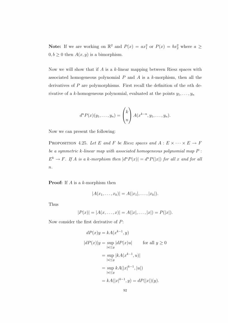
Note: If we are working on R2 and P (x) = ax21 or P (x) = bx2

2 where a ≥

0, b ≥ 0 then A(x, y) is a bimorphism.

Now we will show that if A is a k-linear mapping between Riesz spaces with

associated homogeneous polynomial P and A is a k-morphism, then all the

derivatives of P are polymorphisms. First recall the definition of the nth de-

rivative of a k-homogeneous polynomial, evaluated at the points y1, . . . , yn

dnP (x)(y1, . . . , yn) =

k

n

A(xk−n, y1, . . . , yn).

Now we can present the following:

Proposition 4.25. Let E and F be Riesz spaces and A : E × · · · × E → F

be a symmetric k-linear map with associated homogeneous polynomial map P :

Ek → F . If A is a k-morphism then |dnP (x)| = dnP (|x|) for all x and for all

n.

Proof: If A is a k-morphism then

|A(x1, . . . , xk)| = A(|x1|, . . . , |xk|).

Thus

|P (x)| = |A(x, . . . , x)| = A(|x|, . . . , |x|) = P (|x|).

Now consider the first derivative of P :

dP (x)y = kA(xk−1, y)

|dP (x)|y = sup|u|≤y

|dP (x)u| for all y ≥ 0

= sup|u|≤y

|kA(xk−1, u)|

= sup|u|≤y

kA(|x|k−1, |u|)

= kA(|x|k−1, y) = dP (|x|)(y).

92

Therefore |dP (x)| = dP (|x|).

We also need this result for a general derivative of degree n. Using the Fremlin

formula for the absolute value of a multilinear mapping makes the proof easier.

|dnP (x)|(y1, . . . , yn) = sup ∑

i1...in

|dnP (u1i1, . . . , unin

)| : um ∈ πym , 1 ≤ m ≤ n

= sup

k

n

∑i1,...,in

|A(xk−n, u1i1, . . . , unin

|.

Again since A is a k-morphism

= sup

k

n

∑i1,...,in

A(|x|k−n, |u1i1|, . . . , |unin

|)

=

k

n

A(|x|k−n, y1, . . . , yn) = dnP (|x|)(y1, . . . , yn).

Thus |dnP (x)| = dnP (|x|). Hence if A is a k-morphism |dnP (x)| = dnP (|x|)

for all x and for all n.

We will now give an example to show that the converse of the above proposition

is not true.

Example 4.26. Take P (x) = x21 + x2

2. All derivatives of P are polymorphisms

but the associated bilinear map is not a bimorphism.

We know |P (x)| = P (|x|) and the second derivative is just a constant so we

only need to consider the first derivative.

|P ′(x)| = |(2x1, 2x2)| = (|2x1|, |2x2|) = (2|x1|, 2|x2|) = P ′(|x|).

From above we know that the associated 2-linear mapping A is not a bimor-

phism.

93

We will now show that if Eand F are Riesz spaces and A : E× · · · ×E → F is

a symmetric k-linear mapping with associated homogeneous polynomial map-

ping P : Ek → F then A is a k-morphism if and only if each homogeneous

derivative of P is a polymorphism.

First we recall what the homogeneous derivative of a homogeneous polyno-

mial is. The nth homogeneous derivative of a k-homogeneous polynomial P

evaluated at a point y is defined as follows:

dnP (x)y =

k

n

A(xk−n, yn).

Now we can present the following:

Proposition 4.27. If E,F are Riesz spaces and A : Ek → F is a symmetric k-

linear mapping with associated homogeneous polynomial mapping P : Ek → F

then A is a k-morphism if and only if |dnP (x)(y)| = dnP (x)(|y|) for all x ≥ 0,

all y ∈ E and all n ≤ k.

Proof: The proof is by induction on k. We will first show the k = 3 case.

Assuming

1) |A(x2y)| = A(x2, |y|) for all x ≥ 0

2) |A(xy2)| = A(x, |y|2) for all x ≥ 0

3) |Ay3| = A(|y|3) for all y.

Polarising on x and y where x ≥ 0 and y ≥ 0 we get

|A(x, y, z)| = |14A(x+ y, x+ y, z)− 1

4A(x− y, x− y, z)|

≥∣∣|1

4A(x+ y, x+ y, z)| − |1

4A(x− y, x− y, z)|

∣∣.Using assumption 1) the first term |1

4A(x+ y, x+ y, z)| = 1

4A(x+ y, x+ y, |z|).

However we can not do the same thing with the second term as x − y is not

necessarily positive.

94

So we need a different approach. Using the Mazur-Orlicz Polarisation formula

we get

A(x, y, z) =1

2[A(x+ y, x+ y, z)− A(x, x, z)− A(y, y, z)].

So taking x ≥ 0, y ≥ 0

|A(x, y, z)| = |12[A(x+ y, x+ y, z)− A(x, x, z)− A(y, y, z)]|

≥ 1

2

∣∣|A(x+ y, x+ y, z)| − |A(x, x, z) + A(y, y, z)|∣∣

≥ 1

2[|A(x+ y, x+ y, z)| − |A(x, x, z) + A(y, y, z)|]

≥ 1

2[|A(x+ y, x+ y, z)| − |A(x, x, z)| − |A(y, y, z)|]

=1

2[A(x+ y, x+ y, |z|)− A(x, x, |z|)− A(y, y, |z|)]

= A(x, y, |z|) for all x ≥ 0, y ≥ 0.

Hence from Proposition 4.19 it follows that A is a 3-morphism.

Now assuming the result for (k − 1)-morphisms we must show it is true for

k-morphisms. In order to see this first fix x1 ≥ 0 and let

B(x2, . . . , xk) = A(x1, x2, . . . , xk).

Now assuming that |dnP (x)(y)| = dnP (x)|y| for all x ≥ 0, for all n ≤ k

|A(x, . . . , x︸ ︷︷ ︸k−n

, y, . . . , y︸ ︷︷ ︸n

)| = A(x, . . . , x︸ ︷︷ ︸k−n

, |y|, . . . , |y|︸ ︷︷ ︸n

).

Hence |B(x, . . . , x︸ ︷︷ ︸k−n−1

, y, . . . , y︸ ︷︷ ︸n

)| = B(x, . . . , x︸ ︷︷ ︸k−n−1

, |y|, . . . , |y|︸ ︷︷ ︸n

).

Thus dnQ(x)(y) = dnQ(x)|y| where Q = B, for all n ≤ k − 1.

Hence B is a (k − 1)-morphism from the induction assumption. Thus

|B(x2, . . . , xk)| = B(|x2|, . . . , |xk|)

|A(x1, x2, . . . , xk)| = A(x1, |x2|, . . . , |xk|) for all x1 ≥ 0.

95

Now from Proposition 4.19 it follows that A is a k-morphism. The converse is

trivial.

4.9. Orthosymmetric Mappings

The notion of orthosymmetric mappings was introduced by Buskes and van

Rooij [8]. We begin with the definition:

Definition 4.28. Let E and F be Archimedean Riesz spaces. A bilinear

mapping A : E ×E → F is orthosymmetric if whenever x ∧ y = 0 for x, y ∈ E

we have A(x, y) = 0.

Sometimes this definition is given in an equivalent form with |x| ∧ |y| = 0 =⇒

A(x, y) = 0. A bilinear operator B : E × E → F is symmetric if B(x, y) =

B(y, x) for all x, y ∈ E. Any orthosymmetric positive bilinear operator is

symmetric. This subtle fact was proved by Buskes and van Rooij [8].

Theorem 4.29 (Buskes and van Rooij). Let E and F be Archimedean Riesz

spaces. Then every orthosymmetric positive bilinear mapping E × E → F is

symmetric.

It is this surprising result that we want to consider. We will demonstrate that

this result is the dual of a statement about tensors. First consider the following:

x⊗s y =1

2(x⊗ y + y ⊗ x), and

x⊗a y =1

2(x⊗ y − y ⊗ x).

Thus

x⊗ y = x⊗s y + x⊗a y

96

Since we have this result for elementary tensors we can write u = us + ua for

all u ∈ E ⊗E and it is easy to verify that this decomposition is unique. Hence

we can write

E ⊗ E = (E ⊗s E)⊕ (E ⊗a E).

It follows that the Fremlin tensor product has a similar structure

E⊗E = (E⊗sE)⊕ (E⊗aE)

where the antisymmetric Fremlin tensor product of two Riesz spaces is defined

completely analogously to the symmetric Fremlin tensor product.

Let D be the subspace of E ⊗ E generated by the elementary tensors of the

form x ⊗ y where x ∧ y = 0. We shall refer to this space as the disjoint

tensor space. Then a regular bilinear form B vanishes on D if and only if B

is orthosymmetric. So with respect to the duality (E⊗E,Br(E,E)) the result

we wish to show is:

D⊥ ⊂ (E ⊗a E)⊥

and this will follow from

E ⊗a E ⊂ D.

In other words we need to show that the antisymmetric tensor product is a

subspace of the disjoint tensor space. To see this result in its simplest context

consider the following:

Example 4.30. Let D be the disjoint tensor space and E = Rk. Then

E ⊗a E ⊂ D.97

Let x = (α1, . . . , αk) ∈ Rk, y = (β1, . . . , βk) ∈ Rk. Then

x⊗a y = (α1e1 + · · ·+ αkek)⊗a (β1e1 + · · ·+ βkek)

=1

2

[(α1e1 + · · ·+ αkek)⊗ (β1e1 + · · ·+ βkek)

− (β1e1 + · · ·+ βkek)⊗ (α1e1 + · · ·+ αkek)]

=1

2

∑i,j

i6=j

(αiβj − αjβi)ei ⊗ ej.

Noting that the coefficients of ei⊗ ei = 0 for all 1 ≤ i ≤ k and that the tensors

of the form ei ⊗ ej where i 6= j, 1 ≤ i, j ≤ k are mutually disjoint we see that

E ⊗a E ⊂ D.

This example demonstrates the inclusion E ⊗a E ⊂ D in its simplest form.

We now consider C(K) spaces. Here the basis vectors e1, . . . , ek of Rk will be

replaced by a partition of unity and a delicate argument based on the proof of

theorem 1 in Buskes and van Rooij [8] will establish the result.

Theorem 4.31. Let K be a compact space and let D be the disjoint tensor

space. Then

C(K)⊗a C(K) ⊂ D

where the closure is taken with respect to the sup norm on C(K ×K).

Proof: Let h ∈ C(K) ⊗a C(K). Then h =∑

j fj ⊗a gj where fj, gj ∈ C(K).

Clearly it suffices to prove the result for an elementary antisymmetric tensor

h = f ⊗a g. Thus

h(s, t) =1

2(f(s)g(t)− g(s)f(t)).

Let ε > 0. As in [8] call a subset J of K small if

s, t ∈ J implies |f(s)− f(t)| < ε, |g(s)− g(t)| < ε.

Since K is compact we can write K =⋃N

i=1 Si where Si are small sets. Let

u1, . . . , uN ∈ C(K) be a partition of unity based on the small sets Si; then

ui ≥ 0,∑ui = 1, supp ui ⊆ Si and there exist points ti ∈ Si such that ui(ti) =

98

1, ui(tj) = 0 for i 6= j.

Set f ′ =∑f(tn)un, g′ =

∑g(tm)um. Then by a standard argument

‖f − f ′‖∞ < ε and ‖g − g′‖∞ < ε.

We claim that ‖h− f ′ ⊗a g′‖∞ < Aε where A is a constant. To see this notice

that

‖f ⊗a g − f ′ ⊗a g′‖∞ ≤ ‖(f − f ′)⊗a g‖∞ + ‖f ′ ⊗a (g − g′)‖∞

≤ ‖f − f ′‖∞‖g‖∞ + ‖f ′‖∞‖g − g′‖∞

< ε(‖g‖∞ + ‖f ′‖∞)

= Aε.

Now we need to examine f ′ ⊗a g′ more closely to show that it can almost be

written as the sum of disjoint tensors. We have

f ′ ⊗a g′ =

∑n,m

(f(sn)g(sm)− g(sn)f(sm))︸ ︷︷ ︸νnm

un ⊗ um.

For each pair of indices n,m there are two cases to consider:

Case 1: Sn ∩ Sm = ∅ implies un ∧ um = 0. In other words, un ⊗ um ∈ D.

Case 2: Sn ∩ Sm 6= ∅. In this case we get

f(sn)g(sm)− g(sn)f(sm) = (f(sn)− f(sm))g(sm) + f(sm)(g(sm)− g(sn)).

Observe that for all n,m ∈ 1, . . . , N if Sn ∩Sm 6= ∅, then |f(sn)− f(sm)| ≤ 2ε.

Hence ‖f(sn)− f(sm)‖∞ ≤ 2ε and ‖g(sn)− g(sm)‖∞ ≤ 2ε. Thus we get

f(sn)g(sm)− g(sn)f(sm) < 2εg(sm) + 2εf(sm)

< 2ε(‖g‖∞ + ‖f‖∞) = Cε

where C is a constant. Now we can write f ′ ⊗a g′ = u+ v where

u =∑n,m

un∧um=0

νnmun ⊗ um and v =∑n,m

Sn∩Sm 6=∅

νnmun ⊗ um.

99

We have

|v(s, t)| ≤∑n,m

Cεun(s)um(t)

≤ Cε∑n,m

un(s)um(t)

= Cε for all s, t, ε > 0.

Therefore ‖v‖∞ ≤ Cε. Now u =∑n,m

un∧um=0

νnmun ⊗ um belongs to D and

‖f ⊗a g − u‖∞ ≤ ‖f ⊗a g − f ′ ⊗a g′‖∞ + ‖f ′ ⊗a g

′ − u‖∞

< Aε+ ‖v‖∞

< (A+ C)ε for all ε > 0.

Therefore f ⊗a g ∈ D.

This gives a new proof of the Buskes van Rooij theorem.

Corollary 4.32. If K is a compact Hausdorff space and A : C(K)×C(K) →

R is a regular orthosymmetric bilinear mapping then A is symmetric.

Proof: Since every regular mapping is the difference of two positive mappings

it is clearly enough to prove the result for positive orthosymmetric bilinear

mappings. If A is orthosymmetric then A|D = 0. Since every positive bilinear

mapping is bounded [24] it follows that A|D = 0. Hence from the theorem we

get A = 0 on C(K)⊗a C(K). Therefore

A(f, g) = A(f ⊗ g) = A(f ⊗s g) = A(g ⊗s f) = A(g, f)

for every f, g ∈ C(K).

In order to generalise these results to Banach lattices we first need to recall

some properties of the positive projective norm for the tensor product of two

Banach lattices. We refer to [18, 44] for details.

100

The positive projective norm coincides with the projective norm on the positive

cone. Let E,F be Banach lattices. The completion of the Fremlin tensor prod-

uct of E and F with respect to the positive projective norm, E⊗|π|F is denoted

E⊗|π|F and is itself a Banach lattice. The dual of E⊗|π|F is Br(E;F ) with

the regular norm. If E,F are C(K) spaces then the positive projective norm

coincides with the injective norm, which in turn coincides with the supremum

norm. In the following proposition the closure of D is taken with respect to

the positive projective norm.

Proposition 4.33. Let E be a Banach lattice and D the disjoint tensor sub-

space of E ⊗ E. Then

E ⊗a E ⊂ D.

Proof: Take x, y ∈ E. Then x, y ∈ Eu where Eu is a principal ideal; for

example we could take u = |x| ∨ |y|. Then Eu is norm and order isomorphic to

some C(K) space. Let

DK = spanf ⊗ g : f ∧ g = 0 in C(K)⊗ C(K).

In other words DK is the disjoint tensor subspace of C(K) ⊗ C(K). Subject

to the identification of Eu with C(K) it is easy to see that DK ⊂ D. We have

shown in the theorem that x⊗a y ∈ DK . Therefore if J is the bounded linear

inclusion map

Eu ⊗|π| EuJ→ E ⊗|π| E.

We get x⊗ay = J(x⊗ay) ∈ J(DK). Since J is continuous and JDK = DK ⊂ D

we get

J(DK) ⊂ J(DK) ⊂ D.

Hence x⊗a y ∈ D.

We note that the same proof establishes the result for uniformly complete Riesz

spaces.

101

In order to define orthogonal additivity we first need to recall the following

definition:

Definition 4.34. In a Riesz space, two elements x and y are said to be disjoint

(in symbols x ⊥ y) whenever |x| ∧ |y| = 0 holds.

Now we can define orthogonal additivity.

Definition 4.35. A real valued function f on a Riesz space E is orthogonally

additive if f(x+ y) = f(x) + f(y) whenever x ⊥ y.

Sundaresan [42] introduced the class of orthogonally additive homogeneous

polynomials. To conclude we will show that a k-homogeneous polynomial

mapping on a Riesz space is orthogonally additive if and only if its associated

symmetric k-linear mapping is orthosymmetric. In order to show this we first

need to define orthosymmetric multilinear mapping and recall the definition of

an orthogonally additive function.

Let E,F be Archimedean Riesz spaces. The natural definition of an orthosym-

metric multilinear mapping A : Ek → F might be that A(x1, . . . , xk) = 0

whenever the xj are pairwise disjoint. However this does not imply that P = A

is orthogonally additive as the following example shows:

Example 4.36. Working on R2 consider the 3-linear form

A(x, y, z) = x1y1z2 + x1y2z2 + x2y1z2.

If A is orthosymmetric by the above definition then A(x, y, z) = 0 whenever

x ∧ y = y ∧ z = x ∧ z = 0. Consider the associated polynomial P = A:

P (x) = x21x2 + 2x1x

22.

Then P (e1 + e2) = 3, P (e1) = 0, P (e2) = 0 so P is not orthogonally additive.

A less obvious but ultimately more useful definition is:

102

Definition 4.37. Let E,F be Archimedean Riesz spaces. A k-linear mapping

A : Ek → F is orthosymmetric if whenever x ∧ y = 0 for x, y ∈ E we have

A(xn, yk−n) = 0 for 0 < n < k.

This definition implies the original definition considered above. To see this use

the Mazur-Orlicz polarisation formula to get:

A(x1, . . . , xk) =1

(k − 1)!

∑δi=0,1

(−1)(k−1)−∑

δiA(δ1x1 + · · ·+ δk−1xk−1)k−1xk.

Hence if x1, . . . , xk are mutually disjoint then for all δi = 0, 1 and 1 ≤ i ≤ k

we have δ1x1 + · · · + δk−1xk−1 and xk are disjoint. Hence by our definition

A(x1, . . . , xk) = 0.

Now we can state and prove our final result:

Proposition 4.38. Let P = A be a k-homogeneous polynomial on a Riesz

space E. Then P is orthogonally additive if and only if A is orthosymmetric.

Proof: First we will demonstrate the argument for the k = 2 case. Let A be

orthosymmetric and x ⊥ y. Then A(x, y) = 0. Note

P (x+ y) = A(x+ y, x+ y)

= A(x, x) + A(x, y) + A(y, x) + A(y, y)

= A(x, x) + A(y, y)

= P (x) + P (y).

Thus P is orthogonally additive.

If P is orthogonally additive then for x ⊥ y, P (x+y) = P (x)+P (y). It follows

immediately that A(x, y) = 0 and A is orthosymmetric.

For the general case consider a k-homogeneous polynomial P = A. If A is

103

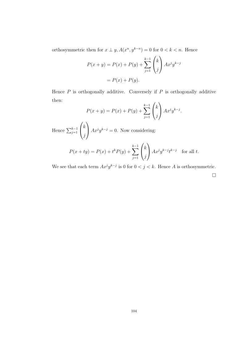
orthosymmetric then for x ⊥ y, A(xn, yk−n) = 0 for 0 < k < n. Hence

P (x+ y) = P (x) + P (y) +k−1∑j=1

kj

Axjyk−j

= P (x) + P (y).

Hence P is orthogonally additive. Conversely if P is orthogonally additive

then:

P (x+ y) = P (x) + P (y) +k−1∑j=1

kj

Axjyk−j.

Hence∑k−1

j=1

kj

Axjyk−j = 0. Now considering:

P (x+ ty) = P (x) + tkP (y) +k−1∑j=1

kj

Axjyk−jtk−j for all t.

We see that each term Axjyk−j is 0 for 0 < j < k. Hence A is orthosymmetric.

104

Bibliography

[1] C. D. Aliprantis and O. Burkinshaw, Positive Operators, Pure and Applied Mathematics,

119. Academic Press, Inc., Orlando, FL, 1985. xvi+367 pp. ISBN: 0-12-050260-7

[2] P.J. Boland and S.Dineen, Holomorphic functions on fully nuclear spaces, Bull. Soc.

Math. France 106 (1978), no. 3, 311–336

[3] G. Boole, A treatise on the calculus of finite differences, 2nd (last revised) ed. Edited by

J. F. Moulton Dover Publications, Inc., New Yourk 1960 xii+336 pp. 39.00

[4] K. Boulabiar, Some aspects of Riesz multimorphisms, Indag. Math. (N.S.) 13 (2002), no.

4, 419–432

[5] K. Boulabiar and G. Buskes, Vector lattice powers: f-algebras and functional calculus,

Comm. Algebra 34 (2006), no. 4, 1435–1442

[6] K. Boulabiar and M. A. Toumi, Lattice bimorphisms on f-algebras, Algebra Universalis

48 (2002), no. 1, 103–116

[7] G. Buskes and A. van Rooij, Bounded variation and tensor products of Banach lattices,

Positivity and its applications (Nijmegen, 2001). Positivity 7 (2003), no. 1-2, 47–59

[8] G. Buskes and A. van Rooij,Almost f-algebras: commutativity and the Cauchy-Schwarz

inequality, Positivity and its applications (Ankara, 1998). Positivity 4 (2000), no. 3, 227–

231

[9] L. Comtet, Advanced combinatorics. The art of finite and infinite expansions, Revised

and enlarged edition. D. Reidel Publishing Co., Dordrecht, 1974. xi+343 pp. ISBN: 90-

277-0441-4 05-02

[10] A. Defant and N. Kalton, Unconditionality in spaces of m-homogeneous polynomials,

Q. J. Math. 56 (2005), no. 1, 53–64

[11] S. Dineen, Complex analysis on infinite-dimensional spaces, Springer Monographs in

Mathematics. Springer-Verlag London, Ltd., London, 1999. xvi+543 pp. ISBN: 1-85233-

158-5

[12] M. Frechet, Une definition fonctionnelle de polynomes, Nouv. Ann. Math., 9, 145-162

[13] M. Frechet, Sur les fonctionnelles continues, Ann. Sc. de l’Ecole Norm. Sup. 3, 27, 1910,

193–216

[14] M. Frechet, Sur les fonctionnelles bilineaires, T.A.M.S., 16, 1915, 215–234

105

[15] M. Frechet,Les transformations ponctuelles abstraites, C.R.A. Sc., Paris, 180, 1925,

1816–1817

[16] M. Frechet, Les polynomes abstraits, Jour. Math. Pures Appl., 9, 8, 1929, 71–92

[17] D. H. Fremlin, Tensor products of Archimedean vector lattices, Amer. J. Math. 94, 1972,

777–798

[18] D. H. Fremlin, Tensor products of Banach lattices, Math. Ann. 211, 1974, 87–106

[19] B. R. Gelbaum and G. de Lamadrid, Bases of tensor products of Banach spaces, Pacific

J. Math. 11, 1961, 1281–1286

[20] J. J. Grobler and C. C. A. Labuschagne, The tensor product of Archimedean ordered

vector spaces, Math. Proc. Cambridge Philos. Soc. 104 (1988), no. 2, 331–345

[21] R. Gateaux, Sur les fonctionnelles continue et les fonctionelles analytiques, C.R.A. Sc.,

Paris, 157, 1913, 325–327

[22] R. Gateaux, Fonctions d’une infinite des variables independantes, B.S.M. Fr., 47, 1919,

70–96

[23] R. Gateaux, Sur diverses questions de calcul fonctionnel, B.S.M. Fr., 50, 1922, 1–37

[24] B. C. Grecu and R. A. Ryan, Polynomials on Banach spaces with unconditional bases,

Proc. Amer. Math. Soc. 133 (2005), no. 4, 1083–1091

[25] D. Hilbert, Wesen und Zieleiner Analysis der unendlich vielen unabhangigen Variabeln,

Rend. Circ. Mat. Palermo, 27, 1909, 59–74

[26] L. V. Kantorovic, On the moment problem for a finite interval, Dokl.Akad.Nauk SSSR

14 (1937), 531–537

[27] L. V. Kantorovic, Linear operators in semi-ordered spaces, Mat. Sb. (N. S.) 49 (1940),

209–284

[28] A. G. Kusraev, On the representation of orthosymmetric bilinear operators in vector

lattices, (Russian) Vladikavkaz. Mat. Zh. 7 (2005), no. 4, 30–34

[29] A. G. Kusraev and G. N. Shotaev, Bilinear majorizable operators, [in Russian], Studies

on Complex Analysis, Operator Theory and Mathematical Modeling (Eds. Yu. F. Ko-

robeinik and A. G. Kusraev). Vladikavkaz Scientific Center, Vladikavkaz (2004), 241-262

[30] A. G. Kusraev and S. N. Tabuev, On bilinear operators that preserve disjunction, (Rus-

sian) Vladikavkaz. Mat. Zh. 6 (2004), no. 1, 58–70

[31] M.C. Matos, On holomorphy in Banach spaces and absolute convergence of Fourier

series, Portugal. Math. 45 (1988), no. 4, 429–450 (see also Errata: ”On holomorphy in

Banach spaces and absolute covergenence of Fourier Series” Portugal. Math. 47 (1990),

no. 1, 13)

106

[32] M.C. Matos and L. Nachbin,Reinhardt domains of holomorphy in Banach spaces, Adv.

Math. 92 (1992), no. 2, 266–278

[33] S. Mazur and W. Orlicz, Grundlegende Eigenschaften der polynomischen Operationen

Erste Mitteilung, Studia Math., 5 (1934), 50–68

[34] S. Mazur and W. Orlicz, Grundlegende Eigenschaften der polynomischen Operationen,

Zweite Mitteilung, Studia Math., 5 (1934), 179–189

[35] P. Meyer-Nieberg, Banach Lattices, Universitext. Springer-Verlag, Berlin, 1991.

xvi+395 pp. ISBN: 3-540-54201-9

[36] F. Riesz, Sur la decomposition des operations lineaires, Atti Congr. Internaz. Mat.,

Bologna 1928,3 (1930), 143–148

[37] R. A. Ryan, Introduction to tensor products of Banach spaces, Springer Monographs in

Mathematics. Springer-Verlag London, Ltd., London, 2002. xiv+225 pp. ISBN: 1-85233-

437-1

[38] R. A. Ryan and B. Turett, Geometry of spaces of polynomials, J. Math. Anal. Appl.

221, no. 2, 1998, 698–711

[39] H. H. Schaefer, Banach Lattices and Positive Operators, Die Grundlehren der mathema-

tischen Wissenschaften, Band 215. Springer-Verlag, New York-Heidelberg, 1974. xi+376

pp.

[40] H. H. Schaefer, Aspects of Banach lattices, Studies in functional analysis, MAA Stud.

Math., 21, Math. Assoc. America, Washington, D.C., 1980, 158–221

[41] A. R. Schep, Factorization of positive multilinear maps, Illinois J. Math. 28 (1984), no.

4, 579–591

[42] K. Sundaresan, Geometry of spaces of homogeneous polynomials on Banach lattices,

Applied geometry and discrete mathematics, 571–586, DIMACS Ser. Discrete Math. The-

oret. Comput. Sci., 4, Amer. Math. Soc., Providence, RI, 1991

[43] G. Wittstock, Eine Bemerkung ber Tensorprodukte von Banachverbnden, (German)

Arch. Math. (Basel) 25 (1974), 627–634

[44] G. Wittstock, Ordered normed tensor products, Foundations of quantum mechanics and

ordered linear spaces (Advanced Study Inst., Marburg, 1973), Lecture Notes in Phys.,

Vol. 29, Springer, Berlin, 1974, 67–84

107