32
| Date post: | 26-Apr-2018 |
| Category: |
Documents |
| Upload: | trinhthuan |
| View: | 213 times |
| Download: | 0 times |
PONTRYAGIN'S PRINCIPLE FOR STATE-CONSTRAINED
BOUNDARY CONTROL PROBLEMS OF SEMILINEAR PARABOLIC
EQUATIONS�
EDUARDO CASASy
Abstract. This paper deals with state-constrained optimal control problems governed by semi-linear parabolic equations. We establish a minimum principle of Pontryagin's type. To deal with thestate constraints, we introduce a penalty problem by using Ekeland's principle. The key tool for theproof is the use of a special kind of spike perturbations distributed in the domain where the controlsare de�ned. Conditions for normality of optimality conditions are given.
Key Words. Pontryagin's principle, boundary control, semilinear elliptic operators, optimalityconditions, state constraints
AMS(MOS) subject classi�cation. 49K20, 35K20
1. Introduction. In the last years, some proofs of minimum principles of Pon-tryagin's type have appeared. For long time, the optimality conditions for controlproblems governed by partial di�erential equations have been given in an integralform, assuming the convexity of the control set and the di�erentiability with respectto the control and state of all functions involved in the problem. This makes a bigdi�erence with the control theory for problems governed by ordinary di�erential equa-tions, where a Pontryagin's principle is derived without the previous assumptions. Inmy opinion, the reason of this di�erence is the di�culty of extending the methods usedfor ODE's to the in�nite dimensional systems. In particular, the classical spike per-turbations of the controls localized around a point does not work properly for PDE'sbecause they lead to some equations with Dirac measures as data, which producesnon continuous solutions. This makes di�cult to treat the state constraints, speciallythe pointwise state constraints.
A new type of spike perturbations was developed by a group of mathematiciansfrom Shanghai University; see Li [25], Li and Yao [26] and Li and Yong [27]. Theyused these perturbations to study control problems of evolution equations. The spikeperturbations were de�ned by using the representation of the state given by the cor-responding semigroup. This idea was also followed by Fattorini [17], [18], Fattoriniand Frankowska [19], Fattorini and Murphy [20], [21]. Later Yong [33] and Casas andYong [14] build a similar kind of spike perturbations for elliptic equations by usingthe representation of the solution with the aid of the Green function. Afterwards,Casas suggested a new construction of the set where the perturbations are localized;see Casas [11] and Bei Hu and Yong [22]. This construction was independent of theequation. For a di�erent viewpoint explaining the true nature of this new type ofspike perturbations, the reader is referred to Casas [12], where the boundary controlof a quasilinear equation was considered.
Bonnans and Casas [5], [6] followed a di�erent approach to derive Pontryagin'sprinciple that did not use this type of spike perturbations. However it was necessaryto assume a stability condition of the optimal cost functional with respect to smallperturbation of the feasible state set.
� This researchwas partially supported by Direcci�onGeneral de Investigaci�onCient���ca y T�ecnica(Madrid)
y Departamento de Matem�atica Aplicada y Ciencias de la Computaci�on, E.T.S.I. Industriales yde Telecomunicaci�on, Universidad de Cantabria, 39071 Santander, Spain.
1
2 EDUARDO CASAS
In this paper, we consider a boundary control problem governed by a parabolicsemilinear equation. General state constraints are included in the formulation of theproblem. The idea developed in [12] is used here. To deal with the state constraints wepenalize them. But the lack of convexity of the control set and the noncontinuity withrespect to the control of the functions involved in the control problem make di�cultto formulate a penalty problem having a solution converging to the optimal controlof the original problem. Ekeland's variational principle is the key tool to obtain thesuitable penalization.
Pontryagin's principle is often established in a nonquali�ed form, which impliesthat the cost functional does not appear in the conditions for optimality. In theabsence of equality state constraints, we give a condition that leads to a quali�edoptimality system. This condition was introduced by Bonnans [4] and Bonnans andCasas [6]. It consists in assuming a certain kind of Lipschitz dependence of theoptimal cost functional with respect to small perturbations of the state constraint.It is proved that this condition is satis�ed \almost everywhere". We will distinguishstrong and weak Pontryagin's principles, depending on whether the optimality systemis quali�ed or not. To prove the strong principle we make an exact penalization ofthe state contraints.
One of the di�culties found in the optimality system is the adjoint state equation.This equation can have measures as data in the domain, on the boundary and as a �nalcondition. There are not many papers written about parabolic equations involvingmeasures. For these equations the reader is referred to Barbu and Precupanu [1],Lasiecka [24], Tr�oltzsch [32], Boccardo and Gallou�et [3], the last one dealing withquasilinear equations. Here we use the transposition method to derive a generalresult of existence and \uniqueness" of solution. Since we do not assume continuityof the coe�cients of the state equation, we need to precise in which sense the solutionis unique; see Serrin [30] for a nonuniqueness result in W 1;p
0 () (p < 2) of an ellipticproblem well posed in H1().
The paper is organized as follows. In the next section, the control problem isformulated. The state constraints are presented in an abstract framework. We showthrough some examples how the usual state constraints are included in the abstractformulation. The weak and strong Pontryagin's principles are formulated in x3 andx4 respectively. In x5, the state equation is studied and the spike perturbations arede�ned. The linear parabolic equations involving measures are analyzed in x6. All thementioned papers dealing with control of evolution equations, except [22], followedthe semigroup approach to analyze the state and adjoint state equations. Here we willfollow the variational approach, which allows to obtain some pointwise information ofthe solutions of the PDEs. This information is very important to study the controlproblems with pointwise state constraints. Finally, the proofs of weak and strongprinciples are given in x7.
2. Setting of the control problem. Let � Rn, n � 1, be an open and
bounded set, with Lipschitz boundary �. Given 0 < T < +1, we set T = � (0; T )and �T = � � (0; T ). Let (K; d) be a metric space and let us consider a functionf : �T �R� K �! R of class C1 with respect to the second variable and satisfyingthe following assumptions:
@f
@y(x; t; y; u) � 0 8(x; t; y; u) 2 �T �R�K;(2.1)
PONTRYAGIN'S PRINCIPLE FOR BOUNDARY CONTROL PROBLEMS 38<:
8M > 0 9CM > 0 such that 8(x; t; u) 2 �T �K and jyj �M
jf(x; t; 0; u)j+����@f@y (x; t; y; u)
���� � CM :(2.2)
The state equation is as follows
8>>>>><>>>>>:
@y
@t(x; t) +Ay(x; t) + a0(x; t; y(x; t)) = 0 in T ;
@�Ay(x; t) = f(x; t; y(x; t); u(x; t)) on �T ;
y(x; 0) = y0(x) in ;
(2.3)
where y0 2 C(�), A is the linear operator
Ay = �nXj=1
@xj
(nXi=1
[aij(x; t)@xiy(x; t)] + bj(x; t)y(x; t)
)
+
nXj=1
dj(x; t)@xjy(x; t) + c(x; t)y(x; t)
(2.4)
and
@�Ay(x; t) =
nXj=1
(nXi=1
[aij(x; t)@xiy(x; t)] + bj(x; t)y(x; t)
)�j(x);(2.5)
�(x) being the outward unit normal vector to � at the point x; see Casas [9] or Casasand Fern�andez [13] for an interpretation of this Neumann condition in a trace sense.Function a0 : T �R�! R is a Carath�eodory function of class C1 with respect tothe second variable and satis�es the following assumptions� 9 0 2 Lp([0; T ]; Lq()) and C1 > 0 such that
a0(x; t; y)y � 0(x; t)�C1y2 8(x; t; y) 2 T �R;(2.6)
8<:
a0(�; �; 0) 2 Lp([0; T ]; Lq()) and 8M > 0 9CM > 0 such that����@a0@y (x; t; y)
���� � CM 8(x; t) 2 T ; jyj �M ;(2.7)
where q; p 2 [1;+1] and1
p+
n
2q< 1.
As usual, we assume the following hypotheses on A:8><>:
aij; bj; dj; c 2 L1(T ); 8i; j = 1; : : : ; n;nX
i:j=1
aij(x; t)�i�j � �j�j2; 8� 2 Rn; a:e: (x; t) 2 T ; with � > 0:(2.8)
Once given the sate equation, we introduce the cost functional
J(u) =
ZT
L(x; t; yu(x; t))dxdt+
Z�T
l(x; t; yu(x; t); u(x; t))d�(x)dt;
4 EDUARDO CASAS
where yu is the solution of (2.3) associated to u; � denotes the usual (n�1)-dimensionalmeasure on � induced by the parametrization (remind that � is a Lipschitz manifold);and L : T �R�! R and l : �T �R� K �! R are of class C1 with respect to thesecond variable, L being measurable with respect to the �rst one, satisfying8<
:8M > 0 9 dM 2 L1(T ) such that 8(x; t) 2 T ; jyj �M
jL(x; t; 0)j+����@L@y (x; t; y)
���� � dM (x; t);(2.9)
and 8<:
8M > 0 9 bM 2 L1(�T ) such that 8(x; t; u) 2 �T �K; jyj �M
jl(x; t; 0; u)j+���� @l@y (x; t; y; u)
���� � bM (x; t):(2.10)
The space of controls U is formed by the measurable functions u : �T �! K suchthat the mapping
(x; t) 2 �T �! (f(x; t; y; u(x; t)); l(x; t; y; u(x; t))) 2 R2
is measurable for every y 2 R. In x5 we will prove that there exists a unique solutionof (2.3) in the space Y = C(�T )\L2([0; T ];H1()) for every u 2 U , so that functionalJ : U �! R is well de�ned.
Finally we introduce the sate constraints. Let Z be a separable Banach spaceand Q � Z a closed convex subset with nonempty interior. Given two mappings ofclass C1, G : Y �! Z and F : C(�T ) �! R
l, l � 1, we formulate the optimal controlproblem as follows
(P) Minimize fJ(u) : u 2 U ; G(yu) 2 Q;F (yu) = 0g:
Let us show how the usual examples of state constraints can be handled with thisformulation.
Example 2.1. Given a continuous function g : �T �R�! R of class C1 respectto the second variable, the constraint g(x; t; yu(x; t)) � � for all (x; t) 2 �T , with � > 0being a given number, can be written in the above framework by putting Z = C(�T ),G : Y �! C(�T ), de�ned by G(y) = g(�; y(�)), and
Q = fz 2 C(�T ) : z(x; t) � � 8(x; t) 2 �Tg:
Example 2.2. Let f(xj; tj)glj=1 � �T , then we can include the equality con-straints yu(xj; tj) = �j , 1 � j � l, in the above formulation. Indeed, it is enoughto de�ne the functions Fj : C(�T ) �! R given by Fj(y) = y(xj) � �j and to takeF = (F1; : : : ; Fl)
T . Then F is of class C1.
Example 2.3. Let g : � [0; T ]�R�! Rbe a function measurable with respectto the �rst variable, continuous with respect to the second, of class C1 with respect tothe third and such that @g=@y is also continuous in the last two variables. Moreoverit is assumed that for every M > 0 there exists a function M 2 L1() such that
jg(x; t; 0)j+����@g@y (x; t; y)
���� � M (x) a:e: x 2 ; 8t 2 [0; T ] and jyj �M:
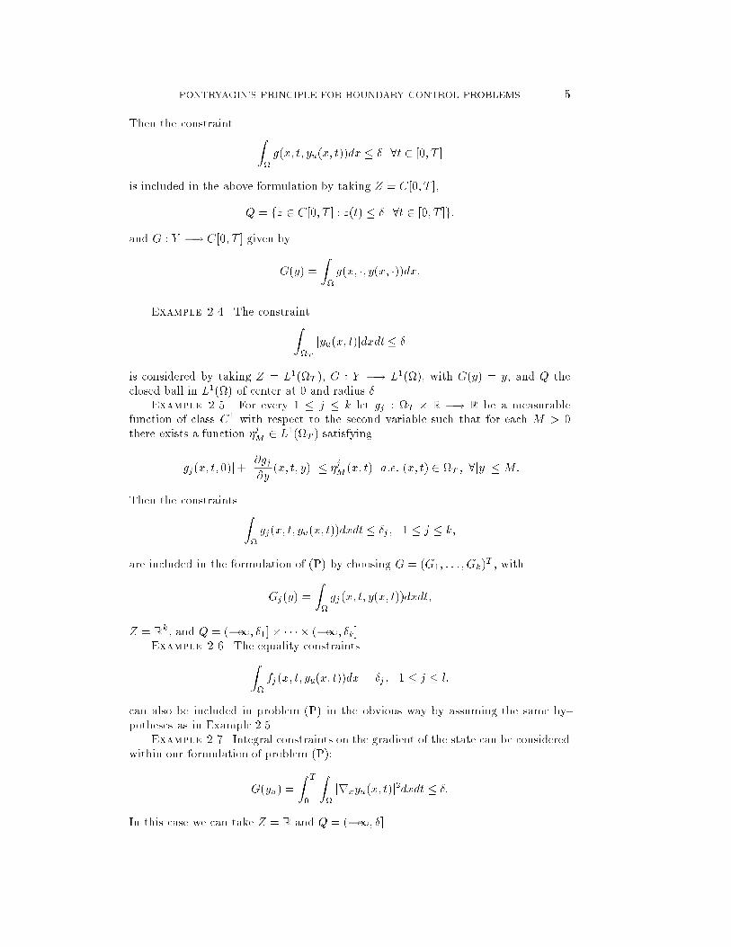
PONTRYAGIN'S PRINCIPLE FOR BOUNDARY CONTROL PROBLEMS 5
Then the constraint Z
g(x; t; yu(x; t))dx � � 8t 2 [0; T ]
is included in the above formulation by taking Z = C[0; T ],
Q = fz 2 C[0; T ] : z(t) � � 8t 2 [0; T ]g:
and G : Y �! C[0; T ] given by
G(y) =
Z
g(x; �; y(x; �))dx:
Example 2.4. The constraintZT
jyu(x; t)jdxdt� �
is considered by taking Z = L1(T ), G : Y �! L1(), with G(y) = y, and Q theclosed ball in L1() of center at 0 and radius �.
Example 2.5. For every 1 � j � k let gj : T � R �! R be a measurablefunction of class C1 with respect to the second variable such that for each M > 0there exists a function �jM 2 L1(T ) satisfying
jgj(x; t; 0)j+����@gj@y (x; t; y)
���� � �jM (x; t) a:e: (x; t) 2 T ; 8jyj �M:
Then the constraints Z
gj(x; t; yu(x; t))dxdt � �j ; 1 � j � k;
are included in the formulation of (P) by choosing G = (G1; : : : ; Gk)T , with
Gj(y) =
Z
gj(x; t; y(x; t))dxdt;
Z = Rk, and Q = (�1; �1]� � � � � (�1; �k].Example 2.6. The equality constraintsZ
fj(x; t; yu(x; t))dx = �j ; 1 � j � l;
can also be included in problem (P) in the obvious way by assuming the same hy-potheses as in Example 2.5.
Example 2.7. Integral constraints on the gradient of the state can be consideredwithin our formulation of problem (P):
G(yu) =
Z T
0
Z
jrxyu(x; t)j2dxdt � �:
In this case we can take Z = R and Q = (�1; �].
6 EDUARDO CASAS
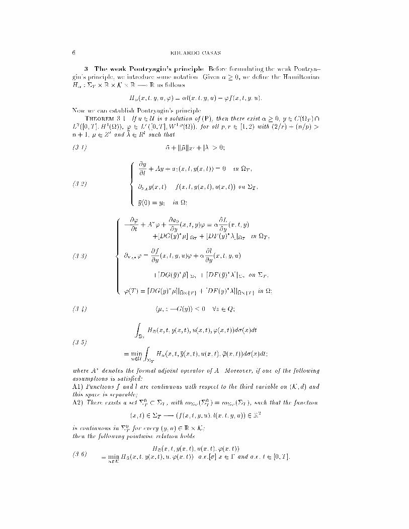
3. The weak Pontryagin's principle. Before formulating the weak Pontrya-gin's principle, we introduce some notation. Given � � 0, we de�ne the HamiltonianH� : �T �R�K �R�! R as follows
H�(x; t; y; u; ') = �l(x; t; y; u) + 'f(x; t; y; u):
Now we can establish Pontryagin's principleTheorem 3.1. If �u 2 U is a solution of (P), then there exist �� � 0, �y 2 C(�T )\
L2([0; T ];H1()), �' 2 Lr([0; T ];W 1;p()), for all p; r 2 [1; 2) with (2=r) + (n=p) >n+ 1, �� 2 Z0 and �� 2 Rl such that
��+ k��kZ0 + j��j > 0;(3.1)
8>>>>><>>>>>:
@�y
@t+A�y + a0(x; t; �y(x; t)) = 0 in T ;
@�A �y(x; t) = f(x; t; �y(x; t); �u(x; t)) on �T ;
�y(0) = y0 in ;
(3.2)
8>>>>>>>>>>>>><>>>>>>>>>>>>>:
�@ �'@t
+A� �'+@a0
@y(x; t; �y) �' = ��
@L
@y(x; t; �y)
+[DG(�y)���]jT+ [DF (�y)���]jT
in T ;
@�A� �' =@f
@y(x; t; �y; �u) �' + ��
@l
@y(x; t; �y; �u)
+[DG(�y)���]j�T+ [DF (�y)���]j�T
on �T ;
�'(T ) = [DG(�y)���]j��fTg + [DF (�y)���]j��fTg in �;
(3.3)
h��; z � G(�y)i � 0 8z 2 Q;(3.4)
Z�T
H��(x; t; �y(x; t); �u(x; t); �'(x; t))d�(x)dt
= minu2U
Z�T
H��(x; t; �y(x; t); u(x; t); �'(x; t))d�(x)dt;
(3.5)
where A� denotes the formal adjoint operator of A. Moreover, if one of the following
assumptions is satis�ed:
A1) Functions f and l are continuous with respect to the third variable on (K; d) andthis space is separable;
A2) There exists a set �0T � �T , with m�T
(�0T ) = m�T
(�T ), such that the function
(x; t) 2 �T �! (f(x; t; y; u); l(x; t; y; u)) 2 R2
is continuous in �0T for every (y; u) 2 R�K;
then the following pointwise relation holds
H��(x; t; �y(x; t); �u(x; t); �'(x; t))= minu2K
H��(x; t; �y(x; t); u; �'(x; t)) a:e:[�] x 2 � and a:e: t 2 [0; T ]:(3.6)
PONTRYAGIN'S PRINCIPLE FOR BOUNDARY CONTROL PROBLEMS 7
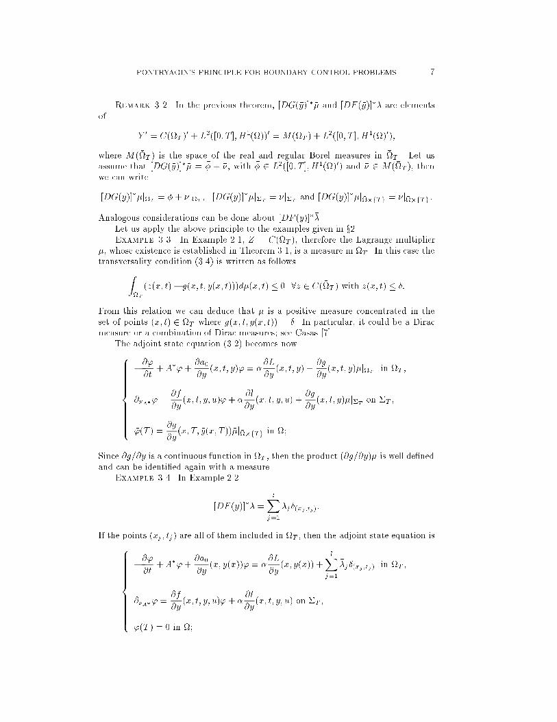
Remark 3.2. In the previous theorem, [DG(�y)]��� and [DF (�y)]��� are elementsof
Y 0 = C(�T )0 + L2([0; T ];H1())0 =M (�T ) + L2([0; T ];H1()0);
where M (�T ) is the space of the real and regular Borel measures in �T . Let usassume that [DG(�y)]��� = �� + ��, with �� 2 L2([0; T ];H1()0) and �� 2 M (�T ), thenwe can write
[DG(�y)]���jT= ��+ ��jT
; [DG(�y)]���j�T= ��j�T
and [DG(�y)]���j��fTg = ��j��fTg:
Analogous considerations can be done about [DF (�y)]���.Let us apply the above principle to the examples given in x2.Example 3.3. In Example 2.1, Z = C(�T ), therefore the Lagrange multiplier
��, whose existence is established in Theorem 3.1, is a measure in �T . In this case thetransversality condition (3.4) is written as followsZ
�T
(z(x; t)� g(x; t; �y(x; t)))d��(x; t) � 0 8z 2 C(�T ) with z(x; t) � �:
From this relation we can deduce that �� is a positive measure concentrated in theset of points (x; t) 2 �T where g(x; t; �y(x; t)) = �. In particular, it could be a Diracmeasure or a combination of Dirac measures; see Casas [7].
The adjoint state equation (3.2) becomes now8>>>>>>>>><>>>>>>>>>:
�@ �'@t
+ A� �' +@a0
@y(x; t; �y) �' = ��
@L
@y(x; t; �y) +
@g
@y(x; t; �y)��jT
in T ;
@�A� �' =@f
@y(x; t; �y; �u) �'+ ��
@l
@y(x; t; �y; �u) +
@g
@y(x; t; �y)��j�T
on �T ;
�'(T ) =@g
@y(x; T; �y(x; T ))��j��fTg in �;
Since @g=@y is a continuous function in �T , then the product (@g=@y)�� is well de�ned
and can be identi�ed again with a measure.Example 3.4. In Example 2.2
[DF (�y)]��� =
lXj=1
��j�(xj ;tj):
If the points (xj; tj) are all of them included in T , then the adjoint state equation is8>>>>>>>>><>>>>>>>>>:
�@ �'@t
+A� �'+@a0
@y(x; �y(x)) �' = ��
@L
@y(x; �y(x)) +
lXj=1
��j�(xj ;tj) in T ;
@�A� �' =@f
@y(x; t; �y; �u) �' + ��
@l
@y(x; t; �y; �u) on �T ;
�'(T ) = 0 in ;
8 EDUARDO CASAS
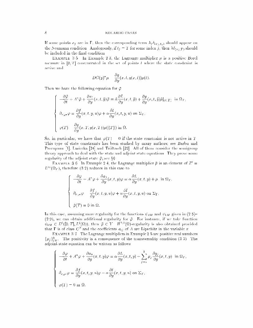
If some points xj are in �, then the corresponding term ��j�(xj ;tj) should appear on
the Neumann condition. Analogously, if tj = T for some index j, then ���(xj ;T ) shouldbe included in the �nal condition.
Example 3.5. In Example 2.3, the Lagrange multiplier �� is a positive Borelmeasure in [0; T ] concentrated in the set of points t where the state constraint isactive and
DG(�y)��� =@g
@y(x; t; �y(x; t))��(t):
Then we have the following equation for �'8>>>>>>>>><>>>>>>>>>:
�@ �'@t
+A� �' +@a0
@y(x; t; �y) �' = ��
@L
@y(x; t; �y) +
@g
@y(x; t; �y)��j(0;T ) in T ;
@�A� �' =@f
@y(x; t; �y; �u) �'+ ��
@l
@y(x; t; �y; �u) on �T ;
�'(T ) =@g
@y(x; T; �y(x; T ))��(fTg) in :
So, in particular, we have that �'(T ) = 0 if the state constraint is not active in T .This type of state constraints has been studied by many authors; see Barbu andPrecupanu [1], Lasiecka [24] and Tr�oltzsch [32]. All of them consider the semigrouptheory approach to deal with the state and adjoint state equations. They prove someregularity of the adjoint state �'; see x6.
Example 3.6. In Example 2.4, the Lagrange multiplier �� is an element of Z 0 =L1(T ), therefore (3.2) reduces in this case to8>>>>>>><
>>>>>>>:
�@ �'@t
+A� �' +@a0
@y(x; t; �y) �' = ��
@L
@y(x; t; �y) + �� in T ;
@�A� �' =@f
@y(x; t; �y; �u) �'+ ��
@l
@y(x; t; �y; �u) on �T ;
�'(T ) = 0 in :
In this case, assuming more regularity for the functions dM and bM given in (2.8){(2.9), we can obtain additional regularity for �'. For instance, if we take function bM 2 Lp([0; T ]; Lq()), then �' 2 Y . H2;1()-regularity is also obtained providedthat � is of class C2 and the coe�cients aij of A are Lipschitz in the variable x.
Example 3.7. The Lagrange multipliers in Example 2.5 are positive real numbersf��jgkj=1. The positivity is a consequence of the transversality condition (3.3). Theadjoint state equation can be written as follows8>>>>>>>>><
>>>>>>>>>:
�@ �'@t
+A� �' +@a0
@y(x; t; �y) �' = ��
@L
@y(x; t; �y) +
kXj=1
��j@gj
@y(x; t; �y) in T ;
@�A� �' =@f
@y(x; t; �y; �u) �'+ ��
@l
@y(x; t; �y; �u) on �T ;
�'(T ) = 0 in :
PONTRYAGIN'S PRINCIPLE FOR BOUNDARY CONTROL PROBLEMS 9
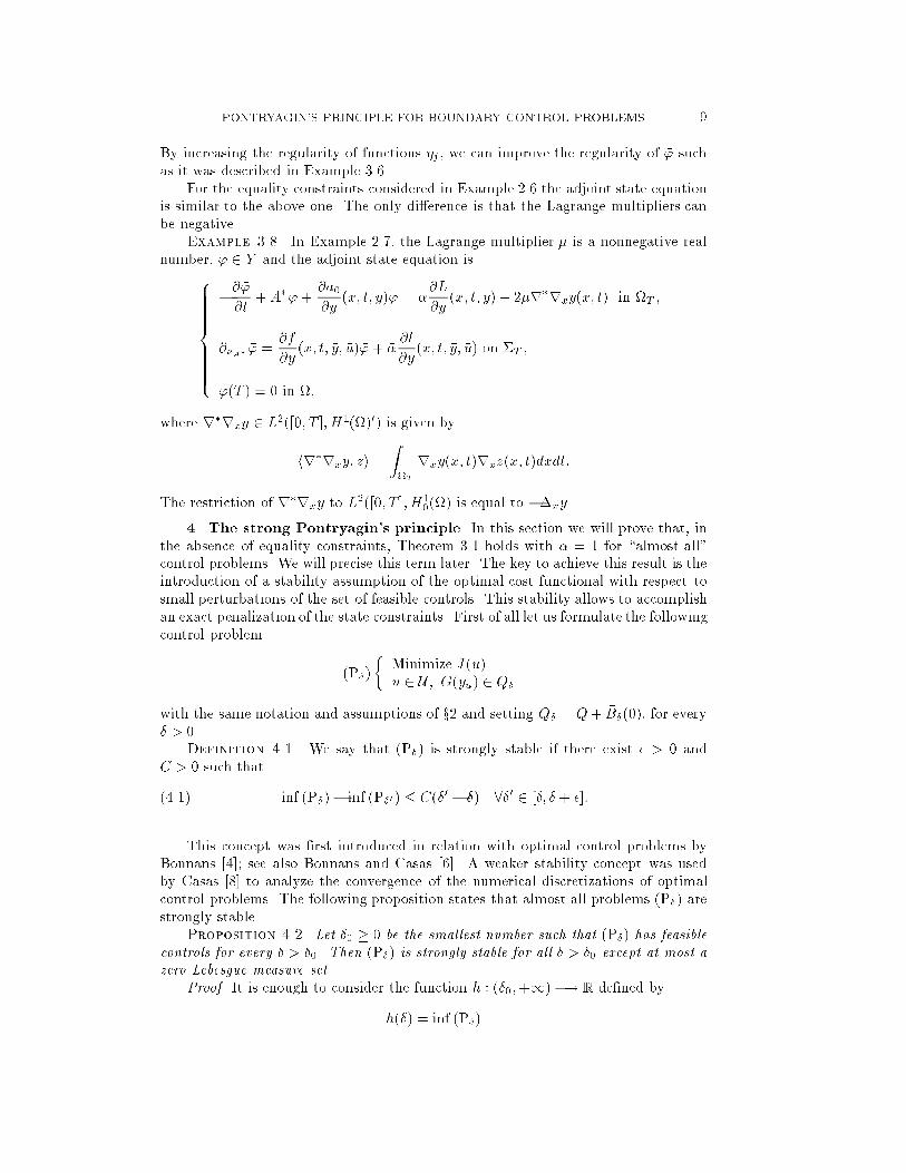
By increasing the regularity of functions �j, we can improve the regularity of �' suchas it was described in Example 3.6.
For the equality constraints considered in Example 2.6 the adjoint state equationis similar to the above one. The only di�erence is that the Lagrange multipliers canbe negative.
Example 3.8. In Example 2.7, the Lagrange multiplier �� is a nonnegative realnumber, �' 2 Y and the adjoint state equation is8>>>>>>><
>>>>>>>:
�@ �'@t
+A� �'+@a0
@y(x; t; �y) �' = ��
@L
@y(x; t; �y) + 2��r�rxy(x; t) in T ;
@�A� �' =@f
@y(x; t; �y; �u) �' + ��
@l
@y(x; t; �y; �u) on �T ;
�'(T ) = 0 in ;
where r�rxy 2 L2([0; T ];H1()0) is given by
hr�rxy; zi =ZT
rxy(x; t)rxz(x; t)dxdt:
The restriction of r�rxy to L2([0; T ];H1
0() is equal to ��xy.
4. The strong Pontryagin's principle. In this section we will prove that, inthe absence of equality constraints, Theorem 3.1 holds with �� = 1 for \almost all"control problems. We will precise this term later. The key to achieve this result is theintroduction of a stability assumption of the optimal cost functional with respect tosmall perturbations of the set of feasible controls. This stability allows to accomplishan exact penalization of the state constraints. First of all let us formulate the followingcontrol problem
(P�)
�Minimize J(u)u 2 U ; G(yu) 2 Q�
with the same notation and assumptions of x2 and setting Q� = Q+ �B�(0), for every� > 0.
Definition 4.1. We say that (P�) is strongly stable if there exist � > 0 and
C > 0 such that
inf (P�)� inf (P�0 ) � C(�0 � �) 8�0 2 [�; � + �]:(4.1)
This concept was �rst introduced in relation with optimal control problems byBonnans [4]; see also Bonnans and Casas [6]. A weaker stability concept was usedby Casas [8] to analyze the convergence of the numerical discretizations of optimalcontrol problems. The following proposition states that almost all problems (P�) arestrongly stable.
Proposition 4.2. Let �0 � 0 be the smallest number such that (P�) has feasible
controls for every � > �0. Then (P�) is strongly stable for all � > �0 except at most a
zero Lebesgue measure set.
Proof. It is enough to consider the function h : (�0;+1) �! R de�ned by
h(�) = inf (P�)
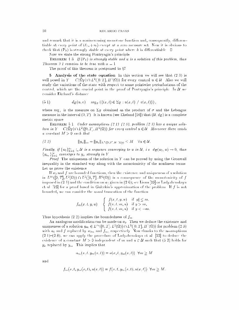
10 EDUARDO CASAS
and remark that it is a nonincreasing monotone function and, consequently, di�eren-tiable at every point of (�0;+1) except at a zero measure set. Now it is obvious tocheck that (P�) is strongly stable at every point where h is di�erentiable.
Now we state the strong Pontryagin's principle.Theorem 4.3. If (P�) is strongly stable and �u is a solution of this problem, then
Theorem 3.1 remains to be true with �� = 1.The proof of this theorem is postponed to x7.5. Analysis of the state equation. In this section we will see that (2.3) is
well posed in Y = C(�T ) \ L2([0; T ];H1()) for every control u 2 U . Also we willstudy the variations of the state with respect to some pointwise perturbations of thecontrol, which are the crucial point in the proof of Pontryagin's principle. In U weconsider Ekeland's distance
dE(u; v) = m�T(f(x; t) 2 �T : u(x; t) 6= v(x; t)g) ;(5.1)
where m�Tis the measure on �T obtained as the product of � and the Lebesgue
measure in the interval (0; T ). It is known (see Ekeland [16]) that (U ; dE) is a completemetric space.
Theorem 5.1. Under assumptions (2.1){(2.8), problem (2.3) has a unique solu-
tion in Y = C(�T )\L2([0; T ];H1()) for every control u 2 U . Moreover there exists
a constant M > 0 such that
kyuk1 + kyukL2([0;T ];H1()) �M 8u 2 U :(5.2)
Finally, if fukg1k=1 � U is a sequence converging to u in U , i.e. dE(uk; u)! 0, thenfyukg1k=1 converges to yu strongly in Y .
Proof. The uniqueness of the solution in Y can be proved by using the Gronwallinequality in the standard way along with the monotonicity of the nonlinear terms.Let us prove the existence.
If a0 and f are bounded functions, then the existence and uniqueness of a solutionin L1([0; T ]; L2()) \ L2([0; T ];H1()) is a consequence of the monotonicity of fimposed in (2.1) and the condition on a0 given in (2.6); see Lions [29] or Ladyzhenskayaet al. [23] for a proof based in Galerkin's approximation of the problem. If f is notbounded, we can consider the usual truncation of the function
fm(x; t; y; u) =
8<:
f(x; t; y; u) if jyj � m;
f(x; t;m; u) if y > m;
f(x; t;m; u) if y < �m:Thus hypothesis (2.2) implies the boundedness of fm.
An analogous modi�cation can be made on a0. Then we deduce the existence anduniqueness of a solution ym 2 L1([0; T ]; L2())\L2([0; T ];H1()) for problem (2.3)with a0 and f replaced by a0m and fm, respectively. Now thanks to the assumptions(2.1){(2.8), we can apply the procedure of Ladyzhenskaya et al. [23] to deduce theexistence of a constant M > 0 independent of m and u 2 U such that (5.2) holds foryu replaced by ym. This implies that
am(x; t; ym(x; t)) = a(x; t; ym(x; t)) 8m �M
and
fm(x; t; ym(x; t); u(x; t)) = f(x; t; ym(x; t); u(x; t)) 8m �M:

PONTRYAGIN'S PRINCIPLE FOR BOUNDARY CONTROL PROBLEMS 11
Consequently, the uniqueness of a solution of (2.3) lets to obtain the identity ym = yuand the inequality (5.2).
In order to prove the continuity of yu, we �rst suppose that y0 2 C�(�T ) forsome constant � 2 (0; 1]. Then, by applying the results of Di Benedetto [2], wededuce that yu 2 C�;�=2(�T ) for some � 2 (0; �]. When y0 is not a H�older function,we can take a sequence fy0kg1k=1 � C�(�T ) converging uniformly to y0 in �T . Thenthe corresponding solutions of (2.3), denoted by yk, are H�older functions. Now, byapplying the methods of [23] is easy to deduce the convergence yk ! yu in L1(T ),which proves the continuity of yu.
Finally, the convergence yuk ! yu in L2([0; T ];H1()) when dE(uk; u) ! 0 iseasily derived. The uniform convergence is obtained again by using the arguments of[23].
The rest of the section is devoted to the proof of the following theoremTheorem 5.2. Let u; v 2 U . Given � 2 (0; 1), there exist m�T
-measurable sets
E� � �T , with m�T(E�) = �m�T
(�T ), such that if we de�ne
u�(x; t) =
�u(x; t) if (x; t) 2 �T nE�v(x; t) if (x; t) 2 E�;
and if we denote by y� and y the states corresponding to u� and u, respectively, then
the following equalities hold
y� = y + �z + r�; lim�!0
1
�kr�kY = 0;(5.3)
and
J(u�) = J(u) + �z0 + r0�; lim�!0
1
�r0� = 0;(5.4)
where z 2 Y satis�es8>>>>>>>>>>><>>>>>>>>>>>:
@z
@t+ Az +
@a0
@y(x; t; y(x; t))z = 0 in T
@�Az =@f
@y(x; t; y(x; t); u(x; t))z
+f(x; t; y(x; t); v(x; t))� f(x; t; y(x; t); u(x; t)) on �T ;
z(x; 0) = 0 in
(5.5)
and
z0 =
ZT
@L
@y(x; t; y(x; t))z(x; t)dxdt+
Z�T
@l
@y(x; t; y(x; t); u(x; t))z(x; t)d�(x)dt
+
Z�T
[l(x; t; y(x; t); v(x; t))� l(x; t; y(x; t); u(x; t))]d�(x)dt:(5.6)
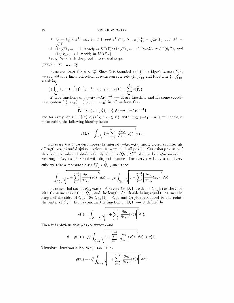
The �rst step is the proof of the following resultProposition 5.3. For every 0 < � < 1 there exists a sequence of m�T
-
measurable sets fEkg1k=1, satisfying
12 EDUARDO CASAS
1. Ek = Ek� � Jk, with Ek � � and Jk � (0; T ), �(Ek�) =p��(�) and jJkj =p
�T .
2. (1=p�)�Ek
�
! 1 �weakly in L1(�); (1=p�)�Jk ! 1 �weakly in L1(0; T ); and
(1=�)�Ek! 1 �weakly in L1(�T ).
Proof. We divide the proof into several steps.
STEP 1. The sets Ek�.
Let us construct the sets Ek�. Since is bounded and � is a Lipschitz manifold,we can obtain a �nite collection of �-measurable sets f�rgdr=1 and functions fargdr=1satisfying
(i)
d[r=1
�r = �,o
�iT o
�j= ; if i 6= j and �(�) =
dXr=1
�(o
�r).
(ii) The functions ar : (���;+��)n�1 �! R are Lipschitz and for some coordi-
nate system (x0r; xr;n) = (xr;1; : : : ; xr;n) in Rn we have that
o
�r= f(x0r; ar(x0r)) : x0r 2 (���;+��)n�1g
and for every set E = f(x0r; ar(x0r)) : x0r 2 Fg, with F � (���;+��)n�1 Lebesgue
measurable, the following identity holds
�(E) =
ZF
vuut1 +
n�1Xi=1
���� @ar@xr;i(x0r)
����2
dx0r:
For every k 2 N we decompose the interval [���;+��] into k closed subintervalsof length 2��=k and disjoint interiors. Now we made all possible Cartesian products of
these subintervals and obtain a family of cubes fQk;igkn�1i=1 of equal Lebesgue measure,covering [���;+��]
n�1 and with disjoint interiors. For every r = 1; : : : ; d and every
cube we take a measurable set F rk;j �o
Qk;j such that
ZFrk;j
vuut1 +
n�1Xi=1
���� @ar@xr;i(x0r)
����2
dx0r =p�
ZQk;j
vuut1 +
n�1Xi=1
���� @ar@xr;i(x0r)
����2
dx0r:
Let us see that such a F rk;j exists. For every t 2 [0; 1] we de�ne Qk;j(t) as the cubewith the same center than Qk;j and the length of each side being equal to t times thelength of the sides of Qk;j. So Qk;j(1) = Qk;j and Qk;j(0) is reduced to one point:the center of Qk;j. Let us consider the function g : [0; 1] �! R de�ned by
g(t) =
ZQk;j(t)
vuut1 +
n�1Xi=1
���� @ar@xr;i(x0r)
����2
dx0r:
Then it is obvious that g is continuous and
0 = g(0) <p�
ZQk;j
vuut1 +
n�1Xi=1
���� @ar@xr;i(x0r)
����2
dx0r < g(1):
Therefore there exists 0 < t0 < 1 such that
g(t0) =p�
ZQk;j
vuut1 +
n�1Xi=1
���� @ar@xr;i(x0r)
����2
dx0r:
PONTRYAGIN'S PRINCIPLE FOR BOUNDARY CONTROL PROBLEMS 13
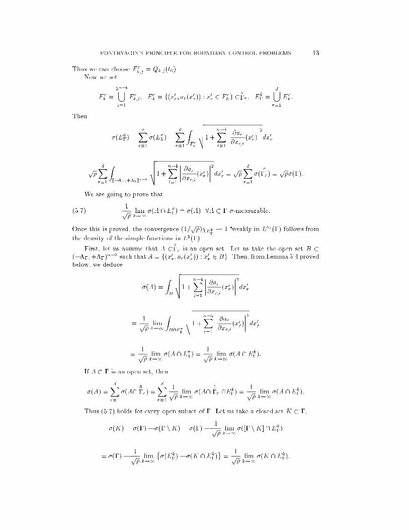
Thus we can choose F rk;j = Qk;j(t0).Now we set
F rk =
kn�1[i=1
F rk;i; Erk = f(x0r; ar(x0r)) : x0r 2 F rkg �o
�r; Ek� =
d[r=1
Erk:
Then
�(Ek�) =
dXr=1
�(Erk) =
dXr=1
ZFrk
vuut1 +
n�1Xi=1
���� @ar@xr;i(x0r)
����2
dx0r =
p�
dXr=1
Z[���;+��]n�1
vuut1 +
n�1Xi=1
���� @ar@xr;i(x0r)
����2
dx0r =p�
dXr=1
�(o
�r) =p��(�):
We are going to prove that
1p�
limk!1
�(A \Ek�) = �(A) 8A � � �-measurable:(5.7)
Once this is proved, the convergence (1=p�)�Ek
�
! 1 �weakly in L1(�) follows from
the density of the simple functions in L1(�).
First, let us assume that A � o
�r is an open set. Let us take the open set B �(���;+��)
n�1 such that A = f(x0r; ar(x0r)) : x0r 2 Bg. Then, from Lemma 5.4 provedbelow, we deduce
�(A) =
ZB
vuut1 +
n�1Xi=1
���� @ar@xr;i(x0r)
����2
dx0r
=1p�
limk!1
ZB\Fr
k
vuut1 +
n�1Xi=1
���� @ar@xr;i(x0r)
����2
dx0r
=1p�
limk!1
�(A \Erk) =1p�
limk!1
�(A \Ek�):
If A � � is an open set, then
�(A) =
dXr=1
�(A\ 0
�r) =
dXr=1
1p�
limk!1
�(A\ 0
�r \Ek�) =1p�
limk!1
�(A \Ek�):
Thus (5.7) holds for every open subset of �. Let us take a closed set K � �,
�(K) = �(�) � �(� nK) = �(�) � 1p�
limk!1
�([� nK] \Ek�)
= �(�) � 1p�
limk!1
��(Ek�)� �(K \Ek�)
=
1p�
limk!1
�(K \Ek�):
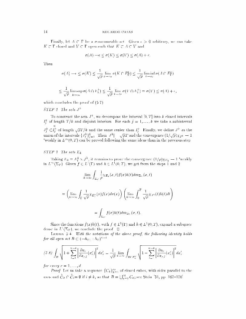
14 EDUARDO CASAS
Finally, let A � � be a �-measurable set. Given � > 0 arbitrary, we can takeK � � closed and V � � open such that K � A � V and
�(A) � � � �(K) � �(V ) � �(A) + �:
Then
�(A) � � � �(K) � 1p�
limk!1
�(K \Ek�) �1p�lim infk!1
�(A \Ek�)
� 1p�lim supk!1
�(A \Ek�) �1p�
limk!1
�(V \Ek�) = �(V ) � �(A) + �;
which concludes the proof of (5.7).
STEP 2. The sets Jk.
To construct the sets Jk, we decompose the interval [0; T ] into k closed intervalsIkj of length T=k and disjoint interiors. For each j = 1; : : : ; k we take a subinterval
Jkj �0
Ikj of lengthp�T=k and the same center than Ikj . Finally, we de�ne J
k as the
union of the intervals fJkj gkj=1. Then jJkj =p�T and the convergence (1=
p�)�Jk ! 1
�weakly in L1(0; T ) can be proved following the same ideas than in the previous step.
STEP 3. The sets Ek.
Taking Ek = Ek��Jk, it remains to prove the convergence (1=�)�Ek! 1 �weakly
in L1(�T ). Given f 2 L1(�) and h 2 L1(0; T ), we get from the steps 1 and 2
limk!1
Z�T
1
��Ek
(x; t)f(x)h(t)dm�T(x; t)
=
�limk!1
Z�
1p��Ek
�
(x)f(x)d�(x)
� limk!1
Z T
0
1p��Jk (t)h(t)dt
!
=
Z�T
f(x)h(t)dm�T(x; t):
Since the functions f(x)h(t), with f 2 L1(�) and h 2 L1(0; T ), expand a subspacedense in L1(�T ), we conclude the proof.
Lemma 5.4. With the notations of the above proof, the following identity holds
for all open set B � (���;+��)n�1
ZB
vuut1 +
n�1Xi=1
���� @ar@xr;i(x0r)
����2
dx0r =1p�
limk!1
ZB\Fr
k
vuut1 +
n�1Xi=1
���� @ar@xr;i(x0r)
����2
dx0r(5.8)
for every r = 1; : : : ; d.Proof. Let us take a sequence fCkg1k=1 of closed cubes, with sides parallel to the
axes ando
Ck \o
Ci= ; if i 6= k, so that B =S1k=1Ck; see Stein [31, pp. 167{170].
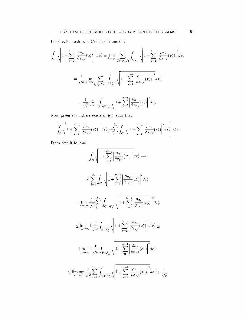
PONTRYAGIN'S PRINCIPLE FOR BOUNDARY CONTROL PROBLEMS 15
Fixed r, for each cube Cl it is obvious that
ZCl
vuut1 +
n�1Xi=1
���� @ar@xr;i(x0r)
����2
dx0r = limk!1
XQk;j�Cl
ZQk;j
vuut1 +
n�1Xi=1
���� @ar@xr;i(x0r)
����2
dx0r
=1p�
limk!1
XQk;r�Cl
ZFrk;j
vuut1 +
n�1Xi=1
���� @ar@xr;i(x0r)
����2
dx0r
=1p�
limk!1
ZCl\F
rk
vuut1 +
n�1Xi=1
���� @ar@xr;i(x0r)
����2
dx0r:
Now, given � > 0 there exists k� 2 N such that������ZB
vuut1 +
n�1Xi=1
���� @ar@xr;i(x0r)
����2
dx0r �k�Xl=1
ZCl
vuut1 +
n�1Xi=1
���� @ar@xr;i(x0r)
����2
dx0r
������ < �:
From here it follows
ZB
vuut1 +
n�1Xi=1
���� @ar@xr;i(x0r)
����2
dx0r � �
�k�Xl=1
ZCl
vuut1 +
n�1Xi=1
���� @ar@xr;i(x0r)
����2
dx0r
= limk!1
1p�
k�Xl=1
ZCl\F
rk
vuut1 +
n�1Xi=1
���� @ar@xr;i(x0r)
����2
dx0r
� lim infk!1
1p�
ZB\Fr
k
vuut1 +
n�1Xi=1
���� @ar@xr;i(x0r)
����2
dx0r �
lim supk!1
1p�
ZB\Fr
k
vuut1 +
n�1Xi=1
���� @ar@xr;i(x0r)
����2
dx0r
� lim supk!1
1p�
k�Xl=1
ZCl\F
rk
vuut1 +
n�1Xi=1
���� @ar@xr;i(x0r)
����2
dx0r +�p�
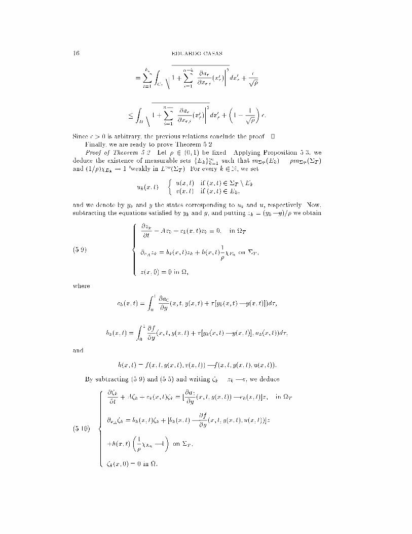
16 EDUARDO CASAS
=
k�Xl=1
ZCl
vuut1 +
n�1Xi=1
���� @ar@xr;i(x0r)
����2
dx0r +�p�
�ZB
vuut1 +
n�1Xi=1
���� @ar@xr;i(x0r)
����2
dx0r +
�1 +
1p�
��:
Since � > 0 is arbitrary, the previous relations conclude the proof.Finally, we are ready to prove Theorem 5.2.Proof of Theorem 5.2. Let � 2 (0; 1) be �xed. Applying Proposition 5.3, we
deduce the existence of measurable sets fEkg1k=1 such that m�T(Ek) = �m�T
(�T )and (1=�)�Ek
! 1 �weakly in L1(�T ). For every k 2 N, we set
uk(x; t) =
�u(x; t) if (x; t) 2 �T nEkv(x; t) if (x; t) 2 Ek;
and we denote by yk and y the states corresponding to uk and u, respectively. Now,subtracting the equations satis�ed by yk and y, and putting zk = (yk�y)=� we obtain8>>>>>>><
>>>>>>>:
@zk
@t+Azk + ck(x; t)zk = 0; in T
@�Azk = bk(x; t)zk + h(x; t)1
��Ek
on �T ;
z(x; 0) = 0 in ;
(5.9)
where
ck(x; t) =
Z 1
0
@a0
@y(x; t; y(x; t) + � [yk(x; t)� y(x; t)])d�;
bk(x; t) =
Z 1
0
@f
@y(x; t; y(x; t) + � [yk(x; t)� y(x; t)]; uk(x; t))d�;
and
h(x; t) = f(x; t; y(x; t); v(x; t))� f(x; t; y(x; t); u(x; t)):
By subtracting (5.9) and (5.5) and writing �k = zk � z, we deduce8>>>>>>>>>>>>><>>>>>>>>>>>>>:
@�k
@t+ A�k + ck(x; t)�k = [
@a0
@y(x; t; y(x; t))� ck(x; t)]z; in T
@�A�k = bk(x; t)�k + [bk(x; t)�@f
@y(x; t; y(x; t); u(x; t))]z
+h(x; t)
�1
��Ek
� 1
�on �T ;
�k(x; 0) = 0 in :
(5.10)
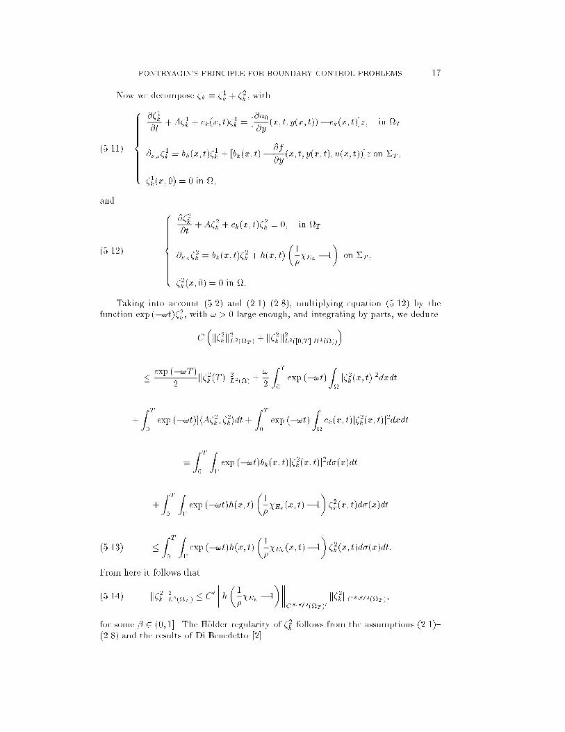
PONTRYAGIN'S PRINCIPLE FOR BOUNDARY CONTROL PROBLEMS 17
Now we decompose �k = �1k + �2k , with8>>>>>>><>>>>>>>:
@�1k@t
+A�1k + ck(x; t)�1k = [
@a0
@y(x; t; y(x; t))� ck(x; t)]z; in T
@�A�1k = bk(x; t)�
1k + [bk(x; t)� @f
@y(x; t; y(x; t); u(x; t))]z on �T ;
�1k(x; 0) = 0 in ;
(5.11)
and 8>>>>>>><>>>>>>>:
@�2k@t
+A�2k + ck(x; t)�2k = 0; in T
@�A�2k = bk(x; t)�
2k + h(x; t)
�1
��Ek
� 1
�on �T ;
�2k(x; 0) = 0 in :
(5.12)
Taking into account (5.2) and (2.1){(2.8), multiplying equation (5.12) by thefunction exp (�!t)�2k , with ! > 0 large enough, and integrating by parts, we deduce
C�k�2kk2L2(T )
+ k�2kk2L2([0;T ];H1())
�
� exp (�!T )2
k�2k(T )k2L2() +!
2
Z T
0
exp (�!t)Z
j�2k(x; t)j2dxdt
+
Z T
0
exp (�!t)]hA�2k ; �2kidt+Z T
0
exp (�!t)Z
ck(x; t)j�2k(x; t)j2dxdt
=
Z T
0
Z�
exp (�!t)bk(x; t)j�2k(x; t)j2d�(x)dt
+
Z T
0
Z�
exp (�!t)h(x; t)�1
��Ek
(x; t)� 1
��2k(x; t)d�(x)dt
�Z T
0
Z�
exp (�!t)h(x; t)�1
��Ek
(x; t)� 1
��2k(x; t)d�(x)dt:(5.13)
From here it follows that
k�2kk2L2(T )� C0
h�1
��Ek
� 1
� C�;�=2(�T )0
k�2kkC�;�=2(�T );(5.14)
for some � 2 (0; 1]. The H�older regularity of �2k follows from the assumptions (2.1){(2.8) and the results of Di Benedetto [2].
18 EDUARDO CASAS
On the other hand, for � 2 (0; �), the inclusions
C�;�=2(�T ) � C�;�=2(�T ) � L2(T )
are compact. Then we can apply the Lions lemma [28] to obtain
k�2kkC�;�=2(�T )� �k�2kkC�;�=2(�T )
+C�k�2kkL2(T ):(5.15)
Since y, yk and h are uniformly bounded, the H�older estimate of �2k can be chosendepending only on �
k�2kkC�;�=2(�T )� C� 8k 2 N:(5.16)
Taking � = �=(2[1 + C�]) in (5.15) and using (5.14) and (5.16), it follows
k�2kkC�;�=2(�T )� �
2+ C�
(C0 h�1
��Ek
� 1
� C�;�=2(�T )0
C�
)1=2
=�
2+ C0�
h�1
��Ek
� 1
� 1=2
C�;�=2(�T )0
:(5.17)
Then, for � �xed, the convergence (1=�)�Ek! 1 �weakly in L1(�T ), the bound-
edness of h and the compactness of the inclusion L1(�T ) � C�;�=2(�T )0 implies the
the strong convergence (1=�)h�Ek! h in C�;�=2(�T )
0. Therefore we can take k� 2 Nlarge enough in such a way that����
Z�T
h0(x; t)
�1
��Ek
� 1
�d�(x)dt
����+ h(x; t)
�1
��Ek
� 1
� C�;�=2(�T )0
<�2
4(1 + C0�)28k � k�;(5.18)
where
h0(x; t) = l(x; t; y(x; t); v(x; t))� l(x; t; y(x; t); u(x; t)):
Let us set E� = Ek� , u� = uk� and the analogous changes for y�, ��, �i�, i = 1; 2.
It is obvious that dE(u�; u)! 0 when �! 0. Hence Theorem 5.1 implies that y� ! y
in Y . This convergences along with the estimates of Di Benedetto [2] allow to deducefrom (5.11) the strong convergence �1� ! 0 in Y when � ! 0. Combining this with(5.13), (5.17) and (5.18), it is easy to derive the strong convergence �� ! 0 in Y ,which proves (5.3).
To conclude the proof it is enough to note that
J(u�)� J(u)
�� z0
=
ZT
�L(x; t; y�(x; t))� L(x; t; y(x; t))
�� @L
@y(x; t; y(x; t))z(x; t)
�dxdt
PONTRYAGIN'S PRINCIPLE FOR BOUNDARY CONTROL PROBLEMS 19
Z�T
�l(x; t; y�(x; t); u�(x; t))� l(x; t; y(x; t); u�(x; t))
�
� @l
@y(x; t; y(x; t); u(x; t))z(x; t)
�d�(x)dt
+
Z�T
h0(x; t)
�1
��E�
(x; t)� 1
�d�(x)dt
and to take into account the convergences previously established and (5.18).
6. Linear parabolic equations involving measure data. Let � be a regularBorel measure in �T . We can write � = �T
+ ��T+ �T + �0, where �T
= �jT,
��T= �j�T
, �T = �j��fTg and �0 = �j��f0g. The aim of this section is the study ofthe following problem 8>>>>><
>>>>>:
�@'@t
+ A�' = �Tin T ;
@�A�' = ��Ton �T ;
'(T ) = �T in �:
(6.1)
The reader is referred to Boccardo and Gallou�et [3] for the study of a quasilinearparabolic equation with a measure in T as datum. Here we improve the results of[3] by exploiting the linearity of the equation.
Let us denote
Y0 = fy 2 Y : y(x; 0) = 0 8x 2 g:
Definition 6.1. Given p; r 2 [1; 2), with (2=r) + (n=p) > n+ 1, we will say that
a function ' 2 Lr([0; T ];W 1;p()) is a solution of (6.1) if for every y 2 Y0 \C1(�T )
ZT
8<:@y
@t' +
nXj=1
"nXi=1
aij@xiy@xj'+ bjy@xj' + dj@xjy'
#+ cy'
9=; dxdt =
Z�T
yd�(x; t) =
ZT
yd�T(x; t) +
Z�T
yd��T(x; t) +
Z�
y(x; T )d�T (x):(6.2)
Let us note that (6.2) implies that �(@'=@t) +A�' = �Tin the distribution sense
in T . Let us take ~w = (w1; : : : ; wn+1), with
wi =
nXj=1
aij@xj' + di'; 1 � i � n; and wn+1 = ':
Then ~w 2 Lq(T )n+1, q = minfr; pg< (n + 1)=n, and
div(x;t) ~w =@'
@t+
nXi=1
@xi
24 nXj=1
aij@xj' + di'
35 =
@'
@t� A�'+
nXi=1
bi@xi'+ c'
20 EDUARDO CASAS
= ��T+
nXi=1
bi@xi'+ c' 2M (T ):(6.3)
Thus we have ~w 2 V q(T ),V q(T ) = f~w 2 Lq(T )n+1 : div(x;t)~w 2M (T )g:
This space, endowed with the graph norm, is a Banach space. We have the followingresult
Theorem 6.2 (Casas [10]). Given q 2 (1; (n + 1)=n), there exists a unique
continuous linear mapping �T : V q(T ) �!W�1=q;q(@T ) satisfying
�T (~w) = ~w � ~�T 8~w 2 C1(�T )(6.4)
and ZT
~w � r(x;t)�dxdt+ hdiv(x;t) ~w; �iM(T );Cb(T )
= h �T (~w); (�)iW�1=q;q (@T );W1=q;q0 (@T )8� 2W 1;q0(T );(6.5)
where Cb(T ) is the space of bounded and continuous functions in T and ~�T (x; t) isthe outward unit normal vector to @T at the point (x; t).
By applying this theorem to the function ~w de�ned above and using (6.2) and(6.3), we have for all y 2 Y0 \C1(�T )
h �T (~w); (y)iW�1=q;q (@T );W1=q;q0 (@T )=
ZT
~w � r(x;t)ydxdt+ hdiv(x;t) ~w; yiM(T );Cb(T ) =
ZT
8<:@y
@t'+
nXi=1
24 nXj=1
aij@xiy@xj'+ biy@xi'+ di@xiy'
35 + cy'
9=; dxdt
�ZT
yd�T=
Z T
0
Z�
yd��T(x; t) +
Z
y(x; T )d�T (x):
From the identity
h �T (~w); (y)iW�1=q;q (@T );W1=q;q0(@T )=
Z T
0
Z�
yd��T(x; t) +
Z
y(x; T )d�T (x)
and taking into account that
~�T (x; t) =
�~�(x)0
�8(x; t) 2 �T and ~�T (x; T ) =
�~01
�8x 2 ;
we can identify
@�A�' = �T (~!)j�T= ��T
and '(x; T ) = �T (~!)j��fTg = �T :

PONTRYAGIN'S PRINCIPLE FOR BOUNDARY CONTROL PROBLEMS 21
Now we have the following result of existence and uniqueness of solution forproblem (6.1).
Theorem 6.3. There exists a unique function ' 2 Lr([0; T ];W 1;p()), 8r; p 2[1; 2) with (2=r) + (n=p) > n+ 1, such that it is a solution of (6.1) and
ZT
�@y
@t+Ay
�'dxdt+
Z�T
@�Ay'd�(x)dt =
Z�T
yd�(x; t) 8y 2 Y 10 ;(6.6)
with
Y 10 = fy 2 Y0 : @y@t
+ Ay 2 L1(T ) and @�Ay 2 L1(�T )g:
Moreover there exists a constant Cr;p > 0 independent of � such that
k'kLr([0;T ];W1;p()) � Cr;pk�kM(�T ):(6.7)
Proof. Let ffkgk � C(�T ), fgkgk � C(� � [0; T ]) and fhkgk � C(�) such thatfk ! �T
, gk ! ��Tand hk ! �T
�weakly inM (T ),M (�T ) andM (�) respectively.Moreover we can assume that
kfkkL1(T ) � k�TkM(T ); kgkkL1(�T ) � k��T
kM(�T ) and khkkL1() � k�TkM(�):
Let us take 'k 2 Y such that
8>>>>><>>>>>:
�@'k@t
+A�'k = fk in T ;
@�A�'k = gk on �T ;
'k(T ) = hk in :
(6.8)
Now for every = ( 0; 1; : : : ; n) 2 D(T )n+1, we denote by y the solution inY of 8>>>>>>><
>>>>>>>:
@y
@t+ Ay = 0 �
nXj=1
@xj j in T ;
@�Ay = 0 on �T ;
y(0) = 0 in :
(6.9)
Then
ZT
0@ 0'k + nX
j=1
j@xj'k
1A dxdt =
ZT
�@y
@t+Ay
�'kdxdt =
ZT
��@'k@t
+ A�'k
�y dxdt+
Z�T
@�A�'ky d�(x)dt+
Z
'k(T )y (T )dx:(6.10)
22 EDUARDO CASAS
Using (6.8) and the properties of fk, gk and hk, we deduce from (6.8)
ZT
0@ 0'k + nX
j=1
j@xj'k
1A dxdt
� k�kM(�T )ky kC(�T )
� Cr;pk�kM(�T )
nXj=0
k jkLr0([0;T ];Lp0 ());(6.11)
the last inequality being a consequence of the estimates for the solution of (6.9);see Di Benedetto [2] and Ladyzhenskaya et al. [23]. From the density of the spacef 0�
Pnj=1 @xj j : 2 D(T )n+1g in Lr
0
([0; T ];W 1;p()0) and estimate (6.11) follows
the boundedness of f'kgk in the space Lr([0; T ];W 1;p()). Moreover, by taking asubsequence if necessary, we can assume that 'k ! ' weakly in Lr([0; T ];W 1;p())and (6.7) is satis�ed.
Let us prove that ' does not depend on r and p. Indeed, passing to the limit in(6.10) and remembering that y (0) = 0, we get
ZT
0@ 0'+
nXj=1
j@xj'
1A dxdt =
Z�T
y d� 8 2 D(T )n+1:(6.12)
It is obvious that there is at most one function ' in L1([0; T ];W 1;1()) satisfying(6.12), which proves that ' is independent of r and p.
Given y 2 Y0 \C1(�T ), multiplying (6.8) by y and integrating by parts, follows
ZT
8<:@y
@t'k +
nXj=1
"nXi=1
aij@xiy@xj'k + bjy@xj'k + dj@xjy'k
#+ cy'k
9=;dxdt =
ZT
fkydxdt+
Z�T
gkyd�(x)dt+
Z
hky(T )dx:
Now passing to the limit we deduce (6.2) and consequently ' is a solution of (6.1).Let us prove (6.6). Given y 2 Y10 , multiplying (6.8) by y and integrating by
parts, we deduce ZT
fkydxdt+
Z�T
gkyd�(x)dt +
Z
hky(T )dx
=
ZT
�@y
@t+ Ay
�'kdxdt+
Z�T
@�Ay'kd�(x)dt:
Now (6.6) is obtained by passing to the limit.Finally, the uniqueness of ' follows from (6.6). Indeed, the regularity results for
the Neumann problem associated to the operator (@=@t) + A (see [2] or [23]) provethe surjectivity of the mapping
y 2 Y10 �! (@y
@t+ Ay; @�Ay) 2 L1(T )� L1(�T ):
PONTRYAGIN'S PRINCIPLE FOR BOUNDARY CONTROL PROBLEMS 23
This along with (6.6) implies that the zero function of Lr([0; T ];W 1;p()) is the onlyone satisfyingZ
T
�@y
@t+Ay
�'dxdt+
Z�T
@�Ay'd�(x)dt = 0 8y 2 Y 10 :
This shows the uniqueness of '.
An interesting case arises when � = g!, with g 2 C([0; T ]; L2()) and ! 2M [0; T ]
Z�T
zd� =
Z T
0
�Z
z(x; t)g(x; t)dx
�d!(t) 8z 2 C([0; T ]; L2());
see Example 3.5. In this particular case we have the following resultTheorem 6.4. With the above notation, there exists a unique function ' in the
space L2([0; T ];H1()) \ L1([0; T ]; L2()) solution of the problem8>>>>><>>>>>:
�@'@t
+ A�' = g! in T ;
@�A�' = 0 on �T ;
'(T ) = g(T )!(fTg) in :
(6.13)
Proof. Uniqueness can be obtained in the standard way. For the proof of theexistence we take a sequence f!kgk � C[0; T ] converging �weakly to ! in M [0; T ] andsatisfying
k!kkL1(T ) � k!kM [0;T ]:
Let us take 'k 2 Y such that8>>>>><>>>>>:
�@'k@t
+ A�'k = g!k in T ;
@�A�'k = 0 on �T ;
'k(T ) = g(T )!(fTg) in :
(6.14)
Given f 2 D(T ), let us denote by yf the solution in Y of the problem8>>>>><>>>>>:
@y
@t+ Ay = f in T ;
@�Ay = 0 on �T ;
y(0) = 0 in :
(6.15)
ThenZT
f'kdxdt =
ZT
�@y
@t+ Ay
�'kdxdt =
ZT
g!kydxdt+
Z
!(fTg)g(T )y(T )dx
� kgkC([0;T ];L2())k!kM [0;T ]kykC([0;T ];L2()):(6.16)
24 EDUARDO CASAS
From (6.15) follows by using the classical arguments that
kykC([0;T ];L2()) � C1kfkL1([0;T ];L2()) and kykC([0;T ];L2()) � C2kfkL2([0;T ];H1()0):
From the �rst inequality and (6.16) we deduce the boundedness of the sequence f'kgkin the space L1([0; T ]; L2()). The second inequality leads to the boundedness of thesame sequence in L2([0; T ];H1()). The rest of the proof is easy.
As mentioned in x3, problems of type (6.13) have been studied by Barbu andPrecupanu [1], Lasiecka [24] and Tr�oltzsch [32].
In the case of a measure � = g!, with g 2 L1[0; T ] and ! 2 M(�), we de-duce from Theorem 6.3 and the inclusion W 1;p() � M(�) � W 1;p0()0the exis-tence of a solution ' 2 L1([0; T ];W 1;p()), for all p 2 [1; n=(n� 1)), and such that@'=@t 2 L1([0; T ];W 1;p0()0). Hence we deduce that ' 2 C([0; T ];W 1;p0()0) after amodi�cation on a set of zero measure.
7. Proof of Pontryagin's Principle. In this section we prove the theorems3.1 and 4.3. A crucial point in the proofs is the use of Ekeland's variational principlethat we state now.
Lemma 7.1 (Ekeland [16]). Let (E; d) be a complete metric space, F : E �!R[ f+1g a lower semicontinuous function and let e� 2 E satisfy
F (e�) � infe2E
F (e) + �:
Then there exists an element �e� 2 E such that
F (�e�) � F (e�); d(�e�; e�) �p�
and
F (�e�) � F (e) +p�d(e; �e�) 8e 2 E:
Proof of Theorem 3.1. Since Z is separable, we can take in Z a norm k � kZ suchthat Z0 endowed with the dual norm k � kZ0 is strictly convex. Then the function
dQ : (Z; k � kZ) �! R
dQ(z) = infy2Q
ky � zkZ
is convex, Lipschitz and Gateaux di�erentiable at every point z 62 Q, with @dQ(z) =frdQ(z)g, where the Clarke's generalized gradient and the subdi�erential in the senseof the convex analysis coincides for this function. Therefore, given � 2 @dQ(y), wehave that
h�; z � yi + dQ(y) � dQ(z) 8z 2 Z:(7.1)
Moreover krdQ(z)kZ0 = 1 for every z 62 Q; see Clarke [15] and Casas and Yong [14].Let us take J� : U �! R de�ned by
J�(u) =�[(J(u)� J(�u) + �)+]2 + dQ(G(yu))
2 + jF (yu)j21=2
:
It is obvious that J�(u) > 0 for every u 2 U and J�(�u) = �. On the other hand, thanksto Theorem 5.1 we have that J� is continuous in (U ; dE), with dE de�ned by (5.1).
PONTRYAGIN'S PRINCIPLE FOR BOUNDARY CONTROL PROBLEMS 25
Therefore we can apply Ekeland's variational principle and deduce the existence ofu� 2 U such that
dE(u�; �u) � p
� and 0 < J�(u�) � J�(u) +
p�dE(u
�; u) 8u 2 U :(7.2)
Given v 2 U arbitrary, let us take E� and u�� as in Theorem 5.2,
u��(x) =
�u�(x) if x 2 �T nE�v(x) if x 2 E�:
Then we get with the help of (5.3) and (5.4)
�p�m�T(�) � J�(u
��)� J�(u
�)
�=
[(J(u��)� J(�u) + �)+]2 � [(J(u�) � J(�u) + �)+]2
�[J�(u��) + J�(u�)]
+dQ(G(y
��))
2 � dQ(G(y�))2 + jF (y��)j2 � jF (y�)j2
�[J�(u��) + J�(u�)]
�!0�!
�!0�! �(J(u�)� J(�u) + �)+z0;� + h��; DG(y�)z�i + hF (y�); DF (y�)z�i =J�(u�)
= ��z0;� + h[DG(y�)]���; z�i+ h[DF (y�)]���; z�i;(7.3)
where y� and y�� are the states associated to u� and u�� respectively, z� 2 Y satis�es
8>>>>>>>>>>><>>>>>>>>>>>:
@z�
@t+Az� +
@a0
@y(x; t; y�(x))z� = 0 in T ;
@�Az� =
@f
@y(x; t; y�(x; t); u�(x; t))z�
+f(x; t; y�(x; t); v(x; t))� f(x; t; y�(x; t); u�(x; t)) on �T ;
z�(x; 0) = 0 in ;
(7.4)
z0;� =
ZT
@L
@y(x; t; y�(x; t))z�(x; t)dxdt+
Z�T
@l
@y(x; t; y�(x; t); u�(x; t))z�(x; t)d�(x)dt
+
Z�T
[l(x; t; y�(x; t); v(x; t))� l(x; t; y�(x; t); u(x; t))]d�(x)dt;(7.5)
�� =(J(u�) � J(�u) + �)+
J�(u�); �� =
��
J�(u�); �� =
F (y�)
J�(u�);(7.6)
�� =
�dQ(G(y
�))rdQG(y�)) if G(y�) 62 Q0 otherwise.
(7.7)
26 EDUARDO CASAS
By using Theorem 6.3, we can take a function '� 2 Lr([0; T ];W 1;p()), 8r; p 2[1; 2) with (2=r) + (n=p) > n+ 1, such that8>>>>>>>>>>>>><
>>>>>>>>>>>>>:
�@'�
@t+A�'� +
@a0
@y(x; t; y�)'� = ��
@L
@y(x; t; y�)
+[DG(y�)���]jT+ [DF (y�)���]jT
in T ;
@�A�'� =
@f
@y(x; t; y�; u�)'� + ��
@l
@y(x; t; y�; u�)
+[DG(y�)���]j�T+ [DF (y�)���]j�T
on �T ;
'�(T ) = [DG(y�)���]j�fTg + [DF (y�)���]j�fTg in :
(7.8)
Thanks to the assumptions (2.2) and (2.7), we have that z� 2 Y 10 . Then we canapply (6.6) with y = z� and deduce from (7.3){(7.5) and the de�nition of H� givenin x3 the inequalityZ
�T
H��(x; t; y�(x; t); u�(x; t); '�(x; t))]d�(x)dt
�Z�T
H��(x; t; y�(x; t); v(x; t); '�(x; t))d�(x)dt+
p�m�T
(�T ) 8v 2 U :(7.9)
Now we pass to the limit when �! 0. To do this, let us remark that
�2� + k��k2Z0 + j��j2 = 1:(7.10)
Then we take subsequences, denoted in the same way, satisfying��� ! �� in R; �� ! �� in Rn
�� ! �� in the �weak topology of Z0:(7.11)
On the other hand, the convergence y� ! �y in Y follows from Theorem 5.1. Theboundedness of f'�g in Lr([0; T ];W 1;p()) follows from (6.7) and (7.10). Then, using(7.11), it is easy to pass to the limit in (7.8) and (7.9) and to deduce (3.3) and (3.5).Now remembering the de�nition of �� and �� and (7.1), we deduce
h��; z � G(y�)i � 0 8z 2 Q:(7.12)
Passing to the limit in this expression we obtain (3.4). Let us prove (3.1). To do this,let us suppose that �� = j��j = 0, then from (7.10) it follows k��kZ0 ! 1 as �! 0. Let
us take z0 2o
Q and � > 0 such that �B�(z0) �o
Q. Then (7.12) implies that
h��; z + z0 �G(y�)i � 0 8z 2 �B�(0):
Hence
�k��kZ0 = supz2 �B�(0)
h��; zi � h��; G(y�) � z0i:
Passing to the limit
0 < � � lim�!0
h��; G(y�) � z0i = h��;G(�y)� z0i;
PONTRYAGIN'S PRINCIPLE FOR BOUNDARY CONTROL PROBLEMS 27
which proves that �� 6= 0.It remains to prove (3.6); see Bonnans and Casas [5] or Casas [11] for the study of
analogous situations. To do this we consider the coordinate system f(�r; ar)gdr=1 of �introduced in the proof of Proposition 5.3. Given a point x0 2
o
�r, for some 1 � r � d,we denote for each � > 0 small enough
��(x0) = fx = (x0r ; ar(x0r)) : x
0r 2 B�(x00r) � (0; 1)n�1g;
where B�(x00r) is the ball in Rn�1 centered at x00r and having radius �. Now given
0 < t0 < T , we set
��T (x0; t0) = ��(x0) � (t0 � �; t0 + �):
The following lemma is used in this proof.
Lemma 7.2. Given f 2 L1(�T ), there exists a m�T-measurable set S �
d[r=1
o
�r �
(0; T ), with m�T(S) = m�T
(�T ), such that for every (x0; t0) 2 S we have
lim�!0
1
m�T(��T (x0; t0))
Z��T(x0;t0)
jf(x; t)� f(x0; t0)jdm�T(x; t) = 0:(7.13)
Proof. Let us denote for all (x0r; t) 2 (0; 1)n�1� (0; T )
!r(x0r) =
vuut1 +
n�1Xi=1
����@ar@xi(x0r)
����2
and fr(x0r ; t) = !j(x
0r)f(x
0r ; ar(x
0r); t):
Since !r and fr are Lebesgue integrable functions in (0; 1)n�1 and (0; 1)n�1 � (0; T )respectively, we know that the set of Lebesgue points of these functions, Ur and Vrrespectively, have measure equal to 1 and T respectively. Let us de�ne
Sr = f(x; t) 2 Vr = (x0r; ar(x0r); t) : x
0r 2 Urg and S =
d\r=1
Sr :
Then m�T(S) = m�T
(�T ) and Sr �o
�r �(0; T ), 1 � r � d.
Let us take (x0; t0) = (x00r; a(x00r); t0) 2 Sr . Then x
00j and (x0; t0) are Lebesgue
points of !r and fr , consequently
lim�!0
1
m�T(��T (x0; t0))
Z��T(x0;t0)
jf(x; t)� f(x0; t0)jdm�T(x; t) =
lim�!0
1
2�jB�(x00r)jZ t0+�
t0��
ZB�(x
0
0r)
jfr(x0r ; t)� fr(x00r; t)jdx0rdt
!
lim�!0
1
jB�(x00r)jZB�(x
0
0r)
!r(x0r)dx
0r
!�1=
fr(x00r; t0)=!r(x
00r) = f(x0; t0);
28 EDUARDO CASAS
where jB�(x00r)j denotes the (n� 1)-measure of B�(x00r).
The set points of S will be called the Lebesgue points of f . This set depends onthe system of coordinates f(�r; ar)gdr=1, but this dependence a�ects only to a set of�-measure equal to zero.
We return to the proof of (3.6). Assume �rstly that (A1) holds. Let us take anumerable dense subset fvrg1j=1 of K. Let F and fFrg1j=1 be measurable subsets of, with m�T
(F ) = m�T(�T ) = m�T
(Fr) for every j, such that the Lebesgue pointsets of functions (x; t) 2 �T �! H��(x; t; �y(x; t); �u(x; t); �'(x; t)) and (x; t) 2 �!H��(x; t; �y(x; t); vj; �'(x; t)) are F and Fj, respectively. Let us set F0 = F
\[
1\j=1
Fj].
Then we have m�T(F0) = m�T
(�T ). Now given (x0; t0) 2 F0 arbitrary, for every� > 0 small enough and j � 1 we de�ne the admissible controls
u�j(x; t) =
��u(x; t) if (x; t) 62 ��T (x0; t0)vj otherwise:
Then from (3.5) we deduce
1
m�T(��T (x0; t0))
Z��T(x0;t0)
H��(x; t; �y(x; t); �u(x; t); �'(x; t))d�(x)dt
� 1
m�T(��T (x0; t0))
Z��T(x0;t0)
H��(x; t; �y(x; t); vj; �'(x; t))d�(x)dt; 1 � j:
Passing to the limit when �! 0 we get with the help of Lemma 7.2
H��(x0; t0; �y(x0; t0); �u(x0; t0); �'(x0; t0)) � H��(x0; t0; �y(x0; t0); vj ; �'(x0; t0))
for every (x0; t0) 2 F0 and j � 1. Taking into account that function
v �! H��(x0; t0; �y(x0; t0); v; �'(x0; t0))
is continuous and that fvjg1j=1 is dense in K, (3.6) follows from the above inequality.Now let us suppose that assumption (A2) holds. Let F�' be a measurable subset
of �T such that for every (x0; t0) 2 F�'
lim�!0
1
m�T(��T (x0; t0))
Z��T(x0;t0)
j �'(x; t)� �'(x0; t0)jd�(x)dt = 0:(7.14)
Let F0 = F�' \ �0T \ F , where F is taken as above. Thus we have that m�T
(F0) =m�T
(�T ) and taking spike perturbations as before, we deduce
1
m�T(��T (x0; t0))
Z��T(x0;t0)
H��(x; t; �y(x; t); �u(x; t); �'(x; t))d�(x)dt)
� 1
m�T(��T (x0; t0))
Z��T(x0;t0)
H��(x; t; �y(x; t); vj; �'(x; t))d�(x)dt
for every (x0; t0) 2 F0 and v 2 K. Since (x0; t0) 2 F , we can pass to the limit on theleft hand side of the inequality. Let us study the right hand side.
1
m�T(��T (x0; t0))
Z��T(x0;t0)
H��(x; t; �y(x; t); vj; �'(x; t))d�(x)dt
PONTRYAGIN'S PRINCIPLE FOR BOUNDARY CONTROL PROBLEMS 29
=1
m�T(��T (x0; t0))
Z��T(x0;t0)
��l(x; t; �y(x; t); v)d�(x)dt
+1
m�T(��T (x0; t0))
Z��T(x0;t0)
f(x; t; �y(x; t); v)d�(x)dt �'(x0; t0)
+1
m�T(��T (x0; t0))
Z��T(x0;t0)
[ �'(x; t)� �'(x0; t0)]f(x; t; �y(x; t); v)d�(x)dt:
The �rst two terms converge to H��(x0; t0; �y(x0; t0); v; �'(x0; t0)) because of the con-tinuity of the integrands in (x0; t0) 2 �0
T . Let us prove that the last term goes tozero. ����� 1
m�T(��T (x0; t0))
Z��T(x0;t0)
[ �'(x; t)� �'(x0; t0)]f(x; t; �y(x; t); v)d�(x)dt
����� �
Cj 1
m�T(��T (x0; t0))
Z��T(x0;t0)
j �'(x; t)� �'(x0; t0)jd�(x)dt �! 0;
thanks to (7.14) and the fact that (x; t) ! f(x; t; �y(x; t); �u(x; t)) is bounded in �Tbecause of the assumption (2.2) and the boundedness of �y.
Now we will prove Theorem 4.3. The key to achieve this result is to carry outan exact penalization of the state constraint. To do this, we will use the distancefunction dQ�
associated to the set Q�, and de�ned in the same way as in the proof ofTheorem 4.3.
Proposition 7.3. If (P�) is strongly stable and �u is a solution of this problem,
then there exists q0 > 0 such that �u is also a solution of
infu2U
Jq(u) = J(u) + qdQ�(G(yu))(7.15)
for every q � q0.
Proof. Let us suppose that it is false. Then there exists a sequence fqkg1k=1 ofreal numbers, with qk ! +1, and elements fukg1k=1 � U such that
J(uk) + qkdQ�(G(yk)) < J(�u) 8k � 1;
where yk is the state corresponding to uk. From here we obtain that
dQ�(G(yk)) <
J(�u)� J(uk)
qk�! 0 when k! +1
and G(yk) 62 Q�. Let �k > � be the smallest number such that G(yk) 2 Q�k . Since�k ! �, we can use (6.2) to deduce
C(�k � �) � inf (P�) � inf (P�k) � J(�u)� J(uk)
> qkdQ�(G(yk)) = qk(�k � �) 8k � k�;
which is not possible.

30 EDUARDO CASAS
Since Jq is not Gateaux di�erentiable on Q�, we are going to modify slightly thisfunctional to attain the di�erentiability necessary for the proof.
Proposition 7.4. Let us take q � q0 and for every � > 0 let us consider the
problem
(P�;�) infu2U
Jq;�(u) = J(u) + q�dQ�
(G(yu))2 + �2
1=2:
Then inf(P�;�)! inf(P�) when �! 0.
Proof. It is an immediate consequence of the inequality
Jq(u) � Jq;�(u) � Jq(u) + q� 8u 2 U :
Finally we are ready to prove the strong Pontryagin's principle.Proof of Theorem 4.3. Propositions 7.3 and 7.4 imply that �u is a �2�{solution of
(P�;�), with �� ! 0 when �! 0, i.e.
Jq;�(�u) � inf (P�;�) + �2� :
Then we can apply again Ekeland's principle and deduce the existence of an elementu� 2 U such that
d(u�; �u) � ��; Jq;�(u�) � Jq;�(�u);
and
Jq;�(u�) � Jq;�(u) + ��dE(u
�; u) 8u 2 U :
Now we argue as in the proof of Theorem 3.1 and replace (7.3) by
���m�T(�T ) � lim
�!0
Jq;�(u��) � Jq;�(u
�)
�= z0;� + h��; DG(y�)z�i;
where �� 2 Z0 is given by
�� =
8>><>>:
qdQ�(G(y�))
fdQ�(G(y�))2 + �2g1=2
rdQ�(G(y�)) if G(y�) 62 Q�;
0 otherwise.
Therefore we have k��kZ0 � q for every � > 0. Now we can take a subsequence thatconverges weakly� to an element �� 2 Z0. The rest is as in the proof of Theorem 3.1,taking �� = 1.
REFERENCES
[1] V. Barbu and T. Precupanu, Convexity and Optimization in Banach Spaces, Editura
Academiei, Sijtho� & Noordho�, Bucharest, 1978.[2] E. D. Benedetto, On the local behaviour of solutions of degenerate parabolic equations with
measurable coe�cients, Ann. Scuola Norm. Sup. Pisa Cl. Sci. (4), 13 (1986), pp. 487{535.[3] L. Boccardo and T. Gallou�et, Non{linear elliptic and parabolic equations involving measure
data, J. Funct. Anal., 87 (1989), pp. 149{169.
PONTRYAGIN'S PRINCIPLE FOR BOUNDARY CONTROL PROBLEMS 31
[4] J. Bonnans, Pontryagin's principle for the optimal control of semilinear elliptic systems with
state constraints, in 30th IEEE Conference on Control and Decision, Brighton, England,1991, pp. 1976{1979.
[5] J. Bonnans and E. Casas, Un principe de Pontryagine pour le controle des syst�emes ellip-
tiques, J. Di�erential Equations, 90 (1991), pp. 288{303.[6] , An extension of Pontryagin's principle for state-constrained optimal control of semi-
linear elliptic equations and variational inequalities, SIAM J. Control Optim., 33 (1995),pp. 274{298.
[7] E. Casas, Control of an elliptic problem with pointwise state constraints, SIAM J. ControlOptim., 24 (1986), pp. 1309{1318.
[8] , Finite element approximations for some state-constrained optimal control problems, inMathematics of the Analysis and Design in Process Control, P. Borne, S. Tzafestas, andN. Radhy, eds., Amsterdam, 1992, North Holland, pp. 293{301.
[9] , Introducci�on a las Ecuaciones en Derivadas Parciales, University of Cantabria, San-tander, 1992.
[10] , Boundary control of semilinear elliptic equations with pointwise state constraints, SIAMJ. Control Optim., 31 (1993), pp. 993{1006.
[11] , Pontryagin's principle for optimal control problems governed by semilinear elliptic equa-
tions, in International Conference on Control and Estimation of Distributed ParameterSystems: Nonlinear Phenomena, F. Kappel and K. Kunisch, eds., Basel, 1994, Int. Series
Num. Analysis. Birkh�auser, pp. 97{114.[12] , Boundary control problems of quasilinear elliptic equations: a Pontryagin's principle,
Appl. Math. Optim., (To appear).[13] E. Casas and L. Fern�andez,A Green's formula for quasilinear parabolic operators, in Equadi�
91. Inthernational Conference on Di�erential Equations, C. Perell�o, C. Sim�o, and J. Sol�a-
Morales, eds., Singapore, 1993, World Scienti�c Publishing, pp. 363{367.[14] E. Casas and J. Yong, Maximum principle for state{constrained optimal control problems
governed by quasilinear elliptic equations, Di�erential Integral Equations, 8 (1995), pp. 1{18.
[15] F. Clarke, Optimization and Nonsmooth Analysis, John Wiley & Sons, Toronto, 1983.[16] I. Ekeland, Nonconvex minimization problems, Bull. Amer. Math. Soc., 1 (1979), pp. 76{91.
[17] H. Fattorini, Optimal control problems for distributed parameter systems governed by semi-
linear parabolic equations in L1 and L1 spaces, in Optimal Control of Partial Di�erentialEquations, K. Ho�mann and W. Krabs, eds., Berlin-Heidelberg-New York, 1991, Springer-
Verlag, pp. 60{80. Lecture Notes in Control and Information Sciences 149.[18] , Optimal control problems for distributed parameter systems in Banach spaces, Appl.
Math. Optim., 4 (1993), pp. 225{257.[19] H. Fattorini and H. Frankowska, In�nite dimensional control problems with state con-
straints, in Proceedings of IFIP-IIASA Conference on Modelling and Inverse Problems ofControl for Distributed Parameter Systems, Berlin-Heidelberg-New York, 1991, Springer-Verlag, pp. 52{62. Lecture Notes in Control and Information Sciences 154.
[20] H. Fattorini and T. Murphy, Optimal controls problems for nonlinear parabolic boundary
control systems: the Dirichlet boundary condition, Di�erential Integral Equations, 6 (1994),
pp. 1367{1388.[21] , Optimal controls problems for nonlinear parabolic boundary control systems, SIAM J.
Control Optim., 32 (1994), pp. 1577{1596.[22] B. Hu and J. Yong, Pontryagin maximum principle for semilinear and quasilinear parabolic
equations with pointwise state constraints, Tech. Report 1141, IMA Preprint Series, June1993.
[23] O. Ladyzhenskaya, V. Solonnikov, and N. Ural'tseva, Linear and Quasilinear Equations
of Parabolic Type, American Mathematical Society, 1968.[24] I. Lasiecka, State constrained control problems for parabolic systems: regularity of optimal
solutions, Appl. Math. Optim., 6 (1980), pp. 1{29.[25] X. Li, Vector-valued measure and the necessary conditions for the optimal control problems
of linear systems, in Proc. IFAC 3rd Symposium on Control of Distributed ParameterSystems, Toulouse, France, 1982.
[26] X. Li and Y. Yao, Maximum principle of distributed parameter systems with time lags, inDistributed Parameter Systems, New York, 1985, Springer{Verlag, pp. 410{427. LectureNotes in Control and Information Sciences 75.
[27] X. Li and J. Yong, Necessary conditions of optimal control for distributed parameter systems,SIAM J. Control Optim., 29 (1991), pp. 895{908.
[28] J. Lions, Probl�emes aux limites non homog�enes IV, Ann. Scuola Norm. Sup. Pisa, 15 (1961),
32 EDUARDO CASAS
pp. 311{236.[29] , Quelques M�ethodes de R�esolution des Probl�emes aux Limites non Lin�eaires, Dunod,
Paris, 1969.[30] J. Serrin, Pathological solutions of elliptic di�erential equations, Ann. Scuola Norm. Sup.
Pisa, 18 (1964), pp. 385{387.[31] E. Stein, Singular integrals and di�erentiability properties of functions, Princeton University
Press, Princeton, New Jersey, 1970.[32] F. Tr�oltzsch, On some parabolic boundary control problems with constraints on the control
and functional-constraints on the state, Z. Anal. Anwendungen, 1 (1982), pp. 1{13.[33] J. Yong, Pontryagin maximum principle for semilinear second order elliptic partial di�er-
ential equations and variational inequalities with state constraints, Di�erential IntegralEquations, 5 (1992), pp. 1307{1334.


