66
Modelling the dispersion of vapour from pools of toxic liquids using DRIFT 3 Prepared by the Health and Safety Executive RR1101 Research Report
Modelling the dispersion of vapour from pools of toxic liquids using DRIFT 3
Prepared by the Health and Safety Executive
RR1101 Research Report

© Crown copyright 2017
Prepared 2014 First published 2017
You may reuse this information (not including logos) free of charge in any format or medium, under the terms of the Open Government Licence. To view the licence visit www.nationalarchives.gov.uk/doc/open-government-licence/, write to the Information Policy Team, The National Archives, Kew, London TW9 4DU, or email [email protected].
Some images and illustrations may not be owned by the Crown so cannot be reproduced without permission of the copyright owner. Enquiries should be sent to [email protected].
This report and the work it describes were funded by the Health and Safety Executive (HSE). Its contents, including any opinions and/or conclusions expressed, are those of the authors alone and do not necessarily reflect HSE policy.
The Health and Safety Executive (HSE) uses gas dispersion modelling in its assessment of the hazards and risks posed by toxic and flammable substances stored at major hazards sites. To update its dispersion modelling capability, HSE recently commissioned ESR Technology to develop a new version of the gas dispersion model DRIFT (Dispersion of Releases Involving Flammables or Toxics). The new version of the model, DRIFT 3, includes a significant number of modelling enhancements over the version of DRIFT previously used within HSE (DRIFT 2.31). These include the extension of the model to treat buoyant plumes and time varying releases. Prior to DRIFT 3 being adopted for use by HSE, it must undergo thorough evaluation and assessment for a range of release scenarios.
This report considers the dispersion of vapour from pools of toxic liquids, such as methyl iodide and ethylene oxide, and presents an assessment of the performance of DRIFT 3.6.4 for modelling such release scenarios. Sensitivity tests have shown that DRIFT 3.6.4 works reliably for the types of toxic pool scenario typically used by HSE to assess Hazardous Substances Consent applications and set Land Use Planning zones around major hazards sites.
As a result of this work and accompanying evaluation studies (see Research Report RR1100), DRIFT 3.6.4 has been adopted by HSE to model the dispersion of vapour evolved from pools of toxic liquids.
HSE Books
2
Lorem ipsum dolor sit amet consectetuer adipiscing elit
Helen Cruse, Angharad Lamb and Alison McGillivray Health and Safety Executive Harpur Hill Buxton Derbyshire SK17 9JN
Modelling the dispersion of vapour from pools of toxic liquids using DRIFT 3
3

4
ACKNOWLEDGEMENTS
The authors would like to thank Graham Tickle and James Carlisle of ESR Technology for their
guidance on the use of the DRIFT model.
5
KEY MESSAGES
The Health and Safety Executive (HSE) uses gas dispersion modelling in its assessment of the
hazards and risks posed to people in the vicinity by toxic and flammable substances stored at
major hazards sites. A new version of the gas dispersion model DRIFT (Dispersion of Releases
Involving Flammables or Toxics), DRIFT 3, was commissioned by HSE to update its dispersion
modelling capability.
To ensure that DRIFT 3 is fit for purpose, a programme of work is being undertaken at HSE.
This includes an evaluation of the dispersion modelling capabilities of DRIFT 3 and an
assessment of the performance of DRIFT 3 for modelling the types of release scenario typically
considered by HSE for Hazardous Substances Consent assessments.
An assessment has been made of the use of DRIFT 3.6.4 for modelling the dispersion of vapour
from pools of toxic liquids. Sensitivity tests have shown that DRIFT 3.6.4 works reliably for the
types of inputs typically used by HSE.
Methyl iodide and ethylene oxide test scenarios have been used to assess the difference between
the DRIFT 3.6.4 model predictions and the predictions given by DRIFT 2.31, the model
previously used by HSE to model such scenarios. For both substances, the downwind dispersion
distances predicted by DRIFT 3.6.4 are shorter than those predicted by DRIFT 2.31. These
changes can be understood in terms of the improved modelling of the cloud spread and dilution
over the source in DRIFT 3.
DRIFT 3.6.4 has been shown to be generally more reliable and stable than DRIFT 2.31. It
contains an improved sub-model for low momentum area sources, such as evaporating pools,
which includes the effects of upwind spreading. Consequently, scenarios that would not run in
DRIFT 2.31 usually run in DRIFT 3.6.4 without difficulty.
As a result of this work and accompanying evaluation studies, DRIFT 3.6.4 has been adopted by
HSE to model the dispersion of vapour evolved from pools of toxic liquids. Guidance is
provided on how DRIFT 3 should be used to model the dispersion of vapour from pools of toxic
liquids for the purposes of Hazardous Substances Consent assessment.
6
EXECUTIVE SUMMARY
The Health and Safety Executive (HSE) uses gas dispersion modelling in its assessment of the
hazards and risks posed to people in the vicinity by toxic and flammable substances stored at
major hazards sites. To update its dispersion modelling capability, HSE recently commissioned
ESR Technology to develop a new version of the gas dispersion model DRIFT (Dispersion of
Releases Involving Flammables or Toxics). The new version of the model, DRIFT version 3
(DRIFT 3), includes a significant number of modelling enhancements over the version of
DRIFT previously used by HSE (DRIFT 2.31). These include the extension of the model to treat
buoyant plumes and time varying releases.
Under the Planning (Hazardous Substances) Regulations, the presence of hazardous chemicals
above specified threshold quantities requires consent from a Hazardous Substances Authority
(HSA), which is usually the local Planning Authority. HSE is a statutory consultee on all
Hazardous Substances Consent applications. Its role is to consider the hazards and residual risk
which would be presented by the hazardous substance(s) to people in the vicinity, and on the
basis of this to advise the HSA whether or not consent should be granted. The outputs of these
assessments are also used to set Land Use Planning (LUP) zones around major hazards sites.
DRIFT 3 will be used by HSE in this assessment process.
To ensure that DRIFT 3 is fit for purpose, a programme of work is being undertaken at HSE.
This includes an evaluation of the dispersion modelling capabilities of DRIFT 3 and an
assessment of the performance of DRIFT 3 for modelling the types of release scenario typically
considered by HSE for Hazardous Substances Consent assessments. The scenarios being
examined include releases of toxic or flammable pressure-liquefied gases and dispersion of
vapour from pools of toxic or flammable liquids.
This report describes part of this programme of work and presents an assessment of the use of
DRIFT 3.6.4 for modelling the dispersion of vapour from pools of toxic liquids. HSE models
the spreading and vaporisation of such pools using the program GASP (Gas Accumulation over
Spreading Pools) and the GASP output provides a source term for DRIFT. The dispersion of
such releases was previously modelled in DRIFT 2.31. Releases of methyl iodide and ethylene
oxide have been modelled in DRIFT 3.6.4 and DRIFT 2.31. The outputs of the two models have
been compared and sensitivity studies on key input parameters have been carried out.
Objectives
The main objective of this work was to determine an appropriate methodology for modelling the
hazards posed by pools of toxic substances using GASP and DRIFT 3. Sensitivity tests were
carried out to ensure that DRIFT 3 works reliably for the types of inputs typically used by HSE
for the purposes of Hazardous Substances Consent assessment.
A further aim of this work was to determine the effect of adopting DRIFT 3 on land-use-
planning decisions. This was achieved by using DRIFT 3 to reassess Hazardous Substances
Consent applications that were originally assessed using GASP and DRIFT 2.31 and comparing
the resulting hazard ranges.
Main Findings
A methodology for modelling the dispersion of vapour from pools of toxic liquids using
DRIFT 3 has been developed, in consultation with the developers of the model and specialist
inspectors and researchers within HSE. Where a change to the existing modelling methodology
has been made, a justification of the new approach has been provided. In most cases, differences
between the modelling methodologies used in DRIFT 2.31 and DRIFT 3 reflect an
7
improvement in the ability of DRIFT to model real physical processes, such as gravitational
spreading of the cloud over the source, plume meander and the effect of finite release duration.
A methyl iodide consent application and an ethylene oxide consent application that were
originally assessed using GASP and DRIFT 2.31 were reassessed using GASP and
DRIFT 3.6.4. A range of release scenarios was modelled, and for each scenario, DRIFT was
used to obtain the SLOT DTL (Specified Level of Toxicity, Dangerous Toxic Load) isopleths.
These isopleths enclose the area within which the HSE dangerous dose of the substance, the
SLOT DTL, is exceeded. For both substances, the SLOT DTL isopleths predicted by DRIFT
3.6.4 are shorter (and in general narrower) than those predicted by DRIFT 2.31. These changes
can be understood in terms of the improved modelling of the cloud spread and dilution over the
source in DRIFT 3.
The recommended methodology for modelling the dispersion of toxic vapour from pools using
DRIFT 3 includes several improvements over the approach used with DRIFT 2.31, to reflect the
new modelling enhancements. One such change is that the recommended DRIFT 3
methodology makes use of the new finite duration model. Another change is the
recommendation that the options to include the effects of dilution over source and plume
meander be switched on. These enhancements enable DRIFT 3 to better represent real physical
phenomena.
To investigate the sensitivity of the DRIFT 3.6.4 outputs to these assumptions, a comparison
was carried out between the DRIFT 3.6.4 outputs obtained when using the proposed DRIFT 3
modelling methodology and those obtained when replicating some of the DRIFT 2.31 modelling
assumptions. DRIFT 2.31 is more limited than DRIFT 3 in its ability to model dispersion from a
pool. To replicate the DRIFT 2.31 modelling assumptions using DRIFT 3.6.4, some of the
recommended DRIFT 3.6.4 options were switched off or not used: dilution over the source was
switched off, plume meander was switched off and the steady continuous release option was
used rather than finite duration release option.
For all the scenarios modelled, the largest change in the size and shape of the SLOT DTL
isopleths is observed when the DRIFT 3 option to include dilution over source is switched on.
When switched on, this option models the gravitational spreading of the initial cloud. It also
models the mixing of the contaminant evolved from the pool with air flowing over the pool,
ensuring that the source is consistent with a steady plume. The additional air that is entrained in
the cloud over the source generally leads to shorter hazard ranges and smaller SLOT DTL
isopleths.
Switching on the DRIFT 3 option to include the effects of plume meander results in a small
decrease in the maximum downwind distance to the SLOT DTL. In general, this effect is less
pronounced for indoor recipients. Plume meander is induced by fluctuations in the wind
direction and leads to additional dilution of the plume. It is therefore reasonable that when
plume meander is modelled in DRIFT 3, the plume size is reduced. However, plume meander
only makes a significant difference to the results once the plume becomes passive, so it does not
have a particularly large effect on the dimensions of the SLOT DTL isopleths.
In D5 weather conditions (where D denotes the Pasquill stability class, and 5 is the wind speed
in metres per second at a reference height of 10 m), changing the release type from steady
continuous to finite duration has little effect on the SLOT DTL isopleths. In F2 weather
conditions, a small decrease in the isopleth length is observed when the release is modelled as
finite duration rather than steady continuous. The DRIFT 3 finite duration model uses the same
basic equations as are used in the steady continuous model, but the cloud is treated differently in
post-processing. The finite duration model includes dilution of the leading and trailing edges of
8
the plume, which means that the cloud spreads longitudinally. The longer the travel time, the
greater the effect of this dilution. Longer travel times and dispersion distances are obtained in
F2 weather conditions, so the effect of modelling a release as finite duration rather than steady
continuous is greater than in D5 weather conditions.
Outcomes
A number of modelling enhancements have been implemented in DRIFT 3, expanding the
scope and potential uses of the model. DRIFT 3.6.4 is therefore a significant improvement on
DRIFT 2.31, both in terms of the underlying science and in terms of user friendliness.
DRIFT 3.6.4 is generally more reliable and stable than DRIFT 2.31. It contains an improved
sub-model for low momentum area sources, such as evaporating pools, which includes the
effects of upwind spreading. As a result, scenarios that would not run in DRIFT 2.31 usually run
in DRIFT 3.6.4 without difficulty.
As a result of this work and accompanying evaluation studies, DRIFT 3.6.4 has been adopted by
HSE to model the dispersion of vapour evolved from pools of toxic liquids. DRIFT 3.6.4 has
replaced DRIFT 2.31 for use in conjunction with GASP in Hazardous Substances Consent
assessments.
9
CONTENTS
1 INTRODUCTION ................................................................................... 10 1.1 Model enhancements in DRIFT 3 .......................................................... 11 1.2 Overview of DRIFT 3 validation and verification .................................... 11 1.3 Dispersion modelling using DRIFT 3 ..................................................... 12 1.4 Use of DRIFT 3 to model the dispersion of toxic vapour from pools ...... 13
1.5 Structure of report .................................................................................. 13
2 RECOMMENDED DRIFT VERSION 3 INPUT VALUES ....................... 15 2.1 Import of GASP output into DRIFT 3 ..................................................... 15 2.2 Source geometry ................................................................................... 17
2.3 Weather ................................................................................................. 18 2.4 Roughness length .................................................................................. 19 2.5 Time averaging (plume meander) .......................................................... 19
2.6 Maximum exposure duration and lag time ............................................. 20 2.7 Ventilation rate ....................................................................................... 21 2.8 Receiver height ...................................................................................... 22 2.9 Summary of recommended input values ............................................... 22
3 REASSESSMENT OF CONSENT APPLICATIONS USING DRIFT 3 .. 24 3.1 Introduction ............................................................................................ 24 3.2 Methodology .......................................................................................... 24
3.3 Methyl iodide reassessment .................................................................. 25 3.4 Ethylene oxide reassessment ................................................................ 32
3.5 Discussion and conclusions ................................................................... 38
4 SENSITIVITY ANALYSIS ...................................................................... 39
4.1 Introduction ............................................................................................ 39 4.2 Methodology .......................................................................................... 39
4.3 Methyl iodide sensitivity analysis ........................................................... 40 4.4 Ethylene oxide sensitivity analysis ......................................................... 46 4.5 Discussion and conclusions ................................................................... 52
5 CONCLUSIONS .................................................................................... 54 5.1 Comparison of the outputs of DRIFT 2.31 and DRIFT 3.6.4 .................. 54
5.2 Sensitivity analysis ................................................................................. 55 5.3 Outcomes .............................................................................................. 56
6 APPENDICES ....................................................................................... 57 6.1 Input values used for consent reassessments ....................................... 57
7 REFERENCES ...................................................................................... 61
10
1 INTRODUCTION
1. The gas dispersion model DRIFT (Dispersion of Releases Involving Flammables or Toxics) was
originally developed in the late 1980s, to model ground-based clouds released instantaneously
or as a steady continuous source [1, 2]. DRIFT was developed for the Health and Safety
Executive (HSE) by ESR Technology. ESR Technology has recently released a new version of
the model, DRIFT 3.
2. HSE will use DRIFT 3 in its assessment of the hazards and risks posed by toxic and flammable
substances stored at major hazards sites. Under the Planning (Hazardous Substances)
Regulations [3], the presence of hazardous chemicals above specified threshold quantities
requires consent from a Hazardous Substances Authority (HSA), which is usually the local
Planning Authority. HSE is a statutory consultee on all Hazardous Substances Consent
applications. Its role is to consider the hazards and residual risk which would be presented by
the hazardous substance(s) to people in the vicinity, and on the basis of this, to advise the HSA
whether or not consent should be granted [4]. The outputs of these assessments are also used to
set Land Use Planning (LUP) zones around major hazards sites [5].
3. DRIFT 3 includes a significant number of modelling enhancements over the version of DRIFT
previously used by HSE (DRIFT 2.31) [6, 7]. These include extensions to the model to allow it
to be applied to buoyant plumes and time varying releases. An overview of these enhancements
is given in Section 1.1 of this report.
4. To ensure that DRIFT 3 is fit for purpose, a programme of work is being undertaken at HSE.
This includes an evaluation of the dispersion modelling capabilities of DRIFT 3 and an
assessment of the performance of DRIFT 3 for modelling the types of release scenario typically
considered by HSE for Hazardous Substances Consent assessments. The scenarios being
examined include releases of toxic or flammable pressure-liquefied gases and dispersion of
vapour from pools of toxic or flammable liquids.
5. This report describes part of this programme of work and presents an assessment of the use of
DRIFT 3.6.4 for modelling the dispersion of vapour from pools of toxic liquids. HSE models
the spreading and vaporisation of such pools using the program GASP (Gas Accumulation over
Spreading Pools) and the GASP output provides a source term for DRIFT. The dispersion of
such releases was previously modelled in DRIFT 2.31. Methyl iodide and ethylene oxide test
scenarios have been used to assess the effect on the model predictions of the enhancements
implemented between DRIFT 2.3.1 and DRIFT 3.6.4.
6. The main objective of this work was to determine an appropriate methodology for modelling the
hazards posed by pools of toxic substances using GASP and DRIFT 3. Sensitivity tests were
carried out to ensure that DRIFT 3 works reliably for the types of inputs typically used by HSE
for Hazardous Substances Consent assessment purposes.
7. A further aim of this work was to determine the effect of adopting DRIFT 3 on land-use-
planning decisions. This was achieved by using GASP and DRIFT 3 to reassess Hazardous
Substances Consent applications that were originally assessed using GASP and DRIFT 2.31 and
comparing the resulting hazard ranges.
8. In this report, the new revised version of DRIFT is referred to as either DRIFT 3 or DRIFT
version 3. When the output from a specific version of DRIFT 3 is presented, the exact version
number is given.
11
1.1 MODEL ENHANCEMENTS IN DRIFT 3
9. A number of additions and modelling enhancements have been implemented in DRIFT 3,
expanding the scope and potential uses of the model. A comprehensive account of these changes
is given by Tickle and Carlisle [6, 7]. The model enhancements include:
The inclusion of finite duration and time varying releases in addition to the
instantaneous and steady continuous releases available in DRIFT 2;
The option to calculate initial dilution over the source and upwind spreading;
The extension of the model to include buoyant lift-off and buoyant rise;
Allowance for the effect of the vertical variation of atmospheric pressure, temperature
and humidity on the cloud thermodynamics (necessitated by the extension of the model
to include buoyant plumes);
Inclusion of a lateral meander model, which accounts for the dilution caused by
fluctuations in wind direction, and a vertical meander model, which accounts for the
effects of updraughts and downdraughts in unstable atmospheric conditions;
Incorporation of a momentum jet model. The jet model is based on the stand-alone
model EJECT [8], which was used in conjunction with DRIFT 2.31;
The generalisation of the model to include multi-component mixtures;
The facility to read in data from SPI (Substance Property Information) files [9]. HSE’s
substance property database is in the form of SPI files. SPI files are text files containing
spot values of physical properties at specified temperatures and equation coefficients
which allow the calculation of various substance physical properties at a range of
temperatures. SPI files are used by the majority of HSE’s in-house models;
The facility to run DRIFT 3 either via the GUI (Graphical User Interface) or via a COM
(Component Object Model) interface [10]; and
An improved and updated user interface. Plume footprints are plotted automatically
within DRIFT 3, whereas when DRIFT 2.31 is used, the plume footprints have to be
plotted using a separate spreadsheet tool.
10. Certain of these enhancements are of particular relevance when modelling the dispersion of
toxic vapour evolved from pools, and are therefore studied in detail in this report. These are the
finite duration and time varying models, the dilution over source option and the plume meander
option, which are described in more depth in Section 2.
1.2 OVERVIEW OF DRIFT 3 VALIDATION AND VERIFICATION
11. The initial validation and verification of DRIFT version 3 was carried out by the developers of
the model at ESR Technology. Comparisons of the DRIFT version 3 and DRIFT version 2
outputs with experimental data are presented by Tickle [11]. The primary aim of the Tickle
paper was to confirm that the two versions broadly agree rather than to carry out a
comprehensive validation study of DRIFT. Areas where DRIFT 3 produces significantly
different predictions from DRIFT 2 are highlighted.
12
12. Tickle et al. [12] present comparisons of DRIFT version 3 model predictions with experimental
measurements of hydrogen fluoride releases obtained during the EU (European Union)
URAHFREP (Understanding dispersion of industrial Releases of Anhydrous Hydrogen Fluoride
and the associated Risk to the Environment and People) research project. The URAHFREP
project studied HF thermodynamics and lift-off of initially ground-based buoyant clouds. The
focus of these comparisons was the validation and verification of the buoyant lift-off and rise
related enhancements to the DRIFT model. The comparisons indicate that DRIFT 3 generally
gives a good representation of the effect of buoyancy on maximum concentration, and the
buoyancy at which lift-off occurs, although the ground-level concentration may be over-
predicted when the cloud has significantly lifted from the ground.
1.2.1 Evaluation and assessment of DRIFT 3 by HSE
13. The programme of work being undertaken at HSE has been designed to complement the ESR
Technology studies. This programme of work considers both the validation of DRIFT 3 against
experimental data and an assessment of the performance of DRIFT 3 for modelling the types of
release scenario typically considered by HSE for Hazardous Substances Consent assessments.
14. Sections 3 and 4 of this report present an assessment of the use of DRIFT 3.6.4 for modelling
the dispersion of vapour from pools of toxic liquids. Further work is planned to assess the
performance of DRIFT 3 for modelling the dispersion of vapour from pools of flammable
liquids, releases of pressure-liquefied gases and passive releases.
15. The validation of DRIFT 3 against experimental data is described in a companion report by
Coldrick and Webber [13], which presents the evaluation of DRIFT 3.6.4 against a Model
Evaluation Protocol (MEP) for dense gas dispersion models. The protocol was developed by
Ivings et al. [14] for the US National Fire Protection Association (NFPA) and comprises
scientific evaluation, model verification and model validation using a database of wind tunnel
and field scale experimental data. The results of these stages are recorded in a comprehensive
model evaluation report which includes qualitative and quantitative criteria for model
acceptance. Coldrick and Webber include additional validation of DRIFT 3.6.4 against a series
of passive dispersion experiments.
1.3 DISPERSION MODELLING USING DRIFT 3
16. DRIFT 3 has a series of input tabs, onto which information about the conditions of the release,
the source geometry and the atmospheric conditions should be entered. These inputs can either
be imported from a source term model or directly input by the user.
17. The user can also input harm criteria of interest, which are used to determine the hazard ranges
for the release. For flammable substances the harm criterion is expressed as a fraction of the
lower flammable limit (LFL), whereas for toxic substances a concentration or dose of interest
should be entered. Within HSE, the dose of interest is generally chosen to be the SLOT DTL
(Specified Level of Toxicity, Dangerous Toxic Load) of the substance. The SLOT DTL is
assumed to be equivalent to the LD1 (Lethal Dose 1), the dose that causes approximately 1%
mortality in a normal population [15]. The SLOT DTL is also referred to as the HSE Dangerous
Dose for toxic substances, which is defined as the dose which is sufficient to cause:
Severe distress to almost everyone exposed to it;
A substantial fraction of the exposed population to require medical attention;
Serious injuries to some people, requiring prolonged treatment; and
Possible fatalities to highly susceptible people.
13
18. A large range of outputs is available in DRIFT 3, in both tabular and graphical format. The main
outputs of interest to HSE are:
The variation with downwind distance of the width of the isopleth enclosing the area
within which the target level of interest is exceeded; and
The maximum downwind dispersion distance to the target level of interest.
19. A Hazardous Substances Consent assessment relating to toxic substances requires the
calculation of SLOT DTL isopleths for an appropriate range of release scenarios and weather
conditions. The maximum downwind extent of the isopleths and the widths of the isopleths at a
series of distances up to the maximum downwind extent are used as inputs for a risk calculation
model, together with local weather data and failure frequencies. Using this model, the risk that a
hypothetical individual at a given location will receive the HSE Dangerous Dose can be
calculated, and this is used to inform HSE’s Hazardous Substances Consent advice to
Hazardous Substances Authorities.
20. Further guidance on the model input parameters and on how to run the model and extract results
is provided in the DRIFT User Guide [16].
1.4 USE OF DRIFT 3 TO MODEL THE DISPERSION OF TOXIC VAPOUR FROM POOLS
21. HSE models the spreading and vaporisation of pools resulting from accidental releases of toxic
liquids using the program GASP (Gas Accumulation over Spreading Pools) [17]. The
subsequent dispersion of the vapour evolved from the pool has previously been modelled using
DRIFT 2.31.
22. GASP was developed for HSE by ESR Technology. It requires the user to define the nature of
the liquid release, the ambient conditions, and the terrain onto which the liquid is spilt. Supplied
with this information, GASP can calculate the time evolution of many quantities (including the
pool size, pool temperature, vaporisation rate, and the total mass of vapour generated), which
are then saved in a format that can be used in DRIFT.
23. In this report, source terms generated in GASP have been modelled in both DRIFT 2.31 and
DRIFT 3.6.4 and the results compared. The various options for importing the GASP output into
DRIFT 3 have been explored and the use of the improved modelling capabilities of DRIFT 3
has been investigated. Recommended modelling assumptions and input values for use in
DRIFT 3 are presented and a sensitivity analysis has been undertaken to determine the impact of
these modelling recommendations.
1.5 STRUCTURE OF REPORT
24. This report presents a comparison of DRIFT 3.6.4 with the version of DRIFT previously used
by HSE (DRIFT 2.31). The performance of the models, when used in conjunction with GASP to
model the dispersion of toxic vapour from pools, was investigated. The remainder of this report
is structured as follows:
Section 2 gives an overview of the modelling assumptions and input values that should
be used in DRIFT 3. The assumptions used by HSE in DRIFT 2.31 have been reviewed
and any changes that are deemed necessary are described, with justification.
Section 3 describes the reassessment using GASP and DRIFT 3.6.4 of consent
applications for methyl iodide and ethylene oxide that were originally assessed using
GASP and DRIFT 2.31. The hazard ranges obtained in the original assessments and the

14
reassessments have been compared, to assess the impact that adopting DRIFT 3 would
have on HSE’s land-use-planning advice. Possible reasons for the differences between
the predicted hazard ranges, such as differences in the mathematical models and
modelling assumptions, are discussed.
Section 4 presents the detailed sensitivity analysis that has been carried out to determine
which of the new modelling assumptions recommended in Section 2 has the greatest
effect on the DRIFT 3 output. In this analysis, particular emphasis has been placed on
determining the sensitivity of the results to the inclusion of the effects of source dilution
and plume meander.
The conclusions from this work are presented in Section 5.
15
2 RECOMMENDED DRIFT VERSION 3 INPUT VALUES
25. In this section, the recommended methodology for modelling the dispersion of vapour from
pools of toxic liquids using DRIFT version 3 is described. These modelling recommendations
have been made in consultation with the developers of the model and specialist inspectors and
researchers within HSE and are intended for use in Hazardous Substances Consent assessments.
26. When a change to the modelling methodology is recommended, a justification of the new
approach is provided. In most cases, differences between the modelling methodologies used in
DRIFT 2 and DRIFT 3 only arise because the enhanced modelling capability of DRIFT 3 is
being exploited to address particular physical effects believed to be important for the modelled
scenarios. For inputs where the recommended value is the same as that used in DRIFT 2, a
detailed justification of the value chosen is not provided.
2.1 IMPORT OF GASP OUTPUT INTO DRIFT 3
27. HSE has previously modelled the hazards associated with pools of toxic liquids using GASP
and DRIFT 2.31. GASP is used to model evolution of vapour from a spreading pool. The
subsequent dispersion of the vapour cloud is then modelled in DRIFT. DRIFT 3 will replace
DRIFT 2.31 in this modelling procedure.
28. Two options are available for importing the GASP output into DRIFT 3.6.4. The user can either
create a DRIFT input file (DIN file) in GASP, which can then be opened in DRIFT, or
alternatively the complete GASP output can be imported into DRIFT 3 and modelled using the
time varying sub-model. These options are discussed in more detail in the following sections.
2.1.1 Use of DIN files generated in GASP
29. Either a continuous or an instantaneous DIN file can be created from the results of a GASP run.
The continuous DIN file contains values for the vaporisation rate, the pool diameter, the pool
temperature, the vapour mass fraction and the plume velocity, averaged over the duration of
interest. For the purposes of Hazardous Substances Consent assessment this duration is
generally 1800 s, or the time taken for all the material in the pool to be vaporised, if shorter. The
vapour mass fraction is defined as the mass fraction of contaminant: if this value is less than
one, the remainder of the release is assumed to be made up of ambient moist air. The
instantaneous DIN file contains the total mass vaporised within the duration of interest, and
average values for the vapour mass fraction and the pool temperature and dimensions. The
ambient conditions used in the GASP run are exported in both continuous and instantaneous
DIN files.
30. DIN files were developed to allow the GASP output to be imported into DRIFT version 2 and
have been used in Hazardous Substances Consent assessments where DRIFT version 2 is used
in conjunction with GASP.
2.1.1.1 Selection of source term
31. The vaporisation rates predicted by GASP vary with time. DRIFT version 2 can only model
releases that are either instantaneous or steady continuous, so the Britter McQuaid criteria [18]
were used to determine whether a release would be better approximated as continuous or
instantaneous at a particular downwind distance.
32. In addition to the instantaneous and steady continuous models, DRIFT version 3 has a finite
duration option. The finite duration model has been subject to an independent review by a
16
dispersion-modelling expert, who has confirmed that the underlying mathematical model is
appropriate [13]. The basic equations are the same as those used for a steady continuous model
but the cloud is treated differently in post-processing. The finite duration model includes
dilution of the leading and trailing edges of the plume, which means that the cloud spreads
longitudinally. Long after the release has ceased, when the cloud travel time is much greater
than the release duration, the concentration profiles of the finite duration model tend to those of
the instantaneous model. This condition is met if the observer is positioned far from the source.
In the limit of a long release time compared with the cloud travel time, the concentration
profiles tend to those of the steady continuous model. The finite duration model gives smooth
behaviour between these limits, thereby removing the need to use the Britter McQuaid
criteria [18] to determine whether a release would be better approximated as continuous or
instantaneous for a particular downwind distance. Consequently, for all releases of substances
with a toxic exponent (n) of one [15], a continuous DIN file should be created and then
modelled in DRIFT 3 using the finite duration option.
33. In cases where the released substance has a toxic exponent greater than one, the dose received
has a greater dependence on the peak concentration experienced by the target. Therefore, the
modelling methodology needs to take into account the shape of the vaporisation curve predicted
by GASP. This is achieved by classifying each release as either ‘peaky’ or ‘non-peaky’.
Consider a vaporisation curve with vaporisation rate 𝑉(𝑡), and a release duration of 𝑇 seconds,
where for Hazardous Substances Consent assessment purposes 𝑇 is generally 1800 s. If
𝑉(𝑡) rises to a maximum (peak) value 𝑉peak and then decreases below 𝑉peak, such that an
identifiable peak occurs during 𝑇, then the curve is defined as ‘peaky’ if:
𝑉peak ≥ 2 ∙ 𝑉𝑇̅̅ ̅, Equation {1}
where 𝑉T̅̅ ̅ is the mean value of 𝑉(𝑡) over 𝑇 seconds. All other vaporisation curves are classified
as ‘non-peaky’.
34. For ‘non-peaky’ releases, the user should follow the procedure for substances with n = 1.
However, for ‘peaky’ releases, the vaporisation curve is not well represented by the average
vaporisation rate over 1800 s, as the peak vaporisation rate is not adequately accounted for. In
such cases, the user should create a continuous DIN file as before, but should also note the peak
vaporisation rate (𝑉peak) and the total mass vaporised in 1800 s (𝑀T). The ‘representative’
duration of the release, 𝑇RD, may then be determined from the following equation:
𝑇RD =𝑀T
𝑉peak Equation {2}
35. After the DIN file has been opened in DRIFT, the release rate should be replaced by 𝑉peak and
the release duration by 𝑇RD. The release should then be modelled in the normal manner using the
finite duration option.
2.1.2 Time varying model
36. If the ‘import GASP results’ option in DRIFT 3 is used, DRIFT uploads the time varying
vaporisation rate, pool temperature and pool radius calculated by GASP. DRIFT 3 uses an
algorithm to split the release into segments, each of which is modelled as a finite duration
release. The concentration profiles from each segment are summed to give an overall time
varying concentration profile. The time varying option is ideally suited to modelling sources
with a release rate that varies with time, such as vaporising pools.
17
37. The time varying model has been tested by HSE using the DRIFT 3 graphical user interface
(GUI). Run times are significantly longer than when the instantaneous, steady continuous or
finite duration options are used. An increase in the run time was anticipated because time
varying releases are constructed from multiple finite duration releases, which themselves take
longer to run than equivalent instantaneous or continuous releases. However, it was observed
that it is the post-processing of the dispersion calculations (such as the calculation of toxic
contours) that takes the majority of the time. Therefore, run times can be reduced by reducing
number of points plotted on the contour plots. Preliminary testing with the COM interface
indicates that run times are faster when DRIFT 3 is called from within HSE’s risk calculation
spreadsheet tool, because this tool carries out simpler post-processing calculations.
38. The time varying model within DRIFT 3 has been subject to expert review by Dr David Webber
who has confirmed this to be a reasonable approach for modelling such releases [13]. However,
some concerns about the mathematical implementation of the model in DRIFT 3.6.4 remain, so
it is not currently recommended for general use.
2.1.3 Recommendation
39. Until the concerns relating to the mathematical implementation of the time varying model have
been resolved, the dispersion of vapour from pools of toxic liquids should be modelled in
DRIFT 3 using the finite duration option. In all cases, a continuous DIN file with a release
duration of 1800 s (or less if the pool has completely vaporised before this time) should be
created in GASP. For ‘peaky’ releases of substances with a toxic exponent greater than one, the
release rate and release duration should be edited in DRIFT according to the guidance given in
Section 2.1.1.1.
2.2 SOURCE GEOMETRY
40. When the release type is set to steady continuous or finite duration, the user must specify
whether the source is a momentum jet or a low momentum area source. The source type should
be set to ‘low momentum area source’ when modelling the dispersion of vapour from an
evaporating pool. This is the default setting when a continuous DIN file generated in GASP is
imported.
41. The source diameter contained in continuous DIN files generated by GASP is equal to the mean
squared diameter of the pool predicted by GASP, over the time period of interest (the DRIFT
release duration). This source diameter should be used without modification. In DRIFT 2, the
source diameter applies only in the crosswind direction, resulting in a line source which may not
correspond to steady state conditions. However, in DRIFT 3, a low momentum area source is
assumed to be circular in shape. In other words, the source diameter applies in both the
crosswind and along wind directions. This, together with the modelling of cloud spreading and
dilution over the source (see Section 2.2.1 below), produces a more stable source than used in
DRIFT 2. One consequence of this is that scenarios that would not run in DRIFT 2 run in
DRIFT 3 without problem.
42. When GASP results are imported directly into DRIFT 3 and modelled using the time varying
option, the user cannot specify the source type or the source dimensions. The source dimensions
are taken directly from the GASP output and the source type is automatically set to ‘low
momentum area source’.
2.2.1 Dilution over source
43. For low momentum area sources (including time varying releases where the GASP results are
directly imported), DRIFT 3 contains an option for including dilution over source. This option
18
was not available in DRIFT 2. When this option is selected, DRIFT 3 models dilution due to
mixing of the contaminant evolved from the pool with air flowing over the pool. It is
recommended that this option be switched on to ensure that an appropriate amount of air is
entrained in the source term. The dilution over source option has the further advantages that it
includes upwind spreading for establishing a steady dense cloud over the source and better
buoyant lift-off modelling. It should be noted that in DRIFT 2, upwind spreading due to gravity
slumping is not considered for continuous releases. Instead, the spreading model indicates when
the specified conditions are not consistent with steady conditions due to gravitational spreading
over the source and the model terminates without performing the dispersion calculations. In
DRIFT 2, this unsteady condition occurs when the gravitational spreading velocity is equal to or
greater than the plume velocity. If the plume velocity is just larger than the gravitational
velocity, DRIFT 2 will run, but rapid crosswind spreading is predicted and there is no means for
this to be redistributed upstream. Due to the inclusion of a model for spreading and dilution over
the source in DRIFT 3, the crosswind spreading equation has been simplified and such rapid
initial crosswind spread is replaced by a more uniform spread. Additional information about the
dilution over source option is provided in the DRIFT 3 User Guide [16].
44. It should be noted that although the source terms imported from GASP have air entrained, the
dilution is merely that corresponding to saturation at the surface of the pool. The saturation
point is determined from the ratio of the vapour pressure to the ambient pressure. This is a
simplified approach, which only accounts for dilution at the pool surface. In contrast, the
dilution over source option in DRIFT 3 models the mixing of the contaminant evolved from the
pool with air flowing over the pool. Therefore, the dilution over source option should be
switched on when source terms generated in GASP are modelled in DRIFT 3.
2.3 WEATHER
45. A review of the weather categories and wind speed combinations to be used for Hazardous
Substances Consent assessments is currently being undertaken. Until the results of this review
are known, the D5 and F2 weather categories should be used to represent daytime and night-
time conditions, respectively, when modelling the dispersion of toxic vapour evolved from
pools. The letters D and F represent Pasquill stability classes: D denotes neutral conditions and
F denotes stable conditions. The associated number gives the wind speed in metres per second
at a reference height of 10 m. An ambient temperature of 15 ºC (288.15 K) should be assumed
for daytime conditions, and a temperature of 5 ºC (278.15 K) should be used to represent night-
time conditions.
46. Relative humidity is a measure of the water content of moist air relative to saturated conditions.
It may influence the dispersion behaviour of released substances that strongly interact with
water, releasing heat. As a consequence of this, DRIFT includes specific water interaction
models for ammonia and hydrogen fluoride. The value chosen for the relative humidity may
also affect the dispersion of clouds in which latent heat is released or absorbed through the
condensation or evaporation of water droplets within the cloud. In general, these issues do not
affect the dispersion of vapour from pools of toxic liquids, and the methyl iodide and ethylene
oxide releases studied for this report are insensitive to value chosen for the relative humidity.
Therefore, for consistency with current modelling practice within HSE, it is recommended that
the relative humidity be set to 60%. This will be reviewed at a later date, when sensitivity
studies are carried out on substances whose dispersion is affected by the value chosen for the
relative humidity.
19
2.4 ROUGHNESS LENGTH
47. The roughness length is a measure of the aerodynamic roughness of the terrain over which the
gas disperses. Higher roughness lengths result in more cloud dilution and generally lead to
shorter hazard ranges. For the majority of Hazardous Substances Consent assessments, HSE
uses a roughness length of 0.1 m to represent rural environments and a roughness length of
0.3 m to represent suburban environments. It is recommended that these values should also be
used in DRIFT 3. These values are based on information provided by ESDU (Engineering
Sciences Data Unit) [19, 20]. They are consistent with the surface roughness lengths quoted in
TNO’s (The Netherlands Organization of Applied Scientific Research) yellow book [21].
48. The atmospheric wind profiles in DRIFT 2 require that the cloud height be more than twice the
roughness length. This can be a limitation for modelling an initially low cloud evolved from a
pool. In DRIFT 3, the atmospheric wind profiles are extended to lower heights using a canopy
layer wind speed and this height restriction on clouds does not apply [6, 22].
2.5 TIME AVERAGING (PLUME MEANDER)
49. Fluctuations in the wind direction will induce lateral plume meander and lead to additional
dilution of the plume when averaged over a specific period of time. DRIFT 3 accounts for
plume meander when the ‘use time averaging’ box on the ‘toxic’ tab is checked. The user is
prompted to enter an averaging time, which is the duration over which the toxic concentration
and dose predictions are averaged in post-processing. In general, the longer the averaging time,
the more effective the dilution due to plume meander and the shorter the predicted hazard
ranges. In DRIFT 3, lateral plume meander only modifies the passive lateral spreading terms,
and the resulting dilution increases with increasing travel time. It therefore has most effect in the
passive dispersion limit and tends to zero at the source.
50. The plume meander model that is implemented in DRIFT 3 is based on the model of Nielsen et
al. [23] from the EU COFIN project (Concentration Fluctuations in Gas Releases by Industrial
Accidents, 1998-2001, EU ENV4-CT97-0629).
51. DRIFT 3 also contains a vertical meander model, which accounts for the effects of updraughts
and downdraughts in unstable atmospheric conditions. The vertical meander is calculated, if
appropriate, when the ‘use time averaging’ box is checked, but the user specified averaging time
has no effect on the output of the vertical meander model.
52. When the ‘use time averaging’ option is not selected, the lateral spreading of the passive region
of the plume is based on the spreading of an instantaneous release, using a relative diffusion
model [6, 24]. In such cases, DRIFT 3 calculates the minimum spreading over a short averaging
time, which is characteristic of the ‘instantaneous’ spreading rate [25].
53. It should be noted that only the output displayed in the toxic and general results windows and in
the toxic results section of the DRIFT 3 report includes the effect of lateral and vertical plume
meander. Flammable results and custom plots and tables are based on the results obtained using
the short averaging times of the relative diffusion model, even when the ‘use time averaging’
option is switched on.
54. The instantaneous model in DRIFT 3 does not account for the effects of plume meander because
it is assumed that variations in the wind direction would be more likely to lead to bodily shifts
of the instantaneous cloud than a long term average dilution.
20
2.5.1 Assumptions used in other HSE dispersion models
55. By default, DRIFT 2 uses the short averaging times characteristic of the ‘instantaneous’
spreading rate. The user may specify an averaging time by manually editing the input DIN file,
but this option was not used by HSE for Hazardous Substance Consent assessment purposes.
The passive dispersion models currently used by HSE have a hard-coded 10-minute averaging
time.
2.5.2 Recommendation
56. For toxic releases it is recommended that the effects of plume meander should be accounted for,
and that the averaging time in DRIFT 3 should be set equal to the release duration.
57. It should be noted that when the dispersion of vapour from a pool is modelled in DRIFT, the
release duration is the duration over which vapour is being evolved from the pool. For the
purposes of Hazardous Substances Consent assessment this is usually assumed to be 1800 s, but
it may be less if the material in the pool has completely vaporised before this time or if a
‘representative’ duration is used for a release of a substance with a toxic exponent greater than
one.
2.6 MAXIMUM EXPOSURE DURATION AND LAG TIME
58. In DRIFT 3, a maximum exposure duration can be specified, which limits the time over which
the toxic dose is accumulated. For indoor recipients, the exposure duration is also dependent on
the lag time, the length of time for which people are assumed to remain indoors after the toxic
cloud has passed. The predicted hazard ranges are strongly dependent on the values chosen for
these input parameters.
59. The toxic dose to which an outdoor recipient is exposed is calculated from the outdoor
concentration time history over a continuous period of time equal in length to the maximum
exposure duration. DRIFT 3 varies the start point of the time window to determine the worst-
case dose for this duration. This is of particular importance in cases where the maximum
exposure duration is shorter than the passage time of the cloud.
60. The toxic dose to which an indoor recipient is exposed is calculated from the indoor
concentration time history over a continuous period of time equal to the sum of the maximum
exposure duration and the lag time. As for the outdoor toxic dose, DRIFT 3 varies the start point
of the time window to determine the worst-case dose for this duration.
2.6.1 Assumptions used in other HSE models
61. Within the DRIFT Dose Calculator that is used in conjunction with DRIFT 2, the exposure
duration for outdoor targets is set equal to the cloud passage time. For indoor targets, the
exposure duration is the sum of the cloud passage time and the lag time. The lag time is
specified by the user and is normally set to 10 minutes. The same assumptions are made within
the passive dispersion models that are used by HSE for Hazardous Substances Consent
assessment purposes.
62. The indoor exposure duration is also assumed to be the sum of the cloud passage time and the
lag time within the Toxic RISKAT model [26], an in-house model which is used by HSE to
model the dispersion of selected dense gases, including chlorine. However, this model assumes
a minimum indoor exposure time of 30 minutes, and the lag time is calculated internally
according to the following conditions:
21
(a) If cloud passage time 20 min, lag time = 10 min; and
(b) If cloud passage time < 20 min, lag time = 30 min – cloud passage time.
63. The lag time assumed in Condition (a) is the same as that assumed in the DRIFT Dose
Calculator and the passive dispersion models. This value is based on the assumption that it will
take people 10 minutes to evacuate once instructed to leave their houses. Condition (b) is based
on the assumption that it will take a minimum of 30 minutes for the emergency services to
mobilise and get people to come out of their houses.
64. It should be noted that when condition (b) is satisfied, the indoor exposure duration is
30 minutes. The sum of the cloud passage time and the lag time should not normally exceed
40 minutes. Therefore, for all releases, including instantaneous ones, the indoor exposure
duration is between 30 and 40 minutes. For instantaneous releases and short continuous
releases, this is a more cautious assumption than that made in DRIFT 2 and the passive
dispersion models.
2.6.2 Recommendation
65. HSE is of the opinion that the exposure durations calculated within the Toxic RISKAT model
provide a cautious best estimate representation for Hazardous Substances Consent casework.
Therefore, it is recommended that the input values for the maximum exposure duration and the
lag time in DRIFT 3 be chosen to replicate the assumptions made in Toxic RISKAT as closely
as possible. In DRIFT 3, it is not possible to set the exposure duration to be equal to the cloud
passage time, nor to express the lag time as a function of the cloud passage time. Therefore, to
satisfy this requirement, the maximum exposure duration should be set to 1800 s for all releases,
and the lag time should be set to 600 s. This results in an indoor exposure time of 40 minutes for
all releases, which is within the recommended limits for Toxic RISKAT.
66. For instantaneous releases, cloud passage times at the downstream distances of interest will
generally be less than 20 minutes, so setting the maximum exposure duration to 1800 s will
result in a longer indoor exposure time than that assumed in Toxic RISKAT.
67. The finite duration model includes dilution of the leading and trailing edges of the plume, which
means that the cloud spreads longitudinally. Therefore, for finite duration releases of 1800 s
duration, setting the maximum exposure duration equal to 1800 s may result in DRIFT 3
underestimating the dose received by a person outdoors at large distances from the source.
2.7 VENTILATION RATE
68. The toxic concentration and dose that indoor targets are exposed to is calculated in DRIFT 3
using a simple indoor ventilation model. The ventilation rate of the building and the lag time are
required inputs for this model. The ventilation rate is expressed in terms of the number of air
changes per hour (ac/h).
69. For calculating the indoor consequences of toxic releases, HSE uses ventilation rates that are
applicable to normally ventilated houses. For wind speeds of 2 m/s to 5 m/s inclusive, a
ventilation rate of 2 ac/h is normally used, and for wind speeds greater than 5 m/s, the
ventilation rate is usually assumed to be 3 ac/h. These ventilation rates are based on work
carried out by the Building Research Establishment (BRE) [27]. BRE derived two different
equations relating the ventilation rate to the wind speed from field data recorded at two housing
developments. One of these equations predicts a ventilation rate of 2.5 ac/h for a wind speed of
5 m/s; the second predicts a ventilation rate of 2 ac/h under these conditions. This has led to

22
some inconsistency in the ventilation rate used in Hazardous Substances Consent assessments
for D5 weather conditions.
70. In a report produced for HSE in 2000, Lines et al. [28] derived alternative ventilation rates
based on wind speed and Pasquill stability. Using the equations given in this paper, ventilation
rates of 2 ac/h for D5 weather and 0.65 ac/h for F2 weather are obtained. However, no new
scientific data are presented in support of these values, and the derivation of the formulae is not
clearly explained.
2.7.1 Recommendation
71. Insufficient evidence is provided in the work of Lines et al. [28] to justify changing the
ventilation rates used in Hazardous Substances Consent assessments. Therefore, it is
recommended that a ventilation rate of 2 ac/h be used for both D5 and F2 weather conditions.
2.8 RECEIVER HEIGHT
72. The receiver height is the height at which the concentration or dose based hazard ranges (plume
footprints) are calculated. Historically, HSE has used a receiver height of 0 m when modelling
releases of dense gas, and a receiver height of 1.6 m (average head height) when modelling
releases of passive gas. These assumptions are designed to produce hazard ranges that are
cautious best estimates.
73. In DRIFT 3, the user can either specify a receiver height or opt to calculate the maximum plume
footprint by setting the receiver height equal to the cloud centreline height. It is recommended
that the receiver height should be set equal to the cloud centreline height, as this is the most
cautious option. This is the default option in DRIFT 3. A sense check will be included in HSE’s
risk calculation model, which will notify the user if the cloud centreline height at the maximum
extent is above a specified value. This will be of particular relevance to buoyant releases.
2.9 SUMMARY OF RECOMMENDED INPUT VALUES
74. The recommended methodology for importing the GASP output into DRIFT 3 is to create a
continuous DIN file in GASP, which can then be opened in DRIFT. When generating the DIN
file, the release duration should be set to 1800 s or the pool lifetime, if shorter. For ‘peaky’
releases of substances with a toxic exponent greater than one, the release duration and release
rate should be edited in DRIFT according to the guidance given in Section 2.1.1.1. The
recommended values for the other DRIFT 3 inputs are summarised in Table 1.

23
Table 1 Recommended input values for use in DRIFT 3 when modelling the dispersionof vapour evolved from pools of toxic liquids
Input Recommended value in DRIFT 3
Release type Finite duration
Phase As imported from DIN file
Substance, temperature and contaminant
fraction
As imported from DIN file
Release rate and release duration As imported from DIN file, except for ‘peaky’ releases of
substances with n > 1. In such cases, refer to the guidance
in Section 2.1.1.1.
Location (0,0,0) (z = 0 m corresponds to ground level)
Source type Low momentum area source
Source diameter As imported from DIN file
Include dilution over source Yes
Weather scheme Pasquill
Input inversion height No (the model determines this from a look-up table when
the Pasquill weather scheme is selected)
Temperature 288.15 K (D5); 278.15 K (F2)
Relative humidity 60%
Reference height 10 m
Roughness length 0.1 m (rural); 0.3 m (urban)
Wind angle from North 1 270º (towards the positive x direction)
Pasquill stability D (day) or F (night)
Wind speed 5 m/s (day) or 2 m/s (night)
Time averaging Yes – set equal to release duration
Maximum exposure duration 1800 s
Ventilation rate 2 ac/h for both D5 and F2 weather conditions
Indoors lag time 600 s
Levels of interest SLOT DTL (LD1) dose contours
Receiver height Use centreline height (default in DRIFT 3)
1In DRIFT 3, the wind direction is defined as the direction from which the wind is blowing. This is the
convention used by the Met Office. In EJECT (the jet model used in conjunction with DRIFT 2.31), the
wind direction is defined as the direction towards which the wind is blowing. DRIFT 3 automatically
corrects for this when opening a legacy DIN file.
24
3 REASSESSMENT OF CONSENT APPLICATIONS USING DRIFT 3
3.1 INTRODUCTION
75. HSE has previously assessed the hazards posed by the evolution of vapour from a pool of toxic
liquid and its subsequent dispersion using GASP and DRIFT 2.31. Two consent applications for
which this methodology was used have been reassessed using GASP and DRIFT 3.6.4. The
hazard ranges obtained in the original assessments and the reassessments have been compared,
to assess the impact of adopting DRIFT version 3 on HSE’s land-use-planning advice. Possible
reasons for the differences between the predicted hazard ranges, such as differences in the
mathematical models and the modelling assumptions, are discussed.
3.2 METHODOLOGY
76. Recent consent applications for methyl iodide and ethylene oxide have been reassessed using
GASP and DRIFT 3.6.4. These substances are typical of those whose hazards were assessed
using GASP and DRIFT 2.31. Methyl iodide is HSE’s exemplar substance for generic B2 toxic
materials (as defined in the 2009 Planning (Hazardous Substances) Regulations [3]), so releases
of methyl iodide are regularly modelled as part of consent assessments.
77. A full consent assessment considers many release scenarios and it was not practicable to
reassess each of these scenarios using DRIFT 3. For each consent application, a representative
set of scenarios was chosen for reassessment. These scenarios were chosen to encompass the
range of release scenarios typically modelled in GASP and DRIFT and consisted of an
instantaneous release and a continuous release as follows:
Catastrophic failure of a storage vessel (in D5 and F2 weather conditions); and
A leak from a hole in a storage vessel (in D5 and F2 weather conditions).
78. Each scenario was initially reassessed in DRIFT 3.6.4 using input values chosen to replicate the
assumptions used in DRIFT 2.31 as closely as possible. DRIFT 3.6.4 was then rerun using the
finite duration model and the input values recommended in Section 2 of this report. The plume
footprints to the SLOT DTL were calculated for indoor and outdoor targets and were compared
to the DRIFT 2.31 output. This approach allowed the differences in the output that arise because
of changes to the mathematical model to be distinguished from the differences that arise due to
the use of new modelling assumptions.
79. For some scenarios, a direct comparison between the DRIFT 2.31 and DRIFT 3.6.4 outputs was
not possible. In DRIFT 2.31, the source dimension predicted by GASP is assumed to apply only
in the crosswind direction, resulting in a line source. For a dense gas release with a low plume
velocity, such a source is unstable (and unphysical) and DRIFT 2.31 cannot run using the source
dimensions and vaporisation rate predicted by GASP. In such cases, DRIFT 2.31 can be forced
to run by manually editing the plume velocity and the roughness length. In the original
DRIFT 2.31 assessments considered here, this process was carried out for all of the releases in
F2 weather conditions. However, the edited source term may no longer be a good representation
of the actual release. DRIFT 3 contains an improved sub-model for low momentum area
sources, which includes the effects of upwind spreading. As a result, scenarios that would not
run in DRIFT 2.31 usually run in DRIFT 3 without difficulty.
25
3.2.1 Graphical representation of the SLOT DTL isopleths
80. The following SLOT DTL isopleths are compared for each scenario:
(a) The SLOT DTL isopleth calculated using GASP and DRIFT 2.31, as presented in the
original assessment. In the figures, this isopleth is labelled ‘DRIFT 2.31’ and is
represented by a dashed red line. In cases where the DIN file created in GASP has been
modified to allow DRIFT 2.31 to run, this is noted in the text and in the figure legend.
(b) The SLOT DTL isopleth calculated by DRIFT 3.6.4, using the DIN file modified for
use in DRIFT 2.31 (if this exists) and input values chosen to replicate the DRIFT 2.31
inputs as closely as possible. In the figures, this isopleth is labelled ‘DRIFT 3.6.4
(modified DIN file)’ and is represented by a solid blue line.
(c) The SLOT DTL isopleth calculated by DRIFT 3.6.4, using the (unmodified) DIN file
generated in GASP and input values and modelling assumptions chosen to replicate the
DRIFT 2.31 inputs as closely as possible. In the figures, this isopleth is labelled
‘DRIFT 3.6.4 (v2.31 assumptions)’ and is represented by a dotted green line.
(d) The SLOT DTL isopleth calculated by DRIFT 3.6.4, using the (unmodified) DIN file
generated in GASP and the finite duration model. The input values and modelling
assumptions recommended in Section 2 of this report have been used. In the figures,
this isopleth is labelled ‘DRIFT 3.6.4 (finite duration)’ and is represented by a bold
black line.
81. There is no isopleth (b) for scenarios for which the DIN file did not have to be modified to
allow DRIFT 2.31 to run.
3.3 METHYL IODIDE REASSESSMENT
82. In the consent application considered in this section, consent for storage of generic B2 toxics (as
defined in the 2009 Planning (Hazardous Substances) Regulations [3]) was applied for; the
generic toxics were modelled as methyl iodide in the original consent assessment. The
instantaneous release scenario chosen for reassessment was catastrophic failure of a tank, which
was assumed to result in an overtopped pool containing 65.5 tonnes of methyl iodide. The
continuous release scenario that was reassessed was a release of methyl iodide through a
250 mm diameter hole in a tank. The release rate was determined using the liquid flow rate sub-
model in STREAM (HSE’s in-house suite of programs to calculate outflow from vessels and
pipes) and was found to be 462 kg/s for 364 s. The liquid flow rate sub-model in STREAM
carries out an iterative flow calculation, based on a friction factor calculated using the method of
Serghides [29].
83. In the original assessment, GASP 4.0 was used to model the vaporisation of methyl iodide, and
the subsequent dispersion of the vapour was modelled in DRIFT 2.31. Table 2 shows the
physical properties of the cloud that were calculated by GASP and used to generate DIN files.
In the original assessment, Britter McQuaid criteria [18] were used to determine whether the
releases should be modelled as continuous or instantaneous in DRIFT 2.31. According to these
criteria, all the releases chosen for reassessment are best approximated as continuous for the
downstream distances of interest, and were modelled as such in DRIFT 2.31. The releases were
therefore modelled as steady continuous when using DRIFT 3.6.4 to replicate the DRIFT 2.31
assumptions.
26
Table 2 The cloud physical properties calculated by GASP for the methyl iodide release scenarios
Release
Scenario
Weather Mean
vaporisation
rate (kg/s)
Contaminant
mass fraction
Cloud
temperature
(K)
Plume half-
width (m)
Plume
velocity
(m/s)
Catastrophic
failure
D5 16.3 0.468 270 32.5 0.685
F2 7.15 0.441 268 33.2 0.3011
250 mm hole D5 0.886 0.490 272 7.79 0.2212
F2 0.374 0.459 270 7.79 0.1002
1A plume velocity of 1 m/s had to be used in DRIFT 2.31, to allow the DIN file to run.
2A plume velocity of 0.5 m/s had to be used in DRIFT 2.31, to allow the DIN file to run.
84. The DIN files generated for the original assessment using GASP 4.0 were also used in the
DRIFT 3.6.4 reassessment. The methyl iodide property data used in the original assessment
were used throughout the analysis. The original assessment used a ventilation rate of 2.5 air
changes per hour in D5 weather conditions, so this ventilation rate was also used when
replicating the DRIFT 2.31 assumptions in DRIFT 3.6.4. A full list of the GASP and DRIFT
input values used in the original assessment and the reassessment is provided in Section 6.1 of
the appendices.
3.3.1 SLOT DTL isopleths predicted in D5 weather conditions
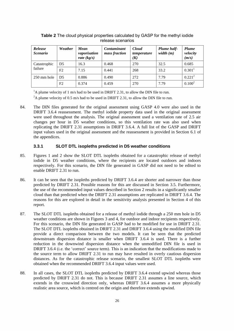
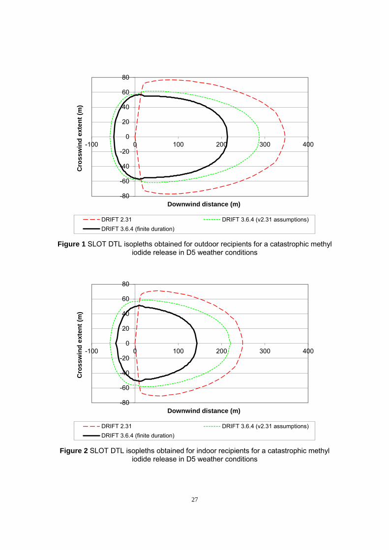
85. Figures 1 and 2 show the SLOT DTL isopleths obtained for a catastrophic release of methyl
iodide in D5 weather conditions, where the recipients are located outdoors and indoors
respectively. For this scenario, the DIN file generated in GASP did not need to be edited to
enable DRIFT 2.31 to run.
86. It can be seen that the isopleths predicted by DRIFT 3.6.4 are shorter and narrower than those
predicted by DRIFT 2.31. Possible reasons for this are discussed in Section 3.5. Furthermore,
the use of the recommended input values described in Section 2 results in a significantly smaller
cloud than that predicted when the DRIFT 2.31 assumptions are replicated in DRIFT 3.6.4. The
reasons for this are explored in detail in the sensitivity analysis presented in Section 4 of this
report.
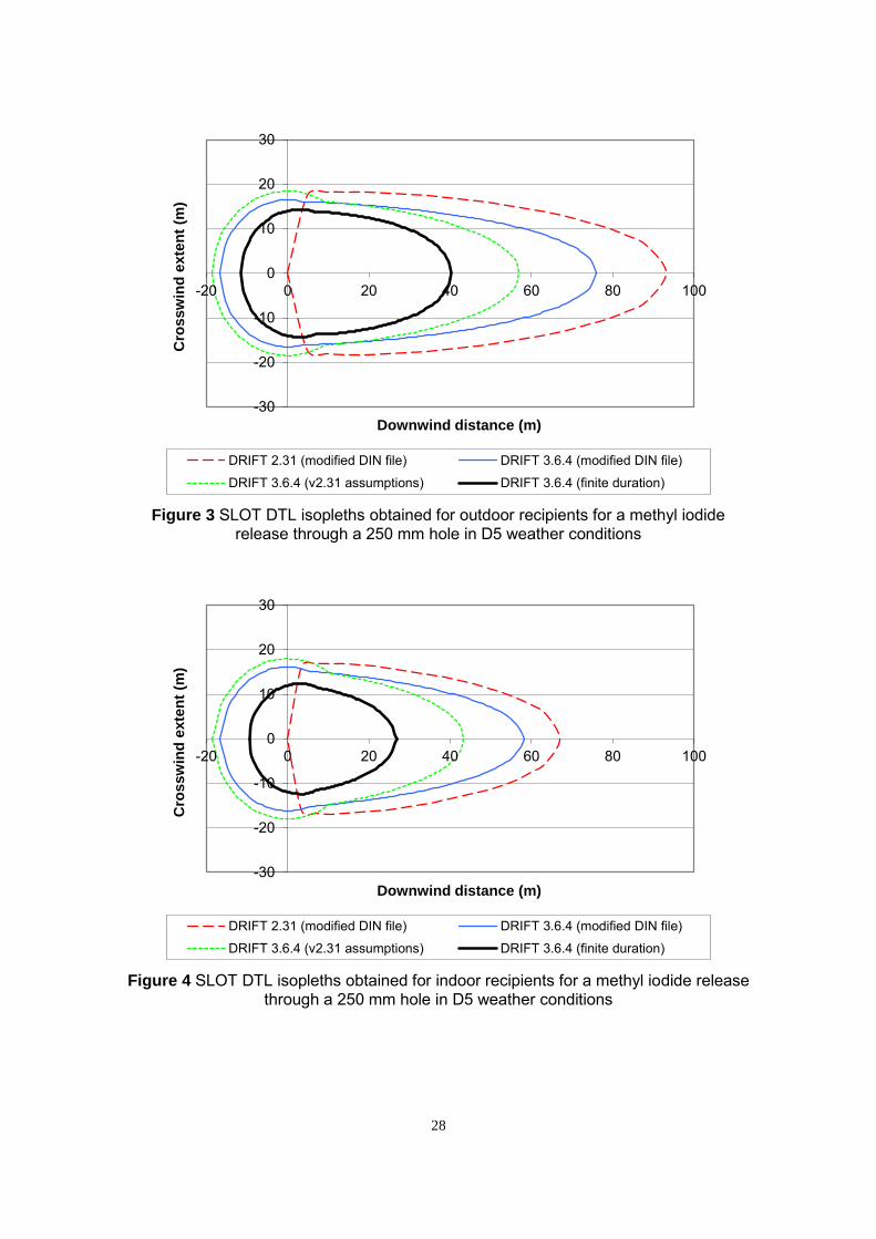
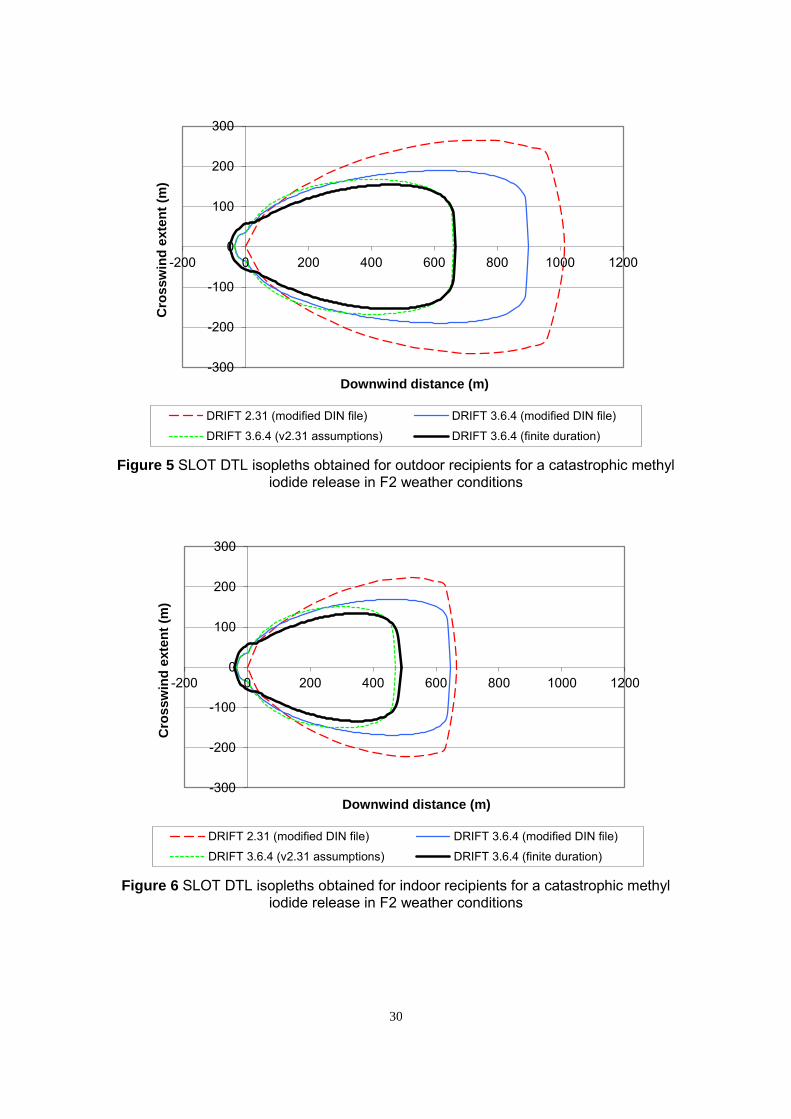
87. The SLOT DTL isopleths obtained for a release of methyl iodide through a 250 mm hole in D5
weather conditions are shown in Figures 3 and 4, for outdoor and indoor recipients respectively.
For this scenario, the DIN file generated in GASP had to be modified for use in DRIFT 2.31.
The SLOT DTL isopleths obtained in DRIFT 2.31 and DRIFT 3.6.4 using the modified DIN file
provide a direct comparison between the two models. It can be seen that the predicted
downstream dispersion distance is smaller when DRIFT 3.6.4 is used. There is a further
reduction in the downwind dispersion distance when the unmodified DIN file is used in
DRIFT 3.6.4 (i.e. the ‘correct’ source term). This is an indication that the modifications made to
the source term to allow DRIFT 2.31 to run may have resulted in overly cautious dispersion
distances. As for the catastrophic release scenario, the smallest SLOT DTL isopleths were
obtained when the recommended DRIFT 3.6.4 input values were used.
88. In all cases, the SLOT DTL isopleths predicted by DRIFT 3.6.4 extend upwind whereas those
predicted by DRIFT 2.31 do not. This is because DRIFT 2.31 assumes a line source, which
extends in the crosswind direction only, whereas DRIFT 3.6.4 assumes a more physically
realistic area source, which is centred on the origin and therefore extends upwind.
27
Figure 1 SLOT DTL isopleths obtained for outdoor recipients for a catastrophic methyl iodide release in D5 weather conditions
Figure 2 SLOT DTL isopleths obtained for indoor recipients for a catastrophic methyl iodide release in D5 weather conditions
-80
-60
-40
-20
0
20
40
60
80
-100 0 100 200 300 400
Cro
ssw
ind
exte
nt
(m)
Downwind distance (m)
DRIFT 2.31 DRIFT 3.6.4 (v2.31 assumptions)DRIFT 3.6.4 (finite duration)
-80
-60
-40
-20
0
20
40
60
80
-100 0 100 200 300 400
Cro
ssw
ind
exte
nt
(m)
Downwind distance (m)
DRIFT 2.31 DRIFT 3.6.4 (v2.31 assumptions)DRIFT 3.6.4 (finite duration)
28
Figure 3 SLOT DTL isopleths obtained for outdoor recipients for a methyl iodide release through a 250 mm hole in D5 weather conditions
Figure 4 SLOT DTL isopleths obtained for indoor recipients for a methyl iodide release through a 250 mm hole in D5 weather conditions
-30
-20
-10
0
10
20
30
-20 0 20 40 60 80 100
Cro
ssw
ind
exte
nt
(m)
Downwind distance (m)
DRIFT 2.31 (modified DIN file) DRIFT 3.6.4 (modified DIN file)
DRIFT 3.6.4 (v2.31 assumptions) DRIFT 3.6.4 (finite duration)
-30
-20
-10
0
10
20
30
-20 0 20 40 60 80 100
Cro
ssw
ind
exte
nt
(m)
Downwind distance (m)
DRIFT 2.31 (modified DIN file) DRIFT 3.6.4 (modified DIN file)
DRIFT 3.6.4 (v2.31 assumptions) DRIFT 3.6.4 (finite duration)

29
3.3.2 SLOT DTL isopleths predicted in F2 weather conditions
89. Figures 5 and 6 show the SLOT DTL isopleths obtained for a catastrophic release of methyl
iodide in F2 weather conditions, where the recipients are located outdoors and indoors
respectively. For this scenario, the DIN file generated in GASP had to be edited for use in
DRIFT 2.31.
90. As for D5 weather conditions, the SLOT DTL isopleths predicted by DRIFT 2.31 are larger
than those predicted by DRIFT 3.6.4. When the scenarios are modelled in DRIFT 3.6.4, the
largest isopleths are obtained when the modified DIN file is used. This is to be expected, since
the modified DIN file contains a lower surface roughness length and a higher plume velocity
than the unmodified file.
91. The SLOT DTL isopleths obtained when DRIFT 3.6.4 is used to replicate the DRIFT 2.31
assumptions are similar in size to those obtained when DRIFT 3.6.4 is run using the
assumptions recommended in Section 2. However, use of the recommended assumptions
produces isopleths that are larger above the source. The reasons for this are discussed in the
sensitivity analysis presented in Section 4 of this report.
92. The SLOT DTL isopleths obtained for a release of methyl iodide through a 250 mm hole in F2
weather conditions are shown in Figures 7 and 8, for outdoor and indoor recipients respectively.
For this scenario, the DIN file generated in GASP had to be modified for use in DRIFT 2.31. It
can be seen that the isopleths obtained using the modified DIN file (using both DRIFT 2.31 and
DRIFT 3.6.4) are significantly larger than those obtained when using the unmodified DIN file in
DRIFT 3.6.4. This clearly illustrates that for this scenario, the modified source term is not a
good representation of the actual release.
30
Figure 5 SLOT DTL isopleths obtained for outdoor recipients for a catastrophic methyl iodide release in F2 weather conditions
Figure 6 SLOT DTL isopleths obtained for indoor recipients for a catastrophic methyl iodide release in F2 weather conditions
-300
-200
-100
0
100
200
300
-200 0 200 400 600 800 1000 1200
Cro
ssw
ind
exte
nt
(m)
Downwind distance (m)
DRIFT 2.31 (modified DIN file) DRIFT 3.6.4 (modified DIN file)
DRIFT 3.6.4 (v2.31 assumptions) DRIFT 3.6.4 (finite duration)
-300
-200
-100
0
100
200
300
-200 0 200 400 600 800 1000 1200
Cro
ssw
ind
exte
nt
(m)
Downwind distance (m)
DRIFT 2.31 (modified DIN file) DRIFT 3.6.4 (modified DIN file)
DRIFT 3.6.4 (v2.31 assumptions) DRIFT 3.6.4 (finite duration)
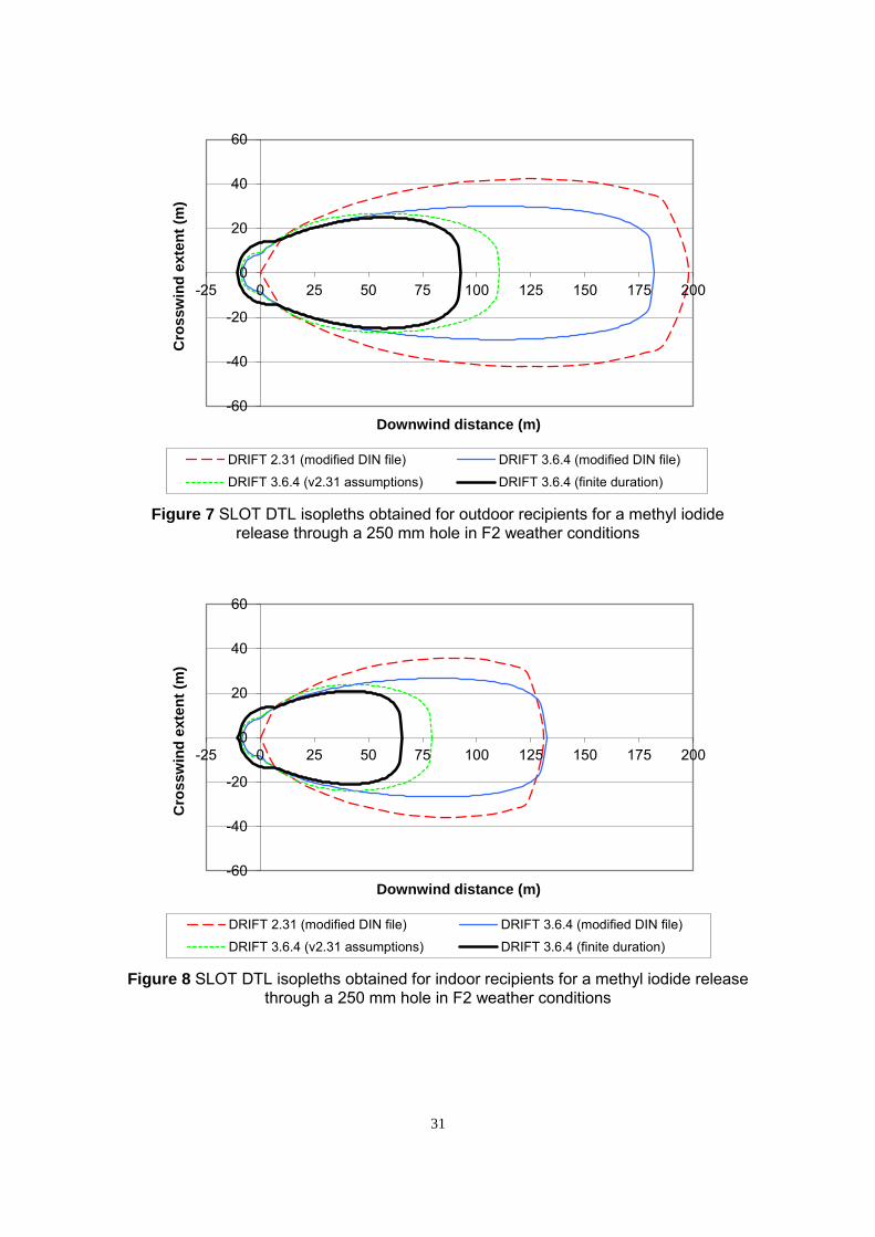
31
Figure 7 SLOT DTL isopleths obtained for outdoor recipients for a methyl iodiderelease through a 250 mm hole in F2 weather conditions
Figure 8 SLOT DTL isopleths obtained for indoor recipients for a methyl iodide releasethrough a 250 mm hole in F2 weather conditions
-60
-40
-20
0
20
40
60
-25 0 25 50 75 100 125 150 175 200
Cro
ssw
ind
exte
nt
(m)
Downwind distance (m)
DRIFT 2.31 (modified DIN file) DRIFT 3.6.4 (modified DIN file)
DRIFT 3.6.4 (v2.31 assumptions) DRIFT 3.6.4 (finite duration)
-60
-40
-20
0
20
40
60
-25 0 25 50 75 100 125 150 175 200
Cro
ssw
ind
exte
nt
(m)
Downwind distance (m)
DRIFT 2.31 (modified DIN file) DRIFT 3.6.4 (modified DIN file)
DRIFT 3.6.4 (v2.31 assumptions) DRIFT 3.6.4 (finite duration)
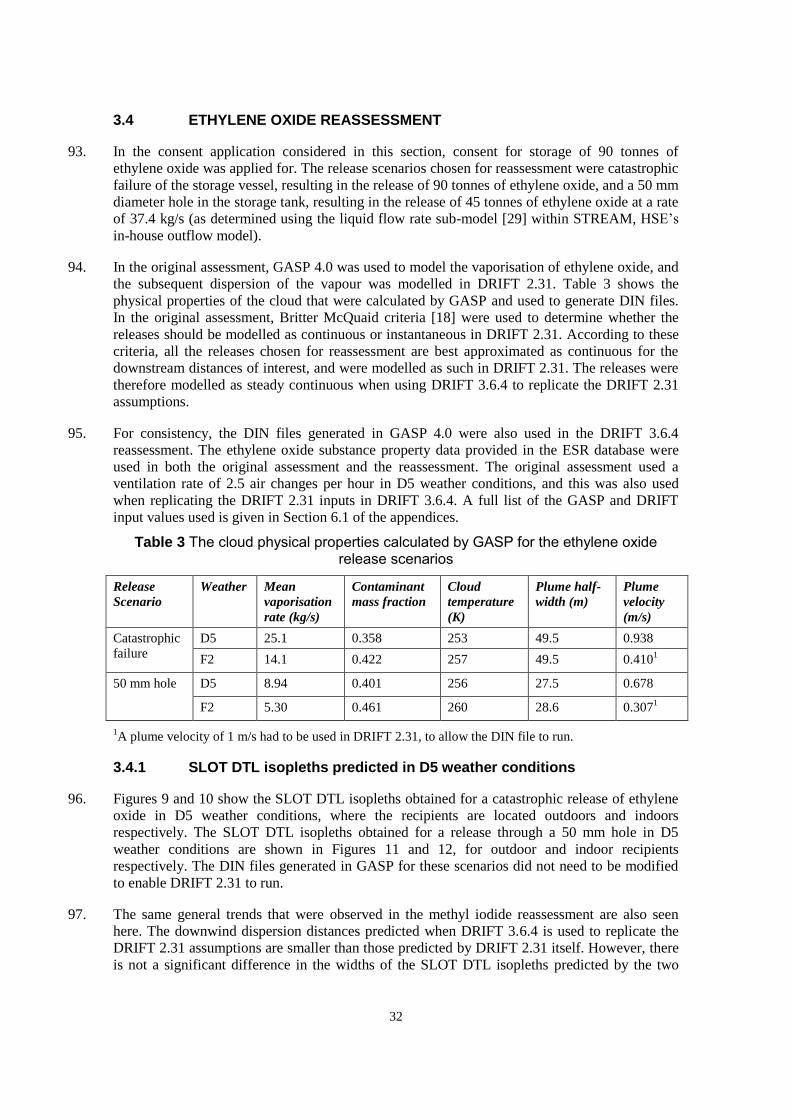
32
3.4 ETHYLENE OXIDE REASSESSMENT
93. In the consent application considered in this section, consent for storage of 90 tonnes of
ethylene oxide was applied for. The release scenarios chosen for reassessment were catastrophic
failure of the storage vessel, resulting in the release of 90 tonnes of ethylene oxide, and a 50 mm
diameter hole in the storage tank, resulting in the release of 45 tonnes of ethylene oxide at a rate
of 37.4 kg/s (as determined using the liquid flow rate sub-model [29] within STREAM, HSE’s
in-house outflow model).
94. In the original assessment, GASP 4.0 was used to model the vaporisation of ethylene oxide, and
the subsequent dispersion of the vapour was modelled in DRIFT 2.31. Table 3 shows the
physical properties of the cloud that were calculated by GASP and used to generate DIN files.
In the original assessment, Britter McQuaid criteria [18] were used to determine whether the
releases should be modelled as continuous or instantaneous in DRIFT 2.31. According to these
criteria, all the releases chosen for reassessment are best approximated as continuous for the
downstream distances of interest, and were modelled as such in DRIFT 2.31. The releases were
therefore modelled as steady continuous when using DRIFT 3.6.4 to replicate the DRIFT 2.31
assumptions.
95. For consistency, the DIN files generated in GASP 4.0 were also used in the DRIFT 3.6.4
reassessment. The ethylene oxide substance property data provided in the ESR database were
used in both the original assessment and the reassessment. The original assessment used a
ventilation rate of 2.5 air changes per hour in D5 weather conditions, and this was also used
when replicating the DRIFT 2.31 inputs in DRIFT 3.6.4. A full list of the GASP and DRIFT
input values used is given in Section 6.1 of the appendices.
Table 3 The cloud physical properties calculated by GASP for the ethylene oxide release scenarios
Release
Scenario
Weather Mean
vaporisation
rate (kg/s)
Contaminant
mass fraction
Cloud
temperature
(K)
Plume half-
width (m)
Plume
velocity
(m/s)
Catastrophic
failure
D5 25.1 0.358 253 49.5 0.938
F2 14.1 0.422 257 49.5 0.4101
50 mm hole D5 8.94 0.401 256 27.5 0.678
F2 5.30 0.461 260 28.6 0.3071
1A plume velocity of 1 m/s had to be used in DRIFT 2.31, to allow the DIN file to run.
3.4.1 SLOT DTL isopleths predicted in D5 weather conditions
96. Figures 9 and 10 show the SLOT DTL isopleths obtained for a catastrophic release of ethylene
oxide in D5 weather conditions, where the recipients are located outdoors and indoors
respectively. The SLOT DTL isopleths obtained for a release through a 50 mm hole in D5
weather conditions are shown in Figures 11 and 12, for outdoor and indoor recipients
respectively. The DIN files generated in GASP for these scenarios did not need to be modified
to enable DRIFT 2.31 to run.
97. The same general trends that were observed in the methyl iodide reassessment are also seen
here. The downwind dispersion distances predicted when DRIFT 3.6.4 is used to replicate the
DRIFT 2.31 assumptions are smaller than those predicted by DRIFT 2.31 itself. However, there
is not a significant difference in the widths of the SLOT DTL isopleths predicted by the two
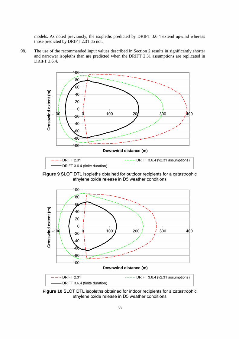
33
models. As noted previously, the isopleths predicted by DRIFT 3.6.4 extend upwind whereas
those predicted by DRIFT 2.31 do not.
98. The use of the recommended input values described in Section 2 results in significantly shorter
and narrower isopleths than are predicted when the DRIFT 2.31 assumptions are replicated in
DRIFT 3.6.4.
Figure 9 SLOT DTL isopleths obtained for outdoor recipients for a catastrophicethylene oxide release in D5 weather conditions
Figure 10 SLOT DTL isopleths obtained for indoor recipients for a catastrophicethylene oxide release in D5 weather conditions
-100
-80
-60
-40
-20
0
20
40
60
80
100
-100 0 100 200 300 400
Cro
ssw
ind
exte
nt
(m)
Downwind distance (m)
DRIFT 2.31 DRIFT 3.6.4 (v2.31 assumptions)DRIFT 3.6.4 (finite duration)
-100
-80
-60
-40
-20
0
20
40
60
80
100
-100 0 100 200 300 400
Cro
ssw
ind
exte
nt
(m)
Downwind distance (m)
DRIFT 2.31 DRIFT 3.6.4 (v2.31 assumptions)DRIFT 3.6.4 (finite duration)
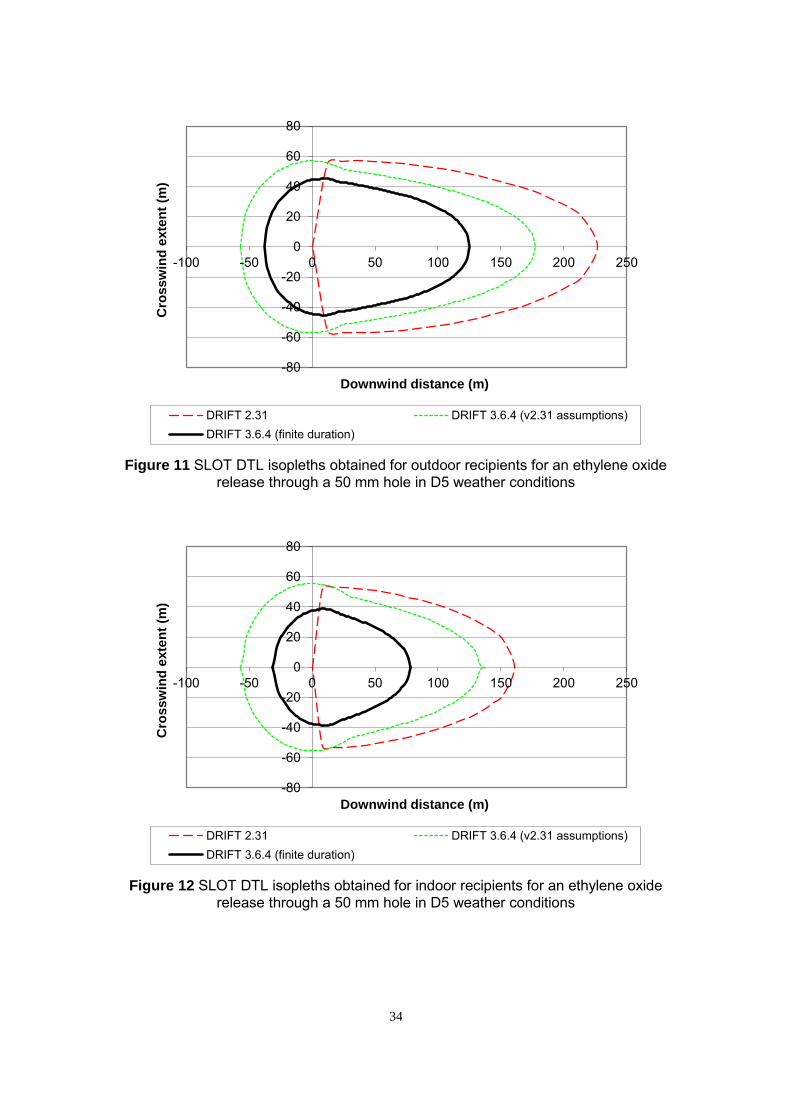
34
Figure 11 SLOT DTL isopleths obtained for outdoor recipients for an ethylene oxide release through a 50 mm hole in D5 weather conditions
Figure 12 SLOT DTL isopleths obtained for indoor recipients for an ethylene oxide release through a 50 mm hole in D5 weather conditions
-80
-60
-40
-20
0
20
40
60
80
-100 -50 0 50 100 150 200 250
Cro
ssw
ind
exte
nt
(m)
Downwind distance (m)
DRIFT 2.31 DRIFT 3.6.4 (v2.31 assumptions)DRIFT 3.6.4 (finite duration)
-80
-60
-40
-20
0
20
40
60
80
-100 -50 0 50 100 150 200 250
Cro
ssw
ind
exte
nt
(m)
Downwind distance (m)
DRIFT 2.31 DRIFT 3.6.4 (v2.31 assumptions)DRIFT 3.6.4 (finite duration)
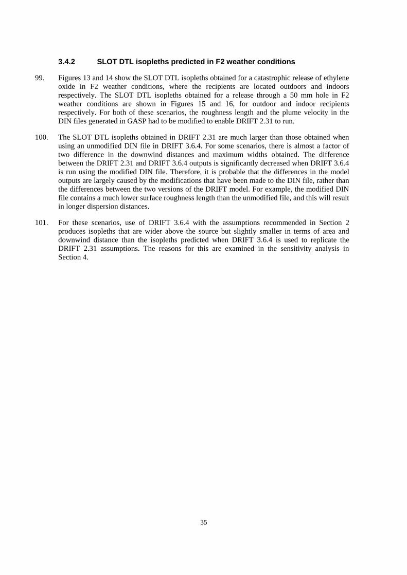
35
3.4.2 SLOT DTL isopleths predicted in F2 weather conditions
99. Figures 13 and 14 show the SLOT DTL isopleths obtained for a catastrophic release of ethylene
oxide in F2 weather conditions, where the recipients are located outdoors and indoors
respectively. The SLOT DTL isopleths obtained for a release through a 50 mm hole in F2
weather conditions are shown in Figures 15 and 16, for outdoor and indoor recipients
respectively. For both of these scenarios, the roughness length and the plume velocity in the
DIN files generated in GASP had to be modified to enable DRIFT 2.31 to run.
100. The SLOT DTL isopleths obtained in DRIFT 2.31 are much larger than those obtained when
using an unmodified DIN file in DRIFT 3.6.4. For some scenarios, there is almost a factor of
two difference in the downwind distances and maximum widths obtained. The difference
between the DRIFT 2.31 and DRIFT 3.6.4 outputs is significantly decreased when DRIFT 3.6.4
is run using the modified DIN file. Therefore, it is probable that the differences in the model
outputs are largely caused by the modifications that have been made to the DIN file, rather than
the differences between the two versions of the DRIFT model. For example, the modified DIN
file contains a much lower surface roughness length than the unmodified file, and this will result
in longer dispersion distances.
101. For these scenarios, use of DRIFT 3.6.4 with the assumptions recommended in Section 2
produces isopleths that are wider above the source but slightly smaller in terms of area and
downwind distance than the isopleths predicted when DRIFT 3.6.4 is used to replicate the
DRIFT 2.31 assumptions. The reasons for this are examined in the sensitivity analysis in
Section 4.
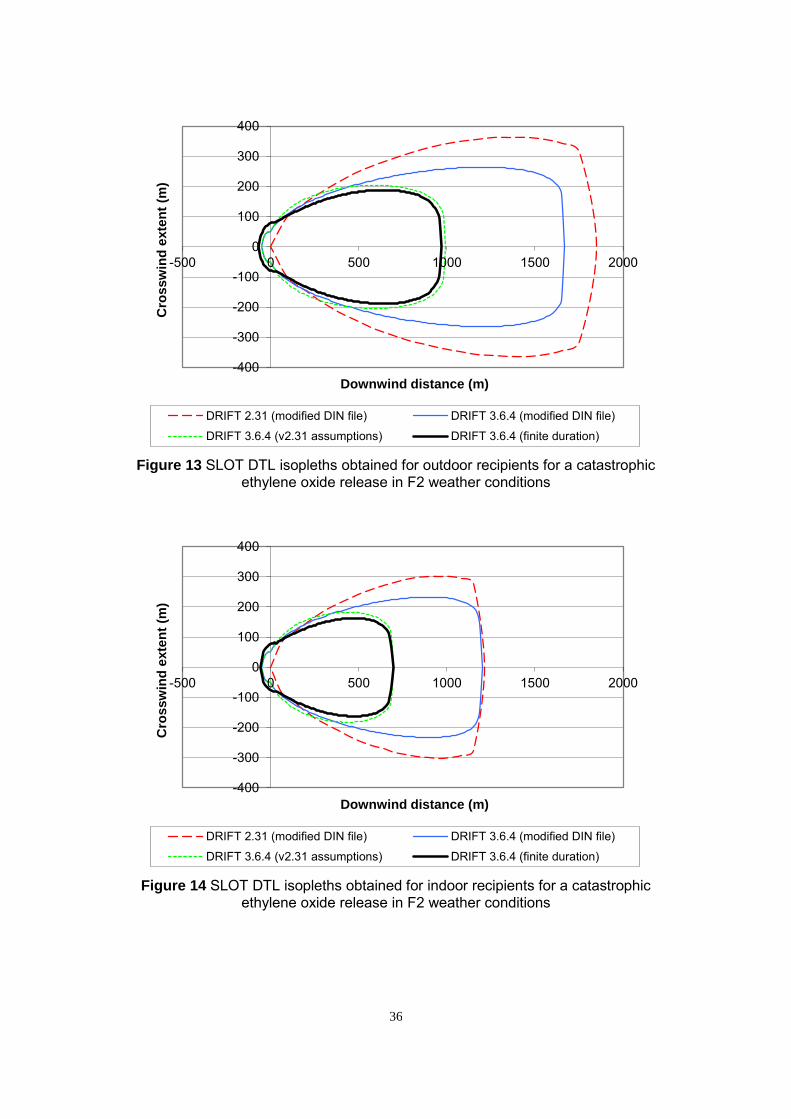
36
Figure 13 SLOT DTL isopleths obtained for outdoor recipients for a catastrophicethylene oxide release in F2 weather conditions
Figure 14 SLOT DTL isopleths obtained for indoor recipients for a catastrophicethylene oxide release in F2 weather conditions
-400
-300
-200
-100
0
100
200
300
400
-500 0 500 1000 1500 2000
Cro
ssw
ind
exte
nt
(m)
Downwind distance (m)
DRIFT 2.31 (modified DIN file) DRIFT 3.6.4 (modified DIN file)
DRIFT 3.6.4 (v2.31 assumptions) DRIFT 3.6.4 (finite duration)
-400
-300
-200
-100
0
100
200
300
400
-500 0 500 1000 1500 2000
Cro
ssw
ind
exte
nt
(m)
Downwind distance (m)
DRIFT 2.31 (modified DIN file) DRIFT 3.6.4 (modified DIN file)
DRIFT 3.6.4 (v2.31 assumptions) DRIFT 3.6.4 (finite duration)
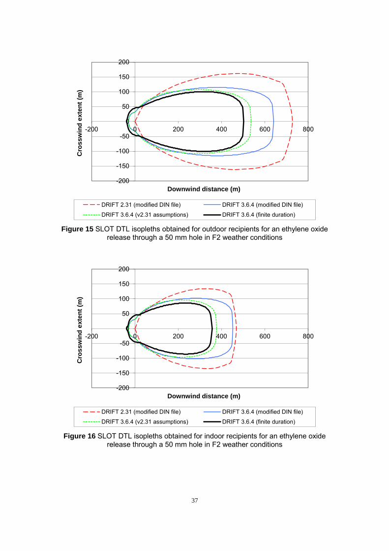
37
Figure 15 SLOT DTL isopleths obtained for outdoor recipients for an ethylene oxide release through a 50 mm hole in F2 weather conditions
Figure 16 SLOT DTL isopleths obtained for indoor recipients for an ethylene oxide release through a 50 mm hole in F2 weather conditions
-200
-150
-100
-50
0
50
100
150
200
-200 0 200 400 600 800
Cro
ssw
ind
exte
nt
(m)
Downwind distance (m)
DRIFT 2.31 (modified DIN file) DRIFT 3.6.4 (modified DIN file)
DRIFT 3.6.4 (v2.31 assumptions) DRIFT 3.6.4 (finite duration)
-200
-150
-100
-50
0
50
100
150
200
-200 0 200 400 600 800
Cro
ssw
ind
exte
nt
(m)
Downwind distance (m)
DRIFT 2.31 (modified DIN file) DRIFT 3.6.4 (modified DIN file)
DRIFT 3.6.4 (v2.31 assumptions) DRIFT 3.6.4 (finite duration)
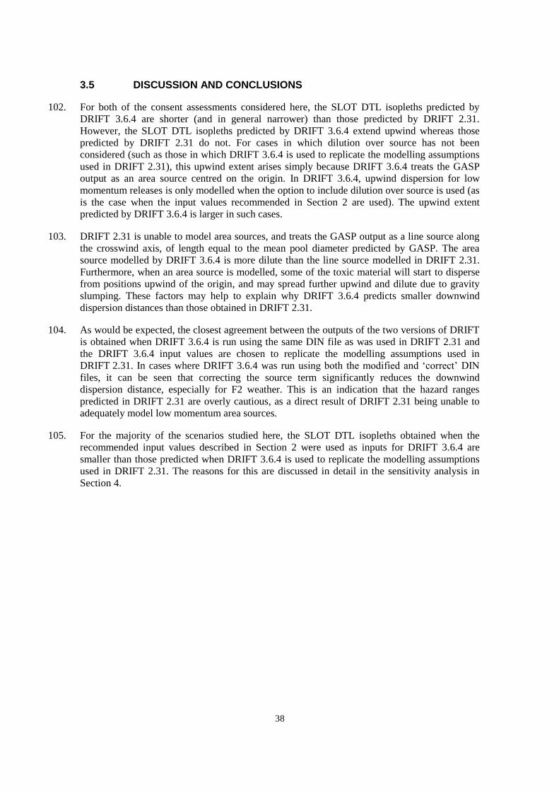
38
3.5 DISCUSSION AND CONCLUSIONS
102. For both of the consent assessments considered here, the SLOT DTL isopleths predicted by
DRIFT 3.6.4 are shorter (and in general narrower) than those predicted by DRIFT 2.31.
However, the SLOT DTL isopleths predicted by DRIFT 3.6.4 extend upwind whereas those
predicted by DRIFT 2.31 do not. For cases in which dilution over source has not been
considered (such as those in which DRIFT 3.6.4 is used to replicate the modelling assumptions
used in DRIFT 2.31), this upwind extent arises simply because DRIFT 3.6.4 treats the GASP
output as an area source centred on the origin. In DRIFT 3.6.4, upwind dispersion for low
momentum releases is only modelled when the option to include dilution over source is used (as
is the case when the input values recommended in Section 2 are used). The upwind extent
predicted by DRIFT 3.6.4 is larger in such cases.
103. DRIFT 2.31 is unable to model area sources, and treats the GASP output as a line source along
the crosswind axis, of length equal to the mean pool diameter predicted by GASP. The area
source modelled by DRIFT 3.6.4 is more dilute than the line source modelled in DRIFT 2.31.
Furthermore, when an area source is modelled, some of the toxic material will start to disperse
from positions upwind of the origin, and may spread further upwind and dilute due to gravity
slumping. These factors may help to explain why DRIFT 3.6.4 predicts smaller downwind
dispersion distances than those obtained in DRIFT 2.31.
104. As would be expected, the closest agreement between the outputs of the two versions of DRIFT
is obtained when DRIFT 3.6.4 is run using the same DIN file as was used in DRIFT 2.31 and
the DRIFT 3.6.4 input values are chosen to replicate the modelling assumptions used in
DRIFT 2.31. In cases where DRIFT 3.6.4 was run using both the modified and ‘correct’ DIN
files, it can be seen that correcting the source term significantly reduces the downwind
dispersion distance, especially for F2 weather. This is an indication that the hazard ranges
predicted in DRIFT 2.31 are overly cautious, as a direct result of DRIFT 2.31 being unable to
adequately model low momentum area sources.
105. For the majority of the scenarios studied here, the SLOT DTL isopleths obtained when the
recommended input values described in Section 2 were used as inputs for DRIFT 3.6.4 are
smaller than those predicted when DRIFT 3.6.4 is used to replicate the modelling assumptions
used in DRIFT 2.31. The reasons for this are discussed in detail in the sensitivity analysis in
Section 4.
39
4 SENSITIVITY ANALYSIS
4.1 INTRODUCTION
106. For the majority of the release scenarios modelled in Section 3, it was noted that the hazard
ranges predicted by DRIFT 3.6.4 significantly decrease in size when the recommended input
values described in Section 2 are used instead of input values equivalent to those used in
DRIFT 2.31. A detailed sensitivity analysis has been carried out to determine which of the new
modelling assumptions has the greatest effect on the model output. These sensitivity studies are
described in this section, and possible reasons for the differences in the hazard ranges are
presented.
4.2 METHODOLOGY
107. The sensitivity studies presented here are based on the methyl iodide and ethylene oxide release
scenarios described in Section 3. In each analysis, the base case is the DRIFT 3.6.4 run in which
the finite duration model has been used, together with the input values and assumptions
recommended in Section 2. The values used for a number of key inputs have been varied
individually. Table 4 lists the recommended values for these inputs and the variations used in
the sensitivity analysis. Each variation returns the input to the value used previously in
DRIFT 2.31.
Table 4 Assumptions used for sensitivity analysis
Parameter Recommended
DRIFT 3.6.4 input
values (base case)
Sensitivity
Release type Finite duration Continuous
Source dilution On Off
Plume meander (averaging time) 1800 s Off
Receiver height Centreline height 0 m
4.2.1 Graphical representation of the SLOT DTL isopleths
108. The following SLOT DTL isopleths were calculated in DRIFT 3.6.4 for each release scenario:
(a) The SLOT DTL isopleth calculated using the input values recommended in Section 2 of
this report. This is the base case and is represented by a bold black line in the figures,
labelled ‘base case’.
(b) The SLOT DTL isopleth calculated as for case (a), but modelling the release as
continuous rather than finite duration. In the figures, this case is labelled ‘release type:
continuous’ and is represented by a dashed red line.
(c) The SLOT DTL isopleth calculated as for case (a), except that the option to include
dilution over source is switched off. In the figures, this case is labelled ‘source dilution:
off’ and is represented by a solid blue line.
(d) The SLOT DTL isopleth calculated as for case (a), except that the option to include the
effects of plume meander is switched off. In the figures, this case is labelled ‘plume
meander: off’ and is represented by a dotted green line.
40
(e) The SLOT DTL isopleth calculated as for case (a), except that the receiver height is set
to 0 m, rather than the cloud centreline height. This comparison is included in the
methyl iodide sensitivity analysis only. In the figures, this case is labelled ‘receiver
height: 0 m’ and is represented by a dash-dot orange line.
4.3 METHYL IODIDE SENSITIVITY ANALYSIS
4.3.1 SLOT DTL isopleths predicted in D5 weather conditions
109. Figures 17 and 18 show the SLOT DTL isopleths obtained for a catastrophic release of methyl
iodide in D5 weather conditions, where the recipients are located outdoors and indoors
respectively. Figures 19 and 20 show the SLOT DTL isopleths obtained for a release of methyl
iodide through a 250 mm hole in D5 weather conditions, for outdoor and indoor recipients
respectively. These scenarios are considered together because the sensitivity analyses reveal the
same overall trends.
110. In each figure, isopleths corresponding to the base case and the four test cases described in
Section 4.2 are shown. The overall shape of the isopleths is not significantly affected by any of
the sensitivity tests, and none of the test cases produce SLOT DTL isopleths smaller than those
obtained in the base case. For both scenarios (and both types of recipient), the largest increase in
the size of the SLOT DTL isopleths is observed when the option to include dilution over source
is switched off: the width and the upwind and downwind extent all increase when the effects of
dilution over source are neglected.
111. Changing the release type from finite duration to steady continuous has little effect on the SLOT
DTL isopleths for either scenario.
112. There is a noticeable increase in the downwind extent of the SLOT DTL isopleths for outdoor
recipients when the option to include the effects of plume meander is switched off. However,
there is no accompanying increase in the upwind extent or the width of the isopleths. For indoor
recipients, neglecting the effects of plume meander results in a smaller increase in the maximum
downwind distance to the SLOT DTL.
113. Setting the receiver height to 0 m instead of the cloud centreline height has no effect on the
SLOT DTL isopleths for indoor or outdoor recipients for either scenario.
114. Explanations for these observations are provided in Section 4.5.

41
Figure 17 Sensitivity analysis of the SLOT DTL isopleths obtained for outdoor recipients for a catastrophic methyl iodide release in D5 weather conditions. The cases with a receiver height of 0 m and a release type of continuous give similar isopleths to
the base case.
Figure 18 Sensitivity analysis of the SLOT DTL isopleths obtained for indoor recipients for a catastrophic methyl iodide release in D5 weather conditions. The cases with a receiver height of 0 m and a release type of continuous give similar isopleths to the
base case.
-80
-60
-40
-20
0
20
40
60
80
-100 -50 0 50 100 150 200 250 300
Cro
ssw
ind
exte
nt
(m)
Downwind distance (m)
Base case Receiver height: 0 mSource dilution: off Plume meander: offRelease type: continuous
-80
-60
-40
-20
0
20
40
60
80
-100 -50 0 50 100 150 200 250 300
Cro
ssw
ind
exte
nt
(m)
Downwind distance (m)
Base case Receiver height: 0 mSource dilution: off Plume meander: offRelease type: continuous
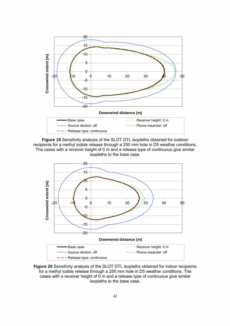
42
Figure 19 Sensitivity analysis of the SLOT DTL isopleths obtained for outdoor recipients for a methyl iodide release through a 250 mm hole in D5 weather conditions. The cases with a receiver height of 0 m and a release type of continuous give similar
isopleths to the base case.
Figure 20 Sensitivity analysis of the SLOT DTL isopleths obtained for indoor recipients for a methyl iodide release through a 250 mm hole in D5 weather conditions. The cases with a receiver height of 0 m and a release type of continuous give similar
isopleths to the base case.
-20
-15
-10
-5
0
5
10
15
20
-20 -10 0 10 20 30 40 50
Cro
ssw
ind
exte
nt
(m)
Downwind distance (m)
Base case Receiver height: 0 mSource dilution: off Plume meander: offRelease type: continuous
-20
-15
-10
-5
0
5
10
15
20
-20 -10 0 10 20 30 40 50
Cro
ssw
ind
exte
nt
(m)
Downwind distance (m)
Base case Receiver height: 0 mSource dilution: off Plume meander: offRelease type: continuous
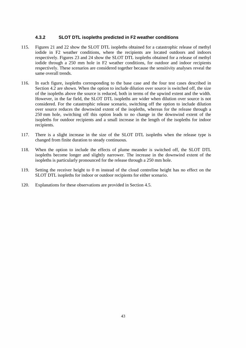
43
4.3.2 SLOT DTL isopleths predicted in F2 weather conditions
115. Figures 21 and 22 show the SLOT DTL isopleths obtained for a catastrophic release of methyl
iodide in F2 weather conditions, where the recipients are located outdoors and indoors
respectively. Figures 23 and 24 show the SLOT DTL isopleths obtained for a release of methyl
iodide through a 250 mm hole in F2 weather conditions, for outdoor and indoor recipients
respectively. These scenarios are considered together because the sensitivity analyses reveal the
same overall trends.
116. In each figure, isopleths corresponding to the base case and the four test cases described in
Section 4.2 are shown. When the option to include dilution over source is switched off, the size
of the isopleths above the source is reduced, both in terms of the upwind extent and the width.
However, in the far field, the SLOT DTL isopleths are wider when dilution over source is not
considered. For the catastrophic release scenario, switching off the option to include dilution
over source reduces the downwind extent of the isopleths, whereas for the release through a
250 mm hole, switching off this option leads to no change in the downwind extent of the
isopleths for outdoor recipients and a small increase in the length of the isopleths for indoor
recipients.
117. There is a slight increase in the size of the SLOT DTL isopleths when the release type is
changed from finite duration to steady continuous.
118. When the option to include the effects of plume meander is switched off, the SLOT DTL
isopleths become longer and slightly narrower. The increase in the downwind extent of the
isopleths is particularly pronounced for the release through a 250 mm hole.
119. Setting the receiver height to 0 m instead of the cloud centreline height has no effect on the
SLOT DTL isopleths for indoor or outdoor recipients for either scenario.
120. Explanations for these observations are provided in Section 4.5.
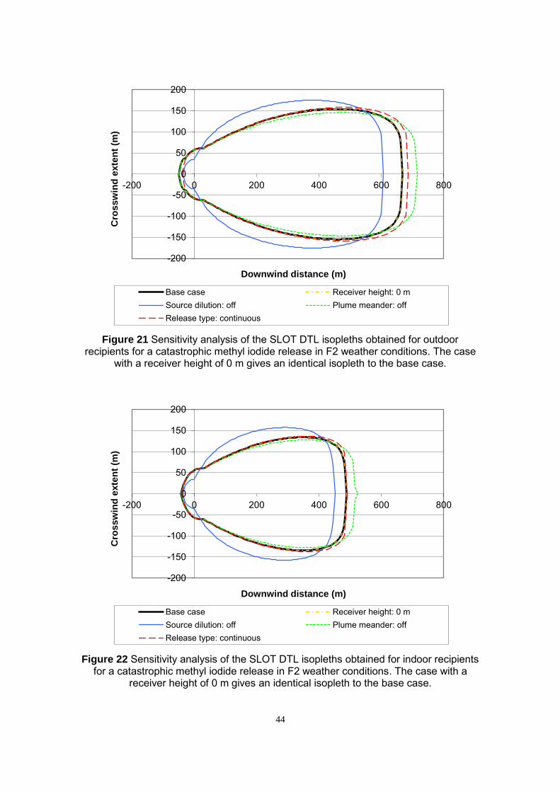
44
Figure 21 Sensitivity analysis of the SLOT DTL isopleths obtained for outdoor recipients for a catastrophic methyl iodide release in F2 weather conditions. The case
with a receiver height of 0 m gives an identical isopleth to the base case.
Figure 22 Sensitivity analysis of the SLOT DTL isopleths obtained for indoor recipients for a catastrophic methyl iodide release in F2 weather conditions. The case with a
receiver height of 0 m gives an identical isopleth to the base case.
-200
-150
-100
-50
0
50
100
150
200
-200 0 200 400 600 800
Cro
ssw
ind
exte
nt
(m)
Downwind distance (m)
Base case Receiver height: 0 mSource dilution: off Plume meander: offRelease type: continuous
-200
-150
-100
-50
0
50
100
150
200
-200 0 200 400 600 800
Cro
ssw
ind
exte
nt
(m)
Downwind distance (m)
Base case Receiver height: 0 mSource dilution: off Plume meander: offRelease type: continuous

45
Figure 23 Sensitivity analysis of the SLOT DTL isopleths obtained for outdoor recipients for a methyl iodide release through a 250 mm hole in F2 weather conditions. The cases with a receiver height of 0 m and a release type of continuous give similar
isopleths to the base case.
Figure 24 Sensitivity analysis of the SLOT DTL isopleths obtained for indoor recipients for a methyl iodide release through a 250 mm hole in F2 weather conditions. The cases with a receiver height of 0 m and a release type of continuous give similar isopleths to
the base case.
-40
-30
-20
-10
0
10
20
30
40
-20 0 20 40 60 80 100 120
Cro
ssw
ind
exte
nt
(m)
Downwind distance (m)
Base case Receiver height: 0 mSource dilution: off Plume meander: offRelease type: continuous
-40
-30
-20
-10
0
10
20
30
40
-20 0 20 40 60 80 100 120
Cro
ssw
ind
exte
nt
(m)
Downwind distance (m)
Base case Receiver height: 0 mSource dilution: off Plume meander: offRelease type: continuous

46
4.4 ETHYLENE OXIDE SENSITIVITY ANALYSIS
4.4.1 SLOT DTL isopleths predicted in D5 weather conditions
121. Figures 25 and 26 show the SLOT DTL isopleths obtained for a catastrophic release of ethylene
oxide in D5 weather conditions, where the recipients are located outdoors and indoors
respectively. Figures 27 and 28 show the SLOT DTL isopleths obtained for a release of
ethylene oxide through a 50 mm hole in D5 weather conditions, for outdoor and indoor
recipients respectively. These scenarios are considered together because the sensitivity analyses
reveal the same overall trends.
122. In each figure, isopleths corresponding to the base case and test cases (b) to (d) (as defined in
Section 4.2.1) are shown. Isopleths corresponding to a receiver height of 0 m have not been
calculated, because the methyl iodide sensitivity analysis revealed that changing the receiver
height from the cloud centreline height to 0 m had a negligible effect on the model output for
dense gas releases. The same trends were observed as in the methyl iodide sensitivity analysis,
but the key points are reproduced here for completeness.
123. The overall shape of the isopleths is not significantly affected by any of the sensitivity tests. For
both scenarios (and both types of recipient), the largest increase in the size of the SLOT DTL
isopleths is observed when the option to include dilution over source is switched off: the
maximum width of the isopleths and the upwind and downwind extent all increase when the
effects of dilution over source are neglected.
124. There is a slight increase in the downwind extent of the SLOT DTL isopleths when the option to
include the effects of plume meander is switched off. However, there is no accompanying
increase in the upwind extent or the width of the isopleths.
125. Changing the release type from finite duration to steady continuous has little effect on the SLOT
DTL isopleths for either scenario.
126. Explanations for these observations are provided in Section 4.5.
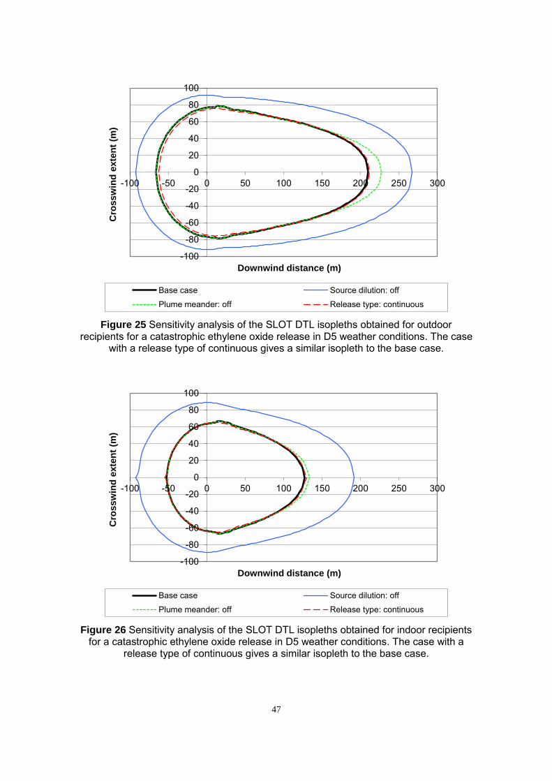
47
Figure 25 Sensitivity analysis of the SLOT DTL isopleths obtained for outdoor recipients for a catastrophic ethylene oxide release in D5 weather conditions. The case
with a release type of continuous gives a similar isopleth to the base case.
Figure 26 Sensitivity analysis of the SLOT DTL isopleths obtained for indoor recipients for a catastrophic ethylene oxide release in D5 weather conditions. The case with a
release type of continuous gives a similar isopleth to the base case.
-100
-80
-60
-40
-20
0
20
40
60
80
100
-100 -50 0 50 100 150 200 250 300
Cro
ssw
ind
exte
nt
(m)
Downwind distance (m)
Base case Source dilution: off
Plume meander: off Release type: continuous
-100
-80
-60
-40
-20
0
20
40
60
80
100
-100 -50 0 50 100 150 200 250 300
Cro
ssw
ind
exte
nt
(m)
Downwind distance (m)
Base case Source dilution: off
Plume meander: off Release type: continuous

48
Figure 27 Sensitivity analysis of the SLOT DTL isopleths obtained for outdoor recipients for an ethylene oxide release through a 50 mm hole in D5 weather
conditions. The case with a release type of continuous gives a similar isopleth to the base case.
Figure 28 Sensitivity analysis of the SLOT DTL isopleths obtained for indoor recipients for an ethylene oxide release through a 50 mm hole in D5 weather conditions. The
case with a release type of continuous gives a similar isopleth to the base case.
-80
-60
-40
-20
0
20
40
60
80
-100 -50 0 50 100 150 200
Cro
ssw
ind
exte
nt
(m)
Downwind distance (m)
Base case Source dilution: off
Plume meander: off Release type: continuous
-80
-60
-40
-20
0
20
40
60
80
-100 -50 0 50 100 150 200
Cro
ssw
ind
exte
nt
(m)
Downwind distance (m)
Base case Source dilution: off
Plume meander: off Release type: continuous
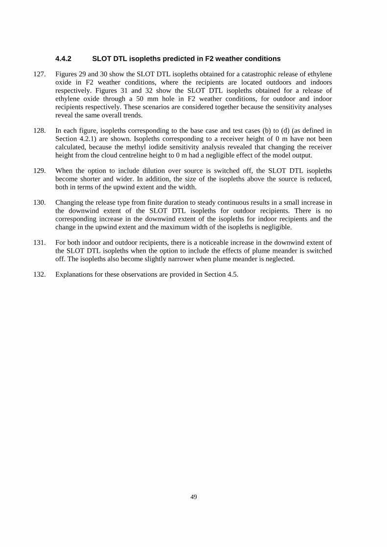
49
4.4.2 SLOT DTL isopleths predicted in F2 weather conditions
127. Figures 29 and 30 show the SLOT DTL isopleths obtained for a catastrophic release of ethylene
oxide in F2 weather conditions, where the recipients are located outdoors and indoors
respectively. Figures 31 and 32 show the SLOT DTL isopleths obtained for a release of
ethylene oxide through a 50 mm hole in F2 weather conditions, for outdoor and indoor
recipients respectively. These scenarios are considered together because the sensitivity analyses
reveal the same overall trends.
128. In each figure, isopleths corresponding to the base case and test cases (b) to (d) (as defined in
Section 4.2.1) are shown. Isopleths corresponding to a receiver height of 0 m have not been
calculated, because the methyl iodide sensitivity analysis revealed that changing the receiver
height from the cloud centreline height to 0 m had a negligible effect of the model output.
129. When the option to include dilution over source is switched off, the SLOT DTL isopleths
become shorter and wider. In addition, the size of the isopleths above the source is reduced,
both in terms of the upwind extent and the width.
130. Changing the release type from finite duration to steady continuous results in a small increase in
the downwind extent of the SLOT DTL isopleths for outdoor recipients. There is no
corresponding increase in the downwind extent of the isopleths for indoor recipients and the
change in the upwind extent and the maximum width of the isopleths is negligible.
131. For both indoor and outdoor recipients, there is a noticeable increase in the downwind extent of
the SLOT DTL isopleths when the option to include the effects of plume meander is switched
off. The isopleths also become slightly narrower when plume meander is neglected.
132. Explanations for these observations are provided in Section 4.5.
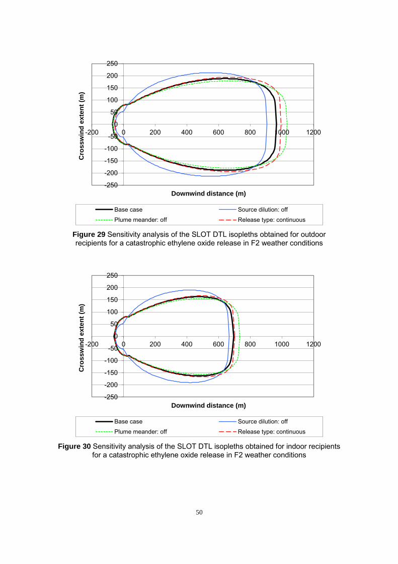
50
Figure 29 Sensitivity analysis of the SLOT DTL isopleths obtained for outdoorrecipients for a catastrophic ethylene oxide release in F2 weather conditions
Figure 30 Sensitivity analysis of the SLOT DTL isopleths obtained for indoor recipientsfor a catastrophic ethylene oxide release in F2 weather conditions
-250
-200
-150
-100
-50
0
50
100
150
200
250
-200 0 200 400 600 800 1000 1200
Cro
ssw
ind
exte
nt
(m)
Downwind distance (m)
Base case Source dilution: off
Plume meander: off Release type: continuous
-250
-200
-150
-100
-50
0
50
100
150
200
250
-200 0 200 400 600 800 1000 1200
Cro
ssw
ind
exte
nt
(m)
Downwind distance (m)
Base case Source dilution: off
Plume meander: off Release type: continuous
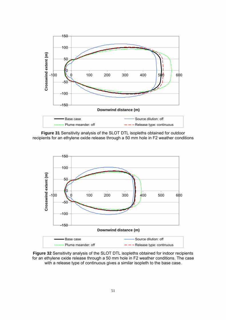
51
Figure 31 Sensitivity analysis of the SLOT DTL isopleths obtained for outdoor recipients for an ethylene oxide release through a 50 mm hole in F2 weather conditions
Figure 32 Sensitivity analysis of the SLOT DTL isopleths obtained for indoor recipients for an ethylene oxide release through a 50 mm hole in F2 weather conditions. The case
with a release type of continuous gives a similar isopleth to the base case.
-150
-100
-50
0
50
100
150
-100 0 100 200 300 400 500 600
Cro
ssw
ind
exte
nt
(m)
Downwind distance (m)
Base case Source dilution: off
Plume meander: off Release type: continuous
-150
-100
-50
0
50
100
150
-100 0 100 200 300 400 500 600
Cro
ssw
ind
exte
nt
(m)
Downwind distance (m)
Base case Source dilution: off
Plume meander: off Release type: continuous
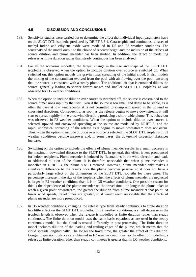
52
4.5 DISCUSSION AND CONCLUSIONS
133. Sensitivity studies were carried out to determine the effect that individual input parameters have
on the SLOT DTL isopleths predicted by DRIFT 3.6.4. Catastrophic and continuous releases of
methyl iodide and ethylene oxide were modelled in D5 and F2 weather conditions. The
sensitivity of the model output to the choice of receiver height and the inclusion of the effects of
source dilution and plume meander has been studied. In addition, the effect of modelling
releases as finite duration rather than steady continuous has been analysed.
134. For all the scenarios modelled, the largest change in the size and shape of the SLOT DTL
isopleths is observed when the option to include dilution over source is switched on. When
switched on, this option models the gravitational spreading of the initial cloud. It also models
the mixing of the contaminant evolved from the pool with air flowing over the pool, ensuring
that the source is consistent with a steady plume. The additional air that is entrained dilutes the
source, generally leading to shorter hazard ranges and smaller SLOT DTL isopleths, as was
observed for D5 weather conditions.
135. When the option to include dilution over source is switched off, the source is constrained to the
source dimensions input by the user. Even if the source is too small and dense to be stable, as is
often the case at low wind speeds, it is not permitted to slump and spread in the upwind or
crosswind directions. Consequently, as soon as the release begins to move downstream, it will
start to spread rapidly in the crosswind direction, producing a short, wide plume. This behaviour
was observed in F2 weather conditions. When the option to include dilution over source is
selected, upwind and crosswind spreading at the source are modelled by DRIFT 3, and the
rapid, unphysical spreading of the release as it begins to move downstream does not occur.
Thus, when the option to include dilution over source is selected, the SLOT DTL isopleths in F2
weather conditions become narrower and, in some cases, the downwind dispersion distances
increase.
136. Switching on the option to include the effects of plume meander results in a small decrease in
the maximum downwind distance to the SLOT DTL. In general, this effect is less pronounced
for indoor recipients. Plume meander is induced by fluctuations in the wind direction and leads
to additional dilution of the plume. It is therefore reasonable that when plume meander is
modelled in DRIFT 3, the plume size is reduced. However, plume meander only makes a
significant difference to the results once the plume becomes passive, so it does not have a
particularly large effect on the dimensions of the SLOT DTL isopleths for these cases. The
percentage increase in the size of the isopleths when the effects of plume meander are neglected
is larger in F2 weather conditions than it is in D5 weather conditions. One possible reason for
this is the dependence of the plume meander on the travel time: the longer the plume takes to
reach a given point downstream, the greater the dilution from plume meander at that point. At
lower wind speeds, travel times are greater, so it would seem reasonable that the effects of
plume meander are more pronounced.
137. In D5 weather conditions, changing the release type from steady continuous to finite duration
has little effect on the SLOT DTL isopleths. In F2 weather conditions, a small decrease in the
isopleth length is observed when the release is modelled as finite duration rather than steady
continuous. The finite duration model uses the same basic equations as are used in the steady
continuous model, but the cloud is treated differently in post-processing. The finite duration
model includes dilution of the leading and trailing edges of the plume, which means that the
cloud spreads longitudinally. The longer the travel time, the greater the effect of this dilution.
Longer dispersion distances are obtained in F2 weather conditions, so the effect of modelling a
release as finite duration rather than steady continuous is greater than in D5 weather conditions.

53
138. In Section 3, it was observed that for D5 weather conditions, the use of the recommended input
values described in Section 2 results in significantly smaller and narrower SLOT DTL isopleths
than those predicted when the DRIFT 2.31 assumptions are replicated in DRIFT 3.6.4. The
sensitivity analysis has revealed that the main reason for the decrease in the isopleth size is the
inclusion of the effects of source dilution, although the inclusion of the effects of plume
meander is also a contributing factor.
139. In F2 weather conditions, the SLOT DTL isopleths obtained when using the recommended
input values are generally only slightly smaller than the isopleths obtained when the
DRIFT 2.31 assumptions are replicated in DRIFT 3.6.4. Including the effects of plume meander
and (to a lesser degree) modelling the releases as finite duration rather than steady continuous
leads to a decrease in the size of the isopleths. However, in F2 weather conditions, the effect of
gravitational spreading over the source is also important. When the dilution over source option
is switched off, upwind gravitational spreading is not accounted for, leading to rapid crosswind
spreading at downstream locations and a wider plume downstream, but shorter range. However,
when the dilution over source option is switched on, the gravity spreading is more uniformly
distributed around the source, resulting in less rapid crosswind spreading downstream of the
source and longer, narrower isopleths. When moving from replicating the DRIFT 2.31
assumptions in DRIFT 3.6.4 to using the recommended input values described in Section 2, the
effects of plume meander and dilution over source counteract one another, leading to little
overall change in the size of the isopleths.
140. For the scenarios modelled in this sensitivity analysis, setting the receiver height to 0 m instead
of the cloud centreline height had a negligible effect on the SLOT DTL isopleths. Methyl iodide
and ethylene oxide are both dense gases, so the centreline height of the vapour cloud evolved
from a low momentum area source (such as a pool) will be close to 0 m at all dispersion
distances. Thus for these releases, both options result in the same receiver height and the SLOT
DTL isopleths are unaffected.
54
5 CONCLUSIONS
141. The DRIFT dispersion model was developed for HSE by ESR Technology. DRIFT version 3
has recently been released and contains many additions and modelling enhancements over the
version of DRIFT previously used by HSE (DRIFT 2.31). These include the extension of the
model to consider buoyant lift-off and buoyant rise, and the option to calculate initial dilution
over the source and upwind spreading. Finite duration and time varying releases can be
modelled in DRIFT 3, in addition to the instantaneous and steady continuous releases available
in DRIFT 2.31. The mathematical and scientific basis for the finite duration and time varying
models has been subject to expert peer review and found to be appropriate [13]. DRIFT 3 also
has an improved user interface, and is simpler and more intuitive to use than its predecessor,
DRIFT 2.31. It is compatible with HSE’s Substance Property Information (SPI) files.
142. HSE will use DRIFT 3 in its assessment of the hazards and risks posed by toxic and flammable
substances stored at major hazards sites. To ensure that DRIFT 3 is fit for purpose, a
programme of work is being undertaken at HSE. This includes an evaluation of the dispersion
modelling capabilities of DRIFT 3 [13] and an assessment of the performance of DRIFT 3 for
modelling the types of release scenario typically considered by HSE for Hazardous Substances
Consent assessments.
143. This report describes part of this programme of work and presents an assessment of the use of
DRIFT 3.6.4 for modelling the dispersion of vapour evolved from pools of toxic liquids. The
dispersion of such releases was previously modelled in DRIFT 2.31.
144. The proposed methodology for modelling the dispersion of vapour from pools of toxic using
DRIFT 3 has been described. These modelling recommendations were made in consultation
with the developers of the model and specialist inspectors and researchers within HSE. When a
change to the existing modelling methodology has been recommended, a justification of the
new approach has been provided. In most cases, differences between the modelling
methodologies used in DRIFT 2.31 and DRIFT 3 only arise because the enhanced modelling
capability of DRIFT 3 is being exploited to address particular physical effects believed to be
important for the modelled scenarios.
5.1 COMPARISON OF THE OUTPUTS OF DRIFT 2.31 AND DRIFT 3.6.4
145. Consent applications for methyl iodide and ethylene oxide that were originally assessed using
GASP and DRIFT 2.31 have been reassessed using GASP and DRIFT 3.6.4. The SLOT DTL
isopleths obtained in the original assessments and the reassessments have been compared, to
assess the impact of adopting DRIFT 3 on HSE’s land-use-planning advice.
146. The SLOT DTL isopleths predicted by DRIFT 3.6.4 are shorter (and in general narrower) than
those predicted by DRIFT 2.31. However, the SLOT DTL isopleths predicted by DRIFT 3.6.4
extend upwind whereas those predicted by DRIFT 2.31 do not.
147. It is possible that the difference between the SLOT DTL isopleths predicted by the two versions
of DRIFT is partly caused by the fact that DRIFT 2.31 is unable to model area sources.
DRIFT 2.31 treats the GASP output as a line source along the crosswind axis, of length equal to
the mean pool diameter predicted by GASP. The area source modelled by DRIFT 3.6.4 is
necessarily more dilute than the line source modelled in DRIFT 2.31. Furthermore, when an
area source is modelled, some of the toxic material will start to disperse from positions upwind
of the origin and may spread further upwind and dilute due to gravity spreading. These factors
may help to explain why DRIFT 3.6.4 predicts smaller downwind dispersion distances than
those obtained in DRIFT 2.31.

55
148. For some scenarios, DRIFT 2.31 cannot run using the cloud properties predicted by GASP, due
to shortcomings in its source model. In such cases, it is possible to manually modify the plume
velocity and roughness length in the DIN file so that DRIFT 2.31 can be run for the source
dimensions and vaporisation rate generated by GASP. However, using the edited source term
may not give a good representation of the dispersion from the pool. DRIFT 3 contains an
improved sub-model for low momentum area sources, which includes the effects of upwind
spreading. As a result, scenarios that would not run in DRIFT 2.31 usually run in DRIFT 3
without difficulty. As would be expected, the closest agreement between the outputs of the two
versions of DRIFT is obtained when DRIFT 3.6.4 is run using the same DIN file as was used in
DRIFT 2.31 and the DRIFT 3.6.4 input values are chosen to replicate the modelling
assumptions used in DRIFT 2.31. In cases where DRIFT 3.6.4 could be run using both the
modified and ‘correct’ DIN files, it can be seen that correcting the source term significantly
reduces the downwind dispersion distance, especially for F2 weather. This is an indication that
the hazard ranges predicted in DRIFT 2.31 are overly cautious, as a direct result of DRIFT 2.31
being unable to adequately model low momentum area sources.
5.2 SENSITIVITY ANALYSIS
149. A comparison was carried out between the DRIFT 3.6.4 outputs obtained when using the
recommended DRIFT 3 methodology for modelling the dispersion of vapour evolved from
pools of toxic liquids, and those obtained when replicating the DRIFT 2.31 assumptions.
Several changes have been made to the existing DRIFT 2.31 methodology, to make use of the
enhanced modelling capability of DRIFT 3. One such change is that the recommended DRIFT 3
methodology makes use of the new finite duration model, whereas when replicating the
DRIFT 2.31 assumptions, releases are modelled as steady continuous. In addition, the new
methodology recommends that the options to include the effects of dilution over source and
plume meander be switched on. DRIFT 2.31 did not have the facility to model these effects, so
these options are switched off when replicating the DRIFT 2.31 assumptions.
150. For the majority of the methyl iodide and ethylene oxide scenarios studied here, the SLOT DTL
isopleths obtained when using the recommended DRIFT 3 modelling methodology are smaller
than those predicted when DRIFT 3.6.4 is used to replicate the modelling assumptions used in
DRIFT 2.31. A detailed sensitivity analysis was carried out to determine which of the new
modelling assumptions has the greatest effect on the DRIFT 3 output.
151. For all the scenarios modelled, the largest change in the size and shape of the SLOT DTL
isopleths is observed when the option to include dilution over source is switched on. When
switched on, this option models the mixing of the contaminant evolved from the pool with air
flowing over the pool. The additional air that is entrained dilutes the source, generally leading to
shorter hazard ranges and smaller SLOT DTL isopleths.
152. Switching on the option to include the effects of plume meander results in a small decrease in
the maximum downwind distance to the SLOT DTL. In general, this effect is less pronounced
for indoor recipients. Plume meander is induced by fluctuations in the wind direction and leads
to additional dilution of the plume. It is therefore reasonable that when plume meander is
modelled in DRIFT, the plume size is reduced. However, plume meander only makes a
significant difference to the results once the plume becomes passive, so it does not have a
particularly large effect on the dimensions of the SLOT DTL isopleths.
153. In D5 weather conditions, changing the release type from steady continuous to finite duration
has little effect on the SLOT DTL isopleths. In F2 weather conditions, a small decrease in the
isopleth length is observed when the release is modelled as finite duration rather than steady
continuous. The finite duration model uses the same basic equations as are used in the steady
56
continuous model, but the cloud is treated differently in post-processing. The finite duration
model includes dilution of the leading and trailing edges of the plume, which means that the
cloud spreads longitudinally. The longer the travel time, the greater the effect of this dilution.
Longer dispersion distances are obtained in F2 weather conditions, so the effect of modelling a
release as finite duration rather than steady continuous is greater than in D5 weather conditions.
5.3 OUTCOMES
154. A number of modelling enhancements have been implemented in DRIFT 3, expanding the
scope and potential uses of the model [6, 7]. DRIFT 3.6.4 is therefore a significant improvement
on DRIFT 2.31, both in terms of the underlying science and in terms of user friendliness.
DRIFT 3.6.4 is generally more reliable and stable than DRIFT 2.31. It contains an improved
sub-model for low momentum area sources, which includes the effects of upwind spreading. As
a result, scenarios that would not run in DRIFT 2.31 usually run in DRIFT 3.6.4 without
difficulty.
155. DRIFT 3 contains a model for time varying releases, but this has not yet undergone thorough
evaluation so is not recommended for use in Hazardous Substances Consent assessments. HSE
therefore models the dispersion of vapour from pools of toxic liquids using the finite duration
option in DRIFT 3.6.4. The finite duration option accounts for dilution at the leading and
trailing edges of a dispersing plume and is expected to provide a better representation of the
physical processes that would occur during an actual release than the steady continuous model
in DRIFT 3 [6]. HSE also accounts for the effects of dilution over source and plume meander
when modelling the dispersion of vapour evolved from pools of toxic liquids in DRIFT 3.
156. As a result of this work and accompanying evaluation studies [13], DRIFT 3.6.4 has been
adopted by HSE to model the dispersion of vapour evolved from pools of toxic liquids for the
purposes of Hazardous Substances Consent assessment. DRIFT 2.31 is no longer to be used to
model such releases.
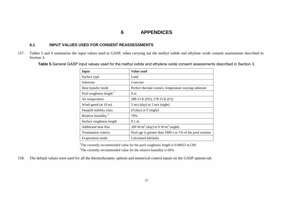
57
6 APPENDICES
6.1 INPUT VALUES USED FOR CONSENT REASSESSMENTS
157. Tables 5 and 6 summarise the input values used in GASP, when carrying out the methyl iodide and ethylene oxide consent assessments described in
Section 3.
Table 5 General GASP input values used for the methyl iodide and ethylene oxide consent assessments described in Section 3.
Input Value used
Surface type Land
Substrate Concrete
Heat transfer mode Perfect thermal contact, temperature varying substrate
Pool roughness length 1 0 m
Air temperature 288.15 K (D5); 278.15 K (F2)
Wind speed (at 10 m) 5 m/s (day) or 2 m/s (night)
Pasquill stability class D (day) or F (night)
Relative humidity 2 70%
Surface roughness length 0.1 m
Additional heat flux 200 W/m2 (day) or 0 W/m
2 (night)
Termination criteria Pool age is greater than 1800 s or 1% of the pool remains
Evaporation mode Calculated (default)
1The currently recommended value for the pool roughness length is 0.00023 m [30]
2The currently recommended value for the relative humidity is 60%
158. The default values were used for all the thermodynamic options and numerical control inputs on the GASP options tab.
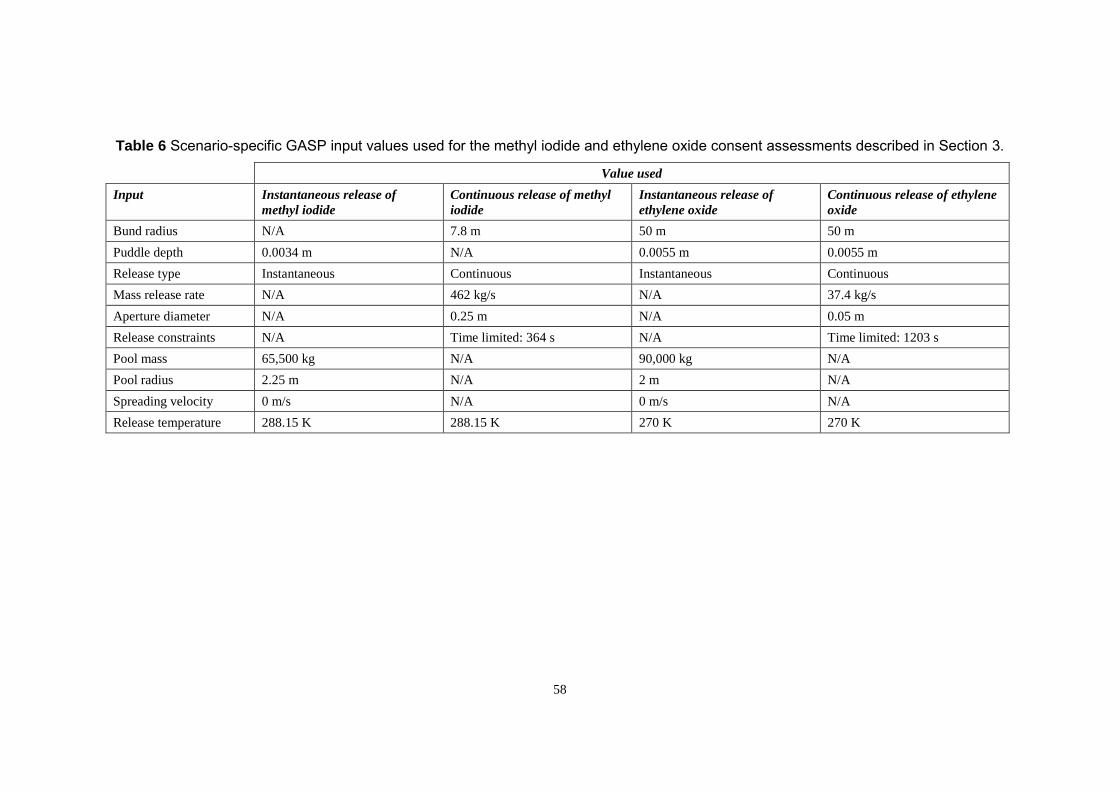
58
Table 6 Scenario-specific GASP input values used for the methyl iodide and ethylene oxide consent assessments described in Section 3.
Value used
Input Instantaneous release of
methyl iodide
Continuous release of methyl
iodide
Instantaneous release of
ethylene oxide
Continuous release of ethylene
oxide
Bund radius N/A 7.8 m 50 m 50 m
Puddle depth 0.0034 m N/A 0.0055 m 0.0055 m
Release type Instantaneous Continuous Instantaneous Continuous
Mass release rate N/A 462 kg/s N/A 37.4 kg/s
Aperture diameter N/A 0.25 m N/A 0.05 m
Release constraints N/A Time limited: 364 s N/A Time limited: 1203 s
Pool mass 65,500 kg N/A 90,000 kg N/A
Pool radius 2.25 m N/A 2 m N/A
Spreading velocity 0 m/s N/A 0 m/s N/A
Release temperature 288.15 K 288.15 K 270 K 270 K
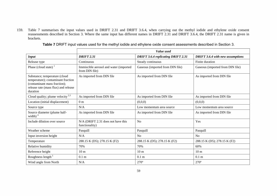
59
159. Table 7 summarises the input values used in DRIFT 2.31 and DRIFT 3.6.4, when carrying out the methyl iodide and ethylene oxide consent
reassessments described in Section 3. Where the same input has different names in DRIFT 2.31 and DRIFT 3.6.4, the DRIFT 2.31 name is given in
brackets.
Table 7 DRIFT input values used for the methyl iodide and ethylene oxide consent assessments described in Section 3.
Value used
Input DRIFT 2.31 DRIFT 3.6.4 replicating DRIFT 2.31 DRIFT 3.6.4 with new assumptions
Release type Continuous Steady continuous Finite duration
Phase (cloud state) 1 Immiscible aerosol and water (imported
from DIN file)
Gaseous (imported from DIN file) Gaseous (imported from DIN file)
Substance; temperature (cloud
temperature); contaminant fraction
(contaminant mass fraction);
release rate (mass flux) and release
duration
As imported from DIN file As imported from DIN file As imported from DIN file
Cloud quality; plume velocity 2,3
As imported from DIN file As imported from DIN file As imported from DIN file
Location (initial displacement) 0 m (0,0,0) (0,0,0)
Source type N/A Low momentum area source Low momentum area source
Source diameter (plume half-
width) 4
As imported from DIN file As imported from DIN file As imported from DIN file
Include dilution over source N/A (DRIFT 2.31 does not have this
functionality)
No Yes
Weather scheme Pasquill Pasquill Pasquill
Input inversion height N/A No No
Temperature 288.15 K (D5); 278.15 K (F2) 288.15 K (D5); 278.15 K (F2) 288.15 K (D5); 278.15 K (F2)
Relative humidity 70% 70% 60%
Reference height 10 m 10 m 10 m
Roughness length 5
0.1 m 0.1 m 0.1 m
Wind angle from North N/A 270º 270º
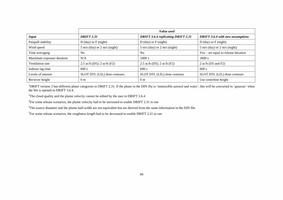
60
Value used
Input DRIFT 2.31 DRIFT 3.6.4 replicating DRIFT 2.31 DRIFT 3.6.4 with new assumptions
Pasquill stability D (day) or F (night) D (day) or F (night) D (day) or F (night)
Wind speed 5 m/s (day) or 2 m/s (night) 5 m/s (day) or 2 m/s (night) 5 m/s (day) or 2 m/s (night)
Time averaging No No Yes – set equal to release duration
Maximum exposure duration N/A 1800 s 1800 s
Ventilation rate 2.5 ac/h (D5); 2 ac/h (F2) 2.5 ac/h (D5); 2 ac/h (F2) 2 ac/h (D5 and F2)
Indoors lag time 600 s 600 s 600 s
Levels of interest SLOT DTL (LD1) dose contours SLOT DTL (LD1) dose contours SLOT DTL (LD1) dose contours
Receiver height 0 m 0 m Use centreline height
1DRIFT version 3 has different phase categories to DRIFT 2.31. If the phase in the DIN file is ‘immiscible aerosol and water’, this will be converted to ‘gaseous’ when
the file is opened in DRIFT 3.6.4.
2The cloud quality and the plume velocity cannot be edited by the user in DRIFT 3.6.4
3For some release scenarios, the plume velocity had to be increased to enable DRIFT 2.31 to run
4The source diameter and the plume half-width are not equivalent but are derived from the same information in the DIN file
5For some release scenarios, the roughness length had to be decreased to enable DRIFT 2.31 to run
61
7 REFERENCES
1. Webber DM, Jones SJ, Tickle GA, Wren T. A model of a dispersing dense gas cloud,
and the computer implementation DRIFT. I. Near-instantaneous releases. UKAEA
Report SRD/HSE R586, 1992.
2. Webber DM, Jones SJ, Tickle GA, Wren T. A model of a dispersing dense gas cloud,
and the computer implementation DRIFT. II. Steady continuous releases. UKAEA
Report SRD/HSE R587, 1992.
3. The Planning (Hazardous Substances) (Amendment) (England) Regulations 2009.
http://www.legislation.gov.uk/uksi/2009/1901/body/made (accessed March 2017).
4. Hazardous Substances. https://www.gov.uk/guidance/hazardous-substances (accessed
March 2017).
5. HSE’s land use planning methodology.
http://www.hse.gov.uk/landuseplanning/methodology.pdf (accessed March 2017).
6. Tickle GA, Carlisle JE. DRIFT Version 3.6: Mathematical model, Issue 5. ESR
Technology report, 2012.
7. Tickle GA, Carlisle JE. Extension of the dense gas dispersion model DRIFT to include
buoyant lift-off and buoyant rise. HSE Research Report RR629, 2008. Available from
http://www.hse.gov.uk/research/rrhtm/rr629.htm (accessed March 2017).
8. Tickle GA, Martin D, Ramsdale SA. EJECT – An integral model of a two-phase jet in a
cross-flow. AEA Technology Report AEAT-1517 Issue 2, 1998.
9. Macbeth R. The derivation of the physical properties of hazardous substances for
Substance Property Information (SPI) data files. HSL Report RAS/04/05, 2004.
10. Walton E. DRIFT COM Interface Guide, Issue 5. ESR Technology Limited report
ESR/D1000846/SUG02, 2011.
11. Tickle GA. Comparison of DRIFT Version 3 predictions with DRIFT Version 2 and
experimental data. ESR Technology report ESR/D1000846/STR01/Issue 3, 2012.
12. Tickle G, Godaliyadde D, Carlisle J. Comparisons of predictions from the gas
dispersion model DRIFT (Version 3) against URAHFREP data. ESR Technology report
ESR/D1000976/001/Issue 4, 2012. To be published in the HSE Research Report series
at http://www.hse.gov.uk/research/rrhtm/
13. Coldrick S, Webber D. Evaluation of the DRIFT gas dispersion model version 3.6.4.
HSE Research Report RR1100, 2017.
Available from http://www.hse.gov.uk/research/rrhtm/rr1100.htm (accessed March
2017).
14. Ivings MJ, Jagger SF, Lea CJ, Webber DM. Evaluating Vapor Dispersion Models for
Safety Analysis of LNG Facilities. Fire Protection Research Foundation, National Fire
Protection Association, April 2007. Available from www.nfpa.org
62
15. Toxicity levels of chemicals. http://www.hse.gov.uk/chemicals/haztox.htm (accessed
March 2017).
16. DRIFT Version 3 user guide, Issue 5. ESR Technology report, 2011.
17. Webber DM. A model for pool spreading and vaporisation and its implementation in
the computer code GASP. SRD/HSE R507, ISBN 0-853563519, September 1990.
18. Britter RE, McQuaid J. Workbook on the dispersion of dense gases. HSE Contract
Research Report 17/1988, 1988.
Available from http://www.hse.gov.uk/research/crr_pdf/1988/crr88017.pdf (accessed
March 2017).
19. Characteristics of wind speed in the lowest layers of the atmosphere near the ground:
Strong winds. ESDU 72026, Engineering Sciences Data Unit Ltd., 1972.
20. Smedman-Högström A-S, Högström U. A practical method for determining wind
frequency distributions for the lowest 200 m from routine meteorological data. J. Appl.
Meteorol. 17 (1972) 942.
21. van den Bosch CJH, Weterings RAPM (ed). Methods for the calculation of physical
effects due to releases of hazardous materials (liquids and gases) ‘Yellow Book’. CPR
14E, TNO (The Netherlands Organization of Applied Scientific Research), Third
edition, Second revised print, 2005.
22. Hanna SR, Britter RE. Wind flow and vapor cloud dispersion at industrial and urban
sites. CCPS (Center for Chemical Process Safety), AIChE (American Institute of
Chemical Engineers), ISBN: 978-0-8169-0863-9, 2002.
23. Nielsen M, Chatwin PC, Jorgensen HE, Mole N, Munro RJ, Ott S. Concentration
fluctuations in gas releases by industrial accidents. Technical Report Risø-R-1329(EN),
Risø National Laboratory, May 2002.
24. Wheatley CJ. Dispersion of a passive puff released at the ground into the diabatic
atmospheric boundary layer. Technical Report SRD/HSE R445, UKAEA, August
1988.
25. Tickle GA. Model predictions compared with URAHFREP campaign 2 field trial data.
Technical Report AEAT/NOIL/27328006/003 (R) Issue 2, AEA Technology, June
2001. A deliverable produced under work package 7 of the EC URAHFREP project,
Contract No. ENV4-CT97-0630.
26. Hurst NW, Nussey C, Pape RP. Development and application of a risk assessment tool
(RISKAT) in the Health and Safety Executive. Chem. Eng. Res. Des. 67(4) (1989) 362.
27. Davies PC, Purdy G. Toxic gas risk assessments – the effect of being indoors.
Refinement of Estimates of the Consequences of Heavy Toxic Vapour Releases.
IChemE Symposium No 1, Manchester, January 1986.
28. Lines IG, Daycock JH, Deaves DM. Guidelines for the inclusion of low wind speed
conditions into risk assessments. HSE Contract Research Report 276/2000, 2000.
Available from http://www.hse.gov.uk/research/crr_pdf/2000/crr00276.pdf (accessed
March 2017).

63
29. Serghides TK. Estimate friction factor accurately. Chem. Eng. J. 91(5) (1984) 63.
30. Brighton PWM. Evaporation from a plane liquid surface into a turbulent boundary
layer. SRD/HSE R375, ISBN: 0-85-356-223-7, January 1987.

64

Published by the Health & Safety Executive 08/17
Modelling the dispersion of vapour from pools of toxic liquids using DRIFT 3
RR1101
www.hse.gov.uk
The Health and Safety Executive (HSE) uses gas dispersion modelling in its assessment of the hazards and risks posed by toxic and flammable substances stored at major hazards sites. To update its dispersion modelling capability, HSE recently commissioned ESR Technology to develop a new version of the gas dispersion model DRIFT (Dispersion of Releases Involving Flammables or Toxics). The new version of the model, DRIFT 3, includes a significant number of modelling enhancements over the version of DRIFT previously used within HSE (DRIFT 2.31). These include the extension of the model to treat buoyant plumes and time varying releases. Prior to DRIFT 3 being adopted for use by HSE, it must undergo thorough evaluation and assessment for a range of release scenarios.
This report considers the dispersion of vapour from pools of toxic liquids, such as methyl iodide and ethylene oxide, and presents an assessment of the performance of DRIFT 3.6.4 for modelling such release scenarios. Sensitivity tests have shown that DRIFT 3.6.4 works reliably for the types of toxic pool scenario typically used by HSE to assess Hazardous Substances Consent applications and set Land Use Planning zones around major hazards sites.
As a result of this work and accompanying evaluation studies (see Research Report RR1100), DRIFT 3.6.4 has been adopted by HSE to model the dispersion of vapour evolved from pools of toxic liquids.
This report and the work it describes were funded by the Health and Safety Executive (HSE). Its contents, including any opinions and/or conclusions expressed, are those of the authors alone and do not necessarily reflect HSE policy.


