Poroelastic modeling of seismic boundary conditions acrossa fracturea)

Seiji Nakagawab�

Earth Sciences Division, Lawrence Berkeley National Laboratory, 1 Cyclotron Road, Berkeley,California 94720

Michael A. Schoenberg5 Mountain Road, West Redding, Connecticut 06896

�Received 19 December 2006; revised 15 May 2007; accepted 16 May 2007�

Permeability of a fracture can affect how the fracture interacts with seismic waves. To examine thiseffect, a simple mathematical model that describes the poroelastic nature of wave-fractureinteraction is useful. In this paper, a set of boundary conditions is presented which relatewave-induced particle velocity �or displacement� and stress including fluid pressure across acompliant, fluid-bearing fracture. These conditions are derived by modeling a fracture as a thinporous layer with increased compliance and finite permeability. Assuming a small layer thickness,the boundary conditions can be derived by integrating the governing equations of poroelastic wavepropagation. A finite jump in the stress and velocity across a fracture is expressed as a function ofthe stress and velocity at the boundaries. Further simplification for a thin fracture yields a set ofcharacteristic parameters that control the seismic response of single fractures with a wide range ofmechanical and hydraulic properties. These boundary conditions have potential applications insimplifying numerical models such as finite-difference and finite-element methods to computeseismic wave scattering off nonplanar �e.g., curved and intersecting� fractures.�DOI: 10.1121/1.2747206�

PACS number�s�: 43.40.Ph, 43.20.Gp, 43.20.Bi �LLT� Pages: 831–847

I. INTRODUCTION

Rock is often permeated by compliant plane discontinui-ties �such as fractures and faults� that, depending on theirpermeability relative to the background, serve as either con-duits or barriers to subsurface fluid flow �e.g., Aydin, 1978;Adams and Dart, 1998�. In the following, we shall collec-tively call these discontinuities “fractures.” The fluid perme-ability of a fracture is often a key parameter, yet the quanti-tative relationship between permeability and its effect onseismic wave scattering is not fully understood. Strong scat-tering of seismic waves by a fracture is usually related tolarge permeability, because an open fracture with partial sur-face contacts has increased mechanical compliance �deform-ability� �e.g., Pyrak-Nolte and Morris, 2001�. However, if afluid-containing fracture is filled with debris, or a single frac-ture consists of a large number of microcracks, complex in-teractions between rock and pore fluid in the fracture result.In this paper, we will develop a simple mathematical modelthat captures the essential nature of solid-fluid interactionwithin a fracture, to predict the effect of hydraulic permeabil-ity and other fracture properties on seismic wave scattering.

One logical tool for probing the hydrological propertiesof rocks using seismic waves is Biot’s theory of poroelastic-ity �Biot, 1956a, b�, which describes the dynamic interac-

a�Portions of this work were presented in “Poroelastic modeling of seismicboundary conditions across a fracture,” Expanded abstract for the annualmeeting for the Society of Exploration Geophysicists, New Orleans, 1–5Oct. 2006.

b�

Electronic mail: snakagawa@lbl.gov

J. Acoust. Soc. Am. 122 �2�, August 2007 0001-4966/2007/122�2

tions of rock and fluid within the pore space. It has beenwidely recognized, however, that the dispersion and attenu-ation of seismic waves predicted by the original Biot’stheory—which applies to macroscopically homogeneous po-rous media saturated by a single fluid phase—is often toosmall to explain the measured velocity dispersion and attenu-ation of seismic waves. In recent decades, many researchersrealized that significant velocity dispersion and velocity at-tenuation can result at field-relevant frequencies if a rockcontains heterogeneity at mesoscale �smaller than seismicwavelength but larger than pore and grain size�. One sucheffect is due to a local fluid-pressure gradient induced atscales comparable to the pressure diffusion length �or, wave-length of Biot’s slow compressional waves�. These heteroge-neities can be, for example, a “patchy” distribution of fluidand gas within rocks �e.g., White, 1975; Dutta and Odé,1979a, b; and Johnson, 2001� and stratified sedimentary unitswith different mechanical and hydrological properties �Nor-ris, 1993; Gurevich et al., 1994, 1997; Gelinsky and Shapiro,1997; Shapiro and Müller, 1999; Pride et al., 2002�. A moregeneral theory for heterogeneous poroelastic media, with ar-bitrary distributions of mechanical and hydraulic propertiesfor both solid and fluid phases, was recently developed byPride and Berryman �2003a, b�.

In general, within porous fluid-bearing rocks, the stron-ger the fluid permeability and mechanical-property heteroge-neity, the more the velocity and attenuation of seismic wavesare affected. Fractures are a special case of such heterogene-

ity, exhibiting an extremely wide range of mechanical com-

831�/831/17/$23.00

pliance and hydraulic permeability �for example, open, air-filled joints to near-rigid, mineral-filled veins�, even thoughthey typically occupy only a small volume. Berryman andWang �1995� examined the mechanical consolidation of me-dia containing a system of compliant high-permeability frac-tures within a porous background medium, and then used thederived elastic moduli to examine the velocity dispersion andattenuation of low-frequency seismic waves �Berryman andWang, 2000�. The results indicated that the mechanical andhydraulic properties of fractures in a porous host rock affectthe behavior of seismic waves. For one-dimensional P-wavepropagation within a medium containing parallel periodicfractures, Brajanovski et al. �2005� derived an analyticalmodel for the dispersion and attenuation of waves. Thismodel was derived by using a wave propagation model foralternating poroelastic layers developed by Norris �1993� andtaking the zero-thickness limit of one of the constituting lay-ers to model fractures. Through numerical experiments, at-tenuation and dispersion of P wave propagation was found tobe strongly dependent upon the fracture properties �fracturestiffness and density� and the background porosity.

In contrast to previous research, which focused on thevelocity and attenuation of waves propagating through mate-rials containing many fractures, in this paper we will developa simple mathematical model for single poroelastic fracturesthat can be used to study discrete scattering of seismicwaves. The model consists of a set of boundary conditionsthat relate the stress and displacement �or particle velocity�induced on the fracture surface by passing seismic waves.These boundary conditions are derived using plane-wavetheory, by treating a fracture as a thin poroelastic layer withan infinite extent and a small finite thickness. Alternatively,scattering of the plane waves can be examined by using apropagator-matrix method �e.g., Haskell, 1953� and Ken-nett’s reflectivity method �Kennett, 1983� to find an exactrelationship between the amplitude of incident and scatteredwaves. However, the propagator-matrix method suffers aninstability when the Biot’s slow P wave decays too quickly;and Kennett’s method results in very complex expressions ofthe boundary conditions that are not amenable to simple pa-rametrization and interpretation of the consequences forphysical acoustics. Further, because both of these methodsrequire knowledge of incident plane waves on both sides of afracture, they are not well suited to use in other numericalmodels, such as finite-difference and finite-element methods.

The model developed in this paper provides “jump con-ditions” that directly relate a wave’s particle motions andstress across a fracture without the knowledge of the wavefield in the background. Such boundary conditions were ini-tially developed for elastic and viscoelastic fractures, andcalled the “linear-slip interface model” �Schoenberg, 1980�,which led to a plethora of theories and models describing thecomplex interaction between seismic waves and fractures—e.g., plane-wave scattering theories by Schoenberg �1980�,Nakagawa et al. �2000�, laboratory experiments by Pyrak-Nolte et al. �1990�, Hsu and Schoenberg �1993�, fracture-based anisotropic effective medium theories of Schoenbergand Sayers �1999�, Bakulin et al. �2000�, fracture guided

wave studies by Pyrak-Nolte and Cook �1987�, and Nihei et

832 J. Acoust. Soc. Am., Vol. 122, No. 2, August 2007 Nakagawa

al. �1999�. More recently, Bakulin and Molotkov �1997� de-veloped a similar model for poroelastic fractures, but withoutincluding the effect of fracture permeability. These modelscan be very simple, because when the relative thickness of afracture is much smaller than the seismic wavelengths �Bi-ot’s fast P waves and S waves�, and inertia-related quantities�given as a product of density and fracture thickness� can beignored, only quasistatic behavior needs to be described�Rokhlin and Wang, 1991�. Gurevich et al. �1994� also usedthis fact to derive simple, computationally stable expressionsdescribing the transmission and reflection coefficients of nor-mally incident fast P waves for a thin poroelastic layer. Be-cause of its simplicity, the linear-slip model can be used infinite-difference codes to determine the proper effectiveanisotropic-elastic-moduli values of the numerical grids on afracture, when the thickness of the fracture is much smallerthan the modeling grid spacing �Coates and Schoenberg,1995�.

One important aspect of the linear-slip interface modelis that it helps to identify important characteristic parametersof a fracture that control the scattering of seismic waves. Anexample of such parameters is the fracture compliance. If afracture is modeled as a mechanically equivalent, thin, com-pliant layer with a finite thickness, the fracture compliancecan be defined as an inverse of the elastic moduli times frac-ture thickness �e.g., Rokhlin and Wang �1990� defined a frac-ture stiffness parameter �inverse of the fracture compliance�in this way�. Coates and Schoenberg �1995� developed afinite-difference model for fractures and faults, based uponthe finite-thickness approximation of fractures and faults.Conversely, when physical properties of a fracture are to bedetermined using seismic waves, what we can at best deter-mine are these “phenomenological” model parameters �in-stead of the original material properties and fracture thick-ness�. For a fracture viewed as a thin poroelastic layer, wewill show that characteristic parameters similar to the origi-nal linear-slip interface model can be defined for a poroelas-tic fracture, along with other dimensionless parameters thatdescribe its poroelastic properties.

In the following, first we will derive poroelastic seismicboundary conditions �linear-slip interface model� based uponthe governing equations of linear, poroelastic wave propaga-tion �Secs. II A and II B�. This will result in two sets ofindependent matrix equations relating displacement andstress across a fracture, which are the primary results of thiswork. The critical step in this derivation is an approximationof the wave-induced pressure field within a fracture—this isnecessary because the exact pressure distribution cannot bedetermined only from the boundary values. Subsequently, as-suming a fracture thickness much smaller than the wave-length of propagating body waves, the derived boundaryconditions will be simplified to obtain the characteristic frac-ture parameters �Sec. II C�. The original and simplifiedboundary conditions will be used to derive explicit expres-sions for plane-wave transmission and reflection coefficients�Sec. II D�. Sections III A and III B will examine the accu-racy of the derived boundary conditions �both original andsimplified� by comparing the predicted transmission and re-

flection coefficients to the exact results obtained via Ken-

and Schoenberg: Poroelastic boundary conditions across a fracture

nett’s reflectivity method. Finally, the sensitivity of the trans-mission and reflection coefficients to the permeability of afracture will be examined using a characteristic fracture pa-rameter �Sec. III C�.

II. THEORY

In this section, we will derive a set of boundary condi-tions for a thin, isotropic, homogeneous, poroelastic layerembedded within a background medium. �A derivation ofboundary conditions assuming a transversely isotropic po-roelastic layer for a fracture is also presented in AppendixA.� Subsequently, these boundary conditions are used to de-rive expressions for transmission and reflection coefficientsof incident plane waves within a poroelastic background me-dium.

A. Governing equations

The governing equations of seismic wave propagationwithin an isotropic, homogeneous, poroelastic medium canbe stated as �e.g., Pride et al., 2002�

� = G��u + u � � + ��KU − 2G/3� � · u + C � · w�I , �1�

− pf = C � · u + M � · w , �2�

� · � = − �2��u + � fw� , �3�

− �pf = − �2�� fu + �w�, � � i� f/�k��� , �4�

where u is the locally averaged, solid-frame displacementvector and w���U-u� is the fluid-volume displacement vec-tor relative to the solid frame. In this definition of w, U is thelocally averaged �in the pore space� fluid displacement vec-tor and � is the porosity. Equations �1�–�4� assume that thedisplacement and stress variables depend on exp�−i�t�,where � is the circular frequency. I indicates an identitytensor, � is the total stress tensor, and pf is the fluid pressure�positive for compression�. G is the solid-frame shear modu-lus, KU is the undrained bulk modulus, � is the bulk density,� f is the fluid modulus, and the parameter � is defined in Eq.�4� via fluid viscosity � f and the frequency-dependent per-meability k��� �Johnson et al., 1987�. C and M are the Biot’scoupling and fluid-storage moduli, respectively. When aplane harmonic wave field is assumed, these equations resultin the four plane-wave modes of a Biot medium �fast andslow P waves and two S waves�.

Consider an interface across which certain stress and

displacement �velocity� components are conserved. We as-

J. Acoust. Soc. Am., Vol. 122, No. 2, August 2007 Nakagawa and Sc

sume this interface to be normal to the 3 direction of Carte-sian coordinates, and wave propagation parallel to the 1, 3plane �Fig. 1�. For a homogeneous medium, we can assume aplane harmonic wave field proportional to exp i���1x1− t�,where �1 is the slowness in the 1 direction. The plane-wavedisplacement and stress are introduced into Eqs. �1�–�4�.Substituting � /�x1→ i��1 and � /�x2→0 and eliminatingcomponents of the vector and tensor variables w1, w2, �11,�22, and �12 �which can be discontinuous across the inter-face�, the following two independent sets of coupled first-order differential equations are derived:

�

�x3� u2

�23� = − i�� 0 1/G

− G�12 + ��� − � f

2�/� 0�� u2

�23� �

− i�R� u2

�23� , �5�

�

�x3�u1

�33

− pf

�13

u3

w3

= − i�� 0 QXY

QYX 0��

u1

�33

− pf

�13

u3

w3

, �6�

where

QXY � �1/G �1 0

�1 � � f

0 ˜ , �7�

FIG. 1. Cartesian coordinate system used in this paper.

� f �

QYX � �− 4G�1

21 −G

HD� −

� f2 − ��

��11 −

2G

HD� �1−

� f

�+ �

2G

HD�

�11 −2G

HD� 1

HD−

�

HD

�1−� f

�+ �

2G

HD� −

�

HD

�2

HD+

1

M−

�12

�

. �8�

hoenberg: Poroelastic boundary conditions across a fracture 833

Equation �5� is for wave propagation of S waves with par-ticle motions in the 2 direction, and Eq. �6� is for coupled P�both fast and slow�-S wave propagation with particle mo-tions within the 1,3 plane. Note that both �R��1 ,�� � =0 and�QXY��1 ,�� � =0 yield the dispersion equation for S waves,and �QYX��1 ,�� � =0 results in the dispersion equation for fastand slow P waves, where � · � indicates the matrix determi-nant. The dots over the displacement vector components inEqs. �5� and �6� indicate that the related quantity is velocity.In Eqs. �7� and �8�, HD�KD+4G /3 is the dry P-wave modu-lus and �= �1−KD /KU� /B is the Biot-Willis effective stresscoefficient �with B as the Skempton coefficient�. Using thesecoefficients, C and M in the governing equations can beexpressed as C=BKU and M =BKU /�. Further, if grains inthe porous rock are both isotropic and homogeneous,

� = 1 − KD/Ks, �9�

B =1/KD − 1/Ks

�1/KD − 1/Ks� + ��1/Kf − 1/Ks�, �10�

where KD is the dry bulk modulus, Ks is the solid �grain�bulk modulus, Kf is the fluid bulk modulus, and � is theporosity of the medium.

B. Derivation of poroelastic boundary conditions fora fracture

The boundary conditions for a poroelastic fracture areobtained by integrating the governing equations in Eqs. �5�and �6� over a small layer or fracture thickness h as

� u2+ − u2

−

�23+ − �23

− � = − i�h� 0 1/G

− G�12 + ��� − � f

2�/� 0�� u2

�23� ,

�11�

�u1

+ − u1−

�33+ − �33

−

− pf+ − �− pf

−��13

+ − �13−

u3+ − u3

−

w3+ − w3

−

= − i�h� 0 QXY

QYX 0��

u1

�33

− pf

�13

u3

w3

, �12�

where the superscripts + and − indicate quantities on theboundaries, and the bars above the variables indicate aver-aged quantities over the thickness of the fracture. At thispoint, Eqs. �11� and �12� are without approximations, exceptthat we assumed homogeneity of the medium and plane-wave propagation. To derive boundary conditions, the aver-aged quantities on the right-hand side of the equations haveto be expressed exclusively using quantities on the bound-aries.

Since the thickness of a fracture h is usually muchsmaller than seismic wavelengths, the inertial effect andcomplex multiple scattering of the waves within the fracture

can be ignored. This allows us to assume that the solid-frame

834 J. Acoust. Soc. Am., Vol. 122, No. 2, August 2007 Nakagawa

velocity and the total stress within the fracture varysmoothly, which can be approximated by a linear function.Also, since the field distribution must be defined by twoboundary values on the fracture surfaces, and since there isno knowledge of the field’s functional form, a linear functionprovides the best guess. For Eq. �11�, therefore, the boundarycondition becomes

� u2+ − u2

−

�23+ − �23

− � = −i�h

2� 0 1/G

− G�12 + ��� − � f

2�/� 0�

�� u2+ + u2

−

�23+ + �23

− � . �13�

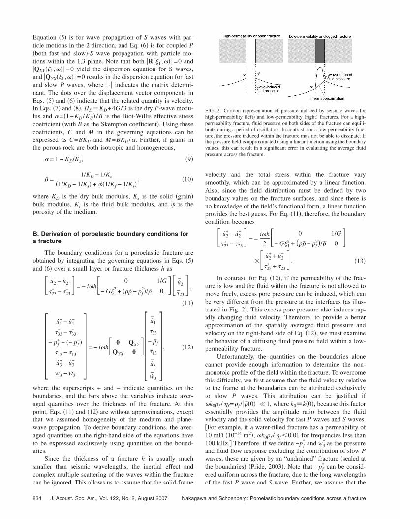
In contrast, for Eq. �12�, if the permeability of the frac-ture is low and the fluid within the fracture is not allowed tomove freely, excess pore pressure can be induced, which canbe very different from the pressure at the interfaces �as illus-trated in Fig. 2�. This excess pore pressure also induces rap-idly changing fluid velocity. Therefore, to provide a betterapproximation of the spatially averaged fluid pressure andvelocity on the right-hand side of Eq. �12�, we must examinethe behavior of a diffusing fluid pressure field within a low-permeability fracture.

Unfortunately, the quantities on the boundaries alonecannot provide enough information to determine the non-monotoic profile of the field within the fracture. To overcomethis difficulty, we first assume that the fluid velocity relativeto the frame at the boundaries can be attributed exclusivelyto slow P waves. This attribution can be justified if�k0� f /� f =� f / ���0� � �1, where k0�k�0�, because this factoressentially provides the amplitude ratio between the fluidvelocity and the solid velocity for fast P waves and S waves.�For example, if a water-filled fracture has a permeability of10 mD �10−14 m2�, �k0� f /� f 0.01 for frequencies less than100 kHz.� Therefore, if we define −pf

* and w3* as the pressure

and fluid flow response excluding the contribution of slow Pwaves, these are given by an “undrained” fracture �sealed atthe boundaries� �Pride, 2003�. Note that −pf

* can be consid-ered uniform across the fracture, due to the long wavelengths

FIG. 2. Cartoon representation of pressure induced by seismic waves forhigh-permeability �left� and low-permeability �right� fractures. For a high-permeability fracture, fluid pressure on both sides of the fracture can equili-brate during a period of oscillation. In contrast, for a low-permeability frac-ture, the pressure induced within the fracture may not be able to dissipate. Ifthe pressure field is approximated using a linear function using the boundaryvalues, this can result in a significant error in evaluating the average fluidpressure across the fracture.

of the fast P wave and S wave. Further, we assume that the

and Schoenberg: Poroelastic boundary conditions across a fracture

spatial average of u1 and �33 for this field can be approxi-mated by the average of the total field u1 and �33. This as-sumption can be justified if the incident wave is not a slow Pwave and the frequency is low, which results in amplitudesof scattered slow P waves much smaller than the sum of theother waves.

Under these assumptions, the jump condition for fluidvelocity in the matrix equation �the bottom row of Eq. �12��can be used to obtain the following relationship:

w3+* − w3

−* = 0 = − i�h��1−� f

�+ 2�

G

HD�u1 −

�

HD�33

+ �2

HD+

1

M−

�12

���− pf

*�� . �14�

The fluid velocity within the undrained fracture is w3*=0.

From the above equation,

− pf* = �1

� f

�− 2�

G

HD

�2

HD+

1

M−

�12

�

u1 +

�

HD

�2

HD+

1

M−

�12

�

�33 �

− 2GB�1u1 + B�33, �15�

where we introduced the following coefficients B and forconvenience:

1

B� � +

HD

�M−

�12

�

HD

�=

HU

�M−

�12

�

HD

�, �16�

� 1 −HD

2�G

� f

�. �17�

The first term on the right-hand side of Eq. �15� indicates acontribution of the strain induced in the fracture-parallel di-rection �−�1u1=�u1 /�x1�.

Next, we derive an expression for the diffusing pressureand flow field within a fracture using the pressure and veloc-ity at the boundaries and the pressure and velocity for theundrained condition. The solution of diffusing field for slowwaves with a slowness �Ps is expressed as

f�x3� = A1ei��Psx3 + A2e−i��Psx3. �18�

We assume that the direction of the diffusion is in the plane-normal direction, which is a reasonable assumption if thevelocity of the incoming wave is much faster than the slowP-wave velocity within the fracture. For a set of boundaryconditions f�0�=0 and f�h�=1, the two unknown coefficientsare determined, resulting in

f�x3� =ei��Psx3 − e−i��Psx3

ei��Psh − e−i��Psh. �19�

When integrated over an interval �0, h�, Eq. �19� becomes

0

h

f�x3�dx3 =h

2·

tan ��Psh/2

��Psh/2�

h

2���� , �20�

where we defined the following dimensionless function:

J. Acoust. Soc. Am., Vol. 122, No. 2, August 2007 Nakagawa and Sc

���� �tanh �

�, � � −

i��Psh

2=

h

2 d* . �21�

The complex fluid-pressure diffusion length d* is defined

through i��Ps�−1/ d*. We shall call the dimensionless func-

tion � �Fig. 3� a “fluid-pressure dissipation factor,” whichapproaches unity for the low-frequency limit �drained re-sponse� and approaches zero for the high-frequency limit�undrained response�. For the aforementioned low frequen-cies and low-permeability conditions satisfying�� fk0 /� f�1, the following simple relationship can be usedto compute d

* �e.g., Pride, 2003�:

1

* =1 − i

d, �22�

FIG. 3. �Color online� Fluid pressure dissipation factor � as a function ofthe dimensionless length parameter h /2 d. The behavior of the functionchanges when the diffusion length is half of the layer thickness, separatingthe low-frequency drained response �left-hand side of the h /2 d�1� and thehigh-frequency undrained response �right-hand side�. �a� Amplitude; �b�Phase �Asymptotes to � /4 for the undrained response�.

d

hoenberg: Poroelastic boundary conditions across a fracture 835

d =�2D

�, �23�

D =k0M

� f1 −

C2

HUM� =

k0M

� f1 −

�2M

HU� , �24�

where d is the fluid-pressure diffusion length and D is thefluid-pressure diffusion coefficient. Using the solution forf�x3�, the pressure and fluid velocity within a fracture isgiven by a superposition having the boundary conditions−pf�x3=0�=−pf

−, −pf�x3=h�=−pf+, and w3�x3=0�= w3

−,w3�x3=h�= w3

+. These are

pf�x3� = pf* − �pf

* − pf+�f�x3� − �pf

* − pf−�f�h − x3� , �25�

w3�x3� = w3* − �w3

* − w3+�f�x3� − �w3

* − w3−�f�h − x3�

= w3+f�x3� + w3

−f�h − x3� . �26�

As an example, pressure amplitude profiles are shown belowin Fig. 4 for assumed boundary values of −pf

−=0.25, −pf+

=0.75, and −pf*=1. As seen from the plot, the transition be-

tween the drained response �linear pressure profile� and theundrained response �constant pressure within the fracture�occurs approximately when h /2 d=1, i.e., the sum of thewavelength for the two diffusing pressure waves equals thethickness of the fracture.

Using the result in Eq. �20�, pressure and fluid velocity

averaged across a fracture is

836 J. Acoust. Soc. Am., Vol. 122, No. 2, August 2007 Nakagawa

pf =1

h

0

h

pf�x3�dx3 = pf* − �2pf

* − pf− − pf

+�1

2· ����

=pf

− + pf+

2· ���� + pf

* · �1 − ����� , �27�

w =1

h

0

h

w3�x3�dx3 =w3

− + w3+

2���� . �28�

Equations �15�, �27�, and �28� are introduced within the ma-

FIG. 4. Amplitude profiles of the pressure field within a fracture for a rangeof diffusion lengths d. For very large d’s �i.e., high frequency, low perme-ability�, the pressure within the fracture can take a value independent fromthe pressure on the fracture surfaces.

trix boundary conditions in Eq. �12� to yield

�u1

+ − u1−

�33+ − �33

−

− pf+ − �− pf

−��13

+ − �13−

u3+ − u3

−

w3+ − w3

−

= − i�h� 0 QXY

QYX 0��

u1+ + u1

−

2

�33+ + �33

−

2

− pf− + �− pf

+�2

· � + B �33+ + �33

−

2− 2G�1

u1+ + u1

−

2� · �1 − ��

�13+ + �13

−

2

u3+ + u3

−

2

w3− + w3

+

2· �

. �29�

The solid displacement �or velocity� u1, u3 and total stress �13, �33 are assumed to vary linearly, because the field changesslowly within the fracture. The above equation is recast in the following form:

and Schoenberg: Poroelastic boundary conditions across a fracture

�u1

+ − u1−

�33+ − �33

−

− pf+ − �− pf

−��13

+ − �13−

u3+ − u3

−

w3+ − w3

−

= −i�h

2 � 0 QXY

QYX 0��

u1+ + u1

−

�33+ + �33

−

− pf+ + �− pf

−��13

+ + �13−

u3+ + u3

−

w3+ + w3

−

,

�30�

where

QXY = QXY�1 0 0

0 1 0

0 0 � = �1/G �1 0

�1 � � f · �

0 � f � · � , �31�

QYX = QYX� 1 0 0

0 1 0

− 2GB�1 · �1 − �� B · �1 − �� � . �32�

The components of the matrix QYX are given explicitly as

QYX�1,1� = − 4G�121 −

G

HD� −

� f2 − ��

�

− 2GB�12−

� f

�+ �

2G

HD� · �1 − �� , �33�

QYX�1,2� = �1�1 −2G

HD� + −

� f

�+ �

2G

HD�B · �1 − ��� ,

�34�

QYX�1,3� = �1−� f

�+ �

2G

HD� · � , �35�

QYX�2,1� = �11 −2G

HD+ 2B�

G

HD· �1 − ��� , �36�

QYX�2,2� =1

HD− �B

1

HD· �1 − �� , �37�

QYX�2,3� = − �1

HD· � , �38�

QYX�3,1� = �1�−� f

�+ �

2G

HD− 2B�2 G

HD+

G

M

−�1

2G

�� · �1 − ��� , �39�

QYX�3,2� = − �1

HD+ �2 1

HD+

1

M−

�12

��B · �1 − �� ,

�40�

J. Acoust. Soc. Am., Vol. 122, No. 2, August 2007 Nakagawa and Sc

QYX�3,3� = �2 1

HD+

1

M−

�12

�� · � . �41�

Together, Eqs. �13� and �30� are the seismic boundary con-ditions for a poroelastic fracture.

C. Simplified boundary conditions and characteristicparameters of a fracture

Mathematically, if the components of the matrices inEqs. �13� and �30� remain finite when the fracture thicknessis reduced to zero, the right-hand side of the equations van-ishes, and all the variables are continuous across the fracture.However, in reality, a very thin fracture can produce a largediscontinuity in displacement and pressure field if viewed asa boundary. For our model to properly capture this behavior,the material properties of a fracture contained in the matrixboundary conditions in Eqs. �13� and �30� have to take val-ues that result in significantly large matrix components, evenwhen multiplied by the small fracture thickness h. To dealwith this situation, we can define composite characteristicparameters of a fracture as a combination of the materialproperties and the fracture thickness, which control the dy-namic behavior of the fracture. Conversely, when physicalproperties of a fracture are to be determined using seismicwaves without the knowledge of the fracture thickness, atbest we can determine these composite or “phenomenologi-cal” parameters instead of the original material properties,such as bulk permeability and elastic moduli.

From Eqs. �13� and �30�, following parameters involvingfracture thickness h may be defined:

�T �h

G�shear compliance� , �42�

�ND�

h

HD�dry or drained normal compliance� , �43�

���� �k���

h�membrane permeability� . �44�

If we assume that these parameters are finite for small frac-ture thicknesses h’s, approximate boundary conditions can beobtained by replacing the moduli and permeability in theequations by the parameters and eliminating O�h� terms. ForSh waves, this reduces the coefficient matrix in Eq. �13� to

h � � 0 1/G

− G�12 + ��� − � f

2�/� 0� → �T�0 1

0 0� . �45�

Therefore, the boundary conditions are

�u2+ − u2

− = �− i���T�23−

�23+ = �23

− , �46�

which are exactly the same as the original linear-slip inter-face model �Schoenberg, 1980�.

For the two coupled matrix boundary conditions in Eq.�30� for fast and slow P waves and an S wave, the coefficient

matrices QXY and QXY in Eqs. �31� and �32�, multiplied by h,

respectively, reduce to

hoenberg: Poroelastic boundary conditions across a fracture 837

h � QXY → ��T 0 0

0 0 0

0 0 i� f/����� · � , �47�

h � QYX → �ND�0 0 0

0 1 − �B�1 − �� − � · �

0 − � · � �/B · � , �48�

where we used �1, which resulted from Eq. �17� throughO�h�→0. The Skempton coefficient-like parameter in Eq.�16� also reduces to

B � �M

HU. �49�

Compared to the original Skempton coefficient B, this newcoefficient is defined with the undrained P-wave modulusHU rather than the bulk modulus KU. Furthermore, the fluid

pressure dissipation factor ���� is simplified by approximat-

to be transversely isotropic, however, the two compliance

838 J. Acoust. Soc. Am., Vol. 122, No. 2, August 2007 Nakagawa

ing the complex diffusion coefficient in Eq. �24� as

D �k0M

� f1 −

C2

HUM� =

k0

� f

MHD

HU=

B�0

�� f�ND

h2, �50�

which results in

� =h

2 d* =

h

2�1 − i�� �

2D=

1 − i

2��

�� f�ND

2B�0

. �51�

Therefore, for a set of characteristic fracture parameters,���� also does not depend on the fracture thickness. Notethat in deriving Eq. �48�, the matrix components in Eqs.�33�–�41� containing h / �=�k���h / i� f were ignored, evenfor fractures with very high �static� permeability. This is be-cause the dynamic permeability of a fracture is finite evenwhen the static permeability of the material within the frac-ture approaches infinity, which results in an explicit bound�h / � � �h /� f �Appendix B�.

Using the simplified relationships in Eqs. �47�–�51�, the

boundary conditions are written explicitly as

�u1

+ − u1− = �− i���T�13

−

u3+ − u3

− = �− i���ND��1 − �B�1 − ����33

− − �− pf

+ + �− pf−�

2· ��

w3+ − w3

− = �− i����ND�− �33− +

1

B

− pf+ + �− pf

−�2 � · �

�13+ = �13

−

�33+ = �33

−

− pf+ − �− pf

−� =� f

����w3

+ + w3−

2· �

. �52�

An important feature of these boundary conditions is thatthey do not explicitly contain the plane-parallel slowness �1.This allows us to use Eqs. �46� and �52� for plane waves atany angle of incidence or in the spatial domain of numericalmodels, such as finite-difference and finite-element models.The last equation for pressure discontinuity in Eq. �52� canbe viewed as a generalization of the results from Gurevichand Schoenberg �1999� for Darcy’s law extended to a singlefinite permeability interface. Therefore, from Eqs. �46� and�52�, the five fundamental characteristic parameters of a po-roelastic fracture are the dry shear and normal fracture com-pliances �T, �Nd, membrane permeability ����, the fractureBiot-Willis effective stress coefficient �, and the fracture

Skempton coefficient B. From Eqs. �42� and �43�, the drynormal fracture compliance cannot exceed the shear fracturecompliance because HD=KD+4G /3�G. This restrictionarises because we have assumed that the fracture-filling me-dium is isotropic. If the layer modeling a fracture is allowed

parameters can be independent, whereas the same five char-acteristic parameters of a fracture can be used to describe theboundary conditions in Eqs. �46� and �52� �Appendix A�.

The high-permeability limit �open fracture� of Eq. �52�is obtained by taking the limit �0����0��→� �k0→� forany h�. Using the result �→� f �Appendix B�, �� f / ���� �= ����� ��h→� f�h, which vanishes for small h’s. Because�→1, the equations reduce to

�u1

+ − u1− = �− i���T�13

−

u3+ − u3

− = �− i���ND��33

− − ��− pf−��

w3+ − w3

− = �− i����ND�− �33

− + �1/B��− pf−��

�13+ = �13

−

�33+ = �33

−

− pf+ = − pf

−

. �53�

This is essentially the same result as the boundary conditions

derived by Bakulin and Molotkov �1997�.

and Schoenberg: Poroelastic boundary conditions across a fracture

In contrast, the low-permeability limit �impermeablefracture� is obtained by �0→0 �k0→0 for any h�. Because�→O�1/��=O���0� and 1/ ����→1/ �0, from the third andsixth equations in Eq. �52�, w3

+− w3−→O���0� and w3

++ w3−

→O���0�, w3+= w3

−=0.As a result, we obtain

�u1

+ − u1− = �− i���T�13

−

u3+ − u3

− = �− i���NU�33

−

w3+ = w3

− = 0

�13+ = �13

−

�33+ = �33

−

. �54�

In Eq. �54�, the undrained normal fracture compliance is de-fined as a derived new fracture parameter by

�NU�

h

HU= �ND

�1 − �B� . �55�

For a compliant, fluid-saturated fracture, 1 / B�1/B��, andEqs. �53� and �54� can be simplified even further.

Although assuming a vanishingly small fracture thick-ness h results in simple boundary conditions, in reality afinite h may result in non-negligible effects because of theneglected O�h� terms in the matrices. This error will be ex-amined briefly in the examples given later in Sec. III B.

D. Plane-wave transmission and reflectioncoefficients

In applying the obtained boundary conditions, we willderive explicit expressions for the transmission and reflectioncoefficients of plane waves scattered by a poroelastic frac-ture. From the velocity and stress components used in theequation, Eq. �13� can be used for the scattering of S waveswith fracture-parallel particle motions �Sh waves�, and Eq.�30� can be used for the scattering of fast and slow P waves,as well as for S waves with particle motions within the planeof wave propagation �Sv waves�. In the following, we willfirst examine the P-Sv case.

stress components of plane waves as in these matrices has

J. Acoust. Soc. Am., Vol. 122, No. 2, August 2007 Nakagawa and Sc

First, we split the second matrix boundary conditions inEq. �30� into the following two coupled equations:

bX�0+� − bX�0−� = − i�h

2QXY�bY�0+� + bY�0−�� , �56�

bY�0+� − bY�0−� = − i�h

2QYX�bX�0+� + bX�0−�� , �57�

bX � � u1

�33

− pf , �58�

bY � ��13

u3

w3 , �59�

where 0− indicates the incident side of the fracture and 0+ isthe transmitted side of the fracture. For the matrices h

�QXY and h�QYX, either the original boundary conditionsin Eqs. �31� and �32� or simplified conditions in Eqs. �47�and �48� can be used. The vector variables are decomposedinto incident �I�, transmitted �T�, and reflected �R� fields as

bX�0+� = bXT�0+� = − i�X+aT, �60�

bX�0−� = bXI �0−� + bX

R�0−� = − i��X+aI + X−aR� , �61�

bY�0+� = bYT�0+� = − i�Y+aT, �62�

bY�0−� = bYI �0−� + bY

R�0−� = − i��Y+aI + Y−aR� . �63�

The vectors bX,YI,T,R are expressed via coefficient vectors aI, aT,

and aR containing complex amplitudes of solid frame dis-placement for fast P wave �Pf�, slow P wave �Ps�, and Swave �S� as their three components �for example, aI

= �aPfI ,aPs

I ,aSI �T, where the superscript T here indicates vector

transpose�. The coefficient matrices containing normalizeddisplacement and stress components of these waves in eachcolumn are given by

X± � � �1/�Pf �1/�Ps �3S/�S

− �Pf�HUB + fPfC

B� + 2�12GB/�Pf − �Ps�HU

B + fPsCB� + 2�1

2GB/�Ps 2�1�3SGB/�S

− �Pf�CB + fPfMB� − �Ps�CB + fPsM

B� 0, � X �64�

Y± � ± �− 2�1�3PfGB/�Pf − 2�1�3

PsGB/�Ps − ��S2 − 2�1

2�GB/�S

�3Pf/�Pf �3

Ps/�Ps − �1/�S

fPf�3Pf/�Pf fPs�3

Ps/�Ps − fS�1/�S � ± Y �65�

The expressions for the displacement and stress componentscan be found in, for example, Pride et al. �2002�. The super-scripts + and − indicate waves propagating in the +x3 and−x3 directions, respectively. Arranging displacement and

been shown to result in particularly simple expressions forplane-wave transmission and reflection coefficients for mate-rials with “up-down symmetry” across a plane scattering in-terface �Schoenberg and Protazio, 1992�. In the matrices X

and Y, all the slowness components are for the background

hoenberg: Poroelastic boundary conditions across a fracture 839

medium, and coefficients fPf and fPs and fS are the complex-valued ratios of the relative fluid displacement to the solid-frame displacement for fast and slow P waves and the Svwaves, respectively �e.g., Pride et al., 2002�. To avoid con-fusion, moduli for the background medium HU

B , MB, and CB

are indicated by a superscript B. Also, all the slowness com-ponents are associated with the background medium.

Introducing Eqs. �60�–�65� into Eqs. �56� and �57� re-sults in

X�aT − aI − aR� = − i�h

2QXYY�aT + aI − aR� , �66�

Y�aT − aI + aR� = − i�h

2QYXX�aT + aI + aR� . �67�

By solving these equations for the unknown coefficient vec-tors aT and aR, the transmission and reflection coefficientmatrices T, R are determined, respectively, as

aT = �I +i�h

2Y−1QYXX�−1

+ I +i�h

2X−1QXYY�−1

− I�aI � TaI, �68�

aR = �I +i�h

2Y−1QYXX�−1

− I +i�h

2X−1QXYY�−1�aI � RaI. �69�

By recognizing the same structure in Eqs. �13� and �30�, thesame procedure can be followed to determine the scatteringcoefficients for Sh waves. This can be done by simple sub-

stitutions X→1, Y→−�3SGB, QXY →1/G, QYX→−G�1

2

+ ���−� f2� / �, I→1 in Eqs. �68� and �69�, resulting, respec-

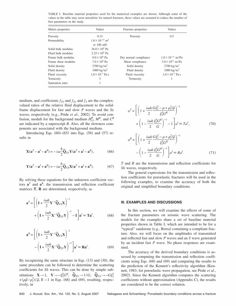
TABLE I. Baseline material properties used for thevalues in the table may seem unrealistic for natural frfree parameters in the study.

Matrix properties Values

Porosity 0.15Permeability 1.0�10−13 m2

or 100 mDSolid bulk modulus 36.0�109 PaFluid bulk modulus 2.25�109 PaFrame bulk modulus 9.0�109 PaFrame shear modulus 7.0�109 PaSolid density 2700 kg/m3

Fluid density 1000 kg/m3

Fluid viscosity 1.0�10−3 Pa sTortuosity 3Saturation ratio 1

tively, in

840 J. Acoust. Soc. Am., Vol. 122, No. 2, August 2007 Nakagawa

aT = �1 +i�h

2

G�12 − � + � f

2/�

�3SGB �−1

+ 1 −i�h

2

�3SGB

G�−1

− 1�aI � TaI, �70�

aR = �1 +i�h

2

G�12 − � + � f

2/�

�3SGB �−1

− 1 −i�h

2

�3SGB

G�−1�aI � RaI. �71�

T and R are the transmission and reflection coefficients forSh waves, respectively.

The general expressions for the transmission and reflec-tion coefficients for poroelastic fractures will be used in thefollowing examples, to examine the accuracy of both theoriginal and simplified boundary conditions.

III. EXAMPLES AND DISCUSSIONS

In this section, we will examine the effects of some ofthe fracture parameters on seismic wave scattering. Themodels for the examples share a set of baseline materialproperties shown in Table I, which are intended to be for a“typical” sandstone �e.g., Berea� containing a compliant frac-ture. Also, we will focus on the amplitudes of transmittedand reflected fast and slow P waves and an S wave generatedby an incident fast P wave. No phase responses are exam-ined.

The accuracy of the derived boundary conditions is as-sessed by computing the transmission and reflection coeffi-cients using Eqs. �68� and �69� and comparing the results tothe prediction of the Kennett’s reflectivity algorithm �Ken-nett, 1983; for poroelastic wave propagation, see Pride et al.,2002�. Since the Kennett algorithm computes the scatteringcoefficients without approximation �Appendix C�, the results

erical examples are shown. Although some of thees, these values are assumed to reduce the number of

Fracture properties Values

Porosity 0.5

ry normal compliance 1.0�10−11 m/PaShear compliance 3.0�1011 m/Pa

Solid density 2700 kg/m3

Fluid density 1000 kg/m3

Fluid viscosity 1.0�10−3 Pa sTortuosity 1

numactur

D

are considered to be the correct solution.

and Schoenberg: Poroelastic boundary conditions across a fracture

A. Impact of pressure diffusion within a fracture

In the first example, we examine the accuracy of theporoelastic fracture boundary conditions in Eq. �30� and theimpact of the fluid pressure dissipation factor � in Eq. �21�on wave scattering. For this example, in addition to the prop-erties shown in Table I, we assume both high fracture per-meability k0=10−10 m2 �100 D; 1000 times the backgroundpermeability� and low fracture permeability k0=10−16 m2

�0.1 mD; 0.001 times the background permeability�, with afracture thickness h=1 mm. The fracture is fully saturatedwith the same fluid as the background, and the bulk modulusof the solid �grains� is also the same as the background.

Both normal-incidence frequency responses for a fre-quency range of 10 Hz to 1 MHz—Figs. 5�a� and 5�b�—andangle-of-incidence responses at 1 kHz—Figs. 5�c� and5�d�—show very good agreement between the Kennett algo-

FIG. 5. Amplitudes of the displacement transmission and reflection coefficbackground� and high-permeability �1000� background� fractures with a thicoefficient, with subscript Pf=fast P wave, Ps=slow P wave, and S=S wavdotted curves were computed using the full fracture model in Eq. �30� with anfactor �, respectively. For the high-permeability fracture, the correction is nby Kennett method. However, for the low-permeability fracture, the modelresponse. k0=10−10 m2; �b� Normal incidence frequency response. k0=10−1

incidence response. k0=10−16 m2.

rithm �shown in discrete symbols� and the full fracture model

J. Acoust. Soc. Am., Vol. 122, No. 2, August 2007 Nakagawa and Sc

�shown in thick solid lines�. The errors seen above 100 kHzfor the normal incidence case result primarily from the mul-tiple scattering of waves within the fracture �layer�, which isnot accounted for by the fracture model. An approximatefrequency corresponding to the lowest-frequency resonance�reverberation� of the fast P wave within the fracture is in-dicated in the plots by an arrow.

When the effect of pressure diffusion within a fracture isignored by enforcing the fluid-pressure dissipation factor �

=1 in Eqs. �30�–�41�, the fracture model �shown by dottedlines in Fig. 5� significantly overestimates the reflected fast Pwave �Figs. 5�b� and 5�d�� and scattered slow P waves for alow-permeability fracture above a frequency near 10 Hz.This frequency is a transient �critical� frequency that sepa-rates the drained and undrained response of a fracture. �Moredetailed discussion will be given later in Sec. III C.� In con-

for incident fast P waves computed for both low-permeability �1/1000�s h=1 mm. The labels indicate T=transmission coefficient and R=reflectioniscrete symbols were computed by the Kennett method.� Solid curves and

thout the correction of the pressure diffusion by the fluid pressure dissipationible, and both models agree very well with the “correct solution” computedut the correction shows significant errors. �a� Normal incidence frequency�c� 1-kHz angle-of-incidence response. k0=10−10 m2; �d� 1-kHz angle-of-

ientscknese. �Dd wiegligwitho6 m2;

hoenberg: Poroelastic boundary conditions across a fracture 841

=1 cm; �c� h=10 cm.

trast, for a high-permeability fracture, ignoring the effect ofpressure diffusion does not result in noticeable errors �Figs.5�a� and 5�c��.

B. Fracture thickness and the accuracy of fracturemodels

We derived the simplified fracture model in Eq. �67� byassuming that the O�h� terms in the original boundary con-ditions can be ignored except for the characteristic param-eters of a fracture. For a finite fracture thickness, however,this assumption has to be scrutinized.

In the following example, we assume a set of character-istic fracture parameters �T=3�10−11 m/Pa, �ND

=1

�10−11 m/Pa, �=0.85, B=0.29, and �0=k0 /h=1�10−13 m,and examine the effect of fracture thickness on the wavescattering for three thickness values: h=1 mm, 1 cm, and10 cm. These characteristic parameters were chosen for thetypical physical parameters in Table I, assuming that the 10-cm-thick fracture was 100% saturated by the same fluid asthe background. �The bulk modulus of the fluid in the thinner

fractures has to be reduced to maintain the same � and Bvalues, which can be realized physically by introducing asmall amount of gas in the fluid.� Elastic properties of thematerial within the fracture are determined from these pa-rameters as a function of fracture thickness and used in thefull fracture model in Eqs. �30�–�41� as well as the layermodel.

In this example, we also examine the accuracy of thesimplified fracture model in Eq. �52� compared to the fullfracture model and the layer solution of Kennett’s reflectivityalgorithm. Reflection and transmission coefficient ampli-tudes for fast and slow P waves generated from normallyincident fast P waves are shown in Fig. 6. For thin fracturethickness h below 1 cm, both full and simplified fracturemodels agree very well with the layer model, with the upperlimit of applicable range of frequency reducing with increas-ing h. The error becomes large near and above the first reso-nance frequency of the fast P wave within the fracture, asindicated by a gray vertical line in the plots. The resonancefrequencies for this example are lower than the previous ex-ample, because the combination of material properties usedhere yields large undrained fracture compliance, which re-sults in slower fast P-wave velocity within the fracture. Fur-ther, for the h=10-cm case, the reflected fast P wave is in-accurately predicted by the simplified model, even wellbelow the resonant frequency. This is probably caused by theeffect of mass within the layer. This effect is neglected in thesimplified model, since the scattering of slow P waves,which is predominantly governed by the diffusion of fluidpressure within the pore space, is still accurately predicted.

Because the characteristic fracture parameters are notdependent on fracture thickness, the simplified model showsidentical responses in Figs. 6�a�–6�c� �shown by thin solidlines�. The slight differences in the transmitted slow P-waveresponse predicted by the model in Fig. 6�c� compared to

Figs. 6�a� and 6�b� result from the complex dependence of

842 J. Acoust. Soc. Am., Vol. 122, No. 2, August 2007 Nakagawa

FIG. 6. Normal-incidence reflection and transmission coefficient amplitudesfor fast and slow P waves for the same characteristic fracture parametersand three values of fracture thickness. For thin fracture thickness �below1 cm�, both full and simplified fracture models agree very well with thelayer model, with the upper limit of the applicable range of frequency re-ducing with increasing h. For the h=10 cm case, the reflected fast P wave isinaccurately predicted by the simplified model, possibly because of the ef-fect of mass within the layer, which is not considered. �a� h=1 mm; �b� h

and Schoenberg: Poroelastic boundary conditions across a fracture

dynamic permeability on h at high frequencies for a givenstatic membrane permeability �defined by Eq. �44�, with afrequency ��0�.

C. Effect of fracture permeability on seismic wavescattering

In the third example, we repeat our experiment of thefirst example to further examine the effect of fracture hy-draulic permeability �or membrane permeability�. The mate-rial properties and fracture thicknesses used here are thesame as in the first example �h=1 mm�, which results incharacteristic fracture parameters �T=3�10−11 m/Pa, �ND

=1�10−11 m/Pa, �=0.998, and B=0.98.The scattering amplitudes are computed using the sim-

plified fracture model in Eq. �52� for a wide range of mem-brane permeability values �Fig. 7�. To examine the behaviorof the waves more closely, each wave and scattering mode isshown separately. We also compute the high-and low-permeability limits of the scattering responses using Eq. �53�

FIG. 7. Scattering amplitude responses �scattering coefficients� for a range oshown with semi-log scales to clearly show changes at large amplitudes. Dfracture. Different membrane permeability values correspond to different typtransmission; �b� Fast P-wave reflection; �c� Slow P-wave transmission; �d�

and Eq. �54�, respectively, which are shown in thick dotted

J. Acoust. Soc. Am., Vol. 122, No. 2, August 2007 Nakagawa and Sc

lines bounding finite-permeability responses �except for thezero-permeability bound in the slow P-wave reflection inFig. 7�d�, for which the scattering response of a low-permeability fracture is more complicated and undershootsthe low-permeability limit�.

A distinct characteristic of the reflected fast P wave andboth transmitted and reflected slow P waves is that the slopechanges when each frequency response curve departs fromthat of the high-permeability limit �labeled as �0=��. Forexample, for �0=10−13 m �corresponding to the case previ-ously shown in Fig. 5�b��, this occurs near 10 Hz. For asaturated fracture with high, dry compliance, this transition�critical� frequency can be evaluated as follows:

From Eq. �51�,

� �1 − i

2��

�2� f�ND

2�0B. �72�

From the behavior of ���� shown in Fig. 3, the transitionfrequency �critical frequency� �d between the drained and

brane permeability of a fracture. Fast P-wave transmission coefficients arelines are both for a fracture with infinite permeability and an impermeablees that “saturate” at both low and high permeability values. �a� Fast P-waveP-wave reflection.

f memottede curv

Slow

undrained responses of a low-permeability fracture is evalu-

hoenberg: Poroelastic boundary conditions across a fracture 843

ated by a frequency corresponding to Re���=1, resulting in

�d =�0

� f

8B

�2�ND

, �73�

which is proportional to the membrane permeability of afracture and inversely proportional to the dry normal compli-ance of the fracture. When the parameter values used in thisexample are introduced with �0=10−13 m, the characteristicfrequency is fd=�d /2�=12.7 Hz, which is close to the10 Hz observed in both Fig. 5�b� and Figs. 7�b�–7�d�. Also,�d can be viewed as a critical frequency below which thereflection of fast P waves and the scattering of slow P wavesbecome insensitive to the changes in fracture permeability.Conversely, if the permeability of the fracture is low, for agiven frequency, membrane permeability higher than the fol-lowing critical permeability cannot be determined using seis-mic waves from the scattering of plane waves,

�0c =�� f�

2�ND

8. �74�

At 1 kHz, the critical membrane permeability is �0c=7.9�10−12 m.

IV. CONCLUSIONS

A fluid-filled, flat fracture is a special case of heteroge-neous poroelastic media, for which the effect of poroelasticmaterial properties on discrete scattering of seismic wavescan be examined analytically, owing to its simple geometry.We hypothesize that a compliant fracture can be viewed as aflat, thin, soft inclusion within a matrix. This simplificationresults in sets of boundary conditions relating a finite jump inthe stress and velocity across a fracture to the stress andvelocity at the boundaries �fracture surfaces�.

The key step in the derivation of the boundary condi-tions is the approximation of the pressure field within a frac-ture: although the thickness of a fracture can usually be con-sidered much smaller than the wavelength of an incomingwave �fast P wave and S wave�, the pressure diffusion length�or the wavelength of the generated slow wave� within thefracture can be comparable to the fracture thickness, result-ing in a rapid change in the pressure distribution. In turn, thiscomplex pressure distribution due to diffusion affects howthe wave is scattered, as a function of permeability and fluidproperties within the fracture.

For a thin fracture, however, the permeability parallel tothe fracture cannot be resolved from the wave scattering, asindicated by the results in Appendix A. In this case, thepermeability needs to be inferred indirectly from the dry andwet fracture compliances—parameters which depend on afracture’s internal structure �such as porosity, asperity, con-tact spacing�, which also affects the permeability. In contrast,fracture-normal permeability can affect wave scattering if thepermeability is below a threshold value and the wave fre-quency is above a critical frequency.

Typically, the scattering behavior of a fracture changesat a frequency where the fluid-solid interaction within the

fracture changes between drained �low frequency and high

844 J. Acoust. Soc. Am., Vol. 122, No. 2, August 2007 Nakagawa

permeability� and undrained �high frequency and low perme-ability� regimes. In general, for a normally incident fast Pwave, a fracture with higher fracture-normal permeability ex-hibits larger reflection of fast P waves and generates moreslow P waves. However, amplitudes of slow P waves gener-ated by a single fracture are generally small. For the effect tobe clearly measurable, high-frequency seismic waves and/ormultiple fractures may be necessary.

The scattering of waves by a fracture is controlled by aset of characteristic �phenomenological� parameters similarto the fracture compliance used in the linear slip interfacemodel �Schoenberg, 1980�. These parameters are shear com-pliance, drained normal compliance, Biot-Willis effectivestress coefficient, fracture Skempton coefficient, and mem-brane permeability. For a sufficiently small fracture thick-ness, fractures having identical parameter values result in thesame observed seismic response.

Finally, throughout the modeling presented in this paper,a fracture is assumed to be an isotropic and homogeneouslayer. �An extension of the model to anisotropic elasticmoduli and permeability is presented in Appendix A.� Thequestion remains, can an open fracture with partial surfacecontacts and a fault with complex internal geometry be mod-eled with such a simple model? For example, scattering ofwaves may be strongly affected by the local fluid motionaround contacting asperities and within the complex internalstructure of a well-developed fault originating from shearing�e.g., Sibson, 1977�. For such cases, more complex boundaryconditions, considering the effect of internal heterogeneity ofa fracture, are necessary.

ACKNOWLEDGMENTS

This research has been supported by the Office of Sci-ence, Office of Basic Energy Sciences, Division of ChemicalSciences of the U.S. Department of Energy under ContractNo. DE-AC76SF00098. The authors would like to thank Dr.Steven Pride at Lawrence Berkeley National Laboratory formany useful suggestions and discussions during the develop-ment of the models presented in this article.

APPENDIX A: DERIVATION OF SEISMIC BOUNDARYCONDITIONS FOR A TRANSVERSELY ISOTROPICPOROELASTIC FRACTURE

Constitutive relationships for a general anisotropic po-roelastic medium can be written using index notations as�Cheng, 1997�

�ij = CijklD uk,l + �ij�− pf� = Cijkl

U uk,l + M�ijwk,k, �A1�

− pf = M�wk,k + �ijui,j� , �A2�

where �ij is the symmetric Biot-Willis effective stress coef-ficient tensor and Cijkl

D and CijklU =Cijkl

D +M�ij�kl are the dry�drained� and undrained stiffness tensors for the solid frame,respectively. M is the fluid storage modulus. The momentumbalance equations are

2

�ij,j = − � ��ui + � fwi� , �A3�

and Schoenberg: Poroelastic boundary conditions across a fracture

− pf ,i = − �2�� fui + �ijwj� , �A4�

where �ij is defined via an anisotropic dynamic permeabilitytensor k��� through ���i� f /��k−1���.

For the following, we will focus on the transversely iso-tropic case with the axis of symmetry aligned in the 3 direc-tion �fracture-normal direction�. In the reduced matrix nota-tion, the above constitutive relationship becomes

��11

�22

�33

�23

�31

�12

= �C11

D C12D C13

D

C12D C11

D C13D

C13D C13

D C33D

G

G

G�

�u1,1

u2,2

u3,3

u2,3 + u3,2

u3,1 + u1,3

u1,2 + u2,1

+ �

�1

�1

�3

0

0

0

�− pf� , �A5�

h

J. Acoust. Soc. Am., Vol. 122, No. 2, August 2007 Nakagawa and Sc

− pf = M��1u1,1 + �1u2,2 + �3u3,3� + M�w1,1 + w2,2

+ w3,3� , �A6�

where G�= �C11D −C12

D � /2, and �i �i=1, 3� are the diagonalentries of the effective stress coefficient tensor �. The mo-mentum balance equation is the same as the general aniso-tropic case, except that the permeability tensor also becomesdiagonal: k���=diag�k1��� ,k1��� ,k3����, where each diag-onal component can be computed using the dynamic perme-ability model proposed by Johnson et al. �1987�. Followingthe same procedure as in the isotropic case, we obtain acounterpart to the governing equations Eqs. �5� and �6� withcoefficient matrices,

R � � 1/G

− G��12 + � −

� f2

�1 , �A7�

QXY � �1/G �1 0

�1 � � f

0 � � , �A8�

f 3

QYX � �� −

� f2

�1

− C11D −

C13D2

C33D ��1

2 �1C13

D

C33D �1�1 − �3

C13D

C33D −

� f

�1�

�1C13

D

C33D

1

C33D −

�3

C33D

�1�1 − �3C13

D

C33D −

� f

�1� −

�3

C33D

1

M+

�32

C33D −

1

�1

�12 . �A9�

Using Eqs. �A7�–�A9�, for a small fracture thickness h, for-mally identical simplified boundary conditions as in the iso-tropic case �Eqs. �46� and �52�� are obtained if the definitionsof the characteristic fracture parameters are modified as fol-lows:

�T �h

G, �A10�

�ND�

h

C33D , �A11�

� � �3, �A12�

���� �k3���

, �A13�

B ��3

C33D � 1

M+

�32

C33D � = �3

M

C33U . �A14�

Note that only the anisotropic material properties related tothe 3 direction �fracture-normal direction� appear in thesedefinitions, which indicates that the scattering of waves isnot affected by the quantities related to the fracture-paralleldirections �Specifically, permeability along the fracture�. Thefluid pressure dissipation factor � is the same as the isotro-pic case if the direction of the slow P-wave propagationwithin the fracture is approximately in the fracture-normaldirection. One important difference from the isotropic case,however, is that the normal and shear fracture compliancescan take arbitrary values independent from each other.

APPENDIX B: THE DYNAMIC PERMEABILITYOF OPEN AND VERY PERMEABLE FRACTURES

For a highly permeable fracture or an open fracture inwhich fluid flow parallel to the fracture can be affected bythe viscous friction along the fracture surfaces, the effective

permeability of the layer representing a fracture in the frac-

hoenberg: Poroelastic boundary conditions across a fracture 845

ture parallel direction must be reduced. As shown in Appen-dix A, for a transversely isotropic fracture �a layer modeling

the fracture is transversely isotropic�, QXY contains only the

fracture-normal permeability k3��� and QYX contains onlythe fracture-parallel permeability k1���. Therefore, for theisotropic fracture model discussed in the main body of thispaper, the permeability needs to be allowed to be anisotropic.

In discussing the high-permeability case, we are con-

cerned only with fracture-parallel permeability k1��� in QYX

because terms including k3��� in the boundary conditionsappear only as h /k3���, which become negligibly small forsmall hs. If fracture-parallel fluid flow within the fracture islaminar and the flow on the fracture surfaces can be ignoredbecause of the small permeability in the background, themaximum possible permeability for this fracture can beevaluated using Biot’s results for the dynamic permeabilityof plane parallel flows �Biot, 1956b�,

�k1���� � �kplane���� = � h2

4�21 −tanh �

��� , �B1�

� �h

2�� f�

i� f.

Therefore, the permeability for the flow in the fracture par-allel direction is bounded by taking the limit of Eq. �B1� forh→�

�k1���� � � h2

4�2� =� f

� f�. �B2�

Equation �B2� gives the maximum possible dynamic perme-ability of any fracture for a given fluid type. This limit canalso be obtained directly from the momentum balance equa-tion for an acoustic medium,

��− pf� = − �2� fU . �B3�

This equation can be rewritten as

U =i

�� f� �− pf� �

k���� f

� �− pf� . �B4�

Therefore, we identify the permeability as

k��� =i� f

�� f, �B5�

which is identical to Eq. �B2�. The same expression can alsobe obtained by bringing the static permeability k0 to infinityin the expression for in dynamic permeability given byJohnson et al. �1987�,

k��� = k0��1 − i4

nJ

�

�J− i

�

�J� , �B6�

where nJ is a finite parameter determined by the pore geom-etry �a value of 8 is recommended for common sandstones�,and �J is the viscous-boundary characteristic frequencygiven by �J�� f /� fFk0=� f� /� f��k0, where F is the electri-cal formation factor and �� is the high-frequency limit pore-space tortuosity, both of which approach unity for an open

fracture.

846 J. Acoust. Soc. Am., Vol. 122, No. 2, August 2007 Nakagawa

Using Eq. �B2� and the definition in Eq. �4�, we obtain

��� � ���k0 → � �� = � f . �B7�

This indicates that the magnitude of terms h / � in QYX isbounded by a negligibly small value h /� f for small h’s.Therefore, permeability in the fracture parallel direction doesnot appear in the seismic boundary conditions for any staticpermeability values of the medium and does not affect thescattering of seismic waves. Conversely, permeability of afracture in the fracture-parallel direction cannot be deter-mined from measured seismic responses if the fracture thick-ness is much smaller than the wavelength of propagatingseismic waves.

APPENDIX C: KENNETT’S REFLECTIVITYALGORITHM APPLIED TO A SINGLE POROELASTICLAYER

Pride et al. �2002� applied Kennett’s reflectivity algo-rithm �Kennett, 1983� to piecewise-homogeneous layeredporoelastic media. Exact expressions for the transmissionand reflection coefficients of a single poroelastic layer repre-senting a fracture can be obtained as a special case of theapplication.

Kennett method is based upon the following recursiverelationships between the transmission and reflection coeffi-cients for a group of n parallel interfaces and coefficients, forthe remaining n−1 interfaces after the first interface in theseries is removed:

T�n� = T�n−1�En�I − Rn−EnR�n−1�En�−1Tn

+, �C1�

R�n� = Rn+ + Tn

−EnR�n−1�En�I − Rn−EnR�n−1�En�−1Tn

+, �C2�

where the transmission and reflection coefficient matrices forthe removed interface are given as Tn and Rn, respectively,with a sign in the superscript indicating the incident wavedirection. T�n�, T�n−1�, R�n�, and R�n−1� are for the n and n−1 interfaces, as indicated in the parentheses, and for inci-dent waves propagating in the positive direction. En is thediagonal-phase advance matrix between the interfaces.

For the case of a single layer �two interfaces�, no recur-sion is necessary to compute the transmission and reflectioncoefficients T and R for the whole system. By setting T�0�

=T0+, R�0�=R0

+, T=T�1�, and R=R�1�,

T = T0+E�I − R1

−ER0+E�−1T1

+, �C3�

R = R1+ + T1

−ER0+E�I − R1

−ER0+E�−1T1

+. �C4�

For in-plane wave propagation �fast and slow P waves and Swaves with particle motions parallel to the plane of wavepropagation�, these matrices correspond to the transmissionand reflection coefficient matrices in Eqs. �68� and �69�. The

phase advance matrix is E�diag�ei��zPfh ei��z

Psh ei��zSh�. The

transmission and reflection coefficient matrices for the indi-vidual interfaces are a function of material properties forboth the background and the fracture layer, which results invery complex expressions for Eqs. �C3� and �C4� �albeit theyare in closed form�. These equations are evaluated numeri-

cally to obtain “correct solutions” in the example presented

and Schoenberg: Poroelastic boundary conditions across a fracture

in this paper. The interface scattering matrices can be com-puted, for example, using the equations presented by Pride etal. �2002�.

Adams, J. T., and Dart, C. �1998�. “The appearance of potential sealingfaults on borehole images,” in Faulting, Fault Sealing and Fluid Flow inHydrocarbon Reservoirs, edited by G. Jones, Q. J. Fisher, and R. J. Knipe,Geol. Soc. Spec. Publ. 147, 71–86.

Aydin, A. �1978�. “Small faults formed as deformation bands in sandstone,”Pure Appl. Geophys. 116, 913–930.

Bakulin, A., and Molotkov, L. �1997�. “Poroelastic medium with fracturesas limiting case of stratified poroelastic medium with thin and soft Biotlayers,” 67th Annual International Meeting, SEG, Expanded Abstracts,1001–1004.

Bakulin, A., Grechka, V., and Tsvankin, I. �2000�. “Estimation of fractureparameters from reflection seismic data. I. HTI model due to a singlefracture set,” Geophysics 65, 1788–1802.

Berryman, J. G., and Wang, H. F. �1995�. “The elastic coefficients ofdouble-porosity models for fluid transport in jointed rock,” J. Geophys.Res. 100, 24611–24627.

Berryman, J. G., and Wang, H. F. �2000�. “Elastic wave propagation andattenuation in a double-porosity dual-permeability medium,” Int. J. RockMech. Min. Sci. 37, 63–78.

Biot, M. A. �1956a�. “Theory of elastic waves in a fluid-saturated poroussolid. I. Low frequency range,” J. Acoust. Soc. Am. 28, 168–178.

Biot, M. A. �1956b�. “Theory of elastic waves in a fluid-saturated poroussolid. II. High frequency range,” J. Acoust. Soc. Am. 28, 179–191.

Brajanovski, M., Gurevich, B., and Schoenberg, M. �2005�. “A model forP-wave attenuation and dispersion in a porous medium permeated byaligned fractures,” Geophys. J. Int. 163, 372–384.

Cheng, A. H.-D. �1997�. “Material coefficients of anisotropic poroelastic-ity,” Int. J. Rock Mech. Min. Sci. 34�2�, 199–205.

Coates, R. T., and Schoenberg, M. �1995�. “Finite-difference modeling offaults and fractures,” Geophysics 60�5�, 1514–1526.

Dutta, N. C., and Odé, H. �1979a�. “Attenuation and dispersion of compres-sional waves in fluid-filled porous rocks with partial gas saturation �WhiteModel�–I. Biot theory,” Geophysics 44, 1777–1788.

Dutta, N. C., and Odé, H. �1979b�. “Attenuation and dispersion of compres-sional waves in fluid-filled porous rocks with partial gas saturation �WhiteModel�–II. Results,” Geophysics 44, 1806–1812.

Gelinsky, S., and Shapiro, S. A. �1997�. “Dynamic-equivalent medium ap-proach for thinly layered saturated sediments,” Geophys. J. Int. 128, F1–F4.

Gurevich, B., Marschall, R., and Schapiro, S. A. �1994�. “Effect of fluidflow on seismic reflections from a thin layer in a porous medium,” J.Seism. Explor. 3, 125–140.

Gurevich, B., Zyrianov, V. B., and Lopatnikov, S. L. �1997�. “Seismic at-tenuation in finely layered porous rocks: Effects of fluid flow and scatter-ing,” Geophysics 62�1�, 319–324.

Gurevich, B., and Schoenberg, M. A. �1999�. “Interface conditions for Bi-ot’s equations of poroelasticity,” J. Acoust. Soc. Am. 105�5�, 2585–2589.

Haskell, N. A. �1953�. “The dispersion of surface waves in multilayered

J. Acoust. Soc. Am., Vol. 122, No. 2, August 2007 Nakagawa and Sc

media,” Bull. Seismol. Soc. Am. 43, 17–34.Hsu, C.-J., and Schoenberg, M. A. �1993�. “Acoustic waves through a simu-

lated fractured medium,” Geophysics 58�7�, 964–977.Johnson, D. L. �2001�. “Theory of frequency dependent acoustics in patchy-

saturated porous media,” J. Acoust. Soc. Am. 110�2�, 682–694.Johnson, D. L., Koplik, J., and Dashen, R. �1987�. “Theory of dynamic

permeability and tortuosity in fluid-saturated porous media,” J. FluidMech. 176, 379–402.

Kennett, B. L. N. �1983�. Seismic Wave Propagation in Stratified Media�Cambridge University Press, Cambridge�.

Nakagawa, S., Nihei, K. T., and Myer, L. R. �2002�. “Elastic wave propa-gation along a set of parallel fractures,” Geophys. Res. Lett. 29, 31-1–31-4.

Nihei, K. T., Weidong, Y., Myer, L. R., Cook, N. G. W., and Schoenberg, M.A. �1999�. “Fracture channel waves,” J. Geophys. Res. 104�B3�, 4769–4781.

Norris, A. N. �1993�. “Low-frequency dispersion and attenuation in partiallysaturated rocks,” J. Acoust. Soc. Am. 94, 359–370.

Pride, S. R., Tromeur, E., and Berryman, J. G. �2002�. “Biot slow-waveeffects in stratified rock,” Geophysics 67�1�, 271–281.

Pride, S. R. �2003�. “Relationships between seismic and hydrological prop-erties,” in Hydrogeophysics, edited by Y. Rubin and S. Hubbard �KluwerAcademic, New York�, pp. 1–31.

Pride, S. R., and Berryman, J. G. �2003a�. “Linear dynamics of double-porosity and dual-permeability materials, I. Governing equations andacoustic attenuation,” Phys. Rev. E 68, 036603.

Pride, S. R., and Berryman, J. G. �2003b�. “Linear dynamics of double-porosity and dual-permeability materials. II. Fluid transport equation,”Phys. Rev. E 68, 036604.

Pyrak-Nolte, L. J., and Cook, N. G. W. �1987�. “Elastic interface wavesalong a fracture,” Geophys. Res. Lett. 14�11�, 1107–1110.

Pyrak-Nolte, L. J., and Morris, J. P. �2000�. “Single fractures under normalstress: The relation between fracture specific stiffness and fluid flow,” Int.J. Rock Mech. Min. Sci. 37, 245–262.

Pyrak-Nolte, L., Cook, N. G. W., and Myer, L. R. �1990�. “Transmission ofseismic waves across single natural fractures,” J. Geophys. Res. 95, 8516–8538.

Rokhlin, S. I., and Wang, Y. J. �1991�. “Analysis of boundary conditions forelastic wave interaction with an interface between two solids,” J. Acoust.Soc. Am. 89�2�, 503–515.

Schoenberg, M. A. �1980�. “Elastic wave behavior across linear slip inter-faces,” J. Acoust. Soc. Am. 68, 1516–1521.

Schoenberg, M. A., and Protazio, J. �1992�. “Zoeppritz rationalized andgeneralized to anisotropy,” J. Seism. Explor. 1�2�, 125–144.

Schoenberg, M. A., and Sayers, C. M. �1995�. “Seismic anisotropy of frac-tured rock,” Geophysics 60, 204–211.

Shapiro, S. A., and Müller, T. M. �1999�. “Seismic signatures of permeabil-ity in heterogeneous porous media,” Geophysics 64�1�, 99–103.

Sibson, R. H. �1977�. “Fault rock and fault mechanisms,” J. Geol. Soc.�London� 133, 191–213.

White, J. E., Mikhahaylova, N. G., and Lyakhovistsky, F. M. �1975�. “Low-frequency seismic waves in fluid-saturated layered rocks,” Izv., Acad. Sci.,

USSR, Phys. Solid Earth 11, 654–659.

hoenberg: Poroelastic boundary conditions across a fracture 847