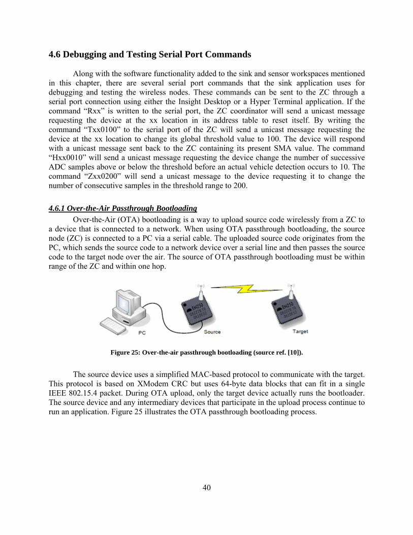
Portable Cellular Wireless Mesh Sensor Network for … Cellular Wireless Mesh Sensor Network for...

Portable Cellular Wireless Mesh Sensor Network for Vehicle Tracking in an Intersection

Final Report

Prepared by:

Taek Mu Kwon Ryan Weidemann

Transportation Data Research Laboratory Northland Advanced Transportation Systems Research Laboratories

Department of Electrical and Computer Engineering University of Minnesota, Duluth

CTS 08-29

Technical Report Documentation Page 1. Report No. 2. 3. Recipients Accession No. CTS 08-29 4. Title and Subtitle 5. Report Date

December 2008 6. Portable Cellular Wireless Mesh Sensor Network for Vehicle

Tracking in an Intersection 7. Author(s) 8. Performing Organization Report No. Taek Mu Kwon and Ryan Weidemann 9. Performing Organization Name and Address 10. Project/Task/Work Unit No.

CTS Project # 2007039 11. Contract (C) or Grant (G) No.

Department of Electrical and Computer Engineering University of Minnesota- Duluth 1023 University Drive Duluth, Minnesota 55812

12. Sponsoring Organization Name and Address 13. Type of Report and Period Covered Final Report 14. Sponsoring Agency Code

Intelligent Transportation Systems Institute Center for Transportation Studies University of Minnesota 511 Washington Avenue SE, Suite 200 Minneapolis, Minnesota 55455

15. Supplementary Notes http://www.cts.umn.edu/Publications/ResearchReports/ 16. Abstract (Limit: 200 words) This report describes the result of a research project that developed an automatic, portable vehicle tracking system that can count the vehicle travel trajectories in an intersection. Using a cellular wireless mesh sensor network (WMSN), wireless sensor nodes are placed in the middle of traffic lanes in the intersection to collect the data. Each node consists of an anisotropic magnetoresistance (AMR) circuit for detecting vehicles, a PAN4570 Radio Communications Module (RCM), and a lithium-ion rechargeable battery. When a vehicle travels over a wireless node, a detection occurs and a timestamp is recorded by the node and sent to the WMSN coordinator. The coordinator is responsible for logging the vehicle detections recorded by every node in the WMSN. From this logged data, a vehicle tracking algorithm that has been developed tracks the trajectories of the vehicles through the intersection and also records a total vehicle count of the intersection. The system performance was evaluated through both intersection simulations and real data collection. The details on the system component design, implementation, experimental results, and analysis are described.

17. Document Analysis/Descriptors 18. Availability Statement Wireless sensor network, ZigBee mesh, vehicle tracking. No restrictions. Document available from:

National Technical Information Services, Springfield, Virginia 22161

19. Security Class (this report) 20. Security Class (this page) 21. No. of Pages 22. Price Unclassified Unclassified 85

Portable Cellular Wireless Mesh Sensor Network for Vehicle Tracking in an Intersection

Final Report

Prepared By

Taek Mu Kwon Ryan Weidemann

Transportation Data Research Laboratory Northland Advanced Transportation Systems Research Laboratories

Department of Electrical and Computer Engineering University of Minnesota, Duluth

December 2008

Published By

Intelligent Transportation Systems Institute Center for Transportation Studies

200 Transportation and Safety Building 511 Washington Avenue S.E.

Minneapolis, Minnesota 55455

The contents of this report reflect the views of the authors, who are responsible for the facts and the accuracy of the information presented herein. This document is disseminated under the sponsorship of the Department of Transportation University Transportation Centers Program, in the interest of information exchange. The U.S. Government assumes no liability for the contents or use thereof. This report does not necessarily reflect the official views or policy of the Northland Advanced Transportation Systems Research Laboratories, the Intelligent Transportation Systems Institute or the University of Minnesota. The authors, the Northland Advanced Transportation Systems Research Laboratories, the Intelligent Transportation Systems Institute, the University of Minnesota and the U.S. Government do not endorse products or manufacturers. Trade or manufacturers' names appear herein solely because they are considered essential to this report.

ACKNOWLEDGEMENTS

The authors wish to acknowledge those who made this research possible. The study was

funded by the Intelligent Transportation Systems (ITS) Institute, a program of the University of Minnesota’s Center for Transportation Studies (CTS). Financial support was provided by the United States Department of Transportation Research and Innovative Technologies Administration (RITA).

The project was also supported by the Northland Advanced Transportation Systems Research Laboratories (NATSRL), a cooperative research program of the Minnesota Department of Transportation, ITS Institute, and the University of Minnesota Duluth College of Science and Engineering.

TABLE OF CONTENTS

Chapter 1: Introduction................................................................................................................. 1

1.1 Motivation and Objective ................................................................................................................ 1 1.2 Related Work .................................................................................................................................... 1

Chapter 2: Wireless ZigBee Technology....................................................................................... 3

2.1 ZigBee Stack Architecture ............................................................................................................... 3 2.1.1 Physical Layer.............................................................................................................................................4 2.1.2 Medium Access Control Layer ...................................................................................................................5 2.1.3 Network Layer ............................................................................................................................................5 2.1.4 Application Layer........................................................................................................................................5 2.1.5 Application Support Sub-Layer ..................................................................................................................5

2.2 Mesh Network Topology .................................................................................................................. 5 2.2.1 Definition of a Mesh Network ....................................................................................................................6 2.2.2 Mesh Network Nodes..................................................................................................................................6

2.3 ZigBee Mesh Network Routing ....................................................................................................... 7 2.4 Other Wireless Technologies ........................................................................................................... 8

Chapter 3: Node Hardware Design............................................................................................. 11

3.1 Anisotropic Magnetoresistance Sensor......................................................................................... 11 3.2 Panasonic PAN4570 Module.......................................................................................................... 14 3.3 Low Dropout Voltage Regulator ................................................................................................... 15 3.4 Lithium-Ion Rechargeable Battery ............................................................................................... 15 3.5 PADS Software ............................................................................................................................... 16

3.5.1 PADS Logic ..............................................................................................................................................17 3.5.2 PADS Layout ............................................................................................................................................17

3.6 Wireless Node Prototype................................................................................................................ 18 3.6.1 CircuitCAM ..............................................................................................................................................19 3.6.2 LPKF ProtoMat S62 Plotter ......................................................................................................................19 3.6.3 LPKF ProConduct and LPKF ProMask ....................................................................................................20 3.6.4 Final Wireless Node Prototype .................................................................................................................20 3.6.5 Wireless Node Bill of Materials................................................................................................................21

3.7 Wireless Router Prototype............................................................................................................. 22 3.8 Battery Charger Circuit................................................................................................................. 22

3.8.1 Final Battery Charger Circuit ....................................................................................................................26 3.8.2 Battery Charger Circuit Bill of Materials..................................................................................................27

3.9 Wireless Node Housing .................................................................................................................. 28 Chapter 4: Node Software Design............................................................................................... 31

4.1 Sink Advertise ................................................................................................................................. 32 4.2 Clock Synchronization ................................................................................................................... 33

4.2.1 Mock et al. Clock Synchronization Protocol.............................................................................................34 4.2.2 Mock et al. Examples................................................................................................................................35

4.3 Simple Moving Average ................................................................................................................. 36 4.4 Sampling the Analog-to-Digital Converter .................................................................................. 37 4.5 Logging of Vehicle Detections........................................................................................................ 38 4.6 Debugging and Testing Serial Port Commands........................................................................... 40

4.6.1 Over-the-Air Passthrough Bootloading.....................................................................................................40 Chapter 5: Intersection Simulator............................................................................................... 41

5.1 Cellular Division of an Intersection .............................................................................................. 41 5.2 Intersection Simulator Design ....................................................................................................... 42

5.2.1 Shifted Negative Exponential Distribution Function ................................................................................44 Chapter 6: Vehicle Tracking Algorithm ..................................................................................... 45

6.1 Elements of a Multiple Target Tracking System ......................................................................... 45 6.2 Modified Multiple Target Tracking System................................................................................. 46

6.2.1 Logged Vehicle Detections .......................................................................................................................47 6.2.2 Gating and Track Initiation .......................................................................................................................47 6.2.3 Track Association......................................................................................................................................48

6.3 Vehicle Tracking Algorithm Limitations ..................................................................................... 50 Chapter 7: Experimental Results ................................................................................................ 53

7.1 Intersection Simulator Testing ...................................................................................................... 53 7.2 Testing at the Real T-Intersection................................................................................................. 57

Chapter 8: Conclusions And Recommendations ........................................................................ 65

8.1 Conclusions ..................................................................................................................................... 65 8.2 Future Recommendations.............................................................................................................. 65

References .................................................................................................................................... 67

LIST OF TABLES

Table 1: Summary of PHY Layer Frequency Bands and Data Rates (source ref. [13])................. 4 Table 2: ZigBee Compared to Other Wireless Technologies (source ref. [16]) ............................. 9 Table 3: AMR Circuit Bill of Materials........................................................................................ 13 Table 4: Description of Used PAN4570 Pins ............................................................................... 14 Table 5: Wireless Node Bill of Materials ..................................................................................... 21 Table 6: Temperature Characteristics of the NTC Thermistor (source ref. [21]) ......................... 25 Table 7: LED Status (source ref. [21]).......................................................................................... 26 Table 8: Battery Charger Circuit Bill of Materials ....................................................................... 27 Table 9: ZC Address Table ........................................................................................................... 33 Table 10: Trajectory Entrance and Exit Nodes............................................................................. 43 Table 11: Vehicle Tracking Algorithm Incorrect Associations – Correct Trajectories................ 50 Table 12: Vehicle Tracking Algorithm Incorrect Associations – Incorrect Trajectories ............. 51 Table 13: Summary of Test-Site Intersection Roadway ADDT and Peak-Hour Values.............. 54 Table 14: Simulated Test-Site Intersection VPH Trajectory Counts............................................ 54 Table 15: Vehicle Tracking Algorithm Testing Using Simulated Intersection Data.................... 55 Table 16: Increased VPH Values.................................................................................................. 55 Table 17: Vehicle Tracking Algorithm Testing Using Increased VPH Values............................ 56 Table 18: Vehicle Tracking Results Using Original Test-Site Intersection Data......................... 60 Table 19: Vehicle Tracking Results Using Modified Test-Site Intersection Data ....................... 62 Table 20: Vehicle Tracking Results Using Modified Data and Incomplete Track Probability.... 63

LIST OF FIGURES

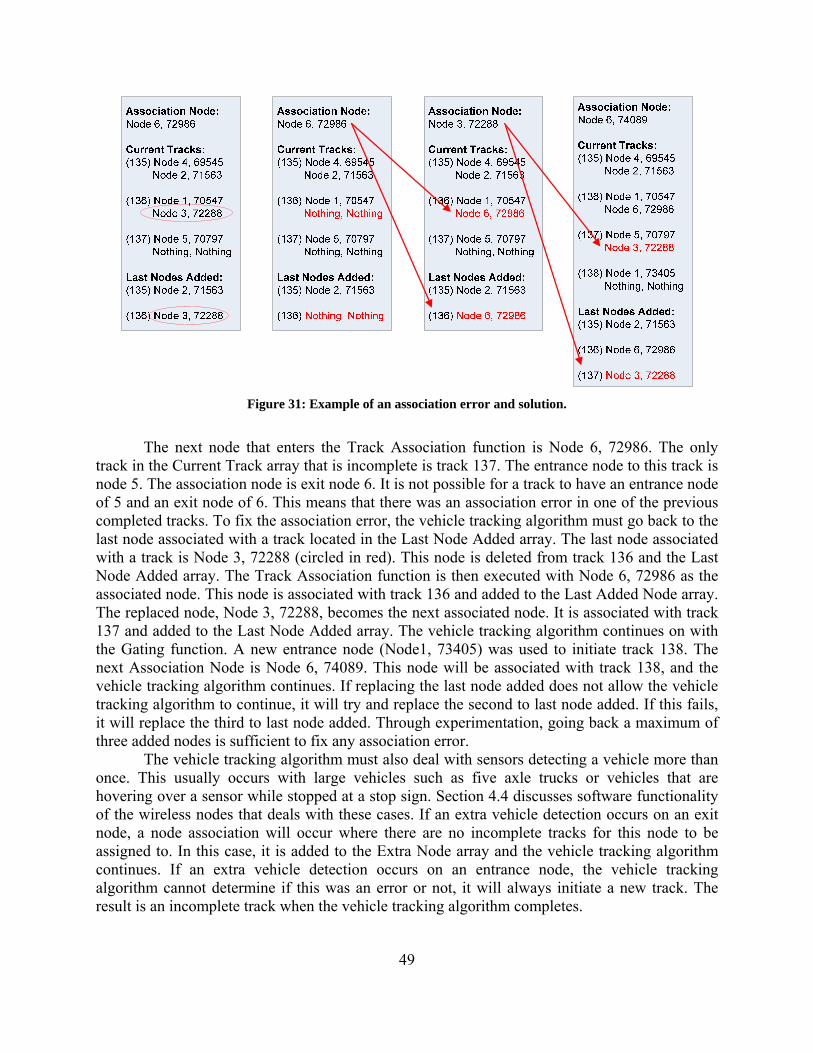
Figure 1: ZigBee stack architecture (source ref [12]). .................................................................... 4 Figure 2: A ZigBee WMSN (source ref. [14])................................................................................ 6 Figure 3: AMR element (left) 4-element Wheatstone bridge (right) (source ref [17])................. 12 Figure 4: Uniform magnetic field (left) magnetic field disturbance (right).................................. 12 Figure 5: PAN4570 module (source ref [19])............................................................................... 14 Figure 6: LDO voltage regulator circuit (source ref. [20]). .......................................................... 15 Figure 7: Wireless node PADS logic schematic. .......................................................................... 17 Figure 8: Wireless node PADS layout before routing. ................................................................. 18 Figure 9: Wireless node PADS layout after routing. .................................................................... 18 Figure 10: Wireless node CircuitCAM file................................................................................... 19 Figure 11: Wireless node prototype.............................................................................................. 21 Figure 12: Wireless router prototype ............................................................................................ 22 Figure 13: Li-ion battery charger circuit (source ref. [21]). ......................................................... 23 Figure 14: Battery charger circuit and li-ion rechargeable battery. .............................................. 27 Figure 15: Top, bottom, front, and side views of the wireless node housing. .............................. 29 Figure 16: Wireless node housing................................................................................................. 30 Figure 17: Wireless node inside a sensor housing. ....................................................................... 30 Figure 18: Main event loop (source ref. [10])............................................................................... 31 Figure 19: Mock et al. timing diagram (source ref. [24]). ............................................................ 34 Figure 20: Mock et al. clock synchronization protocol, example 1.............................................. 35 Figure 21: Mock et al. clock synchronization protocol, example 2.............................................. 36 Figure 22: Simple moving average example. ............................................................................... 37 Figure 23: Real-time data collector GUI. ..................................................................................... 39 Figure 24: Vehicle detection data collected on 10/4/08................................................................ 39 Figure 25: Over-the-air passthrough bootloading (source ref. [10])............................................. 40 Figure 26: Current (left) and original (right) intersection cellular configuration. ........................ 42 Figure 27: Intersection simulator GUI.......................................................................................... 43 Figure 28: MTT block diagram (source ref. [27]). ....................................................................... 45 Figure 29: Modified MTT block diagram for the vehicle tracking algorithm.............................. 46 Figure 30: Vehicle tracking GUI. ................................................................................................. 48 Figure 31: Example of an association error and solution. ............................................................ 49 Figure 32: Example 1 of a correct association (left) and an incorrect association (right). ........... 51 Figure 33: Example 2 of a correct association (left) and an incorrect association (right). ........... 52 Figure 34: Test-site intersection of Wallace Avenue and East 4th Street (source ref. [30]). ........ 53 Figure 35: Test-site intersection WMSN layout. ......................................................................... 57 Figure 36: Deploying a wireless node in the test-site intersection. .............................................. 58 Figure 37: Two deployed wireless nodes in the test-site intersection. ......................................... 59 Figure 38: NW trajectory cutting the corner................................................................................. 61

EXECUTIVE SUMMARY

The objective of this research project was to develop an automatic, portable vehicle tracking system that can count the vehicle travel trajectories in an intersection. Using a cellular wireless mesh sensor network (WMSN), wireless sensor nodes can be placed in the middle of traffic lanes in the intersection to collect the data. Each node consists of an anisotropic magnetoresistance (AMR) circuit for detecting vehicles, a PAN4570 Radio Communications Module (RCM), and a lithium-ion rechargeable battery. When a vehicle travels over a wireless node, a detection occurs and a timestamp is recorded by the node and sent to the WMSN coordinator. The coordinator is responsible for logging the vehicle detections recorded by every node in the WMSN. From this logged data, a vehicle tracking algorithm that has been developed can track the trajectories of the vehicles through the intersection and also record a total vehicle count of the intersection. Each node was designed and built using Mentor Graphics PADS software, CircuitCAM, and a LPKF ProtoMat S62 plotter. To protect the wireless node hardware, housings were built out of fiberglass. The shape of the housing resembles a raised pavement marker. This shape allows the wireless node to be protected if a vehicle happens to run over the sensor and also has a small profile so the sensor is not easily detected by drivers. A wireless sensor can be deployed in a matter of seconds using an adhesive spray to attach it to the pavement. It also can be collected very quickly by prying the wireless node from the pavement using only a screwdriver. Before any actual testing of the WMSN in an intersection can occur, the vehicle tracking algorithms must be developed and tested. A software simulation of an intersection has been created using Visual Basic programming language in Microsoft Visual Studio.NET 2003 environment. This intersection simulation allows a real intersection to be recreated and vehicle movements through the intersection to be simulated. The movements of vehicles through the intersection will produce logged data that is similar to the logged data of the actual WMSN. This logged data can then be used by the vehicle tracking algorithm to verify that the algorithm is tracking vehicles correctly before any actual data is collected. Along with verifying that the vehicle tracking algorithm works, the intersection simulator helps determine the minimum number of nodes that need to be deployed in an intersection, as well as the position of each node. The WMSN was deployed in an actual intersection. The intersection that was used for testing is a 2-lane T-intersection in Duluth, MN. The two roadways that form this test-site intersection are Wallace Avenue and East 4th Street. This T-intersection configuration required one coordinator, six wireless nodes located in the lanes of the intersection, and one wireless router. The wireless router’s purpose was to extend the range of the WMSN in order for wireless nodes located farthest from the coordinator to be able to communicate with the coordinator. Intersection data was collected for two time durations: 15 and 30 minutes. During data collection, a video camera was used to record traffic movements for ground truth verification, i.e., the results of the vehicle tracking algorithm are compared to the actual vehicle movements. Using the initial data, the vehicle tracking algorithm tracked vehicle trajectories with an error of 12.7% for a 15 minute time duration and an error of 10.1% for the time duration of 30 minutes. After reviewing the video footage of the data collection process, it was noticed that the layout of the WMSN could be changed to improve vehicle detection by repositioning two wireless nodes farther away from the intersection. Also, it was observed that 90% of traffic coming from the

north turned west instead of east. After the logged data was modified to account for this change in layout, and the vehicle tracking algorithm was modified, the results improved.

Based on the experimental results and the research presented, we conclude that the proposed WMSN system is a practical tool for accurately tracking vehicles in an intersection and can significantly save time and resources for intersection-justification data collection. With fine tuning of sensor detection ranges and positions, the research team is confident to predict that the present tracking accuracy of 90% can be improved to near 100%.

1

CHAPTER 1: INTRODUCTION

1.1 Motivation and Objective

More than 41% of all vehicle crashes in the US occur at intersections [1]. Of this 41% of crashes at intersection, 27% are at intersections with no control, stop sign or traffic signal, and 39% are at intersection with stop signs [1]. If an intersection has a history of vehicle crashes or increased traffic, it is up to a traffic engineer to determine if an upgrade to the intersection control is needed. The Minnesota Department of Transportation (Mn/DOT) has created the Intersection Control Evaluation (ICE) report, which replaced the Signal Justification Report in March, 2007, to assist traffic engineers in determining a viable alternative for intersection control.

In the Scoping Phase of the ICE report, data collection is an essential step. This data includes hourly intersection approach counts, turning movement counts for 3 hours for the AM and PM peak periods, among others [2]. Presently, engineers use handheld data collectors to collect this data. Using this approach, accuracy is difficult to achieve. Engineers must continuously monitor an intersection for a three-hour period constantly monitoring vehicles traveling through the intersection. For every vehicle that passes through the intersection, the engineer must be sure to press the corresponding button on the hand-held data collector according to the trajectory path observed. This demands a high degree of focus for an extended period of time. Furthermore, engineers monitoring intersections are on-site, which exposes them to weather and the chance of being struck by a vehicle. These factors lead to a loss of focus and in turn, a high degree of human error.

The nature of human error related to vehicle tracking was examined through simple counting tests. The authors of this research and Scott Klar (a research assistant) attempted to record vehicle trajectories through the intersection of Mesaba Avenue and Highway 53 in Duluth, MN. This is a four-way, eight-lane, traffic light controlled intersection with separate turning lanes. Shortly after the monitoring began, it was determined that an entire intersection could not be monitored by a single person. Human eye was not able to track simultaneous movements of many vehicles. We then focused our attention to monitoring only the north bound lane of Highway 53 for a period equal to length of a green light. Our objective was to count vehicles traveling north bound on Highway 53 and turning right to travel east bound on Mesaba Avenue. After three green light periods, our trajectory counts were compared. In two out of the three periods our counts did not match. Finally, we moved to West Arrowhead road, a simple two-lane street in Duluth. For ten minutes we monitored both east and west bound traffic. After the ten minute period ended, our east bound counts were 123, 120, and 120. Our west bound counts were 102, 105, and 101. These three simple vehicle trajectory counting experiments gave us first-hand experience in the difficulties of recording vehicle trajectories in the present method of vehicle tracking. This reaffirms the motivation behind this project.

1.2 Related Work

With U.S. DOT’s emphasis on intelligent transportation systems (ITS) in recent years, a wide range of traffic monitoring technologies for ITS have been researched and developed.

2

These technologies include video cameras [3, 4], microwave radars [5], passive infrared detectors [6], passive acoustic array sensors [7], and inductive loop detectors.

The most published research work on traffic tracking technology consists of a video camera(s) and digital image processing. There are many limitations associated with vehicle tracking using video cameras. First, video images are a two-dimensional representation of a three-dimensional space, resulting in a loss of depth information. Second, accurately identifying roads and vehicles from these two-dimensional images is very difficult. Occlusion is the main factor here. Third, the actual distance between objects is difficult to measure even if the objects are accurately detected. Fourth, visibility problems caused by weather such as snow, fog, and darkness limit the effectiveness of video cameras.

Besides video cameras and image processing, the developmental focus of the technologies listed above has been limited to point measurements on a roadway. Point measurement data provides only a small piece of traffic information. Traffic data collected using point measurements include volume, occupancy, and speed. Spatial traffic measurements, movements in two dimensional spaces in time, have long been the goal of traffic engineers. Previously, engineers have been using point measurements and estimation techniques to derive spatial measurements. However, these estimates proved to be only accurate on free flow traffic conditions, performing poorly when traffic congestion exists [8]. Spatial traffic measurements, such as detailed vehicle tracking in an intersection, are not feasible using conventional point measurement technologies.

Until recently, sensing technologies for spatial traffic measurements were unavailable, except video processing. Recent advances in wireless System-on-Chip (SoC) and magnetometer sensing technologies have enabled the opportunity to build small, cost-effective wireless sensors that can be deployed together in a wireless mesh sensor network (WMSN) to obtain spatial traffic measurements. The WMSN can be portable, temporary, and operate in a variety of environments and weather conditions.

Besides the present research being done on vehicle tracking systems, there is one commercially available product. Sensys Networks Inc. has developed a system that provides permanent count stations on highways and arterials, ramp management, stop bar detection, and systems counts including vehicle trajectories [9]. Components of this system include access points, repeaters, and wireless sensors. Similar to the proposed vehicle tracking system in this report, ZigBee wireless technology and magnetoresistive sensors are used. The main difference between the proposed system and Sensys is that Sensys uses Time Division Multiple Access (TDMA) instead of a wireless mesh network. In TDMA, each sensor is polled by an access point, requesting data from a sensor. If a sensor’s time slot is passed by, it must wait (latency) a minimum of 125 ms before it is polled again. This minimum latency will increase with the size of the network. More sensors in the network result in more time slots the access point must poll. Also, each node in the network is not capable of routing or forwarding data and an access point can only read data from a sensor that is one hop away. The result is a very limited coverage area. Furthermore, only 96 sensors are allowed to be connected to a single access point.

On the other hand, the proposed WMSN is a fully functioning mesh network that can route or forward packets of data using the optimal path without the concern of time slots. This reduces the latency to that of the transmitting latency of each sensor on the best path through the WMSN, which is about 10ms per hop [10]. Also, WMSN can have an unlimited number of nodes (264) where the range between each node can be 100 meters or more [10]. As a result, data can be relayed a long distances, with less latency, and the WMSN can cover a large area.

3

CHAPTER 2: WIRELESS ZIGBEE TECHNOLOGY

ZigBee is a low-cost, low-power consumption, low data-rate, two-way wireless

networking standard that is aimed at remote control and sensor applications which is suitable for operation in harsh radio environments and in isolated locations. It builds on the IEEE standard 802.15.4-2003 which defines the physical (PHY) layer and medium access control (MAC) sub-layer. Above this, ZigBee defines the application and security layer specifications enabling interoperability between products from different manufacturers. In this way ZigBee is a superset of the IEEE 802.15.4-2003 specification.

ZigBee is organized within the ZigBee Alliance. Many companies (more than 150) already have adopted this technology. There are 15 companies who are the actual promoters of the ZigBee standard. These companies include: Chipcon, Ember, Freescale, Honeywell, Mitsubishi Electric, Motorola, Philips, Samsung, and Texas Instruments [11].

2.1 ZigBee Stack Architecture

The ZigBee stack architecture (Figure 1) is made up layers. Each layer performs a specific set of services for the layer above: a data entity provides a data transmission service and a management entity provides all other services. Each service entity exposes an interface to the upper layer through a service access point (SAP), and each SAP supports a number of service primitives to achieve the required functionality.

The ZigBee stack architecture is based on the standard Open Systems Interconnection (OSI) seven-layer model but defines only those layers relevant to achieving functionality in the intended market space. The IEEE 802.15.4-2003 standard defines the lower two layers: the PHY layer and the MAC sub-layer. The ZigBee Alliance builds on this foundation by providing the network (NWK) layer and the framework for the application layer (APL), which includes the application support sub-layer (APS), the ZigBee device objects (ZDO) and the manufacturer-defined application objects.

4

Figure 1: ZigBee stack architecture (source ref [12]).

2.1.1 Physical Layer The PHY layer provides two services: the PHY layer data service and PHY layer

management service interfacing to the physical layer management entity. The PHY layer data service enables the transmission and reception of PHY layer protocol data units across the physical radio channel. The features of the PHY layer are activation and deactivation of the radio transceiver, energy detection, link quality indication, channel selection, clear channel assessment, and transmitting as well as receiving packets across the physical medium.

The standard offers three PHY layer options based on the frequency band (Table 1). All are based on direct sequence spread spectrum. The data rate is 250kbps at 2.45GHz, 40kbps at 915MHz, and 20kbps at 868MHz. The higher data rate at 2.45GHz is attributed to a higher-order modulation scheme. Lower frequency provides longer range due to lower propagation losses. Lower data rate can be translated into better sensitivity and larger coverage area.

Table 1: Summary of PHY Layer Frequency Bands and Data Rates (source ref. [13])

Spreading Parameters Data Parameters PHY(MHz)

Frequency Band

(MHz) Chip Rate (kchip/s)

Modulation

Bit Rate (kb/s)

Symbol Rate

Symbols

Channels

868-868.8 300 BPSK 20 20 Binary 1 868/915 902-928 600 BPSK 40 40 Binary 10

2450 2400-2483.5 2,000 O-QPSK 250 62.5 Orthogonal 16

5

2.1.2 Medium Access Control Layer The MAC sub-layer provides two services: the MAC data service and the MAC

management service interfacing to the MAC sub-layer management entity SAP. The MAC data service enables the transmission and reception of MAC protocol data units across the PHY layer data service. The features of MAC sub-layer are beacon management, channel access, frame validation, acknowledged frame delivery, and association and disassociation.

2.1.3 Network Layer The NWK layer supports star, tree, and mesh network topologies. The responsibilities of

the ZigBee NWK layer include mechanisms used to join and leave a network, to apply security to frames, and to route frames to their intended destinations. In addition, the discovery and maintenance of routes between devices, and the storing of pertinent neighbor information are done at the NWK layer.

2.1.4 Application Layer As shown in Figure 1, the APL consists of the APS, the ZDO (containing the ZDO

management plane), and the manufacturer-defined application objects. The responsibilities of the APS sub-layer include maintaining tables for binding. Binding is the ability to match two devices together based on their services and their needs, and forwarding messages between bound devices. The responsibilities of the ZDO include defining the role of the device within the network (e.g., coordinator, router, or end device), discovering devices on the network and determining which application services they provide, initiating and/or responding to binding requests, and establishing a secure relationship between network devices.

2.1.5 Application Support Sub-Layer The APS provides the interface between the NWK layer and itself through a general set

of services for use by both the ZDO and the manufacturer-defined application objects. These services are offered via two entities: the data service and the management service. The APS data entity (APSDE) provides the data transmission service via its associated SAP, the APSDE-SAP. The APS management entity (APSME) provides the management service via its associated SAP, the APSME-SAP, and maintains a database of managed objects known as the APS information base.

2.2 Mesh Network Topology

There are several different network topologies that a wireless sensor network can form: star, tree, bus, ring, and mesh. All these topologies have their own individual benefits but the mesh network topology is best suited for vehicle tracking and will be discussed in detail in the following subsections.

6

2.2.1 Definition of a Mesh Network If we have n nodes in a network, where the term “node” refers to a communications

device that can transport data from itself to another node, then the ability of each node to communicate with every other node in the network represents a mesh network topology. The connection between each node is referred to as a link. In a true mesh network, each node in the network has a link to every other node in the network. As the number of nodes in a mesh network increase, so does the number of links. For example, a true mesh network with three nodes requires three links, six links are required to connect four nodes, and ten links are required to connect five nodes. This means that a true mesh network in which each node is interconnected with every node in the network becomes impractical as the number of nodes in the network increases. Recognizing the previously mentioned constraints associated with network nodes resulted in the development of more cost-effective partial mesh network structure. Such networks consist of hundreds of nodes, however, instead of each node being directly interconnected to every other node—they simply had two or more links to other nodes to provide an alternate routing and traffic balancing capability. Because nodes are not directly connected to one another, traffic would typically flow through one or more router nodes to its destination.

2.2.2 Mesh Network Nodes A ZigBee WMSN, shown in Figure 2, consists of three types of nodes: a ZigBee

Coordinator (ZC), ZigBee Routers (ZR), and ZigBee End-Devices (ZED).

Figure 2: A ZigBee WMSN (source ref. [14]).

7

The first type of node is a ZC. The ZC is responsible for forming a new network. This is accomplished by scanning the 16 available channels in the 2.45GHz band and selecting an appropriate channel and an extended personal area network identifier (PAN ID). This PAN ID allows the ZC to accept requests from other devices that wish to join the network, assigning addresses to them as they join the network. The PAN ID also provides a way for two networks to exist on the same channel while still maintaining separate traffic flow. Only one ZC is necessary to create a ZigBee network but when two networks exist in the same channel they have to share time on the air. The ZC stores network information such as security keys, address and routing tables. Also, after forming the mesh network, the coordinator can function as a router. The ZC determines the maximum depth of the network, the maximum number of children (ZRs of ZEDs) a device in the network is allowed to have, and of these children the maximum number that is allowed to be ZRs. The ZC then has a depth of zero while its children have a depth of one. The second type of node is a ZR. A ZR locates existing networks by scanning the available channels in the 2.45GHz band. When a ZR finds a network with the correct stack profile and that is open to joining, it can request to join the network. A ZR can send a join request to a ZC directly or through another ZR if it is out of range of the ZC. Once a ZR has joined a network, it may run an application within the WMSN. They also provide routing services, acting as an intermediate router passing data between other devices. The third type of node is a ZED. A ZED joins a network similar to a ZR and can run applications. Unlike ZR, they can only communicate with their parent node and they cannot relay messages intended for other nodes. Depending on the network stack, ZEDs can take three forms. The first is a sleepy ZED. Sleepy ZEDs power down their radio when idle, and thus conserves power leading to a longer battery life. The second is a non-sleepy ZED. This device remains powered during operation. The third is a mobile ZED. This device is a sleepy end device that can physically move within the WMSN, changing parent nodes quickly. 2.3 ZigBee Mesh Network Routing

The ZigBee routing algorithm is derived from the Ad-hoc On-Demand Distance Vector (AODV) routing [15]. Routes are formed when one node sends a route request to discover the path to another node. After a route is discovered between the two nodes, the source node sends its message to the first node in the route, as specified in the source node's routing table. Each intermediate node uses its own routing table to forward the message to the next node along the route until the message reaches its destination. Each node uses its own routing table to determine the next hop that is required to deliver messages to any other node. If a route fails, a route error is sent back to the originator of the message who can then rediscover the route. There are four main types of routing: multicast, unicast, broadcast, and many-to-one [12].

Multicast routing provides a one-to-many routing option. A multicast is used when one device wants to send a message to a group of devices. Under this mechanism, all the devices are joined into a multicast group. Only those devices that are members of the group will receive messages although other devices will route these multicast messages. A multicast is a filtered limited broadcast and therefore should be used only as necessary in applications because over use of broadcast mechanisms can degrade network performance. A multicast message is never acknowledged. The opposite of multicast routing is unicast routing. A unicast is used when one device wants to send a message to a single device in the network.

8

Broadcast routing is a mechanism to send a message to all devices in a network. There are network level broadcast options to send to routers only or also to send broadcasts to end devices. A broadcast message is repeated by all powered devices in the network three times to ensure delivery to all devices. While a broadcast is a reliable means of sending a message, it is used sparingly because of the impact on network performance. Repeated broadcasts can limit any other traffic that may be occurring in the network.

Many-to-one routing is a simple mechanism to allow an entire network to have a path to a central monitoring device. Under normal table routing, the central device and the devices immediately surrounding it would need routing table space to store a next hop for each device in the network. Given the memory limited devices often used in ZigBee networks, these large tables are undesirable. Under many-to-one routing, the central device sends a single route discovery that establishes a single route table entry in all routers to provide the next hop to the central device. All devices in the network then have a next hop path to the central device and only a single table entry is used. However, the central device also needs to send messages back out into the network. This would result in a similar increase in route table size. Instead, incoming messages to the central device first use a route record message to store the next hops used. The central device then stores these next hop routes in a route record table. Outgoing messages include this route record in the network header of the message. The message is then routed using next hops from the network header instead of from the route table. This provides for large scalable networks without increasing the memory requirements of all devices.

2.4 Other Wireless Technologies There are several other types of wireless technologies in the market today including Bluetooth, Wi-Fi, and GSM. These technologies offer many different wireless characteristics but ZigBee, specifically ZigBee WMSN, are best suited for the present vehicle tracking applications. Table 2 summarizes several key aspects of four types of wireless technologies.

9

Table 2: ZigBee Compared to Other Wireless Technologies (source ref. [16])

The most comparable wireless technology to ZigBee is Bluetooth. Bluetooth is designed for voice, image, and file transfers in ad-hoc networks increasing the complexity of it protocols. Wireless characteristics of Bluetooth include an operational range of 10 meters, a maximum of seven slave devices, and a battery life lasting a maximum of a week.

ZigBee, designed for remote control and sensor monitoring applications, uses a basic master-slave configuration best suited for mesh networks of thousands of devices. Basic ZigBee devices operate at 1mW radio frequency (RF) power and can sleep when not involved in transmission. Because this makes battery-powered devices more practical than ever, wireless devices are free to be placed without power cables and can last hundreds of days on a single battery.

ZRs can operate as both input devices and repeaters in a WMSN. If two network nodes are unable to communicate as intended, transmission is dynamically routed from the blocked node to a router with a clear path to the data’s destination making WMSN self-healing. This happens automatically, so that communications continue even when a link fails unexpectedly. The use of low-cost routers can also extend the network’s effective reach. When the distance between the ZC and a ZR or a ZED exceeds the devices’ range, an intermediate node or nodes can relay transmission, eliminating the need for separate repeaters. As a result, WMSNs are easily scalable.

The typical ZigBee devices are cost-effective. Chipset prices can be as low as $12 each in quantities as few as 100 pieces. While the IEEE 802.15.4-2003 and ZigBee stacks are typically included in this cost, crystals and other discrete components are not; design-in modules fall in the neighborhood of $25 in similar quantities. This pricing provides an economic justification for extending wireless networking to even the simplest of devices.

Finally, as an open standard, ZigBee provides customers with the ability to choose vendors as needed. ZigBee Alliance working groups define interoperability profiles to which

10

ZigBee-certified devices must adhere. A ZigBee-certified device will interoperate with any other ZigBee-certified device adhering to the same profile. This promotes compatibility and competition, which allows the end users to choose the best device for each particular network node, regardless of manufacturer.

11

CHAPTER 3: NODE HARDWARE DESIGN

In order to build a WMSN for the proposed vehicle tracking system in a T-intersection, one ZC and six ZRs nodes are needed. The ZC is used to establish the network, allow other nodes to join, and log the data collected from ZRs. The ZC in this vehicle tracking system does not run a vehicle detection application. The ZR nodes are placed in the middle of each traffic lane in an intersection and run the vehicle detection application. There are no ZEDs in this WMSN. The EM250 SoC manufactured by Ember Inc. was selected as the hardware solution to the wireless needs of the vehicle tracking system. The EM250 combines a 2.45GHz IEEE 802.15.4 compliant radio transceiver with a programmable 16-bit microprocessor (XAP2b), and 128kB of memory into a small, single-chip solution. To support the design of wireless nodes with the EM250, a development kit was purchased from Ember Inc. which includes three ZigBee SoC breakout boards. These breakout boards include a prototyping area, buttons, LEDs, RS-232 transceiver, DC and battery pack power sources, and interfaces to the EM250 and Insight Desktop for downloading data and monitoring the serial port.

The ZC is not placed in the actual intersection, it is only used to log the data collected from the ZRs in the intersection. This allows the ZC used in this vehicle tracking system to be one of the Ember’s EM250 SoC connected to a breakout board. On the other hand, the ZRs will be placed in the middle of traffic lanes and need to have a minimum footprint, eliminating all the added components of a breakout board. Each ZR built consists of an anisotropic magnetoresistance (AMR) circuit for detecting vehicles, a PAN4570 Radio Communications Module (RCM) containing the EM250, Low Dropout (LDO) voltage regulator, a lithium-ion rechargeable battery, and a few passive components. The following sections will describe the design and functionality of this hardware.

3.1 Anisotropic Magnetoresistance Sensor

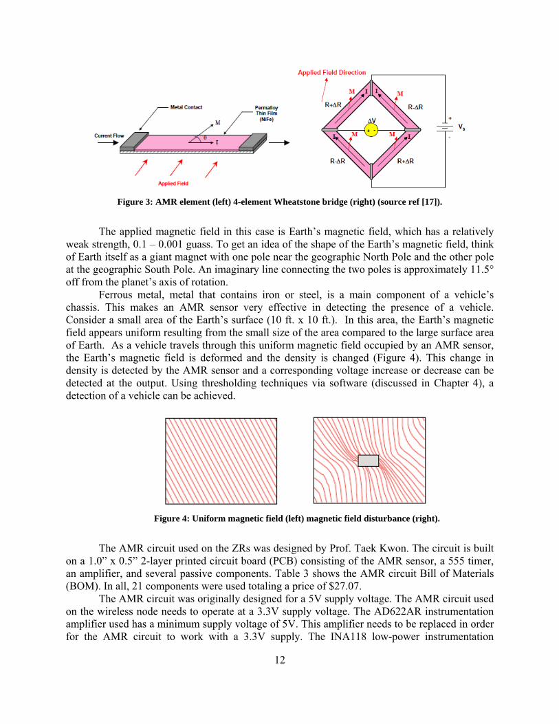
Anisotropic magnetoresistance occurs in ferrous materials and can be applied as a thin strip to become a resistive element. The AMR sensor used, HMC1001, manufactured by Honeywell, uses a ferrous material called Permalloy (nickel-iron) and forms four resistive elements to become a 4-element Wheatstone bridge sensor. Each magnetoresistive strip element possesses an ability to change resistance in a cos2θ relationship where θ is the angle between the magnetic moment (M) vector and the current flow (I) [17]. Figure 3 shows the Permalloy element with field and current applied as well as the 4-element Wheatstone bridge.

In the presence of an applied magnetic field, a change in the bridge resistance causes a corresponding change in output voltage. When an external magnetic field applied normal to the side of the film causes the magnetization vector to rotate and change θ. This in turn will cause the resistance value to vary and produce a voltage output (Vs) change in the Wheatstone bridge. This change in the Permalloy resistance is termed the magnetoresistive effect. The Permalloy element in the HMC1001 is capable of detecting magnetic fields as low as 30 µguass with a sensitivity of 3.2 mV/V/gauss [18].

12

Figure 3: AMR element (left) 4-element Wheatstone bridge (right) (source ref [17]).

The applied magnetic field in this case is Earth’s magnetic field, which has a relatively

weak strength, 0.1 – 0.001 guass. To get an idea of the shape of the Earth’s magnetic field, think of Earth itself as a giant magnet with one pole near the geographic North Pole and the other pole at the geographic South Pole. An imaginary line connecting the two poles is approximately 11.5° off from the planet’s axis of rotation.

Ferrous metal, metal that contains iron or steel, is a main component of a vehicle’s chassis. This makes an AMR sensor very effective in detecting the presence of a vehicle. Consider a small area of the Earth’s surface (10 ft. x 10 ft.). In this area, the Earth’s magnetic field appears uniform resulting from the small size of the area compared to the large surface area of Earth. As a vehicle travels through this uniform magnetic field occupied by an AMR sensor, the Earth’s magnetic field is deformed and the density is changed (Figure 4). This change in density is detected by the AMR sensor and a corresponding voltage increase or decrease can be detected at the output. Using thresholding techniques via software (discussed in Chapter 4), a detection of a vehicle can be achieved.

Figure 4: Uniform magnetic field (left) magnetic field disturbance (right).

The AMR circuit used on the ZRs was designed by Prof. Taek Kwon. The circuit is built on a 1.0” x 0.5” 2-layer printed circuit board (PCB) consisting of the AMR sensor, a 555 timer, an amplifier, and several passive components. Table 3 shows the AMR circuit Bill of Materials (BOM). In all, 21 components were used totaling a price of $27.07. The AMR circuit was originally designed for a 5V supply voltage. The AMR circuit used on the wireless node needs to operate at a 3.3V supply voltage. The AD622AR instrumentation amplifier used has a minimum supply voltage of 5V. This amplifier needs to be replaced in order for the AMR circuit to work with a 3.3V supply. The INA118 low-power instrumentation

13

amplifier, manufactured by Burr-Brown ($8.43), was used in its place. This amplifier has a minimum supply voltage of 2.7V and is specifically designed for low-power, battery operated devices. All other components meet the specification for a 3.3V supply voltage.

Since a different instrumentation amplifier is being used in the AMR circuit, the gain of the amplifier had to be adjusted. Originally, the AMR circuit using the AD622 amplifier was designed for a gain of 118 with RG = 430Ω in the following gain equation:

1 (50.5 / )GGain k R= + (1)

This gain proved to be too small when the INA118 amplifier and a 3.3V supply voltage is used. The gain was changed to 199 using a 255Ω resistor. Also, to increase the sensitivity of the AMR sensor, the position of the HMC1001 was changed. Originally, the HMC1001 was positioned to lay flat on the PCB. To expose the entire sensor to the Earth’s uniform magnetic field and thus increase sensitivity, the HMC1001 was positioned to extend vertically above the PCB.

Table 3: AMR Circuit Bill of Materials Quantity Reference Package Description Manufacturer Part Number Cost

1 U1 SOIC-8 555 Type, Timer/Oscillator (Single) Texas Instruments

TLC555CD

$0.68

1 U2 SOIC-8 Instrumentation Amplifier Analog Devices AD622AR

$6.95

1 U3 SIP-8 Linear Magnetic 1 Axis Sensor Honeywell HMC1001

$17.00

1 Q1 SOIC-8 MOSFET, N/P-CH, 30V, 4.1/3.4A

Fairchild Semiconductor

FDS8333C

$0.21

1 D1 SOD-123 Diode Switch 100V On Semiconductor

MMSD4148T1G

$0.42

1 R1 SMD603 1.0kΩ, 1/16W, 5% tolerance resistor Panasonic ERA-3YEB102V $0.16 1 R2 SMD603 330kΩ, 1/16W, 5% tolerance resistor Susumu Co Ltd RR0816P-334-D $0.14 1 R3 SMD603 24kΩ, 1/16W, 5% tolerance resistor Panasonic ERA-3YEB243V $0.16 1 R4 SMD603 432Ω, 1/16W, 1% tolerance resistor Panasonic ERA-3YEB431V $0.16 2 R5, R6 SMD603 51kΩ, 1/16W, 5% tolerance resistor Susumu Co Ltd RR0816P-513-D $0.14 6 C1,C2,C4,

C5, C7,C9

SMD603 0.1uF, 16V, 10% tolerance ceramic capacitor

Yageo

06032R104K7B20D

$0.11

1 C3 SMD603 0.01uF, 50V, 10% tolerance ceramic capacitor

Murata

GRM188R71H103KA01D

$0.04


Venkel X7R160224KNE

$0.04

2 C8, C10 SMD805 4.7uF, 10V, 10% tolerance ceramic capacitor

Kemet C475K8PACTU

$0.17

When manufactured, the HMC1001 preferred direction of magnetic field is set to one

direction along the length of the Permalloy resistive strip. This allows the maximum change in resistance for an applied magnetic field. However, the influence of a strong magnetic field of 10 guass or more along this axis could upset, or flip, the polarity of film magnetization, thus changing the sensor characteristics. Following such an upset field, a strong restoring magnetic field must be applied momentarily to restore, or set, the sensor characteristics. A combination of the 555 timer and the MOSFET transistor applies a 215kHz, 0.5A, 2µs pulse to the Set/Reset pin of the HMC1001. This pulse realigns the magnetic domains of the Permalloy strip to one direction to ensure high sensitivity and repeatable readings.

14

3.2 Panasonic PAN4570 Module The Panasonic PAN4570 module is one of the first products to employ Ember’s EM250 ZigBee SoC technology. The PAN4570 module contains the single chip EM250 from Ember Inc., a 24MHz reference crystal, chip antenna, and RF front-end circuitry optimized for best RF performance. The PAN4570 is packaged in a 48-pin quad flats no (QFN) leads and its dimensions are 20mm x 26.5mm x 3.0mm. Figure 5 shows the PAN4570 module.

Figure 5: PAN4570 module (source ref [19]).

The PAN4570 is powered by a supply voltage in the range of 2.1 – 3.6 VDC applied on

the VBAT pin. In order to program the PAN4570 module, an Ember Insight Adapter is required. The PAN4570 contains a Serial Programming Interface; known as a SIF, to facilitate the software programming and debugging of the EM250 chip. SIF is a synchronous port which operates in a similar command/response manner as JTAG connections. The SIF is accessed by the Insight Adapter through a 10-pin header, manufactured by Samtec, connected to the PAN4570 module. Table 4 describes the 10 pins used for programming and debugging software in the PAN4570 module.

Table 4: Description of Used PAN4570 Pins

Pin No. Pin Name Pin Type Description 1 VBAT Input Module DC supply voltage 3 RESET Input Reset of the module 10 PTI_EN Output Frame Signal of Packet Trace Interface (PTI) 11 PTI_DATA Output Data Signal of PTI 13 GND Input/Output Ground 25 SIF_CLK Input Serial Interface, clock 26 SIF_MISO Output Serial Interface, master in/slave out 27 SIF_MOSI Input Serial Interface, master out/slave in 28 SIF_LOADB Input/Output Serial Interface, load strobe A 10kΩ pull-down resistor is attached to pin 27, SIF_MOSI, in order to tie it to ground

and achieve the low quiescent current specified in Chapter 12 of the PAN4570 datasheet [19].

15

In addition to the 10 pins used for programming the PAN4570 module, two additional pins are used as inputs. Pin 14, General Purpose Input/Output (GPIO) 7, of the PAN4570 module is used as an input to the analog-to-digital (ADC) converter. The output of the AMR circuit is connected to this pin. The software functionality of the ADC is described in Chapter 4. Pin 21, GPIO14, of the PAN4570 module is connected to a 511Ω resistor and a red LED. When the PAN4570 module is transmitting or receiving, GPIO14 goes high, turning on the LED.

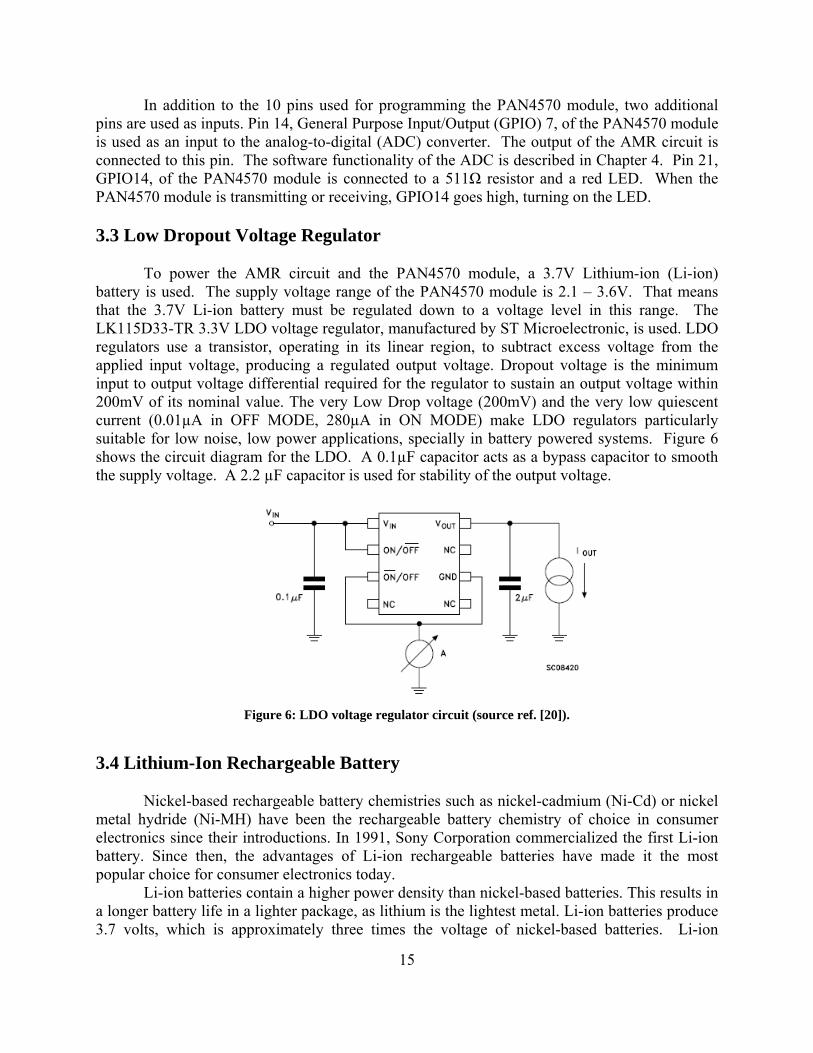
3.3 Low Dropout Voltage Regulator

To power the AMR circuit and the PAN4570 module, a 3.7V Lithium-ion (Li-ion) battery is used. The supply voltage range of the PAN4570 module is 2.1 – 3.6V. That means that the 3.7V Li-ion battery must be regulated down to a voltage level in this range. The LK115D33-TR 3.3V LDO voltage regulator, manufactured by ST Microelectronic, is used. LDO regulators use a transistor, operating in its linear region, to subtract excess voltage from the applied input voltage, producing a regulated output voltage. Dropout voltage is the minimum input to output voltage differential required for the regulator to sustain an output voltage within 200mV of its nominal value. The very Low Drop voltage (200mV) and the very low quiescent current (0.01µA in OFF MODE, 280µA in ON MODE) make LDO regulators particularly suitable for low noise, low power applications, specially in battery powered systems. Figure 6 shows the circuit diagram for the LDO. A 0.1µF capacitor acts as a bypass capacitor to smooth the supply voltage. A 2.2 µF capacitor is used for stability of the output voltage.

Figure 6: LDO voltage regulator circuit (source ref. [20]).

3.4 Lithium-Ion Rechargeable Battery Nickel-based rechargeable battery chemistries such as nickel-cadmium (Ni-Cd) or nickel metal hydride (Ni-MH) have been the rechargeable battery chemistry of choice in consumer electronics since their introductions. In 1991, Sony Corporation commercialized the first Li-ion battery. Since then, the advantages of Li-ion rechargeable batteries have made it the most popular choice for consumer electronics today. Li-ion batteries contain a higher power density than nickel-based batteries. This results in a longer battery life in a lighter package, as lithium is the lightest metal. Li-ion batteries produce 3.7 volts, which is approximately three times the voltage of nickel-based batteries. Li-ion

16

batteries have none of the memory effects that are seen in Ni-Cd batteries. Memory effect is the phenomenon where the apparent discharge capacity of a battery is reduced when it is repetitively discharged incompletely and then recharged. This allows recharging of a Li-ion battery whenever convenient, without the full charge or discharge cycle necessary to keep nickel-based batteries at peak performance. Finally, Li-ion batteries have a lower self discharge rate than nickel-based batteries. Nickel based batteries can lose anywhere from 1-5% of their charge per day (depending on the storage temperature) even if they are not connected to a load. Li-ion batteries can hold most of their charge even after months of storage. One disadvantage of Li-ion batteries is that the life span of the battery is dependent upon time of manufacturing regardless if the battery was charged. Also, Li-ion batteries are one of the most expensive battery chemistries on the market. The battery selected to power a ZR is the 3.7V Li-ion battery manufactured by UltraLife. This battery has a capacity of 950mAh. Battery capacity and size are directly related; the larger the capacity the larger the physical size of the battery. This battery was selected because of its small size (1.42” x 2.13” x 0.24”), which aides with the requirement of a small footprint each ZR must have. But more importantly, the capacity is large enough to support the power requirements of a ZR. There are two components on the ZR that consume power; the AMR sensor and the PAN4570 module. The AMR draws a steady state current of 8mA. When the PAN4570 is transmitting or receiving data, the current draw is 35.5mA. The total current consumption of a ZR is the addition of the current draw of these two devices: 43.5mA. The life of the battery (BL) in hours is then: ( ) _ / _ 950 / 43.5 21.8hoursBL Battery Capacity Current Draw mAh mA hours= = = (2)

This means that if the wireless node is continuously detecting a vehicle and transmitting

or receiving data, the battery would last 21.8 hours. In an actual intersection, traffic usually peaks for a 2 or 3 hour period in the morning and afternoon corresponding with people traveling to and from work. The rest of the time, specifically late evening and early morning, intersection occupancy is very low. The wireless node would remain mostly idle during these low traffic times. As a result, a battery capacity of 950mAh is more than enough to support a wireless node for several days under normal traffic conditions.

The battery leads are connected to a female, rectangular housing using crimp contacts. Attached to the wireless node and the battery charger circuit is a male, through-hole, 3-pin header. This allows the battery to be easily connected and disconnected from either the wireless node or the battery charger circuit (Section 3.8).

3.5 PADS Software

The five components mentioned above: AMR sensor, PAN4570 module, 3.3V LDO voltage regulator, Li-ion rechargeable battery and connector, and the Samtec 10-pin header are all needed to build a prototype wireless node. To build a prototype wireless node, several circuit design steps need to be completed. First, logic schematic and layout files are created using Mentor Graphics PADS software. Next, the layout file is imported into a PCB manufacturing editor, LPKF CircuitCAM PCB software. From CircuitCAM, a LPKF S62 prototyping machine is used to create the physical prototypes of the wireless node.

17

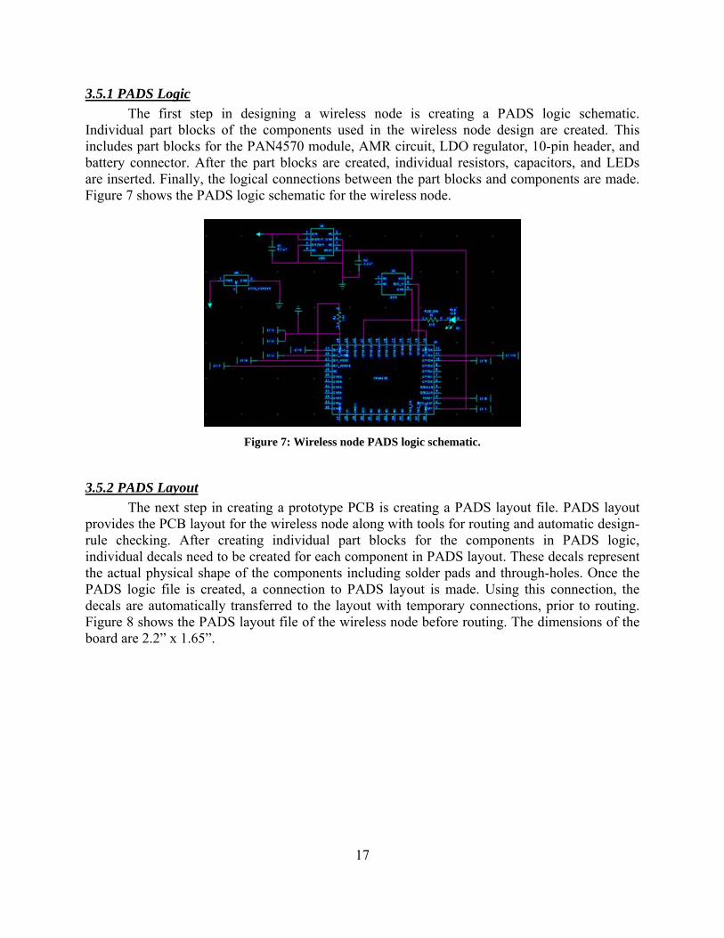
3.5.1 PADS Logic The first step in designing a wireless node is creating a PADS logic schematic.

Individual part blocks of the components used in the wireless node design are created. This includes part blocks for the PAN4570 module, AMR circuit, LDO regulator, 10-pin header, and battery connector. After the part blocks are created, individual resistors, capacitors, and LEDs are inserted. Finally, the logical connections between the part blocks and components are made. Figure 7 shows the PADS logic schematic for the wireless node.

Figure 7: Wireless node PADS logic schematic.

3.5.2 PADS Layout The next step in creating a prototype PCB is creating a PADS layout file. PADS layout

provides the PCB layout for the wireless node along with tools for routing and automatic design-rule checking. After creating individual part blocks for the components in PADS logic, individual decals need to be created for each component in PADS layout. These decals represent the actual physical shape of the components including solder pads and through-holes. Once the PADS logic file is created, a connection to PADS layout is made. Using this connection, the decals are automatically transferred to the layout with temporary connections, prior to routing. Figure 8 shows the PADS layout file of the wireless node before routing. The dimensions of the board are 2.2” x 1.65”.

18

Figure 8: Wireless node PADS layout before routing.

After setting the design-rules for minimum distance between pads, vias, through-holes,

and traces; a built-in auto-router tool in PADS layout can be used to automatically create the routes. After the auto-routing is complete, individual routes can be edited, moving traces to different positions and layers. PADS layout supports multi-layer boards. In the wireless node, only two layers are used, so routes and components can be present on either the top or bottom layer of the PCB. In the design of the wireless node, all components are located on the top layer. This is because the battery must be placed flat against the backside of the wireless node. Since all components are on the top layer, routing can be very difficult. Vias are used to help with simplifying the routing process. A via is a pad with plated hole that connects the copper traces from one layer of a board to another. Figure 9 shows the PADS layout file of the wireless node after routing. The red traces are located on the top layer. The blue traces are located on the bottom layer.

Figure 9: Wireless node PADS layout after routing.

3.6 Wireless Node Prototype

After the routing is completed in the PADS layout file, there is one more software program that needs to be used to prepare the PCB for the manufacturing.

19

3.6.1 CircuitCAM CircuitCAM is a PCB software package created by LPKF to aid in the manufacturing of

PCBs. This software processes the same data that would be sent to a PCB manufacturer. Once a design is created in PADS layout, Gerber files need to be created and imported into CircuitCAM. Gerber files are a standard file format used by PCB fabrication machines that contain information necessary for computer controlled machines to draw exact patterns for circuit boards. From PADS layout, seven Gerber files need to be created: Top.pho, Bottom.pho, Plated.drl, Unplated.drl, Silkscreen.pho, PasteMaskTop.pho, and PasteMaskBottom.pho. The Top.pho and Bottom.pho files are images of the top and bottom layers including pads, through-holes, vias, and routes. The Plated.drl file contains locations of holes that need to be through-hole plated such as vias. The Unplated.drl file conations the locations of holes that do not need to be through-hole plated such as mounting holes. The Silkscreen.pho is an image of the names and outlines of the components on the top layer. The PasteMaskTop.pho, and PasteMaskBottom.pho are images of the only the solder pads of top and bottom layers. The solder pads are where component pins will be hand soldered after the PCB is created.

After these seven files are imported into CircuitCAM, there are a few tasks that need to be completed. First, insulating of both the top and bottom layers need to be completed. Insulating is done around terminals, pads, traces, and vias in order to separate them from the copper layer on the board. Next, the board cut-out and breakout tabs are created. This allows the PCB to be removed from the copper sheet. Finally, mounting holes and copper rubout can be added if needed. Figure 10 shows the completed wireless node CircuitCAM file.

Figure 10: Wireless node CircuitCAM file.

3.6.2 LPKF ProtoMat S62 Plotter After the CircuitCAM file has been created, it needs to be exported to an .lmd file. This

file is used by the LPKF ProtoMat S62 plotter. The LPKF ProtoMat S62 is a circuit board plotter for in-house rapid PCB prototyping. This plotter provides the ability for quickly and easily milling and drilling circuit board prototypes in a single day. The LPKF ProtoMat S62 can mill and drill all types of PCBs with extremely fine traces, with a precision as fine as 0.25µm. Its main features include a 10-position tool changer that automatically replaces milling and drilling tools while the board is being produced. This significantly reduces setup time, and allows for

20

unattended operation. In-house PCB prototyping eliminates production delays and the high cost of outside vendors, reducing a product's development time.

3.6.3 LPKF ProConduct and LPKF ProMask After the PCB is milled and drilled on the LPKF ProtoMat S62 plotter, the next step is to

through-hole plate the vias defined in the Plated.drl file. The LPKF ProConduct system produces conductive through-holes without chemical electroplating tanks or potentially hazardous chemical processing. The LPKF ProConduct uses a conductive polymer to quickly and easily plate vias in just a few minutes. This four-step process lends itself well to parallel processing and results in smoothly plated through-holes in a fraction of the time and cost of chemical electroplating. The LPKF ProConduct system plates vias as small as 0.4mm in diameter. The basic process requires only a few minutes for double-sided boards. The electrical resistance of LPKF ProConduct results in extremely low – approximately 19.2mΩ, depending on the material thickness.

The final step in creating a PCB prototype is creating the solder mask using the LPKF ProMask finish. The LPKF ProMask is a cost-effective solution for producing professionally masked PCBs in an in-house prototyping environment. The LPKF ProMask is an easy-to-apply green solder resist mask. This professional finish, ideal for all rapid PCB projects, is especially important for Surface Mount Technology (SMT) projects where traces are very close and circuit isolation and insulation are critical. The LPKF ProMask finishes prototype PCBs professionally and helps protect traces and prevent short circuits from soldering conventional though-hole or SMT components.

3.6.4 Final Wireless Node Prototype After several designs and prototypes, a final wireless node was created. Figure 11 shows

a photo of the final wireless node prototype. The dimensions of the wireless node are 2 3/16” x 1 5/8”. All the components were hand soldered. A 2” braided-wire antenna was added at the base of the supplied chip antenna on the PAN4570 module to improve the wireless range.

21

Figure 11: Wireless node prototype.

3.6.5 Wireless Node Bill of Materials Table 5 shows the wireless node BOM. In all, 11 components were used totaling a price

of $74.05. Originally, a RCM from Ember was considered being used for the wireless nodes. This RCM alone costs $109 to purchase from Ember. Using the LPKF ProtoMat S62 proved beneficial in both the ability to customize the design of the wireless node as well as reduces the total cost of a wireless node.

Table 5: Wireless Node Bill of Materials

Quantity Reference Package Description Manufacturer Part Number Cost 1 U1 48-pin

QFN PAN4570 2.4GHz ZigBee Ember Module w/ chip antenna

Panasonic ENW-C9A02A3E $34.52

1 U2 NA Anisotropic Magnetoresistive (AMR) Sensor

Milwaukee Electronics

NA $27.07

1 U3 SOIC-8 3.3V LDO Regulator ST Microelectronic

LK115D00 series $1.01

1 U4 3-pin Through-hole, side-mount 3-pin header (Male)

JST S3B-PH-K-S(LF)(SN)

$0.11

Rectangular Housing (Female) JST PHR-3 $0.04 Crimp Contacts JST SPH-002T-P0.5S $0.03

1 NA 24 AWG 3.7V (950mAH) Lithium-Ion Rechargeable Battery

UltraLife UBP053450/PCM $8.72

1 J1 SMD 10-pin Header for connecting Insight Adapter

Samtec FTSH-105-01-FDVK

$1.56


Murata GRM series $0.15


Murata GRM series $0.35

1 D1 SMD1206 Red LED Lumex SML-LX1206IW-TR

$0.28

1 R1 SMD1206 510Ω, 1/4 W, 5% tolerance resistor Panasonic ERJ-8GEYJ511 $0.09 1 R2 SMD1206 10k Ω, 1/4W, 5% tolerance resistor Panasonic ERJ-8GEYJ103 $0.09

22

3.7 Wireless Router Prototype In order to extend the range of the WMSN, wireless routers are needed. If a wireless node is out of the range of the ZC, placing an intermediate router in between the ZC and the out of range node will allow messages to and from that node to be routed through the router. This allows the WMSN to be scalable, adding wireless router nodes along the edge of the network range in order to increase the distance the network can reach. This is the main feature of the proposed WMSN for vehicle tracking that differentiates it from the commercially available Sensys Networks Inc.’s vehicle sensing system. Distances between the ZC and the ZRs deployed in an intersection can vary depending on the location of the ZC and the positions of the ZRs. To assure that all wireless nodes whose responsibility is to detect vehicles are within range of the ZC, separate wireless routers were built. These wireless routers contain all the components of a wireless node except for the AMR circuit. Therefore, they do not contain vehicle detection functionality. The only responsibility of a router node is to be part of the network and help route messages between a ZC and other ZRs. Figure 12 shows a photo of a wireless router.

Figure 12: Wireless router prototype.

Since there is no AMR circuit, the size of the wireless router is much smaller than a wireless node. The dimensions of the wireless router are 1 1/8” x 1 5/8”. The absence of the AMR circuit also reduces the cost to build a wireless router, which is $46.98. 3.8 Battery Charger Circuit

When the battery voltage level becomes low, a method of recharging the battery is needed. In order to recharge a battery, a separate battery charger circuit was built. The bq24002 single-cell Li-ion charge management IC manufactured by Texas Instruments was chosen as the device to control the charging of the batteries. This device combines high accuracy current and

23

voltage regulation, battery conditioning and temperature monitoring, charge termination, charge-status indication, and a charge timer into a 20-lead Thin Shrink Small-Outline Package (TSSOP) PowerPad (PWP). The bq24002 measures battery temperature using an external thermistor. The bq24002 then charges the battery in three phases: preconditioning, constant current, and constant voltage. If the battery voltage is below the internal low-voltage threshold, the bq24002 uses low-current precharge to condition the battery. A preconditioning timer is provided for additional safety. Following preconditioning, the bq24002 applies a constant-charge current to the battery. An external sense-resistor (RSNS) sets the magnitude of the current. The constant-current phase is maintained until the battery reaches the charge-regulation voltage. The bq24002 then transitions to the constant voltage phase. The accuracy of the voltage regulation is better than ±1% over the operating junction temperature and supply voltage range. Charge is terminated by maximum time or minimum taper current detection. The bq24002 automatically restarts the charge if the battery voltage falls below an internal recharge threshold.

Figure 13: Li-ion battery charger circuit (source ref. [21]).

Figure 13 shows the circuit diagram of the battery charger circuit. The first step in

designing the battery charger circuit is to design the temperature sensing circuit. The bq24002 continuously monitors temperature by measuring the voltage between the adapter power good/thermistor (APG/THERM) pin and ground. For temperature, a negative-temperature coefficient thermistor (NTC) and an external voltage divider develop this voltage. The following equations are used to calculate the values of the resistors (RT1 and RT2) in the voltage divider.

24

First calculate RT2:

RT2 =

1 1

1 1

B H CC H

B BH C

H C

V R RV V

V VR RV V

⎡ ⎤−⎢ ⎥

⎣ ⎦⎛ ⎞⎛ ⎞

− − −⎜ ⎟⎜ ⎟⎝ ⎠ ⎝ ⎠

(3)

Then use the resistor value of RT2 to calculate RT1:

RT1 = 1

1 12

B

C

C

VV

RT R

−

+ (4)

where: VB = VCR (bias voltage) = 2.85V [21] RH = resistance of the thermistor at the desired hot trip threshold = 4.917kΩ (Table 6) RC = resistance of the thermistor at the desired cold trip threshold = 27.219kΩ (Table 6) VH = lower APG trip threshold = 0.558V [21] VC = upper APG trip threshold = 1.498V [21] RT1 = top resistor in the divider string RT2 = bottom resistor in the divider string

The normal charging temperatures for the Li-ion battery should be in the range of 0° - 45° C (32° - 113° F). Charging out of this temperature range is harmful to the Li-ion battery and must be avoided. If the battery temperature is outside this range, the temperature sensing circuit will detect this and enter a thermal shutdown and suspend charging until the battery temperature returns within the normal charging temperature range. Using these ends values of temperature and the temperature characteristics of the thermistor in Table 6, resistances of the thermistor at the desired hot (RH) and cold (RC) trip thresholds can be found.

25

Table 6: Temperature Characteristics of the NTC Thermistor (source ref. [21])

Using the values found above, RT2 and RT1 can be calculated.

RT2 = ( )( )( ) 1 12.85 4.917 27.219

1.498 0.5582.85 2.854.917 1 27.219 1

0.558 1.498

V k kV V

V Vk kV V

⎡ ⎤Ω Ω −⎢ ⎥⎣ ⎦⎛ ⎞ ⎛ ⎞Ω − − Ω −⎜ ⎟ ⎜ ⎟⎝ ⎠ ⎝ ⎠

= 98.217kΩ (5)

RT1 =

2.85 11.498

1 198.217 27.219

VV

k k

−

+Ω Ω

= 19.245kΩ (6)

The second step in designing the battery charger circuit is to design the current regulation

circuit. The bq24002 provides current regulation while the battery-pack voltage is less than the regulation voltage. The current regulation loop effectively amplifies the error between a reference signal, ViLIMIT, and the drop across the external sense resistor, RSNS. Charge current feedback, applied through pin ISNS, maintains regulation around a threshold of ViLIMIT. The following formula calculates the value of the sense resistor:

RSNS = ViLIMIT / IREG (7) where: IREG = 950mA ViLIMIT = 0.1V [21]

26

RSNS = 0.1V / 950mA = 0.105Ω (8)

The bq24002 continues with the charge cycle until termination by one of the two possible termination conditions; maximum charge time or minimum current. The bq24002 sets the maximum charge time through pin TMRSEL. The TMRSEL pin allows the user to select between three different total charge-time timers (3, 5, or 6 hours). In this battery charger circuit, the TMRSEL pin is left floating with a 10pF capacitor to set the charge-time timer to 3 hours. The charge timer is initiated after the preconditioning phase of the charge and is reset at the beginning of a new charge cycle. In the case of a thermal shutdown, the bq24002 suspends the timer. The bq24002 monitors the charging current during the voltage regulation phase. The bq24002 initiates a 22-minute timer once the current falls below the trip threshold. Fast charge is terminated once the 22-minute timer expires. The bq24002 incorporates two LEDs (red and yellow) for charge status display. Table 7 summarizes the operation of the LEDs.

Table 7: LED Status (source ref. [21])

Charge State Stat1 (Red LED) Stat2 (Yellow LED) Pre-charge ON (LOW) OFF Fast Charge ON (LOW) OFF Fault Flashing (1Hz, 50% duty cycle) OFF Done (>90%) OFF ON (LOW) Sleep-mode OFF OFF APG/Therm invalid OFF OFF Thermal Shutdown OFF OFF Battery Absent OFF OFF

3.8.1 Final Battery Charger Circuit The battery charger circuit was designed and built using PADS logic, PADS layout,

CircuitCAM, and LPKF ProtoMat S62 plotter in the same method as the wireless node prototype. Figure 14 shows the final battery charger circuit with the Li-ion rechargeable battery. All the components were hand soldered. The battery is connected underneath the charger. The battery is recharged using power supplied by a 5V AC/DC wall transformer. A 50% discharged 3.7V battery takes approximately 3 hours to fully charge to 4.2V. The completion of a recharge is signified by the yellow LED turning on.

27

Figure 14: Battery charger circuit and li-ion rechargeable battery.

3.8.2 Battery Charger Circuit Bill of Materials For a total of $9.14, a battery charger circuit can be built. This cost does not include the

price of the AC/DC wall transformer, which is $7.16. There are a total of 16 components in the battery charger circuit that were all hand soldered. Table 8 shows the battery charger circuit BOM.

Table 8: Battery Charger Circuit Bill of Materials

Quantity Reference Package Description Manufacturer Part Number Cost 1 U1 20-

HTSSOP Single Cell Li-Ion Charge Management IC

Texas Instruments

BQ24002PWP $3.60

1 D3 SMD1206 Yellow LED Lumex SML-LX1206SYC-TR

$0.66

1 D2 SMD1206 Red LED Lumex SML-LX1206IW-TR $0.28 1 U3 3-pin Through-hole, side-mount 3-pin

header (Male) JST S3B-PH-K-

S(LF)(SN) $0.11

1 R1 SMD1206 0.1Ω, 1/4W, 5% tolerance resistor

Panasonic ERJ-L08KJ10CV $0.77

2 R2, R3 SMD1206 510Ω, 1/4W, 5% tolerance resistor

Panasonic ERJ-8GEYJ511 $0.09

1 R5 SMD1206 RT1, 19.1kΩ, 1/4W, 1% tolerance resistor

Panasonic ERJ-8ENF1912V $0.12

1 R6 SMD1206 RT2, 97.6kΩ, 1/4W, 1% tolerance resistor

Panasonic ERJ-8ENF9762V $0.12

1 R4 Molded Bead

10kΩ, NTC Thermistor Murata NTSD1XH103FPB30

$0.59

1 C5 SMD1206 10pF, 50V, 5% tolerance ceramic capacitor

AVX 12065A100JAT2A $0.42


Murata GRM31CR71H105KA16L

$0.15


Murata GRM31CR71H105KA61L

$0.45

1 C1 SMD1206 10uF, 25V, 10% tolerance ceramic capacitor

Murata GRM31CR61E106KA12L

$1.02


Panasonic ECJ-3YB1H224K $0.23

1 NA NA 5V DC @ 1.0A AC/DC Wall Transformer, 12mm long plug

CUI Inc. EPS050100-P6P $7.16

1 U2 4-Contact SMD

16V DC @ 2.5A, 2.1mm ID, 5.5mm OD Male Jack

CUI Inc. PJ-002A-SMT $0.81

28

3.9 Wireless Node Housing

An important part of the wireless node hardware is its housing. The six wireless nodes used in this vehicle tracking system must be placed in the middle of traffic lanes in order to detect vehicles. This exposes the nodes to the chance of getting run over by a vehicle. In order to protect the wireless node circuitry, it must be housed in a strong, durable, and low-profile enclosure. The wireless node housing shape is modeled after a raised pavement marker. Raised pavement markers are commonly used as a safety device on roads, usually contain reflective material, and are made from plastic. The housings used to protect the wireless nodes are made from fiberglass. Fiberglass was the material chosen because of its strong composition and will not interfere with the detection of vehicles or the transmitting and receiving of the wireless nodes. Fiberglass housings were purchased from a company in Milwaukee, Wisconsin. These housings came as solid pieces and needed to be milled in order for the wireless node to fit inside. The dimensions of the housing are 4 ¾” x 4 ¾” x 1”. The sides of the housing are angled. Using a JET milling machine, a 2 3/8” x 1 7/8” x 9/16” space was milled out from the bottom of the housing in order to place the wireless node inside. A 3/8” x 1/4” x 1/8” and a 1/8” x 1/2” x 1/8” hole were milled out for the 10-pin header and HMC1001 components because they extend beyond the PCB. These holes assure a tight fit of the wireless node in the housing, minimize the removal of material from the housing, and help to maximize the housing strength. A 1/8” diameter hole was drilled to through the top of the housing for the antenna. The antenna extends 1.5” above the top of the housing so a 1/8” x 1 ½” slit was milled on the top of the housing so the antenna can be positioned against the housing and is not sticking straight up. Also, a 1” x 3/8” x ¼” slit was milled on the bottom of the housing from one edge. This slit is used for prying the housing off the pavement after it has been installed. Complete dimensions of the housing can be seen in Figure 15.

29

Figure 15: Top, bottom, front, and side views of the wireless node housing.

Installing the housings in the traffic lane requires very little time. First, the battery needs

to be connected to the wireless node. A piece of foam is then placed inside the housing to cushion the wireless node’s components from the fiberglass. The wireless node and battery are then placed inside the housing and another piece of foam is placed on top. A piece of black duct tape is placed over the wireless node and battery to hold it in the housing. Then a multipurpose adhesive spray manufactured by 3M is sprayed on the bottom of the housing as well as the location in the roadway where the wireless node is to be placed. The housing is firmly placed on the roadway. The drying time of the adhesive is approximately 30 seconds. The housings are painted black in order to blend in with the asphalt. This helps to hide the wireless node from the driver’s of vehicles to facilitate normal driving through the intersection where the WMSN is deployed. Figure 16 shows images of the actual wireless node housing and Figure 17 shows a wireless node placed inside a sensor housing.

30

Figure 16: Wireless node housing.

Figure 17: Wireless node inside a sensor housing.

31

CHAPTER 4: NODE SOFTWARE DESIGN

Included in the Ember EM250 development kit is the EmberZNet 3.0 software package.

Released in January 2007, EmberZNet is a complete ZigBee protocol software package containing all the elements required creating mesh networking applications on Ember’s EM250 SoC. EmberZNet offers the ability for developers to customize peripherals such as ADC, Universal Asynchronous Receiver/Transmitter (UART), and GPIO available on the EM250 SoC through the Hardware Abstraction Layer (HAL). Larger networks potentially consisting of thousands of nodes in a single network are enabled by stochastic addressing, multicast, broadcast, and many-to-one routing, and asymmetric link handling. Denser networks are enabled by Ember’s intelligent table management system that assures network stability even when many routing nodes are within close proximity. More secure networks are enabled by implementing many of the optional ZigBee security extensions for advanced network encryption and device security. These features are all included in the source code and will not be discussed in detail. For further information on these topics, please refer to [10, 23].

Included with the development kit is xIDE, a development environment for the EM250. xIDE provides a compiler and debugger that can be used to program the XAP2b microprocessor on the EM250 SoC using the C/C++ language. EmberZNet includes several sample projects for the EM250 that can be used to start custom applications. The provided sink/sensor application is an example application that shows how a single device collects data from multiple devices. This application was used as the base for creating the software for the ZC and ZRs in this vehicle tracking system. There are two separately compiled application workspaces, sink and sensor. The sink application will run on the ZC node. The sensor application will run on the six ZR nodes. Each application runs a similar main program loop shown in Figure 18.

Figure 18: Main event loop (source ref. [10]).

32

In the Initialization state, the serial ports and HAL are initialized, interrupts are turned on, and a request for reset is checked. If the node was already a member of an existing network, it then joins that network if present. The event loop is then entered. First, the watchdog timer is reset. The watchdog timer is a hardware timing device that triggers a system reset if the main event loop encounters a fault. If the watchdog timer is not reset every 2 seconds, a reset of the device will occur. Next, the function emberTick() is called. Here, any pending ZigBee stack work is done. This includes managing input and output stack buffers and processing any stack callbacks. If the device’s network state is “joined” then the function processSerialInput() is called. Here, the device monitors the serial port. Characters can be sent to a device through either the Insight Desktop or a Hyper Terminal connection. Depending on what characters are read by the device, specific tasks are executed. Next, the function applicationTick() is called. Here, services are provided for the application such as checking for timeouts, control inputs, and changing any indicators (like an LED). If the device is not “joined” to a network and it is a ZC, it will form a network. If the device is not “joined” to a network and it is a ZR, it will then try to rejoin an existing network or attempt to join a new network if one is present. In both cases, the processSerialInput() and applicationTick() functions are passed over until a device has created or joined a network. In the function applicationTick(), software functionality was added in order to customize the source code for a vehicle tracking WMSN.

The added functionality of the ZC includes updating its address table, synchronizing the local clocks of the ZRs, receiving vehicle detection messages from the ZRs, and forwarding this data through a serial port connection. The added functionality of the ZRs are to continuously calculate a moving average based on the static level of the AMR sensor, sample the ADC and recognize a vehicle detection, sending a timestamp when a vehicle detection occurs, and acknowledging the ZC when a “sink advertise” message is received. The following sections will describe this added software functionality.

4.1 Sink Advertise

Once a ZC is powered on, it scans the 16 available channels on the 2.45GHz band, finds a clear channel, and establishes a network. In the ZC applicationTick() function, a “sink advertise” multicast message is sent out over the selected network channel. This message is used to identify ZRs that wish to join the network. When a ZR requests to join a network and is allowed, the ZC adds the ZR to its address table. Each ZR contains a unique 64-bit extended unique identifier (EUI). This EUI is stored in the ZC address table along with its associated index, inuse boolean value, node ID, and age. Table 9 shows an example of a ZC address table with 4 ZRs joined to the network.

33

Table 9: ZC Address Table

Index Inuse Node ID EUI64 Age 00 TRUE 0x0AC7 11 7F 0A 00 00 6F 0D 00 0x000D 01 TRUE 0x2F00 1E AA 0A 00 00 6F 0D 00 0x000D 02 TRUE 0x6D77 1A AA 0A 00 00 6F 0D 00 0x000C 03 TRUE 0x0864 50 7F 0A 00 00 6F 0D 00 0x000C 04 FALSE UNUSED FF FF FF FF FF FF FF FF 0xFFFF 05 FALSE UNUSED FF FF FF FF FF FF FF FF 0xFFFF 06 FALSE UNUSED FF FF FF FF FF FF FF FF 0xFFFF 07 FALSE UNUSED FF FF FF FF FF FF FF FF 0xFFFF 08 FALSE UNUSED FF FF FF FF FF FF FF FF 0xFFFF 09 FALSE UNUSED FF FF FF FF FF FF FF FF 0xFFFF 10 FALSE UNUSED FF FF FF FF FF FF FF FF 0xFFFF

The index of each ZR refers to the location in the address table. The number of ZRs in an

address table depends on the maximum number of children a parent is allowed to have and the maximum number of routers that can be children. These values are set by the ZC upon formation of the network. The node ID of a ZR is just a short 16-bit ID the ZC assigns to each ZR when added to the network. The Inuse column identifies the ZR as being either active (TRUE) or inactive (FALSE). This inactivity depends on the age of each node. Every time a ZR sends any kind of message (alive, clock synchronization, or vehicle detection) to the ZC, its age is reset to zero. If the ZC hasn’t received a message from a ZR for more than 5 minutes, its age reaches its maximum value of 0xFFFF and it is considered inactive (Inuse = FALSE). The ZR must request to rejoin the network after it becomes inactive.

To keep each ZRs status as active, a ZC sends a multicast “sink advertise” message every 60 seconds. When a ZR receives a “sink advertise” message, it responds with an “alive” message. This allows the ZC to reset the age of each ZR and keep them active. If a ZR powers down or is out of range, it will not be able to respond the “sink advertise” message, its inuse value will be set to FALSE, and it must request to rejoin the network when powered back up or returns within range. A ZC will ignore its own multicast “sink advertise” message.

4.2 Clock Synchronization

Clock synchronization is an integral part of this vehicle tracking system. When a wireless

node detects a vehicle, it sends its node EUI along with a timestamp of when the detection occurred. The vehicle tracking algorithm then uses the position of the nodes along with the timestamps of each detection to accurately track vehicles through an intersection. The timestamp is derived from the physical clock of a wireless node and can differ from node to node. This difference in physical clocks can be a result of when each node was powered on, clock skew, or clock jitter. If there is a single wireless node in WMSN whose clock is not synchronized with the rest of the nodes, the vehicle tracking algorithm will not be as effective as when all wireless nodes are synched. The Mock et al. clock synchronization protocol [24] is used in this vehicle tracking WMSN.

34

4.2.1 Mock et al. Clock Synchronization Protocol The Mock et al. clock synchronization protocol exploits the broadcast property of the

master (ZC) by assuming that message reception between master and slaves (ZRs) is tight. If two slaves receive the same message, it can be assumed that they receive it at approximately the same time. Based on this property, the time-critical path is shown in Figure 19.

Figure 19: Mock et al. timing diagram (source ref. [24]).

The time-critical path is the path of a message that contributes to non-deterministic errors

in the protocol. Usually, non-deterministic errors of clock synchronization include the send, access, and propagation times. The send time is the time from the master clock reading to the sending of the broadcast message. The access time is the time between slaves receiving the broadcast message and adjusting their local clocks. The propagation time is the time between the broadcast message being sent and when the slaves receive the message. The propagation time is usually much smaller than both the send and access times. Because the Mock et al. protocol utilizes the broadcast property in wireless networks, the send and access times can be eliminated from the time-critical path. Therefore, the time-critical path in the Mock et al. protocol is the time between t3 to tS, or the propagation time. The protocol uses two messages for synchronization between a master and a group of slaves, a multicast indication message followed by a multicast confirmation message. The main steps in the synchronization protocol of Mock et al. are shown below.

• The master prepares an indication message (t1) and broadcasts it (t2). • The message is delivered to a number of slave nodes with negligible delay, assuming

tight message reception. • Each slave and the master receive the message (t3) and take a local timestamp (tS). • The master sends its own timestamp in the confirmation broadcast message (t5). • Each slave compares the master timestamp with its own timestamp for the reception of

the last indication message, computes the difference t5 − t3, and adjusts its local clock (t6).

In the Mock et al. protocol, continuous clock synchronization is used by implementing a rate-based algorithm to either speed up or slow down the virtual clock. Instead of continuous clock synchronization, instantaneous clock synchronization is used in the in the WMSN. In the case of instantaneous clock synchronization, a slave computes a local clock error and adjusts its clock using this computation. This results in abrupt changes in local clock time, which can cause

35

time discontinuity. Time discontinuity can lead to serious faults in distributed systems, such as a slave missing important events. Continuous clock synchronization avoids such discrepancies by spreading the correction over a finite interval. Since each slave in the WMSN only uses its local clock to assign a timestamp to a vehicle detection and not to trigger events, continuous clock synchronization is not needed.

The local clock of a slave is its physical clock. The physical clock consists of an oscillator, whose frequency is fixed. The physical clock can not be adjusted in any way. A virtual clock uses a function that transforms physical clock values to virtual clock values. A virtual clock is intended to correct the skew rate of the physical clock of the slave such that it resembles the physical clock of the master. Here, the virtual clock is calculated at t6 by adding a clock offset to the physical clock value. The clock offset is calculated by computing the difference t5 − t3. The goal is to match the virtual clock of a slave to the physical clock of the master as closely as possible.

4.2.2 Mock et al. Examples There are two different cases that the Mock et al. protocol must handle. The first is when

the ZC is powered on before a ZR. This means that the ZC’s physical clock (5000ms) will have a higher value than the ZR’s physical clock (3000). Figure 20 illustrates this example using the Mock et al. clock synchronization protocol.

ZC ZRZC Physical Clock = 5000ms ZR Physical Clock = 3000ms

Transmit data = 0

Save ZR Physical ClockZR Physical Clock = 3010ms

Save ZC Physical Clock ZC Physical Clock = 5010ms

TX = 0

TX = 0

TX = 5010

Clock Offset = ZC Physical Clock – ZR Physical Clock = 5010 – 3010 = 2000ms

ZR Virtual Clock = Physical Clock + Clock Offset = 3000 + 2000 = 5000ms

Transmit data = 5010

Figure 20: Mock et al. clock synchronization protocol, example 1. The ZC initiates the protocol by sending a multicast indication message containing data =

0. This indication message is received by both the ZC and the ZRs joined to the network after 10ms (the worst case latency for 1 hop). When a ZR receives this indication message with the data = 0, it saves its physical clock value (3010ms) at that time. When the ZC receives its own indication message with a data = 0, it transmits a multicast confirmation message containing its physical clock value at the time of the reception of the indication message (5010ms). When the

36

ZR receives this confirmation multicast message, it calculates the difference between the ZC physical clock and its own physical clock (5010ms – 3010ms). This difference equals the value of the clock offset (2000ms). This clock offset value is then added to its physical clock (2000ms + 3000ms), matching the physical clock of the ZC (5000ms). A ZC will ignore the confirmation message.

The second case is when a ZC is powered on after a ZR. This means that the ZC’s physical clock will have a lower value than the ZR’s physical clock. Figure 21 illustrates this example using the Mock et al. clock synchronization protocol. The difference is that the clock offset value will now be negative.

ZC ZR

ZC Physical Clock = 1000ms ZR Physical Clock = 3000ms

Transmit data = 0

Save ZR Physical ClockZR Physical Clock = 3010ms

Save ZC Physical Clock ZC Physical Clock = 1010ms

TX = 0

TX = 0

TX = 1010

Clock Offset = ZC Physical Clock – ZR Physical Clock = 1010 – 3010 = -2000ms

ZR Virtual Clock = Physical Clock + Clock Offset = 3000 + (-2000) = 1000ms

Transmit data = 1010

Figure 21: Mock et al. clock synchronization protocol, example 2.

4.3 Simple Moving Average

The AMR circuit produces an analog output voltage signal depending on the strength of the Earth’s magnetic field surrounding the sensor. When the AMR circuit is present in a uniform magnetic field, there is an associated “static level” analog output voltage signal depending on the strength of the uniform magnetic field. This static level continually changes by a few millivolts, even if the sensor is stationary. It also changes if the sensor is moved just a few feet, and is different from sensor to sensor. If the static level of every AMR circuit was identical, a global threshold could be used to determine if a vehicle was detected. If the AMR output voltage increased or decreased above or below this threshold, vehicle detection would occur. But because of this changing static level, the threshold has to change along with the static level. This is done using a simple moving average (SMA) for the static level.

SMA works as follows. At any time t, the algorithm first averages a sequence of samples (k) , 1 ,,...,i t k i tx x− + at each sensor i, and gets:

, 1 ,( ... ) /i t k i tx x x k− += + + (9)

37

The oldest sample, , 1i t kx − + , is replaced by a new sample ,i tx at every time t. In each ZR, the sample size k = 10 and the sample set is updated every second.

The SMA is only used in ZRs. When a ZR is powered on, a 30 second initialization period is used to set the SMA. During this initialization period, the ZR should be stationary in its intended position in the intersection. The ZR is not allowed to detect vehicles during this time. Once the SMA is set, it is continuously updates every second (1 Hz) in the applicationTick() function. If a vehicle is about to be detected, the static level of the AMR circuit will increase or decrease. This change in the static level due to a vehicle detection should not be part of the SMA. To assure this, another sample of the AMR circuit is taken at 100Hz. If a value of this 100Hz sample is above the threshold, the next SMA value will be skipped until the AMR circuit output voltage falls back underneath the threshold.

Figure 22: Simple moving average example.

Figure 22 shows an example of an output signal (red) from the AMR circuit. When the

output signal voltage level is between the threshold values, the SMA is updated every 1 Hz. After four updates, the 100Hz ADC sample detects the output voltage signal level above the threshold. The next value of the SMA value is skipped. The SMA update is skipped a total of four times because the ADC sample either detects the AMR sensor voltage to be above or below the threshold value. When the ADC sample detects that the AMR signal level has fallen back with the threshold range, the SMA is allowed to update itself again.

4.4 Sampling the Analog-to-Digital Converter

The AMR circuit produces an analog output voltage signal depending on the strength of the Earth’s magnetic field that surrounds the sensor. To work with this signal in software it must be digitized. The GPIO7 pin on the PAN4570 is used to convert the analog signal to a numbered value. The resolution of the ADC is set for 12-bits. The number of quantization levels for the ADC with a 12-bit resolution is:

122 4096Quantization Levels levels = = (10)

38

The output of the AMR sensor has a voltage range from 0 – 1.2V. The voltage resolution is then: 1.2 0 ) / 4096 mV/levelVoltage Resolution V V level = ( − = 0.29 (11)

After the 30 second initialization period of the SMA, a ZR is allowed to sample the ADC input every 100Hz in the applicationTick() function. Once a sample is taken, it is subtracted from the SMA and the absolute value of the result is computed. The absolute value is taken because a vehicle can be detected by either being above the threshold (SMA + threshold) or below the threshold (SMA – threshold). This is illustrated in Figure 20. The threshold value selected for each ZR is 500 levels. The corresponding voltage threshold is then:

levels x 0.29mv/level =145mVVoltage Threshold = 500 (12)

If the AMR circuit output voltage is 145mV above or below the SMA, a vehicle detection will occur. To eliminate noise, there must be three successive vehicle detections before an actual vehicle detection occurs. Once this happens, a timestamp of when the detection occurs is recorded. This timestamp is the value of the physical clock plus the value of the clock offset configured in the clock synchronization protocol (Section 4.2). The physical clock is a 32-bit number that increments every one millisecond. The physical clock will not overflow for almost 5 days. The ZR will send a unicast message to the ZC with the timestamp as its data. Also, to assure that a vehicle hovering over a sensor or a slow moving vehicle is not detected more than once, the ADC must read 100 consecutive samples within the threshold range after a vehicle detection before another vehicle detection can occur.

4.5 Logging of Vehicle Detections

The ZC is responsible for logging vehicle detection data. When a ZC receives a vehicle detection message from a ZR, it writes a comma separated line of data to the serial port. An example of a line of data written to the serial port after vehicle detection data is received from a ZR is *,000D6F00000A7F11,0000032450.

The asterisk (*) designates that this is vehicle detection data. The first number is the ZRs EUI. The second number is the timestamp, in milliseconds, of when the vehicle detection occurred. A Real-time Data Collector (RtDC) graphical user interface (GUI) was coded using Visual Basic in Microsoft Visual Studio.NET 2005 to log vehicle detections. The ZC development board has a RS-232 interface which is connected to a laptop computer by a serial cable. The laptop runs the RtDC GUI (Figure 23).

39

Figure 23: Real-time data collector GUI.

First, the COM port of the laptop that is connected to the ZC must be selected and

opened. To receive a list of ZRs that are connected to the network, the “Update Active Nodes” button is pressed. The ZC responds to the button press by sending a list of the active nodes in its address table. The list is a comma separated line starting with the pound (#) character. This is so the RtDC can distinguish between vehicle detection data (*) and an active node list (#). These are the only types of data that the RtDC will display from the ZC. The user has the option of recording a start time of data collection. When data collection is finished, the user can record a stop time. The vehicle detection data that was collected is logged in a text file. The name of the text file is the date when data collection occurred. Figure 24 shows an example of data that was collected on October 4, 2008.

Figure 24: Vehicle detection data collected on 10/4/08.

This logged data is then used by the vehicle tracking algorithms to provide an accurate

trajectory count of the direction of vehicles through an intersection. The details of the vehicle tracking algorithm are discussed is Chapter 6.

40

4.6 Debugging and Testing Serial Port Commands

Along with the software functionality added to the sink and sensor workspaces mentioned in this chapter, there are several serial port commands that the sink application uses for debugging and testing the wireless nodes. These commands can be sent to the ZC through a serial port connection using either the Insight Desktop or a Hyper Terminal application. If the command “Rxx” is written to the serial port, the ZC coordinator will send a unicast message requesting the device at the xx location in its address table to reset itself. By writing the command “Txx0100” to the serial port of the ZC will send a unicast message requesting the device at the xx location to change its global threshold value to 100. The device will respond with a unicast message sent back to the ZC containing its present SMA value. The command “Hxx0010” will send a unicast message requesting the device change the number of successive ADC samples above or below the threshold before an actual vehicle detection occurs to 10. The command “Zxx0200” will send a unicast message to the device requesting it to change the number of consecutive samples in the threshold range to 200.

4.6.1 Over-the-Air Passthrough Bootloading Over-the-Air (OTA) bootloading is a way to upload source code wirelessly from a ZC to

a device that is connected to a network. When using OTA passthrough bootloading, the source node (ZC) is connected to a PC via a serial cable. The uploaded source code originates from the PC, which sends the source code to a network device over a serial line and then passes the source code to the target node over the air. The source of OTA passthrough bootloading must be within range of the ZC and within one hop.

Figure 25: Over-the-air passthrough bootloading (source ref. [10]).

The source device uses a simplified MAC-based protocol to communicate with the target.

This protocol is based on XModem CRC but uses 64-byte data blocks that can fit in a single IEEE 802.15.4 packet. During OTA upload, only the target device actually runs the bootloader. The source device and any intermediary devices that participate in the upload process continue to run an application. Figure 25 illustrates the OTA passthrough bootloading process.

41

CHAPTER 5: INTERSECTION SIMULATOR

Before we do any actual testing of the WMSN in an intersection, the vehicle tracking

algorithm needs to be tested. A software simulation of an intersection has been created using Visual Basic programming language in Microsoft Visual Studio.NET 2005 environment. This intersection simulation allows a real intersection to be recreated and vehicle movements through the intersection to be simulated. The movements of vehicles through the intersection will produce logged data that is similar to the logged data of the actual WMSN. This logged data can then be used by the vehicle tracking algorithm to verify that the algorithm is tracking vehicles correctly before any actual data is collected. Along with verifying that the vehicle tracking algorithm works, the intersection simulator will help us determine the minimum number of nodes that need to be deployed in an intersection, as well as the position of each node.

A single lane T-intersection has been chosen as the configuration of the intersection where data will be collected. This configuration was chosen to simplify the intersection simulator, tracking algorithms, and collection of real-time data. Once we have verified that vehicle movements through a T-intersection can be successfully tracked, the system can be expanded to more difficult intersection configurations.

5.1 Cellular Division of an Intersection

To obtain spatial traffic information from a WMSN, a cellular approach is used. The intersection is divided into individual cells in which wireless nodes could be placed. The dimensions of the cells are designed based on the spatial resolution needs of the WMSN. Each wireless node contains a wireless node including an AMR sensor that detects disturbances by vehicles in the Earth’s magnetic field. The range of the AMR sensor is about 3 feet. This means that an AMR sensor needs to be driven over by a vehicle for a detection to occur. If a vehicle were to pass by an AMR sensor more than 3 feet away from the sensor, it would not be detected. This small range will not allow a wireless node to detect a vehicle traveling in an adjacent lane. Wireless nodes can then be placed in the middle of traffic lanes and are allowed to be side by side in adjacent lanes.

Figure 26 shows two examples of a cellular division of an intersection. The width of the cells in these two images are 12’ x 12’. These dimensions were chosen because the width of a traffic lane in Minnesota is 12’ [25]. Having a much larger width of a cell compared to the range of an AMR sensor (3 feet) assures that if sensors are placed in neighboring cells, a single vehicle will not be detected by more than one sensor.

42

Figure 26: Current (left) and original (right) intersection cellular configuration.

The first image (left) is the current configuration of position and number of nodes used

for vehicle tracking in a T-intersection. There are a total of six nodes, one for each traffic lane. Each node is placed in a cell one cell away from the middle of the intersection. In an actual intersection, each traffic lane is defined by a white boundary line on the right side of the lane and a dashed yellow line on the left side of the lane. These lines give the driver of a vehicle a limited space in which to drive. The space in the middle of an actual intersection does not contain any boundary lines. Depending on the driver of the vehicle, the trajectory of a vehicle through the middle of an intersection can differ slightly from vehicle to vehicle. If a node were to be placed in the middle of the boundary lines, there is a good chance that it might be run over by a vehicle.

The second image (right) was the original configuration of nodes. There are a total of 12 nodes. After developing the tracking algorithms, it was concluded that this configuration contains an excess amount of nodes. The same tracking algorithm results could be obtained by reducing the number of nodes from 12 to 6. Not only could the tracking algorithms be simplified, but the reduction in the number of nodes reduced the time to build the prototypes as well as reduced the testing time.

5.2 Intersection Simulator Design In Figure 26 (left) there are three entrance nodes (nodes 1, 4, and 5) and three exit nodes (nodes 2, 3, and 6). A vehicle can then travel through the intersection on six different trajectories. These trajectories are North-to-East (NE), North-to-West (NW), East-to-West (EW), East-to-North (EN), West-to-East (EW), and West-to-North (WN). Table 10 summarizes the entrance and exit nodes associated with each trajectory.

43

Table 10: Trajectory Entrance and Exit Nodes

Entrance Node Exit Node Trajectory Node 1 Node 3 NW Node 1 Node 6 NE Node 4 Node 2 WN Node 4 Node 6 WE Node 5 Node 2 EN Node 5 Node 3 EW

The intersection simulator GUI is shown in Figure 27. The six nodes in the intersection need to be assigned EUIs. A node can be assigned a EUI by either drag-and-dropping EUIs from the Active Node list or by pressing the “Automatic Assign” button. The intersection is represented by a 19x12 array. Vehicles are represented by red squares. Vehicle trajectories can be simulated in two ways, by pressing individual trajectory buttons or by starting a random simulation.

Figure 27: Intersection simulator GUI.

When an individual trajectory button is pressed, a vehicle is placed in the intersection array in the cell at the start of the corresponding entrance lane. The vehicle square is drawn, erased, and moved to the next cell. This process is repeated until the vehicle has moved through all cells on its trajectory. As a vehicle passes through a cell that contains a node, that node’s EUI and a timestamp in milliseconds is recorded in the “Recorded Data” textbox. The timestamp value is calculated from the system clock. This data is also written to a text file. The name of the text file is the date when the simulated data was collected. The text file is identical to the logged data collected in Section 4.5 and shown in Figure 24.

The second way to record simulated intersection data is to start a random simulation. This random simulation uses a shifted negative exponential (SNE) distribution function [26] to calculate headway distribution between vehicles. The vehicle-per-hour (VPH) values can be changed by the user before a simulation is started and should be specific to the actual intersection

44

that is being simulated. The random simulation generates and logs data in the same fashion as describe above. During a random simulation, the number of nodes that generated a vehicle detection and the total number of tracks that were simulated are recorded. Also, a table keeps track of the 6 individual trajectory counts as well as the headway between vehicle releases calculated by the SNE distribution function.

5.2.1 Shifted Negative Exponential Distribution Function At the outset of a simulation run, the intersection array is empty. Vehicles are generated

at entrance points according to a SNE distribution function based on VPH volumes. The SNE distribution will yield the following expression: min minh ln(1-R)] + H hh = (Η − )[− − (13) where: h = headway (seconds) separating vehicle emissions H = mean headway = 3600/VPH hmin = specified minimum headway (seconds) R = random number in the range 0–1.0

The SNE distribution function is commonly used for low-volume, single-lane headway calculations. This distribution is based on the assumption that vehicles arrive at random without any dependence on the time the previous vehicle arrived and that there is a minimum headway between vehicles, hmin. A possible range of headways is calculated using the SNE. The value selected in this range depends on the VPH and the random number, R, generated by a pseudo-random number generator. A larger VPH value results in a smaller calculated headway. A larger random number results in a larger calculated headway.

45

CHAPTER 6: VEHICLE TRACKING ALGORITHM

The tracking algorithm used in the WMSN for vehicle tracking in an intersection uses a

form of multiple target tracking (MTT). MTT, a discipline first developed in 1955, is essential for surveillance systems employing multiple sensors, together with a computer subsystem, to interpret an environment [27]. Typical sensor systems in MTT include radar, infrared, and sonar. The MTT objective is to partition the sensor data into sets of observations, or tracks, produced by the same source. Once tracks are formed and confirmed, the number of targets can be estimated and target velocity, future predicted position, and target classification can be computed for each track. Originally developed for military applications such as radar, air-to-air and air-to-land defense, and battlefield intelligence, MTT has made its way into commercial applications due technology advances allowing cost-effective wireless sensor networks to be deployed.

MTT incorporates a discipline called multisensor data fusion. Multisensor data fusion attempts to combine data from multiple sensors to perform inferences that may not be possible from a single sensor [28]. Data fusion is analogous to the cognitive process used by humans to integrate data continuously from their senses to make inferences about the external world. Humans receive and process data from their five senses – sight, sound, smell, touch, and taste – which are then assessed to draw conclusions about the environment.

6.1 Elements of a Multiple Target Tracking System

Figure 28 shows a block diagram of a simple recursive MTT system. There are five elements that represent this system: sensor data processing, gating equations, correlation, track initiation, confirmation, and deletion, and filtering and prediction.

Figure 28: MTT block diagram (source ref. [27]).

First, input data is received from a node. This input data is often preprocessed before

being passed to the gating equations. Pre-processing is specific to individual nodes and data types. Examples of pre-processing include image processing, signal processing, and filtering. Next, gating is used to decide if an observation belongs to a previously established track or to a new target track. If an observation satisfies the gate of one more existing tracks, it becomes a candidate to be associated with that track. Note that more than one observation may satisfy the gate of a single track. Also note that an observation that satisfies the gate of an existing track might not be used to update that track. In this case the observation will be a candidate for the

46

initiation of a new target track. Next, the correlation function takes the output of the gating function and makes a final observation-to-track assignment. In the case where a single observation is within the gate of a single track, the association can be made immediately. However, for closely spaced targets, a correlation conflict arises when multiple observations fall within the same gate and when observations fall within the gates of multiple tracks. Observations not associated to an existing track are used to form new tentative tracks. Once a tentative track is formed, it is usually required that at least one other observation be associated to the tentative track before the track is confirmed. A track that is not updated is deleted. The final step is the filtering and prediction function. After the inclusion of the new observations, tracks are predicted ahead of the arrival time for the next set of observations. Gates are placed around these predicted positions and the MTT processing cycle repeats. 6.2 Modified Multiple Target Tracking System

There are few differences between the MTT systems described above and the one that is used in the presented vehicle tracking system. The first is that MTT tracks real-time targets. Target tracks are updated as a target moves through the area occupied by the node network. As a node detects a target, it uses gating functions to associate it to an existing track or to create a tentative new target track. The proposed vehicle tracking algorithm tracks vehicles through an intersection using logged data. This logged data is a compilation of all vehicle detections resulting from vehicles that traveled through the intersection in a specific period of time. Second, the correlation function in MTT is broken into two separate functions: Track Initiation and Track Association. These two functions are entered according to what type a node (entrance or exit) was outputted from the Gating Function. Finally, MTT uses filtering and prediction to create gating functions that predict the next move of a target. In MTT, a target can travel anywhere in the node field. Filtering and prediction is usually done using a Kalman filter [29]. The proposed vehicle tracking algorithm does not use any filtering or prediction functions. Once a vehicle has entered the intersection it has only two options for leaving the intersection. With such a small range of options, predicting a vehicles path is not necessary.

Figure 29 shows the modified MTT system used in the development of the vehicle tracking algorithm. Each block is discussed in detail in the following sections.

Figure 29: Modified MTT block diagram for the vehicle tracking algorithm.

47

6.2.1 Logged Vehicle Detections Vehicle detections are recorded by each node in a WMSN. Magnetic field disturbances

around a wireless node are converted from an analog signal to a digital signal. Three successive detections above or below the threshold offset verify that a vehicle is present. After a vehicle is detected, the wireless node sends its EUI and a timestamp of when the detection occurred. The ZC of the WMSN receives this detection data from all nodes in the WMSN. When vehicle detection data is received, the ZC writes the source of the detection along with the timestamp into a text file. This text file is a log file containing all the vehicle detections from a WMSN over an arbitrary time period. Figure 24 shows an example of a log file.

The vehicle tracking algorithm reads the data from the log file and places each line of the text file into an array list. Vehicle detections are not guaranteed to be logged in order they were detected. When a vehicle detection occurs, it is time stamped and sent to the ZC. Because of routing and that failed messages are retried, a vehicle detection of a node that occurred after a vehicle detection on another node might reach the ZC first. The array list that each line of the text file is stored in must be sorted according to each line’s timestamp. Each item of the list array is then split into a two-dimensional string array. The first item in the string array is the 16-bit node EUI. The second item is the 32-bit timestamp in milliseconds. The string array is then passed to the gating function of the vehicle tracking algorithm. This process is repeated until every line of the logged data has been placed in an array list, split, and sent to the gating function.

6.2.2 Gating and Track Initiation When actual data is being collected in an intersection, the position and EUI of each node

in the WMSN must be recorded. When the vehicle tracking algorithm reads through the data of the log file, it records and lists the EUIs of all wireless nodes that produced vehicle detections. Before the vehicle tracking algorithm can began, each EUI listed must be dragged-and-dropped to its corresponding node position on the vehicle tracking GUI (Figure 30).

The gating function compares the node EUI of each string array it receives to the entrance and exit nodes of the intersection. Nodes 1, 4, and 5 are entrance nodes. Nodes 2, 3, and 6 are exit nodes. As a vehicle passes through the intersection, it travels over one entrance node and one exit node. If the node EUI is an entrance node, a new track is initiated. Tracks are stored in Current Track array and contain the node EUI and timestamp of each node. Both incomplete and complete tracks are stored in the array list. A count of the current number of tracks is recorded. The gating function is then re-entered and the next line of data from the logged data text file is read. If the node EUI is an exit node, the string array is then passed to the Track Association function.

48

Figure 30: Vehicle tracking GUI.

6.2.3 Track Association The goal of this function is to associate an exit node with its corresponding entrance

node, i.e. complete a track. In the Track Association function, the array of tracks is looped through until an incomplete track is found that contains an entrance node that the exit node could be assigned to. For example, exit node 2 could be assigned to an incomplete track if the entrance node in that track is either node 5 (East – North trajectory) or node 4 (West – North Trajectory). If the timestamp of the entrance node is smaller than the timestamp of the exit node, the exit node is associated with that track. If the timestamp of the entrance node is greater than or equal to the exit node, the entrance node produced a vehicle detection after the exit node, which cannot be considered a valid track. In this case, this track is skipped and the next incomplete track that is valid is searched for.

When an entrance node is associated to a track, it is also kept in Last Node Added array that stores the last node associated to a track. This is because there are certain cases where the tracking algorithm fails to associate the correct exit node with an entrance node. When one of these cases occurs, an association error is encountered. An association error is when there are one or more incomplete tracks but the exit node is not a valid association to the entrance nodes. Figure 31 illustrates this association error.

49

Figure 31: Example of an association error and solution.

The next node that enters the Track Association function is Node 6, 72986. The only

track in the Current Track array that is incomplete is track 137. The entrance node to this track is node 5. The association node is exit node 6. It is not possible for a track to have an entrance node of 5 and an exit node of 6. This means that there was an association error in one of the previous completed tracks. To fix the association error, the vehicle tracking algorithm must go back to the last node associated with a track located in the Last Node Added array. The last node associated with a track is Node 3, 72288 (circled in red). This node is deleted from track 136 and the Last Node Added array. The Track Association function is then executed with Node 6, 72986 as the associated node. This node is associated with track 136 and added to the Last Added Node array. The replaced node, Node 3, 72288, becomes the next associated node. It is associated with track 137 and added to the Last Node Added array. The vehicle tracking algorithm continues on with the Gating function. A new entrance node (Node1, 73405) was used to initiate track 138. The next Association Node is Node 6, 74089. This node will be associated with track 138, and the vehicle tracking algorithm continues. If replacing the last node added does not allow the vehicle tracking algorithm to continue, it will try and replace the second to last node added. If this fails, it will replace the third to last node added. Through experimentation, going back a maximum of three added nodes is sufficient to fix any association error.

The vehicle tracking algorithm must also deal with sensors detecting a vehicle more than once. This usually occurs with large vehicles such as five axle trucks or vehicles that are hovering over a sensor while stopped at a stop sign. Section 4.4 discusses software functionality of the wireless nodes that deals with these cases. If an extra vehicle detection occurs on an exit node, a node association will occur where there are no incomplete tracks for this node to be assigned to. In this case, it is added to the Extra Node array and the vehicle tracking algorithm continues. If an extra vehicle detection occurs on an entrance node, the vehicle tracking algorithm cannot determine if this was an error or not, it will always initiate a new track. The result is an incomplete track when the vehicle tracking algorithm completes.

50

After completion of the vehicle tracking algorithm, the completed tracks are looped through, displayed in the Tracks text box, and trajectory counts are recorded and displayed. Also, the number of entrance nodes, the number of exit nodes, and which exit nodes were not associated with a track are displayed in the Tracks text box. Trajectory counts are counted by looking at the entrance and exit nodes of each track and comparing the node EUIs to the position of the nodes arranged on the Vehicle Tracking GUI. If there are incomplete tracks, the vehicle tracking algorithm randomly chooses a trajectory to count depending on the location of the incomplete tracks entrance node. For example, if the incomplete track contains a vehicle detection by node 1, it will randomly choose between either updating the NW or NE trajectory. 6.3 Vehicle Tracking Algorithm Limitations

In some cases, the vehicle tracking algorithm incorrectly associates an exit node with an entrance node. This happens when the two successive trajectories enter the intersection approximately at the same time. Although an incorrect association occurs, the trajectories are still counted correctly. There are a total of three cases where this occurs, summarized in Table 11.

Table 11: Vehicle Tracking Algorithm Incorrect Associations – Correct Trajectories

Successive Trajectories

Tracking Algorithm Association

Tracking Algorithm

Trajectories

Actual Trajectories

Error

EW – NW Track 1 = (EW, NW) Track 2 = (NW, EW)

EW = 1 NW = 1

EW = 1 NW = 1

EW = 0 NW = 0

WN – EN Track 1 = (WN, EN) Track 2 = (EN, WN)

WN = 1 EN = 1

WN = 1 EN = 1

WN = 0 EN = 0

NE – WE Track 1 = (NE, WE) Track 2 = (WE, NE)

NE = 1 WE = 1

NE = 1 WE = 1

NE = 0 WE = 0

Take for example the two successive vehicle trajectories of EW and NW in Table 11. In this case (Figure 32 left), the EW vehicle is traveling ahead of the NW vehicle towards the intersection. The EW vehicle crosses node 5 at 500ms and the NW vehicle crosses node 1 at 550ms. After each vehicle pauses at the stop sign, the EW vehicle crosses its exit node (node 6) at 1,800ms, before the NW vehicle crosses its exit node (node 6) at 2,500ms. In this case, the vehicle tracking algorithm will correctly associate each entrance node with its corresponding exit node and the correct trajectories will be counted. In Figure 32 (right) the EW vehicle is again traveling ahead of the NW vehicle. But the NW vehicle crosses its exit node at 1,800ms, before the EW vehicle crosses its exit node at 2,500ms. When this happens, the vehicle tracking algorithm will make an incorrect association. Even though an incorrect association has occurred, the correct trajectories are counted. Because Track 1’s entrance node is Node 5 and its exit node is Node 6, its trajectory is EW. And Track 2’s entrance node is Node 1 and its exit node is Node 6, its trajectory is NW.

51

Figure 32: Example 1 of a correct association (left) and an incorrect association (right).

The case of an incorrect association but a correct trajectory count happens in two other

closely spaced trajectory combinations listed in Table 11. The similar problem of two successive trajectories reaching the intersection at approximately the same time and the trailing trajectory crosses its exit node before the leading trajectory, causes the incorrect association to happen. Even though there is an incorrect association recorded in the vehicle tracking algorithm, the correct trajectories are counted. Take note that these three cases do not occur if the time between the two successive trajectories is large. In three other cases, the vehicle tracking algorithm incorrectly associates exit nodes with entrance nodes, resulting in a miscount of vehicle trajectories. This occurs when three successive trajectories reach the intersection at approximately the same time. Table 12 summarizes these three cases.

Table 12: Vehicle Tracking Algorithm Incorrect Associations – Incorrect Trajectories

Successive Trajectories

Tracking Algorithm Association

Actual Trajectories

Tracking Algorithm

Trajectories

Error

NE – EW – WN

Track 1 = (NE, EW) Track 2 = (EW, WN) Track 3 = (WN, NE)

NE = 1 NW = 0 EW = 1 EN = 0 WE = 0 WN = 1

NE = 0 NW = 1 EW = 0 EN = 1 WE = 1 WN = 0

NE = -1 NW = +1 EW = -1 EN = +1 WE = +1 WN = -1

WN – NE – EW

Track 1 = (WN, NE) Track 2 = (NE, EW) Track 3 = (EW, WN)

NE = 1 NW = 0 EW = 1 EN = 0 WE = 0 WN = 1

NE = 0 NW = 1 EW = 0 EN = 1 WE = 1 WN = 0

NE = -1 NW = +1 EW = -1 EN = +1 WE = +1 WN = -1

WE – EN – NW

Track 1 = (WE, EN) Track 2 = (EN, NW) Track 3 = (NW, WE)

NE = 0 NW = 1 EW = 0 EN = 1 WE = 1 WN = 0

NE = 1 NW = 0 EW = 1 EN = 0 WE = 0 WN = 1

NE = +1 NW = -1 EW = +1 EN = -1 WE = -1 WN = +1

52

Using the three successive trajectories of NE, EW, and WN in Table 12, Figure 33 illustrates incorrect associations resulting in incorrect trajectory counts. Correct associations occur (left) when the trajectory that reaches the intersection first (NE) crosses its exit node before both the EW and WN trajectories cross their respective ext nodes. In this case, the NE vehicle crosses its entrance node, Node 1, at 500ms. The EW vehicle crosses its entrance node, Node 5, at 550ms and the WN vehicle crosses its entrance node, Node 4, at 700ms. All three vehicles pause at their stop signs and continue on into the intersection. The NE vehicle is the first to travel through the intersection and reach its exit node, Node 6, at 1625ms. Next, the EW vehicle travels through the intersection and reaches its exit node, Node 3, at 1800ms. Finally, the WN vehicle is the last vehicle to travel through the intersection and reaches its exit node, Node 2, at 1900ms. These three trajectories traveled through the intersection in the order they all reached the intersection, resulting in a correct association by the vehicle tracking algorithms. In Figure 33 (right), the NE vehicle is still the first vehicle to cross its entrance node followed by the EW and WN vehicles. But the EW vehicle is the first to travel through the intersection and it reaches its exit node, Node 3, at 1625ms. It is followed by the WN vehicle reaching its exit node, Node 2, at 1875 ms, and the NE vehicle reaching its exit node, Node 6, at 1900ms. Since the vehicle that crossed its entrance node first (NE) does not cross its exit node before the EW or WN vehicles, an incorrect association occurs for all three tracks.

Figure 33: Example 2 of a correct association (left) and an incorrect association (right).

Of the three cases listed in Table 12, two of them (NE – EW – WN, WN – NE – EW) cause the NE, EW, and WN trajectories to not be counted (they should be), causing an error of -1 for each. The NW, EN, and EW are counted, causing an error of +1 for each. The third case, (WE – EN – NW) causes the NE, EW, and WN trajectories to be counted, causing an error of +1 for each. The trajectories of NW, EN, and EW are not counted (they should be), causing an error of -1 for each. Say for example during an intersection simulation or collection of real-time data, the two cases of three successive trajectories NE – EW – WN and WE – EN – NW happen. The vehicle tracking algorithm will cause incorrect associations to occur, but the trajectory count will be accurate because the error for the six trajectories will cancel each other out. The case of incorrect associations and miscounted trajectories occurs in two other trajectory combinations listed in Table 12. These incorrect associations occur when the leading trajectory does not cross its respective exit node before the other two trajectories. Similar to the cases listed in Table 11, these three cases do not occur if the time between the two successive trajectories is large.

53

CHAPTER 7: EXPERIMENTAL RESULTS

This chapter presents two sections of experimental results. First, the vehicle tracking

algorithm was tested using simulated data produced by the intersection simulator. Several sets of simulated data are used to test the accuracy of the vehicle tracking algorithm. The intersection that is used for testing the WMSN for vehicle tracking is a 6-lane T-intersection in Duluth, MN. The two roadways that form this test-site intersection are Wallace Avenue and East 4th Street. This intersection is controlled by stop signs. A T-intersection configuration was chosen for its simplicity. Using average annual daily traffic (AADT) values for each roadway, the intersection simulator can be adjusted to generate similar VPH values in order to replicate the test-site intersection. The AADT values are obtained by placing automatic tube counters at the analysis location for a 24-hour period. Figure 34 shows the test-site intersection.

Figure 34: Test-site intersection of Wallace Avenue and East 4th Street (source ref. [30]).

Second, actual data was collected from the test-site intersection using the WMSN for

vehicle tracking. Six wireless nodes are placed in the intersection and collect vehicle detection data for several different time periods. The vehicle tracking algorithm was then used on this actual data to count the trajectories of the vehicles through the intersection. The results of the vehicle tracking algorithm are compared to trajectory counts acquired by a video camera and hand counted.

7.1 Intersection Simulator Testing

Peak-hour traffic can be calculated from AADT values. Typically, peak hour traffic volumes are approximately 8-11 percent of the AADT values on roadways [31]. 2007 Duluth AADT values for the three legs of the test-site intersection were attained from the Mn/DOT Traffic Forecasting and Analysis website [32]. The AADT of Wallace Avenue is 3650 vehicles

54

per day (VPD). For East 4th Street, the AADT for the west roadway is 5800 VPD and 3600 VPD for the east roadway. To obtain peak-hour values, the following equation must be used:

Peak-hour / 2) 11.0%AADT x = ( (14)

These AADT values are for both lanes of each roadway, so the corresponding AADT value needs to be divided by 2 to get a peak-hour value for each lane of the roadway. Table 13 summarizes the AADT and peak-hour values for each roadway of the test-site intersection.

Table 13: Summary of Test-Site Intersection Roadway ADDT and Peak-Hour Values

Intersection Roadway AADT Peak-Hour Wallace Avenue 3650 200 East 4th Street – West Leg 5200 319 East 4th Street – East Leg 3600 198

In order to model the intersection simulator after the test-site intersection, VPH values for

each trajectory through the intersection need to be calculated. There is no equation to calculate turning trajectories of each lane of the roadway from peak-hour values. Using the assumption that most vehicles (75%) on the east roadway of East 4th Street travel straight through the intersection to the west roadway of East 4th Street towards downtown Duluth, the trajectory East – West than has a VPH count of 149 (198 x 75%). The VPH counts for the remaining trajectories can then be calculated from this value. Table 14 shows the VPH counts for the test-site intersection that will be used for the intersection simulator.

Table 14: Simulated Test-Site Intersection VPH Trajectory Counts

Trajectory VPH North – East 30 North – West 170 East – West 149 East – North 51 West – East 168 West - North 151

These VPH trajectory counts were used in the intersection simulator. Three different simulations were conducted at time periods of 15, 30, and 60 minutes. Table 15 summarizes the results of the intersection simulator. For all three durations, the vehicle tracking algorithm correctly tracked all vehicles through the intersection.

55

Table 15: Vehicle Tracking Algorithm Testing Using Simulated Intersection Data

Duration (minutes)

Trajectory

Simulated Trajectories

Tracking Algorithm

Trajectories

Error

NE 7 7 0 NW 38 38 0 EW 42 42 0 EN 15 15 0 WE 41 41 0

15

WN 36 36 0 Total 179 179 0 (0%)

NE 14 14 0 NW 75 75 0 EW 74 74 0 EN 27 27 0 WE 84 84 0

30

WN 72 72 0 Total 346 346 0 (0%)

NE 27 27 0 NW 157 157 0 EW 144 144 0 EN 49 49 0 WE 167 167 0

60

WN 140 140 0 Total 685 685 0 (0%)

In these time durations, none of the three cases listed in Table 12 occurred, which would

lead to association errors and cause incorrect trajectory counts. Since there were no association errors, the accuracy of the vehicle tracking algorithm is 100%. This 100% accuracy, both in individual trajectories and an overall vehicle count, is a result of the low VPH values. These low values allow the vehicle trajectories to be spaced far apart, not allowing an association error to occur. A better test of the vehicle tracking algorithm would be to increase the VPH values of the intersection simulator, therefore decreasing the space between trajectories, resulting in one or more of the association error cases to occur. In order to increase the VPH values, the VPH for all six trajectories are doubled. Table 16 shows the increased VPH counts that will be used for the intersection simulator.

Table 16: Increased VPH Values

Trajectory VPH North – East 60 North – West 340 East – West 298 East – North 102 West – East 336 West - North 302

56

Again, three different simulations were conducted at time periods of 15, 30, and 60 minutes. Table 17 summarizes the results of the intersection simulator.

Table 17: Vehicle Tracking Algorithm Testing Using Increased VPH Values

Duration (minutes)

Trajectory

Simulated Trajectories

Tracking Algorithm

Trajectories

Error

NE 16 15 -1 NW 84 85 +1 EW 80 79 -1 EN 25 26 +1 WE 80 81 +1

15

WN 70 69 -1 Total 355 355 6 (1.69%)

NE 31 30 -1 NW 169 170 +1 EW 153 152 -1 EN 52 53 +1 WE 157 158 +1

30

WN 144 143 -1 Total 706 706 6 (0.85%)

NE 60 59 -1 NW 339 340 +1 EW 303 302 -1 EN 92 93 +1 WE 310 311 +1

60

WN 293 292 -1 Total 1397 1397 6 (0.43%)

In all three time durations, a similar overall trajectory error occurred. The NE, WE, and WN trajectories were off by -1 each and the NW, EN, and WE trajectories were off by +1 each. This could result from either a single case of the three successive trajectories of NE – EW – WN or WN – NE – EW occurring, or a combination of all three cases in Table 12. Take note that several events of the two successive trajectories listed in Table 11 occurred in all three time durations, but these cases do not result in a miscount of trajectories. Also, even though individual trajectories were miscounted, the overall vehicle count for all three time durations was correct. Overall, the counted trajectory errors generated by the vehicle tracking algorithm for each time duration are very small. In the 15-minute duration, a total of 355 vehicles passed through the intersection. The vehicle tracking algorithm miscounted 6 of these vehicles, which resulted in an error of 1.62%. The time duration was doubled to 30 minutes. A total of 706 vehicles passed through the intersection. Again, the vehicle tracking algorithm miscounted 6 of these vehicles. This error is same as the error for the 15-minute interval, but more than twice as many vehicles were counted. This same error and an increase in vehicles results in a smaller error of 0.85%. Finally, the time duration was doubled once more to 60 minutes. A total of 1397 vehicles passed

57

through the intersection. Again, 6 trajectories were miscounted resulting in a total error of 0.43%. 7.2 Testing at the Real T-Intersection Data collection at the test-site intersection of Wallace Avenue and East 4th Street occurred on October 4, 2008 at 2:24 pm. Figure 35 shows the WMSN layout used to collect data in the test-site intersection. The ZC is shown in blue and the ZRs are shown in red. ZRs are labeled with the last 5 digits of their EUI and the distances from each ZR to the ZC are shown in parenthesis. The ZC was positioned in the grass on the west side of Wallace Avenue. All six ZRs in the intersection are positioned in the second cell away from the middle of the intersection. Notice that the positions of each wireless node are not in the middle of their respective cells. This is because before the nodes were placed in the intersection, vehicle behavior was observed. Vehicles traveling on East 4th Street tend to drive closer to the middle boundary line then the side boundary lines. Therefore, all four ZRs on East 4th Street were placed 3 feet from the middle boundary line. This will give a higher chance of a vehicle passing directly over the sensor, resulting in better vehicle detection data. Also, it was observed that when vehicles are traveling towards the intersection, they stay close to the middle boundary line. When they reach the intersection, they deviate from this position depending if they are going to turn or go straight. To counter this affect, all four sensors were placed on the back edge of their respective cells. It was observed that most vehicles traveling southbound on Wallace Avenue take a right turn to travel west on East 4th Street. When vehicles are making this turn, they tend to hug the white boundary line in anticipation of turning. Therefore, the ZR AAA1E was placed 3 feet from the white side boundary line to increase the number of vehicles that travel directly over the nodes.

Figure 35: Test-site intersection WMSN layout.

58

Figure 34 also shows the presence of one wireless router, AAA15, in the WMSN layout. This wireless router was need because the two ZRs on the east leg of East 4th Street, A7F11 and AAA11, were out of the range of the ZC. It was determined that the distance between the ZC and the two ZRs (96 and 102 feet) was greater then the range of the network. The wireless router was placed just off the sidewalk on the north-east corner of the intersection. This wireless router helped extend the range of the ZC in the east direction, allowing messages to be routed to and from the ZC and the two ZRs. The four other nodes in the WMSN were within the range of the ZC. Figure 36 shows an image of myself placing a node in the east bound lane of East 4th Street. Figure 37 shows an image of two deployed sensors on East 4th Street.

Figure 36: Deploying a wireless node in the test-site intersection.

59

Figure 37: Two deployed wireless nodes in the test-site intersection.

After all ZRs were deployed and verified that they were working properly and data logging of vehicle detections could begin. A laptop computer running the RtDC was connected to the ZC via a serial cable. All vehicle detection data collected from the WMSN was written in a text file. There were two sets of vehicle detection data collected. The first was a 30 minute time period from 2:46 pm to 3:16 pm. The second was a 15 minute time period from 3:18 pm to 3:33 pm. A video camera was set up north of the west leg of East 4th Street to record the vehicles traveling through the intersection. The video would be viewed at a later time so vehicle trajectories could be hand counted and compared to the results of the vehicle tracking algorithms. Table 18 summarizes the results of observed trajectories hand counted using the video camera and the results of the tracking algorithm.

60

Table 18: Vehicle Tracking Results Using Original Test-Site Intersection Data

Duration (minutes)

Trajectory

Observed Trajectories

Tracking Algorithm

Trajectories

Error

NE 1 6 +5 NW 25 28 +3 EW 7 7 0 EN 2 2 0 WE 20 19 -1

15

WN 24 25 +1 Total 79 87 10 (12.7%)

NE 6 10 +4 NW 46 46 0 EW 12 17 +5 EN 9 7 -2 WE 44 42 -2

30

WN 42 45 +3 Total 159 167 16 (10.1%)

For the 15 minute time duration, a total of 79 vehicles were observed with the video camera. The vehicle tracking algorithm counted a total of 87 trajectories. Of these 87 trajectories, there were 10 miscounted trajectories compared to the observed, resulting in an error of 12.7%. This error was calculated by dividing the observed total vehicle counted by the number of miscounted trajectories. For the 30 minute time duration, a total to 159 vehicles were observed using the video camera. A total of 167 trajectories were counted by the tracking algorithm. There were a total of 16 miscounted trajectories, resulting in an error of 10.1%. The main reason the vehicle tracking algorithm produces error is incorrect vehicle detections. The incorrect vehicle detections can be caused by four scenarios. First, if a vehicle was not detected when it traveled over an entrance node or an exit node. Second, a vehicle was detected more than once when it traveled over a single node. Third, if a node detected a vehicle when there was not one present. Finally, a vehicle that cuts a corner and travels over an exit node instead of the intended exit node can cause two entrance nodes detections and not the intended one entrance node and one exit node detection. While observing the video and the logged data simultaneously, it was noted that vehicles traveling in the WN trajectory have the tendency to severely cut the corner. When a vehicle cuts this corner, they were detected by the AAA1E node and not the AA948 node. This happened 5 times in the 15 minute data collection duration and 4 times in the 30 minute data collection duration. When this happens, the NW vehicle then travels over two entrance nodes, instead of one entrance node and one exit node. The tracking algorithm has the ability to determine if there was an extra exit node detection but not if there was an extra entrance node detection. This limitation will cause an excess in the total number of vehicles counted by the tracking algorithm. This is evident when comparing the total vehicle counts for both the observed and tracking algorithm trajectories in Table 18. Also, by detecting extra entrance nodes, incorrect associations of exit nodes to their entrance nodes can occur later on in the vehicle tracking algorithm,

61

resulting in a miscount of trajectories in the final totals. Figure 38 shows an example of a NW trajectory cutting the corner.

AAA1E

Figure 38: NW trajectory cutting the corner.

The white vehicle in this image is traveling in a NW trajectory. After it stopped at the stop sign on the west leg of East 4th Street, it continues through the intersection, cutting the corner to travel north on Wallace Avenue. It cuts the corner so severely, that the vehicles left-front tire is inches away from the entrance node AAA1E (circled in red). A detection of this node incorrectly occurred and no detection on the exit node AA948 (behind the vehicle) occurred. This could be avoided by placing the nodes AAAIE and AA948 farther north on Wallace Avenue by one or more cells. This would allow enough space for the NW trajectories that cut the corner to position themselves in between the lane boundaries before it crosses the exit node AA948. If the vehicle is positioned between the boundary lines, it then would not be detected by the entrance node AAA1E. The occurrences of vehicles cutting the corner can be found by comparing the logged data to the video camera images of the intersection. The logged data was then modified by deleting any NW traveling vehicles that were found cutting the corner. The vehicle tracking algorithm was used to track vehicles using this modified logged data. Table 19 summarizes the results.

62

Table 19: Vehicle Tracking Results Using Modified Test-Site Intersection Data

Duration (minutes)

Trajectory


Tracking Algorithm

Trajectories

Error

NE 1 4 +3 NW 25 24 -1 EW 7 6 -1 EN 2 3 +1 WE 20 19 -1

15

WN 19 19 0 Total 74 75 7 (9.46%)

NE 6 10 +4 NW 46 42 -4 EW 12 16 +4 EN 9 8 -1 WE 44 42 -2

30

WN 38 41 +3 Total 155 159 18 (11.6%)

Notice that the WN total observed trajectories for the 15 minute duration has been reduced from 24 to 19. This is because 5 cases of the NW vehicle cutting the corner occurred in this time duration. This also reduces the total observed trajectories for the 15 minute duration from 79 to 74. The WN total observed trajectories for the 30 minute duration was reduced from 42 to 38 and the total observed trajectories reduce from 159 to 155. For the 15 minute time duration, the total vehicle count of the tracking algorithm was reduced to within 1 of the total observed trajectories. Also, the overall miscounted trajectory error was reduced from 10 to 7, resulting in an overall error of 9.46%. For the 30 minute time duration, the total vehicle count was reduced to within 4 of the total observed trajectories. The miscounted trajectory actually increased from 16 to 18, for an overall error of 11.6%. For the two previous results of the tracking algorithm, a 50% probability was used to count incomplete tracks. From the observed trajectories it is clear the NW trajectory occurs more frequently than the NE trajectory, about 90% more often, especially in the 15 minute duration. If this probability is changed in the tracking algorithms, better results can be achieved. Table 20 shows the results of the tracking algorithm by using the modified data and changing the probability of counting incomplete tracks in the NW and NE directions.

63

Table 20: Vehicle Tracking Results Using Modified Data and Incomplete Track Probability

Duration (minutes)

Trajectory


Tracking Algorithm

Trajectories

Error

NE 1 2 +1 NW 25 26 +1 EW 7 6 -1 EN 2 3 +1 WE 20 19 -1

15

WN 19 19 0 Total 74 75 5 (6.76%)

NE 6 9 +3 NW 46 43 -3 EW 12 16 +4 EN 9 8 -1 WE 44 42 -2

30

WN 38 41 +3 Total 155 159 16 (10.3%)

For both the 15 and 30 minute time durations, the total vehicle count is unchanged. For the 15 minute time duration, the overall miscounted trajectory error was reduced from 7 to 5, resulting in an overall error of 6.76%. For the 30 minute time duration, the miscounted trajectory was reduced from 18 to 16, for an overall error of 10.3%. In conclusion, the vehicle tracking algorithms work very well on the simulated intersection data. There are a total of 6 cases where the tracking algorithm makes an incorrect association between an entrance node and an exit node. Of these 6 cases, 3 resulted in a miscount of trajectories. Several simulations were run and tracked using the vehicle tracking algorithm, resulting in a total trajectory error of less than 2% in each case. The simulated data represents perfect detection by the WMSN. In reality, this perfect data is difficult to achieve. Actual data was collected for two time durations. By examining the logged data and the video of the testing, it was clear that some vehicles were not detected by a wireless node, detected more than once by a sensor, or traveled over an unintended sensor (cutting the corner). Also, motorcycles were apart of the observed trajectories and most of the time were not detected by a wireless node. These factors increase the error of the vehicle tracking algorithm. Using the original data, the overall tracking error was 12.7% and 10.1% for the 15 and 30 minute time durations. Also, the total vehicle count counted by the vehicle tracking algorithm was higher than the observed total count. This was due in part to NW vehicles cutting the corner and traveling over a second entrance node instead of an exit node. These cases were removed from the logged data and the vehicle tracking algorithm was run again. The results were a much closer total vehicle count to the observed vehicle count. The overall trajectory error was reduced for the 15 minute duration but increased slightly in the 30 minute duration. Finally, it was noticed from observing the traffic flow, that 90% of the vehicle traveling from Wallace Avenue turn west instead of east on East 4th Street. The probability of counting incomplete tracks in the vehicle tracking algorithm was changed to account for this. The results of the vehicle tracking algorithm improved. Again, the total vehicle count was much closer to the observed vehicle count. The total miscounted trajectory error was

64

reduced from 9.46% to 6.76% for the 15 minute duration and reduced from 11.6 to 10.3% in the 30 minute duration.

65

CHAPTER 8: CONCLUSIONS AND RECOMMENDATIONS

8.1 Conclusions

This report described a portable cellular wireless mesh sensor network for vehicle tracking in an intersection. The WMSN and vehicle tracking algorithm created can significantly improve the accuracy of intersection trajectory counts. Presently, the traditional approach to obtaining intersection counts is done by human operators using hand-held devices. This technique exposes the operators to the elements of weather and the danger of being struck by a vehicle, which leads to loss of focus by the operator and a significant amount of error in trajectory counts. Present research involving video cameras and image processing proves to be computationally too expensive and its accuracy is limited by object recognition accuracy, weather elements (snow, rain, and fog), and occlusion. The proposed vehicle tracking system solves the difficulties of obtaining accurate trajectory counts by utilizing AMR sensors to detect vehicles. These sensors perform under all weather conditions. Using a WMSN, the logging and tracking of vehicle detections becomes portable: can easily be installed or taken down in a few minutes, and is cost-effective.

To verify the proposed vehicle tracking theory, various simulations and actual site tests were conducted and verified. The vehicle tracking algorithms were tested using an intersection simulator. Using simulated data, the vehicle tracking algorithms successfully tracked vehicles with less than a 2% error. Actual site data was collected at an intersection in Duluth, MN. Using the initial data, the vehicle tracking algorithm tracked vehicle trajectories with an error of 12.7% for a 15 minute time duration and an error of 10.1% for the time duration of 30 minutes. After reviewing the video footage of the data collection process, it was noticed that the layout of the WMSN could be changed to improve vehicle detection by repositioning two wireless nodes farther away from the intersection. Also, it was observed that 90% of traffic coming from the north turned west instead of east. After the logged data was modified to account for this change in layout, and the vehicle tracking algorithm incomplete track probability was changed, the results improved. Based on the experimental results and the theory presented, we conclude that WMSN for vehicle tracking in an intersection is a practical tool for accurately tracking vehicles and can significantly save time and resources.

8.2 Future Recommendations

The vehicle tracking algorithm implemented in this project yielded some error. One of

the improvements that could be done is to further research the tracking algorithm to handle all cases of vehicle movements where an error might be produced. After developing the hardware and conducting field tests, a few improvements in the design were noted. First, the proposed system uses a separate battery charging circuit to recharge depleted batteries. This circuit could be implemented into the wireless node circuit so battery charging could be accomplished without disconnecting the battery. Second, a wireless node is powered on and off by connecting or disconnecting the battery. A toggle switch would prove very helpful in controlling power to the wireless node circuit. The PAN4570 module proved to be very difficult to hand-solder to the prototype boards because of its 48-pin QFN package. ZigBee technology is rapidly growing as companies continue to adopt this new technology into their products. During the development of

66

this vehicle tracking system, several companies have adopted ZigBee technology into their products, providing many options for ZigBee SoC that can be used to replace the PAN4570 module. Finally, the application of a sleepy ZED could be used in this system to decrease power consumption, reducing the size of the battery, and in turn the size of the node.

By using an AMR sensor for detecting vehicles in the wireless nodes, wireless nodes must be placed in the middle of traffic lanes. A vehicle detection occurs when a car travels over the node. If a vehicle does not pass over the sensor, a vehicle detection is not guaranteed. If an infrared sensor was used, the nodes could be placed on the lane boundaries, a vehicle anywhere with the boundaries of the traffic lane could be detected, and the number of nodes in the network could be reduced.

In this project, the WMSN for vehicle tracking was only implemented using a T-intersection. By increasing the number of nodes deployed in an intersection and making changes to the vehicle tracking algorithms, several intersection configurations could become candidates to use the portable WMSN for vehicle tracking.

67

REFERENCES

[1] National Highway Traffic Safety Administration, Traffic Safety Facts 2005, http://www-nrd.nhtsa.dot.gov/Pubs/TSF2005.PDF, accessed August 28, 2008. [2] Office of Traffic, Safety, and Operations, Intersection Control Evaluation (ICE): Guidelines for Implementation, http://www.dot.state.mn.us/trafficeng/safety/ice/index.html, accessed August 28, 2008. [3] Young-Kee Jung and Yo-Sung Ho, “Traffic parameter extraction using video-based vehicle tracking,” Proceedings of the IEEE/IEEJ/JSAI International Conference on Intelligent Transportation System, Tokyo, Japan, Oct. 5-8, 1999, pp. 764-769. [4] Liu Zhi-fang and You Zhisheng, “A real-time vision-based vehicle tracking and traffic surveillance,” Eighth ACIS International Conference on Software Engineering, Artificial Intelligence, Networking, and Parallel/Distributed Computing, Qingdao, China, July 30-Aug. 1 2007, pp. 174-179. [5] Yiguang Xuan, Huadong Meng, Xiqin Wang, and Hao Zhang, “A high-range-resolution microwave radar system for traffic flow rate measurement,” Proceedings of the 8th International IEEE Conference on Intelligent Transportation System, Vienna, Austria, Sept. 13-16, 2005, pp. 880-885. [6] S. A. Ahmed, T. M. Hussain, and T. N. Saadawi, “Active and passive infrared sensors for vehicular traffic control,” Proceedings of the 44th Vehicular Technology Conference, Stockholm, Sweden, June 8-10, 1994, pp. 1393-1397. [7] V. Calloway, R. Hodges, S. Harman, A. Hume, and D. Beale, “Vehicle tracking using a network of small acoustic arrays,” Proceedings of the IEEE Aerospace Conference, Big Sky, MT, March 6-8, 2004, pp. 1842-1850. [8] Denos Gazis, Ed., Traffic Science, John Wiley & Sons, New York, 1974. [9] Sensys Networks, Inc., “The Sensys wireless vehicle detection system,” System Overview, Berkley, CA, 2007. [10] Ember Corporation, “EmberZNet Application Developer’s Guide,” Reference Guide, Boston, MA, June 2006. [11] ZigBee Alliance, “Our Members”, http://www.zigbee.org/en/about/members.asp, accessed August 28, 2008. [12] ZigBee Alliance, ZigBee Specification, ZigBee Standards Organization, San Ramon, CA, December 2006.

68

[13] Sinem Coleri Ergen, ZigBee/IEEE 802.15.4 Summary, Internal Report to Advanced Technology Lab of National Semiconductor, Berkeley, CA, August 2004. [14] John Adams, “Building low power into wireless sensor networks using ZigBee,” http://www.zigbee.org/en/documents/SensorsExpo/4-Sensors-Expo-adams.pdf, Sensors Expo, Chicago, IL, 2005. [15] C. Perkins, E. Royer, S. Das, Ad-hoc On-Demand Distance Vector (AODV) Routing: RFC 3561, The Internet Society, 2003. [16] ZigBee Alliance, “FAQ,” http://www.zigbee.org/en/about/faq.asp, accessed August 29, 2008. [17] Honeywell Sensor Products, Applications of Magnetic Position Sensors, Datasheet, Honeywell Inc., Morristown, NJ, January 2002. [18] Honeywell Sensor Products, 1- and 2-Axis Magnetic Sensors, Datasheet, Honeywell Inc., Morristown, NJ, April 2000. [19] Panasonic Electronic Devices, Modem for IEEE802.15.4 (ZigBee), Datasheet, Panasonic, Lüneburg, Germany, March 2007. [20] ST Microelectronics, Very Low Drop With Inhibit Voltage Regulators, Datasheet, ST Microelectronics, Geneva, Switzerland, June 2006. [21] Texas Instruments, Single-Cell Li-ion Charge Management IC for PDAs and Internet Appliances, Datasheet, Texas Instruments, Dallas, TX, September, 2000. [22] Murata, NTC Thermistors for Temperature Sensor Lead Insulation Type, Datasheet, Smyrna, GA, April 2005. [23] Ember Corporation, EmberZNet Unified API Reference Guide, Reference Guide, Ember Corp., Boston, MA, April 2007. [24] M. Mock, R. Frings, E. Nett, and S. Trikaliotis, “Continuous clock synchronization in wireless real-time applications,” Proceedings of the 19th IEEE Symposium on Reliable Distributed Systems, Nurnberg, Germany, October, 2000, pp. 125–133. [25] Mn/DOT, Mn/DOT Road Design Manual, http://www.dot.state.mn.us/design/rdm/index.html, accessed September 28, 2008. [26] Edward Lieberman, Ajay K. Rathi, Traffic Flow Theory: A State-of-the-Art Report, Turner-Fairbank Highway Research Center, U.S Department of Transportation, Federal Highway Administration, Washington, DC, June 1992.

69

[27] Samuel S. Blackman, Multiple-Target Tracking with Radar Applications, Artech House Inc., Norwood, MA, 1986. [28] David L. Hall, Sonya A.H. McMullen, Mathematical Techniques in Multisensor Data Fusion, Atrech House, Inc., Norwood, MA, 2004. [29] R. Olfati-Saber, “Distributed Kalman filtering for sensor networks,” Proceedings of the 46th IEEE Conference on Decision and Control, New Orleans, LA, December 2007. [30] Google Maps, http://maps.google.com/maps, accessed October 2, 2008 [31] James L. Pline, Traffic Engineering Handbook, Institute of Transportation Engineers, Washington, DC, 1999. [32] Mn/DOT, 2007 Traffic Volumes, http://www.dot.state.mn.us/traffic/data/ maps/trafficvolume/2007/cities_over_5000/duluth5.pdf, accessed October 7, 2008.

Date post:	05-Apr-2018
Category:	Documents
Upload:	hoanghanh
View:	216 times
Download:	1 times

Portable Cellular Wireless Mesh Sensor Network for … Cellular Wireless Mesh Sensor Network for...

Documents