1

INCLUDING MEAN-VARIANCE RELATIONSHIPS IN

HETEROSKEDASTIC MIXED LINEAR MODELS:

THEORY AND APPLICATION

Jean-Louis Foulley1

INRA, Station de Génétique quantitative et appliquée,

78352 Jouy-en-Josas Cedex, France

ABSTRACT

In mixed linear models, it is usually assumed that both residual and random

effects have homogeneous components of variance. This paper presents

models and corresponding techniques of estimation to relax this restrictive

assumption. Models proposed include log link functions linearly relating

variance components to explanatory variables that can be either discrete or

continuous. Special emphasis is given to two aspects of modelling. First, a

structural model for residual variances is considered which incorporates, in

addition to classical covariates, a function of the data expectation to take

into account mean-variance relationships. Secondly, residual and random

effect component of variances are linked via a linear functional

relationship. Estimation and testing procedures are based on restricted

maximum likelihood procedures (REML) via the expectation-maximization

(EM) algorithm. The procedure is illustrated by the analysis of birth weight

of rats that were used in a toxicology experiment.

Keywords: Mixed models; Heteroskedasticity; Restricted maximum

likelihood; EM algorithm

1 foulley@jouy.inra.fr

2

1. INTRODUCTION

Mixed models are tools of choice for analyzing correlated data of different

kinds (clusters, repeated measurements in time or space). In univariate

mixed models, it is usually assumed that both residual and random effects

have homogeneous components of variance. However, this assumption can

be unrealistic in many practical applications. For instance, there is now a

large amount of experimental evidence of heterogeneous variances for most

livestock traits in animal science (Brotherstone and Hill, 1986; Garrick et

al, 1989; Visscher et al, 1992). Structural linear models for log components

of variance have been proposed as an alternative by Foulley et al, (1990,

1992), San Cristobal et al (1993), Foulley and Quaas (1995) which have

since been applied on a large scale in animal production and breeding

(Weigel et al, 1993; Robert-Granié et al, 1999; San Cristobal et al, 2002).

These models postulate that log residual and/or random effect components

of variance are linear functions of covariates, which are observed in the

experiment. Different forms of these models have been already considered

(Foulley, 1997; Foulley et al., 1998; San-Cristobal et al, 2001).

The objective of this paper is to extend these models such as to take into

account mean-variance relationships while keeping the models as

parsimonious as possible.

The paper is organised as follows. First, models are described. Secondly,

estimating equations based on the EM algorithms are presented. Thirdly,

the models are illustrated by analysing data on the birth weights of rats that

were used in a toxicology experiment. The paper ends up with a general

discussion of modelling and inferential aspects.

3

2. THEORY

2.1. Models

It is assumed that data can be structured into strata ( )1,...,i I= representing

potential sources of heterogeneity so that components of variance are

homogenous for observations within stratum. For the sake of simplicity, we

consider a one-way random model which can be written as

* *, ,i i u i i e i iσ σ= + +y X β Z u e , (1)

where { }i ijy=y is the ( )x1in data vector for stratum i ; β is a ( )x1p

vector of unknown coefficients corresponding to the effects of the

covariates in the matrix iX . The contribution of random effects is

expressed as in Foulley and Quaas (1995) by *,u i iσ Z u where *u is a ( )x1q

vector of standardized deviations, iZ is the corresponding ( )xin q

incidence matrix, and ,u iσ the square root of the random effect component

of variance the value of which may depend on stratum i . Similarly, the

residual vector term ie is decomposed as *,e i iσ e where *

ie is a ( )x1in vector

of standardized residuals and ,e iσ is the residual component of variance (e-

component) for stratum i .

Classical assumptions are made for the distributions of *u and *ie , i.e.,

* ( , )∼u 0 AN (generally A is the identity matrix qI ), * ( , )i q∼e 0 IN and

* *'E( i ) = 0u e for any i .

In order to take into account all potential sources of heteroskedasticity in a

parsimonious way, the influence of these factors is modelled by a structural

linear model using a log link function (Leonard, 1975; Foulley et al, 1990,

1992),

2 ',ln e i iσ = p δ , (2)

4

where 'ip is a ( )1x r row vector of explanatory variables influencing the

log residual variances with corresponding coefficient vector δ .

The same can be done for the re-component of variance, or equivalently for

the ratio , ,/i u i e iτ σ σ= , i.e.,

'ln i iτ = h λ (3)

where 'ih designates the row vector of covariates and λ the vector of their

coefficients.

Models (2) and (3) involve two sets of parameters. In order to make the

approach more parsimonious, an alternative form of (3) was proposed by

Foulley et al (1998) which links residual to u-component parameters via a

functional relationship such as e.g.,

, 0 1 ,ln lnu i e ib bσ σ= + , (4)

or, equivalently 1, ,/ b

u i e iσ σ τ= where 0exp( )bτ = is a constant. This

parameterization allows a whole range of possibilities in the values of both

components of variance retrieving the classical cases of a homogeneous u-

component ( 1 0b = ) and of a constant ratio , ,/u i e iσ σ ( 1 1b = ).

An extension that may deserve attention consists of incorporating in model

(2) an adjustment for the expectation to take into account mean-variance

relationships. In its simplest form, assuming now that expectation

E( )i ijyµ = is the same for all the observations of stratum i , the model can

be written as

( )2 2, 0 0,/e i i i

ασ µ µ σ= , (5)

where

. α is a real real-valued parameter which characterises the form and

magnitude of the mean-variance dependency;

5

. 20,iσ is the adjusted residual variance to a reference basis 0µ e.g.,

( )0 /ijijy y Nµ = = ∑ but any other known value being possible.

The adjusted component 20,iσ is in turn decomposed along the same

structural model as in (2) i.e.,

2 '0,ln i iσ = p δ , (6)

so that the new model can cope with heteroskedasticity due simultaneously

to scale effects and other factors.

2.2. Estimation and computations

Our attention will be restricted here to models defined in (4), (5) and (6),

the classical approach including 1 0b = and 1 having already been presented

elsewhere (Foulley et al, 1992; San Cristobal et al, 1993; Foulley, 1997 and

Foulley, 2002).

Use is made here of the EM algorithm (Dempster et al, 1977; Foulley,

2002) to compute REML estimates of parameters involved in the variance

components.

Letting ( )' ' '1,..., ,..., 'i I=y y y y and ( )0 1', , , 'b bα= δφ , we first define the

complete data set by ( )', ' '=x y z where the missing part is specified as in

Dempster et al, (1977) by ( )*'', '=z β u i.e. with β treated as a nuisance

random variable having an infinite limit distribution. Defining z that way

makes β automatically integrated out in the likelihood, providing REML

estimates of φ . Using this definition of the complete and incomplete data

sets leads to a very simple expression of the complete data likelihood

( ) ( )L ln p |=x xφ; φ since the density ( )p |z φ does not provide any

information about the parameters and data are conditionally independent in

the distribution of | ,y z φ .

6

At the E step, we determine the conditional expectation of ( )L xφ; given

the observed data y , and the parameters being equal at their current values

[ ]tφ = φ . This is the [ ]( )tQ φ;φ function in the EM terminology which here

reduces to:

[ ]( ) [ ] ( )2 ' 2, ,1 1

Q ½ ln 2 ln E /I It ti e i c i i e ii i

N nπ σ σ= =

= − + + ∑ ∑ e eφ;φ , (7)

where [ ] ( )E .tc is a condensed notation for the conditional expectation taken

with respect of the distribution of [ ]| , tz y φ = φ .

At the M step, we update the values of φ by maximizing [ ]( )tQ φ;φ with

respect to φ . To make the computation easier, we replace this M step by

two sequential maximization steps; this is the so-called Expected

Conditional Maximisation algorithm (ECM) as proposed by Meng and

Rubin (1993). Letting ( )1 , ' 'α= δφ and ( )2 0 1, 'b b=φ , the two following M

steps are applied:

[ ] [ ] [ ]( )1

11 1 2arg maxt t tQ+ = φφ φ , φ ;φ , (8)

[ ] [ ] [ ]( )2

1 12 1 2arg maxt t tQ+ += φφ φ , φ ;φ . (9)

The iterative system for computing [ ]11

t+φ can be written as follows

[ ] [ ] [ ]( ) [ ], ,, 1 ,' '

1 1 1 1 1 1 1

t l t lt l t l+ − = P W P P vφ φ , (10)

where

. ( ) ( )11 x1 ,I =P L P

. { }1 0ln lniµ µ= −L and ( )1,..., ,..., 'i I=P p p p

. [ ] [ ]{ }, ,1 1,t l t l

iv=v ,

with the elements [ ],1,t liv of the right hand side being (upper scripts omitted)

( ) ( ){ }2 ' *'1, , 1 ,

'½ E Ei e i c i i u i c i i iv b nσ σ− = + − e e u Z e , (11)

7

. ( ) { }1,1 x Diag iI I w=W ,

with the elements 1,iw of the diagonal matrix

( ) ( ) ( ) ( )2 ' 2 2 *' * *'1, , 1 , 1 1 ,

' '½ E ½ E 2 1 / 4 Ei e i c i i u i c i i u i c i iw b b bσ σ σ− = + + − e e u Z Z u u Z e . (12)

This algorithm to be a true ECM requires iterating the Newton-Raphson

procedure within an inner EM cycle until convergence to the conditional

maximizer. However, in practice, one can reduce the number of inner

iterations to as few as one (Lange, 1995).

If the model does not include heterogeneity in the re-component, one will

just solve the system in (10) setting 1 0b = in (11) and (12).

The iterative system for the second set of parameters ( )2 0 1, 'b b=φ can be

expressed under a similar form as the previous one, i.e.,

[ ] [ ] [ ]( ) [ ], ,, 1 ,' '

2 2 2 2 2 2 2

t l t lt l t l+ − = P W P P vφ φ , (13)

where

. ( ) ( )22 x1 ,NI =P 1 L with { }2 ,ln e iσ=L ,

. [ ] [ ]{ }, ,2 2,t l t l

iv=v

with

( )2 *'2, , ,

'Ei u i e i c i iv σ σ −= u Z e , (14)

. ( ) { }2,2 x Diag iI I w=W

and

( ) ( )2 *' * *'2, , , ,

' 'E Ei u i e i u i c i i c i iw σ σ σ− = − u Z Z u u Z e . (15)

The elements of 1v , 2v , 1W and 2W can also be written as functions of the

conditional expectations of

( ) ( ), 'i i i i iSεε = − −y X β y X β , ( ) *, 'u i i i iSε = −y X β Z u and *' ' *

,uu i i iS = u Z Z u .

These quantities themselves can be computed as functions of the statistics 'i iX y , '

i iZ y , 'i iy y and of elements of Henderson’s mixed model equations

8

( )2 ' 2 ', ,1 1

ˆI Ie i i i e i i ii i

σ σ− − −= =

+ =∑ ∑T T Σ θ T y , (16)

where ( ),,i i u i iσ=T X Z , ( )*'ˆ ˆ ˆ', '=θ β u and 1−

−

=

0 0Σ

0 A.

Simplifications arise with grouped data which happens when covariates in

iX and iZ are discrete. Then, ii n i= 'X 1 x ,

ii n i= 'Z 1 z , and the formulae for

the S terms are :

( ) ( )2 ', 1

ˆini ij i i i ij

S y n trεε ββµ=

= − +∑ x x C , (17a)

( ) ( )* ', ˆ ˆu i i i i i i i uS n u y trε βµ = − − . z x C , (17b)

( )*2 ', ˆuu i i i i i uuS n u tr = + z z C , (17c)

where i iµ = 'x β , * *i iu = 'z u and ( )1

/ini ij ij

y y n=

= ∑. .

One may also employ a score version of the systems (10) and (13) by

replacing 1W and 2W by their expectations. This means that 1,iw and 2,iw in

(12) and (15) are changed into ( )2 2 2 '1, 1 , ,½ tr / 2i i u i e i i iw n b σ σ − = + AZ Z and

( )2 2 '2, , , tri u i e i i iw σ σ −= AZ Z respectively.

Elements of the mixed model equations in (16) are also useful for

computing the value of the log residual likelihood (RL). As shown by

Foulley and Quaas (1995), the expression for 2RL− reduces to:

( )2 ',1

ˆ2 ln Ie i i i ii

RL Cσ −=

− = + − +∑M y y Tθ , (18)

where 2 ',1

Ie i i ii

σ − −=

= +∑M T T Σ is the coefficient matrix in (16), θ̂ is a

solution to the mixed model equations and the constant C is equal to

( ) ln 2 lnC N r π= − + X A .

9

3. APPLICATION

3.1. Data set and basic model

The data set contains birth weight records of rat pups whose mothers were

used in a toxicology experiment. This experiment involves 27 females

allocated at random to 3 treatments: control (C), low (L) and high (H) dose

of an experimental component. There were 10, 10 and 7 females in the C,

L, and H groups respectively. Litter size in which pups are born and sex of

pups are important factors of variation in birth weight so that they were

introduced into the model as covariates in addition to treatment. A mixed

model was proposed with a random litter (mother) effect to take into

account variation between and within litters, and correlation of pups within

litters (Dempster et al, 1984).

The model can then be written as

ijkl i ij ij k ikly t x u s eµ β= + + + + + , (19)

where ijkly is the birth weight of the l-th pup from the j-th litter allocated to

the i-th treatment with the k-th sex; µ represents a mean; it is the fixed i-th

treatment effect, ijxβ measures the effect of litter size ijx of the j-th mother

in the i-th treatment; iju is the random effect of the corresponding female;

ks is the fixed effect of the k-th sex, and ikle is a residual within treatment,

sex and litter component.

Data have been analyzed this way by Dempster et al (1984) and Davidian

and Giltinian (1995) assuming random intercepts that were independently

and normally distributed with mean zero and variance 2uσ constant i.e.,

( )2iid~ 0,ij uu σN , and similarly for residual terms ( )2

iid~ 0,ijkl ee σN . More

recently, Rosa et al (2003) examined alternative distribution assumptions

for the residuals e.g., Student-t or contaminated normal. However, no

analysis specifically considered heteroskedastic models.

10

3.2. Heteroskedastic models

The first step consists of investigating structural models for the residuals as

described in (2). Models envisioned include potential effects of treatment

(T), sex (S) and litter size (L) discretized into three classes: small (L≤9),

average (10 13L≤ ≤ ) and large ( 14L ≥ ). Models were compared using

likelihood ratio statistics and Schartz’s information criterion (BIC). Results

are given in table I. They showed that sex was not significant source of

variation in residual variances unlike treatment and litter size. This results

in choosing the model based on these two factors. The choice was made

assuming the component of variance among mothers (litters) was constant.

In fact, there is no need to introduce heteroskedasticity at that level as

shown by comparison of models with different u-components structures

(Table II).

Next, we investigated the potential need for introducing a mean-variance

relationship to explain heterogeneity of residual variances. Several

possibilities were tested starting from the simplest ones. One interesting

combination comprises this relationship plus a sex effect. The

corresponding model (symbolized by µα, µ∗+S*) requires 4 dispersion

parameters (three for the residual plus one for the mother component 2uσ )

with a BIC value of 3265 versus 6 parameters for the previously selected

structural model : “Treatment” + “Litter size” (in short µ∗+T*+L*) (five

for the residual part plus one for 2uσ ) and a BIC value of 3269. It is even

possible to improve upon this model by inserting a functional relationship

between random effect and residual components of variance as in (4), the

null hypothesis ( )1 0b = being rejected as shown in table III and BIC being

now equal to 3260.

The analysis clearly identifies a strong mean-variance relationship

( 8.66α = ) as anticipated graphically (figure 1). The negative sex effect

11

observed (male –female=-0.85 on the log-scale of residual variance or ratio

of male to female residual standard deviation being equal to

( )0.65 exp ½ x 0.85= − ) should be understood everything being equal i.e.,

for pup rats having the same subclass mean but with different genders.

Moreover, a negative relationship is observed between the variation in the

residual and mother components of variance so that , ,

, ,

1.78u i e i

u i e i

σ σσ σ∂ ∂

= − .

This negative relationship tends to reduce at the overall data level the large

amount of heterogeneity seen on the residual variance. Nevertheless, the

introduction of heteroskedasticity in the model has a clear impact on the

estimation of some of fixed effects as seen in table IV. The sex effect is

slightly decreased as compared to its estimation in the completely

homogeneous model (sM − sF=35.91 vs 33.05 in the original and final

models respectively ) while the effect of litter size has slightly increased

( β =12.9 vs 13.6). However, the main changes occur on the treatment

effects. For instance, the effect of the “Low dose” as compared to the

“Control” varied from -42.9 to -59.6 in the original and final models

respectively i.e., a difference of 16.7 dcg or about one third (16.7/51) of the

overall standard deviation.

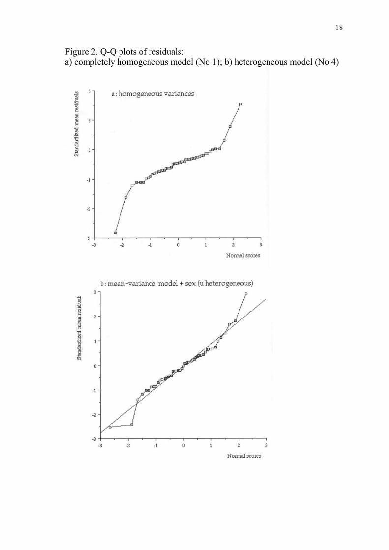
Diagnostic tools such as Quantile-Quantile plots of residuals also clearly

showed that heteroskedastic models fit better the data than homoskedastic

ones (figure 2ab).

4. DISCUSSION

The approach described in this paper represents a further step in analyzing

heterogeneous variances within the framework of linear mixed models.

Including a data variance proportional to a power of the data expectation

had been envisioned by several authors: see e.g., textbooks by Judge et al

(1985) (chapter 11) and Seber and Wild (2003), chapter 2.8. Box and Hill

12

(1974) have shown the relationship existing between the coefficient of this

power and the parameter of a Box-Cox transformation for stabilizing

variance. The interest of our approach is to combine this modelling device

with others such as the structural approach based on exogenous explanatory

variables and heterogeneity of both residual and random effect components

of variance to make models more realistic. At this stage, models are

specified very simply to make them parsimonious. This is especially

important as far as dispersion parameters are concerned, since there is

generally less information in the data about them as there is for location

parameters. However, other mean-variance dependency functions can be

considered (Davidian and Carroll, 1987) as well as more complicated

relationships between random and residual components of variance. The

procedure described here is flexible enough to cope with all these

modelling variants.

Regarding inferential aspects, our choice was directed towards EM-REML

type procedures although other options could have been envisioned. In

particular, ML was discarded as it is known to be very sensitive regarding

fixed effects with respect to misspecification in the functional form of the

variance contrarily to GLS (Carroll and Ruppert, 1982a). Our approach has

close links with the structural inference analysis developed by Levenbach

(1973) and the iterative procedures developed by Box and Hill (1974),

Pritchard et al (1977) for purely fixed linear models and variance functions

involving only a mean-variance relationship. Connections also exist with

the different weighted least squares procedures investigated by Beal and

Sheiner (1988). All these methods rely on iterative GLS and some

approximation is made when integrating out fixed effects to get the

marginal or posterior density of dispersion parameters (Seber and Wild,

2003). Intensive stochastic procedures would be required to overcome this

difficulty.

13

This method might be also extended to take into account other distributions

than the normal, such as the lognormal and the gamma. This again will

imply implementation of MCMC algorithms (Robert and Casella, 1999;

Sorensen and Gianola, 2002). Finally, as results are known to be sensitive

to distribution assumptions and to outliers, robust procedures should be

examined along the lines of current works in this area (see e.g., Carroll and

Ruppert, 1982b).

14

References

Beal S.L., Sheiner L.B. (1988), Heteroscedastic nonlinear regression, Technometrics,

30, 327-338

Box G.E.P., Hill W.J. (1974), Correcting inhomogeneity of variance with power

transformation weighting, Technometrics, 16, 385-389.

Brotherstone S., Hill W.G. (1986), Heterogeneity of variance amongst herds for milk

production, Animal Production, 42, 297-303.

Carroll R.J., Ruppert D. (1982a), A comparison between maximum likelihood and

generalized least squares in a heteroscedastic model, Journal of the American

Statistical Association, 77, 878-882.

Carroll R.J., Ruppert D. (1982b), Robust estimation in heteroscedastic linear models,

The Annals of Statistics, 10, 429-441.

Davidian M., Carroll R.J. (1987), Variance function estimation, Journal of the

American Statistical Association, 82, 1079-1091.

Davidian M., Giltinian D.M. (1995), Nonlinear models for repeated measurement data,

Chapman & Hall, New-York.

Dempster A., Laird N., Rubin R. (1977), Maximum likelihood estimation from

incomplete data via the EM algorithm, Journal of the Royal Statistical Society B,

39,1-38.

Dempster A., Selwyn M.R., Patel C.M., Roth A.J. (1984) Statistical and computational

aspects of mixed model analysis, Applied Statistics, 33, 203-214.

Foulley J.L. (1997), ECM approaches to heteroskedastic mixed models with constant

variance ratios, Genetics Selection Evolution, 29, 297-318.

Foulley J.L. (2002), Algorithme EM: théorie at application au modèle mixte, Journal de

la Société Française de Statistique, 143, 57-109.

Foulley J.L., Gianola D., San Cristobal M., Im S. (1990), A method for assessing extent

and sources of heterogeneity of residual variances in mixed linear models, Journal

of Dairy Science, 73, 1612-1624.

Foulley J.L., San Cristobal M., Gianola D., Im S. (1992), Marginal likelihood and

Bayesian approaches to the analysis of heterogeneous residual variances in mixed

linear models, Computational Statistics and Data Analysis, 13, 291-305.

Foulley J.L., Quaas R.L. (1995), Heterogeneous variances in Gaussian linear mixed

models, Genetics Selection Evolution, 27, 211-228.

15

Foulley J.L., Quaas R.L., Thaon d’Arnoldi C. (1998), A link function approach to

heterogeneous variance components, Genetics Selection Evolution, 30, 27-43.

Garrick D.J., Pollak E.J., Quaas R.L., Van Vleck L.D. (1989), Variance heterogeneity in

direct and maternal weight traits by sex and percent purebred for Simmental sired

calves, Journal of Animal Science, 67, 2515-2528.

Lange K. (1995), A gradient algorithm locally equivalent to the EM algorithm. Journal

of the Royal Statistical Society B, 57, 425-437.

Leonard T. (1975), Bayesian approach to the linear model with unequal variance,

Technometrics, 17, 95-102.

Levenbach H. (1973), The estimation of heteroscedasticity from a marginal likelihood

function, Journal of the American Statistical Association, 68, 436-439.

Meng X.L., Rubin D.B. (1993), Maximum likelihood estimation via the ECM

algorithm: a general framework, Biometrika, 80, 267-278.

Pritchard D.J., Downie J. Bacon D.W. (1977), Further consideration of

heteroskedasticity in fitting kinetic models. Technometrics, 19, 109-115

Robert C.P., Casella G. (1999), Monte Carlo Statistical Methods, Springer, Berlin.

Robert-Granié C., Bonaiti B., Boichard D., Barbat A. (1999), Accounting for variance

heterogeneity in French dairy cattle genetic evaluation, Livestock Production

Science, 60, 343-357

Rosa G.J.M., Padovani C.R., Gianola D. (2003), Robust linear mixed models with

normal/independent distributions and Bayesian MCMC implementation,

Biometrical Journal, 45, 573-590.

San Cristobal M., Foulley J.L., Manfredi E. (1993), Inference about multiplicative

heteroskedastic components of variance in a mixed linear Gaussian model with an

application to beef cattle, Genetics, Selection, Evolution, 25, 3-30

San Cristobal M., Elsen J.M., Bodin L., Chevalet C. (2001), Prediction of the response

to a selection for canalisation of a continuous trait in animal breeding, Genetics

Selection Evolution, 33, 249-271

San Cristobal M., Robert-Granié C., Foulley J.L. (2002), Hétéroscédasticité et modèles

linéaires mixtes: théorie et applications en génétique quantitative, Journal de la

Société Française de Statistique, 143, 155-165.

Seber G.A.F., Wild C.J. (2003), Nonlinear regression, Wiley and Sons, New-York

Sorensen D., Gianola D. (2002), Likelihood, Bayesian, and MCMC Methods in

Quantitative Genetics, Springer Verlag.

16

Visscher P.M., Thompson R., Hill W.G. (1991), Estimation of genetic and

environmental variances for fat yield in individual herds and an investigation into

heterogeneity of variance between herds. Livestock Production Science, 28, 273-

290

Weigel K.A., Gianola D., Yandel B.S., Keown J.F. (1993) Identification of factors

causing heterogeneous within herd variance components using a structural model

for variances. Journal of Dairy Science, 76, 1466-1478

17

Figure 1. Mean variance relationship

18

Figure 2. Q-Q plots of residuals: a) completely homogeneous model (No 1); b) heterogeneous model (No 4)

19

Table I: Likelihood statistics for testing dispersion parameters in heteroskedastic mixed models: choice of a structural model for residual variances

Model Likelihood Test

No Location Residual Dam par -2L -2BIC H0 Comp df Statistic P-value

(1) µ+T+S+L µ∗+T*+S*+L* µ’: σu cst 7 3232.0704 3272.3828

(2) µ+T+S+L µ∗+S*+L* µ’: σu cst 5 3259.2976 3288.0921 T*=0 2-1 2 27.2272 10E-6

(3) µ+T+S+L µ∗+T*+L* µ’: σu cst 6 3233.9926 3268.5460 S*=0 3-1 1 1.9222 0.1656

(4) µ+T+S+L µ∗+T*+S* µ’: σu cst 5 3271.3391 3300.1336 L*=0 4-1 2 39.2687 3E-9

a: Covariates: µ: intercept; T: treatment; S:sex ; L: litter size Covariates for log parameters coded as: (eg for Treatment T), location (T), residual variance (T*), T-component (T’) b: par: number of dispersion parameters: ; L=maximum of the loglikelihood (REML version) c: Likelihood ratio (LR) test based on difference in -2L between the full and reduced models;

20

Table II: Likelihood statistics for testing dispersion parameters in heteroskedastic mixed models: choice of a model for the u or ratio components

Model Likelihood Test

No Location Residual Dam par -2L -2BIC H0 Comp df Statistic P-value

(1) µ+T+S+L µ∗+T*+L* µ’+T’+L’, or

µ’’+T’’+L’’

10 3230.86 3288.45

(2) µ+T+S+L µ∗+T*+L* 0 1ln lni iu eb bσ σ= +

7 3232.36 3272.67 Model 2 2-1 3 1.5046 0.6812

(3) µ+T+S+L µ∗+T*+L* µ’’: ratio cst

6 3239.31 3273.86 T’’=L’’=0

1 1b =

3-1

3-2

4

1

8.4495

6.9448

0.0764

0.0084

(4) µ+T+S+L µ∗+T*+L* µ’: σu cst

6 3233.99 3268.55 T’=L’=0

1 0b =

4-1

4-2

4

1

3.1362

1.6315

0.5353

0.2015

a: Covariates: µ: intercept; T: treatment; S:sex ; L: litter size Covariates for log parameters coded as: (eg for Treatment T), location (T), residual variance (T*), T-component (T’), and u to residual variance log-ratio (T’’) b: par: number of dispersion parameters: L=maximum of the loglikelihood (REML version) c: Likelihood ratio (LR) test based on difference in -2L between the full and reduced models;

21

Table III: Likelihood statistics for testing dispersion parameters in heteroskedastic mixed models: choice of a model for residual variances including a mean-variance relationship

Modela Likelihoodb Testc

No Location Residual Dam par -2L -2BIC H0 Comp df Statistic P-value

(1) µ+T+S+L µ∗ µ’: σu cst 2 3316.68 3328.20

(2) µ+T+S+L µα, µ∗ µ’: σu cst 3 3259.16 3276.44 α=0 2-1 1 57.51 1E-14

(3) µ+T+S+L µα, µ∗+S* µ’: σu cst 4 3241.88 3264.92 S*=0 3-2 1 17.28 3E-5

(4) µ+T+S+L µα, µ∗+S* ( )0 1,b b 5 3231.26 3260.06 1 0b = 4-3 1 10.62 0.001

a: Covariates: µ: intercept; T: treatment; S:sex ; L: litter size Covariates for log parameters coded as: (eg for Treatment T), location (T), residual variance (T*), T-component (T’) b: par: number of dispersion parameters: ; L=maximum of the loglikelihood (REML version) ; -2BIC=-2L+par log(N-#fixed effects) c: Likelihood ratio (LR) test based on difference in -2L between the full and reduced models;

22

Table IV : Estimation of parameters in different models for birth weight of pup rats

Parameter (1) (2) (3) (4)

Intercept 640.28±11.19 643.21±12.35 644.76±10.16 650.29±8.80

Treatment -42.85±15.04 -44.77±15.85 -48.44±15.23 -59.56±13.70

-85.87±18.18 -90.30±19.85 -82.49±18.45 -92.23±17.18

Sex 35.91±4.75 34.18±3.91 34.03±3.89 33.05±4.68

Litter size -12.90±1.88 -13.19±2.20 -13.20±2.01 -13.56±2.17

-2BIC 3328.28 3268.55 3272.67 3260.06 Intercept : control, female, litter size equal to 12 Treatement : 1st row : Low dose-Control ; 2nd row: High dose-Control Sex : male-female ; Litter size : coefficient of regression (1) Homogeneous ; (2) Residual=mu+treatment+litter size

(3) Residual=idem ; 1/i i

bu e cstσ σ = ; (4) Residual=muα, sex ; 1/

i i

bu e cstσ σ =