1 On Pairwise Granger causality Modelling and Econometric Analysis of Selected Economic Indicators Olushina Olawale Awe Department of Mathematics, Obafemi Awolowo University, Ile-Ife, Nigeria E-mail :[email protected]+2348034558906 Abstract. The goal of most empirical studies in econometrics and other social sciences is to determine whether a change in one variable causes a change in or helps to predict another variable. Granger causality modeling approach is quite popular in experimental and non- experimental fields which involve some dynamic econometric time series methodologies. In this paper, Granger causality and co-integration tests were employed in the empirical modelling of seven economic indicators in Nigeria. The results alternated between bi- directional, uni-directional and no causality among the economic indicators considered. Prior to the Granger causality tests, we tested for stationarity in the variables using the Augmented Dickey-Fuller (ADF) procedure. The variables proved to be integrated of either I(1) or I(2). Johansen co-integration test reveals that at 5% level of significance, we have at least four co-integrating pairs among the variables. This verifies the fact that when two or more time series are co-integrated, there must be either bi-directional or uni- directional Granger causality between them. Our findings reveal that Government Investment, Real Money Supply and Government Expenditure Granger causes output growth in Nigeria. We finally relate these results with popular postulations in economic theory. Key Words: Causality, GDP, Co-integration, Prediction, Economic theory. 1.0 Introduction. Causality can be described as the relationship between cause and effect. Basically, the term ‘causality’ suggests a cause and effect relationship between two sets of variables, say, Y and X . Recent advances in graphical models and the logic of causation have given rise to new ways in which scientists analyze cause-effect relationships (Pearl, 2012). Runes (1962) highlighted nine basic definitions of causality which was also captured by Hinkelmann and Kempthorne (2008) as follows:
Transcript
1
On Pairwise Granger causality Modelling and Econometric Analysis of Selected Economic Indicators
Olushina Olawale Awe
Department of Mathematics, Obafemi Awolowo University, Ile-Ife, Nigeria
The goal of most empirical studies in econometrics and other social sciences is to determine whether a change in one variable causes a change in or helps to predict another variable. Granger causality modeling approach is quite popular in experimental and non-experimental fields which involve some dynamic econometric time series methodologies. In this paper, Granger causality and co-integration tests were employed in the empirical modelling of seven economic indicators in Nigeria. The results alternated between bi-directional, uni-directional and no causality among the economic indicators considered.
Prior to the Granger causality tests, we tested for stationarity in the variables using the Augmented Dickey-Fuller (ADF) procedure. The variables proved to be integrated of either I(1) or I(2). Johansen co-integration test reveals that at 5% level of significance, we have at least four co-integrating pairs among the variables. This verifies the fact that when two or more time series are co-integrated, there must be either bi-directional or uni-directional Granger causality between them.
Our findings reveal that Government Investment, Real Money Supply and Government Expenditure Granger causes output growth in Nigeria. We finally relate these results with popular postulations in economic theory.
Causality can be described as the relationship between cause and effect. Basically, the term ‘causality’ suggests a cause and effect relationship between two sets of variables, say, Y and X. Recent advances in graphical models and the logic of causation have given rise to new ways in which scientists analyze cause-effect relationships (Pearl, 2012).
Runes (1962) highlighted nine basic definitions of causality which was also captured by Hinkelmann and Kempthorne (2008) as follows:
2
(1)A relation between events, process or entities in the same time series subject to several conditions.
(2)A relationship between events, processes or entities in a time series such that when one occurs, the other follows invariably.
(3)A relationship among variables such that one has the efficacy to produce or alter another.
(4)A relationship among variables such that without one, the other could not occur.
(5)A relationship between experienced events, processes or entities and extra-experimential events, processes or entities.
(6)A relation between something and itself (self-causality).
(7)A relation between an event, process or entity and the reason or explanation for it.
(8)A relation between an idea and an experience and
(9)A principle or category incorporating into experience one of the previous ones.
However, in recent times, Granger causality modelling has received considerable attention and use in many areas of research. Since the concept of Granger (non) causality was introduced by Granger (1969), it has become a popular concept in econometrics and many other fields of human endeavour.
In line with most of the literatures in econometrics, one variable is said to Granger cause the other if it helps to make a more accurate prediction of the other variable than had we only used the past of the latter as predictor. Granger causality between two variables cannot be interpreted as a real causal relationship but merely shows that one variable can help to predict the other one better.
Given two time series variables Xt and Yt, Xt is said to Granger cause Yt if Yt can be better predicted using the histories of both Xt and Yt than it can by using the history of Yt alone. In this paper, we model selected economic indicators using Pairwise Granger causality analysis as proposed by Granger (1969).The rest of the paper is structured as follows: Section two discusses the literature review, section three is on the data and methodology used in the study, section four is on the empirical analysis and results while section five discusses the results and concludes the paper.
3
2.0 Literature Review.
Many researchers in the field of Time Series Econometrics have used Granger causality procedure to study the causal interactions that exists among economic indicators in various countries of the world. Moreover, several intelligent articles have surfaced in literature on the use of Granger causality tests to analyze time series data since its introduction by Granger(1969).
Some of the articles include: Granger CWJ(1969), Granger CWJ(1980), Granger CWJ( 1988), Swanson and Granger(1997), Entner et al (2010), Mohammed et al(2010), Chu and Chymour (2008), Arnold et al (2007), Eichler and Didelez(2009), Clarke and Mirza (2006), Erdal et al (2008), Pearl(2012) just to mention a few. Others include: Shojaie and Michailidis (2010), Moneta et al (2011),Chen and Hsiao (2010),White et al(2011), Zou et al (2010), Havackova-Schindler et al (2007), Haufe et al (2010), Eichler and Didelez (2007),Cheng(1996),Cheng et al(1997),Toda et al (1994) etc.
Although, flurries of articles have been written on the topic, regrettably, the comparison is usually done among smaller groups of variables. This study tends to contribute to the theoretical and empirical literature on the topic and examines the Pairwise Granger causality analysis of selected economic indicators in Nigeria. We also offer some theoretical economic underpinnings of the related variables involved in the study.
3.0 Data and Methodology.
We used secondary data obtained from the Central Bank of Nigeria Statistical Bulletin in this study.
Data on seven economic indicators were obtained for a period of 35years (1970-2004). The Economic variables considered are: Gross Domestic Product, Money Supply, Investment, Exchange Rate, Inflation Rate, Government Expenditure, and Interest Rate on Lending.
Data on these variables collected over a period of 35 years were subjected to econometric analysis to determine Granger causality by use of bi-variate Vector Autoregressive (VAR) Models. Traditionally, most economic variables are non-stationary; hence unit root tests were performed on all the variables. All the variables were found to be non-stationary and integrated of either I(1) or I(2).
Johansen’s co-integration test reveals that at 5% level of significance there is at least four co-integrating equations in the study.
4
Vector auto-regressive modelling approach was used to model the variables.
We determine the best lag length by the use of Akaike Information Criteria (AIC) and Schwartz Information Criteria(SIC).Therefore, we used a lag length of 2 in the study.
Prior to the Pairwise Granger causality tests, we first conduct unit root tests to determine if the variables are stationary and to detect their order of integration.
Granger and Newbold (1974) noted that the regression results from the VAR models with non-stationary variables will be spurious.
We use Johansen and Juselius (1990) test to check for the presence of co-integration among the series. Two time series are co-integrated if there is a long run relationship between them. We then capture the interrelationships among the variables with Pairwise Granger causality tests.
3.1 Steps involved in testing for Granger causality (Gujarati, 1995).
The steps involved in testing for the direction of causality between two economic series say, and are as follows:
1. Regress current on all past values and other variables, but do not include the lagged variables in this regression. Hence, from this regression, obtain the residual sum of squares.
2. Now run the regression including the lagged variable(unrestricted regression).From this regression, obtain the unrestricted residual sum of squares( )
3. Test the null hypothesis Ho: i.e. lagged terms do not belong in the regression. 4. To test this hypothesis, we apply the F-test given by;
F = ⁄
⁄ ……………….. (3)
This follows the F-distribution with M and N-K degrees of freedom. M is the number of lagged terms and K is the number of parameters of parameters estimated in the restricted regression.
5 If the F-value exceeds the critical F-values at the chosen level of significance, or if the P-value is less than the alpha level of significance, we reject the null hypothesis in which case the lagged values belong in the regression. This is another way of saying that Granger causes . Gujarati (1995)
6 Step 1-5 can be repeated to test model (2) i.e. to test whether Granger causes Xt.
This methodology is highly sensitive to lag length selection when conducting a Granger causality analysis.
5
4.0 Empirical Analyses and Results.
This section contains the various fundamental results of analysis from this research.
4.1 Unit root tests.
Traditionally, most economic variables are non-stationary; hence we test for the presence of unit-roots using the Augmented Dickey-Fuller tests.
Dickey(1976) and Fuller (1976) noted that the least squares estimator of the VAR model in the Granger causality analysis is biased in the presence of unit root and this bias can be expected to reduce the accuracy of forecasts.
Given an AR (p) process:
∑ Є (1)
Є 0,
which can be written through recursive replacement with differenced terms, as
∆ ∑ ∆ (2)
Є 0, Where = , ∑ 1, 1, …… ,
The ADF tests the null hypothesis that p= 0 against the alternative p
<0. If the AR (p)
process has a unit root, and p =0. If the process is stationary, then p
<0.
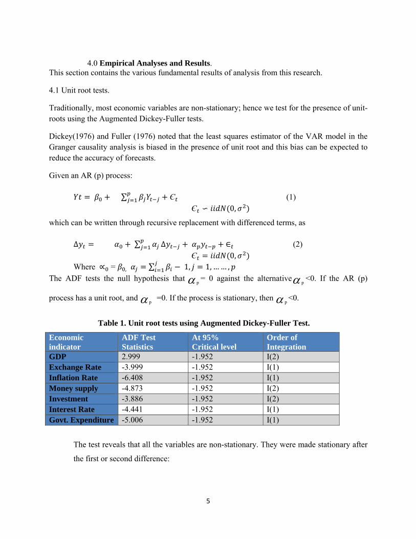
Table 1. Unit root tests using Augmented Dickey-Fuller Test.
The test reveals that all the variables are non-stationary. They were made stationary after
the first or second difference:
6
GDP became stationary after the second difference, Exchange Rate became stationary after the
first difference, Inflation Rate became stationary after the first difference, Money supply became
stationary after the second difference, Investment became stationary after the second difference,
Interest rate became stationary after the first difference and Government Expenditure became
stationary after the first difference. Granger and Newbold (1974) noted that the regression results
from the VAR models of the Granger causality tests using non-stationary variables will be
spurious. To avoid this, we will run the regression with the stationary variables after
differencing.
4.2 Co-integration Tests
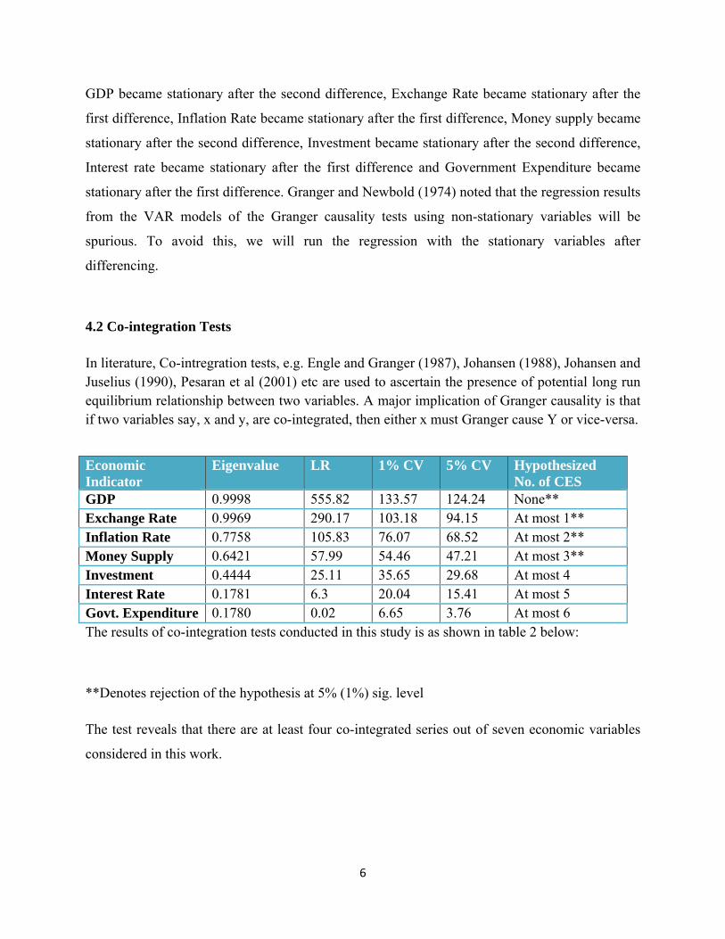
In literature, Co-intregration tests, e.g. Engle and Granger (1987), Johansen (1988), Johansen and Juselius (1990), Pesaran et al (2001) etc are used to ascertain the presence of potential long run equilibrium relationship between two variables. A major implication of Granger causality is that if two variables say, x and y, are co-integrated, then either x must Granger cause Y or vice-versa.
The results of co-integration tests conducted in this study is as shown in table 2 below:
**Denotes rejection of the hypothesis at 5% (1%) sig. level
The test reveals that there are at least four co-integrated series out of seven economic variables
considered in this work.
Economic Indicator
Eigenvalue LR 1% CV 5% CV Hypothesized No. of CES
GDP 0.9998 555.82 133.57 124.24 None** Exchange Rate 0.9969 290.17 103.18 94.15 At most 1** Inflation Rate 0.7758 105.83 76.07 68.52 At most 2** Money Supply 0.6421 57.99 54.46 47.21 At most 3** Investment 0.4444 25.11 35.65 29.68 At most 4 Interest Rate 0.1781 6.3 20.04 15.41 At most 5 Govt. Expenditure 0.1780 0.02 6.65 3.76 At most 6
7
4.3 Pairwise Granger causality Tests
We test for the absence of Granger causality by estimating the following VAR model:
)2......(......
)1......(......
11110
11110
tptptptptt
tptptptptt
VYdYdXcXccX
UXbXbYaYaaY
Testing
01
210
:
0...:
NotHH
against
bbbH p
is a test that Xt does not Granger-cause Yt.
Similarly, testing H0: d1= d2=…= dp=0 against
H1: Not H0 is a test that Yt does not Granger cause Xt.
In each case, a rejection of the null hypothesis implies there is Granger causality between the variables.
In testing for Granger causality, two variables are usually analyzed together, while testing for their interaction. All the possible results of the analyses are four:
Unidirectional Granger causality from variable Yt to variable Xt.
Unidirectional Granger causality from variable Xt to Yt
Bi-directional causality and
No causality
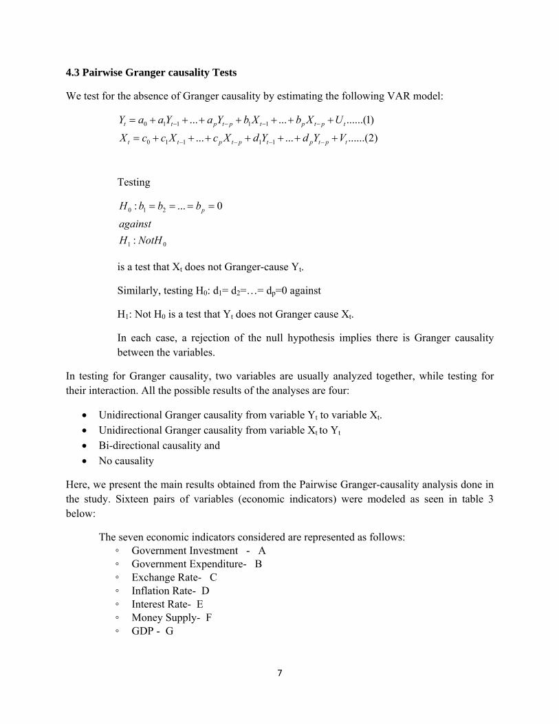
Here, we present the main results obtained from the Pairwise Granger-causality analysis done in the study. Sixteen pairs of variables (economic indicators) were modeled as seen in table 3 below:
The seven economic indicators considered are represented as follows: ◦ Government Investment - A ◦ Government Expenditure- B ◦ Exchange Rate- C ◦ Inflation Rate- D ◦ Interest Rate- E ◦ Money Supply- F ◦ GDP - G
8
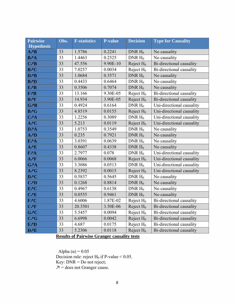
Results of Pairwise Granger causality tests
Alpha (α) = 0.05 Decision rule: reject H0 if P-value < 0.05. Key: DNR = Do not reject; ↗ = does not Granger cause.
Pairwise Hypothesis
Obs. F-statistics P-value Decision Type for Causality
A B 33 1.5786 0.2241 DNR H0 No causality B A 33 1.4463 0.2525 DNR H0 No causality C B 33 47.556 9.90E-10 Reject H0 Bi-directional causality B C 33 7.0257 0.0034 Reject H0 Bi-directional causality D B 33 1.0684 0.3571 DNR H0 No causality B D 33 0.4433 0.6464 DNR H0 No causality E B 33 0.3506 0.7074 DNR H0 No causality F B 33 13.166 9.30E-05 Reject H0 Bi-directional causality B F 33 14.934 3.90E-05 Reject H0 Bi-directional causality G B 33 0.4924 0.6164 DNR H0 Uni-directional causality B G 33 4.8519 0.0155 Reject H0 Uni-directional causality C A 33 1.2256 0.3089 DNR H0 Uni-directional causality A C 33 5.213 0.0119 Reject H0 Uni-directional causality D A 33 1.0753 0.3549 DNR H0 No causality A D 33 0.235 0.7921 DNR H0 No causality E A 33 3.0391 0.0639 DNR H0 No causality A E 33 0.8607 0.4338 DNR H0 No causality F A 33 2.7977 0.078 DNR H0 Uni-directional causality A F 33 6.0066 0.0068 Reject H0 Uni-directional causality G A 33 3.3086 0.0513 DNR H0 Uni-directional causality A G 33 8.2392 0.0015 Reject H0 Uni-directional causality D C 33 0.5837 0.5645 DNR H0 No causality C D 33 0.1268 0.8814 DNR H0 No causality E C 33 0.4967 0.6138 DNR H0 No causality C E 33 0.0555 0.9461 DNR H0 No causality F C 33 4.6006 1.87E-02 Reject H0 Bi-directional causality C F 33 20.3501 3.50E-06 Reject H0 Bi-directional causality G C 33 5.5457 0.0094 Reject H0 Bi-directional causality C G 33 6.6998 0.0042 Reject H0 Bi-directional causality E D 33 4.687 0.0175 Reject H0 Bi-directional causality D E 33 5.2306 0.0118 Reject H0 Bi-directional causality
9
5.0 Discussion and Conclusion.
The goal of this paper was to examine the interrelationships among certain economic indicators in Nigeria by using the concept of Granger causality tests developed by Granger(1969).
We used sixteen VAR models to test for Pairwise Granger (non) causality among the economic indicators and the following results were obtained:
No causality exists between Government Investment and Government Expenditure. Bi-directional causality exists between Exchange Rate and Government Expenditure, No causality exists between Inflation Rate and Government Expenditure, No causality exists between Interest Rate and Government Expenditure, Bi-directional causality exists between money supply and Government Expenditure, Uni-directional causality exists between GDP and Government Expenditure, Uni-directional causality exists between Exchange Rate and Government Expenditure, No causality exists between Inflation Rate and Government Investment, No causality exists between Interest rate and Government Investment in the ninth model, Uni-directional causality exists between money supply and Government Investment in the tenth model, Uni-directional causality exists between GDP and Government Investment in the eleventh model, No causality exists between Inflation Rate and Exchange Rate. No causality exists between Interest Rate and Exchange Rate, Bi-directional causality exists between money supply and exchange rate in the fourteenth model,Bi-directional causality exists between GDP and Exchange rate, Bi-directional causality exists also between Interest Rate and Inflation Rate in the last VAR model.
More specifically, we can see that the following uni-directional and bi-directional causality exists between some selected economic indicators: Investment Granger causes GDP,Investment Granger causes Money Supply, Investment Granger causes Exchange Rate, Government Expenditure Granger causes GDP, The bi-directional causality results are: Exchange Rate Granger causes Government Expenditure, Government Expenditure Granger Causes Exchange Rate. Money Supply Granger causes Government Expenditure, Government Expenditure Granger causes Money Supply. Money Supply Granger cause Exchange Rate, Exchange Rate Granger cause Money Supply. GDP Granger causes Exchange Rate, Exchange Rate Granger causes GDP. Interest Rate Granger cause Inflation Rate, Inflation Rate Granger cause Interest Rate. The results here confirms the earlier co-integration tests that depicts we have at least four
cointegrated equations in the study.
However, as expected, given the Granger causality test results, few linkages between the series can be established in line with economic theory and postulations.
10
5.1 Discussion on the Pairwise economic analysis of the economic indicators.
The bi-directional and uni-directional Pairwise Granger causality analysis results in this study are hereby discussed in relation with some economic theory and postulations.
5.1.1 Investment and GDP The effect of investment on GDP is positive, as increase in capital investment results in higher levels of output, as aggregate demand increases. Furthermore, it is important to note that, rise in investment results in economic boom and growth.
Also, GDP can also be an independent variable or determinant of investment- relatively high increase in the GDP of an economy, constitutes an attractive place for capital investment, notably, Foreign Direct Investments (FDIs).
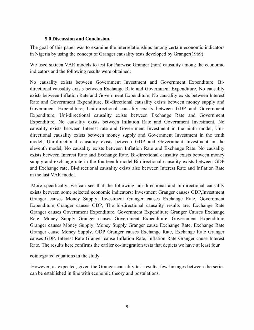
5.1.2 Money Supply and Investment
This could be illustrated with the use of the Mundell-fleming Economic Model- IS/LM model.
Where IS = Goods market and LM= Money Market.
Figure 1:Showing graphical illustration of the economy using theMundell-Fleming Model
As illustrated in figure 1 above- Expansionary monetary policy, which implies an increase in the money supply, hence LM shifts to the right causing interest rates to fall from i0 to i1, because of the excess supply at point A the economy moves to point B.
As a result of the declining interest rate, Investment projects become very attractive, because the opportunity cost of investing is lower than the subsequent return on investments.
11
Increase in investment, causes aggregate demand to increase hence output also increases relatively. (M. Gartner p.83, 84).
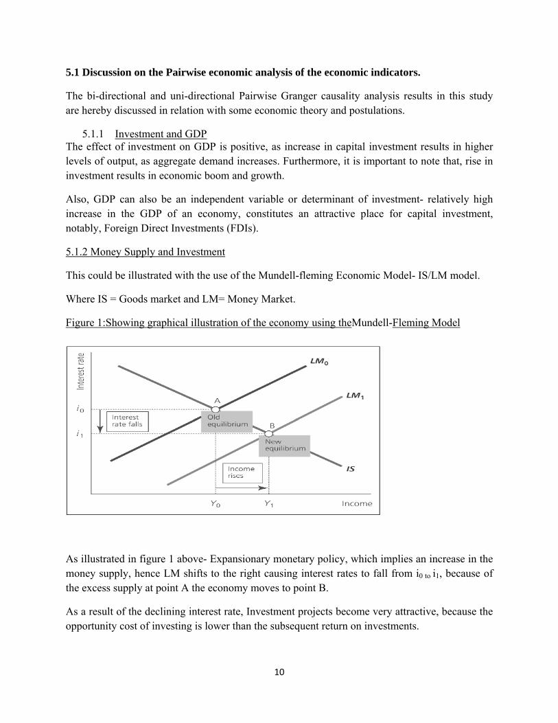
5.1.3 Investment and Exchange Rate
Figure 2: Illustration of the economy using the IS/LM/FE model
Adapted from: Macroeconomics 3rd edition by M. Gartner
As illustrated in figure 2 above, with the assumption that exchange rates in the economy is flexible (as monetary policy is only effective under flexible exchange rates), expansionary monetary policy will result in the interest falling below the interest rate of the world (i’< iw) causing capital investment outflows i.e. Investors will seek better returns in other countries, and this results in an increase in the real exchange rate (depreciation). The opposite occurs with contractionary monetary policy [Ceteris paribus].
12
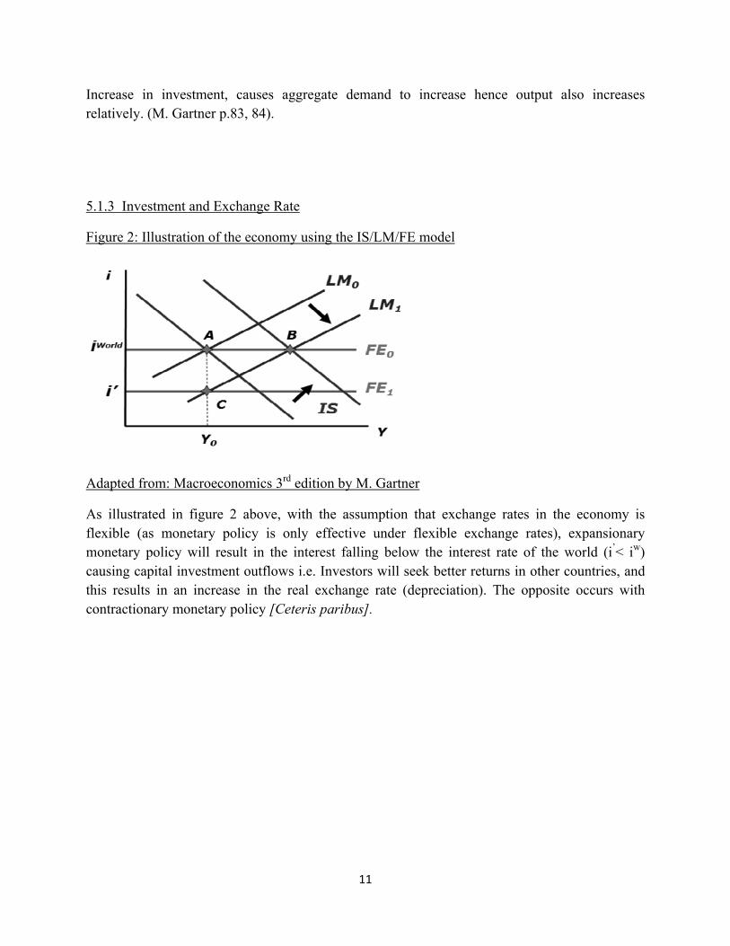
5.1.4 Government Expenditure and Exchange Rate
Figure 3: Showing the impact of fiscal policy on the economy
Adapted from: Macroeconomics 3rd edition by M. Gartner
As shown graphically above, expansionary fiscal policy i.e. increase in government expenditure under fixed exchange rate (it is only effective under this condition), will shift IS to the right immediately. Depending on the adjustment dynamics of the other markets (LM and FE), even though IS as shifted to point C, the other markets could still be at point A as they will only react in the long run. This creates excess demand in the goods market, causing interest rate to increase above the interest rate of the world (i’ >iw), leading to currency appreciation (fall in Real exchange rate) on the short-run.
However, on the long-run, because the economy operates on a fixed exchange rate, the Central Bank will have to increase the money supply, to accommodate the excess demand, therefore LM shifts to the right and a new equilibrium is reached at point B.
Therefore the effect of Government expenditure on GDP is positive-as the economy moves to point B and output increases (GDP ). [M. Gartner, p. 83-65].
13
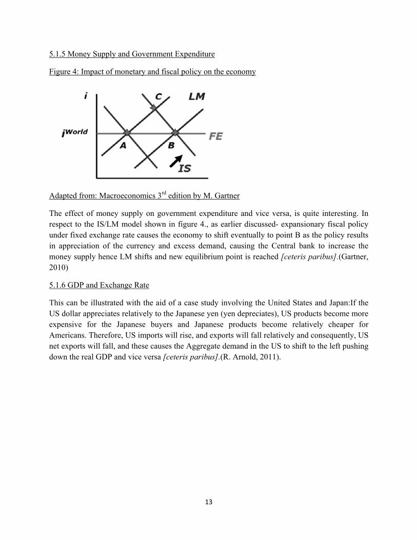
5.1.5 Money Supply and Government Expenditure
Figure 4: Impact of monetary and fiscal policy on the economy
Adapted from: Macroeconomics 3rd edition by M. Gartner
The effect of money supply on government expenditure and vice versa, is quite interesting. In respect to the IS/LM model shown in figure 4., as earlier discussed- expansionary fiscal policy under fixed exchange rate causes the economy to shift eventually to point B as the policy results in appreciation of the currency and excess demand, causing the Central bank to increase the money supply hence LM shifts and new equilibrium point is reached [ceteris paribus].(Gartner, 2010)
5.1.6 GDP and Exchange Rate
This can be illustrated with the aid of a case study involving the United States and Japan:If the US dollar appreciates relatively to the Japanese yen (yen depreciates), US products become more expensive for the Japanese buyers and Japanese products become relatively cheaper for Americans. Therefore, US imports will rise, and exports will fall relatively and consequently, US net exports will fall, and these causes the Aggregate demand in the US to shift to the left pushing down the real GDP and vice versa [ceteris paribus].(R. Arnold, 2011).
14
5.1.7 Money Supply and Exchange Rate
Figure 5: Showing the IS/LM/FE model
Adapted from: Macroeconomics 3rd edition by M. Gartner
In reference to the Mundell-fleming Model (IS/LM/FE), this analysis is similar to that which explained earlier between investments and exchange rate as these variables constitute virtually the same effects.
As illustrated in figure 5 above, with the assumption that exchange rates in the economy is flexible (as monetary policy is only effective under flexible exchange rates), expansionary monetary policy i.e. increase in money supply, will result in the interest falling below the interest rate of the world (i’< iw) causing capital investment outflows i.e. Investors will seek better returns in other countries, and this results in excess supply of the country’s currency, leading to an increase in the real exchange rate (depreciation). The opposite occurs with contractionary monetary policy i.e. reduction in the money supply results in a decrease in the real exchange rate (appreciation)[Ceteris paribus].(M. Gartner, 2009).
5.1.8 Interest Rates and Inflation
Theoretically, there is a negative relationship between interest rate and Inflation. This is based on the assumption that humans are rational (homo economicus). It is believed that as interest rates increases, the incentive to save increases and saving becomes more attractive, this results in less spending and consequently inflation falls and vice versa [ceteris paribus].
However in reality, we often notice the opposite- despite increase in interest rates, people tend to spend even more and this could be explained in terms of individuals having expectations of inflation whether adaptive or rational, leading to increase in consumer spending.
15
Furthermore, high levels of inflation could force the central bank of the respective country to increase interest rates which is expected to pass on to individuals in terms of increase in interest on loans and savings offered by banks. Hence, reducing spending and deflating the economy (reducing inflation). [Bank of England, 2010].
In conclusion, all these economic indicators majorly influence the Nigerian Economy positively
in terms of growth and development and also negatively in terms of slumps, hyper-inflation,
recessions, unemployment and ultimately depressions. It is noteworthy however, that the finding
of causality between some of the variables here does not mean that movement in one variable
physically cause movements in another. Rather, causality simply implies chronological ordering
of movements in the time series.
Although as expected, in line with the Granger causality results above, few linkages between the
economic series has been established in line with economic theory and postulations. Therefore
the causal effects, either bi-directional or unidirectional are dependent on the various economic
policies, both fiscal and monetary, conducted by the economic policymakers in Nigeria.
However, the field of time series econometrics is evolving, some of the results and tests
presented here are in some cases tentative; therefore a lot more other multivariate modelling
methods shall be explored in our future research.
16
References
Arnold, A. (2011) Macroeconomics. 10th ed. USA: Cengage Learning. Arnold, A., Liu, Y., & Abe, N. (2007).Temporal Causal Modeling with Graphical Granger Methods.KDD’07 Proceedings of the 13th ACM SIGKDD International Conference Knowledge Discovery and Data Mining. New York, NY: ACM .
Bank of England (2011): How do Interest Rates Affect Inflation (Internet)Available on :http://www.bankofengland.co.uk/education/Pages/targettwopointzero/inflation/ratesaffectinflation.aspx? Chu, T.&Glymlour, C. (2008). Search for Additive Nonlinear Time Series Causal Models.Journal of Machine Learning Research. 9,967-991.
Clarke, J.A and Mirza S.(2006). A Comparison of Some Common Methods for Detecting Granger Non-Causality. Journal of Statistical Computation and Simulation, 76, 207-231.
Entner D., & Hoyer, P.O. (2010).On Causal Discovery from Time Series Data Using FCI.Proceedings on the 5th European Workshop on Probabilistic Graphical Models (PGM). Helsinki, Finland.
Erdal, G., H. Erdal and K. Esengun (2008). The causality between Energy Consumption and Economic Growth in Turkey. Energy Policy, 36:3838-3842.
Gartner, M. (2010) Macroeconomics. 3rd ed. USA: Pearson Education.P. 83-88. Granger, C.W.J. (1969). Investigating Causal Relations by Econometric Models and Cross Spectral Methods.Econometrica.37:424-35.
Granger, C.W.J. (1980).Testing for causality.A Personal Viewpoint. Journal of Economic Dynamic and Control, 2(4), 329-352.
Granger, C.W.J. (1988). Some Recent Developments in a concept of Causality. Journal of Econometrics, 39(1),199-211.
Haufe, S., Muller, K-R., Nolte, G., & Kramer, N. (2010).Sparse Causal Discovery in Multivariate Time Series. JMLR Workshop and Conference Proceedings, 6, 97-106. NIPS 2008 workshop on causality.
Hlavackova-Schlinder, k., Palvus, M., Vejmelka, M.& Bhattacharya, J. (2007). Causality detection based on information-theoretic approaches in time series analysis. Physics Reports, 441, 1-46.
17
Mohammed, Y. ,& Nishida T. (2010). Mining Causal Relationships in Multidimensional Time Series. Studies on Computational Intelligence, 260, 309-338.
Moneta, A. ,Chalb, N., Entner , D., & Hoyer, P. (2011). Causal Search in Structural Vector Autoregressive Models. JMLR : Workshops and Conference Proceedings. 12, 95-118.
Pearl, Judea(2012). Correlation and Causation-the Logic of Co-habitation. Written for the European Journal of Personlity, Special Issue.
Shajoaie, A., &Michailidis, G. (2010). Discovering Graphical Granger Causality using the truncating lasso penalty. Bionformatics, 26(18), i517-i523.
Swanson, N.R., & Granger C.W.J. (1997).Impulse Response Functions Based on a Causal Approach to Residual Orthogonalization in Vector Autoregressions. Journal of the American Statistical Association, 92, 357-367.
White, H., Chalak, K., & Lu, X. (2011). Linking Granger Causality and the pearl causal model with Settable Systems. Journal of Machine Learning Research Workshop and Conference Proceedings. 12, 1-29.
Zou,C., Ladrou, C., Guo, S., &Feng, J. (2010). Identifying interactions in the time and frequency domains in local and global networks – A Granger Causality Approach. BMC Bioinformatics. 11(33).