Portfolio Management STUDY SESSIONS ■ Study Session 3 Behavioral Finance ■ Study Session 4 Private Wealth Management ■ Study Session 5 Portfolio Management for Institutional Investors ■ Study Session 6 Capital Market Expectations in Portfolio Management ■ Study Session 7 Economic Concepts for Asset Valuation in Portfolio ■ Study Session 8 Asset Allocation ■ Study Session 9 Management of Passive and Active Fixed-Income Portfolios ■ Study Session 10 Portfolio Management of Global Bonds and Fixed-Income Derivatives ■ Study Session 11 Equity Portfolio Management ■ Study Session 12 Equity Portfolio Management ■ Study Session 13 Alternative Investments for Portfolio Management ■ Study Session 14 Risk Management ■ Study Session 15 Risk Management Application of Derivatives ■ Study Session 16 Execution of Portfolio Decisions; Monitoring and Rebalancing ■ Study Session 17 Performance Evaluation and Attribution ■ Study Session 18 Global Investment Performance Standards is volume includes Study Sessions 9-12. COPYRIGHTED MATERIAL
Transcript
Portfolio Management
STUDY SESSIONS
■ Study Session 3 Behavioral Finance ■ Study Session 4 Private Wealth Management ■ Study Session 5 Portfolio Management for Institutional Investors ■ Study Session 6 Capital Market Expectations in Portfolio Management ■ Study Session 7 Economic Concepts for Asset Valuation in Portfolio ■ Study Session 8 Asset Allocation ■ Study Session 9 Management of Passive and Active Fixed-Income
Portfolios ■ Study Session 10 Portfolio Management of Global Bonds and Fixed-Income
Derivatives ■ Study Session 11 Equity Portfolio Management ■ Study Session 12 Equity Portfolio Management ■ Study Session 13 Alternative Investments for Portfolio Management ■ Study Session 14 Risk Management ■ Study Session 15 Risk Management Application of Derivatives ■ Study Session 16 Execution of Portfolio Decisions; Monitoring and
Rebalancing ■ Study Session 17 Performance Evaluation and Attribution ■ Study Session 18 Global Investment Performance Standards
The fixed-income market is one of the largest and fastest-growing segments of the global financial marketplace. Government and private debt currently constitute close to half of the wealth in international financial markets.
The basic features of the investment management process are the same for a fixed-income portfolio as for any other type of portfolio. Risk, return, and investment constraints are considered first. As part of this first step, however, an appropriate benchmark must also be selected based on the needs of the investor. For investors taking an asset-only approach, the benchmark is typically a bond market index, with success measured by the portfolio’s relative investment return. For investors with a liability-based approach, success is measured in terms of the portfolio’s ability to meet a set of investor-specific liabilities. The first reading addresses these primary elements of managing fixed-income portfolios and introduces specific portfolio management strategies. The second reading introduces additional relative-value methodologies.
READING ASSIGNMENTS
Reading 23 Fixed-Income Portfolio Management—Part I, Chapter 6, Sections 1-4Managing Investment Portfolios: A Dynamic Process, Third Edition, John L. Maginn, CFA, Donald L. Tuttle, CFA, Jerald E. Pinto, CFA, and Dennis W. McLeavey, CFA, editors
Reading 24 Relative-Value Methodologies for Global Credit Bond Portfolio ManagementFixed Income Readings for the Chartered Financial Analyst® Program, Second Edition, Frank J. Fabozzi, CFA, editor
S T U D Y S E S S I O N
9Management of Passive and
Active Fixed-Income Portfolios
P O R T F O L I O M A N A G E M E N T
ch01.indd 3 11/05/12 8:01 PM
ch01.indd 4 11/05/12 8:01 PM
R E A D I N G
23Fixed-Income Portfolio Management—Part I
by H. Gifford Fong and Larry D. Guin, CFA
LEARNING OUTCOMES Mastery The candidate should be able to:
a compare, with respect to investment objectives, the use of liabilities as a benchmark and the use of a bond index as a benchmark;
b compare pure bond indexing, enhanced indexing, and active investing with respect to the objectives, advantages, disadvantages, and management of each;
c discuss the criteria for selecting a benchmark bond index and justify the selection of a specific index when given a description of an investor’s risk aversion, income needs, and liabilities;
d describe and evaluate techniques, such as duration matching and the use of key rate durations, by which an enhanced indexer may seek to align the risk exposures of the portfolio with those of the benchmark bond index;
e contrast and demonstrate the use of total return analysis and scenario analysis to assess the risk and return characteristics of a proposed trade;
f formulate a bond immunization strategy to ensure funding of a predetermined liability and evaluate the strategy under various interest rate scenarios;
g demonstrate the process of rebalancing a portfolio to reestablish a desired dollar duration;
h explain the importance of spread duration; i discuss the extensions that have been made to classical immunization
theory, including the introduction of contingent immunization; j explain the risks associated with managing a portfolio against a
liability structure, including interest rate risk, contingent claim risk, and cap risk;
6 Reading 23 ■ Fixed-Income Portfolio Management—Part I
Mastery The candidate should be able to:
k compare immunization strategies for a single liability, multiple liabilities, and general cash flows;
l compare risk minimization with return maximization in immunized portfolios;
m demonstrate the use of cash flow matching to fund a fixed set of future liabilities and compare the advantages and disadvantages of cash flow matching to those of immunization strategies.
INTRODUCTION
Over the past 25 years, fixed-income portfolio management has moved from a sleepy backwater of the investment arena to the cutting edge of investment thought. Once, managers in the field concentrated on earning an acceptable yield to maturity and used a few relatively simple measures to control risk in the portfolio. Today, the port-folio manager has a stunning array of new tools at his disposal, capable of measuring and explaining the smallest variations in desired performance while simultaneously controlling risk with a variety of quantitative tools. This reading examines the results of that revolution in fixed-income portfolio management.
It is not our purpose to examine in great detail the analytical “tools of the trade”; these techniques are covered extensively elsewhere. Our focus is broader and empha-sizes the effective construction of a fixed-income portfolio and related risk issues. The fixed-income portfolio management process and the major themes in managing the fixed-income portion of a portfolio receive the emphasis in this reading.
The reading begins with a short review in Section 2 of the framework used for managing fixed-income portfolios. A fixed-income portfolio manager may manage funds against a bond market index or against the client’s liabilities. In the former approach, the chief concern is performance relative to the selected bond index; in the latter, it is performance in funding the payment of liabilities. Managing funds against a bond market index is covered in Section 3 while management against liabilities (asset/liability management or ALM) is covered in Section 4. The final section sum-marizes the reading.
A FRAMEWORK FOR FIXED-INCOME PORTFOLIO MANAGEMENT
To make our discussion easier to follow, let us revisit the four activities in the invest-ment management process:
1. setting the investment objectives (with related constraints);2. developing and implementing a portfolio strategy;3. monitoring the portfolio; and4. adjusting the portfolio.
These four steps as they apply to fixed-income portfolio management are shown in Exhibit 1. For ease of illustration, Exhibit 1 breaks the second activity (developing and implementing a portfolio strategy) into its individual parts and combines the third and fourth activities (monitoring and adjusting the portfolio).
1
2
ch01.indd 6 11/05/12 8:01 PM
A Framework for Fixed-Income Portfolio Management 7
Exh
ibit
1
The
Fixe
d-In
com
e Po
rtfo
lio M
anag
emen
t Pro
cess
and
Sele
ct o
ne o
f the
follo
win
g st
rate
gies
:S
elec
t one
of t
he fo
llowi
ng s
tyle
s an
d st
rate
gies
:
Pass
ive
Styl
esA
ctiv
e St
yles
Pass
ive
Styl
es (w
ith v
aryi
ng d
egre
es o
f enh
ance
men
t)
Manage funds a
gain
st
a
bo
nd
ma
rke
t in
de
x b
en
ch
ma
rk
Pure
Bond Index
Matc
hin
g
Enhanced
Indexin
g/M
atc
hin
g
Prim
ary
Ris
k
Facto
rs A
ppro
ach
Enhanced
Indexin
g/M
inor
Ris
k F
acto
r
Mis
matc
hes
Larg
er
Ris
k F
acto
r
Mis
matc
hes
Choose e
nhancem
ent
str
ate
gie
s a
mong:
(1)
low
er
costs
, (2
) is
sue s
ele
ction,
(3)
yie
ld c
urv
e
positio
nin
g,
(4)
secto
r and q
ualit
y p
ositio
nin
g,
and (
5)
call
exposure
positio
nin
g
1.
Ascert
ain
the m
ark
et's
expecta
tions
(e.g
., forw
ard
rate
s)
2.
Fore
cast
the n
ecessary
inputs
: e.g
.,
changes in inte
rest
rate
s,
changes in
i
nte
rest
rate
vola
tilit
y,
changes in c
redit
spre
ads
3.
Dete
rmin
e r
ela
tive
valu
es o
f th
e s
ecurities
(2)
Monitor
the inputs
for
accura
cy,
giv
en c
hanges in t
he m
ark
et
(1)
Monitor
the p
erform
ance o
f
the p
ort
folio
Measure
perform
ance
(calc
ula
te t
ota
l ra
te o
f re
turn
)E
valu
ate
perform
ance
Did
the a
ctive
manager
add
valu
e b
y o
utp
erform
ing t
he
benchm
ark
?
How
did
the m
anager
achie
ve
the c
alc
ula
ted r
etu
rn?
(retu
rn a
ttribution a
naly
sis
)
Active
retu
rn =
port
folio
's r
etu
rn
min
us b
enchm
ark
index's
retu
rn
Ded
icatio
n
Str
ate
gie
s
Deriva
tive
s-
Enable
d
Str
ate
gie
s
Manage funds a
gain
st a b
enchm
ark
of
on
e o
r m
ore lia
bilit
ies
Full-
Blo
wn
Active
Adju
st
the inputs
, as n
eeded.
Sett
ing t
he
Obje
ctive
s(R
etu
rn,
Ris
k,
and
Constr
ain
ts)
Deve
lopin
g a
P
ort
folio
S
trate
gy
Imple
menting
the C
hosen
Str
ate
gy
Monitoring
and
Adju
sting
the
Port
folio
Use o
ne o
f th
e follo
win
g t
o
constr
uct
the p
ort
folio
:
1.
a c
ell
matc
hin
g t
echniq
ue,
or
2.
a m
ulti-fa
cto
r risk m
odel
Identify
whic
h index m
ism
atc
hes (
and,
for
full-
blo
wn a
ctive
, w
hic
h u
nsyste
matic r
isks)
are
to
be e
xplo
ited
1.
Sele
ct
the b
enchm
ark
(i.e.,
a b
ond index o
r th
e c
lient's
lia
bili
ty s
tructu
re -
see b
elo
w)
and s
pecify
a d
esired o
utc
om
e
rela
tive
to t
hat
benchm
ark
,
2.
Identify
the r
isks (
e.g
., t
rackin
g e
rror
for
an index b
enchm
ark
or
rele
vant
risks for
a lia
bili
ty s
tructu
re b
enchm
ark
), a
nd
3.
Specify
the c
onstr
ain
ts im
posed b
y t
he c
lient,
gove
rnm
ent
regula
tors
, or
clie
nt's
tax n
eeds
Imm
uniz
ation
Det
ails
are
sho
wn
late
r in
the
read
ing
Ca
sh F
low
Matc
hin
g
ch01.indd 7 11/05/12 8:01 PM
8 Reading 23 ■ Fixed-Income Portfolio Management—Part I
As can be seen in Exhibit 1, the basic features of the investment management process are the same for a fixed-income portfolio as for any other type of investment. Risk, return, and constraints are considered first. If the client is a taxable investor, portfolio analysis must be done on an after-tax basis and considerations of the tax-efficient placement of fixed-income assets come to the fore. For any type of client, the fixed-income portfolio manager must agree with the client on an appropriate benchmark, based on the needs of the client as expressed in the investment policy statement or the investor’s mandate to the portfolio manager.
Broadly, there are two types of investor based on investment objectives. The first type of investor does not have liability matching as a specific objective. For example, a bond mutual fund has a great deal of freedom in how to invest its funds because it does not have a set of liabilities that requires a cash flow stream to satisfy them. The fund receives money from investors and provides professional expertise in investing this money for them, but the fund is not guaranteeing investors a certain rate of return. An investor (and manager) not focused on liability matching will typically select a specific bond market index as the benchmark for the portfolio; the portfolio’s objective is to either match or exceed the rate of return on that index. In other words, the bond market index serves as the benchmark for the portfolio. This approach is sometimes referred to as investing on a benchmark-relative basis. However, the investor taking this approach will generally evaluate the risk of bond holdings not only in relation to the benchmark index but also in relation to the contribution to the risk of the overall (multi-asset-class) portfolio.
The second type of investor has a liability (or set of liabilities) that needs to be met. For example, some investors create a liability by borrowing money at a stated rate of interest, thereby leveraging the portfolio. Other investors have a liability as a result of legal promises that have been made, such as the payouts under a defined-benefit pension plan. Some investors may have quasi-liabilities represented by their retirement needs, and these can be treated as liabilities in the context of portfolio management. The investor with liabilities will measure success by whether the portfolio generates the funds necessary to pay out the cash outflows associated with the liabilities. In other words, meeting the liabilities is the investment objective; as such, it also becomes the benchmark for the portfolio.
Later we will examine in detail managing funds to ensure that the investor’s liabilities are met. But for now, let us concentrate on managing the portfolio against a bond market index.
MANAGING FUNDS AGAINST A BOND MARKET INDEX
This section addresses fixed-income portfolio management from the perspective of an investor who has no liabilities and who has chosen to manage the portfolio’s funds against a bond market index (as shown in Exhibit 1).
A passive management strategy assumes that the market’s expectations are essentially correct or, more precisely, that the manager has no reason to disagree with these expectations—perhaps because the manager has no particular expertise in forecasting. By setting the portfolio’s risk profile (e.g., interest rate sensitivity and credit quality) identical to the benchmark’s risk profile and pursuing a passive strat-egy, the manager is quite willing to accept an average risk level (as defined by the benchmark’s and portfolio’s risk profile) and an average rate of return (as measured
3
ch01.indd 8 11/05/12 8:01 PM
Managing Funds against a Bond Market Index 9
by the benchmark’s and portfolio’s return). Under a passive strategy, the manager does not have to make independent forecasts and the portfolio should very closely track the benchmark index.
An active management strategy essentially relies on the manager’s forecasting ability. Active managers believe that they possess superior skills in interest rate forecasting, credit valuation, or in some other area that can be used to exploit opportunities in the market. The portfolio’s return should increase if the manager’s forecasts of the future path of the factors that influence fixed-income returns (e.g., changes in interest rates or credit spreads) are more accurate than those reflected in the current prices of fixed-income securities. The manager can create small mismatches (enhancement) or large mismatches (full-blown active management) relative to the benchmark to take advantage of this expertise.
When the major decision to manage funds against a benchmark index has been made, the next step is to select one or more appropriate investment strategies. Strategies can be grouped along a spectrum, as explained in the next section.
3.1 Classification of StrategiesVolpert (2000, pp. 85–88) provided an excellent classification of the types of fixed-income strategies relevant to this discussion.1 Exhibit 1, in the shaded group of boxes next to “developing a portfolio strategy” shows these five types of strategies based on a scale that ranges from totally passive to full-blown active management. The types can be explained as follows:
1. Pure bond indexing (or full replication approach). The goal here is to produce a portfolio that is a perfect match to the benchmark portfolio. The pure bond indexing approach attempts to duplicate the index by owning all the bonds in the index in the same percentage as the index. Full replication is typically very difficult and expensive to implement in the case of bond indices. Many issues in a typical bond index (particularly the non-Treasuries) are quite illiquid and very infrequently traded. For this reason, full replication of a bond index is rarely attempted because of the difficulty, inefficiency, and high cost of implementation.
2. Enhanced indexing by matching primary risk factors.2 This management style uses a sampling approach in an attempt to match the primary index risk factors and achieve a higher return than under full replication. Primary risk factors are typically major influences on the pricing of bonds, such as changes in the level of interest rates, twists in the yield curve, and changes in the spread between Treasuries and non-Treasuries.A. By investing in a sample of bonds rather than the whole index, the manager
reduces the construction and maintenance costs of the portfolio. Although a sampling approach will usually track the index less closely than full replication, this disadvantage is expected to be more than offset by the lower expenses.
B. By matching the primary risk factors, the portfolio is affected by broad market-moving events (e.g., changing interest rate levels, twists in the yield curve, spread changes) to the same degree as the benchmark index. The portfolio manager may try to enhance the portfolio’s return using bonds that are perceived to be undervalued, for example.
1 Note that the terms “investment style” and “investment strategy” are often used interchangeably in the investment community. In this reading, we use the term “style” as the more general term (i.e., either active or passive). An investment style may encompass many different types of strategies, which are implementa-tion techniques or methodologies for achieving the portfolio’s objective.2 Factor matching is considered an implementation choice for indexing by some other authorities.
ch01.indd 9 11/05/12 8:01 PM
10 Reading 23 ■ Fixed-Income Portfolio Management—Part I
3. Enhanced indexing by small risk factor mismatches.3 While matching duration (interest rate sensitivity), this style allows the manager to tilt the portfolio in favor of any of the other risk factors. The manager may try to marginally increase the return by pursuing relative value in certain sectors, quality, term structure, and so on. The mismatches are small and are intended to simply enhance the portfolio’s return enough to overcome the difference in administrative costs between the portfolio and the index.
4. Active management by larger risk factor mismatches. The difference between this style and enhanced indexing is one of degree. This style involves the readiness to make deliberately larger mismatches on the primary risk factors than in Type 3—definitely active management. The portfolio manager is now actively pursuing opportunities in the market to increase the return. The manager may overweight A rated bonds relative to AA/Aaa rated bonds, overweight corporates versus Treasuries, position the portfolio to take advantage of an anticipated twist in the yield curve, or adjust the portfolio’s duration slightly away from the benchmark index’s duration to take advantage of a perceived opportunity. The objective of the manager is to produce sufficient returns to overcome this style’s additional transaction costs while controlling risk.
5. Full-blown active management. Full-blown active management involves the possibility of aggressive mismatches on duration, sector weights, and other factors.
The following sections offer further information and comments on these types of management.
3.2 Indexing (Pure and Enhanced)We begin by asking the obvious question: “Why should an investor con-sider investing in an indexed portfolio?” Actually, several reasons exist for bond indexing.
■ Indexed portfolios have lower fees than actively managed accounts. Advisory fees on an indexed portfolio may be only a few basis points, whereas the advisory fees charged by active managers typically range from 15 to 50 bps. Nonadvisory fees, such as custodial fees, are also much lower for indexed portfolios.
■ Outperforming a broadly based market index on a consistent basis is a difficult task, particularly when one has to overcome the higher fees and costs associated with active management.
■ Broadly based bond index portfolios provide excellent diversification. The most popular U.S. bond market indices each have a minimum of 5,000 issues and a market value measured in the trillions of dollars. The indices contain a wide array of maturities, sectors, and qualities.4 The diversification inherent in an indexed portfolio results in a lower risk for a given level of return than other less diversified portfolios.
3.2.1 Selection of a Benchmark Bond Index: General ConsiderationsOnce the decision has been made to index, important follow-up questions remain: “Which benchmark index should I choose?” “Should the benchmark index have a
4 “Qualities” refers to the default risk of the bonds. This can be measured by the bonds’ rating, for example, Standard & Poor’s/Moody’s Investor Services AAA/Aaa, AA/Aa, A, BBB/Baa, and so on.
3 “Small” here is used to refer to the size of the mismatch and not the level of risk.
ch01.indd 10 11/05/12 8:01 PM
Managing Funds against a Bond Market Index 11
short duration or a long duration?” “Is the benchmark index’s credit quality appro-priate for the role that the bond portfolio will play in my overall portfolio?” At the risk of oversimplifying, you should choose the index containing characteristics that match closely with the desired characteristics of your portfolio. The choice depends heavily on four factors:
1. Market value risk. The market value risk of the portfolio and benchmark index should be comparable. Given a normal upward-sloping yield curve, a bond portfolio’s yield to maturity increases as the maturity of the portfolio increases. Does this mean that the total return is greater on a long portfolio than on a short one? Not necessarily. According to the expectations theory of term structure, a rising yield curve means that investors believe interest rates will likely increase in the future. Because a long duration portfolio is more sensitive to changes in interest rates, a long portfolio will likely fall more in price than a short one. In other words, as the maturity and duration of a portfolio increase, the market risk increases. For investors who are risk averse, the short-term or intermediate-term index may be more appropriate as a benchmark index than the long index.
2. Income risk. The portfolio and benchmark should provide comparable assured income streams. Many investors (e.g., foundations and retirees) prefer portfolios that generate a high level of income while conserving principal. Investing in a long portfolio can lock in a dependable income stream over a long period of time and does not subject the income stream to the vagaries of fluctuating interest rates. If stability and dependability of income are the primary needs of the investor, then the long portfolio is the least risky and the short portfolio is the most risky.
3. Credit risk. The average credit risk of the benchmark index should be appropriate for the indexed portfolio’s role in the investor’s overall portfolio and satisfy any constraints placed on credit quality in the investor’s investment policy statement. The diversification among issuers in the benchmark index should also be satisfactory to the investor.
4. Liability framework risk. This risk should be minimized. In general, it is prudent to match the investment characteristics (e.g., duration) of assets and liabilities, if liabilities play any role. The choice of an appropriate benchmark index should reflect the nature of the liabilities: Investors with long-term liabilities should select a long index.5 Of course, bond investors that have no liabilities have much more latitude in the choice of a benchmark because of the lack of this restriction.
For the taxable investor, returns and risk need to be evaluated on an aftertax basis. For example, in the United States, where there are active markets in tax-exempt bonds, a taxable investor would compare the anticipated return on taxable and tax-exempt benchmark bond indices on a net-of-taxes basis.6 In some countries, different tax rates apply to the income and capital gains components of bond returns. Furthermore, if a taxable investor can hold the bond portfolio within a taxable or a tax-deferred account, the investor can effectively view the benchmark index as having one set of return–risk characteristics in a taxable account and another set in a tax-deferred account. This perspective can be helpful in a joint optimization of the asset allocation and asset location decisions. (The asset location decision is the decision concerning the account(s) in which to hold assets.)
5 Management of a portfolio against liabilities is covered in detail in Section 4.6 Tax-exempt bonds are bonds whose interest payments are in whole or in part exempt from taxation; they are typically issued by governmental or certain government-sponsored entities.
ch01.indd 11 11/05/12 8:01 PM
12 Reading 23 ■ Fixed-Income Portfolio Management—Part I
Example 1
Illustrations of Benchmark SelectionTrustworthy Management Company specializes in managing fixed-income investments on an indexed basis. Some of the indices they consider as possible benchmarks are as follows:
Merrill Lynch 1–3 Year Corporate Bond IndexLehman Brothers Corporate High-Yield Bond Index*Lehman Brothers Corporate Intermediate Bond IndexMerrill Lynch Long-Term Corporate Bond Index
All of the above include U.S. corporate debt, and all except Lehman Brothers Corporate High-Yield Bond Index include only debt issues rated investment grade, which means they are rated Baa or higher. The duration of the Merrill Lynch 1–3 Year Corporate Bond Index is short, the duration of the two Lehman Brothers indices is medium, and the duration of the Merrill Lynch Long-Term Corporate Bond Index is long.
Of the above, which index(es) would be suitable as a benchmark for the portfolios of the following clients?
1. A highly risk-averse investor who is sensitive to fluctuations in portfolio value.
2. An educational endowment with a long investment horizon.3. A life insurer that is relying on the fixed-income portfolio being
managed by the Trustworthy Management Company to meet short-term claims.
Solution to 1: Because the investor is quite risk averse, an index with a short or intermedi-ate duration would be appropriate to limit market value risk. Of the short and intermediate duration indices listed above, the Lehman Brothers Corporate High-Yield Bond Index is not suitable because it invests in less-than-investment-grade bonds. Accordingly, either the Merrill Lynch 1–3 Year Corporate Bond Index or the Lehman Brothers Corporate Intermediate Bond Index could be selected as the benchmark.
Solution to 2:Given the endowment’s long-term horizon, the Merrill Lynch Long-Term Corporate Bond Index, which has the longest duration of the indices given, is an appropriate benchmark.
* Barclays has acquired Lehman Brothers and will maintain the family of Lehman Brothers indices and the associated index calculation, publication, and analytical infrastructure and tools.
Example 1 illustrates the selection of a benchmark index. As the indices mentioned in the example illustrate, index publishers segment in the fixed-income universe in distinctive ways. Major classification criteria include broad issuer sector (e.g., cor-porate, government), maturity sector (e.g., short term, intermediate, long-term), and credit quality (e.g., investment grade and high yield).
ch01.indd 12 11/05/12 8:01 PM
Managing Funds against a Bond Market Index 13
To build an indexed portfolio, the manager begins by selecting a broadly diversified bond market index that will serve as the benchmark for the portfolio. Fortunately, a wide variety of these are available. A well-constructed bond market index will have the same exposure to risks as a portfolio that contains available fixed-income securities trading in the marketplace. The index may contain only a sample of all the marketplace’s bonds; but if the characteristics and risk exposure are the same, the index will match the performance of the larger portfolio made up of all bonds.
However, although the bond market index may serve as a realistic benchmark portfolio, it is not a real portfolio. It exists only on paper or, more accurately, in a computer system somewhere. Therefore, a portfolio manager cannot invest directly in the index. The manager must construct her own portfolio that mimics (closely tracks) the characteristics of the index (and the market). That is, as Exhibit 2 illustrates, the bond market index is constructed to mimic the overall market and the manager’s portfolio is constructed to mimic the bond market index. In this way, the manager’s portfolio will also mimic the overall market.
Exhibit 2 Indexing
Manager’s indexed portfolioBenchmark bond market index
(e.g. Lehman Brothers Aggregate Index)Market of all bondsmimics mimics
3.2.2 Risk in Detail: Risk ProfilesThe identification and measurement of risk factors plays a role both in benchmark selection and in a major benchmark construction.
The major source of risk for most bonds relates to the yield curve (the relation-ship between interest rates and time to maturity). Yield curve changes include 1) a parallel shift in the yield curve (an equal shift in the interest rate at all maturities), 2) a twist of the yield curve (movement in contrary directions of interest rates at two maturities), and 3) other curvature changes of the yield curve. Among the three, the first component (yield curve shift) typically accounts for about 90 percent of the change in value of a bond.
In assessing bond market indices as potential benchmark candidates, the manager must examine each index’s risk profile, which is a detailed tabulation of the index’s risk exposures. After all, if the portfolio manager is going to create (and invest in) a portfolio that mimics the benchmark index, the portfolio needs to contain the same exposures to various risks as the benchmark index. The manager needs to know: “How sensitive is the benchmark’s return to changes in the level of interest rates (interest
Solution to 3:For a company issuing life insurance policies, the timing of outlay (liabilities) is uncertain. However, because the insurer is relying on the portfolio to meet short-term liabilities, stability of market value is a concern, and the insurer would desire a portfolio with a low level of market risk. Therefore, Merrill Lynch 1–3 Year Corporate Bond Index, a short duration index, is an appropriate benchmark.
ch01.indd 13 11/05/12 8:01 PM
14 Reading 23 ■ Fixed-Income Portfolio Management—Part I
rate risk), changes in the shape of the yield curve (yield curve risk), changes in the spread between Treasuries and non-Treasuries (spread risk), and various other risks?” Bonds are subject to a wide variety of risks, as illustrated in Exhibit 3.
Having obtained a clear grasp of the chosen benchmark’s risk exposures, the portfo-lio manager can then use the risk profile in constructing an effective indexed portfolio. A completely effective indexed portfolio will have the exact same risk profile as the selected benchmark. The portfolio manager may use various techniques, perhaps in combination, to align the portfolio’s risk exposures with those of the benchmark index.
A cell-matching technique (also known as stratified sampling) divides the benchmark index into cells that represent qualities that should reflect the risk factors of the index. The manager then selects bonds (i.e., sample bonds) from those in each cell to represent the entire cell taking account of the cell’s relative importance in the benchmark index. The total dollar amount selected from this cell may be based on that cell’s percentage of the total. For example, if the A rated corporates make up 4 percent of the entire index, then A rated bonds will be sampled and added until they represent 4 percent of the manager’s portfolio.
A multifactor model technique makes use of a set of factors that drive bond returns.7 Generally, portfolio managers will focus on the most important or primary risk factors. These measures are described below, accompanied by practical comments.8
1. Duration. An index’s effective duration measures the sensitivity of the index’s price to a relatively small parallel shift in interest rates (i.e., interest rate risk). (For large parallel changes in interest rates, a convexity adjustment is used to improve the accuracy of the index’s estimated price change. A convexity adjustment is an estimate of the change in price that is not explained by duration.) The manager’s indexed portfolio will attempt to match the duration of the benchmark index as a way of ensuring that the exposure is the same in both portfolios. Because parallel shifts in the yield curve are relatively rare in isolation, duration by itself is inadequate to capture the full effect of changes in interest rates.
2. Key rate duration and present value distribution of cash flows. Nonparallel shifts in the yield curve (i.e., yield curve risk), such as an increase in slope or a twist in the curve, can be captured by two separate measures. Key rate duration is one established method for measuring the effect of shifts in key points along the yield curve. In this method, we hold the spot rates constant for all points along the yield curve but one. By changing the spot rate for that key maturity, we are able to measure a portfolio’s sensitivity to a change in that maturity. This sensitivity is called the rate duration. We repeat the process for other key points (e.g., 3 years, 7 years, 10 years, 15 years) and measure their sensitivities as well. Simulations of twists in the yield curve can then be conducted to see how the portfolio would react to these changes. Key rate durations are particularly useful for determining the relative attractiveness of various portfolio strategies, such as bullet strategies with maturities focused at one point on the yield curve versus barbell strategies where maturities are concentrated at two extremes. These strategies react differently to nonparallel changes in the yield curve.Another popular indexing method is to match the portfolio’s present value distribution of cash flows to that of the benchmark. Dividing future time into a set of non-overlapping time periods, the present value distribution of cash flows is a list that associates with each time period the fraction of the portfolio’s duration that is attributable to cash flows falling in that time period. The calculation involves the following steps:
7 For a more complete coverage of how multi-factor risk models are used in portfolio construction, see Fabozzi (2004b, Chapter 3).8 This discussion draws heavily from Volpert (2000).
ch01.indd 14 11/05/12 8:01 PM
Managing Funds against a Bond Market Index 15
Exh
ibit
3
Typi
cal F
ixed
-Inco
me
Port
folio
Ris
k Ex
posu
res
A S
am
plin
g o
f R
isk E
xp
osu
res
in a
Fix
ed
In
co
me
Port
folio
No
n M
BS
Se
cu
ritie
s
Typ
e o
f R
isk
Inte
rest
Ra
te
Ris
k
Mea
sure
sex
posu
re to
apa
ralle
l shi
ft in
the
yiel
d cu
rve Exa
mpl
es o
f a p
ortfo
lio’s
“prim
ary
risk
fact
ors”
Po
rfo
lio
Du
ratio
n
Co
mm
on
ly
use
d
me
asu
res
Exp
osu
re
Key R
ate
Du
ratio
ns
Dis
trib
utio
n o
f
the
P.V
. o
f th
e
ca
sh
flo
ws
Sp
rea
d
Du
ratio
n
Co
ntr
ibu
tio
n t
o
du
ratio
n b
y
cre
dit r
atin
g
De
lta
of
the
po
rtfo
lio
Mea
sure
s ex
posu
re to
chan
ges
in s
prea
dsbe
twee
n Tr
easu
ries
and
non-
Trea
surie
s
Mea
sure
sex
posu
re to
do
wng
rade
san
d de
faul
ts
Mea
sure
s ex
posu
re to
chan
ge in
cas
h flo
ws
due
to c
all o
r put
feat
ures
Mea
sure
s ex
posu
reto
a “t
wis
t” (n
on-
para
llel m
ovem
ent)
in th
e yi
eld
curv
e
Yie
ld C
urv
e
Ris
kS
pre
ad
Ris
kC
red
it R
isk
Optio
nalit
y R
isk
Se
cto
r R
isk
Co
nvexity R
isk
Pre
paym
en
t
Ris
k
Mo
rtg
ag
e
Ba
cke
d
Se
cu
ritie
s
(MB
S)
ch01.indd 15 11/05/12 8:01 PM
16 Reading 23 ■ Fixed-Income Portfolio Management—Part I
A. The portfolio’s creator will project the cash flow for each issue in the index for specific periods (usually six-month intervals). Total cash flow for each period is calculated by adding the cash flows for all the issues. The present value of each period’s cash flow is then computed and a total present value is obtained by adding the individual periods’ present values. (Note that the total present value is the market value of the index.)
B. Each period’s present value is then divided by the total present value to arrive at a percentage for each period. For example, the first six-month period’s present value might be 3.0 percent of the total present value of cash flows, the second six-month period’s present value might be 3.8 percent of the total present value, and so forth.
C. Next, we calculate the contribution of each period’s cash flows to portfolio duration. Because each cash flow is effectively a zero-coupon payment, the time period is the duration of the cash flow. By multiplying the time period times the period’s percentage of the total present value, we obtain the duration contribution of each period’s cash flows. For example, if we show each six-month period as a fractional part of the year (0.5, 1.0, 1.5, 2.0, etc.), the first period’s contribution to duration would be 0.5 × 3.0 percent, or 0.015. The second period’s contribution would be 1.0 × 3.8 percent, or 0.038. We would continue for each period in the series.
D. Finally, we add each period’s contribution to duration (0.015 + 0.038 + . . .) and obtain a total (3.28, for example) that represents the bond index’s contribution to duration. We then divide each of the individual period’s contribution to duration by the total. The resulting distribution might look as follows:
period 1 = 0.46 percentperiod 2 = 1.16 percentperiod 3 = 3.20 percent…, etc.
It is this distribution that the indexer will try to duplicate. If this distribution is duplicated, nonparallel yield curve shifts and “twists” in the curve will have the same effect on the portfolio and the benchmark portfolio.
3. Sector and quality percent. To ensure that the bond market index’s yield is replicated by the portfolio, the manager will match the percentage weight in the various sectors and qualities of the benchmark index.
4. Sector duration contribution. A portfolio’s return is obviously affected by the duration of each sector’s bonds in the portfolio. For an indexed portfolio, the portfolio must achieve the same duration exposure to each sector as the benchmark index. The goal is to ensure that a change in sector spreads has the same impact on both the portfolio and the index. The manager can achieve this by matching the amount of the index duration that comes from the various sectors, i.e., the sector duration contribution.
5. Quality spread duration contribution. The risk that a bond’s price will change as a result of spread changes (e.g., between corporates and Treasuries) is known as spread risk. A measure that describes how a non- Treasury security’s price will change as a result of the widening or narrowing of the spread is spread duration. Changes in the spread between qualities of bonds will also affect the rate of return. The easiest way to ensure that the indexed portfolio closely tracks the benchmark is to match the amount of the index duration that comes from the various quality categories.
ch01.indd 16 11/05/12 8:01 PM
Managing Funds against a Bond Market Index 17
6. Sector/coupon/maturity cell weights. Because duration only captures the effect of small interest rate changes on an index’s value, convexity is often used to improve the accuracy of the estimated price change, particularly where the change in rates is large. However, some bonds (such as mortgage-backed securities) may exhibit negative convexity, making the index’s exposure to call risk difficult to replicate. A manager can attempt to match the convexity of the index, but such matching is rarely attempted because to stay matched can lead to excessively high transactions costs. (Callable securities tend to be very illiquid and expensive to trade.) A more feasible method of matching the call exposure is to match the sector, coupon, and maturity weights of the callable sectors. As rates change, the changes in call exposure of the portfolio will be matched to the index.
7. Issuer exposure. Event risk is the final risk that needs to be controlled. If a manager attempts to replicate the index with too few securities, event risk takes on greater importance.The degree of success of an indexer in mimicking the returns on a benchmark is measured by tracking risk.
3.2.3 Tracking RiskTracking risk (also known as tracking error) is a measure of the variability with which a portfolio’s return tracks the return of a benchmark index. More specifically, track-ing risk is defined as the standard deviation of the portfolio’s active return, where the active return for each period is defined as
Active return Portfolio s return Benchmark index s return= −' '
Therefore,
Tracking risk = Standard deviation of the active returns
Average active return per period: 0.090%.Sum of the squared deviations: 0.00829(%).Tracking risk: 0.30350%.*For Period 1, the calculation for the 5th column is (0.200% − 0.090%)2 or (0.000121%) or (0.00000121).
ch01.indd 17 11/05/12 8:01 PM
18 Reading 23 ■ Fixed-Income Portfolio Management—Part I
A portfolio’s return and its benchmark’s return are shown in Columns 2 and 3 of Exhibit 4. To calculate the standard deviation over the 10 periods, we calcu-late the active return for each period (in Column 4) and find the average active return (i.e., total return of 0.90 percent divided by 10 = 0.090 percent). We then subtract the average (or mean) active return from each period’s active return and square each of the differences (Column 5). We add the values in Column 5 and divide the total by the number of sample periods minus one (i.e., 0.00829
percent/9), then take the square root of that value: 0 00829
9
. %( ) . The tracking
risk is 0.30350 percent, or a little more than 30 bps.
Assume that the tracking risk for a portfolio is calculated to be 30 bps. Statistically, the area that is one standard deviation either side of the mean captures approximately 2/3 of all the observations if portfolio returns approximately follow a normal distribu-tion. Therefore, a tracking risk of 30 bps would indicate that, in approximately two-thirds of the time periods, the portfolio return will be within a band of the benchmark index’s return plus or minus 30 bps. The smaller the tracking risk, the more closely the portfolio’s return matches, or tracks, the benchmark index’s return.
Tracking risk arises primarily from mismatches between a portfolio’s risk profile and the benchmark’s risk profile.9 The previous section listed seven primary risk fac-tors that should be matched closely if the tracking risk is to be kept to a minimum. Any change to the portfolio that increases a mismatch for any of these seven items will potentially increase the tracking risk. Examples (using the first five of the seven) would include mismatches in the following:
1. Portfolio duration. If the benchmark’s duration is 5.0 and the portfolio’s duration is 5.5, then the portfolio has a greater exposure to parallel changes in interest rates, resulting in an increase in the portfolio’s tracking risk.
2. Key rate duration and present value distribution of cash flows. Mismatches in key rate duration increase tracking risk. In addition, if the portfolio distribution does not match the benchmark, the portfolio will be either more sensitive or less sensitive to changes in interest rates at specific points along the yield curve, leading to an increase in the tracking risk.
3. Sector and quality percent. If the benchmark contains mortgage-backed securities and the portfolio does not, for example, the tracking risk will be increased. Similarly, if the portfolio overweights AAA securities compared with the benchmark, the tracking risk will be increased.
4. Sector duration contribution. Even though the sector percentages (e.g., 10 percent Treasuries, 4 percent agencies, 20 percent industrials) may be matched, a mismatch will occur if the portfolio’s industrial bonds have an average duration of 6.2 and the benchmark’s industrial bonds have an average duration of 5.1. Because the industrial sector’s contribution to duration is larger for the portfolio than for the benchmark, a mismatch occurs and the tracking risk is increased.
5. Quality spread duration contribution. Exhibit 5 shows the spread duration for a 60-bond portfolio and a benchmark index based on sectors. The portfolio’s total contribution to spread duration (3.43) is greater than that for the benchmark (2.77). This difference is primarily because of the overweighting of industrials
9 Ignoring transaction costs and other expenses, the only way to completely eliminate tracking risk is to own all the securities in the benchmark. Even after all significant common risk factors are considered, it is possible to have some residual issue specific risk.
ch01.indd 18 11/05/12 8:01 PM
Managing Funds against a Bond Market Index 19
in the 60-bond portfolio. The portfolio has greater spread risk and is thus more sensitive to changes in the sector spread than the benchmark is, resulting in a larger tracking risk.
The remaining two factors are left for the reader to evaluate.
Interpreting and Reducing Tracking RiskJohn Spencer is the portfolio manager of Star Bond Index Fund. This fund uses the indexing investment approach, seeking to match the investment returns of a specified market benchmark, or index. Specifically, it seeks investment results that closely match, before expenses, the Lehman Brothers Global Aggregate Bond Index. This index is a market-weighted index of the global investment-grade bond market with an intermediate-term weighted average maturity, including government, credit, and collateralized securities. Because of the large number of bonds included in the Lehman Brothers Global Aggregate Bond Index, John Spencer uses a representative sample of the bonds in the index to construct the fund. The bonds are chosen by John so that the fund’s a) duration, b) country percentage weights, and c) sector- and quality-percentage weights closely match those of the benchmark bond index.
1. The target tracking risk of the fund is 1 percent. Interpret what is meant by this target.
2. Two of the large institutional investors in the fund have asked John Spencer if he could try to reduce the target tracking risk. Suggest some ways for achieving a lower tracking risk.
Solution to 1: The target tracking risk of 1 percent means that the objective is that in at least two-thirds of the time periods, the return on the Star Bond Index Fund is within plus or minus 1 percent of the return on the benchmark Lehman Brothers Global Aggregate Bond Index. The smaller the tracking risk, the more closely the fund’s return matches the benchmark’s index return.
ch01.indd 19 11/05/12 8:01 PM
20 Reading 23 ■ Fixed-Income Portfolio Management—Part I
Solution to 2: The target tracking risk could be reduced by choosing the bonds to be included in the fund so as to match the fund’s duration, country percentage weights, sec-tor weights, and quality weights to those of the benchmark, and to minimize the following mismatches with the benchmark:
a. key rate distribution and present value distribution of cash flowsb. sector duration contributionc. quality spread duration contributiond. sector, coupon, and maturity weights of the callable sectorse. issuer exposure
3.2.4 Enhanced Indexing StrategiesAlthough there are expenses and transaction costs associated with constructing and rebalancing an indexed portfolio, there are no similar costs for the index itself (because it is, in effect, a paper portfolio). Therefore, it is reasonable to expect that a perfectly indexed portfolio will underperform the index by the amount of these costs. For this reason, the bond manager may choose to recover these costs by seeking to enhance the portfolio’s return. Volpert (2000) has identified a number of ways (i.e., index enhancement strategies) in which this may be done:10
1. Lower cost enhancements. Managers can increase the portfolio’s net return by simply maintaining tight controls on trading costs and management fees. Although relatively low, expenses do vary considerably among index funds. Where outside managers are hired, the plan sponsor can require that managers re-bid their management fees every two or three years to ensure that these fees are kept as low as possible.
2. Issue selection enhancements. The manager may identify and select securities that are undervalued in the marketplace, relative to a valuation model’s theoretical value. Many managers conduct their own credit analysis rather than depending solely on the ratings provided by the bond rating houses. As a result, the manager may be able to select issues that will soon be upgraded and avoid those issues that are on the verge of being downgraded.
3. Yield curve positioning. Some maturities along the yield curve tend to remain consistently overvalued or undervalued. For example, the yield curve frequently has a negative slope between 25 and 30 years, even though the remainder of the curve may have a positive slope. These long-term bonds tend to be popular investments for many institutions, resulting in an overvalued price relative to bonds of shorter maturities. By overweighting the undervalued areas of the curve and underweighting the overvalued areas, the manager may be able to enhance the portfolio’s return.
4. Sector and quality positioning. This return enhancement technique takes two forms:a. Maintaining a yield tilt toward short duration corporates. Experience
has shown that the best yield spread per unit of duration risk is usually available in corporate securities with less than five years to maturity (i.e., short corporates). A manager can increase the return on the portfolio without a commensurate increase in risk by tilting the portfolio toward these securities. The strategy is not without its risks, although these are
10 See Volpert (2000, pp. 95–98).
ch01.indd 20 11/05/12 8:01 PM
Managing Funds against a Bond Market Index 21
manageable. Default risk is higher for corporate securities, but this risk can be managed through proper diversification. (Default risk is the risk of loss if an issuer or counterparty does not fulfill contractual obligations.)
b. Periodic over- or underweighting of sectors (e.g., Treasuries vs. corporates) or qualities. Conducted on a small scale, the manager may overweight Treasuries when spreads are expected to widen (e.g., before a recession) and underweight them when spreads are expected to narrow. Although this strategy has some similarities to active management, it is implemented on such a small scale that the objective is to earn enough extra return to offset some of the indexing expenses, not to outperform the index by a large margin as is the case in active management.
5. Call exposure positioning. A drop in interest rates will inevitably lead to some callable bonds being retired early. As rates drop, the investor must determine the probability that the bond will be called. Should the bond be valued as trading to maturity or as trading to the call date? Obviously, there is a crossover point at which the average investor is uncertain as to whether the bond is likely to be called. Near this point, the actual performance of a bond may be significantly different than would be expected, given the bond’s effective duration11 (duration adjusted to account for embedded options). For example, for premium callable bonds (bonds trading to call), the actual price sensitivity tends to be less than that predicted by the bonds’ effective duration. A decline in yields will lead to underperformance relative to the effective duration model’s prediction. This underperformance creates an opportunity for the portfolio manager to underweight these issues under these conditions.
11 See Fabozzi (2004b, p. 235).
Example 4
Enhanced Indexing StrategiesThe Board of Directors of the Teachers Association of a Canadian province has asked its chairman, Jim Reynolds, to consider investing C$10 million of the fixed-income portion of the association’s portfolio in the Reliable Canadian Bond Fund. This index fund seeks to match the performance of the Scotia Capital Universe Bond Index. The Scotia Capital Universe Bond Index represents the Canadian bond market and includes more than 900 marketable Canadian bonds with an average maturity of about nine years.
Jim Reynolds likes the passive investing approach of the Reliable Canadian Bond Fund. Although Reynolds is comfortable with the returns on the Scotia Capital Universe Bond Index, he is concerned that because of the expenses and transactions costs, the actual returns on the bond fund could be substantially lower than the returns on the index. However, he is familiar with the several index enhancement strategies identified by Volpert (2000) through which a bond index fund could minimize the underperformance relative to the index. To see if the fund follows any of these strategies, Reynolds carefully reads the fund’s prospectus and notices the following.
“Instead of replicating the index by investing in over the 900 securities in the Scotia Capital Universe Bond Index, we use stratified sampling. The fund consists of about 150 securities.
… We constantly monitor the yield curve to identify segments of the yield curve with the highest expected return. We increase the holdings in maturi-ties with the highest expected return in lieu of maturities with the lowest
ch01.indd 21 11/05/12 8:01 PM
22 Reading 23 ■ Fixed-Income Portfolio Management—Part I
expected return if the increase in expected return outweighs the transactions cost. Further, the fund manager is in constant touch with traders and other market participants. Based on their information and our in-house analysis, we selectively overweight and underweight certain issues in the index.”
1. Which of the index enhancement strategies listed by Volpert are being used by the Reliable Canadian Bond Fund?
2. Which additional strategies could the fund use to further enhance fund return without active management?
Solution to 1:By investing in a small sample of 150 of over 900 bonds included in the index, the fund is trying to reduce transactions costs. Thus, the fund is following lower cost enhancements. The fund is also following yield curve positioning enhancement by overweighting the undervalued areas of the curve and underweighting the overvalued areas. Finally, the fund is following issuer selection enhancements by selectively over- and underweighting certain issues in the index.
Solution to 2:The fund could further attempt to lower costs by maintaining tight controls on trading costs and management fees. Additional strategies that the fund could use include sector and quality positioning and call exposure positioning.
3.3 Active StrategiesIn contrast to indexers and enhanced indexers, an active manager is quite willing to accept a large tracking risk, with a large positive active return. By carefully applying his or her superior forecasting or analytical skills, the active manager hopes to be able to generate a portfolio return that is considerably higher than the benchmark return.
3.3.1 Extra Activities Required for the Active ManagerActive managers have a set of activities that they must implement that passive manag-ers are not faced with. After selecting the type of active strategy to pursue, the active manager will:
1. Identify which index mismatches are to be exploited. The choice of mismatches is generally based on the expertise of the manager. If the manager’s strength is interest rate forecasting, deliberate mismatches in duration will be created between the portfolio and the benchmark. If the manager possesses superior skill in identifying undervalued securities or undervalued sectors, sector mismatches will be pursued.
2. Extrapolate the market’s expectations (or inputs) from the market data. As discussed previously, current market prices are the result of all investors applying their judgment to the individual bonds. By analyzing these prices and yields, additional data can be obtained. For example, forward rates can be calculated from the points along the spot rate yield curve. These forward rates can provide insight into the direction and level that investors believe rates will be headed in the future.
3. Independently forecast the necessary inputs and compare these with the market’s expectations. For example, after calculating the forward rates, the active manager may fervently believe that these rates are too high and that future interest rates will not reach these levels. After comparing his or her forecast of forward rates with that of other investors, the manager may decide to create
ch01.indd 22 11/05/12 8:01 PM
Managing Funds against a Bond Market Index 23
a duration mismatch. By increasing the portfolio’s duration, the manager can profit (if he or she is correct) from the resulting drop in the yield curve as other investors eventually realize that their forecast was incorrect.
4. Estimate the relative values of securities in order to identify areas of under- or overvaluation. Again, the focus depends on the skill set of the manager. Some managers will make duration mismatches while others will focus on undervalued securities. In all cases, however, the managers will apply their skills to try and exploit opportunities as they arise.
3.3.2 Total Return Analysis and Scenario AnalysisBefore executing a trade, an active manager obviously needs to analyze the impact that the trade will have on the portfolio’s return. What tools does the manager have in his or her tool bag to help assess the risk and return characteristics of a trade? The two primary tools are total return analysis and scenario analysis.
The total return on a bond is the rate of return that equates the future value of the bond’s cash flows with the full price of the bond. As such, the total return takes into account all three sources of potential return: coupon income, reinvestment income, and change in price. Total return analysis involves assessing the expected effect of a trade on the portfolio’s total return given an interest rate forecast.
To compute total return when purchasing a bond with semiannual coupons, for example, the manager needs to specify 1) an investment horizon, 2) an expected reinvestment rate for the coupon payments, and 3) the expected price of the bond at the end of the time horizon given a forecast change in interest rates. The manager may want to start with his prediction of the most likely change in interest rates.12 The semiannual total return that the manager would expect to earn on the trade is:
Semiannual total returnTotal future dollars
Full price of =
tthe bond
−
1
1n
where n is the number of periods in the investment horizon.Even though this total return is the manager’s most likely total return, this com-
putation is for only one assumed change in rates. This total return number does very little to help the manager assess the risk that he faces if his forecast is wrong and rates change by some amount other than that forecast. A prudent manager will never want to rely on just one set of assumptions in analyzing the decision; instead, he or she will repeat the above calculation for different sets of assumptions or scenarios. In other words, the manager will want to conduct a scenario analysis to evaluate the impact of the trade on expected total return under all reasonable sets of assumptions.
Scenario analysis is useful in a variety of ways:
1. The obvious benefit is that the manager is able to assess the distribution of possible outcomes, in essence conducting a risk analysis on the portfolio’s trades. The manager may find that, even though the expected total return is quite acceptable, the distribution of outcomes is so wide that it exceeds the risk tolerance of the client.
2. The analysis can be reversed, beginning with a range of acceptable outcomes, then calculating the range of interest rate movements (inputs) that would result in a desirable outcome. The manager can then place probabilities on interest rates falling within this acceptable range and make a more informed decision on whether to proceed with the trade.
12 We use the term “interest rates” rather generically here. For non-Treasury issues, the manager would likely provide a more detailed breakdown, such as the change in Treasury rates, the change in sector spreads, and so on.
ch01.indd 23 11/05/12 8:01 PM
24 Reading 23 ■ Fixed-Income Portfolio Management—Part I
3. The contribution of the individual components (inputs) to the total return may be evaluated. The manager’s a priori assumption may be that a twisting of the yield curve will have a small effect relative to other factors. The results of the scenario analysis may show that the effect is much larger than the manager anticipated, alerting him to potential problems if this area is not analyzed closely.
4. The process can be broadened to evaluate the relative merits of entire trading strategies.
The purpose of conducting a scenario analysis is to gain a better understanding of the risk and return characteristics of the portfolio before trades are undertaken that may lead to undesirable consequences. In other words, scenario analysis is an excellent risk assessment and planning tool.
3.4 Monitoring/Adjusting the Portfolio and Performance EvaluationDetails of monitoring and adjusting a fixed-income portfolio (with its related perfor-mance evaluation) are essentially the same as other classes of investments. Because these topics are covered in detail in other readings, this reading will not duplicate that coverage.
MANAGING FUNDS AGAINST LIABILITIES
We have now walked our way through the major activities in managing fixed-income investment portfolios. However, in doing so, we took a bit of a shortcut. In order to see all the steps at once, we only looked at one branch of Exhibit 1—the branch having to do with managing funds against a bond market index benchmark. We now turn our attention to the equally important second branch of Exhibit 1—managing funds against a liability, or set of liabilities.
4.1 Dedication StrategiesDedication strategies are specialized fixed-income strategies that are designed to accommodate specific funding needs of the investor. They generally are classified as passive in nature, although it is possible to add some active management elements to them. Exhibit 6 provides a classification of dedication strategies.
4
Exhibit 6 Dedication Strategies
Dedication Strategies
Single Period
Immunization
Multiple Liability
Immunization
Immunization for
General Cash
Flows
Cash Flow MatchingImmunization
ch01.indd 24 11/05/12 8:01 PM
Managing Funds against Liabilities 25
As seen in Exhibit 6, one important type of dedication strategy is immunization. Immunization aims to construct a portfolio that, over a specified horizon, will earn a predetermined return regardless of interest rate changes. Another widely used dedica-tion strategy is cash flow matching, which provides the future funding of a liability stream from the coupon and matured principal payments of the portfolio. Each of these strategies will be more fully developed in the following sections followed by a discussion of some of the extensions based on them.
There are four typical types (or classes) of liabilities that can be identified. These are shown in Exhibit 7.
Exhibit 7 Classes of Liabilities
Amount of Liability Timing of Liability Example
Known Known A principal repaymentKnown Unknown A life insurance payoutUnknown Known A floating rate annuity payoutUnknown Unknown Post-retirement health care benefits
Obviously, the more uncertain the liabilities, the more difficult it becomes to use a passive dedication strategy to achieve the portfolio’s goals. For this reason, as liabilities become more uncertain, managers often insert elements of active manage-ment. The goal of this action is to increase the upside potential of the portfolio while simultaneously ensuring a set of cash flows that are expected to be adequate for paying the anticipated liabilities. Examples of these more aggressive strategies, such as active/passive combinations, active/immunization combinations, and contingent immunization, are discussed later.
4.1.1 Immunization StrategiesImmunization is a popular strategy for “locking in” a guaranteed rate of return over a particular time horizon. As interest rates increase, the decrease in the price of a fixed-income security is usually at least partly offset by a higher amount of reinvest-ment income. As rates decline, a security’s price increase is usually at least partly offset by a lower amount of reinvestment income. For an arbitrary time horizon, the price and reinvestment effects generally do not exactly offset each other: The change in price may be either greater than or less than the change in reinvestment income. The purpose of immunization is to identify the portfolio for which the change in price is exactly equal to the change in reinvestment income at the time horizon of interest. If the manager can construct such a portfolio, an assured rate of return over that horizon is locked in. The implementation of an immunization strategy depends on the type of liabilities that the manager is trying to meet: a single liability (e.g., a guaranteed investment contract), multiple liabilities (a defined-benefit plan’s promised payouts), or general cash flows (where the cash flows are more arbitrary in their timing).
4.1.1.1 Classical Single-Period Immunization Classical immunization can be defined as the creation of a fixed-income portfolio that produces an assured return for a spe-cific time horizon, irrespective of any parallel shifts in the yield curve.13 In its most basic form, the important characteristics of immunization are:
13 Any yield curve shift involves a change in the interest rate either up or down by the same amount at all maturities. The classical theory of immunization is set forth by Reddington (1952) and Fisher and Weil (1971).
ch01.indd 25 11/05/12 8:01 PM
26 Reading 23 ■ Fixed-Income Portfolio Management—Part I
1. Specified time horizon.2. Assured rate of return during the holding period to a fixed horizon date.3. Insulation from the effects of interest rate changes on the portfolio value at the
horizon date.
The fundamental mechanism supporting immunization is a portfolio structure that balances the change in the value of the portfolio at the end of the investment horizon with the return from the reinvestment of portfolio cash flows (coupon pay-ments and maturing securities). That is, immunization requires offsetting price risk and reinvestment risk. To accomplish this balancing requires the management of duration. Setting the duration of the portfolio equal to the specified portfolio time horizon assures the offsetting of positive and negative incremental return sources under certain assumptions, including the assumption that the immunizing portfolio has the same present value as the liability being immunized.14 Duration-matching is a minimum condition for immunization.
Example 5
Total Return for Various YieldsConsider the situation that a life insurance company faces when it sells a guar-anteed investment contract (GIC). For a lump sum payment, the life insurance company guarantees that a specified payment will be made to the policyholder at a specified future date. Suppose that a life insurance company sells a five-year GIC that guarantees an interest rate of 7.5 percent per year on a bond-equivalent yield basis (3.75 percent every six months for the next 10 six-month periods). Also suppose that the payment the policyholder makes is $9,642,899. The value that the life insurance company has guaranteed the policyholder five years from now is thus $13,934,413. That is, the target value for the manager of the port-folio of supporting assets is $13,934,413 after five years, which is the same as a target yield of 7.5 percent on a bond-equivalent basis.
Assume that the manager buys $9,642,899 face value of a bond selling at par with a 7.5 percent yield to maturity that matures in five years. The portfolio manager will not be assured of realizing a total return at least equal to the target yield of 7.5 percent, because to realize 7.5 percent, the coupon interest payments must be reinvested at a minimum rate of 3.75 percent every six months. That is, the accumulated value will depend on the reinvestment rate.
14 See Fabozzi (2004b) for further details.
Exhibit 8 Accumulated Value and Total Return after Five Years: Five-Year, 7.5% Bond Selling to Yield 7.5%
Investment horizon (years) 5Coupon rate 7.50%Maturity (years) 5Yield to maturity 7.50%Price 100.00000Par value purchased $9,642,899Purchase price $9,642,899Target value $13,934,413
ch01.indd 26 11/05/12 8:01 PM
Managing Funds against Liabilities 27
15 For purposes of illustration, we assume no expenses or profits to the insurance company.
To demonstrate this, suppose that immediately after investing in the bond above, yields in the market change, and then stay at the new level for the remainder of the five years. Exhibit 8 illustrates what happens at the end of five years.15
If yields do not change and the coupon payments can be reinvested at 7.5 percent (3.75 percent every six months), the portfolio manager will achieve the target value. If market yields rise, an accumulated value (total return) higher than the target value (target yield) will be achieved. This result follows because the coupon interest payments can be reinvested at a higher rate than the initial yield to maturity. This result contrasts with what happens when the yield declines. The accumulated value (total return) is then less than the target value (target yield). Therefore, investing in a coupon bond with a yield to maturity equal to the target yield and a maturity equal to the investment horizon does not assure that the target value will be achieved.
Keep in mind that to immunize a portfolio’s target value or target yield against a change in the market yield, a manager must invest in a bond or a bond portfolio whose 1) duration is equal to the investment horizon and 2) initial present value of all cash flows equals the present value of the future liability.
4.1.1.2 Rebalancing an Immunized Portfolio Textbooks often illustrate immuniza-tion by assuming a one-time instantaneous change in the market yield. In actuality, the market yield will fluctuate over the investment horizon. As a result, the duration
ch01.indd 27 11/05/12 8:01 PM
28 Reading 23 ■ Fixed-Income Portfolio Management—Part I
of the portfolio will change as the market yield changes. The duration will also change simply because of the passage of time. In any interest rate environment that is differ-ent from a flat term structure, the duration of a portfolio will change at a different rate from time.
How often should a portfolio be rebalanced to adjust its duration? The answer involves balancing the costs and benefits of rebalancing. On the one hand, more frequent rebalancing increases transactions costs, thereby reducing the likelihood of achieving the target return. On the other hand, less frequent rebalancing causes the duration to wander from the target duration, which also reduces the likelihood of achieving the target return. Thus, the manager faces a trade-off: Some transactions costs must be accepted to prevent the duration from straying too far from its target, but some mismatch in the duration must be lived with, or transactions costs will become prohibitively high.
4.1.1.3 Determining the Target Return Given the term structure of interest rates or the yield curve prevailing at the beginning of the horizon period, the assured rate of return of immunization can be determined. Theoretically, this immunization target rate of return is defined as the total return of the portfolio, assuming no change in the term structure. This target rate of return will always differ from the portfolio’s pres-ent yield to maturity unless the term structure is flat (not increasing or decreasing), because by virtue of the passage of time, there is a return effect as the portfolio moves along the yield curve (matures). That is, for an upward-sloping yield curve, the yield to maturity of a portfolio can be quite different from its immunization target rate of return while, for a flat yield curve, the yield to maturity would roughly approximate the assured target return.
In general, for an upward-sloping yield curve, the immunization target rate of return will be less than the yield to maturity because of the lower reinvestment return. Conversely, a negative or downward-sloping yield curve will result in an immuniza-tion target rate of return greater than the yield to maturity because of the higher reinvestment return.
Alternative measures of the immunization target rate of return include the yield implied by a zero coupon bond of quality and duration comparable with that of the bond portfolio and an estimate based on results of a simulation that rebalances the initial portfolio, given scenarios of interest rate change.
The most conservative method for discounting liabilities—the method resulting in the largest present value of the liabilities—involves the use of the Treasury spot curve (the term structure of Treasury zero coupon bonds).
A more realistic approach utilizes the yield curve (converted to spot rates) implied by the securities held in the portfolio. This yield curve can be obtained using a curve-fitting methodology.16 Because spreads may change as well as the term structure itself, the value of the liabilities will vary over time.
4.1.1.4 Time Horizon The immunized time horizon is equal to the portfo-lio duration. Portfolio duration is equal to a weighted average of the individual security durations where the weights are the relative amounts or percentages invested in each.
A typical immunized time horizon is five years, which is a common planning period for GICs and allows flexibility in security selection because there is a fairly large population of securities to create the necessary portfolio duration. Securities in the portfolio should be limited to high-quality, very liquid instruments, because portfolio rebalancing is required to keep the portfolio duration synchronized with the horizon date.
16 See Vasicek and Fong (1982).
ch01.indd 28 11/05/12 8:01 PM
Managing Funds against Liabilities 29
4.1.1.5 Dollar Duration and Controlling Positions Dollar duration is a mea-sure of the change in portfolio value for a 100 bps change in market yields.17 It is defined18 as
Dollar duration Duration Portfolio value 0.01= × ×
A portfolio’s dollar duration is equal to the sum of the dollar durations of the com-ponent securities.
17 Dollar duration is a traditional term in the bond literature; the concept applies to portfolios denomi-nated in any currency. A related concept is the price value of a basis point (PVBP), also known as the dollar value of a basis point (DV01). The PVBP is equal to the dollar duration divided by 100.18 The use of the term “duration” in this reading (and in the equation) is consistent with Fabozzi (2004a, p. 228), who defines it as “the approximate percentage change in price for a 100 basis point change in rates.” Taking a concept known as Macaulay duration (the percentage change in price for a percentage change in yield) as a baseline calculation measure, a tradition also exists for referring to “duration” as used in the equa-tion as “modified duration” because it is equal to Macaulay duration modified to obtain a measure of price sensitivity for a change in the level of yields.
Example 6
Calculation of Dollar DurationWe have constructed a portfolio consisting of three bonds in equal par amounts of $1,000,000 each. The initial values and durations are shown in Exhibit 9. Note that the market value includes accrued interest.
Exhibit 9 Initial Durations of a Three-Bond Portfolio
Security Price Market Value Duration Dollar Duration
In a number of ALM applications, the investor’s goal is to reestablish the dollar duration of a portfolio to a desired level. This rebalancing involves the following steps:
1. Move forward in time and include a shift in the yield curve. Using the new market values and durations, calculate the dollar duration of the portfolio at this point in time.
2. Calculate the rebalancing ratio by dividing the original dollar duration by the new dollar duration. If we subtract one from this ratio and convert the result to a percent, it tells us the percentage amount that each position needs to be changed in order to rebalance the portfolio.
3. Multiply the new market value of the portfolio by the desired percentage change in Step 2. This number is the amount of cash needed for rebalancing.
Example 7
Rebalancing Based on the Dollar DurationWe now move forward one year and include a shift in the yield curve. The portfolio values at this point in time are given in Exhibit 10:
ch01.indd 29 11/05/12 8:01 PM
30 Reading 23 ■ Fixed-Income Portfolio Management—Part I
The portfolio dollar duration has changed from $111,945 to $82,579. Our requirement is to maintain the portfolio dollar duration at the initial level. To do so, we must rebalance our portfolio. We choose to rebalance using the existing security proportions of one-third each.
To calculate the rebalancing ratio, we divide the original dollar duration by the new dollar duration:
$111,945
$82 5791 356
,.=
Rebalancing requires each position to be increased by 35.6 percent. The cash required for this rebalancing is calculated as
Cash required = × + +( )=
0 356
1 07
.
,
$1,023,704 1,004,770 1,002,458
$ 99 012,
Exhibit 10 Durations of a Three-Bond Portfolio after One Year
Security Price Market Value Duration Dollar Duration
4.1.1.6 Spread Duration Spread duration is a measure of how the market value of a risky bond (portfolio) will change with respect to a parallel 100 bps change in its spread above the comparable benchmark security (portfolio). Spread duration is an important measurement tool for the management of spread risk. Spreads do change and the portfolio manager needs to know the risks associated with such changes.
A characteristic of bonds with credit risk (risk of loss because of credit events such as default or downgrades in credit ratings)—sometimes called “spread product”—is that their yield will be higher than a comparable risk-free security. The large spectrum of bond products available in the marketplace leads to differing types of spread dura-tion. The three major types are:
1. Nominal spread, the spread of a bond or portfolio above the yield of a certain maturity Treasury.
2. Static spread or zero-volatility spread, defined as the constant spread above the Treasury spot curve that equates the calculated price of the security to the market price.
3. Option-adjusted spread (OAS), the current spread over the benchmark yield minus that component of the spread that is attributable to any embedded optionality in the instrument.
The spread duration of a portfolio is calculated as a market weighted average of the spread durations of the component securities. For a portfolio of non-Treasury securities, spread duration equals portfolio duration. However, because the spread duration of Treasury securities is zero, a portfolio that includes both Treasury and non-Treasury securities will have a spread duration that is different from the port-folio duration.
ch01.indd 30 11/05/12 8:01 PM
Managing Funds against Liabilities 31
A bond index will have an overall spread duration as will each sector within the index. The manager can calculate the effect on the portfolio of a change in sector spreads. The effect due to a change in sector spreads is in addition to the effect that is implied by a general increase or decrease in interest rates.
Example 8
Portfolio ImmunizationThe Managers of Reliable Life Insurance Company are considering hiring a consultant to advise them on portfolio immunization. Following are some of the statements that were made during these presentations:
1. A great thing about immunization is that it is a set-and-forget strategy. That is, once you have immunized your portfolio, there is no subsequent work to be done.
2. The immunization target rate of return is less than yield to maturity.3. If a portfolio is immunized against a change in the market yield at a given
horizon by matching portfolio duration to horizon, the portfolio faces no risk except for default risk.
4. The liquidity of securities used to construct an immunized portfolio is irrelevant.
5. In general, the entire portfolio does not have to be turned over to rebalance an immunized portfolio. Furthermore, rebalancing need not be done on a daily basis.
Critique the statements.
Solution to 1:This statement is incorrect. One needs to rebalance the portfolio duration when-ever interest rates change and as time elapses since the previous rebalancing.
Solution to 2:This statement is only true if the yield curve is upward sloping. If the yield curve is downward-sloping, then this statement is not true as the immunization target rate of return would exceed the yield to maturity because of the higher reinvestment return.
Solution to 3:The statement is incorrect. The portfolio described would be exposed to the risk of a change in interest rates that results in a change in the shape of the yield curve.
Solution to 4:The statement is incorrect because immunized portfolios need to be rebal-anced; the liquidity of securities used to construct an immunized portfolio is a relevant consideration. Illiquid securities involve high transaction costs and make portfolio rebalancing costly.
Solution to 5:The statement is correct. The entire portfolio does not have to be turned over to rebalance it because shifting a small set of securities from one maturity range to another is generally enough. Also, to avoid excessive transactions costs, rebalancing is usually not done on a daily basis, which could involve excessive transaction costs.
ch01.indd 31 11/05/12 8:01 PM
32 Reading 23 ■ Fixed-Income Portfolio Management—Part I
4.1.2 Extensions of Classical Immunization TheoryClassical immunization theory is based on several assumptions:
1. Any changes in the yield curve are parallel changes, that is, interest rates move either up or down by the same amount for all maturities.
2. The portfolio is valued at a fixed horizon date, and there are no interim cash inflows or outflows before the horizon date.
3. The target value of the investment is defined as the portfolio value at the horizon date if the interest rate structure does not change (i.e., there is no change in forward rates).
Perhaps the most critical assumption of classical immunization techniques is the first one concerning the type of interest rate change anticipated. A property of a classically immunized portfolio is that the target value of the investment is the lower limit of the value of the portfolio at the horizon date if there are parallel interest rate changes.19 According to the theory, if there is a change in interest rates that does not correspond to this shape-preserving shift, matching the duration to the investment horizon no longer assures immunization.20 Non-shape-preserving shifts are the com-monly observed case.
Exhibit 11 illustrates the nature of the portfolio value, given an immunized portfolio and parallel shifts in rates. The curve aa′ represents the behavior of the portfolio value for various changes in rates, ranging from a decline to an increase as shown on the horizontal axis. Point V0 on line tt′ is the level of the portfolio value assuming no change in rates. As we note above, an immunized portfolio subjected to parallel shifts in the yield curve will provide at least as great a portfolio value at the horizon date as the assured target value, which thus becomes the minimum value. Therefore, if the assumptions of classical theory hold, immunization provides a minimum-risk strategy.
19 See Fisher and Weil (1971) and Fabozzi (2004b).20 For a more complete discussion of these issues, see Cox, Ingersoll, and Ross (1979).
Exhibit 11 Changes in Portfolio Value Caused by Parallel Interest Rate Changes for an Immunized Portfolio
%210-1 -2
$
Port
folio
Valu
e
V0
a ′
t′t
Interest Rate Change
a
ch01.indd 32 11/05/12 8:01 PM
Managing Funds against Liabilities 33
Exhibit 12 illustrates the relationship between the value of a classically immunized portfolio and interest rate changes when interest rates do not shift in a parallel fashion. Depending on the shape of the nonparallel shift, either the relationship shown in a) or that shown in b) will occur. This exhibit shows the possibility (in cases d and e) that the value of a classically immunized portfolio can be less than the target. The important point is that merely matching the duration of the portfolio to the investment horizon as the condition for immunization may not prevent significant deviations from the target value. As an example of the effect on accumulated value of a portfolio given nonparallel yield curve shifts, consider the return on a 6 year, 6.75 percent bond sell-ing to yield 7.5 percent. Our horizon remains at 5 years.
Exhibit 13 Yield Curve Changes
-1.50%
-1.00%
-0.50%
0.00%
0.50%
1.00%
1.50%
2.00%
0.25 0.5 1 2 3 4 5 7
Time (years)
Yie
ld C
urve C
han
ge
Scenario 1
Scenario 2
Scenario 3
Scenario 4
Exhibit 12 Two Patterns of Changes in Portfolio Value Caused by Nonparallel Interest Rate Shifts for an Immunized Portfolio
0
V0
V1
d e
f
c
$
Po
rtf
olio
Valu
e
(a) (b)Interest Rate Change+– 0 + %–
Source: Gifford Fong Associates.
The four yield curve changes shown in Exhibit 13 are applied to the existing yield curve. For example, Scenario 1 twists the existing yield curve by reducing the 3-month rate by 50 bps and increasing the 7-year rate by 100 bps. Intermediate points on the yield curve are linearly interpolated between the end points. The total return is then calculated and displayed in Exhibit 14.
ch01.indd 33 11/05/12 8:01 PM
34 Reading 23 ■ Fixed-Income Portfolio Management—Part I
A natural extension of classical immunization theory is to extend the theory to the case of nonparallel shifts in interest rates. Two approaches have been taken. The first approach has been to modify the definition of duration so as to allow for nonparallel yield curve shifts, such as multifunctional duration (also known as functional duration or key rate duration). The second approach is a strategy that can handle any arbitrary interest rate change so that it is not necessary to specify an alternative duration measure. This approach, developed by Fong and Vasicek (1984), establishes a measure of immunization risk against any arbitrary interest rate change. The immunization risk measure can then be minimized subject to the constraint that the duration of the portfolio equals the investment horizon, resulting in a portfolio with minimum exposure to any interest rate movements. This approach is discussed later in the section.
A second extension of classical immunization theory applies to overcoming the limitations of a fixed horizon (the second assumption on which immunization depends). Marshall and Yawitz (1982) demonstrated that, under the assumption of parallel interest rate changes, a lower bound exists on the value of an investment portfolio at any particular time, although this lower bound may be below the value realized if interest rates do not change.
Fong and Vasicek (1984) and Bierwag, Kaufman, and Toevs (1979) extended immu-nization to the case of multiple liabilities. Multiple liability immunization involves an investment strategy that guarantees meeting a specified schedule of future liabili-ties, regardless of the type of shift in interest rate changes. Fong and Vasicek (1984) provided a generalization of the immunization risk measure for the multiple liability case. Moreover, it extends the theory to the general case of arbitrary cash flows (con-tributions as well as liabilities). Multiple liability immunization and the general case of arbitrary cash flows are discussed later in the reading.
In some situations, the objective of immunization as strict risk minimization may be too restrictive. The third extension of classical immunization theory is to analyze the risk and return trade-off for immunized portfolios. Fong and Vasicek (1983) demonstrated how this trade-off can be analyzed. Their approach, called “return maximization,” is explained later in this reading.
The fourth extension of classical immunization theory is to integrate immunization strategies with elements of active bond portfolio management strategies. The tradi-tional objective of immunization has been risk protection, with little consideration of possible returns. Leibowitz and Weinberger (1981) proposed a technique called contingent immunization, which provides a degree of flexibility in pursuing active strategies while ensuring a certain minimum return in the case of a parallel rate shift. In contingent immunization, immunization serves as a fall-back strategy if the actively managed portfolio does not grow at a certain rate.
Contingent immunization is possible when the prevailing available immunized rate of return is greater than the required rate of return. For example, if a firm has a three-year investment horizon over which it must earn 3 percent and it can immunize
its asset portfolio at 4.75 percent, the manager can actively manage part or all of the portfolio until it reaches the safety net rate of return of 3 percent. If the portfolio return drops to this safety net level, the portfolio is immunized and the active management is dropped. The difference between the 4.75 percent and the 3 percent safety net rate of return is called the cushion spread (the difference between the minimum acceptable return and the higher possible immunized rate).
If the manager started with a $500 million portfolio, after three years the portfolio needs to grow to
P sI
T x1
21
0 03
2546 72
2 2 3
+
= +
=$500 $
..
where dollar amounts are in millions and
PI = initial portfolio value s = safety net rate of return T = years in the investment horizon
At time 0, the portfolio can be immunized at 4.75 percent, which implies that the required initial portfolio amount, where dollar amounts are in millions, is
Required terminal value
i1
21
0 0475
2
2
+
=
+
T$546.72
.22 3
474 90x = $ .
The manager therefore has an initial dollar safety margin of $500 million − $474.90 million = $25.10 million.
If the manager invests the entire $500 million in 4.75 percent, 10-year notes at par and the YTM (yield to maturity) immediately changes, what will happen to the dollar safety margin?
If the YTM suddenly drops to 3.75 percent, the value of the portfolio will be $541.36 million. The initial asset value required to satisfy the terminal value of $546.72 mil-lion at 3.75 percent YTM is $489.06 million so the dollar safety margin has grown to $541.36 million − $489.06 million = $52.3 million. The manager may therefore commit a larger proportion of her assets to active management.
If rates rise so that the YTM is now 5.80 percent, the portfolio value will be $460.55 million and the initial asset value required will be $460.52 million. The dollar safety margin has gone to zero, and thus the portfolio must be immunized immediately.
Another example of the use of immunization as an adjunct to active return strategies is described by Fong and Tang (1988). Based on option valuation theory, a portfolio strategy can systematically shift the proportion between an active strategy and an immunized strategy in a portfolio to achieve a predetermined minimum return while retaining the potential upside of the active strategy.
4.1.2.1 Duration and Convexity of Assets and Liabilities In order for a manager to have a clear picture of the economic surplus of the portfolio—defined as the market value of assets minus the present value of liabilities—the duration and convexity of both the assets and liabilities must be understood. Focusing only on the duration of a company’s assets will not give a true indication of the total interest rate risk for a company.
As an example, assume that a company’s assets and liabilities have the character-istics shown in Exhibit 15. We can consider two interest rate scenarios, up 100 bps and down 100 bps, with results shown in Exhibit 16 in Panels A and B, respectively. The economic surplus of the company has increased as rates rise. This increase is a result of the mismatch in duration between the assets and liabilities.
ch01.indd 35 11/05/12 8:01 PM
36 Reading 23 ■ Fixed-Income Portfolio Management—Part I
Convexity also plays a part in changes in economic surplus. If liabilities and assets are duration matched but not convexity matched, economic surplus will be exposed to variation in value from interest rate changes reflecting the convexity mismatch.
The manager must continuously monitor the portfolio to ensure that asset and liability durations and convexities are well matched. If the duration/convexity mis-match is substantial, the portfolio should be rebalanced to achieve a closer match.
4.1.2.2 Types of Risk As the market environment changes, the portfolio manager faces the risk of not being able to pay liabilities when they come due. Three sources of this risk are interest rate risk, contingent claim risk, and cap risk.
Interest rate risk. Because the prices of most fixed-income securities move oppo-site to interest rates, a rising interest rate environment will adversely affect the value of a portfolio. If assets need to be sold to service liabilities, the manager may find a shortfall. Interest rate risk is the largest risk that a portfolio manager will face.
Contingent claims risk. When a security has a contingent claim provision, explicit or implicit, there is an associated risk. In a falling rate environment, the manager may have lucrative coupon payments halted and receive principal (as is the case with mortgage-backed securities when the underlying mortgages prepay principal). The loss of the coupons is bad enough but now the principal must be reinvested at a lower rate. In addition, the market value of a callable security will level out at the call price, rather than continuing upwards as a noncallable security would.
Cap risk. An asset that makes floating rate payments will typically have caps asso-ciated with the floating rate. The manager is at risk of the level of market rates rising while the asset returns are capped. This event may severely affect the value of the assets.
4.1.2.3 Risk Minimization for Immunized Portfolios The Fong and Vasicek (1984) extension of classical immunization theory produced an immunized portfolio with a minimum exposure to any arbitrary interest rate change. One way of minimizing immunization risk is shown in Exhibit 17.
Exhibit 15 Balance Sheet Characteristics of a Company (Dollar Amounts in Millions)
Market Value Present Value Economic Surplus Duration
Assets $500 — $100 4Liabilities — $400 — 7
Exhibit 16 Interest Rate Scenarios (Dollar Amounts in Millions)
Approximate Market Value Present Value Economic Surplus
A. When Rates Increase by 100 bpsAssets $480 — $108Liabilities — $372 —B. When Rates Decrease by 100 bpsAssets $520 — $92Liabilities — $428 —
ch01.indd 36 11/05/12 8:01 PM
Managing Funds against Liabilities 37
The spikes in the two panels of Exhibit 17 represent actual portfolio cash flows. The taller spikes depict the actual cash flows generated by securities at maturity, whereas the smaller spikes represent coupon payments. Both Portfolio A and Portfolio B are composed of two bonds with durations equal to the investment horizon. Portfolio A is, in effect, a barbell portfolio—a portfolio made up of short and long maturities relative to the horizon date and interim coupon payments. Portfolio B, however is a bullet portfolio—the bond maturities are very close to the investment horizon.
If both portfolios have durations equal to the horizon length, both portfolios are immune to parallel rate changes. When interest rates change in an arbitrary nonpar-allel way, however, the effect on the value of the two portfolios differs—the barbell portfolio is riskier than the bullet portfolio.
Suppose, for instance, short rates decline while long rates go up. Both the barbell and bullet portfolios would realize a decline of the portfolio value at the end of the investment horizon below the target investment value, because they would experience a capital loss in addition to lower reinvestment rates.
The decline would be substantially higher for the barbell portfolio, however, for two reasons. First, the barbell portfolio experiences the lower reinvestment rates longer than the bullet portfolio does. Second, more of the barbell portfolio is still outstand-ing at the end of the investment horizon, which means that the same rate increase causes much more of a capital loss. In short, the bullet portfolio has less exposure to changes in the interest rate structure than the barbell portfolio.
It should be clear that reinvestment risk determines immunization risk. The portfolio that has the least reinvestment risk will have the least immunization risk. When there is a high dispersion of cash flows around the horizon date, as in the
Exhibit 17 Illustration of Immunization Risk Measure
38 Reading 23 ■ Fixed-Income Portfolio Management—Part I
barbell portfolio, the portfolio is exposed to high reinvestment risk. When the cash flows are concentrated around the horizon date, as in the bullet portfolio, the portfolio is subject to minimal reinvestment risk. In the case of a pure dis-count instrument maturing at the investment horizon, immunization risk is zero because, with no interim cash flows, reinvestment risk is absent. Moving from pure discount instruments to coupon payment instruments, the portfolio manager is confronted with the task of selecting coupon-paying securities that provide the lowest immunization risk—if the manager can construct a portfolio that replicates a pure discount instrument that matures at the investment horizon, immunization risk will be zero.
Recall that the target value of an immunized portfolio is a lower bound on the terminal value of the portfolio at the investment horizon if yields on all maturities change by the same amount. If yields of different maturities change by different amounts, the target value is not necessarily the lower bound on the investment value.
Fong and Vasicek (1984) demonstrated that if forward rates change by any arbi-trary function, the relative change in the portfolio value depends on the product of two terms.21 The first term, denoted M2, depends solely on the structure of the investment portfolio, while the second term is a function of interest rate movement only. The second term characterizes the nature of the interest rate shock. It is an uncertain quantity and, therefore, outside the control of the manager. The first term, however, is under the control of the manager, as it depends solely on the composi-tion of the portfolio. The first term can be used as a measure of immunization risk because when it is small, the exposure of the portfolio to any interest rate change is small. The immunization risk measure M2 is the variance of time to payment around the horizon date, where the weight for a particular time in the variance calculation is the proportion of the instrument’s total present value that the payment received at that time represents.22 The immunization risk measure may be called the maturity variance; in effect, it measures how much a given immunized portfolio differs from the ideal immunized portfolio consisting of a single pure discount instrument with maturity equal to the time horizon.
Given the measure of immunization risk that is to be minimized and the con-straint that the duration of the portfolio equals the investment horizon, the optimal immunized portfolio can be found using linear programming (optimization in which the objective function and constraints are linear). Linear programming is appropriate because the risk measure is linear in the portfolio payments.
The immunization risk measure can be used to construct approximate confidence intervals for the target return over the horizon period and the target end-of-period portfolio value. A confidence interval represents an uncertainty band around the target return within which the realized return can be expected with a given probability. The expression for the confidence interval is:
Confidence interval Target return
Standard deviation o
= ± ( )×
k
ff target return( )
where k is the number of standard deviations around the expected target return. The desired confidence level determines k. The higher the desired confidence level, the larger k, and the wider the band around the expected target return.
21 The Fong and Vasicek (1984) result is derived by expansion of the terminal portfolio value function into the first three terms of a Taylor series.
22 The measure is M s H C P s Ij j jjm2 2
01 0= −( ) ( )=∑ , where sj is the time at which payment Cj is made,
H is the horizon date, P0(sj) is the present value of the payment(s) made at time sj, and I0 is initial portfolio value.
ch01.indd 38 11/05/12 8:01 PM
Managing Funds against Liabilities 39
Fong and Vasicek (1983) demonstrated that the standard deviation of the expected target return can be approximated by the product of three terms:23 1) the immuniza-tion risk measure, 2) the standard deviation of the variance of the one-period change in the slope of the yield curve,24 and 3) an expression that is a function of the horizon length only.25
4.1.3 Multiple Liability ImmunizationImmunization with respect to a single investment horizon is appropriate where the objective of the investment is to preserve the value of the investment at the horizon date. This objective is appropriate given that a single liability is payable at, or a target investment value must be attained by, the horizon date. More often, however, there are a number of liabilities to be paid from the investment funds and no single horizon that corresponds to the schedule of liabilities. A portfolio is said to be immunized with respect to a given liability stream if there are enough funds to pay all the liabilities when due, even if interest rates change by a parallel shift.
Bierwag, Kaufman, and Toevs (1979) demonstrate that matching the duration of the portfolio to the average duration of the liabilities is not a sufficient condition for immunization in the presence of multiple liabilities. Instead, the portfolio payment stream must be decomposable in such a way that each liability is separately immu-nized by one of the component streams; there may be no actual securities providing payments that individually match those of the component payment streams.
Fong and Vasicek (1984) demonstrate the conditions that must be satisfied to assure multiple liability immunization in the case of parallel rate shifts. The necessary and sufficient conditions are:
1. The present value of the assets equals the present value of the liabilities.2. The (composite) duration of the portfolio must equal the (composite) duration
of the liabilities.26
3. The distribution of durations of individual portfolio assets must have a wider range than the distribution of the liabilities.27
An implication of the second condition is that to immunize a liability stream that extends 30 years, it is not necessary to have a portfolio with a duration of 30. The condition requires that the manager construct a portfolio so that the portfolio dura-tion matches the weighted average of the liability durations. This fact is important because in any reasonable interest rate environment, it is unlikely that a portfolio of investment-grade coupon bonds could be constructed with a duration in excess of 15. Yet for corporate pension funds retired lives, the liability stream is typically a dimin-ishing amount. That is, liabilities in the earlier years are the greatest, and liabilities toward the 30-year end are generally lower. Taking a weighted average duration of the liabilities usually brings the portfolio duration to something manageable, say, 8 or 9.
The third condition requires portfolio payments to bracket (be more dispersed in time than) the liabilities. That is, the portfolio must have an asset with a duration equal to or less than the duration of the shortest-duration liability in order to have
23 The derivation is based on the assumption that the immunization risk measure of an optimally immu-nized portfolio periodically rebalanced decreases in time in approximate proportion to the third power of the remaining horizon length.24 This term can be estimated empirically from historical yield changes.25 The expression for the third term for the standard deviation of the expected target return of a single-period liability immunized portfolio is (7H)–1/2, where H is the length of the horizon.26 The duration of the liabilities is found as follows: [(1) PVL1 + (2) PVL2 + ... + (m) PVLm]/(Total present value of liabilities) where PVL1 = Present value of the liability at time t and m = Time of the last liability payment.27 More specifically, the mean absolute deviation of the portfolio payments must be greater than or equal to the mean absolute deviation of the liabilities at each payment date.
ch01.indd 39 11/05/12 8:01 PM
40 Reading 23 ■ Fixed-Income Portfolio Management—Part I
funds to pay the liability when it is due. And the portfolio must have an asset with a duration equal to or greater than the longest-duration liability in order to avoid the reinvestment rate risk that might jeopardize payment of the longest duration. This bracketing of shortest- and longest-duration liabilities with even shorter- and longer-duration assets balances changes in portfolio value with changes in reinvestment return.
To understand why the portfolio payments have to be more spread out in time than the liabilities to assure immunization, consider the case of a single investment horizon in which immunization is achieved by balancing changes in reinvestment return on coupon payments with changes in investment value at the investment horizon. The same bracketing of each liability by the portfolio payments is necessary in the multiple liability case, which implies that the payments have to be more dispersed in time than the liabilities. Thus, managers selecting securities to be included in the portfolio must not only keep track of the matching of duration between assets and liabilities but also maintain a specified distribution for assets in the portfolio.
The three conditions for multiple liability immunization assure immunization against parallel rate shifts only. Reitano (1991) has explored the limitations of the parallel shift assumption.28 He has also developed models that generalize the immuni-zation of multiple liabilities to arbitrary yield curve shifts. His research indicates that classical multiple period immunization can mask the risks associated with nonparallel yield curve shifts and that a model that protects against one type of yield curve shift may expose a portfolio to other types of shifts.
Fong and Vasicek (1984) also addressed the question of the exposure of an immu-nized portfolio to an arbitrary interest rate change and generalize the immunization risk measure to the multiple liability case. Just as in the single investment horizon case, they find that the relative change in the portfolio value if forward rates change by any arbitrary function depends on the product of two terms: a term solely dependent on the structure of the portfolio and a term solely dependent on the interest rate movement.
An optimal immunization strategy is to minimize the immunization risk measure subject to the constraints imposed by these two conditions (and any other applicable portfolio constraints). Constructing minimum-risk immunized portfolios can then be accomplished by the use of linear programming.
Approximate confidence intervals can also be constructed in the multiple liability case. The standard deviation of the expected target return is the product of the three terms indicated in the section on risk minimization.29
4.1.4 Immunization for General Cash FlowsIn both the single investment horizon and multiple liability cases, we have assumed that the investment funds are initially available in full. What if, instead, a given schedule of liabilities to be covered by an immunized investment must be met by investment funds that are not available at the time the portfolio is constructed?
Suppose a manager has a given obligation to be paid at the end of a two-year horizon. Only one-half of the necessary funds, however, are now available; the rest are expected at the end of the first year, to be invested at the end of the first year at what-ever rates are then in effect. Is there an investment strategy that would guarantee the end-of-horizon value of the investment regardless of the development of interest rates?
Under certain conditions, such a strategy is indeed possible. The expected cash contributions can be considered the payments on hypothetical securities that are part of the initial holdings. The actual initial investment can then be invested in such a way that the real and hypothetical holdings taken together represent an immunized portfolio.
28 See also Reitano (1992) for a detailed illustration of the relationship between the underlying yield curve shift and immunization.29 See Fong and Vasicek (1983). The expression for the third term in the multiple liability case is a function of the dates and relative sizes of the liabilities, as well as the horizon length.
ch01.indd 40 11/05/12 8:01 PM
Managing Funds against Liabilities 41
We can illustrate this using the two-year investment horizon. The initial invest-ment should be constructed with a duration of 3. Half of the funds are then in an actual portfolio with a duration of 3, and the other half in a hypothetical portfolio with a duration of 1. The total stream of cash inflow payments for the portfolio has a duration of 2, matching the horizon length. This match satisfies a sufficient condition for immunization with respect to a single horizon.
At the end of the first year, any decline in the interest rates at which the cash con-tribution is invested will be offset by a corresponding increase in the value of the initial holdings. The portfolio is at that time rebalanced by selling the actual holdings and investing the proceeds together with the new cash in a portfolio with a duration of 1 to match the horizon date. Note that the rate of return guaranteed on the future contribu-tions is not the current spot rate but rather the forward rate for the date of contribution.
This strategy can be extended to apply to multiple contributions and liabilities, which produces a general immunization technique that is applicable to the case of arbitrary cash flows over a period. The construction of an optimal immunized portfo-lio involves quantifying and then minimizing the immunization risk measure. Linear programming methods can then be used to obtain the optimal portfolio.
4.1.5 Return Maximization for Immunized PortfoliosThe objective of risk minimization for an immunized portfolio may be too restrictive in certain situations. If a substantial increase in the expected return can be accom-plished with little effect on immunization risk, the higher-yielding portfolio may be preferred in spite of its higher risk.
Suppose that an optimally immunized portfolio has a target return of 8 percent over the horizon with a 95 percent confidence interval at ±20 bps. Thus, the minimum-risk portfolio would have a 1 in 40 chance of a realized return less than 7.8 percent. Suppose that another portfolio less well-immunized can produce a target return of 8.3 percent with a 95 percent confidence interval of ±30 bps. In all but one case out of 40, on average, this portfolio would realize a return above 8 percent compared with 7.8 percent on the minimum-risk portfolio. For many investors, the 8.3 percent target-return portfolio may be the preferred one.
The required terminal value, plus a safety margin in money terms, will determine the minimum acceptable return over the horizon period. As already mentioned, the difference between the minimum acceptable return and the higher possible immu-nized rate is known as the cushion spread. This spread offers the manager latitude in pursuing an active strategy. The greater the cushion spread, the more scope the manager has for an active management policy.
Fong and Vasicek’s (1983) approach to the risk/return trade-off for immunized portfolios maintains the duration of the portfolio at all times equal to the horizon length. Thus, the portfolio stays fully immunized in the classical sense. Instead of mini-mizing the immunization risk against nonparallel rate changes, however, a trade-off between risk and return is considered. The immunization risk measure can be relaxed if the compensation in terms of expected return warrants it. Specifically, the strategy maximizes a lower bound on the portfolio return. The lower bound is defined as the lower confidence interval limit on the realized return at a given confidence level.
Linear programming can be used to solve for the optimal portfolio when return maximization is the objective. In fact, parametric linear programming can be employed to determine an efficient frontier for immunized portfolios analogous to those in the mean–variance framework.
4.2 Cash Flow Matching StrategiesCash flow matching is an alternative to multiple liability immunization in asset/liability management. Cash flow matching is an appealing strategy because the portfolio
ch01.indd 41 11/05/12 8:01 PM
42 Reading 23 ■ Fixed-Income Portfolio Management—Part I
manager need only select securities to match the timing and amount of liabilities. Conceptually, a bond is selected with a maturity that matches the last liability, and an amount of principal equal to the amount of the last liability minus the final coupon payment is invested in this bond. The remaining elements of the liability stream are then reduced by the coupon payments on this bond, and another bond is chosen for the next-to-last liability, adjusted for any coupon payments received on the first bond selected. Going back in time, this sequence is continued until all liabilities have been matched by payments on the securities selected for the portfolio. Linear programming techniques can be employed to construct a least-cost cash flow matching portfolio from an acceptable universe of bonds.
Exhibit 18 provides a simple illustration of this process for a five-year liability stream. Exhibit 19 provides a cash flow analysis of sources and application of funds of a portfolio being used to cash flow match a series of remaining liabilities falling due on 31 December of 2004 to 2018. In the first row for 2004, the previous cash balance of €0 indicates that the previous liability was exactly met by maturing principal and coupon payments. Principal payments of €1,685, coupon payments of €2,340, and €13 from an account which accumulates interest on reinvested payments, suffice to meet the liability due year-end 2004 (€1,685 + €2,340 + €13 = €4,038). (The interest account reflects interest on payments expected to be received in advance of the liability that the payments will fund.) The last column in the exhibit shows the excess funds remain-ing at each period, which are reinvested at an assumed 1.2 percent reinvestment rate supplied by the portfolio manager. The more excess cash, the greater the risk of the strategy, because the reinvestment rate is subject to uncertainty.
ch01.indd 42 11/05/12 8:01 PM
Managing Funds against Liabilities 43
Exhibit 18 Illustration of Cash Flow Matching Process
Assume: 5-year liability stream. Cash flow from bonds is annual. L1 L2 L3 L4 L5
543210
LiabilityTime
L2 - AcL1 - Ac
Unfunded liabilities remaining:
Step 1 – Cash flow from Bond A selected to satisfy L5 Coupons = Ac ; Principal = Ap and Ac + Ap = L5
L3 - Ac L4 - Ac
43210
Unfunded liabilityTime
Step 2 – Cash flow from Bond B selected to satisfy L4 - Ac Coupons = Bc ; Principal = Bp and Bc + Bp = L4 - Ac
L2 - Ac - BcL1 - Ac - Bc
Unfunded liabilities remaining: L3 - Ac - Bc
3210
Unfunded liabilityTime
Step 3 – Cash flow from Bond C selected to satisfy L3 - Ac - Bc Coupons = Cc ; Principal = Cp and Cc + Cp = L3 - Ac - Bc
L2 - Ac - Bc - CcL1 - Ac - Bc - Cc
Unfunded liabilities remaining:
210
Unfunded liabilityTime
Step 4 – Cash flow from Bond D selected to satisfy L2 - Ac - Bc - Cc Coupons = Dc ; Principal = Dp and Dc + Dp = L2 - Ac - Bc - Cc
Unfunded liabilities remaining:
L1 - Ac - Bc - Cc - Dc
10
Unfunded liabilityTime
Step 5 – Select Bond E with a cash flow of L1 - Ac - Bc - Cc - Dc
Source: Fabozzi (2004b, p. 123).
ch01.indd 43 11/05/12 8:01 PM
44 Reading 23 ■ Fixed-Income Portfolio Management—Part I
4.2.1 Cash Flow Matching versus Multiple Liability ImmunizationIf all the liability flows were perfectly matched by the asset flows of the portfolio, the resulting portfolio would have no reinvestment risk and, therefore, no immunization or cash flow match risk. Given typical liability schedules and bonds available for cash flow matching, however, perfect matching is unlikely. Under such conditions, a minimum immunization risk approach should be as good as cash flow matching and likely will be better, because an immunization strategy would require less money to fund liabilities. Two factors contribute to this superiority.
First, cash flow matching requires a relatively conservative rate of return assump-tion for short-term cash and cash balances may be occasionally substantial. By con-trast, an immunized portfolio is essentially fully invested at the remaining horizon duration. Second, funds from a cash flow–matched portfolio must be available when (and usually before) each liability is due, because of the difficulty in perfect matching. Because the reinvestment assumption for excess cash for cash flow matching extends many years into the future, a conservative interest rate assumption is appropriate. An immunized portfolio needs to meet the target value only on the date of each liability, because funding is achieved by a rebalancing of the portfolio.
Thus, even with the sophisticated linear programming techniques used, in most cases cash flow matching will be technically inferior to immunization. Cash flow matching is easier to understand than multiple liability immunization, however; this ease of use occasionally supports its selection in dedication portfolio strategies.
4.2.2 Extensions of Basic Cash Flow MatchingIn basic cash flow matching, only asset cash flows occurring prior to a liability date can be used to satisfy the liability. The basic technique can be extended to allow cash flows occurring both before and after the liability date to be used to meet a liability.30
Exhibit 19 Cash Flow Analysis of Sample Portfolio for Cash Flow Matching
Year End (31 Dec)
Previous Cash Balance
Principal Payments
Coupon Payments
Interest on Reinvestment of Payments Liability Due
Reinvestment Rate: 1.2 percent; Evaluation Date: 31 December 2003
30 See Fabozzi, Tong, and Zhu (1991).
ch01.indd 44 11/05/12 8:01 PM
Managing Funds against Liabilities 45
This technique, called symmetric cash flow matching, allows for the short-term borrowing of funds to satisfy a liability prior to the liability due date. The opportunity to borrow short-term so that symmetric cash matching can be employed results in a reduction in the cost of funding a liability.
A popular variation of multiple liability immunization and cash flow matching to fund liabilities is one that combines the two strategies. This strategy, referred to as combination matching or horizon matching, creates a portfolio that is duration-matched with the added constraint that it be cash flow–matched in the first few years, usually the first five years. The advantage of combination matching over mul-tiple liability immunization is that liquidity needs are provided for in the initial cash flow-matched period. Also, most of the curvature of yield curves is often at the short end (the first few years). Cash flow matching the initial portion of the liability stream reduces the risk associated with nonparallel shifts of the yield curve. The disadvantage of combination matching over multiple liability immunization is that the cost to fund liabilities is greater.
4.2.3 Application ConsiderationsIn applying dedication strategies, the portfolio manager must be concerned with universe selection, optimization, monitoring, and transaction costs.
4.2.3.1 Universe Considerations Selection of the universe for construction of a single period immunized portfolio or a dedicated portfolio is extremely important. The lower the quality of the securities considered, the higher the potential risk and return. Dedication assumes that there will be no defaults, and immunization theory further assumes that securities are responsive only to overall changes in interest rates. The lower the quality of securities, the greater the probability that these assumptions will not be met. Further, securities with embedded options such as call options or prepayments options (e.g., mortgage-backed securities) complicate and may even prevent the accurate measurement of cash flow, and hence duration, frustrating the basic requirements of immunization and cash flow matching. Finally, liquidity is a consideration for immunized portfolios, because they must be rebalanced periodically.
4.2.3.2 Optimization Optimization procedures can be used for the construction of immunized and cash flow–matched portfolios. For an immunized portfolio, optimiza-tion typically takes the form of minimizing maturity variance subject to the constraints of matching weighted average duration and having the necessary duration dispersion (in multiple-liability immunization). For cash flow matching, optimization takes the form of minimizing the initial portfolio cost subject to the constraint of having suf-ficient cash at the time a liability arises. Further considerations such as average quality, minimum and maximum concentration constraints, and, perhaps, issuer constraints may be included. Throughout the process, it is critical to establish realistic guidelines and objectives. Accurate pricing is important because optimization is very sensitive to the prices of the securities under consideration. Because there are many inputs and variations available, the optimization process should be approached iteratively, with a final solution that is the result of a number of trials.
4.2.3.3 Monitoring Monitoring an immunized or cash flow–matched portfolio requires periodic performance measurement. For a bullet portfolio, performance monitoring may take the form of regular observations of the return to date linked with the current target return and annualized. This return should fluctuate only slightly about the original target return.
The performance of a multiple liability immunized plan can be monitored most easily by comparing the current market value of the assets with the present value of the remaining liabilities. The current internal rate of return on the immunized portfolio should be used to discount the remaining liabilities. (This rate is used because it is
ch01.indd 45 11/05/12 8:01 PM
46 Reading 23 ■ Fixed-Income Portfolio Management—Part I
the expected rate of return that is necessary to provide sufficient cash flow to fund the liabilities.) These two quantities should track one another closely. It may also be useful to monitor the estimated standard deviation of the terminal value of the fund to make sure that it falls more or less uniformly to zero as the horizon date approaches.
4.2.3.4 Transactions Costs Transactions costs are important in meeting the target rate for an immunized portfolio. They must be considered not only in the initial immunization (when the immunized portfolio is first created) but also in the periodic rebalancing necessary to avoid duration mismatch.
SUMMARYThe management of fixed-income portfolios is a highly competitive field requiring skill in financial and economic analysis, market knowledge, and control of costs. Among the points that have been made are the following:
■ Because a benchmark is the standard with which the portfolio’s performance will be compared, it should always reflect the portfolio’s objective. If a portfolio has liabilities that must be met, that need is the paramount objective and thus is the most appropriate benchmark. If a portfolio has no liabilities, the most relevant standard is a bond market index that very closely matches the portfolio’s characteristics.
■ Bond indexing is attractive because indexed portfolios have lower fees than actively managed portfolios and broadly-based bond index portfolios provide excellent diversification.
■ In selecting a benchmark index, the manager should choose an index with comparable market value risk, comparable income risk (comparable assured income stream), and minimal liability framework risk (minimal mismatch between the durations of assets and liabilities).
■ For an indexed portfolio, the manager must carefully try to match the portfolio’s characteristics to the benchmark’s risk profile. The primary risk factors to match are the portfolio’s duration, key rate duration and cash flow distribution, sector and quality percent, sector duration contribution, quality spread duration contribution, sector/coupon/maturity/cell weights, and issuer exposure.
■ The indexing manager has a variety of strategies from which to choose ranging from a totally passive style to a very active style or points in between. The most popular of these strategies are pure bond indexing, enhanced indexing by matching primary risk factors, enhanced indexing by minor risk factor mismatches, active management by larger risk factor mismatches, and full-blown active management.
■ Because a perfectly indexed portfolio will still underperform the benchmark by the amount of transactions costs, the manager may use a variety of techniques to enhance the return. These include lowering managerial and transactions costs, issue selection, yield curve positioning, sector and quality positioning, and call exposure positioning.
■ Total return analysis and scenario analysis are methods of evaluating the impact of a trade given a change in interest rates and a range of changes in interest rates, respectively.
■ The heart of a bond immunization strategy for a single liability is to match the average duration of the assets with the time horizon of the liability. However, this matching alone is not sufficient to immunize the portfolio, in general,
ch01.indd 46 11/05/12 8:01 PM
Summary 47
because of the impact of twists and nonparallel changes in the yield curve. Care must be taken when designing the immunization strategy to ensure that the portfolio will remain immunized under a variety of different scenarios.
■ In order to maintain the dollar duration of a portfolio, rebalancing may be necessary. Methods for achieving this include a) investing new funds (if necessary), b) changing the weight of a particular security to adjust the dollar duration, and c) using derivatives. If new funds are invested to rebalance, after an interest rate change, calculate the new dollar duration of the portfolio, calculate the rebalancing ratio, then multiply the new market value of the portfolio by the desired percentage change.
■ Spread duration is a measure of how the market value of a risky bond (portfolio) will change with respect to a parallel 100 bps change in its spread above the comparable benchmark security (portfolio). Spread duration is an important factor influencing a portfolio’s total return because spreads do change frequently.
■ Because parallel shifts in the yield curve are rare, classical immunization will not immunize the portfolio adequately. Extensions to classical immunization provide better results. These extensions include modifying the definition of duration (to multifunctional duration), overcoming the limitations of a fixed horizon, analyzing the risk and return trade-off for immunized portfolios, and integrating immunization strategies with elements of active bond market strategies.
■ Three categories that describe the risk of not being able to pay a portfolio’s liabilities are interest rate risk, contingent claim, and cap risk. A rising interest rate environment (interest rate risk) comprises the largest risk that a portfolio manager will face. When a security has a contingent claim provision, the manager may have lucrative coupon payments halted (as is the case with mortgage-backed securities) or a leveling off in the market value of a callable security. An asset that makes floating rate payments will typically have caps associated with the floating rate. The manager is at risk of the level of market rates rising while the asset returns are capped.
■ Multiple liabilities immunization requires the portfolio payment stream to be decomposed so that each liability is separately immunized by one of the component streams, the present value of the assets equals the present value of the liabilities, the composite duration of the portfolio must equal the composite duration of the liabilities, and the distribution of individual portfolio assets must have a wider range than the distribution of the liabilities. For general cash flows, the expected cash contributions can be considered the payments on hypothetical securities that are part of the initial holdings. The actual initial investment can then be invested in such a way that the real and hypothetical holdings taken together represent an immunized portfolio.
■ Risk minimization produces an immunized portfolio with a minimum exposure to any arbitrary interest rate change subject to the duration constraint. This objective may be too restrictive in certain situations however. If a substantial increase in the expected return can be accomplished with little effect on immunization risk, the higher-yielding portfolio may be preferred in spite of its higher risk.
Note: Part II of this reading is included in Study Session 10 under the title “Fixed-Income Portfolio Management—Part II.”
ch01.indd 47 11/05/12 8:01 PM
48 Reading 23 ■ Fixed-Income Portfolio Management—Part I
PRACTICE PROBLEMS FOR READING 23 1. The table below shows the active return for six periods for a bond portfolio.
Calculate the portfolio’s tracking risk for the six-period time frame.
2. The table below shows the spread duration for a 70-bond portfolio and a benchmark index based on sectors. Determine whether the portfolio or the benchmark is more sensitive to changes in the sector spread by determining the spread duration for each. Given your answer, what is the effect on the portfolio’s tracking risk?
3. You are the manager of a portfolio consisting of three bonds in equal par amounts of $1,000,000 each. The first table below shows the market value of the bonds and their durations. (The price includes accrued interest.) The second table contains the market value of the bonds and their durations one year later.
Initial Values
Security Price Market Value Duration Dollar Duration
As manager, you would like to maintain the portfolio’s dollar duration at the initial level by rebalancing the portfolio. You choose to rebalance using the existing security proportions of one-third each. Calculate:A. the dollar durations of each of the bonds.B. the rebalancing ratio necessary for the rebalancing.C. the cash required for the rebalancing.
The following information relates to Questions 4–9The investment committee of Rojas University is unhappy with the recent per-formance of the fixed-income portion of their endowment and has fired the current fixed-income manager. The current portfolio, benchmarked against the Lehman Brothers® U.S. Aggregate Index, is shown in Exhibit 1. The investment committee hires Alfredo Alonso, a consultant from MHC Consulting, to assess the portfolio’s risks, submit ideas to the committee, and manage the portfolio on an interim basis.
Exhibit 1 Rojas University Endowment Fixed-Income Portfolio Information
*Spread durations are the same as effective durations for all sectors with spread risk.
Alonso notices that the fired manager’s portfolio did not own securities outside of the index universe. The committee asks Alonso to consider an indexing strategy, including related benefits and logistical problems. Alonso identifies three factors that limit a manager’s ability to replicate a bond index:
Factor #1: a lack of availability of certain bond issuesFactor #2: a lack of available index data to position the portfolioFactor #3: differences between the bond prices used by the manager and the index provider
ch01.indd 49 11/05/12 8:01 PM
50 Reading 23 ■ Fixed-Income Portfolio Management—Part I
Alonso has done further analysis of the current U.S. Treasury portion of the portfo-lio and has discovered a significant overweight in a 5-year Treasury bond ($10 million par value). He expects the yield curve to flatten and forecasts a six-month horizon price of the 5-year Treasury bond to be $99.50. Therefore, Alonso’s strategy will be to sell all the 5-year Treasury bonds, and invest the proceeds in 10-year Treasury bonds and cash while maintaining the dollar duration of the portfolio. U.S. Treasury bond information is shown in Exhibit 2.
5-year: T 4.125% 15May2011 4.53 100.40625 4.0310-year: T 5.25% 15May2016 8.22 109.09375 4.14
*Prices are shown per $100 par value.
4. The duration of the Rojas University fixed-income portfolio in Exhibit 1 is closest to:A. 5.11.B. 5.21.C. 5.33.
5. The spread duration of the Rojas University fixed-income portfolio in Exhibit 1 is closest to:A. 2.58.B. 4.93.C. 5.21.
6. Based on the data in Exhibit 1, the bond portfolio strategy used by the fired manager can best be described as:A. pure bond index matching.B. enhanced indexing/matching risk factors.C. active management/larger risk factor mismatches.
7. Regarding the three factors identified by Alonso, the factor least likely to actually limit a manager’s ability to replicate a bond index is:A. #1.B. #2.C. #3.
8. Using Alonso’s forecasted price and the bond information in Exhibit 2, the expected 6-month total return of the Treasury 4.125% 15May2011 is closest to (assume zero accrued interest at purchase):A. −0.90%.B. 1.15%.C. 1.56%.
ch01.indd 50 11/05/12 8:01 PM
Practice Problems for Reading 23 51
9. Using Exhibit 2, the par value of 10-year bonds to be purchased to execute Alonso’s strategy is closest to:A. $5,072,000.B. $5,489,000.C. $5,511,000.
The following information relates to Questions 10–15The State Retirement Board (SRB) provides a defined benefit pension plan to state employees. The governors of the SRB are concerned that their current fixed-income investments may not be appropriate because the average age of the state employee workforce has been increasing. In addition, a surge in retirements is projected to occur over the next 10 years.
Chow Wei Mei, the head of the SRB’s investment committee, has suggested that some of the future pension payments can be covered by buying annuities from an insurance company. She proposes that the SRB invest a fixed sum to purchase annui-ties in seven years time, when the number of retirements is expected to peak. Chow argues that the SRB should fund the future purchase of the annuities by creating a dedicated fixed-income portfolio consisting of corporate bonds, mortgage-backed securities, and risk-free government bonds. Chow states:
Statement #1 “To use a portfolio of bonds to immunize a single liability, and remove all risks, it is necessary only that 1) the market value of the assets be equal to the present value of the liability and 2) the duration of the portfolio be equal to the duration of the liability.”
Chow lists three alternative portfolios that she believes will immunize a single, seven-year liability. All bonds in Exhibit 1 are option-free government bonds.
Exhibit 1 Alternative Portfolios for Funding an Annuity Purchase in Seven Years
Portfolio Description Portfolio Yield to Maturity (%)
A Zero-coupon bond with a maturity of 7 years
4.20
B Bond with a maturity of 6 years Bond with a maturity of 8 years
4.10
C Bond with a maturity of 5 years Bond with a maturity of 9 years
4.15
Chow then states:
Statement #2 “Because each of these alternative portfolios immunizes this single, seven-year liability, each has the same level of reinvestment risk.”The SRB governors would like to examine different investment horizons and alter-
native strategies to immunize the single liability. The governors ask Chow to evaluate a contingent immunization strategy using the following assumptions:
■ The SRB will commit a $100 million investment to this strategy. ■ The horizon of the investment is 10 years.
ch01.indd 51 11/05/12 8:01 PM
52 Reading 23 ■ Fixed-Income Portfolio Management—Part I
■ The SRB will accept a 4.50 percent return (semiannual compounding). ■ An immunized rate of return of 5.25 percent (semiannual compounding) is
possible.
Marshall Haley, an external consultant for the SRB, has been asked by the gov-ernors to advise them on the appropriateness of its investment strategies. Haley notes that, although state employee retirements are expected to surge over the next 10 years, the SRB will experience a continual stream of retirements over the next several decades. Hence, the SRB faces a schedule of liabilities, not a single liability. In explaining how the SRB can manage the risks of multiple liabilities, Haley makes the following statements:
Statement #1 “When managing the risks of a schedule of liabilities, multiple liability immunization and cash flow matching approaches do not have the same risks and costs. Whereas cash flow matching generally has less risk of not satisfying future liabilities, multiple liability immunization generally costs less.”
Statement #2 “Assuming that there is a parallel shift in the yield curve, to immu-nize multiple liabilities, there are three necessary conditions: i) the present value of the assets be equal to the present value of the liabilities; ii) the composite portfolio duration be equal to the composite liabilities duration; and iii) I cannot remember the third condition.”
Statement #3 “Horizon matching can be used to immunize a schedule of liabilities.”
10. Is Chow’s Statement #1 correct?A. Yes.B. No, because credit risk must also be considered.C. No, because the risk of parallel shifts in the yield curve must also be
considered.11. Is Chow’s Statement #2 correct?
A. No, Portfolio B is exposed to less reinvestment risk than Portfolio A.B. No, Portfolio B is exposed to more reinvestment risk than Portfolio C.C. No, Portfolio C is exposed to more reinvestment risk than Portfolio B.
12. Which of the following is closest to the required terminal value for the contingent immunization strategy?A. $100 million.B. $156 million.C. $168 million.
13. Is Haley’s Statement #1 correct?A. Yes.B. No, because multiple liability immunization is generally less risky than
cash flow matching.C. No, because cash flow matching is generally less costly than multiple
liability immunization.14. The condition that Haley cannot remember in his Statement #2 is that the:
A. cash flows in the portfolio must be dispersed around the horizon date.B. cash flows in the portfolio must be concentrated around the horizon date.C. distribution of durations of individual assets in the portfolio must have a
wider range than the distribution of the liabilities.
ch01.indd 52 11/05/12 8:01 PM
Practice Problems for Reading 23 53
15. The most appropriate description of the strategy that Haley suggests in his Statement #3 is to create a portfolio that:A. has cash flows concentrated around the horizon date.B. is duration matched but uses cash flow matching in the later years of the
liability schedule.C. is duration matched but uses cash flow matching in the initial years of the
liability schedule.
ch01.indd 53 11/05/12 8:01 PM
54 Reading 23 ■ Fixed-Income Portfolio Management—Part I
SOLUTIONS FOR READING 23 1. The tracking risk is the standard deviation of the active returns. For the data
shown in the problem, the tracking risk is 28.284 bps, as shown below:
PeriodPortfolio
Return Benchmark ReturnActive Return
(AR – Avg. AR)2
1 14.10% 13.70% 0.400% 0.00090%2 8.20 8.00 0.200 0.000103 7.80 8.00 −0.200 0.000904 3.20 3.50 −0.300 0.001605 2.60 2.40 0.200 0.000106 3.30 3.00 0.300 0.00040Average active return per period = 0.100%Sum of the squared deviations = 0.00400%Tracking risk (std. dev.) = 0.28284%
2. The portfolio is more sensitive to changes in the spread because its spread duration is 3.151 compared with the benchmark’s 2.834. The portfolio’s higher spread duration is primarily a result of the portfolio’s greater weight on agency securities. The spread duration for each can be calculated by taking a weighted average of the individual sectors’ durations. Because there is a difference between the portfolio’s and the benchmark’s spread duration, the tracking risk will be higher than if the two were more closely matched.
3. Dollar duration is a measure of the change in portfolio value for a 100 bps change in market yields. It is defined as
Dollar duration Duration Dollar value 0.01= × ×
A. A portfolio’s dollar duration is the sum of the dollar durations of the component securities. The dollar duration of this portfolio at the beginning of the period is $162,636, which is calculated as
ch01.indd 54 11/05/12 8:01 PM
Solutions for Reading 23 55
Initial Values
Security Price Market Value Duration Dollar Duration
C. The portfolio requires each position to be increased by 19.3 percent. The cash required for this rebalancing is calculated as:
Cash required = × + +( )=
0 193 1 042 043 980 461 1 068 319
596 52
. $ , , , , ,
$ , 99
4. B is correct. Portfolio duration is a weighted average of the component durations. In this problem, (0.4774 × 5.50) + (0.1479 × 5.80) + (0.1235 × 4.50) + (0.2512 × 4.65) = 5.20735. Round to 5.21.
5. A is correct. Spread duration is a measure of a non-Treasury security’s price change as a result of a change in the spread between the security and a Treasury. The portfolio spread duration is the weighted average duration of those securities in the portfolio that have a yield above the default-free yield (i.e., non-Treasuries). In this problem, the agencies, corporates, and mortgage-backed securities have a spread. Using their original weights in the portfolio, the spread duration is (0.1479 × 5.80) + (0.1235 × 4.50) + (0.2512 × 4.65) = 2.58165. Round to 2.58.
6. C is correct. Exhibit 1 makes clear that the portfolio weights differ and for some sectors quite dramatically from those of the index and that the durations of the portfolio components differ from their respective durations in the index. Thus the manager is using active management because he had both duration and sector mismatches and not on a small scale.
7. B is correct. Index data is readily available. Alonso is incorrect in identifying this as a limiting factor. Information (data) for the other two factors can be difficult or impossible to acquire.
ch01.indd 55 11/05/12 8:01 PM
56 Reading 23 ■ Fixed-Income Portfolio Management—Part I
8. B is correct. Calculate the holding period return for the Treasury 4.125% 15 May 2011 by using the current price of 100.40625 (Exhibit 2), Alonso’s forecast of 99.50, and a semi-annual coupon of 2.0625. The problem informs that there is zero accrued interest. The 6-month total return is (99.50 + 2.0625 − 100.40625)/100.40625 = 1.15%.
9. A is correct. Alonso is not simply going to reinvest the entire proceeds of the sale into 10-year Treasuries because his stated desire is to maintain the dollar duration of the portfolio. The sale price of $10 million par value of the 5-year bond is found by multiplying $10,000,000 × 1.0040625 = $10,040,625. The dollar duration of the 5-year is 4.53 × $10,040,625 × 0.01 = $454,840.31. Now divide $454,840.31 by the product of the duration of the 10-year and its quoted price and 0.01 to get the par value of the 10-year. The result is $454,840.31/(8.22 × 1.0909375 × 0.01) = $5,072,094.
10. B is correct. Chow’s statement #1 is incorrect because what she describes does not remove all risks. Credit risk destroys the immunization match; therefore, the statement is incorrect. The risk to immunization comes from non-parallel shifts in the yield curve.
11. C is correct. Portfolio A is a zero-coupon bond and thus has no reinvestment rate risk. Portfolio B has lower dispersion in maturities than Portfolio C. Therefore, Portfolio C has more reinvestment rate risk than Portfolio B.
12. B is correct. The SRB will accept (i.e., require) a return of 4.50% (semiannual compounding). Find the time ten future value of $100 million at this rate. The answer is $100,000,000 × (1 + .045/2)20 = $156,050,920.
13. A is correct. Haley’s statement #1 defines the risk-costs tradeoffs of cash flow matching versus multiple liabilities immunization.
14. C is correct. If the distribution of the durations of the assets is wider than that of the liabilities, the durations of the assets after a parallel yield curve shift (whether up or down) will envelope the durations of the liabilities after the shift. The immunization can be maintained, although rebalancing may be necessary.
15. C is correct. Horizon matching creates a duration-matched portfolio with the added constraint that it be cash-flow-matched in the first few years. Cash flow matching the initial portion of the liability stream reduces the risk associated with nonparallel shifts of the yield curve.


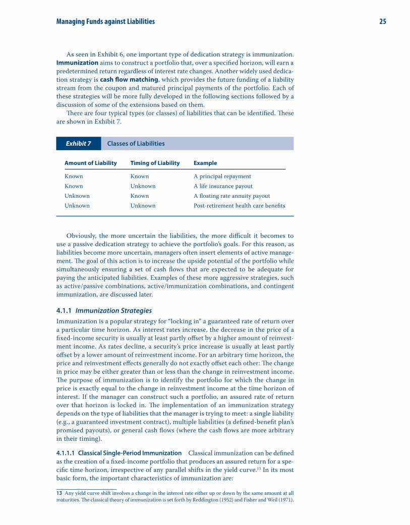


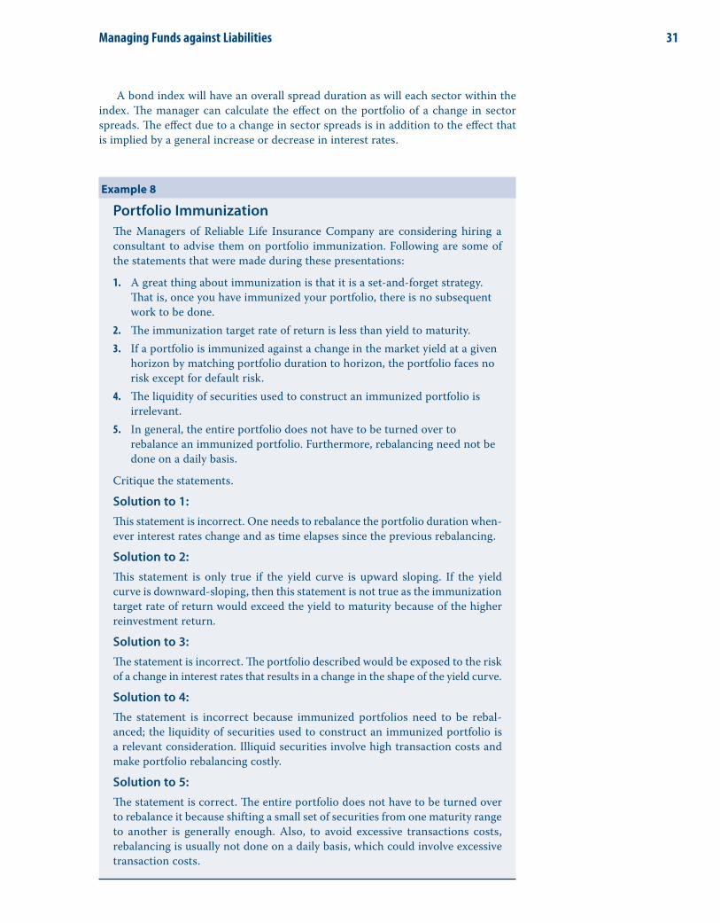


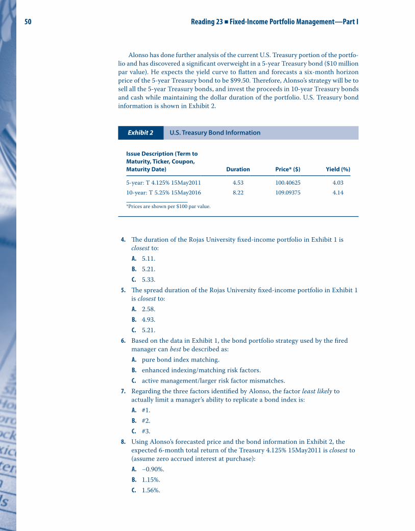


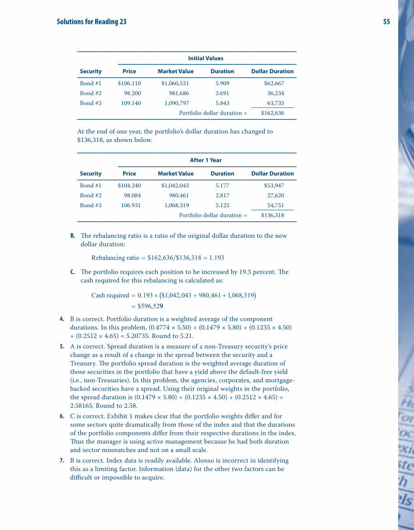


![Singer, Brian & Fedorinchik, Greg – Investment Leadership ... · Singer, Brian & Fedorinchik, Greg – Investment Leadership and Portfolio Management John Wiley & Sons, 2010, [Finance]](https://static.documents.pub/doc/80x56/5b4ca20e7f8b9acc378b48fc/singer-brian-fedorinchik-greg-investment-leadership-singer-brian.jpg)


