1 “Portfolio Risk Management Using Six Sigma Quality Principles” Abstract As the financial crisis of 2008 has revealed, there are some flaws in the models used by financial firms to assess risk. Credit, volatility, and liquidity risk were all inadequately modeled by supposedly sophisticated financial institutions employing dozens of financial engineers with advanced degrees. What went wrong? It is now becoming clear that some of the underlying assumptions of the statistical models utilized were seriously flawed, and interactive and systemic effects were ignored or improperly modeled. Correcting these modeling flaws is one approach to preventing a reoccurrence. However, another approach is suggested by Six Sigma quality programs used in manufacturing and service industries. Some basic tenets of the Six Sigma programs are directly applicable to improving risk management in financial firms and in portfolio design. These include the features of over-engineering, robust design, and reliability engineering. This paper will discuss the main features of Six Sigma quality programs, show how they can be applied to financial modeling and risk management, and demonstrate empirically that the Six Sigma approach would have provided an adequate safety margin at the actual daily one percent Value-at-Risk measure observed for the period from 1926 to 2011. Keywords: risk management, VaR, Black Swan event, Six Sigma, portfolio design Introduction In March of 2008 Bear Stearns was acquired by JP Morgan Chase after becoming insolvent. Bear Stearns had been considered one the best Wall Street firms in managing risk. Within a few months Lehmann Brothers had gone bankrupt, Merrill Lynch had been acquired by Bank of America, Wachovia merged with Wells Fargo, and Washington Mutual with JP Morgan Chase. American International Group (AIG) was bailed out by the federal government and many hedge funds have failed. What had caused so many prominent financial institutions to succumb in such a short time? The common explanation is sub-prime mortgages defaulting, but the real problem is much more fundamental—a failure of risk management. The no down-payment, no income verification mortgages issued by many reputable financial institutions may have started the problems, but they would not have spread worldwide without the explosive advance in securitization of these assets (Collateralized Debt Obligations or CDO’s) by financial firms and the high credit ratings assigned to them by the rating agencies Standard & Poor’s and Moody’s. The problems would probably not have grown to be a global financial crisis if so many other financial institutions had not purchased these risky assets including many banks in Europe and hedge funds around the world. Once the dominos began falling, liquidity dried up, and equity markets plummeted. The outcome became a financial crisis leading to a global recession which still continues.
Transcript
1
“Portfolio Risk Management Using Six Sigma Quality Principles”
Abstract
As the financial crisis of 2008 has revealed, there are some flaws in the models used by
financial firms to assess risk. Credit, volatility, and liquidity risk were all inadequately
modeled by supposedly sophisticated financial institutions employing dozens of financial
engineers with advanced degrees. What went wrong? It is now becoming clear that
some of the underlying assumptions of the statistical models utilized were seriously
flawed, and interactive and systemic effects were ignored or improperly modeled.
Correcting these modeling flaws is one approach to preventing a reoccurrence. However,
another approach is suggested by Six Sigma quality programs used in manufacturing and
service industries. Some basic tenets of the Six Sigma programs are directly applicable
to improving risk management in financial firms and in portfolio design. These include
the features of over-engineering, robust design, and reliability engineering. This paper
will discuss the main features of Six Sigma quality programs, show how they can be
applied to financial modeling and risk management, and demonstrate empirically that the
Six Sigma approach would have provided an adequate safety margin at the actual daily
one percent Value-at-Risk measure observed for the period from 1926 to 2011.
Keywords: risk management, VaR, Black Swan event, Six Sigma, portfolio design
Introduction
In March of 2008 Bear Stearns was acquired by JP Morgan Chase after becoming
insolvent. Bear Stearns had been considered one the best Wall Street firms in managing
risk. Within a few months Lehmann Brothers had gone bankrupt, Merrill Lynch had
been acquired by Bank of America, Wachovia merged with Wells Fargo, and Washington
Mutual with JP Morgan Chase. American International Group (AIG) was bailed out by
the federal government and many hedge funds have failed. What had caused so many
prominent financial institutions to succumb in such a short time? The common
explanation is sub-prime mortgages defaulting, but the real problem is much more
fundamental—a failure of risk management.
The no down-payment, no income verification mortgages issued by many reputable
financial institutions may have started the problems, but they would not have spread
worldwide without the explosive advance in securitization of these assets (Collateralized
Debt Obligations or CDO’s) by financial firms and the high credit ratings assigned to
them by the rating agencies Standard & Poor’s and Moody’s. The problems would
probably not have grown to be a global financial crisis if so many other financial
institutions had not purchased these risky assets including many banks in Europe and
hedge funds around the world. Once the dominos began falling, liquidity dried up, and
equity markets plummeted. The outcome became a financial crisis leading to a global
recession which still continues.
2
How could these sophisticated financial institutions have been so wrong in their
assessment of credit and market risk? After all, many had invested millions of dollars in
risk modeling and believed that they had a good handle on risk management. With
increasing power of computer hardware and software, firms were able to build
complicated models using advanced statistical techniques and Monte Carlo simulations.
To develop these models they hired dozens of mathematicians, statisticians, physicists,
and computer scientists, and a new profession was created—the financial engineer. Very
few top executives responsible for risk management likely understood these models, but
they confidently used them to take ever-riskier positions to increase profitability, often
driven by competitive pressures. Short-term oriented compensation schemes fostered
excess risk-taking in many of these financial firms. Few believed that there were any
flaws in the models.
Clearly there were some critical elements in the risk models that caused them to fail when
they were most needed. In the next section we will examine some of the deficiencies of
these models. In subsequent sections Six Sigma quality programs will be explained and
it will be shown how the process and methods of Six Sigma can be applied to financial
instrument and portfolio design. An empirical example using returns data from T-Bills,
NYSE/AMEX and NASDAQ over a period of 49 years from 1963 to 2011 will be
presented. The case will be made for robust portfolio design and reliability engineering
used as the way to achieve robustness. The last section draws some conclusions.
Flaws in Risk Modeling
The most commonly used model to measure risk is the VaR or Value-at-Risk. It is based
on the Gaussian or normal probability distribution widely used for many applications in
business, science, education and other fields. By specifying an acceptable confidence
level for unlikely occurrences (such as the probability of a 5% chance of a 30% fall in the
price of a stock), risk managers could feel comfortable that these rare events had such a
low probability they could be neglected. A three sigma confidence level indicates a 0.3
percent chance (3 in 1000) of the event occurring. The probabilities were based on
historic price and volatility data for various types of assets. This stochastic approach to
risk management seemed safe and reasonable as long as the underlying assumptions of
the statistical model are valid. However, as recent events have dramatically illustrated
some of the underlying assumptions are clearly not valid.
The most serious flaw in the VaR models is the assumption that the underlying
distribution is Gaussian. There is much evidence that many asset prices follow a
distributive pattern that is not a Gaussian, or normal, distribution (Mandelbrot 1963,
Fama 1965, Kon 1984, Chen 2015). This means that rare events such as a sharp fall in a
market occur much more frequently than a normal distribution would predict. With the
Gaussian model an event like the September 29, 2008, drop in the DJIA of 777 points or
7% had a probability of 1 in a billion, a probability so small that it can be neglected and
is essentially unpredictable with conventional forecasting models (Mandelbrot and
Hudson, 2004). These Black Swan events happen much more often than any Gaussian
3
model can predict. Taleb (2007) defines a Black Swan event as one that is rare, has an
extreme impact, and is retrospectively (though not prospectively) predictable. The 2008
crash can be seen as a Black Swan event that the models did not predict. Since a Black
Swan event cannot be predicted, what can a risk modeler do? Suggestions will be offered
below on how to mitigate the consequences of such events.
VaR models assume that the distribution is symmetric. There is substantial research
evidence that this assumption is invalid for many asset prices and markets. Risk
preferences are often asymmetric towards upside and downside risk. Arditti (1967) show
that investors prefer positive to negative skewness in returns. Mitton and Vorkink (2007)
find that a sample of investors in a discount brokerage firm hold less than optimal
portfolios according to mean-variance theory with lower Sharpe ratios and positive
skewness. The multivariate normal assumption of symmetry is therefore suspect.
Gaussian-based risk modeling assumes a stationary distribution with no shift of the mean.
In reality, for a variety of reasons both economic and psychological, the mean of a
distribution of asset prices may suddenly shift (economists call this a regime change),
leading to a greater area in one tail of the distribution than previously forecast. Such a
mean shift can increase dramatically the probability of an unlikely event that might have
seemed remote before, such as a sudden, large fall in a market. The stationarity
assumption is also empirically suspect (Considine 2008).
Another flaw in conventional VaR models is the volatility variable utilized. This is the
standard deviation (sigma) from the normal distribution based on historic volatility.
There are three problems with this approach. First, if the underlying distribution (the
normal) is not the correct one, then standard deviation as a measure of variability will
also be wrong (Haug and Taleb 2008). Second, historic volatility may not be a good
representation of future volatility. If in fact the distribution is leptokurtic, then a
variability measure based on the normal distribution will seriously underestimate the
probability of an extreme movement. Third, volatility is not stationary (Chen 2015). In
times of market stress, volatility can spike dramatically. Many risk management models
were calibrated to 2003-2006 volatility which was very low by historical standards
(Varma 2009). There is also evidence for volatility clustering and intra-day volatility
being much greater than day-to-day volatility which is typically used in risk modeling
(Basu 2009).
A further problem with conventional risk modeling is the assumption of independence of
various markets and assets. This is clearly not a valid assumption in times of market
stress as they become much more correlated as recent events demonstrate. Heightened
volatility in one market quickly spreads to another increasing the covariance of the
markets. Under such conditions of contagion, diversification by country or asset class
does not provide the expected protection. Correlations among assets categories and
markets have been shown to be non-linear (increasing in times of market stress) and
asymmetric (differing between rising and falling markets). (Varma 2009) As the recent
financial crisis has demonstrated, a sudden loss of liquidity in markets and rapid changes
4
in credit-worthiness of counterparties are examples of systemic risk. These risks were not
well modeled in VaR-based risk management systems.
VaR models are typically validated by backtesting against historical data. This presents a
set of problems that make their use suspect. The asset prices and markets used, the
historical period selected, and measurement errors as well as model misspecification all
can lead to improper validation of the VaR models used by financial institutions.
Escanciano and Pei (2012) and Gabrielsen, et al (2012) discuss these issues and propose
better methods for backtesting of VaR models.
These same deficiencies underlie much of modern finance theory. Mean-variance
portfolio optimization (Markowitz, 1952), the Capital Asset Pricing Model (Sharpe,
1964), and the Black-Scholes Option Pricing Model (Black and Scholes, 1973) all are
based on the Gaussian probability distribution. If this is not the correct distribution for
modeling asset prices, or variance is incorrectly measured, or mean shifts occur and
markets are interdependent, then these models must be suspect as well. Yet many asset
pricing and investment decisions are made based on these models. This also contributed
to the recent financial crisis (Haug and Taleb 2011, Varma 2009).
All of these deficiencies in conventional risk modeling (non-normal distributions, mean
shifts, volatility measures, and lack of independence) are not easily overcome with
standard statistical techniques. One can use a leptokurtic distribution like the Student’s t,
model regime changes, attempt to find better measures of prospective volatility, and
model interdependencies between markets, but there are disagreements about appropriate
ways to accomplish these improvements, and there are no standard methods. As Chen
(2015) notes “The problem is so severe that we may need to concede that the entire class
of problems best modeled by fat-tailed distributions transcends the category of risk,
where probability is quantifiable, and enters the distinct category of uncertainty, where
probability is unquantifiable.” Another approach may be needed in such a situation, and
one that holds promise to improve risk modeling is Six Sigma, which is widely used in
quality and process improvement programs in industry and services. This will be
discussed in the following section.
Six Sigma Quality Programs
Beginning in the 1980’s at Motorola Corporation, Six Sigma quality programs have
slowly spread through American manufacturing and recently have been applied in service
businesses like banking, hospitals, and even government. The basic idea behind Six
Sigma is to reduce variability in processes to improve quality and increase efficiency.
The rigorous application of statistical tools to targeted business processes has led to some
dramatic improvements. The most visible example of success with Six Sigma has been
General Electric Company which has used it widely in manufacturing and transactional
areas calculating the savings corporate-wide at $3 billion (Evans and Lindsay, 2008). A
key insight that underlies the Six Sigma philosophy is that as business processes and
products become more and more complex, a much higher level of internal quality is
5
needed. This leads to some methods of the Six Sigma toolkit being directly applicable to
financial modeling, which like manufacturing has become increasingly complex with
significant interactions among variables.
The name Six Sigma refers to six standard deviations from the mean. This signifies a
level of quality equal to three defects per billion opportunities based on the normal
distribution. To many observers this seems like an unnecessarily high level of quality
that is not only unattainable but too expensive. However, when one considers several
characteristics of products and processes as well as how Six Sigma programs are carried
out, these objections are not valid. The cost criticism can be rejected in some cases based
on the experience of companies like GE that have found that the savings from reduction
in defects (i.e. scrap, rework, warranties, etc.) and improved process efficiency far
outweigh the costs of implementing the program (Evans and Lindsay, 2008).
The criticism of being an unrealizable goal has also been disproved by companies such as
Motorola, GE and others that have attained six sigma quality levels in both
manufacturing and transactional areas like bill processing. But whether such a high
standard is really needed is a further issue. One consideration is an issue neglected in
VaR models discussed in the previous section. This issue is the probability of mean
shifts in the process being considered (due to such factors in production processes such as
variations in machine and human performance over time). Six Sigma programs typically
assume a 1.5% shift in the mean is possible and adjust for this by seeking a higher sigma
level than would otherwise be needed with no such mean shift. With a 1.5% mean shift,
Six Sigma quality becomes three defects per million opportunities (rather than per
billion), and this is commonly the statistical quality level assumed in a Six Sigma
program where the mean is assumed likely to shift. In investment portfolios mean shifts
of the return distribution can be expected to occur due to contagion causing increasing
covariance in financial crises.
For a product with multiple parts, the reliability of the product is a multiplicative function
of the reliability of its component parts. For example, in a product with a thousand parts,
each one having a reliability of six sigma, the overall reliability of the product is about
three sigma (3 defects per thousand). Many products have more than one thousand
parts—a car has about 2000-3000 parts and a jetliner 200,000-300,000 parts and
components. Therefore, designing in very high levels of individual component
performance is essential to reliability of the finished product. This suggests one
fundamental aspect of Six Sigma that has direct applicability to financial modeling—
what we might call over-engineering. The more assets an investment portfolio contains
and the more complex these assets may be (i.e. derivatives), the greater the possibility of
severe drawdown in a financial crisis.
Rather than assume that we are correctly modeling the underlying distribution with the
Gaussian, Six Sigma builds in a margin of error for fat tails. Although Six Sigma
statistical processes are also based on the normal distribution, the high levels of sigma
applied provide a much greater safety margin than the normal three sigma assumption of
VaR. Correctly specifying the underlying distribution becomes much less critical in a Six
6
Sigma process--it does not matter very much when the probability of a tail event is so
small.
Mean shifts, another weakness of financial models, is allowed for explicitly in Six Sigma
by targeting a high level of standard deviations. Even if the mean does shift, as it is
assumed likely to do, in Six Sigma the confidence level is still very high. This again
illustrates the concept of over-engineering the process to account for rare but expected or
unexpected occurrences.
In a similar fashion, the proper measurement of variability in a process is also less
critical. A machine’s variability may be more accurately captured by historic data than
an asset price, but again the margin of error for an incorrect assessment is much greater
with a six sigma confidence level. Once more we find the concept of over-engineering
being applied.
The fourth weakness of traditional financial models is the interactive effects between
financial instruments and markets. Six Sigma quality programs face a similar problem in
complex processes with many interacting variables. An example is a metal plating
process where temperature, humidity, fluidity, and other factors all affect process results.
Six Sigma has developed ways to analyze these interactive effects and determine the best
combination of variables to minimize process variation. These are part of the process of
robust design and include methods like Design of Experiments (DOE) and Design Failure
Mode and Effects Analysis (DFMEA). These and other methods for robust design will
be discussed in the next section.
Another element of Six Sigma that has applicability to financial risk modeling is
reliability engineering. This concept is used in product design where failure of one
component can lead to failure of others and even complete product failure. Especially
when components operate in series, it is essential to build in high levels of reliability and
use redundant systems as backup. An example is an auxiliary power or hydraulic system
on a airplane that kicks in if the main system fails. Design of financial products can also
take account of the interactive effects of the instruments and markets and attempt to build
in reliability. It would involve extensive stress testing and simulation of performance
under a variety of conditions. It could also involve using hedging instruments to add
resiliency. This concept will be considered in a subsequent section along with other
suggestions and a process for applying Six Sigma to the design of financial products.
First, though, let us examine if a Six Sigma approach to portfolio construction would
prevent massive drawdowns during financial crises.
7
Empirical Investigation: Can Six Sigma Give Us A More Realistic Measure of
Value-at-Risk? Example on Portfolio Construction and Results
Since the normal distribution is known to severely underestimate the tail probability
density of actual rates of returns, we cannot get a realistic measure of the Value-at-Risk
(VaR) that is computed based on the mean and standard deviation from a normal
distribution. A relatively easy and direct approach to resolve this issue is to amplify the
standard deviation used in the VaR calculation while still keeping the normal distribution
assumption. This is akin to fitting the tail of the actual distribution with a normal
distribution by inflating the standard deviation of the normal distribution. For example,
the one percent VaR is computed as: 𝐸(𝑅) − 2.33 × 𝜎. The essence of the Six Sigma
approach we propose here is to replace the actual standard deviation, 𝜎, by an amplified
version of this standard deviation, 𝜋 × 𝜎, where π is the multiplicative factor. Following
the standard Six Sigma approach, one would amplify the standard deviation six times (π
=6). Would this be adequate to give us a realistic measure of the one percent VaR and
thereby provide an adequate safety margin for actual outcomes? To address this
question, we analyze the distribution of actual daily portfolio returns for portfolios
constructed using stocks that were traded on NYSE/AMEX and NASDAQ over a period
of 49 years from 1963 to 2011. These portfolios are the value-weighted, equally-
weighted, S&P500, and Decile 1 through Decile 10 portfolios.
Description of Data
The data used in this study are the daily returns for stocks traded on NYSE/AMEX
/NASDAQ over the period from 1963 to 2011. These stocks are organized into portfolios
for our analysis. The value-weighted and equally-weighted portfolios contain all the
stocks that existed in each year. The weight of each stock in the value-weighted portfolio
is determined by the market capitalization of the stock relative to the total market
capitalization. The decile portfolios for each year are formed by grouping stocks into ten
portfolios based on market capitalization with each portfolio containing roughly the same
number of stocks. Each decile portfolio is also constructed using the value-weighted
method. Decile 1 contains stocks with the smallest market capitalization and Decile 10
the largest market capitalization.
Table 1 shows the number of stocks that are in each decile portfolio for each year from
1963 to 2011. The total number of stocks traded in NYSE/AMEX /NASDAQ reached a
peak of 9,520 stocks in 1997 and since then the number of stocks has reduced over time
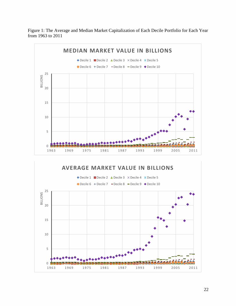
to 5,602 stocks in 2011. Figure 1 shows a plot of the average and median market
capitalization of each decile portfolio over time. For the largest decile portfolio, Decile
10, the average market capitalization is roughly twice its median market capitalization
value suggesting that within Decile 10, the market capitalization for the top half in this
decile is a lot larger than the bottom half.
(Insert Figure 1 here)
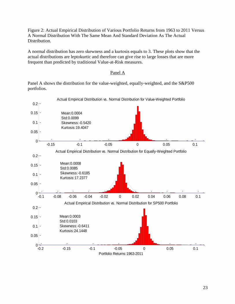
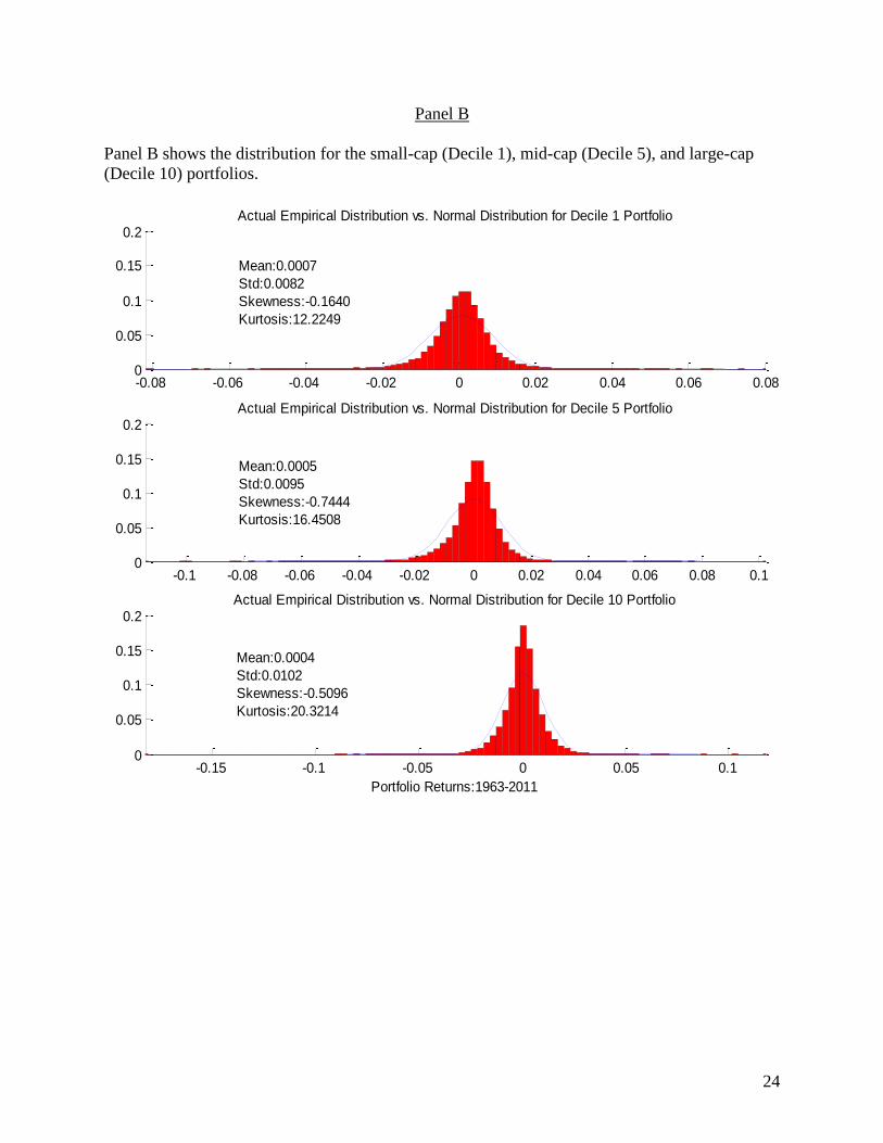
We pointed out at the start of this section that the normal distribution severely
underestimates the tail probability density of actual rates of returns. To provide a visual
8
illustration of this problem, we present Figure 2. Figure 2 compares the actual empirical
distribution of portfolio returns to a normal distribution with identical average return and
standard deviation as the actual distribution. The actual empirical distribution is
represented as a histogram and the normal distribution by a line in Figure 2. To save
space, we present the results for only the value-weighted, equally-weighted, S&P500,
Decile 1, Decile 5 and Decile 10 portfolios. In all cases we see that the actual
distributions are leptokurtic in comparison to the normal distribution. The kurtosis for a
normal distribution is 3 and the kurtosis for the actual distributions ranges from 12.22 to
24.14. It is therefore not surprising that the extreme losses that were encountered in
practice are much larger and more frequent than predicted by traditional VaR measures
that assume that returns are normally distributed.
(Insert Figure 2 here)
Next, we explain how we calculate the multiplicative factor in the six-sigma approach we
propose to address the problems in traditional VaR measures and discuss the results.
Calculation of the Sigma Multiplicative Factor
An easy and direct approach to resolve the problems in traditional VaR measures is to
amplify the standard deviation used in the VaR calculation while still keeping the normal
distribution assumption. In other words, we calculate the one percent VaR as 𝐸(𝑅) −2.33 × 𝜋 × 𝜎 where 𝜋 is the multiplicative factor. Following the standard Six Sigma
approach, one would amplify the standard deviation six times, that is set π =6. Would this
be adequate to give us a realistic measure of the one percent VaR and thereby provide an
adequate safety margin for actual outcomes? We present our results in Figure 3 and 4.
The actual values for the multiplicative factors are presented in Tables 2, 3, and 4. The
essence of our findings is that a multiplicative factor of “6” is adequate to compensate for
the higher likelihood of encountering extreme events in actual distribution.
To simplify our exposition, we will use t to identify a period that starts at t and ends right
before t+1. For instance, if the period is a year, then t could be Jan 1st, 1963 and t+1
would be Jan 1st, 1964. We begin by first calculating the empirical one percent VaR for a
given period, t, by sorting the returns in ascending order and then determining the cut-off
value, 𝑅∗𝑡, at the 1% level. We then calculate the multiplicative factors associated with
the ex-post and ex-ante theoretical VaR. In both cases, we need to determine the value of
the multiplicative factor, 𝜋, that is necessary for the theoretical VaR to match the
empirical VaR. The calculations are summarized by the following two equations:
Ex-Post Theoretical VaR: 𝜇𝑡 − 𝜋|𝑍𝛼|𝜎𝑡 = 𝑅∗𝑡 or
𝜋𝑡 =𝜇𝑡 − 𝑅∗
|𝑍𝛼|𝜎𝑡
Ex-Ante Theoretical VaR: 𝜇𝑡−1 − 𝜋|𝑍𝛼|𝜎𝑡−1 = 𝑅∗𝑡 or
𝜋𝑡 =𝜇𝑡−1 − 𝑅∗
|𝑍𝛼|𝜎𝑡−1
9
Note that R* is a negative value and |𝑍𝛼| is the z-score of the standard normal
distribution at the (1-α%) (e.g. α%=1%) cut-off of the left tail. For a 1% VaR, 𝑍𝛼 = 2.33.
The difference between the ex-post and ex-ante theoretical VaR calculation lies in what
we used as estimates for the average return, 𝜇, and standard deviation, 𝜎, in the
calculation. In the ex-post VaR calculation, we use the sample estimates for the average
return and standard deviation from period t; the same period used to determine the actual
empirical VaR. But in the ex-ante VaR calculation, we use the sample estimates for the
average return and standard deviation from the preceding period, which is (t-1). In other
words, we use the average return and standard deviation in the preceding period as a
forecast of the same variables in the current period. In managing the risk of actual
portfolios with VaR, we do not know in advance the actual average return and standard
deviation that are needed for calculating the VaR for the forward looking period and
therefore will have to forecast these values. Clearly our analysis for the ex-ante VaR case
employs a rather naïve forecasting method for forecasting the average return and standard
deviation. The point we want to demonstrate is whether the six-sigma approach could
indeed work in practice even with a naïve forecast of the average return and standard
deviation. If it works, then it would certainly work better with more sophisticated
forecasting method. Consequently, the results for the ex-ante case will be critical in
shedding light on the validity of the six-sigma approach.
The calculations above assume daily returns and the computation of VaR for a 1-day
horizon. For a h-day horizon VaR, the calculation of the multiplicative factor, assuming
returns are iid, becomes
𝜋(ℎ)𝑡 =(𝜇𝑡−1 − 𝑅∗
𝑡) × ℎ
|𝑍𝛼|𝜎𝑡−1 × √ℎ= √ℎ × 𝜋𝑡
The results for the ex-post VaR case are presented in Figure 3 and Table 2. Figure 3
shows that that the multiplicative factor for each portfolio consistently remains less than
3 over the 49 years from 1963 to 2011.
(Insert Figure 3 here)
This implies that if we have perfect forecast of the average return and standard deviation
for the period in which we want to compute the VaR, then using a multiplicative factor of
6 is more than adequate to compensate for the higher likelihood of encountering extreme
events in the actual distribution. Obviously, we cannot expect to have perfect forecast of
the average return and standard deviation in the future period. To better understand if the
six-sigma approach will be useful in practice, we repeat the analysis by using a naïve
forecast described earlier. The results for the multiplicative factor associated with naïve
forecast or what we called the ex-ante VaR case are presented in Figure 4 and Table 3.
(Insert Figure 4 here)
10
We see from Figure 4 that the values for the multiplicative factors rarely exceed 6 times
over the 49 years even with a naïve forecast of the average return and standard deviation.
To be more specific, Table 3 shows that the values for the multiplicative factor exceed 6
only once for some portfolios. This happened in 1987 for Decile 3, Decile 4, Decile 5,
Decile 6, and Decile 7 portfolios and their respective values for the multiplicative factor
are 6.70, 6.80, 6.78, 6.32, and 6.10. Even when the value for the multiplicative factor
exceeds 6, we see that it is not that much larger and it is still less than 7. Our results
suggest that the six-sigma approach provides a reasonable approximation of actual ex-
ante VaR measure.. In the next section, we apply the six-sigma approach to manage the
risk of various portfolios and compare the performance of the risk-managed portfolios to
that of a risk-free security.
Managing Portfolio Risk with the Six-Sigma Approach
We focus now on illustrating how to use the six-sigma approach to manage the risk of
these risky portfolios: value-weighted, equally-weighted, S&P500, and Decile 1 to Decile
10. We construct our hypothetical portfolio (C) to be a two asset one: 1) a risk-free asset
(T-Bill) and 2) a risky portfolio (one of the risky portfolios mentioned above). Our target
investor in this combined portfolio (C) is one who wishes, with specified certainty that
his holding will not fall by more than the desired % during his defined target period.
Using the six-sigma approach described in the previous section, a one percent VaR is
defined as 𝜇𝑐 − 2.33 × 6 × 𝜎𝑐.
In our two asset portfolio construction, let 𝜇𝑓, 𝜇𝑐 and 𝜎𝑐 (𝜇𝑝 𝑎𝑛𝑑 𝜎𝑝) represent the risk-
free rate of return, the expected daily return and standard deviation of the combined
portfolio (risky portfolio) and w be the investment weight in the risky portfolio.
Assuming zero correlation between the riskless and risky portfolios, the expected daily
return and standard deviation of the combined portfolio can be written as:
𝜇𝑐 = 𝑤𝜇𝑝 + (1 − 𝑤)𝜇𝑓
𝜎𝑐 = 𝑤𝜎𝑝
For the combined portfolio to meet a certain VaR requirement; for example to have a (1-
α) probability of suffering a loss no larger than ∅∗(where ∅∗ is a negative value) within a
day, we will need
𝜇𝑐 − 𝜋|𝑍𝛼|𝜎𝑐 ≥ ∅∗
Substituting into this equation the expressions for 𝜇𝑐 and 𝜎𝑐 and focusing on the
boundary case lead to
𝑤𝜇𝑝 + (1 − 𝑤)𝜇𝑓 − 𝜋|𝑍𝛼|𝑤𝜎𝑝 = ∅∗
𝑤(𝜇𝑝 − 𝜇𝑓 − 𝜋|𝑍𝛼|𝜎𝑝) = ∅∗ − 𝜇𝑓
𝑤 =∅∗ − 𝜇𝑓
(𝜇𝑝 − 𝜇𝑓 − 𝜋|𝑍𝛼|𝜎𝑝)
11
To compute 𝑤𝑡 at t, given that we haven’t observed the expected return and standard
deviation at t, we will assume that these values can be forecasted by the estimates for 𝜇𝑝,
𝜇𝑓, and 𝜎𝑝 at (t-1). 𝜋𝑡 is set to 6 in the six-sigma approach and 𝑍𝛼 is equal to 2.33 for a
1% VaR. Since ∅∗ by definition is a negative number:
𝑤𝑡 =∅∗ − 𝜇𝑓𝑡−1
(𝜇𝑝𝑡−1− 𝜇𝑓𝑡−1
− 𝜋𝑡|𝑍𝛼|𝜎𝑝𝑡−1)
The calculations above assume daily returns and the computation of VaR for a 1-day
horizon. For an h-day horizon VaR, the calculation of the weight, 𝑤𝑡, assuming returns
are iid, becomes
𝑤𝑡 =(∅∗ − 𝜇𝑓𝑡−1
) × ℎ
[(𝜇𝑝𝑡−1− 𝜇𝑓𝑡−1
) × ℎ − (√ℎ × 𝜋𝑡)|𝑍𝛼| (𝜎𝑝𝑡−1× √ℎ)]
𝑤𝑡 =∅∗ − 𝜇𝑓𝑡−1
(𝜇𝑝𝑡−1− 𝜇𝑓𝑡−1
− 𝜋𝑡|𝑍𝛼|𝜎𝑝𝑡−1)
which is the same as the 1-day result.
The equation above allows us to determine the weight, 𝑤𝑡, to allocate to the risky
portfolio and the riskless asset (1-𝑤𝑡) so that our combined portfolio will have a 1% VaR
that is equal to ∅∗. In our simulation, the portfolios were rebalanced annually to have a
one percent VaR that is equal to 10% over a one-day horizon. That is, we set ∅∗ to 10%
and we set the weight at the beginning of each year from 1963 to 2011 to the value
derived from the equation for 𝑤𝑡. This means that for each year we are constructing a
portfolio that 99 percent of the time will not lose more than 10% in value in the next day.
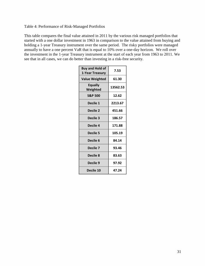
Table 4 shows the final value attained in 2011 by the various risk managed portfolios that
started with a one dollar investment in 1963. We see that in all cases, we can do better
than investing in a risk-free security.
(Insert Table 4 here)
Applying a Six Sigma Approach to Portfolio Risk Management
The major goal of a Six Sigma Quality Program is to reduce process variability to
improve product quality and reduce cost. The major goal of portfolio management is to
maximize a return to risk tradeoff. In essence they are the same objective—to get the
best results (return/quality) with the lowest cost (risk/cost). Six Sigma quality programs
emphasize a process approach to improving system reliability and performance. A
process approach stresses the sequencing and interactive effects in a system rather than
compartmentalizing the steps and activities. As was discussed above, the failure of risk
managers to account for systemic risks in investment portfolios contributed to the
12
financial crisis. The most widely used framework is the DMAIC process developed at
General Electric which includes the following steps: Define Measure, Analyze, Improve,
and Control (DMAIC). This same approach is applicable to portfolio design for financial
instruments and risk management systems for these portfolios. In this section we will
discuss how the DMAIC process can be used by financial firms to better design
investment products and control for risk, and, in the subsequent section, create a simple
example to illustrate how the process can work.
The first stage in applying the DMAIC process to portfolio design is to Define the types
of financial products to be considered in terms of the desired return to risk profile, the
types of instruments that can be considered, and the investment horizon. These of course
should be determined by top management of the firm, not by the quant’s developing the
products. Without these parameters clearly defined, financial engineers will not have
clear guidance in terms of the products they should develop. As the recent financial crisis
illustrates, this failure to have clear goals and constraints led to some products being
offered that were not well thought out and introduced a high level of unexpected and
undesired risk. Managers who did not understand the instruments because of complexity
approved these products with disastrous consequences.
The second step in the DMAIC process is to Measure. In a manufacturing process this
would normally involve collecting statistical data and finding process capabilities. Using
statistical control charts is common in industry to measure whether a process is
operationally under control and when it may be deviating from the norm. This can
provide a warning to the production staff that a process is going out of control and
corrections can be made before defects are produced The analogue in financial product
design would be to perform statistical tests and simulations using historical data to
determine the probability distributions of the instruments and markets. SPC might then
be utilized to indicate when these instruments or markets are deviating significantly from
their historical performance. An example of this can be found in the use of statistical
control charts to predict the bubble in the U.S. housing market in the first decade of this
century (Berlemann, et al, 2012).
Another goal is to ascertain how the instruments perform independently and together in a
portfolio. More advanced measurements would attempt to find the systemic effects on
the portfolio of liquidity and credit crises. This was a deficiency in the design of many of
the financial products that imploded in 2007 and 2008 such as CDO’s. A process
capability study determines the distribution of results of a machine or process in terms of
a density function (usually the normal distribution) to see if it can meet design
specifications. For a financial instrument this would involve finding the distribution of
returns over a period. For multiple instruments these can be analyzed with multivariate
regression and simulation studies to determine covariance and interactive effects. This
data will be essential for the next step in the process.
The third stage of the DMAIC process is to Analyze. For financial products this could
involve the technique called Design of Experiments (DOE). This method has been used
in manufacturing for many years to determine interactive effects in processes. As noted
13
above, interactive effects between financial instruments such as varying and asymmetric
correlations were poorly understood and modeled. DOE provides a tool to analyze these
kinds of influences on an investment portfolio. It involves a well-defined set of statistical
techniques to vary several variables simultaneously and see the combined effect on
performance of the process. For financial instruments this could be done by simulation
methods. For example, various asset categories could be combined in a systematic way
in hypothetical portfolios to see how they perform under differing market scenarios.
These interactive effects are a key element in another portion of analysis of portfolios
called stress testing. The systemic effects of disappearing market liquidity and rapidly
changing credit-worthiness on portfolios were poorly modeled in the recent crisis. Stress
testing using DOE and simulations can provide valuable insight into how investment
portfolios will respond under different economic and market scenarios.
Another tool from Six Sigma that may have some at least conceptual significance for
designing financial portfolios is Design Failure Modes Effects Analysis (DFMEA). This
technique is a systematic process of recording and analyzing failure of a product to meet
specifications. The objective is to understand the most frequent causes of failure and
why they occurred. This approach has been very successfully applied in the airline
industry where every crash is carefully analyzed to find the cause, and then modifications
to equipment and/or training are required by regulatory authorities. The result has been
continually improving air flight safety. Applied to portfolio design this would involve
determining why particular instruments did not perform as expected in terms of return
and risk. There is certainly a wealth of data from the last several years to perform this
kind of analysis. It will be critical to the design of better portfolios to understand why so
many failed in the financial crisis. Of special interest will be examining the interactive
and systemic effects in these portfolios. Andrew Lo (2015) has proposed such an
approach to investigating financial “accidents” such as market crashes to improve risk
management and reduce drawdown risk in investment portfolios.
To Improve is the next step in designing financial products by the DMAIC process. Here
a couple of techniques from the Six Sigma tool box can be useful. The first of these is
reliability engineering. Reliability engineering involves designing products to be robust
under difficult operating conditions. This is accomplished through several techniques
including standardization and redundant systems as well as the previously discussed
DOE. Standardization tends to make physical products more robust because of fewer
number of parts reducing complexity and interactive effects and the streamlining of
assembly and testing improving quality and reliability. Applied to financial products the
analogue would be to use established financial instruments that have a track record of
performance under different market conditions rather than new and customized
instruments. It will be difficult to construct a low-risk portfolio with many new and
bespoke instruments where the correlations and interactive effects are unknown.
Redundancy is an essential element in complex products to assure reliability. This can
take the form of parallel systems that backup the primary system in case of failure. In the
case of financial products this could be achieved by the use of financial hedges that will
offset any opposite movement in the underlying instrument. The concept of portfolio
14
insurance is relevant here. There are various ways to achieve this in an investment
portfolio by taking offsetting long and short positions and the use of options. A common
hedge is to take out-of-the-money puts to hedge against a large market drop. For hedging
against counterparty risk, Credit Default Swaps (CDS) can be used. CDS’s contributed
to the recent financial crisis because of the huge volume outstanding and their lack of
transparency. They were undoubtedly being used as a speculative instrument rather than
a hedge by many of the participants, but can be an effective hedge against credit risk if
used properly.
The last stage of the DMAIC process is to Control. Although risk management issues
should be considered throughout all five steps in the process, they are the main focus of
the last stage for financial products. The most important part of the control process is
assigning clear-cut responsibility for this activity. It should be at a high enough level in
the firm to have real control which was a problem with some of the financial firms most
impacted by the recent crisis where control responsibility was diffuse and ineffective.
Control also involves frequent reporting of essential information and separation of the
trading, sales, and reporting roles. Compensation systems should not encourage excessive
risk taking. Beyond these organizational issues portfolios should be continually subject
to stress testing as market and economic conditions change. This calls for individuals
with the requisite analytical skills.
The overall process for designing and controlling financial products following the
DMAIC model will allow for a more systematic and thorough process that has the
potential to prevent some of the problems which surfaced in the recent financial crisis.
The ad hoc and diffuse nature of risk management in many financial firms was revealed
during this crisis, and a more integrated and rational process is clearly called for.
Relevance of Model to DMAIC
The model developed previously is a rather simple one; only two assets, one risk-free, are
utilized, and simplifying assumptions are made regarding volatility. From this starting
point of defining a model, a DMAIC-type process would allow for a better and more
efficient portfolio construction as well as better estimates of volatility. A brief suggestion
of how this process might unfold follows.
We measured the standard deviation of the risky asset as the observed volatility of the
S&P 500 over the prior period of estimation. This choice of using a simple measure of
prior volatility to estimate future volatility is one of convenience and ease of calculation.
Alternate forms of measurement, such as volatility implied by option pricing, could and
should be utilized.
Use of prior volatility is the first stage in the measurement process. The results can then
be analyzed to determine how well it performed and compared to alternative models.
The next step is improving the model. For example, to improve the measure of volatility,
we could test how reliable the estimate is. How well does past volatility predict future
volatility? Here we can design experiments (DOE) to test more reliable predictions of
15
future volatility may be achieved. Processes described elsewhere in the paper suggest
how more accurate measures of volatility might be constructed. The goal is to develop a
model that will estimate prospective volatility with a high degree of accuracy. .Another
improvement might be in designing in redundancy. This may be achieved through a
variety of techniques that we may characterize as portfolio insurance, to be discussed
later in the paper. Other aspects of the model could also be analyzed and improved as
tests are run, alternatives tried, and results compared.
The final stage in the DMAIC process is control which could require a dedicated
portfolio manager to oversee the portfolio and assure compliance with portfolio
requirements. Clearly, different portfolios, depending upon the objectives of its
investors, will require different approaches to risk management. These approached
should be carefully defined, as noted above.
We have indicated a few examples of how the process might yield a more robust method
of portfolio management with an objective of protecting the investor from unacceptable
downturns in the value of their portfolio. We now turn to applying methods of Six Sigma
to portfolio design.
Six Sigma Methods of Robust Portfolio Design
Robustness, or performing well under all market conditions, is certainly a desirable
quality in an investment portfolio and one in which many investment products were
clearly lacking in the recent financial crisis. This is also a major goal of Six Sigma
quality programs which attempt to design robust products and processes. Typically
financial managers may not have thought of robustness as a critical quality in their
products, but many may now begin to do so. Six Sigma provides a conceptual and
methodological approach to do this as the last section indicated. .
The financial crisis that began in 2007 affected many financial firms in commercial and
investment banking, hedge funds, private equity funds, and insurance companies. But
one major category of financial institution escaped the havoc. These are the
derivatives/futures exchanges throughout the world. Not one futures exchange
experienced distress in the crisis (Varma 2009). The reason for this is that derivative
exchanges apply, and have applied for years, over-margining of positions. The margins
that counterparties must maintain with the exchange are very conservative. The primary
approach to establishing margin requirements at most derivative exchanges is the SPAN
(Standard Portfolio Analysis of Risk) developed by the Chicago Mercantile Exchange
(CME) in 1988. SPAN calculates the potential worst-case asset loss based on several
price and volatility scenarios to set the margin. This conservative approach worked well
with the chaos in the global asset and credit markets in the face of a sudden increase in
volatility and correlation breakdowns. It is a financial equivalent of over-engineering.
As was mentioned previously, asymmetrical and non-normal distributions cannot be
modeled adequately using VaR techniques. Attempts have been made to improve upon
16
VaR which have some potential. Coleman (2014) and Chen (2015) suggest using the
Student’s-t to account for fat tails. Goh, et al (2009) recently developed PVaR for
Partitioned Value-at-Risk. Their method divides the asset return distribution into positive
(gains) and negative (losses) half-spaces. This generates better risk-return tradeoffs for
portfolio optimization than the Markowitz model and is useable when asset return
distributions are skewed or abnormal. Other adaptations of VaR methods include BVAR
which incorporates stochastic volatility and fat-tailed disturbances (Chiu, et al, 2015),
EVAR for Extended Value at Risk by Chaudhury (2011), WVaR for Worst-Case VaR (El
Ghaoui, et al, 2003), and AR-VaR for Asymmetry-Robust VaR (Natarajan, et al, 2008).
All of these methods deal with some of the weaknesses of the basic VaR approach but
present computational difficulties and do not deal with non-stationarity due to
interdependencies and systemic effects completely.
There are various approaches to stress testing of a portfolio involving VaR or
simulations. Basu (2009) compares different stress tests on the foreign exchange (FX)
market. He postulates that a good stress test has several characteristics. First,
hypothetical scenarios must be combined with historical data to capture the impact of
severe shocks that have not yet occurred. Second, the tests should be probabilistic to be
interpreted as a refinement of VaR techniques. The third requirement is that they be
simple enough to communicate to top management. Using these criteria he concludes
that VWHS or Volatility Weighted Historical Simulation (Hull and White 1998)
performs the best in terms of smooth changes in the risk estimates as the size of the shock
varies. VWHS dynamically adjusts volatility rather than using historic volatility in the
simulations resulting in a more current scenario analysis. It also better models the impact
of stress on short positions and captures volatility clustering and fat tails in a simple
framework.
Diversification across asset categories and countries can provide some degree of risk
mitigation in a portfolio, but this can break down as markets become more correlated in
times of market stress. Building portfolios to maximize returns and minimize volatility
using historical data and sophisticated models is essential in portfolio design. But to be
truly robust, the portfolio must be designed to have offsetting long and short positions.
This can be accomplished through several hedging methods that provide portfolio
insurance.
There are several persuasive reasons to insure an investment portfolio against large and
unexpected losses. The most obvious is the revealed weaknesses of VaR models to
protect against large losses. The flaws in the VaR models were discussed above and
include non-normal distributions with fat-tails and skewness and non-stationarity. This
leads to poor performance of these models, particularly in the short-run (Considine 2008).
The short-run orientation of financial markets has been attributed to “reputational
concerns” of investment managers who are more concerned with retaining funds in the
near term than in long run out-performance of the market (Malliaris and Yan 2009).
“Herding effects” contribute to this phenomenon as well they say.
17
Portfolio insurance methods include the use of offsetting long and short positions for
price and market risk. These positions can be costly in terms of return that is sacrificed to
reduce risk. Another hedging method is to use options. Far out-of-the-money options
can be used to insure against extreme price moves at a modest cost of the premium which
is low for such options. To reduce the premium cost further one can write an offsetting
option but, of course, must assume some risk to do so. Simulations by Goldberg, et al,
(2009) find that out-of-the-money put options reduce ES and coincident extreme losses.
To insure against counterparty risk, one instrument that can be used is the Credit Default
Swap (CDS). For a series of premium payments counterparty risk can be transferred to
someone else. This of course assumes that the CDS counterparty does not themselves
default which has turned out to be a problem in the recent credit crisis. Other methods of
portfolio insurance will probably be developed in reaction to recent events allowing for
further refinement of reliability engineering for investment portfolios.
Conclusions
Financial markets have dramatically changed in the last three decades due to a confluence
of factors making them more volatile and less predictable. These forces include
increasing integration and globalization of the equity, bond, foreign exchange, and
commodity markets resulting in greater correlation between markets and assets and much
faster and extreme contagion between them. Secularization and financial engineering
have produced more complicated financial instruments which are difficult to model,
especially under conditions of market volatility and contagion. Automated trading has
greatly increased the speed at which volatility spreads through the markets. These forces
make financial markets much more difficult to model and forecast. The need for a
“safety margin” in portfolio design to prevent extreme drawdowns has become clear after
the recent financial crises. Earlier in the paper our descriptive model demonstrates that a
Six Sigma type framework, using a multiplier, provides a reasonably accurate description
of how an “adjusted” VaR may be created that reflects actual ex-ante risk. Six Sigma
principles, which have proven themselves adept at preventing unwanted variance in many
processes in manufacturing and services, suggest an approach to portfolio design and risk
management than can deal with the uncertainty and unpredictability of modern financial
markets and provide a margin of safety for investors. How these principles can be
applied to robust portfolio design have been discussed in this paper.
Fractal models can mimic what happens in market crises (Mandelbrot and Hudson 2004)
They are able to represent graphically “wild randomness” after the fact but are not useful
for prediction (Considine 2008). By definition Black Swan events are unpredictable and
thus cannot be mathematically modeled (Taleb 2007). We are in the realm of Knightian
uncertainty, rather than risk, here and traditional risk management approaches cannot
prevent large losses during periods of market turmoil. Since these events can have
devastating effects on an investment portfolio, how can an investor or a firm prepare for
them? There is no way to completely prepare for an unpredictable event but one can
certainly mitigate its effects. In an investment portfolio this can be accomplished through
the Six Sigma methods outlined in this paper.
18
The Six Sigma process can be applied to the design of risk management systems. It
provides a structured approach to collect data, analyze it, and develop financial products
with an integrative plan-achieve-control structure as part of the process. The DMAIC
process outlined in this paper is one way to accomplish this. Three key concepts of Six
Sigma quality programs have direct applicability to design of investment portfolios.
These are the principles of over-engineering, robust design, and reliability engineering.
Over-engineering of a financial product involves combining different instruments that
provide a return-risk tradeoff that mitigates extreme tail events. If well done, the result is
a robust design for the portfolio that will be able to respond in predictable ways to both
expected and unexpected market shocks and survive Black Swan events. Reliability
engineering provides an extra layer of protection using portfolio insurance methods to
hedge for extreme events using options, Credit Default Swaps, and other instruments and
requires stress testing and simulation to build in reliability and robustness.
Complicating design of financial instruments are behavioral factors such as the “Persaud
Paradox” where a false sense of confidence arises because peers are all using the same
approach, such as VaR models (Persaud 2003). Overcoming this is a responsibility of
risk management, and a structured approach as suggested in this paper can help in that
regard. Other behavioral issues such as herding and overconfidence also contribute to the
inadequacy of risk models and risk management (Rizzi 2009). Greenbaum (2014) and Lo
(2015) offer some suggestions for risk management practices to overcome these cognitive
biases. Much more research needs to be done to incorporate behavioral factors into risk
modeling. The difficulty of doing this is another argument to over-engineer financial
portfolios to make them robust to unpredictable behavioral phenomenon in financial
markets.
References
Arditti, Fred D. 1967, “Risk and the required return on equity”, Journal of Finance,
22, 19-36.
Basu, Sanjay, 2009, “Stress testing for Market Risk: A comparison of VaR Methods”,
Available at http://ssrn.com/abstract=1370965
Berlemann, M., J. Freese, and S. Knoth, 2012, “Eyes Wide Shut? The U.S. House
Market Bubble through the Lense of Statistical Process Control”, CESIFO
Working Paper 3962. Available at http://ssrn.com/abstract=2165772
Black, F. and M. Scholes, 1973, “The Pricing of Options and Corporate Liabilities”,
Journal of Political Economy, 81(3), 637-654
Boucher, C., P. Kouontchou, and B. Maillet, 2011, “An Economic Evaluation of the
Model Risk for Risk Models”, Available at http://ssrn.com/abstract=1943605
Chaudhury, Mo, 2011, “Extended Value at Risk Measure (EVAR) for Market Risk”
McGill University Desautels Faculty of Management Working Paper, Available at
http://ssrn.com/abstract=1809801
19
Chen, James M., 2015, “The Promise and the Peril of Parametric Value-at-Risk (VaR)
Analysis”, Social Science Research Network (SSRN), available at
http://ssrn.com/abstract=2615664
Chiu, Ching-Wai, Mumtaz, Haroon, and Gabor, Pinter, 2015, “Forecasting with VAR
Models: fat tails and stochastic volatility”, Bank of England Working Paper No.
528, Available at http://ssrn.com/abstract=2612030
Coleman, Thomas, 2014, “Financial Risk Measurement and Joint Extreme Events: The
Normal, Student-t, and Mixture of Normals”, University of Chicago Working
Paper, Available at http://ssrn.com/abstract=2437672
Considine, Geoff, 2008, “Black Swans, Portfolio Theory and Market Timing:
12 comments”, Seeking Alpha, Article 64111, Available at http://seeking
alpha.com/article/64111
El Ghaoui, L., M. Oks, F. Oustry, 2003, “Worst-case Value-at-Risk and Robust
Portfolio Optimization: A Conic Programming Approach”, Operations Research,
51(4), 543-556
Escanciano, J.C. and P. Pei, 2012, “Pitfalls in Backtesting Historical Simulation VaR
Models”, Center of Applied Economics and Policy Research Working Paper,
Indiana University, Available at http://ssrn.com/abstract=2026537
Fama, Eugene, 1965, “The Behavior of Stock Prices”, Journal of Business, 47, 244-280