Companionwebage‐cum‐blog forPGP‐1Financial Marketsclass with2comments The result that variance of the market portfolioisaweightedaverage of covariance of the underlying stockswiththemarketisageneral result.Thispostfillsinthemathematical blanks. Diversi fiablevs.Non‐diversi fiableRi sk:TheMath ConsiderthevarianceofaMarkowi ꜩ portfoliocontaining assets: Nowif we let the weight of each asset in the portfolio to be the same, i.e. , and considerthe“averagevariance”as: and“averagecovariance”as: thentheaboveportfoliovariancesimpli fiesto: Portfolio Selection | A Matter of Course https://pgpfm.wordpress.com/category/portfolio-selection/ 1 of 17 10-09-2015 01:21
Transcript
Companion webage‐cum‐blog for PGP‐1 Financial Markets class
with 2 comments
The result that variance of the market portfolio is a weighted average of covariance of the underlyingstocks with the market is a general result. This post fills in the mathematical blanks.
Diversifiable vs. Non‐diversifiable Risk: The Math
Consider the variance of a Markowitz portfolio containing assets:
Now if we let the weight of each asset in the portfolio to be the same, i.e. , and
consider the “average variance” as:
and “average covariance” as:
then the above portfolio variance simplifies to:
Portfolio Selection | A Matter of Course https://pgpfm.wordpress.com/category/portfolio-selection/
1 of 17 10-09-2015 01:21
Then as , the portfolio variance converges to:
That is, as the number of assets in the portfolio go up, the variance of individual assets becomeunimportant, and its the covariance terms that dominate. This is just our diversification. Graphicallythis can be represented as:
Diversification (Click on the figure to zoom; Source: Brealey‐Myers, 9th Ed.)
Unique Risk (or alternatively, Diversifable Risk, or Unsystematic Risk, or Idiosyncratic Risk) is the“average variance” of the individual assets.
As number of assets in the portfolio increase, this “average variance” tends to zero. The only risk, then,that matters is the one that remains after diversification has done its work. And this is just the averagecovariance between all assets in the portfolio. This is called Market Risk (or alternatively, SystematicRisk, or Undiversifiable Risk). And accordingly, the covariance of an asset with the market portfolio iscalled its market risk.
The fact that portfolio variance after diversification is just the weighted average of covariance betweenassets can be seen by first noting that:
Since the expectations add up, we can take out the summation sign outside the expectation, and itfollows that:
Portfolio Selection | A Matter of Course https://pgpfm.wordpress.com/category/portfolio-selection/
2 of 17 10-09-2015 01:21
That is the covariance of any asset with the market portfolio is nothing but the weighted average of itscovariance with all other assets in the portfolio.
Next, note that we can write:
(If you are looking for the variance terms, note the change in the limits in the summation operator, andrecall that )
Then if we substitute our result that , we see that:
That is the variance of the market portfolio is just the weighted average of the covariance of all assets inthe portfolio with itself. Again, this result is important enough to warrant a separate ‘box’:
If you notice, what we have done is essentially given a proof that covariances add up.
To see this, recall from your basic probability theory that for any three random variables, and :
.
If we let , and use the fact that , it immediately follows that
Our proof above is just a generalization of this result. Combine this with our observation that in thelimit individual variances (unique risks) disappear and we have our economic result that:
Moral of the Story 4: The risk of an individual asset is determined not by its individual variance, butby its covariance with the market portfolio, because the diversifiable/unique/idiosyncratic risk can
Portfolio Selection | A Matter of Course https://pgpfm.wordpress.com/category/portfolio-selection/
3 of 17 10-09-2015 01:21
be diversified away.
Written by Vineet
September 3, 2015 at 9:19 am
Posted in Diversification, FM, Portfolio Selection
Tagged with Diversification, FM‐2, Portfolio Theory, Session 9
leave a comment »
Enjoy!
Written by Vineet
August 29, 2015 at 6:09 am
Posted in FM, Portfolio Selection, Stories
Tagged with FM‐2015‐16, History, Interview, Markowitz, Stories
Portfolio Selection | A Matter of Course https://pgpfm.wordpress.com/category/portfolio-selection/
4 of 17 10-09-2015 01:21
with 3 comments
At this stage, having introduced the new straight line efficient set, we are all but there to our finaldestination. So, let’s step back a bit and try and understand the larger picture.
In the beginning was the efficient frontier. Markowitz gave us that. Efficient frontier describesthe maximum possible expected return for any given amount of risk from the portfolio of available assets. Oralternatively, the minimum amount of risk that one must live with for any given amount of expected return.
As a first step, we moved from individual assets to portfolios that lay on the efficient frontier. When wedid that implicitly the x‐axis (labeled as risk/standard deviation) then became the risk of the portfolio(and not the risk of the individual assets). There should be no cause for this confusion, but no harmemphasizing it nonetheless – the right risk to consider is the risk of the portfolio and not the individualasset.
Moral of the Story 1: When we consider the efficient frontier the relevant quantities to considerare portfolio risk and portfolio expected return.
Then, of course, Tobin came along and introduced a risk free asset in the Markowitz world, and he saidwe could ignore all other points on the frontier except the tangency one – because everybody wouldhold some proportion of only the tangency portfolio (as all other points even on the envelope arenow inferior), and the line connecting the return from the risk free asset and the tangency
portfolio offers the best possible combinations of portfolio risk and expected return. Remember, theoperative word here is portfolio.
This gave us our revised efficient set as:
(Click on the figure to zoom.)
The equation of the new efficient set immediately follows (it’s a linear line with intercept at and
slope ) as:
Portfolio Selection | A Matter of Course https://pgpfm.wordpress.com/category/portfolio-selection/
5 of 17 10-09-2015 01:21
…
What is the tangency portfolio ?
Having said that all investors should hold the tangency portfolio , the next thing to understand isthe meaning of this tangency portfolio. By saying that all investors should hold , what we areessentially saying is that investors would demand only combinations of portfolio and the risk‐freeasset. (Holding any other risky portfolio other than is inefficient.) This is the demand side of theproblem. What is the supply side? The supply side is just all the assets that exist in the market.
And by now you would know enough of microeconomics to understand that equilibrium requires thatdemand be same as supply. That is, assets demanded in the portfolio must exactly equal thesupply of each asset in the market. And the supply of each asset in the market is given by its marketcapitalization. So, in equilibrium all assets must be held in in exactly the same proportion astheir market capitalization. That is, in percentage terms weight of assets in the total marketcapitalization and in the portfolio must be the same.
Consider the case where you run your Markowitz optimizer and find that that weight of a particularasset, say is . Is that possible? Mathematically, of course, yes. But what about economically?Let’s try and understand this.
Saying that the weight of an asset in the Markowitz portfolio is is saying that no investorwants to hold the asset. If no investor wants to hold that asset, but the asset exists in the marketthen we have a state of disequilibrium. And what happens in a state of disequilibrium? Prices adjust.So, if no wants to hold an asset, its price will drop. Once the price starts to drop its expected return:
will rise. As the price starts to fall, and expected return starts to rise, investors would start to find thisasset more attractive. As its expected return rises even more, then when you re‐run your
Markowitz optimizer again, you’ll find that this asset has a non‐zero weight in the tangency portfolio . That is, all assets that exist in the market must be held. This brings us to another important lesson:
Moral of the Story 2: The tangency portfolio is nothing but the market itself!
As another example consider a situation where the Markowitz optimizer prescribes a weight of for an asset whose market capitalization is . What happens in that case? Well, now you know howto think about such disequilibrium situations. This is the case where the asset has more demand thansupply. When demand is more than supply, prices rise. As price rises, the expected return will fall. Asexpected return falls, the Markowitz optimizer will prescribe a lower weight to this asset and inequilibrium the price and the market capitalization of the asset would adjust to make the demandexactly equal supply. That is:
When one imposes equilibrium, the line passing through the tangency portfolio has a specific nameand it is called the Capital Market Line.
Note that at this stage, when we impose economic equilibrium, we have to necessarily assume thateverybody has the same information – things don’t quite work the same way otherwise. And thisbrings us to the last moral of the story for today:
Portfolio Selection | A Matter of Course https://pgpfm.wordpress.com/category/portfolio-selection/
6 of 17 10-09-2015 01:21
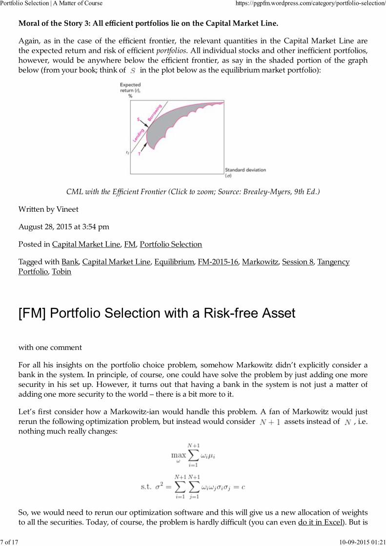
Moral of the Story 3: All efficient portfolios lie on the Capital Market Line.
Again, as in the case of the efficient frontier, the relevant quantities in the Capital Market Line arethe expected return and risk of efficient portfolios. All individual stocks and other inefficient portfolios,however, would be anywhere below the efficient frontier, as say in the shaded portion of the graphbelow (from your book; think of in the plot below as the equilibrium market portfolio):
CML with the Efficient Frontier (Click to zoom; Source: Brealey‐Myers, 9th Ed.)
Written by Vineet
August 28, 2015 at 3:54 pm
Posted in Capital Market Line, FM, Portfolio Selection
Tagged with Bank, Capital Market Line, Equilibrium, FM‐2015‐16, Markowitz, Session 8, TangencyPortfolio, Tobin
with one comment
For all his insights on the portfolio choice problem, somehow Markowitz didn’t explicitly consider abank in the system. In principle, of course, one could have solve the problem by just adding one moresecurity in his set up. However, it turns out that having a bank in the system is not just a matter ofadding one more security to the world – there is a bit more to it.
Let’s first consider how a Markowitz‐ian would handle this problem. A fan of Markowitz would justrerun the following optimization problem, but instead would consider assets instead of , i.e.nothing much really changes:
So, we would need to rerun our optimization software and this will give us a new allocation of weightsto all the securities. Today, of course, the problem is hardly difficult (you can even do it in Excel). But is
Portfolio Selection | A Matter of Course https://pgpfm.wordpress.com/category/portfolio-selection/
7 of 17 10-09-2015 01:21
it the best way to introduce a risk‐free asset in the Markowitzworld?
James Tobin, a colleague of Markowitz’s at the Cowles Foundation in the ’50s (and another NobelLaureate) argued that it’s not. And brilliant as his device was, we can easily see its impact in a twostock world.
In our familiar two stock world, let one of the assets be risk‐free, such that it’s rate of return is known‘today’ as with variance, of course, zero. Then, since of the assets is no more a random variable,
even the correlation between the two would also be 0. So, if in our set of equations:
we let we are left with:
That is, our Efficient Frontier in this case is simply a straight line connecting the rate of return from therisk‐free asset and the expected return from the asset , with slope If one could
assume that people could both borrow and lend at the same risk‐free rate, , then we could even
consider negative weights on the risk‐free asset, and extend the Efficient Frontier to the right (the“blue dots” in the graph below). So, if an investor would extremely risk‐loving he/she could borrowmoney from the bank and invest it in the second risky asset.
(Click on the graph to zoom.)
With this insight Tobin said that with the risk‐free asset in the world in the asset Markowtiz‐ianworld, we can just consider such straight lines emanating from the intercept on the ordinate (returnfrom the risk‐free asset ) and connecting with all the points on Efficient Frontier. That is, he said,
rather than re‐running the Markowitz optimizer, let’s only consider following straight lines connectingthe Efficient Frontier:
Portfolio Selection | A Matter of Course https://pgpfm.wordpress.com/category/portfolio-selection/
8 of 17 10-09-2015 01:21
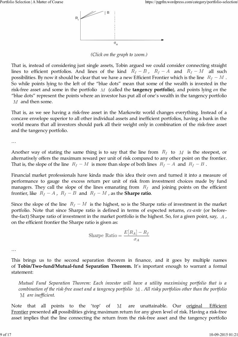
(Click on the graph to zoom.)
That is, instead of considering just single assets, Tobin argued we could consider connecting straightlines to efficient portfolios. And lines of the kind , and all such
possibilities. By now it should be clear that we have a new Efficient Frontier which is the line .
So while points lying to the left of the “blue dots” mean that some of the wealth is invested in therisk‐free asset and some in the portfolio (called the tangency portfolio), and points lying on the“blue dots” represent the points where an investor has put all of one’s wealth in the tangency portfolio
and then some.
That is, as we see having a risk‐free asset in the Markowitz world changes everything. Instead of aconcave envelope superior to all other individual assets and inefficient portfolios, having a bank in theworld means that all investors should park all their weight only in combination of the risk‐free assetand the tangency portfolio.
…
Another way of stating the same thing is to say that the line from to is the steepest, or
alternatively offers the maximum reward per unit of risk compared to any other point on the frontier.That is, the slope of the line is more than slope of both lines and .
Financial market professionals have kinda made this idea their own and turned it into a measure ofperformance to gauge the excess return per unit of risk from investment choices made by fundmanagers. They call the slope of the lines emanating from and joining points on the efficient
frontier, like , and , as the Sharpe ratio.
Since the slope of the line is the highest, so is the Sharpe ratio of investment in the market
portfolio. Note that since Sharpe ratio is defined in terms of expected returns, ex‐ante (or before‐the‐fact) Sharpe ratio of investment in the market portfolio is the highest. So, for a given point, say, ,on the efficient frontier the Sharpe ratio is given as:
…
This brings us to the second separation theorem in finance, and it goes by multiple namesof Tobin/Two‐fund/Mutual‐fund Separation Theorem. It’s important enough to warrant a formalstatement:
Mutual Fund Separation Theorem: Each investor will have a utility maximising portfolio that is acombination of the risk‐free asset and a tangency portfolio . All risky portfolios other than the portfolio
are inefficient.
Note that all points to the ‘top’ of are unattainable. Our original EfficientFrontier presented all possibilities giving maximum return for any given level of risk. Having a risk‐freeasset implies that the line connecting the return from the risk‐free asset and the tangency portfolio
Portfolio Selection | A Matter of Course https://pgpfm.wordpress.com/category/portfolio-selection/
9 of 17 10-09-2015 01:21
dominates all other possibilities. This is the new efficient frontier.
And now we can get rid of the original concave envelope, and we are left with just the
line. And a quick Google Image search gives us this nice little picture presenting different possibilitiescombining the risk‐free asset and the tangency portfolio:
[Click on the figure to zoom; Source: Wikipedia]
…
Post‐script
Needless to say, by definition, Sharpe ratio coincides with the slope of the line when the
investment manager chooses as the point on the frontier, i.e.:
Here is Nobel Laureate William Sharpe on the ratio that bears his name.
Written by Vineet
August 28, 2015 at 3:45 pm
Posted in Capital Market Line, FM, Portfolio Selection
Tagged with Bank, Capital Market Line, FM‐2015‐16, Markowitz, Session 8, Tangency Portfolio, Tobin
with 2 comments
With Markowitz having shown us that only expected return and variance of the gambles matter, weneed not restrict ourselves to considering 120‐80 kind of gambles with only two possible states of theworld. The only thing we need is estimates of expected return and variance of the gambles – and wecan study their combinations more generally. Let’s do that now.
…
Portfolio Selection | A Matter of Course https://pgpfm.wordpress.com/category/portfolio-selection/
10 of 17 10-09-2015 01:21
Consider two stocks and with expected returns , variances and
correlation between them. If we consider an investor with unit wealth, with amount invested in stock , and invested in stock then the portfolio expected return
and portfolio variance are easily obtained using some basic results from probability theory
as:
That is, as long as , portfolio risk (standard deviation) is always less than the risk (standarddeviation) of the linear combination of assets in the portfolio. This is called diversification.
It should be clear that the relationship between the portfolio weight in any asset and portfolioexpected return is linear, and that between portfolio weight and variance is quadratic. Our purpose,however, is to look at the trade‐off between expected return and variance of the portfolio.
We are lucky that the relationship between expected return and weight in any asset is linear so we caneliminate the weights and express expected return as a quadratic function of variance. The algebraicexpression is messy and lacks intuition, but for any given level of , it can shown (and as we did in theclass using Excel) that shape of the trade‐off is something like this:
Efficient Frontier: Two Assets
That is, the opportunities available to an investor is a concave envelope. And this envelope capturesthe trade‐off between expected return and risk available from the portfolio (geometrically speaking, it isa conic section – you can do the math and check which one!).
It should be clear that to a rational investor all the points below the minimum variance point should beinferior – as all those points represent a lower expected return for any given level of risk. That is, norational investor would prefer to choose a portfolio that lie below the minimum variance point.
The envelope traced by the upper arm of the curve above the minimum variance point is calledthe Opportunity Set (or Efficient Set or Efficient Frontier). This is the set of opportunities available toa rational investor given the securities available in the market.
Portfolio Selection | A Matter of Course https://pgpfm.wordpress.com/category/portfolio-selection/
11 of 17 10-09-2015 01:21
So, according to Markowitz all investors should choose one of the portfolios lying on the EfficientFrontier depending on their degree of risk aversion. So, if an investor is risk loving he/she shouldchoose one of the points on the top right end (high risk, high expected return), or if he/she isrisk‐averse choose one of the points on the bottom left part of the frontier, but never below the Frontier.
In a two‐asset world it was easy to visually identify the Efficient Frontier – but for an asset world,the Markowitz portfolio selection boils to solving the following Quadratic Programming problem:
or alternatively,
And how does the Efficient Frontier looks like for the case of assets? As expected, all the set ofopportunities available increase. But, importantly, luckily for us, Robert Merton showed thatthe Efficient Frontier retains the same concave shape whatever be the number of securities in themarket. In general, the shape looks something like the following (from your book):
Efficient Frontier: Multiple Assets (Click on the graph to zoom; Source: Brealey‐Myers, 9th Ed.)
Again, according to Markowitz, no investor should be on any point below the “pink line” (EfficientFrontier, traced by ABCD), i.e. in the shaded region, as all points on the curve ABCD offer a higherexpected return for any given level of risk / variance.
Given that expected utility is also a function of expected return and variance, by clubbing the twotogether Markowitz had solved the Portfolio Selection problem for a rational investor. So, if an investorwere risk‐averse he/she would choose a portfolio like C or D, and if one were risk‐loving then he/shewould choose a portfolio like B or A, but never anything below the curve ABCD.
…
Portfolio Selection | A Matter of Course https://pgpfm.wordpress.com/category/portfolio-selection/
12 of 17 10-09-2015 01:21
Special Cases
In the two‐stock world two special cases are interesting.
Consider two stocks and with expected returns , variances and
correlation between them. We had the following relationships for the portfolio variance from thetwo stocks:
1. Perfect positive correlation:
Setting doesn’t change the expected return , but simplifies the portfolio variance to:
i.e. the portfolio standard deviation is just a weighted average of the standard deviation of the twoassets. This is the case of zero diversification. Think of it this way. If the two stocks are perfectlypositively correlated, that is they move in lock‐step in the same direction all the time, it’s as if they arethe two same stocks
2. Perfect negative correlation:
Again, setting doesn’t change the expected return , but simplifies the portfolio variance
to:
While even in this case the portfolio standard deviation is just a weighted average of the standarddeviation of the two assets, there are two possibilities (two roots) given the magnitude of .
While mathematically there are two possibilities, as the graph below shows us, economically there isonly one possibility.
What’s more interesting, however, is that when , we can reduce the portfolio variance tozero. How is that? We have:
And setting,
That is, when there is perfect negative correlation (recall our earlier 120‐80 example), by appropriatelyallocating our wealth in the two stocks we can reduce our portfolio variance to 0, i.e. remove all risk.This is the case of perfect diversification.
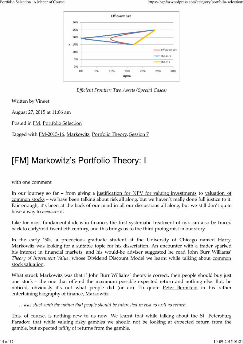
In general, depending on whether the value of the correlation is such that or , or, the efficient frontier changes as below:
Portfolio Selection | A Matter of Course https://pgpfm.wordpress.com/category/portfolio-selection/
13 of 17 10-09-2015 01:21
Efficient Frontier: Two Assets (Special Cases)
Written by Vineet
August 27, 2015 at 11:06 am
Posted in FM, Portfolio Selection
Tagged with FM‐2015‐16, Markowitz, Portfolio Theory, Session 7
with one comment
In our journey so far – from giving a justification for NPV for valuing investments to valuation ofcommon stocks – we have been talking about risk all along, but we haven’t really done full justice to it.Fair enough, it’s been at the back of our mind in all our discussions all along, but we still don’t quitehave a way to measure it.
Like for most fundamental ideas in finance, the first systematic treatment of risk can also be tracedback to early/mid‐twentieth century, and this brings us to the third protagonist in our story.
In the early ’50s, a precocious graduate student at the University of Chicago named HarryMarkowitz was looking for a suitable topic for his dissertation. An encounter with a trader sparkedhis interest in financial markets, and his would‐be adviser suggested he read John Burr Williams’Theory of Investment Value, whose Dividend Discount Model we learnt while talking about commonstock valuation.
What struck Markowitz was that if John Burr Williams’ theory is correct, then people should buy justone stock – the one that offered the maximum possible expected return and nothing else. But, henoticed, obviously it’s not what people did (or do). To quote Peter Bernstein in his ratherentertaining biography of finance, Markowtiz
…was stuck with the notion that people should be interested in risk as well as return.
This, of course, is nothing new to us now. We learnt that while talking about the St. PetersburgParadox: that while valuing risky gambles we should not be looking at expected return from thegamble, but expected utility of returns from the gamble.
Portfolio Selection | A Matter of Course https://pgpfm.wordpress.com/category/portfolio-selection/
14 of 17 10-09-2015 01:21
We’ve already talked at length about the implications of concavity of utility curves. One of theconsequences of that was for any risky gamble , expected utility is always less than the
utility of the payoff (mathematically also known as the Jensen’s inequality for concave
functions), i.e.:
Markowitz figured this out too, and he exploited this idea to come up with a way to quantify thetrade‐off between risk and return.
…
Given a certain starting wealth , Markowitz studied the change in expected utility to marginalinvestments in risky gambles.
That is, he considered the quantity for any small risky gamble relative to the
starting wealth .
As you may have done in your statistics courses, a useful way to think about a risky gamble is as arandom variable (something that takes a different value depending on the ‘state of the world’). Sincewe can talk about as a random variable, we can talk about its expected value, say , and variance,say .
With small we can evaluate as a Taylor series, and then the expected utility from
wealth including the gamble can be written as:
With small we can ignore the the exponents of greater than , and this gives us:
Given a certain (sure) starting , we can write the above as:
that is, the change in expected utility:
Given that is small, its expected value , being an average, would be smaller still and we canignore the higher powers of to give:
Since is known, so are , and we have:
where because concavity of implies and . The
Portfolio Selection | A Matter of Course https://pgpfm.wordpress.com/category/portfolio-selection/
15 of 17 10-09-2015 01:21
coefficient defines a measure of relative risk aversion. That is, higher the value of , morerisk‐averse the person, and lower its value more risk‐loving the person. (What would be the value of for a risk‐neutral person? What about for a risk‐loving person?)
That is, the change in expected utility from a marginal gamble depends only on the expected returnand variance of the gamble. And expected utility goes up as the expected return from the gambleincreases and goes down as variance increases.
For small gambles, then according to Markowitz people should only consider a single number to talkabout risk, i.e. its variance , irrespective of the number of states of the world. This turned out to be arevolutionary idea in the history of finance, and is a cornerstone in the theory of portfolio choice andasset pricing. For his efforts Markowitz was awarded the Nobel Prize in Economics in 1990.
This result, that however complex the world maybe, for small gambles people need only consider theexpected return and variance of the gamble will form the basis for our further discussions.
…
Not only did Markowitz notice that people care both about risk and return, he also observed thatpeople held not one but a portfolio of stocks. Just on its own, the fact that people should care aboutexpected return and variance of gambles doesn’t necessarily imply that people would hold multiplestocks. If they knew their degree of risk‐aversion, they would just want to pick one that offered the‘right’ trade‐off for them.
The fact that people could and did hold a portfolio of stocks made ample economic sense. Consider thefollowing two risky gambles:
It should be clear that by holding half of each and , an investor could make his end‐of‐periodpayoff the same (= 100), irrespective of the end‐of‐period state of the world, i.e. the portfolio of and with equal percentage invested in each is completely risk‐less.
This, of course, is an extreme example and in general such gambles would be rare that offered perfectlynegatively correlated payoffs. However, Markowitz’s point had been made. As long as end‐of‐periodpayoffs are not perfectly positively correlated investors could reduce the variance or risk associatedwith the end‐of‐period payoffs by holding multiple stocks. We’ll generalize this idea next.
Written by Vineet
August 27, 2015 at 11:02 am
Posted in FM, Portfolio Selection
Tagged with FM‐2015‐16, Markowitz, Portfolio Theory, Session 7
Portfolio Selection | A Matter of Course https://pgpfm.wordpress.com/category/portfolio-selection/
16 of 17 10-09-2015 01:21
Blog at WordPress.com. The Journalist v1.9 Theme.
Follow
Build a website with WordPress.com
Portfolio Selection | A Matter of Course https://pgpfm.wordpress.com/category/portfolio-selection/