Position control of a mobile robot

Position Control of a Mobile Robot

by

Pieter Winter

Position Control of a Mobile Robot

by

Pieter Winter

Thesis presented in partial fulfilment of the requirements for the degree of Master in

Electronic Engineering at the University of Stellenbosch.

Study leaders: Prof JB de Swardt

Declaration

I, the undersigned, hereby declare that the work contained in this thesis is my

own original work and has not previously in its entirety or in part been

submitted at any university for a degree.

______________ ______________

Signature Date

ABSTRACT

Position calculation of mobile objects has challenged engineers and designers for years

and is still continuing to do so. There are many solutions available today. Probably the

best known and most widely used outdoor system today is the Global Positioning System

(GPS). There are very little systems available for indoor use.

An absolute positioning system was developed for this thesis. It uses a combination of

ultrasonic and Radio Frequency (RF) communications to calculate a position fix in doors.

Radar techniques were used to ensure robustness and reliability even in noisy

environments. A small mobile robot was designed and built to test and illustrate the use

of the system.

OPSOMMING

Posisiebeheer van mobiele objekte is ’n probleem wat al vir baie jare vir ingenieurs ’n

uitdaging is. Menige oplossings is al gevind vir hierdie probleem. Die bekendste stelsel is

seker die Globale Posisionering Stelsel (GPS). Hierdie stelsel is slegs geskik vir

buitenshuise beheer. Daar is baie min stelsels beskikbaar vir binnenshuise posisiebeheer.

’n Absolute posisioneringstelsel is vir hierdie tesis ontwikkel. Dit gebruik ’n kombinasie

van ultrasoniese en Radio Frekwensie (RF) kommunikasie om ’n posisie-bepaling te

doen. Radar tegnieke is gebruik om te verseker dat die stelsel robuust is, selfs in ’n

raserige omgewing. ’n Klein mobiele robot (Peete5) is ontwerp en gebou om die stelsel

te toets en die gebruik daarvan te illustreer.

ACKNOWLEDGEMENTS

Special thanks to:

− Johan de Swardt

Gave me the opportunity to do this thesis and helped with advice, and hardware.

− Johan Gericke

Not only a colleague but also a study leader. Helped with advice and taught me a

lot about electronic and RF design.

− JC van der Walt

Gave advice with the Kalman filter and position control algorithms.

− John Hawkins

Helped with any problems encountered in Solid Works.

− Chrisna Winter

Endless support and patience.

TABLE OF CONTENTS

ABSTRACT iv

ACKNOWLEDGEMENTS vi

ABBREVIATIONS i

LIST OF FIGURES ii

LIST OF TABLES iv

Chapter 1 Introduction 1

1.1 Design goals 1

1.2 Position information and robots 1

1.2.1 Relative positioning 1

1.2.2 Absolute positioning 2

1.3 Position control in Peete5 3

1.4 Features of Peete5 3

1.5 Design process 5

1.6 Organization of chapters 7

Chapter 2 Mechanical positioning 8

2.1 Introduction 8

2.2 Calculating position 9

2.3 Calculating wheel travel 10

2.4 Implementation of calculating wheel travel 11

2.5 Non-idealities 12

2.5.1 Step counter resolution 12

2.5.2 Wheel radius and robot width 12

2.5.3 Wheel slip 13

2.6 Conclusion 14

Chapter 3 Ultrasonic / RF positioning 15

3.1 Introduction 15

3.2 Communication Network 16

3.2.1 Concept 16

3.2.2 Example 19

3.2.3 Data Packet format 21

3.2.4 Preamble 21

3.2.5 Sync word 21

3.2.6 Source Address 22

3.2.7 Destination Address 22

3.2.8 Data 22

3.2.9 CRC 22

3.2.10 Stop 22

3.2.11 Packet Protocol 22

3.2.12 Response message 24

3.2.13 Messages 25

3.2.14 Implementation 26

3.3 Position calculation 27

3.3.1 Position function 27

3.3.2 Simulation 31

3.4 Ultrasonic Positioning 35

3.4.1 Concept 35

3.4.2 Simple solution 36

3.4.3 Barker code 38

3.4.4 Simulation 41

3.4.5 Implementation 54

3.4.6 Distance Calibration 63

3.5 Conclusion 65

Chapter 4 Electronic Design 66

4.1 Introduction 66

4.2 PCB Block Diagram 67

4.3 Main CPU 69

4.3.1 Pulse Width Modulator 69

4.3.2 Analogue to Digital Converter 70

4.3.3 Serial Controller Interface 72

4.3.4 Serial Peripheral Interface 74

4.3.5 Controller Area Network 74

4.4 RX DSP 75

4.5 USB to UART converter 76

4.6 Power Supply 76

4.6.1 12V regulated voltage 77

4.6.2 5V regulated voltage 77

4.6.3 3.3V regulated voltage 77

4.7 Stepper Motor drivers 78

4.8 Ultrasonic transmit circuitry 79

4.9 Ultrasonic receive circuitry 84

4.10 RF Transceiver 84

4.11 Inclinometer 85

4.12 Gyro 86

4.13 Servo Motor 86

4.14 Video camera and video transmitter interface 87

4.15 Conclusion 87

Chapter 5 Software 89

5.1 Introduction 89

5.2 Delphi software 90

5.2.1 Module testing software 90

5.2.2 Pendulum simulation 92

5.2.3 Ultrasonic Simulation software 95

5.3 Matlab software 95

5.4 C software 95

5.4.1 Application Layer 97

5.4.2 Peripherals 97

5.4.3 Hardware Abstraction Layer 97

5.5 Conclusion 98

Chapter 6 Mechanical Design 100

6.1 Introduction 100

6.2 Design Goals 101

6.3 Peete5.0 102

6.3.1 Advantages 103

6.3.2 Disadvantages 104

6.4 Peete5.1 104



6.5 Peete5.2 107



6.6 Final solution 109



6.7 Conclusion 112

Chapter 7 Keeping Peete5 upright 113

7.1 Introduction 113

7.2 Sensor calibration 114

7.2.1 Inclinometer 114

7.2.2 Gyro 116

7.3 Kalman filter 117

7.4 Simulation 120

7.5 Conclusion 120

Chapter 8 Conclusion and suggestions 122

8.1 Conclusion 122

8.1.1 Position control 122

8.1.2 Electronic and software design 123

8.1.3 Mechanical Design 124

8.2 Suggestions 125

8.2.1 Simulation 125

8.2.2 Electronic design 125

8.2.3 Ultrasonic positioning 126

APPENDIX A : IIR filter implementation in Delphi and C 128

APPENDIX B : Communication messages 134

APPENDIX C : Schematics 148

APPENDIX D : Source code 155

APPENDIX E : Mechanical Drawings 159

INDEX 168

i

ABBREVIATIONS

APP Application Layer

CAN Controller Area Network

CPU Central Processing Unit

CRC Carrier Redundancy Check

DAC Digital to Analogue Converter

DSP Digital Signal Processor

FSK Frequency Shift Key

FIR Finite Impulse Response

GPS Global Positioning System

HAL Hardware Abstraction Layer

IC Integrated Circuit

IIR Infinite Impulse Response

MDI Multiple Document Interface

MIPS Million Instructions per Second

NAK Not Acknowledge

RAM Random Access Memory

ROM Read Only Memory

RC Resistor Capacitor

RF Radio Frequency

RSSI Received Signal Strength

RX Receiver

SCI Serial Controller Interface

SPI Serial Peripheral Interface

PCB Printed Circuit Board

SLIP Serial Line Internet Protocol

TX Transmitter

USB Universal Serial Bus

UART Usynchronous Asynchronous Receiver Transmitter

ii

LIST OF FIGURES

Number Page

Figure 2-1: Basic robot movement 9

Figure 3-1: Communication layers 18

Figure 3-2: Example of a message transaction 19

Figure 3-3: Data packet format 21

Figure 3-4: Message protocol flow diagram 23

Figure 3-5: 2D positioning with 2 beacons. 27

Figure 3-6: Distance measured from a beacon 30

Figure 3-7: Output of pos_calc_sim with 3 reference beacons 32

Figure 3-8: Output of pos_calc_sim with 6 reference beacons 32

Figure 3-9: Position calculation with three beacons. 33

Figure 3-10: Dependence of position error on beacon placement 34

Figure 3-11: Position calculation with four beacons. 34

Figure 3-12: Simplified range finding system 35

Figure 3-13: Simple ultrasonic measurements 37

Figure 3-14: Autocorrelation of different length random streams 39

Figure 3-15: 13-bit Barker code autocorrelation 41

Figure 3-16: Complete ultrasonic system 42

Figure 3-17: Generated TX code 43

Figure 3-18: Modulated TX signal 44

Figure 3-19: Spectrum of modulated TX signal 45

Figure 3-20: Ultrasonic pulse and its spectrum 46

Figure 3-21: Generated TX signal 47

Figure 3-22: Output after first correlation 48

Figure 3-23: FIR filter response 49

Figure 3-24: Second correlation output 50

Figure 3-25: Output of simulation program with no noise 51

Figure 3-26: Output of simulation program with noise 52

Figure 3-27: Output of simulation program with clock error of 400 Hz 53

Figure 3-28: Flow diagram for generating the modulated TX code 57

Figure 3-29: Flow diagram for demodulating the received signal 60

iii

Figure 3-30: Correlation peak counter over distance 64

Figure 4-1: Motherboard block diagram 67

Figure 4-2: Complimentary pair PWM with dead time 69

Figure 4-3: Equivalent circuit for ADC loading 71

Figure 4-4: Double buffering for SCI TX 73

Figure 4-5: Ultrasonic transmitter block diagram 80

Figure 4-6: Simple Model of an ultrasonic transducer 81

Figure 4-7: Circuit diagram of ultrasonic transmitter 81

Figure 4-8: SPICE simulation output of ultrasonic transmitter 83

Figure 4-9: Servo motor control signal 86

Figure 5-1: Screen capture of module_testing 91

Figure 5-2: Forces simulated in pendulum simulation 93

Figure 5-3: Screen capture of pendulum simulation 94

Figure 5-4: Partitioning of C software 96

Figure 6-1: Mechanical drawing of Peete5.0 102

Figure 6-2: Peete5.0 motor assembly 103


Figure 6-4: Servo bracket – Unfolded 106

Figure 6-5: Servo bracket - Folded 106


Figure 6-7: Mechanical drawing of final design 109

Figure 6-8: View of Peete5 without front panel 111

Figure 6-9: Photograph of Peete5 112

Figure 7-1: RAW ADC values for inclinometer calibration 115

Figure 7-2: Measuring g with an inclinometer 115

Figure 7-3: Estimating gyro drift 120

iv

LIST OF TABLES

Number Page

Table 3-1: Peete5 communication command messages 26

Table 3-2: Explanation of second correlation assembler code 62

Table 7-1: Calculating inclinometer offset and scale factor 116

Table 8-1: Board states 135

Table 8-2: Warning bits 135

Table 8-3: Warning bits 135

1

Chapter 1 Introduction

1.1 Design goals

Peete5 is the name of the small robot developed for this

thesis. The design goals of this thesis were to design a

remote controlled mobile robot with an absolute

position control system for indoor use.

1.2 Position information and

robots

Position control has long been a problem for many

designers. Robots (especially autonomous robots) need

to know where they are.

The paper “Where am I” [3] states: “Perhaps the most

important result from surveying the vast body of literature on mobile robot positioning is

that to date there is no truly elegant solution for the problem”. This thesis will attempt

to develop an elegant solution to this problem.

There are two types of position measurements:

• Relative positioning and

• Absolute positioning.

Types of relative positioning used are Odometry and Inertial Navigation while

absolute positioning methods available are Active beacons, Artificial landmark

recognition, Natural landmark recognition and Model Matching.

1.2.1 Relative positioning

Odometry uses wheel position (like wheel encoders, stepper motors etc.) to calculate the

distance travelled by the robot as well as the angle in which the robot is travelling. The

advantage of this system is that it can be completely self contained.

5

Peete


2

1

Inertial Navigation uses inertial sensors like gyroscopes and accelerometers to measure

the speed and acceleration of the robot in its axes of movement. The speed and

acceleration information can be used to calculate the robots position. This is also a

method self contained positioning.

The main disadvantage of Odometry and Inertial Navigation is that no reference

position is used. This is a problem because of small errors that may accumulate over

time. A very accurate and expensive gyroscope may have a rate offset error of 1×10-3

deg/sec. This may sound very small but if it is integrated over an hour, then the robot

would think that it has turned by 3.6 degrees. If it travels only 1 meter, then it will have

made a 6 cm position error!

Relative positioning can be improved quite substantially if the robot could have some

kind of reference to compare to. If the gyro error could be calculated, then the robot

could use the accurate gyro data for short distance navigation and some sort of coarse

reference to keep it on track.

1.2.2 Absolute positioning

Absolute positioning is normally less accurate than relative positioning but it has the

advantage that the magnitude of the errors stays the same where as the magnitude of

error could grow unchecked with relative positioning.

Active beacons use beacons at known locations to calculate the position of the robot.

The best known and most advanced example of active beacon position calculation

today is the Global Positioning System (GPS). A GPS receiver would measure the

distance to four ore more satellites orbiting the earth at known positions. The satellite

position information together with the distance measurement can be used to calculate the

position of the GPS receiver with an error as small as 1 meter!

5

Peete


3

1

Artificial Landmark recognition is used where artificial shapes or objects are used to

calculate the position of the robot. One such example would be to paint a grid on the

floor. A robot would be able to count the squares that it is moving over to calculate its

position.

Artificial Landmark recognition requires that the environment be prepared prior to

unleashing the robots in it. This may not always be possible or practical. Natural

Landmark recognition can be used in such cases. Unmanned Aerial Vehicles (UAV)

may look at mountain ranges to make rough position estimations.

Model Matching uses the robots on board sensors to compare its environment to a

pre-stored map. If a robot is placed in a room and it could measure the distance to all

four walls, then it could calculate its position if the dimensions of the room was known.

1.3 Position control in Peete5

Peete5 will attempt to add a new method of position control to the long list of position

methods currently available to robot designers. It will investigate the use of a relative

positioning system by using stepper motors to calculate its position. It will also develop

an absolute positioning system that uses a combination of ultrasonic and Radio

Frequency (RF) communications.

The position system developed for Peete5 is aimed at short range interior position

control. The aim is to develop and demonstrate a positioning system capable of

calculating the absolute position of the robot with accuracy in the order of millimetres.

1.4 Features of Peete5

This robot is a small (stands about 200mm tall), two-wheeled robot that can accurately

calculate its own position by using a network of ultrasonic reference transmitters. Radar

5

Peete


4

1 techniques like special signal encoding are used to calculate the distance to reference

beacons. This information is then used to calculate the robots position.

The position calculation is done in a similar manner to GPS system. A 13-bit barker

code is transmitted from a reference board. This code is modulated on the 40 kHz

ultrasonic frequency. Two high speed correlators (both running at 160 k samples per

second) correlate the received signal and run a peak detection algorithm. The time when

the peak is detected, relative to a timing reference transmitted via a radio link, is used to

calculate the range to the transmitter. The range information from several beacons is

then used to calculate the position of the robot.

It can be controlled from a PC via and RF-link. It is equipped with a video camera and

video transmitter that enables the remote user to see what the robot is seeing.

Features:

• Two high-speed, 60MIPS DSP’s, connected with a high speed CAN bus (data

processing of 120MIPS).

• Complex demodulating algorithms that enables the robot to know exactly where

it is (when in view of 3 or more reference transmitters).

• 19200 baud rate, half duplex 433MHz RF link.

• USB interface to a PC/laptop.

• High resolution BW camera with 2.5 GHz video transmitter.

• Two stepper motors with a control resolution of 56.25µ degrees and a maximum

speed of 1000degrees/second.

• Stepper motor current under software control for current between 0 A and 1.2 A.

• Small, light-weight Lithium Ion battery pack for 18 V, 2 Ah operation.

• Servo motor for position control of the camera head (up-down movement) in 0.5

degree steps.

5

Peete


5

1 • Highly accurate, low noise, micro-machined inclinometer and gyroscope

reference sensors.

• Switch-mode power supply for input voltages between 12 V and 20 V.

• 20V, fast switching push-pull configuration used for ultrasonic transmitter.

• Sensitive 40 kHz ultrasonic receiver.

• Highly flexible and robust communication network that enables any device in the

network to talk to any other device.

• User-friendly real time debugging software has been developed for debugging

and programming of any device in the RF network.

• Solid, robust and simple mechanical design.

1.5 Design process

The goal of this thesis was not only to develop an accurate positioning system but to also

develop a highly flexible and easy to use feature packed robot (Peete5). Ease of use and

robustness was high on the priority list when designing Peete5. The following steps

summarize the process followed when developing Peete5:

1. Ultrasonic range finding was selected as the method for position calculation.

The reason for this is that the slow speed of sound implies long propagation

delay of the ultrasonic pulses. Ultrasonic range finding is a commonly used

method for measuring distance between objects. It is widely used in motor cars

today to measure the clearance in front of and behind the car.

2. The ultrasonic transducer was investigated and modelled.

A model of an ultrasonic transducer was developed to understand how it works.

The model was simulated in SPICE to confirm the workings of the transducer.

3. Development of an ultrasonic transducer driver.

When the model of the ultrasonic circuit was understood, a circuit was developed

to optimally drive the ultrasonic transducer.

5

Peete


6

1 4. First PCB was developed.

A PCB was developed that used a DSP56F801 Digital Signal Processor for both

transmitting and receiving. This PCB had a 5 V input voltage and generated 20 V

(needed to drive the ultrasonic transducer) with a switch mode regulator. It used

a complex buffering system for communications over the RF link.

The 20V switch mode regulator design never worked and the buffering system

for the communications was unreliable and difficult to handle in the software. A

modification was done on the board to eliminate the buffering. A normal UART

interface was implemented where the TX/RX operation of the RF transceiver

was controlled in the software driver layer of the SCI interface on the DSP. This

design was also used in the final solution.

The ultrasonic driving circuitry was tested with the use of an external power

supply. The receiver algorithm could never be tested on the DSP56F801 because

it did not have enough RAM to implement the correlation needed. Although the

processor had 1 kWords of RAM, and only 700 Words of RAM was needed, it

could not implement a circular buffer because the compiler uses the RAM

starting at address 0. This was overlooked when the processor was chosen.

The modification on the RF transceiver meant that an external SCI port for

debugging was no longer available. This made debugging of the hardware and

software very difficult.

5. A block diagram was drawn up to state the requirements of a single PCB that

could be used for ultrasonic transmitting as well as all the circuitry needed to

control the robot. This included motor drivers, RF transceiver etc.

6. The components for the final PCB were selected based on the specifications

from the block diagram.

7. Simple test routines were written to ensure that the RX processor would have

enough RAM for the computational tasks.

5

Peete


7

1 8. A schematic library was created that contained all of the components that would

be used on the Peete5 motherboard. This library included both the schematic

symbol of the component as well as its PCB footprint.

9. The schematic diagram was drawn up and from there the PCB was developed.

10. The PCB was made as small as possible in order to simplify the mechanical

design. The components on the PCB were placed in groups in such a way that

shielding could be provided for the RF circuitry. The sensitive analogue circuitry

was kept separate from noisy components like the switch mode power supply

and stepper motor drivers.

11. PC test software as well as the embedded application software was developed.

12. Once the functionality of the electronic hardware was verified, the mechanical

design was done. The parts for the mechanical components were made and the

robot could be assembled.

13. The system was integrated to get to the completed Peete5 robot.

1.6 Organization of chapters

This document is divided in to 8 chapters. Chapters 2 & 3 will demonstrate two

different methods of position control: absolute and relative.

The next three chapters (chapters 3 to 6) will explain the design of hardware and

software that supported the position control systems.

The final chapter (chapter 7) expands on the control algorithms used to keep the robot

upright. This was not one of the original design considerations of this project.

Chapter 2 Mechanical positioning

2.1 Introduction

Two stepper motors control Peete5’s motion.

The control software is capable of accurately

controlling the speed of the motors as well as

keeping track of the precise motion of the

wheel. If no wheel slip occurred, and the

dimensions of the robot could be very

accurately measured, then the robot’s position

could be calculated based on the wheel motion

alone. This is a relative form of position control. The robot will start off at a know

position and calculate its position relative to the original starting position.

This chapter will show how the wheel motion can be used to calculate the robot’s

position but also explain why this information cannot be used as a stand-alone solution.

This chapter will start by showing how wheel motion can be used to calculate the robot’s

position. It will then show how the stepper motors were used to calculate the wheel

motion. The chapter ends off by pointing out the problems in relative position control

systems.

5

Peete


9

2

2.2 Calculating position

Figure 2-1 shows some basic forms of robot movement. The dotted line is the robot’s

initial position while the bolder line is the final position after some time, ∆t. The change

in position, ∆x and ∆y, can be used to calculate the robot’s final position (x,y).

θ

Dr

W/2

W

(x,y)(x,y) θ

Dr

Dl

(x,y)

DrDl

a b c a) One wheel standing still while the other is moving. b) Both wheels turn the same amount but in opposite directions. c)

Both wheels turn the same amount in the same direction.

Figure 2-1: Basic robot movement

The following equations satisfy all three basic robot movements given in Figure 2-1:

WDD rl −

=θ

2-1

2rl DDD +

=

2-2

)sin()cos(

θθ

DyDx

=∆=∆

2-3

5

Peete


10

2

Where:

Dl and Dr are the distances travelled by the left, and the right wheels respectively.

W is the width of the robot, measured as the distance between the centres of the

two wheels.

θ is the direction faced by the robot.

Based on the equations shown, the robot’s position can be calculated given the

movement of the two wheels.

2.3 Calculating wheel travel

The equations derived in section 2.2 had three inputs: Dl, Dr and W. W (the width of

the robot) can be measured manually. Dl and Dr need to be calculated from the

movement of the stepper motors.

The two stepper motors have a step size of 1.8°/step. This means that the wheel will

turn by 1.8° for every step. The driver used for controlling the stepper motor also allows

micro stepping where each stepper motor step can be divided in to 32 micro-steps. The

number of micro-steps is determined by the resolution of the DAC (Digital to Analogue

Converter) of the stepper motor controller. In this case a 6-bit DAC is used, resulting in

32 micro steps per step (the MSB of the DAC is used as the sign bit). This now means

that for every micro step, the wheel will turn by 0.05625°.

The stepper motor control software maintains a signed 32-bit counter for each of the

two motors. Every time a positive step is executed, the counter is increased by 1 and

decreased by 1 every time that a negative step is executed. These counters can therefore

be used to determine the orientation of the wheel.

For example, if the wheel turns by 90°, the counter will increment by:

5

Peete


11

2

stepsstep

1600/5626.0

90=

o

o

To calculate the distance that the wheel travelled, the following equation can be used:

β×= RDwheel

2-4

Where:

Dwheel is the distance travelled by the wheel.

R is the radius of the wheel.

β is the rotation of the wheel (in radians).

If the radius of the wheel (R) is 40mm and the number of micro steps counted is 1600,

then the distance travelled by the wheel (Dwheel) is:

mmstepstepsmmDwheel 83.62)180/05625.01600(40 =×××= πo

2.4 Implementation of calculating wheel travel

The function “calc_position” was written to calculate the robot’s position given only the

movement of the wheels. This function stores the previous stepper motor counter

values and then gets the difference between the stored and current value each time the

function is called.

The “calc_position” function is called periodically to calculate the robot’s position. The

source code for “calc_position” can be found in 1 in APPENDIX D. It will calculate

the straight-line movement between the previous position and the current position. The

position calculation will increase in accuracy if the function is called more frequently.

5

Peete


12

2

2.5 Non-idealities

There are a number of non-idealities that limit the accuracy of the mechanical position

control. The most important ones are:

1. Wheel slip.

2. Wheel radius and robot width.

3. Step counter resolution.

2.5.1 Step counter resolution

One pitfall in this method of position control is the wrapping of the counters. The step

counters that count the micro steps have a limited size of 32-bits. This means that it will

wrap at 231-1 and –231. This wrapping must be taken in to account when the difference is

calculated. These digital limitations are often overlooked and cause havoc that is often

just regarded as “spurious” behaviour.

In the case of a counter that can count 231-1 micro steps before wrapping, the robot can

cover a distance of 2.147 billion micro steps before wrapping occurs. From equation 2.3

this means that the robot will travel 84km before wrapping occurs. This is so infrequent

that one may be tempted to ignore it all together. This may be the case for Peete5 that is

only switched on for a short while but these types of problems have to be understood.

The problem may have been significant if an 8-bit microprocessor was used for example.

Only four lines of code were used to solve this problem.

2.5.2 Wheel radius and robot width

Errors when measuring the width of the robot (distance measured between the centres of

the two wheels) and the wheel radius are big causes of inaccuracy. The percentage error

on the wheel radius, for example, directly equates to a percentage error in wheel travel

and thus robot position. The same applies to the robot width.

5

Peete


13

2

These two values were accurately measured as follows:

Wheel radius:

1. The wheel radius was measured with a calliper to get a reasonably accurate

starting value. The wheel radius was measured to be 42mm.

2. The measured value was taken and the code was implemented for position

control. The robot was then commanded to move forward at a constant speed.

3. After the robot had travelled a distance of about 3 meters, it was commanded to

stop. A tape measure was used to measure the distance that the robot has

travelled and the calculated value was read back from the robot itself. The error

between the measured and calculated value was then fed back in to the original

wheel radius to get a more accurate measurement.

4. The final value of the wheel radius was determined to be 40.90841584mm. With

this value an error of only 3mm accumulated over a distance of about 3 meters.

Robot width:

1. A calliper was used to get a starting value.

2. The robot was turned through 3600° and then the calculated angle was read from

the robot. The error was fed back to the width to get a more accurate width.

3. The final value of the width was 206.38361620mm.

2.5.3 Wheel slip

Wheel slip makes a large contribution to error in mechanical position calculation. If the

robot is moving only forward and backwards on a non-slippery surface then wheel slip is

not an issue and accurate position information is obtained. Wheels with a non-zero

width imply slip when the robot turns and will cause position inaccuracies.

Consider Figure 2-1 (a). In this figure the robot turns around one wheel only, i.e. the one

wheel is standing still while the other is turning. The angle of rotation is calculated by

using the distance between the two wheels (in this figure the wheels do have a zero

5

Peete


14

2

width). The problem is that the stationary wheel will not turn exactly on its centre. Due

to the surface of the wheel and the surface that it is turning on, the centre of rotation will

move. It is impossible to keep track of the rotation angle when this happens. The same

problem will occur not only when the robot is stationary, but whenever it is turning,

where one wheel is turning at a different speed to the other.

2.6 Conclusion

Mechanical positioning can be implemented very accurately. Take modern day ink-jet

printers for example. They can accurately control the x-y location of a dot of ink on an

A4 page to about 1/1200dpi = 21µm! The printer also uses stepper motors to control

the position. The difference however is that the printer controls x and y position

separately and that very careful measures are taken to ensure no slip.

Although wheel radius and robot width can be accurately determined, a 1% error can

quickly accumulate because no reference is available to zero the accumulated error. The

wheel slip is the final nail in the coffin. Gyros could be used to counter wheel slip but

they too have drift that must be taken out. All-in-all mechanical position control for a

robot is not a very good idea. It must not be totally discarded though. The mechanical

position can be used to compensate for sensor drift and inaccuracy. A good position

calculation solution may be found by combining it with other methods. An absolute

method of position control is explained in the next chapter.

Chapter 3 Ultrasonic / RF positioning

3.1 Introduction

Peete5 can be placed at a random location in a room

and when it is switched on, it will know to within

about 8 cm exactly where it is. This means that it

may navigate the room by using a mental map of the

room. Peete5 can do this because it is equipped with

a sophisticated positioning system that uses both a

RF communication link as well as ultrasonic range

finding system. This chapter will explain how these

two systems are used together to get an accurate

position fix on the robot.

This chapter is divided in to three main parts. The first part will explain the

communication network used for communications between the different units. This

network is the backbone of the positioning process. It is also used for debugging

communications from a PC to any one of the boards in the system.

The second part develops the position calculation function. This is the function that

Peete5 uses after gathering all the required sensory information. The matrix maths is

explained and the final solution of the function is demonstrated. It will also show how

the function was simulated on a PC to prove that it works correctly.

The third part explains how the ultrasonic range finding system works. The range

information is the actual measurement that is used to calculate the robot’s position. The

PC simulation software is demonstrated and the final implementation in the DSP is

explained.

5Peete


16

3

3.2 Communication Network

3.2.1 Concept

The communication network used for communication on Peete5 is simple, reliable and

very flexible network of communications that allow any device in the network to talk to

any other device in the network. There are a number of hardware layers that are used for

communication. All these layers must be understood and the flow of data over these

layers is crucial. The five hardware links used in Peete5 is:

• USB

The Universal Serial Bus (USB) is mainly used for debugging and remote control

of the robot. The communication over the USB bus will always be between a PC

and main motherboard CPU. The data on the USB bus goes through a USB to

SCI (Serial Communication Interface) converter. The SCI signal is native to the

CPU used and can be taken directly in to the CPU for communication.

• SCI

The SCI (Serial Controller Interface) is one of the on-board peripherals on the

CPU’s used. The physical hardware is set up and controlled by low level driver

software that was developed for the CPU. SCI is used for communications

between a PC and the CPU and for communications from one CPU to another

over an RF link.

• SPI

The SPI (Serial Peripheral Interface) is widely used for inter-device

communication. In Peete5 this interface is not part of the main communication

layer. The RF IC used has two interfaces. It uses SPI to control its registers (that

ultimately controls the functionality of the IC), and SCI for the actual RF

communications.

• CAN

CAN (Controller Area Network) is a high speed, high reliability network interface

that was developed for high reliability communication between multiple devices

on the same network. In Peete5 CAN is used for communication between the

main control CPU, and the RX CPU that is used for demodulating the received

5Peete


17

3

ultrasonic signal. CAN lend itself to multiple communication layers over the

same physical interface. In Peete5 this has been used to great advantage. Two of

the ports on the CAN bus has been used for a transparent communication layer.

This communication layer will work the same as the normal communication

layer. Two other ports have been used to quickly flag the start of, and end of an

ultrasonic transaction.

• RF

A 433MHz, FSK RF link is used for the RF communications. This is a half-

duplex link. The low-level driver software controls transmit and receive state on

the RF link. It does this by monitoring RSSI as well as transmitter and receiver

interrupts in the CPU hardware.

Because of the interaction between so many modules in the system, there must be an

easy communication flow of data from one module to another. A special protocol layer

has been developed in such a way that one module can talk to another module without

knowing the path that the data took or the physical hardware medium that was used for

the data transaction. This makes development and implementation much easier and

quicker.

5Peete


18

3

Application layer

Protocol layer

Comms layer

Hardware layer

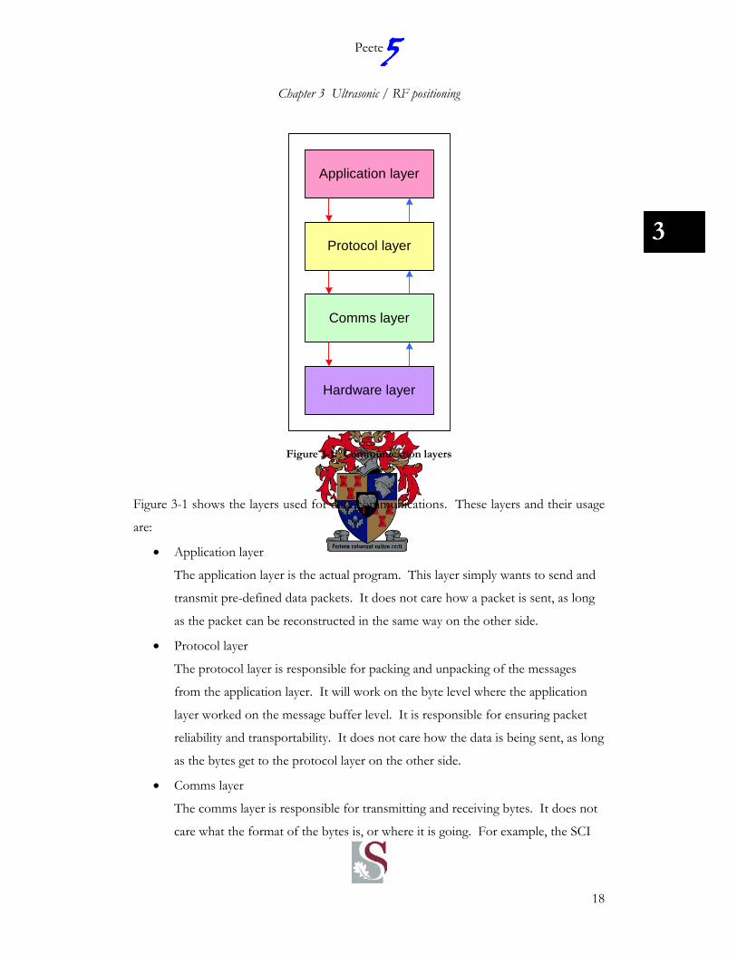
Figure 3-1: Communication layers

Figure 3-1 shows the layers used for data communications. These layers and their usage

are:

• Application layer

The application layer is the actual program. This layer simply wants to send and

transmit pre-defined data packets. It does not care how a packet is sent, as long

as the packet can be reconstructed in the same way on the other side.

• Protocol layer

The protocol layer is responsible for packing and unpacking of the messages

from the application layer. It will work on the byte level where the application

layer worked on the message buffer level. It is responsible for ensuring packet

reliability and transportability. It does not care how the data is being sent, as long

as the bytes get to the protocol layer on the other side.

• Comms layer

The comms layer is responsible for transmitting and receiving bytes. It does not

care what the format of the bytes is, or where it is going. For example, the SCI

5Peete


19

3

comms layer may receive a burst of bytes when a message is being transmitted or

received. Because of physical constraints (the bytes can only be sent over the bus

at a certain baud rate), it will buffer the bytes and monitor the activity on the bus

to send/receive the next byte when it becomes available. The different comms

layers were described at the start of this section.

• Hardware layer

The hardware layer is the physical transport layer. This layer works on the bit

level. It is sending and receiving single bits at a time. It may be a wire (CAN,

SCI, USB) with specific voltage levels, or it may be a RF carrier wave.

Each layer and its interfaces are very clearly defined. This is what made it possible to

have transparent data communications across the different hardware interfaces. Any one

of the layers below the application layer can be changed without affecting the basic

communication routines.

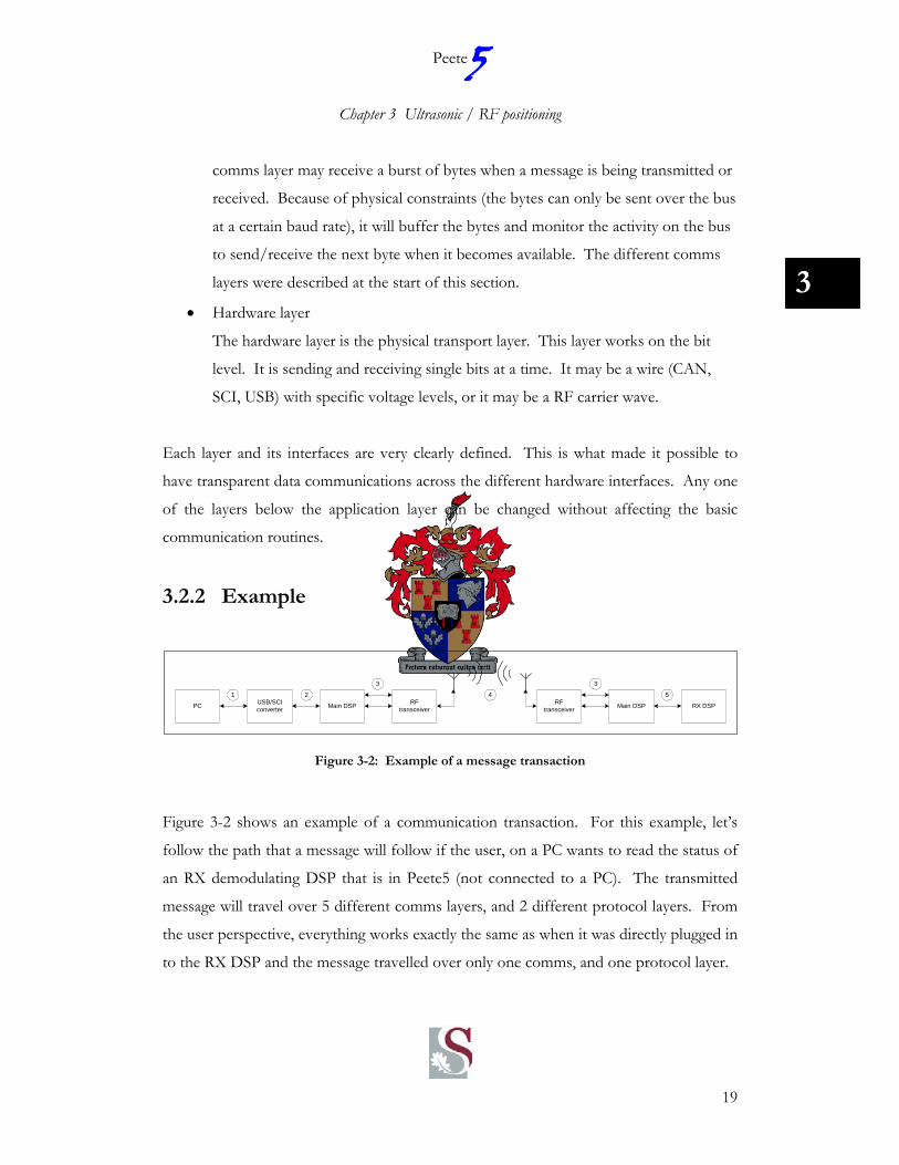
3.2.2 Example

PC USB/SCIconverter Main DSP RF

transceiverRF

transceiver Main DSP RX DSP

1 2

3

4

3

5

Figure 3-2: Example of a message transaction

Figure 3-2 shows an example of a communication transaction. For this example, let’s

follow the path that a message will follow if the user, on a PC wants to read the status of

an RX demodulating DSP that is in Peete5 (not connected to a PC). The transmitted

message will travel over 5 different comms layers, and 2 different protocol layers. From

the user perspective, everything works exactly the same as when it was directly plugged in

to the RX DSP and the message travelled over only one comms, and one protocol layer.

5Peete


20

3

Step 1: The PC will build up the packet to be transmitted (the data packet format can be

found in 3.2.3). The PC software will break up the packet in to a normal SLIP (Serial

Line Internet Protocol) packet and use the PC’s USB driver to transmit the data. The

data will travel over a screened, twisted pair USB cable.

Step 2: The USB to SCI converter will convert the USB data to a SCI data stream.

(Note: The USB link has its own protocol layer built in). The SCI data then travels on a PCB

track, at 3.3V voltage levels.

Step 3: The main DSP will receive the SCI bits and an interrupt will be generated when

a correct byte has been received. The comms layer will buffer these bytes for later

retrieval by the protocol layer. The protocol layer will periodically read in data buffers

and attempt to reconstruct a complete message. It will flag the application layer when

the message has been reconstructed, and pass the reconstructed message to the

application layer.

Step 4: The application layer would have determined that this message was not

addressed for it (remember that it is addressed to the RX DSP), and will transmit it over

the RF link. It will use both the SPI interface (to control the RF device IC) and the SCI

interface to transmit the packet over the RF link. It will also now use a different

protocol layer. The normal SLIP protocol cannot be used on the RF link because of

certain data constraints. The RF-SLIP protocol is now used.

Step 5: This is the same as step 4 but in this case the DSP is receiving data over the RF

link. The packet will be reconstructed and presented to the application layer. The

application will recognize that the packet is not addressed to it, and will forward the

packet on the CAN bus.

Step 6: The protocol layer on the RX board will receive the bytes from the CAN

comms layer, and attempt to build up the received packet. Once a complete packet is

received, it will be presented to the application layer. In this case, the application layer

will respond to the message since it is addressed to it. It will build up a packet to indicate

its status, and transmit it back on the comms layer that it was received on. From there

on, the whole process works again in reverse until the response is received by the PC,

and is displayed for the user.

5Peete


21

3

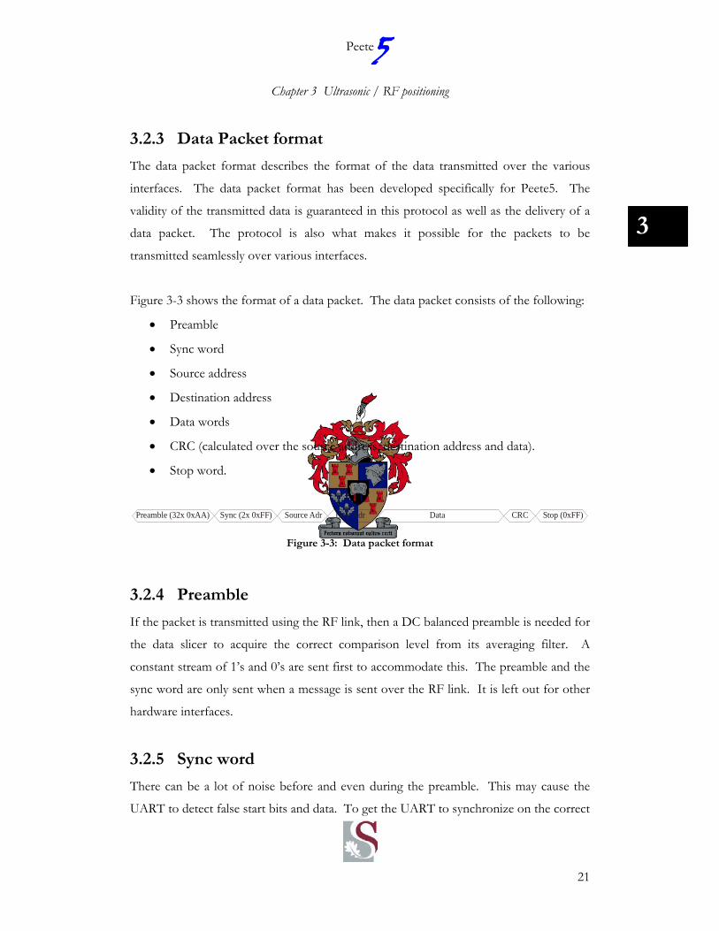
3.2.3 Data Packet format

The data packet format describes the format of the data transmitted over the various

interfaces. The data packet format has been developed specifically for Peete5. The

validity of the transmitted data is guaranteed in this protocol as well as the delivery of a

data packet. The protocol is also what makes it possible for the packets to be

transmitted seamlessly over various interfaces.

Figure 3-3 shows the format of a data packet. The data packet consists of the following:

• Preamble

• Sync word

• Source address

• Destination address

• Data words

• CRC (calculated over the source address, destination address and data).

• Stop word.

Preamble (32x 0xAA) Sync (2x 0xFF) Source Adr Dest Adr Data CRC Stop (0xFF)

Figure 3-3: Data packet format

3.2.4 Preamble

If the packet is transmitted using the RF link, then a DC balanced preamble is needed for

the data slicer to acquire the correct comparison level from its averaging filter. A

constant stream of 1’s and 0’s are sent first to accommodate this. The preamble and the

sync word are only sent when a message is sent over the RF link. It is left out for other

hardware interfaces.

3.2.5 Sync word

There can be a lot of noise before and even during the preamble. This may cause the

UART to detect false start bits and data. To get the UART to synchronize on the correct

5Peete


22

3

start bit in the data stream, 16 bits of 1 are sent. This means that the data stream will be

high, with only the stop bit. The UART should have synchronized after the first synch

word.

3.2.6 Source Address

The source address shows the origin of the data packet. This will be the ID of the

specific board that sent this packet. It is an 8-bit wide, unsigned byte.

3.2.7 Destination Address

Every packet has a destination. This is the ID of the board that the packet was intended

for. It is an 8-bit wide, unsigned byte. The following are globally used addresses and

should not be used by individual boards:

• 0x00 – Addressed to all.

3.2.8 Data

This block contains the data information to be sent and can be of any length as long as

the receiving device has enough memory to store the complete packet.

3.2.9 CRC

Every message is protected with a Carrier Redundancy Check (CRC). The CRC is

calculated over the source address to the last byte of data. It is a 16-bit wide, unsigned

word.

3.2.10 Stop

The stop byte signals the end of a message packet.

3.2.11 Packet Protocol

All the data is sent and received using a specific protocol. The following bytes are used

in the transmission protocol and may not be part of the data packet or the address bytes:

5Peete


23

3

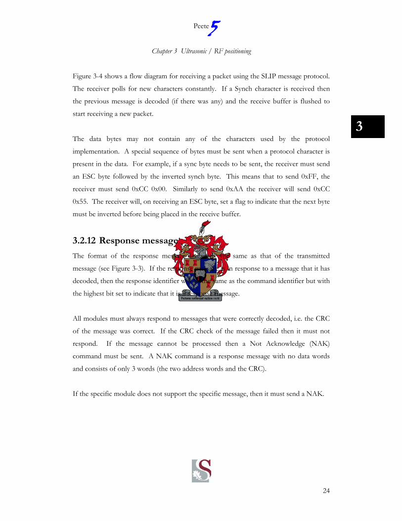
• 0xAA – This byte is used for the preamble.

• 0xFF – This byte is used to synchronize the UART and is used to signal the start

and end of a packet.

• 0xCC – This byte is used if any of the other protocol specific bytes are part of the

normal data packet. It is called the ESC byte.

Receive newcharacter

Is it Synch byte?

Put byte in receive buffer.

Is it ESC byte?

Is receive bufferfull?

Flush receive buffer

Wait for byte.

Y

N

N

N

Set ESC flag.

Is ESC flag set?

N

Invert byte and put inreceive buffer.

Clear ESC flag.Y

Is receivebuffer > 3 *

Flush Receive buffer.

N

Y

Calculate packet CRC.

Does CRC checkout OK?

N

Parse packet

Y

* The smallest possible packet size is 3 bytes.

Figure 3-4: Message protocol flow diagram

5Peete


24

3

Figure 3-4 shows a flow diagram for receiving a packet using the SLIP message protocol.

The receiver polls for new characters constantly. If a Synch character is received then

the previous message is decoded (if there was any) and the receive buffer is flushed to

start receiving a new packet.

The data bytes may not contain any of the characters used by the protocol

implementation. A special sequence of bytes must be sent when a protocol character is

present in the data. For example, if a sync byte needs to be sent, the receiver must send

an ESC byte followed by the inverted synch byte. This means that to send 0xFF, the

receiver must send 0xCC 0x00. Similarly to send 0xAA the receiver will send 0xCC

0x55. The receiver will, on receiving an ESC byte, set a flag to indicate that the next byte

must be inverted before being placed in the receive buffer.

3.2.12 Response message

The format of the response message is exactly the same as that of the transmitted

message (see Figure 3-3). If the response message is in response to a message that it has

decoded, then the response identifier will be the same as the command identifier but with

the highest bit set to indicate that it is a response message.

All modules must always respond to messages that were correctly decoded, i.e. the CRC

of the message was correct. If the CRC check of the message failed then it must not

respond. If the message cannot be processed then a Not Acknowledge (NAK)

command must be sent. A NAK command is a response message with no data words

and consists of only 3 words (the two address words and the CRC).

If the specific module does not support the specific message, then it must send a NAK.

5Peete


25

3

3.2.13 Messages

Table 3-1 lists all the supported messages within the modules used in Peete5. This table

lists all the command identifiers. Remember that the highest bit of the identifier will be

set if it is a response message.

Supported by: Description Command

identifier RX1 TX2 Main3

status

0x01

enter_sw_download 0x02

start_sw_download 0x03

program_flash 0x04

stop_sw_download 0x05

get_raw_adc 0x06

send_dist_pulse 0x07

force_calculate_distance 0x08

reset 0x09

set_motor_speed 0x0A

set_motor_current 0x0B

set_servo_angle 0x0C

get_last_dist_ 0x0D

get_mec_pos 0x0E

get_sensor_data 0x0F

Peek 0x10

new_beacon 0x11

update_position 0x12

get_beacon_info 0x13

1 Receiver processor (MC56F8322). 2 Transmitter board (MC56F8346). 3 Main Robot processor (MC56F8346).

5Peete


26

3

get_usonic_pos 0x14

Table 3-1: Peete5 communication command messages

The contents of the messages can be found in APPENDIX B.

3.2.14 Implementation

It should be clear by now that the implementation of the communication network

requires various hardware interfaces, as well as different layers of software. To discuss all

of this in detail is beyond the scope of this document. It will require an in depth

explanation of the different hardware layers, assembler code knowledge, etc. Instead, the

references for the different hardware layers, (CAN, SCI, SPI, USB and RF) can be used

together with the comments in the source code to better understand the lower two levels

of the communication network. See [5], [6], [7], [8] and [9].

5Peete


27

3

3.3 Position calculation

3.3.1 Position function

Figure 3-5 shows a two-dimensional (2D) surface with two beacons. The positions of

two beacons, B1 and B2 are known as (xB1,yB2) and (xB2,yB2) respectively. The robot will

measure the distance (r1 and r2) to the two beacons. If the robot measures the distance to

B1, it knows that it is somewhere on the rim of the smaller, blue circle. Measuring the

distance to B2 tells it that it is somewhere on the rim of the larger, red circle. The robots

absolute position is thus given where these two circles intersect.

x

y

R =(x ,y )1 1 1

B =(x ,y )1 B1 B1

B =(x ,y )2 B2 B2

R =(x ,y )2 2 2

Figure 3-5: 2D positioning with 2 beacons.

5Peete


28

3

The basic equation used to calculate the position of the robot is given by the equation of

a point on a circle:

( ) 222 ryx =+

3-1

To calculate the position of the robot in Figure 3-5, the robots position (x,y) must satisfy

both of the following equations:

( ) ( ) 21

21

21 BBB ryyxx =−+−

3-2

( ) ( ) 22

22

22 BBB ryyxx =−+−

3-3

Where rB1 and rB2 are the distance measured by the robot from beacon 1 and beacon 2

respectively. This results in two equations with two unknowns. Simultaneously solving

these two equations will give the two points shown in Figure 3-5 as R1 and R2.

One more beacon is necessary to resolve the ambiguity between R1 and R2. Write the

equation of the distance from the beacon to the robot in a more general form:

222 )()( ryyxx nn =−+−

3-4

where xn, yn and rn are all vectors, denoting the information from the various beacons.

Multiplying out this equation gives:

22222 22 ryyyyxxxx nnnn =+⋅−++⋅−

3-5

Re-arrange this to a form where the unknowns (x and y) can be written in matrix forms:

5Peete


29

3

22222 22 yxyyxxryx nnnnn −−⋅+⋅=−+

3-6

and then write in matrix form as:

[ ] [ ]⎥⎥⎥

⎦

⎤

⎢⎢⎢

⎣

⎡

+⋅−=−+

22

222 122yx

yx

yxryx nnnnn

3-7

The position of the robot can now be solved by:

[ ]( ) [ ]222

22

122 nnnnn ryxyxpinvyx

yx

−+⋅−=⎥⎥⎥

⎦

⎤

⎢⎢⎢

⎣

⎡

+

3-8

where pinv is the pseudo-inverse matrix function. This last equation gives the least-

squares-solution for x and y.

Equation 1-8 is in the form Y = A×X. The least squares estimate of A can also be

calculated from:

)'(' XXinvXYA ⋅×⋅=

3-9

Equation 3-9 is the position equation that was implemented in software to calculate the

robots position. This equation can easily be tested in Matlab to verify that it works

correctly.

5Peete


30

3

In this example only three beacons are needed to calculate the robots position. Adding

more beacons will however have a beneficial effect. There will always be noise on the

measurements of rn. This will result in measurement errors. Having more beacons and

taking the least-squares solution will result in better position measurements.

Peete5 moves around in a three dimensional environment. This means that four beacons

are needed to get a 3D position fix. For the purpose of this exercise, the solution was

simplified to a 2D/3D solution to minimize the amount of hardware needed. The

equations used for 2D implementation stay exactly the same for the 3D solution.

x

z

y

rb

zd

Beacon (x,y,z)

Figure 3-6: Distance measured from a beacon

Let’s assume that Peete5 will only move on a flat surface, in two dimensions (which is a

safe assumption since it cannot climb stairs yet). This surface is the plane of x,y,z where

z = 0. Figure 3-6 shows a measurement that will be made from the robot to a beacon

that is at an arbitrary position. Let this beacon have the position (x,y,z). The distance

measurement that the robot will make is the distance straight to the beacon. This value is

denoted by d in Figure 3-6. If the position calculation is to be simplified, then only the x

and y location together with rb is needed. The value of rb can be calculated using

Pythagoras:

5Peete


31

3

22 dzrb −=

3-10

The “new_beacon” command (see APPENDIX B) can be used to program in the

location of a new beacon. The embedded application code in the main processor will use

the information of this command to build up two matrixes.

It will pre-calculate the two matrixes shown on the right-hand side in equation 3-9. It

will multiply x and y by 2 and also calculate x2 and y2. This is to speed up the calculation

when a new distance measurement is made. The two matrixes are also maintained and

only one value in one of the matrixes is changed when a new distance measurement is

made. The least squares calculation is done for every new measurement to get a new

position fix.

All the matrix mathematics needed for the calculations shown in equation 3-9) was

developed for both C and Delphi. The code was tested first in a Delphi simulation

before it was ported to the embedded C environment.

3.3.2 Simulation

The Delphi program “pos_calc_sim.exe” can be used to test the mathematics. There are

two versions of the software. The one is an interactive version where beacons can be

placed interactively. The second will take pre-programmed beacons and plot the position

of the robot over time. This is useful to see what kind of errors can be expected.

5Peete


32

3

Figure 3-7: Output of pos_calc_sim with 3 reference beacons

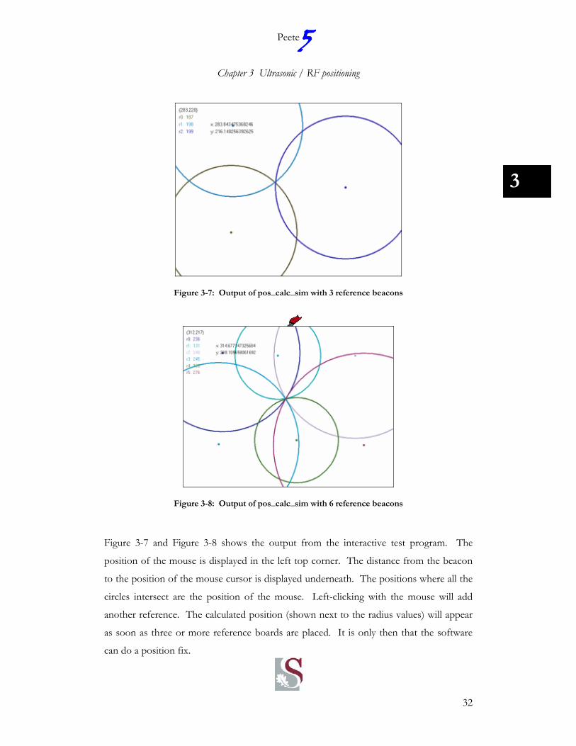
Figure 3-8: Output of pos_calc_sim with 6 reference beacons

Figure 3-7 and Figure 3-8 shows the output from the interactive test program. The

position of the mouse is displayed in the left top corner. The distance from the beacon

to the position of the mouse cursor is displayed underneath. The positions where all the

circles intersect are the position of the mouse. Left-clicking with the mouse will add

another reference. The calculated position (shown next to the radius values) will appear

as soon as three or more reference boards are placed. It is only then that the software

can do a position fix.

5Peete


33

3

Noise is added to the radius measurements. The noise levels can be changed in the

software. When more beacons are added (as in Figure 3-8), the noise on the calculated

position comes down although the noise on the radius measurements stays the same.

Figure 3-9 shows the output from the second simulation program. In this case, it took

the data from an actual test setup and calculated the robot’s position. The blue squares

on the edges of the plots show the position of the beacons. The cluster of points is the

positions calculated by the robot.

Left: 80mm noise on the measurement. Right: 10mm noise on the measurement

Figure 3-9: Position calculation with three beacons.

Figure 3-9 shows the position calculation with only three beacons. Note that with 80mm

of noise on the distance measurement there is an error of almost 200mm in the Y-axis,

and only 100mm in the X-axis. The reason for this difference is the placement of the

reference sensors. The two circles from the top and the bottom beacon would intersect

with a greater area than the two circles from the left and bottom beacon. This is

illustrated better in Figure 3-10 below. Both distance calculations use the same beacons

and the same noise (ε) on the measurement. However, there is a greater error in the X-

axis of the left measurement than in the right measurement. The reason for this is the

area that overlaps both the measurements.

Robot Position

Y [mm]2,1002,0502,0001,9501,9001,8501,8001,7501,7001,650

X [m

m]

1,400

1,350

1,300

1,250

1,200

1,150

1,100

1,050

1,000

950

900

850

800

750

700

650

600

550

Robot Position

Y [mm]2,0001,9501,9001,8501,8001,7501,7001,650

X [m

m]

1,400

1,350

1,300

1,250

1,200

1,150

1,100

1,050

1,000

950

900

850

800

750

700

650

600

550

5Peete


34

3

ε

Large area.

ε Small area.

Figure 3-10: Dependence of position error on beacon placement

One way of limiting this error would be to add another beacon. This is shown in Figure

3-10 where a fourth beacon was added. The error in the X-axis and Y-axis are now

almost identical.

Left: 80mm noise on the measurement. Right: 10mm noise on the measurement

Figure 3-11: Position calculation with four beacons.

Robot Position

Y [mm]2,6002,4002,2002,0001,800

X [m

m]

1,400

1,350

1,300

1,250

1,200

1,150

1,100

1,050

1,000

950

900

850

800

750

700

650

600

550

Robot Position

Y [mm]2,6002,4002,2002,0001,800

X [m

m]

1,400

1,350

1,300

1,250

1,200

1,150

1,100

1,050

1,000

950

900

850

800

750

700

650

600

550

5Peete


35

3

3.4 Ultrasonic Positioning

3.4.1 Concept

The reason why ultrasonic range finding was used as opposed to conventional RF or

infrared methods is mainly because of affordability and the speed of sound. Sound

waves travel at 343m/second (see [10]) in air at room temperature (20°C). This can be

seen as relatively slow compared to the speed of modern processors and negligible

compared to the speed of light. It is effectively the difference between the speed of

sound and the speed of light that is used to calculate the distance between the transmitter

and the receiver.

distan

ce

Robot with receiver

Reference / Transmitter

1

2

Figure 3-12: Simplified range finding system

Figure 3-12 shows the concept behind the ultrasonic range finding. If the robot wants to

know how far it is from a certain reference board, the following steps will be performed:

1. The robot will send a message (over the RF link) to the reference board,

requesting an ultrasonic pulse to be sent.

2. On receiving the request, the reference board will acknowledge the request (again

over the RF link), and at the same time transmit an ultrasonic pulse. The RF

5Peete


36

3

signal will travel much faster than the ultrasonic one, and its propagation time

delay can be neglected.

3. When the robot receives the reply from the reference board, it will signal its

secondary RX DSP over the CAN bus to start looking for the pulse. The RX

DSP will demodulate the received signal, and pass back the distance measured to

the main DSP.

The range information can now be used in equation 3-9 to calculate the position of the

robot.

3.4.2 Simple solution

The simplest solution would be to transmit an ultrasonic pulse on a specific carrier wave

(CW). The length of the pulse is of little importance and can possibly only be long

enough to get the maximum power out of the transducer.

The detection circuit in this case will also be quite simple. A band pass filter with a level

detection circuit should do the job. The receiver would have to measure the time from

when the signal was sent (as signalled by the transmitter over the RF link) until its

threshold circuit was triggered.

5Peete


37

3 0 200 400 600 800 1000

-2

-1

0

1

2

Time

Vol

ts [V

]

0 0.5 1 1.5 2

x 105

-100

-50

0

50

Freq [Hz]

Pow

er [d

B]

0 200 400 600 800 1000-0.01

-0.005

0

0.005

0.01

Time

Vol

ts [V

]

0 0.5 1 1.5 2

x 105

-180-160-140-120-100-80-60

Freq [Hz]

Pow

er [d

B]

0 200 400 600 800 1000-10

-5

0

5x 10

-3

Time

Vol

ts [V

]

0 0.5 1 1.5 2

x 105

-180

-160

-140

-120

-100

-80

Freq [Hz]

Pow

er [d

B]

Figure 3-13: Simple ultrasonic measurements

Figure 3-13 shows some measurements that were done with an ultrasonic transmitter and

receiver. A constant CW (40 kHz) was transmitted and the value measured by the

receiver was sampled by an Analogue to Digital Converter (ADC). The sampling rate is

400 kHz. The left hand side graphs show the measured data, while the right hand side

shows the spectrum (Fourier transformation) of the measured data.

Three different setups were used to compare measurements (the results of which are

shown in Figure 3-13):

• The transmitter and the receiver were placed close to each other (about 15cm

apart).

• The transmitter and receiver were placed far apart (> 2m).

• The transmitter was switched off.

5Peete


38

3

The received signal in the first case (receiver and transmitter close together) was very

strong. So much so that it started to saturate the RX amplifier. The effect of the

saturation can be seen in the spectrum where there is a strong signal at 1.2MHz (3 x 40

kHz). The received signal is very strong at about 44dB (this dB value is not an absolute

value but a relative value). Very little filtering is necessary to detect this signal.

In the second case (receiver and transmitter far apart), it is impossible for the human eye

to see the received signal in the raw data. Only when one looks at the spectrum is it

possible to see that there is still a signal at 40 kHz (at -81 dB). The noise floor is at about

-110dB resulting in a signal-to-noise ratio of 30 dB. It is still possible to detect this signal

but the analogue implementation is very difficult.

The biggest hurdle in the analogue path will be the band-pass filter. A 30 dB signal-to-

noise ratio is only possible if a very narrow filter with a high Q is used (an 8 pole

Butterworth filter would be needed). Although it is possible to design such a filter, it is

almost impossible to realize it without very fine tuning. For robust, reliable and sensitive

ultrasonic range determination, a different solution must be found.

3.4.3 Barker code

The previous section showed that a simple solution is unlikely to solve the problem.

Luckily there are tools and devices available today that offer a whole new range of

solutions to the problem. The one chosen for this problem was digital. Working in the

digital domain offers infinitely more possibilities. The implementation of a band-pass

filter becomes trivial while the bandwidth of the filter is determined by the resolution of

the processor. More bits mean smaller values which result in lower bandwidth.

Radar techniques can be implemented with the use of modern day Digital Signal

Processors (DSP). The transmitter can transmit a specially shaped burst of impulses.

5Peete


39

3

The receiver can sample the incoming signal and implement a matched filter by

correlating the signal with the transmitted reference signal.

The question now is what kind of filter (or impulse stream) to use. One solution would

be to use a pseudo-random sequence of impulses to modulate the phase of the carrier

wave. A 10-bit random stream will look something like [1 0 1 1 0 1 0 0 0 1]. A 1 will

represent a 0 degree phase in the transmitted signal while a 0 represents a 90 degree

phase in the transmitted signal. If the receiver correlates the incoming signal with the

same stream used by the transmitter, then you have a matched filter.

Figure 3-14 shows the autocorrelation of various lengths of random impulses. This

simulation was done in Matlab.4

0 5 10 15 200

1

2

3

4Correlation with 10 random bits

0 10 20 30 400

2

4

6

8

10


0 20 40 60 800

5

10

15

20


0 50 100 1500

5

10

15

20

25

30


Figure 3-14: Autocorrelation of different length random streams

4 The source code can be found in \programming\Matlab

5Peete


40

3

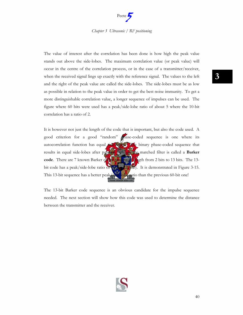
The value of interest after the correlation has been done is how high the peak value

stands out above the side-lobes. The maximum correlation value (or peak value) will

occur in the centre of the correlation process, or in the case of a transmitter/receiver,

when the received signal lings up exactly with the reference signal. The values to the left

and the right of the peak value are called the side-lobes. The side-lobes must be as low

as possible in relation to the peak value in order to get the best noise immunity. To get a

more distinguishable correlation value, a longer sequence of impulses can be used. The

figure where 60 bits were used has a peak/side-lobe ratio of about 5 where the 10-bit

correlation has a ratio of 2.

It is however not just the length of the code that is important, but also the code used. A

good criterion for a good “random” phase-coded sequence is one where its

autocorrelation function has equal side-lobes. The binary phase-coded sequence that

results in equal side-lobes after passage through the matched filter is called a Barker

code. There are 7 known Barker codes ranging in length from 2 bits to 13 bits. The 13-

bit code has a peak/side-lobe ratio of 13 (or 22.3dB). It is demonstrated in Figure 3-15.

This 13-bit sequence has a better peak/side-lobe ratio than the previous 60-bit one!

The 13-bit Barker code sequence is an obvious candidate for the impulse sequence

needed. The next section will show how this code was used to determine the distance

between the transmitter and the receiver.

5Peete


41

3

0 50 100 150 200 250 300 350 400 4500

20

40

60

80

100

12013-bit Barker code autocorrelation

Figure 3-15: 13-bit Barker code autocorrelation

3.4.4 Simulation

Various methods were investigated to find the best way of simulating the complete

transmit/receive path. Matlab is an obvious candidate because of its powerful use of

matrices and the built-in functions. A lot of the initial work was done in Matlab5 but the

final solution was implemented in Delphi6. The reason for this is that it also made it

easier to port the final solution to C or assembler in the embedded code.

More than one simulation program was written in Delphi. It started with a simple

simulation program where all the variables were fixed. This soon created limitations

when trying to understand the effects in the actual transmission. A more flexible and

tuneable program was needed and the specifications of a final simulation program were

written down:

5 The matlab examples can be found in \programming\matlab\ 6 Delphi is an Object Oriented programming language based on Pascal.

5Peete


42

3

• All the major variables (ultrasonic frequency, sampling rate, noise, etc.) must be

configurable at run time.

• It had to simulate the whole system, from transmitter up to the final peak

detection in the receiver.

• The bandwidth of the ultrasonic transducers had to be simulated.

• All the measurable points in the system must be captured to be displayed on a

graph or exported to a file for later analysis.

The program u_sonic_sim.exe was developed for simulating the complete system7. It

meets all the requirements mentioned above.

tx_code modulated_tx_code

tx_signal

noise,time delay

rx_signal

ADC samplerFirst

correlationsecond

correlation

Transmitter Transmissionmedium

Receiver

Figure 3-16: Complete ultrasonic system

Figure 3-16 shows the complete ultrasonic system that was simulated. The system is

divided in to three main parts:

• Transmitter – The part of the system responsible for generating and transmitting

the barker-coded impulses.

• Transmission medium – This will be the air that the ultrasonic signal passes

through.

• Receiver – The part of the system responsible for receiving and demodulating the

transmitted signal.

7 The program can be found in \usonic\programming\delphi\usonic sim\

5Peete


43

3

These three systems in turn contain various parts. Some will be hardware (e.g. ultrasonic

transducers), and some software (e.g. modulated barker code). The purpose of the

simulation software was to implement and simulate all of these.

The rest of this section will explain the ultrasonic solution in detail by explaining all of

the different parts in the simulation (refer to Figure 3-16).

TX CODE

The tx_code is the code used to modulate the signal by. In this case, it will be the Barker

code: [1 1 1 1 1 0 0 1 1 0 1 0 1]. The code sequence is adjustable and allows the

investigation of different code sequences. A plot of the generated tx_code is shown in

Figure 3-17.

0 1 2 3 4 5 6 7 8 9 10-1

-0.8

-0.6

-0.4

-0.2

0

0.2

0.4

0.6

0.8

1gen tx code

time [ms]

Figure 3-17: Generated TX code

5Peete


44

3

MODULATED TX CODE

0 0.5 1 1.5 2 2.5 3 3.5 4

-1

-0.8

-0.6

-0.4

-0.2

0

0.2

0.4

0.6

0.8

1

gen modulated TX

time [ms]

Figure 3-18: Modulated TX signal

A 40 kHz carrier wave is used to transmit the ultrasonic signal. This signal is phase

modulated by the tx_code. The resulting signal is shown in Figure 3-18. It is very

difficult to see in this small picture, but if one looks closely, then the 180 degree phase

changes can be seen.

This signal is the final signal generated by the transmitter in software. It will now be used

to drive external hardware in order to transmit the signal via the ultrasonic transducer.

5Peete


45

3

TRANSMITTED SIGNAL

1 2 3 4 5 6 7 8

x 104

-10

0

10

20

30

40

Freq [Hz]

Pow

er

Spectrum of modulated TX signal

Figure 3-19: Spectrum of modulated TX signal

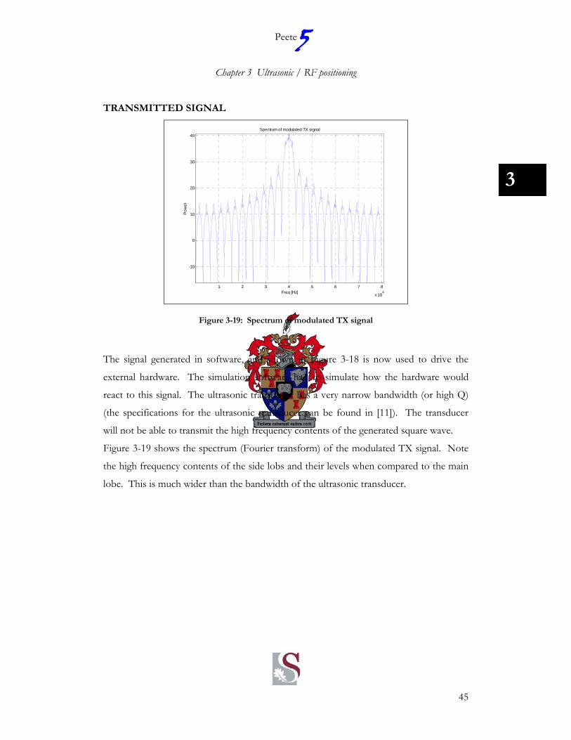
The signal generated in software, and shown in Figure 3-18 is now used to drive the

external hardware. The simulation software had to simulate how the hardware would

react to this signal. The ultrasonic transducer has a very narrow bandwidth (or high Q)

(the specifications for the ultrasonic transducer can be found in [11]). The transducer

will not be able to transmit the high frequency contents of the generated square wave.

Figure 3-19 shows the spectrum (Fourier transform) of the modulated TX signal. Note

the high frequency contents of the side lobs and their levels when compared to the main

lobe. This is much wider than the bandwidth of the ultrasonic transducer.

5Peete


46

3 0 0.5 1 1.5 2 2.50.5

1

1.5

2

2.5

3x 10

4

time [ms]

Ultrasonic pulse

Raw

AD

C v

alue

30 40 50 60 70 80 9080

90

100

110

120

130

140

Freq [kHz]

Pow

er

Spectrum of ultrasonic pulse

Figure 3-20: Ultrasonic pulse and its spectrum

A simple measurement was made to determine the bandwidth of the ultrasonic

transducer. A single ultrasonic pulse was sent, and the received signal was measured.

The received signal is shown in the top half of Figure 3-20. The spectrum of this signal

is shown in the bottom half. Note the transient response of the received signal. This is

because of the bandwidth of the transmitter and receiver.

The simulation program had to take this bandwidth of the transducer in to account in

order to get a reasonable representation of the final system. In order to achieve this, the

modulated TX signal was sent through a band pass filter (the implementation of an IIR

filter is given in APPENDIX A) to simulate the response of the ultrasonic transducer.

The resulting signal is shown in Figure 3-21. The phase transitions are now more clearly

defined because of this bandwidth limitation. Clear gaps are seen where the phase

changes from 0 degrees phase to 180 degrees phase.

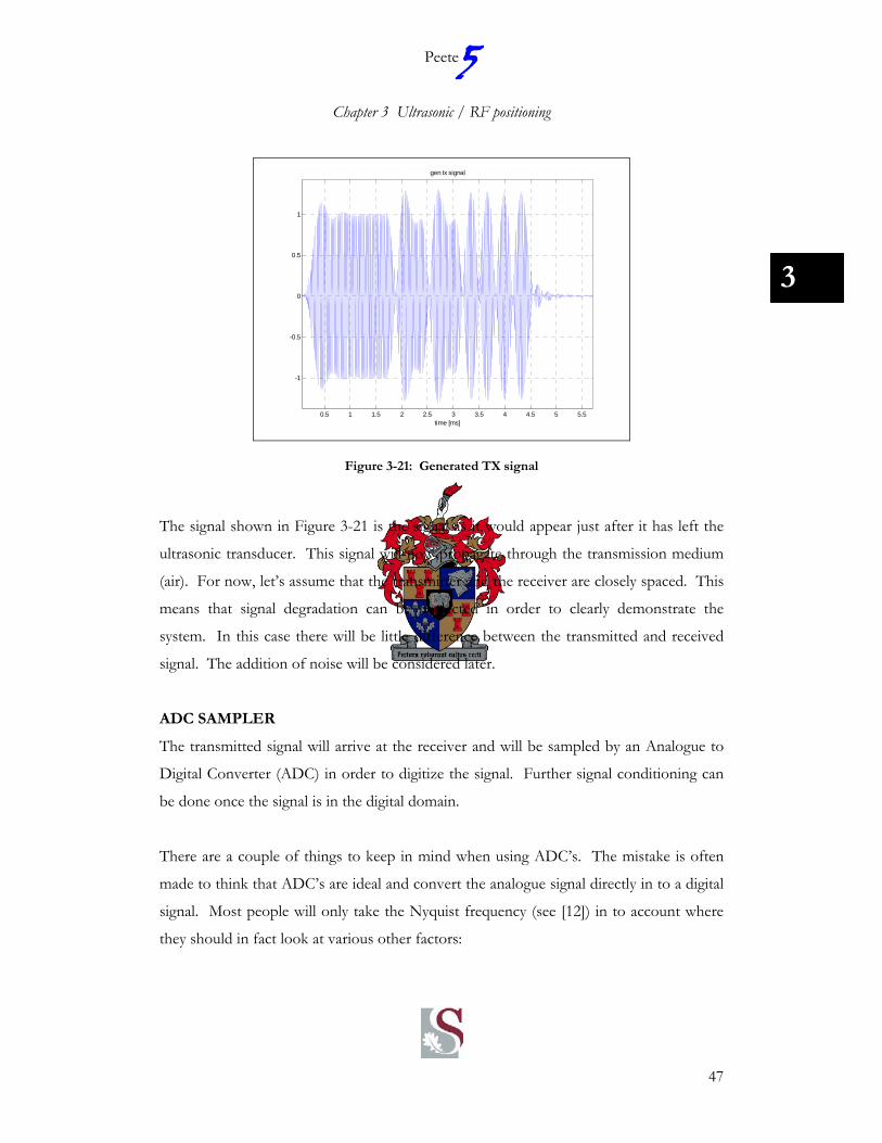
5Peete


47

3

0.5 1 1.5 2 2.5 3 3.5 4 4.5 5 5.5

-1

-0.5

0

0.5

1

gen tx signal

time [ms]

Figure 3-21: Generated TX signal

The signal shown in Figure 3-21 is the signal as it would appear just after it has left the

ultrasonic transducer. This signal will now propagate through the transmission medium

(air). For now, let’s assume that the transmitter and the receiver are closely spaced. This

means that signal degradation can be neglected in order to clearly demonstrate the

system. In this case there will be little difference between the transmitted and received

signal. The addition of noise will be considered later.

ADC SAMPLER

The transmitted signal will arrive at the receiver and will be sampled by an Analogue to

Digital Converter (ADC) in order to digitize the signal. Further signal conditioning can

be done once the signal is in the digital domain.

There are a couple of things to keep in mind when using ADC’s. The mistake is often

made to think that ADC’s are ideal and convert the analogue signal directly in to a digital

signal. Most people will only take the Nyquist frequency (see [12]) in to account where

they should in fact look at various other factors:

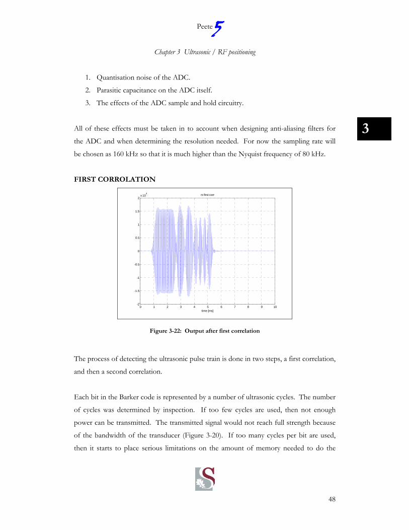
5Peete


48

3

1. Quantisation noise of the ADC.

2. Parasitic capacitance on the ADC itself.

3. The effects of the ADC sample and hold circuitry.

All of these effects must be taken in to account when designing anti-aliasing filters for

the ADC and when determining the resolution needed. For now the sampling rate will

be chosen as 160 kHz so that it is much higher than the Nyquist frequency of 80 kHz.

FIRST CORROLATION

0 1 2 3 4 5 6 7 8 9 10-2

-1.5

-1

-0.5

0

0.5

1

1.5

2x 10

4 rx first corr

time [ms]

Figure 3-22: Output after first correlation

The process of detecting the ultrasonic pulse train is done in two steps, a first correlation,

and then a second correlation.

Each bit in the Barker code is represented by a number of ultrasonic cycles. The number

of cycles was determined by inspection. If too few cycles are used, then not enough

power can be transmitted. The transmitted signal would not reach full strength because

of the bandwidth of the transducer (Figure 3-20). If too many cycles per bit are used,

then it starts to place serious limitations on the amount of memory needed to do the

5Peete


49

3

correlation. The simulation program does allow the changing of the number of

cycles/bit in order to find a good solution.

The first correlation is used to detect the presence of one code bit. The length of this

correlation must be the number of cycles/bit multiplied by the number of samples per

cycle.

For example:

If the number of cycles/bit is 20 and the sampling rate is 160 kHz, then the number of

samples per cycle is 4, and the length of the first correlation is 80.

The values (or taps) of this correlation will simply be the signal that is being detected,

namely one bit. This means that it is merely a 40 kHz sine wave sampled at 160 kHz.

The presence of a bit will be detected when the output of this correlation peaks. A

positive output means a bit with a 0 degree phase while a negative output means a bit

with a 180 degree phase.

0 0.1 0.2 0.3 0.4 0.5 0.6 0.7 0.8 0.9 1-30

-20

-10

0

10

20

30

40

Normalized Angular Frequency (×π rads/sample)

Mag

nitu

de (d

B)

0 0.1 0.2 0.3 0.4 0.5 0.6 0.7 0.8 0.9 1-1500

-1000

-500

0

500

Normalized Angular Frequency (×π rads/sample)

Pha

se (d

egre

es)

Figure 3-23: FIR filter response

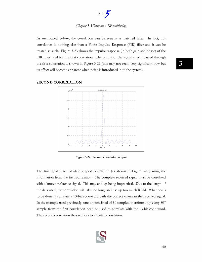
5Peete


50

3

As mentioned before, the correlation can be seen as a matched filter. In fact, this

correlation is nothing else than a Finite Impulse Response (FIR) filter and it can be

treated as such. Figure 3-23 shows the impulse response (in both gain and phase) of the

FIR filter used for the first correlation. The output of the signal after it passed through

the first correlation is shown in Figure 3-22 (this may not seem very significant now but

its effect will become apparent when noise is introduced in to the system).

SECOND CORRELATION

0 1 2 3 4 5 6 7 8 9 100

0.5

1

1.5

2

2.5

3x 10

4 rx second corr

time [ms]

Figure 3-24: Second correlation output

The final goal is to calculate a good correlation (as shown in Figure 3-15) using the

information from the first correlation. The complete received signal must be correlated

with a known reference signal. This may end up being impractical. Due to the length of

the data used, the correlation will take too long, and use up too much RAM. What needs

to be done is correlate a 13-bit code-word with the correct values in the received signal.

In the example used previously, one bit consisted of 80 samples, therefore only every 80th

sample from the first correlation need be used to correlate with the 13-bit code word.

The second correlation thus reduces to a 13-tap correlation.

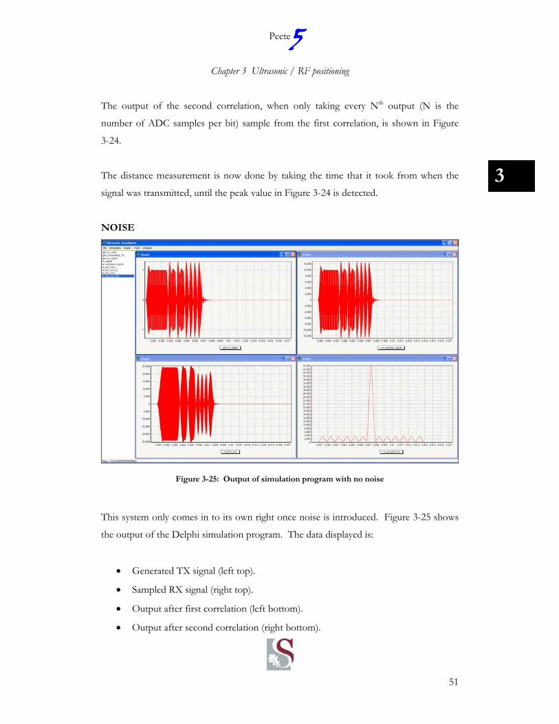
5Peete


51

3

The output of the second correlation, when only taking every Nth output (N is the

number of ADC samples per bit) sample from the first correlation, is shown in Figure

3-24.

The distance measurement is now done by taking the time that it took from when the

signal was transmitted, until the peak value in Figure 3-24 is detected.

NOISE

Figure 3-25: Output of simulation program with no noise

This system only comes in to its own right once noise is introduced. Figure 3-25 shows

the output of the Delphi simulation program. The data displayed is:

• Generated TX signal (left top).

• Sampled RX signal (right top).

• Output after first correlation (left bottom).

• Output after second correlation (right bottom).

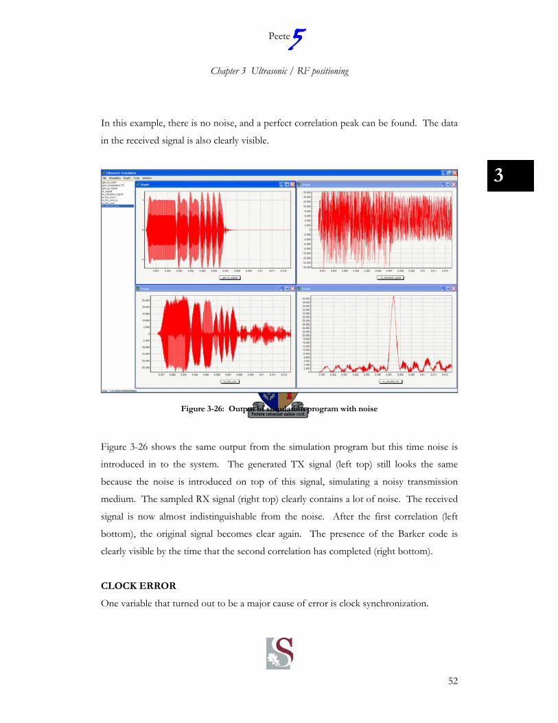
5Peete


52

3

In this example, there is no noise, and a perfect correlation peak can be found. The data

in the received signal is also clearly visible.

Figure 3-26: Output of simulation program with noise

Figure 3-26 shows the same output from the simulation program but this time noise is

introduced in to the system. The generated TX signal (left top) still looks the same

because the noise is introduced on top of this signal, simulating a noisy transmission

medium. The sampled RX signal (right top) clearly contains a lot of noise. The received

signal is now almost indistinguishable from the noise. After the first correlation (left

bottom), the original signal becomes clear again. The presence of the Barker code is

clearly visible by the time that the second correlation has completed (right bottom).

CLOCK ERROR

One variable that turned out to be a major cause of error is clock synchronization.

5Peete


53

3

In order to demodulate the signal correctly, the transmitter and receiver must have their

clock sources as close as possible to one another.

Figure 3-27 shows the same simulation as above but with a clock error between the

transmitter and receiver. In this case, a clock error of only 1% between the transmitter

and the receiver was used. Although the first correlation still looks acceptable, the phase

of the signal is slowly drifting. The phase information is the information used to decode

the bit stream, and is crucial for the second correlation. By the time that the second

correlation has been performed, the data is completely useless.

Figure 3-27: Output of simulation program with clock error of 400 Hz

The clock error can be corrected in two ways:

• Use a more accurate (and expensive) clock source.

• Implement a Phase Lock Loop (PLL) to compensate for the clock error.

5Peete


54

3

The second method of a PLL was implemented and tested but required too much

program RAM. The final hardware solution was to use a more accurate clock source.

The simulation program contains many other features including:

• Adjustable sampling rate.

• Different filters for simulating the ultrasonic transducer.

3.4.5 Implementation

This section will explain how the information gained from the Delphi simulation was

used to implement the actual range finding system in the microcontrollers. The concept

is simple:

1. Sample the received signal.

2. Perform the first correlation every time a new value is sampled and store a result

long enough to hold the complete Barker code.

3. Take every Nth sample from the first correlation, and correlate it with the Barker

code.

4. Maintain a counter and store its value every time that a peak is detected from the

second correlation. This counter can later be used to determine the time delay

between transmission and reception.

This all sound fine in theory, but there are some serious limitations when it comes to

implementing it. The greatest of these is the time available. The complete first and

second correlation must be done every time that a new value is sampled. If the first

correlation contains 80 taps, and the second contains 13 taps, then 93 multiplications and

additions are needed for every sample. The sampling rate chosen is 160 kHz meaning

that all the processing must be done in less than 6.25µs! This is very little time in deed.

It would be impossible to do this with normal C code and a standard 8-bit

microcontroller.

5Peete


55

3

The DSP56F8xxE series of DSP’s from Freescale was chosen for use in Peete5. The

following features of the DSP make it ideal for the range finding problem:

• DSP functionality needed for implementing FIR filters, IIR filters, correlations,

etc.

• 16-bit processor for high resolution processing.

• 12-bit ADC converters.

• Enough RAM and ROM.

• 60 Million Instructions per Second (MIPS).

• Complementary pair Pulse Width Modulators (PWM).

• Quad Timer Module.

With this DSP running at 60 MIPS, there are 375 clock cycles available per ADC sample

taken. Although this may sound like enough, not all instructions execute in 1 clock cycle.

Thorough knowledge of the DSP is needed in order to program it in its assembler

language. The user manual [14] and family manual [13] can be consulted for more

information.

The next two sections will explain how the DSP was used in both the transmitter and the

receiver.

1.1.1.1. Transmitter

The transmitter is the simpler part of the solution. It needs to generate the modulated

TX signal shown in Figure 3-18. The following DSP peripherals are used in order to

achieve this:

• Pulse Width Modulator.

• Quad timer module.

Pulse Width Modulator

The interface between the DSP and the ultrasonic transducer is explained later in 4.8.

5Peete


56

3

This interface requires two signals to drive the ultrasonic transducer. The two signals

must be 180 degrees out of phase (when the one is high, the other must be low and vice-

versa). The frequency of these two signals determines the ultrasonic transmission

frequency and must be 40 kHz. There must also be some dead-time between the

transitions of these two signals.

All these requirements are met by the PWM used. The PWM has certain control

registers that control its functionality. These registers were set up to:

• Work in complementary pair mode.

• Have a duty cycle of 50%.

• Have frequency of 40 kHz.

• Have a dead time of 500ns between transitions.

The phase of the two complementary signals can be changed with a single control bit.

This makes it very easy to insert the 180 degree phase required for the transmitted signal.

Quad Timer Module

The Quad Timer Module is a module that contains 4 timer modules that can function

either independently or connected to one another. A single timer is needed to generate

the TX pulse. This timer needs to count only the length of 1 bit and will be used to

transmit the 13 Barker code bits.

Figure 3-28 shows how the timer and PWM are used to generate the modulated TX

signal.

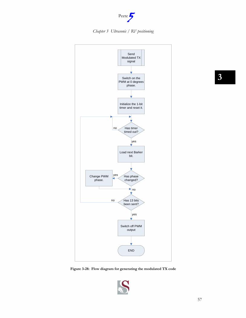
5Peete


57

3

Send Modulated TX

signal

Switch on the PWM at 0 degrees

phase.

Initialize the 1-bit timer and reset it.

Has timer timed out?

Load next Barker bit.

Has phase changed?

Has 13 bits been sent?

Change PWM phase.

yes

no

yes

END

yes

no

no

Switch off PWM output

Figure 3-28: Flow diagram for generating the modulated TX code

5Peete


58

3

1.1.1.2. Receiver

The receiver does not only use the peripherals of the DSP but also many of its DSP

functions.

The peripherals used are:

• Quad Timer Module.

• ADC converter.

Quad Timer Module

More than one timer is needed for the receiver. These timers perform the following

functions:

1. Generate the 160 kHz interrupts needed to sample the incoming signal.

2. Limit the duration of the receiving process. The receiver does not continue to try

and demodulate a received signal indefinitely. A time constraint was placed on

the receiver. The time that it takes for an ultrasonic signal to travel 5 meters was

used.

ADC converter

The ADC converter was set up to sample a single sample at the maximum conversion

time whenever it received a synchronization pulse. The synchronization pulse was

generated by one of the Timer Modules.

The flow diagram in Figure 3-29 shows the demodulating process. The two blocks of

most interest is the two correlation blocks. The correlation equation is given by:

∑−

=

−⋅=1

0

)()()(M

k

knxkcny

3-11

5Peete


59

3

Where:

• y(n) is the output of the correlation function.

• x(n) is the input signal

• M is the number of taps of the correlation.

• c(k) is the taps of the correlation.

This equation could be implemented as it is in the Delphi code because all the previous

data of x(n) is stored. This result in a huge number of data that needs to be stored and is

clearly impractical for implementation in the DSP with limited RAM. Inspection of the

equation shows that the input information before (n-M-1) is not used. This means that

this data does not have to be stored. The question now is: how does one implement

this?

The solution is to use a circular buffer for storing input and output values. If the

correlation has a length of M, then only M words needs to be stored. As soon as the

M+1 input is measured, the value at location 0 can be erased, for the M+2 input, the

location at 1, etc. In this way, only M words are stored at a given time.

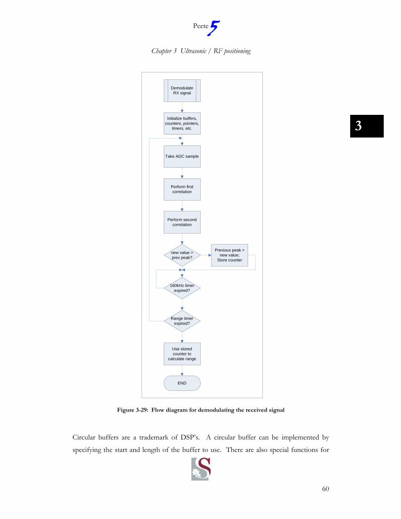
5Peete


60

3

Demodulate RX signal

Initialize buffers, counters, pointers,

timers, etc.

Take ADC sample

Perform first correlation

Perform second correlation

new value > prev peak?

Previous peak = new value;

Store counter

160kHz timer expired?

Range timer expired?

Use stored counter to

calculate range

END

Figure 3-29: Flow diagram for demodulating the received signal

Circular buffers are a trademark of DSP’s. A circular buffer can be implemented by

specifying the start and length of the buffer to use. There are also special functions for

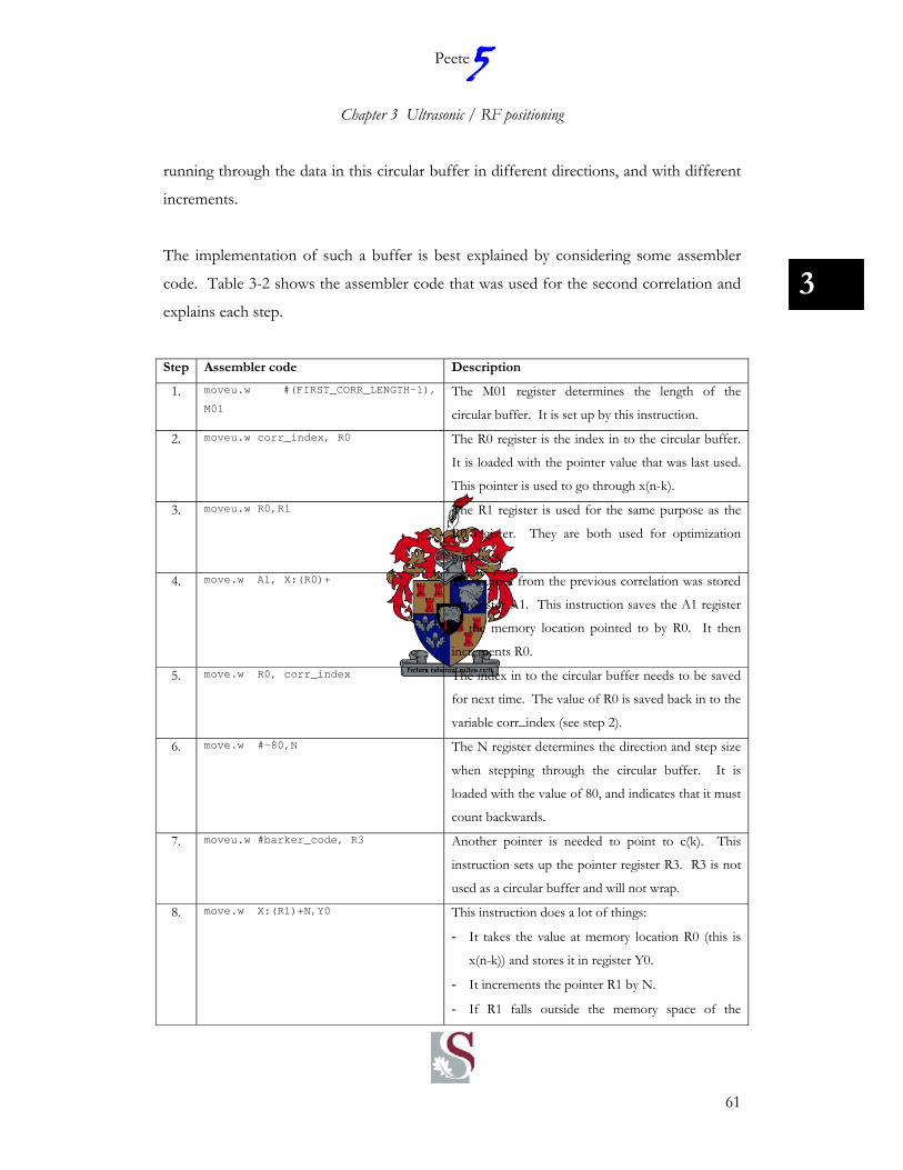
5Peete


61

3

running through the data in this circular buffer in different directions, and with different

increments.

The implementation of such a buffer is best explained by considering some assembler

code. Table 3-2 shows the assembler code that was used for the second correlation and

explains each step.

Step Assembler code Description

1. moveu.w #(FIRST_CORR_LENGTH-1),

M01

The M01 register determines the length of the

circular buffer. It is set up by this instruction.

2. moveu.w corr_index, R0 The R0 register is the index in to the circular buffer.

It is loaded with the pointer value that was last used.

This pointer is used to go through x(n-k).

3. moveu.w R0,R1 The R1 register is used for the same purpose as the

R0 register. They are both used for optimization

purposes.

4. move.w A1, X:(R0)+ The output from the previous correlation was stored

in register A1. This instruction saves the A1 register

to the memory location pointed to by R0. It then

increments R0.

5. move.w R0, corr_index The index in to the circular buffer needs to be saved

for next time. The value of R0 is saved back in to the

variable corr_index (see step 2).

6. move.w #-80,N The N register determines the direction and step size

when stepping through the circular buffer. It is

loaded with the value of 80, and indicates that it must

count backwards.

7. moveu.w #barker_code, R3 Another pointer is needed to point to c(k). This

instruction sets up the pointer register R3. R3 is not

used as a circular buffer and will not wrap.

8. move.w X:(R1)+N,Y0 This instruction does a lot of things:

- It takes the value at memory location R0 (this is

x(n-k)) and stores it in register Y0.

- It increments the pointer R1 by N.

- If R1 falls outside the memory space of the

5Peete


62

3

circular buffer (determined by register M01) then

R1 is wrapped correctly in to the correct memory

space again.

9. clr A X:(R3)+, X0 This instruction does even more:

- It clears the 32-bit result register A.

- Takes the value at memory location R3 (this is

c(k)) and stores it in register Y0.

- Increments (but does not wrap) R3 by 1.

10. rep #13

mac Y0,X0,A X:(R1)+N,Y0 X:(R3)+,X0

The next instruction is repeated 13 times (to do the

13-tap correlation) and performs the following tasks:

- It multiply registers Y0 and X0 with each other

(c(k) * x(n-k) ) and adds the result to register A.

- It takes the next value (x(n-k) ) out of the circular

buffer at location R0, and store the result in Y0.

- It increments and wraps register R1 as it did in

step 8.

- It takes the next value (c(k) ) and stores it in

register X0.

- It increments register R3.

Table 3-2: Explanation of second correlation assembler code

1.1.1.3. Time synchronization

The distance measurement is made by measuring the time between transmitting the

signal and receiving it. One requirement in this scheme is that the receiver knows exactly

when the transmitter sends the pulse. Any error in this time will result in a distance

measurement error. There are 2 timing variables:

1. Time that the transmitter takes to start sending the ultrasonic pulse after it has

signalled to do so over the RF link.

2. Time that the main DSP takes to signal the RX DSP after it has received

confirmation from the TX DSP.

5Peete


63

3

The length of these two times does not matter as it can be incorporated in to the distance

calculation. What is important is that it stays constant for each measurement. This is not

very difficult to do, but will result in errors if not taken in to account. The following

measures were taken to ensure that the time remains constant:

• The TX DSP uses a transmitter empty interrupt on its SCI port to know when

the last byte has been sent over the RF link. Only once this interrupt has

triggered does it immediately start to transmit the ultrasonic pulse.

• The TX DSP disables all interrupts while it is busy sending an ultrasonic pulse to

ensure correct timing.

• The Main DSP parses the received RF packet immediately and sends a

notification to the RX DSP over the CAN interface.

• A separate CAN pipe is used to signal ultrasonic events. This ensures that the

message gets through even if another CAN message is being transmitted.

3.4.6 Distance Calibration

The output from the distance measurement is the value of a counter when the peak

correlation value occurred. This counter value can be converted to a time delay by

multiplying it with the sampling period (1/160 kHz). The time can then be used by the

following equation to determine the distance between the transmitter and receiver:

ε+×= measuredsound tvdist

3-12

Where:

• dist is the distance measured [in meters]

• vsound is the speed of sound.

• tmeasured is the time measured by using the peak counter.

• ε is an error term. This will include the timing caused by the communication

delays on the RF link.

5Peete


64

3

This equation was implemented and the speed of sound was verified to make sure that

the system worked as predicted. This solution requires two steps in software:

1. Converting the counter value to a time value.

2. Calculating the distance with the time value.

It was later replaced for a quicker and more robust solution. This solution took the

counter value and converts it directly to a distance by implementing the following

equation for a straight line:

cxmy +⋅=

3-13

Where:

• m is the slope of the line.

• c is the offset of the line.

980 1000 1020 1040 1060 1080 1100 1120 1140 1160750

800

850

900

950

1000

1050

1100

1150

1200

Correlation peak counter

Dis

tanc

e [m

m]

Figure 3-30: Correlation peak counter over distance

Figure 3-30 shows a plot of the correlation peak counter against the distance between the

transmitter and the receiver. The points measured forms a straight line. A least-squares

estimate was done on the data to determine the values of m and c for the line. These

5Peete


65

3

values were then programmed in to the RX DSP and it could use the equation 3-13 for a

straight line to convert the counter value directly to a distance measurement.

3.5 Conclusion

The simulation methods used for the ultrasonic transmitter and receiver were a great

success. One of the features not mentioned under simulation was that the output of the

PC simulation could be used to test the embedded software. The exact same results were

obtained to prove that the algorithms were working. A measurement was then made to

use actual data for the embedded receiver simulation. Again the results agreed exactly

with those of the simulation.

The results of Figure 3-30 show how well the system worked. The system is completely

linear and can work as long as there is a good signal to noise ratio. Failure of the system

occurs only when the output of the second correlation falls below the noise floor.

One of the problems encountered when testing the system was multi-path. This is where

a reflected signal from the transmitter arrives only slightly later at the receiver than the

actual signal. The second reflected signal contains all the information of the actual signal

and causes errors in the receiver. It would manifest itself as an offset in the distance

measurement. This was not a major problem though since the transmitters and receiver

could be placed in such a way that the direct signal would always be much stronger than

any reflected signal. It is a problem though that may be addressed in future revisions of

this system.

The system worked reliably over the required distances and could be used for the

position control algorithms explained in the previous chapter.

This system required complicated and powerful hardware. The design of the electronic

hardware is explained in the next chapter.

Chapter 4 Electronic Design

4.1 Introduction

The main goal of this thesis was to develop an absolute

positioning system. The system described in Chapter 3

would have been impossible to develop without a good

and solid electronic design. This chapter will explain

the design decisions made when designing the

electronic circuits for Peete5.

Peete5 contains state of the art micro machined

reference sensors, two high speed and modern DSP’s, stepper motor drivers capable of

controlling the motors at high speed and high accuracy to name just a few.

This chapter will start with a block diagram of the electronic circuit used for Peete5. The

functionality of the different components in the block diagram will be explained as well

as the design process followed to develop and test the electronics.

The same Printed Circuit Board (PCB) can be used for three different purposes

depending on how it is populated with components. The functionality of each one of

these different modules and how they share the basic design will also be explained.

5

Peete


67

4

4.2 PCB Block Diagram

Figure 4-1: Motherboard block diagram

Figure 4-1 shows the block diagram of the Printed Circuit Board (PCB) used in Peete5.

Different configurations of this PCB allow it to be used for either one of the following

purposes:

• Peete5 Motherboard

Almost all the items shown in the block diagram in Figure 4-1 are populated in

this configuration. The only exclusion is the Ultrasonic TX block that is

responsible for converting the signals generated by the Main CPU into ultrasonic

5

Peete


68

4

pulses. The motherboard does not need to transmit pulses and it is therefore

omitted.

• Peete5 Transmitter Board

The transmitter board is responsible for transmitting ultrasonic pulses on request.

It contains only the Main CPU, Ultrasonic TX block, RF transceiver and power

supply. The USB section is optional and can be used when debugging the

system.

The PCB contains the following components:

• Main CPU

• RX DSP

• USB Connector

• Power Connector

• USB to UART converter

• Power Supply (12V; 5V; 3.3V)

• Stepper Motor drivers

• Ultrasonic transmit circuitry

• Ultrasonic transducer

• Ultrasonic receive circuitry

• RF Transceiver

• Rate Gyro and low pass filter

• Inclinometer and low pass filter

• Servo motor

• Interfaces to connect to a video camera and video transmitter

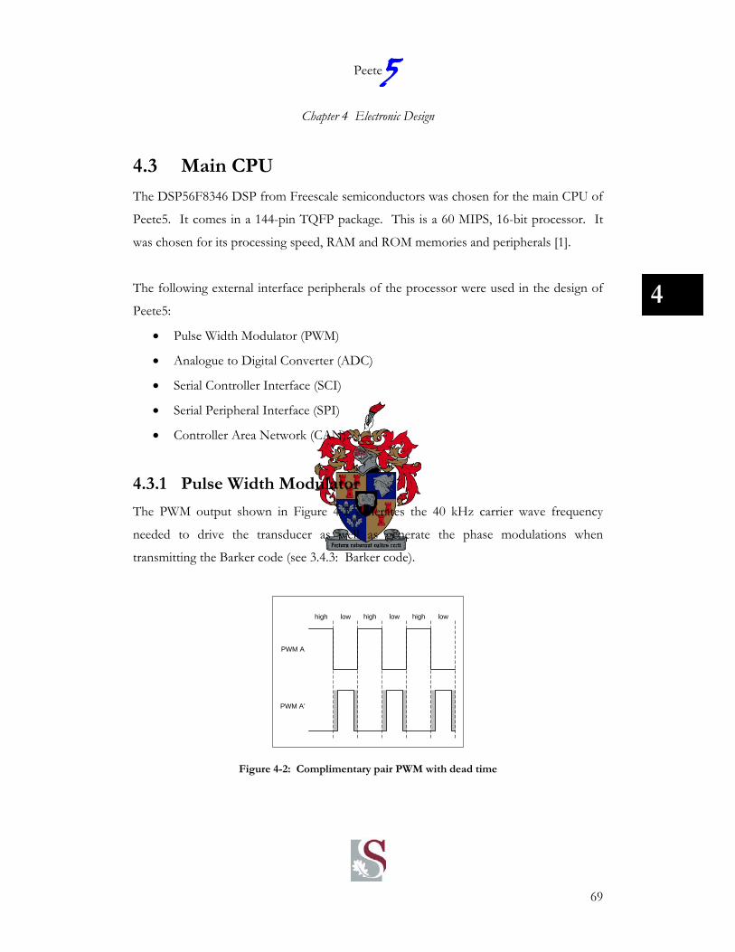
5

Peete


69

4

4.3 Main CPU

The DSP56F8346 DSP from Freescale semiconductors was chosen for the main CPU of

Peete5. It comes in a 144-pin TQFP package. This is a 60 MIPS, 16-bit processor. It

was chosen for its processing speed, RAM and ROM memories and peripherals [1].

The following external interface peripherals of the processor were used in the design of

Peete5:

• Pulse Width Modulator (PWM)

• Analogue to Digital Converter (ADC)

• Serial Controller Interface (SCI)

• Serial Peripheral Interface (SPI)

• Controller Area Network (CAN)

4.3.1 Pulse Width Modulator

The PWM output shown in Figure 4-2 generates the 40 kHz carrier wave frequency

needed to drive the transducer as well as generate the phase modulations when

transmitting the Barker code (see 3.4.3: Barker code).

high high highlow low low

PWM A

PWM A’

Figure 4-2: Complimentary pair PWM with dead time

5

Peete


70

4

The constraints placed on the driving logic by the interface circuitry were also met by the

PWM by setting it up in differential pair mode with dead-time insertion. In this mode,

two signals are generated by one PWM module. The one signal is the inverse of the

other. Dead time between the two signals is automatically inserted when a transition

from high to low (or vice versa) occurs. See Figure 4-2. The dead time is configured via

peripheral registers internal to the DSP.

The PWM also has another use. The stepper motor controllers used to drive the stepper

motors have a reference voltage input that is used to control the current through the

stepper motors. This analogue reference voltage is controlled by using one of the PWM

outputs (in independent mode) and passing it through a simple Resistor-Capacitor (RC)

low pass filter with the filter cut-off frequency at least 10 times lower than the PWM

frequency. The analogue voltage to the stepper motor driver could then be controlled by

controlling the duty cycle of the PWM. The output voltage is given by:

DVvout ×= 3.3

4-1

Where:

vout is the analogue voltage to the stepper motor driver.

3.3V is the output-high voltage of the PWM.

D is the duty cycle (in %) of the PWM.

The bandwidth of the analogue output is determined by the cut-off frequency of the low

pass filter.

4.3.2 Analogue to Digital Converter

The DSP56F8346 contains 16 analogue inputs (channels). These 16 channels go through

four multiplexers to be sampled by four 12-bit ADC’s. The ADC’s can be set up to

sample two channels simultaneously or to sample in a pre-determined sequence.

5

Peete


71

4

The ADC’s have a 3.3V voltage reference and are therefore capable of measuring

voltages between 0V and 3.3V. A 12-bit ADC with a theoretical resolution of 800µV is

used. To realize this resolution, there has to be no digital noise coupling in to the

analogue circuitry and the ADC must have a clean power supply.

Figure 4-3: Equivalent circuit for ADC loading

Figure 4-3 was copied form the datasheet of the DSP. It shows an equivalent circuit of

the ADC. This circuit contains:

1. Parasitic capacitance due to package, pin-to-pin and pin-to-package base

coupling.

2. Parasitic capacitance due to the chip bond pad, ESD protection devices and

signal routing.

3. Equivalent resistance for the ESD isolation resistor and the channel select

multiplexer.

4. Sampling capacitor at the sample and hold circuit. Capacitor C1 is normally

disconnected from the input and is only connected to it at sampling time.

The parasitic components and their effects must be well understood for good ADC

design. The following steps were taken to minimize noise on the analogue

measurements:

5

Peete


72

4

1. The ADC has high quality, low ESR 100 nF decoupling capacitors very close to

the pins of the DSP.

2. The power supply to the ADC is filtered through a Capacitor-Inductor low pass

filter for noise reduction on the power supply.

3. A linear regulator is used to power the ADC.

4. The inputs to the ADC is driven by low impedance sources (Operational

Amplifiers) where the output capacitance have been matched to the input

capacitance of the ADC through the process of trail and error.

4.3.3 Serial Controller Interface

The Serial Controller Interface (SCI) is used for general purpose communications. It

uses only two lines for communications. One for transmit and one for receive. The two

devices communicating over this link need to synchronize their clocks for the data

communications. All this is done internally by the DSP hardware. The DSP has two SCI

controllers. Both of these controllers are used to perform the following functions:

• Full-duplex communications between a Personal Computer (PC) and the Main

processor.

• Half-duplex communications on the RF link.

Two low level drivers were developed for the two different SCI interfaces. Both drivers

will buffer data in the transmit (TX) and receive (RX) paths. This is necessary when

running communications on a fast processor. If no buffering were done, it would mean

that the application layer software would have to wait for every byte to be sent before it

can send another. Buffering the data takes the load off the normal software processes.

The buffering is done using different TX and RX interrupts.

5

Peete


73

4

Transmit a message of

length N bytes.

Is SCI TX ready?

Take next byte out of message

packet.

Write byte directly to SCI TX.

END

Place byte in circular buffer

Has N bytes been sent?

yes

yes

no

no

Enable TX ready interrupt

TX ready interrupt

Take next byte out of circular buffer.

Write byte to SCI TX.

END

Has N bytes been sent?

Disable TX ready interrupt

Exit interrupt service routine

no

yes

Figure 4-4: Double buffering for SCI TX

Figure 4-4 shows a simplified flow diagram for the double buffering of data to the SCI.

A similar process will be used on the receive side.

The two SCI drivers (one for the PC communications, and the other for the RF

communications) are very similar except for the fact that the one is full duplex (PC) and

the other is only half duplex (RF link). The SCI driver for the half-duplex RF link also

5

Peete


74

4

contains control software for controlling the CC1000 RF device. This ensures that the

RF link is in the transmit mode whenever the SCI wants to transmit data and that it is in

the receive mode whenever it is ready to receive data. It also monitors the Received

Signal Strength Indicator (RSSI) from the RF device to detect an incoming packet and

enable the SCI receiver.

4.3.4 Serial Peripheral Interface

The Serial Peripheral Interface (SPI) differs from the SCI interface in the fact that it

contains a clock signal in addition to the transmit and receive lines. No synchronization

is therefore necessary between the transmitter and the receiver. As the name suggests,

this interface is still commonly used to control extra peripherals external to the CPU

itself.

The DSP has two SPI ports. These two ports are used to control the stepper motor

drivers that ultimately control the stepper motors. The stepper motor controller uses

two control words to control the current through each of the windings of the stepper

motor. The two control words are maintained from the low level motor drivers.

It is necessary to meet the timing requirements on the SPI bus of the stepper motor

driver. The timing is controlled by means of special control registers for the SPI. The

highest possible bit rate is used to ensure that the time taken to update the control words

of the stepper motor driver is less that the update period needed to update the currents

in the motors.

4.3.5 Controller Area Network

The Controller Area Network (CAN) is a network protocol interface that has been

developed by Bosch for high speed, high reliability data communications between two or

more processors connected on the same network. The specifications of the CAN

protocol can be found in the Bosch CAN spec [5].

5

Peete


75

4

The CAN bus implements a half-duplex communication link. It is used on Peete5 to

connect the Main CPU and the RX CPU. There is no need for a bus driver since these

two devices are the only devices on the CAN bus. The TX and RX lines of the two

processors are connected together forming a single wire communication bus. The bus

communication speed is determined by the parasitic capacitance on the CPU and a pull

up resistor. The timing of a single CAN bit is controlled via numerous DSP control

registers. These registers determine sample period, sampling time, synchronization width

and propagation delay. A spread sheet was used to calculate these values. The

considerations when setting up a CAN bus can be found in [7].

4.4 RX DSP

The RX DSP has only one purpose and that is to demodulate the incoming ultrasonic

signal and present a distance measurement to the main DSP. The DSP56F8322 was

chosen from the same family as the Main DSP. This meant that most of the initialization

code as well as many of the peripheral drivers could be shared. The RX DSP is also a 16-

bit, 60 MIPS processor. With only 44 pins, it has a much smaller footprint than the

DSP56F8322. It has less peripherals, ROM and RAM than the main DSP but does have

enough RAM for the computational expensive correlation tasks.

The following peripherals are used on the RX DSP:

• Analogue to Digital Converter (ADC)

• Controller Area Network (CAN)

These peripherals were set up in much the same way as the Main DSP as explained in

4.3.

5

Peete


76

4

4.5 USB to UART converter

A Universal Serial Bus (USB) interface was chosen for the main debug/control port.

The reason for this is that almost all new PC’s are equipped with a USB interface. The

USB interface has the added advantage of supplying 2.5 W of power to the connected

board. The specifications of the USB power supply can be found in [8].

The power supply of the USB eliminates the need for an external power supply when

debugging. Although the stepper motor drivers and ultrasonic transmitter cannot be

powered from the USB, it does supply enough power for the DSP’s, RF transceiver,

ultrasonic receiver and other electronic circuitry. This simplifies tasks like controlling the

robot from a PC. The user does not need to have a power supply connected to a

transmitter board but only needs a USB cable.

4.6 Power Supply

The electronic circuitry on the Peete5 motherboard required the following input voltages

for different sections of the board:

• 20V unregulated input voltage

• 12V regulated voltage

• 5V regulated voltage

• 3.3V regulated voltage

The susceptibility to voltage errors and noise had to be considered when designing the

various parts of the power supply. The input voltage for example is used to drive the

stepper motors directly. The stepper motor drivers control the current through the

motors and are therefore not very susceptible to changes in the supply voltage. The DSP

on the other hand does not tolerate an input voltage with an error of more than 300 mV

(The voltage specifications of the DSP can be found in [1]).

5

Peete


77

4

Another design consideration is the power handling capabilities of the selected power

supply. A linear regulator cannot be used to regulate down from 20 V to 3.3 V if the

current consumption will exceed its power capabilities.

The following design was chosen to meet all Peete5’s power requirements:

4.6.1 12V regulated voltage

A LM317 was chosen for the 12 V regulated voltage. This voltage is only used to power

the video camera and video transmitter. The voltage difference over the linear regulator

may go as high as 8V and dissipate 4W of power over the regulator. This is acceptable as

long as proper heat-sinking is provided for the device.

4.6.2 5V regulated voltage

None of the electronic circuits powered from the 5V rail required a specially filtered and

noise free power supply. A voltage ripple of about 100 mV will satisfy the circuit

requirements. The LM2595 switch mode regulator was chosen for the 5V power supply.

It is capable of supplying 1 A of current. The fact that it is a switch mode power supply

means that it is not affected by the high voltage drop as is the case with a linear regulator.

The price paid for this is a slightly higher voltage ripple. This is still acceptable since the

servo motors and stepper motor digital circuitry this is only circuitry on the 5V power

rail.

4.6.3 3.3V regulated voltage

A clean 3.3 V is needed to supply the power to the DSP, RF transceiver and reference

sensors. The LM1117 linear regulator was chosen for the main 3.3 V power supply. It

satisfies both the power as well as the voltage requirements. The 3.3 V regulator does

not regulate down from the 20 V input supply directly but from the 5 V supply.

5

Peete


78

4

Using a switch-mode regulator in conjunction with a linear regulator has advantages.

The linear regulator has a high voltage rejection ratio of noise on the input line while the

switch-mode regulator is more efficient.

A second 3.3 V linear regulator (The LM2595) is used to supply 3.3 V to the RF circuitry.

The input to this regulator has additional LC filtering to reduce the amount of noise on

the RF circuitry as much as possible. The LM2595 is not capable of driving a lot of

current but has an exceptionally low specified output noise.

4.7 Stepper Motor drivers

Peete5 uses stepper motors for propulsion. Stepper motors were chosen because of their

accurate position control. The main disadvantage of stepper motors is that they are more

difficult to control that DC motors. The advantage in position control, however out-

weighs the disadvantage of more complex control circuitry.

A stepper motor driver (A3973SB from Allegro) was chosen to control the two stepper

motors. Each driver contains two complete H-bridge configurations. A DC-motor

solution would have required one. These two H-bridges control the current through

each one of the two stepper motor windings (one H-bridge per stepper motor winding).

The current through the stepper motor windings is controlled in three ways:

• Controlling the output value of a DAC that is internal to the stepper motor

driver. The output of the DAC is compared with the current measured through

the motor winding and is fed in to control logic that controls the switching of the

H-bridge.

• Selecting the value of a current-sense resistor. The current through the motor

windings is measured by measuring the voltage drop over a small resistance to

5

Peete


79

4

ground. The resistor value controls the voltage measured depending on the

current flowing through it (V=I⋅R).

• Controlling the reference voltage to the DAC. An external reference voltage is

used to control the voltage range of the internal DAC.

The number of bits in the DAC determines the number of micro-steps per stepper

motor step while the external reference voltage can be used to control the mean current

through the stepper motor.

The output value of the DAC is controlled via the SPI interface to the stepper motor

driver. See also 4.3.4 (Serial Peripheral Interface) for more information on the control

interface between the DSP and the stepper motor driver.

4.8 Ultrasonic transmit circuitry

An ultrasonic transducer can be modelled as a capacitor. The two most important

parameters in the ultrasonic range-finding design are:

1. Range. Ideally the ultrasonic beacons will be spaced as sparsely as possible with

3-4 beacons in a room. The sensors must be able to transmit enough power in

order to be picked up by the receivers. A target of 5 meters was set for Peete5.

2. Noise. The level of noise will effect both the sensitivity of the receivers, and

hence the range as well as the accuracy of the measurement.

The ultrasonic transducer chosen for Peete5 is optimally driven from a 20 V peak to peak

rectangular wave form. The ultrasonic transmit circuitry has to generate this signal from

the 3.3 V signals generated from the DSP.

5

Peete


80

4

Micro controller Digital toAnalogue

UltrasonicDriving circuit

u.sonictransmitter

Figure 4-5: Ultrasonic transmitter block diagram

Figure 4-5 shows the block diagram of the ultrasonic transmitter. The transmitter

consists of the following:

• Micro controller

The PWM output from the DSP is used to generate the ultrasonic reference

signals. See also 4.3.1.

• Digital to Analogue converter

Some digital to analogue circuitry is needed to convert the signal from the DSP

to a signal that can drive the ultrasonic transducer.

• Ultrasonic driving circuitry

This circuitry must be able to generate the 20 V square wave that drives the

ultrasonic transducer.

• Ultrasonic transducer

An electro-mechanical device that converts voltage pulses in to sound waves.

The MA40E6-7 piezoelectric ceramic transducer from Murata was chosen for

both the receiver and transmitter. It has a wide angle of sensitivity and a very

narrow frequency response. The wide angle means that it will radiate over a large

area. This is perfect for this project since the robot will move around in a room

without pointing the receiver.

The ultrasonic transducer can be modelled as a capacitor as shown in Figure 4-6.

5

Peete


81

4

R

C

Figure 4-6: Simple Model of an ultrasonic transducer

The value of R is small and can be neglected. The value of C is given as 2.2nF for the

MA40E6-7. The key in driving the ultrasonic transducer efficiently is in the quick

charging and discharging of the capacitor. The transducer must be driven with a square

wave. High inrush currents are needed to charge up the capacitor on the rising edge of

the square wave. High discharge currents are needed on the falling edge.

BC817-40Q2

4k7R8

4k7R9

Vcc

560R6

Vswitch

Vbase

1nF

C3

330RR5

BC817-40Q3

4 k7R12

4k7R13

Vswitch_N

1nF

C4

330R

R11

BC807-40Q1

8 k2R7

Vcc

10RR10

Vout

Vbase2

2000pFC5

10RR4

Figure 4-7: Circuit diagram of ultrasonic transmitter

Figure 4-7 shows the circuit diagram of the ultrasonic transmitter circuitry used on

Peete5. The two transistors Q1 and Q3 are used in a push-pull configuration. It should

also now be apparent why dead time is needed between the two control lines (Vswitch and

5

Peete


82

4

Vswitch_N). If Q3 switches on before Q1 is fully switched off then a short would be

created between Vcc and ground. This would have damaged one or both of the two

transistors. The resistor R4 is used as a buffer to minimize damage should this still

happen while developing. It can be replaced by a 0 ohm resistor in the final solution.

Q1 is a PNP transistor and the base voltage must be switched to Vcc minus the Emitter-

Base voltage of the transistor in order to switch the transistor off. R6 is used to pull up

the base voltage to Vcc when Q2 is switched off.

Q2 is used to pull down the base voltage of Q1 to ground and switch it on. When Q1 is

on, it will source current in to C5 (C5 simulates the ultrasonic transducer).

Q3 is used to discharge C5. When Q3 is switched on, it will pull down the voltage on C5

and discharge the capacitor.

R13 is used to provide a DC path to ground for the base of Q3. If the input voltage

from the DSP is floating (which it is when the DSP is off or busy initializing) then the

state of Q3 must be specified in order to prevent a short between Q1 and Q3. R13

ensures that the base voltage of Q3 is at ground unless it is explicitly driven high by

Vswitch_N.

R12 is used to protect the output pin of the DSP. The parasitic base-emitter capacitor of

Q3 (the equivalent circuit of a transistor can be found in [2]) must be charged up in order

to switch Q3 on. R12 is used to limit the in-rush current needed from the DSP output

pin.

C4 and R11 was originally not in the circuit. It was added later to improve the switch-on

time of the transistor. When Vswhich_N changes from 0 V to 3.3 V then the capacitor C4

looks like a DC short because it has very low impedance when considering the high

frequency of the 0 V to 3.3 V transition. This means that R11 is used to charge up the

5

Peete


83

4

parasitic base-emitter capacitor of Q3. As C4 charges up, the current through R11

reduces until C4 goes open circuit at DC and only R12 is used to keep the transistor on.

The value of R11 and C4 was found through simulation in SPICE.

0.000u 25.00u 50.00u 75.00u 100.0u 125.0uTime (s)

(V)

4.000

3.500

3.000

2.500

2.000

1.500

1.000

0.500

0.000

vswitchvswitch_n

0.000u 25.00u 50.00u 75.00u 100.0u 125.0uTime (s)

(A)

12.50m

7.500m

2.500m

-2.500m

-7.500m

-12.50m

q3[ib]

0.000u 25.00u 50.00u 75.00u 100.0u 125.0uTime (s)

(V)

22.50

17.50

12.50

7.500

2.500

-2.500

vout

Figure 4-8: SPICE simulation output of ultrasonic transmitter

Figure 4-8 shows the output of the SPICE simulation. Note the dead time between the

control lines in the top graph. The graph in the middle shows the current in the base of

Q3. The values for R11 and C4 were modified until the current was well in range of the

capabilities of the output pin from the DSP. The PWM output of the DSP is used to

drive the transistor and has higher current source/sink capabilities than normal GPIO

pins.

5

Peete


84

4

The final waveform driving the ultrasonic transducer has the desired output voltage and

wave properties. The duty cycle of the output waveform was dramatically improved with

the addition of R11 and C4.

The simulation models for the transistors used (BC807 and BC817) was downloaded

from the supplier and used in the SPICE model to get reliable results. The results from

the SPICE simulation were verified with measurements on the actual hardware to ensure

that the circuit was performing to specifications.

4.9 Ultrasonic receive circuitry

The ultrasonic receive circuitry is used to filter and amplify the signal received by the

ultrasonic transducer. It is also forms the interface to the Analogue to Digital Converter

of the DSP.

The ultrasonic transducer has a very narrow receive sensitivity. This reduces the need for

filtering on the input. Two simple 2-pole Butterworth filters were used in conjunction

with two stage amplifier. Active Butterworth filter design can be found on page 856 in

[2].

4.10 RF Transceiver

An RF transceiver was needed for remote communications and debugging. The CC1000

from Chipcon was chosen for the ultrasonic transceiver. It is a 433 MHz, Frequency

Shift Keying (FSK) transceiver with a sensitivity of -110 dBm and 10 dBm output power.

The transceiver requires very little external components. An external inductor for the

internal Voltage Controlled Oscillator (VCO) and some matching circuitry was all that

was required to get the transceiver working. Some careful tuning on the VCO inductor

was needed to optimize each board.

5

Peete


85

4

The CC1000 device has two interfaces: One SPI interface and one SCI interface. The

SPI interface is used to control the registers internal to the transceiver. These registers

control the current mode (RX or TX), baud rate, output power, etc. There are more

than 20 registers that have to be understood and controlled correctly. The SCI interface

is the interface to the data that is transmitted over the RF link.

All the control lines to and from the device went through simple RC low pass filters in

order to prevent noise coupling in to the RF receiver. The PCB layout was also specially

designed around the transceiver to ensure that all digital and environmental noise is

shielded out. An extra 3.3 V regulator (explained in section 4.6.3) was used to supply

clean power to the RF transceiver.

The Received Signal Strength Indicator (RSSI) output from the transceiver is filtered

through an RC filter and then buffered through and operational amplifier to the DSP’s

ADC. This signal can be used to monitor the signal strength (in dBm) of a received

signal. It is used in Peete5 to trigger the SCI for reception of data. It was also used at

design time to ensure that the receiver has enough sensitivity and that the shielding to the

receiver worked.

4.11 Inclinometer

The ADXL105 accelerometer from Analog Devices is used to measure the angle at

which Peete5 is standing. The accelerometer is used as an inclinometer. The

inclinometer measures static acceleration. This means that it can measure the

gravitational force of the earth. It is this force that is used to calculate the robot’s angle.

The output of the sensor is filtered by a 10 Hz low pass filter. The output of the filter is

then matched to the ADC input and further filtering is done in software by means of an

IIR filter.

5

Peete


86

4

4.12 Gyro

The ENV-50G rate gyro from Murata was chosen for the second reference sensor. The

rate gyro is used to measure the speed at which the angle of the robot is changing.

The output of the gyro is also filtered by a 10 Hz low pass filter and matched to the

ADC input.

4.13 Servo Motor

Peete5 uses a servo motor to control the position of its head. The servo motor requires

a 5 V input and a PWM control signal to control the orientation of the axel.

Figure 4-9: Servo motor control signal

Figure 4-9 shows the PWM signal needed to control the servo motor. The pulse to

control the angle must be a minimum of 1 ms long. A pulse of 1 ms corresponds to an

angle of 0 degrees. Changing the pulse width by ∆t will change the output angle.

Changing the pulse width by 1 ms (i.e. ∆t = 1 ms) will move the axel through 180

degrees. The pulse must repeat itself every 40ms.

A timer output from the DSP was used to generate these pulses. This means that no

extra circuitry was needed to control the servo. Very little extra processing power is

5

Peete


87

4

needed from the DSP since the peripheral generates the pulses. The pulse width is

changed by changing the value of a single compare register in the timer peripheral.

4.14 Video camera and video transmitter interface

The video camera and video transmitter does not require any circuitry from the

motherboard. They operate independently and it would have been completely possible

to connect them separate to all of the other electronics. This would not be very practical.

Two connectors were provided on the motherboard. Both the antenna and the 2.4 GHz

video transmitter connect to these connectors. The 12 V power to the camera and

transmitter is provided through these two interfaces. The video feed from the video

camera is also connected to the video input of the transmitter through a connection on

the PCB. This enables the camera and transmitter to be easily connected and it makes

the two functions as a part of Peete5.

No extra shielding was required (as with the RF transceiver) since the video transmitter

has its own RF shielding and it is only the camera and transmitter that is powered from

the 12 V bus.

4.15 Conclusion

The complete electronic design of Peete5 is contained on a single 100mm by 100mm

PCB. Almost all of the components on the PCB are service mount components making

the electronic design very robust and reliable.

The datasheets of every single component on the board was scrutinized before it was

added to the PCB. This ensured that all the components operated well within their

limits.

5

Peete


88

4

It is very easy to use the hardware and it has been designed in such a way that it also

simplified the software design and software overhead required to control the hardware.

The software developed for Peete5 is explained in the next chapter.

Chapter 5 Software

5.1 Introduction

Software played a significant role in this thesis.

It may not look like it but every single

component has something to do with software.

Thousands of lines of code were developed for

Peete5. This included code in Delphi, C, C++

and assembler.

Many of the software solutions have been mentioned in the previous chapters. Although

software played an extensive part in this project, this chapter will attempt to only briefly

explain the use of the major software components that were developed. This is because

of the vastness of the software developed, from simulation software in Matlab and

Delphi down to low level device drivers in C and assembler. This chapter will only focus

on software that was used in the final solution of Peete5 although many other

applications were developed.

5

Peete

Chapter 5 Software

90

5

5.2 Delphi software

Although some C++ PC applications were written, Delphi was used for most of the PC

applications. This is because of the fact that almost all of the PC software needed a

human interface. Delphi is an object orientated programming language with a built-in

code generator for human interface applications. This makes it very quick and simple to

generate and modify the layout and feel of a program without changing the underlying

software.

Simulation software and interface software were developed for the PC. The simulation

software was used to simulate algorithms, processes and dynamics. This included the

algorithms used for the ultrasonic transmitting/receiving as well as simulating the motion

of the robot.

The following sections will discuss the main Delphi programs: module_testing8 (used

for control and debugging), pendulum_sim9 (used for simulating the motion of the

robot) and u_sonic_sim10 (used for simulating the ultrasonic algorithms). Various other

Delphi programs were also developed during the course of the project but did not play a

major role in the final solution.

5.2.1 Module testing software

The module testing software is one the most versatile peaces of software developed for

Peete5. It is the main debugging tool when programming and controlling the robot. Its

functions include:

• Selection of any destination address for communications.

8 .\motherboard\programming\delphi\Module Testing\ 9 .\programming\delphi\Pendulim Sim\ 10 .\usonic\programming\delphi\uSonic sim\

5

Peete

Chapter 5 Software

91

5

• Opening, parsing and programming of Motorola S-record files (program output

file of C compiler and linker).

• Real-time graphing and listing of any variable in embedded RAM. This is done

by opening and parsing the .map file (output file from linker) and generating peek

commands that can be sent to the embedded processor. Any number of

variables can be viewed at a time. The only limit will be the maximum packet

size allowed.

• Manual control of the robot using the mouse and arrow keys.

• Special functions for debugging the distance calculation and position calculation

algorithms.

• A specially developed command line interface.

• Built in help for the command line functions.

• Real time display of communications with special SLIP highlighting.

Figure 5-1: Screen capture of module_testing

The screen capture shown in Figure 5-1 shows the versatility of the module_testing

software. The data in the left hand list shows all the variables available in RAM that can

5

Peete

Chapter 5 Software

92

5

be displayed either graphically, or in a list. The application uses a Multiple Document

Interface (MDI). The top window shows a list view of a variable while the centre view

shows a graphical plot of two variables. Any number of variables can be dragged (from

the list at the left) and dropped on a list window or a graph window.

The bottom window shows a console window. The console window is the most useful

interface since any of the supported commands (see APPENDIX B) can be sent from

this window.

An Object Orientated Programming (OOP) style was followed when writing the module

testing program. It is for this reason that this program is called module testing. All the

interfaces to the different objects (or modules) were defined to ease the programming

effort. Any module can be replaced with a different one as long as the interfaces stay the

same. A good example of this will be the difference between the communication

protocol used for normal USB communications and the one used for RF

communications. Both interfaces have a “send_message” command that can be used to

send a raw message. The implementation of the protocol will differ and can be selected

merely by selecting the correct protocol object.

A good example of the advantages when using the OOP style can be found in

APPENDIX D, section 2. The code example shows the implementation of the

get_sensor_data function. The Tcmd_get_sensor_data object inherits from the base

class TCommand. TCommand was written to be the ancestor of all commands. The

protocol handling and all other command related functions reside in this class. The

implementation of the command is then simplified to a few lines of code that is easily

linked to the specifications listed in APPENDIX B.

5.2.2 Pendulum simulation

This simulation program was used to simulate the functionality of the inverse pendulum.

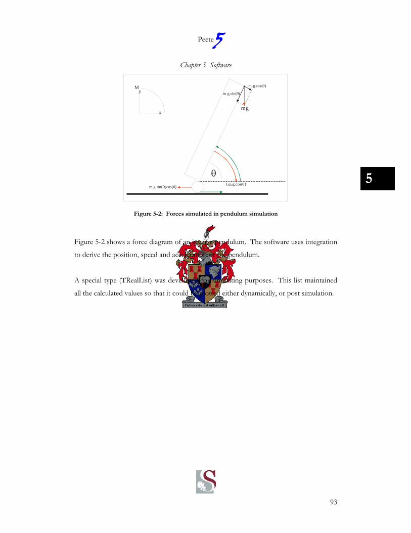
5

Peete

Chapter 5 Software

93

5θ

mg

m.g.sin( )cos( )θ θ

m.g.sin( )θ

m.g.cos( )θ

x

yM

l.m.g.cos( )θ

Figure 5-2: Forces simulated in pendulum simulation

Figure 5-2 shows a force diagram of an inverse pendulum. The software uses integration

to derive the position, speed and acceleration of the pendulum.

A special type (TRealList) was developed for simulating purposes. This list maintained

all the calculated values so that it could be plotted either dynamically, or post simulation.

5

Peete

Chapter 5 Software

94

5

Figure 5-3: Screen capture of pendulum simulation

Figure 5-3 shows a screen capture of the pendulum simulation program. It too uses a

MDI interface. The list box on the left hand side shows all the variables that have been

created for the simulation. Any one of these variables can be dragged and dropped on

any one of the charts. The user can create as many charts as the PC memory allows.

Features of the pendulum simulation program include:

• Representative simulation of real-world modals.

• Multiple graphing capabilities.

• Visual display of the actual motion of the pendulum.

• Kalman filter testing.

• Exporting of data for further processing.

5

Peete

Chapter 5 Software

95

5

5.2.3 Ultrasonic Simulation software

The ultrasonic simulation software was used to simulate and test the ultrasonic

algorithms. The use of this software was explained in 3.4.4 and a screen capture of the

software can be seen in Figure 3-25.

The features of this software included:

• Complete simulation of transmit and receive algorithms.

• Simulation of electronic hardware.

• Run-time adjustable simulation parameters.

• Data exporting for post-analysis in other programs.

5.3 Matlab software

A lot of the early simulation work was done in Matlab11 but was eventually done in

Delphi to simplify the process of porting the final code to the embedded C.

Matlab was mostly used for post processing of data. All of the FFT analysis shown in

Chapter 3 was done in Matlab. Matlab was also used for:

• Filter design (see APPENDIX A)

• Initial testing of transmit and receive algorithms.

• Testing of matrix mathematics developed for position calculation.

5.4 C software

All of the embedded software was developed in C. There are four different projects that

were created for the embedded code:

11 Matlab software can be found in .\programming\matlab\

5

Peete

Chapter 5 Software

96

5

• Main12 was used for the application and control software running on the main

DSP.

• RX13 was used for the receive algorithms running on the second RX DSP.

• TX14 was used to the code running on the main DSP, but when the PCB is used

as a transmitter board.

• A Boot loader was developed to run on the two processors used. The boot

loader software enables the upgrading of application software through any of the

communication ports. It can be used to upgrade any of the robot’s software

through the RF interface at any time.

Figure 5-4: Partitioning of C software

The first three projects are sub divided in to the following sections:

• Application Layer (APP)

• Peripherals

• Hardware Abstraction Layer (HAL)

12 .\motherboard\programming\c\main\ 13 .\motherboard\programming\main\RX\ 14 .\motherboard\programming\main\TX\

5

Peete

Chapter 5 Software

97

5

5.4.1 Application Layer

The APP layer is the part of the software that is very similar to normal PC software.

This software is completely independent of the platform that it is running on. This will

include software like the position calculation routines. These routines could have been

developed on a PC and then used in the embedded software. It simply takes distance

measurements and calculates the robots position. It does not know how those

measurements were made and it cannot control it directly.

This layer of software can be written and changed by anybody that is familiar with the C

language. It is physically also separated in to different files to make it easy to distinguish

from the other layers of software.

5.4.2 Peripherals

The peripheral layer of software is completely device or platform dependant. This

software provides the interface between the application layer and the outside world

(analogue sensing, flashing of an LED, etc.).

The peripheral software includes all the communication drivers, initialization code, etc.

It was written in such a way that it could be easily replaced by other drivers should the

software ever need to run on a different platform. This ensures that the application layer

software does not need changing should the need arise to change the processor.

5.4.3 Hardware Abstraction Layer

The line between the HAL layer and the peripheral layer is often very blurred. The idea

of this layer of software is to control hardware that is external to the processor. External

hardware is almost always controlled from peripherals and in some cases it would over

complicate the software if the two were split up.

An example of HAL code is the motor drivers. The stepper motor driver IC’s are

controlled by using three of the DSP’s peripherals (PWM, GPIO and SPI). In this case,

5

Peete

Chapter 5 Software

98

5

it is easier to group everything together in to a single layer. The peripherals used in such

a case do not fall under the peripheral layer.

5.5 Conclusion

Good software will comply with the following basic rules:

• Has to be stable and reliable.

• Has to be maintainable.

• Has to be easy to read and understand.

• Has to be user friendly.

The software (both PC and embedded) written for Peete5 complies with all of these

basic rules.

The software is very stable. Throughout the development of this project, there has not

been a single crash of the PC or the embedded software. Re-try mechanisms in the

communication protocol assures that commands are sent and received correctly even

with a very bad communication link. Error and warning messages will give feedback to

the user whenever there are detectable failures.

The code has been structured in such a way that different parts of the code can be

improved on with very little to no knowledge of the parts that it interacts with. This

means that the code can be maintained and improved very easily. The OOP style of the

PC software takes this method of programming even further.

Extensive commenting (see APPENDIX D) and a fixed coding standard throughout all

the code improve the readability of the software. Complex blocks of code have good

explanations prior and during the code. Assembler code for example has an explanation

on almost every line and aims at teaching this language even to someone who is not

familiar with it.

5

Peete

Chapter 5 Software

99

5

A plug and play (or start-up and use) approach was used when developing software to

ensure that even a novice programmer and user should be able to use and understand the

software.

Chapter 6 Mechanical Design

6.1 Introduction

The mechanical design of the Peete5 is very

simple. This was one of the main design goals

when designing the robot’s mechanical housing.

The second design goal was to mount and house

the electronics used.

The simplicity of the final design means that this

chapter will focus on the design process

followed rather than the final design itself.

The chapter will start of by stating the design goals for the mechanical design of Peete5.

Most of this chapter will show the different designs that were made for Peete5. It will

point out the advantages as well as the disadvantages of the different configurations and

will end off by showing the final design and why it was chosen.

5

Peete


101

6

6.2 Design Goals

Peete5 was mainly an electronic and software design. Although the mechanical design

was always an after-thought, it did have a reasonable degree of importance. In order to

assure a good mechanical design, some design goals were set to lead the mechanical

design:

• Must be easy to build.

This was the first and most imported design goal. Very little time had to be spent

on assembling the robot. Since a lot of debugging would be done once it was

built, it also had to be easy to get access to the electronics. Assembling and

disassembling the robot had to be quick and easy.

• Must to be robust.

This requirement speaks for itself. The robot should be able to withstand

everyday usage (picking up, placing on desks, etc.).

• Must protect the electronics.

This requirement was two-fold. The electronics had to be protected from

handling (prevent static damage) as well as provide shielding for the two RF

sections (transceiver and video transmitter).

• Must to be light.

A heavy robot is more difficult to manoeuvre and will require stronger motors.

The stronger motors would in turn require more complicated electronics and

batteries.

• Must be small.

This requirement is actually derived from easy to build and have to be light. A

small robot requires simple tools to put it together and is lighter than a big robot

made from the same material. The robot had to be just big enough to house the

electronics and this had to be as small as possible.

5

Peete


102

6

6.3 Peete5.0

Figure 6-1: Mechanical drawing of Peete5.0

Figure 6-1 shows the first attempt at a mechanical design for Peete5. This robot is a very

basic and familiar robot design. It is a three wheeled robot. The two front wheels are

used to propel as well as steer the robot. The third back wheel would swivel and is there

only to support the robot.

These types of designs are normally done with a second support wheel. The two steering

wheels would sit in the middle of the robot with the two swivelling wheels at the front

and the back. The advantage of having a second wheel is that the robot can turn around

its own centre making it easy to manoeuvre.

This design used DC motors for propulsion for Peete5.

5

Peete


103

6

Figure 6-2: Peete5.0 motor assembly

Figure 6-2 shows the motor assembly used for Peete5.0. The DC motor (shown top

right) assembled in to a bracket (shown in blue) that was attached to a sheet-metal

housing. A long axel would attach the motor to the wheel. The outer sheet metal part

provided support for the long axel.

A wheel counter (shown in purple) was attached to the axel to give feedback on the

current position of the wheels. The idea was to design a complete motor assembly unit

with a PCB at the bottom that contained the electronics needed to drive the DC motor

as well as get the feedback from the wheel counter.

6.3.1 Advantages

This robot would have been fairly simple to build and assemble. The separate wheel

assemblies would also make the final electronic design simpler. The big platform of the

robot would mean that extra peripherals (an arm perhaps) could be attached to the back

of the robot.

5

Peete


104

6

6.3.2 Disadvantages

This design had several disadvantages. The box design would make it easy to build but it

was very unstable. Note the large areas in the back corners. The slightest push in the

back corners would lift up one of the front wheels. The back wheel was difficult to

implement and required its own bracket to be attached to the body of the robot.

Although the design looks simple, it would have been relatively difficult to make.

Almost all the sheet metal parts require some machining.

The sheet metal parts required for this robot was bigger than it had to be. The corners at

the back were taking up unnecessary space. This design was eventually scrapped before

the head could be finished.

6.4 Peete5.1


5

Peete


105

6

Figure 6-1 shows the mechanical drawing of Peete5.1. This design attempted to solve

the following disadvantages of the previous design:

• The corners of the robot were taken away making it more stable.

• The number of metalwork required for the outside of the robot was reduced.

This design used the PCB (shown in green) as the base for the mechanical design. The

motor assemblies of the previous design was kept and could be made together would the

main PCB. A spring mechanism was added to give some flexibility to the robot making

it more robust.

The problem of attaching the back wheel is solved relatively easy by attaching a bracket

(shown in blue) to the back of the PCB. The bracket holds the back wheel in place.

This robot would have two axes of movement on its head. The two servo motors were

attached to one another and the PCB with the use of simple bent brackets. This enabled

the robot to look up and down and left and right.

6.4.1 Advantages

This robot would have been even easier to build than the previous one because it is not

enclosed in anything. The back wheel, servo motors and motor assemblies would simply

attach to the PCB. The two degrees of freedom on the head would have been a nice to

have.

The body of the robot forms a triangle making it stable and less susceptible to tip over.

6.4.2 Disadvantages

This robot required too many special brackets. The brackets were designed from sheet

metal parts.

5

Peete


106

6

Figure 6-4: Servo bracket – Unfolded

Figure 6-5: Servo bracket - Folded

Figure 6-4 and Figure 6-5 shows the design of the servo bracket. The bracket would be

made but cutting out a peace of sheet metal and drilling the required holes. The metal is

then bent on the dotted lines to get the final bracket. Although these parts are relatively

easy to make, this design would require six separate parts. This would have been costly

and time-consuming to make.

This robot still had a third wheel. This meant that it could not turn on its own axes.

The mechanical design was completed but it was decided to make something that would

be simpler to manufacture.

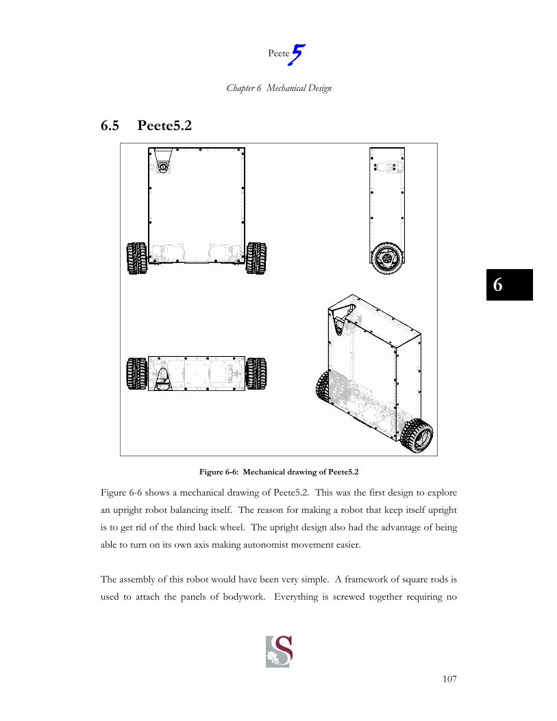
5

Peete


107

6

6.5 Peete5.2


Figure 6-6 shows a mechanical drawing of Peete5.2. This was the first design to explore

an upright robot balancing itself. The reason for making a robot that keep itself upright

is to get rid of the third back wheel. The upright design also had the advantage of being

able to turn on its own axis making autonomist movement easier.

The assembly of this robot would have been very simple. A framework of square rods is

used to attach the panels of bodywork. Everything is screwed together requiring no

5

Peete


108

6

bonding, bending, welding, etc. The complete assembly could be made with a single

screw driver.

6.5.1 Advantages

The main advantage of this design is easy of assembly. The design is also very robust

because all the electronics can be shielded inside the box. Getting to the electronics

would require the removal of the front or back panel without compromising the

mechanical integrity of the box.

6.5.2 Disadvantages

This design was easier to assemble than the previous two designs but still had some

disadvantages. One that may not be so obvious at first is the breadth of the robot.

Keeping the robot upright was seen as a nice to have but it should have been possible

not to implement it if the design ran out of time. If the robot could be put on its back

with a small wheel, then it would still be able to meet the original design intent al be it

not so graceful. This design made it impossible because the two side wheels would not

reach the ground if the robot was placed on it’s back (see side view in Figure 6-6).

5

Peete


109

6

6.6 Final solution

Figure 6-7: Mechanical drawing of final design

The final design used for Peete5 is shown in Figure 6-7. Note that this design contains

more information like the PCB, battery etc.

This design continued on the upright robot shown in the previous design. It solved the

shortcomings of the previous design by reducing the size of the robot. The breadth of

the robot is much less giving some ground clearance should the robot be placed on its

back.

5

Peete


110

6

The amount of material needed was reduced quite substantially. This was done by using

smaller motors (the DC motors were dropped because of the simplicity in position

control of stepper motors – see section 4.7) and moving the head assembly to the outside

of the box. The framework with attached panels was also replaced by a thicker base and

top plate to which the other panels were attached. Some extra re-enforcements were

made by using triangular peaces to attach the front at back plates to the sides. This

turned out to be unnecessary since the box was strong enough on its own.

6.6.1 Advantages

This robot was simple to assemble (again using only a screw driver), screened the RF

parts and protected the electronics. It is light, small and very robust. The robot could

also be operated standing up, or lying on its back (even the camera can swivel to the top

of the robot looking forward should it lay on its back).

All the design goals set for the mechanical design was met by this design.

5

Peete


111

6

Figure 6-8: View of Peete5 without front panel

The picture shown in Figure 6-8 shows the final assembly of Peete5. The front panel has

been removed to clearly show the inside of the robot.

The complete set of assembly drawings of Peete5 can be found in APPENDIX E.

6.6.2 Disadvantages

Some features were given away in order to meet the original design goals. The two

designs before this one had a spring system on the wheel assemblies. This would have

smoothed the ride a bit for the electronics and the camera. Especially the camera view

would be a lot shakier on this design.

5

Peete


112

6

6.7 Conclusion

The final mechanical design meets all the requirements set out in the beginning of this

chapter.

Figure 6-9: Photograph of Peete5

Although the final design (Figure 6-9) may look simple, this is exactly what is was

designed for. The different designs shown in this chapter showed how good thinking

and development prior to manufacturing can be used to come up with a mechanical

design that not only meets, but exceeds all the design expectations.

Chapter 7 Keeping Peete5 upright

7.1 Introduction

Keeping Peete5 upright is a design constraint that has

been placed on the software and electronics due to the

mechanical solution described in the previous chapter. It

is not one of the requirements of this project and has

been done purely to demonstrate how a good mechanical

design can be obtained through the use of simple and

low cost electronic and software design.

The DSP used on the motherboard is a powerful number

crunching machine and is ideal for doing the mathematics required for keeping Peete5

upright. It contained Analogue to Digital converters already and the only extra

requirement was inertial reference sensors.

This chapter will explain how the inertial sensors were used. It will explain how they

were calibrated and how a Kalman filter can be used to get the best possible

measurements from the sensors.

5

Peete


114

7

7.2 Sensor calibration

Both reference sensors (Inclinometer and Gyro) were calibrated to compensate for slight

differences in the manufacturing processes of the sensors. The values calculated during

calibration were:

• Scale factor.

• Offset.

The scale factor of the sensor is the value that when multiplied with the measured ADC

value will give a value in radians (inclinometer) or radians/second (gyro).

According to the inclinometer datasheet, the 0g offset voltage can differ by as much as

625 mV while the sensitivity can change by as much as 25 mV depending on the supply

voltage. Using the typical values from the datasheet can result in errors of a couple of

degrees when measuring the orientation of the robot. A simple calibration procedure

was used to calibrate the sensor. These values do not change over time and only a single

calibration is needed.

Note: The offset and scale factors will also change over temperature. These changes can be neglected since

Peete5 is expected to only operate at room temperature.

7.2.1 Inclinometer

The Peete5 PCB was placed on a flat surface and connected to a PC. The RAW ADC

values were measured using the “Module Testing”15 program. A protractor was used to

measure the angle of the PCB relative to the flat surface.

15 module_testing.exe

5

Peete


115

7

0 200 400 600 800 1000 1200 1400 1600 1800 20001380

1400

1420

1440

1460

1480

1500

1520

1540

1560Inclinometer Calibration

Time

RA

W A

DC

val

ue

Figure 7-1: RAW ADC values for inclinometer calibration

Figure 7-1 shows the measurements that were made as the PCB was tilted from 0° up to

90° in 15° steps. The same measurement was also done from 0° to -90°. The value

measured when the robot was standing at 0° is the offset of the inclinometer. Note how

the curve followed a sine wave and not a straight line. This is because the inclinometer is

measuring the amplitude of a vector down to earth relative to its own orientation.

Measurementvector ( )u

Gravity ( )g

Measurementvector ( )u

Gravity ( )g

Measured value (v)

θ

a) b) a) Inclinometer at 0°. b) Inclinometer at 45°.

Figure 7-2: Measuring g with an inclinometer

Figure 7-1shows an example of two measurements. The first is at 0° and the measured

value (v) is zero g. In the second example the angle is 45°. Here the measured value (v)

5

Peete


116

7

will be 21 of g. The fact that the measurement made in Figure 7-1 is a vector

measurement must be taken in to account when calibrating the sensor.

Angle [deg] g ADC value ADC - offset Scale factor

90 1 15464 1424 7.0224719101E-0475 0.96592583 15408 1368 7.0608613033E-0460 0.8660254 15254 1214 7.1336524200E-0445 0.70710678 15016 976 7.2449465286E-0430 0.5 14704 664 7.5301204819E-0415 0.25881905 14352 312 8.2954822148E-040 0 14040 0

-15 -0.25881905 13692 -348 7.4373288823E-04-30 -0.5 13326 -714 7.0028011204E-04-45 -0.70710678 13032 -1008 7.0149482261E-04-60 -0.8660254 12806 -1234 7.0180340663E-04-75 -0.96592583 12656 -1384 6.9792328489E-04-90 -1 12612 -1428 7.0028011204E-04

7.2285567603E-04

Table 7-1: Calculating inclinometer offset and scale factor

Table 7-1 shows how the inclinometer offset and scale factor were calculated. The Angle

is the angle at which the PCB was tilted when the ADC measurement was made. The g

value is sin(angle) and is the value that the inclinometer would have been measuring.

The scale factor is the value that will convert the measured ADC voltage to the measured

g value. The average off all the scale factors was used to obtain the final value.

One g is equal to 90°. Multiplying the scale factor by π/2 then will convert raw ADC

values to radians.

Note: The standard measuring unit used when writing software was radians.

7.2.2 Gyro

The rate gyro also needed calibration in order to convert the raw ADC value to a rate in

rad/sec. The rate gyro was attached to one of the stepper motors of Peete5. The

functions for controlling the stepper motors are very accurate and a very accurate angular

speed command can be sent to the stepper motors. This angular speed can then be used

to calculate the scale factor of the sensor. The same process was followed as that used

5

Peete


117

7

for the inclinometer calibration, the only difference being that stepper motor speed was

used, and not the angle of the board.

The offset value of the rate gyro can not be calibrated out. This is because of the fact

that all rate gyros have an inherent drift in its offset value. This drift has to be calculated

by using the inclinometer output. A Kalman filter is needed for this and is explained

next.

7.3 Kalman filter

The equations for a Continuous-Discrete Kalman Filter are given in [4] as:

The system model is given by:

GwBuAxx ++=&

7-1

The measurement model is given by:

kkk vHxz +=

7-2

Initialization:

00 )0(ˆ,)0( xxPP ==

7-3

The time update between measurements can be done by: TT GQGPAAPP ++=&

BuxAx += ˆ&̂

7-4

5

Peete


118

7

And the measurement update at times tk is calculated with: 1])([)( −−− += RHtHPHtPK T

kT

kk

)ˆ(ˆˆ)()()(

−−

−

−+=

−=

kkkk

kkk

xHzKxx

tPHKItP

7-5

The goal behind all these equations was to calculate the Kalman gain (Kk) which is then

used to calculated the estimated angle and gyro drift (in the vector xk). The output of the

gyro cannot be used unless its drift can be estimated. The drift will be relatively slow

(less than 1 Hz) and a Kalman filter can be used to estimate this value. It can then be

subtracted from the output of the sensor to get the rate of change in rad/sec. The value

measured by the inclinometer can be used to calculate this drift dynamically.

The two measurements made by the sensors are the angle of the inclinometer (θI) and

the rate of change of the angle (ωg). The two outputs needed from the Kalman filter will

be the true angle (θ) and the drift of the gyro (Bg). The system model (equation 7-1) can

be described by the following equations:

The rate of change of the angle is equal to the measurement made by the gyro (ωg) minus

the bias of the gyro (Bg):

gg B−= ωθ&

7-6

The bias of the gyro is slow can be seen as constant, i.e. its derivative is zero:

0=gB&

7-7

The system equation can be written in terms of Bg and θ:

5

Peete


119

7

⎥⎦

⎤⎢⎣

⎡=

gBx

θ

7-8

Taking the derivative yields:

ggg BB

x ωθθ

⎥⎦

⎤⎢⎣

⎡+⎥

⎦

⎤⎢⎣

⎡⎥⎦

⎤⎢⎣

⎡ −=

⎥⎥⎦

⎤

⎢⎢⎣

⎡=

01

0010

&

&&

7-9

Equation 7-9 is in the same form as the system model specified in equation 7-1. This is

the system model used for the Kalman filter in Peete5.

The next step is to specify the measurement modal that specifies the nature of the

measurements made. In this case the measurement model is simply the value measured

by the inclinometer since it is the only absolute measurement that can be made. The

measurement model is given by equation 7-10.

[ ] ⎥⎦

⎤⎢⎣

⎡==

gIk B

zθ

θ 01

7-10

The system requires initial values. The initial value of the estimated angle was taken as

the first inclinometer measurement (θI) and the initial gyro drift is taken as 0.

Finally, the estimated angle and drift can be calculated with:

)ˆ(ˆˆ

ˆˆ

−

−

−+⎥⎥⎦

⎤

⎢⎢⎣

⎡=

⎥⎥⎦

⎤

⎢⎢⎣

⎡kkk

kgkg

xHzKBBθθ

7-11

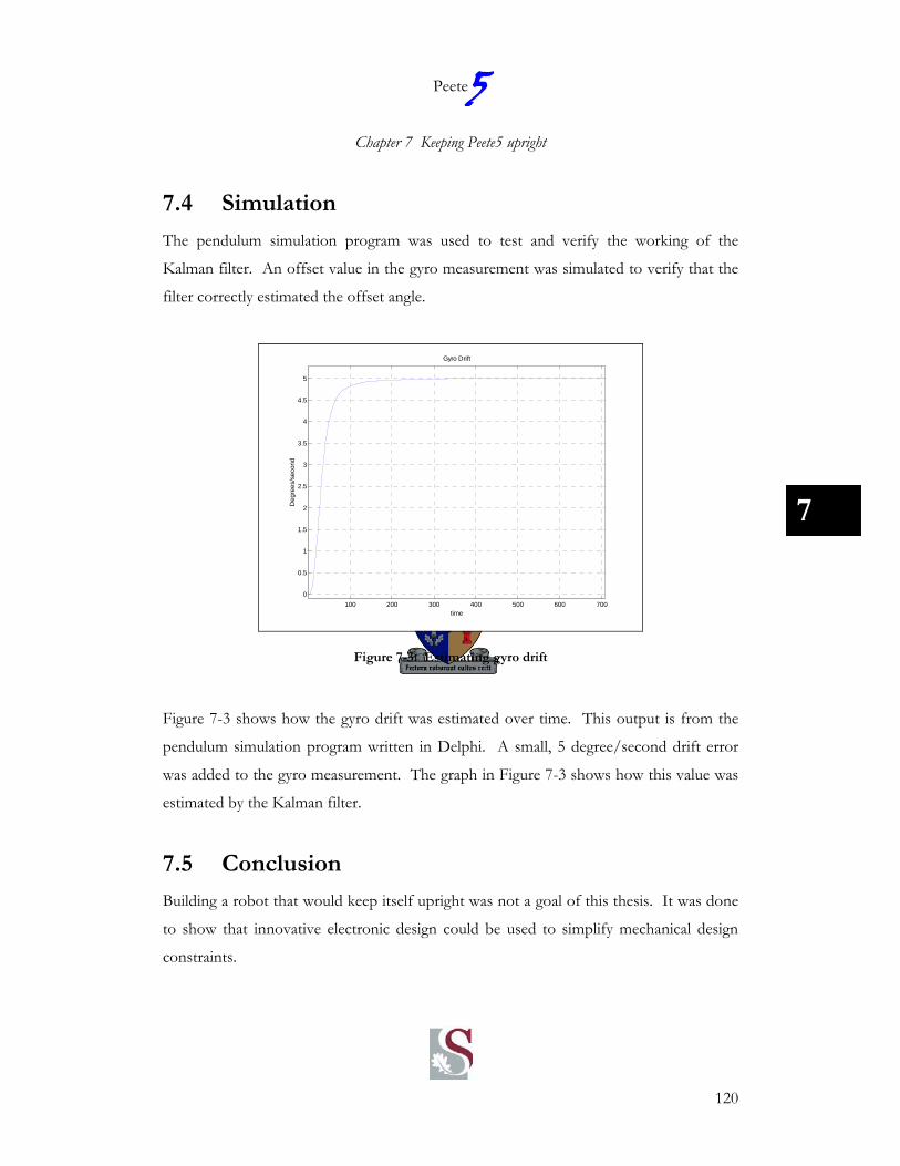
5

Peete


120

7

7.4 Simulation

The pendulum simulation program was used to test and verify the working of the

Kalman filter. An offset value in the gyro measurement was simulated to verify that the

filter correctly estimated the offset angle.

100 200 300 400 500 600 7000

0.5

1

1.5

2

2.5

3

3.5

4

4.5

5

time

Deg

rees

/sec

ond

Gyro Drift

Figure 7-3: Estimating gyro drift

Figure 7-3 shows how the gyro drift was estimated over time. This output is from the

pendulum simulation program written in Delphi. A small, 5 degree/second drift error

was added to the gyro measurement. The graph in Figure 7-3 shows how this value was

estimated by the Kalman filter.

7.5 Conclusion

Building a robot that would keep itself upright was not a goal of this thesis. It was done

to show that innovative electronic design could be used to simplify mechanical design

constraints.

5

Peete


121

7

The Kalman filter was implemented successfully. This is the first step before control

algorithms can be developed for keeping the robot upright.

A simulation program was developed successfully and showed that the dynamics of the

robot as well as the sensor readings and Kalman filter could be accurately simulated.

A control algorithm was developed and tested. It did manage to keep the robot upright

on its own and it could also withstand small step responses. The time available for

working on the control logic was very limited and a stable system could not be developed

in time. The level of success obtained in such a short time however did show that it will

be possible to keep the robot upright and it is seen as a testament to good solid

electronic design and software development. Peete5 will be an excellent test bench for

control logic development. The ease of use and the quality of the sensors make it a

stable stepping stone for future development.

122

Chapter 8 Conclusion and suggestions

8.1 Conclusion

8.1.1 Position control

Robots are slowly starting to play a bigger and bigger role in human society. If

Hollywood writers had their say, there would be a robot in every house already. Robots

are slowly starting to change from remote controlled toys to more sophisticated

autonomous systems that can be left alone to perform a specific task. Universities and

companies all over the world host competitions to develop the technologies further and

today it is possible to buy robot vacuum cleaners and lawn mowers.

One of the biggest dampers on autonomous robots today is position control. Robots

need to know where they are and where they are going. Numerous systems exist to

attempt and solve this problem. Almost all of them use some form of artificial landmark

recognition where distance sensors are used to measure the distance to a wall, table or

other obstacle. These systems have a major disadvantage in that it cannot know whether

or not something is suppose to be there. Take a robot vacuum cleaner for example. It

would navigate through a room by measuring the distance to four walls. It will generate

a mental map of what the room looks like, or it may be programmed with a map. If a

table is placed next to one of the walls then the robot would not know if it is its sensor

that is damaged or if something was placed next to a wall. It is also not possible to

calculate its exact position any more since the wall was the reference for the position

calculation.

The main design goal of Peete5 was to solve this problem by developing a system that

would use absolute positioning. Peete5 solved this problem in a simple, reliable and

extremely cost effective way. This is the first time that an ultrasonic system and RF

communication link was used to calculate the position of an object. The system made it

possible for a robot to be switched on any where in a room and it would immediately

know where it is. This is a major improvement on previous systems. If the robot

5

Peete


123

8

vacuum cleaner were to be equipped with such a system, it would be possible to navigate

its way through a room in its usual manner with the added advantage of knowing where

it is regardless of obstacles changing in its environment. Where it was previously almost

impossible to navigate back to its base station, it would now be a simple task.

Although the system is small and easy to install in a house, it is doubtful that someone

would go through the trouble when they need a vacuum cleaner. This system may

however be perfect for factories and businesses. Many manufacturing companies use

robots to carry stock and equipment from one place to another. They may use solutions

such as lines painted on the ground for the robots to follow. These systems have the

obvious disadvantage that if the line is broken or an obstacle covers the line, the system

will fail. The ultrasonic positioning system offers a very low cost solution for robot

navigation without such problems.

8.1.2 Electronic and software design

The biggest advantage of the electronic and software design in Peete5 is its stability.

Good electronic practices were followed when designing the electronic hardware and the

software. The small PCB and the fact that almost all the components are surface mount

make the PCB very robust. It has been dropped accidentally more than once and it

never needed repair. This makes the robot the perfect test bench for future development

and design. It can also be used as an example to show good industry practices today.

Possibly the second biggest advantage of the software and electronics is its ease of use.

The robot can be de-bugged, programmed and controlled with the robot switched on

and a transmitter board plugged in to a PC’s USB connector. No power supplies,

oscilloscopes or other hardware is needed. This makes it very easy and quick to develop

and test new software and it is for this reason that Peete5 is such a good test bench.

Extra communication interfaces (an SCI port) are available on headers on the PCB and

can also be used in future development should extra hardware be required.

5

Peete


124

8

The electronic circuits were designed using industry standards. This means that a

complete set of documentation is available for the manufacturing of the robot should it

ever be required. From the Gerber files for PCB manufacturing down to the parts lists

for the components.

The electronic and software designs exceed the requirements and goals set out for this

project. The robustness, ease of use, expandability and features are testament to this.

8.1.3 Mechanical Design

The simplicity of the mechanical design was explained in Chapter 6. It is this very

simplicity that makes it such a good solution. The whole of Peete5 can be disassembled

with a single screw driver. This makes it very easy to work on and maintain. The fact

that everything is securely connected to the mechanical housing makes the robot very

robust. Peete5 can easily take the odd bump or knock.

The mechanical design was not only relatively simple but also inexpensive to

manufacture. With all the design documentation available, it would be possible to easily

build another robot should it be required. The reproducibility of the robot (mechanically

and electronically) is in itself proof that the designs are very stable and mature.

Brilliant electronics and software is often let down by bad mechanical design when it

comes to robots. This was not the case with Peete5. The fact that an effort was made in

designing the hardware meant that it does not only serve a purpose, it is also good to

look at. Although no mechanical design goals were required, the internal goals

mentioned in Chapter 6 were all exceeded.

5

Peete


125

8

8.2 Suggestions

There can only be no suggestions to a finished design if no lessons were learned in the

process. This is not the case with this thesis. Many lessons were learned. Many of them

were fortunately learned in the early stages and could be incorporated in to the final

design. Some however could only been seen once the design were finished.

8.2.1 Simulation

Probably one of the most valuable design tools is simulation. It may be argued that some

systems are too complex to simulate and that it is not worth the trouble. This is not the

case. Simulation methods exist even for the robots that recently explored the surface of

Mars. More complex systems have a greater requirement for a decent simulation.

The advantage of using simulations is that small deviations can be quickly pointed out

which are more often than not the source for major problems later on. One good

example of this is the correlation algorithm used in assembler. It seemed to be working

the first time when compared to the simulation software developed for the PC. It did

however show a slight deviation now and again. It turned out that the number of

iterations used was incorrect and although it showed only sight differences when working

with no noise, it did not work at all with the addition of noise.

8.2.2 Electronic design

Careful investigation of the schematics will show a lot of zero ohm resistors and Space

Provision Only (SPO) components. These components are used as place holders. The

manufacturing of a PCB is time consuming and expensive. These extra components on

the board come at no extra cost. They are placed in case they may be needed.

Although there are some extra unpopulated components on the board, there could have

been more. The main DSP used has plenty of IO pins, ADC ports, PWM outputs and

many other extra peripherals that are not used. These should have been brought out on

5

Peete


126

8

a header of some kind, or even a prototype section on the PCB. Extra active filters could

also be added to the PCB that would have made the addition of more sensors a

possibility. This header should also include power outputs (the regulated 3.3V and 5V as

well as the unregulated 20V) so that additional boards could be made as plug-in additions

to the robot.

8.2.3 Ultrasonic positioning

Although the solution is relatively inexpensive, it does require a PCB with a DSP and

transceiver for every ultrasonic transmitter. The costs can be reduced considerably if a

single PCB could drive more than one ultrasonic transducer. The sensors could be

placed around a room and be connected to a single PCB per room.

Although the system has been proven to work, it is not without problems. Multi-path is

probably the biggest source of errors in position calculation. The GPS system suffered

the same problem but it can be corrected when using extra mathematical solutions.

Adopting the same solutions and using more than three sensors in a small area may

overcome this problem all together and even lead to more accurate position fixes.

Something that may be explored with the current hardware is working without the RF

link. The transmission of the Barker code is nothing else than sending data over a

carrier. It may be possible to send longer sequences of code that contain the actual data

needed for the position fix. The use of spread spectrum technology may even make it

possible for more than one transmitter to transmit simultaneously. This may lead to

more accurate and quicker position fixes.

127

REFERENCES

[1] Freescale Semiconductors, DSP Datasheet MC56F8346; Revision 3.0; October

2003

[2] Donald A. Neamen, “Electronic Circuit Analysis and Design”; University of New

Mexico

[3] J. Borenstein, “Where Am I? Sensors and Methods for Mobile Robot Positioning”;

University of Michigan; April 1996

[4] Frank L. Lewis, “Optimal Estimation with an introduction to Stochastic control theory”,

Wiley-Interscience publications

[5] Bosch Controller Area Network Version 2.0, Revision 3

[6] Freescale Semiconductors, MC56F8300 Peripheral User Manual; Rev 2.0; October

2003

[7] Motorola Semiconductor Application note, AN1798 – CAN Bit timing

requirements

[8] Universal Serial Bus specification, Revision 1.1; September 23, 1998

[9] Universal Serial Bus specification, Revision 2.0; April 27, 2000

[10] Raymond A. Serway, “Physics for scientists and engineers with Modern Physics”; Fourth

Edition; Saunders College Publishing; 1996

[11] Murata Manufacturing, Catalog number P19E-6; Piezoelectric Ceramic Sensors.

[12] Ziemer,Nyquist therom, page 90 – “Principles of Communications”; Tranter; Fourth

Edition; 1995.

[13] Freescale Semiconductors, DSP56F800E Reference Manual; Revision 2.0;

12/2001.

[14] Freescale Semiconductors, MC56F8300 Peripheral User Manual; Revision 2.0;

12/2001.

128

APPENDIX A : IIR FILTER IMPLEMENTATION IN DELPHI AND C

This section will explain the implementation of an IIR filter in the MC56F80xxE family

of DSP’s from Freescale. It will show how Matlab can be used to design the filter and

how Matlab and Delphi can be used to verify the correct implementation of the filter.

It uses a second order IIR implementation. The examples can be expanded to first order

IIR filters. Second order IIR filters uses less memory (RAM and ROM) and are less

susceptible to quantization noise. The draw-back is that they cannot handle filters with a

low resolution (typically where the cut off frequency is less than 10 times the sampling

frequency). First order IIR filters uses more RAM and ROM but can handle IIR filters

with a lower resolution.

N>1

Use Matlab to calculate the filter coefficients: Fs = 200e3; % sampling frequency.

Wn = [40e3]*2/Fs; % specify filter parameters.

[b,a] = butter(5,Wn);

b = b.*32767; % Convert to Q15.1.

a = a.*32767; % Convert to Q15.1.

NOTE: The filter must be designed in such a way that the filter coefficients are all smaller than 1!! A filter

with a stop band smaller than 10% of the sampling rate normally results in coefficients larger than 1.

The following filter equations are used:

∑ =+−−=

N

k k nxknwanw1

)()()(

∑ =−=

N

k k knwbny0

)()(

Note “N” in the summation (N = the order of the filter, not the number of coefficients).

The following declarations must be done in C: // IIR FILTER 0: --------------------------

#define IIR0_N 5

extern sint16 iir0_w_values[IIR0_N];

sint16* iir0_w_index;

const sint16 iir0_ba[(IIR0_N+1)*2] = {

3594, // b[1]

129

32286, // -a[1]

7189, // b[2]

-31910, // -a[2]

7189, // b[3]

12660, // -a[3]

3594, // b[4]

-3643, // -a[4]

719, // b[5]

369, // -a[5]

719, // b[0]

-32767 }; // -a[0]

Note the order of a and b and also the fact that a is negated (this is to use mac where only accumulations

are done).

The extern iir0_w_values is the circular buffer to store w(n) and is declared in an

assembler file as:

global Fiir0_w_values

Fiir0_w_values bsm 6

The following code will then implement and test the filter:

void test_filter(sint16 value_in)

{

sint16 value_out;

// Note: value passed in Y0.

asm

{

moveu.w #IIR0_N, M01 // Use modula adressing.

moveu.w #iir0_ba, R3 // Start at b[1].

moveu.w iir0_w_index, R0 // Load index in to w.

move.w Y0,A // w0 = x0.

clr B X:(R0)+,Y0 X:(R3)+,X0 // y0 = 0;

// load w[0] and load b[1] point to a[1].

do #IIR0_N,__end_do

macr Y0,X0, B X:(R3)+,X0 // y0 += b[i]*w[i] |

// load a[i]

macr Y0,X0, A X:(R0)+,Y0 X:(R3)+,X0 // w0 += a[i]*w[i] |

// load w[i] and b[i]

__end_do:

move.w X:(R0)-, Y0 // This is just to decrement R0.

130

macr A1,X0, B // y[0] = y[0] + w[0]*b[0].

move.w A1, X:(R0)

move.w R0, iir0_w_index

move.w B1,value_out

moveu.w #0xFFFF, M01

}

printf("%i \n",value_out);

} // test_filter

The impulse response given in matlab (using impz):

0 5 10 15 20 25 30 35-0.2

-0.1

0

0.1

0.2

0.3

0.4

0.5

Now compare this output with the simulated values in Delphi and finally with that in C:

Simulation in Delphi

Simulation in Matlab

scale Matlab

normalized to Q16

Error between Delphi and

Matlab

Simulation in DSP

Error between DSP and Delphi

719 0.021939621 32771.76074 719 0 719 0

4302 0.131315765 32771.76074 4303 1 4302 0

10728 0.32741906 32771.76074 10730 2 10728 0

13847 0.422605216 32771.76074 13850 3 13847 0

8372 0.255540671 32771.76074 8375 3 8372 0

-842 -0.02567346 32771.76074 -841 1 -842 0

-4777 -0.145796607 32771.76074 -4778 -1 -4777 0

-2071 -0.06321571 32771.76074 -2072 -1 -2071 0

1512 0.04612992 32771.76074 1512 0 1512 0

131

1849 0.056418323 32771.76074 1849 0 1849 0

71 0.002161138 32771.76074 71 0 71 0

-970 -0.029605805 32771.76074 -970 0 -970 0

-501 -0.015318391 32771.76074 -502 -1 -501 0

291 0.008820873 32771.76074 289 -2 291 0

412 0.012566065 32771.76074 412 0 412 0

39 0.001188536 32771.76074 39 0 39 0

-206 -0.006288972 32771.76074 -206 0 -206 0

-120 -0.003652257 32771.76074 -120 0 -120 0

55 0.001687511 32771.76074 55 0 55 0

91 0.002799125 32771.76074 92 1 91 0

13 0.000416087 32771.76074 14 1 13 0

-43 -0.001328801 32771.76074 -44 -1 -43 0

-28 -0.000861775 32771.76074 -28 0 -28 0

10 0.000313528 32771.76074 10 0 10 0

20 0.000620048 32771.76074 20 0 20 0

4 0.00012507 32771.76074 4 0 4 0

-8 -0.000278635 32771.76074 -9 -1 -8 0

-6 -0.000201345 32771.76074 -7 -1 -6 0

1 5.58843E-05 32771.76074 2 1 1 0

4 0.000136572 32771.76074 4 0 4 0

0 3.47369E-05 32771.76074 1 1 0 0

-3 -5.79382E-05 32771.76074 -2 1 -3 0

N = 1

Use Matlab to calculate the filter coefficients: Fs = 200e3; % sampling frequency.

Wn = [10e3]*2/Fs; % specify filter parameters.

[b,a] = butter(1,Wn);

b = b.*32767; % Convert to Q15.1.

a = a.*32767; % Convert to Q15.1.

NOTE: The filter must be designed in such a way that the filter coefficients are all smaller than 1!! A filter

with a stop band smaller than 10% of the sampling rate normally results in coefficients larger than 1.

The following filter equations are used:

∑ =+−−=

N

k k nxknwanw1

)()()(

∑ =−=

N

k k knwbny0

)()(

Note “N” in the summation (N = the order of the filter, not the number of coefficients).

132

The following declerations is then done in C: // IIR FILTER 1: --------------------------

#define IIR1_N 1

const sint16 iir1_ba[(IIR1_N+1)*2] = { 23807, // -a[1]

4480, // b[1]

4480, // b[0]

-32767 }; // -a[0]

sint16 iir1_w_value;

Note the order of a and b and also the fact that a is negated (this is to use mac

where only accumulations are done).

The following code will implement and test the filter:

void test_filter2(sint16 value_in)

{

sint16 value_out;

// Note: value passed in Y0.

asm

{

moveu.w #iir1_ba,R3 // Point to a1

move.w iir1_w_value, X0 // Load w[0-1]

move.w Y0, A // w[0] = x[0]

move.w X:(R3)+,Y0 // Load a1.

macr Y0,X0,A X:(R3)+,Y0 // w[0] = w[0] + a[1]*w[0-1] ||

// load b1.

mpyr Y0,X0,B X:(R3)+,Y0 // y[0] = b[1]*[w0-1] ||

// load b0.

macr A1,Y0,B // y[0] = y[0] + b[0] * w[0].

move.w A1, iir1_w_value // Save w[0].

move.w B1, value_out

}

printf("%i \n",value_out);

} // test_filter

The impulse response given in Matlab (using impz(b,a)):

133

0 5 10 15 20 25 300

0.05

0.1

0.15

0.2

0.25

Now compare this output with the simulated values in Delphi and finally with that in C.

134

APPENDIX B : COMMUNICATION MESSAGES

1. status

This command is used to get the status of a specific module. All modules must respond

to this message regardless of the state they are in.

Packet format: Byte no. Description

0 Source address.

1 Destination address.

2 Command identifier – see Table 3-1.

3 Message CRC

Message response: Byte no. Description

0 Source address.


2 Response identifier – see Table 3-1.

3 Board state – see Table 8-1.

4-7 Warning bits.

8-11 Error bits.

12 Last error/warning.

13-16 Debug parameter.

17,18 Message CRC

a. Board states

The states that a module can be in are listed in the following table. The state can be

determined by sending the module a status command.

State Description Value

Startup The module is busy starting up and initializing. 0x01

Running The module is functioning normally. 0x02

Error The board is in the error state. 0x03

135

Software

download

The board is in the software download state. This means that

the application code is not running, but the loader code.

0x04

Table 8-1: Board states

b. Warning bits

Bit number Warning

0 C1000 calibration failed (my still work though if really lucky)

1

2

3-31 Unused.

Table 8-2: Warning bits

c. Error bits

Bit number Error

0 Data flash programming failed.

1 Data flash erasure failed.

2 Program flash programming failed.

3 Program flash erasure failed.

4 PLL not locked (it must be to program correctly).

5 CLKD invalid (must be valid to program correctly).

6 Application CRC invalid.

7 Loader CRC invalid.

8 Application size invalid.

9-31 Unused.

Table 8-3: Warning bits

2. enter_sw_download

Use this command to enter the software download state. If the application code is

running, then it must jump to the bootloader code and command it to enter the software

136

download state. No other download command shall be accepted unless the bootloader is

in the software download state.


0 Source address.



3 Message CRC


0 Source address.



3 0 – Command accepted.

1 – Command rejected.

4+5 Message CRC

3. start_sw_download

Use this command to start a new software download. The entire data flash and program

flash sections will be erased on receiving this command.


0 Source address.



3 Major part of software version.

4 Minor part of software version.

5 Release day.

6 Release month.

7 Release year.

8,9 Message CRC

137


0 Source address.





4 TX buffer size. This size will determine the size of the data packets being sent during

programming. A whole data packet shall not be larger than this value.

5+6 Message CRC

4. program_flash

Use this command to program a block of flash.


0 Source address.



3 Number of bytes to follow (N)

Specify how many data bytes will follow.

4,5,6,7 Start address.

This address is the start address (in the flash) of the block of data to follow. The most

significant bit specifies weather it is data or program flash. If the address is greater than

0x80000000 then it is data flash, and will program to data flash address 0x00000000.

8 – (N+7) The data to program (MSB,LSB).

(N+8) +

(N+9)

Message CRC


0 Source address.




138


4+5 Message CRC

5. stop_sw_download

Use this command to stop a software download that is currently in progress. If a

programming session was in progress then the CRC of the flash will be checked and

compared with the CRC sent to it by this command. The command will only be

accepted if the calculated CRC is the same as the given CRC.


0 Source address.



3,4 Flash CRC. The boot-loader should get the same value when calculating the CRC over the

flash.

5,6,7,8 Number of words that have been programmed (data + program flash)

9 New device address. The device shall use this address to compare with the destination address

of incoming messages.

10,11 Message CRC


0 Source address.



3 0 – Command accepted (CRC OK).

1 – Command rejected (CRC failed or no download was in progress).

4+5 Message CRC

6. get_raw_adc

Use this command to read the raw ADC values as sampled by the analog to digital

converter on the DSP. The values are all 16-bit values and can be interpreted as signed

or unsigned. The sign will depend on the specific application of that ADC.

139


0 Source address.



3+4 Message CRC


0 Source address.



3+4 ADC A0

5+6 ADC A1

6+7 ADC A2

… …

17+18 ADC A7

19+20 ADC B0

… …

33+34 ADC B7

35+36 Message CRC

7. send_dist_pulse

Use this command to let the transmitter send out an ultrasonic pulse. This pulse will be

the fully modulated code word for ultrasonic range finding.


0 Source address.



3+4 Message CRC

Message response:

140

Byte no. Description

0 Source address.



3+4 Message CRC

8. force_calculate_distance

This command can be used to force the main processor to attempt a distance calculation.

This command should only be used if normal distance calculation was disabled in the

source code.


0 Source address.



3 ID of TX node. The main board will send a “send_dist_pulse” command to the board with

this ID and use the response to calculate the distance from it.

4+5 Message CRC


0 Source address.



3+4 Message CRC

9. reset

This command will force the board to do a software reset.


0 Source address.


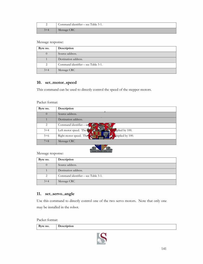
141


3+4 Message CRC


0 Source address.



3+4 Message CRC

10. set_motor_speed

This command can be used to directly control the speed of the stepper motors.


0 Source address.



3+4 Left motor speed. The speed is in radians, multiplied by 100.

5+6 Right motor speed. The speed is in radians, multiplied by 100.

7+8 Message CRC


0 Source address.



3+4 Message CRC

11. set_servo_angle

Use this command to directly control one of the two servo motors. Note that only one

may be installed in the robot.


142

0 Source address.



3+4 Servo 0 angle. This must be a value between 0 and 180 and is the servo angle in degrees

multiplied by 100.

5+6 Servo 1 angle. This must be a value between 0 and 180 and is the servo angle in degrees

multiplied by 100.

7+8 Message CRC


0 Source address.



3+4 Message CRC

12. get_last_dist_cntr

This command can be used to get the last correlation counter that was passed on from

the RX board to the Main board through the CAN interface. This counter can be used

to calculate distance.


0 Source address.



3+4 Message CRC


0 Source address.



3+4 Distance measured. This value is the last distance measured between this Main board and a RX

board. This value is distance in mm.

5+6 Second correlation counter. This counter is the counter value at the time when the highest

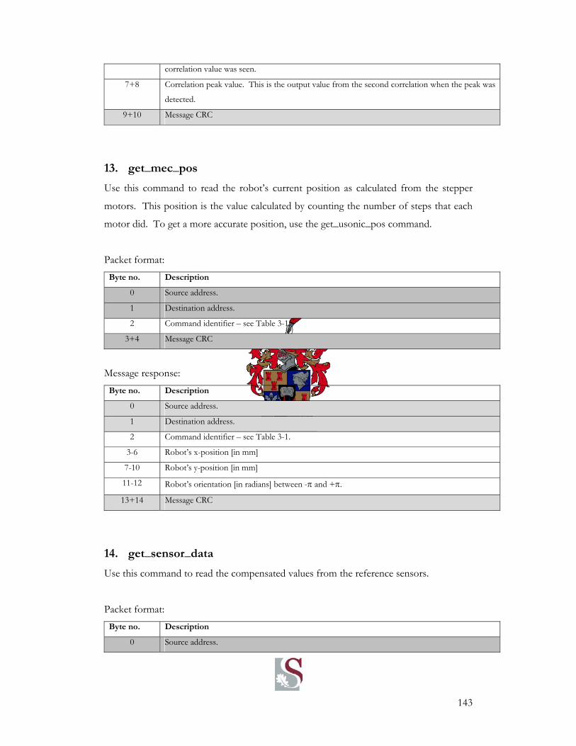
143

correlation value was seen.

7+8 Correlation peak value. This is the output value from the second correlation when the peak was

detected.

9+10 Message CRC

13. get_mec_pos

Use this command to read the robot’s current position as calculated from the stepper

motors. This position is the value calculated by counting the number of steps that each

motor did. To get a more accurate position, use the get_usonic_pos command.


0 Source address.



3+4 Message CRC


0 Source address.



3-6 Robot’s x-position [in mm]

7-10 Robot’s y-position [in mm]

11-12 Robot’s orientation [in radians] between -π and +π.

13+14 Message CRC

14. get_sensor_data

Use this command to read the compensated values from the reference sensors.


0 Source address.

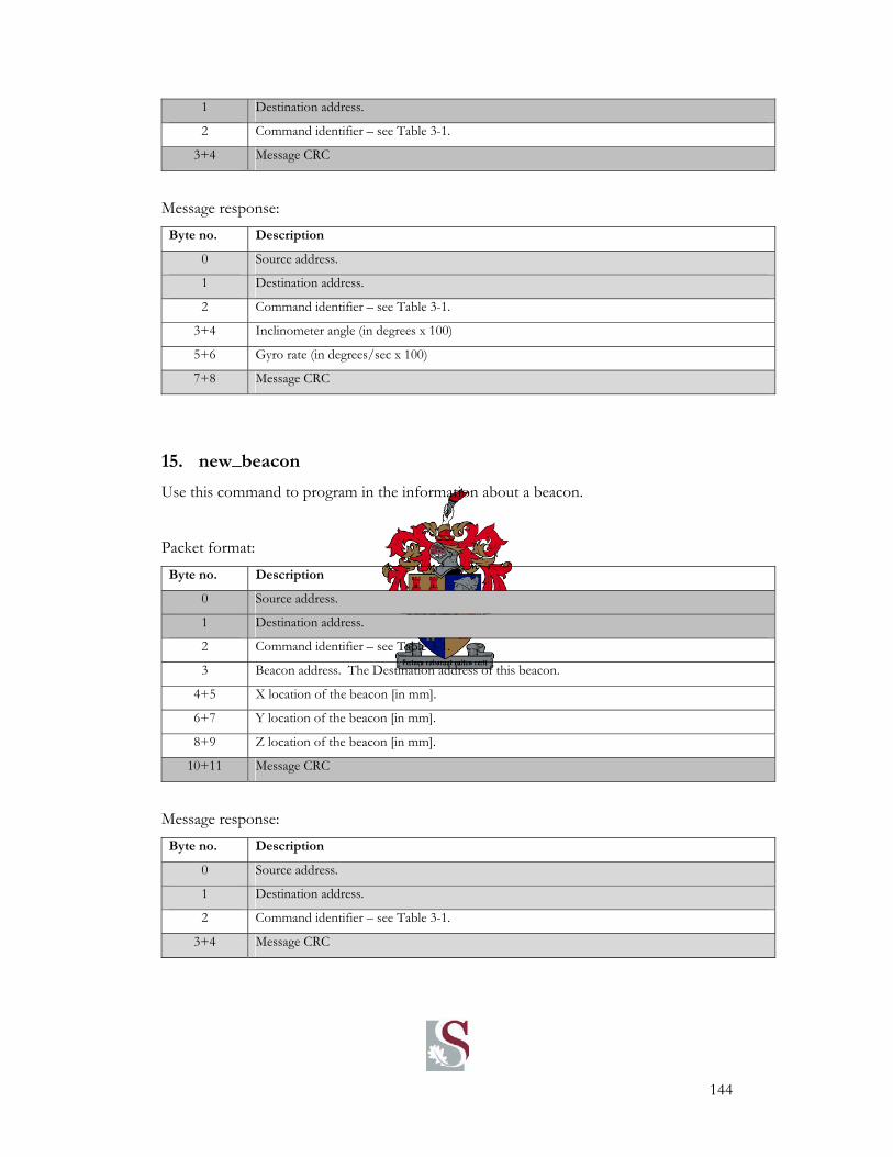
144



3+4 Message CRC


0 Source address.



3+4 Inclinometer angle (in degrees x 100)

5+6 Gyro rate (in degrees/sec x 100)

7+8 Message CRC

15. new_beacon

Use this command to program in the information about a beacon.


0 Source address.



3 Beacon address. The Destination address of this beacon.

4+5 X location of the beacon [in mm].

6+7 Y location of the beacon [in mm].

8+9 Z location of the beacon [in mm].

10+11 Message CRC


0 Source address.



3+4 Message CRC

145

16. update_position

This command can be used to force the robot to do a update on it’s position. The robot

will measure the distance to all of the programmed beacons (as if a force_calc_dist

command has been received, but to all of the beacons). It will also attempt to get a

position fix after each beacon’s information has been updated.


0 Source address.



3+4 Message CRC


0 Source address.



3+4 Message CRC

17. get_beacon_info

This command can be used to get the latest information from all of the beacons. This

will include the beacon’s position, and the distance measured to the beacon (if a distance

has been measured before).


0 Source address.



3+4 Message CRC

Message response:

146

Byte no. Description

0 Source address.



3 Number of programmed beacons (N).

4 Address of Beacon 0.

5+6 X-location of Beacon 0 [in mm].

7+8 Y-location of Beacon 0 [in mm].

9+10 Z-location of Beacon 0 [in mm].

11+12 Last distance measured to Beacon 0 [in mm]

… …

4+9*(N-1) Address of Beacon N.

5+9*(N-1) X-location of Beacon N [in mm].

7+9*(N-1) Y-location of Beacon N [in mm].

9+9*(N-1) Z-location of Beacon N [in mm].

11+9*(N-1) Last distance measured to Beacon N.

Message CRC

18. get_usonic_pos

Use this command to read the position that was calculated after an ultrasonic fix was

made.


0 Source address.



3+4 Message CRC


0 Source address.



3-6 Robot’s x-position [in mm].

147

7-10 Robot’s y-position [in mm].

11-14 Robot’s z-position [in mm].

15+16 Message CRC

148

APPENDIX C : SCHEMATICS

11

22

33

44

55

66

77

88

DD

CC

BB

AA

Title

Num

ber

Rev

isio

nS

ize

A3

Dat

e:20

04/1

1/20

She

et

of

File

:C

:\Pee

te5\

..\U

ltra

Son

ic.S

CH

DO

CD

raw

n By

:

+18V

_U+1

8V_U

Vpu

lse

Vpu

lseN

+18V

_U

0RR77

0RR74

Wil

dalk

and

er re

sist

or w

aard

es h

ier i

nsit

om d

ie s

troom

deu

r die

tran

sist

or te

bep

erk?

1kR93

10k

R97

47k

R88

4k7

R90

100n

C10

7

4k7

R91

47k

R89

MA

40E

7R/S

X1

BC

817-

40Q

2

BC

817-

40Q

3

BC

807-

40Q

4

10n

C12

0

Ferri

teL1

3Vi

n+1

8V_U

10u;

50V

C12

3

+3V

3

3k9

R92

1nC10

6

1kR94

US

_out

100n

C11

9

+3V

3

2 31

114

Op.

am

p.U

14A

10k

R10

1

10k

R10

2

10k

R98

+3V

3

+3V

3

100n

C11

5

1kR95

13 1214

114O

p. a

mp.

U14

D

10k

R99

+3V

3

100n

C11

7

33k

R70

9 108

114

Op.

am

p.U

14C

33k

R71

+3V

3

100n

C11

6

1kR96

6 57

114

Op.

am

p.U

14B

10k

R10

0

Vm

idV

mid

Vm

id0RR

79

SPO

C10

4S

POC

105

85.2

57p

C12

7

170.

541p

C12

6

100n

C11

8

SPO

C10

3

Tran

sduc

er

Tran

sduc

er

Vdd

_io

5

Vdd

_io

14

Vdd

_io

34

Vdd

_io

44

Vss

10

Vss

13

Vss

31

Vss

45V

dda_

adc

30

Vss

a_ad

c29

EXT

AL (G

PIO

C0)

32

XTA

L (G

PIO

C1)

33

TCK

39

TMS

40

TDI

41

TDO

42

(TA0

) (G

PIO

B7)

PH

ASE

A038

(TA1

) GPI

OB

6) P

HA

SEB

037

(TA2

) (G

PIO

B5)

IND

EX0

36

(TA3

) (G

PIO

B4)

HO

ME

035

SC

LK0

(GPI

OB3

)19

MO

SI0

(GP

IOB

2)18

MIS

O0

(RX

D1)

(GP

IOB

1)16

SS0

(TX

D1)

(GPI

OB

0)15

(GP

IOA

0) P

WM

A0

3

(GP

IOA

1) P

WM

A1

4

(SS

1) (G

PIO

A2) P

WM

A26

(MIS

O1)

(GPI

OA

3) P

WM

A37

(MO

SI1

) (G

PIO

A4)

PW

MA4

8

(SC

LK1)

(GP

IOA

5) P

WM

A59

Faul

tA0

(GP

IOA6

)12

AN

A0

20

AN

A1

21

AN

A2

22

AN

A4

23

AN

A5

24

AN

A6

25

Vrep

28

Vref

mid

27

Vref

n26

CA

N_R

X (G

PIO

C2)

46

CA

N_T

X (G

PIO

C3)

47

TC0

(TX

D0)

(GPI

OC

6)1

TC1

(RX

D0)

(GP

IOC

5)48

IRQ

A (V

pp)

11R

ES

ET2

Vca

p143

Vca

p217

Clo

ck

JTA

G

SPI

SC

I

CA

N

QU

AD

DE

CO

DER

AD

C

PW

MO

CR

MC

56F8

322

U13

+3V

3

100n

C10

8

+3V

3

100n

C10

9

+3V

3

100n

C11

0

+3V

3

100n

C11

1

+3V

3

10u;

10V

C12

4

+3V

3

4u7;

16V

C12

24u

7; 1

6VC

121

SPO

R85

SPO

R84

+3V

3+3

V3

SPO

R80

SPO

R81

Vpu

lse

Vpu

lseN

US

_out

Ferri

teL1

4

100N

C12

5

+3V

3

100n

C11

210

0nC

113

100n

C11

4

0RR78

DS

P_C

LK

0RR

72

0RR

73

47k

R87

47k

R86

+3V

3+3

V3

CA

N_T

X

CA

N_R

X

12

3 56

78

910

IDC

_10_

P4

J13

TDI_

1

TDO

_1

TCK

_1

RE

SET

_1

TMS

_1

TRS

T_1

+3V

3

TDI_

1

TDO

_1

TCK

_1

RE

SET

_1

TMS

_1

LED

D4

2k7

R82

2k7

R83

+3V

3

100n

C9

100n

C38

C1+

2V

+3

C1-

4

C2+

5

C2-

6

V-7

T2ou

t8

R2i

n9

R2o

ut15

T2in

13T1

in14

R1o

ut12

R1i

n16

T1ou

t17

TTL/

CM

OS

RS

232

GN

D18

Vcc

19

RS

232

line

driv

er

U15

100n

C99

100n

C10

0

TX RX

TX RX

1 2 3 4

DF3

, 4P

J14

100n

C10

1

+3V

3

149

11

22

33

44

55

66

77

88

DD

CC

BB

AA

Titl

e

Nu

mbe

rR

evis

ion

Siz

eA

3D

ate:

200

4/11

/20

Shee

t

of

File

:C

:\Pee

te5\

..\M

otor

Driv

ers.

SC

HD

OCD

raw

n B

y:

VC

P1

CP

12

CP

23

OU

T_1B

4

Vbb

15

GN

D6

GN

D7

SEN

SE

18

OU

T_1A

9S

TRO

BE10

CLO

CK

11

DAT

A12

RE

F13

MU

X14

Vdd

15

OU

T_A

216

SEN

SE

217

GN

D18

GN

D19

Vbb

220

OU

T_2B

21

Vreg

22

Sle

ep23

OSC

24

U6

3k9

R41

39k

R51

100n

C40

PW

M_M

otor

L

47k

R38

SLE

EP_

Mot

ors

Ferr

iteL4

+5V

+5V

_M

Ferr

iteL5

Vin

+18V

_L

Ferr

iteL6

Vin

+18V

_R

47k

R37

+5V

_M

220

nC

48

100n

; 50V

C44

100n

; 50V

C45

+18V

_L

220n

C49

+18V

_L

+5V

_M

1u; 5

0VC

521u

; 50V

C53

1u; 5

0VC

541u

; 50V

C5

5

+18V

_L+

18V

_L+1

8V_L

+18V

_L

100n

C41

+5V

_M

1RR43

1RR44

1RR45

1RR46

STR

OBE

_LE

FT

CLO

CK_L

EFT

DAT

A_LE

FT

VC

P1

CP

12

CP

23

OU

T_1B

4

Vbb

15

GN

D6

GN

D7

SEN

SE

18

OU

T_1A

9S

TRO

BE10

CLO

CK

11

DAT

A12

RE

F13

MU

X14

Vdd

15

OU

T_A

216

SEN

SE

217

GN

D18

GN

D19

Vbb

220

OU

T_2B

21

Vreg

22

Sle

ep23

OSC

24

U7

3k9

R42

39k

R52

100n

C42

PW

M_M

otor

R

47k

R40

SLE

EP_

Mot

ors

47k

R39

+5V

_M

220

nC

50

100n

; 50V

C46

100n

; 50V

C47

+18V

_R

220n

C51

+18V

_R

+5V

_M

1u; 5

0VC

561u

; 50V

C57

1u; 5

0VC

581u

; 50V

C5

9

+18V

_R+

18V

_R+1

8V_R

+18V

_R

100n

C43

+5V

_M

1RR47

1RR48

1RR49

1RR50

STR

OBE

_RIG

HT

CLO

CK_R

IGH

T

DAT

A_R

IGH

T

0RR

29

0RR

30

0RR

31

0RR

32

0RR

33

0RR

34

0RR

35

0RR

36

1 2 3 4

DF3

, 4P

J8

1 2 3 4

DF3

, 4P

J9

150

11

22

33

44

55

66

77

88

DD

CC

BB

AA

Titl

e

Nu

mbe

rR

evis

ion

Siz

eA

3D

ate:

200

4/11

/20

Shee

t

of

File

:C

:\Pee

te5\

..\R

F C

omm

s.S

CH

DO

CDr

awn

By:

AVDD

1

AG

ND

2

RFI

N3

RFO

UT

4

AVDD

5

AG

ND

6

AG

ND

7

AG

ND

8

AVDD

9

L1

10

L2

11

CH

P_O

UT

12

RB

IAS

13

AG

ND

14

AVDD

15

AG

ND

16

XO

SC

_Q2

17

XO

SC

_Q1

18

AG

ND

19

DG

ND20

DV

DD21

DG

ND22

DIO

23

DC

LK24

PC

LK25

PD

ATA

26

PA

LE27

RS

SI/I

F28

CC

1000

U1

2

+3V

3_R

F

33n

C94

1nC85

1nC86

220p

C9

5

100

nC

87

27k

R68

1nC84

33n

L11 82

k 1%

R69

15p

C92

5.6p

C93

8.2

pC

91

6.2

nL9

68n

L12

+3V

3_RF

SPO

C68

SPO

C69

IND

060

3L1

0

LOC

K_D

ETEC

T

RSS

I

TX_R

F

RX_

RF

PDA

TA

PCL

K

PALE

LPF

Mat

chin

g n

etw

ork.

C

alcu

lated

by

Chi

pcon

sof

twar

e. 220p

C96

12p

C9

712

pC

98

Ant

Out

14.7

456M

Hz

Y1

MC

X C

onne

cto

r

J12

+5V

+3V

3_R

F

10u;

10V

C90

100R

R67

100p

C82

100p

C83

100R

R65

100p

C75

100p

C76

100R

R64

100R

R63

100R

R62

100R

R61

100R

R60

100p

C77

100p

C78

100p

C79

100p

C80

100

pC

8110

0pC

7410

0pC

731

00p

C72

100p

C71

100p

C70

Ferri

teL8

Vin

1

GN

D2

ON

/OFF

3B

YPA

SS

4Vo

ut5

LP29

92

U11

10n

C88

10u;

10V

C89

Ferri

te

R59

100

pC

6610

0pC

67

Ferr

iteL1

5

151

11

22

33

44

55

66

77

88

DD

CC

BB

AA

Vout

1Vi

n2

GN

D3

FB4

ON

/OFF

5

U8

+5V

_RE

G

MB

RS34

0T3

D3

Vin

1Vo

ut2

Adj

3T=

GN

D4

LM31

7S

U9

220R

R53

1k5

R54

390R

R55

+12

V

Vin

Vout

Adj

Tab

LM11

17T-

ADJ

U10

10u;

10V

C60

10u;

10V

C61

+5V

1kR56

390R

R57

1k2

R58

+3V3

Vin

14V

< V

in <

20V

100u

; 50V

C62

100u

; 50V

C63

100u

; 50

VC

65

150u

; 1A

L7

1 2 3

IDC_

3

J10

+5V

_RE

G

+5V

_US

B

+5V

1 2 3

3,M

OLE

X, M

ICR

O F

IT, M

ALE

J11

10u;

10V

C10

2

10u;

10V

C64

152

1

1

2

2

3

3

4

4

H H

G G

F F

E E

D D

C C

B B

A A

Vdd_io 1

Vdd_io 16

Vdd_io 31

Vdd_io 38

Vdd_io 66

Vdd_io 84

Vdd_io 119

Vdda_adc 102

Vdda_osc_pll 80

Vss 27

Vss 37

Vss 63

Vss 69

Vss 144

Vss_adc 103

OCR_DIS79

Vcap151

Vcap2128

Vcap383

Vcap415

Vpp1 125

Vpp2 2

CLK_MODE87

EXTAL82

XTAL81

CLKO3

A0 (GPIOA8)138

A1 (GPIOA9)10

A2 (GPIOA10)11

A3 (GPIOA11)12

A4 (GPIOA12)13

A5 (GPIOA13)14

A6 (GPIOE2)17

A7 (GPIOE3)18

A8 (GPIOA0)19

A9 (GPIOA1)20

A10 (GPIOA2)21

A11 (GPIOA3)22

A12 (GPIOA4)23

A13 (GPIOA5)24

A14 (GPIOA6)25

A15 (GPIOA7)26

GPIOB0 (A16)33

D0 (GPIOF9)59

D1 (GPIOF10)60

D2 (GPIOF11)72

D3 (GPIOF12)75

D4 (GPIOF13)76

D5 (GPIOF14)77

D6 (GPIOF15)78

D7 (GPIOF0)28

D8 (GPIOF1)29

D9 (GPIOF2)30

D10 (GPIOF3)32

D11 (GPIOF4)133

D12 (GPIOF5)134

D13 (GPIOF6)135

D14 (GPIOF7)136

D15 (GPIOF8)137

RD45

WR44

PS (CS0) (GPIOD8)46

DS (CS1) (GPIOD9)47

GPIOD0 (CS2)48

GPIOD1 (CS3)49

TXD0 (GPIOE0)4

RXD0 (GPIOE1)5

TXD1 (GPIOD6)42

RXD1 (GPIOD7)43

TCK 121

TMS 122

TDI 123

TDO 124

TRST 120

(TA0) (GPIOC4) PHASEA0 139

(TA1) (GPIOC5) PHASEB0 140

(TA2) (GPIOC6) INDEX0 141

(TA3) (GPIOC7) HOME0 142

SCLK0 (GPIOE4)130

MOSI0 (GPIOE5)132

MISO0 (GPIOE6)131

SS0 (GPIOE7)129

(TB0) (SCLK1) (GPIOC0) PHASEA1 6

(TB1) (MOSI1) (GPIOC1) PHASEB1 7

(TB2) (MISO1) (GPIOC2) INDEX1 8

(TB3) (SS1) (GPIOC3) HOME1 9

PWMA0 62

PWMA1 64

PWMA2 65

PWMA3 67

PWMA4 68

PWMA5 70

ISA0 (GPIOC8) 113

ISA1 (GPIOC9) 114

ISA2 (GPIOC10) 115

FAULTA0 71

FAULTA1 73

FAULTA2 74

PWMB0 34

PWMB1 35

PWMB2 36

PWMB3 39

PWMB4 40

PWMB5 41

ISB0 (GPIOD10) 50

ISB1 (GPIOD11) 52

ISB2 (GPIOD12) 53

FAULTB0 56

FAULTB1 57

FAULTB2 58

FAULTB3 61

ANA0 88

ANA1 89

ANA2 90

ANA3 91

ANA4 92

ANA5 93

ANA6 94

ANA7 95

Vrefh 101

Vrefp 100

Vref_mid 99

Vrefn 98

Vref_lo 97

ANB0 104

ANB1 105

ANB2 106

ANB3 107

ANB4 108

ANB5 109

ANB6 110

ANB7 111

Temp_sense 96

CAN_RX127

CAN_TX126

(GPIOE8) TC0 118

(GPIOE10) TD0 116

(GPIOE11) TD1 117

IRQA54

IRQB55

RESET86

RSTO85

EXTBOOT112

EMI_MODE143

Quad Timers

Quad Decoders/Timers

Analog to Digital

PWM

JTAG

Program Control

Interface

Bus Control

External Bus

Voltaage Regulator

Clock

U4

LOCK_DETECT

RSSI_OUT

RX_RF

TX_RF

PDATA

PCLK

PALE

Vpulse

VpulseN

Resonator

U3

DSP_CLK

0RR21

0RR22CAN_TX

CAN_RX

1 2

3

5 6

7 8

9 10

IDC_10_P4

J2

TDI

TDO

TCK

RESET

TMS

TRST

+3V3

TDI

TDO

TCK

RESET

TMS

TRST

LEDD1

2k7R23

2k7R24

4u7; 16VC28

4u7; 16VC27

4u7; 16VC30

4u7; 16VC29

PWM_MotorL

SLEEP_Motors

STROBE_LEFT

CLOCK_LEFT

DATA_LEFT

PWM_MotorR

STROBE_RIGHT

CLOCK_RIGHT

DATA_RIGHT

Ferrite

L2

Ferrite

L3

+3V3_ADC

+3V3_PLL

100nC15

100nC16

+3V3_ADC

+3V3_PLL

+3V3

100nC20

100nC21

100nC22

100nC23

100nC24

100nC25

100nC26

10u; 10VC31

+3V3 +3V3 +3V3 +3V3 +3V3 +3V3 +3V3 +3V3

SERVO1

SERVO2

HEAD_LIGHTS

TXD_USB

RXD_USB

Ferrite

L1

+3V3

+3V3_ADC_REF

100nC14

+3V3_ADC_REF

100nC18

100nC19

100nC17

GYRO_OUT

100nC13

SELF_TEST

INCL_TEMP_OUT

INCL_OUT

SUSPEND

153

11

22

33

44

55

66

77

88

DD

CC

BB

AA

Titl

e

Nu

mbe

rR

evis

ion

Siz

eA

3D

ate:

200

4/11

/20

Shee

t

of

File

:C

:\Pee

te5\

..\In

terfa

ce.S

CH

DO

CDr

awn

By:

VBU

S1

D-

2

D+

3

GN

D4

US

B B

-Typ

e

J3

Vdd

6

GN

D3

RS

T9

Vcc

7V

bus

8

D+

4D

-5

TXD

26

RXD

25

CTS

23

RTS

24

DSR

27

DTR

28

DCD

1

RI

2

SU

SPE

ND

12

SU

SPE

ND

11

U5

+5V

_US

B

47k

R26

+5V_

US

B

+5V_

US

B

4u7;

16V

C35

100n

C39

+5V

_US

B

1uC32

+5V_

US

B

TX

D_U

SB

RX

D_U

SB

SU

SPE

ND

1 2 3 4

DF1

3_4

- Vid

eo T

X

J6

+12V

1 2 3 4

DF1

3_4

- Vid

eo C

amer

a

J7

+12V

Vide

o (P

AL)

1 2 3

IDC

_3

J4S

ER

VO

1

+5V

100

u; 5

0VC

3610

0nC

33

1 2 3

IDC

_3

J5S

ERV

O2

+5V

100u

; 50V

C37

100

nC

34

47k

R27

4k7

R28

BC

817-

40Q

1H

EAD

_LIG

HTS

D2

2k7

R25

+3V

3

4u7;

16V

C128

+12V

4u7;

16V

C12

9

+12V

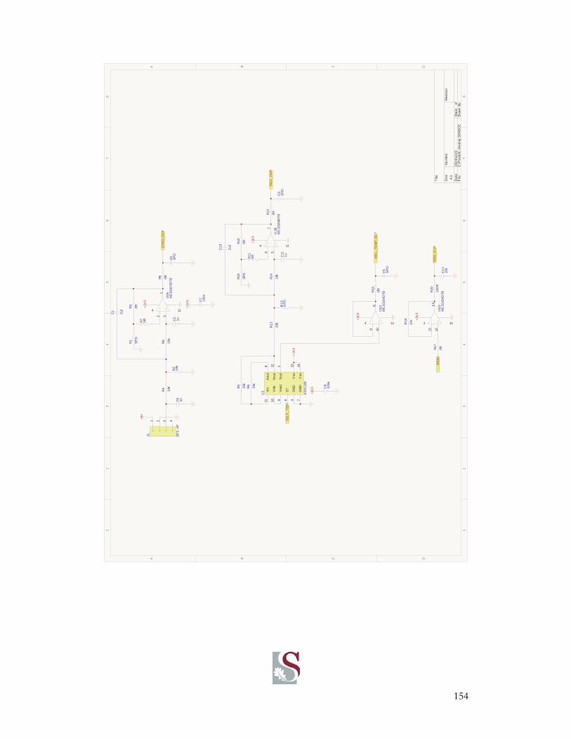
154

11

22

33

44

55

66

77

88

DD

CC

BB

AA

Titl

e

Nu

mbe

rR

evis

ion

Siz

eA

3D

ate:

200

4/11

/20

Shee

t

of

File

:C

:\Pee

te5\

..\An

alog

.SCH

DO

CDr

awn

By:

2 31

114

MC

3320

4DTB

U1A

+5V

1nC6

10k

R4

18k

R2

10k

R8

0RR7

0RR3

SP

O

R1

0RR9

SPO

C3

1uC2

2u2

C1

+3V

3

GYR

O_O

UT

Tout

1

GN

D4

ST

6

GN

D7

Aou

t8

Vm

id9

Vni

n10

Vin

11

Vout

12

Vss

13

Vss

14

AD

XL1

05

U2

+3V

3

100n

C7

+3V

3

100n

C8

+3V

3

9 108

114

MC

3320

4DTB

U1C

+3V

3

SEL

F_TE

ST

33k

R6

33k

R5

0RR15

SP

OC

5

INC

L_TE

MP_

OU

T

13 121

4

114

MC

3320

4DTB

U1D

+3V

3

100

R

R20

10n

C1

2

RSS

I_O

UT

0R

R16

0RR17

RS

SI

1 2 3 4

DF3

, 4P

J1

6 57

114

MC

3320

4DTB

U1B

10k

R13

SPO

R19

10k

R14

0RR11

0RR10

SPO

R18

0RR12

SPO

C4

+3V

3

INC

L_O

UT

1uC11

2u2

C10

155

APPENDIX D : SOURCE CODE

1. Mechanical Position calculation.

The follow block of code demonstrates how the robot’s position could be calculated by

using the change in position of each wheel.

/* __________________________________________________________________________

/ \

| calc_position |

\__________________________________________________________________________/

/ \

| Usage: Calculate the current position based on the wheel movement |

| between now and the last time this function was called. |

| Parameters: None. |

| Returns: None. |

\__________________________________________________________________________/

*/

void calc_position(void)

{

sint32 dl_cntr,dr_cntr;

float dist_l,dist_r;

float theta;

float dist;

ints_dis();

dl_cntr = -(left_step_cntr - prev_l_step_cntr);

dr_cntr = right_step_cntr - prev_r_step_cntr;

prev_l_step_cntr = left_step_cntr;

prev_r_step_cntr = right_step_cntr;

ints_en();

// It is possible for the step_counters to wrap arround 2^32 and 0. If

// this happens, then a very big delta counter will be calculated. Check

// if the delta counter is very big, and if so, correct for the wrapping:

if(dl_cntr > 10000)

dl_cntr = dl_cntr - 2^31;

if(dr_cntr > 10000)

dr_cntr = dr_cntr - 2^31;

// Calculate the distance that each weel traveled:

dist_l = RADIANS_PER_USTEP*WHEEL_D*dl_cntr;

dist_r = RADIANS_PER_USTEP*WHEEL_D*dr_cntr;

pos_theta = pos_theta + ((dist_l - dist_r)/ROBOT_W);

156

if(pos_theta > PI)

pos_theta -= 2*PI;

else if(pos_theta < -PI)

pos_theta += 2*PI;

dist = (dist_l + dist_r)/2.0;

// Update the robot's position:

pos_x = pos_x + dist*cos(pos_theta);

pos_y = pos_y + dist*sin(pos_theta);

} // calc_position

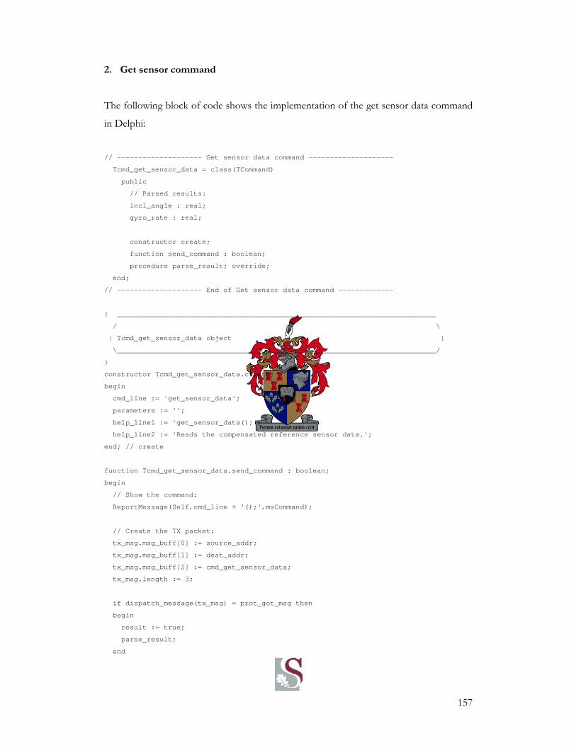
157

2. Get sensor command

The following block of code shows the implementation of the get sensor data command

in Delphi:

// -------------------- Get sensor data command --------------------

Tcmd_get_sensor_data = class(TCommand)

public

// Parsed results:

incl_angle : real;

gyro_rate : real;

constructor create;

function send_command : boolean;

procedure parse_result; override;

end;

// -------------------- End of Get sensor data command -------------

{ ___________________________________________________________________________

/ \

| Tcmd_get_sensor_data object |

\___________________________________________________________________________/

}

constructor Tcmd_get_sensor_data.create;

begin

cmd_line := 'get_sensor_data';

parameters := '';

help_line1 := 'get_sensor_data();';

help_line2 := 'Reads the compensated reference sensor data.';

end; // create

function Tcmd_get_sensor_data.send_command : boolean;

begin

// Show the command:

ReportMessage(Self,cmd_line + '();',msCommand);

// Create the TX packet:

tx_msg.msg_buff[0] := source_addr;

tx_msg.msg_buff[1] := dest_addr;

tx_msg.msg_buff[2] := cmd_get_sensor_data;

tx_msg.length := 3;

if dispatch_message(tx_msg) = prot_got_msg then

begin

result := true;

parse_result;

end

158

else

result := false;

end; // send_command

procedure Tcmd_get_sensor_data.parse_result;

var

tmp : integer;

begin

tmp := ord(rx_msg.msg_buff[3]) shl 8 +

ord(rx_msg.msg_buff[4]);

if(tmp > $7FFF) then

tmp := tmp - $FFFF - 1;

incl_angle := tmp / 10000 * 180/PI;

tmp := ord(rx_msg.msg_buff[5]) shl 8 +

ord(rx_msg.msg_buff[6]);

if(tmp > $7FFF) then

tmp := tmp - $FFFF - 1;

gyro_rate := tmp / 10000 * 180/PI;

// Display the result:

report_string('Incl angle: ' + floattostrf(incl_angle,ffGeneral,4,6) + 'deg.');

report_string('Gyro rate: ' + floattostrf(gyro_rate,ffGeneral,4,6) + 'deg/s.');

end; // parse_result

{ ___________________________________________________________________________

/ \

| End of Tcmd_get_sensor_data object |

\___________________________________________________________________________/

}

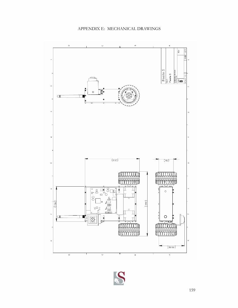
159

APPENDIX E : MECHANICAL DRAWINGS

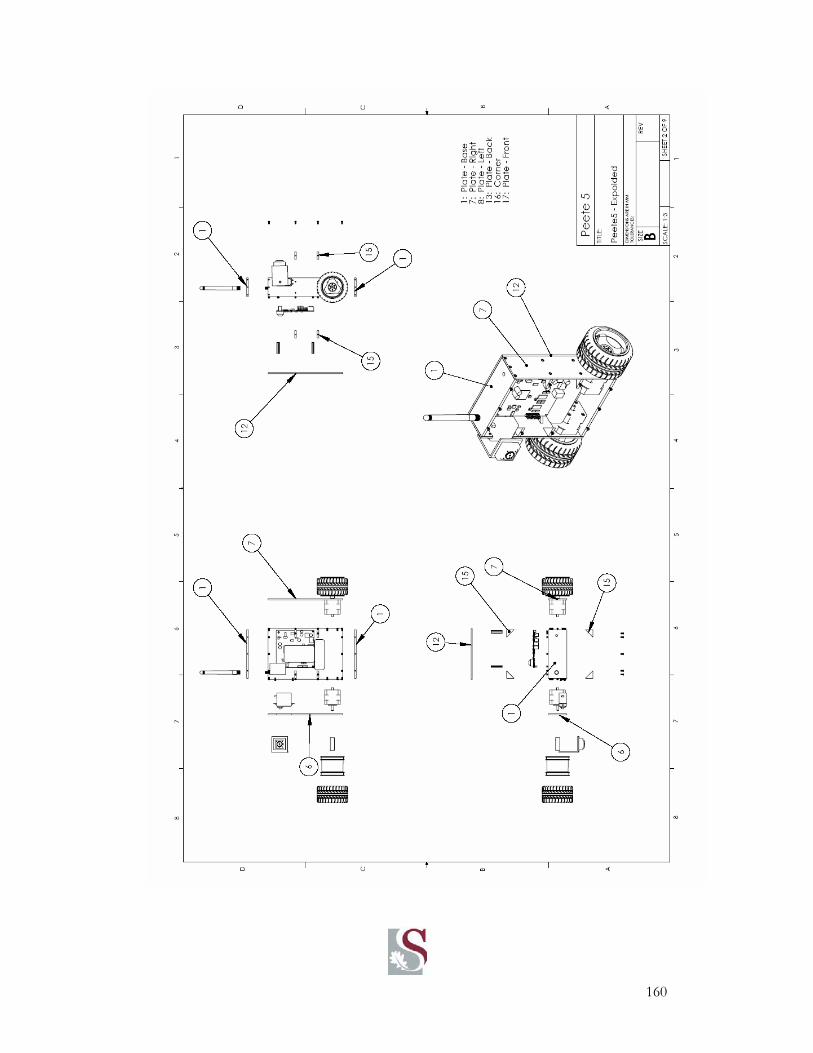
160

161

162

163

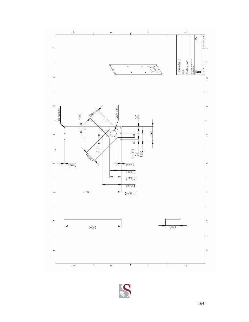
164

165

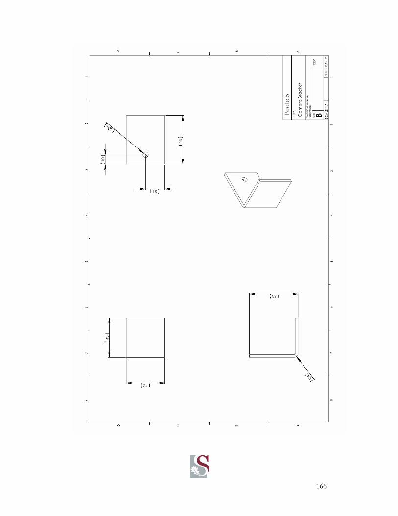
166

167

168

INDEX

A

Absolute

positioning, 1

accelerometer, 85

Active beacons, 1, 2

ADC, 69

Application layer, 18

Artificial landmark

recognition, 1

Artificial Landmark

recognition, 3

autocorrelation, 39,

40

B

Barker, 43

barker code, 4

Barker code, 40

C

CAN, 16, 19, 20, 63,

69, 74, 75

Comms layer, 18

communication

network, 15

compare, 37, 130, 133

correlate, 4, 50, 54

correlates, 39

correlation, 40, 50

CRC, 22

D

data packet, 21

Digital to Analogue

Converter, 10

digitize, 47

F

FSK, 17

G

Global Positioning

System, 2

H

Hardware layer, 19

I

Inertial Navigation,

1, 2

L

least squares estimate,

29

least-squares-

solution, 29

M

matched filter, 50

Matlab, 39

micro stepping, 10

Model Matching, 1,

3

Motherboard, 67

N

NAK, 24

Natural landmark

recognition, 1

Natural Landmark

recognition, 3

Nyquist, 47

O

Odometry, 1

P

position calculation,

15

Protocol layer, 18

pseodo-inverse, 29

PWM), 69

Q

Quantisation noise,

48

R

Radar, 38

Receiver, 42

Relative

positioning, 1

RF, 17, 19, 20, 62,

63, 84, 85

S

schematic library, 7

SCI, 16, 19, 20, 63,

69, 73, 74, 85

side-lobes, 40

SLIP, 20

SPI, 16, 69

stepper motor, 10

T

Transmission

medium, 42

Transmitter, 42

Transmitter Board,

68

U

ultrasonic, 62

ultrasonic range

finding, 15

USB, 16, 19, 20, 76

Date post:	20-Mar-2022
Category:	Documents
Upload:	others
View:	4 times
Download:	0 times

Position control of a mobile robot

Documents