POSITIONIFORCE CONTROL OF MANIPULATORS USED FOR DEBURRING AND GRINDING By DULl HONG Diploma Nanjing Navigation Engineering College Nanjing, China 1982 Submitted to the Faculty of the Graduate College of the Oklahoma State University in partial fulfillment of the requirements for the Degree of MASTER OF SCIENCE May, 1995
Transcript
POSITIONIFORCE CONTROL OF MANIPULATORS
USED FOR DEBURRING AND GRINDING
By
DULl HONG
Diploma
Nanjing Navigation Engineering College
Nanjing, China
1982
Submitted to the Faculty of theGraduate College of the
Oklahoma State Universityin partial fulfillment ofthe requirements for
the Degree ofMASTER OF SCIENCE
May, 1995
POSITIONIFORCE CONTROL OF MANIPULATORS
USED FOR DEBURRING AND GRINDING
Thesis Approved:
Dean of the Graduate College
ii
ACKNOWLEDGMENTS
I wish to express sincere appreciation to Dr. Lawrence L. Hoberock, my major
advisor, for his encouragement, advice, and the many hours ofguidance throughout by
graduate program. Many thanks also go to Dr. Eduardo Misawa and Dr. Ronald D.
Delahoussaye for serving on my graduate committee. Their suggestions and support were
very helpful throughout this study. Financial support during my graduate study was
provided by the Oklahoma Center for Integrated Design and Manufacturing, together with
the Oklahoma Center for the Advancement of Science and Technology.
This work is dedicated to my wife Hui Deng and my parents for their love,
understanding, and encouragement over the years.
iii
Chapter
TABLE OF CONTENTS
Page
I. INTRODUCTION 1
Background 1
Robotic Deburring and Grinding 3
Deburring with Compliant Devices 6
Hybrid PositionIForce Control 8
Impedance Control 11
Hybrid Impedance Contro1. 14
Stability Analysis 15
Objectives of This Study 17
II. DYNAMIC MODELING OF A MANIPULATOR ENGAGED IN
ROBOTIC GRINDING 19
Grinding Mechanics 19
Mechanics ofRobotic Grinding 23
Dynamics ofManipulators 32
SCARA Robot 34
Jacobian Matrix 38
III. CONTROL DESIGN AND ANALySIS 42
Manipulator Performance 42
Control Architecture 46
Impedance Control 49
Hybrid Impedance Contro1. 52
Simultaneous Position and Force Control 57
IV. SIMULATION AND ANALYSIS 62
Simulations 62
Simulations for Impedance Control 68
Results and Analysis for Impedance Control 69
Simulations for Hybrid Impedance Control 77
iv
Results and Analysis for Hybrid Impedance Control 77
Simulations for Simultaneous PositionIForce ControL 81
Results and Analysis for Simultaneous PositionIForce Control 87
V. CONCLUSIONS AND RECOMMENDATIONS 102
Conclusions 102
Recommendations 104
REFERENCES 105
v
LIST OF FIGURES
Figure Page
1. 1 Schematic Diagram of a SCARA Robot Engaged in Grinding 4
1.2 Interaction ofa System and an Environment 16
2.1 Schematic Diagram of Conventional Grinding 20
2.2 Schematic Diagram ofRobotic Grinding Process 24
2.3 The Geometry of Grinding 26
2.4 Schematic Diagram of Two-Arm SCARA Robot 35
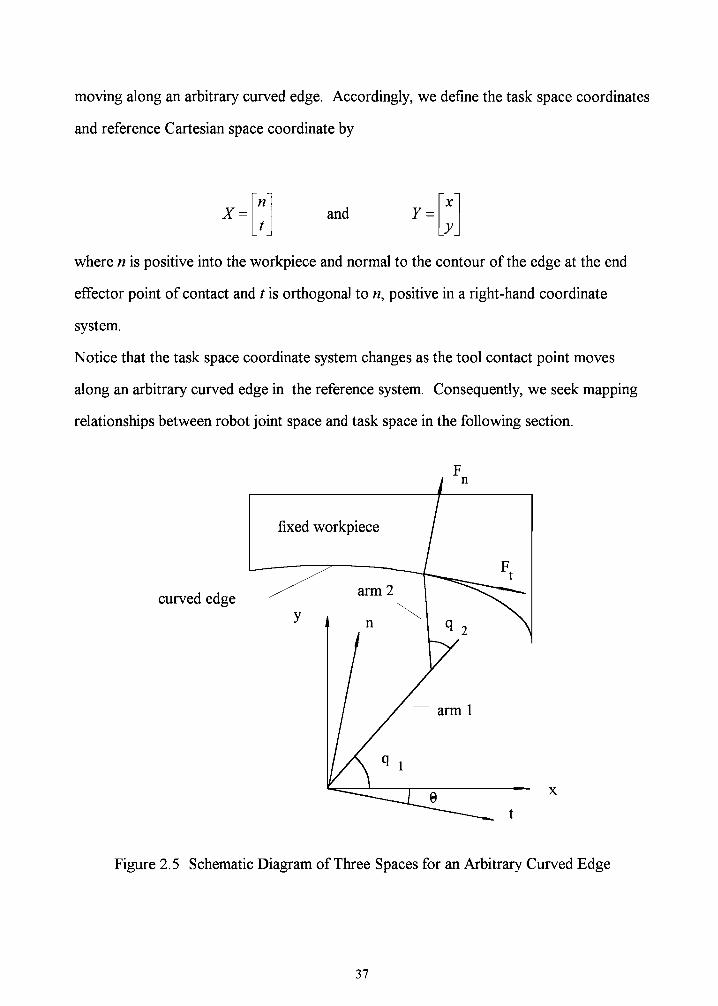
2.5 Schematic Diagram of Three Spaces for an Arbitrary Curved Edge 37
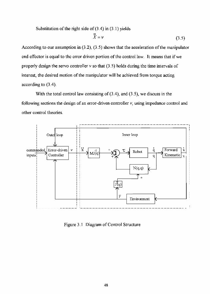
3.1 Diagram of Control Structure 48
3.2 Block Diagram of Impedance Control with Spring-Like Environment 52
3.3 Diagram ofHybrid Impedance Control 56
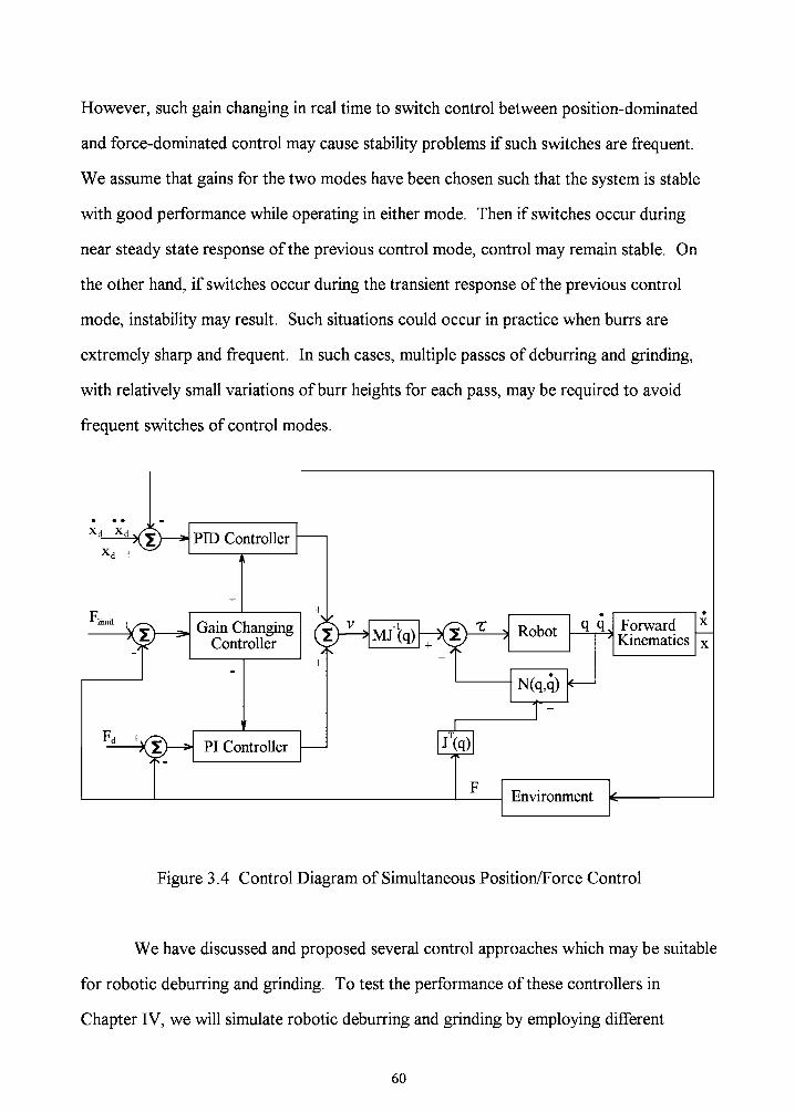
3.4 Control Diagram of Simultaneous PositionIForce Control 60
4.1 Motion History of Two-arm Berkeley SCARA Robot 63
4.2 Schematic Diagram of Geometry ofBurrs 66
4.3 Schematic Diagram ofRobot Configuration in Deburring 67
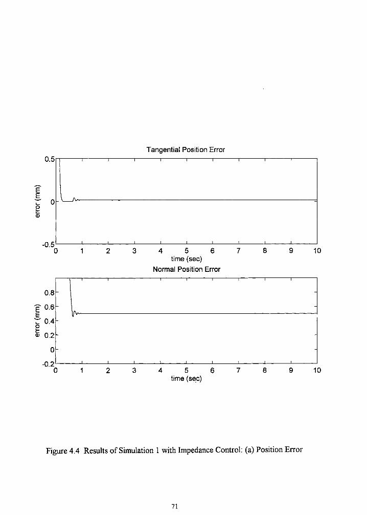
4.4 Results of Simulation 1 with Impedance Control: (a) Position Error 71
4.5 Results of Simulation 1 with Impedance Control: (b) Forces 72
4.6 Results of Simulation 2 with Impedance Control: (a) Position Error 73
4.7 Results of Simulation 2 with Impedance Control: (b) Forces 74
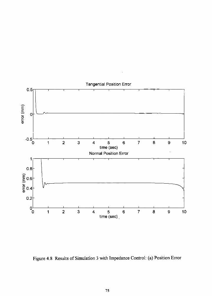
4.8 Results of Simulation 3 with Impedance Control: (a) Position Error 75
4.9 Results of Simulation 3 with Impedance Control: (b) Forces 76
4.10 Results of Simulation 4 with Hybrid Impedance Control: (a) Position Error. 79
4.11 Results of Simulation 4 with Hybrid Impedance Control: (b) Forces 80
4.12 Schematic ofLarge Burrs 85
4.13 Results of Simulation 5 with Simultaneous PositionIForce Control:
(a) Position Error 88
4.14 Results of Simulation 5 with Simultaneous PositionIForce Control:
(b) Forces 89
4.15 Results of Simulation 6 with Simultaneous PositionIForce Control:
(a) Position Error 90
vi
4.16 Results of Simulation 6 with Simultaneous Position/Force Control:
(b) Forces 91
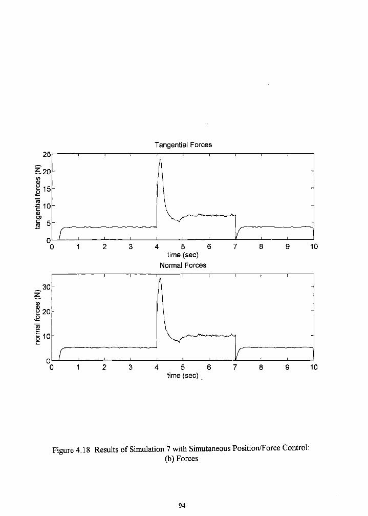
4.17 Results of Simulation 7 with Simultaneous Position/Force Control:
(a) Position Error 93
4.18 Results of Simulation 7 with Simultaneous Position/Force Control:
(b) Forces 94
4.19 Results of Simulation 8 with Simultaneous Position/Force Control:
(a) Position Error 95
4.20 Results of Simulation 8 with Simultaneous Position/Force Control:
(b) Forces 96
4.21 Results of Simulation 9 with Simultaneous Position/Force Control:
(a) Position Error 98
4.22 Results of Simulation 9 with Simultaneous Position/Force Control:
(b) Forces 99
4.23 Results of Simulation 10 with Simultaneous Position/Force Control:
(a) Position Error 100
4.24 Results of Simulation 10 with Simultaneous Position/Force Control:
(b) Forces 101
vii
B
Fact
Ke
Ki,Ki,Kd
Kf/
/1' /2M
M d
M t
q
s
NOMENCLATURE
Target damped matrix
Environmental damped matrix
Width of cut
Centrifugal and Coriolis term matrix in joint space
Centrifugal and Coriolis term matrix in Cartesian or task space
Diameter of grinding wheel
Depth of cut
Interaction force vector
Actuator force vector
Normal and tangential (cutting) grinding force
Static friction vector in joint space
Static friction vector in Cartesian or task space
Gravity term vector in joint space
Gravity term vector in Cartesian or task space
Jacobian matrix
Jacobian matrix mapping from joint space to Cartesian space
Jacobian matrix mapping from Cartesian space to task space
Target stiffness matrix
Environmental stiffness matrix
Proportional, integral, derivative gain matrices
Force gain vector
Chip length
Length of link 1 and link 2
Inertial matrix in joint space
Target inertial matrix
Inertial matrix in Cartesian/task space
Joint coordinate vector.
Laplace operator
viii
xz
Specific energy for grinding process
Speed ofworkpiece
Peripheral wheel speed
Velocity along normal and tangential direction
Position vector in ask space
Impedance matrix
Environmental impedance vector
Volume removal rate
Torque vector, control input
Coefficient of grinding friction
Grinding Coefficient in normal and tangential direction
Metal removal parameter
ix
CHAPTER I
INTRODUCTION
Background
A burr is an undesired projection of material formed as the result of cutting,
shearing or casting processes. It is unavoidable in many machining operations. Since
burrs can cause interference in the fit of components in assembly, defects in finished
components, and injuries to workers, they must be removed. Very often, deburring is not
sufficient for some parts, and more precise finishing, called edge finishing must be done to
achieve desired contours. At present, deburring and edge finishing are costly and labor
intensive. It is common to deburr or grind edges or surfaces manually in off-line
processes, resulting in extra material handling, increased processing time, and lower
quality products. In some highly automated machining processes, deburring or edge
grinding operations may require a significant portion of the time and cost, compared with
other machining operations. It is desirable to develop automatic deburring and edge
grinding to reduce manual work as much as possible, integrating deburring or edge
grinding operations with automated on-line process to streamline machining operations.
Because of its success in other manufacturing operations, the use of robotics appears to
offer potential for automatic deburring and edge grinding.
Automation in manufacturing industries has made extensive use of industrial robots
[1], particularly in those cases where operations are repetitious and require moderate
1
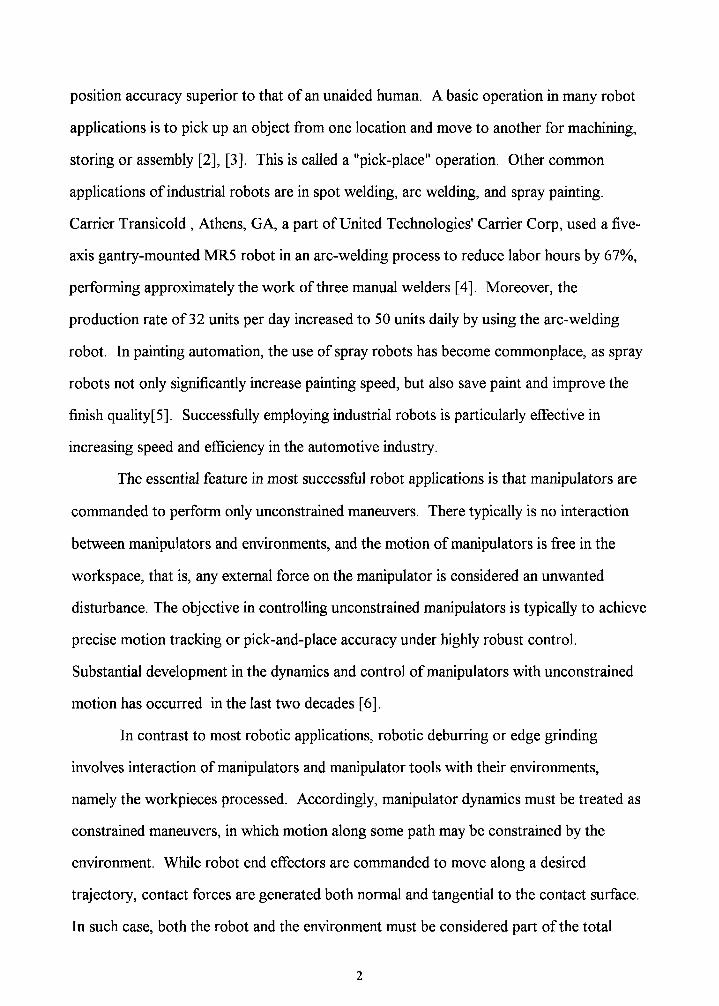
position accuracy superior to that of an unaided human. A basic operation in many robot
applications is to pick up an object from one location and move to another for machining,
storing or assembly [2], [3]. This is called a "pick-place" operation. Other common
applications of industrial robots are in spot welding, arc welding, and spray painting.
Carrier Transicold , Athens, GA, a part ofUnited Technologies' Carrier Corp, used a five
axis gantry-mounted MR5 robot in an arc-welding process to reduce labor hours by 67%,
performing approximately the work of three manual welders [4]. Moreover, the
production rate of32 units per day increased to 50 units daily by using the arc-welding
robot. In painting automation, the use of spray robots has become commonplace, as spray
robots not only significantly increase painting speed, but also save paint and improve the
finish quality[5]. Successfully employing industrial robots is particularly effective in
increasing speed and efficiency in the automotive industry.
The essential feature in most successful robot applications is that manipulators are
commanded to perform only unconstrained maneuvers. There typically is no interaction
between manipulators and environments, and the motion of manipulators is free in the
workspace, that is, any external force on the manipulator is considered an unwanted
disturbance. The objective in controlling unconstrained manipulators is typically to achieve
precise motion tracking or pick-and-place accuracy under highly robust control.
Substantial development in the dynamics and control of manipulators with unconstrained
motion has occurred in the last two decades [6].
In contrast to most robotic applications, robotic deburring or edge grinding
involves interaction of manipulators and manipulator tools with their environments,
namely the workpieces processed. Accordingly, manipulator dynamics must be treated as
constrained maneuvers, in which motion along some path may be constrained by the
environment. While robot end effectors are commanded to move along a desired
trajectory, contact forces are generated both normal and tangential to the contact surface.
In such case, both the robot and the environment must be considered part of the total
2
dynamic system. Manipulators in constrained maneuvers require control ofboth motion
and force, or regulation between motion and force. Control of interaction force and
motion simultaneously is fundamental to robotic deburring and grinding. Because control
of a constrained manipulator requires high precision, force and position feedback, and
advanced control strategies, it is often difficult to implement. Developing an effective and
efficient scheme for force control of robots associated with deburring and edge grinding is
therefore an attractive research problem.
Robot Deburring And Edge Grinding
Robot deburring and edge grinding consists of a robot carrying a finishing tool
traveling along a desired path while the finishing tool, driven by an independent actuator,
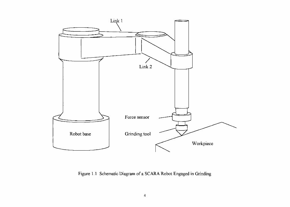
rotates at high speed for metal removal. Figure 1 shows a simple example of a deburring
or edge finishing process using a SCARA (selective compliance articulated robotic arm)
robot with a grinding wheel mounted on the end effector of the robot. While the robot is
commanded to follow a desired trajectory, it traverses the grinding wheel along the edge
of a workpiece. Material removal occurs as the grinding wheel or finishing tool cuts into
the workpieces. While traditional grinding machines may be limited to motion of the tool
along simple geometric curves, such as straight lines or circles, a finishing tool mounted
on a robot can easily travel along complex spatial curves. This allows more flexibility for
robot deburring or grinding in complex tasks.
The aim of robot deburring and edge finishing is to produce, by metal removal,
finished surfaces along commanded trajectories within allowed dimensional tolerances and
surface roughness. The cutting performance of deburring and grinding tools is primarily
dependent on three process parameters [7]: rotation speed of the cutting tools, depth of
cut, and relative traverse speed of grinding tool and workpiece. For a given geometric
configuration and type of tool, the rotation speed of the finishing tool primarily influences
3
Link 1
\
Robot base
Force sensor
Grinding tool
Workpiece
Figure 1. 1 Schematic Diagram of a SCARA Robot Engaged in Grinding
4
the finish of edges or surfaces. Within the stable grinding stage, increasing the rotation
speed of grinding tools usually improves the finish, provided other grinding conditions
remain contact. On the other hand, the depth of cut and relative traverse speed of the
grinding tool govern the material feed rate of the grinding process, and therefore
determine the grinding force generated [7].
Similar to other automated processes, robot deburring and grinding will perform
best when the disturbance or input is constant, such as a "continuous" bur with constant
width, height, and shape. This would imply an uniform material feed rate and depth of
cut. On the other hand, a robotic deburring or grinding process should be robust to
maintain acceptable performance under fluctuations of inputs and disturbances within
allowable ranges. In many cases, workpieces are fixed, such that material feed rates must
be controlled by adjusting the robot's position and traversing speed along desired edges or
surfaces.
Force control is central to robot deburring and edge grinding, and the forces
generated by the cutting process can be resolved into components normal and tangential to
the trajectory at an idealized "point" of contact between the tool and workpiece.
Maintaining the normal force within desirable limits usually will also maintain the
tangential force within limits, both ofwhich are essential for satisfactory cutting
performance. Zero normal force implies loss of contact, with no cutting action; excessive
normal or tangential force may cause stall of the grinding tool, or damage to the tool,
workpiece, or robot. In fact, for many applications, when the interacting force exceeds
specific limits, chattering may occur before tools or the robot system are damaged.
Chattering is an undesired high frequency oscillation between contact and loss-of-contact
between tool and workpiece. It degrades the quality of the edge or surface finish and
ultimately will damage the tool. It can be avoided with appropriate force control.
There are two principal strategies for force control currently employed in robot
deburring or edge grinding processes. One is to utilize a compliant device connecting the
5
robot end-effector to the cutting tool to compensate for interacting forces and position
uncertainty of environments [8],[9]. Use of such compliant devices allows commercial
robots to be used directly without modification ofbuilt-in controllers. The second
strategy is to directly mount the finishing tool on the end effector of the robot and employ
force control by means of an advanced robot controller that integrates end effector motion
control with a force feedback loop.
In the first strategy, the compliant device absorbs much of the contact force
variation, such that the required robot motion compensation control is less demanding.
Depending upon requirements, this may allow commercial robots to be directly employed
without much modification. Some innovative designs of compliant devices, such as the
RCC(Remote Center Compliance)[IO], have been applied to deburring. However, any
type of passive or active compliant devices may increase the end effector inertia of the
robot system, adversely affecting performance. Allowable inertia should be carefully
designed, considering the grinding tool, part contour, feed rate, and desired accuracy.
Typically, large inertia of compliant devices limit the applications of such devices.
Without compliant devices, the second approach usually requires more accurate and
robust control algorithms than are available on commercial robots. Although this strategy
is complex and difficult to implement, it is flexible and versatile. As robot controllers and
sensors improve, this method will become more feasible.
Deburring with Compliant Devices
Early research in robotic deburring employed compliant elements at the end
effector. Kramer et al. [8] first explored the fundamental mechanisms of robot deburring.
Based on the stiffness of an end effector required for a specific deburring task, Kramer, et
al. designed a passive single-degree-of-freedom end effector(PSDF) to hold a finishing
rotary file. This device provided initial compliance for force variation and position
6
uncertainty occurring during the deburring process. With the PSDF end effector mounted,
a robot with open loop position control was able to achieve stable deburring results.
However, deburring without force feedback, such as initially used by Kramer, et al., may
result in surface finishes that are insufficiently smooth. Thus, a new strategy was
proposed to integrate a force feedback signal. This approach employed a robot position
control loop and a fine motion control loop. The fine motion control loop was robot
independent and utilized a micromanipulator to adjust the relative position of a workpiece
relative to the end effector based on a feedback signal from a force sensor. For the robot
position control loop, the robot performed the programmed function with no
communication from the end effector force signal. This allows a robot to be directly
applied to the process without knowledge of the robot's dynamics and controller
architecture. An active x-y positioning table mounting with a force sensor was developed
in the experiment to implement the performance of the mirocmanipulator in the fine
motion loop.
Kazerooni, et al. [9] investigated this strategy in the frequency domain and pointed
out that for a deburring robot, stiffness in the normal and tangential directions should be
designed to be low and high, respectively, so that the system is robust relative to robot
oscillations, robot inaccuracy, and fixturing errors. On the other hand, the deburring
process requires a large robot stiffness in the normal direction and small stiffness in
tangential direction to achieve good deburring performance. This requirement causes the
end effector to ignore the interaction force in the normal direction and stay close to the
desired trajectory. These conflicting design requirements raise the control problem for this
strategy together with difficulty in practical implementation. A compliant device for the
end effector and an active x-y positioning table were designed and implemented to
overcome these difficulties.
Recently, Koelsch [11] reported that General Dynamics used flexible-abrasive
brushes with a "constant force" device mounted on the end effector of an industrial robot
7
to debur and chamfer bulkheads and other complex parts for the F-16 fighter. The
combination of the innovative tooling and robot control allowed robot deburring to
successfully achieve the desired results. From a control viewpoint, the wire brushes
function as a highly compliant device to compensate for position uncertainty and fixturing
errors.
Hybrid PositionIForce Control
Traditional approaches dealing with free motion control of manipulators without
contact with the environment focus mainly on the inertial effects on performance. In
contrast, force control for manipulators constrained by environments must deal with the
combined influence of robot inertia and compliances of robot and workpiece.
Effective force control of manipulators requires integration of task modeling,
trajectory generation, force and position feedback, control, and stability. It requires good
understanding of task goals and good modeling, such that an effective control strategy and
trajectories may be planned. It also requires control such that stable and precise
performance of the manipulator is achieved. Since measurement of force and position may
be noisy, effective filtering techniques may be needed. An effective force and position
control algorithm should fulfill all these requirements.
Much research has been done on the force control of manipulators involved in
constrained motion, and an overview of available force control algorithms is given in [12].
Whitney classified force control approaches, based on the relation of the control input and
output, into several types of methodologies, including: stiffness control, damping control,
impedance control, hybrid force/position control, and explicit/implicit force control.
The fundamental differences in various force control methods associated with
manipulators may be classified into two types of control architectures: hybrid
force/position control [13],[14],[15] and impedance control [16] - [24]. In hybrid
8
force/position control, force is commanded and controlled along those directions
constrained by the environments, while position is commanded and controlled along those
directions in which manipulators is unconstrained and free to move. Usually, the force and
position control directions are orthogonal, and a particular control law may be applied in
the individual direction for the regulation of force errors or position errors. On the other
hand, impedance control focuses on the relationship between the interaction force and the
end-effector position. Instead of controlling force or position individually, impedance
control attempts to regulate the interaction force by controlling the amount of compliance
or impedance in the manipulator. Using impedance control, a designer can specify a target
impedance, the desired relationship between the interaction force and end-effector
position, and control the position to maintain the desired interaction force. We first
review hybrid position/force control strategies.
Hybrid position/force control is used for control tasks requiring force control in
some directions and motion control in other directions. It requires the task description to
be decoupled into elemental subtasks, which are defined by a particular set of constraints.
Typically, a position constraint exists in the direction normal to the contact surface, and a
position control subtask is formulated with a force constraint along the tangential direction
of the contact surface. Thus, control is partitioned into a set of orthogonal constraint
directions. With each subtask, pure force control or pure position control algorithms may
be applied. For instance, in the force control direction, force is commanded and
controlled explicitly. The key to hybrid control is the specification of a task constraint
frame, either a natural constraint frame or an artificial constraint frame. Mason [13]
discussed kinematic constraints imposed on manipulator motion due to a particular task
geometry. The discussion in this paper is quite general and includes many types of
constraints that can occur during a variety of tasks.
Raibert and Craig [14] first developed hybrid force/position control, with the
position and force loops operating under different control laws (PID for position and PI
9
for force) to control a manipulator. Position was measured with joint-mounted sensors
and a force signal was obtained by a wrist-mounted force sensor. A selection matrix was
introduced to indicate the particular constraint in each degree-of-freedom, and this was
used to apply compensation functions to determine the actuator drive signal for each joint.
Experiments were conducted using a two-axis Scheinman robot to test the designed
controller. Different levels of forces were commanded in the normal direction while
motion was controlled simultaneously in the tangential direction. While the results
showed stable control, force error developed, together with overshoot and unspecified
position errors in the normal direction.
Yoshikawa et al. [15] extended Raibert and Craig's hybrid control approach to a
more general case where the full dynamics of the manipulator were considered, and the
end effector constraint was explicitly described by constraint hypersurfaces. To design a
hybrid controller, nonlinear state feedback was introduced to linearize the manipulator
dynamics. Then servo-controllers were designed for both position and force control based
on the linearized model. A two degree-of-freedom assumption was employed to design
the servo controllers, which took account ofboth command response and robustness for
the modeling errors and disturbances.
The disadvantage of hybrid force/position control algorithms is the neglect of
manipulator impedance, and thus inability to regulate the relation of force to position. In
the position control direction, forces are either neglected or considered as disturbance,
while in the force control direction motion errors are left uncontrolled. On the other hand,
hybrid force/position control requires explicit and accurate descriptions of environmental
dynamics in term of position and force constrains. For some complex tasks, this will
present difficulties in formulation and computation.
10
Impedance Control
The impedance of a dynamic system is defined from a linear relationship between
displacement and force given by:
F=ZM (1.1)
(1.2)
where M is an m x 1displacement vector of the system from its equilibrium position, F is
an n x 1 vector of external forces applied to the system, and Z is an n x m impedance
matrix. For the static case, Z is simply the stiffness K, a real-valued nonsingular stiffness
matrix with constant elements. The stiffness matrix primarily characterizes the behavior of
a system in constrained maneuvers. Large entries in the stiffness matrix imply large
interaction forces, while small entries in the matrix allow for a considerable amount of
motion of the system in response to interaction forces.
The dynamic impedance characterizing the behavior of an n-dimensional linear
dynamic system contains inertial, damping, and stiffness elements. It may be defined using
Laplace transform natation as:
Z = M d s2 +Bs+K
where s is the Laplace variable and Md, B, and K are n x n positive matrices representing
inertial, damping, and stiffness elements of the system, respectively.
Impedance control regulates the impedance of a system, instead of controlling the
motion of the manipulator or the interaction force individually, as in hybrid force/position
control. By controlling the manipulator motion and specifying the impedance, a designer
can ensure that the manipulator will be able to maneuver in a constrained space while
maintaining appropriate contact force. Impedance control is considered a combination of
pure position control and pure force control. It approaches pure position control when
stiffness approaches infinity. In contrast, if the stiffness approaches zero, it approaches
pure force control.
11
The initial idea of impedance control derives from Salisbury's stiffness control [16],
which used a static form of impedance. The desired relationship of contact force and
manipulator motion was modeled as the stiffness of a spring. Active force control was
applied to make the manipulator behave as the desired spring. By specifying the desired
spring stiffness, designers were able to achieve the desired interaction force. Essentially,
Salisbury's stiffness control is a PD (proportional plus derivative) type control law with
force feedback, which is mapped to modify manipulator position.
Whitney [1 7] developed another approach, called damped force control, as another
form of impedance control. In damped force control, the desired relationship of the
interaction force to manipulator motion was modeled as a dashpot. The difference
between damped control and stiffness control is that the former uses manipulator position
as commanded input, while the later uses manipulator velocity as the commanded input.
Hogan's impedance control [18], [19] generalized the work of Salisbury and
Whitney by forcing the dynamic behavior of any manipulator to approximate a generic
linear second-order system with inertia, damping, and stiffness. The concept of impedance
control is to reshape the dynamics of the manipulator such that the closed loop system
behaves as a mass-dashpot-spring system, whose parameters (inertial, damping, and
stiffness matrix) can be specified by the designer based on the desired behavior of the total
system. Hogan's paper series [18] explained the fundamental theory of impedance control.
Using causality and bond graph theories, he presented a thorough study of the mechanics
of interaction between physical systems. He demonstrated the necessity of controlling the
impedance of manipulators so that the desired dynamic interaction between a manipulator
and its environment could be achieved. Hogan also investigated control both with force
feedback and without force feedback. Finally, a simple control law for impedance control
was developed for a manipulator with a desired Cartesian impedance. In his later work
[19], Hogan conducted experiments with a robot to follow a simple edge to verify the
12
validity of impedance control. The results showed that proper design of an impedance
controller can guarantee the stability of manipulators in contact with environments.
A sophisticated design method for impedance control was developed by Kazerooni
et al. [21], in which both target dynamics and stability robustness in the presence of
bounded model uncertainties are considered. Full state feedback and feedforward force
was investigated to achieve the target dynamics and global stability. The control
approach, however, was established based on a linearized model of a manipulator in a
small neighborhood around the equilibrium position, with an assumption of small
perturbations in position; the nonlinear velocity term in the manipulator dynamics was
ignored. A controller for a plane position table was designed by this method, and
experiments were conducted to study the interaction between the table and a stiff wall.
Recently, experiments [27] were carried out on a direct drive robot manipulator to
investigate the impedance control method with both a linear (Kazerooni, 1986) and a
nonlinaer controller (Colgate and Hogan, 1988). The results from both controller were
compared, showing that the behavior of the manipulator with a linear controller was
inferior when the manipulator engaged in constrained maneuvers. However, the
experiments investigated only cases in which the input was a constant, that is, set-point
control. Controlled behavior with a dynamic input is needed for more general cases, such
as deburring and grinding.
Impedance control has attracted much study, both theoretically and experimentally.
It is considered a general control method for manipulators with constrained and
unconstrained motion. However, the design and implementation of impedance control is
not as intuitive as hybrid position/force control. It is also difficult to map the desired
dynamic behavior and performance of the controlled system into the target impedance
relationship. In addition, almost all of the literature dealing with impedance control is
limited to linear environments. Nonlinear environments raise significant complexities in
designing and implementing impedance control. Furthermore, it is difficult to design a
13
impedance controller to achieve desired performance and preserve stability with
robustness for bounded uncertainties.
Hybrid Impedance Control
Hybrid impedance control is a combination of hybrid position/force control and
impedance control. It breaks down a task into two subtasks in orthogonal directions,
along which either impedance force control or impedance position control is applied.
Noticing the advantages both hybrid control and impedance control, Anderson and Spong
[24] first proposed the concept of hybrid impedance control. They modeled manipulators,
environments and their interaction as an electrical network and used the Norton and
Thevenin equivalents in the network to establish a duality principle, leading to a rule to
construct target impedances of manipulators and select appropriate control schemes. The
dynamics of an environment were modeled as a linear impedance, and the manipulator
interacting with the environment was be controlled as the dual of the environmental
impedance. According to their proposals, impedance relationships could be classified into
three types of impedance: inertial, resistive, and capacitive, given byo Inertial impedance
IZv(O)I= c Resistive impedance
00 Capacitive impedance
(1.3)
where 0< c < 00. In Laplace notation, these types of impedances take following forms
respectively [24]:
Mds
Zv(s) = B
Mds+B+K / s
Inertial impedance
Resistive impedance
Capacitive impedance (1.4)
If the environmental and manipulator impedances are modeled or chosen to be one
of the above impedance relations, then the duality principle can be applied. That is, if the
14
environmental impedances are capacitive, then there will be force control with
noncapacitive manipulator impedances; if the environmental impedances are inertial, then
position control with noninertial manipulator impedances will be applied; if the
environmental impedances are resistive, either force control with inertial manipulator
impedances or position control with capacitive manipulator impedances is applied.
Hybrid impedance control is more similar to hybrid position/force control than to
impedance control. Force and position can be commanded explicitly once the impedance
of the environment is defined or modeled. The duality principle is useful for designers to
choose the control approach and target impedance for a desired task requirement. We will
investigate hybrid impedance control further in our deburring study in Chapter III.
Stability Analysis
Stability analysis is a difficult issue in designing a controller for manipulators with
constrained motion. This is because guaranteeing stability of manipulators in
unconstrained maneuvers does not guarantee stability of manipulators after they interact
with environments. Few discussions in the literature address stability analysis for hybrid
position/force control primarily because the design strategies are so intuitive. In
Yoshikawa's work [15], stability of manipulators was ensured by considering the robust
design of a two degree-of-freedom control law.
For impedance control, as Kazerooni pointed out [22], the stability must address
two important issues: stability of target dynamics and the global stability of the dynamic
system and its environment. Stability of target dynamics is ensured by the proper choice
of target impedance parameters, Md, B, and K. If these target impedance matrices are
real, symmetric, and positive definite, the target dynamics are stable.
Stable target dynamics are necessary for the global stability of the complete
dynamic system; however, this dose not guarantee stability of the total system after
15
contact. It is much more difficult to guarantee global stability of the complete dynamic
system, including nonlinear dynamics of manipulator and environment.
For linear, stable environments, Kazerooni et al. [21] gave a sufficient condition
with informal proof: showing the stability of the complete system can be achieved
provided linear, stable target dynamics are designed with symmetric, positive definite
inertial, damping, and stiffness matrices. However, An and Hollerbach [25] showed that a
forth-order linear system, consisting of a manipulator with a force sensor and
environment, employing impedance control for contact tasks with a very stiff environment
became unstable.
Colgate and Hogan [26] presented a necessary and sufficient condition to
guarantee the stability of a linear model of manipulators coupled at a single interaction
port to a linear, passive environment. Using the Nyquist criterion for a system depicted in
Figure 1.2, they concluded that the controlled system A(s) being positive real is a
necessary and sufficient condition to ensure stability when coupled to any passive,
Hamiltonian environment B(s). A simulation with a proposed linear model for a
manipulator together with actuator and transmission dynamics was usd to verify the
proposed design method and stability condition.
f(s)A(s)
B(s)v(s)
A(s) -- controlled system
B(s) -- the environment
Figure 1.2 Interaction of a System and an Environment
However, McCormick and Schwartz [27] used such a controller in a direct drive robot
and discovered experimentally that the manipulator coupled with an environment became
16
unstable when the force feedback was high no matter how hard (steel) or soft (rubber) the
environment. This may have been caused by modeling the interaction as directly coupled
linear systems in the derivation of stability conditions.
For the general case, stability mechanisms in impedance control are poorly
understood, such stability is dependent upon manipulator dynamics, the nature of the
contact environment, and target impedance parameters.
Objectives of This Study
Previous work reproted in the literature on robotic deburring and edge grinding
has utilized a separate force control loop to monitor the interaction between manipulators
and environments. Force errors obtained from this control loop were mapped into motion
modifications, which were added to the command input of the robot position control loop.
Speed of response was limited by several issues associated with this strategy, such as
mechanical resonance, communication time delay, and programming compatibility. In
contrast, integrated robotic position/force control offers the advantages of a more efficient
force control computation and coordinated force and motion control. With the advent of
faster computers and high performance servos, it has become more attractive to integrate
force control into overall robot position control.
This research investigates position/force control of the dynamics of simple SCARA
manipulators operating in constrained environments, focusing on the application of
manipulators in deburring and edge grinding processes. We employ modeling and
simulation to investigate different control algorithms and their achievable results for a
sample robot engaged in deburring and edge grinding. Through this study, we propose
theoretical control strategies that could later be tested experimentally. In the following
chapters, we describe a new approach to the control of robotic deburring and edge
grinding to provide more accurate, flexible, and robust control than heretofore possible.
17
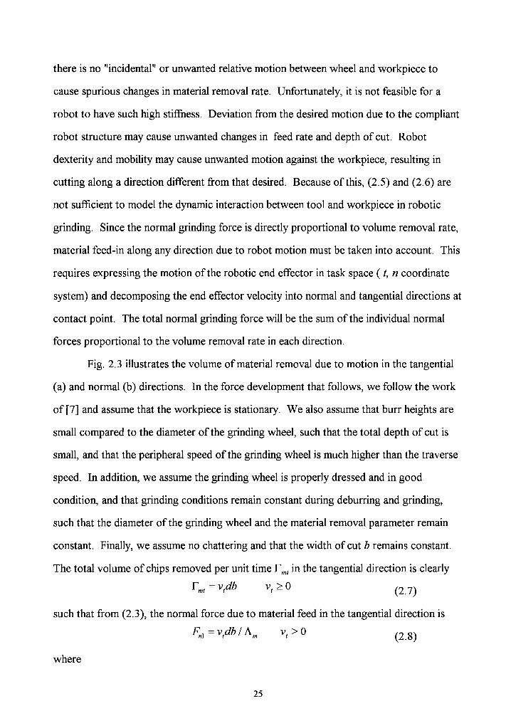
Next chapter first reviews the mechanics of grinding processes in order to develop
a more practical force model for robotic deburring and grinding. We use empirical and
experimental results from conventional grinding process research, together with some
simplifying assumptions to derive interaction force models for robot control purposes.
In chapter 2, we present dynamic models for grinding and manipulator motion in
the presence of contract and grinding forces.
Chapter 3 presents a new force and motion control algorithm for robotic deburring
and grinding. Impedance control and hybrid impedance control are also investigated in
this chapter.
In Chapter 4, edge following and deburring/grinding processes are simulated for
selected workpiece edge contours so as to test and compare between the control
algorithms discussed in this study. Analysis and discussion of the simulation results are
also presented.
We present conclusions of this study and recommendations for future work in
Chapter 5.
18
CHAPTER II
DYNAMIC MODELING OF A MANIPULATOR ENGAGED IN
ROBOTIC GRINDING
Appropriate modeling of dynamic systems is usually essential for designing and
analyzing controllers for these systems. Robotic deburring and grinding incorporates the
dynamic behavior of conventional grinding, with complexities added due to the somewhat
compliant nature of robotic arms. In this chapter, we develop a model for the interaction
forces in robotic deburring and grinding. The control strategy discussed in the remaining
part of this thesis is based on the model obtained here. Manipulator dynamics are also
developed in this chapter.
Grinding Mechanics
Conventional grinding process is a complicated and poorly understood machining
process. Usually, a grinding wheel is considered a complex tool with thousands ofvery
small metal cutting "teeth" sprinkled along the periphery of the wheel [7]. The abrasive
grains are all different, with irregular shapes, and are randomly oriented on the grinding
wheel. Most grains have large negative rake angles causing them to slide rather than cut.
Thus, the interaction process between grains and workpiece consists of cutting, plowing,
and rubbing[28]. The stochastic nature of the grains makes it very difficult to analyze the
grinding process and even more difficult to model the dynamics of grinding. Thus, there is
19
no good analytically-developed mathematical model for the conventional grinding process.
An attempt to suitably model the process will, however, provide us with a better overall
understanding and help to interpret the forces produced by this process.
J. Robotics and Automation, vol.4, no.6, pp. 677-686, December 1988.
21. Kazerooni, H., Sheridan, T., and Houpt, P., "Robust Compliant Motion for
Manipulators, Part I: The Fundamental Concepts of Compliant Motion, Part II:
106
Design Method," IEEE J. Robot. Automation, vol. RA-2, no.2, pp.83-91, June
1986.
22. Kazerooni, H., "On the Robot Compliant Motion Control," ASME J. Dynam.
Sys. Meas. Control, vol.lll, pp.416-425, September 1989.
23. Kazerooni, H., Kim, S., and Waibel, B. J., "Theory and Experiment on the
Stability ofRobot Compliance Control," ASME Winter Annual Meeting at
Chicago, DSC-vol. 11, pp. 87-101, November 1988.
24. Anderson, R., and Spong, M., "Hybrid Impedance Control ofRobotic
Manipulators," IEEE J. Robot. Automat., vol. 4, no.5, pp. 549-556, Oct. 1988.
25. An, C. H., and Hollerbach, J. M., "Dynamic Stability Issures in Force Control of
Manipulators," Proceedings of the American Control Conference, pp. 821-825,
1987.
26. Colgate, E., and Hogan, N., "Robust Control ofDynamically Interacting
Systems," Int. J. Control, vo1.48, no. 1, pp.65-88, 1988.
27. McCormick, W., and Schwartz, H. M., "An Investigation of Impedance Control
for Robot Manipulators," The International Journal ofRobotics Research, vol. 12,
no.5, pp.473-489, 1993.
28. King, R. I., and Hahn, R. S., "Handbook ofModern Grinding Technology,"
Chapman and Hall, New York, 1986.
29. Hahn, R. S., and Lindsay, R. P., "Principles of Grinding," 5 part series in
Machinery, July-Nov. 1971.
30. Craig, John J., Introduction to Robotics Mechanics & Control, Addison-Wesley
Publishing Company, Inc., 1986.
31. Kang, C. G., Kao, W. W., Boals, M., and Horowitz, R., "Modeling Identification
and Simulation of a Two Link Scara Manipulator," The Winter Annual Meeting of
ASME, Chicago. 1988, vII, 393-407.
107
32. Craig, J. J., Hsu, P, and Sastry, S. S., "Adaptive Control ofMechanical
Manipulators," The International Journal ofRobotics Research, vol.6, no.2,
pp.16-28, 1987.
33. Slotine, J.-J. E., and Li, W, "On the Adaptive Control of Robot Manipulators,"
The International Journal ofRobotics Research, vo1.6, no.3, pp.49-59, 1987.
34. Lucca, D, Private Conversation. Feb., 1995.
35. Grat: T. L., "Deburring, Finishing and Grinding with Robots," SME Machining
Technology, vol. 5, no. 3, pp. 1-7, 1994.
36. MATLAB Reference Guide. (1992). Natick, Mass.: The Math Works, Inc.
108
VITA
Duli Hong
Candidate for the Degree of
Master of Science
Thesis: POSITIONIFORCE CONTROL OF MANIPULATORS USED FORDEBURRING AND GRINDING
Major Field: Mechanical Engineering
Biographical:
Personal Data: Born in Jiazhi, Guangdong, China, August 6, 1963, the son ofXiangyou Hong and Yuqiong Fang.
Education: Graduated from Jiazhi High School, Guangdong, China, in July1979; received a diploma in Mechanical Engineering from NanjinNavigation Engineering College, Nanjin, China, in July 1982; receivedMaster of Science Degree in Mechanical Engineering in ChongqingUniversity, Chongqing, China, in April 1988; completed requirements forthe Master of Science Degree at Oklahoma State University in May 1995.
Professional Experience: Mechanical Engineer, Guangzhou Mechanical &Electrical Engineering company, Guangzhou, China, from August, 1982,to August, 1985; Project Engineer, Guangzhou M&E EquipmentTendering Corp., Guangzhou, China, from May, 1988, to December,1992; Graduate Research Assistant, Department ofMechanicalEngineering, Oklahoma State University, from September, 1993, to May,1995.