87 Positive feedback trading under stress: evidence from the US Treasury securities market Benjamin H Cohen and Hyun Song Shin, 1 Bank for International Settlements, London School of Economics Abstract A vector autoregression is estimated on tick-by-tick data for quote changes and signed trades of two-year, five-year and 10-year on-the-run US Treasury notes. Confirming the results found by Hasbrouck (1991) and others for the stock market, signed order flow tends to exert a strong effect on prices. More interestingly, however, there is often a strong effect in the opposite direction, particularly at times of volatile trading. Price declines elicit sales and price increases elicit purchases. An examination of tick-by-tick trading on an especially volatile day confirms this finding. At least in the US Treasury market, trades and price movements appear likely to exhibit positive feedback at short horizons, particularly during periods of market stress. This suggests that the standard analytical approach to the microstructure of financial markets, which focuses on the ways in which the information possessed by informed traders becomes incorporated into market prices through order flow, should be complemented by an account of how price changes affect trading decisions. Introduction A principal conclusion of the theoretical literature on market microstructure holds that order flow - the sequential arrival of the buy and sell decisions of active traders - plays a vital role in price discovery. In the most influential papers, such as Glosten and Milgrom (1985) and Kyle (1985), order flow plays this role because of the presence of information asymmetries across traders, resulting in adverse selection effects. In Glosten and Milgrom (1985), for example, market-makers do not know whether an incoming order is from an informed or an uninformed trader, and quoted bid and ask prices reflect a trade-off between losses to trading with informed traders and profits to trading with uninformed traders. By means of a vector autoregression (VAR) analysis of the time series properties of equity price changes and order flows, Hasbrouck (1991) documents a number of apparently robust empirical findings that support the adverse selection approach. Notably, order flow influences prices in the way predicted by the theory. Buy orders raise prices and sell orders lower prices, and there is a component of the price change that may be regarded as the permanent price impact of a trade that remains even after time has elapsed to smooth away transitory effects. Evans and Lyons (2002) document similar findings for the foreign exchange market. Another robust finding in Hasbrouck’s study, however - and one which is relevant for our paper - is that there is also a strong relationship in the opposite direction: from price changes to order flows. Specifically, Hasbrouck finds a strongly negative relationship between current order flow and past price changes. In other words, price increases are followed by sales, and price falls are followed by purchases. Given the strong positive effect of past order flow on prices, this relationship between prices and subsequent order flow therefore has a mildly dampening effect on price behaviour. One of the goals of the present paper is to examine how well the intuitions and models motivated by the stock market and the associated empirical findings translate into another important class of assets: 1 We are grateful to Marvin Barth, Jon Danielsson, Michael Fleming, Craig Furfine, Richard Payne and Eli Remolona, as well as to seminar participants at the BIS, the LSE, and the 2002 Central Bank Research Conference on Risk Management and Systemic Risk in Basel, for comments and discussions on earlier drafts. We are also grateful to Gert Schnabel for research assistance. All errors, and any opinions that we might express, are our own.
Transcript
87
Positive feedback trading under stress: evidence from the US Treasury securities market
Benjamin H Cohen and Hyun Song Shin,1 Bank for International Settlements, London School of Economics
Abstract
A vector autoregression is estimated on tick-by-tick data for quote changes and signed trades of two-year, five-year and 10-year on-the-run US Treasury notes. Confirming the results found by Hasbrouck (1991) and others for the stock market, signed order flow tends to exert a strong effect on prices. More interestingly, however, there is often a strong effect in the opposite direction, particularly at times of volatile trading. Price declines elicit sales and price increases elicit purchases. An examination of tick-by-tick trading on an especially volatile day confirms this finding. At least in the US Treasury market, trades and price movements appear likely to exhibit positive feedback at short horizons, particularly during periods of market stress. This suggests that the standard analytical approach to the microstructure of financial markets, which focuses on the ways in which the information possessed by informed traders becomes incorporated into market prices through order flow, should be complemented by an account of how price changes affect trading decisions.
Introduction
A principal conclusion of the theoretical literature on market microstructure holds that order flow - the sequential arrival of the buy and sell decisions of active traders - plays a vital role in price discovery. In the most influential papers, such as Glosten and Milgrom (1985) and Kyle (1985), order flow plays this role because of the presence of information asymmetries across traders, resulting in adverse selection effects. In Glosten and Milgrom (1985), for example, market-makers do not know whether an incoming order is from an informed or an uninformed trader, and quoted bid and ask prices reflect a trade-off between losses to trading with informed traders and profits to trading with uninformed traders.
By means of a vector autoregression (VAR) analysis of the time series properties of equity price changes and order flows, Hasbrouck (1991) documents a number of apparently robust empirical findings that support the adverse selection approach. Notably, order flow influences prices in the way predicted by the theory. Buy orders raise prices and sell orders lower prices, and there is a component of the price change that may be regarded as the permanent price impact of a trade that remains even after time has elapsed to smooth away transitory effects. Evans and Lyons (2002) document similar findings for the foreign exchange market.
Another robust finding in Hasbrouck’s study, however - and one which is relevant for our paper - is that there is also a strong relationship in the opposite direction: from price changes to order flows. Specifically, Hasbrouck finds a strongly negative relationship between current order flow and past price changes. In other words, price increases are followed by sales, and price falls are followed by purchases. Given the strong positive effect of past order flow on prices, this relationship between prices and subsequent order flow therefore has a mildly dampening effect on price behaviour.
One of the goals of the present paper is to examine how well the intuitions and models motivated by the stock market and the associated empirical findings translate into another important class of assets:
1 We are grateful to Marvin Barth, Jon Danielsson, Michael Fleming, Craig Furfine, Richard Payne and Eli Remolona, as well
as to seminar participants at the BIS, the LSE, and the 2002 Central Bank Research Conference on Risk Management and Systemic Risk in Basel, for comments and discussions on earlier drafts. We are also grateful to Gert Schnabel for research assistance. All errors, and any opinions that we might express, are our own.
88
that of fixed income government securities. The market for government securities is important in its own right given its size and benchmark status in the financial market, but we believe that it may also offer some valuable lessons in our understanding of market dynamics that differ from those of the stock market. It is likely that the models motivated by the stock market would fit in less well in those markets, such as for foreign exchange or government bonds, where it is less clear how the theoretical categories can be mapped onto real world variables. The analogue of the “fundamentals” for stocks in the case of treasury securities corresponds to broadly macroeconomic considerations, and it seems less easy to tell a plausible story of a subset of (private sector) traders having strictly better information about these fundamentals than the others.
To a significantly greater extent than for equities, the fixed income (and foreign exchange) pages of the financial press as well as the commentary from traders themselves abound in strategic trading terms such as overhangs of leveraged positions, short covering and the like. This suggests that these strategic interactions between traders may result in market dynamics that differ from those in markets, such as equities, that conform to the adverse selection-based models of market microstructure.
Our objective in this paper is to investigate whether this intuition can be substantiated from the market data. We take the VAR methods used by Hasbrouck (1991) and apply them to the US Treasury securities market. Our conclusions point to some interesting and revealing differences from Hasbrouck’s original results for the stock market. To anticipate our main findings, we find that:
– under tranquil market conditions, when trading is orderly and trading frequency is low, most of the qualitative conclusions found for the stock market are replicated. The key difference is that, whereas Hasbrouck found that past price changes generally have a negative effect on order flow, we find this only to be the case for the 10-year note. For the two- and five-year notes, the effect is significant and positive;
– however, during periods of high price volatility and active trading, there appears to be a structural shift in the market dynamics. In such periods, the positive effects of past order flow on current prices, and vice versa, are reinforced. In other words, not only do buy orders elicit higher prices, but price increases in turn elicit more buy orders. As a result, price movements become more positively autocorrelated (or less negatively autocorrelated) at short horizons. This is the case even though signed trades tend to become slightly less positively autocorrelated during such periods.
The structural shift in market dynamics to positive feedback trading is detectable even during a single day’s trading, and coincides with bursts of intense trading activity. The onset of frenetic trading is accompanied by rapid price changes and a heavily one-sided order flow. We illustrate this effect by examining in some detail the particularly volatile trading on 3 February 2000, when markets were unsettled following the US Treasury’s announcements on debt management policy and rumours about large losses at certain institutions.
Positive feedback trading is consistent with the market adage that one should not try to “catch a falling knife” - that is, one should not trade against a strong trend in price. Some recent empirical studies are also consistent with such behaviour. Hasbrouck (2000) finds that a flow of new market orders for a stock is accompanied by the withdrawal of limit orders on the opposite side. Danielsson and Payne’s (2001) study of foreign exchange trading on the Reuters 2000 trading system shows how the demand or supply curve disappears from the market when the price is moving against it, only to reappear when the market has regained composure.
One way of understanding these patterns of trading is in terms of the constraints on traders that shorten their decision horizons and thereby encourage mutually reinforcing behaviour. Among these constraints might be position limits, risk management rules, or margined positions. For any of these reasons, a trader might be obliged to liquidate her position when prices move against her. If some traders believe that others will be faced by such constraints, they may attempt to anticipate the results of a sharp price move or magnify the trading profit of riding short-term price trends by selling into a falling market or buying into a rising one.
The next section describes the data set used and applies a VAR specification to intraday trading in on-the-run US Treasury notes over the period 1999-2000. Section II examines trading on an especially volatile day in some detail, as a means of illustrating how price and transaction behaviour can shift suddenly in volatile trading conditions in ways that cannot be fully explained by an approach based on adverse selection and order flow.
89
Providing a theoretical basis for an explanation of this kind of positive feedback trading is an important unresolved task. It is not our objective in this paper to tackle this important issue, but we will identify the possible ingredients of such a theory in Section III. We suggest an alternative (and to some degree complementary) theoretical approach that relies on the strategic interactions among traders. Section IV concludes.
I. Testing for strategic interaction among traders
A. The data The data are provided by GovPX, Inc. GovPX provides subscribers with real-time quotes and transaction data on US Treasury and agency securities and related instruments compiled by a group of inter-dealer brokers, including all but one of the major brokers in this market. For each issue, GovPX records the best bid and offer quotes submitted by primary bond dealers, the associated quote sizes, the price and size of the most recent trade, whether the trade was buyer- or seller-initiated, the aggregate volume traded in a given issue during the day, and a time stamp. Dealers are committed to execute the desired trade at the price and size that they have quoted to the brokers. However, counterparties can often negotiate a larger trade size than the quoted one through a “work-up” process. Fleming (2001), who provides an extensive description of this data set, estimates that the trades recorded by GovPX covered about 42% of daily market volume in the first quarter of 2000.
We examine quotes and trades in two-year, five-year and 10-year on-the-run (ie recently issued) Treasury notes over the period from January 1999 to December 2000. Although GovPX provides round-the-clock data, we restrict the series to quotes and trades that take place between 7 am and 5 pm, when trading is most frequent. The quotes used are the midpoint of the prevailing bid and ask quotes. When a new issue becomes “on the run”, the GovPX code indicating on-the-run status switches to the new issue starting at 6 pm; this means that a given set of intraday quotes and trades will always refer to the same issue. Trade volumes are calculated as the difference in the aggregate daily volume recorded for the corresponding security. Because these figures are provided in chronological order, the result is an ordered data set in which each observation is either a quote change, a trade or both.
Table 1a summarises the data used for the three securities. Our observations are in “event time” rather than chronological time. One issue is whether the tick-by-tick returns should be normalised so that they are comparable to calendar returns over a fixed time interval. Our main qualitative results turn out to be insensitive to whether we normalise or not. For the results to be reported below, returns (rt) are defined as the difference in the log of the quoted price (more precisely, the midpoint between the prevailing bid and ask quotes) at event times t and t-1.
The number of observations increases with maturity, while the number and size of transactions fall. In other words, the data set includes more quote changes and fewer transactions as maturity rises. During the sample period, an average of $4.6 billion of trades are recorded daily on GovPX for the two-year note, more than the five-year ($2.5 billion) and 10-year ($1.6 billion) combined, reflecting both more trades and a greater volume per trade. As suggested by Fleming (2001), this may reflect differences in coverage by GovPX rather than differences in the actual relative liquidity of two-, five- and 10-year issues, since the excluded broker (Cantor Fitzgerald) is relatively more active in longer-term issues. The mean absolute value of the return from one observation to the next rises with maturity.2 The same is true for daily returns.
Table 1a also gives the average duration (the time between observations) for the full sample of each bond and for four subsamples. This is about one minute for the two-year note, and about 45 seconds for the five- and 10-year notes. For the 50 trading days where average duration is highest, the time gap
2 In terms of 32nds, which are the usual quote convention for Treasury notes, and assuming a price close to 100, the mean
absolute returns shown correspond to price changes of 0.09 32nds for the two-year, 0.17 32nds for the five-year, and 0.32 32nds for the 10-year note.
90
is slightly less than two minutes for all three notes, while for the 50 trading days with the lowest average duration, this gap is about 40 seconds for the two-year note and 30 seconds for the five- and 10-year notes. This suggests that, while there clearly are more active and less active trading days in the sample, divergences in the frequency with which quotes and/or trades are observed are not great.
Average durations are also presented for the 50 days where the difference between the daily high and low price (the daily trading range) for the specified bond is highest, and for the 50 days where this difference is lowest. We would expect days in the former sample to correspond to relatively volatile trading conditions, while days in the latter are relatively quiet. Again, a clear difference between the two samples in terms of average duration can be observed. Days with wide price swings tended to see more frequent trades and/or quote changes, with observations coming in every 40 to 45 seconds, than quieter days, when the time between observations averaged 92 seconds for the two-year note and 56 seconds for the 10-year. Duration is also longer for low-volatility days (measured by the standard deviation of the tick-by-tick returns) than for high-volatility days.
Confirmation of the relationship between the frequency of trading and various volatility measures is presented in Table 1b for the two-year note. The average duration on a given day tends to be negatively correlated with the range (high-low) of prices observed during the day, and the standard deviation of tick-by-tick returns during the day, while the price range and volatility display a strong positive correlation. None of these variables seems to have a strong correlation with the change (open-close) in prices that occurred during the day, suggesting that trading conditions were about as volatile on days when bond prices rose as on days when prices fell.
B. Testing for the cross-effects of trades and quote revisions
B.1 What might the data tell us? GovPX records the pricing and trading decisions of bond dealers, rather than those of speculative traders or long-term investors. A reasonable assumption is that the dealers participating in the system attempt to minimise their open exposures to bond yields as far as possible, and do not attempt to take a “view” on likely yield movements.3
Under this assumption, when a dealer accepts a bid or offer that has been posted on the system, he could be following one of two possible behavioural rules. One is that, whenever the dealer executes a trade with a customer, either by selling her a bond out of inventory or by buying a bond from her, the dealer immediately submits a countervailing trade to an inter-dealer broker in order to remain balanced. The other is that the dealer only rebalances his exposure periodically. Under the first rule, a transaction observed in the GovPX data closely tracks the transaction decision of a position-taker in the market. Under the second, an observed transaction primarily reflects inventory control operations and not a position-taking decision, except in the sense that a series of position changes should eventually (after several minutes or a few hours) lead to a corresponding inventory adjustment transaction. To the extent that both of these motivations are in action, the dealer-submitted transactions compiled by GovPX are likely to reflect a combination of the speculative strategies of traders and the inventory control strategies of dealers.
The quotes posted on the system are also likely to reflect a combination of speculative and inventory control motives. At certain times, a dealer may adjust his posted bid and ask quotes because of the information that he has gleaned from customer order flow. At other times, he may “shade” posted bid and ask quotes in order to induce a sufficient number of buy or sell orders to bring inventory back into line with its desired level. Both categories of motives are likely to influence the posted quotes that we observe on GovPX.
A primary aim of the analysis of intraday financial market data is to understand how the microstructure characteristics of a given market affect the time series characteristics of price quotes, signed
3 Some dealers, however, execute trades on behalf of proprietary trading desks under the umbrella of the same financial
institution. For the purposes of this discussion, a proprietary trading desk would be thought of as a “customer” of its affiliated dealer. During the time period covered by this study, January 1999 to December 2000, many of the major government bond dealers had either closed or seriously curtailed their proprietary trading operations.
91
transactions, and the interactions between them. If the dealers whose quotes and trades are recorded by GovPX are primarily mimicking customer orders, then this would allow us to test for the informational interaction between prices and trades. Specifically, we could test the result in the theoretical literature on market microstructure noted above, namely that signed order flow should have a measurable impact on price formation. We could also test whether, for reasons that will be discussed in more detail in Section III, lagged price movements have an impact on trading under certain conditions.
Further, there are reasons to believe that the time series of both order flow and returns themselves exhibit serial dependence. Among the factors that might produce such dependence are inventory control motives, lagged adjustment to incoming information, and minimum tick sizes. Some of these factors would result if dealers followed a customer-driven rule, while others would imply the primacy of inventory adjustment in short-run dealer behaviour.
At a short enough time horizon - data observed in intervals of minutes and seconds, rather than days or months - one might expect these factors to exert an impact on observed quotes and trades that can be measured statistically, even if at longer time horizons price changes are thought of as being driven more or less exclusively by the arrival of new information. Examining prices and trades over very short intervals of time could thus enable us to determine which rules are being followed by the dealers in the market and, if we think the mimicking of customer orders is important, to learn more about customer behaviour as well.
B.2 A two-variable VAR of signed trades and returns The following vector autoregression (VAR) should capture many of these short-horizon effects:
ti
itii
itit
ti
itii
itit
tradertrade
traderr
,2
10
1
10
1
,1
10
0
10
1
������
������
��
��
�
�
�
�
�
�
�
�
(1)
Here rt is the return variable cited above, while tradet is a signed trade variable. Two variables are used for tradet :
xt, an indicator variable equalling 1 for a buyer-initiated transaction, -1 for a seller-initiated transaction, and 0 where there is a change in the price quote without a transaction; and
vt, the size of the trade in millions of dollars, multiplied by 1 for a buyer-initiated transaction and -1 for a seller-initiated transaction.
The version using xt is essentially identical to the VAR computed by Hasbrouck (1991). Like Hasbrouck we estimate the contemporaneous impact of trades on prices. That is, we include a term ��tradet on the right-hand side of the first equation. This allows for the possibility that trades are “observed” slightly before quote revisions, for example through the work-up process.4 Although the estimate of ����is positive and significant in all versions of the VAR that we examine, excluding the contemporaneous tradet from the estimation of the first equation produces qualitatively similar results.
Results from the estimation of equation (1) on the full two-year sample are presented in Table 2 for tradet = xt, and in Table 3 for tradet = vt. For each trading day, the calculation of the VAR starts with the 11th observation of the day as the dependent variable. This eliminates the above-mentioned effect of the switch from one on-the-run issue to the next, the influence of overnight price changes and the inclusion of the effects of the last few observations in one day on the first few observations in the next.
For three of the four “quadrants” of coefficients - the effects of lags of rt on rt ; the effects of contemporaneous and lagged tradet on rt ; and the effects of lags of tradet on tradet - there is a remarkable degree of consistency across the three maturities (two-year, five-year and 10-year) and
4 In January 2000, the average length of the work-up process was 20.97 seconds for the on-the-run two-year note,
16.12 seconds for the five-year note and 17.86 seconds for the 10-year. These are all less than the average tick lengths, which were 59, 46 and 44 seconds respectively. Boni and Leach (2001) describe and analyse the work-up process in the US Treasury market.
92
across the two trade variables (xt and vt). The results for all three quadrants conform to those found by Hasbrouck (1991) for the US equity market.
– Lagged returns tend to exert a negative effect on present returns, though this effect is partially reversed in later lags. In other words, returns are negatively autocorrelated at very short time intervals. Although we use quote midpoints to calculate rt, even for observations where the new line of data represents a new transaction (that is, we use the prevailing quotes rather than the transaction price), it is possible that the negative autocorrelation reflects a “bid-ask bounce” effect as described by Roll (1984). Engle and Patton’s (2000) study for NYSE stocks shows that the price impact of an order falls asymmetrically on the bid and ask quotes. Buyer-initiated trades primarily move the ask price while seller-initiated trades move the bid price. When one side of the quote is updated more quickly than the other in response to an order, the midquote would exhibit behaviour similar to the bid-ask bounce.
– Current and lagged trades tend to exert a positive effect on present returns. In other words, price movements follow order flow. Besides Hasbrouck’s findings for the equity market, similar effects have been found for the treasury market by Fleming (2001) and for the foreign exchange market by Evans and Lyons (2002).
– Lagged trades tend to exert a small but significantly positive effect on current trades. In other words, trades are positively autocorrelated. This may suggest that traders tend to adjust their positions in a series of trades, rather than all at once, or that some traders respond to new information with a lag.
It is in the “upper right” quadrant - the effect of lagged returns on current signed trades - where the consistency breaks down somewhat across maturities, and where the results are generally different from Hasbrouck’s. For the two-year and five-year notes in the VARs using xt, and for all three maturities in the VARs using vt, the coefficients on lagged returns (sometimes with the exception of the first lag) tend to be positive for current trades. In other words, price increases tend to be followed by buy orders, at short horizons, while price decreases are followed by sell orders. Only for 10-year notes in the VARs using xt are the coefficients generally negative, corresponding to Hasbrouck’s results for the equity market. This set of effects will be the focus of Sections II and III of the paper.
B.3 Estimating cumulative effects A standard tool for analysing the results of VARs is the impulse response function. In the present case, however, we are interested not in the usual impulse response function - the effect on the level of one of the variables at some future point from a shock to a variable in the system - but in the cumulative effects of shocks to the included variables. Thus, for example, we want to know the impact of a new buy order on the overall return over the next several minutes, rather than on the level of the observed return at a specific point in the future. Similarly, we want to know the total number of net buys or sells that happen in the aftermath of a new buy or sell.
To do this, we can cumulate the output of the usual impulse response function, taking account of the presence of the contemporaneous signed trade as an explanatory variable in the return equation. To construct the orthogonalised shocks to signed trades and returns, we need to make a prior assumption about the direction of causality between the variables. In this case, we assume that signed trades “cause” returns.
Graphs 1 to 4 show the cumulative effects of a one-unit increase in returns and buys (the xt variable) on the cumulative return and number of net buys over the following 20 periods for the two-, five- and 10-year Treasury notes.
The graphs largely confirm the results identified in our earlier review of the signs of the respective raw coefficients. Roughly 77% of a given shock to the return of the five-year note is still contained in the price level 20 periods later; this proportion falls to 69% for the two-year and 68% for the 10-year note (Graph 1). A buy order has a strong positive effect on returns in the short term; a buy causes a cumulative positive return of about 0.27 hundredths of a percent for the two-year note, 0.63 hundredths of a percent for the five-year note, and 1.05 hundredths of a percent for the 10-year note (Graph 2). In the 20 observations after a net buy order is recorded, a further 0.74 net buys result for the two-year note, 0.60 net buys for the five-year, and 0.38 for the 10-year (Graph 4).
As maturity increases, there seems to be a greater impact of trades on returns and less positive autocorrelation of trades. One possible explanation of this is the relatively lower fraction of the market covered by the data at higher maturities. It is likely that returns are influenced not only by the trades
93
executed by the brokers participating in GovPX, but also by those executed by the excluded broker; hence the impact of a trade on the observed return is overestimated when one looks only at GovPX trades. Similarly, the autocorrelation of trades is underestimated, because one is looking only at a fraction of the actual trades in any given period of time. There do not appear to be strong differences across maturities in the pattern of autocorrelation in returns.
The cumulative impact of returns on trades, which as already noted differs strikingly from Hasbrouck’s results, is illustrated in Graph 3. The graph shows the impact of a one-unit increase in the return. When one considers the typical size of these returns, it becomes clear that the magnitude of the effect is not large. For the two-year note, for example, an increase of one standard deviation in the return (a return of 4.46 x 10⁻⁵ from one tick to the next, or about 0.4 hundredths of a percentage point) leads to the occurrence of 3.7% more net buys than would otherwise take place over the subsequent 20 periods, or roughly 19.6 minutes.5 For the five-year note, there are 3.5% more net buys when the return rises by one standard deviation. However, the fact that the coefficients from the underlying VARs are significant suggests that this is more than a statistical artefact. For the 10-year note, the cumulative effect on xt is negative, with net buys falling by 1.5%.
C. Estimation results for duration-based subsamples More interesting than the size of these effects is the way they change over different subsamples. The lines in Table 4 labelled “Low duration” show the effects estimated from a VAR similar to that in equation (1) for the days on which the average adjusted duration is unusually low. These should be the days of relatively hectic trading (and indeed, as already noted, price volatility and the differential between the daily high and low tend to be highest on these days). Similarly, the “High duration” lines show the estimated cumulative effects on days when average adjusted duration was unusually high. These should be days when trading and changes in quotes are relatively slow, suggesting quiet trading conditions.
More precisely, the tables show the sums of different combinations of coefficients from the following VAR:6
� � � �
� � � � titi
Hit
Hi
Lit
Liiit
i
Hit
Hi
Lit
Liit
titi
Hit
Hi
Lit
Liiit
i
Hit
Hi
Lit
Liit
xddrddx
xddrddr
,2
10
0
10
1
,1
10
0
10
1
��������������
��������������
�
�
���
�
��
�
�
���
�
��
��
�� (2)
The dummy variable Ltd takes the value of 1 when an observation occurred on one of the 50 days
(10% of the sample) when duration, adjusted for time-of-day, seasonal, and time trend factors, was at its lowest, while H
td is 1 for observations on the 50 days when adjusted duration was highest. Table 4 also gives the significance levels for different combinations of variables, using a Wald test for the hypothesis that this sum is different from 0.
The duration-based subsamples are determined using an adjusted measure of duration. This adjusted duration equals the ratio of the actual duration to the fitted values from a model that estimates duration using time-of-day, time-of-year, and trend effects. The model closely resembles the linear spline model with “nodes” at the top of each hour developed in Engle (2000). We include a time trend in the estimation in order to account for the fact that the number of observations tends to decline throughout the sample period, reflecting the steadily declining share of US Treasury market trading that is covered by the data. We also add dummy variables for observations in November and December, two months when these markets are less active. The result is a series of fitted duration estimates for each Treasury note studied. The values of these fitted estimates, when graphed over the trading day, exhibit a distinct “U”-shape (Graph 5). Activity is very slow between 7 and 8 am, then speeds up dramatically
5 More precisely, the fraction of total transactions in the next 20 periods that are buys is 0.037 higher than it otherwise would
have been. 6 To save space, the coefficients from this and the other VARs in the remainder of the paper are not given. Coefficients from
these VARs are available from the authors.
94
between 8 and 9 am, when the most closely watched economic statistics tend to be released. The market then slows somewhat, but remains active until 3 pm, after which transactions and quote changes dwindle. Adjusting duration by dividing it by these fitted values results in a time series of duration “surprises”.
For all three maturities, the effects of trades on returns tend to be higher on the low-duration days than on the high-duration days or on the days when duration was neither unusually high nor unusually low. These effects do not change in a significant way, however, when one compares unusually high-duration days to “normal” days. This suggests that the structural change may be non-linear: low-duration days stand out but high-duration days do not.
Effects in the opposite direction - from returns to subsequent trading behaviour - also shift on high- and low-duration days relative to the rest of the sample. For the two-year note, these effects are more strongly positive on low-duration days than in normal times (that is, they lead to more net buys), though the Wald test does not support the hypothesis that this change in the variables is significant. On high-duration days, however, the effects become insignificant in a statistical sense, and a Wald test supports structural change at an 8% significance level. For the five-year note, the results are qualitatively similar: there is no statistical difference between effects on low-duration and “normal” days, while the effects become insignificant on high-duration days. For the 10-year note, it will be recalled that positive price movements cause an increase in net selling in the sample as a whole. These effects, as well, become insignificant on high-duration days.
Impulse response functions for the different subsamples are illustrated for the two-year note in Graphs 6a-6d. For the cross-effects of signed trades on returns and returns on signed trades, these confirm what was observed from looking at the raw coefficients in Table 4. Whereas a new buy leads to an increase of 0.27 hundredths of a percent in the cumulative return after 20 periods in the sample as a whole, on low-duration days the impact rises to 0.40 hundredths of a percent, while on high-duration days it falls to 0.23 hundredths of a percent (Graph 6b). Effects in the opposite direction grow stronger as well. For the sample as a whole, it will be recalled that an additional standard deviation return results in an increase of 3.7% in the number of buy orders in the next 20 periods. On low-duration days, this rises to 5.3%, while on high-duration days net buys decline by 0.7% (Graph 6c).
This increase in the mutual impact of trades and returns on one another results in an increase in the persistence of shocks to returns. For the full sample, 69% of a shock to the quote midpoint remains in the price after 20 periods. On low-duration days, this proportion rises to 86%, while on high-duration days it falls to 62% (Graph 6a). However, the impact of a new trade on the direction of trading does not change appreciably across the different subsamples (Graph 6d).
II. A case study: 3 February 2000
The results in Section I suggest that, on days of relatively rapid trading activity, traders tend to reinforce price movements (at least at short time horizons) rather than dampening them. This section explores the dynamics of this shift on a very volatile trading day that occurred during the sample period.
A. Events of 3 February 3 February 2000 witnessed the sixth highest daily trading range for the on-the-run two-year note in the sample period (Graph 7). The price quoted on GovPX (using the average of the prevailing bid and ask quotes) for the two-year note opened at 99.551 at 7.04 am, reached a low of 99.523 at 10.03 am, rose to a high of nearly 99.977 at 12.36 pm, and finished at 99.727 at 5 pm. The range of the price from its lowest to its highest point, 0.45% of par, is very large in comparison with the sample median daily price range of 0.12%, the mean absolute value of the daily price change (open to close), 0.07%, and the standard deviation of the daily price change, 0.09%. This price range corresponds to 85 basis points in yield, in comparison with a median daily yield range of 23 basis points.
News accounts of the trading on 3 February, a Thursday, do not point to a specific new piece of macroeconomic information being digested by the market. The market was reported to be unsettled by the US Treasury’s plans to change its auction practices and repurchase selected issues as part of a broader policy of using budget surpluses to reduce the debt held by the public. A key piece of public information relevant to that policy had been released on 2 February, when the Treasury outlined plans
95
to reduce the amounts of specific maturities to be issued in future auctions, including the popular 30-year bond. This announcement came during trading hours on the 2nd, so it was no longer fresh news to the market on the 3rd. Nevertheless, market commentary relating to trading on the 3rd focused on the uncertain environment created by the previous day’s announcement. In its daily report on the US Treasury market, the Associated Press emphasised the uncertain implications of the new Treasury programme on the liquidity of the 30-year bond, and the effects this uncertainty had had on market trading. According to one fund manager:
Folks are kind of shocked. Treasuries have become a scarce commodity. … It’s “wild, wild stuff”, as Johnny Carson used to say. It’s definitely a new environment for everybody. We’re all trying to figure out what this means for the future. (AP Online, 2000)
In the same article, the Associated Press noted another series of events which may have influenced trading on 3 February:
Adding to Thursday’s mayhem was a widespread rumor that the dramatic decline in bond yields had wiped out a large unnamed financial institution and that a rescue meeting was being held at the Federal Reserve Bank of New York. The rumor prompted a statement from the New York Fed denying there was a meeting to discuss market volatility. (AP Online, 2000)
An item released on the Market News International Wire at 12.14 pm on that day reads in its entirety:
NEW YORK (MktNews) - A spokesman for the Federal Reserve Bank of New York Thursday declined all comment on a rumor widespread in financial markets that there would be an emergency meeting at the Fed to address big losses at a financial firm.
The spokesman said it is Fed policy not to comment on such rumors.
The completely unsubstantiated rumor circulated all morning Thursday, and appeared related to the market dislocations triggered by the Treasury's plans to cut back on supply of long-term securities. That has resulted in an inversion in the Treasury yield curve in recent days and a huge rally in Treasury long bonds Wednesday and Thursday.7
3 February thus seems to offer an excellent opportunity for a case study of patterns of trading in the US Treasury market under conditions of uncertainty. With the exception of the Fed’s announcement denying the rumour, there was no occasion when a piece of price-relevant information simultaneously became known to all participants. Instead, there was uncertainty as to how markets themselves would be expected to behave in the new environment of shrinking supply. The rumours of an institution in trouble added to the uncertainty, but undoubtedly, as tends to happen in these situations, the main area of uncertainty for market participants was the nature and extent of the knowledge possessed by other participants.
Examination of Graph 7 suggests that the day can be divided into four periods in terms of trading behaviour. Characteristics of these periods, and comparable figures for the full two-year sample, are presented in Table 5. From 7 to 11 am, prices were flat or slightly higher, bid-ask spreads were wider than usual but steady, duration was somewhat shorter than usual, and there was a roughly even balance between buys and sells. From 11 am to 12.15 pm, prices rise sharply, accompanied by an imbalance of buys over sells and a shortening of duration. This is presumably the time when rumours about a troubled institution dominate market trading, with prices at first bid up on the expectation that the institution would have to close out a large short position. From 12.15 to 2 pm, prices fall about as sharply, with sells outnumbering buys and duration remaining very low. This followed the New York Fed announcement. In both the second and third periods, quoted bid-ask spreads are wide and volatile, and occasionally negative.8 Finally, from 2 to 5 pm, prices rise gradually amid relatively calm conditions, with duration close to normal levels, though bid-ask spreads remain elevated.
7 We are grateful to Michael Fleming for calling our attention to this news story. 8 Both the very wide and the negative bid-ask spreads are probably the result of “stale” quotes that dealers did not have time
to update.
96
Two points are worth noting with regard to Table 5, both of which suggest that the bond market on 3 February behaved in a more complex way than would be implied by a simple adverse selection model in which information is incorporated in order flow.
First, while it is clear that an imbalance of buy orders over sell orders was associated with rising prices and vice versa, it is interesting that a virtually identical share of buys (66%) led to a sharp price increase between 11 am and 12.15 pm, but to only a relatively mild price increase between 2 and 5 pm.
Second, the bid-ask spread was at its highest between 12.15 and 2 pm - even though, as noted above, the Fed announcement was probably the day’s most influential piece of public information. If wide bid-ask spreads indicate a high degree of information asymmetry, as the adverse selection model would predict, one would expect that when an important item of news, with a direct and immediate bearing on market prices, becomes known simultaneously to all market participants, this would contribute to a significant narrowing of bid-ask spreads.
B. Price movements and order arrival: a closer look A closer examination of trading patterns throughout the day presents further puzzles (Graphs 8a-8d). It is worthwhile, first, to consider what the different theoretical frameworks used in market microstructure would predict about the patterns of price movements and orders. A pure neoclassical view would suggest that the price moves automatically to adjust to new information, and that buys and sells should be essentially balanced whatever the price level is and in whatever direction it is moving. If orders primarily reflect inventory adjustment, then groups of buys and sells should alternate, with a large number of buys leading to price increases (as dealers rebuild inventory) and sells leading to price decreases (as they lay off inventory) in an essentially predictable rhythm. According to an adverse selection-based view, we would expect to see an exogenous build-up of purchases to be followed more or less immediately by information-driven price increases, and a build-up of sales to be followed by price declines.
During the 7 to 11.30 am period (Graph 8a), buys and sells appear to be balanced over the period as a whole, but do not seem to follow any of these predictions closely. Rising prices are associated with buys (eg just after 10.04 am) and declines with sells (eg just before 8.18 am). But the order flows and price movements appear to be simultaneous; the price graph does not wait for a build-up of orders before it starts moving. And periods of persistent one-sidedness in the market (eg the buying activity from 10.17 until around 10.40 am) are not followed by price movements that would be sustained enough to return inventories to balance; instead, on this occasion, the price hovers for a while, then turns downwards - and only then (around 10.44 am) do we see clusters of sales.
As the rumours of a troubled institution begin to take hold (Graph 8b), the price rises amid heavy buying. But sometimes the price rises with little or no buying, as in the phase just after 11.46 am, and again around 12.12 pm. At the very top of the market, from around 12.15 pm onwards, traders appear to be buying at peaks, and selling at valleys. Again, neither the neoclassical, nor the inventory adjustment, nor the adverse selection view appears to explain the interaction between price and order behaviour.
The period after the Fed announcement (Graph 8c) is virtually the mirror image of the hour or so that preceded it - this despite the very different nature of the information that was driving the market in the two periods, with rumours replaced by credibly stated facts. Prices sometimes fall without any order flows, other times associated with heavy selling. Prices seem to stabilise around 1.05 pm, even though traders continue to sell. A cluster of buys eventually emerges just before 1.16 pm, but the market seems happy with its new level - even when the buys are followed by further sales.
During the last three hours of the trading day, the market rises slowly and without much volatility (Graph 8d). A heavy series of buy orders does not do much to move the price. These may derive from traders covering short positions entered into during the previous phase, or they may represent the rebuilding of inventory by dealers (though an examination of cumulative order flow, not shown here, would cast doubt on this).
For an example of an alternative kind of price volatility, consider the trading pattern for the two-year note on the morning of 28 January 2000 (Graph 9). In this case new information - an unexpectedly strong non-farm payroll figure - became instantaneously available to virtually all market participants when the data were released at 8.30 am. Trading appears to have reflected first the anticipation of, then the accommodation to, this new information, while virtually no trades took place when the
97
announcement was being made. While some position-taking in anticipation of the announcement moved the price somewhat, in the aftermath of the announcement trades tend to have little or no impact on the price, perhaps because participants understand that this represented the squaring of speculative positions and the rebalancing of portfolios. Trading volume is much higher after the announcement than before, as can be seen in the shorter time intervals between the times indicated on the x-axis (which are spaced 50 ticks apart). This pattern of the adjustment of Treasury prices to information releases conforms to similar findings by Fleming and Remolona (1999a) and Huang et al (2001).
C. VAR analysis Graphs 10a-10d illustrate estimations of the cumulative effects of returns and signed trades on one another, and of returns on subsequent returns, when the VAR in model (1) is applied to prices and trades recorded for the two-year note on 3 February 2000. Because there are fewer data points, five lags are used in each equation instead of 10. As before, the impulse response graphs assume that causation runs from trades to returns. Sums of coefficients for the different time periods for the two-, five- and 10-year notes are provided in Table 6. In what follows, we will focus on the results for the two-year note.
Cross-effects between trades and returns seem to have been stronger on 3 February than they were during the full two-year sample period. The impact of trades on returns is about twice as strong on 3 February as during the full sample, with a new buy order leading, on average, to an increase of 0.53 hundredths of a percentage point in the return (Graph 10b). The effect of returns on trades is also substantially higher than normal on 3 February: a one standard deviation positive return now leads to a 5.2% increase in the likelihood of a purchase after 10 periods, more than 50% higher than the effect estimated for the sample as a whole (Graph 10c). The persistence of shocks to returns is also stronger. Ten periods after a positive shock to the return, 77% of the increase remains in the bond price, compared with 69% for the sample as a whole (Graph 10a). The autocorrelation of trading behaviour is weaker, however. A new buy order is followed by an additional 0.56 of a net buy over the subsequent ten periods, in contrast to the effect in the broad sample, which was estimated to be 0.72 (Graph 10d).
These patterns shifted in the course of the day, in ways analogous to the shifts across the different subsamples studied in model (2). During the most turbulent period, 11 am to 2 pm, when duration was at its shortest, trades had a relatively stronger effect on returns and were relatively more autocorrelated than was the case either before 7 am or after 2 pm. In the 7 to 11 am and 11 am to 2 pm periods, returns had strong positive effects on the direction of trades, while after 2 pm this relationship became negative. The persistence of shocks to returns was much higher between 11 am and 2 pm, while before and after this time it was about the same as that estimated for the full sample.
D. Trading in volatile conditions: a summary Combining the evidence from the duration-based subsamples and from 3 February 2000, it appears that the interactions between price movements and trade behaviour change in at least two ways at times when trading is volatile and uncertainty is high. First, the impact of trades on price movements (the conventional adverse selection effect) is stronger. Second, however, effects in the other direction - from price movements to trades - become stronger as well. It is also clear that markets can sometimes shift suddenly from one regime to another in terms of the absolute and relative strengths of these different effects. In the case of 3 February 2000, for example, it appears that positive feedback effects diminished substantially as price movements stabilised in the afternoon, and information-driven price dynamics were replaced with a greater role for inventory adjustments.
III. Discussion
The results presented in Sections I and II suggest that the traditional approach to market microstructure, which is focused on the ways in which information is incorporated into market prices through order flow, needs to be augmented by a deeper understanding of the strategic interactions among market participants.
98
When market participants pursue their individual goals in the face of uncertainty in the market, there are several ways in which they may affect each other’s interests. As well as the direct interaction between the two counterparties to a transaction, there are other indirect interactions that occur through the impact of trades on price and other characteristics of the market. These interactions affect the incentives of market participants, and may also have a direct bearing on the performance of their portfolios, and hence their conduct in the market.
Take the example of a market in which two traders face a market-maker who attempts to smooth his inventory position across trades. When the market-maker receives a sell order from one of the traders, he may subsequently set a price that is relatively low in order to attract a buy order from the other trader. The trader who then purchases at this low price has benefited from the sell order from the first trader, even though the interaction is indirect, through the market-maker. This example is one where the actions of the two traders are offsetting in the sense that a sale by the first leads to a purchase by the second. The larger the sale, the greater the incentive to buy, and vice versa. When viewed over the two trading periods, the actions of the two traders can be seen as strategic substitutes, in which the greater incidence of one action leads to a greater incentive (via prices) to adopt the reverse action. In terms of price dynamics, the payoff interactions between the two traders have a stabilising effect in which any deviation of price from its fair value elicits a trade that dampens this deviation.
We may contrast this with modes of interaction where traders’ actions are mutually reinforcing, and short-term fluctuations are amplified. For instance, let us modify the above example so that both traders are portfolio managers whose respective mandates dictate that they engage in portfolio insurance by using trading techniques that replicate a synthetic call option through delta-hedging. This entails selling the asset when its price falls and buying it when its price rises. In this scenario, when the price of the asset falls because of an exogenous shock, both traders will attempt to sell it to the market-maker. But if the market-maker then marks down the price because of inventory reasons, the rigid trading rule of both traders dictates a further round of selling, which may feed into even lower prices. This is an instance where the strategic interaction between the traders is mutually reinforcing, rather than offsetting. The greater the sale by one trader, the greater the sale by the other trader. In other words, the actions of the traders are strategic complements.
The example of strict portfolio insurance is admittedly extreme, although accounts of the 1987 stock market crash attribute some blame to such practices (see Gennotte and Leland (1990)). More generally, however, mutually reinforcing interactions are characteristic of markets where traders have short decision horizons, or where they operate under external constraints on their decisions. The short horizon may be due to internally imposed trading limits that arise as a response to agency problems within an organisation, or when traders operate under a risk management system which circumscribes their actions. In those markets where traders are highly leveraged, the short horizon can be attributed to bankruptcy constraints, which may require positions to be sold for cash when net asset values are low or when a margin call dictates liquidation of trading positions.
The distinction between stabilising and amplifying interactions between traders suggests an important dimension along which we can classify the interaction between market participants. Mutually reinforcing actions are a distinctive characteristic of markets under stress. We have had several occasions to witness their disruptive effects in the recent episodes of market distress following the Asian crisis of 1997 and the Russian/LTCM crisis of 1998. Financial commentators, central bankers and other regulators have consequently devoted a great deal of attention to understanding the nature of positive feedback trading and its implications for supervision and policy execution.
In contrast to the concerns expressed by central bankers and other regulators about the effects of feedback trading, the literature on market microstructure has placed relatively little weight on the possible payoff interaction between traders through mutually reinforcing actions.9 In part, this is explained by the prevailing theoretical approach to microstructure issues, which emphasises the adverse selection problem confronted by a market-maker who faces possibly better informed traders. The task of the market-maker is to anticipate her losses to better informed insiders. This is typically done by quoting prices that incorporate an actuarially fair safety margin so that losses to insiders are
9 Among the few exceptions is the literature on momentum trading in the stock market. See DeLong et al (1990), Grinblatt et
al (1995) and Jegadeesh and Titman (1993).
99
compensated by gains from uninformed traders. The direction of causality runs from order flows to price changes.
In such an environment, the intensity of trading is related to the arrival rate of new information, although the theory admits a wide variety of empirical manifestations of this process. Easley and O’Hara (1992) propose a framework in which trading activity is positively related to the arrival rate of new information. When information flow is slow, trading activity itself is slow, while when information flow is fast, this is reflected in high trading activity. In this view, a burst of market activity is due to the exogenous arrival of new information. Easley and O’Hara coined the term “event uncertainty” to describe the fluctuations in the arrival rate of new information. The term refers to the uncertainty concerning this exogenous process. In contrast, Lyons (1996) proposes an alternative “hot potato” hypothesis for the foreign exchange market in which dealer inventory adjustment takes centre stage, and hence higher levels of trading activity are associated with lower arrival rates of new information. In both cases, however, the direction of causality runs from order flows to price changes.
In Sections I and II above it was shown that, while the order flow effect on prices is undoubtedly present and important in the US government securities market, under certain circumstances the causality runs in both directions, so that price changes influence order flow. The effect seems particularly strong in situations where trading is rapid and volatile.
These features are reminiscent of economic models where agents’ actions are mutually reinforcing, such as during currency attacks or bank runs. Such contexts are usually fertile territory for multiple equilibria, where there is more than one set of self-fulfilling beliefs. For instance, in the currency attack context, when the agents believe that a currency peg will fail, their actions in anticipation of this precipitate the crisis itself, while if they believe that a currency is not in danger of imminent attack, their inaction spares the currency from attack, thereby vindicating their initial beliefs. The global game method advocated by Morris and Shin (2000) may be one way to introduce elements of concerted shifts in trading positions as a function of the underlying fundamental. Consider the following sketch of a model of short-term traders who operate in a market with limited liquidity. Traders face the choice of taking a long position in an asset, or taking a short position (both up to some fixed bound). They are assumed to have short horizons, so that their payoffs are determined by the price of the asset at the next date. The traders operate in a market with limited liquidity, in the following sense. When the net demand for the asset among the traders is non-zero, the market clears by means of a residual demand/supply function which is imperfectly elastic. The greater the net demand from the set of traders, the higher the market clearing price. Conversely, the greater the net supply, the lower the market clearing price.
This framework gives rise to strategic complementarities in which the actions of the traders are mutually reinforcing. If a large proportion of the traders decide to switch from being short to taking a long position, the market clearing price is raised accordingly, and hence the incentive for any individual trader to take a long position is increased. Conversely, the larger the proportion of the traders who switch to a short position, the lower the market clearing price, and hence the greater the incentive for an individual trader to take a short position. Notice the importance of the short horizon assumption here, and the absence of players with deep pockets that stand ready to provide an infinitely elastic demand/supply function. The uncertainty in the return from date t-1 to date t thus has two components. As well as any exogenous uncertainty in the fundamental value of the asset, there is the endogenous price response arising from the trading decisions of the traders themselves and the imperfectly elastic residual demand/supply function. When each trader has a noisy signal concerning the exogenous uncertainty, the traders follow a switching strategy around a threshold point for the signal realisation, in which a trader goes long if his signal lies above this threshold, but goes short if it lies below it.
One consequence of this equilibrium is that the short-run demand curve for the asset is upward-sloping. The traders buy the asset when the fundamentals are good, which is precisely when the fundamental value of the asset is high. But the traders’ actions exacerbate the price response, sending the price higher. This price response validates the action to buy. In terms of the observables, this equilibrium entails that the traders tend to buy the asset (or keep to a long position) precisely when the price of the asset is high. Conversely, if the fundamentals are bad, the traders as a group tend to sell the asset, which brings about a low price for the asset. The demand curve for the group as a whole is therefore upward-sloping.
Since the degree of strategic interaction depends on the initial holdings of the traders, so will the return density. The price response seen for 3 February 2000 may be better understood by reference to the fact that many active traders had short positions on US Treasury securities before the Federal Reserve’s announcement.
100
The price pattern for the trading on 3 February 2000 is suggestive of the following scenario. An initial frenzy of buying is triggered when traders who are caught short in a rising market close out their positions, and/or the anticipated buying by the rumoured distressed institution brings in speculative buying. The exaggerated price response pushes the price up to a sharp peak at around noon, by which time we may conjecture that some of the net short positions of the traders had been unwound, and some may have taken on long positions. When the New York Fed issues its denial at 12.14 pm, the response of the market is sharply downwards, reversing much of the price increase seen in the morning. The market recovers some of its composure by 2 pm, from which time the market trades in relatively tranquil mode until the close.
We believe that this line of investigation may yield theoretical models that do a better job of capturing strategic notions such as overhangs of leveraged positions, short covering and the like.
IV. Conclusions
We have found that the interactions between trades and quote changes in the US Treasury securities market tend to change in important ways when trading conditions are rapid and volatile. We examine trading in the two-year, five-year, and 10-year on-the-run Treasury notes over the period January 1999 to December 2000. The impact of trades on prices tends to become stronger, confirming a common theoretical result in the market microstructure literature. The impact of prices on trades tends to change as well on more volatile days, generally in a positive direction. As a consequence of these two effects, price changes tend to be more positively (or less negatively) autocorrelated on days when conditions are more volatile. This pattern comes through when one compares unusually turbulent days with normal days or unusually quiet days. It also emerges from a close analysis of quotes and trades from 3 February 2000, which was a particularly volatile trading day during this period.
The models commonly used in the analysis of market microstructure emphasise adverse selection effects resulting from the presence of informed and uninformed traders in the market. This helps to explain the impact of trades on prices, but a richer theoretical approach is necessary to capture the impact of prices on trades. Such effects might come out of a model where traders face uncertainty, not just about the fundamental value of an asset, but also about the precision of the signals observed by them and by other traders. In such an environment, a price movement in a given direction could lead a trader to revalue the asset in the same direction, at least for a short period of time. This would lead to positive feedback in trading behaviour and, as a result, in returns over short horizons.
101
Tables
Table 1a
Statistics on returns, trades and trading volumes (1999-2000)
2-year 5-year 10-year
Number of observations 358,361 494,437 506,880
of which: % trades only 39.7 22.5 18.9 % quote changes only 49.5 64.7 70.9 % trades and quote changes 10.8 12.8 10.2
Trades Number of trades 180,967 174,406 147,546 % buys 52.9 51.1 50.6
Volume per trade ($ millions) Mean 12.96 7.28 5.45 Standard deviation 22.65 9.03 7.41
Trading days 501 501 501
Transactions per day 361.21 348.12 294.50
Volume per day ($ millions) 4,622 2,534 1,604
Tick-by-tick returns1 Mean 5.28 x 10⁻⁹ 5.64 x 10⁻¹⁰ –7.02 x 10⁻⁹
Mean absolute value 2.76 x 10⁻⁵ 5.38 x 10⁻⁵ 0.000101 Standard deviation 4.46 x 10⁻⁵ 8.31 x 10⁻⁵ 0.000156
Daily returns Mean 3.68 x 10⁻⁶ 7.07 x 10⁻⁷ –7.20 x 10⁻⁶ Mean absolute value 0.000667 0.001750 0.003065 Standard deviation 0.000882 0.002325 0.004017
Time between ticks (minutes)
Full sample 0.98 0.76 0.74
High-duration days (top 50) 1.96 1.93 1.81 Low-duration days (bottom 50) 0.67 0.48 0.51
Low trading range days (bottom 50) 1.53 1.00 0.93 High trading range days (top 50) 0.73 0.59 0.61
Low-volatility days (bottom 50) 1.18 1.15 1.06 High-volatility days (top 50) 0.78 0.62 0.62
1 Log change in midpoint between bid and ask quotes.
102
Table 1b
Correlations among daily price range, price change, volatility and average duration: two-year note
Price range Volatility Price change1
Duration2 –0.502 –0.359 –0.031
Price range3 0.552 0.093
Volatility4 0.129
1 Difference between daily close and open prices. 2 Daily average time between observations, in minutes, detrended and adjusted for time-of-day and time-of-year effects. 3 Difference between daily high and low prices. 4 Daily standard deviation of tick-by-tick returns.
103
Table 2
Vector autoregression results: signed trades
This table gives the estimated coefficients from the following vector autoregression:
ti
itii
itit
ti
itii
itit
xrx
xrr
,2
10
1
10
1
,1
10
0
10
1
������
������
��
��
�
�
�
�
�
�
�
�
rt is defined as the change from t–1 to t in the log of the midpoint between the prevailing bid and ask quotes. The variable xt takes the value 1 for a buyer-initiated trade, –1 for a seller-initiated trade, and 0 for a quote revision without a trade. The VAR is estimated over the period from 4 January 1999 to 29 December 2000, and includes only the transactions and quote changes taking place between 7 am and 5 pm. On each day, the estimation starts with the 11th observation after 7 am.
1 Coefficient estimates for the rt equation are multiplied by 100,000.
106
Table 3
Vector autoregression results: signed order flow
This table gives the estimated coefficients from the following vector autoregression:
ti
itii
itit
ti
itii
itit
vrv
vrαr
,2
10
1
10
1
,1
10
0
10
1
������
�����
��
��
�
�
�
�
�
�
�
�
rt is defined as the change from t–1 to t in the log of the midpoint between the prevailing bid and ask quotes. The variable vt is the size of the trade in millions of dollars, multiplied by the directional indicator xt defined above. The VAR is estimated over the period from 4 January 1999 to 29 December 2000, and includes only the transactions and quote changes taking place between 7 am and 5 pm. On each day, the estimation starts with the 11th observation after 7 am.
1 Coefficient estimates for the rt equation are multiplied by 100,000.
109
Table 4
VAR coefficients for different subsamples
The table shows the sums of different combinations of coefficients from the following VAR:
ti
itH
itHi
Lit
Liiit
i
Hit
Hi
Lit
Liit
ti
itH
itHi
Lit
Lii
iit
Hit
Hi
Lit
Liit
xddrddx
ddrddr
,2
10
1
10
1
,1
10
0
10
1
)()(
x)()(
��������������
��������������
��
��
�
����
�
��
�
���
�
���
where Litd
�
is a dummy variable taking the value 1 during the 50 days when average adjusted
duration is lowest during the sample, and Hitd
�
equals 1 during the 50 days when average adjusted duration is highest. The 401 days on which both dummies equal zero are referred to as “normal” days. The values in the column “Sum of coefs” are the total of the effects estimated for that
subsample. Thus, the first figure in the first column is ��
�
10
1ii , the second figure is �
�
���
10
1)(
i
Lii , and
so on. The values under the column “Vs normal” are the additional effects for that subsample, relative to the effects estimated for the 401 days that are not in either the high-duration or the low-
duration subsample. Thus, the first figure in the second column is ��
�
10
1i
Li , the second is �
�
�
10
1i
Hi , and
so on. The asterisks indicate the significance level for the F-statistic of a Wald test of the hypothesis that the corresponding sum of coefficients is different from zero. Two asterisks indicate rejection at the 5% level or better, while one asterisk indicates rejection at a level between 5 and 10%.
2-year note
Return equation Signed trade equation
Sum of coefs Vs normal Sum of coefs Vs normal
Coefficients on returns
“Normal” days –0.563 ** 767.5 **
Low duration –0.210 ** 0.353 ** 912.8 ** 145.3
High duration –0.599 ** –0.036 –134.5 –902.1 *
Coefficients on signed trades1
“Normal” days 2.277 ** 0.421 **
Low duration 3.026 ** 0.749 ** 0.348 ** –0.073 **
High duration 2.173 ** –0.104 0.404 ** –0.018
1 Coefficient estimates for return equation multiplied by 100,000.
1 Coefficient estimates for return equation multiplied by 100,000.
111
Table 5
Trading epochs for the two-year note on 3 February 2000
Return1 % buys Mean duration Mean bid-ask spread2
7 – 11 am 0.00063 52.6 0.61 0.0097
11 am – 12.15 pm 0.00340 65.9 0.53 0.0102
12.15 – 2 pm –0.00317 40.9 0.48 0.0181
2 – 5 pm 0.00090 66.7 0.96 0.0120
Memo item: Full sample (1/99�12/00) 0.000673 52.9 0.98 0.0065
1 Log change in quote midpoint. 2 Difference between prevailing ask and bid quotes. 3 Mean absolute value of daily log quote-midpoint changes.
112
Table 6
VAR coefficients for 3 February 2000
This table gives the sums of the estimated coefficients from the following vector autoregression for three time periods on 3 February 2000:
titi
ii
itit
ti
itii
itit
vrv
xrr
,2
5
1
5
1
,1
5
0
5
1
������
������
�
��
�
�
�
�
�
��
��
In each quadrant, the table shows the sum of the coefficients on the corresponding variable
(eg ��
�
5
1ii ). The asterisks indicate the significance level for the F-statistic of a Wald test of the
hypothesis that the corresponding sum of coefficients is different from zero. Two asterisks indicate rejection at the 5% level or better, while one asterisk indicates rejection at a level between 5 and 10%.
2-year note
Return equation Signed trade equation
Coefficients on return 7 – 11 am –0.588 ** 1393.2 11 am – 2 pm –0.288 * 1224.4 * 2 – 5 pm –0.477 * –836.9
Coefficients on signed trade 7 – 11 am 5.5061 ** 0.164 * 11 am – 2 pm 4.4751 ** 0.444 ** 2 – 5 pm 4.2911 ** 0.376 **
5-year note
Return equation Signed trade equation
Coefficients on return 7 – 11 am –0.331 ** 501.5 11 am – 2 pm 0.020 50.2 2 – 5 pm –0.100 –166.2
Coefficients on signed trade 7 – 11 am 7.2211 ** 0.321 ** 11 am – 2 pm 10.8931 ** 0.383 ** 2 – 5 pm 12.8501 ** 0.101
1 Coefficient estimates multiplied by 100,000.
113
Table 6 (cont)
10-year note
Return equation Signed trade equation
Coefficients on return 7 – 11 am –0.071 –282.5 ** 11 am – 2 pm 0.381 ** 50.6 2 – 5 pm –0.004 –767.9 **
Cumulative effect on net returns of an additional one unit return: two-year note, 3 February 2000
Graph 10b
Cumulative effect on return of an additional net buy: two-year note, 3 February 2000
Note: Return figures multiplied by 100,000.
0.6
0.65
0.7
0.75
0.8
0.85
0.9
0.95
1
1.05
0 1 2 3 4 5 6 7 8 9 10
Full sample7 am - 11 am11 am - 2 pm2 pm - 5 pm
0.00
1.00
2.00
3.00
4.00
5.00
6.00
7.00
0 1 2 3 4 5 6 7 8 9 10
Full sample 7 am - 11 am 11 am - 2 pm 2 pm - 5 pm
124
Graph 10c
Cumulative effect on net buys of an additional one unit return: two-year note, 3 February 2000
Graph 10d
Cumulative effect on net buys of an additional net buy: two-year note, 3 February 2000
-1000
-500
0
500
1000
1500
2000
0 1 2 3 4 5 6 7 8 9 10
Full sample7 am - 11 am11 am - 2 pm2 pm - 5 pm
0
0.2
0.4
0.6
0.8
1
1.2
1.4
1.6
1.8
2
0 1 2 3 4 5 6 7 8 9 10
Full sample 7 am - 11 am 11 am - 2 pm 2 pm - 5 pm
125
References
AP Online (2000): “Treasury bond prices mostly up”, 3 February.
Boni, Leslie and J Chris Leach (2001): “Depth discovery in a market with expandable limit orders: an investigation of the US Treasury market”, working paper, University of New Mexico.
Danielsson, Jon and Richard Payne (2001): “Measuring and explaining liquidity on an electronic limit order book: evidence from Reuters D2000-2”, working paper, London School of Economics.
DeLong, J Bradford, Andrei Shleifer, Lawrence Summers and Robert Waldmann (1990): “Positive feedback investment strategies and destabilising rational speculation”, Journal of Finance 45, 374-97.
Easley, David and Maureen O’Hara (1992): “Time and the process of security price adjustment”, Journal of Finance 47, 577-605.
Engle, Robert F (2000): “The econometrics of ultra-high-frequency data”. Econometrica 68, 1-22.
Engle, Robert F and Andrew Patton (2000): “Impacts of trades in an error-correction model of quote prices”, working paper, UC San Diego.
Engle, Robert F and Jeffrey R Russell (1998): “Autoregressive conditional duration: A new model for irregularly spaced transaction data”, Econometrica 66, 1127-62.
Evans, Martin D D and Richard K Lyons (2002): “Order flow and exchange rate dynamics”, Journal of Political Economy 110, 170-80.
Fleming, Michael (2001): “Measuring treasury market liquidity”, Federal Reserve Bank of New York Staff Reports no 133, July.
Fleming, Michael and Eli Remolona (1999a): “Price formation and liquidity in the US Treasury market: The response to public information”, Journal of Finance 54, 1901-15.
——— (1999b): “The term structure of announcement effects”, Bank for International Settlements Working Paper no 71, June.
Gennotte, Gerald and Hayne Leland (1990): “Market liquidity, hedging and crashes”, American Economic Review 80, 999-1021.
Glosten, Lawrence R and Paul Milgrom (1985): “Bid, ask and transaction prices in a specialist market with heterogeneously informed agents”, Journal of Financial Economics 14, 71-100.
Grinblatt, Mark, Sheridan Titman and Russ Wermers (1995): “Momentum investment strategies, portfolio performance and herding: A study of mutual fund behaviour”, American Economic Review 85, 1088-105.
Jegadeesh, N and Sheridan Titman (1993): “Returns to buying winners and selling losers: Implications for stock market efficiency”, Journal of Finance 48, 65-92.
Hasbrouck, Joel (1991): “Measuring the information content of stock trades”, Journal of Finance 46, 179-207.
——— (2000): “Trading fast and slow: Security market events in real time”, unpublished manuscript, New York University.
Huang, Roger D, Jun Cai and Xiaozu Wang (2001): “Information-based trading in the treasury note interdealer broker market”, unpublished manuscript, University of Notre Dame.
Kyle, Albert (1985): “Continuous auctions and insider trading”, Econometrica 53, 1315-35.
Lyons, Richard K (1996): “Foreign exchange volume: Sound and fury signifying nothing?”, Ch 5 in J Frankel, G Galli and A Giovannini (eds), The microstructure of foreign exchange markets, University of Chicago Press, 183-201.
Morris, Stephen and Hyun Song Shin (2000): “Market risk with interdependent choice”, unpublished working paper, London School of Economics.
Piazzesi, Monika (2001): “An econometric model of the yield curve with macroeconomic jump effects”, National Bureau of Economic Research Working Paper no 8246, April.
Roll, Richard, (1984): “A simple implicit measure of the effective bid-ask spread in an efficient market”, Journal of Finance 39, 1127-40.


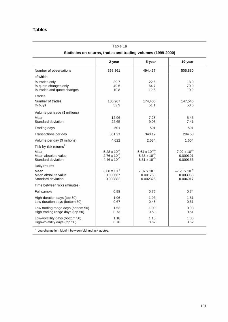
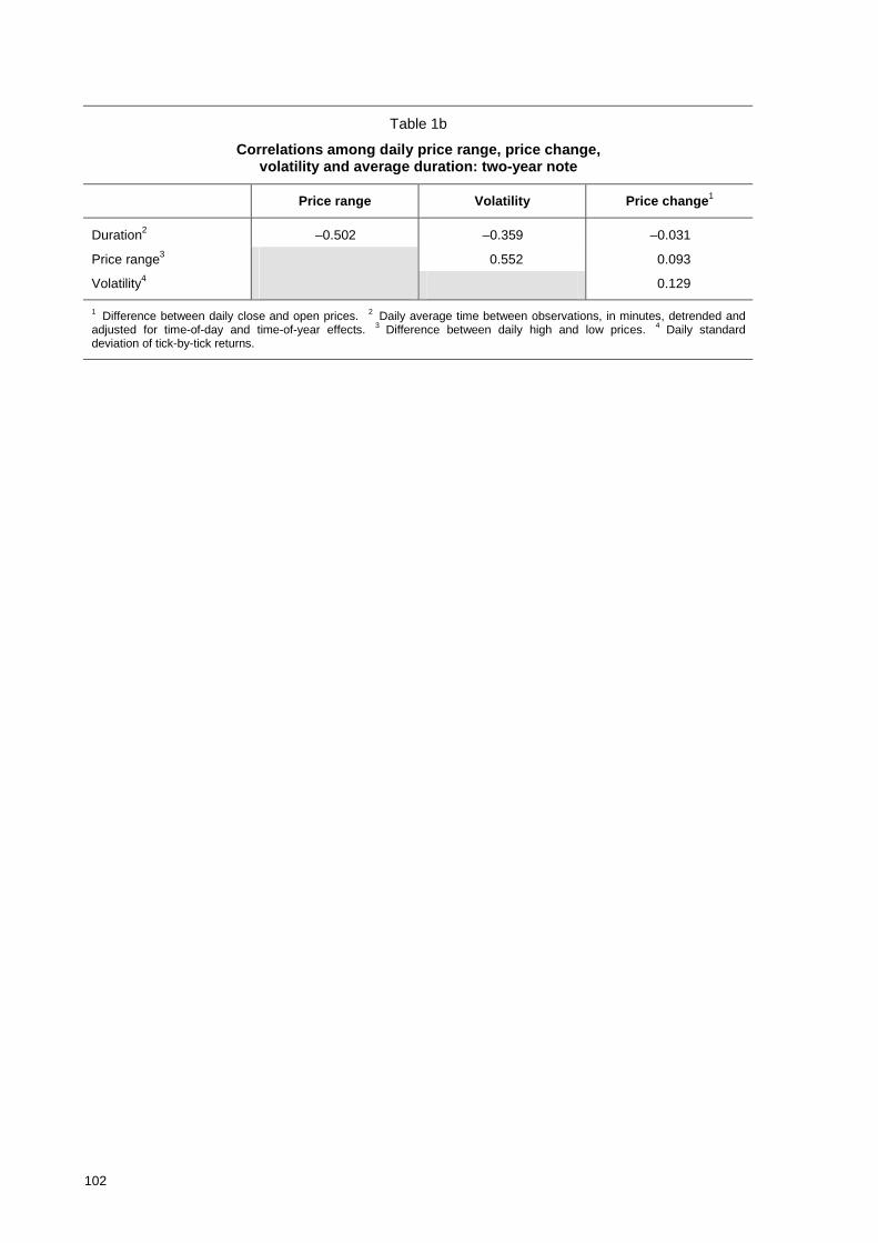

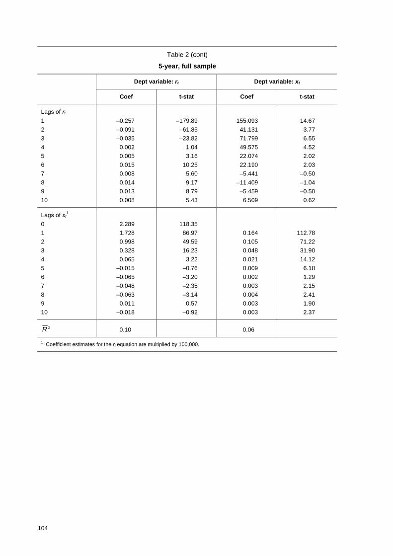
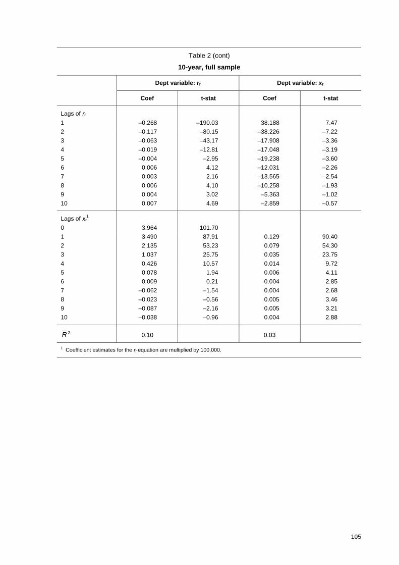
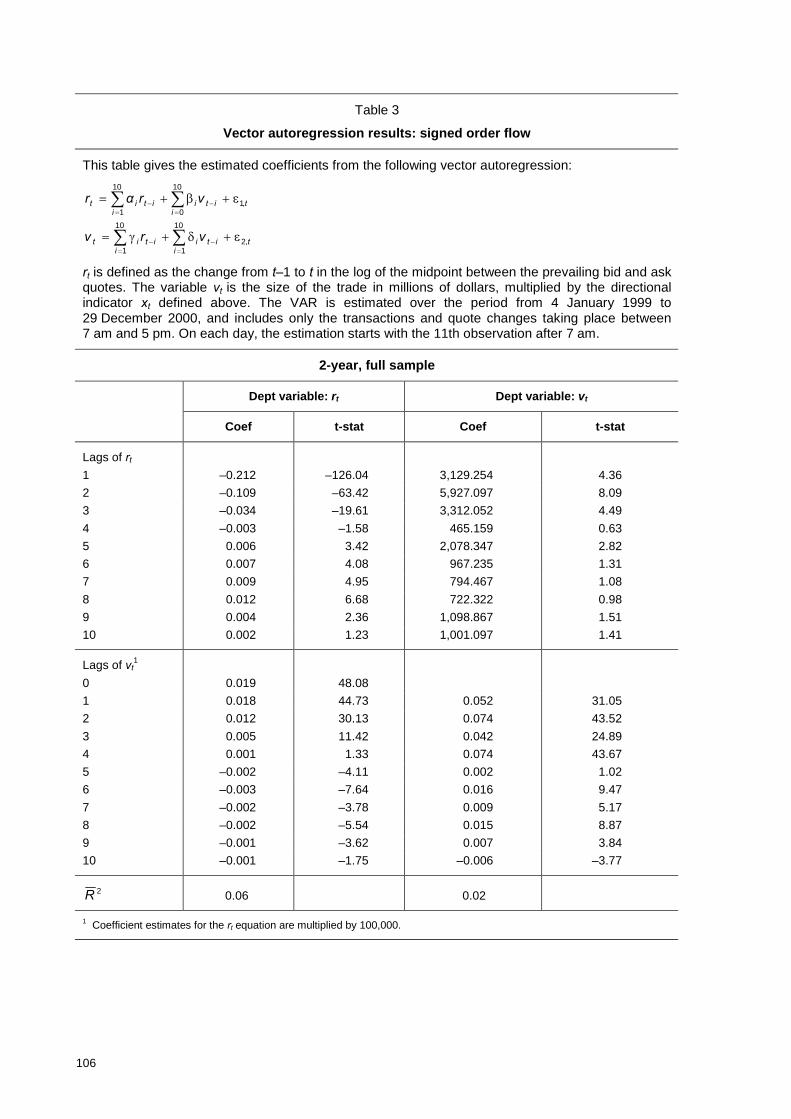

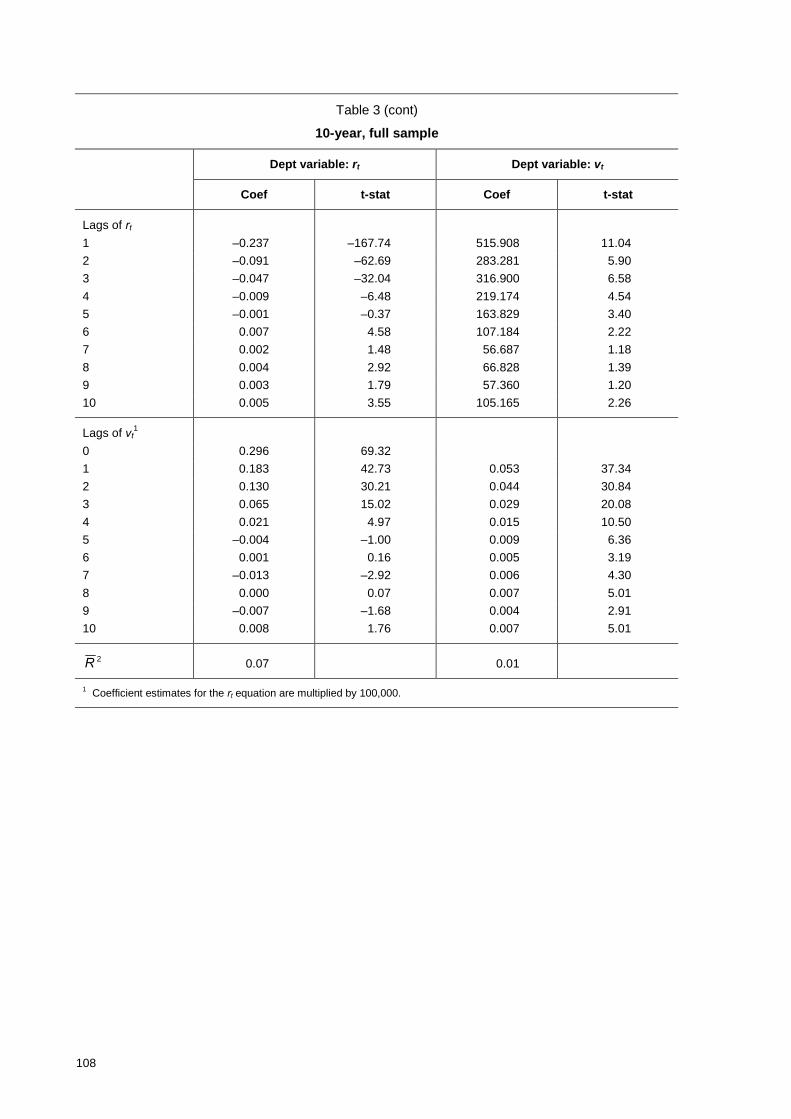


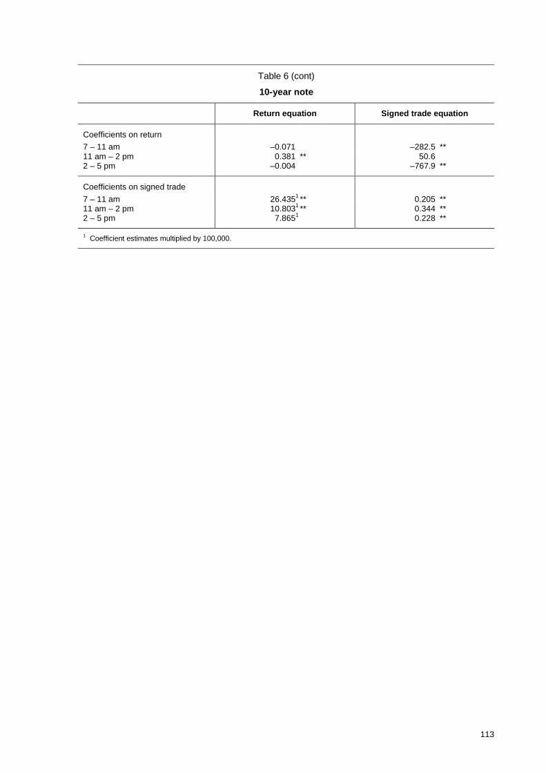


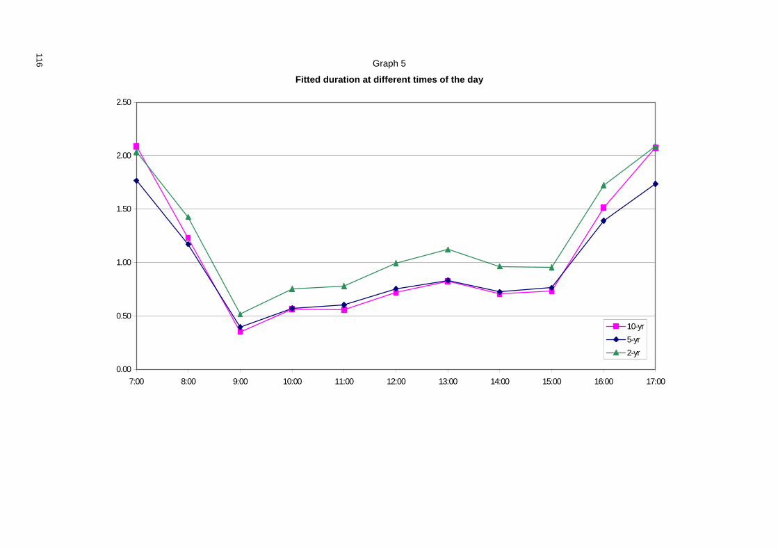
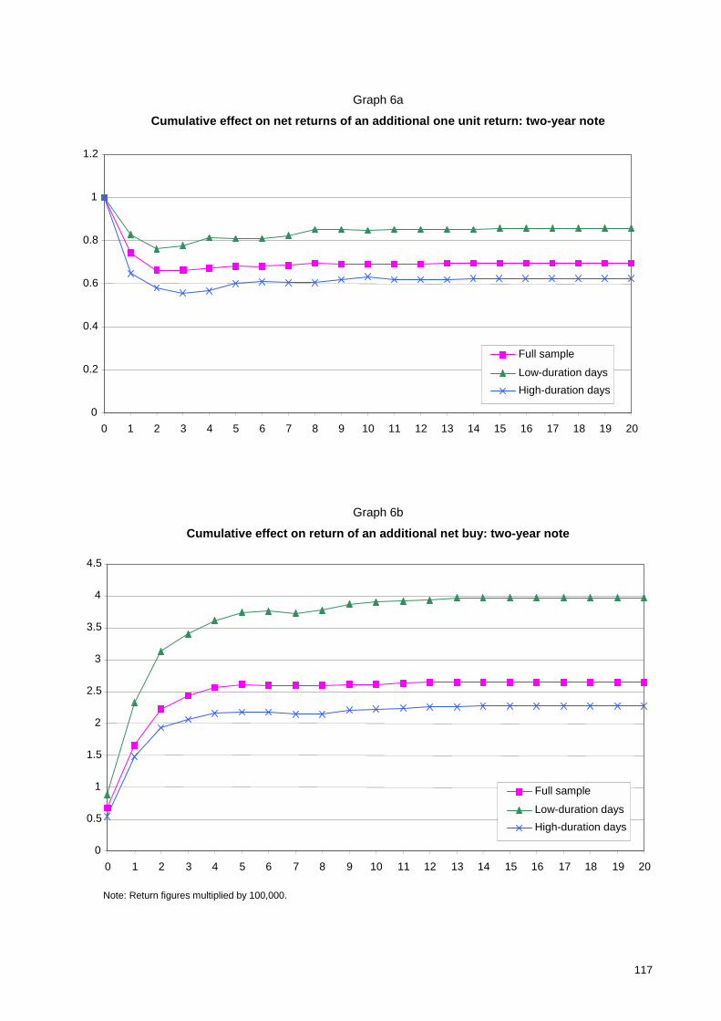
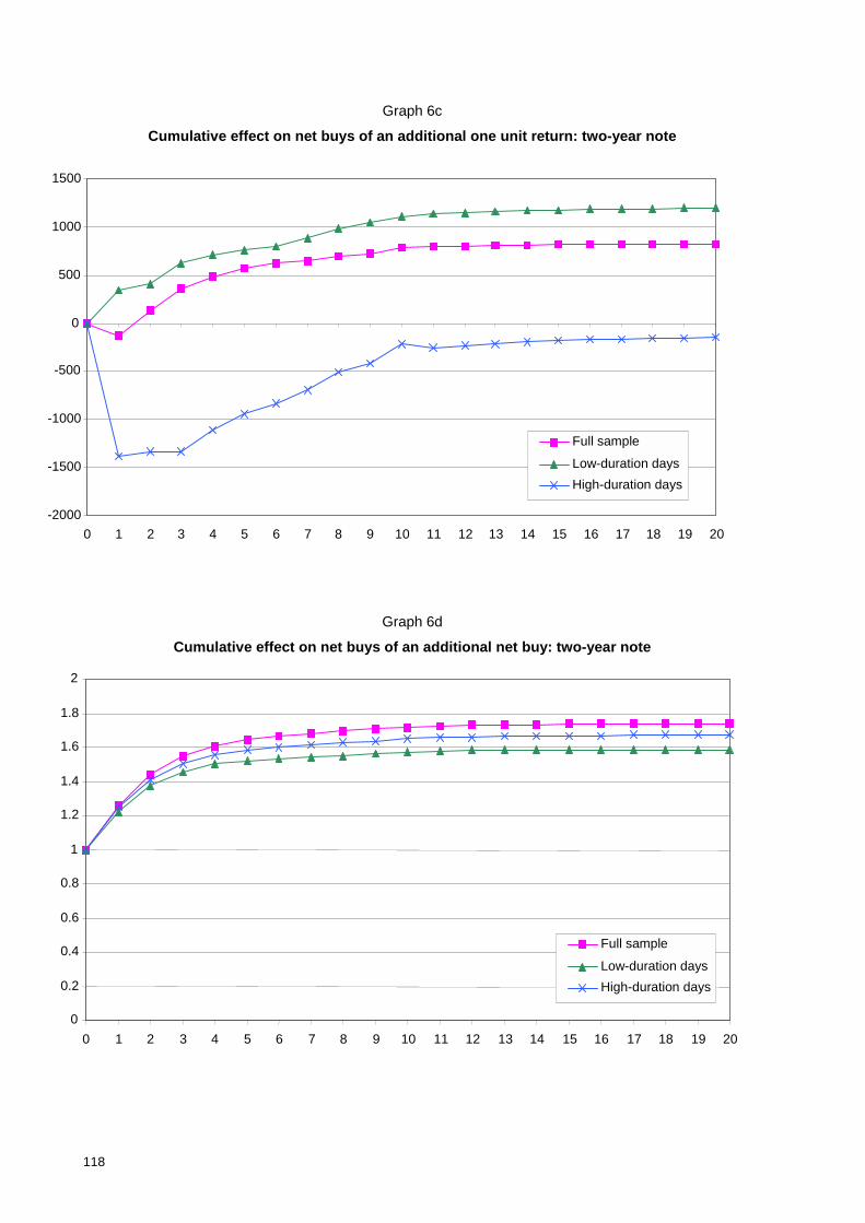
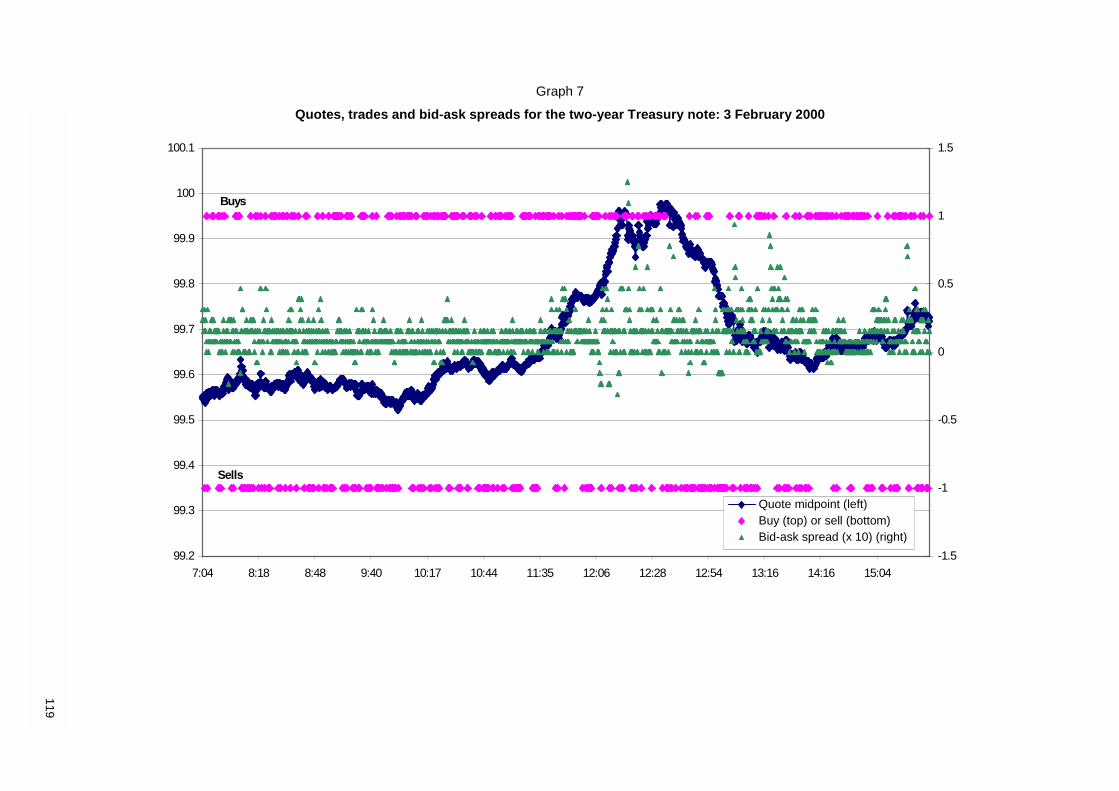
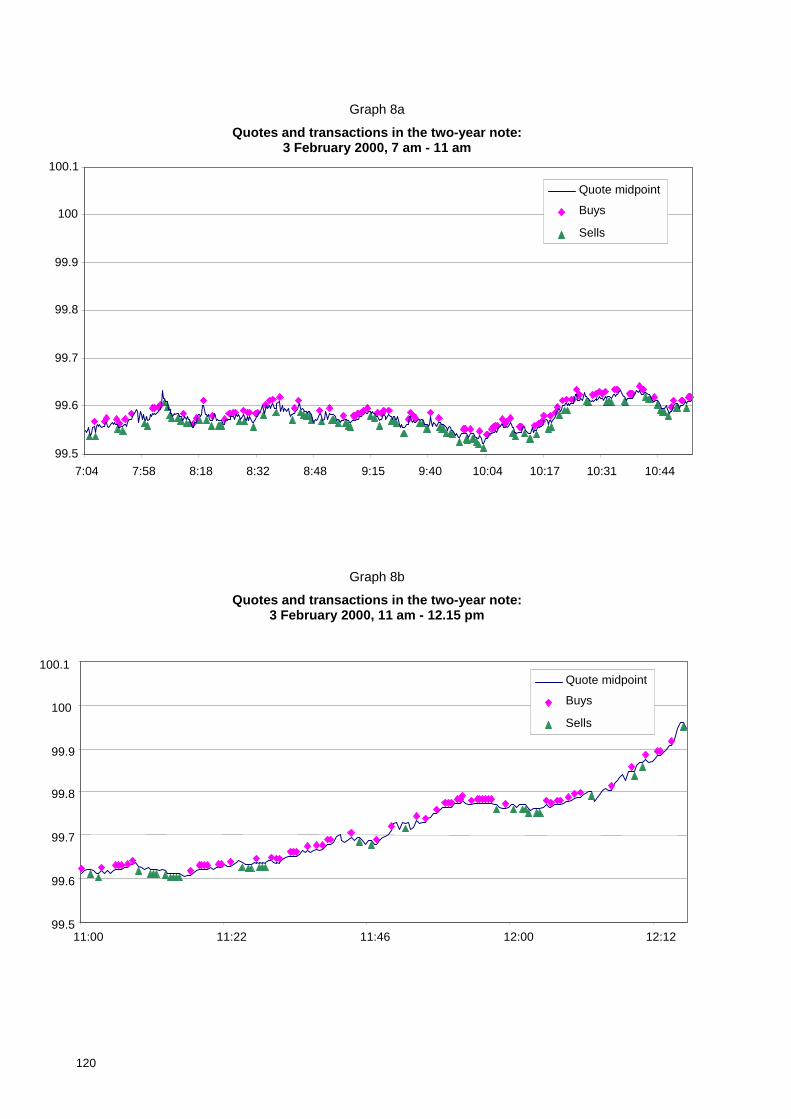
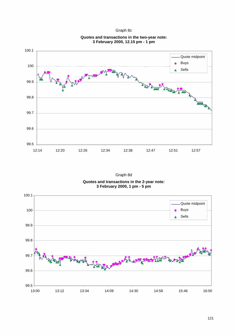


![POSITIVE AND NEGATIVE FEEDBACK IN POLITICS[ Positive and Negative Feedback in Politics ] 5 5 equilibrium. Positive and negative feedback processes lead alternately to the creation,](https://static.documents.pub/doc/80x56/5e6fc60d27274a5c975cef86/positive-and-negative-feedback-in-politics-positive-and-negative-feedback-in-politics.jpg)


