POSSESSION VERSUS POSITION: STRATEGIC EVALUATION IN AFL ABSTRACT In sports like Australian Rules football and soccer, teams must battle to achieve possession of the ball in sufficient space to make optimal use of it. Ultimately the teams need to score, and to do that the ball must be brought into the area in front of goal – the place where the defence usually concentrates on shutting down space and opportunity time. Coaches would like to quantify the trade-offs between contested play in good positions and uncontested play in less promising positions, in order to inform their decision-making about where to put their players, and when to gamble on sending the ball to a contest rather than simply maintain possession. To evaluate football strategies, Champion Data collected the on-ground locations of all 350,000 possessions and stoppages in two seasons of AFL (2004, 2005). By following each chain of play through to the next score, we can now reliably estimate the scoreboard “equity” of possessing the ball at any location, and measure the effect of having sufficient time to dispose of it effectively. As expected, winning the ball under physical pressure (through a “hard ball get”) is far more difficult to convert into a score than winning it via a mark. We also analyse some equity gradients to show how getting the ball 20 metres closer to goal is much more important in certain areas of the ground than in others. We conclude by looking at the choices faced by players in possession wanting to maximise their likelihood of success. KEY WORDS Notational Analysis, Australian Rules Football, Tactical Coaching INTRODUCTION Australian Rules Football (informally known as “AFL” after the Australian Football League) is played with an oval ball on an oval field at high speed, leading to it sometimes being called “What Rules?” by the unschooled observer. Compared to more structured football codes such as American football or rugby league where a “phase of play” always starts in a simply- defined formation, the free-flowing nature of Australian football creates extra dimensions for analysis. This paper describes the qualitative framework for evaluating the phases of AFL and presents empirical interpretation of data from the 2004 and 2005 seasons. AFL coaches are clamouring for this sort of analysis to inform their strategies and training procedures. They know that being in possession of the ball is important, but this research can show exactly how much it’s worth on the scoreboard to take a contested mark, compared with someone from the opposition grabbing the loose ball spilled from the pack. They also know that position is important. They must create opportunities in positions near goal, but their players often have to choose whether to aim at a riskier proposition close to the goalmouth or maintain possession in a worse position. Dynamic programming based on empirically derived parameters can answer this dilemma. Dynamic programming was first applied to AFL (Clarke and Norman, 1998) to answer the question of whether players should concede a point on the scoreboard in order to gain clean possession afterwards. A thesis (Forbes, 2006) based on Champion Data’s statistics uses a Markov model approach to map out the probabilities of transitions between AFL’s phases to predict scoreboard results.
Transcript
POSSESSION VERSUS POSITION: STRATEGIC EVALUATION IN AFL
ABSTRACT
In sports like Australian Rules football and soccer, teams must battle to achieve possession of
the ball in sufficient space to make optimal use of it. Ultimately the teams need to score, and
to do that the ball must be brought into the area in front of goal – the place where the defence
usually concentrates on shutting down space and opportunity time. Coaches would like to
quantify the trade-offs between contested play in good positions and uncontested play in less
promising positions, in order to inform their decision-making about where to put their
players, and when to gamble on sending the ball to a contest rather than simply maintain
possession.
To evaluate football strategies, Champion Data collected the on-ground locations of all
350,000 possessions and stoppages in two seasons of AFL (2004, 2005). By following each
chain of play through to the next score, we can now reliably estimate the scoreboard “equity”
of possessing the ball at any location, and measure the effect of having sufficient time to
dispose of it effectively. As expected, winning the ball under physical pressure (through a
“hard ball get”) is far more difficult to convert into a score than winning it via a mark. We
also analyse some equity gradients to show how getting the ball 20 metres closer to goal is
much more important in certain areas of the ground than in others. We conclude by looking at
the choices faced by players in possession wanting to maximise their likelihood of success.
KEY WORDS
Notational Analysis, Australian Rules Football, Tactical Coaching
INTRODUCTION
Australian Rules Football (informally known as “AFL” after the Australian Football League)
is played with an oval ball on an oval field at high speed, leading to it sometimes being called
“What Rules?” by the unschooled observer. Compared to more structured football codes such
as American football or rugby league where a “phase of play” always starts in a simply-
defined formation, the free-flowing nature of Australian football creates extra dimensions for
analysis. This paper describes the qualitative framework for evaluating the phases of AFL
and presents empirical interpretation of data from the 2004 and 2005 seasons.
AFL coaches are clamouring for this sort of analysis to inform their strategies and training
procedures. They know that being in possession of the ball is important, but this research can
show exactly how much it’s worth on the scoreboard to take a contested mark, compared with
someone from the opposition grabbing the loose ball spilled from the pack. They also know
that position is important. They must create opportunities in positions near goal, but their
players often have to choose whether to aim at a riskier proposition close to the goalmouth or
maintain possession in a worse position. Dynamic programming based on empirically derived
parameters can answer this dilemma.
Dynamic programming was first applied to AFL (Clarke and Norman, 1998) to answer the
question of whether players should concede a point on the scoreboard in order to gain clean
possession afterwards. A thesis (Forbes, 2006) based on Champion Data’s statistics uses a
Markov model approach to map out the probabilities of transitions between AFL’s phases to
predict scoreboard results.
American football, where position is effectively one-dimensional and there are only four
phases – the “downs” – has been analysed using dynamic programming in a famous paper
(Romer, 2002), and a rating system (Schatz, 2005) called DVOA (Defence-adjusted Value
Over Average) evaluates actions with respect to a model of scoreboard value similar to the
one created in this paper. The fast-flowing and open sport of ice hockey has recently been
modelled using a “semi-Markov” approach (Thomas, 2006).
The modelling undertaken here is largely exploratory – this is a mass of new data which
requires further detailed research.
METHODS
Match Equity and Field Equity
Various authors have employed a plethora of terms to describe the expected value of actions
on sporting fields. Studeman (2004) describes the repeated reïnvention and relabelling of
“Win Probability Added” in baseball. Bennett (2005) has a good simple description of how to
value an action that alters the probability of winning the match.
The terminology we use in this paper is derived from the theory of backgammon (Keith,
1996), a game in which the players compete to win points, the first to n points winning the
match. We assume teams of equal strength, although much of the reasoning below is still
valid for uneven teams. Match Equity is the probability of the team to win the match from
this moment, or more specifically:
10
2
1),,,(
≤≤
+=
M
drawwinM
E
pptmE ϕx (1)
The Match Equities of each team in the contest sum to one. A team is always aiming to
increase its Match Equity until it reaches one – certain victory. I.e., it is looking for actions
which maximise ∆EM, or at the very least have ∆EM ≥ 0. As noted in Equation 1, Match
Equity is a function of four parameters:
• the score margin, m
• the time remaining in the match, t
• the position on the field, x
• the possession state or phase of play, ϕ
AFL typically has about 50 scores in a match of 80 live minutes. We define styp as the typical
score of a game (in AFL’s case, the goal worth 6 points is dominant), and ttyp as the typical
time between scores (approximately 100 seconds in AFL). We can roughly decouple the first
two parameters from the others by noting that if we discard any knowledge of x or ϕ , we can
build a satisfactory model of winning probability based only on the time remaining t and
changes to the margin m. The phase and location information can be treated as a perturbation
of the match-winning probability model EM.
To model the net potential value on the scoreboard of the current state of play, we introduce
Field Equity:
)max()max(
)(),( ,,
iFi
i
ioppiiteamiF
sEs
spspE
≤≤−
−=∑ϕx (2)
where
• si is the value of the ith
type of score
• pi,q is the probability of the next score being of type i by team q
The Field Equities of each team in the contest always sum to zero. The Field Equity
fluctuates as play progresses until either team scores, at which team it precipitates an actual
change to the margin m and EF is reset to zero. AFL has two different restart phases, one
being a centre bounce after a goal (where obviously each team has equal chances and EF = 0),
the other being a kick-in from the goalmouth after a behind. Remarkably, empirical evidence
suggests that the average team has zero residual equity in the behind restart phase (see Table
1 in RESULTS).
Changes to Match Equity, Decoupled
m
E
EtmE
M
FM
∂
∂=Π
∆⋅Π≈∆ ),(),( ϕx
(3)
The “Pressure Factor” multiplier Π is the impact an instantaneous change to the margin
would have on the match-winning chances of the teams. Empirically, kicking the first goal in
an evenly-matched contest increases EM from 0.50 to about 0.56. The decoupling transfers the
potential held in the field position into improved match-winning probability. It allows us to
assume that a team that increases EF to +2 soon after the start of a game increases its match-
winning probability to about 0.52, but if only a quarter of the match is left and m = 0, ∆EF of
+2 could imply ∆EM of +0.04, from 0.50 to 0.54. A detailed formula for Π is beyond the
scope of this paper. Henceforth the term “equity” (E) will refer to Field Equity and we will
assume the time remaining is effectively unlimited.
The decoupling assumption only breaks down when both t and m are of the order of ttyp and
styp respectively – i.e., when the game goes down to the wire, the added quantum of a major
score could be the difference between a win (EM = 1) and a loss (EM = 0), and the time left on
the clock must be considered.
Data Collection
Champion Data has been logging qualitative AFL statistics by computer since 1996. All
statistics are classified live by a caller at the venue, connected by phone to a reviewer
watching a monitor, and a data entry operator. Traditionally, AFL statisticians had only
captured the numbers of kicks, marks, handballs, and scores for each player. The system
introduced in 1996 imposes a structure on the flow of play, so that every disposal or use of
the ball must be preceded by a “possession”.
We need to be able to say which player is in possession, in which circumstances he got the
ball, where he was on the field, how much time he had to think once he got it, a rough idea of
what his options were, which option he chose, and whether he successfully executed his
choice. Each of these events has to be put in context, with respect to what happened before
and after the ball was in his control. The data capture software executes a model of the sport,
which only allows certain events to take place in certain circumstances. Every statistic is
time-coded, and since 2004 all possessions are given a position on the field by an
independent operator whose sole responsibility is to pinpoint the location of the ball on a map
of the field for each of these 1000 data points per match.
Testing has shown that the quantity of statistics for each player is logged at better than 99%
accuracy, time is accurate to within about five seconds, and position to within approximately
5-10 metres.
AFL Phases of Play
Possession of the football has been qualitatively stratified to become the descriptive
framework of AFL’s Phases. Phases of Play with a team in possession include:
• Mark. The player has caught the ball from a kick and according to the rules is entitled
to consider his options without being tackled.
• Handball Receive. The player has received a handball from a teammate, uncontested.
• Loose Ball Get. The ball has indiscriminately spilled loose and a player has been in
the right place to pick it up.
• Hard Ball Get. The player has taken usable possession of the football while under
direct physical pressure from an opponent.
Play can also be in an active neutral phase, after a smother of the ball or a similar random
collision. There are also passive neutral phases where the umpire holds the ball, before
launching it back into play. Lastly there are a couple of set-play phases such as a kick-in after
a behind.
For the purposes of this paper we will consider five Phases of Play, which experience and
analysis have shown cover most important facets of AFL:
• “Set” (approximately 35% of possession is granted this way). A player has taken a
mark or received a free kick, or has been given another set-play role. He has an
optimal amount of time to consider options and make the right choice. We will ignore
kick-ins from goal in this paper.
• “Directed” (approx 38%). The ball was directed into the player’s possession by a
teammate, either via a handball, a kick to the player’s advantage without achieving a
mark, or a knock-on or hit-out intended for the player. Generally the player has space
to run onto the ball and some time to make a good decision.
• “Loose” (approx 17%). The player won a virtually random ball via a loose ball get,
and while he is not yet under physical pressure there is not a lot of time to evaluate the
situation.
• “Hard” (approx 10%). The player won the ball under direct physical pressure and
often must take the quickest option available to avoid being caught with the ball.
• “Umpire”. The umpire has the ball and will restart play with equal chances for both
teams.
We have ignored quasi-possession states like knock-on, hit-out and kick off the ground for
this paper. A full description of Phase of Play would also include extra dimensions such as:
how fast the ball travelled to where it is (catching the defence napping, for instance); who is
currently on the field (is it the best 18 players available?); what formation the team is playing
(flooding the backline to reduce the odds of uncontested ball near the opposition’s goal).
Assumptions
AFL is regularly played at a dozen different venues, each with slight variations from the ideal
oval shape and various lengths and widths. The shortest ground is the SCG at 148.5 metres,
meaning that the 50m-wide centre square touches the 50m arcs at each end of the ground. At
Subiaco in Perth, on the other hand, there are 175.6 metres between the goal-lines and
therefore 12.8 metres of territory between the top of the arc and the centre-square. When
plotting locations, it is important to note that some areas of the ground simply don’t exist at
some grounds, and that the wings are much wider at the SCG (length:width ratio of 1.09:1)
than Geelong (1.47:1).
The positional capture software assumes that every ground is a perfect ellipse, and only the
lengths of the axes vary, so the operators can accurately pinpoint play. For analysis, we use
the MCG (160 × 138 metres) as the standard ground and transform the other venues into this
shape to utilise their data. This transformation preserves fixed areas of the ground such as the
centre-square, boundary and the corridor leading to goal, while distorting distances and
angles in other regions.
We will always show teams attacking the goal to the right of the page. Contour maps have
been generated using ComponentOne Chart3D v8. Other diagrams have been designed by the
author.
An implicit assumption in the equity model is that the expected value of the next score is a
good measure of the current phase of play, no matter how many minutes in the future that
score may be. This has advantages over a Markov Model in that we do not assume that future
states are exactly classifiable, instead there may be subtle repercussions of actions which are
evident further down the track and should not be washed away by repeated normalising.
Coaches value the players who can see three or more moves ahead, and don’t just look for an
easy option in front of them. The disadvantage of the equity approach is that the further we
go from the source phase, the less relevance it has to the developing play, as more
randomness floods in. Standard error measurements are quite high because of the number of
data points ignored.
Method of Calculating Estimated Equity
For each data point, the value of the next score has been noted. This could be +6 (a goal for
this team), +1 (a behind for this team), -1 (a behind for the opposition), or -6 (a goal for the
opposition). Data points are excluded from analysis if there is no further scoring in the
quarter. An example appears in Tables 1 and 2 at the start of the RESULTS section below.
It has been assumed that left/right and north/south biases are inconsequential, so the standard
ground has been folded down the spine and data points from each half are analysed together.
We have used two different positional filters in this paper. The contour graphs are generated
using a six metre square grid. All points within a six metre radius of the vertex are taken into
account in the calculation, meaning that each point appears in roughly three map points – this
is an attempt at smoothing, knowing the natural sampling error in the data. Parts of the map
with insufficient data (fewer than ten points in the disc or an equity standard error of greater
than 0.5) are shown blank.
Where we want to measure true statistical deviations and start to develop a model, the zones
must not overlap. The semi-ellipse (remembering that the ground has been folded along its
spine) is divided into 200 zones of equal area. First the length-wise (X) axis is divided into 25
sections to segment the ellipse into 25 equal areas. Then seven curves are drawn equidistant
from each other, between the spine and the boundary to cut each strip into eight zones.
Error figures presented are two standard errors (95% confidence) except where noted.
RESULTS
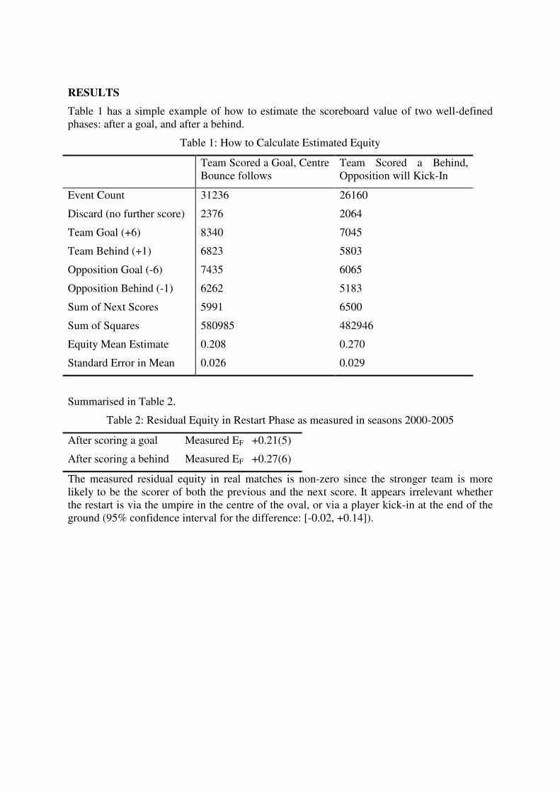
Table 1 has a simple example of how to estimate the scoreboard value of two well-defined
phases: after a goal, and after a behind.
Table 1: How to Calculate Estimated Equity
Team Scored a Goal, Centre
Bounce follows
Team Scored a Behind,
Opposition will Kick-In
Event Count 31236 26160
Discard (no further score) 2376 2064
Team Goal (+6) 8340 7045
Team Behind (+1) 6823 5803
Opposition Goal (-6) 7435 6065
Opposition Behind (-1) 6262 5183
Sum of Next Scores 5991 6500
Sum of Squares 580985 482946
Equity Mean Estimate 0.208 0.270
Standard Error in Mean 0.026 0.029
Summarised in Table 2.
Table 2: Residual Equity in Restart Phase as measured in seasons 2000-2005
After scoring a goal Measured EF +0.21(5)
After scoring a behind Measured EF +0.27(6)
The measured residual equity in real matches is non-zero since the stronger team is more
likely to be the scorer of both the previous and the next score. It appears irrelevant whether
the restart is via the umpire in the centre of the oval, or via a player kick-in at the end of the
ground (95% confidence interval for the difference: [-0.02, +0.14]).
Equity Maps
Figure 1: “Set” Phase Contour Map
The value of taking a mark and having a set shot at goal directly in front can be seen in this
map, with an expected value of more than four points extending all the way out to about 40
metres from goal. A free kick within 25 metres makes the goal a virtual certainty. The tight
bunching of contour lines from 40 to 60 metres out along the spine shows the natural limit of
an AFL footballer’s kick, being about 50-55 metres. To get within one kick of goal, and have
the time to execute it, is extremely valuable.
Figure 2: “Directed” Phase Contour Map
Figure 3: “Hard” Phase Contour Map
“Directed” (Figure 2) is the second-best phase for a footballer to receive the ball in. Usually
he has received a handball in some space and should be able to execute his preferred option.
But often he will have to take critical time to swivel as the defence closes in, and it’s only
within ten metres of goal that the maximum six points can almost be assumed. The gradient
we saw at 40-60 metres in Figure 1 is completely missing here, showing the greater difficulty
of a snap shot on the run – the attacker wants to be within 30 metres.
An utterly different picture (Figure 3) awaits the player who faces the extreme pressure of a
hard ball get. Even within ten metres of goal the expected scoreboard outcome is just 3.5
points. Equity is below zero for the entire defensive zone, but interestingly there is a peak at
the top of the forward arc, indicating that perhaps this is one place on the ground where he
has two reasonable areas either side of him to shoot out a handball and find a teammate who
suddenly has options within range of goal. This circumstance often happens after the centre
bounce when a quick kick lands at the congested top of the arc with the opposition still
rushing the centre square.
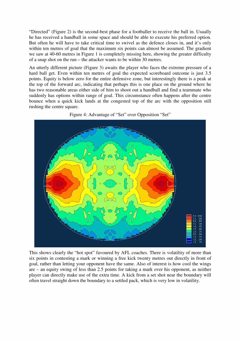
Figure 4: Advantage of “Set” over Opposition “Set”
This shows clearly the “hot spot” favoured by AFL coaches. There is volatility of more than
six points in contesting a mark or winning a free kick twenty metres out directly in front of
goal, rather than letting your opponent have the same. Also of interest is how cool the wings
are – an equity swing of less than 2.5 points for taking a mark over his opponent, as neither
player can directly make use of the extra time. A kick from a set shot near the boundary will
often travel straight down the boundary to a settled pack, which is very low in volatility.
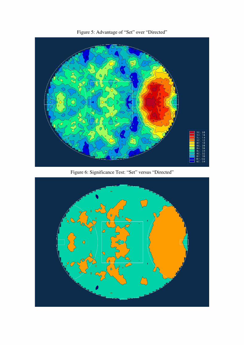
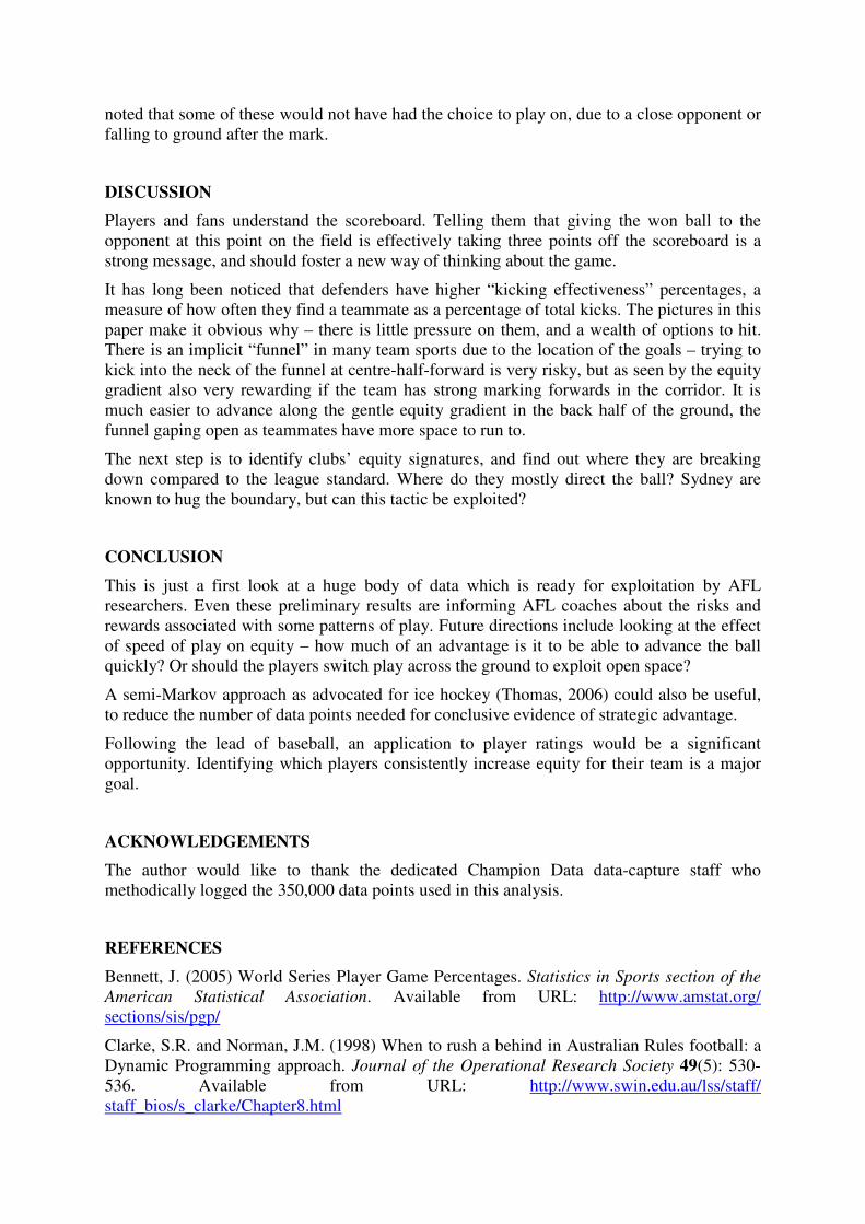
Figure 5: Advantage of “Set” over “Directed”
Figure 6: Significance Test: “Set” versus “Directed”
Calculated as an average over the ground, there is only a boost of 0.3 points to be gained by
taking a mark instead of receiving a handball. In modern football uncontested marks across
the half-back-line are cheap, with the opponent barely interested in forcing the man to go
back and take the set shot. But the advantage is wholly concentrated in the forward-50 arc,
with an extra 1.5 points available on the scoreboard for having a set shot rather than a running
shot at goal between 25 and 45 metres out.
The light areas on Figure 6 show the regions where it is significantly better, at the two-sigma
level, for a player to take a mark rather than gather it uncontested.
Average Phase Equity
The mean net value of each of the phases was calculated by averaging over the 200 zones on
the field. This works as a “standard candle” to investigate deviations by teams or in certain
situations.
Table 3: Equity of Possession Phases, Averaged Over Field
Phase Mean Equity Comments
Set +1.61(2) Being awarded a free kick in the centre circle is worth more
than 1½ points on the scoreboard
Directed +1.32(2) About half-way between Loose and Set, this Phase tends to
show up the good decision makers
Loose +1.11(2) Even if the options aren’t great, it’s still worth more than
two points on the scoreboard to be in the right place instead
of his opponent
Hard +0.80(3) Half the value of a set shot, compared to a 50/50 Phase
A Player’s Choices: What Happens Next
Imagine a player who has just taken a mark 70 metres out from goal, on about a 40°-45°
angle. It’s unlikely he can score himself, and he faces an unenviable choice between bombing
it long in hope of improved field position without turning the ball over, or picking out a
nearby teammate to do the dirty work for him. This scenario – within six metres – has played
out 822 times over the seasons 2004-2005. On average, a team in this position can expect to
convert to about two points on the scoreboard (2.06(14)).
It’s immediately obvious from Figure 7 below that if the player passes short and keeps it near
the boundary, he almost always finds a teammate. Even more encouragingly, the team scores
from there virtually every time. On the other hand, directing the ball long into the central
corridor seems to be about a 50/50 proposition to hold onto the ball. Is it worth the risk? And
should he play on, relinquishing the set shot time to gain some ground by running?
Figure 7: Mark on the MCG Half-Forward Flank
Figure 7 shows the results
of the 195 marks at the
MCG from this position.
Showing all venues made
the picture too crowded.
The grey speckle in the
lower left is the collection
of points where a player
marked. The plus signs (+)
show where he managed to
get the ball to a teammate,
while the red squares are
immediate turnovers. The
grey circles indicate the
ball went into the umpire’s
control. A ring around the
marker means that the next
score was to the opposition
– no ring indicates a score
for the marking player’s
team. The nine diagonal
slashes are the rare
occasions that the player
managed to run to this
point and scored for
himself.
Table 4: Choices from a Mark (All Venues), 70 metres out on a 40-45 degree angle