1 POST-PROCESSING POULIQUEN ECHO CORRECTION FOR SEABOTTOM CLASSIFICATION Daniel Rodríguez-Pérez 1 , Noela Sánchez-Carnero 2 , Juan Freire 3 1 Departamento de Física Matemática y de Fluidos, Facultad de Ciencias, UNED. Madrid (Spain) [email protected]2 Grupo de Recursos Marinos y Pesquerías, Facultad de Ciencias, Universidade da Coruña (Spain) [email protected]3 Barrabes-Next, Madrid (Spain) [email protected]Abstract One of the unsolved problems in seabed classification is echo correction, aimed at presenting all the pings in a standardized form to readily compare them to each other. After correction the echoes from the same bottom type would look the same, independent of the particular bottom depth. Based on a diffuse reflection model, Pouliquen suggested in 2004 to acquire the echoes scaling pulse lengths proportionally with depth. In this work, we recover Pouliquen’s idea to apply it during post- processing. The signal of a single-beam echosounder is time and power adjusted, and then convolved with a structure element simulating the loss of resolution of the signal at a smaller reference depth. The resulting depth correction is consistent for sandy and muddy bottoms between 5 and 40 m deep. The results of testing this method are shown for the Ría de Cedeira (in Galicia, northwest of Spain). The results of the final classification are compared with those obtained from direct observations and from interviews with local fishermen. Keywords: Pouliquen depth correction; seabed classification; aggregative clustering. PACS no. 43.30.Gv, 43.30.Hw 1 Introduction Acoustic methods have been broadly used for sea-bottom classification [1], in particular single-beam scientific echosounders calibrated to provide accurate scattering strength measures [2], time responses [3]) and echo shape features (moments, wavelet coefficients, fractal dimension, etc.) [4, 5] that have been related to different seabed types within a study area. To classify the seabed from its acoustic response, the different responses from the different sea-beds characterized by the echo shape and amplitude (that depend mostly on the sea bottom depth) have to be made comparable. This first step is called correction and
Transcript
1
POST-PROCESSING POULIQUEN ECHO CORRECTION FOR
SEABOTTOM CLASSIFICATION
Daniel Rodríguez-Pérez1, Noela Sánchez-Carnero
2, Juan Freire
3
1 Departamento de Física Matemática y de Fluidos, Facultad de Ciencias, UNED. Madrid (Spain)
[email protected] 2 Grupo de Recursos Marinos y Pesquerías, Facultad de Ciencias, Universidade da Coruña (Spain)
Acoustic methods have been broadly used for sea-bottom classification [1], in particular
single-beam scientific echosounders calibrated to provide accurate scattering strength
measures [2], time responses [3]) and echo shape features (moments, wavelet coefficients,
fractal dimension, etc.) [4, 5] that have been related to different seabed types within a study
area.
To classify the seabed from its acoustic response, the different responses from the different
sea-beds characterized by the echo shape and amplitude (that depend mostly on the sea
bottom depth) have to be made comparable. This first step is called correction and
Rodríguez-Pérez, D., Sánchez-Carnero, N., Freire, J.
2
compensates the power losses (power correction) and the temporal distortion (time correction)
of the received echoes. The objective of this work is to improve this latter correction, which is
the most important in zones with depth varying rapidly such as coastal areas.
A vertical single-beam echosounder (VBES) produces acoustic waves that propagate with
spherical symmetry from its transducer, traveling at the speed of sound in water, c≈1500 m/s.
The larger part of the emitted power (up to 94% for a 7ο wide Gaussian beam, corresponding
to a maximum directivity of 28 dB) will be directed along the main lobe of the directivity
pattern. The emitted power lasts for a small time τ leading to a pulse length of l=cτ. The wave packet reaches the bottom and the sub-bottom region beneath and is reflected and
backscattered to the transducer, which samples the incoming wave pressure (averaged out to
intensity) in sampling time bins of duration δt (usually, δt= 1
4τ).
The total reflected power follows the sonar equation, that adds a range R dependency caused
by the wave spherical spreading, −20×log10
R (for the total echo energy), and the wave
attenuation in water, −2αwR. The correction terms regarding the acoustic intensity, depending
not only on depth, but also on time after the first bounce instant t0, are not so easily calculated
due to the finite pulse length that does not usually scale with depth (power correction would
be much easier in this case, as proposed in [6]). As the acoustic wave spreads out, the lateral
parts of the main acoustic lobe, and the side-lobes of the acoustic directivity pattern, will add
up to form the tail of the received ping and, for shallow depths or large pulse lengths, the
former lateral lobes may become indistinguishable from the main one. The signal reflected
from lobes further apart than 60ο from the central lobe will not be observable with a VBES
kept at the water surface, as it will become mixed with the second echo (twice reflected from
the bottom, after an air-water interface reflection).
The objective of this paper is to introduce a ping correction scheme suited to perform
seabed classification in coastal areas with steep depth variations, developing the idea of [6] of
scaling the pulse-length with depth, but instead of modifying the echosounder, simulating this
in post-processing. A physically based classification method (aggregative clustering) will also
be introduced and tested in a study area.
2 Material and methods
In order to perform the sea bottom classification we will classify corrected echoes, thus the
first part of the methodology will consist on echo delimitation and correction from the raw
intensity ping recorded by the digital VBES. Afterwards, in order to interpret this
classification, we will use direct measurements and knowledge of a study area. Finally, we
will refine this seabed classification.
Post-processing Pouliquen echo correction for bottom classification
3
2.1 Echo delimitation and correction
Bottom detection is necessary to time align pings and to compute echo duration. We will use
a thresholding algorithm for this: the beginning of ping first bounce will be located at the bin
previous to the ping maximum which lays at less than 40 dB below that maximum; the end of
that first bounce will be determined geometrically, at twice the distance from the surface as
the bottom position is (the echosounder is kept right below the water surface). The 40 dB
threshold was determined empirically, and may change for other echosounders or sea-water
conditions or depth ranges.
The time correction of the echoes was performed in two steps. First, a deep enough depth
R0 was chosen, large compared to the depths found in the survey (we have chosen 40 m).
Then all the echoes were stretched (interpolated) to fit within 2R0/(cδt) bins to provide the
simplest time correction. Then the power correction was applied adding to each normalized
ping 30 log10(R/Rref) [7], where Rref is the reference depth for the correction.
As suggested by Pouliquen in [6], the finite ping length τ requires further adjustments of this time correction. In particular, Pouliquen suggests to use depth dependent emitted pulses
with lengths τ(R)=(R/R0)τ0, i.e., shorter, the shallower. Our approach will be to simulate a
lengthening of the pulses of the deeper pings, i.e., we will apply a ping-lengthening Pouliquen
correction (PLP).
We first observe that ping intensity I(t) can be computed as the convolution of the emitted
pulse W(t) with a time- (t) and depth- (d) dependent bottom response function G(ct/d) [8].
Then, to simulate the PLP from a deep zone (R1), we may convolve the ping intensity I(t) with
a properly chosen structure element W(d,t), so that the resulting time-normalized ping
resembles one measured at a shallower bottom (Rref < R1). If the pulse length of the Rref deep
ping is τref=τ, then, the Pouliquen’s suggested ping length for the R1 ping would be
τ1=(R1/Rref)τref, that is the simulated pulse length has to be lengthened by ∆τ1=τ1-τref. This lengthening will be simulated here using as the structure element W(d,t), a rectangular pulse
function ∆τ1 long and 1/∆τ1 high (for energy conservation) which does not render the exact result, but is numerically convenient (see figure 1).
Figure 1: Ping correction: time correction and ping widening convolution.
Rodríguez-Pérez, D., Sánchez-Carnero, N., Freire, J.
4
2.2 Study area
The study area was the Ría de Cedeira, one of the smallest ones in the Galician coast (693 ha).
This area has a high diversity of bottom substrate types and topographic features including a
subarea with high slope (up to 20ο in rocky area and up to 6ο in sandy area) where the bottom
attains large depths (50 m), and also a flat shallow area (<10 m), containing rocky, sandy and
muddy bottoms [9].
Figure 3: Study area showing bathymetry and acoustic transects.
The acoustic survey was carried out from 3rd to 6th May 2008 with good weather
conditions. A total of 62 acoustic transects were performed covering the total of the Ría (see
figure 3). Acoustic data were recorded with a single-beam echosounder (EA400P Simrad)
working with a 38/200 kHz transducer. This transducer was attached to the hull rail of a small
boat (6.95 m). The 200 kHz and 38 kHz frequencies were operated with a pulse length of
256 µs and 1024 µs, respectively. Both frequencies worked with a maximum emitting power (1 kW) and a sampling rate of 1 ping/s. The boat speed was kept between 4 and 4.5 knots.
Post-processing Pouliquen echo correction for bottom classification
5
2.3 Classification
Prior to classification, and in order to reduce the number of samples in the classification and
also to reduce the inter-ping variability, corrected echoes were averaged, taking one every 10
pings. The ping average was computed selecting from the 21 neighboring pings (10 before
and 10 after) those 10 bearing the least differences among them. The location of that average
ping was taken at the centroid of the 21 ping locations. This leaves a number of N0 echo
representatives to be further classified. In our case, N0=4663 representatives.
Here, and in what follows, we compare the pings using their intensity level, measured in
dB (the usual visual representation); this allows us to extend the comparison outside the main
lobe high intensity response into the ping tail. Then, we will combine (average) the ping’s
linear intensity (in Watts/m2) to obtain the representative echoes, because this operation is
physically meaningful. The classification of the remaining representative echoes was
performed using a two-step hierarchical clustering algorithm.
In the first step a number N1 of target classes covering a fraction f1 of the total N0
representatives is specified. Starting from the N0 representative echoes, every contiguous pair
was compared (in dB) and the pair with the least difference was combined (averaged in linear
scale) in one representative (descendent) echo, thus effectively enlarging the length of the
representative echoes corresponding to the same type of echo response. This is iterated until
the N1 representatives representing the largest number of original pings, cover a fraction f1 of
the entire sample set. In our case, we have retained N1=500 representatives, covering f1=90%
of the sampled transects.
The second step is similar to the first one, prescribing N2 target classes covering a fraction
f2 of the N0 representatives. However, the echo comparison is extended to all of the possible
pairs in the N1 representatives obtained in the previous step, and not only to the contiguous
ones. In our study area we selected, N2=10 and f2=95%.
To assess the robustness of the classification, the class representatives (corrected pings
averaged over each class) of the 5 largest classes were used to reclassify, by minimum
distance, all the N0 representatives. The resulting reclassification should keep the spatial
coherence of the previous one, while reducing the “inertia” (mixtures of two similar classes
appearing one after another along a transect) induced by the first step.
2.4 Groundtruthing
To validate the acoustic classification a thematic map of the Ria de Cedeira developed
through interviews with local fishermen was used. The geographical accuracy of the map is,
nevertheless, approximate but the bottom types are expected to fit within a reasonable range
of the actual ones. Furthermore, the spatial coherence of the classification obtained will allow
interpreting the classes obtained in terms of the fishermen seabed classes.
Rodríguez-Pérez, D., Sánchez-Carnero, N., Freire, J.
6
3 Results
The PLP correction applied to the pings brings all the pings of the same seabed type to the
same depth-normalized form (within the experimental error). Figures 3a,b show first bounces
of pings (38 kHz signal) corresponding to fine sand (the most abundant in the study area)
measured at different depths after time-stretching only and after applying the PLP correction.
(a) (b)
Figure 3: Time stretched (a) and PLP corrected (b) first echoes corresponding to fine sand
bottom measured at different depths.
The ping representatives of the 5 largest classes obtained from the 200 kHz and 38 kHz
signals are shown in figure 4. The two lower intensity echoes (yellow and green) are
interpreted as sandy or muddy flat bottoms. The next two (red and orange) seem like medium
and coarse sand. The highest intensity and widest echo (brown) corresponds to rocky bottoms.
(a) (b)
Figure 4: Echo representatives of the 5 largest classes of the (a) 200 kHz and (b) 38 kHz
classifications.
Post-processing Pouliquen echo correction for bottom classification
7
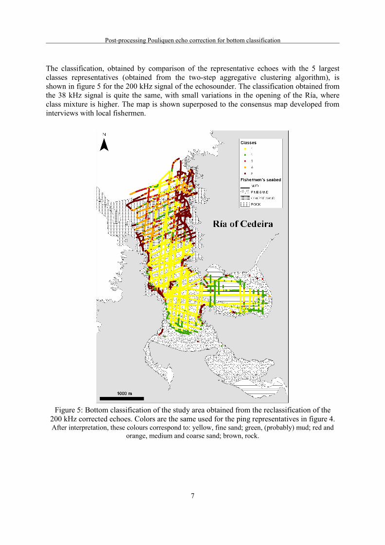
The classification, obtained by comparison of the representative echoes with the 5 largest
classes representatives (obtained from the two-step aggregative clustering algorithm), is
shown in figure 5 for the 200 kHz signal of the echosounder. The classification obtained from
the 38 kHz signal is quite the same, with small variations in the opening of the Ría, where
class mixture is higher. The map is shown superposed to the consensus map developed from
interviews with local fishermen.
Figure 5: Bottom classification of the study area obtained from the reclassification of the
200 kHz corrected echoes. Colors are the same used for the ping representatives in figure 4. After interpretation, these colours correspond to: yellow, fine sand; green, (probably) mud; red and
orange, medium and coarse sand; brown, rock.
Rodríguez-Pérez, D., Sánchez-Carnero, N., Freire, J.
8
4 Discusion and conclusions
The PLP correction introduced in this paper is well suited to correct pings measured in
shallow waters, allowing to obtain a successful bottom classification of a coastal zone with
depths as shallow as 5 m over extended areas and as deep as 35−40 m (figure 3). The aggregation clustering method used for the classification is (thanks to the PLP
correction applied) a physically consistent method, as it builds up on averaging the intensity
measurements in acoustically close resembling bottoms. This would be equivalent to the large
averages, of over 100 pings, used in oceanographic surveys covering more extended areas.
Moreover, the observed dispersion around the “average ping” thus computed, lies within the
bounds expected from the speckle distribution in soft bottoms, being larger in rough (rocky)
bottoms.
In the classification obtained, the rocky bottoms of the coast reefs are clearly detected.
They correspond to higher normalized intensity pings with longer echoes. The different types
of rocky bottoms can be differentiated keeping more classes, although fast changes in rocky
bottoms cause high class mixture. The coarse sand and the fine sand are well differentiated
from their echo normalized intensity. However, in the case of muddy bottoms, mostly located
in the shallower inlet to the east, their echo shapes are almost the same as fine sand and it is
difficult to say where one class changes to other but for the differences, mostly in the average
intensity in different parts of the echo tail. These differences may be caused by the different
acoustic angular response of these bottoms, but may also include information about the
irregularities present in them. This problem of granulometry discrimination in sedimentary
bottoms has been also reported by other authors [10, 11].
It is important to point out that seabed types do not appear correlated with depth. For
example, fine sand was found throughout the depth range. Mud was found in the shallower
areas south-east (confirmed by direct observation) and in the south-west of the study area
(near Villarrube’s beach, although its presence was not confirmed by groundtruthing). It also
appears in a deeper region (∼30 m) near the outlet of the Ría, surrounded by rocks and fine sand, a formation common in other Galician Rías [12].
When compared with the fishermen map, the qualitative agreement of the interpolated map
is good, although the boundaries of the seabed covertures are not so accurate and the amount
of mud and coarse sand are overestimated by the fishermen with respect to the acoustic
classification. This misadjustment in the class boundaries between both maps may be
explained by an overestimation of the distances closer to the coast by the fishermen, a well
known perception bias [13].
Acknowledgements
The authors wish to acknowledge Prof. M. Mozynsky for enlightening discusion about the ideas in this
paper.
Post-processing Pouliquen echo correction for bottom classification
9
References
[1] A. Kenny, I. Cato, M. Desprez, G. Fader, R. Schüttenhelm, and J. Side. An overview of
seabed-mapping technologies in the context of marine habitat classification. ICES
Journal of Marine Science, 60:411–418, 2003.
[2] H.M. Manik, M. Furusawa, and K. Amakasu. Measurement of sea bottom surface
backscattering strength by quantitative echo sounder. Fisheries Science, 72:503–512,
2006. 10.1111/j.1444-2906.2006.01178.x.
[3] B.R. Biffard, S.F. Boomer, N.R. Chapman, and J.M. Preston. The Role of Echo Duration
in Acoustic Seabed Classification and Characterization. In OCEANS 2010, pages 1–8.
IEEE, 2010. 10.1109/OCEANS.2010.5664480.
[4] J. Tegowski, N. Gorska, and Z. Klusek. Statistical analysis of acoustic echoes from
underwater meadows in the eutrophic Puck Bay (southern Baltic Sea). Aquatic Living
Resources, 16:215–221, 2003.
[5] P.A. vanWalree, J. Tegowski, C. Laban, and D.G. Simons. Acoustic seafloor
discrimination with echo shape parameters: A comparison with the ground truth.