+ All Categories
Home > Documents > POSTEARTHQUAKE REPAIR OF PRECAST CONCRETE COLUMN …

POSTEARTHQUAKE REPAIR OF PRECAST CONCRETE COLUMN …

Date post: 10-Feb-2022
Category:
Upload: others
View: 2 times
Download: 0 times
Share this document with a friend
185
POSTEARTHQUAKE REPAIR OF PRECAST CONCRETE COLUMN-TO-FOOTING PLASTIC HINGES by Dylan Neil Brown A thesis submitted to the faculty of The University of Utah in partial fulfillment of the requirements for the degree of Master of Science Department of Civil and Environmental Engineering The University of Utah August 2014
Transcript

POSTEARTHQUAKE REPAIR OF PRECAST CONCRETE

COLUMN-TO-FOOTING PLASTIC HINGES

by

Dylan Neil Brown

A thesis submitted to the faculty of The University of Utah

in partial fulfillment of the requirements for the degree of

Master of Science

Department of Civil and Environmental Engineering

The University of Utah

August 2014

Copyright © Dylan Neil Brown 2014

All Rights Reserved

The University of Utah Graduate School

STATEMENT OF THESIS APPROVAL

The following faculty members served as the supervisory committee chair and members

for the thesis of__________________________ Dylan Neil Brown_____________________ .

Dates at right indicate the members’ approval of the thesis.

Chris P. Pantelides

Lawrence D. Reaveley

Evert C. Lawton

_, Chair

_, Member

, Member

3/19/14Date Approved

3/19/14Date Approved

3/19/14Date Approved

The thesis has also been approved by__Michael Barber

Chair of the Department/School/College of___Civil and Environmental Engineering

and by David B. Kieda, Dean of The Graduate School.

ABSTRACT

Bridge design is moving towards performance-based design in which acceptable levels of

damage following an earthquake are prescribed, allowing the possibility to repair and not replace

bridges. A repair technique for precast reinforced concrete bridge column-to-footing assemblies

constructed with Grouted Splice Sleeve (GSS) connections has been developed. The repair is

implemented and verified through laboratory testing and Strut-and-Tie Models (STM).

The repair utilizes prefabricated carbon fiber-reinforced polymer shells and epoxy

anchored headed mild steel rebar to relocate the column plastic hinge. Prior to the repair

procedure, two undamaged, as-built, column-to-footing specimens constructed with GSS

connections were tested to failure under a quasi-static cyclic lateral load. During testing, both of

the as-built specimens experienced longitudinal rebar fracture, with lateral load carrying

capacities degrading to 63%-65% of their ultimate load capacities. The as-built column plastic

hinge region was subsequently repaired by increasing the column cross-section from a 21 in.

octagonal section to a 30 in. diameter circular section, over a column height of 18 in. The repaired

specimens were tested following the same cyclic loading protocol as the as-built specimens. The

plastic hinge was successfully relocated to the column section above the repair, and the failure

mode was longitudinal rebar fracture in the relocated plastic hinge region. The repaired

assemblies had an increase in the ultimate lateral load capacities of 28%-30%, while being

capable of maintaining the as-built lateral displacement capacity.

To aid in the design of future as-built and repaired assemblies, a conventional STM and a

nonlinear STM were developed. Generic modeling parameters were developed, which can be

used with varying reinforcement layouts and element geometries. Results from the STM models

match the as-built and repaired test results, predicting the ultimate lateral load capacities and

nonlinear force-displacement response envelopes.

To my parents.

TABLE OF CONTENTS

ABSTRACT............................................................................................................................................. iii

ACKNOWLEDGEMENTS......................................................................................................................ix

Chapters

1. INTRODUCTION............................................................................................................................... 1

1.1 Literature review ................................................................................................................ 21.1.1 Cyclic performance of GSS connections ........................................................ 31.1.2 Bridge column retrofit and repair.....................................................................31.1.3 Strut-and-tie models......................................................................................... 4

1.2 Overview of tests............................................................................................................... 51.2.1 As-built tests......................................................................................................51.2.2 Repaired tests ...................................................................................................7

1.3 Overview of strut-and-tie modeling...................................................................................71.3.1 Conventional STM............................................................................................ 81.3.2 Nonlinear STM...................................................................................................8

2. EXPERIMENTAL SETUP AND RESULTS FOR AS-BUILT SPECIMENS................................10

2.1 As-built specimen details.................................................................................................102.2 Test assembly..................................................................................................................15

2.2.1 Loading frame details.....................................................................................162.2.2 Lateral load application system.....................................................................162.2.3 Axial load assembly........................................................................................ 19

2.3 Loading protocol.............................................................................................................. 192.3.1 Axial load......................................................................................................... 19

2.3.2 Lateral load ...................................................................................................... 202.4 As-built specimen results................................................................................................. 20

2.4.1 NMB-2 results..................................................................................................212.4.2 NMB-3 results..................................................................................................23

3. DESIGN, IMPLEMENTATION, AND EVALUATION METHODSFOR REPAIRED SPECIMENS.....................................................................................................27

3.1 Repair design...................................................................................................................273.1.1 Headed rebar design......................................................................................303.1.2 Nonshrink/expansive concrete mix design...................................................333.1.3 CFRP wrap design......................................................................................... 34

3.2 Repair procedure............................................................................................................. 353.3 Instrumentation................................................................................................................ 40

3.3.1 Strain gauges..................................................................................................403.3.2 Linear variable differential transformers...................................................... 433.3.3 String potentiometers.....................................................................................43

3.4 Performance evaluation criteria......................................................................................45

3.4.1 Lateral load capacity....................................................................................... 463.4.2 Displacement capacity .................................................................................. 463.4.3 Displacement ductility ..................................................................................... 473.4.4 Energy dissipation capacity .......................................................................... 483.4.5 Hysteretic stiffness ......................................................................................... 48

4. EXPERIMENTAL RESULTS OF REPAIRED SPECIMENS....................................................... 50

4.1 Material properties........................................................................................................... 504.1.1 Steel..................................................................................................................524.1.2 CFRP............................................................................................................... 52

4.1.3 Column/footing concrete and GSS grout...................................................... 524.1.4 Nonshrink/expansive concrete ...................................................................... 524.1.5 Epoxy ............................................................................................................... 55

4.2 NMB-2 Repair test results .............................................................................................. 554.3 NMB-3 Repair test results .............................................................................................. 644.4 CFRP wrap performance ................................................................................................. 73

4.4.1 NMB-2 Repair.................................................................................................744.4.2 NMB-3 Repair..................................................................................................764.4.3 Comparison of wrap performance.................................................................80

4.5 Headed rebar performance............................................................................................ 814.5.1 NMB-2 Repair.................................................................................................814.5.2 NMB-3 Repair..................................................................................................824.5.3 Comparison of headed rebar performance..................................................84

4.6 Comparison of tests......................................................................................................... 864.6.1 System performance .....................................................................................864.6.2 Energy dissipation capacity........................................................................... 914.6.3 Stiffness degradation......................................................................................924.6.4 Conclusions.....................................................................................................94

5. STRUT-AND-TIE MODELING ........................................................................................................ 95

5.1 Strut-and-tie model layout.............................................................................................. 965.2 Conventional strut-and-tie model.................................................................................102

5.2.1 Allowable design forces................................................................................1025.2.2 NMB-2 Repair model....................................................................................1045.2.3 NMB-2 model.................................................................................................1095.2.4 LEN-2 Repair model.....................................................................................1125.2.5 LEN-2 model..................................................................................................114

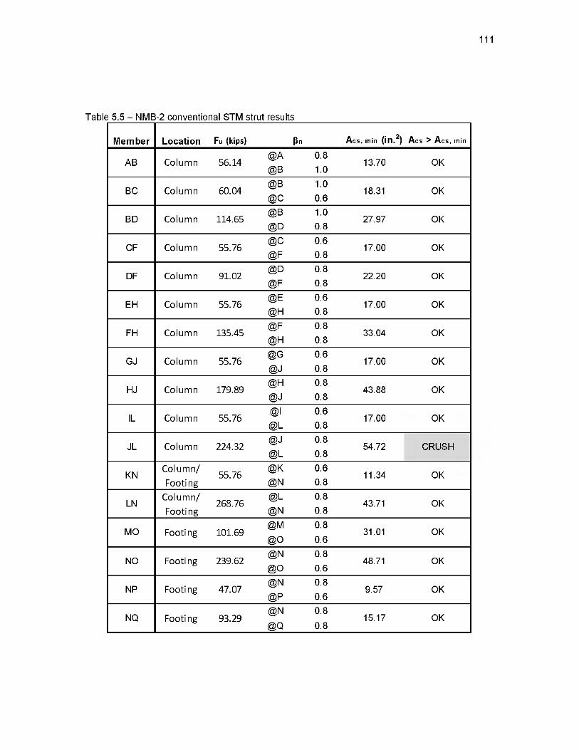
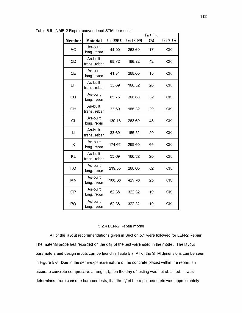
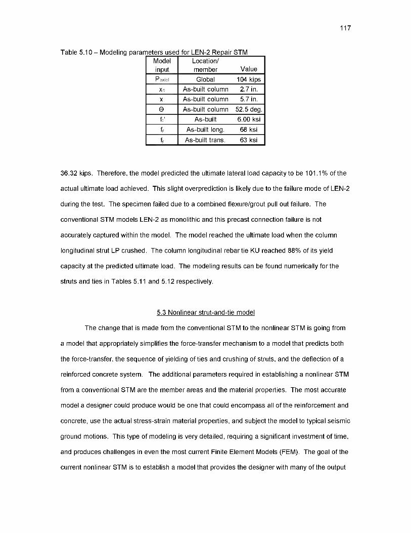
5.3 Nonlinear strut-and-tie model.......................................................................................1175.3.1 Member areas.............................................................................................. 1215.3.2 Member material properties........................................................................ 1245.3.3 Determination of ultimate displacement.....................................................1305.3.4 NMB-2 Repair model....................................................................................1325.3.5 NMB-2 model.................................................................................................1375.3.6 LEN-2 Repair model.....................................................................................1425.3.7 LEN-2 model..................................................................................................147

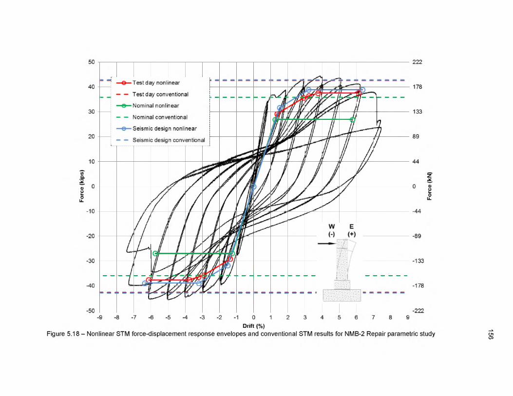
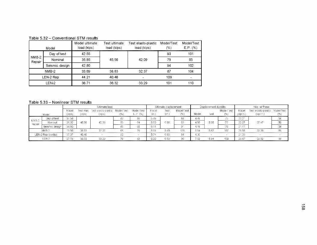
5.4 Parametric study of strut-and-tie model material design values...............................1525.4.1 Conventional strut-and-tie model................................................................1535.4.2 Nonlinear strut-and-tie model .....................................................................154

5.5 Comparison of strut-and-tie model results to test data ..............................................1575.5.1 System results ............................................................................................. 1575.5.2 CFRP results.................................................................................................1625.5.3 Headed rebar results....................................................................................163

6. CONCLUSIONS............................................................................................................................ 165

vii

6.1 Repair design recommendations..................................................................................1676.2 Recommendations for future research........................................................................ 168

REFERENCES.................................................................................................................................. 170

viii

ACKNOWLEDGEMENTS

I would like to thank the members of my supervisory committee, Dr. Chris Pantelides, Dr.

Lawrence D. Reaveley, and Dr. Evert Lawton, for their support in this research. Special thanks to

my advisor and chairman of the committee, Dr. Chris Pantelides, for the guidance, mentorship,

and countless hours that he has dedicated to this project. I would like to acknowledge and thank

the other graduate students working on this project, M.J. Ameli and Joel Parks. Thanks to Mark

Bryant, the University of Utah Structures lab manager, for all of the assistance in the laboratory.

Additionally I would like to thank the Mountain Plains Consortium, the Utah Department of

Transportation, Texas Department of Transportation, New York Department of Transportation,

NMB Splice Sleeve, Headed Reinforcement Corp., Sika Corporation, and Hanson Structural

Precast for their contributions to this research.

CHAPTER 1

INTRODUCTION

Bridge design philosophy is shifting beyond simply providing structures that will not

collapse during a large earthquake and moving towards performance based design in which

acceptable damage states after an earthquake are being prescribed. An example of this shift is

illustrated by CALTRANS limiting the allowable displacement ductility to a value between four and

five (1) for bridge columns. Limiting the amount of displacement ductility controls the amount of

permanent damage the bridge experiences from the design earthquake and allows for potentially

repairing the damaged structure. It is not possible to design bridges that will remain undamaged

during an earthquake due to the high cost of materials, uncertainty in loading, and design time

necessary to build such a structure. Therefore, repair procedures that can rehabilitate a bridge

after an earthquake are necessary to avoid the cost, construction time, and interruption to

emergency services and the general public that bridge replacement causes.

Accelerated Bridge Construction (ABC) is gaining popularity and is used nationwide due

to decreased user interruption and increased safety of the construction personnel. Grouted

Splice Sleeves (GSS) are gaining attention as a method for connecting precast concrete bridge

elements using ABC standards. The use of GSS connections for bridge elements in areas of

high seismicity is currently being studied (2-4). Recent projects, including the construction of the

FrontRunner light rail train bridges in Salt Lake City, show the promise for GSS becoming a

popular precast concrete connection option in areas of high seismicity. The expected increase in

use of GSS connections poses the need for a postearthquake repair technique, which is the focus

of this study.

2

Since current code directed capacity-based bridge design directs the damage of bridge

assemblies into the columns, thus protecting the footings and pier caps, the repair has been

developed for column plastic hinges. The repair method developed in this project uses Carbon

Fiber-Reinforced Polymer (CFRP) shells, headed mild steel rebar, and nonshrink or expansive

concrete to strengthen the column plastic hinge region, relocating subsequent damage above the

repaired section. This plastic hinge relocation is achieved by increasing the column cross­

section. On the half-scale specimens tested in the current study the column was increased from

a 21 in. octagonal section to a 30 in. diameter circular section over a column height of 18 in. The

repair can be implemented rapidly and uses standard construction techniques and a small

amount of readily available materials. The purpose of the repair is to restore the diminished load

and displacement capacities of an earthquake damaged column, alleviating the need for bridge

replacement.

Two precast concrete bridge column-to-footing assemblies connected using GSS have

been tested to failure under quasi-static cyclic lateral loads and a constant axial load, simulating

earthquake loading. These assemblies were then repaired using the repair method developed in

this study and retested cyclically. The results of the tests for the repaired specimens were then

evaluated and compared to the performance of their undamaged precast counterparts.

To aid in the design of both the undamaged and repaired specimens, conventional and

nonlinear Strut-and-Tie Models (STM) were developed using generic modeling parameters. The

conventional model uses the STM procedures outlined in ACI 318 (5) to predict the ultimate load

capacity of the assembly being modeled. The nonlinear STM expands upon the conventional

STM by using nonlinear material properties, which incorporate allowable strengths reflecting the

effects of cyclic degradation, to predict the nonlinear force-displacement response envelope of an

assembly that is subjected to lateral load reversals.

1.1 Literature review

The literature review for this research is separated into three parts: the cyclic performance

of GSS connections, bridge column retrofit and repair, and STM analytical findings.

3

1.1.1 Cyclic performance of GSS connections

GSS have been used for bridge column connections in nonseismic regions in the past.

Recently, research programs at the University of Utah (2), University of Nevada at Reno (3), and

University of Bergamo (4) have begun to investigate the applicability of GSS connections is

seismic regions. The findings from these research programs are showing acceptable levels of

cyclic performance for the GSS connections. However, the precast specimens do not match the

performance of their monolithic counterparts in terms of displacement ductility and energy

dissipation. The specimens that are referred to as the “as-built” specimens in this study are the

precast concrete column-to-footing GSS specimens being studied at the University of Utah (2).

1.1.2 Bridge column retrofit and repair

Extensive research has been conducted on retrofit and repair techniques for bridge

columns utilizing CFRP composites (6, 7), steel (8), and concrete jacketing (9). The objective of

these studies was to increase the flexural performance of the column plastic hinge region through

jacketing. Recently, a precast concrete specimen connected using GSS was repaired after

being tested cyclically (4). The repair consisted of a grout jacket made from high-strength

shrinkage-compensating grout. The exact details of the retrofit are not known, but the results

were unsatisfactory in terms of displacement ductility and energy dissipation capacity.

Little research has been conducted that investigates plastic hinge relocation as a method

to control the location of damage or to restore diminished load and displacement capacities of

earthquake-damaged bridge columns. Hose et al. (10) studied the effectiveness of strengthening

likely plastic hinge regions to force damage away from joint regions. The plastic hinge regions

were successfully relocated by increasing the longitudinal and transverse reinforcement ratios in

the traditional plastic hinge regions. Lehman et al. studied multiple concrete jacketing

techniques, including techniques to relocate the original plastic hinge, on columns of varying

damage states (9). One repair, performed on a column with fractured longitudinal rebar,

increased the original column cross-section from a 24 in. to 30 in. diameter cross-section over a

column length of 22 in. The increased cross-section was reinforced with double headed rebar in

4

the longitudinal direction and a spiral at a 1.5 in. pitch in the transverse direction. The intent of the

repair was to relocate the plastic hinge region to the top of the repaired section. The repair was

successful but did not restore the diminished displacement capacity of the specimen. Recently,

Rutledge et al. have used CFRP oriented in the longitudinal and transverse directions to perform

plastic hinge relocation on earthquake-damaged monolithic column-to-footing specimens (11).

The damage state of the specimens prior to repair was severe, including longitudinal rebar that

had buckled or fractured. Three tests were performed on the repaired specimens; plastic hinge

relocation was achieved for specimens which had buckled rebar. However, the repair proved

incapable of restoring the diminished load and displacement capacities if the longitudinal rebar

had fractured prior to the repair.

1.1.3 Strut-and-tie models

Strut-and-Tie Modeling (STM) is an accepted and well documented approach for analysis

of reinforced concrete elements with disturbed-regions (D-regions). National bridge and building

codes (5, 12) have adopted STMs as an applicable analysis procedure for D-regions. The STM

design method prescribed in ACI 318 (5) is referred to as the conventional STM method within

this study. The use of conventional STMs to design members that utilize CFRP has recently

been investigated for shear transfer across precast concrete joints (13) and deep beams

strengthened with CFRP (14). Additionally, the development of headed rebar has been modeled

for exterior beam-column joints using a conventional STM (15).

Recently, To et al. (16-18) have added modeling parameters that expanded upon the

conventional STM to predict the force-displacement response envelopes of a specimen, referred

to as nonlinear STMs. The modeling parameters that are needed to shift from the conventional

STM to the nonlinear STM are the material force-displacement properties and the STM member

areas. To et al. (16) describe methods to determine both of these parameters, including the

effect that cyclic degradation plays on the material properties. The nonlinear STM has been

further expanded to predict the hysteretic response and failure mode of structural systems using

nonlinear STMs (19, 20).

5

1.2 Overview of tests

The focus of this study is the development of a repair procedure for earthquake-damaged

modern bridge column-to-footing specimens connected using GSS couplers. In order to design

and test the repaired specimen, a damaged specimen must first be created, and the damage

state must be assessed. Two tests were performed on undamaged precast column-to-footing

specimens connected using GSS, referred to as the as-built specimens. After testing and

assessing the performance of the as-built specimens, a repair procedure was developed and

implemented for both damaged specimens. The repaired assemblies were then retested

following the same procedures as the as-built specimens. After the completion of the repair for

the as-built specimens, the assemblies are referred to as the repaired specimens.

The column-to-footing specimens were tested in single curvature, replicating an idealized

subsection of a multicolumn bridge subassembly that is subjected to double curvature. The

bridge subsection that is being tested is the column-to-footing portion of the bridge subassembly

from the point of inflection down, as shown in Figure 1.1. The specimens were designed to be

half-scale of typical bridge elements in Utah. The soil-structure interaction at the footing-soil

interface was neglected and the footing was secured to a rigid strong floor. All of the as-built and

repaired specimens were tested laterally with a constant axial load of 6% of the column’s 28-day

concrete strength axial load capacity, representing typical axial loading of bridge structures. The

lateral load was applied following a displacement controlled quasi-static cyclic loading protocol,

which remained the same for all tests.

1.2.1 As-built tests

Two precast column-to-footing as-built specimens were constructed, instrumented, and

tested in the University of Utah Structures Laboratory. The columns were 8.5 ft. tall and had a 21

in. wide octagonal cross-section. The footings were 6 ft. long, 3 ft. wide, and 2 ft. deep. Both as-

built specimens were precast as two separate pieces, a column and a footing, and later

connected using GSS couplers. The first as-built specimen to be tested, NMB-2, was built with

the GSS located in the footing, and the second as-built specimen to be tested, NMB-3, was built

6

Figure 1.1 - Test explanation: (a) Idealized bridge subassembly subjected double curvature, (b) Tested subsection of bridge subassembly

7

with the GSS located in the column. The footing bars in NMB-3, which were left extending out of

the concrete to grout with the GSS, were debonded for 8 in. below the footing concrete surface.

The column and footing of both specimens were designed adhering to current seismic bridge

design standards (21).

1.2.2 Repaired tests

After testing the as-built specimens, they were evaluated in terms of their damage state,

and a repair procedure was developed to restore their diminished performance. Both as-built

specimens experienced flexural failure, with plastic hinging occurring in the column and footing at

the column-footing interface. Longitudinal rebar fracture occurred in the plastic hinge region of

both as-built specimens. The repair designed for NMB-2 and NMB-3 was identical due to their

similarities in reinforcement, geometry, and damage states prior to repair. The plastic hinge

region from the as-built test was repaired by increasing the column cross-section from a 21-in.

octagonal section to a 30-in. diameter circular section over an 18 in. length. The 30-in. diameter

circular cross-section was constructed using prefabricated CFRP shells. Headed mild steel bars

were epoxy-anchored into the footing within the CFRP shell, and nonshrink or expansive concrete

was used to fill the void between the original column and CFRP shell. The repair was designed

to relocate the plastic hinge to the column section adjacent to the repaired section, which

remained relatively undamaged during the as-built test.

After the repair procedure was complete for NMB-2 and NMB-3, they were renamed

NMB-2 Repair and NMB-3 Repair, respectively. Both NMB-2 Repair and NMB-3 Repair were

tested with the same axial load and lateral loading protocol as their as-built counterpart. The

load, displacement, and instrumentation results were then analyzed and compared with the as-

built results to determine the effectiveness of the repair.

1.3 Overview of strut-and-tie modeling

Strut-and-Tie Models (STM) were developed for the as-built and repaired specimens.

STM are commonly used models to design reinforce concrete elements within D-regions of

8

structures. The purpose of the models was to develop STM procedures that could be used by

designers with varying needs. To accomplish this, generic modeling parameters were developed

that could be implemented on different reinforcement layouts and element geometries. Two

types of STM were developed for the as-built and repaired specimens: a conventional STM and a

nonlinear STM. The specimens modeled were NMB-2, NMB-2 Repair, LEN-2, and LEN-2 Repair.

LEN-2 is a precast column-to-pier cap specimen connected using a different type of GSS than

NMB-2. LEN-2 Repair is the repair of LEN-2 after the as-built test. LEN-2 Repair was repaired

following the same procedure as NMB-2 Repair and NMB-3 Repair.

1.3.1 Conventional STM

The conventional STM method was developed following the modeling procedures outlined

in ACI 318 (5). The model provides the designer with an estimate of the ultimate lateral load

carrying capacity of the assembly. However, the STM procedure within ACI 318 is not intended

to be used to analyze elements within a lateral-force resisting system. In addition, the parameters

needed to predict the displacement response are generally neglected, leaving only a prediction of

the force response.

1.3.2 Nonlinear STM

The nonlinear STM has been developed to provide the designer with an estimate of the

force-displacement response envelope of the assembly being modeled. From the nonlinear STM

response envelope the ultimate load and displacement can be predicted as well as the yield

displacement, displacement ductility, and stiffness. Modeling recommendations given by To et al.

(15-17) have been adopted in this study.

To obtain displacements from an STM model, the member areas and material properties

must be known. To accurately predict the response of a specimen which is undergoing cyclic

load reversals, material properties that account for the cyclic degradation of the materials must be

used. Also, nonlinear steel reinforcement and CFRP confined concrete models have been used

9

to accurately obtain displacements from the model. Member areas that represent the state of

stress at first yield have been adopted.

CHAPTER 2

EXPERIMENTAL SETUP AND RESULTS FOR

AS-BUILT SPECIMENS

The specimens referred to as “as-built” are the precast concrete column-to-footing

specimens prior to the repair. After cyclically testing the as-built specimens, they were repaired

and retested. The details of two as-built specimens will be discussed in this section, NMB-2 and

NMB-3 (2).

2.1 As-built specimen details

Both NMB-2 and NMB-3 are precast reinforced concrete specimens. The specimens were

precast as two separate elements, a column and a footing, and later attached using Grouted

Splice Sleeve (GSS) connections. The GSS connections used were NMB splice sleeves, size

8U-X, as shown in Figure 2.1. NMB-2 had the GSS connectors precast into the footing, and

NMB-3 had the GSS connectors precast into the column, as seen in Figure 2.2. The GSS

connectors are precast into an element with rebar from the connecting element extending into the

sleeve. Special care is taken to ensure that the sleeve remains void of concrete during casting.

Upon assembly, rebar protruding from the concrete of the element without the GSS connectors

are inserted into the sleeves. The bars that extend from the element cast without the GSS are

referred to as field dowels. Both the field dowels and the bars cast into the GSS are grouted with

a high strength nonshrink grout to complete the connection. This type of GSS connection uses

grout to secure the rebar at both ends of the connection.

The reinforcing details of both the column and footing adhere to current bridge design

specifications (12, 21). The longitudinal and transverse reinforcement ratios in the column are

11

12

1.3% and 1.9%, respectively, conforming to both AASHTO and CALTRANS requirements (1).

The column cross-section is nonprismatic with a 21-in. square top section extending 18 in. from

the top of the column, changing to a 21-in. octagonal section for the rest of the column length.

The square top was designed to easily connect with the lateral load application system. The

octagonal column cross-section was used over the length being tested to match the current

bridge geometry used by the Utah Department of Transportation. The octagonal cross-section is

7 ft. long and includes the probable plastic hinge region at the column-footing interface. The

footing is 6 ft. long in the direction of the lateral load application, 3 ft. wide and 2 ft. deep. The

sizes of the elements were designed to be approximately half-scale of typical bridge dimensions.

The reinforcement details for NMB-2 are shown in Figure 2.3. The column reinforcement

consists of six no.8 longitudinal steel bars and a no.4 spiral at a pitch of 2.5 in. The NMB-2

footing reinforcement consists of 18 no.8 longitudinal steel bars, a no.4 joint spiral, and two

overlapping no.4 stirrups spaced at 2.5 in. on center.

The reinforcement details for NMB-3 are shown in Figure 2.4. The column reinforcement

consists of six no.8 longitudinal bars and two no.4 spirals at a pitch of 2.5 in. The additional spiral

used in the column of NMB-3 is provided for shear reinforcement around the GSS connections.

Two different spirals were required since the perimeter around the GSS is larger than the

perimeter of the longitudinal reinforcement. The NMB-3 footing reinforcement consists of 18 no.8

longitudinal bars and two overlapping no.4 closed stirrups at 2.5 in. on center. The six no.8 field

dowel bars were debonded in the footing just below the concrete surface for a length of 8 in.,

corresponding to 8 bar diameters. The debonding was implemented to postpone the longitudinal

rebar from fracturing by increasing the strain capacity of the bars by distributing the plasticity over

a greater length. Debonding was achieved by wrapping the bars with three layers of adhesive

tape over the length in which debonding was desired.

Both the NMB-2 and NMB-3 rebar cages prior to concrete casting are shown in Figure 2.5.

The all thread rods that are tack welded onto the longitudinal rebar of the column are used to

connect instrumentation.

■21 IN-

SECTION B-B

Figure 2.3 - NMB-2 reinforcement details

CO

ure 2.4 - NMB-3 reinforcement details

#4 SPIRAL JOINT REINFORCEMENT

#4 CROSS-TIE

#4 JOINT U STIRRUPS

SECTION C-C

3 FT.

-6 F T -

SECTION D-D

15

’ ■(C) (d)

Figure 2.5 - Rebar cages: (a) NMB-2 column, (b) NMB-2 footing, (c) NMB-3 column, (d) NMB-3 footing

2.2 Test assembly

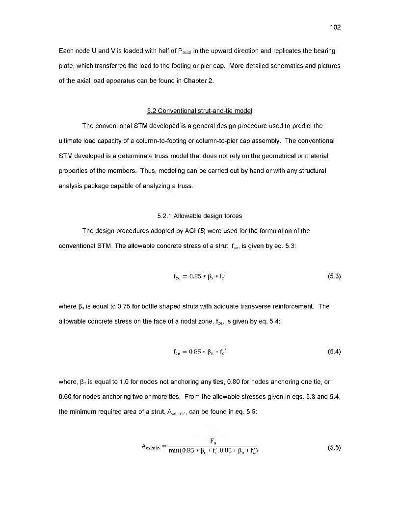
All of the as-built and repair tests were conducted in the University of Utah Structures

Laboratory. The primary test components are the loading frame, the lateral load system and the

axial load assembly which remained the same for all of the as-built and repair tests. The lateral

load system relies on the loading frame to provide the necessary reaction to displace the

specimen, while the axial load assembly is self-contained. These three experimental components

create the boundary conditions for the tests and will be discussed in this section.

16

2.2.1 Loading frame details

The loading frame, also referred to as the structures bay, consists of steel W sections

anchored into a strong floor, as shown in Figure 2.6. The lateral load system relies on the

structures bay to provide an equivalent lateral reaction to balance the load needed to displace the

test specimen. Since the loading protocol is displacement controlled, the deflection of the

structures bay when providing the reaction to the lateral load system is critical. The structures

bay was modified to minimize lateral deflection by increasing the stiffness of the girder used to

attach the lateral actuator. The increase in stiffness was achieved by welding web stiffeners onto

the girder on either side of the actuator, welding a steel W section on its side to the back of the

girder, and by welding steel HSS tubing from the additional W section to another member of the

structures bay, shown in Figure 2.6.

Another function of the loading frame is to provide the necessary reactions for the test

specimens. These reactions were achieved by anchoring the specimens to the strong floor with

high strength, 150 ksi, threaded steel rods. Each end of the footing was connected with eight

high strength rods, four of which ran through PVC pipes embedded into the concrete and four of

which were outside the concrete. These rods were then tensioned prior to testing to prevent the

specimens from rocking or slipping on the strong floor.

2.2.2 Lateral load application system

The lateral load is applied to the test specimens 96 in. above the top of the footing. This

point represents the theoretical inflection point of a bridge column that is subjected to double

curvature. Double curvature is present in bridges between the pier cap and footing when

subjected to earthquake loading. The lateral load system consists of an actuator, load cell, and

spherical bearing connection, as shown in Figure 2.7. The actuator has a capacity of 120 kips

and is servo-controlled. A pin connection secures the actuator to the stiffened loading frame

girder. The actuator piston is threaded into a 200 kip load cell. This load cell then threads into a

machined splice that attaches the test specimen to the load cell through a spherical bearing.

17

Figure 2.6 - Loading frame: (a) Entire frame, (b) Web stiffeners added on either side of lateral actuator, (c) Stiffened girder

W E

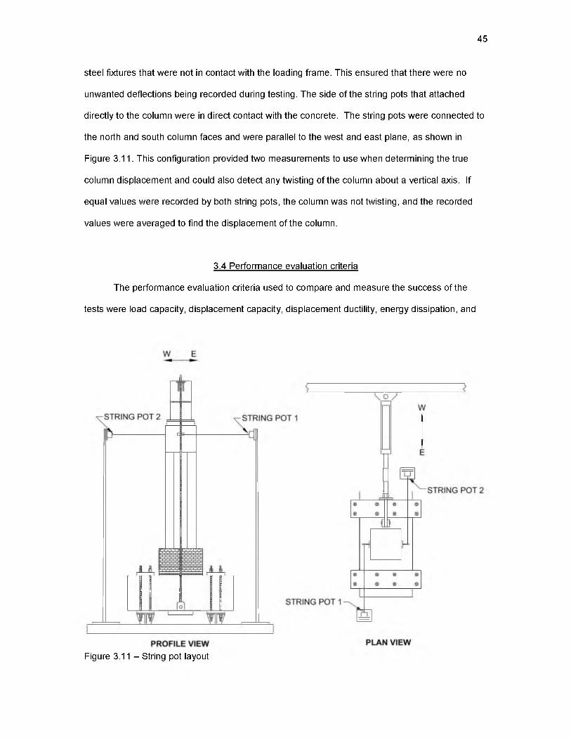
Figure 2.7 - Test assembly details

s

MODIFIED W 14 X 90

00

19

2.2.3 Axial load assembly

The axial load apparatus does not rely on the loading frame. The axial load is self­

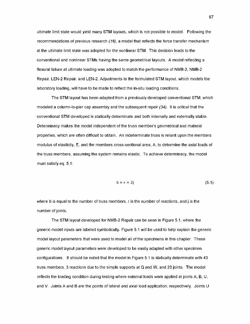
contained within the specimen, where the reactions are provided from the top of the column and

the bottom of the footing, shown in Figure 2.7. The 500 kip hydraulic axial actuator is located on

top of the column and rests on a spherical bearing plate, which allows biaxial rotation. At the

base of the footing there is a 10-in. wide by 3-in. thick plate that is pulled against the bottom of

the footing by the axial load rods, which are tensioned by the actuator. The axial load rods,

which connect the W-section on top of the axial actuator to the base plate, are pinned at the base

plate to allow rotation of the rods while the assembly is displaced. It should be noted that NMB-2

Repair had the axial load apparatus as detailed in Figure 2.7 while NMB-3 Repair had additional

pin connections where the high strength rods connect to the W-section. To achieve a constant

axial load, curvature within the high-strength rods should be avoided, and is the reason for the

additional pin connection.

2.3 Loading protocol

The applied loading during testing consisted of the axial and lateral loads. Both of these

loading components have unique loading protocols. The loading protocol described in this

section was used for all of the as-built and repair tests.

2.3.1 Axial load

The axial load applied during testing was designed to remain constant at 6% of the axial

load capacity of the column. Typically bridge structures are subjected to small amounts of axial

load in comparison to the column sizes that are provided; 6% of the gross column capacity is a

reasonable estimate of typical bridge axial loading. The axial load applied during testing, Paxiai,

was calculated from eq. 2.1:

Paxiai = 0.06 * Ag * fc' (2.1)

20

where Ag is the gross cross-sectional area of the octagonal column cross-section and fc’ is the 28-

day cylinder compressive strength of the concrete. From eq. 2.1 the target axial load was

determined, and the corresponding strain in the axial load rods needed to achieve Paxiai was

determined. There was slight deviation in the applied axial load and Paxial due to uneven straining

of the axial load rods and the incremental increase in strain from the actuator. During testing it

was observed that there was fluctuation in the axial load as the specimen was deflected in either

direction. This variation in axial load was captured by the strain gauges located on the axial load

rods. The variation in axial load was always an increase as the specimen was displaced. Since

there was no load cell monitoring the axial load, the exact variation in axial load is not known;

however, from the axial load rod strain gage data it appears that this variation is small.

2.3.2 Lateral load

All of the tests were conducted with a displacement controlled reversed quasi-static cyclic

lateral loading protocol. The applied lateral loading displacement history used was the same for

all tests so that the hysteretic behavior could be easily compared. The applied lateral

displacement history can is shown in Figure 2.8. The first peak displacement used corresponds

to half of the predicted yield displacement of the as-built specimens. Each subsequent peak

displacement is an integer multiplier of the predicted yield displacement. Each peak

displacement was carried out for two cycles where each cycle consisted of the peak displacement

in both the positive and negative direction. The positive displacement, a displacement to the

east, is applied before the negative displacement, a displacement to the west, during each cycle.

A 5-minute pause was programed into the loading protocol between each displacement step to

allow inspection of the test specimens. This applied lateral loading protocol follows the

recommendations of ACI Committee 374 (22).

2.4 As-built specimen test results

The as-built specimen tests were part of a separate research project, conducted at the

University of Utah, which is looking into the seismic performance and applicability of GSS

21

10

8

6

4

2

£ 0 k_Q-2

-4

-6

-8

-100 2 4 6 8 10 12 14 16 18 20

CycleFigure 2.8 - Applied lateral displacement history

connections for bridges in seismic regions (2). However, to understand the results of the repaired

specimens it is crucial to know both the performance and the final damage state of the as-built

specimens.

2.4.1 NMB-2 results

On March 8th, 2013 NMB-2 was tested and brought to failure in the University of Utah

Structures Laboratory. NMB-2 was a precast concrete column-to-footing assembly that had GSS

located in the footing. Details pertaining to NMB-2 can be found in Section 2.1. The hysteretic

response of the specimen is shown in Figure 2.9, and the damage state during the final

displacement step, of 7 in., and after testing is shown in Figure 2.10. It can be seen from the

hysteresis that the ultimate load achieved during testing was 38.8 kips. The failure mode of the

specimen was crushing of the column concrete followed by longitudinal rebar facture. The east

extreme longitudinal bar fractured during the first cycle of the 7-in. displacement step,

approximately 3 in. above the top of the footing. The lateral load capacity in the west direction of

testing was severely diminished when the east longitudinal rebar fractured. The lateral load

22

Figure 2.9 - NMB-2 hysteresis curve

capacity in the west direction, after the longitudinal rebar fractured, dropped to 65% of the

ultimate lateral load capacity in that direction. The 7-in. displacement step was never completed

due to a weld failing that secured the south axial load rod to the base plate of the axial load

assembly.

A plastic hinge is evident at the column-footing interface of NMB-2, with spalling extending

up the column 8 in.—12 in. on the west and east extreme column faces. Structural cracking of the

column occurred at three levels located approximately 6 in., 10 in., and 14 in. above the footing.

The maximum crack width at the 6 in., 10 in., and 14 in. levels during the pause between cycles

was 0.050 in., 0.025 in., and 0.030 in., respectively. Cracking extended up the column higher

than 14 in. but remained hairline in width throughout testing.

23

(c) (d)

Figure 2.10 - NMB-2 damage state at final displacement step and after testing: (a) Ultimate displacement of 7 in., (b) Final column and footing cracking after testing, (c) Plastic hinge region, (d) Fractured east longitudinal rebar
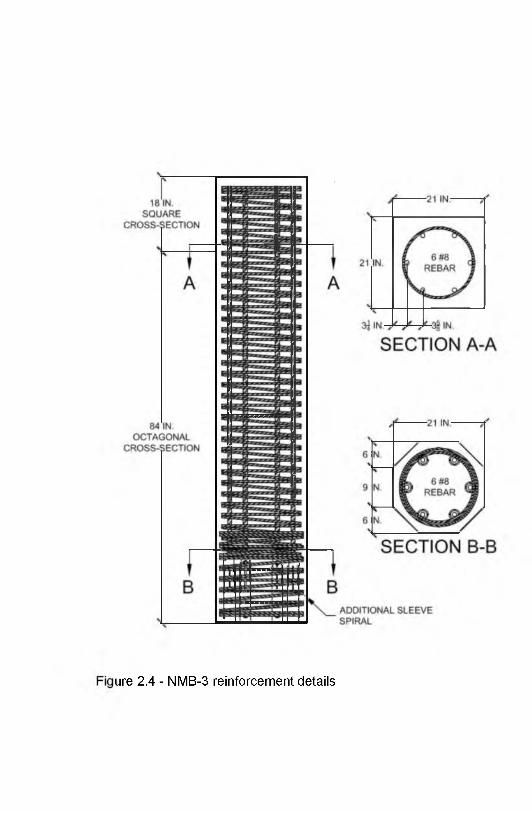
2.4.2 NMB-3 results

On August 29th, 2013, NMB-3 was tested and brought to failure in the University of Utah

Structures Laboratory. NMB-3 had GSS located in the column and had a debonded rebar in the

footing. Details pertaining to NMB-3 can be found in Section 2.1. The hysteretic response of the

specimen is shown in Figure 2.11. It can be seen from the hysteresis that the ultimate load

achieved during testing was 42.0 kips. After the ultimate lateral load was achieved, during the 5­

in. displacement step, the east extreme longitudinal rebar fractured during the 8-in. displacement

24

Figure 2.11 - NMB-3 hysteresis curve

step. The east extreme longitudinal rebar ruptured at the column-footing interface during the first

cycle of the 8-in. displacement step. The lateral load capacity of the specimen when tested to the

west was severely diminished after the longitudinal rebar fractured. The lateral load capacity in

the west direction after the fracture dropped to 63% of the ultimate lateral load capacity. The

damage state of NMB-3 during the final displacement step and after testing can be seen in Figure

2.12. A plastic hinge was evident at the column-footing interface with spalling extending up the

column 12-16 in. on the west and east extreme column faces. However, there was noticeably

less damage at the column-to-footing interface than during the NMB-2 test, indicating that the

plasticity was forced into the footing due to the debonded bars. Structural cracking of the column

occurred at two levels located approximately 14 in. and 23 in. above the footing. The maximum

crack widths, measured during the pause between displacement steps, were 0.020 in. and 0.007

in. for the 14 in. and 23 in. crack levels, respectively.

25

Figure 2.12 - NMB-3 damage state at final displacement step and after testing: (a) Ultimate displacement of 7 in., (b) Plastic hinge region after testing, (c) Gapping between the column and footing, characteristic of the rocking behavior, (d) Seven levels of concrete cracking

26

During testing, the specimen demonstrated rocking behavior in the joint region. The

rocking is thought to be due to the GSS being located in the plastic hinge region of the column,

which increased the stiffness of the region and forced the plasticity of the specimen into the

footing where the debonded rebar were located. This characteristic led to smaller crack widths in

the plastic hinge region. More layers of cracking were observed in NMB-3 than in NMB-2, but

only two of the seven layers were larger that hairline.

CHAPTER 3

DESIGN, IMPLEMENTATION, AND EVALUATION METHODS

FOR REPAIRED SPECIMENS

After testing NMB-2 and NMB-3, a repair strategy was developed to restore the diminished

load capacity of the specimens. The same repair procedure was employed on both NMB-2 and

NMB-3. Once repaired, NMB-2 and NMB-3 were renamed NMB-2 Repair and NMB-3 Repair

respectively. Both NMB-2 and NMB-3 experienced longitudinal rebar fracture of the east extreme

bar. The damage state of both NMB-2 and NMB-3 at the time of repair is described in Chapter 2.

The process of repair consists of two parts, the design and the implementation. Both processes

are critical to the success of the repair. This chapter outlines the design and construction of the

repair as well as the instrumentation and performance evaluation criteria used to evaluate the

repaired specimens.

3.1 Repair design

The objective of the repair is to reestablish the load and displacement capacity of a

column-to-footing assembly by relocating the plastic hinge region from the column-footing

interface to the column-repair interface. To achieve a successful repair, the original plastic hinge

region must be strengthened sufficiently to withstand additional shear and moment demand that

the plastic hinge relocation will produce. The bending moment that causes plastic hinge

formation, MPH, must be reached at the desired plastic hinge location, and a bending moment

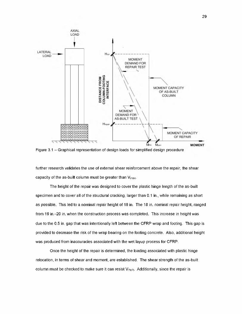
referred to as, Mjoint, must be resisted at the column-footing interface. MPH can be determined

from a sectional analysis or from test results. From eq. 3.1 it can be seen that MJoint is

28

proportional to the height of the repair, Hrepair, and the height of the column from the point of

inflection to the column-footing interface, Hcoi.

MphM

Therefore, using the minimum possible repair height is advantageous for limiting the

moment demand at the column-footing interface and for decreasing the rotational demand on the

column for a given displacement. On the other hand, the height of the repair must be long enough

to relocate the new plastic hinge to a minimally damaged cross-section. The ultimate moment

demand and required moment capacity for an as-built and repair specimen is shown in Figure

3.1.

From Mjoint, the shear that must be resisted in order to achieve plastic hinge relocation,

VPHR, can be found from eq. 3.2:

Vp„R = ^ (3.2)col

Similar to moment demand, the shear demand is directly related to the height of the

repair. This relationship can be seen by substituting eq. 3.2 into eq. 3.1, yielding eq. 3.3:

MpHVp„ R = H----T u ------- (33)

n col n repair

From both eq. 3.1 and 3.3 it can be seen that the repair height should be kept to a

minimum to reduce the moment demand on the repair and the shear demand on the column.

The shear capacity of the repaired cross-section will be much higher than the shear capacity of

the as-built column. Since the shear demand is constant along the height of the column, it is

likely that the shear capacity will be controlled by the as-built column shear capacity. Unless

29

M ph Mjoim

Figure 3.1 - Graphical representation of design loads for simplified design procedure

further research validates the use of external shear reinforcement above the repair, the shear

capacity of the as-built column must be greater than VPHR.

The height of the repair was designed to cover the plastic hinge length of the as-built

specimen and to cover all of the structural cracking, larger than 0.1 in., while remaining as short

as possible. This led to a nominal repair height of 18 in. The 18 in. nominal repair height, ranged

from 19 in.-20 in. when the construction process was completed. This increase in height was

due to the 0.5 in. gap that was intentionally left between the CFRP wrap and footing. This gap is

provided to decrease the risk of the wrap bearing on the footing concrete. Also, additional height

was produced from inaccuracies associated with the wet layup process for CFRP.

Once the height of the repair is determined, the loading associated with plastic hinge

relocation, in terms of shear and moment, are established. The shear strength of the as-built

column must be checked to make sure it can resist VPHR. Additionally, since the repair is

30

developed for specimens with fractured or highly damaged longitudinal rebar, the tension transfer

between the column and footing must be reestablished through the repair cross-section.

To achieve these design criteria, a repair was developed that increased the original

plastic hinge region from a 21-in. octagonal cross-section to an additionally reinforced 30-in.

diameter circular cross-section. Additional flexural reinforcement was provided in the form of

headed rebar. The headed bars were designed to increase the flexural strength of the repair and

reestablish the tension transfer between the column and footing. Additional shear reinforcement

was provided in the form of a unidirectional CFRP wrap. The CFRP wrap was designed to

provide shear strength and confinement to the repaired cross-section. The confinement that the

CFRP provides increases the capacity of the repair significantly by increasing the compressive

strength and strain capacity of the concrete within the repair.

The repair details are shown in Figure 3.2. There are three components for the repair

that must be designed: the headed rebar, the CFRP wrap, and the nonshrink/expansive concrete.

As usual with design, the different repair components are reliant upon one another, making the

design process iterative.

3.1.1 Headed rebar design

The headed steel bars are designed to increase the moment capacity of the repaired

cross-section to a value larger than Mjoint. The contribution of the as-built longitudinal rebar can

be conservatively ignored when determining the repaired cross-section moment capacity. This

assumption should be made when longitudinal bars have fractured in the as-built column prior to

repair. The moment capacity provided by the headed rebar is controlled by the area of steel that

is provided and the moment arm of the steel.

Placement of the headed rebar fixes the moment arm of each rebar and should be

determined from several design criteria. First, a clear spacing of 2 in. between the as-built

column and the center of the headed rebar should be maintained to allow space for drilling into

the footing. Space should also be provided between the headed rebar and the CFRP wrap to

31

S E C T I O N A - A

Figure 3.2 - Repair design details

allow proper bonding of the CFRP to the concrete and development of the headed rebar. Caution

should be taken when the clear spacing between headed rebar is small due to the group effects

that this creates. The headed rebar placement must minimize conflict with the longitudinal

reinforcement in the footing, which can be achieved by using a metal rebar detector to find the

longitudinal bars in the footing. Additionally, the smallest diameter possible for the CFRP wrap

should be selected to facilitate an economical design and to minimize interference with

surrounding objects when the repair is installed in the field. From these design criteria the

placement of the headed rebar and the diameter of the CFRP jacket can be designed iteratively.

In practice, the headed rebar should be distributed around the repair evenly since the direction of

lateral loading is not known.

With an estimate of the number of headed bars and placement, the minimum amount of

the headed bar area can be determined from eq. 3.4:

32

M n = A s * fy * ( d -0.8! > Mjoint

(3.4)

where Mn is the nominal flexural capacity of the repaired section, neglecting compression steel

and assuming zero axial load. Since the repair is built with the dead load applied to the bridge

and the axial load transfer between the as-built column and the repair is not known, neglecting

the axial load contribution to the moment strength of the repaired cross-section is appropriate: As

is equal to the cross-sectional area of the headed rebar in tension, fy is the nominal yield strength

of the headed rebar, d is the distance from the centroid of the headed rebar to the natural axis, fc’

is the nominal compressive strength of the repair concrete, and bw is the effective width of the

repair. An appropriate margin of safety should be maintained between the flexural capacity of the

section and the demand. These design equations lead to six no.8 grade 60 headed bars placed

as shown in Figure 3.2, with three headed bars on each side of the repair.

The length of epoxy anchorage into the footing and the amount of embedment into the

repair concrete must also be designed to provide proper development length. Since the repair

procedure is for bridge columns that are exposed to corrosive environments a clear cover of 3 in.

was provided between the top of the headed bars and the top of the repair concrete (5). This

cover requirement left a development length of 15 in. for the headed rebar in the repair concrete.

The required development length is determined from eq. 3.5 (5):

where ldt is the required development length for the headed rebar, is equal to 1.0 for nonepoxy

coated rebar, and db is the diameter of the headed rebar. For the no.8 rebar specified and a

conservative fc’ of 4000 psi, the required development length is 12.0 in., which is less than the 15

in. provided. Therefore the design is adequate.

33

Similar to the development length of the rebar in the repair concrete, the headed rebar

must develop in the epoxy anchorage within the footing. The required development length for the

epoxy anchorage, ld, is determined from eq. 3.6:

Ab * fvld = . b y (3.6)

du * Tt * T

where Ab is the cross-sectional area of one headed bar and t is equal to the specified bond

strength of the epoxy used. The epoxy used for the repair was Hilti HIT-RE 500-SD epoxy which

has a bond strength of 1400 psi (23). Using no.8 headed rebar, the required development length

is 12.2 in., which is less than the 19 in. provided. Therefore the design is sufficient.

3.1.2 Nonshrink/expansive concrete mix design

The concrete that filled the void between the as-built column and the CFRP wrap, referred

to as repair concrete, was designed differently for NMB-2 Repair and NMB-3 Repair. This was

the main design difference between the two repairs. The two different mix designs used for the

repair concrete in NMB-2 Repair and NMB-3 Repair are shown in Table 3.1. The repair concrete

that was used for NMB-2 Repair was designed as nonshrink concrete, whereas the repair

concrete for NMB-3 Repair was designed as expansive concrete. The time dependent expansion

results of the repair concrete for NMB-2 Repair and NMB-3 Repair can be found in Section 4.1.

The amount of expansion is controlled by the ratio of Komponent cement to Portland Concrete

Cement (PCC). Komponent is intended to produce nonshrink concrete when proportioned at

15% of the cementitious materials. The repair concrete in NMB-2 Repair and NMB-3 Repair had

Table 3.1 - Repair concrete mix designCementitious materials Water Aggregates

(lb/yd @ SSD)Additives (oz/yd)

Komponent(lb/yd) b

P

/ C

PercentKomponent

(%)Cold water

(lb/yd)

Water to cement ratio

(%)Point

3/4 in.Pointsand

Daravair (air entrainer)

G lenium 30-30 (super plastisizer)

NMB-2 Repair 92 599 13 280 41 1600 1060 6.5 49

NMB-3 Repair 262 370 41 280 44 1600 1060 6.5 49

34

Komponent percentages of 13% and 41% respectively. Previous research has shown that pre­

tensioning CFRP wraps significantly increases the load bearing capacity of the specimen (24,

25). However, caution should be taken to not overstrain the jacket when using expansive

cementitious materials to provide active pressure (26).

The purpose of the CFRP jacket is to provide confinement and shear strength to the

original plastic hinge region. Proper confinement increases both the strain capacity of the

confined concrete and its compressive strength. Research has shown that a minimum jacket

thickness and associated confinement are required to prevent strain softening of CFRP confined

concrete (27). Therefore, a jacket thickness was provided to ensure strain hardening of the

concrete within the jacket. The jacket was also designed to withstand all of the shear demand,

VPH, over the length of the repair. Although the as-built column has sufficient shear capacity to

resist VPH, the original plastic hinge region needs shear strengthening due to concrete crushing

and the spiral yielding during the initial test.

From previous research, the CFRP jacket thickness, j sh, required to ensure strain

hardening behavior of the confined concrete and provide proper confinement is determined by eq.

3.7 (27):

where fco is the unconfined concrete compressive strength; Ef is the CFRP modulus of elasticity;

Hc is the diameter of the CFRP jacket; ASH is a factor accounting for the aspect ratio of the CFRP

section and is equal to 12 for circular cross-sections; and Csh is the jacket confinement ratio

coefficient, which is equal to 1.0 for circular cross-sections.

The CFRP jacket thickness required for shear strengthening of circular column sections in

plastic hinge regions, j v, was determined from eq. 3.8 (6):

3.1.3 CFRP wrap design

(3.7)

35

XV j * 0.004 * Ef * Hc(3.8)

where VPH is the column shear demand; Ov is the shear capacity reduction factor, which was

taken as 0.85 (6); and Vc,,, Vs, and Vp are the shear capacity contribution of the concrete, shear

reinforcement, and axial load respectively. Due to the damage state of the original plastic hinge

region, Vc,, Vs, and Vp can all conservatively be taken as zero.

An additive approach to find the total jacket thickness needed for the repair, tj, totai, is

adopted by using eq. 3.9:

where tj, shell is an additional term for the CFRP shell required as formwork for the repair concrete.

For NMB-2 Repair and NMB-3 Repair, two layers of CFRP were provided to prevent strain

softening and provide confinement, one layer was provided for shear strength, and one layer was

provided as a shell for the repair concrete. The shell layer was used as a construction aid to

maintain the circular cross-sectional shape. Each CFRP layer has a nominal thickness of 0.04 in.

The first step in the repair procedure was creating the CFRP wrap. The CFRP wrap was

created from unidirectional SikaWrap Hex 103C fibers oriented in the hoop direction and Sikadur

Hex 300 Epoxy. The impregnation process was done by hand using a paint roller and abrasive

metal roller. Once saturated, the excess resin was scraped off of the CFRP using a rubber tool.

To create the prefabricated CFRP shells, used as stay-in-place formwork for the repair

concrete, a single layer of 18-in. wide CFRP was wrapped and cured around a 30-in. diameter

circular sonotube. After the CFRP shells had cured, they were cut into two half cylinders and

brought around the column. Although it would have been possible to bring the cylindrical shell

over the top of the column as one piece, the shell was cut in two to simulate the way this

tj,total ( tj,sh tj,v j,she 11 (3.9)

3.2 Repair procedure

36

procedure would be executed in the field. Once the shell was around the column, it was spliced

with a 12-in. long piece of CFRP for the height of the repaired column. The 12-in. splice length

was determined to provide proper development of the fibers on either side of the splice. Once the

splice was laid up, three additional 100-in. long layers of CFRP composite were wrapped around

the shell. The length of 100 in. was used to provide an overlap of over 5 in. for each layer.

Special care was taken to alternate the locations of the CFRP shell splice and for each additional

layer. The sonotube was left inside the CFRP shell to provide rigidity while the additional layers

of CFRP were applied; it was removed once all CFRP layers had cured. Figure 3.3 shows the

steps involved in preparing the CFRP shell.

While the CFRP shells were curing, the holes for the postinstalled headed bars were

core-drilled into the footing by Penhall Company. The holes were 1.25 in. in diameter, which

provided a radial clearance of 0.125 in. between the headed rebar and the hole. Upon

completion of drilling, the holes were prepared for the epoxy by cleaning and drying them.

Subsequently, Hility HIT-RE 500-SD epoxy was injected into the hole using a Hilti dispenser to

avoid the formation of air voids. The headed bars were inserted into the holes, and excess epoxy

was forced out of the top of the hole, indicating that a proper amount of epoxy was used. Figure

3.4 shows the steps involved in preparing the headed rebar.

Once the CFRP shell and epoxy for the headed rebar had fully cured, nonshrink/

expansive concrete was added to the space between the column and CFRP shell. The concrete

was vibrated to minimize the amount of air voids left within the repair concrete. A 0.5-in. tall

cylindrical piece of sonotube was secured under the CFRP shell to maintain the 0.5-in. gap

between the CFRP shell and the footing. The piece of sonotube also ensured that the CFRP

shell remained centered around the column. Wooden formwork was placed on the top of the

CFRP shell to enclose the concrete within the repair. Weights were then placed on top of the

formwork to keep the concrete from expanding vertically. The repair concrete was cured for at

least 28 days before testing. Figure 3.5 shows the steps involved in casting the concrete for the

repair process.

37

Figure 3.3 - CFRP preparation: (a) Saturation, (b) Making of prefabricated shells, (c) Prefabricated shells split into two, (d) Wet layup

38

Figure 3.4 - Headed rebar installation: (a) Core drilling, (b) Epoxy injection, (c) Inserting headed rebar, (d) After installation

39

Figure 3.5 - Repair concrete casting: (a) Before casting, (b) Vibrating concrete during casting, (c) Finishing concrete after casting, (d) Wooden formwork and weights in place after casting

40

3.3 Instrumentation

The instrumentation utilized during testing consisted of a load cell, strain gauges, Linear

Variable Differential Transformers (LVDTs), and string potentiometers (string pots). Although the

servo-controlled actuator recorded both load and position, only the load values were used in data

analysis. The displacement values obtained from the actuator included the movement within the

lateral load system and therefore have a small level of inaccuracy. Accurate displacement

readings were obtained from the string potentiometers.

3.3.1 Strain gauges

Strain gauges were used to measure the strain in the reinforcing steel, CFRP jacket, and

axial load rods during testing. All of the strain gauges that were not damaged in the as-built tests

were connected during the repaired assembly tests. Many of the strain gauges from the as-built

tests were damaged during testing and provided inaccurate readings during the repaired

assembly tests. During the repair process, strain gauges were placed on the headed rebar as

well as the CFRP jacket.

The strain gauges used during the NMB-2 Repair test were all MEM strain gauges that

record strains until the yield point. The bond between the strain gauge and steel is lost past yield

for the MEM strain gauges, and the readings are lost. During the NMB-3 Repair test both MEM

and TML strain gauges were used. The TML strain gauges are designed for high strain readings

and can read up to five times the yield strain of the steel bars.

Figure 3.6 shows the strain gauge sections that were present for the NMB-2 Repair and

NMB-3 Repair test. NMB-3 Repair had more strain gauges on both the wrap and headed rebar.

Due to geometrical conflicts the exact locations of strain gauges did not always fall onto the

designated section. This variation in placement is recorded in the naming scheme that has been

adopted, which gives the strain gauge number entered into the data acquisition system followed

by the height above the column footing interface in parentheses. The strain gauge schedules can

be seen in Figures 3.7 and 3.8 for NMB-2 Repair and NMB-3 Repair, respectively.

41

Figure 3.6 - Strain gauge sections for NMB-2 Repair and NMB-3 Repair

SG17( +14^ ) - i ^ ^ — SG29(+16j )-SG20(+14^)—^ SG30(+16^)-

SECTION 4-4 SECTION 5-5Figure 3.7 - Strain gauge locations for NMB-2 Repair

42

Figure 3.8 - Strain gauge locations for NMB-3 Repair

43

3.3.2 Linear variable differential transformers

Linear variable differential transformers (LVDTs) were mounted to NMB-2 Repair and

NMB-3 Repair to measure displacements at critical locations. The LVDTs were attached to the

west and east faces of the columns to obtain strain and curvature measurements. All-thread rods

were tack welded onto the as-built longitudinal rebar with couplers at either end to provide

attachment points for the LVDTs. An LVDT was placed on the west side of the footing to

measure the lateral displacement, or slip, of the footing during testing. Also, an LVDT was placed

under the footing east of the neutral axis to obtain deflection readings for the base of the footing.

Figures 3.9 and 3.10 show the LVDT layout during the NMB-2 Repair and NMB-3 Repair tests. It

should be noted that LVDTs no. 5 to no. 8 were not used during NMB-2 Repair test because the

hardware was not installed prior to casting.

The average curvature for an LVDT cell, O, was found following eq. 3.10:

<|> = — - (3.10)T W *h

where A and B are the LVDT readings on the tension and compression faces of a cell,

respectively. Extension is taken as a positive LVDT reading. W is the horizontal distance

between the LVDTs that recorded A and B, and h is the cell height. There were two LVDT cells

recording curvature during the NMB-2 Repair test and four LVDT cells recording curvature during

the NMB-3 Repair test. The two LVDTs that make up each cell are no. 1 and no. 2, no. 3 and no.

4, no. 5 and no. 6, and no. 7 and no. 8.

3.3.3 String potentiometers

String potentiometers (string pots) were used to measure the lateral displacement of the

column. The string pots were connected to the column was at the level of the actuator. The

distance between the string pot and the connection to the specimen was large in comparison to

the vertical deflections being induced on the specimens from the lateral displacement. Therefore,

the small angle approximation was made in all of the string pot readings, and the recorded

displacements were taken as the true lateral displacements. The string pots were mounted to

44

Figure 3.9 - Typical LVDT layout looking north with approximate dimessions

Figure 3.10 - Typical LVDT layout of east or west column face with approximate dimessions

45

steel fixtures that were not in contact with the loading frame. This ensured that there were no

unwanted deflections being recorded during testing. The side of the string pots that attached

directly to the column were in direct contact with the concrete. The string pots were connected to

the north and south column faces and were parallel to the west and east plane, as shown in

Figure 3.11. This configuration provided two measurements to use when determining the true

column displacement and could also detect any twisting of the column about a vertical axis. If

equal values were recorded by both string pots, the column was not twisting, and the recorded

values were averaged to find the displacement of the column.

3.4 Performance evaluation criteria

The performance evaluation criteria used to compare and measure the success of the

tests were load capacity, displacement capacity, displacement ductility, energy dissipation, and

Figure 3.11 - String pot layout

46

hysteretic stiffness. Different methods exist for obtaining these specific performance evaluation

criteria. To provide continuity between test results, standardized methods for obtaining the listed

performance evaluation criteria have been adopted for both the as-built and repaired specimens.

The exact procedure followed for each of the performance evaluation criteria will be described

within this section.

3.4.1 Lateral load capacity

The lateral load capacity of each specimen is defined as the maximum load recorded

during testing. Three values of lateral load capacity exist for a test: one for the east direction of

testing and one for the west direction of testing and an average value from both directions of

testing. The 120-kip load cell attached to the piston of the lateral actuator recorded the force

values induced on the specimen.

3.4.2 Displacement capacity

The displacement capacity of each specimen is defined as the average failure

displacement value reached in the east and west directions. The failure displacement is also

referred to as the ultimate displacement. Failure is defined as the point at which the specimen’s

lateral load carrying capacity has dropped to 80% of the maximum lateral load capacity in a given

direction. If failure occurs between two displacement steps, linear interpolation of the specimen’s

envelope curve is used to find the ultimate displacement.

The envelope curve is obtained from the specimen’s hysteretic curves. For each

displacement step, the points at which the specimen reaches the highest load, in both directions

of testing, are taken as points on the envelope curve. The envelope curve is then constructed by

connecting each deformation step point linearly. If failure did not occur for a specimen in a

certain direction of testing, the ultimate displacement is defined as the maximum displacement

achieved in that direction. String pots attached to the north and south faces of the column

recorded the displacement values for the specimens.

47

The displacement of a specimen is often shown as drift within this document. The drift is

often listed as a percent and is defined as the lateral deflection divided by the distance between

the top of the footing and the lateral load application. The distance between the top of the footing

and the point of lateral load application was used as the denominator when calculating drift for

both the as-built and repaired specimens.

3.4.3 Displacement ductility

The displacement ductility of a specimen, |aA, is defined by eq. 3.11:

where Au is equal to the ultimate displacement, as defined in section 3.4.2, and Ay is equal to the

yield displacement. Both Au and Ay are obtained from the specimen’s envelope curve.

Once the envelope curve is constructed, an idealized bilinear, elasto-plastic curve is fit to

the envelope to get the value of Ay. Ay is defined as the displacement at which the elasto-plastic

curve changes from elastic to plastic. The equal energy rule was used when constructing the

elasto-plastic curve, which states that the energy of the envelope and elasto-plastic curve must

be equal. Since the envelope and elasto-plastic curves are developed in force-displacement

space, the energy of each curve is simply the area underneath the curve. When following the

equal energy rule there are an infinite number of elasto-plastic curves that could be constructed

from an envelope. To ensure that there was only one possible bilinear curve that could be

developed for any given envelope, an additional modeling parameter was adopted to ensure

consistency between tests. The intersection of the elasto-plastic curve and the envelope curve

was set to 0.70 Ay (22). With this additional modeling parameter there is only one possible elasto-

plastic curve for any given envelope.

Once the elasto-plastic curve is developed, Au and Ay are defined, and the displacement

ductility can be calculated following eq. 3.12. For each test there are three different displacement

48

ductility values. There is displacement ductility for each direction of testing, and there is an

average displacement ductility value from both directions of testing. The average displacement

ductility is found from an average envelope curve. The average envelope curve is constructed by

averaging the absolute value of the envelope cures in both directions of testing for each

displacement step. From the average envelope curve, an elasto-plastic curve is developed

following the procedures described in this section, and the average envelope displacement

ductility can be calculated.

3.4.4 Energy dissipation

Energy dissipation capacity of a structural system is paramount to the seismic

performance of the system. The energy dissipation of a cycle is calculated from the area within

the hysteretic loop that is created during the cycle. For each displacement step, two cycles are

carried out, creating two hysteretic loops. The area of both loops was added to produce the

energy dissipation at the given displacement step. The results in this study are shown as the

total energy dissipated by the system at the conclusion of a certain displacement step, referred to

as the cumulative energy dissipation capacity.

The data acquisition system used during the tests collected 10 data points per second.

Each data point was connected linearly to calculate the energy dissipation. Numerical integration

and the rectangle rule were used to find the area within each loop. Due to the small time step

used and the slow displacement rate, these approximations provide sufficiently accurate energy

dissipation results.

3.4.5 Hysteretic stiffness

Hysteretic stiffness is calculated for each displacement step. These values can then be

looked at to see the stiffness degradation characteristics of the test and also to compare the

hysteretic stiffness characteristics between tests. Every hysteretic stiffness value is calculated by

averaging four stiffness results from the displacement step. The four stiffness values come from

both directions of testing for both cycles. The slope of the line connecting the origin to the point

49

of maximum displacement, for a given direction and cycle, is defined as one stiffness value. The

displacement, or drift, that the hysteretic stiffness is plotted with is the average of the absolute

value of the four displacements that the stiffness values for the displacement step were

calculated from.

To help visualize the stiffness degradation characteristics of each test versus one another,

the hysteretic stiffness results have been plotted normalized to the initial stiffness. This means

that each hysteretic stiffness value is divided by the hysteretic stiffness during the first

displacement step. Therefore the first displacement step, 0.5 in., will have a normalized stiffness

value of 1. This normalization helps get rid of the different stiffness values due to concrete

strength and column length and provides a comparison between all of the tests.

CHAPTER 4

EXPERIMENTAL RESULTS OF

REPAIRED SPECIMENS

The results of the NMB-2 Repair and NMB-3 Repair tests are discussed in this chapter.

Performance evaluation criteria are presented and compared for each test.

4.1 Material properties

The material properties of NMB-2, NMB-2 Repair, NMB-3, and NMB-3 Repair are

discussed in this section. Eight different materials work simultaneously during the repair tests,

each influencing results. These materials include three different types of steel reinforcement, the

CFRP jacket, two types of concrete, high-strength nonshrink grout used for the GSS connections,

and epoxy, which anchors the headed rebar. The pertinent material properties for all four tests

are summarized in Table 4.1. The results were obtained for tests carried out at the University of

Utah Structures Laboratory unless noted otherwise.

The concrete properties vary in strength and behavior significantly between tests. The

column and footing concrete strength during the NMB-2 test is 58% of the strength of the column

and footing concrete during the NMB-3 Repair test. Also, the repair concrete used for NMB-3

Repair created nearly 15 times the amount of pre-tensioning in the CFRP jacket as the repair

concrete used with NMB-2 Repair. These variations in material properties highly influence the

test results and must be kept in mind when comparing the test results.

Table 4.1 - Material properties

Specimen

#8 Longitudinal steel (ksi)

#4 Transverse steel (ksi)

#8 Headed rebar (ksi)

CFRP jacketCompressive strength (ksi)

Column and footing concrete

Repair concrete GSS grout

Yieldstrength

Ultimatestrength

Yieldstrength

Ultimatestrength

Yieldstrength

Ultimatestrength

Tensilestrength

Tensilemodulus

Layerthickness 28-Day

Day of test 28-Day

Day of test 28-Day

Day of test

NMB-2 68 93 63 103 - - - - - 3.94 5.45 - - 11.1 13.5

NMB-2 Repair 68 93 63 103 62 86 101 ksi 8990 ksi 0.047 in. 3.94 6.43 6.36 7.51 11.1 15.2

NMB-3 68 93 63 103 - - - - - 6.74 8.42 - - 15.6 14.6

NMB-3 Repair 68 93 63 103 62 86 101 ksi 8990 ksi 0.047 in. 6.74 9.33 Expansive 15.6 16.9

51

52

4.1.1 Steel

Three different batches of grade 60 steel reinforcing rebar are present in the as-built and

repair tests. These include the no.8 longitudinal rebar, no.4 transverse reinforcement, and the

headed rebar. The no.8 longitudinal and no.4 transverse rebar make up the reinforcement

present in both the column and footing. The no.8 headed bars were post installed after the as-

built tests and are present during the repair tests. All of the tensile properties for the reinforcing

bars were obtained using the standards outlined in ASTM A370-09a (28) and are listed in Table

4.1.

4.1.2 CFRP

The Carbon Fiber Reinforced Polymer (CFRP) jacket used for the repair consists of a

carbon fiber fabric and epoxy resin matrix. The carbon fiber fabric that was used is SikaWrap

Hex 103C. This fabric is unidirectional and all of the fibers were oriented in the hoop direction.

The binding matrix that was used is Sikadur Hex 300 Epoxy. The CFRP tensile properties were

obtained following ASTM D3039 (29). The CFRP coupon preparation and testing was performed

in the Mechanical Engineering Department laboratories at the University of Utah. Selected

results are shown in Table 4.1.

4.1.3 Column/footing concrete and GSS grout

The concrete properties for all tests were obtained from compression tests on 4-in.

diameter, 8-in. tall concrete cylinders. These cylinders were tested in accordance to ASTM C39

(30). The high strength nonshrink grout used in the GSS connections was tested using 2-in. tall,

2-in. wide, and 2-in. long grout cubes following ASTM C109 (31). The results from these tests

are shown in Table 4.1.

4.1.4 Nonshrink/expansive concrete

The nonshrink/expansive concrete, also referred to as the repair concrete, was designed

differently for NMB-2 Repair and NMB-3 Repair. The repair concrete used for NMB-2 Repair was

53

designed as nonshrink, and the repair concrete used for NMB-3 Repair was designed to be

expansive. Komponent cement was added to the repair concrete and proportioned at 13% and

41% of the cementitious materials for NMB-2 Repair and NMB-3 Repair, respectively. When

proportioned at 15%, Komponent is designed to be a type K, shrinkage-compensating concrete

(32). The mix designs for both NMB-2 Repair and NMB-3 Repair can be found in Table 3.1.

The repair concrete from NMB-2 Repair and NMB-3 Repair was sampled in 4-in. diameter

by 8-in. tall cylinders. These cylinders were tested following ASTM C39 for NMB-2 Repair, and

the results from these tests can be found in Table 4.1. The repair concrete for NMB-3 Repair was

too expansive to test. The cylinders were cracked from the expansion prior to testing and

achieved extremely low compressive strength results. In the future, confinement needs to be

provided for cylinders sampled with expansive concrete. Tests were conducted on the repair

concrete used for NMB-3 Repair with a concrete hammer prior to testing. These test results

showed that the compressive strength of the repair concrete, at the column-repair interface, was

similar to the compressive strength of the column and footing concrete.

The pre-tensioning in the CFRP wrap as a function of time, up to 1 day prior to testing, for

NMB-2 Repair and NMB-3 Repair is shown in Figure 4.1. The pre-tensioning that the NMB-3

Repair CFRP jacket experienced at different heights above the footing can be found in Figure 4.2.

Both Figure 4.1 and 4.2 are plots of CFRP jacket hoop strain versus time. The strain plotted in

Figure 4.1 is the average jacket strain from 12 strain gauges that were located at three levels

approximately 10 in., 15 in., and 18 in. above the top of the footing on the north, east, south, and

west sides of the CFRP shell. The strain plotted in Figure 4.2 is the average value of the four

strain gauges located at heights of approximately 10 in., 15 in., and 18 in. above the footing. The

exact locations of these strain gauges can be found in Figures 3.7 and 3.8.

From this data, an average pre-tensioning value of the CFRP jacket 1 day prior to testing

was determined. The average pre-tensioning prior to testing is 105 microstrain for NMB-2 Repair

and 1535 microstrain for NMB-3 Repair. These pre-tensioning values account for 1% of the

strain capacity of the CFRP jacket for NMB-2 Repair and 14% of the strain capacity of the CFRP

jacket for NMB-3 Repair. Prior to testing, the data acquisition system was zeroed, and

54

1600

1400

1200

"w 1000

c2 800</>o01 600

400

200

0

-200

Figure 4.1

2000

1800

1600

1400

_ J 200a= 10002»o 800oS

600

400

200

0

-200

Figure 4.2

1800

Elapsed Time (days)- CFRP pre-tensioning for NMB-2 Repair and NMB-3 Repair prior to testing

Elapsed Time (days)- CFRP pre-tensioning by height for NMB-3 Repair prior to testing

55

additional instrumentation was armed to the system. One day after the strain gages were

disconnected, the specimens were tested. After testing, the average pre-tensioning, from Figure

4.1, was added to all of the wrap strain gauge values obtained during testing. It should be noted

that the repair concrete within NMB-3 Repair had not reached a plateau in pre-tensioning prior to

testing. It is not known how much more pre-tensioning would have occurred if the concrete were

allowed to cure for a longer time. Previous research has explained the difficulties of using

expansive concrete in CFRP jackets due to the time-dependent expansion properties (26).

Figure 4.2 shows that there is an uneven vertical distribution of pre-tensioning from the

concrete used for NMB-3 Repair. It is clear from this plot that more expansion occurs in the lower

portions of the jacket. At the time of testing there was 27% more pre-tensioning in the jacket at

10 in. above the footing than at 17 in. above the footing. This uneven vertical distribution of strain

is likely due to the restraints that were provided at the top and bottom of the repair. The footing

was at the bottom of the repair, which does not allow any vertical expansion, while a form was

placed on top with weights, which could have allowed some vertical expansion.

4.1.5 Epoxy

The epoxy used to anchor the headed rebar for the repair is Hilti HIT-RE 500-SD epoxy.

This epoxy has a design bond strength of 1400 psi for core drilled holes in concrete with

compressive strengths of 4500 psi-6000 psi (23).

4.2 NMB-2 Repair test results

NMB-2 Repair was tested on May 29th, 2013, in the University of Utah Structures

Laboratory. The results of the NMB-2 Repair test will be examined within this section. To

understand the results of the NMB-2 Repair test, the damage state prior to repair, at the

conclusion of the NMB-2 test, must first be understood and can be found in Section 2.4.1.

The objectives in repairing NMB-2 were to restore the diminished load and displacement

capacities through plastic hinge relocation. Plastic hinge relocation was achieved and is shown in

Figure 4.3. The hysteretic response and envelope of NMB-2 Repair during testing is shown in

56

(a) (b)

Figure 4.3 - Specimens displaced to the east at the maximum displacement step: (a) NMB-2, (b) NMB-2 Repair

Figures 4.4 and 4.5, respectively. From these Figures it can be seen that both the load and

displacement capacities of NMB-2 were restored. The ultimate drift achieved was 6.96%, and

the ultimate load was approximately 45.56 kips. The displacement ductility that NMB-2 Repair

achieved was 7.52 when displaced to the east and 4.15 when displaced to the west. The

displacement ductility when displaced to the west is approximately 55% of the displacement

ductility when displaced to the east. The loading protocol displaces the specimen to the east

before the west for each cycle, degrading the stiffness of the specimen, which causes this

difference in displacement ductility. The average ductility, calculated from an averaged envelope

response curve of NMB-2 Repair, is 5.95.

NMB-2 Repair reached an ultimate lateral load during the 4-in. to 5-in. displacement step

and experienced longitudinal rebar facture of both the west and east extreme bars during the 7-in.

Figure 4.4 - NMB-2 Repair hysteresis curve

57

Figure 4.5 58

59

displacement step. The fracture locations for the west and east longitudinal bars were 3 in. and

4.5 in. above the top of the repair, respectively. Both bars fractured during the 7-in. displacement

step. The west rebar fractured in tension during the first cycle and the east rebar fractured in

tension during the second cycle. The east longitudinal rebar fractured in both the NMB-2 test and

the NMB-2 Repair test. The fracture location of the east longitudinal rebar during the NMB-2

Repair test was 21.5 in. above the fracture location during the NMB-2 test. The distance between

the two fracture locations corresponds to 51% of the design development length for a no.8 bar

(5). This small development length shows that the CFRP jacket imposed significant confining

forces on the longitudinal reinforcement.

Transverse CFRP cracking was observed during the testing of NMB-2 Repair, as shown

in Figure 4.6. The crack began during the 4-in. displacement step and grew during each

subsequent displacement step. At completion of the test, the crack extended halfway around the

circumference of the CFRP jacket. The hysteretic response of the specimen remained seemingly

unaffected by the transverse CFRP crack. The crack was located 3 in.—4 in. below the top of the

repair, corresponding to the height of the top of the headed rebar.

The reason that the transverse CFRP crack began is thought to be due to a few reasons.

First, the east side of the repair was responsible for transferring more tension to the footing than

the west side of the repair since the east extreme longitudinal rebar fractured during the NMB-2

test. This led to larger crack widths on the east column face compared to the west. The

maximum crack width on the east column face was 0.1 in., whereas the maximum crack width on

the west column face was only 0.025 in. Second, the headed bars terminated approximately 3 in.

below the top of the repaired concrete. The headed rebar provides the tension transfer between

the repair and the footing perpendicular to the CFRP fiber orientation. Due to the termination

location of the headed rebar, the CFRP wrap experienced tension transverse to its fiber

orientation above the headed rebar, which caused cracking.

The onset of transverse CFRP cracking can be seen from the curvature profile, shown in

Figure 4.7, which shows the maximum and minimum curvatures during the 0.5 in. to 4-in.

displacement steps. There are two curvature values plotted for each displacement step in the

Hei

ght

abov

e to

p of

foot

ing

(in.)

60

w ' § * 1 -

> ■ • f . . *

f AFigure 4.6 - Transverse CFRP crack located just above white line

C urvature x 10-4 (1/in.)Figure 4.7 - NMB-2 Repair curvature profile up to 4-in. displacement step

61

east and west directions. The first value is an average curvature value from the top of the footing

to the top of the repair. The second value is an average curvature value from the top of the repair

to 9.56 in. up the column. From this plot it can be seen that the curvature of the wrapped section

is very small when compared to the column, indicating the plastic hinge formation in the column.

Also, the onset of the CFRP crack can be seen by the increase in the repair curvature when

displaced to the west during the 4-in. displacement step.

Other notable events pertaining to the damage state of NMB-2 Repair during testing will

be explained chronologically. During the 0.5-in. displacement step the damage observed was the

opening of a crack obtained during the NMB-2 test. The crack only opened at the extreme

displacements and was located 1 in. above the top of the repair. Once the specimen was at rest

the crack was measured to be hairline.

The 1-in. displacement step marked the onset of radial cracking in the repair concrete.

The radial cracks originated from six of the eight column corners and were measured to be a

maximum of 0.005 in., as shown in Figure 4.8(a).

The 2-in. displacement round started with an audible event occurring during the first

displacement to the east. The event can be seen in the hysteresis as a plateau beginning at

approximately 1% drift and continuing through the completion of the cycle. The noise that was

heard was due to relaxation of the tie-down rods that anchor the specimen to the strong floor.

The imbalance in tension of these rods due to the residual displacement from the original test

was relieved as one of the rods shifted. The event resulted in the tie-down rods balancing the

reaction forces on either side of the specimen, subsequently making the hysteretic behavior of

the test symmetrical from that point forth. New cracking occurred during this round with a 0.06-in.

crack opening up 2 in. above the top of the repair on the east column face, as shown in Figure

4.8(b). Also, a 0.025 in. crack originating 3 in. above the repair on the west face was created

during the 2-in. displacement step. These cracks continued to grow throughout the test and are

the beginning of the plastic hinge formation.

Spalling began during the 3-in. displacement step at the east and west corners of the

column. Gapping was observed between the column and the repair concrete and continued to

62

grow throughout testing, shown in Figure 4.8(c).

During the first cycle of the 4-in. displacement step the transverse CFRP crack,

discussed previously, originated on the east side of the repair when the column was displaced to

the west. During this displacement step, shear x-cracking began on both the north and south

faces, as shown in Figure 4.8(d). The x-cracks were measured to have a maximum width of

0.013 in. Spalling of the cover concrete above the repair continued during this displacement step.

Figure 4.8 - NMB-2 Repair test pictures through the 6-in. displacement step: (a) Radial cracks after 1-in. displacement step, (b) First cracking occurring during 2-in. displacement step, (c) Gapping between repair-column interface during the 6-in. displacement step, (d) Shear x-cracking after the 4-in. displacement step

63

During the 5-in. displacement step a new flexural crack was observed 10 in. above the

top of the repair. When the crack was measured at rest it was hairline. The radial cracks grew

considerably during this displacement step from 0.005 in. to 0.025 in. The largest radial cracks

were located on the west side of the repair. Spalling continued during this displacement step and

the shear x-cracks grew in length, as shown in Figure 4.9(a).

No new cracking was observed during the 6-in. displacement step. The cracks located

approximately 10 in. above the top of the repair increased in width from hairline to 0.1 in. and

(c) (d)

Figure 4.9 - NMB-2 Repair test pictures through final damage state: (a) Major spalling during 5­in. displacement step, (b) Damage level after 6-in. displacement step, (c) Damage state during 7­in. displacement step, (d) Final damage state

64

0.025 in. on the east and west column faces, respectively. The damage state at the end of the 6­

in. displacement step is shown in Figure 4.9(b).

During the 7-in. displacement step both the west and east extreme longitudinal rebar

fractured. The west longitudinal rebar fractured during the first cycle, and the east longitudinal

rebar fractured during the second cycle, both in tension. In addition to rebar fracture, the shear x-

cracking grew on the north and south faces, measuring 0.06 in. at pause. NMB-2 Repair at

maximum displacement is shown in Figure 4.9(c). The final damage state of NMB-2 Repair is

shown in Figure 4.9(d).

4.3 NMB-3 Repair test results

NMB-3 Repair was tested on October 15th, 2013, in the University of Utah Structures

Laboratory. The results of the NMB-3 Repair test will be examined within this section. The

damage state at the completion of the NMB-3 test is critical to understanding the performance of

NMB-3 Repair and can be found in Section 2.4.2.

The objectives in repairing NMB-3 Repair were to restore the diminished load and

displacement capacity of NMB-3 through plastic hinge relocation. The hysteretic performance of

NMB-3 Repair is shown in Figure 4.10, and response envelope is shown in Figure 4.11. Plastic

hinge relocation was achieved and is shown in Figure 4.12. The load capacity of NMB-3 Repair

was improved by 30% when compared to NMB-3. It can be seen from the envelope that the

ultimate drift achieved was 4.60% in the east direction and 5.89% in the west direction. A 20%

drop in lateral load carrying capacity was reached in both directions between the 5-in. and 6-in.

displacement steps; testing continued through the 8-in. displacement step. The damage state of

NMB-3 Repair at displacement steps prior to the 6-in. displacement step can be seen in Figure

4.13. The displacement ductility in the east and west directions was 3.86 and 3.88, respectively.

This is over a 40% decrease in displacement ductility from NMB-3. The failure mode of the

specimen was longitudinal bar fracture of west extreme longitudinal rebar 10.25 in. above the top

of the repair. The fracture occurred during the first cycle of the 5-in. displacement step in the east

direction. The damage state of NMB-3 Repair after testing is shown in Figure 4.14.

Figure 4.10

178

133

-178

-2671 0 1 2 3 4 5 6 7 8 9

Drift (%)NMB-3 Repair hysteresis curve 65

Figure 4.11

60

50

40

30

20

_ 10 i/>Q.!*:7 °o1_o“ ■ -10

-20

-30

-40

-50

-60

(1.1 9%, 4E .22 kip *(4.6 0%, 48 .22 kipS)

m - - f1 /1 /1 /V -

ijiti!fl

ifniftfif w<-)

—f t

(+)

V

> -----

f t/ 1 j f 1 ^ S ~ ■

(-5 89%, -49.05 dps) (-1 .52%, 49.05 tips)

-9 -8 -7 -6 -5 -4 -3 - 2 - 1 0 1 Drift {%)

267

222

178

133

89

44

0 a; o

-45

-89

-134

-178

-223

-2678 9

- NMB-3 Repair envelope curve 66

67

Figure 4.12 - Specimens displaced to the west at the maximum displacement step: (a) NMB-3, (b) NMB-3 Repair

The west longitudinal rebar fracture during the NMB-3 Repair test is believed to be

premature. The type of fracture and the location seem to indicate that the rebar was embrittled

from welding the all thread rods to the longitudinal rebar. The location of the fracture was in-

between two all thread rods. Both of these rods had been tack welded onto the west longitudinal

rebar to create a connection to attach LVDTs to during testing. The rebar cage prior to casting

and the LVDT rods are shown in Figure 2.5 (c). Typical tack welds were used to secure the

LVDT rods, shown in Figure 4.15. The fractured bar is shown in Figure 4.14. The fracture

location was 10.5 in. above the top of the repair, corresponding to 30 in. above the top of the

footing. This fracture location is higher than a typical longitudinal rebar flexural fracture. In the

NMB-2, NMB-2 Repair, and NMB-3 tests, the rebar fractured within 0 in. to 4.5 in. from the

68

(C) ' (d)

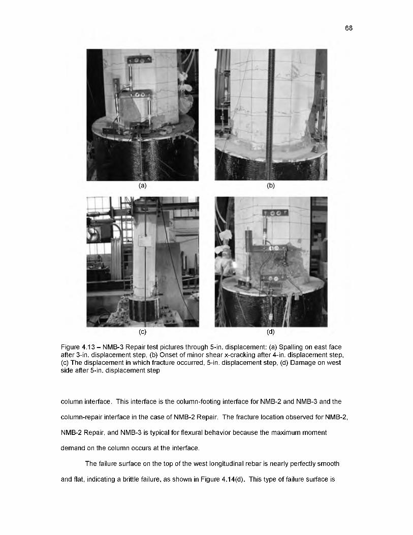
Figure 4.13 - NMB-3 Repair test pictures through 5-in. displacement: (a) Spalling on east face after 3-in. displacement step, (b) Onset of minor shear x-cracking after 4-in. displacement step, (c) The displacement in which fracture occurred, 5-in. displacement step, (d) Damage on west side after 5-in. displacement step

column interface. This interface is the column-footing interface for NMB-2 and NMB-3 and the

column-repair interface in the case of NMB-2 Repair. The fracture location observed for NMB-2,

NMB-2 Repair, and NMB-3 is typical for flexural behavior because the maximum moment

demand on the column occurs at the interface.

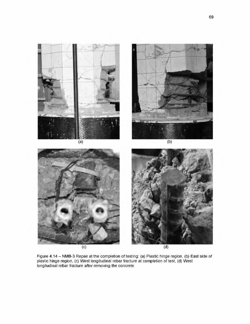
The failure surface on the top of the west longitudinal rebar is nearly perfectly smooth

and flat, indicating a brittle failure, as shown in Figure 4.14(d). This type of failure surface is

69

(c) (d)

Figure 4.14 - NMB-3 Repair at the completion of testing: (a) Plastic hinge region, (b) East side of plastic hinge region, (c) West longitudinal rebar fracture at completion of test, (d) West longitudinal rebar fracture after removing the concrete

70

Figure 4.15 - Typical tack weld used to connect LVDT rods to the column longitudinal rebar

characteristic of high strength, brittle metals and does not match the type of failure surface seen

in any of the previous tests. The welding is thought to have created an imperfection in the

longitudinal rebar, which was verified during testing.

The other factors contributing to the premature failure of NMB-3 Repair include the high

strength concrete on the day of testing, which was 9.33 ksi. The concrete strength during the

NMB-3 Repair test is 45% stronger than the concrete strength during the NMB-2 Repair test. The

high strength concrete increased the stiffness of the NMB-3 Repair specimen significantly when

compared to the other specimens and increased the demand on the longitudinal rebar.

The location of the GSS in NMB-2 and NMB-3 were different, causing the loading history

of the longitudinal rebar to differ. NMB-2 had the GSS located in the footing which caused the

deflection of the column to behave in a monolithic fashion. NMB-3 had the GSS located in the

column, which caused the column to deflect in a rocking manner, concentrating the plastisity

within the footing. Curvature profiles illustrate these differences in deflection characteristics

between the as-built NMB-2 and NMB-3 specimens, which are shown in Figure 4.16. The

curvature profiles for the 2-in., 4-in. and 6-in. displacement steps are shown in Figure 4.16. NMB-

3 experienced more curvature at heights above the future repair than NMB-2. This indicates that

71

-10 0 10 Curvature x 10“* (1/in.)

Figure 4.16 - Curvature profiles of NMB-2 and NMB-3

higher strains were present in the longitudinal rebar at the critical height for the repair. This

difference in loading history is not thought to be the cause of the higher fracture location in NMB-

3 Repair for a few reasons. Although NMB-3 did experience larger curvature than NMB-2 during

the as-built test at the location of the NMB-3 Repair fracture, NMB-3 also experienced larger

curvature at the typical fracture location, which is the top of the repair. From the NMB-3 Repair

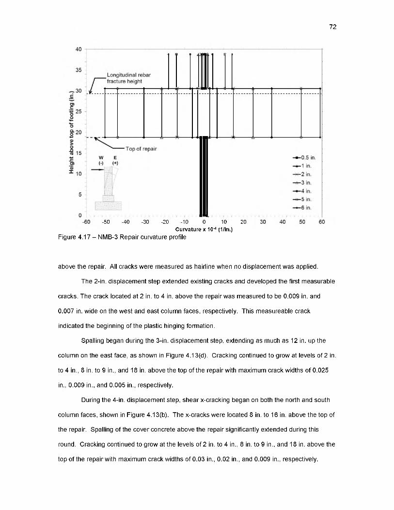
curvature profile, shown in Figure 4.17, it can be seen that the curvature just above the repair-

column interface was likely much larger than at the location of fracture. From all of these factors

it is concluded that the most likely cause of the premature longitudinal rebar fracture during the

NMB-3 Repair test was embrittlement of the longitudinal rebar due to welding of the LVDT

connection rods to the rebar.

Other notable features of the damage states of the NMB-3 Repair experienced during

testing will be explained chronologically. During the 0.5-in. displacement step no damage was

observed. The 1 -in. displacement step created two new levels of hairline cracks at 8 in. and 18 in.

above the top of the repair and opened up the crack obtained during NMB-3 test at 2 in. to 4 in.

72

-50 -40 -30 -20 -10 0 10 20Curvature x 10~* (1/in.)

Figure 4.17 - NMB-3 Repair curvature profile

above the repair. All cracks were measured as hairline when no displacement was applied.

The 2-in. displacement step extended existing cracks and developed the first measurable

cracks. The crack located at 2 in. to 4 in. above the repair was measured to be 0.009 in. and

0.007 in. wide on the west and east column faces, respectively. This measureable crack

indicated the beginning of the plastic hinging formation.

Spalling began during the 3-in. displacement step, extending as much as 12 in. up the

column on the east face, as shown in Figure 4.13(d). Cracking continued to grow at levels of 2 in.

to 4 in., 8 in. to 9 in., and 18 in. above the top of the repair with maximum crack widths of 0.025

in., 0.009 in., and 0.005 in., respectively.

During the 4-in. displacement step, shear x-cracking began on both the north and south

column faces, shown in Figure 4.13(b). The x-cracks were located 8 in. to 16 in. above the top of

the repair. Spalling of the cover concrete above the repair significantly extended during this

round. Cracking continued to grow at the levels of 2 in. to 4 in., 8 in. to 9 in., and 18 in. above the

top of the repair with maximum crack widths of 0.03 in., 0.02 in., and 0.009 in., respectively.

73

During the first cycle of the 5-in. displacement step, the extreme west longitudinal rebar

fractured in tension. The specimen at the time of fracture is shown in Figure 4.13 (c). The

fracture was very loud and expanded the spalling on the west face, shown in Figure 4.13(d).

Cracking continued to grow at levels of 2 in. to 4 in., 8 in. to 9 in., and 18 in. above the top of the

repair with maximum crack widths of 0.04 in., 0.01 in., and 0.007 in., respectively.

A decrease in load of 46% in the east direction and 12% in the west direction occurred

during the 6-in. displacement step. The cracks located at 2 in. to 4 in. and 8 in. to 9 in. above the

repair could not be measured due to the amount of spalling that had occurred. The spalling had

exposed longitudinal bars on both the east and west faces. The crack located 18 in. above the

repair closed and was measured as hairline at pause.

No new cracking or spalling occurred during the 7 in. and 8-in. displacement steps. All of

the additional damage from these cycles was through rebar straining or damage within the

confined concrete core, which could not be seen. The plastic hinge region at the end of testing is

shown in Figure 4.14.

4.4 CFRP wrap performance

The performance of the CFRP jacket used during the NMB-2 Repair and NMB-3 Repair

tests is studied in this section. The four layers of unidirectional CFRP composite provided

sufficient shear strength and confinement to the repaired cross-section, facilitating relocation of

the plastic hinge region to the top of the repair for both tests. The CFRP jacket results are highly

affected by the repair concrete properties, detailed in Section 4.1.4. The NMB-2 Repair specimen

had repair concrete, which behaved similarly to nonshrink concrete, pre-tensioning the jacket to a

strain of 0.01% prior to testing. The NMB-3 Repair specimen had repair concrete, which was

expansive, pre-tensioning the jacket to a strain of 0.15% prior to testing. The strain results from

testing will be compared to the effective strain capacities of the CFRP jackets. The effective strain

capacity for both repairs was taken as 57% of the ultimate strain capacity recorded from tensile

coupon tests (33). The CFRP strain efficiency factor accounts for strain concentrations, and the

multiaxial state of stress acting on the jacket when the CFRP wrapped member is subjected to

74

compression and bending.

4.4.1 NMB-2 Repair

The concrete that filled the NMB-2 Repair specimen’s CFRP jacket was nonshrink

concrete that pre-tensioned the jacket to 105 microstrain. This is a very small amount of pre­

tensioning, accounting for less than 2% of the jackets effective strain capacity. Transverse CFRP

cracking onset during testing at the 4-in. displacement step and grew throughout the subsequent

displacement steps, as shown in Figure 4.6. Although this characteristic is of concern, the

transverse cracking did not adversely affect the results of the repair. Additional precautions to

prevent transverse cracking in future applications of the repair are discussed in Chapter 6.

Figure 4.18 shows the uneven vertical distribution of strain throughout the CFRP jacket

during the NMB-2 Repair test. Four different levels of strain gauges, placed at different heights

above the top of the footing, are averaged together on all four sides of the CFRP jacket giving an

average top band, top, middle, and bottom strain value. The top band, top, middle, and bottom

levels of strain gauges are located 16.5 in.,14.5 in.,9.5 in., and 4.5 in. above the top of the footing

respectively. From Figure 4.18 it can be seen that the maximum strain reached in the bottom,

middle, and top levels is 15%, 38%, and 78% of the maximum strain reached in the top band

level.

Figure 4.18 shows a plateau in the strain that the wrap develops, which begins with the 4­

in. displacement step. The maximum lateral load was reached during the 4-in. displacement

step. The peak strains for each displacement step follow the shape of the response envelope

from testing, implying that the jacket strain level is controlled by load rather than displacement.

The maximum strain recorded in the jacket was on the east side of the wrap at the level of the top

band as 3200 microstrain. The effective strain capacity of the CFRP jacket is 6440 microstrain,

meaning that the jacket reached a maximum of 50% of its effective strain capacity during testing.

Uneven straining of the jacket, when displaced east and west, is shown in Figure 4.18.

The second displacement in each cycle, corresponding to a displacement in the east direction,

experiences more strain than in the first displacement. This uneven directional straining is

3000 4000Elapsed Time (sec.)

Figure 4.18 - NMB-2 Repair wrap strain gauge data averaged by height 75

76

present up to the first cycle of the 4-in. displacement step when the jacket developed the

transverse crack. The cracking relieved the uneven distribution of directional strain.

The onset of transverse cracking can be seen from individual strain gauge data from the

top band, shown in Figure 4.19. The top band east strain gauge is engaged in both of the

displacement directions through the first cycle of the 4-in. displacement step when transverse

cracking began. The onset of the transverse crack relieved the straining in both directions and

the wrap began to act similar to the top band west strain gauge, shown in Figure 4.19(a).

At the pause between displacement steps, the wrap is experiencing residual strain from dilation of

the repair concrete. It can be seen in both Figures 4.18 and 4.19 that there is a slight increase in

residual strain at the completion of each displacement step. The largest increase in residual

jacket strain is between the 1-in. and 2-in. displacement steps. This increase is due to the repair

concrete cracking, which was observed as radial cracks during testing, shown in Figure 4.8(a).

The radial cracks cause the repair concrete to dilate and increase the pressure on the CFRP

wrap, thereby increasing the wrap strain.

4.4.2 NMB-3 Repair

The repair concrete used for NMB-3 Repair was expansive concrete; the average pre­

tensioning in the CFRP jacket due to the repair concrete prior to testing was 1535 microstrain.

This is a significant amount of pre-tensioning, accounting for nearly 24% of the jacket’s effective

strain capacity. No transverse cracking occurred during testing, which was likely due in part to

the high pre-tensioning in the jacket. The pre-tensioning increases the tensile strength of the

repair concrete and alleviates the need for the CFRP to be stressed in the longitudinal direction.

The maximum strain that the wrap developed occurred during the 4-in. displacement

step, shown in Figure 4.20. The 4-in. displacement step was the last displacement step before

one of the west longitudinal bars broke. The maximum lateral load was reached during the 3-in.

displacement step. The maximum strain in the jacket during testing was 3695 microstrain at a

location 1 in. below the top of the wrap on the west side of the repair. This maximum strain is an

increase of 2160 microstrain from the pre-tensioning. The effective strain capacity of the jacket is

6440 microstrain, meaning the jacket reached 57% of its effective strain capacity.

77

Figure 4.19 - NMB-2 Repair wrap strain gauge data from top band, 3 in. below the top of therepair: (a) East, (b) West

78

Figure 4.20 - NMB-3 Repair wrap strain gauge data from top band, 3 in. below the top of therepair: (a) East, (b) West

79

In Figure 4.21 the uneven distribution of strain vertically throughout the jacket is shown.

The strain profile in Figure 4.21 is a plot of the strain gauge height above the footing versus the

maximum strain that the gauge read during a displacement step. All of the points from a given

displacement step are then connected with a dashed line due to the uncertainty in strain between

points.

The strain that the jacket experiences, as a function of distance above the top of the

footing, exponentially increases up to a height of 15 in. above the top of the footing. At 15 in.

above the top of the footing there is a discontinuity in the strain profiles. The postinstalled

headed bars extended to 15 in. above the top of the footing and are thought to be the reason for

the discontinuity in the wrap strain profiles. The mechanisms that transfer tension to the CFRP

wrap are the headed rebar and the column bearing on the expansive concrete and transferring

tension to the wrap. The discontinuity in the strain profile signifies the contribution that the

headed rebar plays in transferring tension to the wrap.

20

18

= . 160 o TO t<1)cU)

14

.E 12Oo“r= 10

o° 8o>on<C 0<DOcTO2 4 b

0.5 in. 1 in. 2 in. 3 in. 4 in.

■ /11r 'li

4 ----------------ii -----------------

ii ------------ . . . - i —

" 7

/ i ' ' Top of headed ret a r— '

; / , s ’

i/ / y

• t ' i • i 11 t i n i i 11 i i 11 0.5 in. displacement step

- - - - 1 in. displacement step

- — - 2 in. displacement step

3 in. displacement step

- - • - - 4 in. displacement step—

1500 1750 2000 3000 3250 35002250 2500 2750Microstrain (|jc)

Figure 4.21 - NMB-2 Repair west face wrap strain profile up to 4-in. displacement step

3750

80

The maximum strain that the wrap experiences at 3.875 in. above the top of the footing is

1601 microstrain. This is only a 66 microstrain increase from the pre-tensioning, an additional

1.02% of the effective strain capacity. The strain gauge located 6.875 in. above the top of the

footing only experiences a 92 microstrain increase from the pre-tensioning, an additional 1.43%

of the effective strain capacity. These numbers show the minimal strain that the wrap develops

after pre-tensioning near the top of the footing.

4.4.3 Comparison of wrap performance

The behavior of the CFRP wrap used for NMB-2 Repair and NMB-3 Repair is directly

related to the ultimate load that the system experiences. The CFRP jacket strain results for both

tests can be found in Table 4.2 along with the averaged ultimate load achieved by the specimen.

The average ultimate load is the average of the ultimate loads achieved during testing in the east

and west directions. In Table 4.2, the maximum strain recorded in the CFRP jacket is listed for

NMB-2 Repair and NMB-3 Repair from gauges located at 2 in. and 1 in. below the top of the

repair, respectively. The maximum value of strain recorded while testing NMB-2 Repair was 87%

of the maximum strain recorded in the CFRP jacket while testing NMB-3 Repair. This difference

is nearly the same as the 86% difference in average ultimate loads. This indicates that the pre­

tensioning does not significantly affect the ultimate strain that the wrap experiences; however, it

does affect the increase in strain beyond pre-tensioning that the wrap develops. The pre­

tensioning in MNB-2 Repair was only 7% of the pre-tensioning in NMB-3 Repair.

Although the pre-tensioning does not change the maximum strain within the jacket, the

pre-tensioning may influence the likelihood of transverse cracking. NMB-3 Repair did not

experience transverse cracking in the jacket even though the maximum strain values were larger.

One of the main differences regarding the CFRP wrap for NMB-3 Repair was the larger pre­

tensioning. This leads to the notion that the pre-tensioning may help to mitigate transverse

cracking by increasing the tensile strength of the repair concrete. Additional tensile strength of

the repair concrete mitigates cracking and alleviates the longitudinal stresses in the CFRP wrap.

More research is needed to determine the optimal pre-tensioning for the repair.

81

Table 4.2 - CFRP jacket strains and comparison for NMB-2 Repair and NMB-3 Repair

NMB-2 Repair NMB-3 RepairNMB-2 Repair/ NMB-3 Repair

Average ultimate load (kips) 44.6 52.1 86%

£ '3' o a■ £ (O

P ni R iar F rt FC ts

Prestressing 105 1535 7%

Maximum recorded 3200 3695 87%

Maximum increase after prestressing 3095 2160 143%

4.5 Headed rebar performance

The performance of the headed rebar used for repairing NMB-2 Repair and NMB-3

Repair will be studied in this section. The differences between the performances of the headed

rebar in the two tests will also be examined. The six no. 8 headed rebar provided sufficient

flexural strength and tension transfer between the column and footing to successfully relocate the

plastic hinge region to the top of the repair for both tests. The design and installation procedure

used for the headed bars can be found in Chapter 3. The material properties of the headed rebar

and epoxy used to anchor the headed rebar can be found in Section 4.1.

4.5.1 NMB-2 Repair

Two strain gauges were placed halfway up the free length of the headed rebar,

correlating to 7.5 in. above the top of the footing, on the extreme east and west headed bars prior

to testing. The data recorded during testing from these strain gauges is shown in Figure 4.22.

The strain gauge on the east headed rebar went off scale during the 2-in. displacement step due

to the high level of strain that the bar experienced.

The behavior of the headed rebar observed during testing seems to be influenced by the

final damage state of NMB-2. The east longitudinal rebar in the column of NMB-2 fractured

during testing, diminishing the flexural capacity of the specimen in that direction. The headed

rebar replaced this lack of flexural capacity in both tension and compression creating a moment

couple. The east headed rebar yielded in tension during the 1-in. displacement step reaching

82

-9 -8 -7 -6 -5 -4 -3 -2 -1 0 1 2 3 4 5 6 7 8 9Drift (%)

Figure 4.22 - NMB-2 Repair headed bar strain gauge data from 7.5 in. above the footing level

strains of over 1.9 times the yield strain during this displacement step. After the 1 -in.

displacement step the east strain gauge was lost. It is assumed that the east headed bar went

well beyond 1.9 times the yield strain in subsequent displacement steps. The west headed rebar

yielded in compression during the 3-in. displacement step, reaching compressive strains of nearly

2.8 times the yield strain during the 7-in. displacement step.

4.5.2 NMB-3 Repair

The strain gauge data from 7.125 in. above the top of the repair on the west extreme

headed rebar and 6.5 in. above the top of the footing on the east extreme headed rebar are

shown in Figure 4.23 versus both drift and lateral load. From Figure 4.23 it can be seen that the

headed rebar at these two locations reached up to 50% of the yield strain during testing. When

looking at the strain data plotted versus load it can be seen that the headed rebar acted linearly

with a different stiffness in compression and tension. This linear relationship with load remains

83

-60 -40 -20 0 20 40 60Load (kips)

(b)

Figure 4.23 - NMB-3 Repair headed bar strain gauge data from west gauge 7.125 in. above the footing level and east gauge 6.5 in. above the footing level plotted versus: (a) Drift, (b) Load

84

constant throughout the test since the headed rebar remained elastic. The east headed rebar

appears to have more strain than the west headed rebar, partially due to the gauge being located

closer to the footing on the east rebar.

There were six strain gauges placed on the extreme west headed rebar located at 1 in,

4.25 in., 7.125 in., 8.375 in., 10.5 in., and 14.5 in. above the top of the footing. The maximum

strain during the 0.5-in. through 4-in. displacement steps in tension and compression is plotted

versus the distance from the top of the footing in Figure 4.24. These strain profiles show that the

highest strains in the headed rebar occur at the repair-footing interface. This is reasonable since

this is the location with the maximum development length and maximum moment demand. There

is a large variation in the strain profiles for the displacement steps up to 2 in., which is due to the

large difference in the maximum load during those displacement steps. The envelope curve of

NMB-3 Repair, in Figure 4.11, shows that the maximum load starts to form a plateau at the 2-in.

displacement step.

4.5.3 Comparison of headed rebar performance

Unlike the CFRP wrap performance, the headed rebar performance does not seem to

follow a trend between NMB-2 Repair and NMB-3 Repair. Although NMB-3 Repair reached a

higher ultimate load than NMB-2 Repair, the headed bars were strained much less in NMB-3

Repair. At the midheight of the headed bar length above the top of the footing, the maximum

strains recorded in the NMB-2 Repair and NMB-3 Repair tests were 1.9 and 0.44 times the yield

strain, respectively. Furthermore the maximum strain gauge reading, of 1.9 times the yield strain,

for NMB-2 Repair occurred during the 1-in. displacement step and likely experienced much higher

strains in subsequent displacement steps. However, it would be expected that NMB-3 Repair

would experience somewhat less demand on the headed rebar due to the higher column and

footing concrete strength and the higher repair concrete strength.

The extreme east longitudinal rebar was fractured in the as-built column during both the

NMB-2 Repair and NMB-3 Repair tests. This deficiency in the as-built column can be clearly

seen during the NMB-2 Repair test due to the large moment couple that the headed bars provide

85

16

1 4

0ot© 12

10

K A - - * ■ - 0 . 5 i n . d i s p l a c e m e n t s t e p

- - x - - 1 i n . d i s p l a c e m e n t s t e p

2 i n . d i s p l a c e m e n t s t e p

-

" \" V i ' \ i i \ *

VX

%■, %

\ \I v i i » * a it i i

\ \ - - o - -

— »—

3 i n . d i s p l a c e n

4 i n . d i s p l a c e n

n e n t s t e p

n e n t s t e p

i ti i i i

i i • v ' v

\

\\

>

V v

N N1\ \

" SX11 • t

1!1

t\\\*

\11 t

1

11it

11111

s

11t

0 . 5 i n .

N %S K

1 i n . 2 n - 3 i n .

i n .

op

o° 6 0 > o.Qro 4oocrowQ

2 0 0 4 0 0 6 0 0 8 0 0 1 0 0 0

M icros tra in (|j e )

(a)

1200 1 4 0 0 1 6 0 0

1 6

=3 - 1 4

0 oto 12

10oo

ou 60>on(S 4

0 o cCS « 2b

1

0 . 5 i n . d i s p l a c e m e n t s t e p

1 i n . d i s p l a c e m e n t s t e p

2 i n . d i s p l a c e m e n t s t e p

- - 0 - - 3 i n . d i s p l a c e m e n t s t e p

4 i n . d i s p l a c e m e n t s t e p

i )■

S

s * * * *■

/

' O r J "

' s ' * " /

"*» . \

/ / •" /

//ri

\v S

S S ^ S ' s

\

V■ -w '•

\

\ \

' < * >

„ j# ;i

/

f r

- ^*

s*

**

w

1/

td

/i

//

I1

1

*111

\\\\

iIlii

f/

d O

4 i n . 3 i

11

1

i . 2 i n .

\\

*

1 i n .

iI*

0 . 5 i n

- 7 0 0 - 6 0 0 - 5 0 0 - 4 0 0 - 3 0 0 - 2 0 0 - 1 0 0 0 1 0 0 2 0 0

M icros tra in (lie)

(b)Figure 4.24 - NMB-3 Repair west headed rebar strain profile up to 4-in. displacement step: (a) Tension, (b) Compression

86

when the specimen is displaced to the west. However, the headed rebar shared the load

symmetrically between the west and east sides during the NMB-3 Repair test.

The repair concrete, which had drastically different properties between NMB-2 Repair

and NMB-3 Repair, may play a large role in the behavior of the headed rebar. The repair

concrete in NMB-2 Repair was nonshrink, and in NMB-3 Repair the repair concrete was

expansive. As mentioned previously, the increased pre-tensioning of the CFRP jacket for NMB-3

Repair increased the tensile strength of the repair concrete significantly. The amount of tension

that is transferred to the headed bars would be significantly decreased when the repair concrete

can take much of the tensile load. The pre-tensioning in NMB-3 Repair also increases the

compressive strength of the repair concrete significantly, which reduces the demand on the

headed rebar. The expansive repair concrete used for NMB-3 Repair is thought to be the main

reason that the demand on the headed rebar during the NMB-3 Repair test was much less than

during the NMB-2 Repair test.

4.6 Comparison of tests

To understand the performance of the repair tests, the results must be compared to the

as-built tests. This is a comparison between the cyclic performance of a precast concrete

column-to-footing assembly where the column is connected to the footing using GSS connections

and the subsequent repair. Also, the results from the NMB-2 Repair and NMB-3 Repair tests

must be compared to understand the advantages and disadvantages of the design decisions

made between the two. This section will compare the results of NMB-2, NMB-2 Repair, NMB-3,

and NMB-3 Repair in terms of the overall system performance, energy dissipation capacities, and

stiffness degradation characteristics.

4.6.1 System performance

The system performance of all the tests in terms of lateral load capacity, displacement

capacity, displacement ductility, and energy dissipation capacity is shown in Table 4.3. It can be

seen that the repair tests had approximately 30% larger lateral load capacities than the as-built

87

Table 4.3 - Performance evaluation criteria comparison

Performance evaluation criterion NMB-2

NMB-2Repair NMB-3

NMB-3Repair

NMB-2 Repair / NMB-2

(%)

NMB-3 Repair / NMB-3

(%)

NMB-2 Repair / NMB-3 Repair

(%)

Late

ral

load

ca

paci

ty

(kip

s)

East 37.8 44.4 39.9 51.0 118 128 87

West -31.9 -45.6 -41.2 -53.6 143 130 85

Average 34.3 44.6 40.6 52.1 130 128 86

Dis

plac

emen

tca

paci

ty(in

.)

East 6.61 6.68 7.83 4.41 101 56 151

West -6.00 -6.69 -7.33 -5.66 111 77 118

Average 6.42 6.68 7.59 4.64 104 61 144

Dis

plac

emen

tdu

ctili

ty

East 6.44 7.52 6.66 3.86 117 58 195

West 5.39 4.15 6.90 3.88 77 56 107

Average 6.10 5.95 6.79 3.66 98 54 162

Cum

ulat

ive

ener

gy

diss

ipat

ion

(kip

-in.)

4 in. displacement

step573 654 301 696 114 231 94

Total 1563 2240 2753 1114 143 40 201

tests. This increase in load capacity is thought to be due to two reasons. First, the moment arm

for the repair tests is decreased by nearly 20% due to the height of the repair and therefore, a

larger load is required to achieve a plastic hinge. Second, the repair tests occurred after the as-

built tests and therefore, the concrete compressive strength of the as-built concrete was always

larger.

The displacement capacity of NMB-2 Repair is slightly greater than the displacement

capacity of NMB-2. This is an interesting trait because the repair should have a decreased

displacement capacity due to the shortened column length. This truncated column means that for

a given displacement the repair will have a larger rotational demand than the as-built. However,

the as-built is a precast specimen using GSS as the connection and the displacement capacity

may be adversely affected due to slip. The repair transforms the precast specimens into systems

that perform more like monolithic assemblies in terms of curvature. NMB-3 Repair did not have

88

as much displacement capacity as NMB-3 due to the longitudinal rebar fracture occurring during

the 5-in. displacement step. This fracture is thought to be an anomaly due to a flaw in the rebar

from welding.

The averaged displacement ductility of NMB-2 Repair, 5.95, is nearly identical to the

displacement ductility of NMB-2, which was 6.10. NMB-3 Repair did not achieve large

displacement ductility values due to the longitudinal rebar fracture. However, from the NMB-2

Repair test it can be seen that the repair is capable of restoring the diminished load and

displacement and displacement ductility capacities of the precast specimens, which have

experienced large amounts of earthquake induced damage.

Another useful comparison is to superimpose the hysteretic responses of the as-built and

repair tests, as shown in Figure 4.25. From Figure 4.25(a) it can be seen that the NMB-2 Repair

hysteresis is at higher values of load for all displacements than the NMB-2 hysteresis. This is an

indication that NMB-2 Repair is dissipating more energy at all displacement steps. The NMB-3

Repair hysteresis is very stiff during the cycles prior to the longitudinal rebar fracture, as shown

by the difference from the NMB-3 hysteresis. After the bar fracture, the hysteretic response is

highly degraded. This degradation is primarily when NMB-3 Repair is displaced to the east. The

hysteretic loops of NMB-3 Repair in the west direction of testing never fall below the hysteretic

response of NMB-3.

All four tests can be easily compared using the force-displacement response envelopes,

shown in Figure 4.26. From Figure 4.26 it can be seen that the repaired specimens achieve

higher load values for each displacement step than the as-built specimens. The only exception to

this is NMB-3 Repair in the east direction of testing after the longitudinal rebar fractured. Also, it

can be seen from Figure 4.26 that the initial stiffness of the repaired specimens is larger than the

as-built tests, due to the smaller column length.

The curvature profiles up to the 4-in. displacement step from the NMB-2 Repair and

NMB-3 Repair tests are shown in Figure 4.27. From this plot, the curvature below the top of the

repair, prior to transverse cracking of the CFRP jacket in NMB-2 Repair, was larger during the

NMB-3 Repair test. However, the curvature just above the repair was larger during the NMB-2

89

Figure 4.25 - Overlapping as-built and repair hysteresis: (a) NMB-2 and NMB-2 Repair, (b) NMB- 3 and NMB-3 Repair

90

Drift (%)Figure 4.26 - As-built and repair testing response envelopes

-45 -30 -15 0 15Curvature x 10-4 (1/in.)

Figure 4.27 - Curvature profiles for NMB-2 Repair and NMB-3 Repair

Force

(K

N)

91

Repair test than during the NMB-3 Repair test. The smaller curvature in NMB-3 Repair just

above the repair indicates that curvature was spread to higher column sections. This curvature

demand at higher sections was highlighted by the longitudinal rebar fracturing 10.5 in. above the

top of the repair in NMB-3 Repair versus 3 in. above the top of the repair during NMB-2 Repair.

4.6.2 Energy dissipation capacity

The cumulative energy dissipation curves for NMB-2, NMB-2 Repair, NMB-3, and NMB-3

Repair is shown in Figure 4.28. The energy dissipation at the completion of each displacement

step was calculated for each specimen and summed with previous displacement steps to obtain

the cumulative energy dissipation values. The ultimate displacement of each specimen is marked

by an X on the cumulative energy dissipation curve. When the ultimate displacement occurred

between displacement steps, linear interpolation was used to obtain the total energy dissipation

value, as listed in Table 4.3.

3 4 5Displacement step (in.)

Figure 4.28 - Cumulative energy dissipation capacity of four tests

92

From Figure 4.28 it can be seen that both repairs dissipate more energy at each

displacement step than the as-built specimens. NMB-2 Repair has a cumulative energy

dissipation capacity equal to 143% of the cumulative energy dissipation capacity of NMB-2. Since

the ultimate displacement of NMB-3 Repair is very low due to the premature longitudinal rebar

fracture, the cumulative energy dissipation capacity of NMB-3 Repair is only 40% of the

cumulative energy dissipation capacity of NMB-3. However, when the cumulative energy

dissipation of all four tests is compared at the completion of the 4-in. displacement step, NMB-3

Repair dissipates the most energy. NMB-3 Repair dissipates 231% of the energy that NMB-3

had dissipated at the completion of the 4-in. displacement step.

4.6.3 Stiffness degradation

The stiffness degradation curves for NMB-2, NMB-2 Repair, NMB-3, and NMB-3 Repair

are shown in Figure 4.29. To allow comparison between the as-built and repaired specimens the

stiffness of each test has been normalized to the initial stiffness. The initial stiffness for each

specimen, found in Table 4.4, is the stiffness during the 0.5-in. displacement step. It is known

that the repaired specimens will have higher stiffness than the as-built specimens due to the

shortened column length. Therefore, to provide a comparison of the stiffness degradation

characteristics of all the tests, the normalization was made. The ultimate displacement of each

specimen is marked by an X on the stiffness degradation curve.

From Figure 4.29 it can be seen that the repaired specimen’s exhibit higher normalized

stiffness at each displacement step compared to the as-built specimens, prior to the ultimate

displacement. NMB-3 Repair has much less stiffness degradation, up to the 4-in. displacement

step, than any of the other specimens. The stiffness of NMB-3 Repair degrades rapidly between

the 4-in. and 5-in. displacement step due to the longitudinal rebar fracturing. After the 4-in.

displacement step NMB-3 Repair’s normalized stiffness is very close to the normalized stiffness

of the other three specimens. NMB-2 Repair and NMB-2 demonstrate very similar stiffness

degradation characteristics throughout all of the displacement steps prior to the ultimate

displacement.

Stiff

ness

no

rmal

ized

to 0.5

in.

dis

plac

emen

t st

ep

93

Displacement step (in.) Figure 4.29 - Stiffness degradation of all four tests

Table 4.4 - Initial stiffness values

TestInitial Stiffness

(kip/in.)

NMB-2 40.8

NMB-2 Repair 42.9

NMB-3 44.4

NMB-3 Repair 45.3

94

4.6.4 Conclusions

The comparisons from Section 4.6 have shown that the repair procedure developed in

this study is capable of restoring the capacities of cyclically damaged precast concrete bridge

column-to-footing assemblies to levels equal to the undamaged performance in terms of lateral

load capacity, displacement capacity, displacement ductility, and cumulative energy dissipation

capacity. The damage state of the specimens prior to repair was severe, including longitudinal

rebar fracture for both specimens. From these results it can be seen that the repair is capable of

achieving the desired performance, which was to emulate the performance of the as-built

specimen, making the repair an attractive alternative to replacing damaged bridges following an

earthquake. However, to confirm the belief that NMB-3 Repair is an outlier due to embrittled

longitudinal rebar prior to repair, more testing is needed.

CHAPTER 5

STRUT-AND-TIE MODELING

A Strut-and-Tie Model (STM) is an idealized truss model of a reinforced concrete member

where compressive forces are carried through struts and tensile forces are carried through ties.

Structural systems can be divided into two portions, B-regions where Bernoulli beam theory

applies and D-regions where the internal stress-strain distribution defies beam theory.

Disturbances in the internal stress-strain distribution, D-regions, come to an end roughly one

member-depth away from a disturbance, as defined by Saint Venant’s Principle. A disturbance is

caused by a geometric discontinuity, such as an abrupt change in cross-section, or a static

discontinuity, such as a point load. Therefore, any joint region within a structural system is

defined as a D-region. The repair procedure developed in this study induces two geometric

discontinuities: one at the repair-column interface and another at the repair-footing or repair-pier

cap interfaces. These geometric discontinuities create additional D-regions in the system due to

the abrupt changes in cross-section. STMs have been adopted as an appropriate method to

model the force distributions in D-regions (5, 12).

Two STM procedures have been developed for the as-built and repaired specimens. The

formulation of both STMs rely on the large amount of shear reinforcement provided in the as-built

specimens, preventing shear failure for both the as-built and repaired specimens. Both of the

STMs are based on a flexural failure mode as observed in testing for both the as-built and

repaired specimens. A conventional STM has been developed, which predicts the ultimate load

capacity of the assembly being modeled and associated member forces at ultimate lateral loading

conditions. This model is referred to as the conventional model because it is the STM method

outlined in ACI 318 (5) and is commonly used. Additionally, a nonlinear STM has been

96

developed, which predicts the system’s force-displacement response envelope and takes into

consideration the cyclic degradation of concrete. Both of the STM procedures were developed

using standardized modeling parameters that can be applied to different reinforcement and

geometrical layouts. Once the modeling parameters are established, the designer can use the

models to design the repair components and predict the assembly’s performance at the service

and ultimate condition.

Four specimens are modeled in this Chapter, NMB-2 Repair and NMB-2, which are

described in Chapters 2-4, as well as LEN-2 Repair and LEN-2. The details pertaining to LEN-2

Repair and LEN-2 are not covered in this document. Detailed descriptions, test results, and

analysis for LEN-2 and LEN-2 Repair are the subjects of other studies (2, 34). LEN-2 is a

column-to-pier cap specimen that is connected using a GSS manufactured by Lenton Interlock.

The GSS cast in the pier cap of LEN-2 uses grout to secure the field dowel and threads to secure

the bar cast into the concrete. The GSS are located in the pier cap, which is dimensioned 9 ft.

long, 2 ft. wide, and 2 ft. tall. The geometry and reinforcement in the column is identical to NMB-

2. LEN-2 was tested at the same lab and under the same loading protocol as NMB-2. LEN-2

Repair was repaired using the same methodology as NMB-2 Repair.

5.1 Strut-and-tie model layout

An infinite number of STM layouts are possible for a given structural system. The proper

STM layout to use is one that effectively models the force transfer mechanism of the system. As

a structural system progresses from service to ultimate loading conditions, the STM arrangement

that accurately models the force transfer mechanism changes. However, it is not possible to

change the arrangement of the model at intermediate steps when modeling. This issue is not a

concern for the conventional STM. The objective of the conventional STM is to predict the

performance at the ultimate limit state and therefore, a model that represents the force transfer

mechanism at the ultimate limit state is the most accurate model. However, the objective of the

nonlinear STM is to predict the structural performance of the system at all loading states up to the

ultimate limit state. Following the different force transfer mechanisms of the system up to the

97

ultimate limit state would yield many STM layouts, which is not possible to model. Following the

recommendations of previous research (16), a model that reflects the force transfer mechanism

at the ultimate limit state was adopted for the nonlinear STM. This decision leads to the

conventional and nonlinear STMs having the same geometrical layouts. A model reflecting a

flexural failure at ultimate loading was adopted to match the performance of NMB-2, NMB-2

Repair, LEN-2 Repair, and LEN-2. Adjustments to the formulated STM layout, which models the

laboratory loading, will have to be made to reflect the in-situ loading conditions.

The STM layout has been adapted from a previously developed conventional STM, which

modeled a column-to-pier cap assembly and the subsequent repair (34). It is critical that the

conventional STM developed is statically determinate and both internally and externally stable.

Determinacy makes the model independent of the truss member’s geometrical and material

properties, which are often difficult to obtain. An indeterminate truss is reliant upon the members

modulus of elasticity, E, and the members cross-sectional area, A, to determine the axial loads of

the truss members, assuming the system remains elastic. To achieve determinacy, the model

must satisfy eq. 5.1:

b + r = 2 j (5.1)

where b is equal to the number of truss members, r is the number of reactions, and j is the

number of joints.

The STM layout developed for NMB-2 Repair can be seen in Figure 5.1, where the

generic model inputs are labeled symbolically. Figure 5.1 will be used to help explain the generic

model layout parameters that were used to model all of the specimens in this chapter. These

generic model layout parameters were developed to be easily adapted with other specimen

configurations. It should be noted that the model in Figure 5.1 is statically determinate with 43

truss members, 3 reactions due to the simple supports at Q and W, and 23 joints. The model

reflects the loading condition during testing where external loads were applied at joints A, B, U,

and V. Joints A and B are the points of lateral and axial load application, respectively. Joints U

98

Figure 5.1 - STM layout

and V are the reactions due to the base plate at the bottom of the axial load application system.

The distributed load that the base plate applies onto the footing was idealized as two point loads

at joints U and V. The loads applied at joints U and V are each equal to half of the load applied at

B.

The model formulation of the as-built column B-region is quite simple, with three design

parameters. The angle, ©, which is measured between the axes of the diagonal strut and

transverse reinforcement. The tension force centroid at first yield, xt, and compression force

99

centroid at first yield, xc. The angle © is to remain constant between the axes of all the diagonal

struts and transverse reinforcement ties. The recommended range of values for © is between

31°-59° (16). For the given formulation the largest value of © that remained within the

recommended values was used. To determine ©, the integer number of equal length vertical

cells, x, can be manipulated until a satisfactory © value is obtained from eq. 5.2:

The correct value of x yields a © that is between 31°-59°. In Figure 5.1, x is equal to 5,

meaning there are 5 equal vertical lengths between node A and K. Hcoi is the height of the

column measured from the top of the footing to the point of lateral load application. Hrepair is the

height of the repair measured from the top of the footing to the top of the repair. For the as-built

specimens Hrepair is equal to zero. h is the width of the as-built column parallel to the direction of

lateral loading.

The tension and compression force centroids at first yield, xt and xc respectively, are

found from a sectional analysis of the as-built column. The first yield state is defined by the onset

of the extreme tension steel yielding or the extreme concrete compression fiber reaching a strain

value of 0.002 in./in. (16). Once xt and xc are determined, the nodes on the compression face of

the as-built column are located a distance xc away from the edge of concrete, and the nodes on

the tension face of the as-built column are located a distance xt away from the edge of the

column concrete in tension, as shown in Figure 5.1. The distance from the extreme concrete

compression fiber to the neutral axis, c, at first yield should be recorded at this stage. Any

reinforcement located within the tension zone at first yield, as shown in Figure 5.2, will contribute

to the associated tie area.

Similarly, the tension and compression force centroids of the repair at first yield, xt’ and

xc‘ respectively, are found from a sectional analysis of the repair cross-section. The confined

compressive strength of the concrete within the repair, fcc’, should be used due to the high

(5.2)

100

Figure 5.2 - Graphical representation of first yield state

confinement that the CFRP wrap provides. An accurate prediction of fcc’ can be determined from

previous research (35) or can be conservatively taken as 1.5fc’ (6). The contribution of the as-built

column steel is neglected in the repair sectional analysis due to the damage state of the

longitudinal steel. Once xt’ is determined, the nodes and corresponding ties that represent the

contribution of the headed rebar (nodes L, O and S, in Figure 5.1) are located a distance xt’ away

from the edge of repair. Any headed rebar located within the tension zone at first yield, as shown

in Figure 5.2, will contribute to the headed rebar tie area.

The compression force centroid in the repair, xc’, is used to locate the node that transmits

the compressive forces from the repair into the footing (node R in Figure 5.1). This node is

located a distance xc’ away from the edge of the repair and at the height of the top longitudinal

rebar tie in the footing. The distance from the extreme concrete compression fiber to the neutral

axis, c’, at first yield should be recorded at this stage. The height of the CFRP tie from the top of

the footing, H CFrp , was determined from the strain profiles recorded during the NMB-3 Repair

test, as shown in Figure 4.20. The centroid of the tensile force for the 1-inch displacement step

strain profile was used to determine H C frp . The 1-inch displacement step strain profile was used

since first yield occurs between the 0.5-inch and 1-inch displacement steps. The H C frp

101

calculated from the strain profile was 12.5 in. above the top of the footing, correlating to 70% of

Hrepair.

The height that the headed rebar terminates below the top of the footing, Hheaded in Figure

5.1, is equal to the embedment length of the headed rebar minus half of the epoxy anchorage

development length. Anchorage of ties at half of the bond length has been used in previous

studies (36). The node at the top of the headed rebar is located at the location of the head. This

is due to the drastically shortened development length of headed rebar (15).

The tie representing the longitudinal as-built column rebar was terminated above the

GSS interface because the STM developed is for an as-built condition in which longitudinal rebar

fracture occurred. The rule for anchoring the reinforcement half way up the development length

of the tie does not apply to the longitudinal rebar in the as-built column due to the high clamping

forces the CFRP wrap provide. The logical place for termination of the as-built column

longitudinal rebar tie is at the intersection of the longitudinal rebar and the strut that connects the

headed rebar to xc’ (node P in Figure 5.1). This location provides anchorage for the longitudinal

column rebar from struts developed in the headed rebar, CFRP wrap, and as-built column. This

strong anchorage matches test data from NMB-2 Repair where the as-built column longitudinal

rebar fractured 21.5 in., 50% of the design development length, above the fracture location from

the NMB-2 test. This short development length implies that there was significant clamping force

on the longitudinal rebar, which is represented in the STM by the anchorage struts.

All of the ties in the STM layout must correlate to the actual reinforcement arrangement,

which consists of transverse and longitudinal steel. There is no tensile capacity in the concrete at

the ultimate limit state. Also, longitudinal ties in the footing should be located at the centroid of

the rebar for positive and negative moment steel.

An axial load, Paxial, is applied to the model that replicates the axial load applied during

testing. During testing, Paxiai was applied through an actuator resting on the top of the column.

This actuator pushed against a steel beam, which transferred Paxial to the footing or pier cap

through high strength rods. To replicate this loading scenario, Paxial is applied downward at node

B on Figure 5.1, and the reactions are applied at nodes U and V upward, as shown in Figure 5.1.

102

Each node U and V is loaded with half of Paxial in the upward direction and replicates the bearing

plate, which transferred the load to the footing or pier cap. More detailed schematics and pictures

of the axial load apparatus can be found in Chapter 2.

The conventional STM developed is a general design procedure used to predict the

ultimate load capacity of a column-to-footing or column-to-pier cap assembly. The conventional

STM developed is a determinate truss model that does not rely on the geometrical or material

properties of the members. Thus, modeling can be carried out by hand or with any structural

analysis package capable of analyzing a truss.

5.2.1 Allowable design forces

The design procedures adopted by ACI (5) were used for the formulation of the

conventional STM. The allowable concrete stress of a strut, fce, is given by eq. 5.3:

where ps is equal to 0.75 for bottle shaped struts with adiquate transverse reinforcement. The

allowable concrete stress on the face of a nodal zone, fce, is given by eq. 5.4:

where, pn is equal to 1.0 for nodes not anchoring any ties, 0.80 for nodes anchoring one tie, or

0.60 for nodes anchoring two or more ties. From the allowable stresses given in eqs. 5.3 and 5.4,

the minimum required area of a strut, Acs, min, can be found in eq. 5.5:

5.2 Conventional strut-and-tie model

fce = 0.85 * ps * fc' (5.3)

fee = 0.85 * Pn * fc' (5.4)

A,cs,min min(0.85 * Ps * f , 0.85 * Pn * f ) (5.5)

103

where Fu is the force the strut develops in the model. Acs, min must then be checked against the

minimum available area, Acs, for the strut along its length. If Acs is less than Acs, min, the strut has

crushed, and the model cannot resist any more load. The Acs available in the cylindrical repair

section is a portion of an ellipse. In lieu of determining the area of an elliptical segment, a circular

sector of equal width can be used and the simplification will always yield a smaller Acs.

The nominal strength of a mild steel rebar tie, Fnt, in a nonprestressed member is given

by eq. 5.6:

where Ats is the cross-sectional area of steel of all the reinforcement that is in the tension zone at

first yield, which represents the tie, as seen in Figure 5.2. fy is the nominal yield strength of the

reinforcement. This indicates that a tie yielding is considered failure.

The nominal strength of the CFRP tie, Fnt, is given by eq. 5.7:

where Ats is the cross-sectional area of the CFRP jacket, calculated by multiplying Hrepair times the

thickness of the CFRP jacket. The thickness of the CFRP jacket is calculated by multiplying the

CFRP thickness per layer times the number of layers used for the repair. ffd is the effective stress

level in the CFRP jacket at failure, which can be determined from eq. 5.8:

Equation 5.8 must be less than 0.004Ef. X is the CFRP strain efficiency factor, which has

been determined experimentally, and accounts for the multiaxial state of stress acting on the

jacket and strain concentrations. It is recommended that X be taken as a value between 0.57­

0.61 (33). Conservatively, X has been taken as 0.57 for this study. If the force in the CFRP tie,

Fnt — Ats * ^ (5.6)

Fnt — A ts * ffd (5.7)

ffd = E f * -Ke * £ fu (5.8)

104

Fu, is larger than Fnt, the CFRP wrap will rupture. The minimum lateral load at which a strut

crushes, the mild steel yields, or the CFRP wrap ruptures is defined ultimate load capacity of the

system.

5.2.2 NMB-2 Repair model

All of the layout recommendations given in Section 5.1 were followed for NMB-2 Repair.

The material properties recorded on the day of test were used in the model. The layout

parameters and design inputs can be found in Table 5.1. All of the STM dimensions can be seen

in Figure 5.3. Due to the semi-expansive nature of the concrete placed within the repair, an

accurate compressive strength, fc’, on the day of testing could not be obtained. It was

determined, from concrete hammer tests, that the fc’ of the repair concrete was approximately

equal to the fc’ of the as-built concrete. Due to the uncertainty of fc’ for the repair concrete, a

conservative value of 1.5fc’ was used for fcc’. The axial load applied to the model was equal to

86.80 kips, which was the recorded value of axial load at the beginning of testing.

From these model inputs it was determined that the maximum lateral load the model

could withstand was 42.55 kips. The maximum lateral load NMB-2 Repair developed during

testing was 45.46 kips. Therefore, the model predicted the ultimate lateral load capacity to be

93.6% of the actual ultimate load achieved in the test. The model reached the ultimate load when

simultaneous yielding of the headed rebar ties LO and OS occurred, as seen in Figure 5.3. This

ultimate condition replicates the behavior observed during testing where yielding of the extreme

east headed rebar occurred during the 1 -inch displacement step. The modeling results can be

found numerically for the struts and ties in Tables 5.2 and 5.3, respectively.

The required width of each strut was determined from eq. 5.5 for Acsmin, which takes into

account the material properties as well as strut and nodal strength along the strut. Acs was then

determined for each end of the struts and checked against Acsmin. A graphical representation of

Acsmin, at a load that causes strut JK to crush, can be seen in Figure 5.4. The width required to

develop Acsmin at this load is shaded in grey. None of the struts crushed in this model, but strut

JK, which is the longitudinal strut at the column-repair interface, was at 88.6% of the struts

105

Table 5.1 - Modeling parameters used for NMB-2 Repair STMModelinput

Location/member Value

Paxial Global 86.8 kipsxc As-built column 2.5 in.

xt As-built column 5.8 in.

xc' Repair 2.9 in.

xt' Repair 4.5 in.

hCFRP Repair 12.5 in.

hheaded Footing 15.0 in.

e As-built column 50.7 deg.

fc' As-built 6.43 ksi

fcc' Repair 9.65 ksi

fy As-built long. 68 ksi

fy As-built trans. 63 ksi

fy Headed rebar 62 ksi

fu CFRP wrap 101 ksi

Figure 5.3 - NMB-2 Repair STM dimensions, loading, and reactions

106

Table 5.2 - NMB-2 Repair conventional STM strut results

M e m b e r L o c a t io n Fu (kips) Pn Acs, min ( in .2) Acs > Acs, min

AB Column 67.20@A@B

0.81.0

16.39 OK

BC Column 56.09@B@C

1.00.6

17.10 OK

BD Column 123.29@B@D

1.00.8

30.08 OK

CF Column 67.20@C@F

0.60.8

20.49 OK

DF Column 95.43@D@F

0.80.8

23.28 OK

EH Column 67.20@E@H

0.60.8

20.49 OK

FH Column 147.44@F@H

0.80.8

35.97 OK

GJ Column 67.20@G@J

0.60.8

20.49 OK

HJ Column 199.45@H@J

0.80.8

48.66 OK

IK Column 67.20@I@K

0.61.0

20.49 OK

JK Column 251.47@J@K

0.81.0

61.35 OK

KN Repair 165.78@K@N

1.00.8

26.96 OK

KP Repair 139.58@K@P

1.00.8

22.70 OK

KRRepair/Footing

101.79@K@R

1.00.8

24.83 OK

LM Repair 80.43@L@M

0.80.8

13.08 OK

LP Repair 122.04@L@P

0.80.8

19.85 OK

MO Repair 90.53@M

@O

0.8

0.618.40 OK

NRRepair/Footing

110.04@N@R

0.80.8

26.84 OK

OP Repair 90.69@O@P

0.60.8

18.44 OK

PRRepair/Footing

50.75@P@R

0.80.8

12.38 OK

QS Footing 200.11@Q@S

0.60.8

61.02 OK

RS Footing 211.43@R@S

0.80.8

51.58 OK

RV Footing 49.19@R@V

0.80.6

15.00 OK

RW Footing 108.90@R@W

0.80.8

26.57 OK

ST Footing 103.52@S@T

0.80.6

31.57 OK

SU Footing 72.80@S

@U

0.8

0.622.20 OK

107

Table 5.3 - NMB-2 Repair conventional STM tie results

M e m b e r M a te r ia l Fu (k ips) Fnt (k ips)Fu / Fnt

(%) Fnt > Fu

ACAs-built

long. rebar 52.01 268.60 19 OK

CDAs-built

trans. rebar 78.07 156.24 50 OK

CEAs-built

long. rebar 60.61 268.60 23 OK

EFAs-built

trans. rebar 42.55 156.24 27 OK

EGAs-built

long. rebar 112.62 268.60 42 OK

GHAs-built

trans. rebar 42.55 156.24 27 OK

GIAs-built

long. rebar 164.64 268.60 61 OK

IJAs-built

trans. rebar 42.55 156.24 27 OK

IPAs-built

long. rebar 216.65 268.60 81 OK

LOHeaded

rebar 146.37 146.94 100 YIELD

MN CFRP wrap 145.94 195.08 75 OK

OSHeaded

rebar 146.69 146.94 100 YIELD

QRAs-built

long. rebar 192.26 429.76 45 OK

QTAs-built

trans. rebar 41.96 99.20 42 OK

TUAs-built

long. rebar 94.63 322.32 29 OK

UVAs-built

long. rebar 36.96 322.32 11 OK

VW As-built long. rebar

60.09 322.32 19 OK

108

Figure 5.4 - Graphical representation of Acsmin for NMB-2 Repair at a fictitious load crushing JK

capacity. It should be noted that nodes M and N were moved 1.5 in. into the repair concrete to

establish the maximum allowable strut areas for KN, LM, MO, and NR. Nodes M and N are

located on the exterior of the repair concrete since they represent the CFRP wrap. If the nodes

were not relocated, the previously mentioned struts would have allowable areas equal to zero.

Due to the vast amount of confinement the wrap provides to the concrete struts located within the

wrap, the relocation of the nodes was deemed acceptable. The node relocation of M and N was

only done to calculate Acs.

109

The tie forces were checked against the available strength of each tie using the area of

reinforcement the tie represents and the associated material properties. It can be seen in Table

5.3 that only the headed rebar yield. Tie IP, which represents the longitudinal rebar in the column,

is stressed to 81% of the tie’s yield capacity.

5.2.3 NMB-2 model

All of the layout recommendations given in Section 5.1 were followed for NMB-2. The

material properties recorded on the day of the test were used in the model. The layout

parameters and design inputs can be found in Table 5.4. All of the STM dimensions are shown in

Figure 5.5. The axial load applied to the model was equal to 94.14 kips, which was the recorded

value of the axial load at the beginning of the test.

From these model inputs it was determined that the maximum lateral load the model

could withstand was 33.69 kips. The maximum lateral load NMB-2 developed during testing was

38.80 kips. Therefore, the model predicted the ultimate lateral load capacity to be 86.8% of the

actual ultimate load achieved. The model reached the ultimate load when the column longitudinal

strut LN crushed, shown in Figure 5.5. This ultimate load condition for the model replicates the

observed behavior of NMB-2 during testing where the ultimate load capacity was reached when

concrete was crushed in the column core. The column longitudinal rebar tie KO reached 82% of

its yield capacity at the failure load. The modeling results can be found numerically for the struts

and ties in Tables 5.5 and 5.6, respectively.

Table 5.4 - Modeling parameters used for NMB-2 STM____________Modelinput

Location/member Value

Paxial Global 94.1 kipsxc As-built column 2.7 in.xt As-built column 5.8 in.© As-built column 52.8 deg.fc' As-built 5.45 ksify As-built long. 68 ksi

fy As-built trans. 63 ksi

110

y i^ -12 .0 0 IN - J * -----------1 9 .3 0 I N ---------- J ^ - 12 .5 1 I N - 7k — 16 1 9 I N — J ^ -1 2 0 0 I N - j K

Figure 5.5 - NMB-2 STM dimensions, loading, and reactions

111

Table 5.5 - NMB-2 conventional STM strut results

M em b e r Location Fu (kips) Pn Acs, min (in .2) Acs > Acs, min

AB Column 56.14@A@B

0.81.0

13.70 OK

BC Column 60.04@B@C

1.00.6

18.31 OK

BD Column 114.65@B@D

1.00.8

27.97 OK

CF Column 55.76@C@F

0.60.8

17.00 OK

DF Column 91.02@D@F

0.80.8

22.20 OK

EH Column 55.76@E@H

0.60.8

17.00 OK

FH Column 135.45@F@H

0.80.8

33.04 OK

GJ Column 55.76@G@J

0.60.8

17.00 OK

HJ Column 179.89@H@J

0.80.8

43.88 OK

IL Column 55.76@I@L

0.60.8

17.00 OK

JL Column 224.32@J@L

0.80.8

54.72 CRUSH

KNColumn/Footing

55.76@K@N

0.60.8

11.34 OK

LNColumn/Footing

268.76@L@N

0.80.8

43.71 OK

MO Footing 101.69@M@O

0.80.6

31.01 OK

NO Footing 239.62@N@O

0.80.6

48.71 OK

NP Footing 47.07@N@P

0.80.6

9.57 OK

NQ Footing 93.29@N

@Q

0.80.8

15.17 OK

112

Table 5.6 - NMB-2 Repair conventional STM tie results

M em b e r M ateria l Fu (kips) Fnt (kips)Fu / Fnt

(%) Fnt > Fu

ACAs-built

long. rebar 44.90 268.60 17 OK

CDAs-built

trans. rebar 69.72 166.32 42 OK

CEAs-built

long. rebar 41.31 268.60 15 OK

EFAs-built

trans. rebar 33.69 166.32 20 OK

EGAs-built

long. rebar 85.75 268.60 32 OK

GHAs-built

trans. rebar 33.69 166.32 20 OK

GIAs-built

long. rebar 130.18 268.60 48 OK

IJAs-built

trans. rebar 33.69 166.32 20 OK

IKAs-built

long. rebar 174.62 268.60 65 OK

KLAs-built

trans. rebar 33.69 166.32 20 OK

KOAs-built

long. rebar 219.05 268.60 82 OK

MNAs-built

long. rebar 108.06 429.76 25 OK

OPAs-built

long. rebar 62.38 322.32 19 OK

PQAs-built

long. rebar62.38 322.32 19 OK

5.2.4 LEN-2 Repair model

All of the layout recommendations given in Section 5.1 were followed for LEN-2 Repair.

The material properties recorded on the day of the test were used in the model. The layout

parameters and design inputs can be found in Table 5.7. All of the STM dimensions can be seen

in Figure 5.6. Due to the semi-expansive nature of the concrete placed within the repair, an

accurate concrete compressive strength, fc’, on the day of testing was not obtained. It was

determined, from concrete hammer tests, that the fc’ of the repair concrete was approximately

113

Table 5.7 - Modeling parameters used for LEN-2 Repair STMModelinput

Location/member Value

Paxial Global 105 kips

xc As-built column 2.7 in.

xt As-built column 5.7 in.

xc' Repair 3.1 in.

xt' Repair 4.5 in.

hCFRP Repair 12.5 in.

hheaded Footing 15.0 in.

© As-built column 50.8 deg.

fc' As-built 6.00 ksi

fcc' Repair 9.00 ksi

fy As-built long. 68 ksi

fy As-built trans. 63 ksi

fy Headed rebar 62 ksi

fu CFRP wrap 101 ksi

Figure 5.6 - LEN-2 Repair STM dimensions, loading, and reactions

114

equal to the fc’ of the as-built concrete. Due to the uncertainty of fc’ for the repair concrete, a

conservative value of 1.5fc’ was used for fcc’. The axial load applied to the model was equal to

105.0 kips, which was the recorded value of axial load at the beginning of the test.

From these model inputs it was determined that the maximum lateral load the model

could withstand was 44.21 kips. The maximum lateral load LEN-2 Repair developed during

testing was 40.46 kips. Therefore, the model predicted the ultimate lateral load capacity to be

109.3% of the actual ultimate load achieved. This STM overpredicted the load capacity of the

specimen more than any other model. This is likely due to the initial condition of LEN-2 Repair

prior to cyclic testing. LEN-2 Repair was tested monotonically to a drift of 6.93% in the east

direction prior to the cyclic testing. This pushover damaged the concrete and steel making the

specimen behave in a nonsymmetrical manner when tested cyclically and degrading the LEN-2

Repaired specimen cyclic performance.

The model reached the ultimate load when the headed rebar ties LO and OW, as seen in

Figure 5.6, yielded simultaneously. The modeling results can be found numerically for the struts

and ties in Tables 5.8 and 5.9, respectively. It can be seen in Table 5.9 that tie IP, which

represents the longitudinal rebar in the column, is stressed to 81% of its capacity, and the CFRP

wrap represented by tie MN was stressed to 72% of its effective capacity. The longitudinal

column strut at the column-repair interface was at 85.8% of its capacity at failure. The same

procedure used for NMB-2 Repair was used to calculate Acs for struts KN, LM, MO, and NT.

5.2.5 LEN-2 model

All of the layout recommendations given in Section 5.1 were followed for LEN-2. The

material properties recorded on the day of test were used in the model. The layout parameters

and design inputs can be found in Table 5.10. All of the STM dimensions can be seen in Figure

5.7. The axial load applied to the model was equal to 104.0 kips, which was the recorded value

of axial load on the day of testing.

From these model inputs it was determined that the maximum lateral load the model

could withstand was 36.71 kips. The maximum lateral load LEN-2 developed during testing was

115

Table 5.8 - LEN-2 Repair conventional STM strut results

M em ber Location Fu (kips) Pn Acs, min (in.2) Ac s > Ac s, min

AB Column 69.95@A@B

0.8

1.017.06 OK

BC Column 67.74@B

@C

1.0

0.620.66 OK

BD Column 137.70@B

@D

1.0

0.833.59 OK

CF Column 69.95@C

@F

0.6

0.821.33 OK

DF Column 106.71@D@F

0.80.8

26.03 OK

EH Column 69.95@E@H

0.60.8

21.33 OK

FH Column 160.93@F

@H

0.8

0.839.26 OK

GJ Column 69.95@G@J

0.60.8

21.33 OK

HJ Column 215.14@H@J

0.80.8

52.48 OK

IK Column 69.95@I@K

0.61.0

21.33 OK

JK Column 269.35@J

@K

0.8

1.065.71 OK

KN Repair 156.33@K

@N

1.0

0.825.42 OK

KP Repair 137.59@K

@P

1.0

0.822.38 OK

KTRepair/

Pier cap130.99

@K

@T

1.0

0.831.96 OK

LM Repair 73.50@L

@M

0.8

0.811.95 OK

LP Repair 122.22@L

@P

0.8

0.819.88 OK

MO Repair 86.32@M

@O

0.8

0.617.55 OK

NTRepair/

Pier cap102.32

@N@T

0.80.8

24.96 OK

OP Repair 86.46@O

@P

0.6

0.817.58 OK

PTRepair/ Pier cap

46.12@P@T

0.80.8

11.25 OK

QX Pier cap 58.87@Q@X

0.80.8

14.36 OK

RY Pier cap 58.87@R@Y

0.60.6

17.95 OK

SW Pier cap 233.28@S@W

0.60.8

71.14 OK

TU Pier cap 64.45@T

@U

0.8

0.815.72 OK

TW Pier cap 327.86@T

@W

0.8

0.879.98 OK

TAA Pier cap 59.21@T

@AA

0.8

0.618.06 OK

TAB Pier cap 54.90@T

@AB

0.8

0.616.74 OK

UV Pier cap 32.23@U

@V

0.8

0.87.86 OK

UAC Pier cap 54.90@U

@AC

0.8

0.616.74 OK

VAD Pier cap 54.90@V

@AD

0.8

0.813.39 OK

W Y Pier cap 257.84@W@Y

0.80.6

78.63 OK

WZ Pier cap 87.36@W@Z

0.80.6

26.64 OK

XY Pier cap 38.60@X

@Y

0.8

0.611.77 OK

116

Table 5.9 - LEN-2 Repair conventional STM tie results

M em ber M aterial Fu (kips) Fnt (kips)Fu / Fnt

(%) Fnt > Fu

ACAs-built

long. rebar54.21 268.60 20 OK

CDAs-built

trans. rebar87.02 156.24 56 OK

c eAs-built

long. rebar55.93 268.60 21 OK

EFAs-built

trans. rebar44.21 156.24 28 OK

EGAs-built

long. rebar110.14 268.60 41 OK

GHAs-built

trans. rebar44.21 156.24 28 OK

GIAs-built

long. rebar164.35 268.60 61 OK

IJAs-built

trans. rebar44.21 156.24 28 OK

IPAs-built

long. rebar218.57 268.60 81 OK

LOHeaded

rebar146.66 146.94 100 YIELD

MN CFRP wrap 140.02 195.08 72 OK

OWHeaded

rebar146.93 146.94 100 YIELD

QRAs-built

long. rebar82.81 429.76 19 OK

RSAs-built

long. rebar121.41 429.76 28 OK

RXAs-built

trans. rebar44.45 262.58 17 OK

STAs-built

long. rebar263.83 429.76 61 OK

SYAs-built

trans. rebar184.76 262.58 70 OK

UABAs-built

trans. rebar44.45 219.41 20 OK

v a cAs-built

trans. rebar44.45 219.41 20 OK

YZAs-built

long. rebar139.12 429.76 32 OK

ZAAAs-built

long. rebar69.29 429.76 16 OK

AAABAs-built

long. rebar96.68 429.76 22 OK

a b a cAs-built

long. rebar64.45 429.76 15 OK

a c a dAs-built

long. rebar32.23 429.76 7 OK

117

Table 5.10 - Modeling parameters used for LEN-2 Repair STMModelinput

Location/member Value

Paxial Global 104 kipsxc As-built column 2.7 in.xt As-built column 5.7 in.© As-built column 52.5 deg.fc' As-built 6.00 ksi

fy As-built long. 68 ksi

fy As-built trans. 63 ksi

36.32 kips. Therefore, the model predicted the ultimate lateral load capacity to be 101.1% of the

actual ultimate load achieved. This slight overprediction is likely due to the failure mode of LEN-2

during the test. The specimen failed due to a combined flexure/grout pull out failure. The

conventional STM models LEN-2 as monolithic and this precast connection failure is not

accurately captured within the model. The model reached the ultimate load when the column

longitudinal strut LP crushed. The column longitudinal rebar tie KU reached 88% of its yield

capacity at the predicted ultimate load. The modeling results can be found numerically for the

struts and ties in Tables 5.11 and 5.12 respectively.

5.3 Nonlinear strut-and-tie model

The change that is made from the conventional STM to the nonlinear STM is going from

a model that appropriately simplifies the force-transfer mechanism to a model that predicts both

the force-transfer, the sequence of yielding of ties and crushing of struts, and the deflection of a

reinforced concrete system. The additional parameters required in establishing a nonlinear STM

from a conventional STM are the member areas and the material properties. The most accurate

model a designer could produce would be one that could encompass all of the reinforcement and

concrete, use the actual stress-strain material properties, and subject the model to typical seismic

ground motions. This type of modeling is very detailed, requiring a significant investment of time,

and produces challenges in even the most current Finite Element Models (FEM). The goal of the

current nonlinear STM is to establish a model that provides the designer with many of the output

118

Figure 5.7 - LEN-2 STM dimensions, loading, and reactions

119

Table 5.11 - LEN-2 conventional STM strut results

M e m b e r L o c a t io n Fu (kips) Pn Acs, min ( in .2) A cs > Acs, min

AB Column 60.37@A@B

0.81.0

15.78 OK

BC Column 65.60@B@C

1.00.6

21.44 OK

BD Column 125.84@B@D

1.00.8

32.90 OK

CF Column 60.34@C@F

0.60.8

19.72 OK

DF Column 99.84@D@F

0.80.8

26.10 OK

EH Column 60.34@E@H

0.60.8

19.72 OK

FH Column 147.72@F@H

0.80.8

38.62 OK

GJ Column 60.34@G@J

0.60.8

19.72 OK

HJ Column 195.61@H@J

0.80.8

51.14 OK

IL Column 60.34@I@L

0.60.8

19.72 OK

JL Column 243.49@J@L

0.80.8

63.66 OK

KPColumn/ Pier cap

60.34@K@P

0.60.6

19.72 OK

LPColumn/ Pier cap

291.37@L@P

0.80.8

76.18 CRUSH

MS Pier cap 46.85@M@S

0.80.8

12.25 OK

NT Pier cap 46.85@N@T

0.60.8

15.31 OK

OU Pier cap 46.85@O@U

0.60.6

15.31 OK

PQ Pier cap 57.00@P@Q

0.60.8

18.63 OK

PU Pier cap 307.59@P@U

0.60.6

100.52 OK

PV Pier cap 52.00@P@V

0.60.6

16.99 OK

PW Pier cap 45.60@P@W

0.60.6

14.90 OK

QR Pier cap 28.50@Q@R

0.80.8

7.45 OK

QX Pier cap 45.60@Q

@X

0.8

0.614.90 OK

RY Pier cap 45.60@R@Y

0.80.8

11.92 OK

ST Pier cap 30.46@S@T

0.80.8

7.96 OK

TU Pier cap 60.91@T

@U

0.8

0.619.91 OK

120

Table 5.12 - LEN-2 conventional STM tie results

M em ber M aterial Fu (kips) Fnt (kips)Fu / Fnt

(%) Fnt > Fu

ACAs-built

long. rebar47.92 268.60 18 OK

CDAs-built

trans. rebar76.61 166.32 46 OK

CEAs-built

long. rebar43.72 268.60 16 OK

EFAs-built

trans. rebar36.71 166.32 22 OK

EGAs-built

long. rebar91.61 268.60 34 OK

GHAs-built

trans. rebar36.71 166.32 22 OK

GIAs-built

long. rebar139.49 268.60 52 OK

IJAs-built

trans. rebar36.71 166.32 22 OK

IKAs-built

long. rebar187.37 268.60 70 OK

KLAs-built

trans. rebar36.71 166.32 22 OK

KUAs-built

long. rebar235.25 268.60 88 OK

MNAs-built

long. rebar67.17 429.76 16 OK

NOAs-built

long. rebar 97.62 429.76 23 OK

NSAs-built

trans. rebar35.60 352.80 10 OK

OPAs-built

long. rebar128.08 429.76 30 OK

OTAs-built

trans. rebar 35.60 352.80 10 OK

QWAs-built

trans. rebar35.60 352.80 10 OK

RXAs-built

trans. rebar35.60 352.80 10 OK

UVAs-built

long. rebar85.49 429.76 20 OK

VWAs-built

long. rebar85.49 429.76 20 OK

W XAs-built

long. rebar57.00 429.76 13 OK

XYAs-built

long. rebar28.50 429.76 7 OK

121

that would be achieved with a FEM but in a much more time efficient manner.

The nonlinear STM developed is a general design procedure used to predict the

nonlinear force-displacement response envelope for assemblies subjected to cyclic load

reversals. To accurately predict the cyclic force-displacement response envelope from the

monotonic nonlinear STM developed, material properties which take into consideration cyclic

degradation have been adopted. The model can then be used as a design aid when selecting the

proper reinforcement at service and at ultimate conditions. The nonlinear STM was run using a

nonlinear static analysis option in the computer package SAP2000. Any truss members that were

subjected to stresses that went beyond the elastic stress limit were assigned as two-joint

multilinear elastic link elements. By definition, all members in an STM are loaded uniaxialy since

it is a truss model. The elastic deflection of any given truss member, Aa, is given by eq. 5.9:

where Fu is the axial force the member is subjected to from the given loading in the model. L, E,

and A are the length, modulus of elasticity, and cross-sectional area for a given truss member,

respectively. Therefore, the displacement of the system modeled by the STM is a product of all

of the member’s uniaxial deflections. The member material properties input into the model

replace the modulus of elasticity in eq. 5.7 when the members become nonlinear. The link

elements used to model the members in the nonlinear range require a multilinear force-

displacement curve as the input. This input may be easily obtained from L, A, and the idealized

multilinear material properties.

5.3.1 Member areas

STMs by nature are made up of discrete truss members that are not allowed to overlap.

The designer’s goal in the nonlinear STM is to model the concrete strut areas as large as

possible without overlapping struts or nodes to accurately portray the rigidity provided by the

122

concrete. This design approach produces a model that is nearly solid concrete in compression

zones and comes very close to a model which can represent all of the materials in 3D space.

The strut areas in the model should be made as large as possible without overlapping

struts and while maintaining strut lengths in-between the nodes, even if this length is

infinitesimally small. This process must be done graphically for all members, except for diagonal

concrete struts in B-regions. The area of the diagonal struts in B-regions, Adc, can be found by

multiplying the perpendicular distance between the strut members by an effective web width. For

rectangular members, such as the footing and pier cap, the effective width is equal to the width of

the member. For columns that are circular, the effective width can be taken as 0.8h, where h is

the diameter of the column. Although the columns that are being modeled are octagonal, an

effective width of 0.8h was taken, conservatively. Therefore, the area of diagonal concrete struts

located in the as-built column can be found with eq. 5.10:

A d c = 2 * 0 . 8 h * s i n 0 * (h — (x c + xt) ) (5.10)

The rest of the strut areas should be found by maximizing the strut widths in 2D space.

Once the maximum possible strut widths are established in a 2D plane parallel to the lateral load

application, the strut areas can be found with the associate geometry of the system. If the strut

area changes along the length of a member, the minimum area between nodes should be used

along the entire length.

The ties used in the model can be classified as longitudinal ties and transverse ties. The

longitudinal reinforcement ties in the as-built column have an area that is equal to the area of the

longitudinal reinforcement located in the tension zone at first yield, as seen in Figure 5.2. The

longitudinal reinforcement ties representing the headed rebar have an area that is equal to the

area of the reinforcement located in the tension zone at first yield in the repair cross-section, as

seen in Figure 5.2. In the case of the footing and pier cap there are two sets of longitudinal rebar

ties, one that represents the positive moment steel and one that represents the negative moment

123

steel. The area of the CFRP wrap tie is the thickness of the wrap multiplied by the height of the

repair.

The area used for steel transverse reinforcement ties, Av, takes into consideration the

contribution of the transverse reinforcement strength, Vs, the shear strength provided by the

concrete, Vc, and the shear strength provided by an externally applied axial load, Vp. If the

transverse tie is located in the plastic hinge region, Vc should be neglected since the concrete

capacity in this case is assumed as zero. Av can be found from eqs 5.11 and 5.12 for transverse

reinforcement ties located out of the plastic hinge region and in the plastic hinge region,

respectively:

. Vs + vc + vpA V = --------- J---------- -- (5.11)

(5.12)

Vs, Vc, and Vp can be found using eqs. 5.13-5.16:

it * D'(5.13)

(5.14)

Vc = P * V V * A ve (5.15)

(5.16)

where, Vs, spirai and Vs, stirrup are the values of Vs for spiral and stirrup transverse reinforcement,

124

respectively. fvy is the yield strength of the transverse reinforcement. D’ is the concrete core

diameter measured center to center of spiral reinforcement. s is the pitch or spacing between

transverse reinforcement. © is the angle measured between the axes of the diagonal strut and

transverse reinforcement tie, as defined in Section 5.1. Avs is the shear area of transverse

reinforcement within one distance s. d is the member effective depth. p is a factor accounting for

the tensile resistance of the concrete and is computed using the Modified Compression Field

Theory (37). Ave is the effective shear area where Ave = 0.628 Ag for circular cross-sections (38).

N is the externally applied axial load, where compression is positive and tension is negative. h is

the overall width of the as-built column parallel to the direction of lateral loading, and for circular

columns h is equal to the diameter of the column. xc is the distance from the longitudinal strut in

the column to the edge of concrete, as defined in Section 5.1.

5.3.2 Member material properties

Reinforced concrete members subjected to cyclic loading, simulating earthquake loading,

experience material degradation in both the concrete and steel. Since the model is being

subjected to a monotonic load and is simulating cyclic results, the effects of the material

degradation must be taken into consideration in the material properties. The materials that are

modeled in the nonlinear STMs are concrete, CFRP confined concrete, mild steel reinforcement,

and the unidirectional CFRP wrap. All of the material properties have been simplified into linear

or bilinear stress-strain relationships for use with the model, as shown in Figure 5.8.

Two material properties Ec and the effective strut strength, fd, are required to model the

concrete struts, located outside of the CFRP jacket. A typical value of Ec was adopted for all

concrete struts and can be determined by eq. 5.17:

E c = 5 7 , 0 0 ( 5 . 1 7 )

For longitudinal concrete struts located in the B-region, fd was calculated from eq. 5.18:

125

(a) (b)

Figure 5.8 - Nonlinear STM material properties: (a) Concrete, (b) Confined concrete, (c) Mild steel, (d) CFRP

126

(max) (5.18)

where Cc(max) is the maximum flexural compression force the cross-section can develop. Cc(max) is

determined by a sectional analysis at which the extreme concrete compressive strain is at the

maximum permissible compressive strain as determined from Mander’s model (39), ecu(max), or the

extreme fiber of the tensile steel reaches a strain of 15% (18).

For concrete struts located in D-regions fd is a parameter that is still being researched. It

has been proposed that the predicted stress trajectory at the strut location prism, fan-shaped or

bottle-shaped, influences fd. Also, the given reinforcement and multiaxial state of stress play

large roles in the determination of fd. For the current study, previous values of fd established in

the literature were adopted (18) and are summarized in Table 5.13.

Generally, a value of 0.85fc’ was given to diagonal concrete struts located in B-regions. A

value of 0.51fc’ was assigned to diagonal concrete struts in potential plastic hinge regions,

diagonal struts adjacent to the column-footing joint, and longitudinal concrete struts. This value is

assigned with the understanding that these struts are very well confined by extensive steel shear

reinforcement. 0.68fc’ was assigned to all other diagonal concrete struts in D-regions.

A bilinear stress-strain relationship is used for CFRP confined concrete, which is based

on a model developed by Lam and Teng (40), as shown in Figure 5.8 (b). The model developed

by Lam and Teng for CFRP confined concrete has been adopted by ACI 440, and the governing

equations are shown in eqs. 5.19 and 5.20 (33):

f = Er * e, (5.19)

fe = f j + E2 * e c f o r e't < e c < eccu (5.20)

where the strain hardening modulus, E2, £t’, and the ultimate compressive strain in CFRP

confined concrete, eccu, are defined in eqs. 5.21-5.23, respectively:

127

Table 5.13 - D-region effective strut strength values

Effective strut strength, fd

Strut description

0.85fc'This value can be used where a prism stress

trajectory is anticipated, such as the diagonal concrete struts in the as-built column

0.68fc'This value is advised for regions of fan-shaped stress trajectories and in regions where minor

cracking is expected

0.51fc'This value is apropriate for concrete struts neighboring steel where £s is less than 1%

0.34fc'This value is the maximum stress for bottle-shaped

stress trajectories and for struts neigboring steel where £s is grater than 2%

E? =f ' - f 'Acc Lc (5.21)

£*■ = ■2 * fc '

Er - E,(5.22)

P z= P * ° C C U c C f c m (5.23)

where eccu shall not be greater than 1.0%, ec’ can be taken as 0.002, and xb is an FRP efficiency

factor, which can be taken as 1.00 for circular cross-sections. Once E2 and et’ are established, ecd

can be found by from eq. 5.24:

cdfed - fc ' (5.24)

where the effective strut strength of CFRP confined struts, fcd, is obtained from Table 5.4 with one

modification. The modification is that fd was calculated with the unconfined compressive strength

128

of the concrete, fc’, and fcd should be calculated with the confined compressive strength of the

concrete, fcc’. A conservative value of fcc’ was used equal to 1.5fc’ (6), but other expressions

could be used that are available in the literature (35). An fd value of 0.68fcc’ was used for all of the

CFRP confined concrete struts due to the semi-expansive concrete and extensive confinement.

To simplify Lam and Teng’s model into a bilinear relationship, eq. 5.19 was approximated

as linear by connecting the origin to the intersection of eqs. 5.19 and 5.20 at £t’. A new initial

modulus is assigned to the confined concrete, E1, and can be found by eq. 5.25:

f 'E x = ^ + E 2 (5.25)

The stress at which E1 and E2 intersect is designated f12. If f12 is greater than fcd, then the

confined concrete stress-strain properties become linear, making E2 irrelevant. This was the case

for both NMB-2 Repair and LEN-2 Repair, indicating the conservatism of this approach. If f12 is

less than fcd, f12 and fcd should be linearly connected following a slope of E2.

Three material properties are required to model the reinforcing steel ties in the nonlinear

STM, the elastic modulus of steel, Es, the effective yield strength of the steel, fey, and the strain

hardening ratio, s.h.r. A typical Es value for steel of 29,000 ksi was assumed for all reinforcing

steel ties. fey is dependent upon the reinforcement arrangement, location, and the properties of

the cross-section at first yield that the given tie represents. The general formula for obtaining fey

for longitudinal rebar ties is given in eq. 5.26:

fey = (5.26)Art

where T is the total tensile force in the reinforcing steel at first yield, and Art is the area of

reinforcement in the tension zone at first yield; see Figure 5.2. The reason fey has been

established is to represent the large strain gradient in reinforcing steel that can occur in column

cross-sections due to the longitudinal rebar having varying moment arms. Procedures for

129

determining the fey of circular and rectangular columns reinforced with many peripheral rebar

have been developed (18). For a typical rectangular ductile footing or pier cap with the

longitudinal reinforcement residing in a top and bottom layer, the total flexural force at first yield is

very close to the total yield strength of the reinforcement. Therefore, it is safe to assume that fey

is equal to the measured yield strength of the reinforcement in these locations. For longitudinal

ties located in D-regions, which did not originate from a B-region, fey is equal to the measured

yield strength of the reinforcement. Transverse reinforcement ties are not subjected to large

strain gradients and therefore, fey is equal to the measured yield strength of the transverse

reinforcement.

Following the recommendations of previous research (18), s.h.r.’s of 5.0% and 2.5%

were adopted for longitudinal reinforcement. For reinforcement ties with large strain gradients,

where eq. 5.26 yielded a fey value less than fy, a s.h.r. of 5.0% should be used to model the fact

that when fey is reached, not all of the reinforcement has yielded. The high s.h.r. helps model the

fact that first yield occurs long before all of the longitudinal rebar have yielded. Additionally, the

longitudinal B-region s.h.r. should be increased to 5.0% if there is not a significant amount of

transverse reinforcement (18).

The modeling parameters required to develop the stress-strain relationship for the CFRP

tie are the elastic modulus of CFRP, Ef, and the effective strain level in the CFRP jacket at failure,

£fe, where efe is defined in eq. 5.27 (33):

£fe = Ke * £fu (5.27)

£fe must be less than 0.4%. is the CFRP strain efficiency factor, which has been

determined experimentally, and accounts for the multiaxial state of stress acting on the jacket

and strain concentrations. It is recommended that be taken as a value between 0.57-0.61 (33).

Conservatively, has been taken as 0.57 for this study.

The nonlinear STM has reached its maximum applied force when the concrete crushes or

the reinforcement ruptures. Concrete crushing is defined as reaching a stress value of fd, for the

130

concrete located outside of the CFRP wrap or the CFRP confined concrete reaching a stress

value of fcd. Reinforcement rupture occurs when the mild steel or CFRP reaches a stress value

of fu of ffd, respectively.

When the nonlinear STM has reached the ultimate load due to a concrete strut crushing,

it has not necessarily reached the ultimate displacement of the system. If the model reaches an

ultimate load due to reinforcement rupturing, the model has reached the ultimate load and

ultimate displacement simultaneously. If a nonlinear STM reaches an ultimate load due to a

concrete strut crushing, the ultimate displacement can be determined by the following method.

To find the ultimate displacement of the system the displacement ductility, ^A, is

multiplied by the yield displacement, Ay. The equation used to determine is based on the

curvature ductility of the member, which can be found from a sectional analysis. For the

nonlinear STM model, is found from eq. 5.28 (27):

Mu is the ultimate moment capacity of the system, and My is the yield moment of the

system. Conservatively, an elasto-plastic assumption can be made where Mr is assumed to

equal 1.0. C is the column curvature coefficient and is equal to 1.0 or 0.5 for single and double

curvature bending, respectively. ^ is the curvature ductility of the column as defined in eq. 5.30:

5.3.3 Determination of ultimate displacement

where Mr is equal to the moment capacity ratio of the column, found from eq. 5.29:

(5.29)

131

'u(5.30)

where the ultimate and yield curvatures of the column cross-section, $u and $u, are determined

from a moment-curvature analysis of the column cross-section. Mander’s model was used to

model the stress-strain relationship of transversely reinforced concrete when determining $u and

$u (39). Also, a steel model that includes strain hardening was used to accurately portray the

steel forces at high moments. The normalized plastic hinge length for monolithic type column, Ap,

can be determined from eq. 5.31:

where Lp is the length of the plastic hinge, and Lc is the length of the column from the top of the

repair to the point of inflection. Equation 5.31 was only used for the repaired specimens that

demonstrated monolithic type curvature and damage during testing. It is known that plastic hinge

regions at precast concrete joints will not follow the plastic hinge behavior of a monolithic

counterpart. Therefore, Ap was determined experimentally for NMB-2 and LEN-2, which exhibited

plastic hinge lengths of 14 in. and 13 in., respectively. as is the reinforcement bond-slip

coefficient, which is equal to 1.0 since bond-slip in the plastic hinge region is possible, as

recommended (27). fye and dbl are the expected yield strength of the reinforcement and the

diameter of the longitudinal rebar, respectively.

It is recommended that Ay for a single curvature column be found by eq. 5.32:

(5.32)

Ay.

Once both and Ay are determined, Au can be easily established by multiplying by

132

5.3.4 NMB-2 Repair model

The nonlinear STM for NMB-2 Repair uses the same layout as the conventional STM as

shown in Figure 5.3. The member areas for the nonlinear STM ties are the same as the

conventional STM. The member areas of the struts are modified. The maximum possible strut

areas were used in the model to accurately portray the stiffness that the concrete provides. This

process must be done graphically for the D-regions to make sure that the struts fall within the

member geometry and that none of the struts or nodes overlap. A graphical representation of the

strut widths can be seen in Figure 5.9. It should be noted that nodes M and N were moved 1.5 in.

into the repair concrete to establish the maximum allowable strut areas for KN, LM, MO, and NR.

Nodes M and N are located on the exterior of the repair concrete since they represent the CFRP

wrap. If the nodes were not relocated, the previously mentioned struts would have allowable

areas equal to zero. Due to the vast amount of confinement the wrap provides to the concrete

struts located within the wrap, the relocation of the nodes was deemed acceptable.

The material properties are based on the recorded material values on the day of testing

and follow the recommendations of Section 5.3.2. Many of the material properties used in the

nonlinear STM are summarized in Table 5.14. The allowable compressive stress of concrete

struts, fd, is not included in Table 5.14 since this is a function of the strut location and adjacent

reinforcement.

The nonlinear STM force displacement results are shown in Figure 5.10 plotted over the

hysteresis recorded during testing. The nonlinear STM results can also be found in Tables 5.15

and 5.16 for the struts and ties, respectively. A summary of the events during the modeling can

be found in Table 5.17.

The ultimate load that the nonlinear STM force-displacement envelope predicted was

37.56 kip. This load is 82% of the 45.56 kip ultimate load that the specimen reached during

testing and 89% of the 42.09 kip ultimate load that the idealized average elasto-plastic response

reached. The ultimate displacement that the nonlinear STM predicted, using eqs. 5.28 and 5.31

for the displacement ductility and normalized plastic hinge length, respectively, was 5.89 in. This

predicted ultimate displacement is 81% of the ultimate displacement that NMB-2 Repair reached

133

Figure 5.9 - Strut widths used to determine the member areas of NMB-2 Repair

Table 5.14 - Selected cyclic material properties used with NMB-2 RepairMaterial

input Material Value (ksi)

Ec As-built concrete 4570

E1 CFRP conf. conc. 2520

E2 CFRP conf. conc. 469

f|2 CFRP conf. conc. 7.90

Es Reinforcing steel 29000

Ef CFRP wrap 8990

ffd CFRP wrap 57.9

134

Table 5.15 - NMB-2 Repair nonlinear STM tabular strut results

Member Material

A

(in.2)

Effective strut strength Event 1 Event 2 Event 3 Event 4

Eqn.

d4-r

s °

^4^ Fu

(kips)

fu si

f (k

/ %

fu

(

Fu(kips)

fu si

/ %

fu

(

Fu(kips)

fu si

f (k

/ %

fu

(

Fu(kips)

fu si

f (k

/ %

fu

(

AB Concrete 329

4-5.80. 5.47 46.0 0.1 2.6 56.3 0.2 3.1 57.5 0.2 3.2 59.3 0.2 3.3

BC Concrete 329 0.85 fc' 5.47 56.1 0.2 3.1 56.1 0.2 3.1 56.1 0.2 3.1 56.1 0.2 3.1

BD Concrete 329

4-5.80. 5.47 102.1 0.3 5.7 112.4 0.3 6.2 113.6 0.3 6.3 115.4 0.4 6.4

CF Concrete 329 0.85 fc' 5.47 46.0 0.1 2.6 56.3 0.2 3.1 57.5 0.2 3.2 59.3 0.2 3.3

DF Concrete 69 Cc(max) / A cs 5.85 79.0 1.1 19.5 87.0 1.3 21.5 87.9 1.3 21.7 89.3 1.3 22.1

EH Concrete 329

4-5.80. 5.47 46.0 0.1 2.6 56.3 0.2 3.1 57.5 0.2 3.2 59.3 0.2 3.3

FH Concrete 69 Cc(max) / A cs 5.85 114.6 1.7 28.3 130.5 1.9 32.2 132.4 1.9 32.7 135.2 2.0 33.4

GJ Concrete 329

4-5.80. 5.47 46.0 0.1 2.6 56.3 0.2 3.1 57.5 0.2 3.2 59.3 0.2 3.3

HJ Concrete 69 Cc(max) / A cs 5.85 150.2 2.2 37.1 174.1 2.5 43.0 176.9 2.6 43.7 181.2 2.6 44.7

IK Concrete 329

4-.510. 3.28 46.0 0.1 4.3 56.3 0.2 5.2 57.5 0.2 5.3 59.3 0.2 5.5

JK Concrete 69 0.51 fc' 3.28 185.8 2.7 81.9 217.7 3.1 95.9 221.4 3.2 97.5 227.1 3.3 100.0

KN CFRP conf. conc. 36

4-8.60. 6.56 99.2 2.8 42.0 131.5 3.6 55.6 135.3 3.8 57.3 141.0 3.9 59.7

KP CFRP conf. conc. 308

4-8.60. 6.56 88.0 0.3 4.4 113.0 0.4 5.6 116.0 0.4 5.7 120.4 0.4 6.0

KR CFRP conf. conc. 107

4-8.60. 6.56 98.3 0.9 14.1 100.0 0.9 14.3 100.2 0.9 14.3 100.5 0.9 14.4

LM CFRP conf. conc. 36

4-8.60. 6.56 48.1 1.3 20.4 63.8 1.8 27.0 65.7 1.8 27.8 68.4 1.9 28.9

LP CFRP conf. conc. 70

4-8.60. 6.56 73.0 1.0 15.8 96.8 1.4 20.9 99.6 1.4 21.6 103.8 1.5 22.5

MO CFRP conf. conc. 36

4-8.60. 6.56 54.2 1.5 22.9 71.8 2.0 30.4 73.9 2.1 31.3 77.0 2.1 32.6

NR CFRP conf. conc. 36

4-8.60. 6.56 65.9 1.8 27.9 87.3 2.4 36.9 89.8 2.5 38.0 93.6 2.6 39.6

OP CFRP conf. conc. 70

4-8.60. 6.56 54.3 0.8 11.7 71.9 1.0 15.6 74.0 1.1 16.0 77.1 1.1 16.7

PR CFRP conf. conc. 346

4-8.60. 6.56 26.6 0.1 1.2 38.3 0.1 1.7 39.7 0.1 1.7 41.8 0.1 1.8

QS Concrete 289

4-8.60. 4.37 146.2 0.5 11.6 172.3 0.6 13.6 175.4 0.6 13.9 180.0 0.6 14.2

RS Concrete 326 0.51 fc' 3.28 145.0 0.4 13.6 177.2 0.5 16.6 181.0 0.6 16.9 186.7 0.6 17.5

RV Concrete 135

4-.510. 3.28 49.2 0.4 11.1 49.2 0.4 11.1 49.2 0.4 11.1 49.2 0.4 11.1

RW Concrete 721 0.51 fc' 3.28 75.7 0.1 3.2 91.8 0.1 3.9 93.7 0.1 4.0 96.6 0.1 4.1

ST Concrete 236 0.68 fc' 4.37 83.5 0.4 8.1 93.2 0.4 9.0 94.4 0.4 9.1 96.1 0.4 9.3

SU Concrete 2624-8.60. 4.37 72.2 0.3 6.3 72.2 0.3 6.3 72.2 0.3 6.3 72.2 0.3 6.3

531

Table 5.16 - NMB-2 Repair nonlinear STM tabular tie results

Member Material

A

(in.2)

Effective yield strength Event 1 Event 2 Event 3 Event 4

Eqn.

T3or si

Of Fu(kips)

fu(ksi)

fu / fey

(%)

Fu(kips)

fu(ksi)

fu / fey (%)

Fu(kips)

fu(ksi)

fu / fey (%)

Fu(kips)

fu(ksi)

fu / fey

(%)

ACAs-built

long. rebar3 . 95 T / Art 34.1 35.6 9.0 26.4 43.6 11.0 32.4 44.5 11.3 33.1 45.9 11.6 34.1

CDAs-built

trans. rebar2 . 63 fy 63.0 64.6 24.6 39.0 71.2 27.1 42.9 71.9 27.3 43.4 73.1 27.8 44.1

CEAs-built

long. rebar3 . 95 T / Art 34.1 27.8 7.0 20.7 43.7 11.1 32.5 45.6 11.5 33.9 48.4 12.3 36.0

EFAs-built

trans. rebar2 . 63 fy 63.0 29.1 11.1 17.6 35.6 13.6 21.5 36.4 13.8 22.0 37.6 14.3 22.7

EGAs-built

long. rebar3 . 95 T / Art 34.1 63.4 16.1 47.1 87.3 22.1 64.8 90.1 22.8 66.9 94.3 23.9 70.1

GHAs-built

trans. rebar2 . 63 fy 63.0 29.1 11.1 17.6 35.6 13.6 21.5 36.4 13.8 22.0 37.6 14.3 22.7

GIAs-built

long. rebar3 . 95 T / Art 34.1 99.0 25.1 73.5 130.9 33.1 97.2 134.6 34.1 100.0 140.2 35.5 104.2

IJAs-built

trans. rebar1 . 93 fy 63.0 29.1 15.1 24.0 35.6 18.5 29.3 36.4 18.9 29.9 37.6 19.5 30.9

IPAs-built

long. rebar3 . 95 T / Art 34.1 134.6 34.1 100.0 174.4 44.2 129.6 179.1 45.3 133.0 186.2 47.1 138.3

LO Headed rebar 2.37 T / Art 49.1 87.8 37.0 75.5 116.4 49.1 100.0 119.8 50.5 102.9 124.8 52.7 107.2

MN CFRP wrap 3.40 Ef * xE * £f u 57.3 87.4 25.7 44.8 115.8 34.1 59.4 119.1 35.0 61.1 124.2 36.5 63.7

OS Headed rebar 2.37 T / Art 49.1 87.6 37.0 75.3 116.1 49.0 99.8 119.5 50.4 102.7 124.5 52.5 107.0

QRAs-built

long. rebar4 . 74 fy 68.0 138.5 29.2 43.0 164.6 34.7 51.1 167.7 35.4 52.0 172.3 36.3 53.4

QTAs-built

trans. rebar1 3 .9 fy 63.0 33.8 2.4 3.9 37.8 2.7 4.3 38.2 2.7 4.4 38.9 2.8 4.4

TUAs-built

long. rebar6 . 32 fy 68.0 76.3 12.1 17.8 85.2 13.5 19.8 86.3 13.6 20.1 87.8 13.9 20.4

UVAs-built

long. rebar6 . 32 fy 68.0 18.6 3.0 4.3 27.5 4.4 6.4 28.6 4.5 6.7 30.2 4.8 7.0

VWAs-built

long. rebar6 . 32 fy 68.0 41.8 6.6 9.7 50.7 8.0 11.8 51.7 8.2 12.0 53.3 8.4 12.4

631

137

Table 5.17 - NMB-2 Repair nonlinear STM eventsEvent 1 2 3 4 5

DescriptionLongitudinal column tie yields (IP)

Headed rebar tie yields

(LO & OS)

Longitudinal c olumn tie yields (GI)

Longitudinal column strut crushes (JK)

Ultimate displacement

is reached

Force (kip) 29 36 36 38 38Displacement (in.) 1.3 2.8 3.1 3.6 5.9

during testing. The ultimate displacement of the specimen during testing is defined as the

displacement in which a 20% decline in lateral load carrying capacity is reached.

Four ties yielded while running the nonlinear STM of NMB-2 Repair. Chronologically the

ties that yielded were the longitudinal rebar tie in the column at the repair-column interface (IP),

the headed rebar ties (LO and OS), and the longitudinal rebar tie in the column above IP (GI).

The fourth event, and the point that the maximum lateral load was reached, was when the

longitudinal concrete strut at the column-repair interface (JK) crushed. This performance

matches the observed performance during testing in terms of members that yielded and the

chronological order that they yielded in. Also, when the concrete strut crushes in the model,

event 4, the displacement approximately lines up with the displacement in which the specimen

reached its ultimate load carrying capacity. The deflected shape of the model matches the

behavior of the test results, as seen in Figure 5.11. The footing and repair remain relatively

stationary while the column deflects in both the model and the test results.

The initial stiffness of the force-displacement envelope is slightly less than that of the

testing data. Since the nonlinear STM is used to predict the degraded performance of a

specimen due to cyclic loading the last displacement during the 1-inch displacement step was

used to compare the initial stiffness. The models initial stiffness is 22.2 k/in., which is 75% of the

recorded test results.

5.3.5 NMB-2 model

The nonlinear STM for NMB-2 uses the same layout as the conventional STM as shown

in Figure 5.5. The tie areas for the nonlinear STM are the same as in the conventional STM, but

the member areas of the struts are modified. The maximum possible strut areas were used and

were determined graphically. The strut widths used in the model are shown in Figure 5.12. The

material properties used in the model are the recorded material values on the day of testing.

Pertinent material properties can be found in Table 5.4.

The nonlinear STM force-displacement results can be seen in Figure 5.13 plotted over

the hysteresis recorded during testing. The nonlinear STM results can also be found in Tables

5.18 and 5.19 for the struts and ties respectively. A summary of the events during the modeling

can be found in Table 5.20. The ultimate load that the nonlinear STM force-displacement

envelope predicted was 25.56 kips. This load is 66% of the 38.83 kip ultimate load that the

specimen reached during testing and 79% of the 32.37 kip ultimate load that the idealized

average elasto-plastic response reached. The ultimate displacement that the nonlinear STM

139

| NODE

J U STRUT

— STRUT

— TIE

Figure 5.12 - Strut widths used to determine the member areas of NMB-

predicted, using a plastic hinge length of 14 in. and eq. 5.28 for the displacement ductility, was

6.81 in. This predicted ultimate displacement is 115% of the ultimate displacement that NMB-2

reached during testing, where the ultimate displacement of the specimen during testing is defined

as the displacement in which a 20% decline in lateral load carrying capacity is reached.

One tie yielded while running the nonlinear STM of NMB-2, which was the longitudinal

rebar tie in the column at the column-footing joint (KO). The second event, and the point that the

maximum lateral load was reached, was when the longitudinal concrete strut at the column-

footing interface (LN) crushed. This performance matches the observed performance during

testing where the longitudinal rebar in the column yielded early on. Also, when the concrete strut

crushes in the model, event 2, the drift is within 1% of the drift in which the specimen reached its

ultimate load carrying capacity.

The initial stiffness of the force-displacement envelope is slightly less than that of the test

data. Since the nonlinear STM is used to predict the degraded performance of a specimen due to

cyclic loading, the last displacement during the 1-inch displacement step was used to compare

the initial stiffness. The model’s initial stiffness is 29.6 k/in., which is 113% of the recorded test

results.

140

141

Table 5.18 - NMB-2 nonlinear STM tabular strut results

Member Material

< .E

Effective strut strength Event 1 Event 2

Eqn.fd or fcd

(ksi)Fu

(kips)fu

(ksi)fu / fd (%)

Fu(kips)

fu(ksi)

fu / fd (%)

AB Concrete 335 0.85 fc' 4.71 38.0 0.1 2.4 42.6 0.1 2.7

BC Concrete 335 0.85 fc' 4.71 59.9 0.2 3.8 59.9 0.2 3.8

BD Concrete 335 0.85 fc' 4.71 96.6 0.3 6.1 101.1 0.3 6.4

CF Concrete 335 0.85 fc' 4.71 37.7 0.1 2.4 42.3 0.1 2.7

DF Concrete 77 Cc(max) / Acs 5.18 76.7 1.0 19.1 80.3 1.0 20.0

EH Concrete 335 0.85 fc' 4.71 37.7 0.1 2.4 42.3 0.1 2.7

FH Concrete 77 Cc(max) / Acs 5.18 106.7 1.4 26.6 114.0 1.5 28.4

GJ Concrete 335 .71 4.

~ O5.80. 37.7 0.1 2.4 42.3 0.1 2.7

HJ Concrete 77 Cc(max) / Acs 5.18 136.8 1.8 34.1 147.7 1.9 36.9

IL Concrete 335 0.85 fc' 4.71 37.7 0.1 2.4 42.3 0.1 2.7

JL Concrete 77 Cc(max) / Acs 5.18 166.9 2.2 41.6 181.4 2.3 45.3

KN Concrete 335 3.8<N

~ o.510. 37.7 0.1 4.0 42.3 0.1 4.5

LN Concrete 77 3.8<N

~ o.510. 196.9 2.5 90.1 215.1 2.8 98.4

MO Concrete 360 7 .7 3.

~ o8 .6 0. 68.8 0.2 5.1 77.1 0.2 5.7

NO Concrete 504 3.8<N

~ o.510. 162.0 0.3 11.4 181.7 0.4 12.8

NP Concrete 144 3.8<N

~ o.510. 47.1 0.3 11.6 47.1 0.3 11.6

NQ Concrete 504 0.51 fc' 2.83 63.1 0.1 4.4 70.7 0.1 5.0

Table 5.19 - NMB-2 nonlinear STM tabular tie results

Member MaterialA

(in.2)

Effective yield strength Event 1 Event 2

Eqn.fey

(ksi)Fu

(kips)fu

(ksi)fu / fey

(%)Fu

(kips)fu

(ksi)fu / fey

(%)

AC As-built long. rebar

3.95 T / Art 33.7 30.4 7.7 22.9 34.1 8.6 25.6

CD As-built trans. rebar

2.42 fy 63.0 58.7 24.3 38.5 61.5 25.4 40.3

CE As-built long. rebar

3.95 T / Art 33.7 12.6 3.2 9.5 19.9 5.0 14.9

EF As-built trans. rebar

2.42 fy 63.0 22.8 9.4 15.0 25.6 10.6 16.8

EG As-built long. rebar

3.95 T / Art 33.7 42.7 10.8 32.1 53.6 13.6 40.3

GH As-built trans. rebar

2.42 .03.6 22.8 9.4 15.0 25.6 10.6 16.8

GI As-built long. rebar

3.95 T / Art 33.7 72.7 18.4 54.7 87.3 22.1 65.7

IJ As-built trans. rebar

2.42 fy 63.0 22.8 9.4 15.0 25.6 10.6 16.8

IK As-built long. rebar

3.95 T / Art 33.7 102.8 26.0 77.3 121.0 30.6 91.0

KL As-built trans. rebar

1.77 fy 63.0 22.8 12.9 20.4 25.6 14.4 22.9

KO As-built long. rebar

3.95 T / Art 33.7 132.9 33.6 100.0 154.7 39.2 116.4

MN As-built long. rebar

6.32 fy 68.0 73.1 11.6 17.0 81.9 13.0 19.1

OP As-built long. rebar

4.7 4 fy 68.0 42.2 8.9 13.1 47.3 10.0 14.7

PQAs-built

long. rebar4.74 fy 68.0 42.2 8.9 13.1 47.3 10.0 14.7

142

Table 5.20 - NMB-2 nonlinear STM eventsEvent 1 2 3

Longitudinal Longitudinal UltimateDescription column tie column strut displacement

yields (KO) crushes (LN) is reachedForce (kip) 23 26 26

Displacement (in.) 0.77 1.9 6.8

5.3.6 LEN-2 Repair model

The nonlinear STM for LEN-2 Repair uses the same layout as the conventional STM as

shown in Figure 5.6. The member areas for the nonlinear STM ties are the same as the

conventional STM, but the member areas of the struts are modified. The maximum possible strut

areas were used and were determined graphically. The strut widths used in the nonlinear STM

can be seen in Figure 5.14. It should be noted that nodes M and N were moved 1.5 in. into the

repair concrete to establish the maximum allowable strut areas for KN, LM, MO, and NR. Nodes

M and N are located on the exterior of the repair concrete since they represent the CFRP wrap. If

the nodes were not relocated, the previously mentioned struts would have zero allowable areas.

Due to the vast amount of confinement the wrap provides to the concrete struts located within the

wrap the relocation of the nodes was deemed acceptable.

The material properties are obtained from the recorded material values on the day of

testing and follow the recommendations of Section 5.3.2. Many of the material properties used in

the nonlinear STM are summarized in Table 5.21. The allowable compressive stress of concrete

struts, fd, is not included in Table 5.21 since it is a function of the strut location and adjacent

reinforcement.

The nonlinear STM force-displacement results are shown in Figure 5.15 plotted over the

hysteresis and pushover recorded during testing. It should be noted that LEN-2 Repair was

tested monotonically in the east direction before it was tested cyclically. This monotonic

pushover displacement to 7% drift degraded the strength of the specimen severely in the east

direction. The nonlinear STM results can also be found in Tables 5.22 and 5.23 for the struts and

ties, respectively. A summary of the events during the modeling can be found in Table 5.24.

143

Figure 5.14 - Strut widths used to determine the member areas of LEN-2 Repair

Table 5.21 - Selected cyclic material properties used with LEN-2 RepairMaterial

input Material Value (ksi)

Ec As-built concrete 4420

Et CFRP conf. conc. 2420

E2 CFRP conf. conc. 420

fl2 CFRP conf. conc. 7.26

Es Reinforcing steel 29000

Ef CFRP wrap 8990ffd CFRP wrap 57.9

The ultimate load that the nonlinear STM force-displacement envelope predicted was

37.07 kips. This load is 79% of the 46.88 kip ultimate load that the specimen reached during the

monotonic pushover and 93% of the 40.06 kip ultimate load that the specimen reached when

tested cyclically. The ultimate displacement that the nonlinear STM force-displacement

predicted, using eqs. 5.28 and 5.31 for the displacement ductility and normalized plastic hinge

length respectively, was 5.74 in. This predicted ultimate displacement is 85% of the ultimate

displacement that LEN-2 Repair reached during the cyclic test.

-1 0 1 Drift (%)

Figure 5.15 - LEN-2 Repair hysteresis, nonlinear STM force-displacement envelope, and conventional STM load result 144

145

Table 5.22 - LEN-2 Repair nonlinear STM tabular strut results

Member Material

A

(in.2)

Effective strut strength Event 1 Event 2

Eqn.

fd or fcd (ksi)

Fu(kips)

fu(ksi)

fu / fd

(%)

Fu(kips)

fu(ksi)

fu / fd

(%)

AB Concrete 329 0.85 fc' 5.10 47.7 0.1 2.8 58.7 0.2 3.5

BC Concrete 329 0.85 fc' 5.10 67.7 0.2 4.0 67.7 0.2 4.0

BD Concrete 329 0.85 fc' 5.10 115.4 0.4 6.9 126.4 0.4 7.5

CF Concrete 329 0.85 fc' 5.10 47.7 0.1 2.8 58.7 0.2 3.5

DF Concrete 77 Cc(max) / Acs 5.23 89.4 1.2 22.3 98.0 1.3 24.5

EH Conerete 329 0.85 fc' 5.10 47.7 0.1 2.8 58.7 0.2 3.5

FH Concrete 77 Cc(max) / Acs 5.23 126.4 1.7 31.6 143.4 1.9 35.8

GJ Concrete 329 0.85 fc' 5.10 47.7 0.1 2.8 58.7 0.2 3.5

HJ Concrete 77 Cc(max) / Acs 5.23 163.3 2.1 40.8 188.9 2.5 47.2

IK Concrete 329 0.51 fc' 3.06 47.7 0.1 4.7 58.7 0.2 5.8

JK Concrete 77 0.51 fc' 3.06 200.3 2.6 85.5 234.3 3.1 100.0

KN CFRP conf. conc. 36 0.68 fcc' 6.12 90.0 2.5 40.8 122.7 3.4 55.6

KP CFRP conf. conc. 308 0.68 fcc' 6.12 85.0 0.3 4.5 110.9 0.4 5.9

KT CFRP conf. conc. 107 0.68 fcc' 6.12 123.2 1.2 18.9 127.0 1.2 19.5

LM CFRP conf. conc. 36 0.68 fcc' 6.12 45.2 1.3 20.5 61.6 1.7 27.9

LP CFRP conf. conc. 70 0.68 fcc' 6.12 70.4 1.0 16.3 95.9 1.4 22.2

MO CFRP conf. conc. 36 0.68 fcc' 6.12 49.7 1.4 22.5 67.8 1.9 30.7

NT CFRP conf. conc. 36 0.68 fcc' 6.12 58.9 1.6 26.7 80.3 2.2 36.4

OP CFRP conf. conc. 70 0.68 fcc' 6.12 49.8 0.7 11.5 67.9 1.0 15.7

PT CFRP conf. conc. 346 0.68 fcc' 6.12 21.7 0.1 1.0 33.8 0.1 1.6

QX Concrete 274 6 8 cf' 0 8 40.8 0.1 3.7 49.7 0.2 4.5

RY Concrete 274 6 8 cf' 0 8 40.8 0.1 3.7 49.7 0.2 4.5

SW Concrete 235 6 8 cf' 0 8 172.3 0.7 18.0 202.3 0.9 21.1

TU Concrete 144 0.51 fc' 3.06 44.6 0.3 10.1 54.4 0.4 12.3

TW Concrete 216 0.51 fc' 3.06 224.9 1.0 34.0 275.7 1.3 41.7

TAA Concrete 90 0.51 fc' 3.06 59.2 0.7 21.5 59.2 0.7 21.5

TAB Concrete 242 0.51 fc' 3.06 38.0 0.2 5.1 46.3 0.2 6.2

UV Concrete 144 0.51 fc' 3.06 22.3 0.2 5.1 27.2 0.2 6.2

UAC Concrete 242 0.68 fc' 4.08 38.0 0.2 3.8 46.3 0.2 4.7

VAD Concrete 242 6 8 cf' 0 8 38.0 0.2 3.8 46.3 0.2 4.7

WY Concrete 168 6 8 cf' 0 8 194.1 1.2 28.3 225.5 1.3 32.9

W Z Concrete 72 6 8 cf' 0 8 87.4 1.2 29.7 87.4 1.2 29.7

XY Concrete 144 0.51 fc' 3.06 26.7 0.2 6.1 32.6 0.2 7.4

146

Table 5.23 - LEN-2 Repair nonlinear STM tabular tie results

Member Material

A

(in.2)

Effective yield strength Event 1 Event 2

Eqn.

"D ff )

o “

Jf Fu

(kips)fu

(ksi)fu / fey

(%)

Fu(kips)

fu(ksi)

fu / fey

(%)

ACAs-built

long. rebar3.95 T / Art 33.5 36.9 9.4 27.9 45.5 11.5 34.4

CDAs-built

trans. rebar2 . 66 fy 63.0 72.9 27.4 43.5 79.9 30.0 47.7

CEAs-built

long. rebar3.95 T / Art 33.5 21.4 5.4 16.2 38.4 9.7 29.0

EFAs-built

trans. rebar2 . 66 fy 63.0 30.1 11.3 18.0 37.1 13.9 22.1

EGAs-built

long. rebar3.95 T / Art 33.5 58.3 14.8 44.1 83.9 21.2 63.4

GHAs-built

trans. rebar2 . 66 fy 63.0 30.1 11.3 18.0 37.1 13.9 22.1

GIAs-built

long. rebar3.95 T / Art 33.5 95.3 24.1 72.1 129.3 32.7 97.8

IJAs-built

trans. rebar1 . 97 fy 63.0 30.1 15.3 24.3 37.1 18.8 29.9

IPAs-built

long. rebar3.95 T / Art 33.5 132.2 33.5 100.0 174.8 44.3 132.2

LO Headed rebar 2.37 T / Art 48.9 84.5 35.6 72.9 115.1 48.6 99.4

MN CFRP wrap 3.40 Ef * x£ * £fu 57.3 80.6 23.7 41.4 109.9 32.3 56.4

OW Headed rebar 2.37 T / Art 48.9 84.6 35.7 73.0 115.3 48.7 99.5

QRAs-built

long. rebar6.32 fy 68.0 56.9 9.0 13.2 69.7 11.0 16.2

RSAs-built

long. rebar6.32 fy 68.0 83.6 13.2 19.5 102.2 16.2 23.8

RXAs-built

trans. rebar6 . 29 fy 63.0 30.8 4.9 7.8 37.5 6.0 9.5

STAs-built

long. rebar6.32 fy 68.0 188.8 29.9 43.9 225.8 35.7 52.5

SYAs-built

trans. rebar6 . 29 fy 63.0 136.4 21.7 34.4 160.3 25.5 40.4

UAB As-built trans. rebar

5 . 61 fy 63.0 30.8 5.5 8.7 37.5 6.7 10.6

VACAs-built

trans. rebar5 . 61 fy 63.0 30.8 5.5 8.7 37.5 6.7 10.6

YZAs-built

long. rebar6.32 fy 68.0 109.4 17.3 25.5 124.1 19.6 28.9

ZAAAs-built

long. rebar6.32 fy 68.0 39.6 6.3 9.2 54.2 8.6 12.6

AAABAs-built

long. rebar6.32 fy 68.0 67.0 10.6 15.6 81.6 12.9 19.0

ABACAs-built

long. rebar6.32 fy 68.0 44.6 7.1 10.4 54.4 8.6 12.7

ACADAs-built

long. rebar6.32 fy 68.0 22.3 3.5 5.2 27.2 4.3 6.3

147

Table 5.24 - LEN-2 Repair nonlinear STM eventsEvent 1 2 3

Longitudinal Longitudinal UltimateDescription column tie cloumn strut displacement

yields (IP) crushes (JK) is reached

Force (kip) 30 37 37Displacement (in.) 1.4 3.0 5.7

One tie yielded while running the nonlinear STM of LEN-2 Repair, which was the

longitudinal column rebar tie at the repair-column interface (IP). The second event, and the point

that the maximum lateral load was reached, was when the longitudinal concrete strut at the

column-repair interface (JK) crushed. It can be seen in Figure 5.15 that the nonlinear STM

results match the cyclic performance of LEN-2 Repair very closely, and the conventional STM

results match the monotonic load capacity very closely. This comparison shows the applicability

of the two types of STMs. The nonlinear STM is designed to match the cyclic performance of a

system. This is achieved by entering allowable material stresses that reflect the cyclic

degradation that occurs within materials when cyclically loaded. The conventional STM is

modeled using monotonic material properties. This input is why the ultimate load of the

conventional STM matches the pushover results very closely.

5.3.7 LEN-2 model

The nonlinear STM for LEN-2 uses the same layout as the conventional STM as shown

in Figure 5.7. The member areas for the nonlinear STM ties are the same as the conventional

STM but the member areas of the struts are modified. The maximum possible strut areas were

used and were determined graphically. The strut widths used in the model can be seen in Figure

5.16. The material properties used in the model are the recorded material values on the day of

testing. Pertinent material properties can be found in Table 5.10.

The nonlinear STM force-displacement results can be seen in Figure 5.17 plotted over

the hysteresis results recorded during testing. It should be noted that the hysteretic response of

LEN-2 is affected by the bond slip, which the GSS demonstrated during testing. This

148

] NODE

STRUT

— STRUT

Figure 5.16 - Strut widths used to determine the member areas of LEN-2

characteristic pinches the hysteresis and leads to less desirable performance when compared to

NMB-2. The nonlinear STM results can also be found in Tables 5.25 and 5.26 for the struts and

ties, respectively. A summary of the events during the modeling can be found in Table 5.27.

The ultimate load that the nonlinear STM force-displacement envelope predicted was

27.78 kips. This load is 78% of the 35.68 kip ultimate load that the specimen reached during

testing and 83% of the 33.29 kip ultimate load that the idealized average elasto-plastic response

reached. The ultimate displacement that the nonlinear STM force-displacement predicted, using

a plastic hinge length of 13 in. and eq. 5.28 for the displacement ductility, was 6.22 in. This

predicted ultimate displacement is 96% of the ultimate displacement that LEN-2 reached during

testing.

149

150

Table 5.25 - LEN-2 nonlinear STM tabular strut results

Member Material

A

(in.2)

Effective strut strength Event 1 Event 2

Eqn.

fd or fcd

(ksi)Fu

(kips)fu

(ksi)fu / fd

(%)

Fu(kips)

fu(ksi)

fu / fd

(%)

AB Concrete 337 0.85 fc' 5.10 38.7 0.1 2.3 45.7 0.1 2.7

BC Concrete 337 0.85 fc' 5.10 65.6 0.2 3.8 65.6 0.2 3.8

BD Concrete 337 0.85 fc' 5.10 104.2 0.3 6.1 111.2 0.3 6.5

CF Concrete 337 0.85 fc' 5.10 38.7 0.1 2.2 45.7 0.1 2.7

DF Concrete 76 Cc(max) / A cs 5.26 82.7 1.1 20.6 88.2 1.2 22.0

EH Concrete 337 0.85 fc' 5.10 38.7 0.1 2.2 45.7 0.1 2.7

FH Concrete 76 Cc(max) / A cs 5.26 113.4 1.5 28.3 124.4 1.6 31.1

GJ Concrete 337 0.85 fc' 5.10 38.7 0.1 2.2 45.7 0.1 2.7

HJ Concrete 76 Cc(max) / A cs 5.26 144.1 1.9 36.0 160.7 2.1 40.1

IL Concrete 337 0.85 fc' 5.10 38.7 0.1 2.2 45.7 0.1 2.7

JL Concrete 76 Cc(max) / A cs 5.26 174.8 2.3 43.6 196.9 2.6 49.2

KP Concrete 337 0.51 fc' 3.06 38.7 0.1 3.7 45.7 0.1 4.4

LP Concrete 76 0.51 fc' 3.06 205.5 2.7 88.1 233.1 3.1 100.0

MS Concrete 274 0.68 fc' 4.08 30.0 0.1 2.7 35.5 0.1 3.2

NT Concrete 274 0.68 fc' 4.08 30.0 0.1 2.7 35.5 0.1 3.2

OU Concrete 274 0.68 fc' 4.08 30.0 0.1 2.7 35.5 0.1 3.2

PQ Concrete 144 0.51 fc' 3.06 36.5 0.3 8.3 43.1 0.3 9.8

PU Concrete 336 0.51 fc' 3.06 197.2 0.6 19.2 232.8 0.7 22.6

PV Concrete 48 0.51 fc' 3.06 52.0 1.1 35.4 52.0 1.1 35.4

PW Concrete 264 0.51 fc' 3.06 29.2 0.1 3.6 34.5 0.1 4.3

QR Concrete 144 0.51 fc' 3.06 18.3 0.1 4.1 21.6 0.1 4.9

QX Concrete 264 0.68 fc' 4.08 29.2 0.1 2.7 34.5 0.1 3.2

RY Concrete 264 0.68 fc' 4.08 29.2 0.1 2.7 34.5 0.1 3.2

ST Concrete 144 0.51 fc' 3.06 19.5 0.1 4.4 23.0 0.2 5.2

TU Concrete 144 0.51 fc' 3.06 39.1 0.3 8.9 46.1 0.3 10.5

One tie yielded while running the nonlinear STM of LEN-2, which was the longitudinal

rebar tie in the column at the column-pier cap joint (KU). The second event, and the point that

the maximum lateral load was reached, was when the longitudinal concrete strut at the column-

pier cap interface (LP) crushed. This performance matches the observed performance during

testing where the longitudinal rebar in the column yielded during small displacements.

The initial stiffness of the force-displacement envelope is very close to that of the test

data. Since the nonlinear STM is used to predict the degraded performance of a specimen due to

151

Table 5.26 - LEN-2 nonlinear STM tabular tie results

Member Material

A

(in.2)

Effective yield strength Event 1 Event 2

Eqn.

fey(ksi)

Fu

(kips)fu

(ksi)fu / fey

(%)

Fu(kips)

fu(ksi)

fu / fey

(%)

ACAs-built

long. rebar3 . 9 5 T / Art 33.5 30.7 7.8 23.2 36.3 9.2 27.4

CDAs-built

trans. rebar2. 4 9 fy 63.0 63.4 25.5 40.4 67.7 27.2 43.1

CEAs-built

long. rebar3 . 9 5 T / Art 33.5 9.4 2.4 7.1 20.4 5.2 15.4

EFAs-built

trans. rebar2. 4 9 fy 63.0 23.5 9.5 15.0 27.8 11.2 17.7

EGAs-built

long. rebar3 . 9 5 T / Art 33.5 40.1 10.1 30.3 56.7 14.3 42.8

GHAs-built

trans. rebar2. 4 9 fy 63.0 23.5 9.5 15.0 27.8 11.2 17.7

GIAs-built

long. rebar3 . 9 5 T / Art 33.5 70.8 17.9 53.5 92.9 23.5 70.3

IJAs-built

trans. rebar2. 4 9 fy 63.0 23.5 9.5 15.0 27.8 11.2 17.7

IKAs-built

long. rebar3 . 9 5 T / Art 33.5 101.5 25.7 76.7 129.1 32.7 97.7

KLAs-built

trans. rebar1. 8 1 fy 63.0 23.5 13.0 20.6 27.8 15.3 24.4

KUAs-built

long. rebar3 . 9 5 T / Art 33.5 132.2 33.5 100.0 165.4 41.9 125.1

MNAs-built

long. rebar6 . 32 fy 68.0 43.1 6.8 10.0 50.8 8.0 11.8

NOAs-built

long. rebar6 . 32 fy 68.0 62.6 9.9 14.6 73.9 11.7 17.2

NSAs-built

trans. rebar6. 2 3 yf 6 0 22.8 3.7 5.8 26.9 4.3 6.9

OPAs-built

long. rebar6 . 32 fy 68.0 82.1 13.0 19.1 96.9 15.3 22.6

OTAs-built

trans. rebar6. 2 3 fy 63.0 22.8 3.7 5.8 26.9 4.3 6.9

QWAs-built

trans. rebar5. 9 7 fy 63.0 22.8 3.8 6.1 26.9 4.5 7.2

RXAs-built

trans. rebar5. 9 7 fy 63.0 22.8 3.8 6.1 26.9 4.5 7.2

UVAs-built

long. rebar6 . 32 fy 68.0 54.8 8.7 12.8 64.7 10.2 15.1

VWAs-built

long. rebar6 . 32 fy 68.0 54.8 8.7 12.8 64.7 10.2 15.1

W XAs-built

long. rebar6 . 32 fy 68.0 36.5 5.8 8.5 43.1 6.8 10.0

XYAs-built

long. rebar6 . 32 fy 68.0 18.3 2.9 4.3 21.6 3.4 5.0

152

Table 5.27 - LEN-2 nonlinear STM eventsEvent 1 2 3

Longitudinal Longitudinal UltimateDescription column tie column strut displacement

yields (KU) crushes (LP) is reached

Force (kip) 24 28 28Displacement (in.) 0.82 2.5 6.2

cyclic loading, the last displacement during the 1-in. displacement step was used to compare the

initial stiffness. The models initial stiffness is 28.87 k/in., which is 99% of the recorded test

results.

5.4 Parametric study of strut-and-tie model material design values

The modeling procedures developed are intended to be used by designers who do not

have the exact material properties of the concrete, steel, or CFRP that they are modeling. Two

design procedures for material properties are examined in this study for both the conventional

and nonlinear STMs. First, nominal material properties are modeled. Nominal material

properties imply that grade 60 steel is input with a yield strength on 60 ksi and concrete ordered

from the batch plant as 6 ksi is input into the model as 6 ksi. The other design procedure

modeled is expected material properties. This is a design procedure used by designers

performing capacity based design in which underprediction of the material strength is

unconservative. Therefore, this design procedure is referred to as the seismic design material

properties. To examine the outcomes of using the differing design property procedure for both

the conventional and nonlinear STMs, NMB-2 Repair has been remodeled using nominal and

seismic design material properties.

Many suggested values exist for expected material properties for both rebar and

concrete. The seismic design value for the yield strength of steel used in this study is 1.25fy (5),

where fy is the specified or nominal yield strength of the steel. The seismic design value for the

compressive strength of concrete used in this study is 1.1fc’, where fc’ is the specified 28-day

compressive strength. For the CFRP wrap the nominal design values were taken as the

153

manufacturer’s recommended design values, and the seismic design values were taken as the

manufacturer’s expected material properties (41).

5.4.1 Conventional strut-and-tie model

All of the layout parameters are based upon the material properties of the specimen that

is being modeled. Therefore, to model the different material properties NMB-2 Repair has a

different layout for each design procedure. The layout parameters and design inputs can be

found in Table 5.28.

The three models using differing material properties were run until a failure load was

reached. The results of the models can be found in Table 5.29. The ultimate loads achieved

were 93%, 79%, and 94% of the ultimate load reached during testing for the day of test, nominal

and seismic design material properties, respectively. Both the day of test and seismic design

models reached failure due to yielding of the headed rebar. The nominal design model failed due

to crushing on the longitudinal concrete strut at the column-repair interface.

Table 5.28 - Modeling parameters used for differing material properties for NMB-2 Repair

Modelinput Location/ member

Material PropertiesDay of Test

SeismicDesign Nominal

P axial Global 86.8 kips 86.8 kips 86.8 kips

Xc As-built column 2.5 in. 2.4 in. 2.2 in.

Xt As-built column 5.8 in. 5.9 in. 6.3 in.

Xc' Repair 2.9 in. 2.8 in. 2.3 in.

Xt' Repair 4.5 in. 4.5 in. 5.2 in.

hCFRP Repair 12.5 in. 12.5 in. 12.5 in.

hheaded Footing 15.0 in. 15.0 in. 15.0 in.© As-built column 50.7 deg. 50.7 deg. 50.9 deg.

fc' As-built 6.43 ksi 6.60 ksi 6.00 ksi

fcc' Repair 9.65 ksi 9.90 ksi 9.00 ksi

fy As-built long. 68 ksi 75 ksi 60 ksi

fy As-built trans. 63 ksi 75 ksi 60 ksi

fy Headed rebar 62 ksi 75 ksi 60 ksi

tf CFRP ply thickness 0.047 in. 0.04 in. 0.04 in.

fu CFRP wrap 101 ksi 123 ksi 104 ksi

154

Table 5.29 - Conventional STM results using differing material properties for NMB-2 Repair

Material properties used

Normalized to the tested Conventional ultimate load capacity

STM load (kips) (%)

Day of test 42.55 93Nominal 35.85 79

Seismic design 42.8 94

From the results it can be seen that both design philosophies provide conservative

estimates of the ultimate load capacity of NMB-2 Repair. From this analysis it appears that the

seismic design material properties more accurately predict the specimen’s performance than the

nominal design properties. This result is expected since the seismic design material properties

are closer to the tested values. However, the conventional STM does not always provide

conservative results for cyclic load capacity, as seen by the results of LEN-2 Repair and LEN-2.

Caution should be used when designing with the conventional STM since it does not account for

cyclic degradation of materials as the nonlinear cyclic STM does; see Table 5.13.

5.4.2 Nonlinear strut-and-tie model

The nonlinear STM of NMB-2 Repair was run for the two different material strength

design procedures and compared to the results obtained using the material properties from the

day of testing. The same layout parameters were used for the nonlinear STM as the conventional

STM and can be found in Table 5.28. Additional material values were input into the nonlinear

model following the recommendations of Section 5.3.2 and are summarized in Table 5.30. The

results from the three simulations can be found in Table 5.31 and seen in Figure 5.18.

All of the models underpredicted the ultimate load capacity of the specimen. When compared to

the ultimate load of the idealized elasto-plastic response of NMB-2 Repair the day of test,

nominal, and seismic design ultimate load capacities were 89%, 64%, and 92% of the peak

elasto-plastic load, respectively. The ultimate displacement capacities of the three simulations

were 88%, 83%, and 91% of the tested ultimate load capacity for the day of test, nominal, and

seismic design simulations respectively. There was one event when running the nonlinear STM

using nominal design values, which was crushing of the longitudinal concrete strut at the column-

155

Table 5.30 - Selected cyclic material properties used for NMB-2 Repair design proceduresMaterial Properties (ksi)

Materialinput Material Day of Test

Seism icDesign Nominal

Ec As-built concrete 4571 4631 4415

Ei CFRP conf. conc. 2520 2552 2411

E2 CFRP conf. conc. 469 473 407

fl2 CFRP conf. conc. 7.90 8.10 7.22

Es Reinforcing steel 29000 29000 29000

Ef CFRP wrap 8990 10200 9450

ffd CFRP wrap 57.9 69.8 52.8

£u (%)CFRP tensile

elongation1.13% 1.12% 0.98%

Table 5.31 - Results from NMB-2 Repair parametric study

Model

Ultimate loadModel Test max Test elasto-plastic (kips) (kips) (kips)

Mod el/Test(%)

Model/Test E.P. (%)

NMB-2Repair

Day of test 37.56 82 89 5.89 88Nominal 26.92 45.56 42.09 59 64 5.53 6.68 83

Seismic design 38.85 85 92 6.11 91

Ultimate displacementModel

(in.)Test Model/Test(in.) (%)

repair interface (JK). There were two events when running the nonlinear STM using seismic

design values, which was yielding of the longitudinal column rebar tie at the repair-column

interface (IP), followed by crushing of the longitudinal concrete strut at the column-repair interface

(JK). The progression of events that the seismic design model underwent replicates the

observed behavior of NMB-2 Repair during testing better than the nominal design model. Yielding

of the column rebar occurred far before the ultimate load was achieved from crushing of the

column concrete.

From these results it can be seen that the nonlinear STM underpredicts the test results in

terms of load capacity and ultimate displacement for both design procedures. The nominal

design model predicts 64% of the tested ultimate load, and the seismic design model predicts

92% of the tested ultimate load. Unlike the conventional STM, the nonlinear STM underpredicted

the ultimate load capacity for all of the tests modeled. Therefore, the most realistic design values

should be used when implementing the nonlinear STM, close to the seismic design material

properties used in this study.

156

157

5.5 Comparison of strut-and-tie model results to test data

To validate the applicability of both the conventional STM and nonlinear STM models,

various aspects of the models were compared to the recorded test results. The system as a

whole was examined in terms of global displacement and load capacity. Individual repair

components including the headed rebar and CFRP wrap were examined in detail to assess the

applicability of the STM procedure for designing the repair components.

5.5.1 System results

The conventional STM predicts the ultimate load capacity of the assembly being

modeled. These results are compared to both the ultimate load achieved during testing and the

ultimate load of the idealized elasto-plastic response, as found in Table 5.32. The nonlinear STM

produces a force-displacement response envelope of the assembly being modeled. The results

of the nonlinear STM in terms of ultimate load capacity, ultimate displacement capacity,

displacement ductility, and initial stiffness can all be compared to the test results, as summarized

in Table 5.33. The ultimate load capacity is compared to both the ultimate load achieved during

testing and the ultimate load of the idealized elasto-plastic response. The initial stiffness is

compared to the initial stiffness of the idealized elasto-plastic response curve.

All of the nonlinear STM and conventional STM results are plotted with the response

envelope of the specimen being modeled as well as the idealized elasto-plastic response, in

Figures 5.19-5.22. The response envelopes are the averaged response envelopes from both

directions of testing, and the idealized elasto-plastic responses are obtained from the averaged

response envelopes plotted. A description of the procedure used for creating the elasto-plastic

responses is given in Section 3.4.3. The displacement ductility from testing is obtained from the

average envelope idealized elasto-plastic response curves. It should be noted that an accurate

response envelope cannot be obtained for LEN-2 Repair due to the existing damage at the start

of the cyclic testing from the monotonic pushover test. Due to this fact, an idealized elasto-plastic

response cannot be generated. However, the STM results are plotted with the monotonic

Table 5.32 - Conventional STM results

ModelModel ultimate

load (kips)Test ultimate

load (kips)Test elasto-plastic

load (kips)Model/Test

(%)Model/Test

E.P. (%)

NMB-2Repair

Day of test 42.55 93 101

Nominal 35.85 45.56 42.09 79 85

Seismic design 42.80 94 102

NMB-2 33.69 38.83 32.37 87 104

LEN-2 Rep 44.21 40.46 - 109 -

LEN-2 36.71 36.32 33.29 101 110

Table 5.33 - Nonlinear STM resultsUltim ate load U ltim ate d isplacem ent D isplacem ent ductility Initial stiffness

Model Test m ax Test e lasto-plastic Mod el/Test Model/Test Model Test Model/Test Model/Test Model Test e lasto-plastic Mod el/Test

Model (kips) (kips) (kips) (%) E.P. (%) (in.) (in.) (%) Model Test (%) (kip/in.) (kip/in.) (%)

NMB-2Repair

Day of test 37.56 82 89 5.89 88 4.49 75 22.21 59

Nominal 26.92 45.56 42.09 59 64 5.53 6.68 83 4.58 5.95 77 22.27 37.47 59

Se ism ic design 38.85 85 92 6.11 91 4.19 70 21.77 58

NMB-2 25.56 38.83 32.37 66 79 6.81 5.45 125 8.84 5.62 157 29.58 33.38 89

LEN-2 Rep (cyclic) 37.07 40.46 - 92 - 5.74 6.83 84 4.00 - - 21.03 - -

LEN-2 27.78 36.32 33.29 76 83 6.22 6.50 96 7.62 5.84 130 28.87 29.92 96

158

159

3 4 5Drift (%)

Figure 5.19 - NMB-2 Repair test envelope, elasto-plastic response, and modeling results

160

0 1 2 3 4 5 6 7 8Drift (%)

Figure 5.21 - LEN-2 Repair strong side hysteresis, monotonic pushover, and modeling results

161

pushover results and the less damaged side of the hysteresis. The less damaged side of the

hysteresis is plotted in the third quadrant in previous hysteretic response plots of LEN-2 Repair.

All of the conventional STMs using day of test material properties fall within 13% of the

ultimate load capacity of the specimen being modeled. The NMB models underpredict the

ultimate load capacity by up to 13%. The LEN models overpredict the load capacity by up to 9%.

When the models using day of test material properties are compared to the elasto-plastic ultimate

load capacities of the specimens, all of the models overpredict the load, but fall within 10% of the

load capacity. Both of these comparisons indicate that the conventional STM is a very good

method for predicting the ultimate load capacity of the specimens. However, both NMB-2 Repair

and LEN-2 Repair reach an ultimate load due to the headed rebar tie yielding. This would lead

the designer to believe that there would be substantial overstrength capacity left within the

system at the predicted ultimate load. However, we know this is not the case since the

conventional STM actually overpredicted the ultimate load capacity of LEN-2 Repair. The

conventional STM is not intended for the analysis of lateral force resisting elements. The results

of the STMs and test in this study show that the conventional STM predicts the cyclic load

capacity of these specimens with acceptable accuracy, but is unconservative in terms of

overpredicting the ultimate load and predicting yielding rather that failure.

All of the nonlinear STMs using day of test material properties predict the ultimate load

capacity of the specimens within 44% of the recorded value when testing. The nonlinear models

capture the load capacity of the repaired specimens within 18%. The reason that the models

more accurately predict the load capacity of the repaired specimens is likely due to the highly

degraded materials that are present in the repaired specimens. The material properties entered

into the model are for cyclically degraded concrete, which is likely very conservative for the as-

built specimens.

The nonlinear STM predicts the ultimate displacement of the repaired and as-built

specimens within 16% and 25%, respectively. For the as-built specimens the 25% overprediction

of ultimate displacement capacity is likely due to the unknown plastic hinge length for the as-built

specimens. For NMB-2 the assumed plastic hinge length was 14 in., determined from test

162

observations, but a more detailed investigation of curvatures and strain is needed to refine this

estimate.

For each nonlinear STM the displacement ductility predicted by the model was calculated

by dividing the ultimate displacement by the first yield displacement. For NMB-2 Repair the

displacement ductility predicted by the nonlinear STM was less than the displacement ductility

achieved during testing. For the as-built specimens the displacement ductility predicted by the

nonlinear STM overpredicted the value by as much as 57%.

The nonlinear STMs predicted the initial stiffness of the as-built specimens within 11%

and 4% for NMB-2 and LEN-2, respectively. For the repaired specimens the model

underpredicted the initial stiffness by 41% for NMB-2 Repair. Due to the compleX nature of the

repair it can be seen that the nonlinear model does not accurately predict the initial stiffness.

5.5.2 CFRP results

For both NMB-2 Repair and LEN-2 Repair the STM results overpredict the force in the

CFRP wrap. When looking at the forces in the wrap it is useful to look at the forces as a

percentage of the effective CFRP jacket strength, which takes into consideration the CFRP

efficiency factor. Table 5.34 summarizes the maXimum strain recorded in the jacket while testing

compared to the maXimum forces in the jacket predicted using the conventional and nonlinear

STMs. These values are summarized in Table 5.34 as a percent of the effective jacket strength.

The top band strain values from testing are used to compare since the top band eXperienced the

highest strain during testing. The monotonic pushover strain values are used to compare with

LEN-2 Repair. It can be seen that the nonlinear and conventional STMs overpredict the force in

the jacket by up to 19.6% and 35.3%, respectively. Both models overpredict the loads in the

CFRP jacket and could be used conservatively for design. Due to the sudden and catastrophic

nature of CFRP jacket failure, conservatism should be built into the design of the CFRP jacket.

The highest recorded value of strain from testing at each displacement step and the strain

associated with the nonlinear STM results for the wrap can be found in Figures 5.23 and 5.24 for

NMB-2 Repair and LEN-2 Repair, respectively. From the force generated in the CFRP wrap at

163

Table 5.34 - Test and nonlinear STM CFRP wrapPercent o f effective CFRP jacket strength

Maximum strain gage test results

Maximum nonlinear STM results

Maximum traditional STM results

NMB-2 Repair 50.8 63.7 74.8LEN-2 Repair 36.5 56.1 71.8

different displacement steps in the nonlinear STM, the strain was calculated by converting the tie

force to a stress and dividing the stress by the CFRP tensile modulus.

5.5.3 Headed rebar results

The headed rebar yielded during the simulations using both the nonlinear and

conventional STMs for NMB-2 Repair. This yielding prediction matches the observed results

during testing where the headed rebar yielded during the 1 -in. displacement step. Unfortunately,

the strain gauges were lost during testing at higher displacement values and the ultimate strains

achieved during testing are unknown. Due to the high level of strain during the 1-in. displacement

step, it is believed that much higher levels of strain were reached during testing. The nonlinear

STM does predict the yielding of the headed rebar, but underpredicts the magnitude of strain in

the case of NMB-2 Repair. No reliable strain gauge data was recorded for LEN-2 Repair.

Stra

in

(%)

3 st

rain

(%

)

164

4Drift (%)

5.23 - NMB-2 Repair CFRP wrap strain gauge data and nonlinear STM output

Drift (%)Figure 5.24 - LEN-2 Repair CFRP wrap strain gauge data and nonlinear STM output

CHAPTER 6

CONCLUSIONS

A repair method has been developed and tested on precast column-to-footing bridge

assemblies connected using GSS, which have been damaged by an earthquake. The repair

method has been tested on two cyclically damaged specimens; both specimens had fractured

longitudinal rebar at the time of repair. The performance of the specimens has been successfully

restored in terms of load, displacement, and energy dissipation capacities. The repair procedure

provides an attractive alternative to the high cost and user interruption that bridge replacement

poses after an earthquake. The repair procedure is rapid, cost effective, corrosion resistant,

easily constructible, and uses readily available materials. Future applications of the repair

method may be eXpanded to all types of column plastic hinges in bridges or building for precast

or monolithic construction. However, necessary shear reinforcement is required to achieve

satisfactory performance. In columns that lack the surplus of shear reinforcement required for the

repair method, the use of eXternally bonded shear reinforcement should be investigated.

The lateral load capacity of both repaired specimens was larger than that of the as-built

specimens. NMB-2 Repair had 130% of the average lateral load capacity of NMB-2, and NMB-3

Repair had 128% of the average lateral load capacity of NMB-3. NMB-2 Repair had a higher

displacement capacity than NMB-2 and had 98% of the displacement ductility, achieving an

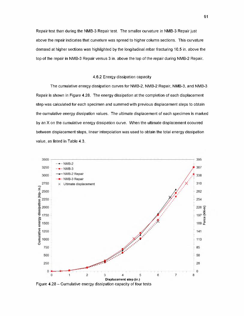
average displacement ductility of 5.95. NMB-2 Repair also dissipated 43% more cumulative

energy than NMB-2 at the ultimate displacement. NMB-3 Repair only achieved an average

displacement ductility of 3.66 due to a column longitudinal rebar fracturing prematurely during the

5-in. displacement step. The early rebar fracture during the NMB-3 Repair test is believed to be

due to welding of a threaded rod to the longitudinal bar. The embrittlement of the bar was shown

166

by the fracture surface of the bar being flat and the location of the fracture not matching any of

the other tests. From the results of NMB-2 Repair, it can be seen that the repair procedure is

capable of restoring all critical performance criteria of an earthquake damaged column.

Generalized STM modeling procedures have been developed to aid in the design of as-

built and repaired, column-to-footing, and column-to-pier cap assemblies. Two STM methods

have been used; the conventional STM and nonlinear STM. The conventional STM follows the

design guidelines within ACI 318, which does not take into account the degrading cyclic strength

of the model elements and predicts the ultimate load capacity of the assembly being modeled but

not the displacement. The nonlinear STM produces a force-displacement response envelope for

the assembly, using effective member strengths, which take into consideration the cyclic

degradation of the materials. When compared to the test results it can be seen that the

conventional STM can overpredict the ultimate load capacity of the assembly being modeled.

The conventional STM should be used to predict the monotonic strength of an assembly, and the

nonlinear STM should be used to predict the cyclic force-displacement envelope. This difference

in the models is best observed for LEN-2 Repair, which was tested both monotonically and

cyclically.

In addition to overpredicting the ultimate strength of half the specimens that were

modeled, the conventional STM vastly overpredicts the yield strength of the specimens, which is

defined as failure in the conventional STM. Yielding of rebar ties was the failure mode of both

repair models. This failure mode could lead a designer to believe the actual specimen would

have much more overstrength. However, this is not the case since the conventional STM

overpredicted the ultimate load capacity of LEN-2 Repair, which the model predicted as yielding

of the headed rebar ties. Both the overprediction of the ultimate load capacity and the

overprediction of the yield strength of the specimens show the unconservative nature of the

conventional STM. This should be expected when the conventional STM is used to model lateral

force resisting elements.

The nonlinear STM predicts the force-displacement response envelopes of the cyclically

damaged assemblies, which can be used to predict the ultimate load capacity, displacement

167

capacity, yield displacement, displacement ductility, and stiffness at varying displacements. The

nonlinear STM predicted the ultimate load capacities of the repaired column-to-footing and

repaired column-to-pier cap assemblies to be 82% and 92% of the tested capacities, respectively.

The nonlinear STM also predicted the ultimate displacement of the repaired column-to-footing

and repaired column-to-pier cap assemblies to be 88% and 84% of the tested capacities

respectively. When modeling the two as-built specimens, the nonlinear STM results, in terms of

ultimate load capacity, were slightly more conservative and underpredicted the ultimate load by

as much as 44%. However, the nonlinear STM seems to be a reasonable estimate of the force-

displacement characteristics for the as-built and repaired column-to footing and column-to-pier

cap assemblies.

6.1 Repair design recommendations

The design and procedure outlined in Chapter 3 was followed for NMB-2 Repair and

NMB-3 Repair, which successfully relocated the plastic hinge regions of the specimens.

Throughout the research process a few design improvements were recognized and should be

considered for future applications.

The thickness of the CFRP wrap should be larger than that calculated in Chapter 3 by an

appropriate margin of safety. The shear strength and confinement that the wrap provides is

paramount to the performance of the repair. To ensure proper performance from the CFRP wrap,

all available methods to mitigate transverse CFRP cracking should be taken. This includes

decreasing the cover of the headed rebar, which was 3 in. in this study. Also, additional means of

providing longitudinal strength to the CFRP wrap should be investigated. In previous tests that

have implemented this repair procedure on column-to-pier cap assemblies (34), the CFRP jacket

has ruptured. The rupturing of the CFRP jacket was thought to be due to brittle repair concrete,

high strength as-built concrete, high effective strength of the longitudinal rebar in the column,

minor damage during the as-built test above the height of the repair, and the early onset of

transverse CFRP cracking. This test demonstrated some of the factors that can rapidly increase

the demand on the jacket.

168

The amount of expansion in the repair concrete highly influences the behavior of the

repaired section. NMB-2 Repair was designed with Komponent as 13% of the cementitious

materials, whereas NMB-3 was designed with 41% Komponent. The 41% Komponent mix design

provided 14.6 times as much pre-tensioning of the CFRP jacket prior to testing than the 13%

Komponent mix design. The large amount of pre-tensioning provided in NMB-3 Repair did not

pose any problems, in fact it seemed to help the performance, but this was a short-term study

where the repaired column was tested 20 days after casting the repair concrete. It is believed

that the repair concrete used for NMB-3 Repair would have expanded much more with time,

decreasing the remaining strain capacity of the jacket. Further research should be conducted to

optimize the repair concrete mix design

6.2 Recommendations for further research

Further research should be conducted for the repair procedure as well as the STM

modeling procedures. More tests need to be conducted on precast GSS specimens of varying

geometries incorporating the repair, following the design recommendations provided in Section

6.1. It is also believed that the repair procedure would work well for column plastic hinges in

monolithic type bridge or building applications, but further research is needed to verify this.

Optimization of the repair concrete mix design would offer significant benefits to the repair

process. This includes the amount of expansion, the strength, and the workability of the concrete

for construction. Improvements to the CRFP wrap should be researched. This includes methods

to mitigate transverse cracking; including longitudinally oriented CFRP sheets, prefabricated

CFRP wraps, and decreasing headed rebar cover. The rapid application of the repair procedure

could be refined where bridge reopening times could be estimated. Rapid curing of the CFRP

wrap would need to be investigated. Also, repair concrete that has high early strength could be

used.

Many avenues exist for further research into STMs; some of the major topics are

mentioned here. An improved material force-displacement input for the longitudinal rebar in the

column should be investigated for the nonlinear STM. Due to the extremely large strain gradient

169

that eXists in the column longitudinal bars and their importance to the model a more accurate

input is needed. The current input used in this study was a bilinear curve that followed the steel

modulus up to the effective yield point and then followed a strain hardening ratio (s.h.r.) after the

effective yield, as recommended in previous research (18). The effective yield is the point at

which the eXtreme longitudinal rebar yields. However, since the tie represents five longitudinal

bars with highly varying distances to the neutral aXis, the stiffness beyond yield is dramatically

underpredicted by the s.h.r. An improvement to the force-displacement input would be to obtain it

from a sectional analysis, using a confined concrete model for the concrete in the column core

and an accurate tension steel model for the longitudinal bars in tension. This requires

incremental levels of concrete strain to be used, and the corresponding force in the longitudinal

rebar would need to be recorded. Once a satisfactory number of points were recorded from the

sectional analysis, the improved force-displacement input for the longitudinal rebar in the column

could be generated. This process could improve the input for any longitudinal tie that represents

multiple steel bars with varying moment arms.

Another aspect of the nonlinear STM that could use some refinement is the effective

strength of the CFRP confined concrete struts. This effective strength would need to be

determined from cyclic tests on CFRP confined concrete. The CFRP confined concrete model

used for the repair concrete struts and the allowable effective stress that was assigned to these

struts made the effective strength less than the unconfined concrete strength. This is a highly

conservative approach. Although the CFRP confined concrete struts did not control any of the

loads in this study, it still needs to be refined.

The last research recommendation for the nonlinear STM would be to refine the plastic

hinge length of the precast GSS specimens. This improvement would help to better predict the

last point of the nonlinear STM output for the as-built specimens. Also, including concrete ties in

the model could improve results by increasing the initial stiffness.

REFERENCES

(1) California Department of Transportation. Seismic design criteria; Division of EngineeringServices, Sacramento, CA. 2010.

(2) Ameli, M.J. Seismic Design of Grouted Splice Sleeve Connections for Bridge Piers used inAccelerated Bridge Construction. Ph.D. Dissertation, University of Utah, Salt Lake City, UT, to be submitted for publication (2015).

(3) Haber, Z.; Saiidi, M.; Sanders, D. Precast Column-Footing Connections for AcceleratedBridge Construction in Seismic Zones; Final Report No. CA13-2290; Nevada, 2013.

(4) Belleri A.; Riva, P. Seismic Performance and Retrofit of Precast Concrete Grouted SleeveConnections. PCI J. 2012, 57, 97-109.

(5) American Concrete Institute. ACI 318-11 Building Code Requirements for Structural Concrete;Farmington Hills, MI, 2011.

(6) Seible, F.; Priestley, M.J.; Hegemier, G. Seismic Retrofit of RC Columns with ContinuousCarbon Fiber Jackets. J. Compos. Constr. 1997, 1, 52-62.

(7) Pantelides, C.P.; Gergely, I.; Reaveley, L.D.; Volnyy, V.A. Retrofit of R/C Bridge Pier with CCFRP Advanced Composites. J. Struct. Eng., 1999, 125, 1094-1099.

(8) Chai, Y.; Priestley, M.J.; Seible, F. Seismic Retrofit of Circular Bridge Columns for EnhancedFlexural Performance. ACI Structural J. 1991, 88, 572-584.

(9) Lehman, D.; Gookin, S.; Nacamuli, A.; Moehle, J. Repair of Earthquake-Damaged BridgeColumns. ACI Structural J. 2001, 98, 233-242.

(10) Hose, Y.D; Seible, F; Priestley, M.J. Strategic Relocation of Plastic Hinges in BridgeColumns, SSPR 97-05.

(11) Rutledge, S.; Kowalsky, M.;Seracino, R.; Nau, N. Repair of Damaged Circular ReinforcedConcrete Columns by Plastic Hinge Relocation, Proceedings of the 15 WCEE, Lisbo, 2012.

(12) American Association of State Highway and Transportation Officials (AASHTO). AASHTOLRFD Bridge Design Specifications. AASHTO: Washington, DC 2012.

(13) Saenz N.; Pantelides, C.P.; Reaveley, L.D. Strut-and-tie model for shear friction of concretewith fiber-reinforced polymer composites. ACI Structural J. 2004, 101, 863-871.

(14) Park S.; Aboutaha R.S. Strut-and-tie method for CFRP strengthened deep beams. J.Structural Eng. 2009, 135, 632-643.

171

(15) Hong, S.G.; Chun, S.C.; Lee, S.H.; Oh, B. Strut and Tie Model for Development of HeadedBars in Exterior Beam Column Joint. ACI Structural J. 2007, 104, 590-600.

(16) To, N.H.T.; Ingham, J.M.; Sriharan, S. Strut-and-tie computer modelling of reinforcedconcrete bridge joint systems. J. Earthquake Eng. 2003, 7, 463-493.

(17) To, N.H.T.; Ingham, J.M.; Sriharan, S. Strut-and-tie computer modelling of reinforcedconcrete bridge portal frames. Bulletin of the New Zealand Society for Earthquake Eng. 2002,165-189.

(18) To, N.H.T.; Ingham, J.M.; Sriharan, S. Monotonic nonlinear strut-and-tie computer models.Bulletin of the New Zealand Society for Earthquake Eng. 2001, 169-190.

(19) Park, H.; Eom, T. Truss model for nonlinear analysis of RC members subject to cyclicloading. J. Structural Eng. 2007, 133, 1351-1363.

(20) To, N.H.T.; Sriharan, S.; Ingham, J.M. Strut-and-tie nonlinear cyclic analysis of concreteframes. J. Structural Eng. 2009, 135, 1259-1268.

(21) American Association of State Highway and Transportation Officials (AASHTO). AASHTOGuide Specifications for LRFD Seismic Bridge Design. AASHTO: Washington, DC 2011.

(22) American Concrete Institute. ACI 374.2-13 Guide for Testing Reinforced Concrete StructuralElements under Slowly Applied Simulated Seismic Loads; Farmington Hills, MI, 2013.

(23) Hilti Corporation. Technical application document: Hilti HIT-RE 500-SD; Champs sur Marne,France, 2010.

(24) Mortazavi, A.A.; Pilakoutas, K.; Sang Son, K. RC column strengthening by lateral pre­tensioning of FRP. Constr. and Build. Mater. 2003, 17, 491-497.

(25) Zihan, Y.; Pantelides, C.P.; Reaveley L.D. Fiber-reinforced polymer jacketed and shape-modified compression members: I-Experimental behavior. ACI Structural J. 2006, 103, 885-893.

(26) Priestley, M.J.N.; Seible, F. Design of seismic retrofit measures for concrete and masonrystructures. Constr. and Building Materials 1995, 5, 365-377.

(27) Pantelides, C.P.; Moran, D.A. Design of FRP jackets for plastic hinge confinement of RCcolumns. J. Compos. Constr. 2013, 17, 881-898.

(28) ASTM Standard A370, 2012, “Methods for Testing Steel Reinforcing Bars,” ASTMInternational, West Conshocken, PA, 2012, DOI 10.1520/C0109_C0109M, www.astm.org.

(29) ASTM Standard D3039, 2008, “Standard Test Method for Tensile Properties of PolymerMatrix Composite Materials,” ASTM International, West Conshocken, PA, 2008, DOI 10.1520/D3039_D3039M-08, www.astm.org.

(30) ASTM Standard C39, 2012, “Standard Test Method for Compressive Strength of CylindricalConcrete Specimens,” ASTM International, West Conshocken, PA, 2012, DOI 10.1520/C0039_C0039M-12A, www.astm.org

172

(31) ASTM Standard A109, 2012, “Standard Test Method for Compressive Strength of HydraulicCement Mortars (Using 2-in. Cube Specimens,” ASTM International, West Conshocken, PA, 2012, DOI 10.1520/A0307-12, www.astm.org.

(32) CTS Cement Manufacturing Corporation. KSC concrete technical guide; Cypress, CA, 2013.

(33) American Concrete Institute. ACI 440.2R-08 Guide for the Design and Construction ofExternally Bonded FRP Systems for Strengthening Concrete Structures; Farmington Hills, MI, 2008.

(34) Parks, J.E. Seismic rehabilitation of column to pier cap accelerated bridge constructionconnections and acoustic emission monitoring assessment. Masters Thesis, University of Utah, Salt Lake City, Utah, 2012

(35) Moran, D.; Pantelides, C. Elliptical and Circular FRP-Confined Concrete Sections: A Mohr-Coulomb Analytical Model. Int. J. Solids and Struct. 2012, 49, 881-898.

(36) Xiao, Y.; Priestley, M.J.; Seible, F. Seismic Assessment and Retrofit of Bridge ColumnFooting. ACI Structural J. 1996, 93, 79-94.

(37) Collins, M.P.; Mitchell, D.; Adebar, P.; Vecchio, F.J. A General Shear Design Method. ACIStructural J. 1996, 93, 36-45.

(38) Priestley, M.J.N.; Seible, F.; Calvi, G.M. Seismic Design and Retrofit of Bridges; John Wiley& Sons, Inc.: New York, 1996.

(39) Mander, J.B.; Priestley, M.J.N.; Park, R. Theoretical Stress-Strain Model for ConfinedConcrete. J. Structural Division 1988, 114, 1804-1826.

(40) Lam, L.; Teng, J.G. Design-Oriented Stress-Strain Model for FRP-Confined Concrete.Constr. and Build. Mater. 2003, 17, 471-489.

(41) Sika Corporation. Product data sheet: SikaWrap Hex 103C; Lyndhurst, NJ, 2011


Recommended