Presented By Kenneth Davis Potential of the Spectral Element Method in Flow Simulations of Aerospace Systems K.E. Davis and B.C. Houchens Thermal & Fluids Analysis Workshop TFAWS 2010 August 16-20, 2010 Houston, TX TFAWS Paper Session
Transcript
Presented By
Kenneth Davis
Potential of the Spectral Element
Method in Flow Simulations of
Aerospace Systems
K.E. Davis and B.C. Houchens
Thermal & Fluids Analysis Workshop
TFAWS 2010
August 16-20, 2010
Houston, TX
TFAWS Paper Session
TFAWS 2010 – August 16-20, 2010 2
Overview
• Code development
– Utilizes the spectral element method to solve incompressible
fluid flow and heat transfer equations
– Written from scratch
– Can handle complex geometries
– Arbitrary application of boundary conditions
– Several typical boundary conditions
• Advantages over commercial software
– Total control
– Application of “unusual” boundary conditions
– More accuracy
– More cost-effective
TFAWS 2010 – August 16-20, 2010 3
Why Use Spectral Elements?
• Accuracy
– Can refine in p as well as h to improve accuracy
– Finite elements and finite volumes are usually limited to h
refinement
– p refinement yields better results than h refinement
• No need for stabilization
– Finite elements generally use elements (such as linear-linear)
that require stabilization
– Spectral elements are stable when using the PN – PN-2 grids
• Can handle complex geometries
– Finite difference methods are limited to simple domains
TFAWS 2010 – August 16-20, 2010 4
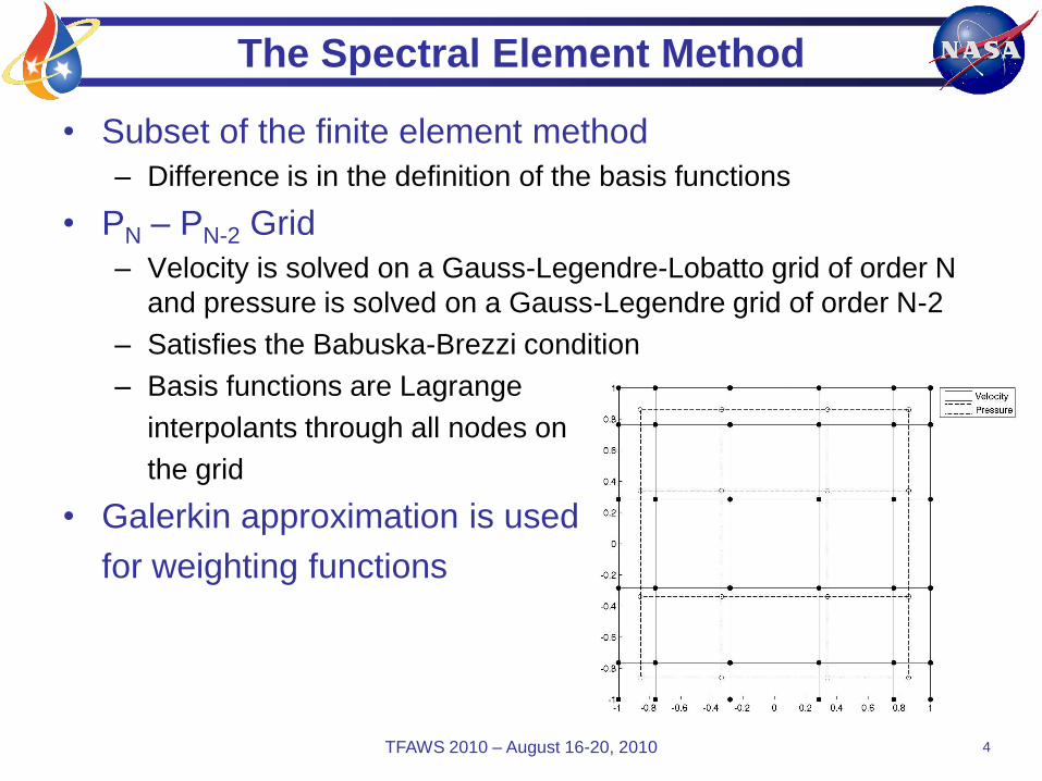
The Spectral Element Method
• Subset of the finite element method
– Difference is in the definition of the basis functions
• PN – PN-2 Grid
– Velocity is solved on a Gauss-Legendre-Lobatto grid of order N
and pressure is solved on a Gauss-Legendre grid of order N-2
– Satisfies the Babuska-Brezzi condition
– Basis functions are Lagrange
interpolants through all nodes on
the grid
• Galerkin approximation is used
for weighting functions
TFAWS 2010 – August 16-20, 2010 5
The Spectral Element Method
• Discretize the domain
– First using meshing software such as Gambit
– Then build the spectral mesh on each element
• Approximate solution
–
• Procedure
– Multiply by test function
– Integrate over each element
– Scatter to global matrices
– Newton-Raphson iterations
• Solve the resulting linear system using GMRES or BiCGStab
– Write data
Solver Structure
TFAWS 2010 – August 16-20, 2010 6
Build Geometry
with CAD
software
Mesh Geometry
with Gambit
Input File
Read Input
Build Matrices
Assemble Linear
System
Solve Linear
System
End
Build Spectral
Mesh
Converged?
Transient?More Time
Steps?
No
No
Yes
No
Yes
Yes
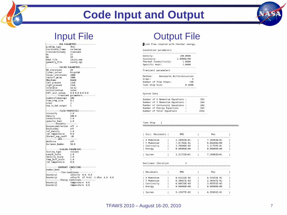
Code Input and Output
TFAWS 2010 – August 16-20, 2010 7
Input File Output File
TFAWS 2010 – August 16-20, 2010 8
Current Code Capabilities
• General geometries are represented exactly (2D only)
– Code reads IGES files and stores geometry parameters for each
curve
– Must find where mesh and geometry coincide
– Allows for exact computation of Jacobian
• Boundary conditions can be applied to any boundary
– Fluid boundary conditions
• Velocity components
• Stress components
• Mixed velocity/stress components
– Thermal boundary conditions
• Temperature
• Heat flux
– All boundary conditions can vary with space
– Velocity and temperature can vary with time
TFAWS 2010 – August 16-20, 2010 9
Current Code Capabilities
• Initial conditions can vary with space
• Cartesian – 2D and 3D, Cylindrical – 2D only
– 2D cylindrical coordinates refers to axisymmetric flows, meaning
the coordinates are r and z
– Currently extending the 3D code to solve in cylindrical
coordinates
• High-order transient solutions
– Attempted Adams-Moulton method, but it was unstable
– Now use backwards differentiation up to 6th order
• Buoyancy
– Boussinesq approximation can be applied
•
TFAWS 2010 – August 16-20, 2010 10
Pre-processing Matlab GUI
• Pre-processor writes input file for code
• Provides a simple interface for users unfamiliar with the
code and its input file
TFAWS 2010 – August 16-20, 2010 11
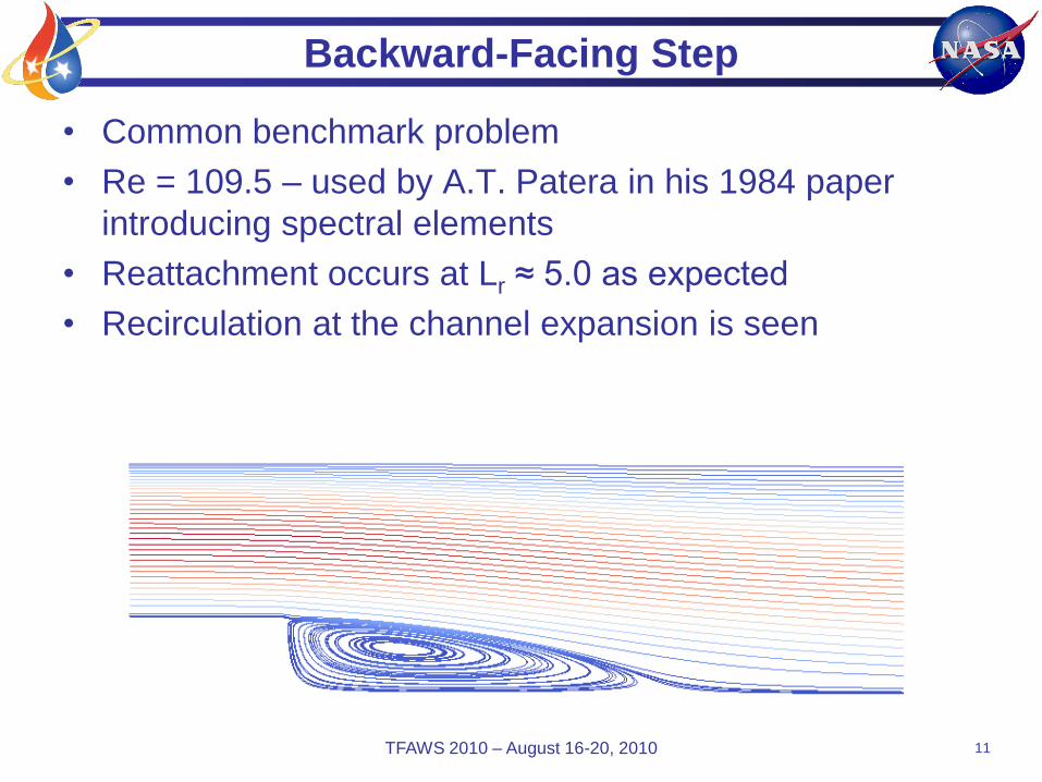
Backward-Facing Step
• Common benchmark problem
• Re = 109.5 – used by A.T. Patera in his 1984 paper
introducing spectral elements
• Reattachment occurs at Lr ≈ 5.0 as expected
• Recirculation at the channel expansion is seen
TFAWS 2010 – August 16-20, 2010 12
Lid Driven Cavity Flow
• Re = 400
• Top side has dimensionless velocity of 1 to left; all other
sides are at rest
• Recirculations qualitatively accurate and the u velocity
on the vertical centerline agrees well with previous
results
TFAWS 2010 – August 16-20, 2010 13
Kovasznay Flow
• Flow behind a two dimensional
grid
• Exact solution given by L.I.G.
Kovasznay in 1948
–
–
–
–
• Re = 40 for this simulation
• Dirichlet boundary conditions
were applied
• Obtained a solution where the L2 norm of the error in
velocity is less than 10-10
TFAWS 2010 – August 16-20, 2010 14
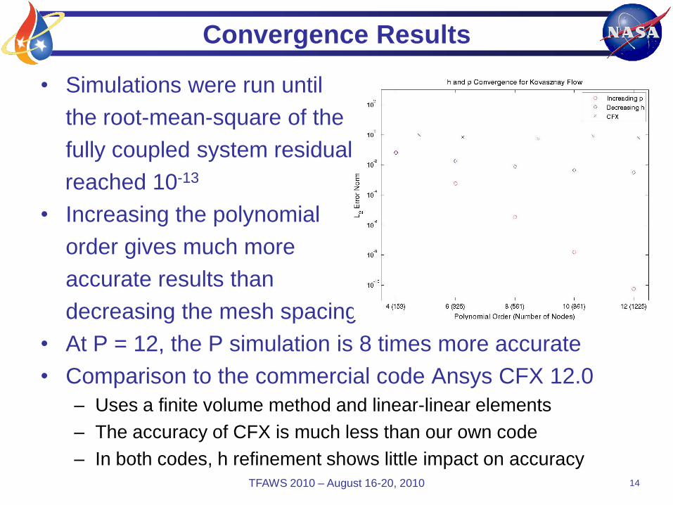
Convergence Results
• Simulations were run until
the root-mean-square of the
fully coupled system residual
reached 10-13
• Increasing the polynomial
order gives much more
accurate results than
decreasing the mesh spacing
• At P = 12, the P simulation is 8 times more accurate
• Comparison to the commercial code Ansys CFX 12.0
– Uses a finite volume method and linear-linear elements
– The accuracy of CFX is much less than our own code
– In both codes, h refinement shows little impact on accuracy
TFAWS 2010 – August 16-20, 2010 15
Current Activity
• Linear solver
– Currently solve fully coupled system using ILU(0) preconditioned
Krylov subspace methods
– Implemented multigrid, but not to satisfaction
• Preconditioning
– Currently use ILU(0), but may need something more