Chapter 6
POTENTIAL THEORY AND HEAT CONDUCTION
DIRICHLET’S PROBLEM
© M. Ragheb
9/19/2013
6.1 INTRODUCTION
The solution of the Dirichlet problem is one of the easiest approaches to grasp
using Monte Carlo methodologies. The Dirichlet problem consists in finding a function u
that is defined, continuous, and differentiable over a closed domain D with boundary C
and satisfying Laplace’s Equation:
,
,02
Confu
Donu
(1)
where: f is some prescribed function, and 2 is the Laplacian operator.
This problem appears in heat transport, fluid flow, plasma simulations and
multiple other potential problems applications.
One could deduce a Monte Carlo solution by covering the domain D by a cubic
mesh, and replacing the Laplacian operator by its finite difference equivalent. A random
walk or Pólya walk that is started from an inner point and moving to the boundary,
determines the solution at the starting point.
One can visualize the random walk as a walk undertaken by a drunken or
inebriated person walking in a city, walking at intersections north, south, east or west
with equal probability, his walk stopping when he reaches the city wall or boundary.
6.2 DIRICHLET’S PROBLEM, LAPLACE’S EQUATION
We consider the Monte Carlo simulation of steady state heat conduction in an
isotropic and homogeneous non-energy generating solid. The objective is to find a
solution to a multidimensional function u(x, y) satisfying the two-dimensional Partial
Differential Equation (PDE):
,0),(),(
),(2
2
2
22 Don
y
yxu
x
yxuyxu
(2)
with a boundary condition:
.),( Conyxfu (3)
where f(x, y) is a prescribed function.
In one-dimensional problems one can replace the 2 operator by its finite
difference approximation:
02
2
x
x
u
x
u
dx
du
dx
d
dx
ud (4)
From which, from Fig. 1:
02
,1,,,1
x
uuuu jijijiji
Consequently:
02
2
,,1,1
x
uuu jijiji
Let us denote:
hx ,
thus:
02
2
,1,1
2
2
h
uuu
dx
ud jijiji. (5)
In two-dimensional problems we can similarly write for hyx :
2 2
1, 1, , 1 , 1
2 2 2
4( , ) ( , )0
i j i j i j i j i ju u u u uu x y u x y
x y h
(6)
Solving for ui,j, we get:
4
1,1,,1,1
,
jijijiji
ji
uuuuu (7)
This implies that each internal point is an average over the surrounding mesh
points including the boundary points. The averaging process is a characteristic of
potential problems in general. This implies a Pólia walk or random walk with equal
probabilities of moving from a mesh point to its four immediate neighbors in two
dimensions, and to its six immediate neighbors in three dimensions.
We assume for simplicity that the boundary C surrounding the domain D lies on
the mesh as shown in Fig. 1.
Figure 1. Solution of the Laplace’s Equation using a random walk on a two-dimensional
grid.
Figure 2. Probability density function (pdf) and cumulative distribution function (cdf) for
sampling the direction θ in a random walk.
6.3 RANDOM WALK PROCEDURE
A pseudo particle is started from an interior point P of the domain D and we
generate a random walk where the particle has equal probability of stepping to one of
four neighboring points randomly.
The discrete probability density function and the cumulative distribution function
are shown as a function of the angle θ in Fig. 2. As random numbers are generated over
the interval [0,1], they are compared to the possibly tabulated value of the cumulative
distribution function to sample a direction to the right, left, up or down, or alternatively,
north, East South or West.
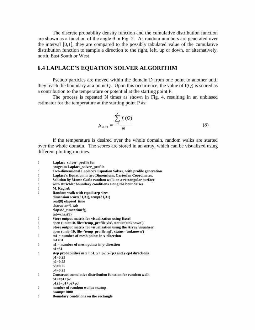
6.4 LAPLACE’S EQUATION SOLVER ALGORITHM
Pseudo particles are moved within the domain D from one point to another until
they reach the boundary at a point Q. Upon this occurrence, the value of f(Q) is scored as
a contribution to the temperature or potential at the starting point P.
The process is repeated N times as shown in Fig. 4, resulting in an unbiased
estimator for the temperature at the starting point P as:
N
QfN
i
i
Pu
1
)(
)(
(8)
If the temperature is desired over the whole domain, random walks are started
over the whole domain. The scores are stored in an array, which can be visualized using
different plotting routines.
! Laplace_solver_profile for
program Laplace_solver_profile
! Two-dimensional Laplace's Equation Solver, with profile generation
! Laplace's Equation in two Dimensions, Cartesian Coordinates.
! Solution by Monte Carlo random walk on a rectangular surface
! with Dirichlet boundary conditions along the boundaries
! M. Ragheb
! Random walk with equal step sizes
dimension score(31,31), temp(31,31)
real(8) elapsed_time
character*1 tab
elapsed_time=timef()
tab=char(9)
! Store output matrix for visualization using Excel
! open (unit=10, file='temp_profile.xls', status='unknown')
! Store output matrix for visualization using the Array visualizer
open (unit=10, file='temp_profile.agl', status='unknown')
! m1 = number of mesh points in x-direction
m1=31
! n1 = number of mesh points in y-direction
n1=31
! step probabilities in x+:p1, y+:p2, x-:p3 and y-:p4 directions
p1=0.25
p2=0.25
p3=0.25
p4=0.25
! Construct cumulative distribution function for random walk
p12=p1+p2
p123=p1+p2+p3
! number of random walks: nsamp
nsamp=1000
! Boundary conditions on the rectangle
! left t1=t(0,y), bottom t2=t(x,0), right t3=t(m1,y), upper t4=t(x,n1)
t1=100.
t2=0.
t3=100.
t4=0.
! Coordinates indices of point at which solution is estimated
! m: i0=x/dx, n: j0=y/dy
do 30 m=2,30,1
do 30 n=2,30,1
! m=11
! n=11
! Start random walk here
! Initialize counters
! History counter
ncount=0
! Score counter
score(m,n)=0.0
! Initiate random walk
99 i=m
j=n
999 call random(r)
! Sample cumulative distribution function for random walk
! Move one step to the right
if (r le.p1) then
i=i+1
goto 11
! Move one step up
else if (r le.p12) then
j=j+1
goto 11
! Move one step left
else if (r le.p123) then
i=i-1
goto 11
else
! Move one step down
j=j-1
goto 11
end if
! Check for random walk reaching boundary
! Check whether lower boundary is reached
11 if (j.eq.1) then
score(m,n) = score(m,n) + t2
goto 88
! Check whether right boundary is reached
else if (i.eq m1) then
score(m,n) = score(m,n) + t3
goto 88
! Check whether upper boundary is reached
else if (j.eq n1) then
score(m,n) = score(m,n) + t4
goto 88
! Check whether left boundary is reached
else if (i.eq.1) then
score(m,n) = score(m,n) + t1
! write(*,*) score
goto 88
else
goto 999
end if
! Increment history counter
88 ncount=ncount+1
! Check for total number of histories
if (ncount lt nsamp) then
goto 99
else
goto 77
end if
! Calculate solution at points of interest
77 xcount=ncount
temp(m,n)=score(m,n)/xcount
! write(10,*) temp(m,n)
! write(*,*) score
! write(*,*) xcount
! Print results
30 continue
write(*,*)'number of random walks=',nsamp
! write(*,*)'coordinate of point at which temperature is calculated',m,n
! write(*,*)'calculated temperature=',temp
write(*,300) temp
! Boundary values
do 40 i=1,31
do 40 j=1,31
! bottom boundary
temp(i,1)=0.0
! top boundary
temp(i,31)=0.0
! left boundary
temp(1,j)=100.0
! right boundary
temp(31,j)=100.0
40 continue
do 20 n=1,31
write(10,300) (temp(m,n),tab, m=1,31)
20 continue
300 format(31(e14.8,a1))
elapsed_time=timef()
write(*,*) elapsed_time
stop
end
Figure 3. Procedure for the Monte Carlo solution of Laplace’s Equation Dirichlet’s
problem temperature profile using a random walk approach.
For a boundary condition of f(Q) = 100 degrees on one boundary, and f(Q) = 0 on
the three other boundaries, the solution u(x,y) is plotted using the plotting feature in the
Excel program in Fig. 4.
For a boundary condition of f(Q) = 100 degrees on two opposing boundaries , and
f(Q) = 0, on the other two opposing boundaries, the solution u(x,y) is plotted using the
Array Visualizer plotting routine in Figs. 5 and 6.
Figures 7 and 8 show the solution for a boundary condition of f(Q) = 100 degrees
on one boundary, f(Q) = 50 degrees on the adjoining boundary and f(Q) = 0 on the other
two boundaries. The solution u(x, y) is plotted using the Array Visualizer plotting
routine for a number of 1,000 particles started on a 31x31 nodes domain. The execution
time on a desktop computer was about 17 seconds.
6.4 FLOATING POINT RANDOM WALK IN HEAT CONDUCTION
Consider S(P) to be the largest sphere in three dimensions or circle in two
dimensions centered at P that does not go outside the domain D. From potential theory,
the solution at P, u(P) is equal to the average value of u over the surface of S(P). One can
take a sequence of points:
P = P0, P1, P2, … , Pm+1
where Pm+1 is a random point on the surface of S(Pm), until a point is reached that is
sufficiently close to the boundary C. If Q is now the nearest point actually on C, f(Q) is
taken for the estimator of u(P).
This approach can be generalized to be a shape other than a sphere or a circle,
provided one knows the Green’s function of that surface. The methodology economizes
the number of random walk steps by reaching the boundary of the sphere in a single
jump, instead of by way of the individual steps on the equivalent lattice.
Figure 4. Monte Carlo solution of Laplace’s Equation Dirichlet’s problem temperature
profile.
y
Temp [degrees C]
x
Figure 5. Monte Carlo solution of Laplace Equation Dirichlet’s problem with temperature
profile visualization, Height Plot.
Figure 6. Monte Carlo solution of Laplace Equation Dirichlet’s problem temperature
profile visualization, Image Map.
Figure 7. Monte Carlo solution of Laplace’s Equation Dirichlet’s problem temperature
profile visualization, Height Plot.
Figure 8. Monte Carlo solution of Laplace’s Equation Dirichlet’s problem temperature
profile visualization, Image Map.
If the exact solution for a preselected geometry is known one can also use a
floating random walk and avoid the use of the mesh points. The simplest solution for a
finite and homogeneous domain is the temperature at the center of cylinders and spheres.
This exact solution for the temperature at a point (x, y) at the center of a homogeneous
cylinder is given by:
1
0
20,2
).,(),(
druyxu (9)
where:
2
ddF is the normalized probability density function for the distribution of the
azimuthal angle φ, and u(r,φ) is the temperature at the boundary of a circle of radius r.
The probability density function (pdf) dF suggests that a random walker at (x, y),
the center of a circle or sphere,, has equal probability of getting to any point on the
circumference of the circle or sphere of radius r.
One thus considers a circle or a sphere surrounding a point (x0,y0) at which a
random walker has arrived after several steps, and which just meets the nearest portion of
the boundary.
The cumulative distribution function (cdf) for φ is sampled with the aid of a
random number ρ:
]1,0[,22
)(0
d
(10)
leading to a sampled angle:
2 (11)
The new position of the random walker will be:
sin
cos
0
0
ryy
rxx
new
new
(12)
The process is repeated until the random walk is terminated through absorption at the
boundary. The walk does not proceed along grid points and lines, and the direction and
step size are variable.
In three dimensions, the temperature distribution at the center of a sphere is given
by:
1
0
1
0
)sin2
1()
2(),,(),,(
d
druzyxu (13)
The azimuthal angle is sampled from:
]1,0[,22
)( 11
0
d
(14)
Figure 9. Two-dimensional geometry for a floating random walk.
The polar angle is sampled from:
2
0
0
)cos1(2
1
|cos2
1
sin2
1)(
d
(15)
Inverting Eqn. 15 yields:
221cos ,
)21(cos 2
1 (16)
The coordinates of the pseudo-particles at the new point will be:
cos
sinsin
cossin
0
0
0
ryz
rzy
rxx
new
new
new
(17)
6. 5 DISCUSSION
The Dirichlet problem can be reduced to the form of a linear system of equations
to be solved itself by Monte Carlo:
xASx (18)
where the order of A is equal to the number of mesh points in D. The matrix A has four
elements equal to ¼ in each row corresponding to an interior point D, all other points
being zero.
The previous analysis constitutes an “adjoint” solution moving from the detector
location to the source. An alternative solution could adopt the “forward” solution
approach, starting from the source at the boundary to the interior detector points within
the boundary.
The Monte Carlo method has been applied to conductive and radiative heat
transport. Its application to convective heat transport has been minimal despite the fact
that energy transport in turbulent flows depends primarily on random processes.
Monte Carlo simulations can be used a wide range of conduction problems:
1. Steady state conduction,
2. Transient conduction,
3. Various geometrical configurations,
4. Different boundary conditions including radiative and convective heat transport
with volumetric sources.
5. Anisotropic and nonhomogeneous media.
The approach is useful in these areas of application whenever:
1. There is no other analytical or numerical solution to the problem,
2. Checking the validity of new stochastic, numerical or analytical methods,
3. Developing models for complex processes, and checking them against
experimental values,
4. Monte Carlo can offer in some cases a faster approach than other methods such as
finite differences, particularly in multidimensional problems.
EXERCISES
1. To account for anisotropic media problems, modify the conductivity of a medium
to encourage heat flow in one direction, then compare your result to the isotropic case.
This would entail modifying the probabilities of scattering in the random walk, while still
maintaining a valid probability profile.
2. Modify the Laplace’s solver procedure to solve the Laplace’s Equation Dirichlet’s
Problem in three dimensions, using a consistent set of boundary conditions. Use the
Array Visualizer to show the temperature distribution in plane slices.
3. Solve the Dirichlet’s problem with a mixed type of boundary conditions defined
on segments of the same boundary.
4. Modify the random walk procedure to make the conductivity spacially-dependent
in an anisotropic medium. Start the formulation using the Laplace’s equation.
5. Solve the Laplace equation analytically for a temperature of 100 degrees on the
right boundary, zero degrees on the left boundary, and reflective boundary conditions on
the top and bottom boundaries. Compare the analytical result to the Monte Carlo
simulation result.
6. Study the effect of the increase of the node points in the random walk procedure,
and the effect of the increase of the number of histories, on the execution time of the
algorithm.
7. Modify the algorithm from a Cartesian mesh to a triangular mesh, which would
allow for a better treatment of curved surfaces. Use the triangular mesh to approximate a
complex geometry such as an ellipsoid.