POVERTY DYNAMICS AND HOUSEHOLD RESPONSE: DISASTER …

The Pennsylvania State University

The Graduate School

College of Agricultural Sciences

POVERTY DYNAMICS AND HOUSEHOLD RESPONSE: DISASTER SHOCKS IN RURAL BANGLADESH

A Thesis in

Agricultural, Environmental and Regional Economics and Demography

by

Anuja Jayaraman

© 2006 Anuja Jayaraman

Submitted in Partial Fulfillment of the Requirements

for the Degree of

Doctor of Philosophy

August 2006

The thesis of Anuja Jayaraman was received and approved* by the following Jill. L. Findeis Professor of Agricultural, Environmental and Regional Economics and Demography Thesis Advisor Chair of Committee Carolyn E. Sachs Professor of Rural Sociology and Women’s Studies Gretchen T. Cornwell Research Associate and Assistant Professor of Rural Sociology and Demography Bee-Yan Roberts Professor of Economics Stephen M. Smith Professor of Agricultural and Regional Economics Committee Member and Head of Department of Agricultural Economics and Rural Sociology * Signatures are on file in the Graduate School.

Abstract

South Asia has the largest concentration of the world’s poor, with over half a

billion people surviving on less than a dollar a day. One of the Millennium Development

Goals (MDG) aims to halve the proportion of the world’s people whose income is less

than one dollar a day and the proportion of people who suffer from hunger by the year

2015. The success of poverty alleviation programs in South Asia is critical if this MDG

is to be met. Within South Asia, Bangladesh has the highest incidence of poverty and

only India and China have larger numbers of poor people. It is estimated that nearly half

of Bangladesh’s population of 135 million people live below the poverty line. The

Human Poverty Index reported by the Human Development Report places Bangladesh at

the 86th position among 103 developing countries. Apart from high poverty levels and

low gender empowerment rates, the country also faces yearly natural disasters in the form

of floods. In this dissertation, we first analyze issues relating to chronic and transient

poverty following a major catastrophic event using a short panel of household data from

Bangladesh. Bangladesh experienced the largest floods of the century in 1998. Increase

in private borrowing was one of the medium-term impacts of the floods. The

International Food Policy Research Institute’s Food Management and Research Support

Project (IFPRI-FMRSP) household survey of rural Bangladesh for the years 1998-99 is

used for the analysis. The dissertation attempts to identify the characteristics that

distinguish between those who are able to eventually escape poverty following the flood

(the transient poor) versus those unable to leave poverty (chronic poor). The study uses

cost-of-basic-needs (CBN) poverty lines calculated by the World Bank for Bangladesh

for the year 2000. We use multinomial logit models to asses the determinants of chronic

iii

and transient poverty, comparing them to Bangladeshi households that were never poor.

We also use Censored Quantile Regression models to identify the correlates of each kind

of poverty.

We find that household size, dependency ratio, number of working members, land

ownership, location, social assistance and education characterize the chronically poor.

Ownership of physical and human capital make households less likely to be chronically

poor. Larger household size and dependents in the household push families towards

chronic poverty. Increase in number of working members in the family bring in more

income and reduce the chances of households being chronically poor. Given that

Bangladesh is an agrarian society and faces yearly floods, it is not surprising that

households with heads employed in the trade and self-employment sectors are less likely

to be chronically poor compared to those in the agricultural sector. Long term

investments in human and physical assets clearly help households out of chronic poverty.

Apart from household size, dependency ratio, number of working members, and land

ownership, the transient poor are characterized by their access to credit. Credit access

and remittances explain transient poverty better. Our models are not able to characterize

the transient poor as well as the chronically poor.

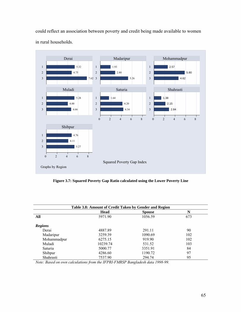
After having studied the poor and their characteristics, we seek to study how

individuals interact and operate within a family or household. We asses intra-household

dynamics (e.g., variations in household bargaining behaviors) with a focus on the

household’s expenditure patterns. Receipt of credit is taken as the measure of bargaining

between the head and the spouse. Food and non-food share equations were individually

estimated using random effect OLS and Tobit models to test if participation in credit

iv

markets influences food and non-food expenditure shares. Endogeneity corrections were

incorporated whenever tests indicated an endogenous relationship between total

household consumption and a particular expenditure share. 2SLS models and

simultaneous Tobit models were used to correct for endogeneity between the expenditure

shares and total expenditure. Our results indicate that more men compared to women

participate in the credit market. As is typical of any rural-developing economy,

household expenditure share is highest for food. Amount borrowed by the household

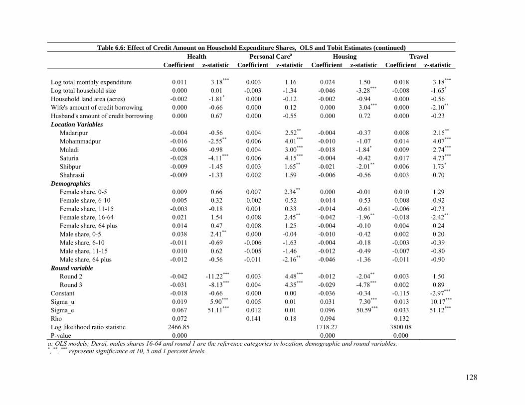
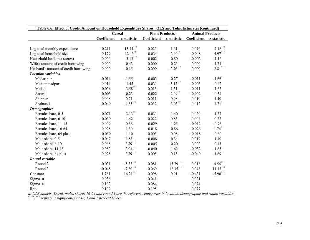
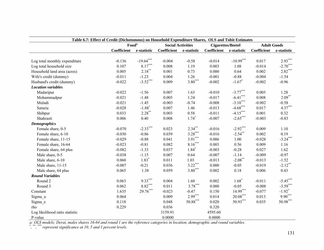
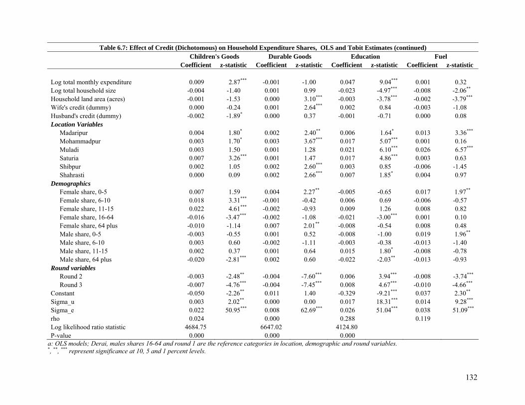
head has effects on food expenditure, adult goods and education expenditure. Amount of

credit taken by the household head negatively affects food expenditure and positively

affects share spent on adult goods. The negative effect on food expenditure has policy

implications related to nutritional intake of children in the household. Women and girls

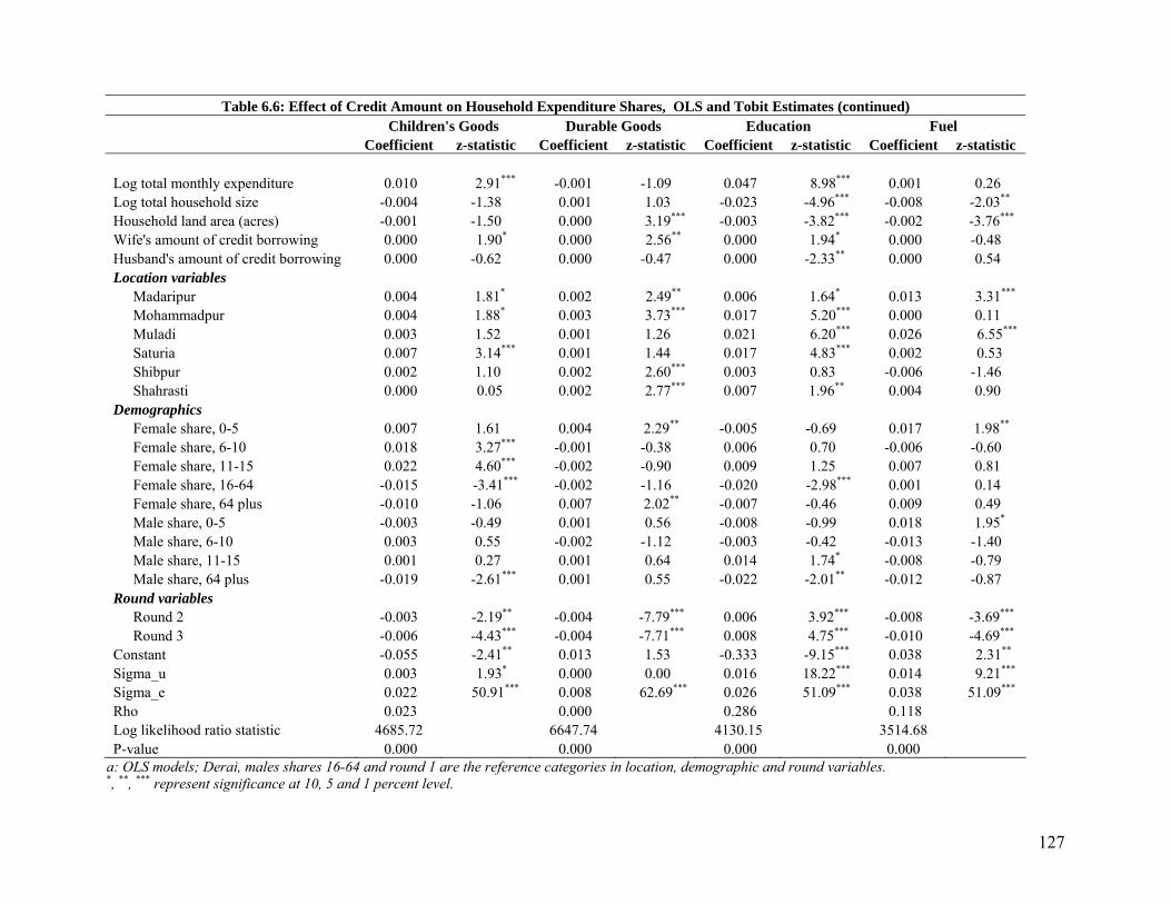
in the household may also suffer from resultant nutritional deficiencies. Women’s use of

credit has a positive impact on expenditure on children’s goods, durable goods, education

and housing. Results show that resources in the hands of women have implications for

improvement in child outcomes, especially educational outcomes. The positive and

significant impact of spouse’s credit on housing share indicates that resources in the

hands of women also go towards improvement in household and related outcomes. We

also find that households are more likely to spend in round 2 and round 3 than in round 1

on food, education and personal care and more likely to spend on adult goods, children’s

goods, durable goods, fuel, health and housing in round 1 than in round 2 or 3.

v

Table of Contents List of Tables viii List of Figures ix Acknowledgements x 1 Chapter 1: Research Problem 11.1 Introduction 11.2 Poverty and Vulnerability to Shocks 31.3 Shocks in Bangladesh 71.4 Poverty in Bangladesh 81.5 Consumption Smoothing 111.6 Gender and Poverty 131.7 Study Objectives 141.8 Organization of the Dissertation 16 2 Chapter 2: Literature Review and Theoretical Framework 172.1 Introduction 172.2 Poverty Dynamics 182.2.1 Definition of Chronic and Transient Poverty 192.2.2 Measuring Chronic and Transient Poverty 202.2.3 Empirical Studies 222.2.4 Characteristics of the Chronically Poor 252.2.5 Characteristics of the Transient Poor 262.3 Intrahousehold Resource Allocation Models 272.3.1 Unitary Household Model 272.3.2 Agricultural Household Models 302.3.3 Collective Models 332.3.4 Cooperative Model 332.3.5 Cooperative Bargaining Models 362.3.6 Non-Cooperative Model 42 3 Chapter 3: Data and Descriptions 443.1 Country of Study: Bangladesh 443.2 Data Characteristics 503.2.1 Sampling Procedure 533.3 Research Trip to Bangladesh, February 2005 543.4 Data Description 573.4.1 Regional Variations 61 4 Chapter 4: Methods 664.1 Poverty Dynamics 664.2 Measurement of Transient and Chronic Poverty 674.2.1 Approach I 674.2.1.1 Estimation Technique 684.2.2 Approach II 69

vi

4.2.2.1 Estimation Technique 704.2.3 Distinguishing Between Approaches 734.3 Poverty Lines 744.4 Household Expenditure and Credit 754.4.1 Fixed Versus Random Effects 764.4.2 Empirical Framework 774.4.3 Econometric Issues 79 5 Chapter 5: Poverty Dynamics Results 835.1 Introduction 835.2 Descriptive Analysis 845.2.1 Incidence of Poverty 845.2.2. Time-Specific Profile of Poverty 865.3 Stochastic Dominance (First-order) Test 905.4 Receiver Operating Characteristic (ROC) Analysis 915.5 Econometric Analysis: Poverty Dynamics 955.5.1 Methodology I 955.5.1.2 Results from Multivariate Analysis 1025.5.2 Methodology II: Censored Quantile Regression 1075.6 Conclusion 110 6 Chapter 6: Household Expenditure and Credit as

Bargaining Measure 1116.1 Introduction 1116.2 Credit Availability 1126.3 Results 1146.3.1 Descriptive Statistics 1156.3.2 Credit and Household Expenditure 1226.3.3 Amount of Credit and Household Expenditure 1236.3.4 Credit Participation and Household Expenditure 130 7 Chapter 7: Conclusions 1357.1 Introduction 1357.2 Policy Implications 1417.3 Future Research 142 Reference 144

vii

List of Tables

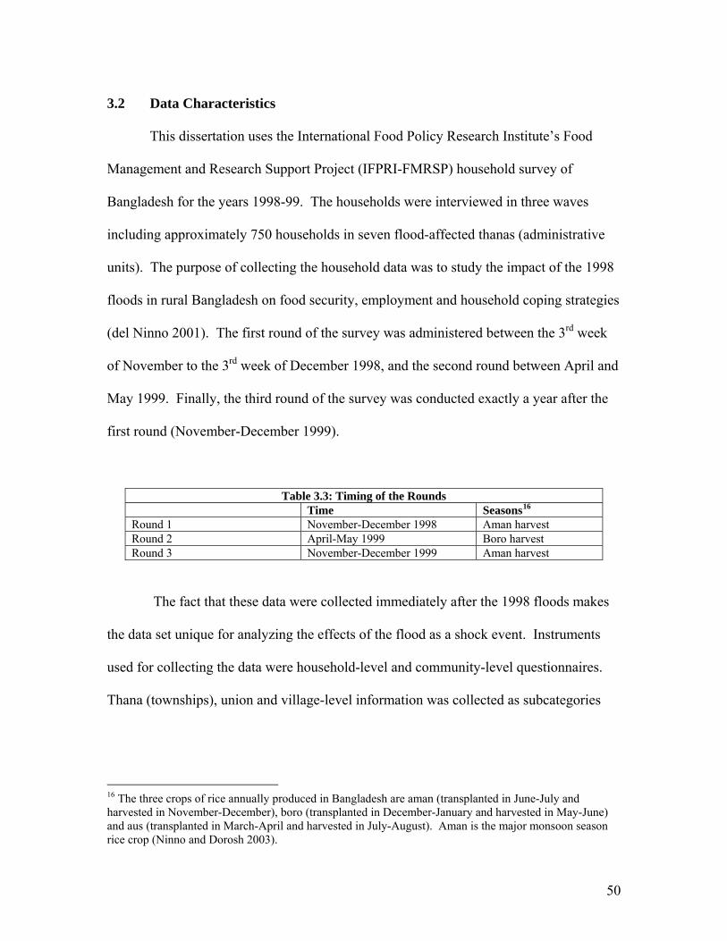
Table 1.1 Types of risks faced by the households 4Table 1.2 Policy instruments for risk reduction 5Table 1.3 Trends in poverty and inequality in the 1990s in Bangladesh 10Table 2.1 Five-tier classification of the poor 21Table 2.2 Studies decomposing the poor into relevant categories 24Table 3.1 Country profile 44Table 3.2 Division profile 48Table 3.3 Timing of the rounds 50Table 3.4 Summary of the content of the household and community-level

questionnaire 52

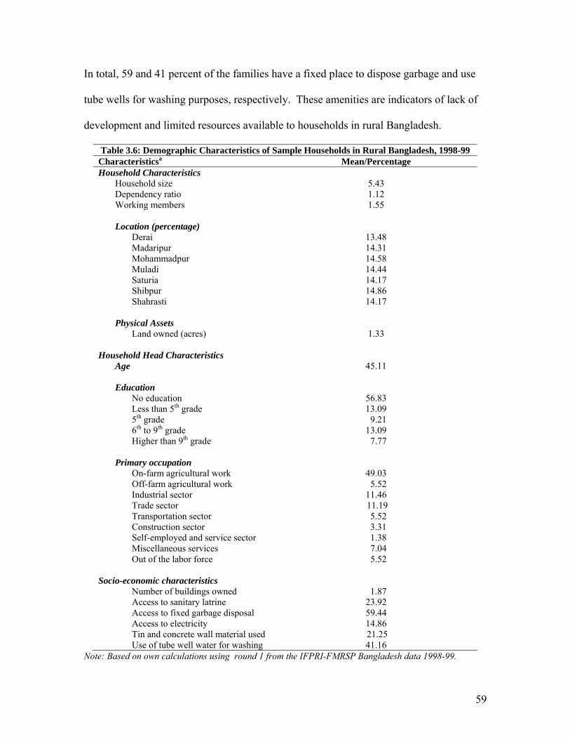
Table 3.5 Selected Thanas 53Table 3.6 Demographic characteristics of sample of households in rural

Bangladesh, 1998-99 59

Table 3.7 Financial Asset ownership of sample households in rural Bangladesh, 1998-99

60

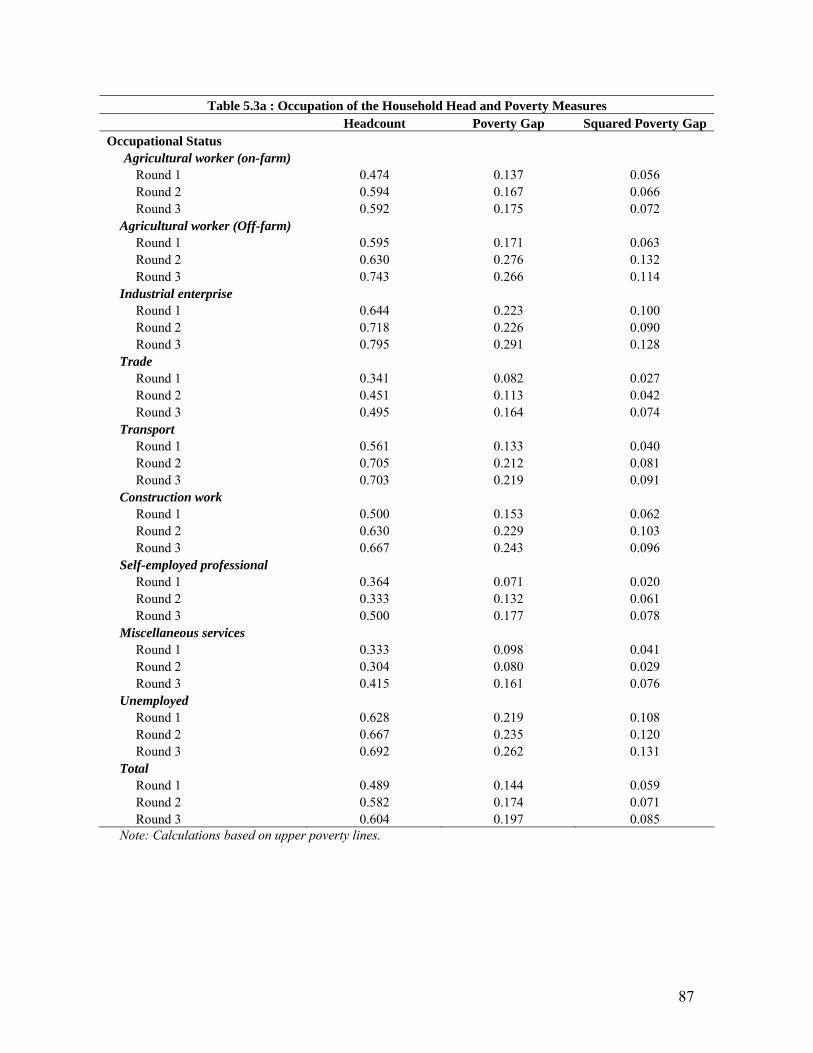
Table 3.8 Amount of credit taken by gender and region 65Table 4.1 CBN region poverty lines 75Table 5.1 Consumption expenditure and poverty 85Table 5.2 Number of periods poor 86Table 5.3a Occupation of the household head and poverty measures 87Table 5.3b Educational attainment of the household head and poverty measures 88Table 5.3c Age and gender of the household head and poverty measures 89Table 5.4 Area under the ROC curve for individual poverty indicators and over

all model using upper poverty line 94

Table 5.5 Number of poor in Bangladesh by poverty categories 96Table 5.6 Characteristics of sample households in rural Bangladesh 100Table 5.7 Estimates and marginal effects from multinomial logistic regression:

persistent and sometimes poor 105

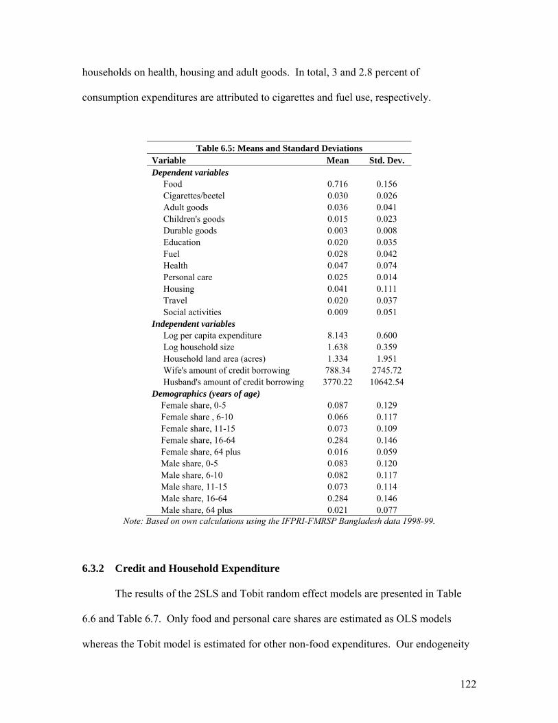
Table 5.8 Total, chronic and transient poverty by region 107Table 5.9 Censored quantile regression results (85th quantile) 109Table 6.1 Number of households in which men, women or both take loans 116Table 6.2 Formal and informal loans amount by head and spouse 117Table 6.3 Use of informal credit (%) 120Table 6.4 Use of formal credit (%) 121Table 6.5 Mean and standard deviations 122Table 6.6 Effect of credit amount on household expenditure shares, OLS and

Tobit estimates 126

Table 6.7 Effect of credit (dichotomous) on household expenditure shares, OLS and Tobit estimates

131

viii

List of Figures

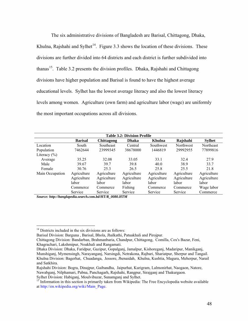
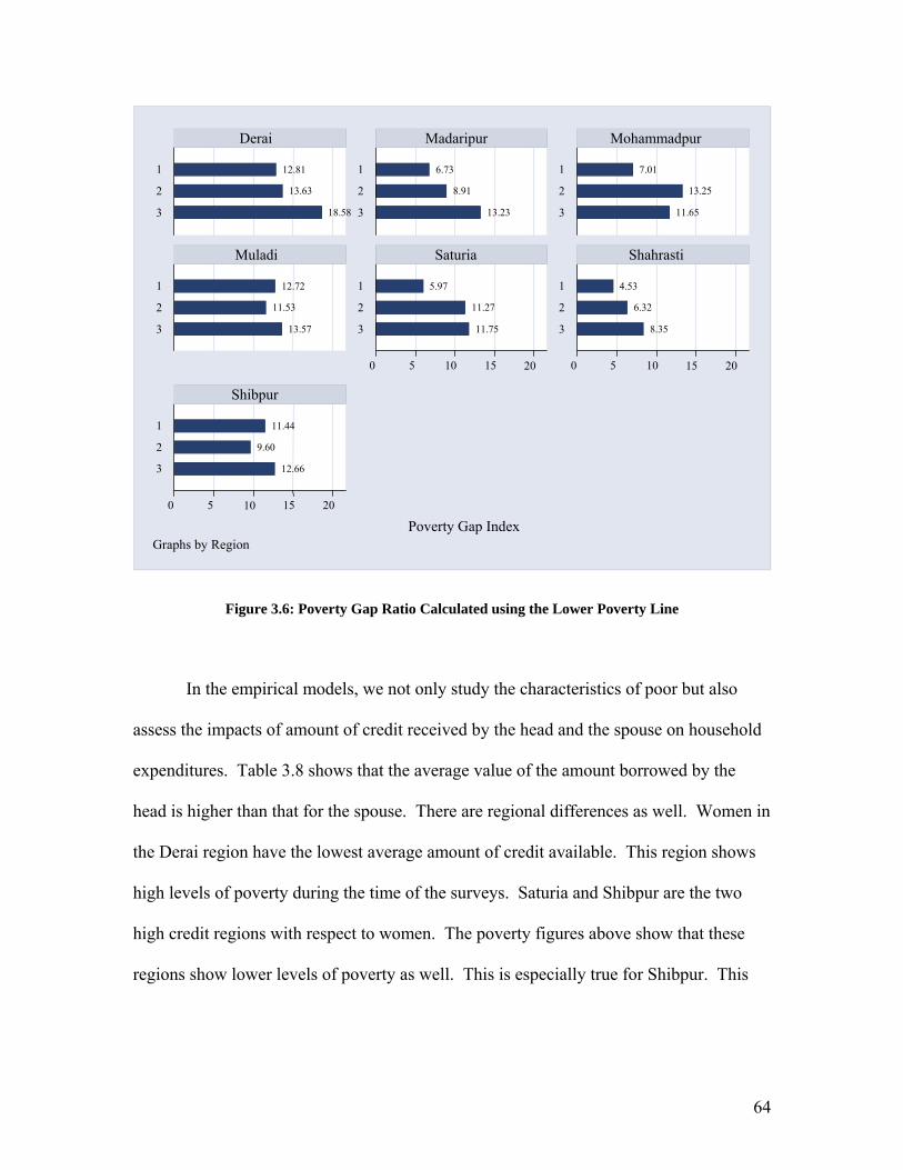
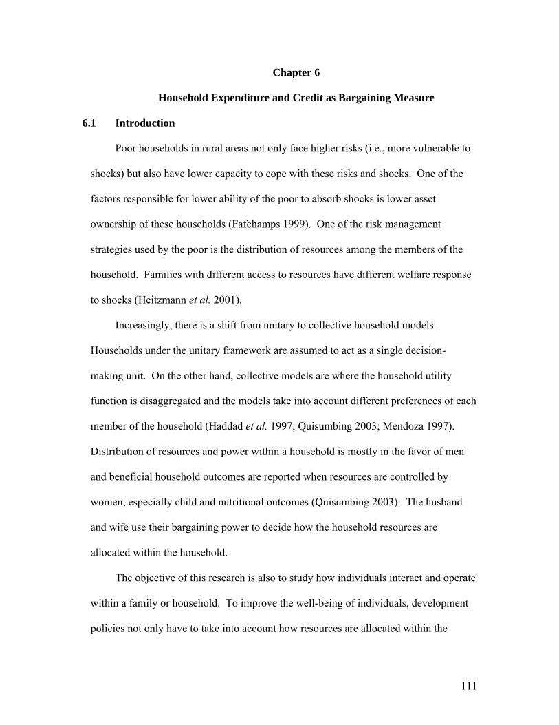
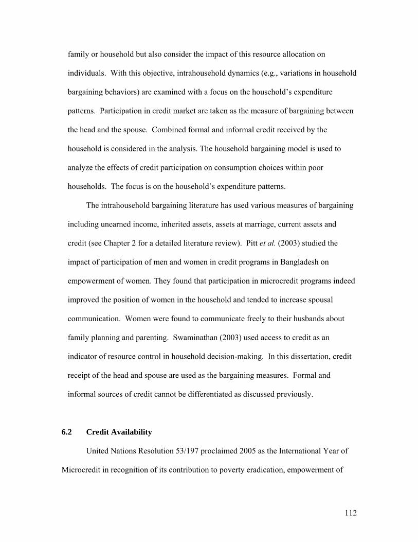
Figure 3.1 Political map of Bangladesh 45Figure 3.2 Flood affected area in Bangladesh 47Figure 3.3 Administrative divisions of Bangladesh 49Figure 3.4 Mean Consumption levels by lower poverty line 61Figure 3.5 Head count rate calculated using the lower poverty line 63Figure 3.6 Poverty gap ratio calculated using the lower poverty line 64Figure 3.7 Squared poverty gap ratio calculated using the lower poverty line 65Figure 5.1 Stochastic dominance curve 91Figure 5.2 ROC curve for poverty models 93Figure 6.1 Credit receipt of household head and spouse 117Figure 6.2 Food expenditure share by region 119Figure 6.3 Non-food expenditure shares by region 119

ix

Acknowledgements

I express my sincere gratitude to my advisor Prof. Jill L. Findeis for making this

dissertation possible. She has trained me to be a good researcher and also helped me

become a better person. Her deep commitment and optimism to research has been a

constant source of inspiration. I am grateful to each of my committee members; Profs.

Gretchen Cornwell, Bee-Yan Roberts, Carolyn Sachs, and Steve Smith for their support

and help. I would especially like to thank Prof. Cornwell for encouraging me to

undertake a qualitative study in Bangladesh. This study was funded by grants from the

Office of International Programs, College of Agricultural Sciences; Population Research

Institute; Women in Science and Engineering Institute; and the Department of

Agricultural Economics and Rural Sociology. The focus group discussions would not

have been possible without the help of Bangladesh Institute of Development Studies and

in particular Mr. Mohammad H.R. Bhuyan. I have also benefited from numerous

discussions with Hema and Tesfayi. I am extremely grateful to Prof. Francis Dodoo for

providing me with funding during the final stages of my dissertation.

I would like to thank my parents, Gita and Jayaraman for encouraging me to come

to Penn State and pursue my dream. They have prayed for my success and happiness. I

am grateful to my husband Chandrasekhar for all the help and support. Life in State

College would not have been fun without my good friends: Abhiroop, Priya, Smita, Ram,

Viji and Julia. I would also like to mention Meenakshi, Rajesh, Vijay and Anuja for

helping me at every stage. Finally, a word of thanks to Durga Athai for constant supply

of goodies!

x

1

Chapter 1

Research Problem

1.1 Introduction

South Asia has the largest concentration of the worlds’ poor1, with over half a

billion people surviving on less than a dollar a day. One of the Millennium Development

Goals (MDG) is halving the proportion of the world’s people whose income is less than

one dollar a day and the proportion of people who suffer from hunger by the year 2015

(OECD 2001). The success of poverty alleviation programs in South Asia is critical if

this MDG is to be met. Within South Asia, Bangladesh has the highest incidence of

poverty and only India and China have larger numbers of poor people. It is estimated

that nearly half of Bangladesh’s population of 135 million people live below the poverty

line (World Bank 2003a).

The United Nation’s General Assembly declared 1996 as the International Year

for the Eradication of Poverty. This was done "recognizing that poverty is a complex and

multi-dimensional problem with origins in both the national and international domains,

and that its eradication in all countries, in particular in developing countries, has become

one of the priority development objectives for the 1990s in order to promote sustainable

development.” (United Nations’ General Assembly Resolution 48/183 1993: p. 1). The

World Bank Group defines poverty as a multidimensional phenomenon where to be poor

not only means to be hungry and to lack access to shelter and resources but also means to

be illiterate, have poor health, not receive adequate nutrition and be vulnerable to shocks,

violence and crime. Not being in poverty entails individuals leading a life free from 1 Poverty is still a global problem in the 21st century, with 2.8 billion people living on less than $2 a day and 1.2 billion living on less than $1 a day (World Bank 2001b).

2

anxiety (World Bank 2001a, OECD 2001). Poverty has also been defined as the

combination of two interacting deprivations, namely physiological and social (Hazell and

Haddad 2001). Physiological deprivation includes deprivation resulting from lack of

income, food, education, shelter, sanitation and health. It can be quantified, and

household-level data capturing physiological deprivation are frequently collected and

readily available. Social deprivation is difficult to quantify because it includes elements

such as autonomy, time information, dignity and self-esteem (Hazell and Haddad 2001).

The traditional method of measuring poverty is to use the consumption or income

concept (defined as income poverty). An individual is deemed poor if his/her

consumption or income falls below the set minimum. The poverty line sets this

minimum standard specific to each society (Lipton and Ravallion 1995). Poverty has

different implications for individuals, families and societies. The International Labor

Organization defines different levels of poverty: individual, family and society-level

poverty (ILO 2003). Poverty results in poor health, lower working capacity, lower

productivity and a shorter life expectancy among individuals, and for families it leads to

inadequate schooling and income, early parenthood, poor health, and often early death.

At the societal level, poverty is an impediment to growth, stability and sustainable

development.

According to Hulme and Shepherd (2003), policy makers often define the poor as

those individuals who have not been integrated into the market economy and policy goals

often tend to view the poor as belonging to a single homogeneous category. Further,

policy makers tend to focus on only those poor whom the market can help (Hulme and

Shepherd 2003). Given that poverty alleviation is one of the most important challenges

3

faced by the international community today (ILO 2003), an understanding of the

dynamics of poverty alleviation is critical to the formulation of appropriate policy.

Poverty measures such as the head count ratio2 are static measures that are useful for

gauging the prevalence of poverty but do not indicate the severity of poverty or

fluctuations in economic welfare indicators over time including (but not limited to)

income and consumption.

1.2 Poverty and Vulnerability to Shocks

It is clear that one of the most important aspects of poverty is vulnerability. The

poor are the most vulnerable to health hazards, economic downturns, natural

catastrophes, and even man-made violence (World Bank 2001b). The World Bank

defines vulnerability as the likelihood of being affected by shocks, which have negative

impacts on the income and consumption of poor households. Further, households in most

developing countries face a high level of income variability due to factors beyond their

control, and their poverty makes them particularly vulnerable to shocks.

Shocks can be common or idiosyncratic. Common (or aggregate) shocks are

experienced by everyone in a particular group, community or geographical region while

an idiosyncratic shock affects only a particular individual or household (Dercon 2001a).

2 The most basic measure of poverty is the head count, which is the count of the poor below the poverty line. The head count index is the head count of those in poverty as the fraction of the total population. Other measures are the poverty gap index and the squared poverty gap index (Ray 1998). The depth of poverty is measured by the poverty gap index that calculates the average income shortfall from the poverty line. The squared poverty gap index measures the severity of poverty taking into account both distance separating the poor from the poverty line and income inequality (Ray 1998). These measures can be represented using the following equation where z is the poverty line, y is per capita expenditure and N is population size (World Bank 2002b): Pα= Σ [(z-y)/z]α/N with α = 0, 1 or 2, where α = 0 gives the head count index, α = 1 gives the poverty gap index and α = 2 gives the squared poverty gap index.

4

Table 1.1 categorizes the types of risks faced by individuals, households, communities

and geographical regions. Risks can be classified based on the level at which they occur

(micro, meso and macro) and can also be classified on the basis of type: natural, health,

social, economic, political and environmental (World Bank 2000). At the micro level,

individuals or specific households face a particular set of micro-level shocks focused at

the individual or household level, e.g., old age or domestic violence. Meso-level shocks

include shocks to groups of households or villages (for example, excessive rainfall,

landslides and epidemics), and national and international shocks are best classified as

macro shocks (World Bank 2000).

Table 1.1: Types of Risks Faced by Households Type of risk Risk affecting

individual or households (micro)

Risk affecting groups of households or

communities (meso)

Risk affecting regions or nations (macro)

Natural Rainfall, landslide, volcanic eruption

Earthquake, flood, drought, high winds

Health Illness, injury, death, disability, old age,

Epidemic

Social Crime, domestic violence

Terrorism, gang activity Civil strife, war, social upheaval

Economic Unemployment, resettlement, harvest failure

Change in food prices, growth collapse, hyperinflation, balance of payments, financial or currency crisis, technology shock, terms of trade shock, transition costs of economic costs

Political Riots Political default on social programs, Coup d’etat

Environmental Pollution, deforestation, nuclear disaster

Source: World Bank 2000.

5

While common shocks such as drought and floods increase the hardships

experienced by the poorer households, idiosyncratic shocks like illness, accidents and

death also have a deleterious impact on the economic well-being of households more

generally. There is a growing literature examining the impacts of shocks on poor

households (Fafchamps 1999; Dercon 2001a; Heitzmann et al. 2001). The World Bank

(2002a) cites a study of South Indian villages which showed that “the higher risk repre-

sented by a shift in the onset of the monsoon could cut the farm profits of households in

the lowest wealth quartile by 35%, compared to a 15% reduction for median households

and no effect on the wealthiest” (World Bank 2002a: p. vii).

Table 1.2: Policy Instruments for Risk Reduction Source of risk Spreading

awareness Public health, safe water & sanitation

Labor standards, workplace safety

Education & training

Natural disasters √ Epidemics √ √ Illness, disability √ √ Old age √ Economic crises Labor market risk √ √ Harvest failure, food price

Crime & violence √ √ Environmental resettlement

√ √ √

Source of risk Access to agro-

technology Sound macro-economic policy

Transparency in decision making

Redistribution, e.g. land reform

Natural disasters Epidemics Illness, disability Old age Economic crises √ √ Labor market risk √ √ Harvest failure, food price

√ √ √

Crime & violence Environmental resettlement

√

Source: World Bank 2002a: p. 15.

6

Table 1.2 suggests potential policy instruments to reduce risks. These instruments

promote growth, increase the quality of human capital and reduce poverty. Public

awareness could play an important role in helping individuals and households to cope

with natural disasters, epidemics, crime and violence, and environmental resettlement.

The table also indicates that having a sound health, education and macro-economic

infrastructure provides a cushion against various shocks and risks such as economic

crisis, crop failure, labor market risks and epidemics (World Bank 2002a).

Kochar (1995), while analyzing idiosyncratic crop shocks faced by agrarian

households in India, found that well-functioning labor markets and not credit markets

helped farmers to smooth consumption. These households were able to increase the

number of hours of work and thereby avoid depleting their savings and the selling off of

assets. Dercon and Krishnan (2000) observed high seasonal variability in consumption

and poverty in short-panel data from Ethiopia. They attribute the variability to the

presence of shocks. Households were found to be prone to both common shocks

(rainfall) and idiosyncratic shocks (household-specific crop and livestock shocks).

Dercon and Krishnan (2000) found that poverty transitions during the period under study

could be explained by people’s vulnerability to shocks and seasonal incentives in terms

of prices and employment opportunities that affected household consumption.

Households employ various coping strategies once affected by a shock, as they

attempt to return to their original level of consumption. Disinvestment is a popular

means of coping. Liquid assets such as jewelry are initially disposed, followed by more

productive assets, making it increasingly difficult for households to return to their pre-

crisis state. Intensity, frequency and length of the shock have different impacts and

7

require different consumption-smoothing strategies. Consumption smoothing becomes

increasingly difficult for households with successive shocks (Alderman 1996). Poor

agrarian households are most susceptible to climatic shocks that directly affect crop

production and indirectly affect labor income. Household savings, asset accumulation,

income diversification, reallocation of labor, temporary migration and group-based risk

sharing are among the coping strategies used by households (Fafchamps 1999).

1.3 Shocks in Bangladesh

In 1998, Bangladesh experienced one of the largest floods of the century, which

covered more than two-thirds of the country and caused a loss of 2.04 million metric tons

of rice crop (del Ninno et al. 2001). While the overall economic impact of this flood was

less severe than previous flood occurrences and caused less damage than anticipated

(Benson and Clay 2002), the floods significantly damaged the crops and other productive

assets and further contributed to underemployment. Fortunately, trade liberalization in

the early 1990s made large-scale private food imports possible, and government food

transfers and non-governmental organization activities averted a major food crisis in

Bangladesh. However, there were short-term and medium-term negative impacts

attributable to the major flooding that occurred. In the short-term, consumption declined

and there were observed increases in the incidence of illness, especially among children.

The medium-term impact was an increase in private borrowing and negative impacts on

nutritional intake (del Ninno et al. 2003).

In Bangladesh, the agricultural sector and the labor market were the most

negatively affected after the 1998 flood. Households coped by growing alternative crops

8

and feeding alternative feed to livestock, and by finding alternative employment

opportunities. Private borrowing, used mainly for buying food, was the most widely used

coping mechanism relied on by Bangladeshi households (del Ninno et al. 2001).

Subsequent food insecurity resulted in households buying food on credit, reducing food

consumption, and borrowing money to buy food. The resulting changes in food

consumption had health implications, especially among children: an increase in stunting

and wasting among Bangladeshi preschoolers was observed (del Ninno et al. 2003).

Admittedly, shocks are an integral part of a developing economy and policies

should be geared towards equipping the poor to cope. The standard policy prescriptions

aimed at poverty reduction typically focus on ways to improve the mean utility of a poor

household. In contrast, policies that reduce the variance of households’ well-being over

time are becoming increasingly popular. Here a distinction is being made between

policies aimed at reducing chronic poverty and those to reduce transient poverty. The

World Bank (2002a) recommends a social protection strategy that extends “beyond the

traditional poverty reduction measures, to focus on creating opportunities for households

to manage risk better, primarily through a variety of instruments that perform the role of

safety nets” (World Bank 2002a: p. vi).

1.4 Poverty in Bangladesh

Bangladesh has received considerable international focus because of its high

density of population and low income. It is recognized as one of the most disaster-prone

countries in the world (Benson and Clay 2002). These factors make Bangladesh one of

the most vulnerable societies in the world. From the time of its independence in 1971,

9

Bangladesh has made considerable progress on all fronts (World Bank 2003b). The

country has achieved commendable reductions in population growth rates, child mortality

and child malnutrition (World Bank 2002b). There has also been successful disaster

management, increasing emancipation of women and growth of grass-root activism

through Non-government Organizations (NGOs) and Community-based Organizations

(CBOs) (World Bank 2003b).

There has been a reduction in both ‘income poverty’ and ‘human poverty’ in

Bangladesh since independence3. Human poverty in Bangladesh has declined at a faster

rate than income poverty in the past two decades but income poverty reduction has been

faster in the 1990s compared to the 1980s. Overall income poverty has declined at the

rate of 1 percent per annum (World Bank 2003b). Despite this progress, there has also

been an increase in inequality, both income and gender, during this period.

The difference in poverty between the poor and the poorest group is stark, where

45 percent of the poor live in extreme poverty4. Further, extreme poverty is higher

among female-headed or female-managed households. Table 1.3 shows that while all

poverty measures declined from 1991-92 to 2000, the Gini index of inequality indicates

an increase in income inequality in Bangladesh over this time period (World Bank

2003b).

3 Taking into account the multidimensionality of poverty, it is possible to categorize it into income poverty and human poverty. Income poverty measures poverty in quantitative terms. Over the 1990s, there has been increase in consumption expenditure, that is, a decline in income poverty (World Bank 2003b). The concept of human poverty was first defined in UNDP’s Human Development Report in the year 1997. It focuses on what people can or cannot do. The human poverty index captures health, literacy and economic provision deprivation (UNDP 2000). 4 Extreme poverty is defined as taking less than 1800 Kcal as per the direct calorie measure (World Bank 2003b).

10

Table 1.3: Trends in Poverty and Inequality in the 1990s in Bangladesh 1991/92 2000 Change per year (%)

Headcount Rate National Rural Urban

58.8 44.9 61.2

49.8 36.6 53.0

-1.8 -2.2 -1.6

Poverty Gap National Rural Urban

17.2 12.0 18.1

12.9 9.5

13.8

-2.9 -2.5 -2.8

Squared Poverty Gap National Rural Urban

6.8 4.4 7.2

4.6 3.4 4.9

-3.8 -2.7 -3.8

Gini Index of Inequality National Rural Urban

0.259 0.307 0.243

0.306 0.368 0.271

2.1 2.3 1.4

Source: BBS, Preliminary Report of Household Income and Expenditure Survey 2000, Dhaka, 2001 and World Bank, op.cit.(World Bank 2003b).

Roughly half of Bangladesh’s population still lives in extreme poverty (World

Bank 2002b). Poverty declined by 9 percent over 1990-2000 but the absolute number of

poor remained stable because of population growth. It is the eighth most populous

country in the world, with a total population of 135.7 million and a population growth

rate of 1.7 percent per annum in 2002 (World Bank 2004).

There have also been changes in the structural composition of the Bangladeshi

economy. During the 1990s, the share of agriculture in the Gross Domestic Product

(GDP) declined and that of the service and manufacturing industry sectors increased.

Structural adjustments in terms of trade liberalization since the 1980s brought about

macroeconomic stability, improved fiscal and monetary management and encouraged

private sector investment in the economy (Benson and Clay 2002). The question

becomes, given these important changes in Bangladesh, how can the vulnerability of

these households be reduced so as to better adjust to exogenous shocks. Among

Bangladesh’s poor, this is a critical question.

11

1.5 Consumption Smoothing

Provision of a safety net should include availability of credit to the rural

households. Ray (1998) divides credit requirements into fixed capital, working capital

and consumption credit. He defines fixed capital as the credit required for investment in

new production units which could be used to cover the fixed cost of the units. Working

capital includes costs of day-to-day running of the unit and finally, consumption credit

includes credit needed by the poor to smooth consumption due to shocks. This type of

credit need arises in agrarian societies where seasonality dictates earnings of the

households. Among the consumption smoothing mechanisms, consumption credit is

most prominent in the developing world and most of it is informal (Fafchamps 1999).

Credit could come from formal or informal sources. Formal sources include government

banks, commercial banks and NGOs and informal sources include borrowing from a local

money lender, landlord, friends and neighbors. Informal credit markets are found to

charge high, exploitative interest rates but play an important role in rural credit markets.

Other income-smoothing mechanisms used by households are remittances and transfers

from family, friends and other institutions such as NGOs. These could be viewed as

returns to social capital (Dercon 2001a).

Policy makers in the developing world have found it difficult to provide access to

credit to small rural borrowers and microfinance is an attempt to reach the poor deprived

of financial services (UNCDF 2005). In Bangladesh, microcredit programs play an

important role and these programs focus on the poor. An estimated 13 million poor

people benefit from microfinance and credit availability in Bangladesh (UNCDF 2005).

NGOs have become actively involved in the microfinance sector. The four large

12

institutions that play a crucial role in this sector are BRAC (Bangladesh Rural

Advancement Committee), Grameen, Association for Social Advancement (ASA) and

Proshika (Zaman 2004).

Zaman (2004), in his exposition of the evolution of the microfinance sector in

Bangladesh, observes that the earliest microcredit models came about in Bangladesh in

the 1970s in an attempt to rehabilitate people post-independence. The 1980s witnessed

growth in NGO in the provision of credit and which subsequently in the 1990s developed

into the ‘Grameen-model’ of credit delivery. The majority of borrowers are women who

are targeted by these programs. Individuals receive loans as members of a group. Group

liability ensures repayment and extending credit to women also has an element of

empowerment. Kabeer (2001), in her evaluation of empowerment potential of credit

programs in rural Bangladesh, finds improvement in household outcomes when women

are given loans but cautions that patriarchal society in Bangladesh is still a constraint for

women.

Focused leadership and supportive legal systems have contributed to the success

of the microcredit movement (Morduch 1999). It is argued that these formal financial

services do not reach the poorest of the poor. In Bangladesh, microfinance prominence is

lowest among the poorest group and highest among the second lowest quintile group

(Hashemi and Rosenburg 2006; Morduch 1999). These programs have improved the

lives of poor households but it is important to note that they are costly to implement and

need to be heavily subsidized (Morduch 1999).

13

1.6 Gender and Poverty

Individuals interact and operate within a family or household. To improve the

well-being of individuals, development policies not only have to take into account how

resources are allocated within the family or household but also the impact of this resource

allocation on individuals. This process of resource allocation and the resulting outcomes

are referred to as “intrahousehold resource allocation” (Haddad et al. 1997; Quisumbing

2003). Differential intrahousehold resource allocation has implications for inequality and

poverty among household members (Strauss and Beegle 1996).

Numerous studies have shown that equality of men and women in a society has

positive effect on growth of the economy, poverty alleviation and individual well-being

of household members. Productive assets in the hands of the women have led to

reduction in poverty levels and empowerment of women (World Bank 2002c).

Empowerment indicators include both participation in the political process and control

over household resources. Access to credit and financial resources are limited for women

especially in rural areas (Bamberger et al. 2002). Moreover, the intrahousehold resource

allocation literature supports the fact that transfer of resources improves the bargaining

position of women in the household and thereby improves resource allocation and child

outcomes.

As part of this research focus group discussions were held in Bangladesh. The

rationale for the focus groups was to explore not only the coping strategies employed by

the households during and after floods but also to see if there was evidence of any form

of bargaining within the household. These discussions raised a number of questions:

What decision making power did the wife have in the household? Did that affect

14

intrahousehold resource allocation? Did receipt of credit or any other form of resource

give her more power to make decisions in the household? Could the decisions taken in

the household be gender differentiated? The qualitative study was not only important in

understanding the social and cultural context in Bangladesh and therefore helped in better

interpretation of the empirical results but also indicated that receipt of financial help

could possibly increase women’s say in family matters. They also pointed that that

borrowing money especially from informal sources was one of the major coping

mechanisms employed by Bangladeshi households.

1.7 Study Objectives

Given this perspective, this research analyzes issues related to chronic and

transient poverty following a major catastrophic (flood) event using a short panel of

household data from Bangladesh. This analysis is at the household level where the

research examines how the poverty level changes and how poor and non-poor families

are different from each other. Households have been found to adjust to shocks such as

floods by borrowing, selling assets and altering expenditures (del Ninno et al. 2001).

Among these coping mechanisms, we focus on credit receipt by the household head and

the spouse and the resultant differential household-level outcomes. Here the focus is on

individuals in the household and an attempt is made to study how their interaction affects

household resource allocation. The data used in this study were primarily collected to

identify policy prescriptions for sustainable improvement in household food security in

the period following the 1998 Bangladesh flood. The specific research objectives are:

15

1 To identify the determinants of poverty in Bangladesh, with a specific focus on

differentiating those who experienced poverty following the 1998 flood in

Bangladesh and those who did not.

2 To determine the differences between those among the poor (identified in

objective 1) who are able to eventually escape poverty following the flood (the

transient poor) versus those unable to leave poverty (chronic poor). It is

hypothesized that the poor are heterogeneous and within the poverty group those

who endure poverty for a sustained period of time are characteristically different

from those who move into and out of poverty.

3 To understand how intrahousehold dynamics (e.g., variations in household

bargaining behaviors) lead to differences in outcomes of specific interest (e.g.,

food expenditure). The household bargaining model will be used to analyze the

effects of receipt of credit on consumption choices within these poor households

following the flood event. The focus is on the household’s expenditure patterns.

The study hypothesizes that receiving credit from formal and informal sources

will affect decision-making capacity of women in Bangladeshi households. This

in turn is expected to have implications for child health and nutritional outcomes.

It is important to point out that the study is not looking at how the credit amount

is spent by the receiver but instead assesses how household expenditure patterns

are associated with credit receipt by the husband and wife. Availability of data on

credit receipt by individual members of the household enables us to look at

gender differentials resulting from transfer of resources in the hands of women.

16

We also restrict our analysis to male-headed households since there are too few

female-headed households in our data.

1.8 Organization of the Dissertation

Following this introduction, Chapter 2 of the dissertation provides a review of

literature relating to poverty and the ability of households to cope with exogenous shocks.

It also addresses the bargaining literature and the theoretical model relevant for the

agricultural household. Chapter 3 presents country and data descriptions. Chapter 4

outlines the methods and the estimation strategy used in the dissertation. Chapter 5 and

Chapter 6 present the results of the analysis. Finally, Chapter 7 describes the research

conclusions and policy implications.

17

Chapter 2

Literature Review and Theoretical Framework

2.1 Introduction

The World Bank Group defines poverty as a multidimensional phenomenon

where to be poor not only means to be hungry and to lack access to shelter and resources

but also means to be illiterate, have poor health, fail to receive adequate nutrition and be

vulnerable to shocks, violence and crime. The poor can be divided into those who remain

poor continuously over time and those who enter and exit poverty from time to time. A

large proportion of the poor include people moving into and out of poverty (Baulch and

Hoddinott 2000). As noted in Section 1, the poor are the most vulnerable to health

hazards, economic downturns, natural catastrophes, and even man-made violence (World

Bank 2001a). The World Bank defines vulnerability as the likelihood of being affected

by shocks, which have negative impacts on the income and consumption levels of poor

households. Further, households in most developing countries face high income

variability due to factors beyond their control, and their poverty makes them particularly

vulnerable to shocks. Depending on how well households are able to cope, they could

remain in poverty or may be able to move out of poverty following the shock (Baulch and

Hoddinott 2000).

The coping strategies that result in consumption smoothing in response to a shock

reflect poverty dynamics5. Recent advances in computation coupled with the more

frequent collection of panel data at the household level have contributed to the study of

both the dynamics of poverty and the coping strategies that households use over time as

5 Poverty dynamics is defined as the movement into and out of poverty (Baulch and Hoddinott 2000).

18

they attempt to escape poverty. Recent studies of poverty, a topic widely covered in the

literature, have focused on the dynamics of poverty, including what it means to be in

poverty for the long term versus in the transient poverty state. At the same time, new

theories of household interactions have emerged in the economics literature, allowing

examination of intrahousehold effects. This section examines both of these topics – i.e.,

the recent literature that examines poverty dynamics, and in specific, chronic versus

transient poverty, and the literature on the new household models that focus on

intrahousehold behaviors.

2.2 Poverty Dynamics

The percentage of people living below the poverty line is an aggregate measure

that is useful in some respects but limited in others. A limitation of the aggregate

measures is their failure to provide any indication of how poor households are faring or

whether their economic status is changing over time. It is important to disaggregate the

poor to understand their circumstances and dynamics. It is critical to understand the

differences among the different types of households and individuals within households

who are classified as ‘poor’. One salient difference is the difference between those

households and individuals who move into and out of poverty versus those who fail to

move out of poverty over time. This calls for incorporating a dynamic perspective into

poverty analysis, with differentiation between the chronic and transient poor.

Households who experience poverty and deprivation for prolonged periods are

defined as chronically poor and those who move into and out of poverty (temporary) are

the transient poor (Hulme and Shepherd 2003). These two types of poverty require

19

different policy measures. Chronic poverty eradication measures include long-term

investments such as increasing human and physical capital and the returns to assets. On

the other hand, policies to help the poor cope with idiosyncratic shocks are appropriate to

tackle the problem of transient poverty. Understanding why households move into and

out of poverty can help to target the poor more effectively than assessing only static

welfare indicators; static measures may (wrongly) include those experiencing short-term

misfortunes but otherwise are not poor based on their permanent incomes or levels of

consumption. Similarly, excluding those experiencing only temporary spells out of

poverty but in fact who are in poverty the majority of the time is also a weakness (Baulch

and Hoddinott 2000). Baulch and Hoddinott (2000) emphasize that understanding factors

affecting poverty dynamics help in designing safety net policies and, most importantly,

help to target the vulnerable.

Finally, while income and consumption measures of poverty are often used to

study chronic and transient poverty, there is an increasing emphasis on adopting a

multidimensional approach in poverty studies by considering other measures such as

educational attainment, nutritional intake and ownership of assets in the analysis (McKay

and Lawson 2002).

2.2.1 Definition of Chronic and Transient Poverty

It is widely accepted that the poor are a heterogeneous group. Studies of poverty

dynamics generally treat a household as a single economic unit6. Jalan and Ravallion

(2000) define transient poverty as the poverty that is caused by variability in

6 Assumes a unitary model framework.

20

consumption. A household with mean consumption below the poverty line across all

periods is defined to be experiencing chronic poverty. Hulme and Shepherd (2003)

define the chronically poor as those who experience poverty for a period of five years or

more and transient poor as those who move into and out of poverty. They argue that the

five-year period is a significant length of time and studies show that individuals who are

poor for five years or more have a high probability of remaining poor for the rest of their

lives. The chronic poor suffer from persistent deprivation. The chronically poor are also

those who need external help to get out of the poverty trap and they remain poor despite

implementation of policies to tackle poverty (Aliber 2003). Chronic poverty also is

transmitted from one generation to another, and children within chronically poor

households are more likely to be caught in the poverty trap and likely to remain poor the

rest of their lives (Aliber 2003).

2.2.2 Measuring Chronic and Transient Poverty

Income and consumption7 measures at the household level are common measures

of chronic and transient deprivation and longitudinal or panel data sets are ideally suited

to study poverty movements or transitions8. However, the multidimensional definition of

poverty requires that other welfare indicators – for example, asset ownership, nutritional

intake, educational enrollment, the human deprivation index -- could be included to

provide a more inclusive measure of poverty.

Even households that are sometimes poor are heterogeneous. The question

becomes how to rigorously define the transient poor (Baulch and Hoddinott 2000). For 7 Also called metric welfare measure (Baulch and Hoddinott 2000). 8 Atleast a three-year panel data set is needed (Baulch and Hoddinott 2000).

21

example, using the definition that the chronically poor are poor continuously over time

and the transient poor experience at least one spell out of poverty, in five-year panel data,

a household classified as poor for four years would be categorized as transient poor but

then so would be a household that is poor just one year. Treating both households alike is

probably not reasonable. Hulme and Shepherd (2003) categorize poor as ‘always poor’,

‘usually poor’, ‘churning poor’, ‘occasional poor’ and ‘never poor’ (see Table 2.1). Both

income and non-income indicators are used in their categorization.

Table 2.1: Five-tier Classification of the Poor Aggregate category Specific category Definition Chronic poor

Always poor Usually poor

Those whose poverty score is below the poverty line for each period. Those whose mean poverty score over all periods is below the poverty line but not poor in every period.

Transient poor Churning poor Occasionally poor

Those with a mean poverty score around the poverty line and who are poor in some periods. Those with mean a poverty score above the poverty line and that have experienced at least one period of poverty.

Non-poor Never poor Those whose mean score is always above the poverty line.

Source: Hulme and Shepherd (2003).

The poverty literature delineates two approaches to study transitory and chronic

poverty using income or consumption data. First, the spells approach is used, where the

number or length of poverty spells experienced classifies the poor as chronic or transient

(McKay and Lawson 2002). A transition matrix can be used to provide information on

the proportion or number of people moving into and out of poverty using deciles,

quintiles or poverty lines, and also gives information about the poverty experiences of

22

households in the intervening period (Oduro 2002). Using this approach, Oduro (2002)

found that consumption measures are generally less variable compared to income

measure of poverty. This is because households have the ability to smooth consumption

over time. Therefore, the number of poor in the transient category increase when the

income measure of poverty is used and different welfare measure could yield different

estimates of transient and chronic poverty. The spells approach is plagued by

measurement error occurring in the process of collecting income and consumption data

(Hulme and Shepherd 2003). Difficulty in measuring the values of own production (as

well as problems recalling and imputing values) and in determining the revenue and cost

of farm and non-farm enterprises result in errors (Baulch and Hoddinott 2000).

A second approach, the components approach, decomposes the permanent component of

household income from its transitory variations. Households that have permanent

components below the poverty line are then defined as the chronically poor (McKay and

Lawson 2002).

It is recommended that to have a complete picture, the spells and component

approach based on income or consumption have to be complemented by the used of

qualitative studies. That is, there is a need to move beyond defining poverty in monetary

terms.

2.2.3 Empirical Studies

An important question is why some households are not able to move out of

poverty while others appear to move into and out of poverty over time – they escape

being poor but often fall back into poverty at least temporarily. Some studies have been

23

able to predict chronic poverty better than transitory poverty (Haddad and Ahmed 2003;

Baulch and Hoddinott 2000; Jalan and Ravallion 2000). Analysis of chronic poverty

across 25 countries shows that chronic poverty is spatially concentrated, affected by

demographic composition of the household and determined by human and physical

capital and labor markets (Yaqub 2002).

Jalan and Ravallion (2000) define total poverty as the sum of chronic and

transient poverty and decompose households into total, chronic and transient poor using

the squared poverty gap index. The censored quantile regression technique is used to

identify the determinants of both chronic and transient poverty. Their model is able to

predict chronic poverty better than transient poverty, with the determinants of chronic

and total poverty being similar. Haddad and Ahmed (2003), using a two-round panel

data set for Egypt, measure changes in per capita consumption among households. They

calculate squared poverty gap measures for each household and divide the sample

population into total, transient and chronically poor groups. The censored quantile

regression method is again applied to identify the determinants of chronic and transient

poverty. As was also true for Jalan and Ravallion (2000), their model predicts chronic

poverty better than transient poverty, with the determinants of total and chronic poverty

again being quite similar.

Kedir and McKay (2003) analyze three waves of household survey to study

chronic poverty in Ethiopia using total household expenditure per month as the welfare

indicator and the population is classified into ‘always poor’, ‘two-period poor’, ‘one-

period poor’ and ‘never poor’. Multinomial regression analysis indicates that household

24

composition, unemployment, lack of asset ownership, lack of education, ethnicity, and

the age and gender of the household head are important determinants of chronic poverty.

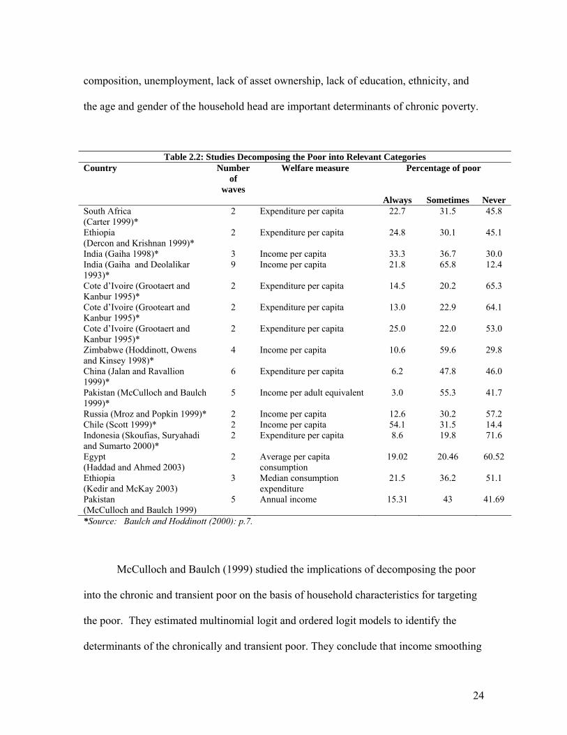
Table 2.2: Studies Decomposing the Poor into Relevant Categories Country Number

of waves

Welfare measure Percentage of poor

Always Sometimes Never South Africa (Carter 1999)*

2 Expenditure per capita 22.7 31.5 45.8

Ethiopia (Dercon and Krishnan 1999)*


India (Gaiha 1998)* 3 Income per capita 33.3 36.7 30.0 India (Gaiha and Deolalikar 1993)*

9 Income per capita 21.8 65.8 12.4

Cote d’Ivoire (Grootaert and Kanbur 1995)*


Cote d’Ivoire (Grooteart and Kanbur 1995)*


Cote d’Ivoire (Grootaert and Kanbur 1995)*


Zimbabwe (Hoddinott, Owens and Kinsey 1998)*

4 Income per capita 10.6 59.6 29.8

China (Jalan and Ravallion 1999)*


Pakistan (McCulloch and Baulch 1999)*

5 Income per adult equivalent 3.0 55.3 41.7

Russia (Mroz and Popkin 1999)* 2 Income per capita 12.6 30.2 57.2 Chile (Scott 1999)* 2 Income per capita 54.1 31.5 14.4 Indonesia (Skoufias, Suryahadi and Sumarto 2000)*


Egypt (Haddad and Ahmed 2003)

2 Average per capita consumption

19.02 20.46 60.52

Ethiopia (Kedir and McKay 2003)

3 Median consumption expenditure

21.5 36.2 51.1

Pakistan (McCulloch and Baulch 1999)

5 Annual income 15.31 43 41.69

*Source: Baulch and Hoddinott (2000): p.7.

McCulloch and Baulch (1999) studied the implications of decomposing the poor

into the chronic and transient poor on the basis of household characteristics for targeting

the poor. They estimated multinomial logit and ordered logit models to identify the

determinants of the chronically and transient poor. They conclude that income smoothing

25

policies are more appropriate for tackling the problem of transitory poverty while growth

policies designed to increase the mean income level help the poor to escape being

chronically poor. Table 2.2 provides a summary of selected studies of chronic and

transient poverty.

2.2.4 Characteristics of the Chronically Poor

Education is a powerful and important predictor of chronic poverty. Studies have

found that an increase in number of years of education decreases the probability of being

chronically poor (McCulloch and Baulch 1999; Jalan and Ravallion 2000; Aliber 2003;

McCulloch and Calandrino 2003). Human capital accumulation in Bangladesh is an

important form of asset holding for the poor, which equips them to participate in the

growth process (World Bank 2002b).

Larger households are more likely to experience chronic poverty. This is true

among households that have limited access to resources and assets. McCulloch and

Baulch (2000), Jalan and Ravallion (2000), Haddad and Ahmed (2003) and Aliber (2003)

in their study of Pakistan, China Egypt and South Africa, respectively, found this to be

true. Older household heads and female-headed households are also more likely to be

chronically poor (Aliber 2003). All things equal, the same is true for households with a

greater number of children, more members above the age of 60 and for households with

more disabled members.

Place of residence determines the opportunities and facilities available to the

households (McKay and Lawson 2002). Remote geographical locations are

disadvantaged in terms of access to resources. The likelihood of being persistently or

26

chronically poor in such locations is higher. McKay and Lawson (2002) also find that

chronic poverty is a major problem in rural areas because of lack of employment

opportunities and resources.

Lack of physical assets is associated with chronic poverty (McCulloch and Baulch

2000; Aliber 2003). Assets such as livestock and land help poor households not only

generate income but are also a form of investment. Poorer households commonly hold a

greater share of their assets in the form of liquid assets such as livestock and financial

assets (World Bank 2002a).

The sector of occupation of the household head is shown to be very important in

most studies. Haddad and Ahmed (2003), in their study of chronic and transient poverty,

report that being employed in the manufacturing, recreation or non-farm sectors

decreases the likelihood of being chronically poor as compared to being engaged in the

agricultural sector. Seasonal, casual and retrenched farm workers are also vulnerable

(Aliber 2003).

2.2.5 Characteristics of the Transient Poor

Some factors affect both chronic and transitory poverty but there are others that

are associated with transient poor alone. Poverty levels in general decline rapidly with

increases in education of the household head (World Bank 2002a). There is also a strong

negative association between transient poverty and educational attainment (Haddad and

Ahmed 2003; Jalan and Ravallion 2000). Jalan and Ravallion (2000) find higher

transitory poverty among smaller Chinese households. Adoption of new technology and

adverse price fluctuations can result in temporary poverty (McKay and Lawson 2002).

27

The adoption of new agricultural techniques involves risk taking on the part of farmers,

which, in turn, causes variability in their income. The study of Argentinean households

by Cruces and Wodon (2003) found that the risk of running a business made employers

vulnerable to transient poverty, and the provision of social security by the public sector

made households engaged in this sector more resistant to transient poverty.

2.3 Intrahousehold Resource Allocation Models

Individuals interact and operate within a family or household. To improve the

well-being of individuals, development policies not only have to take into account how

resources are allocated within the family or household but also the impact of this resource

allocation on individuals. This process of resource allocation and the resulting outcomes

are referred to as “intrahousehold resource allocation” (Haddad et al. 1997; Quisumbing

2003). Differential intrahousehold resource allocation has implications for inequality and

poverty among household members (Strauss and Beegle 1996).

2.3.1 Unitary Household Model

The traditional approach to intrahousehold resource allocation is the unitary

approach where the household is viewed as a single economic unit. Becker (1965)

proposed that the household, sharing a single set of preferences, maximized utility by

combining time, goods purchased in the market and goods produced at home. Becker’s

theory of time allocation assumes that households are both consumers and producers. As

producers, household combine nonlabor inputs and time using the cost minimization

approach and, as consumers, maximize their utility subject to prices and resource

28

constraints. Unitary models assume that all members of a household share the same

preference function and pool their resources. In Becker’s time allocation model,

households maximize the following utility function

U = U (Z1,…., Zm) ≡ U (f1,…., fm) = U (x1,….,xm; T1,…., Tm) [2.1]

where Zi are goods produced within the household, x1 is the vector of market goods, and

Ti is a vector of time inputs used in producing the ith commodity. The utility of the

household is maximized subject to:

1. Household production function which combines time and market goods to

produce goods:

Zi= fi (xi, Ti) [2.2]

The production function is characterized by fixed coefficients as:

T1 ≡ ti Zi [2.3]

xi ≡ bi Zi [2.4]

where ti is input of time required to produce one unit of household good (Z) and bi

is the input of market good required to produce a unit of household good (Z).

2. Goods constraint

∑m

tt xp1

= I = V + Tw ẅ [2.5]

where I is total income, V is other income, Tw denotes market work and ẅ is the

vector of wage rates.

3. Time constraint

Tc = T – Tw [2.6]

29

where T is the total time available during the day and Tc is the time spent on

consumption (leisure).

Equations 2.3, 2.4, 2.5 and 2.6 can be combined to yield the full-income constraint:

Σ (pibi+ t ẅ) Zi = V + T ẅ [2.7]

Households thereby make consumption and production decisions based on exogenous

factors, namely market prices, wages and non-earned income (Schultz 2001).

Apart from being applied to standard demand analysis, unitary models were

extended to include determinants of education, health, fertility, migration and labor

supply (Haddad et al. 1997). This approach is popular because it is straightforward and

household-level data are readily available. Attempts have been made to assess questions

of intrahousehold resource allocation within the unitary framework, despite its treatment

of households as ‘black box’ (Pitt 1997; Alderman and Gertler 1997). For example, Pitt

(1997) looks at household resource allocation using intrahousehold conditional demand

equations. These equations determine how allocations such as time and food to one

member affect allocations to others. This model requires prices of person-specific goods

for estimating demand equations. Absence of prices lead to issues of identification and

Pitt suggests solutions to overcome this problem. Further, Alderman and Gertler (1997)

use the unitary framework to show how gender plays a role in human capital investment

within households with different levels of resources. They find that the demand for

daughters’ human capital is more income and price elastic in cases where there is a son

preference. This was empirically tested in their study of Pakistan and expected

relationships were observed.

30

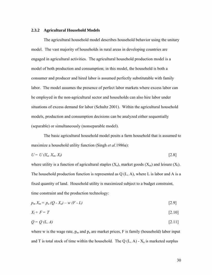
2.3.2 Agricultural Household Models

The agricultural household model describes household behavior using the unitary

model. The vast majority of households in rural areas in developing countries are

engaged in agricultural activities. The agricultural household production model is a

model of both production and consumption; in this model, the household is both a

consumer and producer and hired labor is assumed perfectly substitutable with family

labor. The model assumes the presence of perfect labor markets where excess labor can

be employed in the non-agricultural sector and households can also hire labor under

situations of excess demand for labor (Schultz 2001). Within the agricultural household

models, production and consumption decisions can be analyzed either sequentially

(separable) or simultaneously (nonseparable model).

The basic agricultural household model posits a farm household that is assumed to

maximize a household utility function (Singh et al.1986a):

U = U (Xa, Xm, Xl) [2.8]

where utility is a function of agricultural staples (Xa), market goods (Xm) and leisure (Xl).

The household production function is represented as Q (L, A), where L is labor and A is a

fixed quantity of land. Household utility is maximized subject to a budget constraint,

time constraint and the production technology:

pm Xm = pa (Q - Xa) – w (F - L) [2.9]

Xl + F = T [2.10]

Q = Q (L, A) [2.11]

where w is the wage rate, pm and pa are market prices, F is family (household) labor input

and T is total stock of time within the household. The Q (L, A) - Xa is marketed surplus

31

and F - L yields net sales of labor. All prices (w, pm, pa) are exogenous and the

household is a price-taker in all three markets. The three constraints are collapsed into

one full-income budget constraint:

pmXm + paXa + wXl = wT + paQ(L, A) – wL [2.12]

The paQ (L, A) – wL represents farm profits and the left-hand side of equation 2.12

represents total household expenditures including purchase of market goods, the

household’s purchase of its own output and its own purchase of time in the form of

leisure.

Optimal levels of consumption of each of the commodities (Xa, Xm, Xl) and the

total labor input utilized in agricultural production are determined. Optimal value of

labor, output and full income is derived solving the first-order conditions. In the case of

agricultural households, production activities determine income and factors affecting

production influence the household’s full income, which in turn affects household

consumption. Therefore, household production and consumption are separable or

recursive. Separability of the decision implies that production decisions are not

influenced by consumption and labor supply decisions but consumption and labor supply

decisions are dependent on production decisions. That is, production decisions do not

depend on consumption preferences but consumption decisions are influenced by

production through the full income. Households follow a two-step optimality procedure:

first, farm profits are maximized using the optimal combination of inputs and the

household utility function is maximized (Singh et al. 1986a).

Separable models are not applicable under all circumstances and nonseparable

models may be more appropriate in the case of presence of imperfect markets, when sale

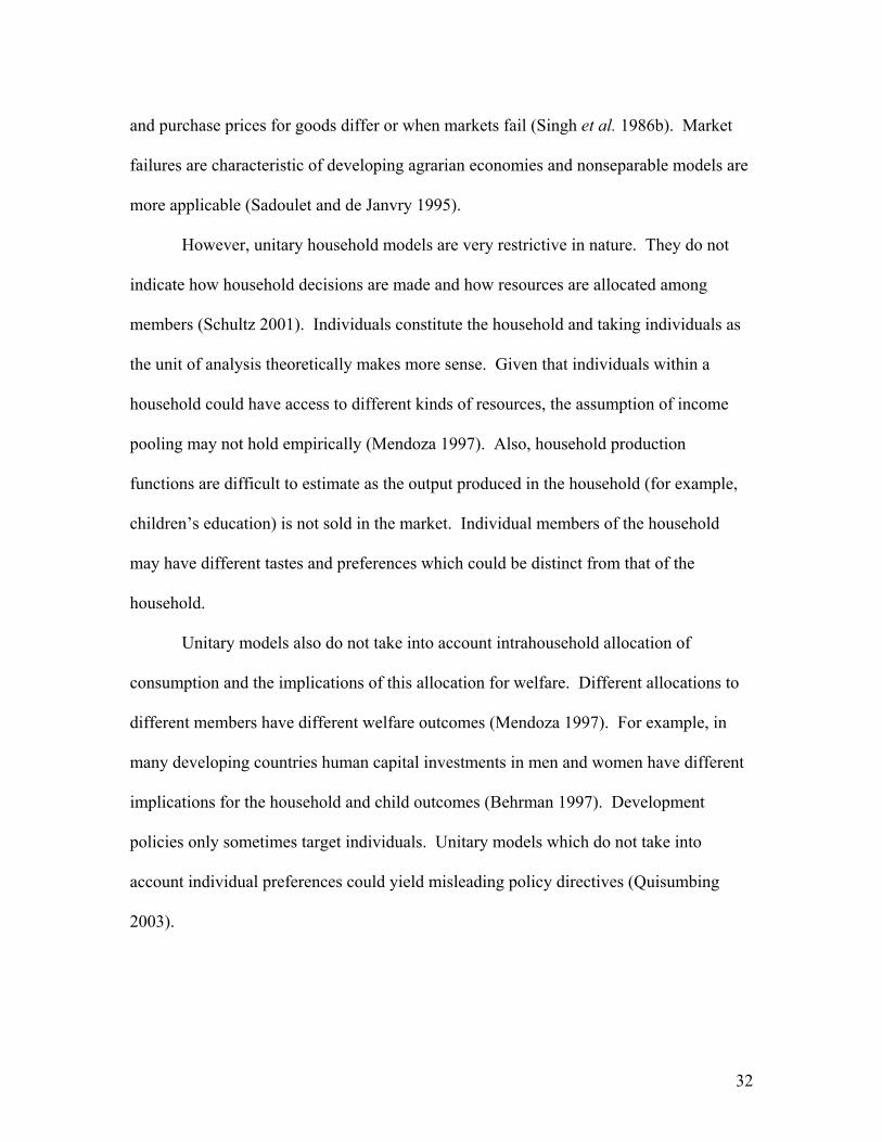
32

and purchase prices for goods differ or when markets fail (Singh et al. 1986b). Market

failures are characteristic of developing agrarian economies and nonseparable models are

more applicable (Sadoulet and de Janvry 1995).

However, unitary household models are very restrictive in nature. They do not

indicate how household decisions are made and how resources are allocated among

members (Schultz 2001). Individuals constitute the household and taking individuals as

the unit of analysis theoretically makes more sense. Given that individuals within a

household could have access to different kinds of resources, the assumption of income

pooling may not hold empirically (Mendoza 1997). Also, household production

functions are difficult to estimate as the output produced in the household (for example,

children’s education) is not sold in the market. Individual members of the household

may have different tastes and preferences which could be distinct from that of the

household.

Unitary models also do not take into account intrahousehold allocation of

consumption and the implications of this allocation for welfare. Different allocations to

different members have different welfare outcomes (Mendoza 1997). For example, in

many developing countries human capital investments in men and women have different

implications for the household and child outcomes (Behrman 1997). Development

policies only sometimes target individuals. Unitary models which do not take into

account individual preferences could yield misleading policy directives (Quisumbing

2003).

33

2.3.3 Collective Models

During the 1980s alternatives to the unitary approach to household resource

allocation emerged. Under the collective approach, the household utility function is

disaggregated and the model takes into account the different preferences of each member

of the household (Chiappori 1988, 1992; Browning and Chiappori (1998); Haddad et al.

1997; Quisumbing 2003; Mendoza 1997). Here the focus is on the individuals within the

household rather than on the entire household as one unit, and resources are no longer

pooled. Individuals decide the amount of their income to be transferred to others and the

amount allocated to purchasing common household goods (Doss 1996).

Unitary models can be shown as a special case of the collective models.

Collective household models can be divided into cooperative and non-cooperative models

(Mendoza 1997). All cooperative models assume that households make Pareto efficient

allocations, i.e., no one can be made better off without making someone else worse off

(Chiappori 1988, 1992) whereas non-cooperative models may or may not yield Pareto

optimal outcomes.

2.3.4 Cooperative Model

Cooperative models postulate that individuals form households only if there is a

net gain in doing so. There are two approaches within the cooperative framework. The

first approach assumes that all households have a sharing rule to allocate income among

members (Chiappori 1988, 1992; Browning and Chiappori 1998; Apps and Rees 1997).

The income-sharing rule is a function of the incomes of the husband and the wife and

total household income (Mendoza 1997). The household uses the sharing rule to allocate

34

resources among its members. Doss (1996) outlines four assumptions that are needed to

recover the sharing rule from household expenditure data: 1) requires that some goods be

private, 2) the utility of other members is included as one of the arguments in one’s own

utility function, 3) a separable utility function exists with respect to private and public

goods, and 4) at least one private good is assignable in order to observe who consumes

that good.

Browning et al. (1994) develop a model showing how income affects household

outcomes within the framework of family expenditure data. They assume that

households make Pareto efficient decisions and find that resource allocation decisions

among Canadian couples depend on their current income, age and lifetime wealth.

Browning et al. (1994) consider a two-member household (a, b) where households

maximize the weighted sum of household members’ utility subject to a budget constraint

(Strauss and Beegle 1996):

Max μ UA (xA, xB) + (1-μ) UB (xA, xB) [2.13]

subject to p (xA + xB) = Y [2.14]

where Ui is the utility function of the household members, xi is the private consumption

good, Y is total household income and p is the price vector for the market good. The μ is

the welfare weight for household member A which lies between 0 and 1 and is a function

of prices, household income and other factors such as the distribution of income (Strauss

and Beegle 1996). This model collapses into the unitary model if individuals A and B are

identical or if μ equals 0 or 1. This would imply that everybody has identical preferences

or there is a dictator in the household. Demand for the market good x is a function of

prices, income and μ (xA = xA (p, Y, μ (p, Y))).

35

Strauss and Beegle (1996) derive tests for the collective approach using a two-

stage decision process with an income-sharing rule. The household first pools resources

and allocates income to each individual and then individuals maximize their sub-utility

subject to the income they have been allotted. Suppose θ is the income allotted to one

member out of the total income Y, then in a two-member household the other member

would have (Y – θ) left for him/her. Therefore, in the second-stage, members maximize:

max UA (xA) [2.15]

subject to pxA = θ [2.16]

The sharing rule (θ) is a function of prices, income and other distributional factors and

the model is a unitary model when θ is fixed. The conditional demand curve is xA =

xA (p, θ). It is also postulated that the ratio of the marginal propensity to consume a good

with respect to changes in income of the two individuals is to be the same across all

goods. That is,

Bj

Aj

Bk

Ak

YXYX

YXYX

∂∂∂∂

=∂∂∂∂

//

// [2.17]

In a unitary model this ratio is equal to one and in a collective model this ratio represents

the sharing weights that determine the control of the individual over the resources.

Chiappori (1992) develops a collective model of household labor supply where the

economic agents first share nonlabor income based on the sharing rule and then in the

second-stage make labor supply and consumption decisions.

36

2.3.5 Cooperative Bargaining Models

The other approach was developed by McElroy and Horney (1981) and Manser

and Brown (1980) which explicitly assumes a bargaining rule among members of the

household. Manser and Brown (1980) provide a cooperative bargaining solution to the

issue of marriage and household decision-making where benefits derived from marriage

are distributed between the husband and wife. In the Manser and Brown model, a rule is

derived to resolve household allocative and distributional issues using a Nash-bargaining

model. Individuals have a guaranteed utility level that they enjoy when they do not

cooperate, and they marry or form a family only if the utility they derive from

cooperating is greater than being single. This minimum reservation utility is defined as

the threat point9 and gains from cooperation are a function of the bargaining strength of

the individual family members (Mendoza 1997). In the bargaining approach, control

over the income plays an important role in household decision-making unlike in Becker’s

unitary model where the household collectively controls the total income.

McElroy and Horney’s (1981) Nash-bargaining household decision model

assumes a two-individual household, m and f. Market goods of interest to m are

xm = (x0, x1, x3) at prices pm = (p0, p1, p3) and those of interest to f are xf = (x0, x2, x4) at

prices pf = (p0, p2, p4) where x1 and x2 are the market goods consumed by the husband and

the wife, respectively, and x3 and x4 are the leisure time10 of the husband and wife,

respectively. The x0 is the household good that is consumed which has a public good

characteristic. If individuals are not married then they maximize their individual utility

functions subject to their individual budgets, to derive their indirect utility functions 9 Defined as maximum level of utility outside of the household (McElroy 1990). 10 Leisure time is defined as time not spent in market work (McElroy and Horney 1981).

37

),(0 mmm

om IpVV = and ),(0 ff

fo

f IpVV = where Ik (k = m, f) is non-wage income.

Further, the McElroy and Horney model assumes gains from marriage, with the married

couple maximizing the Nash utility function

)];,()()][;,()([ 00 fffff

mmmmm IpVxUIpVxUN αα −−= [2.18]

subject to a full-income constraint

fm IITppxpxpxpxpxp +++=++++ )( 434433221100 [2.19]

where T is the time endowment of both individuals and the Vi are the threat points of the

individuals m and f (threat of becoming divorced). Threat points represent the utility

individuals would receive if they remain single (reservation utility) and the αi are the

extrahousehold environmental parameters (EEPs) (McElroy 1990). Solution to the

maximization problem yields Marshallian demand equations which are functions of

prices, nonlabor income, and the EEPs:

4,3,2,1,0),,;,,( == iIIphx fmfmii αα [2.20]

The EEPs shift the threat points and have no effect on nonwage income and prices

(McElroy 1990). They include social, legal and institutional parameters that have welfare

impacts on households, and thus enabling the policy component to be explicitly included

in the model (Swaminathan 2003). Examples of EEPs are divorce laws, welfare policies

of single mothers, extended family support networks and local ratios of marriageable men

to women (Schultz 2001). These factors may affect the reservation utilities and family

outcomes within the bargaining process.

Lundberg and Pollak (1993) introduce a ‘separate spheres’ bargaining model

within marriage. Divorce as a threat point is replaced by a non-cooperative equilibrium

38

that reflects traditional gender roles. Within this framework, Lundberg and Pollak (1993)

study the distributional implications of the child allowance schemes to the mother in

United Kingdom. This would make outcomes of cooperative bargaining favor the

woman. Ermisch (2003) suggests that an increase in mother’s income has an income

effect which gets translated into increases in expenditures on children and herself. This

also increases her bargaining power within the household. Assuming that women give

greater weight to children’s needs, improvement in her position could further increase

expenditure on children. Ermisch (2003) argues that any improvement in her position

within the household could have improved child outcomes.

Sahn and Stifel (2002) in their paper show that educational attainment increases

women’s power in the household by improving her employment and income earning

capacity. Examining data from 25 Demographic Health Surveys collected during the

1990s covering 14 African countries, they find parental education to be important in their

children’s anthropometric outcomes and mothers’ education, enabling resources to be

channelized to their children. However, they also find that father’s education has a

greater impact on boys and vice versa for girls especially with respect to height-for-age

outcomes.

Increased participation of women in the Ecuadorian flower industry has had

bargaining effect on men’s contribution in household work (Newman 2002). The study

finds a wage substitution effect which determines how much men contribute in household

work and the higher the wages the woman earns the more is her bargaining power to

redistribute household tasks. Martinelli and Parker (2003) use a Nash bargaining model

to analyze allocation of child’s time between labor and education. Bargaining between

39

parents is also looked at for making consumption and bequest decisions. In particular,

they study conditional and unconditional government transfers11. Their results show that

conditional transfers improve the welfare of the child as well of the mother in bequest-

constrained households. However, in a household with positive bequests, conditional

transfers lead to over accumulation of human capital making unconditional transfers

more appropriate.

Various measures of bargaining power have been used in the literature. Schultz

(1990) uses unearned income as a proxy for the bargaining power of the individual who

controls the income. Schultz (1990) found that in the case of Thai women, increases in

bargaining power increased consumption of leisure and time spent in non-market

activities and women also preferred to have more children. Unearned income also

increased the leisure and time spent in non-market activities of Thai men but the effect of

wife’s non-earned income had a weaker effect on his labor participation decision.

Thomas (1990), studying Brazilian women, found that unearned income in the hands of

women has a larger impact on health and child survival probabilities. Doss (1997) used

ownership of current assets held by Ghanaian women as a proxy for bargaining power;

Doss (1997) found that the woman’s ownership of assets increased her threat point and

improved her bargaining position within the Ghanaian household.

Lundberg et al. (1997) found that there was an increase in spending on women’s

and child clothing in the U.K. when there was a policy change in national child benefit

plans. The new policy transferred resources to the women rather than to men which had

significant positive effects on household expenditure patterns (Lundberg et al. 1997). 11 Conditional transfers are transfers that are conditional on human capital investment (Martinelli and Parker 2003).

40

Quisumbing and de la Briere (2000) examined the differences in the bargaining power of

Bangladeshi husbands and wives using current assets and the value of assets brought into

marriage. Their finding corroborates the findings that increases in the control of

resources by women have beneficial impacts on child outcomes through increases in

expenditures on child clothing and schooling. In a study of rural Malawi, Swaminathan

(2003) used access to credit and land ownership as measures of bargaining power.

However, the results do not support the hypothesis that women’s spending is necessarily

more oriented towards children and the household. However, this result may reflect from

the extremely low incomes of Malawian households, such that only the most essential

expenditures are even possible (Swaminathan and Findeis 2003). Suen et al. (2003)

theoretically present a Nash bargaining analysis of parental transfers to daughters. The

study shows how inter-generational transfer affects intrahousehold allocation of the

daughter by improving her bargaining position in her family. Their analysis yields that

parents have greater incentive to allocate money to married and income-earning

daughters because marriage improves efficiency in both consumption and production of

public goods and that increased dowry actually would reduce probability of divorce.

None of these measures are perfect and the choice of indicators should be guided

not only by its exogeniety to bargaining within the marriage but should also take into

account the cultural relevance of these indicators (Quisumbing and de la Briere 2000).

The cooperative bargaining approach which is applied to study the interaction

between spouses can also be used to study bargaining process taking place between other

members of the family which could include more than one generation. Lundberg and

Pollak (2004) suggest that the bargaining approach can be applied to other family

41

relationships. For example, bargaining between child and parent is a function of outside

options such as the child threatening to leave the house. The same game-theoretic

models of strategic interaction can used to understand the allocation between other

members of the family. Chang, Chen and Somerville (2003) find that compared to

common preference models, the Nash bargaining approach works better when they study

the mobility decisions of households in Taipei, Taiwan. In particular, they examine the

bargaining between older and younger generations in an extended family. Consistent

with the mobility literature where likelihood of mobility lowers with age, their study

shows that as income of the elderly members increase, their bargaining position in

mobility decision increases. That is households with older earning members are less

likely to move.

Extended family structure is common in developing economies. Taking into

account the bargaining power of other members of the family may be important in

understanding intrahousehold allocation outcomes (Quisumbing 2003). Fafchamps and

Quisumbing (1999) explore the affect of human capital, learning by doing and one’s

status in the family on division of labor within household in rural Pakistan where

presence of extended family within the household is common. They find that daughter-

in-laws have little bargaining power in the household and are exploited by mother in-

laws. The result is that daughter-in-laws are involved in household work and not market

work. The bargaining dynamics between the two generations results in her working

harder.

42

2.3.6 Non-Cooperative Model

Under the non-cooperative model, members of the household are involved in

individual optimization and their actions depend on the actions of other members

(Mendoza 1997). Woolley (1988), Ulph (1988) and Carter and Katz (1997) use this

approach which requires that no assumption about income pooling is made. In a two-

person economy, individuals maximize their individual utility functions subject to the

individual’s income constraint. Individual utility is a function of consumption of his or

her private goods and common goods. Utility of the other household member is not

incorporated into one’s own utility function (Haddad et al. 1997).

Woolley (1988) argues that it is difficult to apply cooperative game theory to

marriage, since under cooperative game theory players must negotiate binding contracts

regarding allocation of resources. This may not be possible between family members.

He demonstrates using the Cournot-Nash equilibrium solution that the income differential

between the spouses affects the type of equilibrium and the expenditure pattern of the

household. Bloch and Rao (2002) apply a non-cooperative bargaining and signaling

model of dowry. They use domestic violence is as an instrument of bargaining between

husband and wife, resulting in redistributed resources. They find that the more satisfied

the husband is with the marriage, the less violent he is and more dowry reduces

probability of being violent. What is surprising in their findings is that women from

wealthier households are more likely to be beaten by their husbands to extract greater

dowry.

The difference between the cooperative and non-cooperative models lies in the

fact that under the cooperative approach, individuals are bound by costless enforceable

43

contracts that facilitate distribution of the benefits of cooperation among household

members. This is not the case when taking a non-cooperative approach (Mendoza 1997).

Jose (2003) in his discussion of gender bias in resource allocation in India

supports collective models to unitary models. However, he cautions that bargaining

models are not entirely satisfactory for South Asian countries where factors including

ideology, lineage system, kinship system, religious codes and family structure play an

important role within households. He puts forward ‘process- or situation-specific’

explanations for household resource allocation which acknowledges dynamic and

complex processes that exist in these societies. While examining the participation of

women in home-based production in the garment sector in urban India, Kantor (2003)

finds that access to resources alone does not translate into improvement in position of the

women. This may be true because of stringent social norms that women have to face and

a small contribution to the total household income may have only marginal impacts on

their decision-making ability.

44

Chapter 3

Data and Descriptions

3.1 Country of Study: Bangladesh

Bangladesh is the eighth most populous country in the world with a total

population of 135.7 million persons and a population growth rate of 1.7 percent per

annum in 2002 (World Bank 2004). It is a small country covering 144 thousand square

kilometers (as of 2001) with a population density of 1024 per square kilometer (as of

2002)12. Table 3.1 shows that Bangladesh has a higher population density and total

fertility rate than India13.

Table 3.1: Country Profile Country Total Population Population Density (annual %) Fertility (births per woman) Bangladesh 135.7 million 1.7 3 India 1 billion 1.6 2.9 Pakistan 144.9 million 2.4 4.5

Source: World Development Indicators database, April 2004.

Bangladesh gained independence in 1971 before which it was part of Pakistan.

Dhaka is the capital city and Bengali is the official language of Bangladesh. Islam and

Hinduism are the two popular religions followed by many. Geographically, Bangladesh

is very flat and very prone to flooding. The three main rivers are Brahmaputra, Ganges

and Meghna, which occupy about 7% of the total land area (Benson and Clay 2002).

Figure 3.1 presents the map of Bangladesh which is surrounded by Myanmar on the

southeast and India on three sides. 12 Information in this section is primarily taken from the World Bank country statistics website available at http://www.worldbank.org.bd/WBSITE/EXTERNAL/COUNTRIES/SOUTHASIAEXT/BANGLADESHEXTN/0,,menuPK:295785~pagePK:141132~piPK:141109~theSitePK:295760,00.html and from Encyclopedia Britannica, available at http://www.britannica.com/ebc/article?eu=381825&query=bangladesh&ct= 13 India is the second-most populous country in the world.

http://www.worldbank.org/data/dataquery.html

45

Figure 3.1: Political Map of Bangladesh

Source: http://www.bangladeshgov.org/

46

Bangladesh is also prone to various idiosyncratic shocks such as violence,

economic shocks and illnesses. Flash floods are common. Figure 3.2 indicates the flood

affected regions. Features in blue indicate normal flooding and features in red indicate

flash flooding. Compared to other regions, Chittagong is less affected by normal

flooding and Sylhet is seems to be most affected by flash floods.

Despite making significant progress in poverty reduction, roughly half of

Bangladesh’s population still lives in extreme poverty. Poverty rates declined by 9

percent over 1990-2000 but the absolute number of poor remained stable, due to

population growth. The poor in Bangladesh are characterized by low levels of education,

limited access to human and physical capital, and employment in low-paying, physically-

demanding jobs. Eighty-five percent of the poor in Bangladesh live in the rural areas and

agriculture is the main activity in the region. Female-headed households are found to

have a higher incidence of poverty (World Bank 2002b).

At the same time, there has also been successful disaster management, increasing

emancipation of women and growth of grass-root activism through Non-government

Organizations (NGOs) and Community-based Organizations (CBOs) (World Bank

2003b). There have also been changes in the structural composition of the Bangladeshi

economy. During the 1990s, the share of agriculture in the Gross Domestic Product

(GDP) declined and that of the service and manufacturing sectors increased. Structural

adjustments in terms of trade liberalization since the 1980s brought about

macroeconomic stability, improved fiscal and monetary management and encouraged

private sector investment in the economy (Benson and Clay 2002).

47

Figure 3.2: Flood Affected Area in Bangladesh

Source: http://www.bangladeshgov.org/

48

The six administrative divisions of Bangladesh are Barisal, Chittagong, Dhaka,

Khulna, Rajshahi and Sylhet14. Figure 3.3 shows the location of these divisions. These

divisions are further divided into 64 districts and each district is further subdivided into

thanas15. Table 3.2 presents the division profiles. Dhaka, Rajshahi and Chittagong

divisions have higher population and Barisal is found to have the highest average

educational levels. Sylhet has the lowest average literacy and also the lowest literacy

levels among women. Agriculture (own farm) and agriculture labor (wage) are uniformly

the most important occupations across all divisions.

Table 3.2: Division Profile Barisal Chittagong Dhaka Khulna Rajshahi Sylhet Location South Southeast Central Southwest Northwest Northeast Population 7462644 23999345 38678000 1446819 29992955 77899816 Literacy (%)

Average Male Female

35.25 39.67 30.76

32.08 39.7 25.3

33.05 39.8 26.5

33.1 40.0 25.8

32.4 38.9 25.5

27.9 33.7 21.8

Main Occupation Agriculture Agriculture labor Commerce Service

Agriculture Agriculture labor Commerce Service

Agriculture Agriculture labor Fishing Service



Agriculture Agriculture labor Wage labor Commerce

Source: http://banglapedia.search.com.bd/HT/R_0080.HTM

14 Districts included in the six divisions are as follows: Barisal Division: Barguna , Barisal, Bhola, Jhalkathi, Patuakhali and Pirojpur. Chittagong Division: Bandarban, Brahmanbaria, Chandpur, Chittagong, Comilla, Cox's Bazar, Feni, Khagrachari, Lakshmipur, Noakhali and Rangamati. Dhaka Division: Dhaka, Faridpur, Gazipur, Gopalganj, Jamalpur, Kishoreganj, Madaripur, Manikganj, Munshiganj, Mymensingh, Narayanganj, Narsingdi, Netrakona, Rajbari, Shariatpur, Sherpur and Tangail. Khulna Division: Bagerhat, Chuadanga, Jessore, Jhenaidah, Khulna, Kushtia, Magura, Meherpur, Narail and Satkhira. Rajshahi Division: Bogra, Dinajpur, Gaibandha, Jaipurhat, Kurigram, Lalmonirhat, Naogaon, Natore, Nawabganj, Nilphamari, Pabna, Panchagarh, Rajshahi, Rangpur, Sirajganj and Thakurgaon. Sylhet Division: Habiganj, Moulvibazar, Sunamganj and Sylhet. 15 Information in this section is primarily taken from Wikipedia: The Free Encyclopedia website available at http://en.wikipedia.org/wiki/Main_Page.

http://banglapedia.search.com.bd/HT/R_0080.HTM

49

Figure 3.3: Administrative Divisions of Bangladesh

Source: http://en.wikipedia.org/wiki/Image:Bangladesh_divisions_english.png

http://en.wikipedia.org/wiki/Image:Bangladesh_divisions_english.png

50

3.2 Data Characteristics

This dissertation uses the International Food Policy Research Institute’s Food

Management and Research Support Project (IFPRI-FMRSP) household survey of

Bangladesh for the years 1998-99. The households were interviewed in three waves

including approximately 750 households in seven flood-affected thanas (administrative

units). The purpose of collecting the household data was to study the impact of the 1998

floods in rural Bangladesh on food security, employment and household coping strategies

(del Ninno 2001). The first round of the survey was administered between the 3rd week

of November to the 3rd week of December 1998, and the second round between April and

May 1999. Finally, the third round of the survey was conducted exactly a year after the

first round (November-December 1999).

Table 3.3: Timing of the Rounds Time Seasons16 Round 1 November-December 1998 Aman harvest Round 2 April-May 1999 Boro harvest Round 3 November-December 1999 Aman harvest

The fact that these data were collected immediately after the 1998 floods makes

the data set unique for analyzing the effects of the flood as a shock event. Instruments

used for collecting the data were household-level and community-level questionnaires.

Thana (townships), union and village-level information was collected as subcategories

16 The three crops of rice annually produced in Bangladesh are aman (transplanted in June-July and harvested in November-December), boro (transplanted in December-January and harvested in May-June) and aus (transplanted in March-April and harvested in July-August). Aman is the major monsoon season rice crop (Ninno and Dorosh 2003).

51

within the community-level questionnaire17. Detailed household-level data were

collected on the pattern of household expenditures, the pattern of land use at the plot level,

the household’s participation in the rural labor market, the ownership and loss of assets,

borrowing strategies used by the household and anthropometric measures at the

individual level.

In addition, retrospective questions on situations before and during the flood were

asked. The community-level questionnaire focused on agricultural production, local

labor market conditions and other economic conditions at the union level and at village

level, during and after the flood (del Ninno 2001). Table 3.4 gives a brief description of

the information collected using the household and community-level questionnaires.

17 Among thana, union and villages, village is the smallest administrative unit. Several villages come together to form a union and unions form thanas. http://www.mofabd.org/glimpse_of_bangladesh.htm

52

Table 3.4: Summary of the Content of the Household and Community-level Questionnaire Household Level Information Collected 1. Household information Age, gender, civil status, time of absence from the household, individual

sending or receiving money for support. 2. Education Education level for all individuals age 6 and older, dropout, and development

programs running with the school. 3. Status and history of employment, job search, training and public works

Limited to all household members age 10 and over. Labor participation, the main type of work and the reason for not participating, job search strategy and the attitude towards accepting a job (willingness to relocate and minimum wage), the history of employment held before the current employment, training and public works and questions related to the number of weeks spent in public works and job training for each year since 1995.

4. Dependent job18, permanent and daily labor

Primary and secondary dependent job: type of job, industry, time allocated, type of contract, salary and benefits three different time frames.

5. Casual jobs, daily labor Time spent, tasks, wage rates etc. of causal jobs for three time periods. 6. Non-ag self-employment, business activities

Cottage activities, non-agricultural self-employment information.

7. Agricultural activity, access to agricultural land, production and allocation of production

Agricultural production, availability of agricultural land, agricultural assets and livestock, number of weeks worked during the past year and the hours worked last week, access (for each of the past four years) and type and acquisitions of agricultural land (orchard, pastures and cropland).

8. Fishing activity and livestock

Management of ponds and fishing activities and type and number of livestock available and the production of animal products derived from them.

9. Family labor allocation Allocation of family labor among the alternative agricultural activities 10. Social assistance, availability of benefits

Level and the number of months several benefits received, currently and in the last three years.

11. Household furniture and durables

The number of items, the current value and the year of acquisition as well the time and reason for disposal.

12. Credit Amount of credit received, the interest rate and the repayment. 13. Housing and sanitation Quality of the dwelling and the rent paid and monthly expenses. 14. Regular and occasional non-food spending

Non-food expenditures include regular non-food spending for the past month and occasional non-food spending that occurred in the past 12 months.

15. Food expenditure and consumption

Consumption of food at home and away from home, all the items that have been consumed during the last month; quantities consumed from purchases, own production and received from other sources are listed along with the purchase value, if quantities are not known, and current price.

16. Health status

Health status includes type of disability and treatment for chronic illness cost and type of consultation for acute illness that occurred in the past 4 weeks.

17. Anthropometry

Height and weight have been collected for all children below 10 years of age and all females between the ages of 13 and 45.

Community Level Round 1, Nov-Dec 1998 Thana Union Village Round 2, Apr- May 1999 Union Round 3, Nov-Dec 1999 Thana Union Village

Agricultural production 1995 to 1998 Information about the 1998 flood, prices and other characteristics Mostly labor data Labor, NGO programs, prices, rainfall, program intervention, daily wages Intervention programs at thana level Data on program intervention Labor, prices, cost of farming, time of crops, start and receding time of flood water per year (1997-1999), economic activity, law and order, food intervention programs and NGO programs

Source: del Ninno (2001).

18 Dependent job is defined as a job performed on a regular basis for somebody

53

3.2.1 Sampling Procedure

Regions selected for administering the surveys were a fair representation of flood-

affected areas in Bangladesh. Three main criteria were used to select the seven thanas

(Derai, Madaripur, Mohammadpur, Muladi, Saturia, Shahrasti and Shibpur). First, the

depth of the water determined the severity of flooding. The Bangladesh Water

Development Board classified thanas as “not affected,” “moderately affected,” and

“severely affected,”. Second, the level of poverty was used, with thanas with more than

70 percent of the population being classified as poor (del Ninno et al. 2001). Finally,

from the thanas selected based on the first two criteria, selection was made of those

thanas that were included in other studies and that provided a good regional and

geographical balance across the six administrative divisions of Bangladesh (del Ninno

2001). For a list of selected thanas, see Table 3.5.

Table 3.5: Selected Thanas Non-poor Thanas Poor Thanas Total Severely Affected Muladi, Barisal District (Barisal)

Shibpur, Narsingdi District (Dhaka) Mohammadpur, Magura District (Khulna), Saturia, Manikganj District (Dhaka)

4

Moderately Affected Shahrasti, Chandpur District (Chittagong)

Madaripur, Madaripur District (Dhaka) Derai, Sunamganj District (Sylhet)

3

Total 3 4 7 Source: del Ninno et al. (2001)

A multiple-stage probability sampling technique was used to randomly choose the

households to be included in the survey. Three unions were taken from each thana and

six villages were selected from each union, with a probability proportional to the

population in each village. Two clusters in each village were selected using preassigned

random numbers and, finally, three households were chosen from each cluster using a

54

systematic random selection process. Information at the union level was collected using

the community questionnaire, and a separate village-level questionnaire was used to

collect information about rural labor markets during November and December 1998 in 64

villages (del Ninno et al. 2001).

A total of 757 households were interviewed in the first round, 7 households either

refused to be interviewed or were absent at the time of the second round, and 23

households were missing in the third round. Separate male and female questionnaires

were administered, where men were asked about labor and agriculture and women were

questioned about food purchase and allocation and intake of food (del Ninno 2001).

3.3 Research Trip to Bangladesh, February 2005

A qualitative study was also undertaken in Bangladesh in February 2005 as part

of this research. The study was undertaken to gain a better understanding of the social

and cultural context of the research questions (objectives) being addressed in this

dissertation. Attempts were also made to acquire first-hand experience and perspectives

on the traditional ways of life of the people in Bangladesh. The quantitative data from

IFPRI fail to capture the qualitative context and perspectives. The experience gained

from this trip provided a more complete and better interpretation of the quantitative

results. The research conducted involved focus group interviews with women in rural

Bangladesh held over a period of two weeks. Given the time and resources constraints,

the focus groups were comprised only of women. Rural women were mainly engaged in

household work and looking after the livestock within the homestead which made it

easier to access them. A set of broad questions about their experiences during and after

55

the 1998 Bangladesh floods were given to a group to discuss. Some examples of

questions asked in each group included: (1) Do they remember the 1998 Bangladesh

floods? (2) How were they affected by the floods? (3) Were they displaced and when

did they return to their community or village? (4) Did the floods change their

relationship within the household and with their spouse?19

Each focus group consisted of 7 to 9 participants. Care was taken to recruit

participants. In particular, those recruited were women in the 18 to 45 age group, were

married and living with their spouse, and had experienced the 1998 floods. Only one

woman per household was asked to participate in a focus group. Monetary and time

constraints forced us to choose villages in districts close to Dhaka. Districts that were

chosen were Manikgonj, Norshindi and Madripur. They were, respectively, 62

kilometers, 58 kilometers and 52 kilometers from Dhaka. A total of 6 focus group

interviews were conducted, two in each of the three districts.

All participants agreed that floods are a major problem – they were severely

affected by this calamity. Villages closer to the river-bed faced the additional problem of

losing their land to the river. This forced them to leave their homesteads and migrate to

19 Some of the specific questions progressed as follows: How are you? How was your day? Do you have children? How many? Where are they now? Do they go to school? Have you gone to school? Does the village have a school? Do you think floods are a problem? Do you remember the floods last year? Do you remember the floods of 1998? What was your experience? Do you have any local name for the flood? How were you affected by the floods? Did you have to move out of your home or village? When did you get back? How did you get back? Did you get any help from the government? Did you get any help from the NGOs? What is particularly important for you during the floods: children, food or sickness? Do you make any decisions in the household? Do women in your household make any decisions? What kind of decisions do you make? What kind of work do you do in your house? Does your husband help you in household activities? Do you work with your husband? Is there a change during the floods? Do you work more in the house or outside? Do children help you? Are NGOs active in your area? As time passes does their activity decrease or increase? Does the situation get worse as the time passes after the floods?

56

other villages. After losing their land and house, they had additional expenditures related

to renting a house and setting up a new household.

Flooding often brings 3 to 4 feet of water inside the house. The focus group

discussions revealed that during the time of the floods, households went to the high road

for shelter for around two months. They used plastic and bamboo for shelter and leaves

of the banana tree were used as the means of transportation in the water. Alternatively,

households made dais/platforms inside their house and lived there for a couple months

until the water receded. These households did not move out of their house or village.

Some of the households had the option of leaving and living with their relatives in nearby

villages.

Participants generally responded that they take few precautions to prepare for the

flood. Some of the precautionary measures included saving some money, food and

firewood. Many sold their hens, goats and cows during the floods in order to survive.

Many households took monetary loans from wealthier households at high interest rates.

Another common means of coping was to take just one meal per day. Flood water

damaged their houses and sometimes their crops, livestock and fish pond were also

affected.

Some of the women participating in the focus groups were members of the local

NGO, BRAC (Bangladesh Rural Advancement Committee). Some of these borrowing

women reported investing in their husbands’ businesses and a portion of it was spent on

the children and family as well. They also reported not getting any help from NGOs

although some received government assistance in the form of medicines, bread, wheat

and biscuits. However, assistance was not consistently available to all at all times.

57

Another factor that made relief work difficult was the water-hyacinth. The water-

hyacinth made it difficult for boats to move in water and relief workers were not able to

reach some of the households. However, it was also reported that over time NGO

activities are increasing in the local villages.

Among the many problems faced by flood-affected families, health and security

of children is of primary concern. Food security issues are important as well. The

women participants also found resuming normal life to be very difficult. They reported

that getting back to the life they had before the floods takes at least three or four months,

on average. Participants were asked about the role of their spouse in decision-making

within the households. Many of the women admitted that decisions are made jointly --

that their husbands always consulted them.

It became clear that rural households are very poor to begin with and floods push

them further into poverty. They are forced to develop their own coping mechanisms

which include taking loans, selling livestock and eating just one meal a day. Floods of

various magnitudes occur yearly in Bangladesh and households are faced with difficult

conditions on a yearly basis. Long-term solutions are required to alleviate the poverty

and related problems in rural Bangladesh. Within the household, bargaining between

husband and wife was not apparent.

3.4 Data Description

Table 3.5 presents selected demographic characteristics of the household in our

sample, based on round 1 survey data. The average household size is 5.43 persons per

household with a dependency ratio of 1.12. Given that the data cover rural households,

58

agriculture is the dominant occupation where 49 percent of the household heads are

employed. More than 55 percent of the sample households are employed in agriculture

and related activities. The trade (11 percent), industrial (11 percent) and service sectors

(7 percent) are some of the other important sectors, although nowhere close to the

farming sector. Nearly 6 percent of the household heads are out of the labor force or

unemployed. Consistent with the low literacy level in rural Bangladesh, 57 percent of the

household heads are not educated and only 8 percent of the households have heads who

are educated beyond 9th grade. These figures correspond to the national averages

published in country reports.

Table 3.6 also shows the land and buildings owned by the household. As pointed

out in Chapter 2, asset accumulation is an important indicator of well-being and

vulnerability level of a family. The average household in our data owns 1.33 acres of

land and 1.87 buildings. From the data we find that more than 95 percent of the

households owned some land (not in the table). There is not much variation over the

three rounds. This is because land ownership is the most important type of asset holding

in rural economies. Availability of amenities including sanitary latrine, clean water,

material used in household construction and method of garbage disposal are good

indicators of a household’s socio-economic well-being. Sanitary latrines are sealed

toilets which ensure waste is not spread in the surrounding area. Availability of clean

water for household usage has important consequences for the spread of diseases. This is

doubly important in flood situations where the population is already vulnerable to

infections. Only 23.92 percent of the households have access to a sanitary latrine, 14

percent have electricity at home and 21 percent use tin or concrete for house construction.

59

In total, 59 and 41 percent of the families have a fixed place to dispose garbage and use

tube wells for washing purposes, respectively. These amenities are indicators of lack of

development and limited resources available to households in rural Bangladesh.

Table 3.6: Demographic Characteristics of Sample Households in Rural Bangladesh, 1998-99 Characteristicsa Mean/Percentage Household Characteristics

Household size 5.43 Dependency ratio 1.12 Working members 1.55 Location (percentage)

Derai 13.48 Madaripur 14.31 Mohammadpur 14.58 Muladi 14.44 Saturia 14.17 Shibpur 14.86 Shahrasti 14.17

Physical Assets

Land owned (acres) 1.33

Household Head Characteristics Age 45.11 Education

No education 56.83 Less than 5th grade 13.09 5th grade 9.21 6th to 9th grade 13.09 Higher than 9th grade 7.77

Primary occupation

On-farm agricultural work 49.03 Off-farm agricultural work 5.52 Industrial sector 11.46 Trade sector 11.19 Transportation sector 5.52 Construction sector 3.31 Self-employed and service sector 1.38 Miscellaneous services 7.04 Out of the labor force 5.52

Socio-economic characteristics Number of buildings owned 1.87 Access to sanitary latrine 23.92 Access to fixed garbage disposal 59.44 Access to electricity 14.86 Tin and concrete wall material used 21.25 Use of tube well water for washing 41.16

Note: Based on own calculations using round 1 from the IFPRI-FMRSP Bangladesh data 1998-99.

60

We see in Table 3.7 that, including both formal and informal credit, nearly 63

percent of the households have received credit and around 40 percent of the households

received social assistance from Test Relief, Gratuitous Relief, Vulnerable Group

Development, Vulnerable Group Feeding and Food For Work (FFW) schemes. This

social assistance included efforts that began immediately after the floods. Initially,

households were given food and income as part of the relief program and later resources

were channeled towards rebuilding infrastructure and providing agricultural credit (del

Ninno 2001). Table 3.7 also presents these assets at a disaggregated round level. It

should be noted that credit receipts and social assistance are highest in the first round

immediately after the floods. Among other financial fall-backs, around 12 percent of the

households received remittances (Table 3.7). Remittances are lowest in the first round

and steadily increase by round 3. This could be because help from family and friends

may not be immediate as in case of government and NGO relief. Table 3.7 establishes

that the majority of households engaged in borrowing activities and depended on

transfers.

Table 3.7: Financial Asset Ownership of Sample Households in Rural Bangladesh, 1998-99 Percentage Round 1 Round 2 Round 3 Average Credit availability 75.9 60.5 52.1 62.8 Social assistance 51.3 39.8 29.3 40.1 Remittances 9.1 10.4 17.7 12.4

Note: Based on own calculations using round 1 from the IFPRI-FMRSP Bangladesh data 1998-99.

3.4.1 Regional Variations

It is accepted that space matters and policy targeting at the national level has to

take into consideration the regional differences within Bangladesh. Figures 3.4-3.7

61

present consumption levels and poverty measures by region in our sample by each round.

These figures show how poverty levels change over the three rounds of the survey.

Figure 3.4 presents total household consumption levels and Figure 3.5 to 3.7 correspond

to head count, poverty gap ratio and squared poverty gap ratio, respectively.

Figure 3.4: Mean Consumption Levels by Lower Poverty Line

Figure 3.4 shows that, except for in Muladi, consumption levels for flood-affected

households are lower in round 3 than in round 1. Even in Muladi the increase over the

three rounds is very small and compared to other regions consumption expenditure is

low. Muladi is one of the regions severely affected by the flood and not too close to

Dhaka in terms of distance. In Shibpur consumption expenditures are highest in round 2

611.0 643.1

739.8

650.5

682.5

807.7

654.5

629.7

787.2

664.3 663.4 659.2

696.9

629.3

787.1

729.7

812.9

831.4

704.5 834.9

812.3

0 200 400 600 800 0 200 400 600 800

0 200 400 600 800

3

2

1

3

2

1

3

2

1

3

2

1

3

2

1

3

2

1

3

2

1

Derai Madaripur Mohammadpur

Muladi Saturia Shahrasti

Shibpur

Mean Consumption (Taka)Graphs by Region

62

and it has one of highest consumption expenditure levels. Its located in the Dhaka

division could have played a role in keeping the expenditure level steady despite being

severely affected by flooding.

In Derai, Madaripur and Shahrasti, total household consumption falls gradually;

that is, consumption in round 2 is lower than in round 1 and consumption in round 3 is

lower than round 2 (see Figure 3.4). We know from Chapter 2, that Derai and Madaripur

are poor thanas and were moderately affected by the floods. Also, the fact that Derai is

located in the Sylhet division is furthest away from the capital city does not help. With

the relief effort centering in the capital city, this regions’ access to resources and

opportunities including getting attention of the government could be limited.

Mohammadpur and Saturia which are poor thanas have households faring better in round

3 than in round 2.

In terms of number of people below the poverty line, Figure 3.5 indicates that

Derai and Muladi start with large numbers of poor and continue to have high populations

of poor over the survey period. In round 1, Derai has a head count poverty rate of 44

percent which increases to 57 percent by the end of the survey period. The fact that

households were worse-off in the third round is reiterated even in this figure.

63

Figure 3.5: Head Count calculated using the Lower Poverty Line

Depth and severity of poverty is shown in figure 3.6 and 3.7. Among all the

regions, Shahrasti has the lowest depth and severity of poverty and Derai is worst off.

Good performance of Shahrasti could be attributed to being a non-poor thana and not

being severely affected by the flood. This indicates that initial conditions of the region

matter. Shahrasti is located is Chittagong region that is not as affected to the same extent

by yearly floods (see Figure 3.2). As observed earlier, the situation in Mohammadpur

worsens in the second round only to improve in round 3. As will be seen in subsequent

analysis, these regional variations have an important effect on the calculation of poverty

outcomes and in our analysis of the impacts of credit receipt on household expenditure.

57.14 53.06

43.88

43.27

40.38

33.65

42.45 45.28

31.13

51.43 44.76 45.71

45.79

46.73

30.84

34.26 22.22 23.15

40.78 36.89 37.86

0 20 40 60 0 20 40 60

0 20 40 60

3

2

1

3

2

1

3

2

1

3

2

1

3

2

1

3

2

1

3

2

1



Shibpur

Head Count Rate Graphs by Region

64

Figure 3.6: Poverty Gap Ratio Calculated using the Lower Poverty Line

In the empirical models, we not only study the characteristics of poor but also

assess the impacts of amount of credit received by the head and the spouse on household

expenditures. Table 3.8 shows that the average value of the amount borrowed by the

head is higher than that for the spouse. There are regional differences as well. Women in

the Derai region have the lowest average amount of credit available. This region shows

high levels of poverty during the time of the surveys. Saturia and Shibpur are the two

high credit regions with respect to women. The poverty figures above show that these

regions show lower levels of poverty as well. This is especially true for Shibpur. This

18.58 13.63

12.81

13.23

8.91

6.73

11.65 13.25

7.01

13.57 11.53

12.72

11.75

11.27

5.97

8.35 6.32

4.53

12.66 9.60

11.44

0 5 10 15 20 0 5 10 15 20

0 5 10 15 20

3

2

1

3

2

1

3

2

1

3

2

1

3

2

1

3

2

1

3

2

1



Shibpur

Poverty Gap IndexGraphs by Region

65

could reflect an association between poverty and credit being made available to women

in rural households.

Figure 3.7: Squared Poverty Gap Ratio calculated using the Lower Poverty Line

Table 3.8: Amount of Credit Taken by Gender and Region Head Spouse N All 5971.90 1056.59 673 Regions

Derai 4887.89 291.11 90 Madaripur 3259.39 1090.69 102 Mohammadpur 6275.15 919.90 102 Muladi 10239.74 531.52 103 Saturia 5000.77 3351.91 84 Shibpur 4286.60 1190.72 97 Shahrasti 7537.90 294.74 95

Note: Based on own calculations from the IFPRI-FMRSP Bangladesh data 1998-99.

7.62 4.75

5.32

5.26

2.80

1.93

4.62 5.80

2.57

4.66 4.00

5.28

4.34

4.20

1.64

2.84 2.15

1.38

5.27 4.11

4.76

0 2 4 6 8 0 2 4 6 8

0 2 4 6 8

3

2

1

3

2

1

3

2

1

3

2

1

3

2

1

3

2

1

3

2

1



Shibpur

Squared Poverty Gap IndexGraphs by Region

66

Chapter 4

Methods

4.1 Poverty Dynamics

The poverty spell approach and the components approach are two approaches

used in modeling poverty dynamics (McKay and Lawson 2002). The first approach also

called the duration model takes into account the duration of completed poverty spells

(Bane and Ellwood 1983). The second approach focuses on the poverty status of the poor

and distinguishes the chronic from the transient poor (McKay and Lawson 2002).

Parametric and nonparametric techniques have been widely used to study poverty

dynamics.

The descriptive analysis in this study includes testing for changes in the

distribution of poverty over the rounds of the survey using the cumulative distribution of

consumption. This study performs the first-order stochastic dominance test. The

performance of the independent variables selected for the poverty analysis in predicting

the probability of being poor is tested. This is done using a useful but not commonly

applied tool in poverty analysis called Relative Operating Characteristics (ROC) analysis.

The rural poor of Bangladesh are then categorized into chronic and transient poor using a

short panel of household data. Households have been found to adjust to shocks such as

floods by borrowing, selling assets and altering expenditures (del Ninno et al. 2001).

Attempts are made to identify the determinants of poverty in Bangladesh, with a specific

focus on differentiating those who experienced poverty following the 1998 flood in

Bangladesh and those who did not, and then to determine differences between those

67

among the poor who are able to eventually escape poverty following the flood (the

transient poor) versus those unable to leave poverty (the chronic poor).

Negative income shocks can pull the non-poor into poverty. Vulnerable

populations can experience declines in their living standards and suddenly fall into

extreme poverty (Jalan and Ravallion 2000). We define chronic and transitory poverty as

defined by Jalan and Ravallion (2000). They define a household to be transient poor if

(and only if) the household is observed to be poor for at least one date and if its standard

of living varies over time. They focus on inter-temporal variability in living standards of

poverty. Given resource constraints and yearly floods, the question becomes if there are

factors distinguishing between these two types of poverty in Bangladesh.

4.2 Measurement of Transient and Chronic Poverty

4.2.1 Approach I

Following McCulloch and Baulch (1999), households are categorized into three

mutually exclusive groups: never poor, chronically poor and transitory poor.

Never poor if yit > z for all time periods

Chronically poor if Et[yit]< z

Transitory poor if Et[yit]> z but yit < z for some time periods

where Et[yit] is mean income over the time period and z is the poverty line.

A household is chronically poor if its mean expenditure is below the poverty line across

all periods and transitory poor if its mean expenditure is above the poverty line but total

68

per capita household expenditure is not above the poverty line for all periods. Household

expenditure of a chronically poor household may be above the poverty line in a particular

round but not high enough to pull mean expenditure above the poverty line. Households

whose total household expenditure is above the poverty line in all rounds are never poor.

4.2.1.1 Estimation Technique

Given the nominal categorization of the poor, a multinomial logit model will first

be estimated to study the determinants of chronic and transient poverty and to assess how

these two types of poverty differ from each other. Although the dependent variable is

defined using per capita household expenditure across all three rounds, we will use the

values of the independent variables in the initial time period (round 1) for the analysis.

This is done because most of the independent variables used in the analysis are time

invariant. However, the financial-asset variables are used in the analysis vary over time.

The households have three alternative outcomes (not in poverty, chronic poverty

and transient poverty), where the states are numbered 1 to 3. Pr (y = m|x) is the

probability of observing m given x (Long 1997)20.

3,2,1,)exp(

)exp()|Pr( 3

1

===

∑=

jx

xxmy

jji

miii

β

β [4.1]

20 It is assumed that Pr (y = m|x) is a function of linear combination of xβm and the vector βm includes the intercept term and the coefficients estimated for the effect of the independent variables. Probabilities are non-negatives and sum to one. This is ensured by taking exponential of xβm and the )exp( mix β is

divided by sum ∑=

3

1)exp(

jjix β .

69

where yi is the dependent variable, x is the vector of individual, household and

community variables, and β is a vector of coefficients. The maximum likelihood estimate

(Long 1997) for a multinomial logit model is:

∏∑

∏=

==

=my

J

j ji

miJ

mj

i x

xXyL

11

1)exp(

)exp(),|,.....,(

β

βββ [4.2]

where the product over all outcomes is taken and the log of equation 4.2 gives the log

likelihood equation of a multinomial logit model. The maximization of the log of

equation 4.2 would give the required estimates of β. Independence of Irrelevant

Alternatives (IIA) is an important assumption where relative probabilities of any two

outcomes are not dependent on any other factor or alternatives other than their own

attributes (Wooldridge 2002). It is key that multinomial models be used only when the

alternatives are tested and found to be independent (Long 1997). Before estimating the

model, Hausman test of IIA is applied21.

4.2.2 Approach II

Following the Jalan and Ravallion (2000) approach, the ith household’s

consumption stream over the D time periods (three in this case) is defined as (yi1,

yi2,...,yiD). The yit is the welfare measure such as consumption expenditure of the

household which is corrected for differences in demographics and prices. The aggregate

inter-temporal poverty measure for household i is P (yi1, yi2,...,yiD). The Foster-Greer-

Thorbecke class of poverty measure could be used for the calculation of aggregate inter-

temporal poverty. Chronic poverty (Ci) is:

Ci= P (Eyi, Eyi, ..., Eyi) [4.3] 21 See Long (1997) for detailed discussion on Hausman test of IIA.

70

where Eyi is the expected value of consumption over time of household i or the time-

mean consumption for all dates. Transient poverty (Ti) is a component of total inter-

temporal poverty measure (P (.)), which takes into account the inter-temporal variability

in consumption. That is,

Ti = P (yi1, yi2,...,yiD) - P (Eyi, Eyi, ..., Eyi) [4.4]

Jalan and Ravallion (2000) require the poverty measure to be additive over time

and across households. Individual poverty function p(yit) is assumed to be the same for

all households and dates22. It is convex and decreasing up to the poverty line. At the

poverty line, it is zero and vanishes smoothly as the poverty line is approached from

below. This measure penalizes inequality among the poor. The SPG index satisfies these

conditions. It takes the value one if the household is at the poverty line and zero if the

consumption/income is above the poverty line. The squared poverty gap index is defined

as:

p(yit) = (1 - yit)2 if yit < 1

= 0 otherwise [4.5]

This index is evaluated at the household level and averaged across households to

derive the aggregate (total) SPG index. The poverty measure is weighted by household

size and yit is normalized by the household-specific poverty line. Household total poverty

is calculated as the expectation over time of the poverty measure at each point of time

p(yit) McCulloch and Baulch (1999). That is,

∑=

=T

tii p

TP

1

1

[4.6]

where pit is

22 To make this assumption reasonable, appropriate deflators for consumption could be used.

71

0

2

zyif

zyifzyz

p

it

itit

it

≥=

<⎟⎠⎞

⎜⎝⎛ −

= [4.7]

Household chronic poverty does not change over time and can be written as the

expectation (mean) over time of the household’s chronic poverty at each point in time.

That is,

][ 0

][ ][ 2

zyEif

zyEifz

yEzc

itt

ittitt

it

≥=

<⎟⎠⎞

⎜⎝⎛ −

= [4.8]

The households in the IFPRI data set for Bangladesh are divided into three

mutually exclusive groups. The first group consists of households that are persistently

poor. They are poor on every date and include households whose mean consumption is

always below the poverty line. The second group consists of households with mean

consumption below the poverty line but not poor in all periods. The last category

consists of those households whose mean consumption is above the poverty line but are

poor only sometimes.

4.2.2.1 Estimation Technique

We follow Jalan and Ravallion (2000) and Haddad and Ahmed (2003) and use

semi-parametric methods of estimation. They specify their transient poverty models as

follows:

Ti = Ti* if Ti

*>0 where Ti* = xi βT + ui

T [4.9]

= 0 otherwise

72

where Ti* is the latent variable, Ti is the observed transient poverty, βT is the vector of

unknown parameters, xi is the vector of explanatory variables and uTi is the error term.

The chronic poverty model to be estimated is

Ci = Ci* if Ci*>0 where Ci

* = xi βC + uiC [4.10]

= 0 otherwise

where Ci* is the latent variable, Ci is the observed transient poverty, βC is the vector of

unknown parameters, xi is the vector of explanatory variables and ui is the error term.

As in calculation of any poverty measure if a household is not poor then the

measure is taken to be zero. The households which are non-poor generate ‘bunches’ of

zero values in the dependent variables in poverty equations 4.9 and 4.10 and thus the

need to use a censored model arises. These two equations are estimated separately.

Tobit models are a commonly applied censored technique. However, Jalan and

Ravallion (2000) argue that Tobit estimates are not robust to mis-specification of the

error distribution and recommend the use of semi-parametric methods such as the

Censored Quantile Regression (CQR) model. The error term in the poverty equations

may not normally distributed and Probit and Tobit models would give inconsistent

estimates. Also heterogeneity of the households because of their characteristics makes

the error term heteroscedastic. In this dissertation, after the estimation of multinomial

logit models, we will also use Censored Quantile Regression techniques to study the

determinants of total, chronic and transient poverty. CQR models are robust to

heteroscedastic and non-normality assumptions (Muller 1997). The same set of

independent variables (geographic and household characteristics) are used to estimate

poverty types.

73

The censored quantile function for transient poverty is (Muller 2002):

)],0max([1);( '

1

ti

N

in xT

NQ βρθβ θ −= ∑

=

[4.11]

This function is minimized over all β, and ρθ is the weighting function which centers the

data depending on the quantile (θ). N is the sample size. Quantile is defined as the

solution to the minimization of equation 4.11. The censored quantile function for chronic

poverty is:

)],0max([1);( '

1

ti

N

in xC

NQ βρθβ θ −= ∑

=

[4.12]

where

||)]0).(1()01(.[)( λλθθλρθ <−+≥= I [4.13]

In the weighting function, I(.) is the indicator function and a similar model is also

estimated for the chronic poverty equation. Quantile regression methods are also robust

to outliers which are common in poverty analysis. Outliers can be outcomes of

measurement errors common in consumption surveys. Choice of quantile (θ) helps by

focusing on the poor in the data in order to identify their characteristics and can be thus

chosen to reduce the role of those above poverty. Muller (2002) recommends

simultaneous estimation of the two poverty equations (4.11 and 4.12) but simultaneous

regression techniques for censored quantile regression is not available at this point.

4.2.3 Distinguishing Between Approaches

The Jalan and Ravallion (2000) approach identifies the correlates of each kind of

poverty and helps in the identification of policies that are likely to reduce chronic and

transient poverty. On the other hand, the McCulloch and Baulch (1999) approach does

74

not differentiate between the chronically and transient poor but shows how these poverty-

ridden households are different from households that have never been poor (McCulloch

and Baulch 1999).

4.3 Poverty Lines

The present study will also use cost-of-basic-needs (CBN) poverty lines

calculated by the World Bank for Bangladesh for the year 200023. Lower and upper

poverty lines were calculated by dividing the country into 14 geographical regions (nine

urban and five rural) 24. The lower poverty line allows for only minimum allowance for

non-food goods as opposed to the upper poverty line where greater allowance is made for

non-food goods in the calculation of the poverty line (World Bank 2002b).

Real total per capita household expenditure per month is the welfare indicator

used in this study. The data used for the analysis were collected from the following

seven regions: Derai, Madaripur, Mohammadpur, Muladi, Saturia, Shahrasti and Shibpur.

Each of these areas belonged to one of the regions for which the poverty line for 2000

was available. CBN poverty lines are available for the year 2000 and the data being used

in this research were collected in 1998. Therefore, the poverty lines need to be corrected

for price changes over the period 1998 to 2000 using the consumer price index. Table 3.4

gives the region-specific poverty line corrected for changes in prices for the year 1998

23 The poverty lines were calculated by analyzing selected Household Expenditure Surveys (HES) conducted by the Bangladesh Bureau of Statistics (BBS) for the 1990s (World Bank 2002b). 24 The 14 regions used comprised: 1. Dhaka SMA, 2. Other urban areas of Dhaka division, 3. Rural areas of Dhaka and Mymensingh, 4. Rural areas of Faridpur, Tangail, and Jamalpur, 5. Chittagong SMA, 6. Other urban areas of Chittagong division, 7. Rural areas of Sylhet and Comilla, 8. Rural areas of Noakhali and Chittagong, 9. Urban areas of Khulna division, 10. Rural areas of Barishal and Pathuakali, 11. Rural areas of Khulna, Jessore, and Kushtia, 12. Urban areas of Rajshahi, 13. Rural areas of Rajshahi and Pabna, and 14. Rural areas of Bogra, Rangpur, and Dinajpur greater districts.

75

using both upper and lower poverty lines. Once the poverty line is determined, poverty

measures such as head count ratio, poverty gap and squared poverty gap will be

calculated as measures of the extent of deprivation.

Table 4.1: CBN Region Poverty Lines Region Lower

Poverty Line (2000)

Corrected for Price Change

Upper Poverty Line

(2000)

Corrected for Price Change

Rural Dhaka 548 503.73 659 605.76 Rural Sylhet Comilla 572 525.79 738 678.38 Rural Noakhali Chitagong 582 534.98 719 660.91 Rural Barishal Pathuakali 546 501.89 616 566.23 Rural Khulna Jessore Kushtia 527 484.42 624 573.59

Source: BBS and World Bank staff estimates. Amounts are in Tk.(taka) per person per month.

4.4 Household Expenditure and Credit

Provision of a safety net should include availability of credit to the rural

households. Despite the presence of microcredit institutions in Bangladesh, informal

credit is one of the most important consumption-smoothing mechanisms. The goal in the

previous section is to identify the poor and assess if they are indeed heterogeneous. The

poverty literature finds women to be one of the most vulnerable groups and their

empowerment and emancipation is a vital goal in the poverty reduction strategy. Given

that the IFPRI-FMRSP survey on Bangladesh included too few female-headed

households, we were not able to conduct our analysis on the basis of gender of household

headship. Since informal credit was found to as important as the formal, we do not

distinguish between the two in our analysis. We hypothesize that whatever the channel

of resource transfer to women, there will be welfare implications for the household. This,

76

however, does not discredit the efforts of microcredit institutions that target women in

particular.

In particular, the question becomes does credit receipt by men and women in a

family have any effect on the kind of goods purchased and consumed in a household and

any implication for poverty reduction by altering consumption expenditure. As discussed

in Chapter 2, we want to test if resource allocation in favor of women improves

nutritional, child or other household outcomes.

4.4.1 Fixed Versus Random Effects

Panel data techniques can be utilized because the IFPRI-FMRSP survey were of

the same set of 750 households over the three rounds. It is a short panel data comprising

of three round data collected over the period of one year. Use of panel data increases the

degrees of freedom and reduces collinearity among independent variables (Hsiao 2003).

We get efficient estimates when panel data are used. It also lends towards modeling

differences in behavior across individuals (Greene 2000). The classic regression equation

of panel data is as follows (Greene 2000):

ititiit exy ++= 'βα [4.14]

Excluding the constant, there are K regressors in xit. The αi is the individual effect which

is constant over time t and corresponds to individual cross-section unit i. Fixed and

random effects models are the two variations of the panel data estimation approach. The

difference between the two variations is in the treatment of αi. The fixed effect models

take αi to be a group-specific constant term. These models take the individual effect to be

fixed and different across individuals. Random effect models treat αi like an error term,

77

i.e., as a group-specific disturbance and specific effects are treated as random. The

constant term in a fixed effect model captures the cross-sectional differences as follows

and is appropriate to use when unit differences are taken to be parametric shifts of the

regression function:

iiii eXiy ++= βα [4.15]

The assumption made in a fixed effect model is:

TtcxuE iiit ,....,1,0)|( == [4.16]

On the other hand, the random effect model is written as follows:

itiitit euxy +++= 'βα [4.17]

The assumptions made in a random effect model are (Wooldridge 2002):

TtcxuE iiit ,....,1,0)|( == [4.18]

0)()|( == iii cExcE [4.19]

where xi= (xi1, xi2,…., xiT). In this study OLS and Tobit models are estimated using

random effect techniques. As in Swaminathan (2003) and Quisumbing and de la Briere

(2000), the short nature of the panel and use of time-invariant independent variables in

the model suggests the use of random effect models.

4.4.2 Empirical Framework

The data used for the analysis contains detailed household-level data collected on

the pattern of household expenditures, the pattern of land use at the plot level, the

household’s participation in the rural labor market, the ownership and loss of assets,

borrowing strategies used by the household and anthropometric measures at the

individual level (del Ninno 2001). In particular, data were collected on non-food

78

expenditures including regular non-food spending for the past month and occasional non-

food spending that occurred in the past 12 months. Detailed information is available on

consumption of food at home and away from home, quantity purchased, produced and

received from sources in the last one month along with the purchase value, if quantities

are not known, and current price is also known25.

Following Quisumbing and de la Briere (2000) and Swaminathan (2003), this

research considers agricultural households with two members (head and spouse) in the

household and uses the Nash-bargaining model to study the role of credit receipt in

determining bargaining power. The following expenditure function is estimated:

∑ =+++

++

++=

K

1k 16

54

321

cdemographi credit) sspouse'log(

credit) shead'log(area) land household total(

size) household totallog( e)expenditur household totallog(

εδα

αα

ααα

kk

jb

[4.20]

where bj is the expenditure share of the jth good, independent variables include household

demographic variables, location variables and ε is the error term.

Non-food categories used in the analysis are cigarettes/beetel, adult goods,

children's goods, durable goods, education, fuel, health, personal care, housing, travel and

social activities26. For each loan taken by the household, respondents were asked about

the type of loan, amount in both cash and in kind, collateral, interest rate charged, and

repayment details in all three rounds. Member ID was recorded with each loan which

25 Households were asked about roughly 200 foods items they consumed over the three rounds. 26 Adult and children’s goods include clothing and footwear; education category includes school fees, house tutor, boarding fees, books, stationary, education purpose transportation, battery, other educational expenses, electricity and pocket allowance; durable goods include dishes, silverware, pots, lamps, basket/bags and toys; fuel costs include firewood, dried leaves, cow dung, jute leaves, rice bran, straw, matches, kerosene and gas; health expenses include fees for medical care, drugs/medicine, dental fees, lab tests and other treatments; travel expenditure includes rickshaw/van, bus/microbus/minibus, travel to other districts and repairs of bi-cycle/rickshaw; personal care includes bathing soap/shampoo, shaving, tooth powder/brush, hair oils and cosmetics; social events include weddings, funerals, birthdays/ anniversaries, circumcision and cash gifts given and housing includes rent and repairs in the house.

79

made it possible to identify the member in the household who actually took the loan.

Two models will be estimated in the analysis. The first model uses actual loan amount

received by household members and the second model uses a credit dichotomous variable

where if the individual receives credit the variable is coded as 1 and 0 otherwise. We do

not distinguish formal credit from informal credit, as the number of women participating

in credit programs is relatively small in the data precluding disaggregation by type of

credit. Separate equations for food and each of the non-food categories are estimated

controlling for household size, location of household and the round in which data were

collected. Households which are monogamous and whose family structure did not

changed across all three rounds of data collection were identified and included in the

analysis. Given that only 4.38 percent of households were female-headed, we study only

male-headed households. There are 655 such male-headed households.

4.4.3 Econometric Issues

OLS is used to estimate the food share and personal care share equations and

Tobit models are used to estimate the 10 other non-food budget shares. The Tobit model

is used when the dependent variable is zero for a non-trivial fraction of the population

and is otherwise continuously distributed (Wooldridge 2006). Not all households are

found to be spending on all non-food expenditure categories27. Using OLS in such cases

27 In the data, 87.32 percent of the households do not spend on social activities, 10.25 percent don’t spend on cigarettes and beetel (tobacco), 17.34 percent do not spend on adult clothing, 31.05 percent do not spend on children’s clothing, 67.51 percent don’t spend on durable goods, 21.69 percent do not spend on education, 1.29 percent do not have fuel expenditures, 6.49 percent do not have health expenditures, 0.30 percent do not have personal care expenditures, 64.44 percent do not have repair expenses and 45.27 percent do not have travel expenses.

80

would result in inconsistent estimates. The standard Tobit model is written as

(Wooldridge 2002):

),0max(),0(~|,

*

2*

yyNxuuxy

=

+= σβ [4.21]

The conditional log likelihood for the censored Tobit model is:

}2/)log(]/)[]{log0[1)]/(1log[]0[1)( 2σσβφσβθ −−>+Φ−== iiiiii xyyxyl [4.22]

We take into consideration the potential endogeneity of total expenditure with budget

shares. We first test for endogeneity using the regression-based Hausman test as follows

(Wooldridge 2002):

121111 uyzy ++= αδ [4.23]

In equation 4.23 the dependent variable y1, is potentially endogenous with y2. The z1 are

the exogenous variables (includes the constant) and u1 is the error term. Together, z1 and

u1 satisfy the following condition:

0)( 1" =uzE [4.24]

The null hypothesis tested is if y2 is exogenous. First, y2 is regressed linearly on z2 as:

222 vzy += π [4.25]

0)( 2' =vzE [4.26]

errorvyzy +++= '2121111 ραδ [4.27]

Adding the residual (v2) from equation 4.25 to equation 4.27 and obtaining the t-statistic

would indicate the exogeneity of y2. If the coefficient on the residual is significant then

we reject the null hypothesis and y2 is taken to be endogenous. As in Swaminathan

(2003), if the shares are endogenous then we use multiple instruments in two stage least

square estimator (2SLS) and simultaneous-Tobit models. Access to sanitized toilets,

81

material used in building walls of a house, source of water for washing, electricity

availability and availability of fixed garbage disposal techniques are the instruments used

in the 2SLS models. The first stage involves running the following regression to obtain

fitted values for total household expenditure (Wooldridge 2006):

variablescdemographiother y electricit water washingof source material roof garbage toileteexpenditur household Total

654

3210

ααααααα

++++++=

[4.28]

The second stage involves running the share equations on the fitted value and other

independent variables. Endogeneity correction is carried out even in Tobit models

following the Smith-Blundell procedure (Wooldridge 2002). The 2SLS Tobit models

estimated are as follows:

2654

3210

v variablescdemographiother y electricit water washingof source material roof garbage toileteexpenditur household Total

+++++++=

ααααααα

[4.29]

1*232

1

st variableindependenother

eexpenditur houshold total,0max(shares eExpenditur

ev +++

=

αα

α [4.30]

Equation 4.29 is estimated by OLS and the residuals (v2*) are obtained. Next, the Tobit

model is estimated as shown in equation 4.30 substituting v2* in the expenditure share

equation.

After testing for endogeneity, we use the 2SLS models and simultaneous Tobit

models to correct for endogeneity between the expenditure shares and total expenditure.

Where the tests support the null hypothesis of exogeneity, we use the simple random

effect OLS and Tobit models for estimating the share equations. Simultaneous

estimation of the expenditure shares as a system of equations would be most ideal.

However, at this point we are not aware of the regression technique to estimate the

82

system of equations with continuous and censored dependent variable with endogeneity

corrections within a panel data framework.

83

Chapter 5

Poverty Dynamics Results

5.1 Introduction

Analysis of poverty and vulnerability are crucial for understanding the current

well-being of households and for making a good prediction of the future based on present

conditions. Such information helps in formulation of effective poverty reduction policies

and for better targeting of the vulnerable sections of the population. Welfare indicators,

poverty lines and poverty measures are the tools needed for poverty analysis. This study

uses a monetary indicator of well-being. Specifically, per capita total household

consumption expenditure is used. Poverty lines provide the threshold, which distinguish

the poor from the non-poor. The present study uses cost-of-basic-needs (CBN) poverty

lines calculated by the World Bank for Bangladesh for the year 2000.

The standard FGT (Foster, Greer and Thorbecke 1984) poverty indices are used

as poverty measures. Datt et al. (1998) define the poverty headcount as the proportion of

households with consumption below the poverty line. The poverty gap index is the mean

distance between consumption of the population and the poverty line. The squared

poverty gap index takes into account the square of the distance that separates the poor

from the poverty line and places higher weights on households further away from the

poverty line. Headcount index measures the incidence of poverty; poverty gap index

measures the depth as well as incidence of poverty and squared poverty gap index

measures severity of poverty (Datt et al. 1998). The poverty gap and squared poverty

gap measures provide greater insights into poverty.

84

5.2 Descriptive Analysis

5.2.1 Incidence of Poverty

Table 5.1 presents the mean per capita household consumption expenditures and

poverty measures calculated using both lower and upper poverty lines. Table 5.1

indicates statistics from all three rounds of the IFPRI-FMRSP Bangladesh 1998-99

survey. Mean consumption expenditures generally decline between round one and round

three. In round one, 34.83 percent of households were below the poverty line for the

lower poverty line and 48.31 percent were below the upper poverty line. Between round

1 and round 3 there was a 28 percent increase in the number of households below the

lower poverty line and a 24 percent increase in the number of households below the

upper poverty line. By round three, headcount poverty rates increased to 44.66 percent

and 59.97 percent for the lower and upper poverty lines, respectively.

Similar downward trends are observed for the poverty gap and squared poverty

gap indexes. In the second round, there was a 20 percent increase in the poverty gap

index and a 19 percent increase in the squared poverty gap ratio for calculations based on

both lower and upper poverty lines. By round three, the increases in the poverty gap

index and squared poverty gap index are approximately 47 and 50 percent, respectively

(lower poverty line). This suggests that welfare levels of households declined (and

declined significantly) in each subsequent round. Based on these income measures,

households were better off immediately after the floods when their consumption levels

were boosted by government and NGO transfers and help. Since no data were collected

before the flood, we can only hypothesize that consumption levels were artificially

increased in the first round only to fall to normal levels a year after the 1998 floods.

85

Table 5.1: Consumption Expenditure and Poverty Round 1 Round 2 Round 3 Real per capita household expenditure Mean Change over the previous period (%)

774.76

700.90 -9.53

674.26 -12.97

Poverty Lower Poverty Line

Headcount index (%) Change (%) Poverty gap index (%) Change (%)

Squared poverty gap index (%) Change (%)

Upper Poverty Line

Headcount index (%) Change (%) Poverty gap index (%) Change (%)

Squared poverty gap index (%) Change (%)

34.83

8.6

3.2

48.31

14.2

5.8

40.45 16.14

10.3 19.77

3.8

18.75

57.72 19.48

17.0 19.72

6.9

18.97

44.66 28.22

12.6 46.51

4.8

50.00

59.97 24.14

19.5 37.32

8.4

44.83 Note: Based on own calculations from the IFPRI-FMRSP Bangladesh data 1998-99.

Movements into and out of poverty are observed in Table 5.2. The head count

poverty index shows that 18.9 percent of households in Bangladesh (over the three

rounds) are found to be always below the poverty line using the lower poverty line and 25

percent using the upper poverty line. In addition, 41.4 percent of the households move in

and out of poverty. There is not only a high level of chronic poverty but also a high level

of transitory poverty. One out of five households are chronically poor following the

flood event using the lower poverty line and one in four are using the upper poverty line.

This is the case even with NGO and government assistance following the flooding. In

addition, about 40 percent are only temporarily out of poverty, perhaps because of the aid

itself (see Table 5.2 results)

86

Table 5.2: Number of Periods Poor

Number of rounds in which poor Never 1 2 Always Total

% of Households (number)

Lower Poverty Line

Upper Poverty Line

39.6 (282)

33.0 (235)

19.8 (141)

25.0 (178)

21.6

(154)

16.9 (121)

18.9

(135)

25.0 (178)

100 (712)

100 (712)

Note: Number of households in parentheses.

5.2.2. Time-Specific Profile of Poverty

Table 5.3a presents poverty measures for each round by occupation using the

upper poverty line. Overall, household welfare conditions deteriorated from the first to

the third round with all measures showing similar patterns. Households engaged in the

industrial sector are the worst off across all three rounds, followed by unemployed

household heads and those engaged in off-farm agricultural work and the transport sector.

In comparison, the self-employed and those involved in the trade sector and

miscellaneous services are better off. Individuals who are self-employed and employed

in the service sector (employed in NGO) are less likely to be poor than those who are in

the manufacturing, transport and construction sectors (World Bank 2002b). However,

construction activities increased after the floods during the reconstruction phase. Greater

resilience was shown by the agricultural sector after the flood. The industrial sector was

severely affected and did not get the government support to recover at a fast pace (Beck

2005).

87

Table 5.3a : Occupation of the Household Head and Poverty Measures Headcount Poverty Gap Squared Poverty Gap Occupational Status

Agricultural worker (on-farm) Round 1 0.474 0.137 0.056 Round 2 0.594 0.167 0.066 Round 3 0.592 0.175 0.072

Agricultural worker (Off-farm) Round 1 0.595 0.171 0.063 Round 2 0.630 0.276 0.132 Round 3 0.743 0.266 0.114

Industrial enterprise Round 1 0.644 0.223 0.100 Round 2 0.718 0.226 0.090 Round 3 0.795 0.291 0.128

Trade Round 1 0.341 0.082 0.027 Round 2 0.451 0.113 0.042 Round 3 0.495 0.164 0.074

Transport Round 1 0.561 0.133 0.040 Round 2 0.705 0.212 0.081 Round 3 0.703 0.219 0.091

Construction work Round 1 0.500 0.153 0.062 Round 2 0.630 0.229 0.103 Round 3 0.667 0.243 0.096

Self-employed professional Round 1 0.364 0.071 0.020 Round 2 0.333 0.132 0.061 Round 3 0.500 0.177 0.078

Miscellaneous services Round 1 0.333 0.098 0.041 Round 2 0.304 0.080 0.029 Round 3 0.415 0.161 0.076

Unemployed Round 1 0.628 0.219 0.108 Round 2 0.667 0.235 0.120 Round 3 0.692 0.262 0.131

Total Round 1 0.489 0.144 0.059 Round 2 0.582 0.174 0.071 Round 3 0.604 0.197 0.085

Note: Calculations based on upper poverty lines.

88

Table 5.3b highlights that lower educational levels of the household head are

associated with higher poverty rates. Educational attainment improves the employment

and income-earning opportunities of the individual. It is interesting to note that in round

1, heads with less than grade (class) 5 education have lower headcount poverty rates

compared to those with a grade 5 level of education or better. This is reflected even in

the squared poverty gap index.

Table 5.3b: Educational Attainment of the Household Head and Poverty Measures Headcount Poverty Gap Squared Poverty Gap Educational Attainment

No education Round 1 0.555 0.171 0.071 Round 2 0.503 0.140 0.054 Round 3 0.694 0.242 0.108

Less than class 5 Round 1 0.413 0.098 0.034 Round 2 0.356 0.074 0.023 Round 3 0.565 0.164 0.066

Fifth standard Round 1 0.477 0.115 0.047 Round 2 0.313 0.064 0.022 Round 3 0.508 0.153 0.063

Between 5th and 9th standard Round 1 0.355 0.115 0.050 Round 2 0.264 0.063 0.021 Round 3 0.484 0.127 0.048

Higher level education Round 1 0.182 0.044 0.014 Round 2 0.127 0.012 0.002 Round 3 0.259 0.062 0.021

Note: Calculations based on upper poverty lines

Poverty profiles in Table 5.3c show that poverty increases with age and then falls

after age 30-44. Household heads between the ages 30-44 appear to experience the

highest poverty levels; the poverty experienced by heads above the age of 65 is low. It is

important to remember that these characteristics are of the household head only. In the

89

data households headed by an older member also have larger numbers of working

members. More working members to contribute to the pool that enables consumption

smoothing.

Table 5.3c: Age and Gender of the Household Head and Poverty Measures

Headcount Poverty Gap Squared Poverty Gap Age category

Age 20-29 Round 1 0.466 0.113 0.036 Round 2 0.561 0.181 0.072 Round 3 0.604 0.201 0.080



Age 65 or more Round 1 0.419 0.123 0.050 Round 2 0.486 0.126 0.053 Round 3 0.514 0.141 0.057

Gender of the Head

Male Round 1 0.476 0.138 0.056 Round 2 0.576 0.169 0.068 Round 3 0.603 0.193 0.082

Female Round 1 0.758 0.284 0.134 Round 2 0.714 0.291 0.154 Round 3 0.630 0.291 0.160

Note: Calculations based on upper poverty lines

Table 5.3c shows that female-headed households have greater incidence, depth

and severity of poverty than male-headed households. Headcount poverty falls from 76

to 63 percent among female-headed households over the three survey round but continues

to be higher than for male-headed units. Only 4 percent of the households are female

90

headed in the data, precluding separate analysis for these particularly interesting

households from a poverty perspective. This is in line with the fact that rural women are

classified as one of the most vulnerable groups.

5.3 Stochastic Dominance (First-order) Test

A first-order stochastic dominance test is performed to check the robustness of the

changes in the calculated poverty indices (Coudouel et al. 2002). This is done by

comparing cumulative distribution of per capita consumption across different situations

(the three rounds in this case). These curves are called as poverty incidence curves and

they test if the choice of the poverty line affects the poverty results (World Bank 2005).

If poverty analysis is sensitive to the choice of the poverty lines then the poverty

measures calculated are not robust and slightest change in poverty line could affect our

results.

If there is first order dominance then the poverty incidence curves do not intersect.

The curve lying completely above the others is poorer than the other curves. Figure 5.1

reiterates that consumption expenditure of the households fell over the survey period.

The green curve corresponds to the cumulative distribution of household consumption in

round 3 which is above both round 1 and round 2. Whatever be the poverty line chosen

this result will hold (see Figure 5.1). Results become ambiguous when these curves

intersect when it may not be possible to conclude if poverty levels have increased or

decreased while comparing different periods.

91

Figure 5.1 Stochastic Dominance Curve

5.4 Receiver Operating Characteristic (ROC) Analysis

Given that the objective of the research is to identify the poor and target policies

to reduce their deprivation, a useful but not commonly applied tool in poverty analysis is

Relative Operating Characteristics (ROC) analysis. ROC curves are used to access how

well the indicators perform in predicting the probability of being poor (Estache et al.

2002). This analysis assesses the performance of indicators based on errors of inclusion

and exclusion. This methodology is based on logit regression and Wondon (1997) in his

study using the ROC curves defines errors of inclusion and exclusion as follows.

Box 5.1: ROC Definitions Predicted Status Actual Status Nonpoor Poor Predicted nonpoor SP = NP-/( NP-+ NP+) 1 - SE = P-/ (P+ + P-) Predicted Poor 1 - SP = NP+/( NP-+ NP+) SE = P+/ (P+ + P-)

0

.2

.4

.6

.8

1

0 1000 2000 3000 Round 1 Round 2Round 3

92

where P is the number of poor, P- is the number of poor classified as non-poor (negative

outcome), P+ is the number of poor classified as poor (positive outcome), NP is the

number of non-poor, NP- is the number of non-poor classified as non-poor and NP+ is the

number of non-poor classified as poor by a model. The sensitivity and specificity

measure which are then calculated, being defined as follows (Coudouel et al. 2002)

Sensitivity = SE = P+/ (P+ + P-) = P+/ P is the fraction of poor households classified as

poor

Specificity = SP = NP-/ (NP-+ NP+) = NP-/ NP is the fraction of non-poor households

classified as non-poor.

Therefore, errors of inclusion are 1 – SP (type I error) and errors of exclusion are

(type II) 1 – Sensitivity. Errors of inclusion include identifying the poor as non-poor and

errors of exclusion include identifying the non-poor as poor. The predictive value in a

logit or probit regression for poverty classifies the households according to their poverty

status. Statistical packages use one-half as the cut-off point implying households above

this cut-off point are poor. The ROC curves are very similar to Lorenz curves with 1-

Specificity on the horizontal axis 1- Specificity and Sensitivity on the vertical axis for

alternative values of cut-off points. Sensitivity is zero and specificity is one at the origin

where the cut-off is 1. At this point no one is classified as poor and the probability of

Specificity error is zero and of Sensitivity error is one. The probability of the non-poor

being classified as poor is zero and the probability of the poor being classified as non-

poor is 1. Similarly, in the upper right side of the curve where the cut-off is equal to one,

93

Sensitivity is equal to one and Specificity is equal to zero; hence the probability of

Specificity error is one and that of SE error is zero (Wondon 1997).

The area below the ROC curve indicates the explanatory power of the variable

and not the direction of the relationship. Predictive power of .5 would exactly coincide

with the 45-degree line, which would imply no predictive power, and an area of one

would imply perfect explanatory power. That is, a higher ROC curve means better

predictive power of the variable. The dependent variable used in the model is headcount

index. This gives an overall predictive power of 0.7902 which is good and Figure 5.2

indicates the same.

0.00

0.25

0.50

0.75

1.00

Sen

sitiv

ity

0.00 0.25 0.50 0.75 1.001 - Specificity

Area under ROC curve = 0.7902

Figure 5.2: ROC Curve for Poverty Models

94

Table 5.4: Areas Under the ROC Curve for Individual Poverty Indicators and Overall Model Using Upper Poverty Line

Household Characteristic Area Under the ROC Curve Household size (log) 0.5467 Dependency ratio 0.6525 Working members 0.5502 Location

Derai 0.5173 Madaripur 0.5010 Mohammadpur 0.5127 Muladi 0.5244 Saturia 0.5114 Shibpur 0.5374 Shahrasti 0.5188

Physical assets Land owned (area) 0.6557

Financial assets Credit availability 0.5393 Social assistance 0.5893 Remittances 0.5210

Household Head Characteristics Age 0.5553 Education

No education 0.5706 Less than 5th standard 0.5201 Fifth standard 0.5005 Between 6th to 9th standard 0.5311 Higher than 9th standard 0.5449

Primary occupation28 On-farm agricultural work (on-farm) 0.5106 Off-farm agricultural work 0.5125 Industrial sector 0.5346 Trade sector 0.5343 Transportation sector 0.5069 Construction sector 0.5009 Self-employed and service sector 0.5267 Out of the labor force 0.5180

Overall Model 0.7902

28 There are nine occupation categories including on-farm work (agricultural work on farm, supervising agricultural work, agricultural wage labor, share cropper), off-farm work (fisherman, fish culture, livestock, poultry, growing fruits, off-farm wage activity), industrial enterprise (processing crops, tailoring, sewing, pottery, blacksmith, goldsmith, repairing manufactured products, carpenter, mechanic, other wage labor), trade (small retail shop, wholesale trader, contractor, employee, employer), transport (rickshaw pulling, boat, wage labor in transport, other transport work, driver, helper), construction work (mason, helper, construction worker, helper, house repairing), self-employed profession (doctor, kabiraj, advocate, barber, washerman, house tutor, deed writer, Purohit, Dhatri, handicrafts), miscellaneous services (service, pension, working in NGO, servant), other (income from hats, income rent, household work, child, student, beggar, unemployed, disabled).

95

Table 5.4 presents the individual and overall explanatory power of household

characteristics on poverty. Dependency ratio and land ownership show the highest levels of

explanatory power. Social assistance which includes sources of revenue from NGOs and

government also performs well. Better results are obtained when combinations of

characteristics are used.

5.5 Econometric Analysis: Poverty Dynamics

5.5.1 Methodology I

Based on the McCulloch and Baulch (1999) approach, Table 5.5 categorizes the

households into three independent groups. The first group is comprised of households whose

expected value of per capita consumption over time is always below the poverty line. This

group is considered chronically poor. The second group includes households whose expected

value of income over time is above the poverty line but annual per capita consumption falls

below the poverty line at least once during the three rounds (sometimes poor); and the final

category then includes households with per capita consumption above the poverty line in all

three periods (never poor). The IFPRI-FMRSP 1998-99 Bangladesh data used for the

analysis is a short panel. We take advantage of the panel set up in the poverty categorization

which is based on the consumption expenditures of households at all three time periods.

Care is taken that regional poverty lines are used after correcting for differences in prices

using the consumer price index.

The multinomial logit not only distinguishes between the two chronic and transient

groups but also brings out the difference between these poverty categories and those

households who have not experienced poverty during the survey period. Based on the

96

definition of poverty groups in Chapter 4, Table 5.5 reports that of the 727 households in the

panel, 276 (37.96 percent) are chronically poor and 167 (22.97 percent) transient poor if the

lower poverty line is considered. Using the upper poverty line, 400 (55.02 percent) and 159

(21.87 percent) of households are chronically and transient poor, respectively. The figures

here are higher than the national figures. The CPRC (2004) reports 31.4 percent to be in

chronic poverty and 43.6 percent as transitory poor. However, the short panel data set used

here, was collected immediately after a major flood which slid the Bangladeshi population

deeper into poverty.

Table 5.5: Number of Poor in Bangladesh by Poverty Categories Poverty Status Lower Poverty Line (ZL) Upper Poverty Line (ZU) Always poor 276 (37.96) 400 (55.02) Sometimes poor 167 (22.97) 159 (21.87) Never poor 284 (39.06) 168 (23.11)

Total 727 727

The model estimated in table 5.6 includes household size (log); dependency ratio; age;

educational level and occupation of the household head29; household asset ownership (land);

number of working members in the household (binary); access to credit (binary variable);

social assistance (binary variable); remittances (binary variable) and geographical location of

the household30 as explanatory variables. Transient and chronic poor households are

29 There are nine occupation categories including on-farm work (agricultural work on farm, supervising agricultural work, agricultural wage labor, share cropper), off-farm work (fisherman, fish culture, livestock, poultry, growing fruits, off-farm wage activity), industrial enterprise (processing crops, tailoring, sewing, pottery, blacksmith, goldsmith, repairing manufactured products, carpenter, mechanic, other wage labor), trade (small retail shop, wholesale trader, contractor, employee, employer), transport (rickshaw pulling, boat, wage labor in transport, other transport work, driver, helper), construction work (mason, helper, construction worker, helper, house repairing), self-employed profession (doctor, kabiraj, advocate, barber, washerman, house tutor, deed writer, Purohit, Dhatri, handicrafts), miscellaneous services (service, pension, working in NGO, servant), other (income from hats, income rent, household work, child, student, beggar, unemployed, disabled). 30 Geographical regions included in the analysis are Derai, Madaripur, Mohammadpur, Muladi, Saturia, Shahrasti, and Shibpur.

97

compared with those who are never poor during the period that data were collected. Social

assistance includes transfers made to the household by the government and NGOs.

Government transfers were made through programs including Gratuitous Relief, Vulnerable

Group Feeding, Food for Work, Test Relief and Vulnerable Group Development. Detailed

information was collected on food grains (wheat and rice) and cash transfers made to the

household, but it is not possible to differentiate within the household as to who received the

transfers. But data are available on every loan taken by the household in each round, and

information was collected that identifies the receiver of the loan. Table 5.6 reports the means

and standard deviations of variables used in the model for non-poor, chronically poor and

transient poor households. The final sample used in the estimation consists of 706

households.

Compared to other categories, the average consumption level for the chronic poor is

the lowest. Average consumption of the never-poor is twice that of the chronic poor and the

transient poor group, on average, has a 38 percent higher consumption level than the chronic

poor. This indicates the extent of deprivation of the chronically poor population. There is

only a marginal difference between the poverty categories in terms of household size, ranging

between 5.22 (transient poor) to 5.52 (non-poor). Examining the average number of working

members in the household, the transient poor households have the highest average number of

workers and the chronically poor are at the lowest end. On the other hand, the dependency

ratio among the chronically poor is the highest. Fewer working members and a higher

dependency ratio could be stressors for chronically poor families.

Table 5.6 shows that 35 percent of the non-poor, 63 percent of the chronic poor and

52 percent of the transient poor are not educated. On the other hand, 18 percent of the non-

98

poor, 3 percent of the chronic poor and 7 percent of the transient poor household heads have

more than a 9th grade education. Examination of land ownership by households reveals that

the transient poor own almost twice the amount than non-poor own and three times more land

than the chronic poor. Those in persistent poverty also have limited access to human and

physical capital. This negatively affects their income-earning capacity and also limits their

consumption smoothing abilities. With respect to occupation, 54 percent of the transient poor

heads are engaged in the agricultural sector and around 47 percent of the non-poor and

chronically poor belong to this sector. In addition, workers in the industrial sector, off-farm

agricultural labor and the unemployed are most like to head households that are chronic poor.

The trade, industry and self-employed sectors see the presence of transient poor.

A greater proportion (79 percent) of the heads in chronically and transient poverty

participate in the credit market while only 70 percent among the non-poor seem to have taken

loans. Table 5.6 also reveals that 39 percent of chronically poor households avail social

assistance. This is lower for the transient poor (26 percent) and even lower for the non-poor

(17 percent). Remittances data shows that around 8 percent of the poor (transient and

chronic) receive these transfers as opposed to 13 percent of the non-poor. Descriptive

analysis reveals that government and NGO transfers and credit seem to be reaching the poor

as targeted. Remittances received from family abroad are associated with higher income or

consumption levels. It is observed from Table 5.6 that the average age of the household head

is highest (49 years) among non-poor households. It is 46 years among the transient poor and

43 years among the chronic poor. Younger heads are more likely to be poor. As pointed out

previously, this may be true because households with older heads are found to have more

working members. Regions chosen by IFPRI to collect data are diverse in terms of levels of

99

poverty and flood severity experienced. Shibpur, Shahrasti and Madaripur have the highest

number of non-poor households. Shibpur and Shahrasti are non-poor thanas and Shahrasti

and Madaripur were moderately affected by the 1998 floods. Households that are chronically

poor are uniformly distributed across regions, with Derai (17 percent), Muladi (16 percent)

and Saturia (15.25 percent) with the highest percentages. There is more variation among the

transient poor within regions with Mohammadpur having the highest percentage.

Preliminarily we find that the poor are not homogeneous. A high dependency ratio,

fewer working household members, a younger household head, lower educational attainment

of the head and land ownership are among the characteristics more strongly associated with

chronic poverty than transient poverty. Transient poor with higher consumption levels are

clearly better-off. There is also a regional pattern among the seven locations in the data.

100

Table 5.6: Characteristics of Sample Households in Rural Bangladesh

Characteristicsa Non-poor Chronic Poor Transient poor

Mean Std. Dev. Mean Std. Dev. Mean Std. Dev.

Household Characteristic

Average consumption (Taka) 1169.64 357.68 491.03 111.45 805.58 144.61

Household size 5.52 2.39 5.47 1.77 5.22 2.12

Dependency ratio 0.85 0.71 1.33 0.80 0.87 0.59

Working members 1.69 1.16 1.39 0.94 1.78 1.16

Location (%)

Derai 5.95 0.24 17.25 0.38 11.95 0.33

Madaripur 16.67 0.37 13.25 0.34 14.47 0.35

Mohammadpur 11.90 0.32 13.25 0.34 20.75 0.41

Muladi 14.29 0.35 16.00 0.37 10.69 0.31

Saturia 13.10 0.34 15.25 0.36 12.58 0.33

Shibpur 21.43 0.41 10.75 0.31 18.24 0.39

Shahrasti 16.67 0.37 14.25 0.35 11.32 0.32

Physical Assets (decimalb)

Land owned 211.39 274.66 70.94 99.47 137.41 164.62

Financial Assets (%)

Credit availability 70.24 0.46 78.75 0.41 78.62 0.41

Social assistance 17.26 0.38 38.75 0.49 25.79 0.44

Remittances 13.10 0.34 8.00 0.27 8.18 0.27

Household Head Characteristics

Age 48.81 12.97 43.38 11.40 45.55 13.53

Education (%)

No education 35.12 0.48 63.25 0.48 52.20 0.50

101

Less than 5th standard 14.88 0.36 12.00 0.33 11.32 0.32

Fifth standard 9.52 0.29 7.50 0.26 11.32 0.32

Between 6th to 9th standard 20.83 0.41 8.50 0.28 13.84 0.35

Higher than 9th standard 18.45 0.39 3.00 0.17 6.92 0.25

Primary occupation (%)

On-farm agricultural work 47.62 0.50 47.25 0.50 54.09 0.50

Off-farm agricultural work 2.38 0.15 7.25 0.26 4.40 0.21

Industrial sector 5.36 0.23 15.25 0.36 8.18 0.27

Trade sector 16.07 0.37 8.00 0.27 13.84 0.35

Transportation sector 4.17 0.20 6.75 0.25 3.77 0.19

Construction sector 2.38 0.15 3.75 0.19 3.14 0.18

Self-employed and service sector 17.26 0.38 4.50 0.21 8.81 0.28

Out of the labor force 4.17 0.20 6.75 0.25 3.77 0.19

Source: Based on own calculations using IFPRI-FMRSP Survey. a: Means of variables are based on Round one. b:1 acre = 100 decimal.

102

5.5.1.2 Results from Multivariate Analysis

Multinomial logit results are shown in Table 5.7. The coefficient, marginal

effects and the level of significance are presented. The three independent categories in

the analysis are non-poor, chronically poor and transient poor households. Non-poor

households are the reference category. The variables included in the model are log of

household size, dependency ratio, and number of working members in the household,

location of the household, land ownership, participation in credit market, social assistance

and remittances received by the household, age category, educational levels and

occupation of the household head.

Determinants of Chronic Poverty

Household size: The multinomial logit models reveal that household size is a significant

predictor of chronic poverty. Bigger households are more likely to be chronically poor.

This is true among households that have limited access to resources and assets.

McCulloch and Baulch (2000), Jalan and Ravallion (2000), Haddad and Ahmed (2003)

and Aliber (2003) in their study of Pakistan, China Egypt and South Africa, respectively,

found this to be true.

Dependency ratio: Higher dependency ratio increases the probability of being chronically

poor in reference to non-poor. Studies have found with all things equal, households with

a greater number of children, more members above the age of 60 and disabled members

are more likely to be chronically poor (Aliber 2003).

Working members: The multinomial logit model indicates that more the working

members in the family less the chance of being chronically poverty. These households

103

have very low consumption levels to begin with and any addition to the family resources

would affect the poverty status of the household.

Location: Results show that compared to Muladi thana, Madaripur, Mohammadpur and

Shibpur are less likely to be chronically poor. Interestingly, Madaripur, Mohammadpur

and Shibpur are all regions that are closer to Dhaka and Muladi is further away. Being

located near Dhaka which is the capital of the country and is also hub of activities could

potentially give residents of these regions greater access to resources.

Land ownership: Households with greater land holdings are less likely to experience

chronic poverty. Lack of physical assets is associated with chronic poverty (McCulloch

and Baulch 2000; Aliber 2003). Assets such as livestock and land help poor households

not only generate income but are also a form of investment.

Social Assistance: The estimates and marginal effects reflect that social assistance

increases the likelihood of being chronically poor.

Education: Higher educational levels are strongly associated with lower chronic poverty

levels. Studies have found that an increase in number of years of education decreases the

probability of being chronically poor (McCulloch and Baulch 1999; Jalan and Ravallion

1999; Aliber 2003; McCulloch and Calandrino 2003).

Occupation: Our results confirm that compared to being employed in the agricultural

sector, employment in trade and self-employment reduces the chances of being

chronically poor. Our descriptive analysis revealed that these sectors had one of the

highest percentages of non-poor households.

104

Determinants of Transient Poverty

Household size: Household size seems to have opposite effect on the transient poor.

Bigger households are less likely to be transient poor. This result is not unusual as Jalan

and Ravallion (2000) find higher transitory poverty among smaller Chinese households.

Dependency ratio: Table 5.7 shows that fewer dependents in the household increase the

likelihood of being transitory poor. The marginal effects indicate such household is 8

percent less likely to be transient poor when compared to never-poor category.

Working members: Households with higher number of working members are more likely

to be transient poor. Agriculture and related activities employ majority if population in

rural Bangladesh. These households cannot escape from seasonality of employment.

Even when members are seemingly employed they may not be earning consistently

throughout the year and fall in and out of poverty.

Land ownership and credit: Both these variables have a positive impact on transient

poverty. The chances of falling into transient poverty are actually higher with increase in

land and credit.

Social assistance, location, occupation, remittances, age and education of the

household head are not significantly associated with transient poverty.

105

Table 5.7: Estimates and Marginal Effects from Multinomial Logistic Regression: Persistent and Sometimes Poor Chronic Poor Transient Poor Characteristics Coefficient Marginal Effects z Coefficient Marginal Effects z Household Characteristic

Household size (log) 2.268 0.519 5.30*** 0.274 -0.276 -3.69*** Dependency ratio 0.493 0.131 3.00*** -0.065 -0.084 -2.29** Working members -0.301 -0.091 -3.17*** 0.119 0.066 3.00*** Location(reference: Muladi thana)

Derai 0.498 0.030 0.30 0.590 0.039 0.45 Madaripur -1.287 -0.245 -2.74*** -0.518 0.066 0.79 Mohammadpur -0.452 -0.212 -2.35** 0.639 0.211 2.43** Saturia 0.049 0.018 0.19 -0.044 -0.015 -0.20 Shibpur -2.094 -0.397 -5.45*** -0.676 0.114 1.33 Shahrasti -0.708 -0.116 -1.19 -0.440 0.012 0.14

Physical assets Land owned (Decimal) -0.009 -0.002 -6.94*** -0.002 0.001 4.59***

Financial Assets Credit availability 0.120 -0.036 -0.64 0.482 0.071 1.70* Social assistance 1.027 0.162 3.24*** 0.571 -0.044 -1.05 Remittances 0.399 0.093 1.12 0.021 -0.053 -0.82

Household Head Characteristics Age category (reference: less than 30 years)

Age between 30-44 -0.260 -0.058 -0.59 -0.043 0.029 0.38 Age between 45-64 -1.165 -0.155 -1.54 -0.955 -0.020 -0.27 Age 65 plus -1.068 -0.230 -1.95* -0.221 0.102 0.92

Education(reference: no education) Less than 5th standard -0.721 -0.077 -1.04 -0.798 -0.053 -0.98 Fifth standard -0.680 -0.145 -1.69* -0.169 0.062 0.86 Between 6th to 9th standard -1.568 -0.260 -3.72*** -0.997 -0.002 -0.04 Higher than 9th standard -1.910 -0.316 -3.66*** -1.221 -0.023 -0.31

Primary occupation (reference: on-farm Agricultural work)

Off-farm agricultural work 0.387 0.041 0.36 0.353 0.009 0.10 Industrial sector -0.337 -0.009 -0.11 -0.563 -0.057 -0.89 Trade sector -1.633 -0.319 -4.63*** -0.528 0.098 1.41

106

Transportation sector -0.667 -0.059 -0.53 -0.875 -0.071 -0.92 Construction sector -0.179 -0.010 -0.07 -0.247 -0.021 -0.21 Self-employed and service sector -1.580 -0.286 -3.42*** -0.751 0.043 0.55 Out of the labor force 0.783 0.192 1.95* -0.131 -0.122 -1.73*

Log likelihood -533.46 Pseudo –square 0.249 Number of observations 706

Note: Never poor is the reference category. *, **, *** represent significance at 10, 5 and 1 percent level.

107

5.5.2 Methodology II: Censored Quantile Regression

Following Jalan and Ravallion (2000), aggregate intertemporal poverty levels are

calculated for each household. The welfare indicator used is squared poverty gap index

using the upper poverty line. Household total poverty and chronic poverty is calculated

using consumption levels in all three rounds. This classification is important in order to

identify the policy that would be most effective in targeting different poverty categories.

Table 5.8 reports total, chronic and transient poverty across regions. As in the

previous analysis more households are found to be chronically poor. Around 75 percent

of total poverty is attributed to chronic poverty and chronic poverty is found to be higher

in all the regions. Muladi, followed by Shahrasti have the highest percent of chronic

poverty and Shibpur has lowest proportion of chronic poverty. Shibpur, followed by

Madaripur have highest percent of transient poverty.

Table 5.8: Total, Chronic and Transient Poverty by Region Region Total Poverty Chronic Poverty Transient Poverty Absolute Value Absolute Value Absolute Value

Derai 0.118 (100)

0.092 (77.91)

0.026 (22.09)

Madaripur 0.062 (100)

0.044 (70.27)

0.019 (29.73))

Mohammadpur 0.069 (100)

0.049 (71.10)

0.020 (28.90)

Muladi 0.069 (100)

0.055 (80.31)

0.014 (19.69)

Saturia 0.065 (100)

0.046 (71.71)

0.018 (28.29)

Shibpur 0.042 (100)

0.028 (67.52)

0.014 (32.48)

Shahrasti 0.081 (100)

0.064 (79.31)

0.017 (20.70)

Total 0.072 (100)

0.054 (74.86)

0.018 (25.14)

Note: Percent value in parentheses.

108

Having defined chronic and transient poverty at household level using squared

poverty gap index the next step is to examine if factors influence chronic and transient

poverty in a similar manner. With this objective, separate models of censored quantile

regression are estimated for both transient and chronic poverty at the household level. As

suggested in Jalan and Ravallion (2000), we use upper poverty line and 85th quantile to

circumvent the high-degree of censoring. We use Qreg command in STATA to estimate

these models. The Pseudo R-square indicates that the model predicts chronic poverty

better. More variables are significantly different from zero in chronic poverty regression.

The estimates in table 5.9 show indicate that household characteristics like household

size and dependency ratio and demographic characteristics including education of the

household head seem to be more important for chronic poverty than transient poverty.

Like human capital, increased land ownership is associated with lower chronic poverty.

Increased age of the household head is associated with lower levels of both kind of

poverty but this relationship is stronger for transient poor household. Households located

in Madaripur, Mohammadpur, Shibpur are associated with lower chronic poverty levels,

and Derai, Madaripur and Mohammadpur are associated with higher transient poverty.

While household heads’ occupation in the trade sector decreases chronic poverty, being

in industrial sector increases transient poverty and being out of the labor force is likely to

increase chronic poverty. Among the financial assets variables increased social

assistance is associated with chronic poverty and credit availability and remittances are

positively associated with transient poverty.

109

Table 5.9: Censored Quantile Regression Results (85th quantile) Chronic Poverty Transitory Poverty

Coefficient T-statistics Coefficient T-statistics Household Characteristic

Household size (log) 0.111 3.02*** -0.013 -1.54 Dependency ratio 0.057 3.67*** -0.002 -0.62 Working members -0.009 -0.81 0.001 0.38 Location(reference: Muladi thana)

Derai -0.005 -0.14 0.023 3.04*** Madaripur -0.067 -1.87* 0.024 3.36*** Mohammadpur -0.060 -1.66* 0.026 3.42*** Saturia -0.031 -0.80 0.013 1.56 Shibpur -0.121 -3.42*** 0.008 1.12 Shahrasti -0.050 -1.32 0.010 1.38

Physical Assets Land owned (decimal) 0.000 -3.03*** 0.000 1.01

Financial Assets Credit availability (Formal and Informal) -0.023 -1.02 0.009 1.68* Social assistance 0.062 2.86*** 0.002 0.34 Remittances 0.006 0.17 0.013 1.74*

Household Head Characteristics Age category (reference: less than 30 years)

Age between 30-44 -0.014 -0.37 -0.032 -3.66*** Age between 45-64 -0.060 -1.45 -0.035 -4.12*** Age 65 plus -0.094 -1.97** -0.032 -3.00***

Education(reference: no education) Less than 5th standard -0.072 -2.51*** -0.005 -0.90 Fifth standard -0.072 -1.98** 0.003 0.33 Between 6th to 9th standard -0.100 -3.23*** -0.009 -1.42 Higher than 9th standard -0.115 -3.15*** -0.001 -0.09

Primary occupation (reference: on-farm Agricultural work)

Off-farm agricultural work 0.030 0.67 0.000 0.01 Industrial sector 0.042 1.26 0.014 2.05** Trade sector -0.094 -2.87*** 0.008 1.10 Transportation sector -0.039 -1.02 0.005 0.55 Construction sector -0.010 -0.18 0.008 0.71 Self-employed and service sector -0.045 -1.19 0.006 0.73 Out of the labor force 0.119 3.13*** 0.002 0.24

Constant 0.197 3.33*** 0.069 4.77*** Pseudo R-square 0.262 0.094 Number of observations 706 706

*, **, *** represent significance at 10, 5 and 1 percent level.

110

5.6 Conclusion

Decomposition of poverty profiles and the poverty measures calculated suggest

that household welfare declined over the survey period. Large proportions of the

households were found to be in poverty and proportion of chronically poor households is

greater than transient poor. Still around twenty percent of the households are moving in

and out of poverty. The multinomial logit models and the censored quantile regression

analysis indicate slightly different results. On one hand, multinomial logit models

distinguish between different poverty categories and differentiate the poor from the non-

poor. On the other, quantile regressions identify the factors that affect each kind of

poverty-ridden households.

The multivariate analyses show that compared to the non-poor, household-level

characteristics like household size, dependency ratio and working members in the

household have differential impacts on chronically and transient poor households. A

larger household size and higher dependency ratio seem to increase chronic poverty and

more working members reduce the likelihood of being chronically poor. Long-term


Credit access and remittances explain transient poverty better.

111

Chapter 6

Household Expenditure and Credit as Bargaining Measure

6.1 Introduction

Poor households in rural areas not only face higher risks (i.e., more vulnerable to

shocks) but also have lower capacity to cope with these risks and shocks. One of the

factors responsible for lower ability of the poor to absorb shocks is lower asset

ownership of these households (Fafchamps 1999). One of the risk management

strategies used by the poor is the distribution of resources among the members of the

household. Families with different access to resources have different welfare response

to shocks (Heitzmann et al. 2001).

Increasingly, there is a shift from unitary to collective household models.

Households under the unitary framework are assumed to act as a single decision-

making unit. On the other hand, collective models are where the household utility

function is disaggregated and the models take into account different preferences of each

member of the household (Haddad et al. 1997; Quisumbing 2003; Mendoza 1997).

Distribution of resources and power within a household is mostly in the favor of men

and beneficial household outcomes are reported when resources are controlled by

women, especially child and nutritional outcomes (Quisumbing 2003). The husband

and wife use their bargaining power to decide how the household resources are

allocated within the household.

The objective of this research is also to study how individuals interact and operate

within a family or household. To improve the well-being of individuals, development

policies not only have to take into account how resources are allocated within the

112

family or household but also consider the impact of this resource allocation on

individuals. With this objective, intrahousehold dynamics (e.g., variations in household

bargaining behaviors) are examined with a focus on the household’s expenditure

patterns. Participation in credit market are taken as the measure of bargaining between

the head and the spouse. Combined formal and informal credit received by the

household is considered in the analysis. The household bargaining model is used to

analyze the effects of credit participation on consumption choices within poor

households. The focus is on the household’s expenditure patterns.

The intrahousehold bargaining literature has used various measures of bargaining

including unearned income, inherited assets, assets at marriage, current assets and

credit (see Chapter 2 for a detailed literature review). Pitt et al. (2003) studied the

impact of participation of men and women in credit programs in Bangladesh on

empowerment of women. They found that participation in microcredit programs indeed

improved the position of women in the household and tended to increase spousal

communication. Women were found to communicate freely to their husbands about

family planning and parenting. Swaminathan (2003) used access to credit as an

indicator of resource control in household decision-making. In this dissertation, credit

receipt of the head and spouse are used as the bargaining measures. Formal and

informal sources of credit cannot be differentiated as discussed previously.

6.2 Credit Availability

United Nations Resolution 53/197 proclaimed 2005 as the International Year of

Microcredit in recognition of its contribution to poverty eradication, empowerment of

113

women and for social and human development (United Nations 1999). Availability of

credit to the poor is an important poverty eradication strategy and could be instrumental

in achieving the first MDG (United Nations 2005)31. Therefore, a poverty alleviation

policy which incorporates development of the financial sector of a country including

microfinance has immediate and direct effects on the disadvantaged.

Among formal credit, microfinance plays a very important role in Bangladesh.

Numerous non-governmental, government and private institutions came forward to help

the poor to rehabilitate after the disaster flood of 1998. Microfinance and credit

availability increases household incomes, increases employment, diversifies income

sources, enables consumption smoothing, improves food intake and empowers women

and thereby reducing poverty and vulnerability of individuals (United Nations 2005).

Hashemi et al. (1996) in their study of Grameen Bank and Bangladesh Rural

Advancement Committee find that credit programs do empower women and are cost-

effective means of resource transfer. It gives women the ability to voice their opinion

and make decisions despite the patriarchal society they live in. Formal and informal

sources of credit are not distinguished here and we argue that whatever the source of

credit it influences woman’s decision-making abilities and has positive outcomes for the

household. The latter is tested.

31 Millennium Development Goal 1 (from United Nations 2005)

Target 1: Halve, between 1990 and 2015, the proportion of people whose income is less than $1/ day. Target 2: Halve, between 1990 and 2015, the proportion of people who suffer from hunger.

114

6.3 Results

Following Quisumbing and de la Briere (2000) and Swaminathan (2003), this

research considers agricultural household with two members (head and spouse) in the

household and applies the Nash-bargaining model to study the role of credit receipt in

determining the bargaining power. The following expenditure equations are estimated:

∑ =+++

++

++=

K

1k 16

54

321

cdemographi credit) spouses'log(

credit) heads'log(area) land household total(

size) household totallog( e)expenditur household totallog(

εδα

αα

ααα

kk

jb

[6.1]

where bj is the expenditure share of the jth good, independent variables include

demographic compositions of the household, location variables and ε is the error term.

Separate equations for food and each of the non-food categories are estimated,

controlling for household size, location of household and the round in which data were

collected. Households which are monogamous and whose family structure has not

changed across all three rounds of data collection were identified and included in the

analysis.

OLS is used to estimate the food share and personal care share equations, and

Tobit models are used to estimate the 10 other non-food budget share equations. The

Tobit model is used when the dependent variable is zero for a non-trivial fraction of the

population and is otherwise continuously distributed (Wooldridge 2006). Food and

personal care are the only shares which are continuous and non-zero across all

households. Not all households are found to be spending on all non-food expenditure

categories32. Potential endogeneity of total expenditure with budget shares is taken into

32 In the data, 87.32 percent of the households do not spent on social activities, 10.25 percent don’t spend on cigarettes and beetel (tobacco), 17.34 percent do not spend on adult clothing, 31.05 percent do not spend on children’s clothing, 67.51 percent don’t spend on durable goods, 21.69 percent do not spend on

115

consideration and tests for endogeneity are conducted using the regression-based

Hausman test. As in Swaminathan (2003), if the shares are endogenous then we use

multiple instruments in two stage least square estimator (2SLS) and simultaneous-Tobit

models. Access to sanitized toilets, material used in building walls of a house, source of

water for washing, electricity availability and availability of fixed garbage disposal

techniques are the instruments used in the 2SLS models. After performing the

endogeneity test, we find that expenditure shares in cigarettes, fuel and health are not

endogenous. Since a significant portion of the household expenditure is in food, we

classify food expenditure into spending on cereals, animal-based and plant-based

products in order to get a clearer picture of impact of credit on food categories. Cereals

include consumption of rice and wheat only.

6.3.1 Descriptive Statistics

Table 6.1 indicates the numbers of households in which only men, only women

and both men and women access credit. The data show that more men compared to

women participate in the credit market. It is interesting to note that the number of

households with both husband and wife accessing loans increased from 23 to 40 percent

over the period of one year. The number of households with only men or only women

incurring loans only marginally changed.

Table 6.2 presents borrowings by the head and the spouse in a household. NGO

credit includes loans taken from BRAC, Jagorani, ASA, Grameen Bank, Proshika, BRDB

(Bangladesh Rural Development Board), GKT (Gano Kallyan Trust), Save the Children

education, 1.29 percent do not have fuel expenditure, 6.49 percent do not have health expenditure, 0.30 percent do not have personal care expenditure, 64.44 percent do not have repair expense and 45.27 percent do not have travel expense.

116

and the Government of Bangladesh Landless Cooperative. Households also received

loans from banks such as government banks, commercial banks, Sonali bank and Krishi

Bank. Informal loans were received from neighbors, land owners, relatives and money

lenders. Uniformly across all rounds, women received maximum loans from NGOs.

Nearly 49 percent of the borrowings came from NGOs in the first round following the

flood and there was only a marginal decline to 42 percent in the second and third rounds.

On the other hand, for men, informal sources seem to be more important with 90 percent

of the credit coming from informal sources. It appears easier for women to access NGO

credit whereas patriarchal society promotes men to take loans from neighbors, money

lenders and other informal sources.

Table 6.1: Number of Households in Which Men, Women or Both Take Loans a Round 1 Round 2 Round 3 Men 407 412 379 Women 58 61 58 Both 47 75 82

Note: a total number of households = 673

The mean value of loans taken by the household head is higher than that of the

spouse in the case of bank and institutional credit in all three rounds. The average

amount received by women from NGOs is close to what is received by men in all three

rounds. Curiously, amount borrowed from informal sources is lower for women in the

first round and in the subsequent rounds they catch up with men. Small and in-kind loans

were the highest in the first round and higher for men than women.

117

Table 6.2: Formal and Informal Loans and Amounts by Head and Spouse Round 1 Round 2 Round 3 Head Spouse Head Spouse Head Spouse Type of credit (percentage)

NGOs 2.4 48.7 2.8 42.3 3.21 41.8 Bank/other institutional credit 7.2 11.7 7.9 6.5 3.81 7.5 Informal sources 89.6 36.0 88.9 48.8 92.0 50.7 Small loans/ in-kind loans 0.8 3.6 0.5 2.4 0.8 0.0

Amount of credit (mean)

NGOs 5531.3 5791.7 5700.0 4963.55 5562.5 5500.0 Bank/other institutional credit 8406.4 6021.7 10209.2 6000.0 6579.0 4045.5 Informal sources 3029.1 1724.4 2613.2 2429.2 3068.5 3352.2 Small loans/ in-kind loans in the last 4 weeks 526.4 61.0 105.0 75.7 78.8 0.0

02,

000

4,00

06,

000

Cre

dit A

mou

nt

Her credit His credit

Head and Spouse Credit by Region

Derai Madaripur Mohammadpur MuladiSaturia ShibpurShahrasti

Figure 6.1: Credit Receipt of Household Head and Spouse

Figure 6.1 again indicates that women borrow lower amounts compared to men.

A significant amount of regional variation is also observed. As shown by the poverty

118

dynamics analysis, Saturia region has one of the lowest poverty levels. It is also the

region with the highest borrowings by women. Men in Shahrasti are found to have the

maximum borrowings. Interestingly, this region also had high poverty rates during the

period after the 1998 flood.

Figures 6.2 and 6.3 present the distribution of expenditure shares of all

commodities by region. Figure 6.2 compares only food expenditures across regions and

Figure 6.3 compares all non-food expenditures. The food share is the highest expenditure

share among all regions but there is also not much variation in food expenditures by

region. However, there is some evidence of variation in non-food expenditures. Figure

6.3 indicates that among all regions expenditures on adult goods, personal care and travel

are found to be highest in Shahrasti. Spending on education and fuel is highest in

Muladi. Derai, which is severely poor, has the highest spending of all regions on

cigarettes/beetel and health. Higher spending on health and housing could be reflective

of reconstruction attempts by households after the 1998 floods. Spending on children’s

goods and education was low but uniform across regions with Derai being on the lower

end.

119

Figure 6.2: Food Expenditure Share by Region

Figure 6.3: Non-food Expenditure Shares by Region

0 .2 .4 .6 .8 Food Expenditure Share

Shibpur

Shahrasti

Saturia

Muladi

Mohammadpur

Madaripur

Derai

Food Expenditure by Region

0 .02 .04 .06

0 .02 .04 .06

0 .02 .04 .06

Adult goods Children's goods Cigarettes/beetel Durable goods

Education Fuel Health Housing

Personal Care Social Activities Travel

Derai MadaripurMohammadpur MuladiSaturia ShibpurShahrasti

Graphs by Expenditure

120

Tables 6.3 and 6.4 show why men and women took loans. For each loan type,

individuals were asked the reason for requesting the loan. Table 6.3 shows the

distribution of informal credit and Table 6.4 refers to formal credit. A substantial portion

of informal credit is found to be going towards food for both men and women although

this falls over subsequent survey rounds. The next two important reasons for informal

loans are medical payments and farming. More women give medical payments as the

reason and more men give farming as the reason for requesting a loan. Repayment of

loans is also given as an important reason and this percentage increases in round 3.

Money also seems to be borrowed for professional development like for business, self-

employment and going abroad. It is also interesting to note that loans were taken for

social events including marriage in the third round, indicating return of normalcy after the

flooding in 1998.

Table 6.3: Use of Informal Credit (%)

Reason Round 1 Round 2 Round 3 Men Women Men Women Men Women

Food (including crop) 58.58 57.14 44.75 49.21 36.93 44.59 Education 1.45 0.00 1.03 1.59 1.51 5.41 Doctor/medicine/health 6.32 14.29 6.54 15.87 10.58 14.86 Farming (crop) 6.58 5.19 17.73 3.17 7.56 6.76 Farming (fish) 0.17 0.00 0.00 0.00 1.51 0.00 Farming (livestock & poultry) 1.96 1.30 0.17 0.00 1.51 0.00 Cottage industry 0.09 0.00 0.00 0.00 0.22 0.00 Business 4.61 1.30 3.27 3.17 9.29 0.00 Self-employment 3.07 6.49 2.24 1.59 1.08 0.00 Repayment of loan 2.99 3.90 2.24 4.76 8.86 12.16 Marriage expenses 2.22 0.00 2.24 1.59 4.54 4.05 Dowry 0.26 0.00 0.34 0.00 1.30 0.00 Purchase of land 1.28 2.60 1.72 0.00 1.51 0.00 Agricultural equipment purchase 0.00 0.00 0.52 0.00 0.00 0.00 Going abroad to work 2.90 0.00 3.27 4.76 4.54 1.35 Mortgage in land 0.17 0.00 0.17 0.00 0.43 0.00 Other 7.34 7.79 13.77 14.29 8.64 10.81 Total 100.00 100.00 100.00 100.00 100.00 100.00

Note: Based on own calculations using the IFPRI-FMRSP Bangladesh data 1998-99.

121

According to Table 6.4, food seems to be an important reason for taking formal

credit but not as important as in the case of informal loans. Since formal credit included

loans from banks and NGOs, individuals are under some kind of obligation to

productively use the loan amount. Borrowing towards farming including crop, fish and

livestock & poultry are high and definitely higher than in the case of informal loans.

Investment in income-generating activities including business, self-employment and

cottage industry is higher for formal credit and this is true for both men and women.

Table 6.4: Use of Formal Credit (%) Round 1 Round 2 Round 3

Reason Men Women Men Women Men Women Food (including crop) 18.64 15.38 10.14 11.67 11.43 5.56 Education 1.69 0.00 0.00 0.00 2.86 0.00 Doctor/medicine/health 0.85 2.56 1.45 1.67 2.86 2.78 Farming (crop) 20.34 11.97 30.43 20.00 14.29 6.94 Farming (fish) 0.00 0.85 0.00 0.00 2.86 0.00 Farming (livestock & poultry) 6.78 10.26 0.00 8.33 5.71 13.89 Cottage industry 0.85 1.71 0.00 3.33 0.00 1.39 Business 13.56 26.50 27.54 15.00 20.00 25.00 Self employment 4.24 4.27 0.00 1.67 2.86 0.00 Repayment of loan 12.71 11.97 8.70 15.00 25.71 22.22 Marriage expenses 2.54 1.71 0.00 0.00 0.00 4.17 Dowry 0.85 0.00 0.00 1.67 2.86 0.00 Purchase of land 4.24 0.00 1.45 0.00 0.00 1.39 Agricultural equipment purchase 1.69 0.00 1.45 0.00 0.00 0.00 Going abroad to work 0.85 0.00 5.80 1.67 0.00 0.00 Mortgage in land 0.00 1.71 0.00 0.00 0.00 1.39 Other 10.17 11.11 13.04 20.00 8.57 15.28 Total 100.00 100.00 100.00 100.01 100.00 100.00

Note: Based on own calculations using the IFPRI-FMRSP Bangladesh data 1998-99

Table 6.5 includes the means and standard deviations of the dependent and

independent variables used in the expenditure share equations. Food expenditure

accounts for 71.6 percent of household expenditures. This large share is expected in a

low-income rural economy. Among the non-food items, higher amounts are spent by

122

households on health, housing and adult goods. In total, 3 and 2.8 percent of

consumption expenditures are attributed to cigarettes and fuel use, respectively.

Table 6.5: Means and Standard Deviations Variable Mean Std. Dev. Dependent variables

Food 0.716 0.156 Cigarettes/beetel 0.030 0.026 Adult goods 0.036 0.041 Children's goods 0.015 0.023 Durable goods 0.003 0.008 Education 0.020 0.035 Fuel 0.028 0.042 Health 0.047 0.074 Personal care 0.025 0.014 Housing 0.041 0.111 Travel 0.020 0.037 Social activities 0.009 0.051

Independent variables Log per capita expenditure 8.143 0.600 Log household size 1.638 0.359 Household land area (acres) 1.334 1.951 Wife's amount of credit borrowing 788.34 2745.72 Husband's amount of credit borrowing 3770.22 10642.54

Demographics (years of age) Female share, 0-5 0.087 0.129 Female share , 6-10 0.066 0.117 Female share, 11-15 0.073 0.109 Female share, 16-64 0.284 0.146 Female share, 64 plus 0.016 0.059 Male share, 0-5 0.083 0.120 Male share, 6-10 0.082 0.117 Male share, 11-15 0.073 0.114 Male share, 16-64 0.284 0.146 Male share, 64 plus 0.021 0.077

Note: Based on own calculations using the IFPRI-FMRSP Bangladesh data 1998-99.

6.3.2 Credit and Household Expenditure

The results of the 2SLS and Tobit random effect models are presented in Table

6.6 and Table 6.7. Only food and personal care shares are estimated as OLS models

whereas the Tobit model is estimated for other non-food expenditures. Our endogeneity

123

test found only cigarettes, fuel and health to be exogenous. Results presented in Table

6.6 and Table 6.7 differ in the way in which the credit variable is defined. In Table 6.6,

the total amounts of loans taken by the head and spouse are incorporated as independent

variables. In the subsequent table, credit is measured as a dichotomous variable. If the

individual has borrowed from formal or informal sources then the variable is coded as 1,

otherwise zero.

6.3.3 Amount of Credit and Household Expenditure

Table 6.6 shows that after controlling for location, household demographic shares,

household size, land owned by the household and panel round, the credit provided to the

head or spouse influences household expenditures. This is especially evident when actual

loan amount is used in the analysis, since more estimated coefficients in this model are

significantly different from zero.

Credit does not have any impact on expenditures on social activities, cigarettes,

fuel, health and personal care. Amount borrowed by the head has effects on food

expenditure, adult goods and educational expenditure. Amount of credit taken by the

household head negatively affects food expenditure and positively effects the share spent

on adult goods. Adult goods include clothes and footwear expenditure of both men and

women in the household. Negative and significant impacts on educational expenditures

are also observed. The negative effect on food expenditure has important policy

implications related to nutritional intake of children in the household. Women and girls

in the household may also suffer from resultant nutritional deficiencies.

124

Women’s use of credit has positive and significant effects on expenditures on

children’s goods, durable goods, education and housing. The results show that resources

in the hands of women have implications for improvement in child outcomes, especially

educational outcomes. These results importantly reflect the findings of other studies.

The data were collected immediately after a major flood event, hence repairs and

reconstruction were common. NGOs, private and government institutions were actively

involved in these activities, providing households with income and food. The positive

and significant impact of spouse’s credit on the housing share indicates that resources in

the hands of women also go towards improvement in household and related outcomes.

Table 6.6 indicates that credit received by the spouse has a negative effect on the travel

expense share. This is in line with the fact that women in rural Bangladesh primarily

perform household tasks and look after livestock within the homestead. In Bangladesh,

women are not found to be traveling for work.

Taking into account that food expenditure is an especially important component

of the total expenditure among the households, we disaggregate food share into cereal

share (rice and wheat), plant shares and animal shares. Plant shares include food groups

such as bread, pulses (lentils), oils, vegetables, fruits, spices, sugar and other drinks.

Animal shares include meat, eggs, milk and fish. The random effect models show that

credit has no influence on cereals or food grain consumption. However, negative effects

are observed for plant and animal food products when credit is received by men. That is,

men are less likely to spend their formal and informal credit on plant and animal food

products. It is surprising that we find at this disaggregated level that women are less

likely to spend on animal food products. The round dummy variable coefficients in the

125

food expenditure, education expenditure and personal care expenditure equation show

that households are more likely to spend in round 2 and round 3 than in round 1. This

may be because of the external transfers and assistance the households received from the

government and from NGOs. Within food, households are more likely to spend on

cereals in round 1. On the other hand, households tend to spend more on adult goods,

children’s goods, durable goods, fuel, health and housing in round 1 than in round 2 or 3.

With the immediate impact of floods waning by rounds 2 and 3 households may have

overcome their initial setback and be able to spend on other non-food items.

126

Table 6.6: Effect of Credit Amount on Household Expenditure Shares, OLS and Tobit Estimates Fooda Social Activities Cigarettes/Beetel Adult Goods Coefficient z-statistic Coefficient z-statistic Coefficient z-statistic Coefficient z-statistic Log total monthly expenditure -0.132 -18.93*** -0.005 -0.75 -0.014 -10.95*** 0.017 2.82*** Log total household size 0.108 8.28*** 0.008 1.18 0.003 1.14 -0.014 -2.70*** Household land area (acres) 0.005 2.24** 0.001 0.75 0.000 0.72 0.002 2.69*** Wife's amount of credit borrowing 0.000 -1.18 0.000 0.15 0.000 -0.52 0.000 -1.39 Husband's amount of credit borrowing 0.000 -3.54*** 0.000 1.42 0.000 0.33 0.000 2.50** Location variables

Madaripur -0.020 -1.39 0.007 1.48 -0.010 -3.72*** 0.005 1.32 Mohammadpur -0.015 -1.08 0.003 0.80 -0.017 -6.31*** 0.008 2.16** Muladi -0.018 -1.28 -0.004 -0.85 -0.008 -3.10*** -0.002 -0.65 Saturia -0.022 -1.50 0.005 1.18 -0.013 -4.58*** 0.017 4.48*** Shibpur 0.036 2.51** 0.002 0.36 -0.011 -4.05*** 0.002 0.40 Shahrasti 0.009 0.64 0.008 1.66* -0.007 -2.64*** -0.004 -0.99

Demographics Female share, 0-5 -0.075 -2.49** 0.024 2.39** -0.016 -2.94*** 0.009 1.16 Female share, 6-10 -0.031 -0.88 0.040 3.31*** -0.017 -2.58*** 0.001 0.12 Female share, 11-15 -0.028 -0.87 0.041 3.89*** 0.006 1.01 -0.028 -3.25** Female share, 16-64 -0.019 -0.67 0.080 8.00*** 0.003 0.64 0.010 1.27 Female share, 64 plus -0.079 -1.29 0.035 1.76* -0.003 -0.27 0.026 1.61 Male share, 0-5 -0.040 -1.22 0.007 0.63 -0.007 -1.16 -0.009 -0.98 Male share, 6-10 0.058 1.76 0.011 1.07 -0.013 -2.08** -0.013 -1.46 Male share, 11-15 -0.009 -0.26 0.037 3.27*** 0.000 -0.04 -0.019 -2.06** Male share, 64 plus 0.066 1.40 0.056 3.60*** 0.003 0.29 0.008 0.63

Round variables Round 2 0.063 9.44*** 0.003 1.20 0.002 1.96** -0.011 -5.13*** Round 3 0.064 9.26*** 0.009 3.20*** 0.000 0.36 -0.007 -3.20***

Constant 1.593 28.88*** -0.005 -0.09 0.149 14.82*** -0.078 -1.89* Sigma_u 0.064 0.009 2.83*** 0.014 19.97*** 0.013 9.97*** Sigma_e 0.118 0.048 50.82*** 0.020 50.93*** 0.035 50.99*** Rho 0.226 0.034 0.318 0.130 Log likelihood ratio statistic 3154.08 4594.21 3686.28 P-value 0.000 0.000 0.000

a: OLS models; Derai, males share 16-64 and round 1 are the reference categories in location, demographic and round variables. *, **, *** represent significance at 10, 5 and 1 percent levels.

127

Table 6.6: Effect of Credit Amount on Household Expenditure Shares, OLS and Tobit Estimates (continued)

Children's Goods Durable Goods Education Fuel Coefficient z-statistic Coefficient z-statistic Coefficient z-statistic Coefficient z-statistic Log total monthly expenditure 0.010 2.91*** -0.001 -1.09 0.047 8.98*** 0.001 0.26 Log total household size -0.004 -1.38 0.001 1.03 -0.023 -4.96*** -0.008 -2.03** Household land area (acres) -0.001 -1.50 0.000 3.19*** -0.003 -3.82*** -0.002 -3.76*** Wife's amount of credit borrowing 0.000 1.90* 0.000 2.56** 0.000 1.94* 0.000 -0.48 Husband's amount of credit borrowing 0.000 -0.62 0.000 -0.47 0.000 -2.33** 0.000 0.54 Location variables

Madaripur 0.004 1.81* 0.002 2.49** 0.006 1.64* 0.013 3.31*** Mohammadpur 0.004 1.88* 0.003 3.73*** 0.017 5.20*** 0.000 0.11 Muladi 0.003 1.52 0.001 1.26 0.021 6.20*** 0.026 6.55*** Saturia 0.007 3.14*** 0.001 1.44 0.017 4.83*** 0.002 0.53 Shibpur 0.002 1.10 0.002 2.60*** 0.003 0.83 -0.006 -1.46 Shahrasti 0.000 0.05 0.002 2.77*** 0.007 1.96** 0.004 0.90

Demographics Female share, 0-5 0.007 1.61 0.004 2.29** -0.005 -0.69 0.017 1.98** Female share, 6-10 0.018 3.27*** -0.001 -0.38 0.006 0.70 -0.006 -0.60 Female share, 11-15 0.022 4.60*** -0.002 -0.90 0.009 1.25 0.007 0.81 Female share, 16-64 -0.015 -3.41*** -0.002 -1.16 -0.020 -2.98*** 0.001 0.14 Female share, 64 plus -0.010 -1.06 0.007 2.02** -0.007 -0.46 0.009 0.49 Male share, 0-5 -0.003 -0.49 0.001 0.56 -0.008 -0.99 0.018 1.95* Male share, 6-10 0.003 0.55 -0.002 -1.12 -0.003 -0.42 -0.013 -1.40 Male share, 11-15 0.001 0.27 0.001 0.64 0.014 1.74* -0.008 -0.79 Male share, 64 plus -0.019 -2.61*** 0.001 0.55 -0.022 -2.01** -0.012 -0.87

Round variables Round 2 -0.003 -2.19** -0.004 -7.79*** 0.006 3.92*** -0.008 -3.69*** Round 3 -0.006 -4.43*** -0.004 -7.71*** 0.008 4.75*** -0.010 -4.69***

Constant -0.055 -2.41** 0.013 1.53 -0.333 -9.15*** 0.038 2.31** Sigma_u 0.003 1.93* 0.000 0.00 0.016 18.22*** 0.014 9.21*** Sigma_e 0.022 50.91*** 0.008 62.69*** 0.026 51.09*** 0.038 51.09*** Rho 0.023 0.000 0.286 0.118 Log likelihood ratio statistic 4685.72 6647.74 4130.15 3514.68 P-value 0.000 0.000 0.000 0.000

a: OLS models; Derai, males shares 16-64 and round 1 are the reference categories in location, demographic and round variables. *, **, *** represent significance at 10, 5 and 1 percent level.

128


Health Personal Carea Housing Travel Coefficient z-statistic Coefficient z-statistic Coefficient z-statistic Coefficient z-statistic Log total monthly expenditure 0.011 3.18*** 0.003 1.16 0.024 1.50 0.018 3.18*** Log total household size 0.000 0.01 -0.003 -1.34 -0.046 -3.28*** -0.008 -1.65* Household land area (acres) -0.002 -1.81* 0.000 -0.12 -0.002 -0.94 0.000 -0.56 Wife's amount of credit borrowing 0.000 -0.66 0.000 0.12 0.000 3.04*** 0.000 -2.10** Husband's amount of credit borrowing 0.000 0.67 0.000 -0.55 0.000 0.72 0.000 -0.23 Location Variables

Madaripur -0.004 -0.56 0.004 2.52** -0.004 -0.37 0.008 2.15** Mohammadpur -0.016 -2.55** 0.006 4.01*** -0.010 -1.07 0.014 4.07*** Muladi -0.006 -0.98 0.004 3.00*** -0.018 -1.84* 0.009 2.74*** Saturia -0.028 -4.11*** 0.006 4.15*** -0.004 -0.42 0.017 4.73*** Shibpur -0.009 -1.45 0.003 1.65** -0.021 -2.01** 0.006 1.73* Shahrasti -0.009 -1.33 0.002 1.59 -0.006 -0.56 0.003 0.70

Demographics Female share, 0-5 0.009 0.66 0.007 2.34** 0.000 -0.01 0.010 1.29 Female share, 6-10 0.005 0.32 -0.002 -0.52 -0.014 -0.53 -0.008 -0.92 Female share, 11-15 -0.003 -0.18 0.001 0.33 -0.014 -0.61 -0.006 -0.73 Female share, 16-64 0.021 1.54 0.008 2.45** -0.042 -1.96** -0.018 -2.42** Female share, 64 plus 0.014 0.47 0.008 1.25 -0.004 -0.10 0.004 0.24 Male share, 0-5 0.038 2.41** 0.000 -0.04 -0.010 -0.42 0.002 0.20 Male share, 6-10 -0.011 -0.69 -0.006 -1.63 -0.004 -0.18 -0.003 -0.39 Male share, 11-15 0.010 0.62 -0.005 -1.46 -0.012 -0.49 -0.007 -0.80 Male share, 64 plus -0.012 -0.56 -0.011 -2.16** -0.046 -1.36 -0.011 -0.90

Round variable Round 2 -0.042 -11.22*** 0.003 4.48*** -0.012 -2.04** 0.003 1.50 Round 3 -0.031 -8.13*** 0.004 4.35*** -0.029 -4.78*** 0.002 0.89

Constant -0.018 -0.66 0.000 0.00 -0.036 -0.34 -0.115 -2.97*** Sigma_u 0.019 5.90*** 0.005 0.01 0.031 7.30*** 0.013 10.17*** Sigma_e 0.067 51.11*** 0.012 0.01 0.096 50.59*** 0.033 51.12*** Rho 0.072 0.141 0.18 0.094 0.132 Log likelihood ratio statistic 2466.85 1718.27 3800.08 P-value 0.000 0.000 0.000

a: OLS models; Derai, males shares 16-64 and round 1 are the reference categories in location, demographic and round variables. *, **, *** represent significance at 10, 5 and 1 percent levels.

129


Cereal Plant Products Animal Products Coefficient z-statistic Coefficient z-statistic Coefficient z-statistic Log total monthly expenditure -0.211 -13.44*** 0.025 1.61 0.076 7.18*** Log total household size 0.179 12.45*** -0.034 -2.40** -0.048 -4.97*** Household land area (acres) 0.006 3.13*** -0.002 -0.80 -0.002 -1.16 Wife's amount of credit borrowing 0.000 -0.43 0.000 -0.21 0.000 -1.71* Husband's amount of credit borrowing 0.000 -0.15 0.000 -2.76*** 0.000 -2.81*** Location variables

Madaripur -0.016 -1.55 -0.003 -0.27 -0.011 -1.66* Mohammadpur 0.014 1.45 -0.031 -3.12*** -0.003 -0.42 Muladi -0.036 -3.58*** 0.015 1.51 -0.011 -1.63 Saturia -0.003 -0.23 -0.022 -2.09** -0.002 -0.34 Shibpur 0.008 0.71 0.011 0.98 0.010 1.40 Shahrasti -0.049 -4.63*** 0.032 3.05*** 0.012 1.71*

Demographics Female share, 0-5 -0.071 -3.13*** -0.031 -1.40 0.020 1.27 Female share, 6-10 -0.039 -1.42 0.022 0.85 0.004 0.22 Female share, 11-15 0.009 0.36 -0.029 -1.25 -0.012 -0.76 Female share, 16-64 0.028 1.30 -0.018 -0.86 -0.026 -1.74* Female share, 64 plus -0.050 -1.10 0.003 0.08 -0.018 -0.60 Male share, 0-5 -0.047 -1.83* -0.008 -0.34 0.019 1.10 Male share, 6-10 0.068 2.79*** -0.005 -0.20 0.002 0.13 Male share, 11-15 0.052 2.04** -0.040 -1.62 -0.032 -1.85* Male share, 64 plus 0.098 2.79*** 0.005 0.15 -0.040 -1.69*

Round variable Round 2 -0.031 -5.33*** 0.081 15.79*** 0.018 4.56*** Round 3 -0.048 -7.80*** 0.069 12.35*** 0.048 11.13***

Constant 1.761 16.21*** 0.098 0.91 -0.431 -5.90*** Sigma_u 0.036 0.041 0.021 Sigma_e 0.102 0.084 0.074 Rho 0.109 0.195 0.077


130

Apart from these two variables of interest, regional dynamics are clearly evident.

Keeping in mind the high poverty levels in Derai, the Tobit model estimated for cigarette

shares shows that all other regions are significantly less likely to spend on this

commodity. Similarly, compared to Derai, all regions except for Shibpur are more likely

to spend on education. The survey round variables indicate that households are more

likely to spend on food in round one compared to rounds two and three, although

expenditure on cereal indicates the opposite. This is true for education and personal care

as well. However, for durable goods, adult goods, children’s goods, fuel, health and

repair, households are more likely to spend in round one.

6.3.4 Credit Participation and Household Expenditure

Finally, Table 6.7 presents results that are similar to those presented in Table 6.6.

Borrowing done by men is observed to have negative effects on expenditures on food,

cigarettes and children’s goods. Within the food category, plant and animal products

show significant negative effects. The table also shows that spending on social activity,

health and housing are positively linked to the male head’s credit receipt. Women’s

borrowing has positive and significant effects on durable goods and housing. Use of

dichotomous variables as bargaining measures is not as effective as using actual credit

amounts.

131

Table 6.7: Effect of Credit (Dichotomous) on Household Expenditure Shares, OLS and Tobit Estimates

Fooda Social Activities Cigarettes/Beetel Adult Goods Coefficient z-statistic Coefficient z-statistic Coefficient z-statistic Coefficient z-statistic Log total monthly expenditure -0.136 -19.64*** -0.004 -0.58 -0.014 -10.99*** 0.017 2.93*** Log total household size 0.107 8.17*** 0.008 1.19 0.003 1.08 -0.014 -2.70*** Household land area (acres) 0.005 2.18** 0.001 0.73 0.000 0.64 0.002 2.82*** Wife's credit (dummy) -0.011 -1.23 0.004 1.26 -0.001 -0.88 -0.004 -1.54 Husband's credit (dummy) -0.022 -3.52*** 0.009 3.80*** -0.002 -1.67* -0.002 -0.96 Location variables

Madaripur -0.022 -1.56 0.007 1.63 -0.010 -3.77*** 0.005 1.28 Mohammadpur -0.021 -1.48 0.005 1.24 -0.017 -6.41*** 0.008 2.09** Muladi -0.021 -1.45 -0.003 -0.74 -0.008 -3.10*** -0.002 -0.58 Saturia -0.028 -1.88* 0.007 1.46 -0.013 -4.68*** 0.017 4.37*** Shibpur 0.033 2.28** 0.003 0.58 -0.011 -4.15*** 0.001 0.32 Shahrasti 0.006 0.40 0.008 1.74* -0.007 -2.65*** -0.003 -0.83

Demographics Female share, 0-5 -0.070 -2.33*** 0.023 2.34** -0.016 -2.92*** 0.009 1.10 Female share, 6-10 -0.030 -0.86 0.039 3.28*** -0.016 -2.54** 0.002 0.19 Female share, 11-15 -0.029 -0.88 0.041 3.91*** 0.006 1.00 -0.028 -3.24*** Female share, 16-64 -0.023 -0.81 0.082 8.16*** 0.003 0.56 0.009 1.16 Female share, 64 plus -0.082 -1.33 0.037 1.84* -0.003 -0.28 0.027 1.62 Male share, 0-5 -0.038 -1.15 0.007 0.64 -0.007 -1.14 -0.009 -0.97 Male share, 6-10 0.060 1.83* 0.011 1.03 -0.013 -2.08** -0.013 -1.52 Male share, 11-15 -0.007 -0.21 0.036 3.22*** 0.000 -0.05 -0.019 -2.12** Male share, 64 plus 0.065 1.38 0.059 3.80*** 0.002 0.18 0.006 0.43

Round Variables Round 2 0.063 9.33*** 0.004 1.60 0.002 1.68* -0.011 -5.45*** Round 3 0.062 8.82*** 0.011 3.78*** 0.000 -0.05 -0.008 -3.59***

Constant 1.635 29.76*** -0.023 -0.47 0.150 14.99*** -0.077 -1.92* Sigma_u 0.064 0.009 2.99*** 0.014 20.08*** 0.013 9.90*** Sigma_e 0.118 0.048 50.88*** 0.020 50.93*** 0.035 50.98*** rho 0.229 0.036 0.320 Log likelihood ratio statistic 3159.91 4595.60 P-value 0.0000 0.0000


132

Table 6.7: Effect of Credit (Dichotomous) on Household Expenditure Shares, OLS and Tobit Estimates (continued)

Children's Goods Durable Goods Education Fuel Coefficient z-statistic Coefficient z-statistic Coefficient z-statistic Coefficient z-statistic Log total monthly expenditure 0.009 2.87*** -0.001 -1.00 0.047 9.04*** 0.001 0.32 Log total household size -0.004 -1.40 0.001 0.99 -0.023 -4.97*** -0.008 -2.06** Household land area (acres) -0.001 -1.53 0.000 3.10*** -0.003 -3.78*** -0.002 -3.79*** Wife's credit (dummy) 0.000 -0.24 0.001 2.64*** 0.002 0.84 -0.003 -1.08 Husband's credit (dummy) -0.002 -1.89* 0.000 0.37 -0.001 -0.71 0.000 0.08 Location Variables

Madaripur 0.004 1.80* 0.002 2.40** 0.006 1.64* 0.013 3.36*** Mohammadpur 0.003 1.70* 0.003 3.67*** 0.017 5.07*** 0.001 0.16 Muladi 0.003 1.50 0.001 1.28 0.021 6.10*** 0.026 6.57*** Saturia 0.007 3.26*** 0.001 1.47 0.017 4.86*** 0.003 0.63 Shibpur 0.002 1.05 0.002 2.60*** 0.003 0.85 -0.006 -1.45 Shahrasti 0.000 0.09 0.002 2.66*** 0.007 1.85* 0.004 0.97

Demographics Female share, 0-5 0.007 1.59 0.004 2.27** -0.005 -0.65 0.017 1.97** Female share, 6-10 0.018 3.31*** -0.001 -0.42 0.006 0.69 -0.006 -0.57 Female share, 11-15 0.022 4.61*** -0.002 -0.93 0.009 1.26 0.008 0.82 Female share, 16-64 -0.016 -3.47*** -0.002 -1.08 -0.021 -3.00*** 0.001 0.10 Female share, 64 plus -0.010 -1.14 0.007 2.01** -0.008 -0.54 0.008 0.48 Male share, 0-5 -0.003 -0.55 0.001 0.52 -0.008 -1.00 0.019 1.96** Male share, 6-10 0.003 0.60 -0.002 -1.11 -0.003 -0.38 -0.013 -1.40 Male share, 11-15 0.002 0.37 0.001 0.64 0.015 1.80* -0.008 -0.78 Male share, 64 plus -0.020 -2.81*** 0.002 0.60 -0.022 -2.03** -0.013 -0.93

Round variables Round 2 -0.003 -2.48** -0.004 -7.60*** 0.006 3.94*** -0.008 -3.74*** Round 3 -0.007 -4.76*** -0.004 -7.45*** 0.008 4.67*** -0.010 -4.66***

Constant -0.050 -2.26** 0.011 1.40 -0.329 -9.21*** 0.037 2.30** Sigma_u 0.003 2.02** 0.000 0.00 0.017 18.31*** 0.014 9.28*** Sigma_e 0.022 50.95*** 0.008 62.69*** 0.026 51.04*** 0.038 51.09*** rho 0.024 0.000 0.288 0.119 Log likelihood ratio statistic 4684.75 6647.02 4124.80 P-value 0.000 0.000 0.000


133


Health Personal Carea Housing Travel Coefficient z-statistic Coefficient z-statistic Coefficient z-statistic Coefficient z-statistic Log total monthly expenditure 0.011 3.24*** 0.003 1.62 0.026 1.70* 0.017 3.19*** Log total household size 0.001 0.14 -0.003 -1.72* -0.047 -3.32*** -0.008 -1.63 Household land area (acres) -0.002 -1.64* 0.000 -0.30 -0.002 -1.12 0.000 -0.49 Wife's of credit (dummy) 0.004 0.83 0.001 0.84 0.012 1.79* -0.004 -1.52 Husband's credit (dummy) 0.008 2.42** -0.001 -1.47 0.011 2.16** 0.000 0.14 Location variables

Madaripur -0.003 -0.48 0.003 2.59*** -0.002 -0.22 0.008 2.17** Mohammadpur -0.015 -2.31** 0.005 4.23*** -0.007 -0.76 0.014 4.06*** Muladi -0.006 -0.96 0.004 3.35*** -0.017 -1.73* 0.009 2.72*** Saturia -0.027 -4.07*** 0.006 4.35*** 0.000 0.04 0.017 4.62*** Shibpur -0.008 -1.29 0.002 1.62 -0.019 -1.83* 0.006 1.73* Shahrasti -0.008 -1.30 0.002 1.53 -0.005 -0.46 0.003 0.69

Demographics Female share, 0-5 0.009 0.64 0.007 2.45*** -0.002 -0.07 0.010 1.31 Female share, 6-10 0.004 0.26 -0.002 -0.72 -0.014 -0.54 -0.009 -0.93 Female share, 11-15 -0.003 -0.18 0.001 0.28 -0.013 -0.59 -0.006 -0.71 Female share, 16-64 0.023 1.68* 0.006 2.07** -0.039 -1.83* -0.019 -2.45** Female share, 64 plus 0.016 0.54 0.007 1.25 -0.005 -0.12 0.004 0.25 Male share, 0-5 0.038 2.43** 0.000 -0.13 -0.011 -0.46 0.002 0.23 Male share, 6-10 -0.011 -0.74 -0.006 -2.10** -0.004 -0.16 -0.003 -0.41 Male share, 11-15 0.009 0.55 -0.006 -1.88* -0.010 -0.42 -0.007 -0.83 Male share, 64 plus -0.008 -0.37 -0.012 -2.59*** -0.046 -1.36 -0.010 -0.86

Round variables Round 2 -0.041 -10.86*** 0.003 4.80*** -0.011 -1.87* 0.003 1.56 Round 3 -0.029 -7.54*** 0.004 4.57*** -0.027 -4.40*** 0.002 0.98

Constant -0.026 -0.98 -0.004 -0.26 -0.064 -0.60 -0.112 -2.97*** Sigma_u 0.018 5.50*** 0.005 0.031 7.40*** 0.013 10.02*** Sigma_e 0.067 51.04*** 0.012 0.097 50.61*** 0.033 51.10*** rho 0.067 0.140 0.095 0.130 Log likelihood ratio statistic 2469.41 1716.23 P-value 0.000 0.000


134


Cereal Plant Products Animal Products Coefficient z-statistic Coefficient z-statistic Coefficient z-statistic Log total monthly expenditure -0.211 -14.19*** 0.021 1.41 0.073 7.04*** Log total household size 0.180 12.87*** -0.033 -2.39** -0.047 -4.89*** Household land area (acres) 0.006 3.22*** -0.002 -0.81 -0.002 -1.19 Wife's of credit (dummy) 0.003 0.40 -0.007 -1.02 -0.008 -1.61 Husband's credit (dummy) -0.001 -0.24 -0.012 -2.66*** -0.010 -2.91*** Location Variables

Madaripur -0.017 -1.65* -0.003 -0.34 -0.012 -1.77* Mohammadpur 0.014 1.39 -0.033 -3.39*** -0.005 -0.78 Muladi -0.037 -3.69*** 0.014 1.38 -0.012 -1.78* Saturia -0.004 -0.39 -0.024 -2.26** -0.005 -0.71 Shibpur 0.007 0.69 0.009 0.88 0.009 1.21 Shahrasti -0.049 -4.75*** 0.030 2.91*** 0.011 1.49

Demographics Female share, 0-5 -0.072 -3.22*** -0.029 -1.32 0.021 1.34 Female share, 6-10 -0.039 -1.46 0.022 0.84 0.003 0.16 Female share, 11-15 0.008 0.33 -0.029 -1.25 -0.013 -0.77 Female share, 16-64 0.028 1.31 -0.019 -0.93 -0.028 -1.85* Female share, 64 plus -0.049 -1.11 0.001 0.01 -0.021 -0.67 Male share, 0-5 -0.047 -1.87* -0.008 -0.34 0.019 1.11 Male share, 6-10 0.067 2.78*** -0.003 -0.14 0.003 0.15 Male share, 11-15 0.050 2.01** -0.038 -1.55 -0.031 -1.81* Male share, 64 plus 0.098 2.86*** 0.004 0.13 -0.040 -1.68*

Round Variables Round 2 -0.031 -5.18*** 0.081 15.49*** 0.018 4.47*** Round 3 -0.048 -7.55*** 0.068 11.80*** 0.047 10.69***

Constant 1.763 17.07*** 0.134 1.29 -0.401 -5.60*** Sigma_u 0.032 0.041 0.023 Sigma_e 0.105 0.084 0.072 rho 0.083 0.195 0.091


135

Chapter 7

Conclusions

7.1 Introduction

The Human Poverty Index reported by the Human Development Report (HDR

2005) places Bangladesh at the 86th position among 103 developing countries. The report

ranks Bangladesh in the 105th position for Gender-related Development Index (out of 140

countries) and in the 78th position for the Gender Empowerment measure (among the 80

countries). In contrast, the United States is ranked 8th and 12th respectively for the

Gender-related Development Index and the Gender Empowerment measure. Despite its

progress in the last 35 years after its independence, Bangladesh has a long way to go in

tackling the problem of both poverty and gender empowerment. Apart from high poverty

levels and low gender empowerment rates, the country also faces yearly natural disasters

in the form of floods. Issues related to poverty and the environment become critical, as

vulnerable households seek to cope with constantly reoccurring environmental disasters

such as floods.

Given this scenario, this dissertation recognizes the multi-dimensionality and

heterogeneity of the poor. It first analyzes issues relating to chronic and transient poverty

following a major catastrophic (flood) event using a short panel of household data from

Bangladesh. The International Food Policy Research Institute’s Food Management and

Research Support Project (IFPRI-FMRSP) household survey of rural Bangladesh for the

years 1998-99 is used for the analysis. The households were interviewed in three waves

including approximately 750 households in seven flood-affected thanas (administrative

units). The data were collected between the 3rd week of November and the 3rd week of

136

December 1998, between April and May 1999 and finally, collected exactly a year after

the first round (November-December 1999). Bangladesh experienced the largest floods

of the century in 1998. An increase in private borrowing was one of the medium-term

impacts of the floods. Borrowing occurred by men and women, having potentially

differential impacts on poor households seeking to cope with this significant natural

disaster.

The traditional method of consumption expenditure is used to measure poverty

and longitudinal data are useful for studying movements into and out of poverty.

Households are differentiated on the basis of their poverty experience using the FGT

poverty measures. Then the characteristics that distinguish between those who are able to

eventually escape poverty following the flood (the transient poor) versus those unable to

leave poverty (chronic poor) are identified. The study uses cost-of-basic-needs (CBN)

poverty lines calculated by the World Bank for Bangladesh for the year 2000.

Two approaches are used to categorize the poor. First, the McCulloch and Baulch

(1999) method is used to categorize households into three mutually exclusive groups:

never poor, chronically poor and transitory poor based on mean household expenditure

levels and poverty lines. A household is defined as chronically poor if its mean

expenditure is below the poverty line across all periods and transitory poor if its mean

expenditure is above the poverty line but total per capita household expenditure is not

above the poverty line for all periods. If the total household expenditure is above the

poverty line in all rounds then the household is defined as never poor. Given these three

mutually exclusive groups, we use multinomial logit models to study the determinants of

chronic and transient poverty comparing them to those households that were never poor.

137

Independent variables come from the data from the first round as most are time-invariant

except the financial-asset variable. This method aims to distinguish the chronic and the

transient poor from non-poor households.

The second approach uses the Jalan and Ravallion (2000) method of classifying

the poor into total, chronic and transient poor. This approach involves calculating an

aggregate inter-temporal poverty measure for each household. We calculate the squared

poverty gap index. Households who have mean consumption below the poverty line and

whose household consumption is below the poverty line in all periods are defined as

chronically poor. The transient poor are those who have mean consumption levels below

the poverty line but are not poor in all periods. Their consumption expenditure scould be

above the poverty line in some rounds. In the calculations of poverty status, there are

some households that do not experience any poverty according to the squared poverty

gap index. Households who are non-poor generate ‘bunches’ of zero values in the

dependent variables are poor and thus there is the need to use a censored model. The

study uses Censored Quantile Regression models which are robust to heteroscedastic and

non-normality assumptions. This method attempts to identify the correlates of each kind

of poverty.

We find that mean consumption expenditure declined and poverty levels

increased between round 1 and round 3 of the IFPRI-FMRSP household survey which

implies that household consumption levels were boosted by government and NGO

transfers and aid in round 1. This is evident from first-order stochastic dominance tests

which show that household welfare deteriorated over the survey period. Both approaches

138

show that the majority of households in the data are chronically poor33. Using the upper

poverty line, 400 (55.02 percent) and 159 (21.87 percent) of households are chronically

and transient poor, respectively. Household size, dependency ratio, number of working

members, land ownership, location, social assistance and education characterize the

chronically poor. Ownership of physical and human capital make households less likely

to be chronically poor. Larger household size and dependents in the household push

families towards chronic poverty. Increase in number of working members in the family

bring in more income and reduce the chances of household being chronically poor.

Given that Bangladesh is an agrarian society and faces yearly floods it is not surprising

that households with heads employed in trade and self-employment sector are less likely

to be chronically poor compared to those in the agricultural sector. . Long terms


Apart from household size, dependency ratio, number of working members, land

ownership transient poor are characterized by credit access. Credit access and

remittances explain transient poverty better. Our models are not able to characterize the

transient poor as well as it does the chronically poor. This has found to be true in other

studies as well (Haddad and Ahmed 2003).

After having studied the poor and their characteristics, the research next studies

how individuals interact and operate within a family or household. Realizing that to

improve the well-being of individuals, development policies not only have to take into

account how resources are allocated within the family or household but also consider the

impact of this resource allocation on individuals. This would go a long way in achieving

33 Around 55 percent and 37 percent of the households are chronically poor according to the upper and lower poverty line.

139

the third millennium development goal of empowerment of women. In order to return to

their original level of consumption, households adopt various consumption-smoothing

strategies. Formal and informal borrowing is one of the most popular means of

consumption smoothing in Bangladesh especially after the 1998 floods. Our qualitative

study reiterates this as well.

For this objective, we looked at intrahousehold dynamics (e.g., variations in

household bargaining behaviors) with a focus on the household’s expenditure patterns.

Receipt of credit is taken as the measure of bargaining between the head and the spouse.

The dissertation does not distinguish between formal and informal sources of credit and

we argue that whatever the source of credit it influences woman’s decision-making

abilities and has positive outcomes for the household. The latter is tested.

The dissertation followed Quisumbing and de la Briere (2000) and Swaminathan

(2003) and considered agricultural household with two members (head and spouse) in the

household and used the Nash-bargaining model to study the role of credit receipt in

determining bargaining power. We also restrict our analysis to male-headed households

since there were too few female-headed households in our data. Food and non-food share

equations were individually estimated using random effect OLS and Tobit models to test

if participation in the credit markets influenced the food and non-food expenditure shares.

Endogeneity corrections were incorporated whenever tests indicated an endogenous

relationship between total household consumption and a particular expenditure share.

2SLS models and simultaneous Tobit models were used to correct for endogeneity

between the expenditure shares and total expenditure.

140

Non-food categories used in the analysis included cigarettes/beetel, adult goods,

children's goods, durable goods, education, fuel, health, personal care, housing, travel and

social activities. The data provided information on each loan type in every survey round

which enabled identification of the individual who took the loan in the household and 655

male-headed households were included in the analysis. Independent variables used in the

analysis included household size, location of household and the round in which data were

collected.

Our results indicated that more men compared to women participate in the credit

market. As is typical of any rural-developing economy, household expenditure share is

highest for food34. Amount borrowed by the head has effects on food expenditure, adult

goods and education expenditure. Amount of credit taken by the household head

negatively affects food expenditure and positively affects share spent on adult goods. The

negative effect on food expenditure has policy implications related to nutritional intake of

children in the household. Women and girls in the household may also suffer from

resultant nutritional deficiencies. Women’s use of credit has positive impacts on expense

on children’s goods, durable goods, education and housing. The results show that

resources in the hands of women have implications for improvement in child outcomes,

especially educational outcomes. The data were collected immediately after a major

flood event, hence repairs and reconstruction were common. NGOs, private and

government institutions were actively involved in these activities, providing people with

income and food. The positive and significant impact of spouse’s credit on housing share

indicates that resources in the hands of women go towards improvement in household

and related outcomes. At the same time, we find that credit receipt by women has a 34 We find 70 percent of the total expenditure is on food.

141

negative effect on travel expenses. This is in line with the fact that women in rural

Bangladesh primarily perform household tasks and look after livestock within the

homestead. In Bangladesh, they are not found to be traveling for work..

Finally, qualitative field work in Bangladesh was undertaken in February 2005 to

provide a more solid understanding of the country and more perspective on poverty and

intrahousehold bargaining situations within Bangladeshi households. The focus group

discussions, which centered around the coping strategies employed by households during

and after floods and decision-making in households, helped to more clearly interpret the

empirical results. The field research proved to be a very important research tool.

7.2 Policy Implications

This research shows that poverty and gender issues go hand in hand, with both

issues being policy relevant from a disaster-management point-of-view. Engendering of

poverty issues has important implications for economic growth, individual welfare, and

the coping strategies that households can use. Identification of the poor and their

characteristics suggests that the poor are heterogeneous and substantially differ from each

other. We find that transient poor, although better off than the chronically poor both in

terms of human and physical capital accumulation, yet are difficult to identify. They are

more vulnerable to shocks as their consumption levels are close to the poverty line. On

the other hand, the chronically poor are easily defined according to our analysis and have

extremely low consumption levels. These findings call for different approaches to help

different poverty groups. Slight modification of poverty-alleviating policies to target

different poverty groups could have huge impacts on the success of these policies.

142

Standard poverty policies aim at increasing the mean utility of the poor. Our study shows

that policies aiming at increasing mean utility would help the chronically poor who have

lower consumption levels whereas policies that aim to reduce variance of household well-

being would benefit the transient poor who move in and out of poverty.

We also find that women’s receipt of credit has positive implications for child

outcomes in general and educational outcomes in particular. This is in line with other

studies on intrahousehold allocation where empowerment of women in the household has

beneficial effects on children, health and nutritional attainment. A gender mainstreaming

approach to poverty eradication should be adopted. Our study looks at the combined

effect of both formal and informal credit on the household. Despite the presence of

micro-finance institutions in Bangladesh, the amount of formal credit going to the

household is small. Informal borrowing from moneylenders, friends and family is still

the most common method of consumption smoothing. It is recommended that

microfinance programs be further supported so that their prominence among poorest of

the poor be increased. This mandates improvement in credit access in rural Bangladesh,

especially that targeting women. This is important because studies show that gender,

poverty and development are closely linked. We cannot deal with these issues in

isolation.

7.3 Future Research

This research is based on traditional income and consumption measures of

poverty. There is an increasing emphasis in the literature on adopting a multidimensional

approach by considering other measures such as educational attainment, nutritional intake

143

and ownership of assets in the analysis (McKay and Lawson 2002). Given the richness

of IFPRI-FMRSP Bangladesh survey and availability of anthropometric information, it

would be possible to extend the analysis to use these non-traditional measures.

Recent developments in research show that space matters. Our results indicate

differences in outcomes due to place of residence of the households. Proximity to Dhaka

has an important role to play in securing access to resources and opportunities. However,

the IFPRI-FMRSP Bangladesh survey only has thana-level information of the residence

and smaller units are not available to apply any spatial econometric models to capture the

impact of space in the bargaining models.

Finally, extended family structure is common in developing economies. Taking

into account the bargaining power of other members of the family may be important in

understanding intrahousehold allocation outcomes (Quisumbing 2003). Exploring the

household expenditure pattern resulting from bargaining between other members of the

family (such as between daughter-in-law and mother-in-law) could be an interesting

extension.

144

Reference

Alderman, H. 1996. Saving and Economic Shocks in Rural Pakistan. Journal of Development Economics 51(2): 343-365. Alderman, H. and P. Gertler. 1997. Family Resources and Gender Differences in Human Capital Investments: The Demand for Children's Medical Care in Pakistan. In Intrahousehold Resource Allocation in Developing Countries: Models, Methods and Policy, eds. Haddad. L., J. Hoddinott and H. Alderman. Baltimore: Johns Hopkins University Press, for the International Food Policy Research Institute. Aliber, M. 2003. Chronic Poverty in South Africa: Incidence, Causes and Policies. World Development 31(3): 473–490. Apps, P.F. and R. Rees. 1997. Collective labor-supply and household production Journal of Political Economy 105: 178-190. Bamberger, M., M. Blackden, L. Fort and V. Manoukian. 2002. Gender. Poverty Measurement and Analysis. PRSP Sourcebook, World Bank, Washington D.C. Available at: http://povlibrary.worldbank.org/files/4221_chap10.pdf Bane, T.J. and D.T. Ellwood. 1983. Slipping Into and Out of Poverty: The Dynamics of Spells. NBER Working Paper No. 1199, National Bureau of Economic Research, Cambridge, MA. Bangladesh Bureau of Statistics (BBS). 2001. Preliminary Report of Household Income and Expenditure Survey 2000. Dhaka, Bangladesh. Baulch, B. and J. Hoddinott. 2000. Economic Mobility and Poverty Dynamics in Developing Countries. Journal of Development Studies 36(6): 1-24. Basu, K. 2001. Gender and Say: A Model of Household Behaviour with Endogenously – Determined Balance of Power. CAE Working Paper-01-01, Cornell University, USA. Becker, G. 1965. A Theory of the Allocation of Time. Economic Journal 75: 492-517. Beck, T. 2005. Learning Lessons from Disaster Recovery: The Case of Bangladesh. Working Paper Series No. 11. The World Bank, Washington D.C. Behrman, J. 1997. Intrahousehold Distribution and the Family. In Handbook of Population and Family Economics, eds. Mark Rosenzweig and Oded Stark. Amsterdam. New York: Elsevier. Benson, C. and Edward Clay. 2002. Bangladesh Disasters and Public Finance. Disaster Risk Management Working Paper Series No. 6. The World Bank.

145

Bloch, F. and V. Rao. 2002. Terror as a Bargaining Instrument: A Case Study of Dowry Violence in Rural India. The American Economic Review 92(4):1029-1043. Browning, M., F. Bourguignon, P.A. Chiappori and V. Lechene. 1994. Income and Outcomes: A Structural Model of Intrahousehold Allocations. Journal of Political Economy 102(6): 1067-1096. Browning, M. and P.A. Chiappori. 1998. Efficient Intra-household Allocations: A General Characterization and Empirical Tests. Econometrica 66(6): 1214-1278. Carter, M.R and E. G. Katz. 1997. Separate Spheres and the Conjugal Contract: Understanding the Impact of Gender-biased Development. In Intrahousehold Resource Allocation in Developing Countries: Models, Methods and Policy, eds. Haddad. L., J. Hoddinott and H. Alderman. Baltimore: Johns Hopkins University Press, for the International Food Policy Research Institute. Cartwright, J., S. R. Khandker and M.M. Pitt. 2003. Does micro-credit empower women : evidence from Bangladesh. Working Paper Series 3641. World Bank, Washington D.C. Chang, C. O., S. M Chen and T. Somerville. 2003. Economic and Social Status in Household Decision-making: Evidence Relating to Extended Family Mobility. Urban Studies 40(4): 733-746. Charitonenko, S., and S.M. Rahman. 2002. Commercialization of Microfinance - Bangladesh. Asian Development Bank, Manila, Philippines. Chiappori, P.A. 1988. Rational Household Labor Supply. Econometrica 56 (1): 63-89. _____. 1992. Collective Labor Supply and Welfare. Journal of Political Economy 100(3): 437-467. Coudouel,A., J. S. Hentschel and Q.T. Wodon. 2002. Poverty Measurement and Analysis. PRSP Sourcebook, World Bank, Washington D.C. Available at: http://povlibrary.worldbank.org/files/5467_chap1.pdf. Cruces, G. and Q. T. Wodon. 2003. Transient and chronic poverty in turbulent times: Argentina 1995−2002. Economics Bulletin 9(3): 1−12. Datt, G., D. Jolliffe and M. Sharma. 1998. A Profile of Poverty in Egypt: 1997. Food Consumption and Nutrition Division Discussion Paper NO. 49. International Food Policy Research Institute. Washington, D.C. U.S.A. del Ninno, C. 2001. Coping Strategies in Bangladesh. Survey Documentation. (November 1998-December 1999). FMRSP data Documentation Report No.1. FMRSP Bangladesh. International Food Policy Research Institute.

146

del Ninno, C., P. A. Dorosh, L. C. Smith and D. K. Roy. 2001. The 1998 Floods in Bangladesh Disaster Impacts, Household Coping Strategies, and Response. Research Report 122. International Food Policy Research Institute Washington, D.C. del Ninno, C., P. A. Dorosh and L. C. Smith. 2003. Public Policy, Markets and Household Coping Strategies in Bangladesh: Avoiding a Food Security Crisis Following the 1998 Floods. World Development 31(7): 1221-1238. Dercon, S. 2001a. Assessing Vulnerability to Poverty. Paper prepared for the DFID. Available at: http://www.economics.ox.ac.uk/members/stefan.dercon/. 2001b. Income Risk, Coping Strategies and Safety Nets. Working Paper, Centre for the Study of African Economies. Oxford University. Dercon, S. and P. Krishnan. 2000. Vulnerability, Seasonality and Poverty in Ethiopia. Journal of Development Studies 36(6): 25-53. Doss, C.R. 1996. Intrahousehold Resource Allocation in an Uncertain Environment: Evidence from Ghana. Ph.D. diss., University of Minnesota, USA. Ermisch, J. 2003. An Economic Analysis of the Family. Princeton University Press. Estache, A., V. Foster and Q. Wodon. 2002. Accounting for Poverty in Infrastructure Reform Learning from Latin America's Experience. WBI Development Studies. The World Bank, Washington, D.C. Fafchamps, M. 1999. Rural poverty, Risk and Development. Center for the Study of African Economies. Oxford University. Report Submitted to the Food and Agriculture Organization. Fafchamps, M. and Agnes R. Quisumbing. 1999. Social Roles, Human Capital, and the Intrahousehold Division of Labor: Evidence from Pakistan. FCND Discussion Paper No. 73, International Food Policy Research Institute, Washington D.C. Foster, J., J. Greer, and E. Thorbecke. 1984. A class of decomposable poverty measures. Econometrica 52 (3): 761–765. Greene, W.H. 2000. Econometric Analysis. New Jersey: Prentice-Hall Inc. Haddad, L. and A. Ahmed. 2003. Chronic and Transitory Poverty: Evidence from Egypt, 1997–99. World Development 3(1): 71-85. Haddad, L., J. Hoddinott and H. Alderman. 1997. Introduction: The Scope of Intrahousehold Allocation Issues. In Intrahousehold Resource Allocation in Developing Countries: Models, Methods and Policy, eds. Haddad. L., J. Hoddinott and H. Alderman.

147

Baltimore: Johns Hopkins University Press, for the International Food Policy Research Institute. Hashemi S. M., S. R. Schuler and A. P. Riley. 1996. Rural credit programs and women's empowerment in Bangladesh. World Development 24(4): 589-791. Hashemi, S. and R. Rosenburg. 2006. Graduating the Poorest into Microfinance: Linking Safety Nets and Financial Services. Focus Note. Consultative Group to Assist the Poorest (CGAP). Available at: http://www.microfinancegateway.org/files/31760_file_FocusNote_34.pdf Hazell, P. and L. Haddad. 2001. Agricultural Research and Poverty Reduction. Food, Agriculture, and the Environment Discussion Paper 34. International Food Policy Research Institute Technical Advisory Group (TAC), Consultative Group on International Agricultural Research. Heitzmann, K., R. S. Canagarajah and P. B. Siegel. 2001. The Sources of Vulnerability: A Rationale and Guideline for the Assessment of Risks and Risk Responses. Paper prepared for the Social Protection Discussion Paper Series. Human Development Network. The World Bank. Hsiao, C. 2003. Analysis of Panel Data. Second Edition. New York: Cambridge University Press. Hulme, D. and A. Shepherd. 2003. Conceptualizing Chronic Poverty. World Development 31(3): 403-423. Human Development Report (HDR). 2005. International cooperation at a crossroads: Aid, trade and security in an unequal world. United Nations Development Programme, New York, USA. Available at: http://hdr.undp.org/reports/global/2005/pdf/HDR05_frontmatter.pdf International Labour Organization (ILO). 2003. Working Out of Poverty. Report of the Director-General. International Labour Conference. 91st Session. International Labour Office, Geneva. Available at: http://www.ilo.org/public/english/standards/relm/ilc/ilc91/pdf/rep-i-a.pdf Jalan, J. and M. Ravallion. 2000. Is Transient Poverty Different? Evidence for Rural China. Journal of Development Studies 36(6): 83-99. Jose, S. 2003. Gender Bias in Resource Allocation in India: Where Do Household Models and Empirical Evidence Intersect? Indian Journal of Gender Studies 10 (3): 405-29. Kabeer, N. 2001. Conflicts over Credit: Re-Evaluating the Empowerment Potential of Loans to Women in Rural Bangladesh. World Development 29(1):63-84.

http://www.microfinancegateway.org/files/31760_file_FocusNote_34.pdf

http://www.ilo.org/public/english/standards/relm/ilc/ilc91/pdf/rep-i-a.pdf

148

Kantor, P. 2003. Women's Empowerment through Home-Based Work: Evidence from India. Development and Change. 34(3): 425-45. Kedir, A. M. and A. McKay. 2003. Chronic Poverty in Urban Ethiopia: Panel Data Evidence. Kochar, A. 1995. Explaining Household Vulnerability to Idiosyncratic Income Shocks. The American Economic Review 85(2): 159-164. Littlefield, E., J. Morduch, and S. Hashemi. 2003. Is Microfinance an Effective Strategy to Reach the Millennium Development Goals? Focus note # 24. CGAP. Available at: http://www.cgap.org/docs/FocusNote_24.pdf Lipton, M. and M. Ravallion. 1995. Poverty and Policy. In Jere Behrman and T.N. Srinivasan (Eds), Handbook of Development Economics, Volume 3, Amsterdam: North-Holland. Long, J. Scott. 1997. Regression Models for Categorical and Limited Dependent Variables. Thousand Oaks: Sage Publications. Lundberg, S. J. and R. Pollak. 1993. Separate Spheres Bargaining and the Marriage Market. Journal of Political Economy 101(6): 988-1010. Lundberg, S. J. and R. Pollak. 2004. Bargaining in Families. Discussion Papers in Economics and the University of Washington 0065, Department of Economics at the University of Washington. Lundberg, S.J., R. Pollak and T.J.Wales. 1997. Do Husbands and Wives Pool Their Resources? Evidence from the United Kingdom Child Benefit. Journal of Human Resources 32 (3) 463-480. Manser, M. and M. Brown. 1980. Marriage and Household Decision-making: A Bargaining Analysis. International Economic Review 21(1): 31-44. Martinelli, C. and S. W. Parker. 2003. Should Transfers to Poor Families Be Conditional on School Attendance? A Household Bargaining Perspective. International Economic Review 44(2): 523-44. McElroy, M.B. 1990. The empirical content of Nash-bargained household behavior. Journal of Human Resources 25(4): 559-583. McElroy, M.B. and M.J. Horney. 1981. Nash-bargained Household Decisions: Toward a Generalization of the Theory of Demand, International Economic Review 22(2): 333-349.

http://www.cgap.org/docs/FocusNote_24.pdf

http://cat.libraries.psu.edu/uhtbin/cgisirsi/9LLnEvasTg/97751164/18/X100/XAUTHOR/Long,+J.+Scott.

149

McCulloch, N. and B. Baulch. 1999. Distinguishing the Chronically from the Transitorily Poor: Evidence from Rural Pakistan. Working Paper No. 97, Institute of Development Studies, University of Sussex. McCulloch, N. and B. Baulch. 2000. Simulating the Impact of Policy Upon Chronic and Transitory Poverty in Rural Pakistan. Journal of Development Studies 36(6):100-130. McCulloch, N. and M. Calandrino. 2003. Vulnerability and Chronic Poverty in Rural Sichuan. World Development 31(3):611-628. McKay, A. and D. Lawson. 2002. Chronic Poverty in Developing and Transition Countries: Concepts and Evidence. CREDIT Research Paper (No. 02/27). Centre for Research in Economic Development and International Trade, University of Nottingham. Mendoza, L. 1997. Essays on Decision Making in Rural Households: A Study of Three Villages in the Cordillera Region of the Philippines. Ph.D. diss., Katholieke Universiteit Leuven. Morduch, J. 1999. The Microfinance Promise. Journal of Economic Literature 37(4):1569-1614. Muller, C. 1997. Transient and Chronic Poverty of Peasants: Evidence from Rwanda. Working Paper Series 97-8. Centre for the Study of African Economies, University of Oxford 11: 503-541. Muller, C. 2002. Censored Quantile Regressions of Chronic and Transient Seasonal Poverty in Rwanda. Journal of African Economies 11: 503-541. Newman, C. 2002. Gender, Time Use, and Change: The Impact of the Cut Flower Industry in Ecuador. World Bank Economic Review 16(3): 375-95. Oduro, A.D. 2002. Poverty Dynamics. Paper prepared for the Advanced Poverty Training Programme Organized by SISERA and WBI. Centre for Policy Analysis, Accra, Ghana. OECD. 2001. In the Face of Poverty: Meeting the Global Challenge through Partnership. DAC Guidelines on Poverty Reduction. Available at: http://www.oecd.org/dataoecd/18/19/1849018.pdf Pitt, M. 1997. Specification and estimation of the Demand for Goods within the Household. In Intrahousehold Resource Allocation in Developing Countries: Models, Methods and Policy, eds. Haddad. L., J. Hoddinott and H. Alderman. Baltimore: Johns Hopkins University Press for the International Food Policy Research Institute.

http://www.oecd.org/dataoecd/18/19/1849018.pdf

150

Quisumbing, A. and B. de la Briere. 2000. Women’s Assets and Intrahousehold Allocation in Rural Bangladesh. FCND Discussion Paper No. 86. International Food Policy Research Institute, Washington D.C. Quisumbing, A. 2003. Power and Resources within the Households: Overview. In Household Decisions, Gender and Development. A Synthesis of Recent Research, eds. A. R. Quisumbing. Published by International Food Policy Research Institute, Washington D.C. Ray, D. 1998. Development Economics. Princeton: Princeton University Press. Sadoulet, E and A. de Janvry. 1995. Quantitative Development Policy Analysis. Baltimore, London: The Johns Hopkins University Press. Sahn, D. E. and D. C. Stifel. 2002. Parental Preferences for Nutrition of Boys and Girls: Evidence from Africa. Journal of Development Studies 39(1): 21-45. Schultz, T. P. 1990. Testing the Neoclassical Model of Family Labor Supply and Fertility. Journal of Human Resources 25 (4): 599-634. Schultz, T. P. 2001. Women's Role in the Agricultural Household: Bargaining and Human Capital. In Handbook of Agricultural Economics Volume. A., eds. B. Gardner and G. Rausser, Amsterdam, London, New York: Elsevier Science. Singh, I., L. Squire and J. Strauss. 1986a. The Basic Model: Theory, Empirical Results, and Policy Conclusions. In Agricultural Household Models: Extensions, Applications and Policy, eds. Singh, I., L. Squire and J. Strauss, Baltimore: Johns Hopkins University Press. Singh, I., L. Squire and J. Strauss. 1986b. Methodological Issues. In Agricultural Household Models: Extensions, Applications and Policy, eds. Singh, I., L. Squire and J. Strauss, Baltimore: Johns Hopkins University Press. Strauss, J. and K. Beegle. 1996. Intrahousehold Allocation: A Review of Theories, Empirical Evidence, and Policy Issues. Working Paper 62. East Lansing: Department of Agricultural Economics and Department of Economics, Michigan State University. Suen, W., W. Chan and J. Zhang. 2003. Marital Transfer and Intra-household Allocation: A Nash-Bargaining Analysis. Journal of Economic Behavior and Organization 52(1): 133-46. Swaminathan, H. 2003. Bargaining and Intrahousehold Resource Allocation: An Analysis of the Impact of Credit and Land in Malawi. Ph.D. diss., Penn State University. University Park.

151

Swaminathan, H. and J. L. Findeis. 2003. Access to Credit and Women's Work Decisions: An Empirical Study in Rural Malawi. Population Research Institute Working Paper. Working Paper 03-04. Penn State University, University Park. Thomas, D. 1990. Intrahousehold Resource Allocation: An Inferential Approach. Journal of Human Resources 25(4): 635-664. Ulph, D. 1988. A General Noncooperative Nash Model of Household Consumption Behavior. Discussion Paper 88–205. Bristol, U.K.: University of Bristol, Department of Economics. United Nations. 1993. General Assembly Resolution A/RES/48/183 of 21 December 1993. Available at: http://ods-dds-zy.un.org/doc/UNDOC/GEN/N94/135/85/PDF/N9413585.pdf?OpenElement United Nations. 1999. General Assembly. Fifty-third session. Agenda Item 98. Available at: http://www.uncdf.org/english/microfinance/yom/UNGA-YoM_eng.pdf UNCDF. 2005. Building Inclusive Financial Sectors to Achieve the Millennium Development Goals. Concept Paper. International Year of Microcredit 2005. Available at: http://www.uncdf.org/english/microfinance/yom.php United Nations Development Programme (UNDP) Poverty Report. 2000. Overcoming Human Poverty. Available at: http://www.undp.org/povertyreport/ United Nations. 2005. Microfinance and Millennium Development Goals. Published by UN Department of Public Information in Co-operation with the Year of Microcredit Secretariat DPI/2357C-455499. Available at: http://www.yearofmicrocredit.org/docs/mdgdoc_MN.pdf Wooldridge, J. 2002. Econometric analysis of cross section and panel data. Massachusetts Institute of Technology Press, USA. Wooldridge, J.M. 2006. Introductory Econometrics: A Modern Approach. Third Edition. Thomson South-Western. Woolley, F. 1988. A Noncooperative Model of Family Decision Making. Discussion Paper No. TIDI/125. London: London School of Economics. World Bank. 2000. Attacking Poverty. World Development Report 2000/2001. Oxford University Press. World Bank. 2001a. Poverty Trends and Voices of the Poor. Fourth edition. Poverty Reduction and Economic Management. Human Development. Development Economics. The World Bank Group.

http://daccess-ods.un.org/access.nsf/Get?Open&DS=A/RES/48/183&Lang=E

http://ods-dds-zy.un.org/doc/UNDOC/GEN/N94/135/85/PDF/N9413585.pdf?OpenElement

http://ods-dds-zy.un.org/doc/UNDOC/GEN/N94/135/85/PDF/N9413585.pdf?OpenElement

http://www.uncdf.org/english/microfinance/yom/UNGA-YoM_eng.pdf

http://www.uncdf.org/english/microfinance/yom.php

http://www.undp.org/povertyreport/

http://www.yearofmicrocredit.org/docs/mdgdoc_MN.pdf

152

World Bank. 2001b. World Development Report 2002. Building Institutions for Markets. Published for the World Bank. Oxford University Press. World Bank. 2002a. Poverty and Vulnerability in South Asia. Washington D.C. The World Bank. World Bank. 2002b. Poverty in Bangladesh: Building on Progress. Poverty Reduction and Economic Management Sector Unit. South Asia Region, World Bank. Document of the World Bank and Asian Development Bank. World Bank. 2002c. Integrating Gender into the World Bank’s Work:A Strategy for Action. The World Bank, Washington D.C. World Bank. 2003a. South Asia Region (SAR) - Bangladesh. Country Brief. Available at:http://siteresources.worldbank.org/BANGLADESHEXTN/Resources/CountryBrief2003.pdf World Bank. 2003b. Bangladesh: A National Strategy for Economic Growth, Poverty Reduction and Social Development. Economic Relations Division, Ministry of Finance, Government of the People’s Republic of Bangladesh. Available at: http://poverty.worldbank.org/files/14223_Bangladesh_IPRSP.pdf. Accessed on: July 2, 2004. World Bank. 2004. World Development Indicators 2004. Available at: http://www.worldbank.org/data/wdi2002/ World Bank. 2005. Introduction to Poverty Analysis. Poverty Manual. World Bank Institute. The World Bank, Washington D.C. Yaqub, S. 2002. Chronic poverty: scrutinizing estimates, patterns, correlates, and explanations. Working Paper No. 21. Chronic Poverty Research Centre. Zaman, H. 2004. The scaling-up of microfinance in Bangladesh: determinants, impact, and lessons. World Bank Policy Research Working Paper 3398. World Bank. Washington D.C.

http://siteresources.worldbank.org/BANGLADESHEXTN/Resources/CountryBrief2003.pdf

http://siteresources.worldbank.org/BANGLADESHEXTN/Resources/CountryBrief2003.pdf

http://poverty.worldbank.org/files/14223_Bangladesh_IPRSP.pdf

http://www.worldbank.org/data/wdi2002/

Anuja Jayaraman

308 Armsby, The Pennsylvania State University, University Park, PA 16802.

Ph: (814) 8638248 E-mail: [email protected]

EDUCATION

• Ph.D. Agricultural, Environmental and Regional Economics and Demography, The Pennsylvania State University, Expected August 2006

o Dissertation Title: Poverty Dynamics And Household Response: Disaster Shocks In Rural Bangladesh

• M.A. Economics, Delhi School of Economics, Delhi University, India, 1997-1999

• B.A. Economics, University of Delhi , India, 1994-1997

ADDITIONAL PROFESSIONAL TRAINING

• Population Policy Fellow, Population Reference Bureau (P.R.B), Washington, DC 2006-2007

AREAS OF SPECIALIZATION

• Development Economics • Agricultural and Environmental Economics • Demography/Population

EXPERIENCE

• Graduate research assistant, Pennsylvania State University 2000-2006

Date post:	01-Feb-2022
Category:	Documents
Upload:	others
View:	4 times
Download:	0 times

POVERTY DYNAMICS AND HOUSEHOLD RESPONSE: DISASTER …

Documents