Poverty Estimates in India: Old and New Methods, 2004-05 · constraint on comparisons, and using...

WP-2011-015

Poverty Estimates in India: Old and New Methods, 2004-05

Durgesh C. Pathak, Srijit Mishra

Indira Gandhi Institute of Development Research, MumbaiAugust 2011

http://www.igidr.ac.in/pdf/publication/WP-2011-015.pdf


Durgesh C. Pathak, Srijit MishraIndira Gandhi Institute of Development Research (IGIDR)

General Arun Kumar Vaidya Marg Goregaon (E), Mumbai- 400065, INDIA

Email (corresponding author): [email protected]

Abstract

This paper provides estimates of poverty and inequality across states as also for different sub-groups of

population for 2004-05 by using the old and new methods of the Planning Commission. The new method

is critically evaluated with the help of some existing literature and its limitations discussed with regard

to doing away with calorie norm, use of median expenditure as a norm for education when the

distribution is positively skewed, difficulty in reproducing results for earlier rounds acting as a

constraint on comparisons, and using urban poverty ration of the old method as a starting point to

decide a consumption basket. More importantly, it discusses the implications on financial transfers

across states if the share of poor is only taken into account without accounting for an increase in the

total number of poor. Despite these limitations, on grounds of parsimony and prudence the state-specific

poverty lines suggested in the new method, as also in the old method, are used to calculate incidence,

depth (intensity) and severity (inequality among poor) estimates of poverty for different sub-groups of

population, viz., NSS regions, social groups and occupation groups.

Keywords:

Household type (occupation groups), inequality (Gini), NSS regions, Planning Commission, poverty, rural, social groups, urban.

JEL Code:

D63, I32, I38, I39.

Acknowledgements:

This paper is dedicated to the memory of Professor Suresh D. Tendulkar who passed away recently on 21 June 2011. The authors

thank Sanjay Reddy and M.H. Suryanarayana for discussions. Calculations in the old method were done by both the authors

independently and they broadly matched, but the one by DCP has been used who also did the calculations with the new method

and generated the maps and figures. Based on joint discussions, a preliminary note was written by DCP. The note has been

elaborated on, revised and put into the current form by SM. Usual disclaimers apply.

i

1


Durgesh C. Pathak, Srijit Mishra

Contents Abstract 2 1 Introduction 3 2 The New Method 4 2.1 Not Pegged to a Calorie Norm 4 2.2 Use of Median Expenditure for Health and Education 5 2.3 Reproducibility of the New Method 6 2.4 The Sacrosanct 25.7! 6 3 Impact of Change in Poverty Line on Financial Transfers 8 4 Poverty and Inequality across States 10 5 Poverty and Inequality across Sub-groups of Population 17 5.1 NSS Regions 17 5.2 Social Groups 24 5.3 Household Type (Occupation Groups) 36 6 Concluding Remarks 37 References 39 Table 1 All India Poverty Indices, 2004-05 7 Table 2 Share of Poor across States: Old and New Methods, 2004-05 9 Table 3 Population and Poverty Line for States, 2004-05 11 Table 4 Poverty and Inequality across States with Old and New Methods, 2004-

05, Rural and Urban 13

Table 5 Poverty and Inequality across NSS Regions with Old and New Methods, 2004-05, Rural and Urban

19

Table 6 Share of Poor across NSS Regions, Old and New Methods, 2004-05, Rural and Urban

22

Table 7 Poverty and Inequality across State-wise Social Groups with Old and New Methods, 2004-05, Rural and Urban

26

Table 8 Poverty and Inequality across State-wise Occupation Groups with Old and New Methods, 2004-05, Rural and Urban

30

Figure 1 Map Depicting Incidence of Poor across States in Rural India, 2004-05

(a) Old Method and (b) New Method 14

Figure 2 Map Depicting Incidence of Poor across States in Urban India, 2004-05 (a) Old Method and (b) New Method

15

Figure 3 TIP and Lorenz Curves for India with Old and New Methods, 2004-05, Rural and Urban

16

2


Durgesh C. Pathak, Srijit Mishra2

Indira Gandhi Institute of Development Research (IGIDR) Generak AK Vaidya Marg, Goregaon (East), Mumbai-400065, INDIA

16 August 2011

The poor are a part of necessary furniture of the earth, a sort of perpetual gymnasium where the rich can practice virtue when they are so inclined.

- Francesco Giucciardini (Discorsi Politici)

But I, being poor, have only my dreams; I have spread my dreams beneath your feet;

Tread softly because you tread on my dreams... - W. B. Yeats

Abstract

This paper provides estimates of poverty and inequality across states as also for different sub-groups of population for 2004-05 by using the old and new methods of the Planning Commission. The new method is critically evaluated with the help of some existing literature and its limitations discussed with regard to doing away with calorie norm, use of median expenditure as a norm for education when the distribution is positively skewed, difficulty in reproducing results for earlier rounds acting as a constraint on comparisons, and using urban poverty ration of the old method as a starting point to decide a consumption basket. More importantly, it discusses the implications on financial transfers across states if the share of poor is only taken into account without accounting for an increase in the total number of poor. Despite these limitations, on grounds of parsimony and prudence the state-specific poverty lines suggested in the new method, as also in the old method, are used to calculate incidence, depth (intensity) and severity (inequality among poor) estimates of poverty for different sub-groups of population, viz., NSS regions, social groups and occupation groups.

Keywords: Household type (occupation groups), inequality (Gini), NSS regions, Planning Commission, poverty,

rural, social groups, urban.

JEL codes: D63, I32, I38, I39.

1 This paper is dedicated to the memory of Professor Suresh D. Tendulkar who passed away recently on 21

June 2011. The authors thank Sanjay Reddy and M.H. Suryanarayana for discussions. Calculations in the old method were done by both the authors independently and they broadly matched, but the one by DCP has been used who also did the calculations with the new method and generated the maps and figures. Based on joint discussions, a preliminary note was written by DCP. The note has been elaborated on, revised and put into the current form by SM. Usual disclaimers apply. 2 The sequence of authorship is based on first names. DCP is Post-Doctoral Fellow and SM is Associate

Professor at IGIDR and they can be contacted at [email protected] and [email protected] respectively.

mailto:[email protected]

3

1. Introduction

In India, the quinquennial rounds of national sample survey (NSS) of consumption

expenditure have been instrumental in providing us with an estimation of head count ratio.

The Report of the Task Force on Projections of Minimum Needs and Effective Consumption

Demands (Government of India, 1979) looked into the age, sex and activity specific

nutritional requirements and arrived at a per capita norm of 2400 calorie for rural and 2100

calorie for urban and based on this a monthly per capita expenditure (MPCE) of Rs.49.09 in

rural and Rs.56.64 in urban was identified as the poverty line for 1973-74. This was updated

to accommodate price changes over time. The Report of the Expert Group on Estimation of

Proportion and Number of Poor (Government of India, 1993) proposed the use of

independent poverty lines for each state and updating them by looking into the state

specific changes in prices. This formed the basis for official estimates of poverty provided by

the Planning Commission till recently (hereafter, old method).

Some of the criticism of this approach is that the updated prices may not represent the

calories norm that they were initially pegged to,3 that the calorie norms should change

because of demographic shifts in age and sex and change in occupational patterns, that

basic requirements like health, education, sanitation and housing are not included in the

calculation of poverty line, that a reference period of 30 days may not be appropriate for

low frequency items of consumption expenditure among others. These have been partly

addressed in the Report of the Expert Group to Review the Methodology for Estimation of

Poverty (Government of India, 2009) leading to a new set of poverty estimates for the year

2004-05 that have now been accepted by the Planning Commission (hereafter, new

method).

The current exercise focuses on three points. First, it discusses critically the new

methodology in the light of a brief review of some recent literature by various scholars.

Second, it analyses the change in shares of poverty across states and union territories

(hereafter, states) that will occur due to this shift. It also tries to briefly hint the possible

3 Mishra and Reddy (2011) show that in rural India the incidence of calorie-poor (using the norm of 2400

kilocalorie per person per day) is much higher than the expenditure-poor (using the old estimates) in almost all states. In states of Bihar, Jharkhand and Odisha where incidence of calorie poor is higher, it is because of relatively higher share of consumption from cereals indicating the possibility of other nutritional deficiencies.

4

repercussions of these changes on poverty reduction efforts in states. Third, it provides

estimates of proportion of poor (head count ratio or incidence of poverty), depth (poverty

gap or intensity) and the severity (poverty gap squared or inequality among the poor) at

various levels of disaggregation like states, NSS regions, social groups and occupational

categories.

2. The New Method

The new method takes the old poverty estimates using uniform recall period (URP) of 30

days for urban India at 25.7 per cent in 2004-05 as a starting point, as the expert group

constituted to work on it considered this to be less controversial. This was imposed on the

mixed recall period (MRP) where five low frequency items of clothing, footwear, durables,

education and institutional health expenditure had a 365 days recall period from which an

average for 30 days was constructed and the other items continued with a 30 days recall

period.4 The MRP monthly per capita expenditure above the 25.7 percentile constituted the

new poverty line and the consumption of items around this constituted the poverty line

basket (PLB) for urban India. The items in the PLB and their state-specific prices for rural and

urban areas were used to compute the new set of poverty lines. Some of the criticisms of

this new method are the following.

2.1 Not Pegged to a Calorie Norm

This indirect approach of fixing poverty line through an agreed upon incidence of poor in

urban areas raises curious eyebrows. Further, the expert group decided against pegging the

poverty lines with calorie norm as it was not correlated (read, not commensurate because

of higher deprivations) with nutritional outcomes from other surveys (Government of India,

2009). A background paper for the expert group pointed out that the changes in

consumption patterns over time could be indicative of changes in minimum nutritional

requirement (Suryanarayana, 2009; also see Suryanarayana and Silva, 2007). There are

other interesting queries about the fact that energy intake has shown a secular increase

from about 1511 calories in the first decile to 2681 calories in the tenth decile for 2004-05

4 A simple exercise of comparing data values of consumption expenditure in MRP and URP at the unit level

reveal that they are equal 0.13 per cent cases, MRP is greater in 80.65 per cent cases and URP is greater in 19.22 per cent cases.

5

(Suryanarayana, 2009); or, that there is a decline in average calorie intake for the bottom 30

per cent from 1701 in 1993-94 to 1677 in 2004-05 (Radhakrishna, Ravi and Reddy, 2011).

Deaton and Drèze (2009) also point out to the decline in calorie and protein consumption

over time and suggest that these could be because of better health environment or lower

work burden but are puzzled that other nutritional outcomes of mother and children do not

show a marked improvement. These suggest that there should have been an expert opinion

on an appropriate calorie norm and other nutritional requirement.

The Expert Group, having decided to keep off the poverty-nutrition linkage, decide not to

probe further on this. Fine! But, then they go on to state that those around the poverty line

can afford consumption expenditure equal to 2100 calorie per capita but their observed

calorie intake is around 1776 calorie per capita, which is closer to a norm of 1770 calorie

given for India for 2003-05 by the Food and Agriculture Organisation (FAO) and does not

have any factoring for age, sex or occupation. It is quite strange to start with discarding the

calorie norm and then mentioning some other calorie norm to fortify ones argument. It goes

beyond curious eyebrows! Swaminathan (2010) asserts that the claim that the revised

poverty line is adequate to meet expenditure requirements with respect to nutrition,

education, and health is invalid. In fact, the calorie intake requirement has actually been

lowered from the existing norm and one should not overlook the fact that the suggested

FAO norm is for light and sedentary activities. This is likely to underestimate poverty for

agricultural and other labour in rural areas and casual labourers in urban India who fall

under the moderate activity group. The notion of fitting a poverty line that conforms to

calorie requirement of sedentary activity on people around the poverty line, who have to

work hard for their sustenance, does not seem appropriate.

2.2 Use of Median Expenditure for Health and Education

In the old methodology expenses on education of children and health care were kept

outside the purview of a poverty line, as these were supposed to have been provided by the

state. With an increasing reliance on private providers and even when these services are

publicly provided there are expenses that the individual does incur, therefore, including

these expenses into the calculation of a poverty line is to be appreciated. However, the

usage of median expenditure to be representative of a normative or desirable expenditure

6

when the income distribution is positively skewed is not tenable (Swaminathann, 2010).

Subramanian (2010: p. 31) further states that:

Costs are likely to rise when treatment/hospitalization tends toward greater completeness/comprehensiveness: the median cost in a poor economy is scarcely likely to be reflective of the cost that would be incurred in order to finance a reasonably comprehensive course of treatment or hospitalization. Second, the proportional incidence of treatment/hospitalization is unlikely to be the probability of onset of illness requiring treatment/hospitalization: the actual incidence of illness requiring treatment will, in an environment of poor affordability, typically be larger than the incidence of illness actually treated. There is therefore good reason to believe that these ‘normative’ expenditure levels on education and health are underestimates.

2.3 Reproducibility of the New Method

The PLB for urban India forms the reference basis for generating comparable PLB for rural

India as also urban/rural sector of states. This requires generating price indices, which to an

onlooker is a black box. The report of the expert group (Government of India, 2009) and a

background paper (Himanshu, 2009) do outline the method using which researchers can

replicate a large part of the exercise, but not before they spend a considerable amount of

time. Given the public relevance of this exercise, the expert group could have elaborated a

bit more, particularly, the base prices for the 23 commodity groups and the amount/share

of actual rent and conveyance used for each sector/state.5 It would have been a few more

tables. Raveendran (2010) refers to the Expert Group on Poverty Statistics/Rio Group (2006)

on what determines the credibility of poverty lines and concurs that the new methodology

is not easily replicable. It would also render earlier rounds of the national sample survey on

consumption expenditure difficult for poverty comparisons.

2.4 The sacrosanct 25.7!

Another question that bothers is what made the expert group believe that the urban

poverty ratio of 25.7 per cent is less controversial while the rural poverty ratio is

5 For 15 commodity groups of cereals, pulses, milk, edible oil, egg, fish and meat, vegetables, fresh fruits, dry

fruits, sugar, salt and spice, other food, intoxicants, fuel, clothing and footwear, data were from the same consumption expenditure schedule of 61

st round, 2004-05; for education, data were taken from the same

round but the employment and unemployment schedule; for institutional and non-institutional medical expenses, data were based on the 60

th round, January-June 2004 health schedule; and for the five items of

entertainment, personal care, miscellaneous goods, miscellaneous services and durables, data used were consumer price index for industrial workers in urban areas and consumer price index for agricultural labourers in rural areas based on a work done by M.R. Saluja and B. Yadav for the expert group, that has not been shared with the public.

7

considerably underestimated. The only reason they could cite is based on research by

Deaton (2003, 2008) providing alternative poverty estimates for 1987-88, 1993-94, 1999-

2000 and 2004-05. There are considerable differences in estimates of urban poverty given

by Deaton and the old methodology. As Datta (2010) points out, “Deaton reveals his

reservations with the urban poverty lines. In a striking contrast, Tendulkar adopts the urban

poverty line, and made it the focal point of poverty estimation in the country.”

Table 1: All India Poverty Indices, 2004-05

Indices Rural: Old Rural: New Urban: Old Urban: New

Incidence (official) 0.282697 0.418 0.257119 0.257 Incidence 0.281216 0.417962 0.258435 0.256757 Depth 0.055022 0.092435 0.062145 0.057762 Severity 0.016251 0.029396 0.021640 0.018781 Note: All India estimates are weighted averages of state-specific estimates computed using unit level data and they may not match with the official estimates. For the old method, as indicated in the official communication, poverty ratio of a neighbouring reference state is imposed on 12 states/union territories as follows: Assam for all the north-east states of Arunachal Pradesh, Manipur, Meghalaya, Mizoram, Nagaland, and Tripura as also Sikkim; Goa or Daman & Diu; Kerala for Lakshadweep; Punjab urban for rural and urban Chandigarh; and Tamil Nadu for Andaman & Nicobar Islands and Puducherry. Keeping the poverty ratio of these reference states, a proxy poverty line was imposed on these 12 states for our calculations using unit level data. Further, in the old method the poverty line of Maharashtra is used on the consumption expenditure distribution of Goa, and Dadra & Nagar Haveli. In the new method, the union territories of Andaman & Nicobar Islands, Chandigarh, Dadra & Nagar Haveli, Daman & Diu and Lakshadweep use the poverty lines of Tamil Nadu, Punjab urban, Maharashtra, Goa and Kerala respectively. Source: Government of India (2007, 2009) and Unit level data, Schedule 1.0, NSS 61st Round, 2004-05.

The most intriguing part of 25.7, an agreed-upon incidence of poverty ratio for urban India,

is the falling in line of all calculations. To begin with, this urban incidence of poverty gives us

a poverty line basket and given the prevailing prices for the basket of commodities in each

state one computes state-specific poverty lines. Using these poverty lines and the state-

specific population of unit level data, if one computes the weighted average incidence of

poverty for urban India, we end up with where we begun, the magic number of 25.7 per

cent. The same is also true for rural India. This can be possible in a calibrating exercise.

Nevertheless, this adjustment does not hold when one takes the census population as

weights, as indicated in the official publication. The differences in incidence, depth and

severity between the old and new methods at the all India level are indicated in Table 1.

One reason for the justification of 25.7 is to have given the expert group some starting point

when they might have decided against linking it to the existing calorie norms – a pragmatic

consideration. Or, as Professor Suresh Tendulkar said "... any poverty line approach was

arbitrary, but ... as long as we followed the same procedure consistently, it would be useful

for comparison purposes" (Dev, 2011: 114).

8

Finally, for practical purposes it is the state-specific poverty lines that are relevant and

should be used for calculating FGT measures of poverty, not only at the aggregate all India

level by obtaining weighted averages, but also at other sub-group levels. With regard to

other sub-groups, using a PLB method for arriving at poverty lines will not only require

cumbersome calculations but will also give different values for weighted averages at the all

India level. Thus, both on account of parsimony and prudency this should be avoided.

Therefore, in our subsequent exercise, state-specific poverty lines provided by the old and

new methodologies are used to calculate comparable estimates for incidence, depth and

severity of poverty across states and also for NSS regions, social groups and occupational

categories, separately for rural and urban areas.

3. Impact of Change in Poverty Lines on Financial Transfers

The Report of the Expert Group on Estimation of Proportion and Number of Poor

(Government of India, 1993) mentions that poverty estimates calculated by the Planning

Commission serve two major purposes: one, they indicate the development effort put by

the state, and second, they are used in deciding fund allocation among states. The basic

purpose of central plan assistance to states are to bridge the resource gap at the state level,

to reduce inter-state disparity through its pattern of assistance, and to coordinate the

development efforts of the states in pursuance of the accepted plan objectives and priorities

(Gupta and Kalra, 2005).

A portion of plan assistance is based on the special needs of states. A poorer state will need

more plan assistance in order to reduce poverty than a rich one. With the adaptation of the

new method, there will not only be changes in the incidence (discussed later in the paper)

but also in the share of poor across states. The share of poor in the old and new methods

for rural, urban and combined areas across states is given in Table 2. It shows that, at a

combined level, the five states where the share of poor has increased the most, three, i.e.

Andhra Pradesh, Gujarat and Haryana happen to be among those with relatively lower

incidence of poverty and higher per capita income.

9

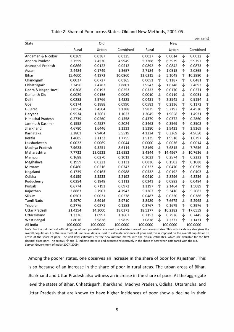
Table 2: Share of Poor across States: Old and New Methods, 2004-05

(per cent)

State Old New

Rural Urban Combined Rural Urban Combined

Andaman & Nicobar 0.0269

0.0387

0.0325

0.0027 ↓ 0.0014 ↓ 0.0022 ↓ Andhra Pradesh 2.7559

7.4570

4.9949

5.7268 ↑ 6.3939 ↓ 5.9797 ↑

Arunachal Pradesh 0.0866

0.0122

0.0512

0.0892 ↑ 0.0842 ↑ 0.0873 ↑ Assam 2.4484

0.1749

1.3657

2.7184 ↑ 1.0515 ↑ 2.0865 ↑

Bihar 15.4600

4.1972

10.0960

13.6315 ↓ 5.1048 ↑ 10.3990 ↓ Chandigarh 0.0037

0.0727

0.0365

0.0051 ↑ 0.1187 ↑ 0.0481 ↑

Chhattisgarh 3.2456

2.4782

2.8801

2.9543 ↓ 1.6748 ↓ 2.4693 ↓ Dadra & Nagar Haveli 0.0308

0.0193

0.0253

0.0333 ↑ 0.0170 ↓ 0.0271 ↑

Daman & Diu 0.0029

0.0156

0.0089

0.0010 ↓ 0.0119 ↓ 0.0051 ↓ Delhi 0.0283

2.9766

1.4325

0.0431 ↑ 2.3545 ↓ 0.9194 ↓

Goa 0.0174

0.1888

0.0990

0.0583 ↑ 0.2136 ↑ 0.1172 ↑ Gujarat 2.8554

3.4504

3.1388

3.9835 ↑ 5.2192 ↑ 4.4520 ↑

Haryana 0.9534

1.2661

1.1023

1.2045 ↑ 1.9658 ↑ 1.4931 ↑ Himachal Pradesh 0.2739

0.0260

0.1558

0.4379 ↑ 0.0372 ↑ 0.2860 ↑

Jammu & Kashmir 0.1558

0.2537

0.2024

0.3463 ↑ 0.3569 ↑ 0.3503 ↑ Jharkhand 4.6780

1.6446

3.2333

3.5280 ↓ 1.9423 ↑ 2.9269 ↓

Karnataka 3.3801

7.9404

5.5519

4.1334 ↑ 6.3269 ↓ 4.9650 ↓ Kerala 1.4685

2.1132

1.7755

1.5135 ↑ 1.9518 ↓ 1.6797 ↓

Lakshadweep 0.0022

0.0069

0.0044

0.0000 ↓ 0.0036 ↓ 0.0014 ↓ Madhya Pradesh 7.9623

9.3251

8.6114

7.8169 ↓ 7.6815 ↓ 7.7656 ↓

Maharashtra 7.7732

18.0933

12.6882

8.4844 ↑ 14.4967 ↓ 10.7636 ↓ Manipur 0.1688

0.0270

0.1013

0.2023 ↑ 0.2574 ↑ 0.2232 ↑

Meghalaya 0.1959

0.0221

0.1131

0.0836 ↓ 0.1502 ↑ 0.1088 ↓ Mizoram 0.0460

0.0216

0.0343

0.0323 ↓ 0.0470 ↑ 0.0379 ↑

Nagaland 0.1739

0.0163

0.0988

0.0532 ↓ 0.0192 ↑ 0.0403 ↓ Odisha 6.9159

3.3533

5.2192

6.0410 ↓ 2.8296 ↓ 4.8236 ↓

Puducherry 0.0354

0.1948

0.1113

0.0241 ↓ 0.0883 ↓ 0.0484 ↓ Punjab 0.6774

0.7191

0.6972

1.1197 ↑ 2.1464 ↑ 1.5089 ↑

Rajasthan 3.8883

5.7907

4.7943

5.1267 ↑ 5.3416 ↓ 5.2082 ↑ Sikkim 0.0503

0.0031

0.0278

0.0487 ↓ 0.0220 ↑ 0.0386 ↑

Tamil Nadu 3.4970

8.6916

5.9710

3.8489 ↑ 7.6675 ↓ 5.2965 ↓ Tripura 0.2776

0.0271

0.1583

0.3767 ↑ 0.1679 ↑ 0.2976 ↑

Uttar Pradesh 21.4354

14.3000

18.0371

18.5277 ↓ 16.2282 ↑ 17.6559 ↓ Uttarakhand 1.2276

1.0997

1.1667

0.7152 ↓ 0.7926 ↓ 0.7445 ↓

West Bengal 7.8016

3.9828

5.9829

7.0878 ↓ 7.2337 ↑ 7.1431 ↑ All India 100.0000

100.0000

100.0000

100.0000

100.0000

100.0000

Note: For the old method, official figures of poor population are used to calculate share of poor across states. This with incidence also gives the overall population. For the new method, unit level data is used to calculate incidence of poor and this is imposed on the overall population to arrive at the share of poor. The unit level estimates for the new method match with the official estimates, which are available for the first decimal place only. The arrows, ↑ and ↓ indicate increase and decrease respectively in the share of new when compared with the old. Source: Government of India (2007, 2009).

Among the poorer states, one observes an increase in the share of poor for Rajasthan. This

is so because of an increase in the share of poor in rural areas. The urban areas of Bihar,

Jharkhand and Uttar Pradesh also witness an increase in the share of poor. At the aggregate

level the states of Bihar, Chhattisgarh, Jharkhand, Madhya Pradesh, Odisha, Uttaranchal and

Uttar Pradesh that are known to have higher incidences of poor show a decline in their

10

share of poor. These will have important public policy implications on welfare related

interventions that are assigned on the basis of the share of poor.

4. Poverty and Inequality across States

Now we take up a discussion on poverty and of inequality across states of India. The poverty

measures are computed in the old as also new methods using Foster, Greer and Thorbecke

(1984; hereafter FGT) class of measures,

𝐹𝐺𝑇(∝) = 1 𝑁 ((𝑧 − 𝑌𝑖)/𝑧)∝; ∝≥ 0

𝑁

𝑖

where FGTα is the alpha class of poverty measure, N is total population, z is the poverty line,

yi is the consumption expenditure for the ith poor and α is a ‘poverty aversion’ parameter

(larger α gives greater weights to poorer people). This measure can be decomposed at

population sub-group level as

𝐹𝐺𝑇 ∝ = 𝑁𝑘

𝑁

𝐾

𝑘=1

𝐹𝐺𝑇 ∝ 𝑘 ; ∝≥ 0

where 𝑁𝑘

𝑁 is the number of persons in the subgroup 𝑘 divided by the total number of

persons, the subgroup population share.

The state-specific population poverty lines for the old and new methods are given in Table

3. The measures of incidence, depth and severity for poverty and inequality measured

through Gini coefficient for rural and urban areas across states are computed and given in

Table 4. State-specific broad shifts in incidence of poverty are also indicated through maps

in Figures 1 and 2 for rural and urban areas respectively.

Figure 3 has four graphs – two TIP (three I’s of poverty, see Jenkins and Lambert, 1997) and

two Lorenz curves for rural and urban areas. The TIP curves indicate incidence, intensity

(depth) and inequality among the poor (severity) and the Lorenz curves are a graphical

representation of the Gini coefficient. In each of the four graphs the old and new methods

are plotted separately. Comparing the new measures of poverty and inequality with that of

the old, some broad observations are as follows. We begin with the rural areas.

11

Table 3: Population and Poverty Lines for States, 2004-05

State Population (Lakhs) Poverty Line (`)

Rural Urban Rural Urban

Old New Old New

Andaman & Nicobar Islands

2.63 1.42 - 441.69 - 559.77 Andhra Pradesh 579.17 219.35 292.95 433.43 542.89 563.16 Arunachal Pradesh 8.68 2.87 - 547.14 - 618.45 Assam

244.02 38.71 387.64 478.00 378.84 600.03

Bihar 799.05 93.59 354.36 433.43 435.00 526.18 Chandigarh

1.07 9.43 - 642.51 - 642.51

Chhattisgarh 175.22 47.29 322.41 398.92 560.00 513.70 Dadra & Nagar Haveli

1.71 0.81 362.25 484.89 665.90 631.85

Daman & Diu

1.39 0.66 - 608.76 - 671.15 Delhi 9.05 146.64 410.38 541.39 612.91 642.47 Goa 6.78 7.71 362.25 608.76 665.90 671.15 Gujarat 332.76 208.64 353.93 501.58 541.16 659.18 Haryana 158.44 70.39 414.76 529.42 504.49 626.41 Himachal Pradesh 57.27 6.56 394.28 520.40 504.49 605.74 Jammu & Kashmir 80.22 27.61 391.26 522.30 553.77 602.89 Jharkhand 223.1 65.36 366.56 404.79 451.24 531.35 Karnataka 359.98 195.99 324.17 417.84 599.66 588.06 Kerala 244.81 85.08 430.12 537.31 559.39 584.70 Lakshadweep

0.42 0.28 - 537.31 - 584.70

Madhya Pradesh 476.35 175.67 327.78 408.41 570.15 532.26 Maharashtra 578.59 453.59 362.25 484.89 665.90 631.85 Manipur

16.82 5.98 - 578.11 - 641.13

Meghalaya

19.52 4.88 - 503.32 - 745.73 Mizoram

4.58 4.77 - 639.27 - 699.75

Nagaland

17.33 3.61 - 687.30 - 782.93 Odisha 324.55 60.35 325.79 407.78 528.49 497.31 Puducherry

3.43 7.14 - 384.45 - 506.17

Punjab 165.26 91.98 410.38 543.51 466.16 642.51 Rajasthan 467.13 144.23 374.57 478.00 559.63 568.15 Sikkim

5.01 0.68 - 531.50 - 741.68

Tamil Nadu 334.83 311.40 351.86 441.69 547.42 559.77 Tripura

27.67 5.99 - 450.49 - 555.70

Uttar Pradesh 1416.26 381.98 365.84 435.14 483.26 532.12 Uttarakhand 66.48 24.25 478.02 486.24 637.67 602.39 West Bengal 605.33 237.44 382.82 445.38 449.32 572.51 All India 7814.91 3142.33 356.30 446.68 538.60 578.80 Note: Population totals are rounded up at two decimals. The above population has been used for computations in Table 2. It has not been used in our other calculations using unit level data. Source: Government of India (2007, 2009)

The states of Meghalaya, Nagaland and Uttarakhand indicate a decline in the incidence of

poverty. The former two did not have a poverty line of their own as in the old method the

poverty ratio of Assam was used. One also observes a decline in the incidence of poverty in

the union territories of Andaman & Nicobar Islands, Daman & Diu and Lakshadweep. These

used the poverty ratio of their neighbouring states in the old method and in the new

method the incidences are independently computed by using the poverty lines of the

neighbouring states.

12

The maximum increase is for Goa (398 per cent; from 5.64 per cent to 28.09 per cent). It is

to be noted that the old method used the poverty line of Maharashtra whereas the new

method has a state-specific poverty line.

Increase in incidence of poverty is relatively higher for well-performing states (that is, those

with higher per capita gross state domestic product, GSDP). For instance, head count ratio

of poor in Punjab increases from 9 per cent in the old method to 22 per cent in the new

method, a 13 percentage point increase. The correlation coefficient between the Per Capita

Gross Domestic Product of major states and the percentage change in their rural poverty

line is 0.5828 and it is significant at one per cent level.

As indicated earlier, the four states with the maximum share of rural poor in the old method

(Uttar Pradesh, Bihar, Madhya Pradesh and West Bengal) have a reduction in their share of

rural poor in the new method. The share of Maharashtra, the fifth largest in the old

methodology, has increased and it has the third largest share in the new method.

Now, we take up some observations on urban areas. In the urban case as the incidence in

poverty in the old method was a starting point the changes at the aggregate level will cancel

out. In some states, it will increase and in the rest it will decrease.

In the states of Chhattisgarh, Karnataka, Madhya Pradesh, Maharashtra, Odisha and

Uttarakhand the urban poverty line in the new method is lower than that in the old method.

Needless to say, these are also the states where incidence of poverty has also declined. The

other major states where incidence of urban poverty has declined are Andhra Pradesh,

Kerala, Rajasthan and Tamil Nadu. The major states where urban poverty seems to have

increased are Assam, Bihar, Gujarat, Haryana, Himachal Pradesh, Jammu & Kashmir and

Uttar Pradesh among others. As indicated earlier, these will have implications on allocation

of resources for various welfare schemes, given a budget constraint.

13

Table 4: Poverty and Inequality across States with Old and New Methods, 2004-05, Rural and Urban

State Rural Urban

Poverty Inequality Poverty Inequality

Old Method New Method Old New Old Method New Method Old New

α = 0 α = 1 α = 2 α = 0 α = 1 α = 2 α = 0 α = 1 α = 2 α = 0 α = 1 α = 2 Andaman & Nicobar Is 22.49 3.23 0.79 3.29 0.22 0.02 0.3360 0.3081 21.96 3.68 0.88 0.81 0.01 0.00 0.3756 0.3430 Andhra Pradesh 10.47 1.95 0.68 32.29 6.97 2.27 0.2938 0.2677 27.36 5.74 1.80 23.37 4.81 1.49 0.3748 0.3627 Arunachal Pradesh 21.97 4.31 1.33 33.55 7.41 2.45 0.2800 0.2619 3.43 0.46 0.11 23.53 4.64 1.25 0.2480 0.2351 Assam 22.09 3.65 0.93 36.38 7.03 2.01 0.1986 0.1924 3.64 0.45 0.10 21.78 4.23 1.14 0.3201 0.3095 Bihar 42.59 8.14 2.21 55.71 12.68 3.91 0.2077 0.1943 36.09 7.43 2.23 43.73 11.43 3.86 0.3330 0.3201 Chandigarh 7.54 0.00 0.00 29.44 6.70 2.40 0.2465 0.2562 6.20 1.09 0.28 10.09 2.24 0.67 0.3608 0.3659 Chhattisgarh 40.77 9.24 3.14 55.06 13.69 4.92 0.2982 0.2644 42.18 12.30 4.79 28.39 7.20 2.58 0.4392 0.3717 Dadra & Nagar Haveli 39.64 8.50 3.33 63.63 18.02 7.14 0.3532 0.3345 19.17 6.24 2.26 16.81 4.98 1.63 0.3003 0.3087 Daman & Diu 4.53 0.75 0.23 2.41 0.47 0.09 0.2630 0.2518 19.06 3.63 0.85 14.43 2.08 0.32 0.2524 0.2382 Delhi 6.89 0.31 0.01 15.57 1.93 0.35 0.2779 0.2965 16.34 2.62 0.71 12.87 1.99 0.53 0.3362 0.3343 Goa 5.64 0.34 0.05 28.09 5.56 1.66 0.3213 0.2984 19.71 4.64 1.80 22.21 4.30 1.54 0.4195 0.3568 Gujarat 18.89 3.35 0.92 39.09 9.34 3.16 0.2731 0.2662 13.31 2.37 0.65 20.05 3.92 1.15 0.3098 0.3125 Haryana 13.25 2.34 0.64 24.82 4.73 1.33 0.3396 0.3261 14.48 3.26 1.06 22.39 4.93 1.62 0.3656 0.3414 Himachal Pradesh 10.53 1.60 0.38 24.97 4.22 1.12 0.3096 0.2893 3.19 0.86 0.33 4.55 1.07 0.41 0.3231 0.2803 Jammu & Kashmir 4.27 0.64 0.15 14.10 2.11 0.52 0.2473 0.2168 7.40 1.71 0.49 10.36 2.12 0.56 0.2476 0.2528 Jharkhand 46.15 9.88 2.94 51.64 11.12 3.37 0.2275 0.2086 20.25 4.29 1.31 23.82 5.77 1.90 0.3552 0.3360 Karnataka 20.67 2.86 0.64 37.49 6.51 1.67 0.2663 0.2457 32.61 8.73 3.25 25.88 6.19 2.13 0.3685 0.3687 Kerala 13.20 2.76 0.97 20.19 4.37 1.47 0.3809 0.3469 19.99 4.55 1.56 18.39 4.04 1.33 0.4102 0.3956 Lakshadweep 11.43 0.13 0.04 0.34 0.10 0.03 0.3115 0.2532 19.95 5.75 2.84 10.31 3.76 1.83 0.3939 0.2647 Madhya Pradesh 36.79 8.01 2.52 53.59 12.57 4.16 0.2675 0.2518 42.72 12.07 4.62 35.05 8.59 2.93 0.3980 0.3676 Maharashtra 29.57 6.31 1.99 47.54 11.87 4.23 0.3120 0.2874 32.10 9.13 3.56 25.62 6.48 2.29 0.3776 0.3688 Manipur 22.01 2.92 0.57 39.28 5.71 1.26 0.1602 0.1523 3.59 0.28 0.04 34.51 5.12 1.03 0.1774 0.1650 Meghalaya 21.95 2.69 0.52 13.98 1.40 0.23 0.1618 0.1497 3.62 0.34 0.06 24.68 2.80 0.53 0.2635 0.2612 Mizoram 22.09 3.27 0.83 23.04 3.49 0.89 0.2010 0.1856 3.62 0.37 0.07 7.89 1.00 0.22 0.2490 0.2291 Nagaland 22.05 2.79 0.55 10.02 1.02 0.19 0.2293 0.2056 3.30 0.24 0.03 4.26 0.54 0.10 0.2422 0.2336 Odisha 46.91 12.11 4.33 60.78 17.37 6.63 0.2852 0.2659 44.72 13.40 5.41 37.59 9.60 3.50 0.3535 0.3402 Puducherry 22.69 2.44 0.37 22.91 3.99 0.84 0.3471 0.3263 21.96 3.65 0.92 9.92 1.33 0.29 0.3156 0.3202 Punjab 9.02 1.19 0.26 22.12 3.76 0.97 0.2942 0.2854 6.29 0.67 0.12 18.71 3.17 0.77 0.4021 0.3378 Rajasthan 18.32 2.96 0.74 35.84 7.01 2.00 0.2496 0.2213 32.31 7.18 2.30 29.69 5.75 1.68 0.3715 0.3222 Sikkim 22.07 3.47 0.76 31.77 5.62 1.43 0.2728 0.2539 3.44 0.71 0.25 25.95 3.35 0.89 0.2561 0.2447 Tamil Nadu 22.99 3.80 1.00 37.54 7.43 2.13 0.3222 0.2758 22.46 4.70 1.46 19.74 4.09 1.25 0.3609 0.3644 Tripura 22.08 3.38 0.84 44.46 9.58 2.90 0.2185 0.2114 3.47 0.43 0.09 22.47 3.80 0.96 0.3415 0.3134 Uttar Pradesh 33.32 6.33 1.81 42.72 9.16 2.77 0.2902 0.2524 30.13 7.05 2.34 34.06 7.80 2.53 0.3691 0.3545 Uttarakhand 40.65 7.77 2.11 35.13 5.80 1.41 0.2851 0.2394 36.50 8.47 2.59 26.20 5.09 1.41 0.3268 0.3163 West Bengal 28.37 5.31 1.46 38.23 7.92 2.35 0.2738 0.2555 13.50 2.48 0.68 24.42 5.29 1.64 0.3833 0.3725 All India 28.12 5.50 1.63 41.80 9.24 2.94 0.3045 0.2808 25.84 6.21 2.16 25.68 5.78 1.88 0.3764 0.3643

Note: Calculations use poverty lines and assumptions given in official publications (see Table 3 and note in Table 1), but the state-specific incidences do not match, particularly for the old method. Source: Unit level data, Schedule 1.0, NSS 61

st Round, 2004-05.

14

Figure 1: Map Depicting Incidence of Poor across States in Rural India, 2004-05 (a) Old Method and (b) New Method

15

Figure 2: Map Depicting Incidence of Poor across States in Urban India, 2004-05 (a) Old Method and (b) New Method

16

Figure 3: TIP and Lorenz Curves for India with Old and New Methods, 2004-05, Rural and Urban

17

5. Poverty and Inequality across Sub-groups of Population

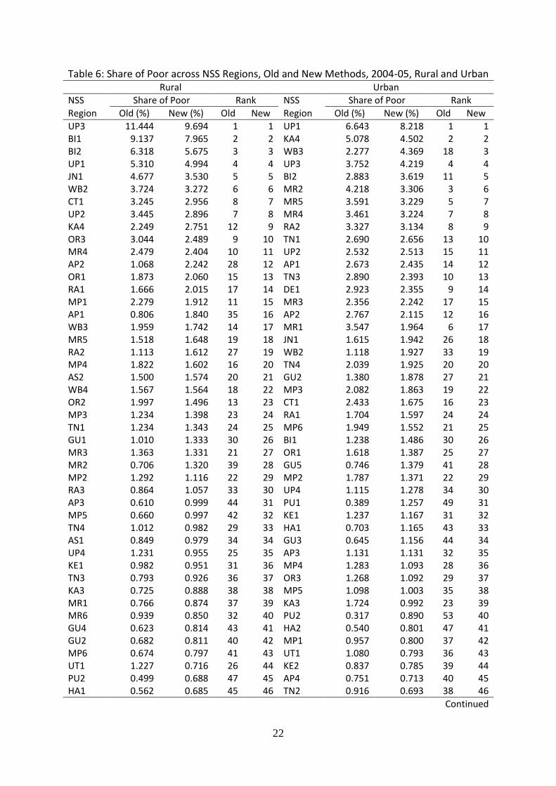
5.1 NSS Regions

The poorest two NSS regions of rural India in 2004-05 are southern and northern Odisha

(headcount ratio or HCR of 81 per cent and 72 per cent respectively), see Table 5. The two

regions together include the undivided districts of Koraput, Bolangir and Kalahandi (the KBK

districts that have received public policy and media attention for hunger and starvation

deaths), and Kandhamal that came into discussion because of communal strife in recent

years. They also are the mineral and resource-rich areas with a greater concentration of the

tribal population. The remaining region from Odisha comprising the coastal districts also has

incidence of poor which is greater than the all India average, which is 41.7 per cent, under

the new method. For a discussion on poverty scenario in Odisha see Mishra (2009b).

Further, in the new method, there are 30 more rural regions where the incidence of poverty

is greater than two-fifths. They include the hills region (one of the three) from Assam, the

south western and inland southern regions (two of the four) from Andhra Pradesh, both the

regions from Bihar, Chhattisgarh, Dadra & Nagar Haveli, the eastern and dry areas regions

(two of the five) from Gujarat, Jharkhand, the inland northern region (one of the four) from

Karnataka, all the six regions from Madhya Pradesh, five of the six regions from

Maharashtra (it excludes western Maharashtra region only), the hills region (one of the two)

from Manipur, the southern and western regions (two of the four) from Rajasthan, the

coastal northern region (one of the four) from Tamil Nadu, Tripura, eastern and southern

regions (two of the four) from Uttar Pradesh, and eastern plains region (one of the four)

from West Bengal.

When it comes to the share of poor across regions, it is eastern region of Uttar Pradesh that

stands out (Table 6).6 Under the new method, it accounts for nearly 10 per cent of the

country's rural poor. The two regions of Bihar, the northern region of Uttar Pradesh and

Jharkhand account for another 22 per cent of the rural poor. The eastern plains region of

West Bengal, Chhattisgarh, central region of Uttar Pradesh, inland northern region of

6 For a discussion on poverty scenario in Uttar Pradesh see Pathak (2010).

18

Karnataka, and northern region of Odisha account for another 14 per cent of the rural poor.

This means that ten regions account for 46 per cent share of the rural poor.

In urban areas, inland central region of Maharashtra has the highest incidence of poor.7

Under the new method, it is 61 per cent. The hills region of Manipur has 51 per cent

incidence of poverty. Eleven more regions (inland northern Karnataka, southern Uttar

Pradesh, southern Odisha, inland northern Maharashtra, eastern plains of West Bengal,

northern Madhya Pradesh, central Bihar, eastern Uttar Pradesh, inland eastern Maharashtra

and south western Andhra Pradesh) have poverty incidence greater than two-fifths.

Including all these, a total of 38 regions have poverty incidence greater than 25 per cent.

With regard to share of poor in urban areas, western Uttar Pradesh has the highest share. In

the new method it is 8 per cent. This along with inland northern of Karnataka, central plains

of West Bengal, eastern Uttar Pradesh and central Bihar account for 25 per cent share of

urban poor. Inland western, inland eastern and inland central regions of Maharashtra

accounting for ten per cent of the urban poor, which increases to more than 18 per cent if

we include the other three regions of Maharashtra.

7 For a discussion on socio-economic inequities and calorie deprivation in Maharashtra see Mishra (2009a) and

Mishra and Hari (2009) respectively.

19

Table 5: Poverty and Inequality across NSS Regions with Old and New Methods, 2004-05, Rural and Urban Rural Urban

NSS Poverty Inequality NSS Poverty Inequality

Region Old Method New Method Old New Region Old Method New Method Old New

α = 0 α = 1 α = 2 α = 0 α = 1 α = 2 α = 0 α = 1 α = 2 α = 0 α = 1 α = 2

AN1 22.49 3.23 0.79 3.29 0.22 0.02 0.3360 0.3081 AN1 21.96 3.68 0.88 0.81 0.01 0.00 0.3756 0.3430 AP1 6.97 1.53 0.63 23.58 5.26 1.85 0.2826 0.2624 AP1 21.93 4.57 1.49 19.53 4.03 1.29 0.3778 0.3517 AP2 11.05 1.66 0.49 34.38 6.73 1.98 0.2931 0.2611 AP2 28.19 5.48 1.57 21.07 3.96 1.06 0.3854 0.3811 AP3 22.44 4.38 1.44 54.45 12.78 4.27 0.2697 0.2443 AP3 41.34 10.18 3.56 40.45 9.21 3.09 0.3252 0.3335 AP4 11.52 2.37 0.81 40.87 9.68 3.26 0.3155 0.2863 AP4 37.20 8.11 2.42 34.52 7.74 2.61 0.2885 0.3234 AR1 21.97 4.31 1.33 33.55 7.41 2.45 0.2800 0.2619 AR1 3.43 0.46 0.11 23.53 4.64 1.25 0.2480 0.2351 AS1 20.74 3.14 0.70 35.45 6.55 1.71 0.2089 0.2001 AS1 4.01 0.45 0.08 21.15 4.55 1.26 0.3601 0.3141 AS2 22.85 4.04 1.11 35.55 7.32 2.23 0.1927 0.1886 AS2 3.53 0.48 0.12 21.23 3.95 1.08 0.2919 0.3068 AS3 23.24 2.48 0.43 58.12 7.21 1.38 0.1216 0.1182 AS3 1.43 0.06 0.00 36.69 5.37 1.00 0.2091 0.2137 BI1 41.60 7.80 2.09 53.74 12.21 3.77 0.2134 0.1987 BI1 38.60 9.43 3.01 45.32 12.96 4.72 0.3064 0.3059 BI2 44.11 8.67 2.41 58.72 13.39 4.13 0.1972 0.1859 BI2 35.12 6.64 1.93 43.10 10.83 3.52 0.3405 0.3241 CN1 7.54 0.00 0.00 15.47 3.74 1.29 0.2465 0.2562 CN1 6.20 1.09 0.28 10.09 2.24 0.67 0.3608 0.3659 CT1 40.77 9.24 3.14 55.06 13.69 4.92 0.2982 0.2644 CT1 34.62 10.64 4.08 28.39 7.20 2.58 0.4392 0.3717 DA1 39.64 8.50 3.33 63.63 18.02 7.14 0.3532 0.3345 DA1 19.17 6.24 2.26 16.81 4.98 1.63 0.3003 0.3087 DD1 4.53 0.75 0.23 2.41 0.47 0.09 0.2630 0.2518 DD1 19.06 3.63 0.85 14.43 2.08 0.32 0.2524 0.2382 DE1 6.89 0.31 0.01 15.57 1.93 0.35 0.2779 0.2965 DE1 16.34 2.62 0.71 12.87 1.99 0.53 0.3362 0.3343 GO1 5.64 0.34 0.05 28.09 5.56 1.66 0.3213 0.2984 GO1 19.71 4.64 1.80 22.21 4.30 1.54 0.4195 0.3568 GU1 26.15 4.85 1.49 51.18 13.23 4.63 0.2704 0.2672 GU1 15.64 2.99 0.99 24.94 5.08 1.61 0.2768 0.3038 GU2 21.57 3.28 0.76 38.03 9.47 3.08 0.2893 0.2967 GU2 16.48 3.06 0.79 21.93 4.76 1.41 0.3442 0.3436 GU3 17.93 3.18 0.81 39.79 9.31 3.01 0.3075 0.2861 GU3 8.04 1.43 0.42 14.08 2.55 0.71 0.2996 0.3085 GU4 24.97 4.94 1.42 48.34 11.63 4.28 0.2159 0.2236 GU4 28.49 4.90 1.50 27.47 6.59 2.17 0.2535 0.2662 GU5 2.71 0.37 0.06 16.70 2.43 0.57 0.2181 0.2041 GU5 12.45 2.02 0.52 22.50 3.72 1.02 0.2496 0.2321 HA1 12.69 2.12 0.54 22.95 4.36 1.20 0.3617 0.3612 HA1 11.21 2.78 0.98 18.16 3.93 1.40 0.3560 0.3464 HA2 14.14 2.69 0.78 27.81 5.32 1.53 0.2873 0.2394 HA2 23.32 4.57 1.26 33.86 7.63 2.22 0.3785 0.2888 HP1 10.53 1.60 0.38 24.97 4.22 1.12 0.3096 0.2893 HP1 3.19 0.86 0.33 4.55 1.07 0.41 0.3231 0.2803 JK1 2.93 0.32 0.05 4.97 0.95 0.25 0.2552 0.2275 JK1 4.13 0.98 0.31 4.65 0.90 0.26 0.2667 0.2736 JK2 9.26 1.64 0.51 32.72 4.39 1.03 0.1465 0.1510 JK2 3.95 0.56 0.12 9.26 1.04 0.18 0.1876 0.2112 JK3 3.96 0.59 0.13 14.63 2.19 0.54 0.2382 0.2025 JK3 9.20 2.14 0.60 13.19 2.78 0.73 0.2196 0.2147 JN1 46.15 9.88 2.94 51.64 11.12 3.37 0.2275 0.2086 JN1 20.25 4.29 1.31 23.82 5.77 1.90 0.3552 0.3360

Continued

20




α = 0 α = 1 α = 2 α = 0 α = 1 α = 2 α = 0 α = 1 α = 2 α = 0 α = 1 α = 2

KA1 20.26 3.04 0.75 26.98 6.43 2.04 0.3821 0.3151 KA1 42.88 12.03 4.07 38.16 8.57 2.55 0.4453 0.4281 KA2 5.10 0.55 0.07 17.81 2.00 0.38 0.2313 0.2211 KA2 28.96 5.34 1.38 20.49 3.16 0.76 0.2743 0.2800 KA3 15.15 1.72 0.35 27.47 3.98 0.90 0.2540 0.2484 KA3 14.07 2.71 0.84 7.91 1.50 0.45 0.3335 0.3391 KA4 27.35 4.00 0.90 49.60 8.97 2.33 0.2296 0.2036 KA4 57.04 17.01 6.71 49.47 12.73 4.58 0.3238 0.3049 KE1 21.12 4.31 1.47 30.31 6.76 2.30 0.3550 0.3138 KE1 33.49 8.94 3.33 30.88 8.08 2.94 0.4235 0.3813 KE2 7.51 1.63 0.61 12.91 2.65 0.88 0.3759 0.3458 KE2 12.53 2.13 0.58 11.49 1.81 0.44 0.3888 0.3841 LA1 11.43 0.13 0.04 0.34 0.10 0.03 0.3115 0.2532 LA1 19.95 5.75 2.84 10.31 3.76 1.83 0.3939 0.2647 MP1 48.02 11.11 3.44 59.72 14.22 4.51 0.2508 0.2361 MP1 48.83 14.85 6.30 28.29 7.18 2.44 0.3093 0.3050 MP2 50.40 12.11 4.17 64.53 17.67 6.62 0.2521 0.2460 MP2 32.62 9.47 3.52 36.63 10.45 4.08 0.3284 0.3445 MP3 25.09 5.12 1.67 42.10 9.41 3.10 0.3029 0.2886 MP3 47.55 12.81 4.91 28.55 6.81 2.18 0.4615 0.4017 MP4 49.45 11.56 3.71 64.46 16.91 6.04 0.2522 0.2312 MP4 43.65 11.05 3.65 39.62 9.03 3.10 0.3380 0.3075 MP5 23.78 3.98 1.05 53.22 10.46 2.93 0.2120 0.2032 MP5 57.14 15.31 5.78 38.99 8.54 2.50 0.3321 0.3195 MP6 22.87 3.64 0.92 40.10 7.34 2.06 0.2185 0.2128 MP6 34.62 10.64 4.08 44.50 10.77 3.66 0.3632 0.3298 MR1 26.03 5.71 1.88 44.03 11.49 4.36 0.3204 0.3151 MR1 14.51 2.75 0.78 7.86 1.36 0.35 0.3597 0.3394 MR2 9.55 1.24 0.27 26.47 3.95 0.95 0.2766 0.2606 MR2 36.81 8.92 3.02 28.22 5.77 1.68 0.3271 0.3418 MR3 37.94 8.74 3.06 54.91 15.29 6.00 0.2846 0.2676 MR3 48.17 15.30 6.54 44.84 12.80 5.18 0.3619 0.3478 MR4 42.64 9.72 3.05 61.30 16.39 5.88 0.3277 0.2668 MR4 66.17 25.03 11.19 60.29 18.37 7.08 0.3395 0.3295 MR5 33.45 6.14 1.62 53.81 12.93 4.19 0.2822 0.2623 MR5 46.88 14.74 5.96 41.22 11.31 4.10 0.3708 0.3604 MR6 47.05 12.03 4.41 63.13 19.96 8.26 0.3422 0.3265 MR6 35.77 10.53 4.27 31.44 8.34 3.23 0.2902 0.3026 MU1 13.02 1.50 0.27 24.53 3.02 0.58 0.1655 0.1529 MU1 3.17 0.23 0.03 33.55 4.78 0.93 0.1762 0.1627 MU2 32.60 4.59 0.92 56.65 8.87 2.05 0.1276 0.1248 MU2 10.91 1.16 0.16 51.36 11.05 2.88 0.1811 0.1944 MY1 21.95 2.69 0.52 13.98 1.40 0.23 0.1618 0.1497 MY1 3.62 0.34 0.06 24.68 2.80 0.53 0.2635 0.2612 MZ1 22.09 3.27 0.83 23.04 3.49 0.89 0.2010 0.1856 MZ1 3.62 0.37 0.07 7.89 1.00 0.22 0.2490 0.2291 NA1 22.05 2.79 0.55 10.02 1.02 0.19 0.2293 0.2056 NA1 3.30 0.24 0.03 4.26 0.54 0.10 0.2422 0.2336 OD1 27.39 5.34 1.55 44.64 9.52 2.98 0.2561 0.2311 OD1 44.11 12.27 4.72 36.99 8.90 3.08 0.3426 0.3382 OD2 72.66 24.31 10.04 80.70 30.32 13.67 0.2678 0.2612 OD2 55.03 19.73 9.19 46.39 15.11 6.46 0.4664 0.3915 OD3 59.07 14.58 4.98 71.58 20.88 7.72 0.2812 0.2700 OD3 42.90 13.22 5.32 36.12 9.10 3.28 0.3339 0.3281 PD1 22.69 2.44 0.37 22.91 3.99 0.84 0.3471 0.3263 PD1 21.96 3.65 0.92 9.92 1.33 0.29 0.3156 0.3202 PN1 4.37 0.51 0.08 15.66 2.12 0.44 0.2825 0.2799 PN1 5.11 0.51 0.08 16.16 2.40 0.54 0.4147 0.3310 PN2 14.60 2.00 0.47 29.87 5.71 1.61 0.3047 0.2835 PN2 8.78 1.02 0.21 24.07 4.80 1.24 0.3674 0.3473

Continued

21




α = 0 α = 1 α = 2 α = 0 α = 1 α = 2 α = 0 α = 1 α = 2 α = 0 α = 1 α = 2

RA1 22.52 3.89 1.03 40.38 8.22 2.44 0.2655 0.2294 RA1 30.03 6.87 2.33 27.52 5.58 1.72 0.3122 0.3148 RA2 12.73 1.84 0.41 27.33 4.74 1.20 0.2369 0.2060 RA2 36.04 8.06 2.50 33.20 6.35 1.79 0.4082 0.3149 RA3 30.36 4.66 1.12 55.02 12.06 3.66 0.2551 0.2386 RA3 23.63 4.19 1.04 20.52 3.24 0.76 0.2978 0.2946 RA4 10.94 2.10 0.53 29.64 5.43 1.59 0.2109 0.2060 RA4 25.01 5.35 2.06 23.79 4.79 1.66 0.3721 0.3772 SI1 22.07 3.47 0.76 31.77 5.62 1.43 0.2728 0.2539 SI1 3.44 0.71 0.25 25.95 3.35 0.89 0.2561 0.2447 TN1 28.14 4.82 1.28 45.41 9.87 2.96 0.3069 0.2860 TN1 16.54 2.95 0.75 15.98 3.10 0.88 0.3719 0.3772 TN2 13.54 1.58 0.34 26.32 3.93 0.92 0.2875 0.2581 TN2 21.03 3.57 1.03 15.58 2.67 0.73 0.3078 0.3169 TN3 21.70 3.35 0.93 37.56 6.73 1.84 0.3094 0.2643 TN3 34.55 7.92 2.63 27.98 6.33 1.98 0.3068 0.3186 TN4 26.69 5.01 1.32 38.40 8.40 2.51 0.3737 0.2828 TN4 22.62 5.42 1.85 20.88 4.50 1.49 0.3609 0.3566 TR1 22.08 3.38 0.84 44.46 9.58 2.90 0.2185 0.2114 TR1 3.47 0.43 0.09 22.47 3.80 0.96 0.3415 0.3134 UP1 24.07 3.90 0.97 33.56 5.94 1.54 0.2873 0.2512 UP1 27.98 6.26 1.94 33.86 7.24 2.17 0.3508 0.3478 UP2 30.12 5.65 1.56 37.53 8.55 2.62 0.2950 0.2572 UP2 24.64 6.16 2.25 23.92 6.13 2.32 0.4238 0.3863 UP3 41.37 8.44 2.56 51.94 11.82 3.76 0.2750 0.2366 UP3 37.53 8.55 2.74 41.27 9.58 3.03 0.3203 0.3090 UP4 38.87 7.33 2.02 44.69 10.64 3.32 0.3111 0.2609 UP4 43.01 12.03 4.82 48.22 12.70 4.73 0.3084 0.2659 UT1 40.65 7.77 2.11 35.13 5.80 1.41 0.2851 0.2394 UT1 36.50 8.47 2.59 26.20 5.09 1.41 0.3268 0.3163 WB1 20.09 3.52 1.00 27.78 5.09 1.47 0.2267 0.2027 WB1 15.40 2.10 0.48 32.50 7.08 1.94 0.3149 0.3064 WB2 42.88 8.51 2.36 55.85 12.58 3.77 0.2635 0.2367 WB2 26.45 5.52 1.53 44.59 11.06 3.70 0.3541 0.3487 WB3 20.06 2.91 0.68 26.45 4.33 1.10 0.2546 0.2452 WB3 10.55 1.84 0.50 19.79 3.96 1.18 0.3867 0.3753 WB4 24.85 5.39 1.63 36.76 8.30 2.73 0.3102 0.2795 WB4 17.05 3.23 0.91 26.86 6.34 2.16 0.3060 0.2954 AI 28.12 5.50 1.63 41.80 9.24 2.94 0.3045 0.2808 AI 25.84 6.21 2.16 25.68 5.78 1.88 0.3764 0.3643 Note: The first two letter codes refer to the state as follows: AI=All India, AN=Andaman & Nicobar Islands, AP=Andhra Pradesh, AR=Arunachal Pradesh, AS=Assam, BI=Bihar, CN=Chandigarh, CT=Chhattisgarh, DA=Dadra & Nagar Haveli, DD=Daman & Diu, DE=Delhi, GO=Goa, GU=Gujarat, HA=Haryana, HP=Himachal Pradesh, JK=Jammu & Kashmir, JN=Jharkhand, KA=Karnataka, KE=Kerala, LA=Lakshadweep, MP=Madhya Pradesh, MR=Maharashtra, MU=Manipur, MY=Meghalaya, MZ=Mizoran, NA=Nagaland, OD=Odisha, PD=Puducherry, PN=Punjab, RA=Rajasthan, SI=Sikkim, TN=Tamil Nadu, TR=Tripura, UP=Uttar Pradesh, UT=Uttarakhand, and WB=West Bengal. And the number refers to the region within the state. In those states with more than one region they refer to the following: AP1=Coastal, AP2=Inland Northern, AP3=South Western, AP4=Inland Southern, AS1=Plains Eastern, AS2=Plains Western, AS3=Hills, BI1=Northern, BI2=Central, GU1=Eastern, GU2=Plains Northern, GU3=Plains Southern, GU4=Dry Areas, GU5=Saurashtra, HA1=Eastern, HA2=Western, JK1=Mountainous, JK2=Outer Hills, JK3=Jhelam Valley, KA1=Coastal & Ghats, KA2=Inland Eastern, KA3=Inland Southern, KA4=Inland Northern, KE1=Northern, KE2=Southern, MP1=Vindhya, MP2=Central, MP3=Malwa, MP4=South, MP5=South Western, MP6=Northern, MR1=Coastal, MR2=Inland Western, MR3=Inland Northern, MR4=Inland Central, MR5=Inland Eastern, MR6=Eastern, MU1=Plains, MU2=Hills, OD1=Coastal, OD2=Southern, OD3=Northern, PN1=Northern, PN2=Southern, RA1=Western, RA2=North Eastern, RA3=Southern, RA4=South Eastern, TN1=Coastal Northern, TN2=Coastal, TN3=Southern, TN4=Inland, UP1=Western, UP2=Central, UP3=Eastern, UP4=Southern, WB1=Himalayan, WB2=Eastern Plains, WB3=Central Plains and WB4=Western Plains. AI refers to All-India. In the old method, there are no independent estimates for 12 smaller states/union territories; poverty ratio of a neighbouring reference state has been used. For details, see notes in Tables 1 and 4. Source: Unit level data, Schedule 1.0, NSS 61st Round, 2004-05.

22

Table 6: Share of Poor across NSS Regions, Old and New Methods, 2004-05, Rural and Urban

Rural Urban

NSS Share of Poor Rank NSS Share of Poor Rank

Region Old (%) New (%) Old New Region Old (%) New (%) Old New

UP3 11.444 9.694 1 1 UP1 6.643 8.218 1 1 BI1 9.137 7.965 2 2 KA4 5.078 4.502 2 2 BI2 6.318 5.675 3 3 WB3 2.277 4.369 18 3 UP1 5.310 4.994 4 4 UP3 3.752 4.219 4 4 JN1 4.677 3.530 5 5 BI2 2.883 3.619 11 5 WB2 3.724 3.272 6 6 MR2 4.218 3.306 3 6 CT1 3.245 2.956 8 7 MR5 3.591 3.229 5 7 UP2 3.445 2.896 7 8 MR4 3.461 3.224 7 8 KA4 2.249 2.751 12 9 RA2 3.327 3.134 8 9 OR3 3.044 2.489 9 10 TN1 2.690 2.656 13 10 MR4 2.479 2.404 10 11 UP2 2.532 2.513 15 11 AP2 1.068 2.242 28 12 AP1 2.673 2.435 14 12 OR1 1.873 2.060 15 13 TN3 2.890 2.393 10 13 RA1 1.666 2.015 17 14 DE1 2.923 2.355 9 14 MP1 2.279 1.912 11 15 MR3 2.356 2.242 17 15 AP1 0.806 1.840 35 16 AP2 2.767 2.115 12 16 WB3 1.959 1.742 14 17 MR1 3.547 1.964 6 17 MR5 1.518 1.648 19 18 JN1 1.615 1.942 26 18 RA2 1.113 1.612 27 19 WB2 1.118 1.927 33 19 MP4 1.822 1.602 16 20 TN4 2.039 1.925 20 20 AS2 1.500 1.574 20 21 GU2 1.380 1.878 27 21 WB4 1.567 1.564 18 22 MP3 2.082 1.863 19 22 OR2 1.997 1.496 13 23 CT1 2.433 1.675 16 23 MP3 1.234 1.398 23 24 RA1 1.704 1.597 24 24 TN1 1.234 1.343 24 25 MP6 1.949 1.552 21 25 GU1 1.010 1.333 30 26 BI1 1.238 1.486 30 26 MR3 1.363 1.331 21 27 OR1 1.618 1.387 25 27 MR2 0.706 1.320 39 28 GU5 0.746 1.379 41 28 MP2 1.292 1.116 22 29 MP2 1.787 1.371 22 29 RA3 0.864 1.057 33 30 UP4 1.115 1.278 34 30 AP3 0.610 0.999 44 31 PU1 0.389 1.257 49 31 MP5 0.660 0.997 42 32 KE1 1.237 1.167 31 32 TN4 1.012 0.982 29 33 HA1 0.703 1.165 43 33 AS1 0.849 0.979 34 34 GU3 0.645 1.156 44 34 UP4 1.231 0.955 25 35 AP3 1.131 1.131 32 35 KE1 0.982 0.951 31 36 MP4 1.283 1.093 28 36 TN3 0.793 0.926 36 37 OR3 1.268 1.092 29 37 KA3 0.725 0.888 38 38 MP5 1.098 1.003 35 38 MR1 0.766 0.874 37 39 KA3 1.724 0.992 23 39 MR6 0.939 0.850 32 40 PU2 0.317 0.890 53 40 GU4 0.623 0.814 43 41 HA2 0.540 0.801 47 41 GU2 0.682 0.811 40 42 MP1 0.957 0.800 37 42 MP6 0.674 0.797 41 43 UT1 1.080 0.793 36 43 UT1 1.227 0.716 26 44 KE2 0.837 0.785 39 44 PU2 0.499 0.688 47 45 AP4 0.751 0.713 40 45 HA1 0.562 0.685 45 46 TN2 0.916 0.693 38 46

Continued

23

Table 6: Share of Poor across NSS Regions, Old and New Methods, 2004-05, Rural and Urban

Rural Urban

NSS Share of Poor Rank NSS Share of Poor Rank

Region Old (%) New (%) Old New Region Old (%) New (%) Old New

GU3 0.457 0.685 49 47 AS2 0.096 0.592 67 47 AP4 0.271 0.649 55 48 KA1 0.609 0.554 45 48 TN2 0.457 0.600 50 49 MR6 0.593 0.533 46 49 KE2 0.486 0.563 48 50 WB4 0.320 0.515 52 50 HA2 0.392 0.520 51 51 GU1 0.309 0.503 54 51 WB1 0.550 0.513 46 52 WB1 0.196 0.422 63 52 RA4 0.244 0.446 56 53 AS1 0.073 0.394 68 53 HP1 0.274 0.438 54 54 OR2 0.407 0.351 48 54 PU1 0.179 0.432 58 55 RA4 0.348 0.339 51 55 TR1 0.278 0.377 53 56 GU4 0.308 0.303 55 56 GU5 0.082 0.343 65 57 JK3 0.200 0.293 61 57 KA1 0.314 0.282 52 58 KA2 0.386 0.279 50 58 JK3 0.090 0.225 63 59 RA3 0.307 0.272 56 59 KA2 0.091 0.215 62 60 MU1 0.251 0.237 58 60 AS3 0.099 0.166 60 61 GO1 0.185 0.214 64 61 MU2 0.077 0.134 66 62 TR1 0.266 0.168 57 62 JK2 0.038 0.089 69 63 MY1 0.217 0.150 59 63 AR1 0.087 0.089 64 64 CN1 0.724 0.119 42 64 MY1 0.196 0.084 57 65 PO1 0.196 0.088 62 65 MU1 0.091 0.068 61 66 AR1 0.127 0.084 66 66 GO1 0.017 0.058 76 67 AS3 0.003 0.066 78 67 NA1 0.174 0.053 59 68 JK1 0.043 0.050 69 68 SI1 0.050 0.049 67 69 MZ1 0.212 0.047 60 69 DE1 0.028 0.043 73 70 HP1 0.025 0.037 72 70 DA1 0.031 0.033 71 71 SI1 0.030 0.022 71 71 MZ1 0.046 0.032 68 72 MU2 0.014 0.021 75 72 JK1 0.028 0.032 74 73 NA1 0.160 0.019 65 73 PO1 0.036 0.024 70 74 DA1 0.019 0.017 73 74 CN1 0.031 0.005 72 75 JK2 0.006 0.014 77 75 AN1 0.027 0.003 75 76 DD1 0.016 0.012 74 76 DD1 0.004 0.001 77 77 LA1 0.007 0.004 76 77 LA1 0.003 0.000 78 78 AN1 0.039 0.001 70 78 Note: The NSS Region Codes are as in Table 5. Source Unit level data, Schedule 1.0, NSS 61

st Round, 2004-05.

24

5.2 Social Groups

The poorest social group is scheduled tribes from rural Orissa (Table 7). In the new method

their incidence of poverty is 84 per cent. The other vulnerable groups in rural areas are

scheduled tribes of Madhya Pradesh (80 per cent), scheduled castes of Bihar (77 per cent)

and scheduled tribes of Maharashtra (72 per cent). Besides these, there are nine more social

groups with incidence of poverty greater than 60 per cent under the new method. They are

the scheduled tribes of Andhra Pradesh, Bihar, Chhattisgarh, Dadra & Nagar Haveli and

Jharkhand and the scheduled castes of Jharkhand, Madhya Pradesh, Mizoram and Odisha. In

addition, seventeen more social groups have a poverty incidence greater than 50 per cent of

which eight are scheduled tribes, two are scheduled castes and seven are backward classes.

Another 21 social groups have incidence of poverty greater that 40 per cent, of which three

are scheduled tribes, ten are scheduled castes, six are backward classes and two are others.

Further, in rural areas under the new method scheduled tribes are the poorest groups in

twenty states/union territories. Scheduled castes are the poorest in thirteen states (Assam,

Bihar, Haryana, Himachal Pradesh, Jharkhand, Karnataka, Mizoram, Puducherry, Punjab,

Sikkim, Tamil Nadu, Uttar Pradesh and Uttarakhand).8 Backward classes are the poorest in

five (Arunachal Pradesh, Daman & Diu, Delhi, Goa and Nagaland) and other classes in two

(Andaman and Nicobar Island and Chandigarh), but one should be cautious while reading

the results for sub-groups in smaller states/union territories with lower sample size.

The poorest social group in urban areas is scheduled castes of Bihar with an incidence of

poverty of 71 per cent under the new method. Scheduled castes of Dadra & Nagar Haveli,

Goa, Madhya Pradesh and Odisha also indicate a poverty incidence of 60 per cent or more.

Another eight social groups indicate a poverty incidence greater than 50 per cent of which

eight are from among scheduled tribes (Andhra Pradesh, Bihar, Dadra & Nagar Haveli,

Karnataka and Odisha) and three from among scheduled castes (Jharkhand, Rajasthan and

Sikkim). With an incidence of poverty between 25 to 50 per cent there are another 24

states/union territories of which 11 are scheduled castes, five are scheduled tribes, seven

are backward classes and one is 'others'. Overall, in 23 states/union territories the

8 For a larger discussion on scheduled castes using earlier data sources see the papers and references therein

in a special issues of the Journal of Indian School of Political Economy (Betéille, 2000). A recent discourse on social exclusion is an edited book by Thorat and Newman (2009).

25

scheduled castes have the highest incidence of poverty, six are scheduled tribes (Andhra

Pradesh, Karnataka, Lakshadweep, Meghalaya, Mizoram and West Bengal), three are

backward classes (Gujarat, Himachal Pradesh and Manipur), and three are other classes

(Andaman & Nicobar Islands, Arunachal Pradesh and Daman & Diu, but as indicated earlier

we should careful in interpreting these result for states/union territories where such sub-

groups have smaller sample sizes).

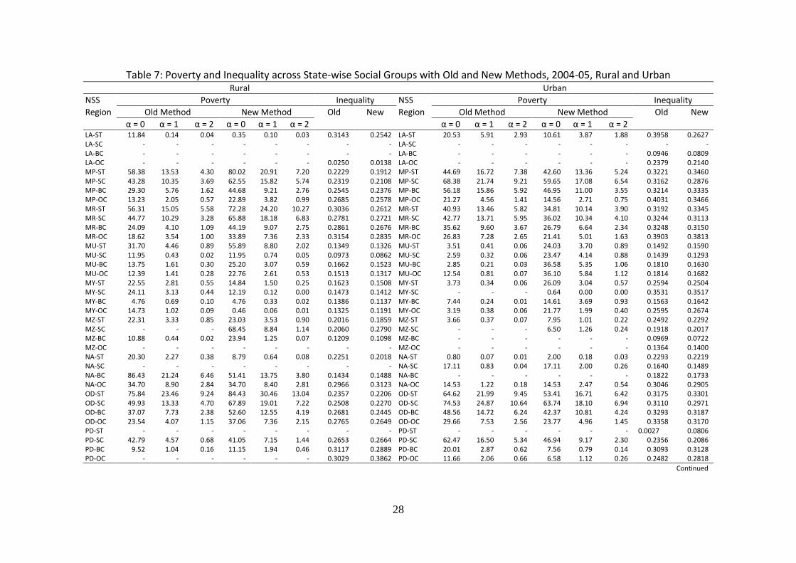
Poverty across social groups at all India level indicates an increase in incidence of poverty in

rural areas when we compare the computations in the old method to that of the new. For

scheduled tribes, scheduled castes, backward classes and other classes the percentage point

change (new minus old) is 16.6 per cent, 16.4 per cent, 14.0 per cent and 9.6 per cent

respectively; whereas the simple percentage change (percentage point change/old) is 36.6

per cent, 44.3 per cent, 54.0 per cent and 55.1 per cent respectively. The latter being higher

for lower bases even with lower percentage point increase is a statistical artefact and should

be left at that. In urban areas, the differences in incidence of poverty between the two

methods is less than one percentage point for each and every social group, but just to

mention, it has increased for scheduled tribes and other classes and decreased for

scheduled castes and backward classes.

26

Table 7: Poverty and Inequality across State-wise Social Groups with Old and New Methods, 2004-05, Rural and Urban

Rural Urban



α = 0 α = 1 α = 2 α = 0 α = 1 α = 2 α = 0 α = 1 α = 2 α = 0 α = 1 α = 2 AN-ST - - - - - - - - AN-ST - - - - - - - - AN-SC - - - - - - - - AN-SC - - - - - - - - AN-BC - - - - - - - - AN-BC - - - - - - - - AN-OC 22.65 3.25 0.80 3.32 0.22 0.02 0.3369 0.3089 AN-OC 22.45 3.76 0.90 0.83 0.01 0.00 0.3800 0.3435 AP-ST 28.29 6.90 2.91 60.29 17.50 7.08 0.2928 0.2629 AP-ST 51.90 13.30 4.59 50.11 11.73 3.88 0.3031 0.2732 AP-SC 15.52 2.86 1.04 41.83 9.29 3.14 0.2570 0.2325 AP-SC 37.37 7.78 2.18 34.99 6.80 1.82 0.3221 0.3074 AP-BC 8.64 1.44 0.42 31.60 6.18 1.81 0.2826 0.2490 AP-BC 28.69 5.73 1.83 23.80 4.85 1.60 0.3369 0.3249 AP-OC 3.76 0.46 0.10 16.15 2.95 0.79 0.2911 0.2733 AP-OC 20.21 4.45 1.44 16.49 3.52 1.07 0.4042 0.3917 AR-ST 19.23 4.17 1.35 29.68 6.77 2.39 0.2795 0.2593 AR-ST 4.69 0.96 0.29 23.47 5.81 1.98 0.2573 0.2518 AR-SC 2.97 0.30 0.03 2.97 0.66 0.15 0.1144 0.1076 AR-SC - - - 13.64 2.72 0.57 0.1166 0.1135 AR-BC 30.56 9.18 3.37 51.12 10.47 3.44 0.2087 0.1796 AR-BC - - - 8.77 1.53 0.27 0.0909 0.0915 AR-OC 31.22 4.54 1.15 46.36 9.52 2.62 0.2797 0.2683 AR-OC 3.53 0.24 0.03 26.99 4.54 0.99 0.2611 0.2444 AS-ST 12.62 1.74 0.37 28.76 4.11 0.99 0.1589 0.1556 AS-ST 2.93 0.14 0.01 29.80 6.51 1.54 0.2301 0.2455 AS-SC 25.71 4.42 1.11 45.32 8.85 2.49 0.1949 0.1893 AS-SC 5.09 1.42 0.48 37.24 7.20 2.04 0.2861 0.2853 AS-BC 18.15 3.27 0.81 31.92 6.59 1.88 0.2095 0.1994 AS-BC 5.39 0.53 0.09 26.74 5.57 1.64 0.4092 0.2986 AS-OC 26.10 4.32 1.14 38.75 7.86 2.33 0.2067 0.2006 AS-OC 2.87 0.26 0.04 15.58 2.85 0.74 0.2880 0.3044 BI-ST 56.19 6.65 1.01 59.33 12.96 3.13 0.1477 0.1575 BI-ST 57.24 5.60 0.55 57.24 12.18 2.59 0.2972 0.2931 BI-SC 64.17 13.69 3.87 77.64 20.11 6.65 0.1748 0.1657 BI-SC 66.85 17.47 5.88 71.20 24.38 9.67 0.4579 0.4513 BI-BC 38.52 7.22 1.97 52.64 11.46 3.48 0.1940 0.1822 BI-BC 40.25 7.63 2.16 49.64 12.20 3.84 0.2972 0.2752 BI-OC 26.36 3.70 0.82 35.75 6.62 1.65 0.2260 0.2024 BI-OC 17.22 3.57 1.14 22.98 5.45 1.89 0.2798 0.2682 CN-ST - - - - - - - - CN-ST 22.54 0.13 0.08 23.38 3.02 0.45 0.2628 0.3290 CN-SC - - - 1.98 0.42 0.09 0.2254 0.2306 CN-SC 15.62 1.98 0.32 28.22 4.90 1.14 0.3339 0.3344 CN-BC - - - 7.14 0.55 0.06 0.1852 0.1934 CN-BC 11.78 4.33 1.60 13.21 5.86 2.75 0.3283 0.3326 CN-OC 14.02 0.00 0.00 24.75 6.54 2.33 0.2309 0.2403 CN-OC 2.14 0.47 0.11 3.93 0.98 0.28 0.3280 0.3316 CT-ST 54.82 13.49 4.85 65.47 18.27 7.05 0.2731 0.2366 CT-ST 42.12 16.96 8.66 32.73 12.92 6.14 0.3914 0.3358 CT-SC 31.99 6.55 1.89 48.55 10.82 3.31 0.3297 0.2491 CT-SC 52.73 18.17 7.10 44.63 10.81 2.96 0.3310 0.3464 CT-BC 34.09 7.13 2.38 50.96 11.64 4.04 0.2855 0.2685 CT-BC 53.86 13.91 4.84 32.45 7.29 2.33 0.4357 0.3348 CT-OC 28.28 6.34 1.68 38.71 8.63 2.75 0.3119 0.3035 CT-OC 22.32 5.19 1.63 13.97 2.46 0.80 0.4356 0.3637 DA-ST 43.77 9.35 3.69 69.91 19.84 7.89 0.2895 0.2640 DA-ST 56.90 20.09 7.51 50.36 15.64 5.20 0.4206 0.3803 DA-SC - - - - - - 0.2377 0.2151 DA-SC 83.59 12.98 2.54 66.02 10.64 1.73 0.0646 0.0654 DA-BC 21.71 5.33 1.31 21.71 8.34 3.21 0.2776 0.3414 DA-BC - - - - - - 0.1063 0.0595 DA-OC 4.99 1.32 0.35 14.73 3.28 1.01 0.2638 0.2410 DA-OC 2.29 0.33 0.06 1.98 0.45 0.16 0.2301 0.2666 DD-ST 4.75 0.00 0.00 - - - 0.1322 0.1320 DD-ST 4.19 0.00 0.00 4.19 0.39 0.04 0.0482 0.0495 DD-SC - - - - - - 0.2498 0.2263 DD-SC 10.96 1.52 0.34 3.29 0.77 0.18 0.1841 0.1696 DD-BC 8.79 2.07 0.64 6.62 1.29 0.26 0.1636 0.1583 DD-BC 35.82 5.35 1.40 14.04 2.73 0.58 0.2296 0.2374 DD-OC - - - - - - 0.2550 0.2502 DD-OC 16.86 3.77 0.84 16.86 2.23 0.30 0.2584 0.2371

Continued

27


Rural Urban



α = 0 α = 1 α = 2 α = 0 α = 1 α = 2 α = 0 α = 1 α = 2 α = 0 α = 1 α = 2 DE-ST - - - - - - - - DE-ST - - - - - - 0.2221 0.2335 DE-SC - - - - - - 0.1338 0.1931 DE-SC 40.54 6.22 1.69 26.15 4.07 1.12 0.2314 0.2216 DE-BC - - - 27.01 0.75 0.02 0.1754 0.1727 DE-BC 20.26 3.21 0.80 22.70 3.28 0.83 0.2285 0.2377 DE-OC 10.63 0.47 0.02 15.51 2.74 0.53 0.2893 0.3118 DE-OC 6.28 1.13 0.31 6.14 0.99 0.25 0.3164 0.3164 GO-ST 49.83 0.46 0.00 49.83 18.17 6.63 0.4079 0.3225 GO-ST - - - - - - - - GO-SC - - - - - - 0.0780 0.1148 GO-SC 42.01 14.25 6.61 62.35 14.74 6.11 0.2855 0.2377 GO-BC 22.14 3.74 0.63 58.58 12.87 5.33 0.1833 0.2246 GO-BC 30.96 2.45 0.53 9.60 1.64 0.38 0.2177 0.2841 GO-OC 2.46 0.01 0.00 25.19 4.53 1.16 0.2994 0.2933 GO-OC 13.53 2.95 0.98 15.63 2.50 0.75 0.4282 0.3480 GU-ST 34.28 7.63 2.63 57.07 17.04 6.76 0.2640 0.2549 GU-ST 21.04 6.21 2.63 31.17 8.40 3.30 0.3042 0.4307 GU-SC 22.82 3.17 0.61 49.26 10.58 3.11 0.2191 0.2062 GU-SC 17.83 3.70 1.12 18.73 4.88 1.59 0.2647 0.2505 GU-BC 18.46 2.94 0.66 41.73 9.30 2.91 0.2350 0.2258 GU-BC 23.80 3.84 0.97 36.50 6.65 1.85 0.2784 0.2603 GU-OC 4.50 0.51 0.09 13.68 2.17 0.53 0.2721 0.2642 GU-OC 6.89 1.17 0.29 11.37 2.12 0.58 0.2966 0.2990 HA-ST 0.00 0.00 0.00 0.00 0.00 0.00 0.1160 0.1423 HA-ST 0.00 0.00 0.00 22.23 0.45 0.01 0.2963 0.2886 HA-SC 26.00 5.05 1.51 47.51 10.04 3.08 0.2316 0.2181 HA-SC 33.25 8.43 2.84 46.86 11.83 4.32 0.2778 0.2600 HA-BC 13.74 2.16 0.50 25.74 4.54 1.14 0.2727 0.2410 HA-BC 20.53 4.74 1.62 36.47 7.55 2.35 0.3447 0.2872 HA-OC 3.89 0.57 0.13 8.17 1.15 0.26 0.3628 0.3573 HA-OC 5.69 0.92 0.22 8.08 1.52 0.41 0.3405 0.3189 HP-ST 15.71 3.75 1.37 35.37 7.89 2.86 0.3460 0.3211 HP-ST 2.42 0.45 0.08 2.42 0.69 0.20 0.1700 0.1875 HP-SC 19.89 3.10 0.71 39.45 7.37 2.05 0.2653 0.2434 HP-SC 5.02 1.27 0.43 9.24 1.67 0.49 0.2343 0.2021 HP-BC 8.79 1.12 0.20 19.00 3.09 0.75 0.2471 0.2295 HP-BC 9.80 1.71 0.43 10.84 2.62 0.76 0.2023 0.1941 HP-OC 5.72 0.75 0.16 18.28 2.58 0.57 0.3232 0.3018 HP-OC 1.84 0.65 0.31 2.53 0.71 0.34 0.3321 0.2896 JK-ST - - - 26.52 3.03 0.35 0.2770 0.2695 JK-ST - - - - - - 0.2465 0.2873 JK-SC 4.54 0.57 0.09 14.71 1.67 0.35 0.2266 0.2095 JK-SC 10.79 2.15 0.58 13.79 2.13 0.49 0.2186 0.1975 JK-BC 9.78 1.91 0.45 23.52 4.55 1.37 0.2500 0.2073 JK-BC 3.12 0.88 0.25 3.12 0.81 0.21 0.1735 0.1456 JK-OC 3.05 0.38 0.11 11.78 1.65 0.37 0.2488 0.2178 JK-OC 7.38 1.73 0.50 10.50 2.20 0.59 0.2449 0.2515 JN-ST 54.12 12.63 3.98 60.56 14.64 4.83 0.2131 0.2116 JN-ST 42.49 11.32 3.69 47.20 14.12 5.07 0.3396 0.3278 JN-SC 57.55 13.70 4.36 60.97 14.95 4.79 0.2156 0.2071 JN-SC 48.78 8.33 2.17 52.55 10.64 3.08 0.3445 0.3020 JN-BC 40.00 7.63 2.05 46.67 8.49 2.28 0.2150 0.1886 JN-BC 17.39 3.69 1.15 21.98 5.42 1.81 0.2809 0.2822 JN-OC 36.92 7.31 2.13 37.45 8.02 2.33 0.2830 0.2452 JN-OC 8.22 1.79 0.58 10.30 2.38 0.78 0.3358 0.3049 KA-ST 21.39 2.23 0.40 50.53 8.11 1.77 0.1726 0.1581 KA-ST 61.87 20.02 9.50 55.70 16.28 6.90 0.3111 0.3084 KA-SC 31.33 4.64 1.04 57.37 10.63 2.92 0.2072 0.2114 KA-SC 50.32 15.83 6.62 41.22 11.39 4.40 0.2791 0.2715 KA-BC 20.80 3.16 0.75 35.85 6.27 1.63 0.2459 0.2340 KA-BC 38.23 10.21 3.60 32.14 7.21 2.30 0.3047 0.3108 KA-OC 13.69 1.57 0.31 23.72 3.81 0.91 0.3118 0.2677 KA-OC 20.96 4.77 1.62 14.31 3.24 1.06 0.3773 0.3748 KE-ST 40.15 17.31 9.63 56.86 23.21 12.24 0.3357 0.3277 KE-ST 21.79 3.10 0.69 21.79 3.66 1.35 0.3941 0.3771 KE-SC 21.63 3.95 1.10 30.82 6.80 2.11 0.3184 0.2741 KE-SC 33.40 6.50 2.19 33.00 8.11 3.08 0.2593 0.2735 KE-BC 13.55 2.62 0.80 21.34 4.31 1.30 0.3834 0.3397 KE-BC 23.99 5.73 1.99 21.19 4.77 1.54 0.4177 0.3690 KE-OC 7.14 1.54 0.67 10.82 2.18 0.84 0.3660 0.3462 KE-OC 7.17 1.38 0.43 7.86 1.25 0.34 0.3652 0.3929

Continued

28


Rural Urban



α = 0 α = 1 α = 2 α = 0 α = 1 α = 2 α = 0 α = 1 α = 2 α = 0 α = 1 α = 2 LA-ST 11.84 0.14 0.04 0.35 0.10 0.03 0.3143 0.2542 LA-ST 20.53 5.91 2.93 10.61 3.87 1.88 0.3958 0.2627 LA-SC - - - - - - - - LA-SC - - - - - - - - LA-BC - - - - - - - - LA-BC - - - - - - 0.0946 0.0809 LA-OC - - - - - - 0.0250 0.0138 LA-OC - - - - - - 0.2379 0.2140 MP-ST 58.38 13.53 4.30 80.02 20.91 7.20 0.2229 0.1912 MP-ST 44.69 16.72 7.38 42.60 13.36 5.24 0.3221 0.3460 MP-SC 43.28 10.35 3.69 62.55 15.82 5.74 0.2319 0.2108 MP-SC 68.38 21.74 9.21 59.65 17.08 6.54 0.3162 0.2876 MP-BC 29.30 5.76 1.62 44.68 9.21 2.76 0.2545 0.2376 MP-BC 56.18 15.86 5.92 46.95 11.00 3.55 0.3214 0.3335 MP-OC 13.23 2.05 0.57 22.89 3.82 0.99 0.2685 0.2578 MP-OC 21.27 4.56 1.41 14.56 2.71 0.75 0.4031 0.3466 MR-ST 56.31 15.05 5.58 72.28 24.20 10.27 0.3036 0.2612 MR-ST 40.93 13.46 5.82 34.81 10.14 3.90 0.3192 0.3345 MR-SC 44.77 10.29 3.28 65.88 18.18 6.83 0.2781 0.2721 MR-SC 42.77 13.71 5.95 36.02 10.34 4.10 0.3244 0.3113 MR-BC 24.09 4.10 1.09 44.19 9.07 2.75 0.2861 0.2676 MR-BC 35.62 9.60 3.67 26.79 6.64 2.34 0.3248 0.3150 MR-OC 18.62 3.54 1.00 33.89 7.36 2.33 0.3154 0.2835 MR-OC 26.83 7.28 2.65 21.41 5.01 1.63 0.3903 0.3813 MU-ST 31.70 4.46 0.89 55.89 8.80 2.02 0.1349 0.1326 MU-ST 3.51 0.41 0.06 24.03 3.70 0.89 0.1492 0.1590 MU-SC 11.95 0.43 0.02 11.95 0.74 0.05 0.0973 0.0862 MU-SC 2.59 0.32 0.06 23.47 4.14 0.88 0.1439 0.1293 MU-BC 13.75 1.61 0.30 25.20 3.07 0.59 0.1662 0.1523 MU-BC 2.85 0.21 0.03 36.58 5.35 1.06 0.1810 0.1630 MU-OC 12.39 1.41 0.28 22.76 2.61 0.53 0.1513 0.1317 MU-OC 12.54 0.81 0.07 36.10 5.84 1.12 0.1814 0.1682 MY-ST 22.55 2.81 0.55 14.84 1.50 0.25 0.1623 0.1508 MY-ST 3.73 0.34 0.06 26.09 3.04 0.57 0.2594 0.2504 MY-SC 24.11 3.13 0.44 12.19 0.12 0.00 0.1473 0.1412 MY-SC - - - 0.64 0.00 0.00 0.3531 0.3517 MY-BC 4.76 0.69 0.10 4.76 0.33 0.02 0.1386 0.1137 MY-BC 7.44 0.24 0.01 14.61 3.69 0.93 0.1563 0.1642 MY-OC 14.73 1.02 0.09 0.46 0.06 0.01 0.1325 0.1191 MY-OC 3.19 0.38 0.06 21.77 1.99 0.40 0.2595 0.2674 MZ-ST 22.31 3.33 0.85 23.03 3.53 0.90 0.2016 0.1859 MZ-ST 3.66 0.37 0.07 7.95 1.01 0.22 0.2492 0.2292 MZ-SC - - - 68.45 8.84 1.14 0.2060 0.2790 MZ-SC - - - 6.50 1.26 0.24 0.1918 0.2017 MZ-BC 10.88 0.44 0.02 23.94 1.25 0.07 0.1209 0.1098 MZ-BC - - - - - - 0.0969 0.0722 MZ-OC - - - - - - - - MZ-OC - - - - - - 0.1364 0.1400 NA-ST 20.30 2.27 0.38 8.79 0.64 0.08 0.2251 0.2018 NA-ST 0.80 0.07 0.01 2.00 0.18 0.03 0.2293 0.2219 NA-SC - - - - - - - - NA-SC 17.11 0.83 0.04 17.11 2.00 0.26 0.1640 0.1489 NA-BC 86.43 21.24 6.46 51.41 13.75 3.80 0.1434 0.1488 NA-BC - - - - - - 0.1822 0.1733 NA-OC 34.70 8.90 2.84 34.70 8.40 2.81 0.2966 0.3123 NA-OC 14.53 1.22 0.18 14.53 2.47 0.54 0.3046 0.2905 OD-ST 75.84 23.46 9.24 84.43 30.46 13.04 0.2357 0.2206 OD-ST 64.62 21.99 9.45 53.41 16.71 6.42 0.3175 0.3301 OD-SC 49.93 13.33 4.70 67.89 19.01 7.22 0.2508 0.2270 OD-SC 74.53 24.87 10.64 63.74 18.10 6.94 0.3110 0.2971 OD-BC 37.07 7.73 2.38 52.60 12.55 4.19 0.2681 0.2445 OD-BC 48.56 14.72 6.24 42.37 10.81 4.24 0.3293 0.3187 OD-OC 23.54 4.07 1.15 37.06 7.36 2.15 0.2765 0.2649 OD-OC 29.66 7.53 2.56 23.77 4.96 1.45 0.3358 0.3170 PD-ST - - - - - - - - PD-ST - - - - - - 0.0027 0.0806 PD-SC 42.79 4.57 0.68 41.05 7.15 1.44 0.2653 0.2664 PD-SC 62.47 16.50 5.34 46.94 9.17 2.30 0.2356 0.2086 PD-BC 9.52 1.04 0.16 11.15 1.94 0.46 0.3117 0.2889 PD-BC 20.01 2.87 0.62 7.56 0.79 0.14 0.3093 0.3128 PD-OC - - - - - - 0.3029 0.3862 PD-OC 11.66 2.06 0.66 6.58 1.12 0.26 0.2482 0.2818

Continued

29


Rural Urban



α = 0 α = 1 α = 2 α = 0 α = 1 α = 2 α = 0 α = 1 α = 2 α = 0 α = 1 α = 2 PN-ST 30.71 3.05 0.30 30.71 9.35 2.84 0.2030 0.2101 PN-ST 2.43 0.28 0.03 2.43 0.56 0.13 0.1316 0.1162 PN-SC 14.46 1.87 0.42 38.44 6.22 1.61 0.2433 0.2235 PN-SC 14.30 1.52 0.26 36.15 6.67 1.71 0.2635 0.2690 PN-BC 10.50 1.47 0.29 21.68 4.19 1.08 0.2952 0.2852 PN-BC 5.75 0.54 0.10 20.24 3.07 0.66 0.2835 0.2544 PN-OC 2.26 0.30 0.07 5.14 0.87 0.22 0.2689 0.2628 PN-OC 2.50 0.29 0.05 9.61 1.48 0.34 0.4207 0.3331 RA-ST 32.54 4.97 1.14 59.32 12.49 3.68 0.1861 0.1906 RA-ST 24.95 7.32 3.71 26.77 6.46 3.14 0.2682 0.2695 RA-SC 28.26 5.17 1.39 48.50 10.64 3.25 0.2537 0.2029 RA-SC 55.07 13.72 4.49 50.97 10.63 3.18 0.3447 0.2976 RA-BC 12.59 2.04 0.52 27.22 4.93 1.36 0.2511 0.2148 RA-BC 32.07 7.48 2.41 31.30 5.94 1.73 0.2904 0.2814 RA-OC 7.98 0.79 0.12 21.14 2.90 0.58 0.2281 0.2181 RA-OC 20.88 3.38 0.94 16.96 2.91 0.74 0.3972 0.3238 SI-ST 62.47 16.50 5.34 34.93 6.52 1.69 0.2611 0.2624 SI-ST 0.44 0.11 0.04 15.28 0.75 0.09 0.2478 0.2358 SI-SC 20.01 2.87 0.62 41.17 5.61 1.21 0.3148 0.2954 SI-SC 8.19 1.20 0.47 52.09 8.40 2.15 0.1739 0.1678 SI-BC 11.66 2.06 0.66 30.32 5.38 1.39 0.2818 0.2468 SI-BC 1.69 0.43 0.17 10.87 1.62 0.46 0.2529 0.2241 SI-OC 62.47 16.50 5.34 7.89 0.90 0.14 0.1547 0.1507 SI-OC 6.02 1.35 0.44 38.57 5.43 1.55 0.2427 0.2318 TN-ST 27.18 0.94 0.05 47.26 10.17 2.45 0.1904 0.2193 TN-ST 33.09 11.28 4.69 34.71 10.98 4.48 0.3303 0.3417 TN-SC 30.37 5.21 1.47 51.24 10.18 3.02 0.2387 0.2148 TN-SC 41.22 9.30 2.99 40.74 8.97 2.83 0.3096 0.2827 TN-BC 20.24 3.28 0.82 32.61 6.40 1.79 0.3324 0.2801 TN-BC 20.82 4.20 1.28 17.32 3.42 1.00 0.3307 0.3350 TN-OC 18.81 3.59 0.88 22.22 5.55 1.70 0.4724 0.3944 TN-OC 6.96 1.39 0.35 6.51 1.64 0.61 0.3641 0.3636 TR-ST 27.60 4.05 1.01 53.44 11.30 3.51 0.1827 0.1792 TR-ST - - - 3.90 0.58 0.09 0.2249 0.2210 TR-SC 22.59 3.47 0.82 45.00 10.04 3.03 0.2088 0.1919 TR-SC 9.26 1.23 0.19 38.49 7.21 2.11 0.2659 0.2451 TR-BC 17.93 2.62 0.67 37.88 7.76 2.21 0.2239 0.2106 TR-BC 1.82 0.18 0.03 34.19 5.34 1.05 0.2980 0.2814 TR-OC 19.67 3.22 0.81 41.06 8.92 2.72 0.2372 0.2400 TR-OC 2.29 0.27 0.08 14.19 2.37 0.61 0.3620 0.3260 UP-ST 32.18 3.20 0.54 41.99 5.93 1.25 0.1936 0.2039 UP-ST 37.59 9.83 3.80 40.30 10.55 3.84 0.4415 0.3969 UP-SC 44.73 9.06 2.72 56.60 12.79 4.02 0.2610 0.2221 UP-SC 43.46 10.81 3.64 44.24 11.59 3.92 0.2972 0.2829 UP-BC 32.90 6.04 1.66 42.18 8.85 2.61 0.2796 0.2436 UP-BC 36.03 8.69 2.97 42.73 9.78 3.19 0.3068 0.2840 UP-OC 19.48 3.57 1.02 26.02 5.32 1.58 0.3166 0.2739 UP-OC 18.96 3.93 1.18 20.86 4.29 1.31 0.3973 0.3834 UT-ST 44.55 7.05 1.69 32.44 4.82 0.98 0.2006 0.1954 UT-ST 69.03 6.15 0.93 39.05 4.06 0.60 0.2526 0.2574 UT-SC 53.28 10.90 3.14 46.24 8.55 2.25 0.2490 0.2258 UT-SC 70.12 16.97 5.53 47.46 10.15 2.95 0.3015 0.2882 UT-BC 44.41 9.61 2.62 43.46 7.35 1.83 0.2668 0.2303 UT-BC 43.94 10.47 3.32 34.97 7.06 1.93 0.2353 0.2330 UT-OC 33.54 5.89 1.55 27.89 4.21 0.97 0.3032 0.2434 UT-OC 25.06 5.75 1.66 17.93 3.23 0.87 0.3260 0.3102 WB-ST 42.74 8.58 2.45 54.31 12.31 3.79 0.2051 0.1897 WB-ST 22.19 2.60 0.47 47.96 9.02 2.13 0.3322 0.3335 WB-SC 28.85 5.03 1.28 37.14 7.53 2.19 0.2405 0.2323 WB-SC 25.46 4.35 1.12 40.95 8.92 2.76 0.3161 0.2874 WB-BC 17.68 3.95 1.40 28.32 5.66 1.89 0.2839 0.2643 WB-BC 7.36 1.61 0.52 23.64 4.99 1.52 0.3268 0.3296 WB-OC 27.35 5.14 1.42 37.70 7.77 2.29 0.2903 0.2673 WB-OC 10.47 2.02 0.57 19.53 4.25 1.34 0.3843 0.3756 AI-ST 45.54 10.77 3.71 62.17 16.97 6.33 0.2717 0.2537 AI-ST 34.63 10.91 4.69 35.52 9.93 3.81 0.3390 0.3513 AI-SC 37.08 7.49 2.23 53.52 12.25 3.96 0.2634 0.2405 AI-SC 40.88 10.39 3.79 40.56 9.85 3.38 0.3168 0.3016 AI-BC 25.83 4.73 1.30 39.79 8.23 2.46 0.2938 0.2649 AI-BC 31.05 7.32 2.50 30.62 6.72 2.14 0.3362 0.3263 AI-OC 17.46 3.00 0.81 27.08 5.27 1.51 0.3200 0.2990 AI-OC 16.11 3.63 1.18 16.13 3.39 1.04 0.3804 0.3659 AI 28.12 5.50 1.63 41.80 9.24 2.94 0.3045 0.2808 AI 25.84 6.21 2.16 25.68 5.78 1.88 0.3764 0.3643 Note: The first two letters represent the state code as in Table 5 and the last two represent social groups: ST=Scheduled Tribes, SC=Scheduled Classes, BC=Backward Classes and OC=Other Classes. All estimates are based on unit level data, see notes in Tables 1 and 4. Source: Unit level data, Schedule 1.0, NSS 61st Round, 2004-05.

30

Table 8: Poverty and Inequality across State-wise Occupation Groups with Old and New Methods, 2004-05, Rural and Urban Rural Urban



α = 0 α = 1 α = 2 α = 0 α = 1 α = 2 α = 0 α = 1 α = 2 α = 0 α = 1 α = 2 AN-O1 12.74 2.16 0.63 5.38 0.33 0.02 0.5381 0.4614 AN-O1 24.35 3.94 0.80 - - - 0.2697 0.2935 AN-O2 47.59 7.51 2.06 6.52 0.80 0.10 0.2276 0.1779 AN-O2 14.68 1.96 0.40 - - - 0.4006 0.3488 AN-O3 22.35 2.52 0.58 2.62 0.13 0.01 0.1851 0.1754 AN-O3 55.23 11.31 3.15 5.58 0.08 0.00 0.1956 0.1990 AN-O4 34.47 5.40 1.29 4.74 0.25 0.01 0.2142 0.1908 AN-O4 - - - - - - - - AN-O9 3.59 0.25 0.03 - - - 0.2408 0.2459 AN-O9 5.29 1.53 0.55 - - - 0.2343 0.2496 AP-O1 4.71 0.83 0.21 22.40 4.09 1.16 0.2903 0.2630 AP-O1 31.95 6.26 1.81 26.53 5.24 1.47 0.3356 0.3313 AP-O2 15.93 2.49 0.58 46.07 9.95 3.08 0.2314 0.2062 AP-O2 17.05 3.27 0.92 13.98 2.56 0.69 0.3556 0.3372 AP-O3 6.32 0.98 0.25 27.78 5.18 1.43 0.2622 0.2238 AP-O3 49.84 11.44 3.61 45.24 9.67 2.96 0.2604 0.1925 AP-O4 8.78 1.37 0.35 26.05 5.51 1.69 0.3007 0.2720 AP-O4 - - - - - - - - AP-O9 8.74 4.78 3.51 18.45 6.70 3.80 0.3600 0.3285 AP-O9 13.09 5.06 3.17 13.05 5.31 3.36 0.4769 0.4552 AR-O1 15.55 2.35 0.55 18.37 3.71 0.97 0.3049 0.2718 AR-O1 2.00 0.14 0.01 19.83 3.59 0.78 0.2338 0.2138 AR-O2 17.60 6.46 2.77 33.68 6.70 2.54 0.2195 0.2260 AR-O2 2.35 0.13 0.01 16.98 3.14 0.81 0.2435 0.2305 AR-O3 51.42 10.42 3.63 55.33 17.62 7.11 0.2318 0.2414 AR-O3 11.01 2.15 0.56 80.31 15.04 4.01 0.1919 0.1321 AR-O4 22.43 4.18 1.23 37.00 7.62 2.40 0.2624 0.2474 AR-O4 - - - - - - - - AR-O9 19.14 4.88 1.71 24.60 7.21 2.80 0.2769 0.2597 AR-O9 12.88 3.12 1.02 45.58 12.72 4.73 0.2862 0.2929 AS-O1 26.99 4.64 1.16 40.39 8.22 2.38 0.2115 0.2019 AS-O1 3.66 0.48 0.11 24.77 4.66 1.19 0.3039 0.3224 AS-O2 36.64 6.47 1.76 55.37 11.88 3.57 0.1670 0.1616 AS-O2 1.00 0.06 0.01 15.58 2.47 0.58 0.3237 0.2791 AS-O3 39.26 7.71 2.27 61.27 13.70 4.29 0.1800 0.1680 AS-O3 23.21 3.28 0.88 77.87 19.27 6.12 0.1536 0.1554 AS-O4 15.60 2.13 0.45 28.67 4.76 1.21 0.1684 0.1640 AS-O4 - - - - - - - - AS-O9 9.68 1.66 0.53 15.21 2.85 0.89 0.2479 0.2308 AS-O9 3.99 0.48 0.09 10.85 2.62 0.82 0.2550 0.2705 BI-O1 37.00 5.74 1.40 52.63 10.00 2.78 0.1837 0.1748 BI-O1 36.03 6.87 1.93 47.17 11.31 3.54 0.2726 0.2732 BI-O2 67.48 14.51 4.19 79.29 21.16 7.11 0.1576 0.1562 BI-O2 25.19 4.31 1.01 28.39 7.10 2.19 0.3562 0.3150 BI-O3 58.69 9.24 2.24 78.28 16.07 4.65 0.1459 0.1424 BI-O3 80.74 22.37 8.23 83.22 28.94 11.90 0.2488 0.2395 BI-O4 25.52 4.29 1.07 37.75 7.17 1.93 0.2006 0.1803 BI-O4 - - - - - - - - BI-O9 41.62 8.61 2.40 54.95 13.14 4.14 0.2514 0.2320 BI-O9 23.40 4.84 1.56 26.48 7.02 2.56 0.3618 0.3518 CN-O1 16.78 0.01 0.00 29.61 7.83 2.79 0.2750 0.2872 CN-O1 10.07 1.67 0.51 15.90 3.73 1.19 0.3742 0.3954 CN-O2 - - - - - - - - CN-O2 4.58 0.83 0.18 7.88 1.60 0.43 0.3342 0.3280 CN-O3 - - - - - - 0.0059 0.0088 CN-O3 16.48 3.92 0.93 17.99 6.17 2.26 0.1163 0.1092 CN-O4 - - - 13.15 1.01 0.11 0.2442 0.2665 CN-O4 - - - - - - - - CN-O9 - - - 1.25 0.27 0.06 0.1868 0.1853 CN-O9 - - - - - - 0.2908 0.3165 CT-O1 43.96 13.49 5.80 51.33 17.12 8.00 0.3433 0.3447 CT-O1 43.23 11.89 4.63 25.11 6.47 2.41 0.3699 0.3198 CT-O2 55.45 12.49 4.05 73.28 18.92 6.62 0.2351 0.2087 CT-O2 24.12 7.07 2.61 17.36 4.00 1.34 0.4663 0.3671 CT-O3 24.04 4.48 1.56 38.11 8.26 2.82 0.2210 0.2126 CT-O3 92.02 29.05 11.78 71.08 18.94 6.85 0.1676 0.1808 CT-O4 32.01 6.85 2.29 44.59 10.04 3.48 0.2896 0.2532 CT-O4 - - - - - - - - CT-O9 16.65 3.70 1.22 28.22 5.32 1.83 0.4112 0.3101 CT-O9 18.70 4.30 1.31 8.37 1.67 0.46 0.3687 0.3736

Continued

31




α = 0 α = 1 α = 2 α = 0 α = 1 α = 2 α = 0 α = 1 α = 2 α = 0 α = 1 α = 2 DA-O1 14.82 1.67 0.19 29.37 7.31 2.00 0.3238 0.3221 DA-O1 1.99 0.40 0.08 1.06 0.19 0.03 0.1840 0.1861 DA-O2 84.34 11.01 2.00 93.30 30.00 10.22 0.1325 0.1347 DA-O2 22.83 8.13 3.23 22.71 7.26 2.58 0.3270 0.3521 DA-O3 40.30 7.52 1.68 66.26 18.26 6.18 0.2960 0.2767 DA-O3 96.25 27.62 8.26 68.75 17.11 4.30 0.0450 0.0640 DA-O4 34.55 2.89 0.37 71.60 13.94 3.68 0.2709 0.2015 DA-O4 - - - - - - - - DA-O9 30.30 18.66 12.55 48.37 20.27 13.81 0.4184 0.3944 DA-O9 - - - - - - - - DD-O1 7.48 0.03 0.00 - - - 0.0967 0.1005 DD-O1 6.71 1.85 0.58 5.62 1.19 0.26 0.1450 0.1366 DD-O2 1.56 0.01 0.00 - - - 0.0438 0.0477 DD-O2 8.69 0.68 0.13 1.30 0.26 0.05 0.2811 0.2616 DD-O3 18.81 5.89 1.84 18.81 3.81 0.77 0.1536 0.1330 DD-O3 76.99 16.25 3.58 72.74 9.50 1.25 0.1002 0.0945 DD-O4 6.05 0.15 0.04 0.53 0.03 0.00 0.1123 0.0922 DD-O4 - - - - - - - - DD-O9 - - - - - - 0.2746 0.2679 DD-O9 43.34 3.53 0.29 14.45 0.01 0.00 0.2389 0.2273 DE-O1 22.89 1.01 0.05 41.20 5.41 1.06 0.2048 0.2127 DE-O1 17.34 2.51 0.55 12.11 1.59 0.32 0.3226 0.3092 DE-O2 - - - - - - 0.0163 0.0182 DE-O2 12.20 1.81 0.44 9.53 1.44 0.32 0.3307 0.3373 DE-O3 - - - 46.15 4.35 0.41 0.1017 0.0977 DE-O3 57.89 12.31 4.77 57.85 10.43 4.03 0.2305 0.2184 DE-O4 - - - - - - 0.1071 0.0816 DE-O4 - - - - - - - - DE-O9 - - - - - - 0.2685 0.2860 DE-O9 6.41 2.64 1.09 9.01 3.82 1.63 0.3780 0.3653 GO-O1 - - - 4.20 0.81 0.18 0.3399 0.2319 GO-O1 13.64 2.34 0.68 9.79 1.84 0.52 0.4624 0.3438 GO-O2 19.24 3.25 0.55 57.24 13.79 5.35 0.2647 0.2390 GO-O2 9.87 2.32 0.88 13.22 2.05 0.66 0.3612 0.3341 GO-O3 10.60 0.08 0.00 26.00 5.83 1.79 0.2436 0.2452 GO-O3 64.62 17.68 7.59 82.29 17.68 6.87 0.2008 0.1688 GO-O4 4.25 0.01 0.00 41.98 9.16 2.51 0.2632 0.2344 GO-O4 - - - - - - - - GO-O9 - - - 25.59 3.17 0.66 0.2999 0.3103 GO-O9 10.50 1.38 0.18 6.63 0.33 0.02 0.2226 0.2397 GU-O1 10.35 1.58 0.35 28.01 5.45 1.63 0.3023 0.2556 GU-O1 13.93 2.42 0.63 21.45 4.00 1.14 0.2932 0.2923 GU-O2 29.59 5.00 1.24 57.77 14.50 4.81 0.2007 0.1895 GU-O2 7.18 1.22 0.32 11.87 2.17 0.60 0.3027 0.3041 GU-O3 22.12 4.23 1.12 45.87 11.41 3.87 0.2448 0.2440 GU-O3 47.40 8.46 2.38 62.89 13.80 4.16 0.2146 0.2042 GU-O4 13.32 2.36 0.69 27.35 6.33 2.22 0.2642 0.2641 GU-O4 - - - - - - - - GU-O9 5.60 2.07 1.19 18.36 3.47 1.50 0.3008 0.2867 GU-O9 5.16 2.37 1.39 6.96 2.70 1.43 0.3646 0.3905 HA-O1 11.68 2.38 0.66 24.89 4.99 1.44 0.2668 0.2303 HA-O1 11.59 2.44 0.76 18.29 3.82 1.22 0.3432 0.3263 HA-O2 27.97 5.62 1.64 59.36 11.34 3.37 0.2007 0.1677 HA-O2 11.90 2.26 0.60 19.60 3.71 1.01 0.3685 0.3299 HA-O3 31.71 5.60 1.66 48.48 10.42 3.11 0.2556 0.2107 HA-O3 50.27 14.59 5.60 67.06 19.84 7.76 0.2443 0.2196 HA-O4 5.32 0.80 0.16 11.57 1.66 0.37 0.2536 0.2168 HA-O4 - - - - - - - - HA-O9 8.16 0.81 0.16 10.97 2.18 0.52 0.4613 0.4745 HA-O9 5.81 1.27 0.36 13.95 1.58 0.49 0.3839 0.3718 HP-O1 9.63 1.08 0.20 21.85 3.10 0.70 0.3983 0.3435 HP-O1 2.78 0.57 0.18 4.43 0.79 0.24 0.2690 0.2360 HP-O2 35.03 4.50 0.72 54.23 11.56 3.12 0.2505 0.2274 HP-O2 1.22 0.16 0.03 1.45 0.22 0.04 0.3267 0.2755 HP-O3 18.91 3.00 0.69 41.92 7.66 2.13 0.2101 0.2033 HP-O3 12.42 4.49 2.01 16.99 5.21 2.33 0.2586 0.2304 HP-O4 9.30 1.51 0.40 24.08 3.98 1.04 0.2668 0.2589 HP-O4 - - - - - - - - HP-O9 1.86 0.24 0.05 6.10 0.84 0.20 0.3171 0.2916 HP-O9 - - - - - - 0.2737 0.2533

Continued

32




α = 0 α = 1 α = 2 α = 0 α = 1 α = 2 α = 0 α = 1 α = 2 α = 0 α = 1 α = 2 JK-O1 3.31 0.43 0.11 14.76 2.07 0.51 0.2445 0.2222 JK-O1 5.14 0.84 0.22 5.40 0.78 0.19 0.2221 0.2114 JK-O2 10.89 1.16 0.18 17.22 3.61 0.90 0.1532 0.1484 JK-O2 2.19 0.35 0.08 3.41 0.59 0.14 0.2226 0.2366 JK-O3 11.20 1.10 0.20 31.29 4.55 1.03 0.1590 0.1526 JK-O3 41.92 12.02 3.64 42.65 12.50 3.90 0.1633 0.1547 JK-O4 2.25 0.43 0.13 11.94 1.55 0.36 0.2438 0.1991 JK-O4 - - - - - - - - JK-O9 5.52 1.04 0.23 9.43 2.00 0.59 0.2594 0.2427 JK-O9 1.49 0.12 0.01 22.22 2.81 0.36 0.2404 0.2913 JN-O1 41.59 7.54 2.01 45.77 8.54 2.32 0.2473 0.2122 JN-O1 19.37 4.27 1.30 24.87 5.80 1.85 0.3286 0.2790 JN-O2 75.13 20.50 7.14 78.00 21.40 7.59 0.1944 0.1852 JN-O2 8.92 2.14 0.68 11.71 2.93 0.99 0.3477 0.3371 JN-O3 60.16 12.54 3.52 67.99 14.40 4.10 0.1778 0.1600 JN-O3 61.58 11.98 3.65 65.81 15.95 5.33 0.2447 0.2684 JN-O4 43.97 9.31 2.76 50.63 10.77 3.30 0.2063 0.1902 JN-O4 - - - - - - - - JN-O9 16.28 2.83 0.66 17.14 2.75 0.56 0.2316 0.2122 JN-O9 8.25 1.81 0.46 8.43 2.34 0.73 0.2147 0.2064 KA-O1 13.15 1.74 0.36 24.73 3.77 0.84 0.2609 0.2330 KA-O1 32.23 8.05 2.82 25.25 5.30 1.64 0.3215 0.3244 KA-O2 32.40 4.83 1.13 56.27 10.63 2.87 0.1815 0.1629 KA-O2 20.25 4.67 1.54 14.13 2.95 0.90 0.3616 0.3538 KA-O3 10.67 2.20 0.59 23.98 4.50 1.47 0.2174 0.2057 KA-O3 64.69 20.52 8.53 56.75 16.30 6.06 0.2622 0.2484 KA-O4 14.08 1.51 0.25 26.97 3.91 0.82 0.2594 0.2388 KA-O4 - - - - - - - - KA-O9 9.10 1.03 0.38 17.11 2.73 0.79 0.4513 0.3964 KA-O9 27.69 7.50 2.80 22.04 5.60 2.63 0.4329 0.4481 KE-O1 7.65 1.16 0.27 11.61 1.99 0.52 0.3601 0.3413 KE-O1 15.14 3.56 1.26 13.67 3.01 1.01 0.4131 0.3940 KE-O2 23.91 5.13 1.79 35.79 8.52 3.04 0.2988 0.2414 KE-O2 14.55 3.32 1.11 12.96 2.64 0.78 0.3899 0.3822 KE-O3 17.16 4.03 1.48 26.54 6.06 2.10 0.3082 0.2830 KE-O3 31.74 7.64 2.62 32.01 7.44 2.50 0.3237 0.2845 KE-O4 5.75 0.55 0.10 10.21 1.29 0.24 0.3983 0.3633 KE-O4 - - - - - - - - KE-O9 9.41 2.22 0.95 13.17 3.10 1.16 0.4217 0.3648 KE-O9 18.03 2.47 0.78 10.48 1.70 0.53 0.3948 0.4030 LA-O1 - - - - - - 0.1834 0.1663 LA-O1 18.11 3.42 0.88 4.49 1.01 0.23 0.3063 0.2335 LA-O2 - - - - - - 0.0000 0.0000 LA-O2 10.97 0.77 0.11 0.87 0.04 0.00 0.3876 0.2087 LA-O3 - - - - - - 0.2586 0.1948 LA-O3 62.40 30.35 17.66 54.20 23.68 12.32 0.4478 0.4397 LA-O4 0.67 0.16 0.05 0.46 0.13 0.04 0.2657 0.2647 LA-O4 - - - - - - - - LA-O9 29.15 0.16 0.05 0.35 0.10 0.03 0.2619 0.2065 LA-O9 19.17 6.05 2.01 19.17 3.30 0.77 0.2979 0.3172 MP-O1 32.67 6.88 2.26 45.07 10.25 3.38 0.2691 0.2477 MP-O1 48.36 13.29 4.89 37.52 8.94 2.92 0.4088 0.3387 MP-O2 56.52 13.73 4.69 76.93 20.72 7.43 0.2215 0.1925 MP-O2 25.33 5.47 1.90 19.27 4.03 1.31 0.3367 0.3482 MP-O3 49.56 11.08 3.47 67.36 17.61 6.26 0.2378 0.2067 MP-O3 78.57 27.36 11.59 74.61 20.91 7.74 0.2625 0.2140 MP-O4 27.13 5.10 1.36 43.40 8.55 2.44 0.2558 0.2392 MP-O4 - - - - - - - - MP-O9 11.80 2.50 0.92 20.13 4.00 1.44 0.2793 0.2875 MP-O9 30.72 9.96 3.71 25.83 6.37 1.96 0.5082 0.4358 MR-O1 21.37 3.62 0.96 36.89 8.08 2.53 0.3210 0.2945 MR-O1 32.79 9.19 3.52 26.40 6.44 2.22 0.3774 0.3775 MR-O2 47.32 10.39 3.18 69.46 18.63 6.78 0.2285 0.2064 MR-O2 23.04 5.60 1.91 17.10 3.56 1.06 0.3488 0.3314 MR-O3 30.88 5.95 1.69 46.05 12.19 4.30 0.3065 0.2796 MR-O3 76.73 26.24 11.42 66.56 20.51 8.14 0.2472 0.2418 MR-O4 18.18 3.96 1.37 35.51 7.72 2.67 0.2884 0.2529 MR-O4 - - - - - - - - MR-O9 7.97 2.05 1.05 16.58 3.92 1.63 0.3307 0.3185 MR-O9 13.72 3.96 1.81 9.50 2.91 1.27 0.4072 0.3843

Continued

33




α = 0 α = 1 α = 2 α = 0 α = 1 α = 2 α = 0 α = 1 α = 2 α = 0 α = 1 α = 2 MU-O1 14.09 2.18 0.46 24.24 3.07 0.70 0.1743 0.1515 MU-O1 5.09 0.41 0.06 43.67 6.89 1.43 0.1625 0.1498 MU-O2 7.02 2.10 0.65 25.31 2.90 0.94 0.1303 0.1249 MU-O2 1.34 0.10 0.01 17.35 2.31 0.42 0.1805 0.1582 MU-O3 25.67 2.54 0.56 50.49 6.88 1.49 0.1356 0.1276 MU-O3 9.47 0.66 0.05 66.58 13.56 3.00 0.1281 0.1430 MU-O4 25.96 3.59 0.71 47.74 7.08 1.58 0.1259 0.1236 MU-O4 - - - - - - - - MU-O9 18.11 1.52 0.20 26.62 4.04 0.77 0.1910 0.1917 MU-O9 1.70 0.18 0.04 38.67 4.60 0.89 0.1706 0.1654 MY-O1 14.00 1.51 0.26 6.64 0.72 0.11 0.1697 0.1634 MY-O1 7.05 0.67 0.11 30.51 4.65 1.10 0.1997 0.2367 MY-O2 30.91 4.28 0.90 24.12 2.44 0.45 0.1332 0.1175 MY-O2 0.95 0.08 0.01 19.48 1.70 0.26 0.2539 0.2469 MY-O3 31.99 3.43 0.54 23.01 2.16 0.30 0.1191 0.1156 MY-O3 19.50 1.98 0.31 66.09 9.61 1.92 0.1796 0.1501 MY-O4 24.25 2.93 0.57 15.05 1.51 0.24 0.1489 0.1293 MY-O4 - - - - - - - - MY-O9 6.20 0.87 0.16 2.63 0.28 0.06 0.1747 0.1652 MY-O9 3.46 0.30 0.06 20.81 1.98 0.35 0.2973 0.2968 MZ-O1 5.87 0.85 0.18 6.63 0.96 0.21 0.2387 0.2062 MZ-O1 5.54 0.45 0.08 12.14 1.48 0.30 0.2400 0.2195 MZ-O2 5.80 0.29 0.01 - - - 0.1796 0.1485 MZ-O2 1.02 0.14 0.03 2.69 0.37 0.09 0.2321 0.2150 MZ-O3 13.85 3.78 1.58 7.20 3.19 1.41 0.1579 0.1622 MZ-O3 9.93 1.39 0.27 19.06 2.78 0.69 0.1939 0.1842 MZ-O4 26.46 3.91 1.00 27.33 4.20 1.08 0.1702 0.1536 MZ-O4 - - - - - - - - MZ-O9 8.52 1.32 0.30 11.05 1.18 0.21 0.1997 0.2028 MZ-O9 4.58 0.52 0.07 9.19 1.04 0.19 0.2498 0.2205 NA-O1 20.40 4.63 1.39 15.57 2.99 0.79 0.2693 0.2678 NA-O1 6.76 0.52 0.07 7.67 1.06 0.21 0.2550 0.2551 NA-O2 57.23 21.08 7.77 57.23 21.42 8.02 0.2027 0.1718 NA-O2 - - - 1.36 0.07 0.00 0.2287 0.2120 NA-O3 - - - - - - 0.0671 0.0633 NA-O3 8.93 0.70 0.05 8.93 1.08 0.13 0.1606 0.1518 NA-O4 31.04 3.59 0.62 13.09 1.05 0.15 0.1639 0.1277 NA-O4 - - - - - - - - NA-O9 2.97 0.18 0.01 0.81 0.03 0.00 0.2256 0.2023 NA-O9 7.73 0.43 0.03 5.83 1.00 0.17 0.2596 0.2582 OD-O1 32.78 7.71 2.52 47.07 11.90 4.20 0.2762 0.2593 OD-O1 50.16 15.71 6.44 44.42 11.53 4.29 0.3283 0.3190 OD-O2 64.54 18.27 6.87 78.98 24.86 10.04 0.2369 0.2082 OD-O2 20.90 4.28 1.28 14.07 2.58 0.72 0.3151 0.2838 OD-O3 51.95 14.36 5.50 71.50 21.25 8.62 0.2533 0.2324 OD-O3 89.25 29.33 12.42 76.15 21.19 7.81 0.2221 0.2095 OD-O4 46.11 11.10 3.78 58.95 16.06 5.81 0.2573 0.2379 OD-O4 - - - - - - - - OD-O9 19.78 3.66 1.08 28.53 6.35 2.08 0.3087 0.2976 OD-O9 26.38 7.66 3.49 22.10 5.79 2.55 0.3651 0.3926 PD-O1 - - - 2.52 0.04 0.00 0.2761 0.2088 PD-O1 17.20 1.89 0.35 6.19 0.68 0.10 0.2862 0.2853 PD-O2 41.67 4.16 0.58 43.25 8.09 1.72 0.3068 0.2488 PD-O2 14.88 2.28 0.47 4.73 0.45 0.08 0.2978 0.3079 PD-O3 20.49 2.48 0.36 14.94 2.32 0.41 0.2934 0.2316 PD-O3 48.23 9.96 2.90 27.46 4.40 1.04 0.3054 0.2378 PD-O4 - - - 4.97 0.12 0.00 0.2649 0.2692 PD-O4 - - - - - - - - PD-O9 13.74 2.35 0.82 13.74 3.15 1.09 0.4672 0.5187 PD-O9 13.41 2.84 0.82 9.10 1.02 0.28 0.3395 0.3856 PN-O1 6.44 1.03 0.24 17.58 2.81 0.69 0.2906 0.2569 PN-O1 4.74 0.56 0.11 15.80 2.66 0.66 0.3350 0.3211 PN-O2 25.78 3.13 0.64 54.97 9.76 2.53 0.1983 0.1720 PN-O2 4.63 0.45 0.07 17.16 2.64 0.55 0.4675 0.3282 PN-O3 9.54 1.67 0.40 31.05 5.25 1.45 0.2282 0.2184 PN-O3 25.48 2.60 0.47 50.42 9.88 2.75 0.1963 0.1912 PN-O4 0.94 0.03 0.00 1.90 0.23 0.04 0.2457 0.2431 PN-O4 - - - - - - - - PN-O9 1.86 0.09 0.01 6.80 0.90 0.16 0.3282 0.3152 PN-O9 8.90 0.73 0.09 17.05 3.28 0.72 0.4503 0.4339

Continued

34




α = 0 α = 1 α = 2 α = 0 α = 1 α = 2 α = 0 α = 1 α = 2 α = 0 α = 1 α = 2 RA-O1 12.61 1.86 0.40 27.79 5.05 1.29 0.2432 0.2158 RA-O1 37.75 7.24 2.04 31.88 5.20 1.34 0.3003 0.2811 RA-O2 37.03 6.17 1.44 61.85 13.61 4.04 0.2264 0.1742 RA-O2 18.27 3.91 1.14 17.83 3.37 0.86 0.4078 0.3141 RA-O3 34.72 5.57 1.39 60.34 12.87 3.77 0.2371 0.1978 RA-O3 63.41 19.20 7.40 62.52 16.69 5.78 0.2427 0.2401 RA-O4 14.09 2.32 0.60 29.75 5.51 1.57 0.2389 0.2083 RA-O4 - - - - - - - - RA-O9 7.49 1.20 0.34 18.72 2.93 0.86 0.2440 0.2378 RA-O9 12.58 3.06 1.57 19.72 3.31 1.47 0.3968 0.4155 SI-O1 10.36 1.72 0.48 16.85 2.74 0.80 0.2141 0.2127 SI-O1 2.63 0.64 0.17 40.64 4.86 1.07 0.2257 0.2177 SI-O2 71.17 11.83 2.44 72.85 17.43 4.70 0.1624 0.1582 SI-O2 2.80 0.59 0.25 18.68 2.10 0.58 0.2628 0.2430 SI-O3 22.87 3.82 0.85 31.68 6.39 1.78 0.2445 0.2411 SI-O3 11.55 1.21 0.23 20.98 5.74 1.86 0.1236 0.1253 SI-O4 32.27 4.92 1.05 45.15 7.89 1.95 0.1858 0.1599 SI-O4 - - - - - - - - SI-O9 2.98 0.53 0.13 9.21 1.06 0.22 0.2877 0.2625 SI-O9 4.68 1.85 0.83 5.38 2.57 1.53 0.2713 0.2492 TN-O1 12.72 1.84 0.44 24.65 4.00 1.02 0.3703 0.2982 TN-O1 21.09 4.24 1.25 18.61 3.96 1.18 0.3436 0.3435 TN-O2 33.64 5.74 1.46 54.30 11.23 3.25 0.2140 0.1873 TN-O2 15.36 2.95 0.84 12.21 2.21 0.59 0.3448 0.3393 TN-O3 20.86 3.36 0.79 34.25 6.78 1.91 0.2672 0.2297 TN-O3 53.01 11.99 3.95 49.88 10.90 3.53 0.2037 0.2159 TN-O4 15.65 1.84 0.33 23.84 4.06 0.94 0.3144 0.2605 TN-O4 - - - - - - - - TN-O9 10.60 3.01 1.56 17.12 3.98 1.69 0.4115 0.3346 TN-O9 10.35 3.02 1.33 10.14 2.55 1.07 0.3985 0.4199 TR-O1 15.99 2.49 0.56 33.90 7.16 2.06 0.2204 0.2182 TR-O1 2.56 0.31 0.05 26.15 3.70 0.85 0.2940 0.2752 TR-O2 30.92 3.81 0.81 74.85 13.38 3.35 0.1502 0.1235 TR-O2 1.24 0.08 0.01 7.35 1.00 0.21 0.2968 0.2958 TR-O3 42.48 7.07 1.88 68.50 17.58 5.82 0.1909 0.1852 TR-O3 17.24 2.00 0.36 59.18 13.89 3.94 0.2512 0.2070 TR-O4 9.95 1.29 0.29 30.75 5.04 1.33 0.1599 0.1444 TR-O4 - - - - - - - - TR-O9 5.24 0.64 0.11 13.11 2.07 0.57 0.2372 0.2365 TR-O9 2.86 0.70 0.26 33.38 5.51 1.43 0.4378 0.3091 UP-O1 34.36 6.21 1.70 45.61 8.98 2.57 0.3055 0.2476 UP-O1 32.27 7.69 2.58 37.19 8.53 2.77 0.3700 0.3564 UP-O2 55.30 12.02 3.80 65.95 16.07 5.36 0.2289 0.2036 UP-O2 20.84 3.63 0.97 19.58 3.60 0.95 0.3532 0.3263 UP-O3 48.87 10.07 3.08 59.77 14.37 4.63 0.2458 0.2109 UP-O3 52.96 15.71 5.92 68.17 19.10 7.04 0.2545 0.2397 UP-O4 26.37 4.62 1.23 34.77 7.02 2.01 0.2786 0.2458 UP-O4 - - - - - - - - UP-O9 19.25 3.54 0.98 26.08 5.56 1.66 0.3399 0.2972 UP-O9 21.41 5.79 2.03 28.33 6.16 2.03 0.3421 0.3625 UT-O1 36.81 7.67 2.02 32.18 5.45 1.27 0.2965 0.2672 UT-O1 36.23 7.60 2.10 25.61 4.53 1.13 0.2605 0.2581 UT-O2 66.74 13.71 3.89 59.00 10.75 2.84 0.3007 0.2135 UT-O2 32.89 6.97 2.13 18.24 3.08 0.94 0.3443 0.3373 UT-O3 69.47 16.82 5.41 63.65 13.32 3.96 0.2388 0.1840 UT-O3 75.69 23.71 8.22 76.30 18.42 5.34 0.2221 0.2209 UT-O4 36.15 6.22 1.54 30.22 4.40 0.94 0.2619 0.2053 UT-O4 - - - - - - - - UT-O9 23.91 3.59 1.01 21.25 3.19 0.80 0.2925 0.2889 UT-O9 11.66 2.40 0.76 7.56 1.42 0.36 0.3453 0.2810 WB-O1 23.18 3.91 0.98 33.81 6.12 1.63 0.3010 0.2527 WB-O1 15.97 3.05 0.81 28.24 6.25 1.97 0.3584 0.3534 WB-O2 45.58 8.94 2.52 56.65 12.84 4.02 0.2084 0.1942 WB-O2 3.92 0.68 0.19 13.24 2.12 0.54 0.3603 0.3489 WB-O3 30.12 6.06 2.09 40.51 8.80 2.99 0.2316 0.2187 WB-O3 39.02 6.73 1.81 54.32 13.50 4.39 0.2692 0.2196 WB-O4 17.59 3.06 0.73 27.40 5.06 1.35 0.2397 0.2348 WB-O4 - - - - - - - - WB-O9 13.19 2.49 0.75 15.86 3.32 0.93 0.3263 0.3142 WB-O9 5.48 1.29 0.54 7.69 1.95 0.82 0.4035 0.3744

Continued

35




α = 0 α = 1 α = 2 α = 0 α = 1 α = 2 α = 0 α = 1 α = 2 α = 0 α = 1 α = 2 AI-O1 23.81 4.26 1.17 36.27 7.16 2.10 0.3148 0.2810 AI-O1 27.13 6.30 2.11 27.44 5.97 1.88 0.3621 0.3534 AI-O2 44.13 9.27 2.82 63.11 15.48 5.20 0.2330 0.2101 AI-O2 16.35 3.39 1.05 15.25 2.92 0.82 0.3591 0.3390 AI-O3 32.61 6.50 1.96 48.55 11.12 3.60 0.2788 0.2563 AI-O3 58.06 16.37 6.32 58.72 15.49 5.55 0.2663 0.2461 AI-O4 21.66 3.92 1.08 33.20 6.64 1.97 0.2845 0.2611 AI-O4 - - - - - - - - AI-O9 14.46 3.10 1.16 21.76 4.83 1.69 0.3692 0.3471 AI-O9 14.96 4.05 1.67 15.90 3.92 1.58 0.4183 0.4155 AI 28.12 5.50 1.63 41.80 9.24 2.94 0.3045 0.2808 AI 25.84 6.21 2.16 25.68 5.78 1.88 0.3764 0.3643

Note: The first two letters represent the state codes as in Table 5 and the last two are household type indicating the major occupation as follows. Rural Areas: O1-Self-employed in Non-Agriculture, O2-Agricultural Labour, O3-Other Labour, O4-Self-employed in Agriculture, O9-Others; Urban Areas: O1-Self-employed, O2-Regular wage/salary earning, O3-Casual Labour, O9-Others. All estimates are based on unit level data, see notes in Tables 1 and 5. Source: Unit level data, Schedule 1.0, NSS 61st Round, 2004-05.

36

5.3 Household Type (Occupation Groups)

In rural India the poorest occupation group across states is agricultural labourers from

Dadra & Nagar Haveli with the incidence of poverty at 93 per cent under the new method.

There are ten more state-specific occupation groups with incidence of poverty greater than

70 per cent - they are agricultural labourers from Bihar, Chhattisgarh, Jharkhand, Madhya

Pradesh, Odisha, Sikkim and Tripura, other labourers from Bihar and Odisha and self-

employed in agriculture from Dadra & Nagar Haveli. With incidence of poverty between 50

to 70 per cent there are 29 state-specific occupation groups of which 14 are from

agricultural labourers, 10 are from other labourers, two each from self-employed in

agriculture and self-employed in non-agriculture and one from 'other' occupational group.

There are twenty more state-specific occupation groups with an incidence of poverty

greater than 40 per cent. Overall, agricultural labourers are the poorest in 25 states/union

territories, other labourers are the poorest in seven (Arunachal Pradesh, Assam, Daman &

Diu, Delhi, Jammu & Kashmir, Manipur and Uttarakhand), self-employed in agriculture in

two (Lakshadweep and Mizoram) and self-employed in non-agriculture in one (Chandigarh),

but we should be cautious in the smaller states/union territories where sample size for such

occupation groups is small.

In urban areas the poorest state-specific occupation group is casual labourers from Bihar

with an incidence of poverty of 83 per cent in the new method. Including this, incidence of

poverty is greater than 50 per cent for 25 state-specific groups and all are casual labourer

occupation groups. Another 27 state-specific occupation groups have an incidence of

poverty greater than 25 per cent of which five are casual labourers, 15 are self-employed,

six are 'others' and one is regular wage/salary earners. In fact, in 34 states/union territories

casual labourers is the poorest occupation group, it is only in Sikkim that self-employed have

a greater incidence of poverty, but this could be because of the small sample estimate for

this sub-group in this state.

Comparing the new method to the old, in rural areas for occupation groups of agricultural

labour, other labour, self-employed in non-agriculture, self-employed in agriculture, and

others the percentage point increase in incidence of poverty is 19.0 per cent, 16.0 per cent,

12.5 per cent, 11.5 per cent and 7.3 per cent respectively; whereas the simple percentage

37

increase in incidence of poverty is 43.0 per cent, 48.9 per cent, 52.3 per cent, 53.3 per cent

and 50.5 respectively. Similarly, in urban areas for occupation groups of casual labourers,

self-employed, regular wage/salary earners and others the change in incidence of poverty is

around one percentage point - it has decreased for regular wage/salary earners and

increased for the three other occupation groups.

The sub-group specific discussion on NSS regions, social groups and occupation groups has

been brief, as the basic purpose is to give estimates of poverty and inequality. Some

concluding remarks are in order.

5. Concluding Remarks

The Planning Commission accepted the suggestions by an Expert Group that it had

constituted leading to a new method for estimating poverty in India using NSS's

consumption expenditure data for 2004-05. The new method replaces the uniform recall of

30 days for all consumption items to a mixed recall where consumption of five low

frequency items were collected for the last year (365 days) and appropriately adjusted to

get a monthly per capita expenditure. It also takes into consideration health and education

needs that the old method had not incorporated in its calorie norm. While doing these, it

also opened up a number of other issues.

First, it did away with the benchmarking of a poverty line with a calorie norm that the old

method was based on. They did not let the calorie norm go away totally. A reference is

made to an FAO calorie norm being achievable around its poverty line, but then this norm is

for light and sedentary activities that may not adequately capture the energy needs of the

poor who put in hard labour. Second, while factoring in health and education expenditure is

a positive step, using median expenditure as a norm for a positively skewed expenditure

distribution may not represent the actual requirement of a poor person. Third, having done

away with a calorie norm, it begins with the poverty ratio for urban India from the old

method as given. Using this ratio on the mixed recall it generates a consumption basket at

the aggregate level for urban India and then uses this to generate a poverty line for states

around this basket. This means that instead of using state estimates to compute a weighted

all India average, it begins with the latter. A bottom-up method is replaced with a top-down

38

approach. Fourth, the computation of consumption basket requires use of data from other

rounds of NSS as also from other sources. The whole procedure is quite cumbersome and

replicating it for earlier rounds or even for thin rounds is difficult and in many cases not

possible. This will also have implications on the usage of time series poverty trends in macro

modelling.

From a policy perspective, the new method will lead to change in share of poor. If financial

transfers across states do not account for an increase in the number of poor or have a

budget constraint then this means that the poorer states would end up getting less.

Despite these limitations, on account of pragmatic considerations as also for parsimony and

prudence, the state-specific poverty lines have been used for computation of poverty at

various sub-groups. This has been attempted in this paper for NSS regions, social groups and

occupation groups for both the old and new methods. The relatively higher incidence of

poverty among scheduled tribes in rural areas and scheduled castes in urban areas for social

groups and that of agricultural labourers and other labourers in rural areas and casual

labourers in urban areas for occupation groups have been discussed.

Though they do not play any active role in poverty estimation, yet the poor have maximum

stake in poverty analysis as they are at the receiving end. Thus, a move towards a bottom-

up approach where the poor get involved in the understanding of vulnerability, particularly

in the implementation of policies (including on identification of poor and poverty

alleviation) so as to bring in greater accountability and transparency is called for (Rao, 2010;

Suryanarayana, 2011). In its absence, every attempt to define and measure poverty is like

treading on the dreams of poor. If poverty measure chosen is going to help them, at least

some of these dreams would become a reality. Otherwise they dry like leaves fallen from

trees.

39

References

Betéille, A. (Ed.) (2000) Special Issue on the Scheduled Castes: An Inter-Regional Perspective. Journal of Indian School of Political Economy, 12 (3&4).

Datta, K. (2010). Index of Poverty and Deprivation in Context of Inclusive Growth. Indian Journal of Human Development, 4 (1), 45-73.

Deaton, A. (2003). Prices and Poverty in India, 1987-2000. Economic and Political Weekly, 38 (4), 362-368.

Deaton, A. (2008). Price Trends in India and Their Implications for Measuring poverty. Economic and Political Weekly, 43 (6), 43-49.

Deaton, A., & Drèze, J. (2009). Food and Nutrition in India: Facts and Interpretations, Economic and Political Weekly, 44 (7), 42-65.

Dev, S.M. (2011). A Mentor beyond D-school. Economic and Political Weekly, 46 (32), 113-114.

Foster, J., Greer, J., & Thorbecke, E. (1984). A Class of Decomposable Poverty Measures. Econometrica, 52 (3), 761-766.

Government of India (1979) . Report of the Task Force on Projection of Minimum Needs and Effective Consumption Demands. New Delhi: Planning Commission.

Government of India (1993). Report of the Expert Group on Estimation of Proportion and Number of Poor. New Delhi: Planning Commission.

Government of India (2007), Poverty Estimates for 2004-05, New Delhi: Press Information Bureau, http://pib.nic.in/newsite/erelease.aspx?relid=26316 (accessed: 18 July 2011).

Government of India (2009). Report of Expert Group to Review the Methodolgy for Estimation of Poverty. New Delhi: Planning Commission.

Gupta, J.R., & Kalra, M. (2005) Federal Transfers and Inter-State Disparities in India. New Delhi: Atlantic Publishers and Distributors.

Himanshu (2009). Toward New Poverty Line for India (Background Paper for the Expert Group to Review the Methodology for Estimation of Poverty). New Delhi: Planning Commission.

Jenkins, S. P., & Lambert, P. J. (1997) Three 'I's of Poverty Curves, with an Analysis of UK Poverty Trends, Oxford Economic Papers, New Series 49 (3), 317-327.

Mishra, S. (2009a) Socioeconomic Inequities in Maharashtra: An Update, in N. Sardeshpande, A. Shukla & K. Scott (Eds.), Nutritional Crisis in Maharashtra, Pune: SATHI, pp.53-81.

Mishra, S. (2009b) Poverty and Agrarian Distress in Orissa, in The Indian Economic Association, 92nd Annual Conference, Vol.II, pp.309-316. IGIDR working paper version is http://www.igidr.ac.in/pdf/publication/WP-2009-006.pdf (accessed: 12 August 2011).

http://pib.nic.in/newsite/erelease.aspx?relid=26316

http://www.igidr.ac.in/pdf/publication/WP-2009-006.pdf

40

Mishra, S., & Hari, L. (2009) Calorie Deprivation in Maharashtra: Analysis of NSS Data, in N. Sardeshpande, A. Shukla and K. Scott (Eds.), Nutritional Crisis in Maharashtra, Pune: SATHI, pp.83-98.

Mishra, S. Reddy, D.N. (2011) Persistence of Crisis in Indian Agriculture: Need for Technological and Institutional Alternatives, in D.M. Nachane (Ed.) India Development Report 2011, New Delhi: Oxford University Press, pp.48-58.

Pathak, D.C. (2010) Poverty and Inequality in Uttar Pradesh during 1993-94 to 2004-05: A Decomposition Analysis. Working paper No. WP-2010-014. Mumbai: Indira Gandhi Institute of Development Research, http://www.igidr.ac.in/pdf/publication/WP-2010-014 (accessed: 12 August 2011).

Radhakrishna, R., Ravi, C., & Reddy, B.S. (2010). State of Poverty and Malnutrition in India. in Coucil for Social Development (Ed.) India: Social Development Report 2010 - The Land Question and the Marginalized. New Delhi: Oxford University Press, pp.19-31.

Rao, V.M. (2010). Policy Making in India for Rural Development: Data Base and Indicators for Transparency and Accountability. International Journal of Economic Policy in Emerging Economies, 3(3), 222–236.

Raveendran, G. (2010). New Estimates of Poverty in India: A Critique of the Tendulkar Commtee Report. Indian Journal of Human Development, 4 (1), 75-89.

Subramanian, S. (2010). Identifying the Income-Poor: Some Controversies in India and Elsewhere. Discussion Paper, Courant Research Centre.

Suryanarayana, M. (2009). Nutritional Norms for Poverty: Issuses and Implications (Background Paper for the Expert Group to Review the Methodology for Estimation of Poverty). New Delhi: Planning Commission

Suryanarayana, M. (2011). Policies for the Poor: Verifying the Information Base. Journal of Quantitative Economics, New Series 9 (1), 73-88.

Suryanarayana, M. H., & Silva, D. (2007). Is Targeting the Poor a Penalty on the Food Insecure? Poverty and Food Insecurity in India. Journal of Human Development, 8 (1), 89-107.

Swaminathan, M. (2010). The New Poverty Line: A Methodology Deeply Flawed. Indian Journal of Human Development, 4 (1), 121-125.

Thorat, S., & Newman, K.S. (Eds.) (2009) Blocked by Caste: Economic Discrimination in Modern India, New Delhi: Oxford University Press.

http://www.igidr.ac.in/pdf/publication/WP-2010-014

http://www.igidr.ac.in/pdf/publication/WP-2010-014

Date post:	23-May-2018
Category:	Documents
Upload:	haque
View:	214 times
Download:	1 times

Poverty Estimates in India: Old and New Methods, 2004-05 · constraint on comparisons, and using...

Documents