1 Poverty Implications of Agricultural and Non-Agricultural Price Distortions in Pakistan Caesar B. Cororaton Virginia Polytechnic Institute and State University [email protected]and David Orden International Food Policy Research Institute and Virginia Polytechnic Institute and State University [email protected]Agricultural Distortions Working Paper 100, June 2009 This paper is a product of a research project on Distortions to Agricultural Incentives, under the leadership of Kym Anderson of the World Bank’s Development Research Group. The authors are grateful for helpful comments from workshop participants, and for funding from World Bank Trust Funds provided by the governments of the Netherlands (BNPP) and the United Kingdom (DfID). This paper will appear in Agricultural Price Distortions, Inequality and Poverty, edited by K. Anderson, J. Cockburn and W. Martin (forthcoming 2010). This is part of a Working Paper series (see www.worldbank.org/agdistortions ) that is designed to promptly disseminate the findings of work in progress for comment before they are finalized. The views expressed are the authors’ alone and not necessarily those of the World Bank and its Executive Directors, nor the countries they represent, nor of the institutions providing funds for this research project. Public Disclosure Authorized Public Disclosure Authorized Public Disclosure Authorized Public Disclosure Authorized Public Disclosure Authorized Public Disclosure Authorized Public Disclosure Authorized Public Disclosure Authorized
Transcript
1
Poverty Implications of Agricultural and
Non-Agricultural Price Distortions in Pakistan
Caesar B. Cororaton Virginia Polytechnic Institute and State University
Agricultural Distortions Working Paper 100, June 2009
This paper is a product of a research project on Distortions to Agricultural Incentives, under the leadership of Kym Anderson of the World Bank’s Development Research Group. The authors are grateful for helpful comments from workshop participants, and for funding from World Bank Trust Funds provided by the governments of the Netherlands (BNPP) and the United Kingdom (DfID). This paper will appear in Agricultural Price Distortions, Inequality and Poverty, edited by K. Anderson, J. Cockburn and W. Martin (forthcoming 2010).
This is part of a Working Paper series (see www.worldbank.org/agdistortions) that is designed to promptly disseminate the findings of work in progress for comment before they are finalized. The views expressed are the authors’ alone and not necessarily those of the World Bank and its Executive Directors, nor the countries they represent, nor of the institutions providing funds for this research project.
This chapter analyzes the macroeconomic, sectoral and poverty implications of removing
agricultural and non-agricultural price distortions in the domestic markets of Pakistan and in the
rest of the world. The analysis uses rest-of-world trade liberalization results from the World
Bank’s global LINKAGE model (hereafter referred to as the global model, see van der
Mensbrugghe 2005) and derives results for rest-of-world and own-country liberalization from the
Pakistan computable general equilibrium (CGE) model of Cororaton and Orden (2008). The
global model incorporates new estimates of assistance to farm industries for various developed
and developing countries including Pakistan from the World Bank Agricultural Distortions
project.1 Using these new estimates, the global model simulates two separate scenarios involving
a full trade liberalization and an agricultural-only trade liberalization, both excluding Pakistan.
The global model simulations generate changes in the import prices for Pakistan at the border
together with changes in world export prices and shifts in the export demand for Pakistan
products. We utilize these results in the Pakistan CGE model with the new estimates of industry
assistance for Pakistan generated by Dorosh and Salam (2009) to analyze various liberalization
scenarios and measure their impacts on national welfare, income inequality and poverty in
Pakistan.
Trade reform entails a fiscal revenue loss to the government of Pakistan because trade
taxes are an important source of revenue. We conduct experiments using two alternative tax
replacement schemes to retain a fixed fiscal balance: a direct tax on household income, and an
1 Estimates of agricultural assistance for Pakistan, based on Dorosh and Salam (2009), are incorporated in the World Bank’s global agricultural distortions database (Anderson and Valenzuela 2008). Those estimates cover five decades, but the representative values for CGE modeling as of 2004 that are used here are available in Valenzuela and Anderson (2008).
2
indirect tax on consumption. We are thus able to show how the results differ according to the
choice of tax replacement.
The simulation analysis is conducted in stages. In the first stage, we run two separate
experiments. One involves using the changes in the border prices and the computed shifts in the
world export demand for Pakistani products from the global model (see Anderson, Valenzuela
and van der Mensbrugghe 2010) as an exogenous shock to the Pakistan model without altering
the existing structure of price-distorting policies in Pakistan itself. The other involves simulating
unilateral trade liberalization in Pakistan without incorporating the changes from the global
model. In the second stage, we combine those two separate experiments to examine their total
effects. We conduct separate experiments in each stage for trade liberalization in all tradable
goods sectors, and in agriculture (including lightly processed food) only. The simulations
generate vectors of household income and consumer prices, which we use in conjunction with
data from the 2001-02 Pakistan Household Integration Economic Survey (HIES, see Federal
Bureau of Statistics 2003) to calculate the impact on national income inequality and poverty.
The chapter is organized as follows. The next section discusses the structure of
agricultural and trade distortions in Pakistan based on the new estimates of industry assistance.
The Pakistan CGE model is then outlined, including its database which reveals the structure of
sectoral production, trade and consumption, sources of household income, and the tax structure
based on a 2001-02 social accounting matrix (SAM). This is followed by a description of trends
in rural and urban poverty in Pakistan. The policy experiments and the results generated by the
various modeling scenarios are discussed in detail before the last section presents a summary of
findings and policy insights. The choice of tax replacement schemes plays an important role in
the results we present and discuss.
Agricultural policies and industry assistance in Pakistan
The period from the 1960s to the mid-1980s involved heavy government intervention in Pakistan
(Dorosh and Salam 2009). The government’s hand on agricultural markets, trade policies, and
the market for foreign exchange depressed real prices of tradable agricultural commodities. The
3
fixed exchange rate policy during these years, together with high domestic inflation, eroded
significantly the competitiveness of export sectors. However, during these years the so-called
green revolution took place in agriculture. That involved a package of inputs such as seeds,
fertilizer and irrigation that boosted agricultural production through higher farm productivity.
Then from the mid-1980s to the early 1990s, the government started to liberalize the agriculture
sector, but it still maintained heavy control over the domestic wheat market and imposed high
tariffs on vegetable oils and milk products.
Prior to the 1990s, Pakistan had been pursuing an import-substituting industrialization
strategy, which involved high tariff rates and quantitative import restrictions (QRs) to promote
the manufacturing sector. Then major reforms were implemented in 1991 and 1997, involving a
series of cuts to tariff rate cuts and the phasing out of QRs. The maximum tariff rates were
reduced from 65 to 45 percent, and the number of tariff categories was cut from 13 to 5. This led
to a significant drop in government revenue from trade taxes, as tariffs had been the major
contributor to government funds.
The key policy changes affecting agricultural prices are summarized in the rest of this
section, while those affecting the manufacturing sector are described later in the chapter.
Wheat is the staple food in Pakistan. Its market is still heavily controlled by the
government through various instruments: government procurement (to stabilize supply), support
price (to assist farmers), and a ceiling price (to ensure affordability to consumers). However,
Pakistan’s trade and pricing policies on wheat effectively taxed wheat producers while at the
same time providing substantial fiscal subsidies to wheat millers through the government sale of
wheat at below market prices (Dorosh 2005).
Government involvement in the market for cotton, which is the largest cash crop in
Pakistan, has changed substantially over time. In 1974, the government prevented the private
sector from engaging in international cotton trade, but this changed in 1989 when the private
sector was allowed to directly buy cotton from the ginners and to export and sell cotton
domestically. Also, exports of cotton were subjected to an export tax. With the abolition of the
export duty on cotton in 1994, domestic prices came closer in line with international prices
(Cororaton and Orden 2008). Since the mid-1990s, exports and imports of cotton have been
practically duty free, although seed cotton continues to enjoy indirect protection because of
4
import tariffs on vegetable oils that increase the price of cotton seed oil. Otherwise, government
intervention has recently been limited to the annual review of the support prices of seed cotton
and some public-sector procurement to maintain it.
Rice is the third largest crop in Pakistan after wheat and cotton. There were heavy
controls on rice in the early 1970s when the government instituted a monopoly procurement
scheme to limit domestic consumption and expand exports. The two varieties of rice (basmati
and the ordinary coarse rice called IRRI) are exported. The intervention system still exists but,
since 2003-04, government procurement has been minimal. There were no export taxes on rice in
the mid-2000s, but imports were subject to a 10 percent customs duty. The average domestic
price of rice is below the export price (often about 20 percent) because of quality differences.
The domestic marketing and processing of sugarcane were highly regulated until the mid-
1980s. The zoning of sugar mills required farmers to sell sugarcane to mills inside their zone
until 1987. There has been no government procurement of sugarcane, but the federal government
annually announces a support price which greatly assists sugarcane and refined sugar production,
and it adjusts import tariffs and related taxes to stabilize domestic prices. There are export bans
on sugarcane and refined sugar, but they do little to reduce the high level of assistance to the
industry.
There was a minor tax on vegetable oils in the 1970s and 1980s. However, since the
1990s, vegetable oil imports have been taxed heavily. For example, in 2005-06 the tariff was 32
percent on imported soybean oil and 40 percent on palm oil. Likewise, the domestic prices of
sunflower oil are considerably higher than the border price. Even so, two-thirds of the edible oil
requirements in Pakistan are imported.
Maize is mainly used as feed in the livestock and poultry sectors in Pakistan. Its
production has expanded rapidly in recent years because of the strong demand for poultry
products. The government has not intervened in the production and marketing of maize.
However, there are tariffs on imported maize which range from 10 to 25 percent. Maize was a
non-tradable crop between 1990 and 2005, thus import tariffs had only minor effects on domestic
prices.
5
Import tariffs on milk are very high in Pakistan. In the 1970s and 1980s, the average
protection was estimated at 74 percent, but the extent of protection has diminished and in the
first half of the present decade averaged about 35 percent (Dorosh and Salem 2009).
The Pakistan CGE Model
This section summarizes the structure of the Pakistan CGE model, details of which can be found
in Cororaton and Orden (2008). It also discusses how we introduce changes in the model to
interface with the results generated from the global Linkage model. The model’s database
representing the Pakistan economy is also summarized, along with the key parameters of the
model.
Structure of the national model
The Pakistan CGE model of Cororaton and Orden (2008)2 is calibrated to the 2001-02 Social
Accounting Matrix (SAM) constructed by Dorosh, Niazi and Nazli (2004). The model has 34
production sectors in primary agriculture, lightly processed food, other manufacturing, and
services. There are five categories of productive factors: 3 labor types (skilled labor, unskilled
labor, and farm labor) as well as capital and land. As well there are 19 household categories, a
government sector, a firm sector, and the rest of the world.
In the model, output (X) is a composite of value added (VA) and intermediate inputs.
Output is sold to the domestic market (D) and can also be sold to the export market (E). Goods E
and D are perfect substitutes. Supply in the domestic market comes from domestic output and
imports (M), with substitution between D and M dependent on the change in the relative prices
of D and M and on the substitution parameter in a constant elasticity of substitution (CES)
function.
The primary factors of production in agriculture are unskilled labor (a composite of
farmers’ own labor and hired unskilled labor), land and capital, while in non-agriculture they are
2 The specification of the model is based on “EXTER” (Decaluwe, Dumot and Robichaud 2000).
6
skilled labor, unskilled labor and capital. Farmers’ own on-farm labor is used only in primary
agriculture. Other unskilled labor (including by farmers) is mobile across sectors and is
employed in agricultural and non-agricultural sectors, while skilled labor is only mobile among
non-agricultural sectors. Capital is fixed in each sector, with separate sectoral rates of return.3
The use of land can shift among agricultural industries.
Household income sources are from factors of production, transfers, foreign remittances,
and dividends. Household savings are a fixed proportion of disposable income. According to the
SAM, non-poor urban households pay direct income tax to the government, while other
households do not. Household demand is specified as a linear expenditure system (LES).
The government sources its revenue from direct taxes on household and firm income,
indirect (consumption) taxes on domestic and imported goods, tariffs and other receipts. It
spends on consumption of goods and services, transfers and other payments. We assume a fixed
government fiscal balance in nominal terms. Tariff policy reforms result in changes in
government income and expenditure, but the government balance is fixed through a tax
replacement. We use a direct income tax replacement, but also compare the results under an
adjustment via an indirect sales tax replacement on domestic consumption.4 Either way, the tax
replacement is endogenously determined so as to maintain the level of government balance fixed.
Foreign savings are also fixed. The numeraire is a weighted index of the price of value
added where the weights are the sectoral value added shares in the base calibration. The nominal
exchange rate is flexible. Furthermore, we introduce a weighted price of investment and derive
total investment in real prices. We hold total investment in real prices fixed by introducing an
adjustment factor in the household savings function. The equilibrium in the model is achieved
when supply and demand of goods and services are equal and investment is equal to savings.
3 Cororaton and Orden (2008) includes a dynamic analysis in which sectoral capital adjusts over time. 4 The direct tax replacement on household income is specified as dyh = yh(1-dtxrh[1+ndtxrh]), where dyh is disposable income; yh income before income tax; dtxrh income tax rate at the base; and ndtxrh income tax replacement. On the other hand, indirect tax replacement on commodities is specified as pd = pl(1+itxr)(1+nitx) where pd is domestic price; pl local price before indirect tax; itxr indirect tax rate at the base; and nitx indirect tax replacement.
7
Linking the global model with the Pakistan model
There are various ways of transmitting the results derived from a global CGE model to a single-
country CGE model. Horridge and Zhai (2006) propose for imports the use of border price
changes from the global model’s simulation of rest-of-world liberalization (that is, without
Pakistan). For Pakistan’s exports, their proposed scheme is as follows.
The export demand in the Pakistan model is
(1) ηPWE0E = E0
PWE⎡ ⎤⎢ ⎥⎣ ⎦
where E refers to exports, PWE0 to international prices, PWE to the fob (border) prices of
Pakistan’s exports, η to the export supply elasticity whose value is equal to ESUBM which is the
Armington parameter in the global model, and E0 is the scale parameter in the demand function.
Since exports and domestic goods are perfect substitutes, the export price in local currency is
equal to the local price, where the local price does not include indirect taxes.
The change in the export demand shifter, E0, is derived as
(2) E0 = 100·(a-1) where a = (1+0.01p) ([1+0.01q][1/ESUBM])
and where p is the change in the border export price and q is the change in the export volume
from the global model with liberalization in all countries except Pakistan (Horridge and Zhai
2006). The idea of introducing the export demand shift calculated from (2) is to let the Pakistan
model, not the simpler representation of Pakistan in the global model, determine the export
supply behavior and the equilibrium prices and quantities for Pakistan’s exports, taking into
account the world demand shift from the global model.
Economic structure in the SAM and key parameters in the Pakistan model
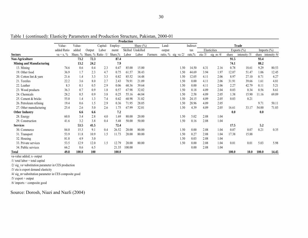
Table 1 shows the sectoral structure of production and trade in the model based on the 2001-02
SAM. Of the 34 sectors, 12 are primary agricultural ones (sectors 1 to 12), and sectors 14 to 18,
which are lightly processed food, are part of the broadly defined agricultural sector in this
8
analysis. The non-agricultural sectors include the mining industry (sector 13), other food (sector
19), manufacturing industries (sectors 20 to 27), energy (sector 28), construction (sector 29), and
5 service sectors (sectors 30 to 34). With these broad sectoral groupings, agriculture produces 27
percent of sectoral value added and 28 percent of the gross value of sectoral output. In the SAM,
it accounts for 12.5 percent of total employment.5
There are 19 household groups in the model. The agricultural-based groups are
categorized by household location (Punjab, Sindh, and other Pakistan) and size of land holdings
(large, medium and small farms, landless small-farm renters, and agricultural workers without
land). In addition, there are four non-farm national aggregates: rural non-farm poor and non-
poor, and urban poor and non-poor. Table 2 shows the 19 households in the SAM and the
corresponding characteristics of these 19 household groups in the HIES.
The structure of consumption varies among household groups. A composite sector of
‘Livestock, cattle and dairy’ has the highest share in the consumption basket, varying from 14
percent in large and medium farms in other Pakistan provinces to 25 percent in agricultural
workers in Punjab. The other major items in the consumption basket are private services (about
14 percent), transport (about 13 percent), wheat milling (from 4 percent among urban non-poor
to 12 percent among agricultural workers in other Pakistan provinces), textile (from 5 percent in
large and medium farms in other Pakistan provinces to 7 percent among agricultural workers in
Punjab and urban poor), other manufacturing (from 1 percent in agricultural workers in Sindh to
10 percent in large and medium farmers in other Pakistan provinces), sugar (from 3 percent in
urban non-poor to 10 percent in agricultural workers in other Pakistan provinces), and fruits and
vegetables (from 4 percent among large and medium farms in Punjab to 7 percent in agricultural
workers in other Pakistan provinces). Commodities with high foreign trade content will be
impacted significantly by changes in trade policies and world prices. This will have varying
effects across household groups because of differences in their consumption bundles.
The sectoral indirect tax structure is presented in table 1. The highest tax rate of 45
percent is on other food whose share in the consumption of households is only about 1 percent.
5 In the SAM, there is also sectoral informal capital. Returns to informal capital may be considered as primarily payment to labor outside of the formal labor market. However, instead of modeling informal capital separately, we aggregated it together with formal capital. There is no significant underestimation of household income, because informal capital is still being paid based on the return to capital. However, this aggregation makes the labor share in agriculture appear relatively low.
9
Indirect taxes are also relatively high on cement and bricks and petroleum refining, which
generally account for less than 1 percent of household consumption directly but affect housing
and transportation costs. The tax rate on cotton lint and yarn is 12 percent and on textiles is zero.
However, since cotton lint and yarn are major inputs into textile production, an increase in the
tax on them will increase the cost of production of textiles. This will affect consumers since the
share of textiles in the consumption basket is about 5 percent.
Sugar has the highest tariff rate of 59 percent (table 3). Another commodity that has high
tariffs, averaging 55 percent, is ‘Livestock, cattle and diary’ which accounts for a large share in
the consumption basket of households. Other agricultural commodities that have high tariffs and
substantial consumption shares are wheat milling and vegetable oil. A few primary agricultural
and light food-processing sectors have low or even negative import tariffs. In contrast, tariffs are
uniformly relatively high across the manufacturing sectors.
Overall, the foreign trade sector in Pakistan is not very large relative to the domestic
sector (table 1). Of the total domestic output, only 10 percent goes to the export market. Of the
total goods and services available in the domestic market, only 15 percent is imported. However,
there are large differences across sectors. Within agriculture, the sectors with the highest share of
their production exported are rice milling IRRI 47 percent, forestry 31 percent, and fishing 24
percent, while it is very small for the rest of the agricultural sectors. Within the non-agricultural
sectors, ‘other food’ has the highest share of production exported at 52 percent, leather is 43
percent, textiles 40 percent, and cotton lint and yarn 27 percent. The textile sector dominates
exports. In the SAM, textiles account a 32 percent of total exports, cotton lint and yarn for 9
percent, and other food 12 percent.
Because of crude oil imports, mining has the highest share of domestic consumption
imported at 81 percent. The share for other manufacturing is 71 percent, for chemicals is 70
percent and for petroleum is 50 percent. Other manufacturing accounts for 54 percent of overall
imports, chemicals 11 percent, and mining and petroleum refining each about 9 percent. Except
for forestry (25 percent) and vegetable oil (20 percent), import intensities for agricultural sectors
are well under 10 percent.
Table 1 includes values of key elasticity parameters in the model: the import substitution
elasticity (sig_m) in the CES composite good function and the production substitution elasticity
10
(sig_va) in the CES value added production function.6 The values of the export demand elasticity
(eta) are the Armington parameters of the global model.
The sources of household income in the model are labor income, capital income, income
from land, and other income (table 4). Other income is composed of foreign remittances,
assumed in the SAM to be distributed proportionately among all households, and dividend
income, which is earned only by urban non-poor households. The sources of income vary across
household groups. Farmers are dependent on income from land, farm labor and capital. Other
rural households depend on income from unskilled labor and capital. About three-fourths of
income of urban poor comes from unskilled labor. Urban non-poor households derive 44 percent
of their income from other income (composed largely of dividend income) and 33 percent from
skilled labor income. According to the Pakistan SAM, it is only the urban non-poor household
group that pays income tax, amounting to 8.4 percent of their income.
Poverty indicators
The overall poverty rate based on the official national poverty line in Pakistan declined from
around 30 percent in the latter 1980s to 26 percent in 1990-91. During these years both urban and
rural poverty declined. However, in 1993-94 rural and urban poverty incidences started to move
in different directions: urban poverty continued to decline while rural poverty began to rise,
thereby widening the gap between urban and rural areas (figure 1). The gap reached its peak in
2001-02, which was largely due to the crippling drought that severely affected agricultural output
that year, together with relatively low international agricultural commodity prices. Almost 70
percent of the people live in rural area and, since the majority of them (40 percent of all
households nationally) depend on agriculture for income, the incidence rural poverty increased to
39 percent that year while urban poverty was stable at 23 percent.
6 We set the sectoral values of the parameter eta in the export demand function equal to the Armington elasticities in the LINKAGE model. The sectoral values of the parameter sig_e in the export supply function and the sectoral values of the parameter sig_m in the import demand function are half the values of eta.
11
There is some disagreement about more-recent estimates of poverty. For 2004-05, the
estimates of the Planning Commission of Pakistan show overall poverty incidence declining
from the peak of 34 percent in 2001-02 to 24 percent in 2004-05. The World Bank (2007)
estimates a smaller decline, to 29 percent. Despite the disparity between these estimates (due
primarily to the inflation factor used in computing the relevant poverty lines), each suggests the
incidence of poverty declined in urban and rural areas in the most recent years and that the gap
between rural and urban poverty rates remains large. The depth of poverty in Pakistan as
indicated by the Foster, Greer and Thorbecke (1994) poverty gap and squared poverty gap also
suggest that the poverty problem is more severe in rural than in urban areas, and that this was
especially true during the 2001-02 drought year (table 5).
Simulations
The first part of this section defines our six policy experiments, while the second part discusses
the results. The experiments use direct tax replacement to hold the government fiscal balance
fixed. The idea is to replace distorting trade taxes with less-distorting income taxes. The fiscal
burden falls on the urban non-poor because, according to the SAM of Pakistan, other household
groups do not pay income tax (table 4). An alternative indirect tax replacement experiment was
also conducted to check the sensitivity of the results to that specification, given that financing a
trade reform is a non-trivial issue from the government’s point of view (Ahmed, Abbas and
Ahmed 2009). In our analysis we separate the effects on the economy of reducing distortions in
the rest of the world and in domestic markets in Pakistan, and evaluate the effects of both on
income inequality and poverty.
Design of the policy experiments
Table 3 shows the sectoral correspondence between the Pakistan model and the global model. It
also shows the sectoral tariff rates and export taxes, which are based where possible on the set of
12
estimates on nominal rate of assistance for Pakistan from Dorosh and Salam (2009). We use
these trade distortions in all our policy experiments. The table also presents changes in the border
import prices under full trade liberalization and agricultural liberalization by the rest of the world
from the global model, and the sectoral export demand shifters calculated on the basis of
equation (2). These are also inputs in the six policy experiments which we conducted, which are
as follows:
• S1A – Full world trade liberalization in all tradable goods sectors by all countries
excluding Pakistan. This experiment uses the results of the global model under full trade
liberalization in table 3. It retains all existing trade distortions in Pakistan.
• S1B – Agricultural price and trade liberalization by all countries excluding Pakistan. This
scenario uses the results of the global model and, as with S1A, all existing distortions in
Pakistan are retained.
• S2A –Full goods trade liberalization in Pakistan carried out unilaterally. All Pakistani
trade distortions are set to zero. There are no changes in the sectoral border export and
import prices or in the export demand shifters because there is no rest-of-world trade
liberalization.
• S2B – Agriculture trade liberalization in Pakistan carried out unilaterally. Thus all
Pakistani distortions in primary agriculture and in lightly processed food are set to zero.
Similar to S2A, there are no changes in the sectoral border export and import prices and
in the export demand shifters because there is no rest-of-world trade liberalization.
• S3A – Full world trade liberalization including Pakistan of all tradable goods. This
combines S1A and S2A.
• S3B – Agricultural world trade liberalization including Pakistan. This combines S1B and
S2B.
In analyzing the results under each of the scenarios, we indicate first the effects on
poverty for the whole of Pakistan, for rural and urban areas, and for major household groups.
The poverty results include changes in poverty incidence and in the depth of poverty as
measured by the poverty gap and squared poverty gap. These poverty effects are traced and
analyzed through the various determining channels: macro, sectoral, commodity and factor
prices, and household income. In estimating the poverty effects, we apply the results on
13
household income and consumer prices for each of the 19 household groups from the CGE
model simulations to the households as classified in the HIES. Each of the CGE simulations
generates a new vector of household income and consumer price for each of the groups, which
we use to compute new sets of poverty indices to compare with the baseline indices.
Simulation results
In this sub-section we present modeling results from the six policy experiments listed in the
previous section sequentially. The discussion continues with some additional results that show
the sensitivity of the core results to changes in the treatment of tax adjustments in the model.
S1A –Trade liberalization by rest-of-world (without Pakistan)
Full trade liberalization abroad, while retaining all existing trade distortions in Pakistan, causes
the overall poverty incidence index to decline by 1.3 percent from its base value as shown in
table 6 (from 31.2 to 30.8). Those at the bottom of the income ladder benefit the most, as
indicated by higher reduction in poverty gap (1.6 percent) and squared poverty gap (1.9 percent).
Among rural households it is the poorest, those in the rural non-farmer group, that benefit the
most.. Thus rural-urban income inequality is lowered in this scenario also.
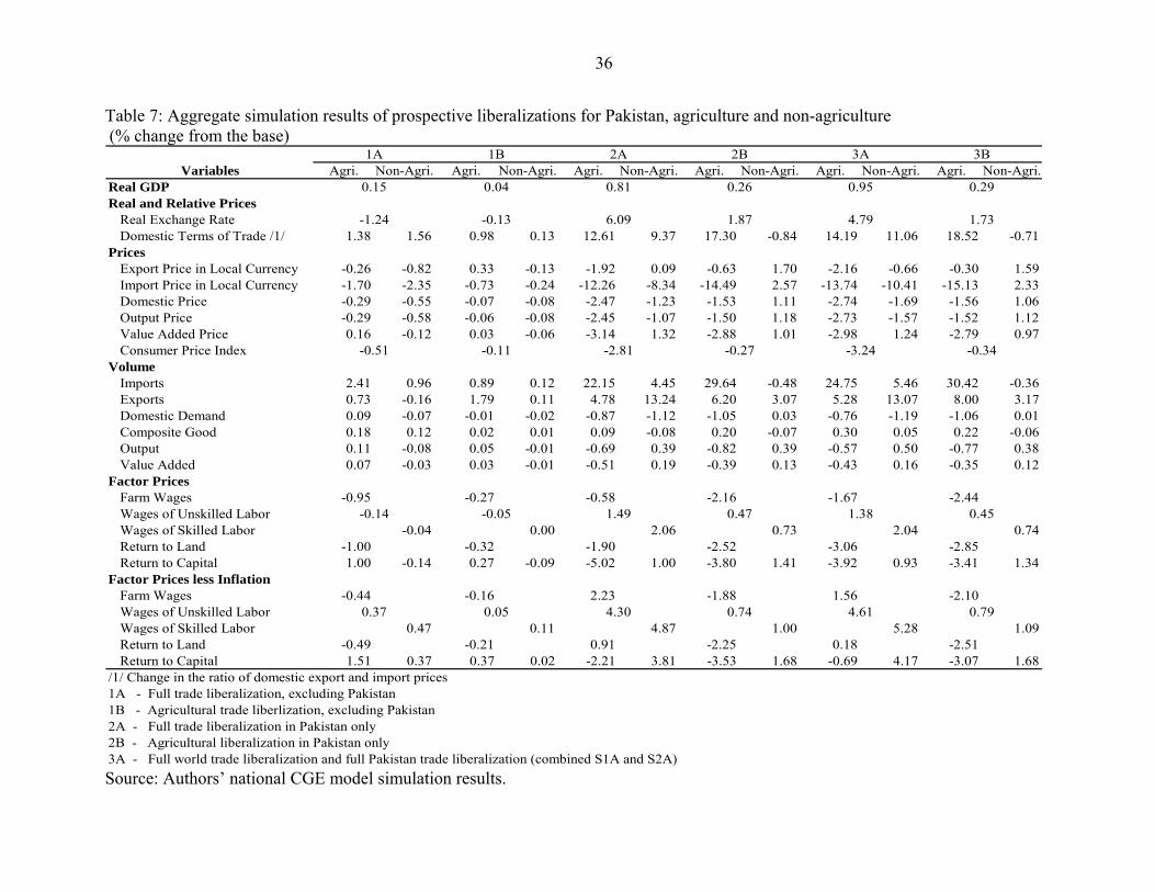
What are the forces that drive these reductions in poverty and income inequality? The
S1A simulation leads to a real exchange rate appreciation7 of 1.24 percent (table 7). The terms of
trade (the ratio of domestic export to import prices) improve by 1.38 percent in agriculture and
by 1.56 percent in non-agriculture. This is because of lower world import prices of some of the
agricultural products as well as most of the non-farm goods (table 3).
The import price of agricultural goods drops by 1.7 percent (table 7) despite increases in
livestock, wheat, vegetable oil and sugar import prices (table 3). This is due to a number of
factors which include the appreciation of the currency, the decline in the border import prices of
7 There is no real exchange rate variable in the model. The real exchange rate is defined as the world price multiplied by the nominal exchange rate divided by the local price, where the world price is trade-weighted world import and export prices and the local price is the sectoral output-weighted local prices.
14
fruits and vegetables and other major crops (table 3), both of which have relatively large import
components (table 1), and the slight reduction in the border import price of forestry which has
high import intensity. The domestic price of farm products declines by 0.3 percent, which is
lower than the drop in import prices. This results in higher imports of agricultural goods (a rise
of 2.4 percent) and a marginal increase in the domestic demand for agriculture of 0.1 percent.
Since demand for both imported and domestic agricultural products increase, domestic
consumption of farm products increases, by 0.2 percent.
Table 3 shows that border import prices of non-agricultural goods decline. This, together
with the appreciation of the exchange rate, reduces the import price of non-agricultural goods by
2.4 percent (table 7). The domestic price of non-agricultural products also declines, by 0.6
percent, which is lower than the decline in the import price. Thus, imports of non-farm products
increases, by 1.0 percent. At the sectoral level , there is a relatively large increase in imports of
‘cotton lint and yarn’, textiles, and leather because of the relatively greater decline in the border
price of these products. Higher imports of non-farm goods reduce marginally the domestic
The export price of farm products declines by 0.3 percent. Since their border prices
increase, the decline is due to the appreciation of the exchange rate. There is a slightly greater
decrease in the domestic price of agricultural products. Thus exports of agriculture improve, by
0.73 percent, and overall output of agriculture increases by 0.11 percent.
The effects on value added, value added prices and factor prices in agriculture are
explained by the changes in sectoral export prices, factor intensities, and import and export
intensities. The overall output price of agriculture declines by 0.29, while the value added price
increases by 0.16 percent. The difference in the sign is due to relatively higher increase in the
value added price of rice milling (2 percent) and vegetable oil (1.7 percent).8 The increase in the
border export price of rice milling of 1.18 percent has larger effects on its value added price
because rice has a high export intensity ratio (table 1). Although the border import price of rice
milling increases more (10.18 percent), it has no effects because of zero imports. The increase in
8 Detailed sectoral results are shown only for scenario S2A (see table 9 below). Detailed comparable sectoral results for the other scenarios are available from the authors on request.
15
the import border price of vegetable oil of 1.78 percent increases its value added price because it
has a high import intensity ratio.
Farm wages and the return to land each decline by around 1.0 percent. This is due to the
decline in the output and value added prices in primary agriculture, which employs farmers and
uses land. The average rate of return to capital in agriculture improves by 1 percent. This is due
to the increase in the value added price of rice milling and vegetable oil. These sectors are
relatively capital intensive, with capital-labor ratios of 3.7 for rice and 6.7 for vegetable oil (table
1). As wage rates increase less than the value added price, returns to capital rise. The return to
capital in these sectors increases by more than 2 percent for rice milling and 1.9 percent for
vegetable oil. The change in the return to capital in livestock and poultry is also positive, but
smaller. The change in the return to capital in the other primary agricultural commodities is
negative.
The decline in the value added price in primary agriculture and in non-agriculture lowers
wages of unskilled labor by 0.14 percent. However, with the increase in the value added price of
rice milling and vegetable oil, the wages of skilled workers decrease by only 0.04 percent. The
average return to capital used in non-agriculture declines by 0.14 percent.
We have also included the results on factor prices that are net of inflation effects. The
overall consumer price index in this experiment decreases by 0.5 percent. Net of inflation effects,
there is a negative result for farm wages and the return to land, but the other factors have positive
net price effects.
All these effects lead to changes in household income, which are summarized in table 8.
The change in nominal income of households is negative across groups except rural non-farm
and rural agricultural workers; the latter because of their heavy reliance on agricultural capital
income (mostly informal capital), as shown in table 4, and the increase in the average return to
capital in agriculture (1 percent, see table 7). However, the consumer prices for each of the
groups decline faster than the drop in nominal income because of the higher reduction in import
prices. Thus, all household groups realize improvement in real income. The highest increases in
real income are for rural non-farmers (0.63 and 0.53 for non-poor and poor, see table 8) and for
agricultural workers in other Pakistan provinces (0.58 percent). This explains the high reduction
in the depth of poverty in rural areas, in particular among rural non-farmers.
16
In sum, this scenario of full trade liberalization by the rest of the world reduces both
poverty and income inequality. It reduces import prices, especially for commodities that have
relatively large shares in the consumption basket of consumers. This translates to declining
consumer prices. It also improves agricultural relative to non-agricultural production because of
improvements in the world price of farm commodities. The poorest in non-farm households in
rural areas benefit the most from the favorable improvement in real wages of unskilled labor and
returns to capital and reduction in consumer prices.
S1B – Agricultural liberalization by rest-of-world
This second experiment incorporates the results of the global model for agricultural liberalization
only by the rest of the world, while retaining all existing trade distortions in Pakistan. Compared
to scenario S1A, border import prices of some of the commodities increase more in the present
scenario. For example, there is a higher increase in border import prices of wheat, livestock,
cotton, rice milling, and sugar (table 3). Furthermore, border import prices of non-agricultural
products increase in the present scenario while they decline in scenario S1A (table 7). Also, for
commodities that have declining border import prices, the drop is relatively higher compared to
scenario S1A. Thus, the increase in the terms of trade for both agriculture and non-agriculture is
lower in this experiment compared to scenario S1A. Also, the increase in the terms of trade in
non-agriculture is significantly lower than in agriculture.
The results in table 6 show that while Pakistan’s overall poverty incidence index declines
marginally, the reduction in poverty is not across the board. Poverty in urban areas declines, but
not all rural households experience a drop in poverty. Rural non-farmers have the highest
poverty reduction, but among farmers and agricultural workers there is a slight increase in
poverty.
What are the factors that drive these poverty results? Import prices of agriculture decline
by 0.7 percent (table 7). This is due to the real exchange rate appreciation of 0.13 percent, and
the reduction in the border price of wheat milling, and fruits and vegetables, which are import-
intensive. There are a number of primary agricultural commodities that have relatively higher
increase in their import prices, but these commodities are not imported. The domestic price of
17
agricultural goods decreases, but by less than the decline in their import price. Thus, imports of
agricultural goods increase, by 0.9 percent.
In non-agriculture, the smaller decline in its domestic prices relative to its import prices
leads to a marginal increase in imports, by 0.12 percent. This increases slightly the domestic
consumption of non-agricultural products.
The increase in the export price of agriculture by 0.33 percent and the decline in its
domestic price by 0.07 percent result in exports rising by 1.8 percent. This increases the overall
output of agriculture slightly, despite the decline in its domestic demand because of higher
imports. But the increase in exports of non-agricultural goods is not quite enough to offset the
decline in domestic demand, so overall output of non-agriculture declines by 0.01 percent.
The difference in the results between the prices of value added and output in agriculture
is due to the varying results across agriculture. The higher increase in the border price of rice
milling leads to a higher value added price, offsetting the decline in the value added price of the
rest of agriculture. The decline in farm wages by 0.27 percent and the return to land by 0.32
percent is due to the decrease in the value added price of primary agriculture. There is an
increase in the return to capital in agriculture by 0.27 percent mainly because of the improvement
in the value added price of rice milling, a sector which has high capital-labor ratio. The decline
in wages of unskilled labor is smaller than farm wages because of the increase in the value added
price of rice milling, which neutralizes much of the falling value added price of the rest of
agriculture and some nonagricultural sectors. Since rice milling employs more skilled labor than
unskilled labor (table 1), the increase in its value added price also offsets the negative effects
coming from the rest of the economy, such that wages of skilled labor do not change.
Net of inflation effects, the impact on factor prices indicate declining farm wages and
return to land. The rest of the factor prices have positive net effects. The nominal income effects
are negative in all household groups (table 8), but smaller than what is generated in scenario
S1A. Consumer prices decline. The decline, however, is not enough to offset the drop in the
nominal income of farmers. But rural non-farmers and urban households enjoy marginal
improvement in real income.
In sum, agricultural liberalization by the rest of the world would generate a marginal
change in the terms of trade that favors agriculture compared to scenario S1A. Furthermore,
18
although overall import prices decline, the drop is much smaller in the present case than in the
previous scenario. This translates to a smaller decline in consumer prices across household
groups which is not enough to offset the drop in nominal income in some groups. These groups –
farmers and agricultural workers – experience a slight increase in poverty. Moreover, given the
small share of agriculture in the overall trade of Pakistan (less than 10 percent, table 1), an
agriculture-only liberalization has much less impact on the Pakistan economy than a
liberalization of all goods trade. Thus, the poverty impact in the present case is significantly less
than in scenario S1A.
S2A – Unilateral liberalization of all goods trade by Pakistan
This third experiment sets to zero all sectoral import tariffs and export taxes in Pakistan and
assumes no changes in policies abroad. Table 6 shows it would generate a significant drop in
poverty, by 5.2 percent overall. There is also a significant reduction in the depth of poverty, with
the poverty gap dropping by 10 percent and the squared poverty gap by 12 percent. However, the
poverty incidence in urban areas increases by 2.3 percent. The detailed results discussed below
show that the urban non-poor suffer a decline in income because of the additional tax burden.
This is the result of the tax replacement where we replaced trade-distorting taxes in Pakistan with
a less-distorting income tax that falls disproportionately on urban non-poor households.9 The rest
of the household groups enjoy higher income and therefore lower poverty. Overall income
inequality is also reduced.
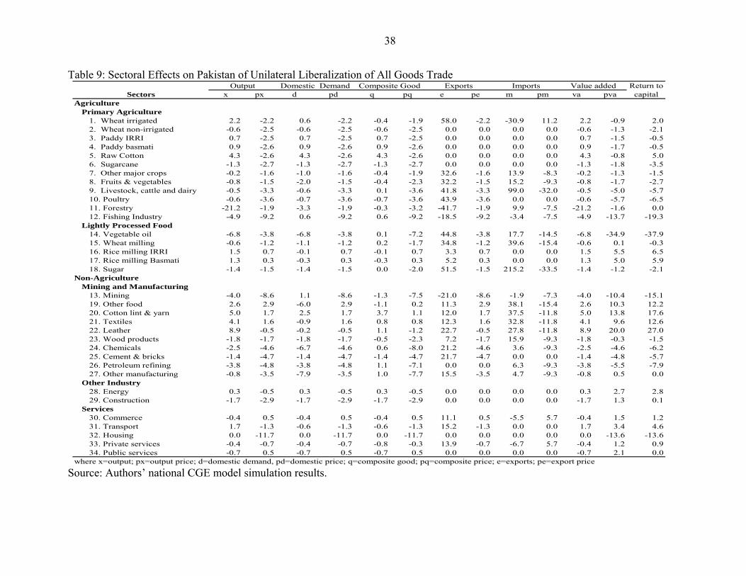
Most of the effects come from the elimination of tariffs, although there are also effects
from the dismantling of export taxes in a number of sectors (table 3). The elimination of tariffs
leads to a substantial reduction in import prices. The greatest reduction is in sugar and livestock,
cattle and dairy, because these sectors have the highest tariff rates. Import prices of vegetable oil,
wheat milling, other food, ‘cotton lint and yarn’ and textiles also decline notably (table 9).
Overall, agriculture has import prices declining by 12 percent, while in non-agriculture they
decline by 8.3 percent (table 7).
9 In the model, the overall government revenue from tariff is Rs154 billion and from export taxes Rs15 billion. Total government revenue is Rs446 billion. The total income of urban non-poor is Rs1.73 trillion.
19
Domestic prices also decline. However, the decline in domestic prices in most of the
sectors is lower than the decline in import prices. Thus, imports in these sectors surge. Imports of
sugar increase by 215 percent, ‘livestock, cattle and dairy’ 99 percent, wheat milling 40 percent,
other food 38 percent, ‘cotton lint and yarn’ 38 percent, textiles 33 percent, and leather 28
percent (table 9). Other sectors have notable increase as well. Overall agriculture has higher
imports by 22 percent, compared with just 4 percent for non-agriculture.
Since world prices are fixed, the decline in prices in Pakistan because of the trade reform
increases its competitiveness.10 There is a real depreciation of the exchange rate of 6.1 percent.
The results in table 9 indicate that, except for forestry and fishing, exports of agriculture
(primary agriculture and lightly processed food) improve. Overall exports of agriculture expand
by 4.8 percent. However, this increase does not offset the displacement effects of the surge in
imports of 22 percent. Thus, overall output of agriculture declines by 0.7 percent. The biggest
reduction is in forestry (21 percent), vegetable oil (7 percent), and fishing (5 percent). However,
there is an improvement in raw cotton production because of the increase in output of ‘cotton lint
and yarn’ and textiles, as discussed below.
In non-agriculture, almost all sectors realize positive growth in exports. Overall exports
of non-agriculture increase by 13 percent. The increase in manufacturing exports is also
substantial, especially in major export items such as ‘cotton lint and yarn’, textile, other food,
and other manufacturing. There is also a notable increase in exports of services such as
commerce, transport, and private services.
For other food, the increase in imports displaces domestic demand by 6 percent.
However, this is offset by the increase in exports; thus its output improves by 2.6 percent and
output price by 2.9 percent. The impact on textiles can be analyzed in relation to the effects on
the ‘cotton lint and yarn’ and raw cotton sectors. The increase in textile imports displaces
domestic demand by 0.9 percent. However, this is offset by the increase in its exports; thus its
output improves by 4.1 percent and output price by 1.6 percent. Since the ‘cotton lint and yarn’
sector supplies materials to the textile sector, the improvement in output of textiles due to higher
exports leads to an improvement in domestic demand for the ‘cotton lint and yarn’, by 2.5
10 In our model, Pakistan is facing a downward sloping world demand curve. Since perfect substitution assumption is imposed between exports and Pakistani domestic sales, the export supply curve for Pakistan is horizontal. The decrease in output prices increases export supply, which shifts the horizontal export supply curve downwards.
20
percent. The increase in both exports and domestic demand for ‘cotton lint and yarn’ leads to a
higher output by 5.0 percent and output price by 1.7 percent, which in turn leads to higher output
of raw cotton by 4.3 percent.
The negative change in the value added price in agriculture leads to lower prices for
factors that are heavily used in agriculture. Wages of farmers decrease by 0.6 percent, returns to
land fall by 1.9 percent, and the average return to agricultural capital falls by 5 percent.
The average output price of non-agriculture decreases by 1.1 percent, but the value added
price improves by 1.3. In table 9, the increase comes from the notable improvement in the value
added price of leather (20 percent), ‘cotton lint and yarn’ (14 percent), other food (10 percent),
textiles (10 percent), and transport (3 percent). Thus, prices of factors used in non-agriculture
improve. Wages of unskilled workers increase by 1.5 percent, skilled labor by 2.1 percent, and
the average return to non-agricultural capital by 1 percent. Furthermore, there is a significant
decline in the consumer price index. Thus net of the inflation effects, factor prices improve
except for the average return to capital used in agriculture.
Nominal income of farmers drops (table 8). As discussed above, this is largely due to
declining wages of farmers, returns to land and the average return to capital in agriculture.
Because of higher wages of workers, nominal incomes of non-farmers improve, except for the
urban non-poor. Incomes of the urban non-poor decline because of the income tax replacement
imposed on this group. However, the decline in consumer price in all groups is significant. This
offsets the decline in nominal income except in urban non-poor.
In sum, all households, except urban non-poor, realize positive increase in real income,
which leads to a significant decline in poverty. The urban poor have the highest increase in
income and the largest drop in the depth of poverty. Again, income inequality is reduced.
S2B – Unilateral agricultural liberalization in Pakistan
This fourth experiment sets to zero just agricultural price distortions in Pakistan11 while retaining
all non-agricultural trade taxes and assuming no changes from the global model. Overall poverty
11 The total tariff revenue from agricultural imports is Rs14.2 billion and farm export tax revenue is Rs 4.3 billion in the baseline.
21
effects are significantly lower in this experiment compared to S2A. Furthermore, there are
differences in the effects across households. Urban households enjoy lower poverty and,
although overall poverty in rural areas declines, large and medium farmers face increasing
poverty.
The results at the macro, sectoral, factor and commodity price levels explain these
poverty effects. At the sectoral level, import prices of agriculture drop by 14 percent (table 7),
the largest declines coming from sugar (36 percent), ‘livestock, cattle and dairy’ (34 percent),
wheat milling (18 percent), and vegetable oil (18 percent).12 There is also a reduction in
domestic prices, but that is significantly smaller than the drop in import prices. Thus imports of
agricultural goods surge by 30 percent.
This agricultural liberalization results in a real exchange rate depreciation. Since tariffs
and subsidies in non-agriculture are retained, their average import prices increase by just 2.6
percent and domestic prices increase by 1.11 percent. Thus, imports of non-agricultural products
decline by 0.5 percent. On the other hand, exports of non-agricultural products improve by 3.1
percent. At the sectoral level, the increase is due to the strong export effect on leather, wood
products, ‘cotton lint and yarn’, and commerce. Since world prices are fixed and domestic and
output prices of non-agriculture are increasing, the increase in its exports is due to the
depreciation of the exchange rate. The increase in exports, together with the marginal increase in
the domestic demand for non-agriculture, leads to an improvement in output by 0.4 percent.
Prices of factors used in agriculture decline. Wages of farmers decrease by 2.2 percent,
return to land by 2.5 percent, and the average return to capital by 3.8 percent. However, prices of
factors heavily used in non-agriculture improve. A similar pattern in factor prices is observed
after netting out the marginal decline in the consumer price index of 0.27 percent.
The nominal income of farmers declines, while the nominal income of non-farmers
improves. The marginal decline in the consumer price index does not offset the decrease in the
nominal income of farmers, especially large and medium farmers. Thus, their real income is
lower. However, non-farmers enjoy higher real incomes, except the urban non-poor for whom
real income falls slightly, again as a result of the tax burden they bear. But the additional tax
burden is not large enough to push them below the poverty line as in S2A, so poverty declines in
12 Detailed sectoral results generated under this scenario are available from the authors upon request.
22
urban areas. Although overall poverty in rural areas declines, large and medium farmers face
increasing poverty because of declining real income.
S3A – Full trade liberalization by Pakistan and the rest-of-world
This fifth experiment combines the trade liberalization in the rest of the world with that in
Pakistan in all sectors. Without going through the detailed results, the effects coming from the
unilateral trade liberalization in Pakistan are larger than the effects from the rest of the world’s
trade liberalization. Their combined impact on both exports and imports is strongly positive.
There is also a large decline in the consumer price index. Factor prices in agriculture decline, but
they improve in non-agriculture. However, net of the inflation effects, the only factor return
decline is in the average return to capital used in agriculture. Nominal incomes of farmers
decline, while nominal incomes for non-farmers improve. The large reduction in the consumer
price index contributes to an increase in real income of all households except the urban non-poor.
This scenario generates the largest reduction in poverty. Another important point worth
highlighting is that while the poverty incidence for the urban non-poor still increases, the
increase is much lower in the present experiment than in scenario S2A.
S3B – Agricultural liberalization by Pakistan and the rest-of-world
This sixth experiment combines the agricultural liberalization of the rest of the world with that in
Pakistan. It turns out that the effects from the reform in Pakistan dominate those from the
agricultural liberalization in the rest of the world. There is also an upward response on imports
and exports, but in agriculture only. The surge in imports of agriculture displaces local
production. This results in lower prices of factors used in agriculture. Factor prices in non-
agriculture increase because the sector remains protected. Therefore, farmers have lower
incomes, while non-farmers benefit.
Sensitivity analysis: indirect versus direct tax replacement
23
The results discussed above are derived using a replacement tax on income. Since the Pakistan SAM
used to calibrate the model has income tax on urban non-poor only (table 4), the direct tax
replacement puts all the burden of financing the trade reform on this group. As an alternative, we
consider in this sub-section indirect taxes to offset losses of government tariff revenue. We focus on
the poverty effects under these two alternative tax replacement schemes in S3A (full trade
liberalization of all goods in the rest-of-world and in Pakistan) and S3B (agricultural liberalization in
the rest-of-world and in Pakistan).
The effects on real income across households are presented in table 10. In S3A where all
sectors are liberalized, changing the tax replacement from direct to indirect completely changes
the results. Under the direct tax replacement all households enjoy higher real income except the
urban non-poor. This tax replacement scheme redistributes income from the urban non-poor to
the rest of the household groups. These household groups benefit from the reduction in consumer
prices and from the redistribution of income from urban non-poor. However, when an indirect
tax replacement is used, consumer prices increase due to the taxes and the burden is shared to all
household groups depending upon their consumption structure. There will be a reduction in
household incomes in most of the groups (all except the three relatively wealthy groups: large
farmers in other Pakistan, rural non-poor, and urban non-poor). Under this tax replacement
scheme, there is a significant increase in domestic prices because of higher indirect taxes.
When trade liberalization is focused on agriculture only under S3B, the income results are
not sensitive to the tax replacement used. This is because net government budget implication of the
elimination of distortions in agriculture is not as large as in non-agriculture. Thus, the impact on
domestic prices through higher indirect tax in the agricultural liberalization case is not as significant
as in the all-goods trade liberalization. In both tax replacement methods, farmers (particularly large
and medium-sized farmers) will be negative affected, while non-farmers will be favorably affected.
However, in the direct tax replacement, urban non-poor will still be negatively affected, but they are
favorably affected under the indirect tax replacement.
Table 11 presents poverty results for this sensitivity analysis. Trade liberalization in all
goods globally under indirect tax replacement in scenario S3A is poverty-increasing. This is
because of the declining real incomes of most groups. This effect comes largely from higher
24
consumer prices as a result of indirect tax replacement. Higher consumer prices wipe out the
gains from higher border export prices, lower border import prices, and lower tariffs.
As for just agricultural liberalization, it entails less of a fiscal burden. Therefore, both the
direct income and the indirect tax replacement generate favorable effects on poverty. In the case
of indirect income tax replacement, although it increases consumer prices, it does not wipe out
the gains from higher border export prices, lower border import prices, and lower trade taxes on
agricultural commodities. Because of the negative effects of the agricultural liberalization on
domestic agriculture in Pakistan, farmers will be hurt, especially large and medium-sized
farmers. But this is a small group in the total population and has the smallest poverty incidence
(23 percent in 2001-02, compared with the poverty incidence of small farmers and agricultural
workers of 37 percent and rural non-farmers of 40 percent).
Summary and policy implications
In this chapter we linked the results of two economic models (the LINKAGE model of the World
Bank and the Pakistan CGE model which we developed) in order to analyze and compare the
poverty effects of trade liberalization abroad with those of unilateral reform by Pakistan. We
conducted six policy experiments: two rest-of-world trade liberalization experiments (full
liberalization that covers all goods sector and agriculture only), two unilateral trade liberalization
cases (all goods and agriculture only), and two combined scenarios. The results are evaluated
under a direct tax replacement on household income, which is paid only by the urban non-poor.
We also examine an alternative tax replacement scheme – an indirect tax replacement on
commodities.
A number of policy insights can be drawn from the simulation results. The impact on the
Pakistan economy and on the extent of its poverty from own-country liberalization is
significantly larger than the effects of rest-of-world trade liberalization. The effect of agricultural
liberalization (both in the rest of the world market and in Pakistan) is considerably smaller than
25
liberalization of all goods trade. This is because of the smaller share of agricultural trade in
overall exports and imports in Pakistan, whose trade is dominated by non-agricultural products.
Income from trade taxes is a major source of revenue for the government. Trade tax
revenue from agricultural commodities is considerably lower than from non-agricultural
products. Thus the elimination of trade taxes on all tradable commodities creates a large dent in
government income and on the fiscal balance. It therefore entails a significant government
demand for tax revenue from other sources. The poverty and income effects of full trade
liberalization greatly depend upon how the tax replacement is implemented. If an additional tax
is imposed on household income to generate funds to finance the reduction in trade taxes in all
sectors, there is a notable decline of consumer prices and a large income redistribution from
urban non-poor to the rest of the household groups. There is therefore a considerable decline in
the poverty incidence, in the depth of poverty, and in income inequality. This is because the
burden of the additional tax falls entirely on the urban non-poor, while the rest of the groups
benefit from higher real factor prices and larger reductions in consumer prices. However, if the
tax replacement is imposed as additional indirect taxes on commodities, consumer prices
increase and eliminate the benefits generated from the reduction in trade distortions. In this case,
poverty increases.
Trade tax revenue from agricultural commodities is considerably lower than from non-
agricultural products. If trade liberalization is focused on agricultural commodities only, the
fiscal re-financing requirement is substantially less. The poverty reduction effects, although
smaller, are robust to the change in tax policy. That is, poverty is reduced under both tax
replacement schemes when only agricultural markets are liberalized.
All these results are derived using a static model. The dynamic impact of trade reform on
capital accumulation from changes in prices has not been accounted for. For example, if the rates
of return to capital are high in sectors where the poor are heavily engaged, it will attract
investment, thereby increasing capital accumulation in and output from those sectors. This would
have favorable implications for poverty. (It is also possible that the results would be reversed and
would therefore generate negative effects on the poor.) Furthermore, the dynamic effects would
also impact on technological progress, movement of farmers’ own labor into non-farm
26
employment, factor and total productivity, and the flow of foreign direct investments. These are
all empirical issues which are relevant topics for further research.
References
Ahmed, V., A. Abbas and S. Ahmer (2009), “Taxation Reforms: A CGE-Microsimulation
Analysis for Pakistan”, Draft Working Paper, Poverty and Economic Policy (PEP)
Network, Quebec.
Anderson K. and E. Valenzuela (2008),”Estimates of Global Distortions to Agricultural
Incentives, 1955 to 2007”, World Bank, Washington DC, October, accessible at
www.worldbank.org/agdistortions.
Anderson, K., E. Valenzuela and D. van der Mensbrugghe (2010), “Global Poverty Effects of
Agricultural and Trade Policies Using the Linkage Model”, Ch. 2 in K. Anderson, J.
Cockburn and W. Martin (eds.), Agricultural Price Distortions, Inequality and Poverty,
London: Palgrave Macmillan and Washington DC: World Bank.
Cororaton, B.C. and D. Orden (2008), Pakistan’s Cotton and Textile Sectors: Intersectoral
Linkages and Effects on Rural and Urban Poverty, IFPRI Research Report 158,
Washington DC: International Food Policy Research Institute.
Decaluwé, B., J. Dumot and V. Robichaud (2000), “MIMAP Training Session on CGE
Modeling. Volume II: Basic CGE Models”. Available at: www.pep-net.org (“MPIA”,
“training material”)
Dorosh, P. (2005), “Wheat Markets and Pricing in Pakistan: Political Economy and Policy
Options”, Wheat Policy Note, South Asia Rural Development Unit, World Bank,
Washington DC.
Dorosh, P., M.K. Niazi and H. Nazli (2004), “A Social Accounting Matrix for Pakistan, 2001-02:
Methodology and Results”, PIDE Working Paper No 2006:9. Islamabad: Pakistan
bThe official figures for 1993-94 indicate overall poverty in Pakistan was above urban and rural poverty incidence (http://www.accountancy.com.pk/docs/Economic_Survey_2002-03.pdf. Chapter 4, Table 4.1, page 3) Source: Ministry of Finance (2003) and, for 2004-05 estimates, World Bank (2007).
Total 49.8 100.0 100 100.0 100.0 10.0 100.0 14.45va-value added; x- output/1/ total labor ÷ total capital /2/ sig_va=substitution parameter in CES production/3/ eta is export demand elasticity/4/ sig_m=substitution parameter in CES composite good/5/ export ÷ output/6/ imports ÷ composite good
ProductionShare (%) Trade
Elasticities Exports (%) Imports (%)
Source: Dorosh, Niazi and Nazli (2004)
31
Table 2: Household Categories in Pakistan 2001-02 Social Accounting Matrix (SAM) 2001-02 Household Integrated Economic Survey (HIES)
Large farmers - Sindh Landowners with more than 50 acreas - Punjab - Other PakistanMedium farmers - Sindh Landowners with more than 12.5 acres but less than 50 acreas - Punjab - Other PakistanSmall farmers - Sindh Landowners with more than 0 acres but less than 12.5 acreas - Punjab - Other PakistanSmall farm renters and landless - Sindh No landholdings, but rented land for farm activities - Punjab - Other PakistanRural agri. workers and landless - Sindh No landholdings, agricultural workers - Punjab - Other PakistanRural non-farm - non-poor Rural non-poor, non-farmers and non-agricultural workers - poor Rural poor, non-farmers and non-agricultural workersUrban - non-poor Urban non-poor - poor Urban poorThree Major Provinces: (1) Punjab; (2) Sindh; and (3) Other Pakistan - Balochistan, North-West Frontier Province,Source: Dorosh, Niazi and Nazli (2004) and Federal Bureau of Statistics (2003).
32
Table 3: Parameters and exogenous demand and price shocks on Pakistan due to liberalization in the rest of the world LINKAGE Model
/1/ This is the trade weighted average of cattle sheep, other livestock, and dairy in the LINKAGE model/2/ In equation 2, this is a=(1+0.01*p)(1+0.01*q)^(1/ESUBM); where p is export price change, q export volume change; and ESBUM Arimington elasticity,
Pakistan CGE Model Trade Distortions Full Trade Lib., excl. Pakistan Agri. Trade Lib., excl. Pakistan
Source: Linkage model simulations (see Anderson, Valenzuela and van der Mensbrugghe 2010).
33
Table 4: Sources of Household Income and Income Taxes, Pakistan, 2001-02
Total Per Capita DirectHouseholds mil Rs '000 Rs '000 % dist. Farm Unskilled Skilled K Land Other tax, %
Factor PricesFarm Wages -0.95 -0.27 -0.58 -2.16 -1.67 -2.44Wages of Unskilled LaborWages of Skilled Labor -0.04 0.00 2.06 0.73 2.04 0.74Return to Land -1.00 -0.32 -1.90 -2.52 -3.06 -2.85Return to Capital 1.00 -0.14 0.27 -0.09 -5.02 1.00 -3.80 1.41 -3.92 0.93 -3.41 1.34
Factor Prices less InflationFarm Wages -0.44 -0.16 2.23 -1.88 1.56 -2.10Wages of Unskilled LaborWages of Skilled Labor 0.47 0.11 4.87 1.00 5.28 1.09Return to Land -0.49 -0.21 0.91 -2.25 0.18 -2.51Return to Capital 1.51 0.37 0.37 0.02 -2.21 3.81 -3.53 1.68 -0.69 4.17 -3.07 1.68
/1/ Change in the ratio of domestic export and import prices1A - Full trade liberalization, excluding Pakistan1B - Agricultural trade liberlization, excluding Pakistan2A - Full trade liberalization in Pakistan only2B - Agricultural liberalization in Pakistan only3A - Full world trade liberalization and full Pakistan trade liberalization (combined S1A and S2A)
0.95 0.29
1A 1B 2B2A
0.15 0.04 0.81 0.26
0.74 0.79
-2.81 -0.27 -3.24 -0.34
4.61
0.47 1.38 0.45-0.14
0.37 0.05 4.30
-0.05 1.49
4.79 1.73
3A 3B
-0.51 -0.11
-1.24 -0.13 6.09 1.87
Source: Authors’ national CGE model simulation results.
Imports Value addedOutput Domestic Demand Composite Good Exports
Source: Authors’ national CGE model simulation results.
39
Table 10: Sensitivity Analysis of Household Welfare Effects to Type of Tax Replacement, Pakistan
Source: Authors’ national CGE model simulation results.
40
Table 11: Sensitivity Analysis of Poverty Effects to Type of Tax Replacement, Pakistan P0=poverty headcount; P1=poverty gap; P2=poverty severity3A - Full world trade liberalization and full Pakistan trade liberalization (combined 1A and 2A)3B - Agriculture trade liberalization and agriculture Paksitan trade liberalization (combined 1B and 2B)
Source: Authors’ national CGE model simulation results.