This article investigates whether, and to what degree, poverty is linked to other types of welfare problems and, in larger perspective, whether the situation can be understood in terms of social exclusion. Two different measures of poverty – income poverty and deprivation poverty – and 17 indicators of welfare problems were used in the analysis. It was shown that income poverty was rather weakly related to other types of welfare problems, i.e. the most commonly used measure of poverty seems to discriminate a section of the population that does not suffer from the kinds of problems we usually assume that poverty causes.
This article investigates whether, and to what degree, povertyis linked to other types of welfare problems and, in largerperspective, whether the situation can be understood in termsof social exclusion. Two different measures of poverty –income poverty and deprivation poverty – and 17 indicatorsof welfare problems were used in the analysis. It was shownthat income poverty was rather weakly related to other typesof welfare problems, i.e. the most commonly used measure ofpoverty seems to discriminate a section of the population thatdoes not suffer from the kinds of problems we usually assumethat poverty causes. Deprivation poverty, identifying thosewho most often had to forgo consumption of goods andservices, did correlate strongly with other types of welfareproblems. Hence, people living under poor conditions dosuffer from welfare problems even though this section of thepopulation is not always captured by income povertymeasures. The final analysis showed that the types of welfareproblems that were most likely to cluster were deprivationpoverty, economic precariousness, unemployment, psychologicalstrain and health problems. Whether these types ofaccumulated welfare problems, from a theoretical perspective,can be seen as indicators of social exclusion is more doubtful.
Poverty, welfare problems and social exclusionHalleröd & Larsson
Poverty, welfare problems and social exclusion
Key words: poverty, social exclusion, welfare, deprivation, socialpolicy, marginalisation
Björn Halleröd, Department of Sociology, Umeå University,SwedenE-mail: [email protected]
Accepted for publication December 8, 2006
The Amsterdam treaty places the fight against povertyand social exclusion at the centre of the EuropeanUnion’s (EU) social agenda. But what is the relationshipbetween poverty and social exclusion? Can we andshould we distinguish these concepts from each other,or is the label just a tautology? Is the fight againstpoverty one thing and the fight against social exclusionanother, or do they essentially constitute a single battle?To answer these questions, we need to conceptuallydistinguish poverty from its causes and consequencesand empirically investigate whether, and how, povertyis linked to other types of welfare problems and, in theend, whether this situation can be understood in termsof social exclusion.
In this article, we will study the consequences ofpoverty, focusing mainly on how poverty is related to arange of other welfare problems such as unemployment,health, psychological distress, victimisation etc. Thepurpose is also to analyse whether, and how, differentwelfare problems are related to not only poverty butalso to each other. In a wider perspective, the analysisis linked to the discussion about social exclusion, aphenomenon often understood as accumulated welfareproblems, i.e. a situation in which a single individual is
suffering from several different welfare problems at thesame time (cf. Gallie, Paugam & Jacobs, 2003; Hills,Le Grand & Pichud, 2002).
The article is organised in the following way: thefollowing section deals with the theoretical definition ofpoverty and how to distinguish poverty from other typesof welfare problems and social exclusion. Thereafter,measurements of poverty and welfare problems arediscussed. The empirical analyses are presented in thepenultimate section, followed by the discussion andconclusions.
Poverty and social exclusion
Why is it important to identify the poor and to takeaction against poverty? The commonsensical answer isthat poor people suffer from malnutrition, lack ofshelter, ill health, exclusion from an ordinary lifestylein society etc., and that such a situation is unacceptable.In a way, one could say that this broad picture ofpoverty is correct because if the poor do not suffer froma wide range of problems, why should we bother aboutpoverty? The problem from an analytic perspective isthat inclusion of almost every unwanted condition in
the theoretical definition of poverty makes it impossibleto analyse the causes and consequences of poverty. Italso becomes more or less unfeasible to distinguishpoverty from other concepts such as social exclusion.We therefore need a theoretical definition of povertythat focuses on the inability to make ends meet. Thatis,
the poor are those who, due to insufficient access toeconomic resources, have an unacceptably low levelof consumption of goods and services
. The importantconsequence of this kind of definition is that, forexample, malnutrition
per se
is not poverty; it is causedby poverty only if it is lack of economic resources thatmakes it impossible for a person to acquire food. Thefact that malnutrition is most often a poverty problemdoes not mean that it is always a poverty problem.Consider, for example, anorexia, a condition in whichmalnutrition is not caused by poverty. Similarly, badhealth is, in many cases, unrelated to poverty. It is onlya consequence of poverty if it is caused by an inabilityto buy adequate food, provide for shelter or pay forhealthcare. The relationship between poverty and othertypes of welfare problems is further complicated by thefact that welfare problems often cause poverty. Thereis plenty of evidence to show that unemployment isproblematic even if the unemployed person is protectedfrom poverty (cf. Nordenmark, 1999; Strandh, 2000).But it is, of course, also reasonable to argue thatunemployment often causes poverty. It is also easyto see that health problems can cause poverty bypreventing people from earning a living. Disentanglingcauses and effects at the individual level is, to put itmildly, empirically complicated, and the process isprobably best understood as either a ‘vicious circle’leading to an accumulation of welfare problems intoa situation of social exclusion, or a ‘good circle’ out ofsocial exclusion. An important step in facilitating ourunderstanding of these ‘circles’ is to discover whether,and how, poverty and other welfare problems areinterlinked with each other at one point in time. Thismeans that we must first distinguish different types ofwelfare problems and then empirically check whetherthey form a cluster of accumulated welfare problems.In this perspective, poverty should be seen as just onewelfare problem conceptualised as lack of economicresources.
There are a number of studies showing that welfareproblems do cluster (Bask, 2005; Erikson & Tåhlin,1987; Fløtten, 2005; Halleröd, 1991; Halleröd &Heikkilä, 1999; Tham 1994). Recently, Bradshaw andFinch (2003) examined the degree to which threedifferent measures of poverty were related to differentaspects of social exclusion in Britain. In line withearlier findings (cf. Berthoud, Bryan & Bardasi, 2004;Halleröd 1991, 1995, 2000; Kangas & Ritakallio, 1998),they found that the overlap between different povertymeasures was fairly limited, i.e. different measures
tended to identify different individuals as poor and thatdifferent measures of poverty were distributeddifferently in the population. The unique contributionof Bradshaw and Finch is that they also demonstratedthat different measures of poverty relate differently todifferent indicators of welfare problems. Thecontribution of this article is that it takes previousanalyses of the relationship between welfare problemsa step further and studies in detail whether welfareproblems are related and, if so, what kind of welfareproblems cluster and how such a cluster is related topoverty. Lastly, we will approach the issue of whetheran empirically observed cluster of welfare problems canbe reasonably understood in terms of social exclusion.
Three hypothetical outcomes regarding the relationshipbetween poverty and other types of welfare problemscan be put forward:
1. Poverty is not related to other welfare problems, aresult implying that poverty in today’s Sweden,because it apparently does not have any welfareconsequences, is more or less a quasi-problem.
2. We find a cluster of related welfare problems, but thecluster is unrelated to poverty. The conclusion in thiscase would be that accumulation of welfare problemsis an empirical fact clearly distinguished from povertyand that poverty is still to be viewed as a quasi-problem.
3. Poverty is related to a range of welfare problems.Poverty, thus, can be viewed as a serious problemand keeping people out of poverty would appear tobe an important goal for social policy. This outcomealso makes it reasonable to view the fight againstpoverty and the fight against social exclusion as asingle battle.
Data and measurements
The data are from Statistics Sweden’s annual Survey ofLiving Conditions from 1998 (ULF98) and are basedon face-to-face interviews with a random sample of theSwedish population aged 16–84 years. The randomsample contains 7,400 individuals, and the totalworking sample amounts to 5,732, which givesa response rate of 77.5 per cent. The working sampleis limited to respondents aged 20–74 years, which givesa working sample consisting of 4,941 cases. ULF98contains a large number of welfare indicators and aunique set of questions regarding consumption of goodsand services that facilitates a so-called consensualmeasurement of poverty introduced by Mack andLansley back in the early 1980s.
Poverty measures: operationalisation
We will employ two measurements of poverty: incomepoverty and deprivation poverty. Income poverty is
measured in accordance with the conventional EUmeasurement of relative poverty, i.e. those who live ina household with an equivalent disposable income thatis below 60 per cent of the median household incomeare defined as poor. Income data are gathered from theincome register and represent the households’ disposableafter-tax income from all registered sources. Thedisposable income is adjusted to household size usingan equivalence scale developed by the SwedishNational Board of Health and Welfare (StatisticsSweden [SCB], 2003).
1
Deprivation poverty is measured using a weighteddeprivation index (WDI) (Halleröd, Gordon, Larsson &Ritakallio, 2006). The index measures inability to
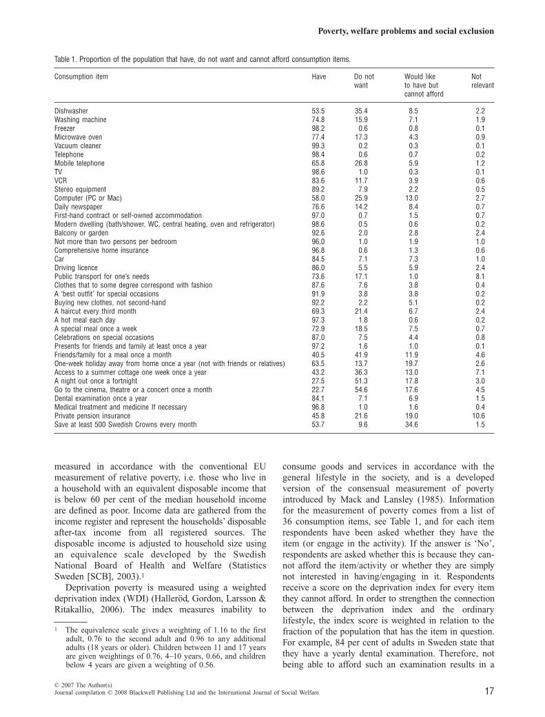
consume goods and services in accordance with thegeneral lifestyle in the society, and is a developedversion of the consensual measurement of povertyintroduced by Mack and Lansley (1985). Informationfor the measurement of poverty comes from a list of36 consumption items, see Table 1, and for each itemrespondents have been asked whether they have theitem (or engage in the activity). If the answer is ‘No’,respondents are asked whether this is because they can-not afford the item/activity or whether they are simplynot interested in having/engaging in it. Respondentsreceive a score on the deprivation index for every itemthey cannot afford. In order to strengthen the connectionbetween the deprivation index and the ordinarylifestyle, the index score is weighted in relation to thefraction of the population that has the item in question.For example, 84 per cent of adults in Sweden state thatthey have a yearly dental examination. Therefore, notbeing able to afford such an examination results in a
1
The equivalence scale gives a weighting of 1.16 to the firstadult, 0.76 to the second adult and 0.96 to any additionaladults (18 years or older). Children between 11 and 17 yearsare given weightings of 0.76, 4–10 years, 0.66, and childrenbelow 4 years are given a weighting of 0.56.
Table 1. Proportion of the population that have, do not want and cannot afford consumption items.
Consumption item Have Do not want
Would like to have but cannot afford
Not relevant
Dishwasher 53.5 35.4 8.5 2.2Washing machine 74.8 15.9 7.1 1.9Freezer 98.2 0.6 0.8 0.1Microwave oven 77.4 17.3 4.3 0.9Vacuum cleaner 99.3 0.2 0.3 0.1Telephone 98.4 0.6 0.7 0.2Mobile telephone 65.8 26.8 5.9 1.2TV 98.6 1.0 0.3 0.1VCR 83.6 11.7 3.9 0.6Stereo equipment 89.2 7.9 2.2 0.5Computer (PC or Mac) 58.0 25.9 13.0 2.7Daily newspaper 76.6 14.2 8.4 0.7First-hand contract or self-owned accommodation 97.0 0.7 1.5 0.7Modern dwelling (bath/shower, WC, central heating, oven and refrigerator) 98.6 0.5 0.6 0.2Balcony or garden 92.6 2.0 2.8 2.4Not more than two persons per bedroom 96.0 1.0 1.9 1.0Comprehensive home insurance 96.8 0.6 1.3 0.6Car 84.5 7.1 7.3 1.0Driving licence 86.0 5.5 5.9 2.4Public transport for one’s needs 73.6 17.1 1.0 8.1Clothes that to some degree correspond with fashion 87.6 7.6 3.8 0.4A ‘best outfit’ for special occasions 91.9 3.8 3.8 0.2Buying new clothes, not second-hand 92.2 2.2 5.1 0.2A haircut every third month 69.3 21.4 6.7 2.4A hot meal each day 97.3 1.8 0.6 0.2A special meal once a week 72.9 18.5 7.5 0.7Celebrations on special occasions 87.0 7.5 4.4 0.8Presents for friends and family at least once a year 97.2 1.6 1.0 0.1Friends/family for a meal once a month 40.5 41.9 11.9 4.6One-week holiday away from home once a year (not with friends or relatives) 63.5 13.7 19.7 2.6Access to a summer cottage one week once a year 43.2 36.3 13.0 7.1A night out once a fortnight 27.5 51.3 17.8 3.0Go to the cinema, theatre or a concert once a month 22.7 54.6 17.6 4.5Dental examination once a year 84.1 7.1 6.9 1.5Medical treatment and medicine If necessary 96.8 1.0 1.6 0.4Private pension insurance 45.8 21.6 19.0 10.6Save at least 500 Swedish Crowns every month 53.7 9.6 34.6 1.5
score of 0.841 on the deprivation index. However, theseweights are only average. It is likely that consumptionpatterns are different in different sections of the population.Calculation of the index takes into account two suchdifferences (for a more detailed discussion see Halleröd1995; Halleröd et al., 2006). First, it is acknowledgedthat consumption patterns differ across age groups.Second, it is also recognised that families with childrenhave needs that families without children do not have.Construction of the deprivation index implies that:
a) People who cannot afford consumption items/activitiesthat most people have/engage in are suffering frommore deprivation than are people who cannot affordthings/activities that very few people have/engage in.
b) An elderly person is not suffering from deprivationif he/she cannot afford things/activities that onlyyoung people have/engage in, and vice versa.
c) A person who lives in a household without childrendoes not score on the index if he/she lacks thingsthat, practically, only households with children have.
Formally, the WDI is calculated in the following way:
I =
Σγ
i
(P =
α
+
β
i
χ
1
+
β
i
χ
2
)
where
γ
i
tells us whether individual i wants but cannotafford item
γ
, P is the weight for item
γ
, estimated asthe probability for individual i to have
γ
given
χ
1
(his/her age), and
χ
2
(whether or not she/he is living in ahousehold with children). As is the case for mostdeprivation of this type, the reliability is very high, with aCronbach alpha score of 0.86. As can be seen in Table 1,10.4 per cent of the population is counted as incomepoor. We use this figure to define a likewise arbitrarypoverty line for the deprivation index. Counting thosewith a deprivation score above 4.36 as poor will resultin a corresponding poverty figure of 10.4. In the bestof all worlds, the same 10.4 per cent is defined as poorby both measures. However, we do not live in such aworld, and only 2 per cent are actually income poor anddeprivation poor at the same time. Thus, there are goodreasons for using both measures in the following analysis.
Welfare problems: indicators of social exclusion
To analyse how different welfare problems relate toeach other, in addition to the poverty measures, 17indicators of different welfare problems will be used.These indicators range from aspects that tap into areasoften discussed in relation to social exclusion, such asneighbourhood characteristics, unemployment and lackof political involvement, but more individual characteristicssuch as health conditions, loneliness and psychologicaldistress are also included.
Lack of political activity is measured in the followingway. Respondents are asked whether they have ‘at anytime tried to do something about any deficiency or
inaccuracy in your municipality’, and whether they inthat case had: contacted any civil servant or otherrepresentatives, written a letter to the press or an articlein a newspaper, signed any appeal, participated in anydemonstration or done anything else to express theirview? In addition to this, a more general question wasalso posed: ‘Considering political issues overall, notonly here in the municipality, have you at any time:written a letter to the press or an article in a newspaper,signed any appeal or participated in any demonstration’.Those who answered ‘No’ to all eight questions aredefined as politically inactive. This indicator issupplemented with a measure that identifies those whodid not vote in the latest general election.
We do not have access to information about housingenvironment as such, i.e. we lack information related tospecific areas. However, we do have information fromthe respondents that, at least to some degree, can beseen as indicators of area features at the same time asthey also indicate individual welfare problems. Toindicate what we will call ‘socially disorganised areas’,a concept originally used by Shaw and McKay (1969),we use a set of variables that indicate whether therespondent is living in a suburban area in a larger townor city in Sweden. The indicator shows that the respondentis living in a town with at least 90,000 inhabitants, thatthe accommodation is rented and located in a block offlats with at least three floors and that the respondentstates that damage to housing facilities is common.If all four of these criteria are met, the housing area isdefined as socially disorganised (Nilsson & Estrada,2004). An additional housing variable measures whetherthe respondent thinks that his/her dwelling is too small,adequate or too big. The answer ‘too small’ is used asan, admittedly subjective, indicator of crowded housing.
We also measure victimisation and concerns aboutcrime. One variable measures whether the respondenthas been exposed to any type of theft or propertydamage during the previous 12 months. A second variablemeasures whether the respondent, during the previous12 months, has been exposed to violence or threats ofviolence. A third variable captures whether the respondent,again during the past 12 months, has refrained fromgoing out during the evening due to fears of beingassaulted in any way or whether the respondent isworried about theft and damage to his/her own dwelling.
Health, psychological strain and, to some degree,health behaviour are measured using six differentindicators. Health problems are measured via a questionthat asks whether the respondent suffers from any long-standing illness or handicap that negatively impacts onhis/her ability to work or perform daily activities. Addi-tional indicators of health condition and psychologicaldistress are based on questions about occurrence, overthe previous two weeks, of sleeping problems, recurrentheadaches or migraine and anxiety, worry or anguish.
Lastly, we also include two important health predictors:smoking and obesity. Smokers are those who smokeevery day, and people are defined as obese if their bodymass index exceeds 30.
Loneliness is measured using a subjective indicator.Respondents are confronted with five statements andare asked to pick the one that best describes theirsituation. The statements are:
1) I basically never feel lonely.2) Sure, sometimes I feel lonely, but I don’t consider it
to be a problem.3) Sometimes I feel lonely and I wish that I could see
other people more often.4) I very often feel lonely.5) I almost always feel lonely.
People are considered to be lonely if they agree withstatement 3, 4 or 5.
Human capital is indicated by education, and avariable is created that discriminates those who haveprimary compulsory education as their highest level ofeducation. Economic vulnerability is a condition that,in one sense, is almost synonymous with poverty. Wewill argue, however, that lack of a cash margin in thehousehold economy, measured as the inability to raise14,000 SEK (Swedish Crowns) within a week, is anadditional indicator of economic vulnerability that may ormay not coincide with poverty. We will, lastly, measureunemployment. The measure we have chosen capturesthose who, during the previous five years, have beenunemployed for a total period of at least 12 months.
The distribution of welfare problem indicators is shownin Table 2. The most common problems are political
inactivity and long-standing illness. Seven of theindicators are experienced by less than 10 per cent ofthe population, whereas nine of the welfare problemsare experienced by between 10 and 40 per cent of thepopulation.
Results
Table 3 shows the proportion among income poor,deprivation poor and non-poor that experience any ofthe 17 additional welfare problems. Eleven of the17 welfare problems are significantly more commonamong the income poor than among the non-poor, whileall 17 welfare problems are significantly more commonamong the deprivation poor than among the non-poor.In 14 cases, there is also a significant difference betweenthe income poor and the deprivation poor. In all thesecases, incidences of welfare problems are higher amongthe deprivation poor. Thus, poverty seems to be closelyrelated to other types of welfare problems, somethingthat is emphasised when we move from the commonlyused income measure to a deprivation-based measure ofpoverty.
Estimations of the bivariate association betweendifferent welfare problems are displayed in Table 4. Tomore clearly see the pattern of associations between thevariables, in Figure 1 we have used the coefficients fromTable 4 as input values to a multi-dimensional scalinganalysis, estimating Euclidian distances in order toconstruct two-dimensional visualisations of the results.The fit of this two-dimensional model is not particularlygood; the so-called stress value is 0.17, indicating thatthe data have a structure that is too complex to be
Table 2. Basic statistics on poverty and social exclusion indicators.
N Per cent
Income poor 510 10.4Deprivation poor 490 10.4Income poor and deprivation poor 93 2.0Not poor 3,837 81.3Did not vote 490 10.6Politically inactive 2,046 41.8Victimisation: crime 1,475 30.1Victimisation: violence 333 6.9Worried about crime 451 9.3Disorganised area 297 6.2Crowded housing 725 15.0Health problem 1,978 40.4Headache 742 15.3Anxiety 872 18.0Sleep 961 19.8Obesity 406 8.5Smoking 1,026 21.1Loneliness 480 9.9Low education 1,057 21.6Lack of cash margin 755 15.6Unemployed 466 9.7
Table 3. Prevalence of welfare problems among income poor, deprivation poor and non-poor (per cent).
* Indicates significance in relation to the non-poor: * p < 0.05; ** p < 0.001; *** p < 0.0001. Bold figures indicate significant difference (p < 0.001) between income poor and deprivation poor.
represented by two dimensions. The map neverthelessgives an informative first overview of how welfareproblems are related to each other. Looking first at thepoverty measures, we see that income poverty is placedfar out to the left of the map. Income poverty is, in fact,one of the variables used here that has the weakest totalrelationship to other kinds of welfare problems, and itis also one of the variables that are significantly relatedto the fewest of the other variables (see Table 4). In thisanalysis, economic poverty shares this peripheralposition with lack of political involvement, crowdedhousing, exposure to property crime and obesity. Forthese four indicators, we can find convincing argumentsas to why they are only weakly related to other typesof welfare problems. The way we measure lack ofpolitical involvement discriminates everyone who hasnot made an active effort to act in a political matter.Thus, people might score on this indicator because theyare content with political decisions, not because theylack a political voice. Crowded housing is moreaffected by household composition than by socialexclusion; it is mainly households with children thatreport lack of housing space. Exposure to propertycrime is a function not only of the vulnerability relatedto social exclusion, but also of the extent to whichpeople have properties that are worth stealing (Larsson,2006). Obesity was included as an indicator of healthhazards and is also an indicator that relates strongly tolong-standing health problems, but, as the resultsindicate, obesity is only loosely associated with otherwelfare problems. Therefore, we have few reasons to be
concerned about the weak correlation between thesefour indicators and other welfare problems. It is, ofcourse, more disturbing that the most commonly usedpoverty measure discriminates a section of thepopulation that is only marginally connected to otherwelfare problems.
Poverty measured in terms of deprivation is placedalmost exactly in the middle of the map. Furtherinvestigation of Table 4 shows that deprivation povertyis the only variable to be positively and significantlycorrelated with all the other variables, and the correla-tions are generally high. Around deprivation poverty wesee a cluster of welfare problems that are stronglyinterlinked and also closely connected to deprivationpoverty. There is a cluster of welfare problems that tellsus that deprivation poverty often coincides with long-standing health problems, anxiety and sleeping pro-blems and, also, loneliness. Deprivation poverty, to amuch higher degree than economic poverty, is alsoassociated with lack of an economic buffer. Living in asocially disorganised area is also connected to depriva-tion poverty, as are concerns about being subjected tocrime. The connection between unemployment anddeprivation is also relatively strong.
The analysis presented in Table 4 and Figure 1 notonly tells us that deprivation poverty seems to be moreclosely connected to other types of welfare problemsthan is income poverty, but also gives us a picture ofthe kinds of problems that most likely make up the corecauses and consequences of poverty, i.e. inability toconsume in accordance with the ordinary lifestyle,
Figure 1. Relationship between income poverty and welfare problems. Multi-dimensional scaling based on Kendall tau_b estimates.
unemployment, living in disorganised areas, sufferingfrom social and psychological strain and also, to somedegree, health problems.
Latent class analysis
The analysis above clearly shows that some types ofwelfare problems are more closely interlinked thanothers. It also reveals that the data are too complex tobe properly represented by two dimensions. To find outwhether there are distinct clusters of welfare problems,a series of latent class analyses was conducted. Theanalysis identifies clusters that group together personswho share common characteristics. The model classifiescases into clusters based on membership probabilities.It offers a wide range of indicators of model fit and alsoa decomposed measure, making it possible to evaluatethe contribution of single indicators. In the first setof analyses, models were specified that included all19 welfare indicators (including the poverty measures).The number of clusters was allowed to vary from 1 to10 in order to determine a stage at which an additionalincrease in the number of clusters did not lead to asubstantial improvement of the model fit. Theimprovement of the model is indicated by the chi-square-based likelihood value (L
2
). The L
2
value forone cluster model tells us how much total residualvariance there is left to explain in the model, variancethat theoretically can be explained by additionalclusters. These analyses showed that when the one-cluster model was relaxed to a three-cluster model, theL
2
value decreased by 20 per cent, from 12,431 for theone-cluster model to 9,887 for the three-cluster model.Thereafter, the L
2
value decreased only marginally foreach extra cluster added to the model. However, theoverall performance of the three-cluster model wasquite poor, as indicated by the very modest decrease inL
2
value. This was due to the fact that several of themanifest welfare problem variables were only weaklyassociated with the three latent clusters at the same timeas these welfare problems were only weakly related toeach other, i.e. they did not form separate clusters whenthe model was relaxed to allow more than three clusters.To find a simpler model containing only variables thatwere more closely related to each other, we reduced thenumber of variables in the model. Looking at theresiduals for each variable and the Entrypo-R
2
indicating to what degree the latent cluster variablepredicted the manifest variable outcome, we started todelete from the model the manifest variables that weremost weakly associated with the three clusters,beginning with the one with the lowest R
2
value (whichhappened to be income poverty). After the removal ofa variable, we checked the model fit, as indicated by theBIC variable (the L
2
value adjusted for model complexity),calculated as BIC
the removal actually improved the model. In the end,we ended up with eight manifest measures of welfareproblems that were all relatively strongly associatedwith the three clusters: long-standing health problems,headaches, anxiety, sleeping problems, loneliness, lackof cash margin, unemployment and deprivation poverty.
For these eight variables, a series of analyses wasconducted in which the number of clusters was allowedto vary between 1 and 5. Allowing for only two clustersresulted in a considerable improvement of the model.The L
2
value decreased from 2,445 to 704. Allowingfor an additional third cluster decreased the L
2
value to369. A fourth cluster only marginally improved themodel, at the same time as making a substantialinterpretation of the clusters increasingly difficult. Thefirst row of Table 5 shows the size of the three clustersestimated from the modal values. Here we can see that71 per cent of the population ended up in the non-problematic group, i.e. they have low probabilities ofscoring on any of the eight welfare problems. Almost20 per cent belong to cluster 2. The risk of belongingto this cluster is basically determined by the health-related indicators, while unemployment, lack of cashmargin and deprivation poverty played a minor role.The third cluster was the smallest, and around 10 percent of the population was estimated to belong to thiscluster. The difference between cluster 2 and cluster 3is that cluster 3 combines high probability of beingunemployed and having economic problems with highprobabilities of having health impairments, anxiety,sleeping problems and headaches. Hence, cluster 3groups together people with a high probability ofscoring on all eight welfare problems.
In a final analysis, we used a multinominal logisticregression model to estimate the risk for people indifferent sections of the population to end up in cluster2 or cluster 3. The independent variables are: equivalentdisposable income, age (both these variables aresupplemented with a quadratic term) and socio-economic class as indicated by Statistic Sweden’s
socioeconomic code, which in turn closely resemblesthe well-known EGP schema (Erikson & Goldthorpe,1993). Seven different classes were distinguished (seeTable 6). People currently not employed or self-employedwere classified according to their previous labour marketposition or, as the second option, according to theirspouse’s labour market position. If neither of theseoptions were available, the categorisation ‘unclassified’was used. Also included are household type and gender.The purpose of this analysis was not to make athorough search for the most important determinates ofaccumulated welfare problems or to test a particulartheoretical model. It was simply a test of the degree towhich a number of important stratification variables arerelated to the cluster we obtained and therefore alsohelps us to interpret the clusters in a meaningful way.
Looking first at cluster 2, there is no relationshipbetween income and cluster probability. The probabilityincreases with age, but is only weakly related to socialclass. There is a slight risk increase among those wholive in households without children and among singleparents compared with couples with children. Lastly, itis revealed that the odds ratio is significantly lower formen. The analysis confirms that cluster 2 is basically ahealth cluster that is more or less unrelated to economiccircumstances. Cluster 3 is different. Here we see aclose connection to income: the higher the income, thelower the cluster probability. The significant estimatefor the quadratic term also tells us that the risk ofbelonging to cluster 3 decreases with increasing speedas income increases. This is, of course, not a surprise,as deprivation poverty and lack of cash margin arestrongly related to the cluster. However, the result isinteresting when seen against the above resultsregarding income poverty, as it basically indicates thataccumulation of welfare problems is a low income
Table 5. Latent class analysis: cluster size, classification probabilities and model fit.
Cluster 1 Cluster 2 Cluster 3
Health problem 0.30 0.68 0.51Headache 0.07 0.37 0.30Anxiety 0.05 0.49 0.42Sleeplessness 0.06 0.57 0.36Loneliness 0.04 0.18 0.29Lack of cash margin 0.06 0.15 0.72Unemployment 0.06 0.07 0.35Deprivation poverty 0.02 0.05 0.75
Equivalent disposable household income 0.996 0.717***Quadratic term 1.000 0.981***Age 1.016*** 0.984**Quadratic term 1.000 0.998***
Class: Higher white collar as ref groupUnskilled blue collar 1.521** 5.258***Skilled blue collar 1.239 4.004***Lower white collar 1.141 3.155**Middle white collar 0.874 1.814Self-employed 1.055 0.805Others 1.393 4.824***
Household: Cohabiting with child(ren) as ref group Cohabiting without children 1.264* 1.354Single adult without children 1.567*** 3.639***Single adult with children 1.673* 5.158***
problem, but not so much an income poverty problem.Relating this outcome to earlier findings about therelationship between income distribution anddeprivation, the most likely explanation is that theprevalence of income measurement errors is largest atthe bottom end of the income distribution. Therefore,we find among the income poor a rather large fractionnot suffering from deprivation with regard toconsumption of goods and services and, likewise, notparticularly exposed to other types of welfare problems(Halleröd, 1997; Halleröd et al., 2006). To furtherunderpin this conclusion, in Figure 2 the probabilityscore for cluster 3 is plotted against disposable income.The estimates are derived from a logistic regressionmodel that includes disposable income and thequadratic term of disposable income. Here we can seethat the probability is highest among people living in alow-income household and that the probability peaksjust below the poverty line. However, among thoseliving in households with extremely low incomes, theprobability risk decreases. Because it is unlikely that theextremely poor are better off than people living inhouseholds closer to the poverty line, it is difficult toimagine that the result is caused by anything other thanmeasurement problems. A recent comparative analysisindicates that this problem is not exclusive to Sweden,as the same phenomenon has been seen in two otherstudied countries: Finland and Great Britain (Hallerödet al., 2006).
The risk of belonging to cluster 3 is highest amongyoung people and decreases with age with increasingspeed, which is shown by the negative coefficient forthe quadratic age term. There are large differencesbetween different classes, and the odds ratio forunskilled workers is five times greater than that forhigher white-collar workers. The same is true of peopleliving in single adult households with children. Also,
single adults without children have a substantiallyhigher risk of falling into cluster 3. The risk forinclusion in cluster 3 is also lower for men than forwomen. Thus, the analysis supports the interpretationthat clusters 2 and 3 are essentially different.
Conclusions and discussion
The questions addressed here concern the relationshipbetween poverty and a wide range of welfare problemsand, in a wider perspective, the relationship betweenpoverty and social exclusion. The analyses wereconducted in several steps. Our data allowed us to useboth an income-based measure of poverty definingthose with an income below 60 per cent of the medianincome as poor, and a deprivation-based measuredefining those who most often have to forgoconsumption of goods and services as poor. In additionto these two poverty measures, we also distinguished 17indicators of welfare problems that covered integrationin the political process, neighbourhood conditions,housing conditions, health impairments, anxiety andpsychological distress, health hazards, socialintegration, educational marginalisation, unemploymentand economic vulnerability. In the first step of theanalysis, the interrelationships between poverty and all17 welfare problems were estimated. The analysisshowed that poverty measured as deprivation wassignificantly related to each of the other 17 welfareproblems. However, the income poverty measure wasrelated to only 11 of the welfare problems, and theserelationships were generally comparably weak. In fact,the analysis revealed that income poverty was one ofthe most peripheral of all welfare problems. Thus,knowing that someone has an income below 60 per centof the median income does not tell us with any certaintythat she/he actually suffers from welfare problems, and
Figure 2. Estimated probability of belonging to cluster 3 by household equivalent income.
we can certainly not claim that fighting income poverty,as we are able to identify it, will also contributesignificantly to the fight against other forms of welfareproblems. These results are in line with much of theprevious research in the area (Berthoud et al., 2004;Bradshaw & Finch, 2003; Callan, Nolan & Whelan,1993; Halleröd, 1995; van den Bosch, 2001). However,we cannot draw the conclusion that poverty in today’sSweden is a trivial problem. Those who were identifiedas deprivation poor, i.e. those most unable to consumegoods and services in accordance with the generallifestyle in contemporary Sweden, suffered greatly froman accumulation of welfare problems.
What our analysis shows is that the traditional wayof measuring poverty as low income is problematicbecause of a series of unsolved measurement problemsthat are most likely to affect the lower tail of the incomedistribution. To estimate poverty correctly based onincome data, we of course need correct data on people’saccess to economic resources from the start. We can berelatively certain that income data are problematic fromthis point of view. Income from the black economy,income in kind, savings, non-monetary resources etc.,cloud the connection between income data andconsumption (Behrendt, 2002; Halleröd, 2000). Otherproblems concern the difficulties in identifying thecorrect household unit and the fact that equivalencescales adjust for household size in a rather crude way.Time is another important factor. A short poverty spellmight be mitigated by the use of savings, and theacquisition of clothes, furniture and other kinds ofseldom-consumed items can be postponed (Berthoudet al., 2004; Breen & Moisio, 2004; Gordon, 2005;Layte & Whelan, 2003). The assumption of equalsharing within the household has been increasinglyquestioned during recent decades (Nyman, 2002; Pahl,1989; Vogler & Pahl, 1994).
In the next step of the analysis, latent class analysiswas used to distinguish a set of closely related welfareproblems. In the end, a three-cluster model was derived,based on eight welfare problems. These were long-standing health problems, recurring headaches, anxiety,sleeping problems, loneliness, unemployment, lack ofcash margin and poverty measured as deprivation. Acluster that comprises about 10 per cent of thepopulation scored high on all eight of these variables.Thus, when people in today’s Sweden suffer from arange of welfare problems, these are the types ofproblems most likely to affect them. The resultspresented here are based on cross-sectional data anddo not prove any causality between welfare problems.Thus, we cannot know whether poverty causes healthproblems or whether health problems cause poverty. Arealistic guess is that causality goes in both directions.In our opinion, further investigation of the causalitybetween welfare problems is of great importance to social
policy discussions. However, the analysis does give anindication of what it is like to be poor in Sweden today.
The results presented here indicate that fightingpoverty and social exclusion largely constitutes thesame battle if we accept two basic assumptions. Thefirst is that we need to measure poverty in a moreaccurate way than is usually the case, i.e. we cannot relyon available income data only. Second, the approach tosocial exclusion that we have applied is largely datadriven. Based on our analysis, we can argue that thesocially excluded in today’s Sweden are poor andunemployed and that they also experience healthproblems, loneliness and psychological distress. Thesocially excluded, thus, are excluded from the labourmarket and from ordinary consumption of goods andservices, and in addition they suffer from moreindividual problems such as ill health and psychologicaldistress. However, aspects that are often looked upon ascentral in the debate on social exclusion – such asexclusion from the political arena and education system,and spatial segregation – seem to be only weakly relatedto each other and to the core problems identified in thisstudy, making the relation between poverty and socialexclusion less straightforward than is usually assumed.Our hope is that the findings presented here can serveas fuel not only for continued empirical analysis ofsocial exclusion, but also for the theoretical debate onthe concept of social exclusion.
Regarding further empirical studies, we see twoimportant issues. First, the kind of analysis conductedhere needs to be extended to include other countries.The EU-SILC (Survey of Income and Living Con-ditions) database will hopefully provide the informationnecessary for such an analysis. Second, we need tounderstand the social mechanisms that link poverty anddifferent kinds of welfare, i.e. we need to understandthe process of social exclusion and, of course, also theprocesses that lead to social inclusion. This is, on alllevels, a challenging endeavour for social science.
References
Bask M (2005). Welfare problems and social exclusion amongimmigrants in Sweden.
European Sociological Review
21:73–89.
Behrendt C (2002).
At the Margins of the Welfare State
.Aldershot, Ashgate.
Berthoud R, Bryan M, Bardasi E (2004).
The dynamics ofdeprivation: the relationship between income and materialdeprivation over time
. Report No. 219, Department for Workand Pensions, London.
Bradshaw J, Finch N (2003). Overlaps in Dimensions of Poverty.
Journal of Social Policy
32: 513–525.Breen R, Moisio P (2004). Poverty Dynamics Corrected for
Measurement Errors.
Journal of Economic Inequality
2: 171–191.
Callan T, Nolan B, Whelan CT (1993). Resources, Deprivationand the Measurement of Poverty.
and social exclusion: Is there a vicious circle of socialexclusion?
European Societies
5: 1–32.Gordon D (2005). The Concept and Measurement of Poverty.
In: Pantazis C, Levitas R, eds.
Poverty and Social Exclusionin Britain: The Millennium Survey
. Bristol, The Policy Press.Halleröd B (1991).
Den svenska fattigdomen
[The SwedishPoverty]. Lund, Arkiv.
Halleröd B (1995). The Truly Poor: Indirect and DirectMeasurement of Consensual Poverty in Sweden.
Journal ofEuropean Social Policy
5: 111–129.Halleröd B (1997). Fattigdom och materiell deprivation: En
empirisk analys [Poverty and Deprivation: An EmpiricalAnalysis]. In: Vogel J, Häll L, eds.
Välfärd och ojämlikhet i20-års perspektiv 1975–1995
. Örebro, StatistiskaCentralbyrån.
Halleröd B (2000). Socialbidragstagande och fattigdom [SocialAssistance and Poverty]. In: Puide A, ed.
Socialbidrag iforskning och i praktik.
Göteborg, Gothia.Halleröd B, Gordon D, Larsson D, Ritakallio V-M (2006).
Relative Deprivation – A Comparative Analysis of Britain,Finland and Sweden.
Journal of European Social Policy
16:328–345.
Halleröd B, Heikkilä M (1999). Poverty and Social Exclusion inthe Nordic Countries. In: Kautto M, Fritzell J, Hvinden B,Kvist J, Uusitalo H, eds.
Nordic Social Policy. London,Routledge.
Hills J, Le Grand J, Piachud D (2002). Understanding socialexclusion. Oxford, Oxford University Press.
Kangas O, Ritakallio V-M (1998). Different Methods – DifferentResults? Approaches to Multidimensional Poverty. In:Andreß HJ, ed. Empirical Poverty Research in a ComparativePerspective. Aldershot, Ashgate.
Larsson D (2006). Exposure to crime as a consequence ofpoverty. Umeå, Umeå University, Department of Sociology.
Layte R, Whelan CT (2003). Moving in and out of poverty –The impact of welfare regimes on poverty dynamics in theEU. European Societies 5: 167–191.
Mack J, Lansley S (1985). Poor Britain. London, George Allen& Unwin Ltd.
Nilsson A, Estrada F (2004). Exposure to threatening and violentbehaviour among single mothers – the significance oflifestyle, neighbourhood and welfare situation. BritishJournal of Criminology 44: 168–187.
Nordenmark M (1999). Unemployment, Employment Commitmentand Well-Being. Umeå, Umeå University, Department ofSociology.
Nyman C (2002). Mine, yours or ours. Umeå, Umeå University,Department of Sociology.
Pahl J (1989). Money and Marriage. London, MacmillanEducation Ltd.
Shaw CR, McKay HD (1969). Juvenile delinquency and urbanareas; a study of rates of delinquency in relation todifferential characteristics of local communities in Americancities. Chicago, University of Chicago Press.
Strandh M (2000). Varying Unemployment Experience? TheEconomy and Mental Well-Being. Umeå, Department ofSociology, Umeå University.
Tham H (1994). Ökar marginaliseringen i Sverige? [IsMarginalization in Sweden Increasing?]. In: Fritzell J,Lundberg O, eds. Vardagens villkor [Conditions of daily life].Stockholm, Brombergs.
van den Bosch K (2001). Identifying the Poor. Aldershot, Ashgate.Vogler C, Pahl J (1994). Money, Power and Inequality within
Marriage. The Sociological Review 42: 263–288.
ISBN 978-92-79-16351-7
Price (excluding VAT) in Luxembourg: EUR 20
Income and living conditions in Europe Edited by Anthony B. Atkinson and Eric Marlier
This book is about the incomes and living standards of the people of Europe. It treats employment, income inequality and poverty, housing, health, education, deprivation and social exclusion. The reader will learn about many of the social issues confronting Europe. How much income poverty is there in Europe? Is inequality increasing? Does a job guarantee escape from income poverty? How is Europe’s welfare state coping with the economic crisis? The book is a timely contribution to the Europe 2020 Agenda as it explores ‘the new landscape of EU targets’ and the implications for monitoring at EU and national levels.
Evidence about these important issues comes primarily from the EU Statistics on Income and Living Conditions (EU-SILC), which represents a powerful instrument for the comparative analysis of the economic and social state of the EU as well as a growing number of non-EU European countries. The book is the result of the Network for the analysis of EU-SILC (Net-SILC), which was funded by the Statistical Office of the EU (Eurostat). Net-SILC was an ambitious initiative that brought together official statisticians responsible for producing statistics and researchers who use these data.
By analysing statistics to examine the living conditions of European citizens we can learn how to produce more and better figures, and also how to develop evidence-based policies for better achieving social objectives.
http://ec.europa.eu/eurostat KS-31-10-555-EN
-C
Income and living conditions in Europe
Edited
by Anthony B. A
tkinson and Eric M
arlier
S t a t i s t i c a l b o o k s
Edited by Anthony B. Atkinson and Eric Marlier
Income and living conditions in Europe
S t a t i s t i c a l b o o k s
Edited by Anthony B. Atkinson and Eric Marlier
Income and living conditions in Europe
logos essentiels EN - FR- DE
Fichier indd et pdf dans : /tampon revue/office/AO_10023/repasse/logos/logos-EN-FR-DE
EN
FR
DE
Europe Direct is a service to help you find answers to your questions about the European Union.
Freephone number (*):
00 800 6 7 8 9 10 11(*) Certain mobile telephone operators do not allow access to
00 800 numbers or these calls may be billed.
More information on the European Union is available on the Internet (http://europa.eu).
Cataloguing data can be found at the end of this publication.
Luxembourg: Publications Office of the European Union, 2010
ISBN 978-92-79-16351-7doi:10.2785/53320Cat. No KS-31-10- -EN-C
Theme: Population and social conditionsCollection: Statistical books
Printed on elemental chlorine-free bleached PaPer (ECf)
555
Income and living conditions in Europeeurostat 3
forewordThe European Commission attaches utmost importance to tackling problems of poverty and exclusion and developing policies targeting the most disadvantaged of our citizens. One of the headline targets in the Europe 2020 Strategy for Jobs and Growth is promoting social inclusion, in particular through the reduction of poverty, by aiming to reduce the number of people at risk of poverty and excluded from full participation in work and society. The “Platform Against Poverty” under the Europe 2020 Strategy will bring together European action for vulnerable groups such as children and old people. Last but not least, 2010 has been the European Year for Combating Poverty and Social Exclusion. We must make sure that the most vulnerable are not left behind.
The publication that you have in front of you is an integral part of this political agenda. The social indicators are essential to monitor progress towards our common goals. They play a key role in shaping our economic and social policies. We need reliable data for a high quality statistical analysis. Given that social well-being has many dimensions and its measurement goes well beyond the level of GDP, the improvement of the quality of statistics and their coverage is even more important.
The publication is a significant contribution as it explores ‘the new landscape of EU targets’ and the implications for monitoring at EU and national levels. The Europe 2020 agenda, in setting a social inclusion target, has highlighted three dimensions of poverty and exclusion. It is also essential, however, that Member States – and the EU as a whole – continue to monitor performance according to the full set of commonly agreed social indicators underpinning EU coordination and cooperation in the social field.
“Income and Living Conditions in Europe” is the result of the work of a Network established by Eurostat of statisticians responsible for producing statistics and researchers who use these data, which focuses on the contribution of the EU Statistics on Income and Living Conditions (EU-SILC). The book, therefore, is not just for policy-makers, nor just for statisticians. It will interest all those concerned with the social dimension of Europe. The reader will learn about how the citizens of Europe earn their living, about their living arrangements, their social participation, and about the ways in which their incomes are affected by taxes and transfers. The book gives a clear picture of many social problems confronting Europe and of the distributional effects of social and labour policies.
The success of Europe 2020 with a truly social dimension will depend on real ownership at the European, national and local levels. Fighting poverty is a shared responsibility – one where everyone has a role to play. Providing a better understanding of these issues is a concrete step that will help the Commission and Member State governments to achieve their objectives.
José Manuel Barroso
President of the European Commission
Income and living conditions in Europe eurostat4
(1) http://www.stat.gov.pl/eusilc/index.htm.
Eurostat is the Statistical Office of the European Communities. Its mission is to pro-vide the European Union with high-quality statistical information. For that purpose, it gathers and analyses figures from the national statistical offices across Europe and provides comparable and harmonised data for the European Union to use in the defi-nition, implementation and analysis of Community policies. Its statistical products and services are also of great value to Europe’s business community, professional organisations, academics, librarians, NGOs, the media and citizens.
Eurostat's publications programme consists of several collections: News releases provide recent information on the Euro-Indicators and on social,
economic, regional, agricultural or environmental topics. Statistical books are larger A4 publications with statistical data and analysis. Pocketbooks are free of charge publications aiming to give users a set of basic fig-
ures on a specific topic. Statistics in focus provides updated summaries of the main results of surveys, stud-
ies and statistical analysis. Data in focus present the most recent statistics with methodological notes. Methodologies and working papers are technical publications for statistical
experts working in a particular field.Eurostat publications can be ordered via the EU Bookshop at http://bookshop.europa.eu.
All publications are also downloadable free of charge in PDF format from the Eurostat website http://ec.europa.eu/eurostat. Furthermore, Eurostat’s databases are freely available there, as are tables with the most frequently used and demanded short- and long-term indicators.
Eurostat has set up with the members of the ‘European statistical system’ (ESS) a network of user support centres which exist in nearly all Member States as well as in some EFTA countries. Their mission is to provide help and guidance to Internet users of European statistical data. Contact details for this support network can be found on Eurostat Internet site.
Eurostat is the Statistical Office of the European Communities. Its mission is to provide the European Union with high-quality statistical information. For that purpose, it gathers and analyses figures from the national statistical offices across Europe and provides comparable and harmonised data for the European Union to use in the definition, implementation and analysis of Community policies. Its statistical products and services are also of great value to Europe’s business community, professional organisations, academics, librarians, NGOs, the media and citizens.
Eurostat’s publications programme consists of several collections:
• News releases provide recent information on the Euro-Indicators and on social, economic, regional, agricultural or environmental topics.
• Statistical books are larger A4 publications with statistical data and analysis.
• Pocketbooks are free of charge publications aiming to give users a set of basic figures on a specific topic.
• Statistics in focus provides updated summaries of the main results of surveys, studies and statistical analysis.
• Data in focus present the most recent statistics with methodological notes.
• Methodologies and working papers are technical publications for statistical experts working in a particular field.
Eurostat publications can be ordered via the EU Bookshop at http://bookshop.europa.eu.
All publications are also downloadable free of charge in PDF format from the Eurostat website http://ec.europa.eu/eurostat. Furthermore, Eurostat’s databases are freely available there, as are tables with the most frequently used and demanded shortand long-term indicators.
Eurostat has set up with the members of the ‘European statistical system’ (ESS) a network of user support centres which exist in nearly all Member States as well as in some EFTA countries. Their mission is to provide help and guidance to Internet users of European statistical data. Contact details for this support network can be found on Eurostat Internet site.
Acknowledgements by editorsThe Network for the Analysis of EU-SILC (Net-SILC) was an ambitious 18-partner Network bringing together expertise from both data producers (directly involved in the collection of EU-SILC data) and data users. It was established in response to a call for applications by the Statistical Office of the European Union (Eurostat) in 2008. We would like to thank Eurostat not only for funding Net-SILC but also for their very active and efficient support throughout the project. We would also like to give a particular word of thanks to Gara Rojas González and Pascal Wolff for their important assistance in the final editing of this book. Their detailed comments and suggestions have been extremely useful.
This book represents a major output from the Network for the Analysis of EU-SILC (Net-SILC). However, not all of the scientific work produced by the Network could be included in it. More technical material, and the output from the more methodological Net-SILC work packages, are available in the series ‘Eurostat methodologies and working papers’. We wish to thank all the Net-SILC members and the institutions they belong to for their contribution to the project (for a list of Net-SILC members, see Appendix 1).
The initial Net-SILC findings were presented at the international conference on Comparative EU Statistics on Income and Living Conditions (Warsaw, 25-26 March 2010) (1) which was organised jointly by Eurostat and the Net-SILC network. We would like to thank the Central Statistical Office of Poland for kindly hosting the event. Special thanks also go to Olympia Bover, Conchita D’Ambrosio, André Decoster, Stephen Jenkins, John Micklewright and Brian Nolan for discussing so thoroughly the papers at the conference and also for guiding us in our editorial decisions related to this book. Both this book and the Net-SILC Working Papers published by Eurostat have benefited from their input.
Isabelle Bouvy and Begoña Levices have provided invaluable secretarial and bibliographical help.
It should be stressed that the book does not represent in any way the views of Eurostat, the European Commission or the European Union. It also does not represent in any way the views of the persons and bodies thanked above. All the authors have written in a strictly personal capacity, not as representatives of any Government or official body. Thus they have been free to express their own views and to take full responsibility for the judgments made about past and current policy and for the recommendations for future policy.
A.B. Atkinson (Nuffield College and London School of Economics, United Kingdom)
E. Marlier (CEPS/INSTEAD Research Institute, Luxembourg)
Income and living conditions in Europeeurostat 7
Table of Contents Foreword ............................................................................................................................................................3
Acknowledgements by editors ........................................................................................................................5Table of Contents ..............................................................................................................................................7List of tables, figures and boxes ....................................................................................................................15
Living conditions in Europe and the 1. Europe 2020 agenda (Anthony B. Atkinson and Eric Marlier) ............................................................................................211.1 Introduction .....................................................................................................................................221.2 Outline of the contents ...................................................................................................................231.3 Summary of main lessons for EU-SILC .......................................................................................281.4 EU-SILC in the new landscape of EU targets ..............................................................................30
1.4.1 Implications for monitoring at EU level.........................................................................311.4.2 Implications for EU social indicators .............................................................................321.4.3 Implications for monitoring at Member State level ......................................................331.4.4 An EU minimum income for children ...........................................................................33
Investing in statistics: 2. EU-SILC (Pascal Wolff, Fabienne Montaigne and Gara Rojas González) ......................................................372.1 Introduction .....................................................................................................................................38
2.1.1 A brief history ....................................................................................................................382.1.2 Policy context .....................................................................................................................38
2.2 The EU-SILC instrument and its governance ..............................................................................402.2.1 Scope and geographical coverage ....................................................................................402.2.2 Main characteristics of EU-SILC ....................................................................................402.2.3 Legal basis ..........................................................................................................................412.2.4 Common guidelines ..........................................................................................................41
2.3 Methodological framework ............................................................................................................422.3.1 Contents of EU-SILC ........................................................................................................422.3.2 Income concept .................................................................................................................422.3.3 Sample requirements ........................................................................................................442.3.4 Tracing rules ......................................................................................................................46
2.4 Information on quality ....................................................................................................................462.4.1 Some comparability issues ...............................................................................................462.4.2 Quality reports ...................................................................................................................51
2.5 Data and indicators .........................................................................................................................522.5.1 Data access .........................................................................................................................522.5.2 Indicators computation ....................................................................................................52
2.6 The way forward ..............................................................................................................................532.6.1 Improvement of timeliness and geographical coverage ..............................................532.6.2 Methodological and data improvements .......................................................................532.6.3 Coherence with other sources .........................................................................................542.6.4 Data linking .......................................................................................................................542.6.5 Revision of the EU-SILC legal basis ..............................................................................55
Data accuracy in 3. EU-SILC (Vijay Verma and Gianni Betti) ...........................................................573.1 Introduction: a description of errors in survey data ...................................................................58
3.1.1 A typology of errors ..........................................................................................................583.1.2 Errors in measurement .....................................................................................................583.1.3 Errors in estimation ..........................................................................................................593.1.4 Item non-response ...........................................................................................................613.1.5 Comparability ....................................................................................................................61
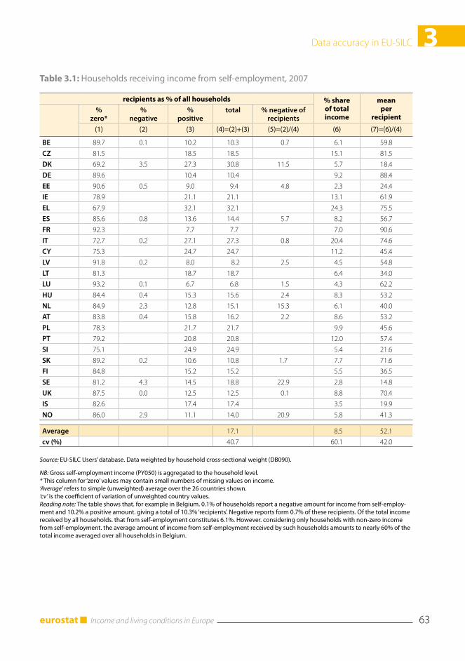
3.2 Conceptual and measurement errors ............................................................................................623.2.1 Reporting of negative and zero values for income components .................................623.2.2 Total household gross and disposable income (HY010, HY020) ...............................623.2.3 Total household disposable income
before social transfers (HY022, HY023) .........................................................................643.2.4 The importance of uniform procedures for achieving comparability ........................65
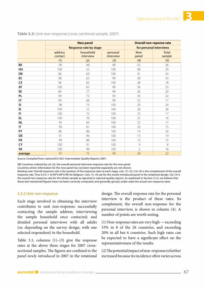
3.3 Non-response in EU-SILC .............................................................................................................663.3.1 A framework ......................................................................................................................663.3.2 Unit non-response.............................................................................................................673.3.3 Within-household (‘partial unit’) non-response ...........................................................683.3.4 Item non-response ............................................................................................................69
3.4 Sampling error .................................................................................................................................713.4.1 Jackknife Repeated Replication (JRR) for variance estimation ...................................713.4.2 Defining sample structure: ‘computational’ strata and PSUs ......................................723.4.3 Analysis of design effects in EU-SILC ............................................................................733.4.4 Illustrative estimates of variance and of design effect and its components ...............75
3.5 Concluding remarks .......................................................................................................................753.5.1 Diverse sources of non-sampling errors in EU-SILC ...................................................753.5.2 Improving the potential for assessment of data quality in EU-SILC ..........................76
Household structure in the EU 4. (Maria Iacovou and Alexandra Skew) ..........................................794.1 Introduction .....................................................................................................................................80
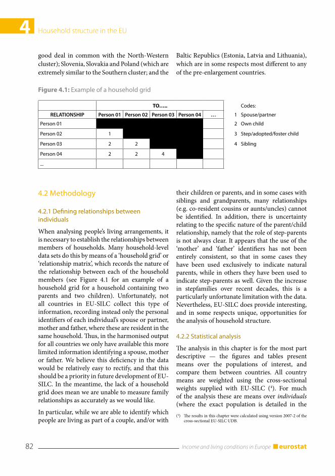
4.1.1 Countries and groups of countries .................................................................................814.2 Methodology ....................................................................................................................................82
4.2.1 Defining relationships between individuals ..................................................................824.2.2 Statistical analysis ..............................................................................................................82
4.3 Household composition..................................................................................................................834.4 Children ............................................................................................................................................854.5 Young adults .....................................................................................................................................884.6 Partnerships: cohabitationand marriage ......................................................................................894.7 Older people .....................................................................................................................................924.8 Synthesising the differences: factor analysis ................................................................................944.9 Conclusions ......................................................................................................................................97References ...............................................................................................................................................98
Income poverty and income inequality 5. (Anthony B. Atkinson, Eric Marlier, Fabienne Montaigne and Anne Reinstadler) ...................................................................................1015.1 Introduction ...................................................................................................................................102
5.1.1 Aim of this chapter ..........................................................................................................1025.1.2 Role of EU-SILC ..............................................................................................................102
Income and living conditions in Europeeurostat 9
5.2 Income poverty/inequality across countries and comparison with international sources..........................................................................................................104
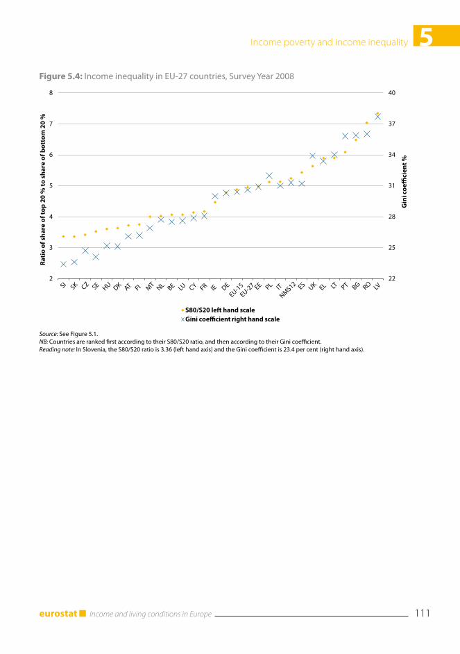
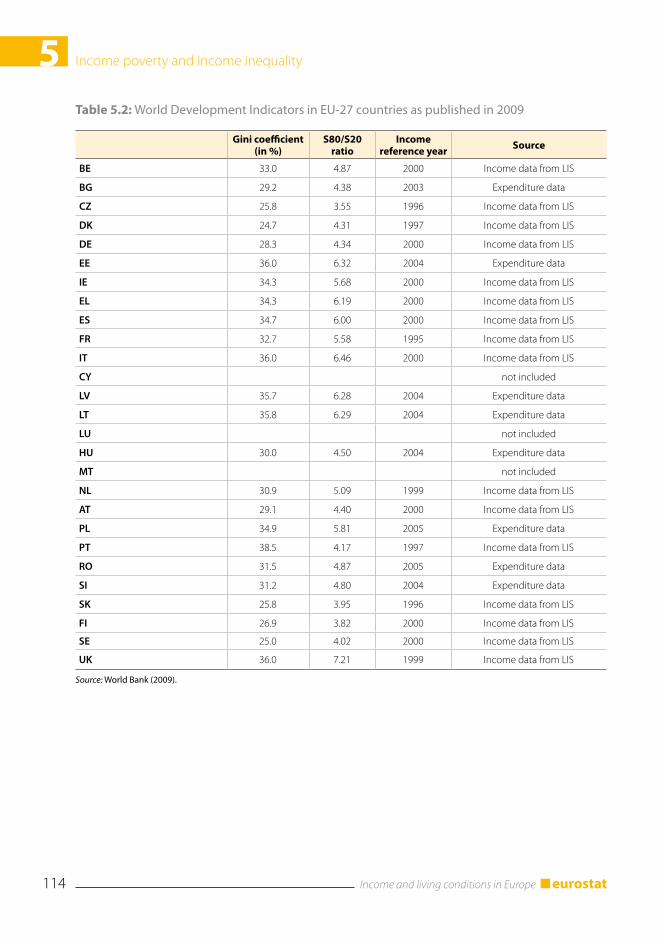
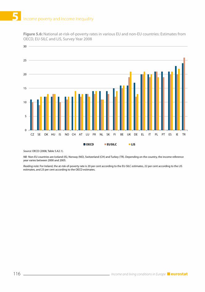
5.2.1 Evidence from EU-SILC on the risk of poverty ..........................................................1045.2.2 Evidence from EU-SILC on income inequality ...........................................................1095.2.3 Comparison with other cross-country sources ...........................................................112
5.3 Changes in income poverty and inequality over time ..............................................................1185.3.1 Monitoring trends in EU-SILC .....................................................................................1185.3.2 Changes in poverty risk ..................................................................................................1205.3.3 Changes in income inequality .......................................................................................1205.3.4 Comparison with national sources: a case study ........................................................120
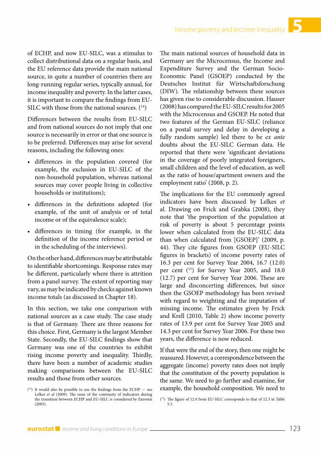
5.4 Monitoring progress ......................................................................................................................1245.4.1 An at-risk-of-poverty target...........................................................................................1245.4.2 Three indicators ..............................................................................................................126
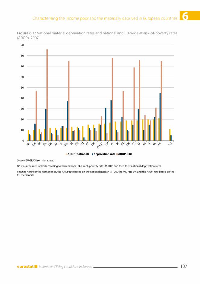
Characterising the income poor6. and the materially deprived in European countries (Alessio Fusco, Anne-Catherine Guio and Eric Marlier) ...............................................................1336.1 Introduction ...................................................................................................................................1346.2 Concepts and data .........................................................................................................................1346.3 Material deprivation and income poverty in the EU ................................................................1386.4 Relationship between income poverty and material deprivation ...........................................139
6.4.1 Factors affecting the relationship between income poverty and material deprivation ................................................................................................139
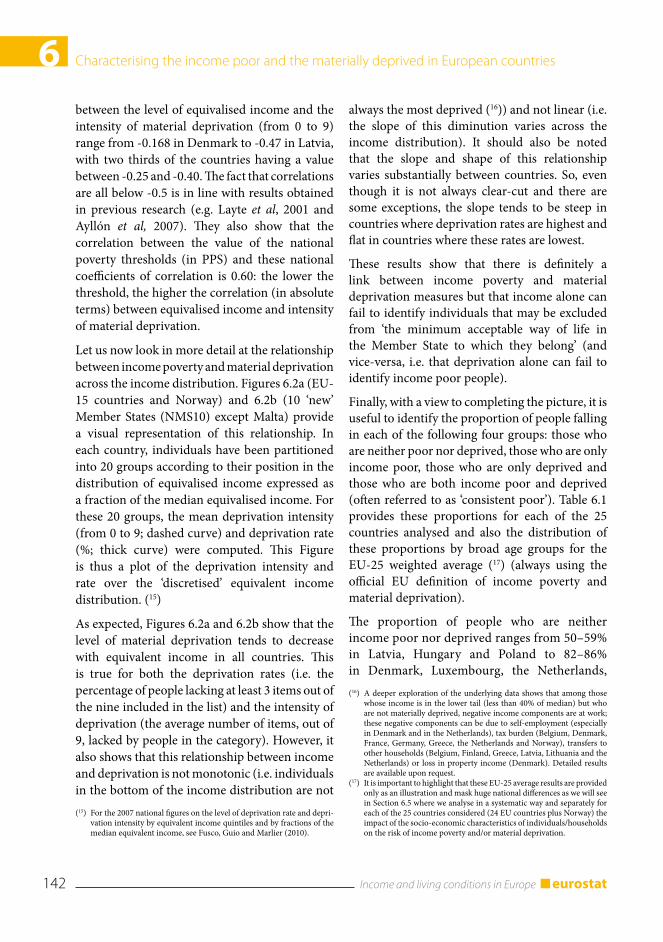
6.4.2 Results from EU-SILC ...................................................................................................1396.5 Characterisation of material deprivation and income poverty in the EU..............................144
6.5.1 Work intensity of the household ...................................................................................1466.5.2 Most frequent activity status ..........................................................................................1476.5.3 Household composition .................................................................................................1476.5.4 Age, gender and education .............................................................................................1486.5.5 Health problems ..............................................................................................................1486.5.6 Housing tenure status .....................................................................................................148
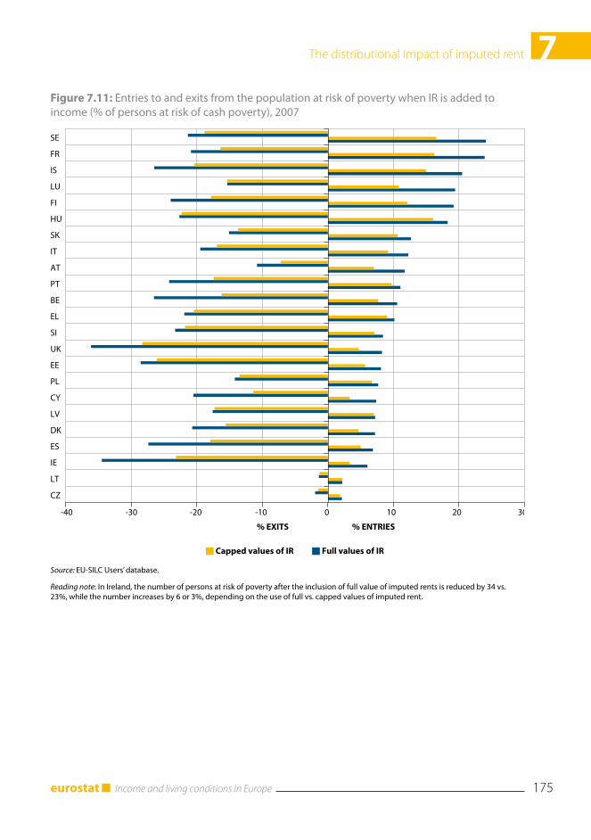
The distributional impact of imputed rent 7. (Hannele Sauli and Veli-Matti Törmälehto) .....................................................................................1557.1 Introduction ..................................................................................................................................1567.2 Theoretical and operational considerations ..............................................................................156
7.2.1 Housing wealth, housing consumption and disposable income ...............................1567.2.2 Measurement of imputed rentsas income ....................................................................1577.2.3 The data and the potential beneficiaries .......................................................................158
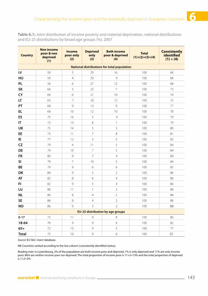
7.3 Imputed rents and income inequality .........................................................................................1597.3.1 Overall distributional effect ...........................................................................................159
7.4 Imputed rents and income poverty .............................................................................................1637.4.1 Imputed rents of outright owners .................................................................................1657.4.2 Imputed rents of tenants ................................................................................................165
7.5 Imputed rent and deprivation indicators ...................................................................................166
Income and living conditions in Europe eurostat10
7.5.1 The impact on non-monetary deprivation indicators ................................................1667.5.2 House rich — cash poor .................................................................................................168
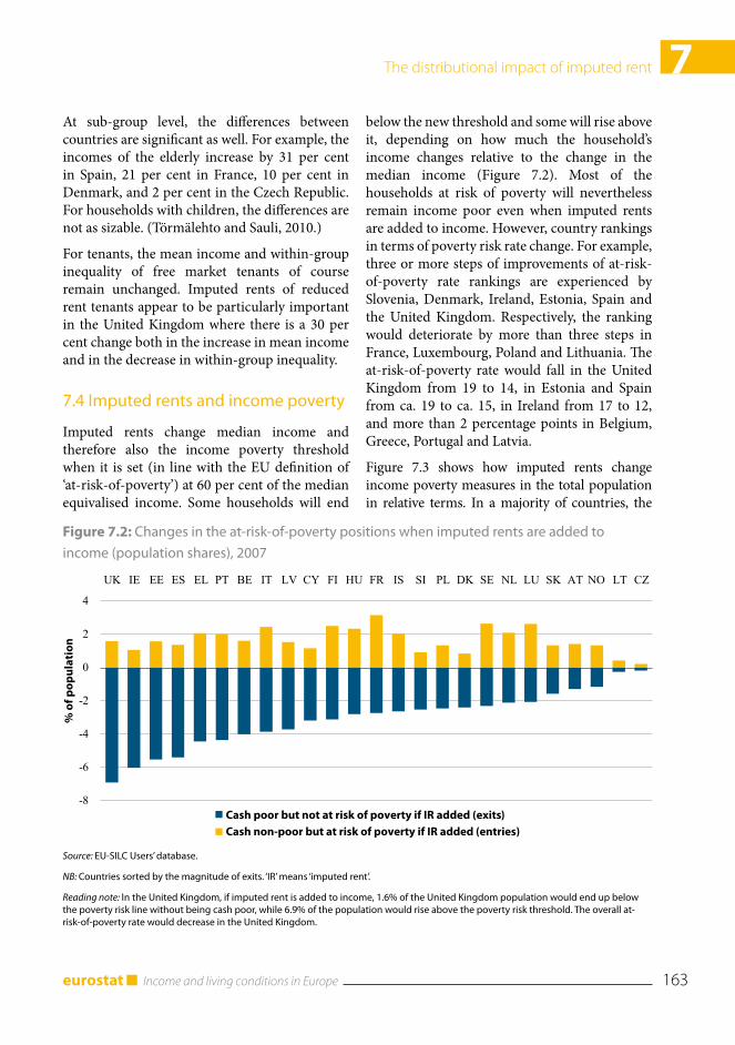
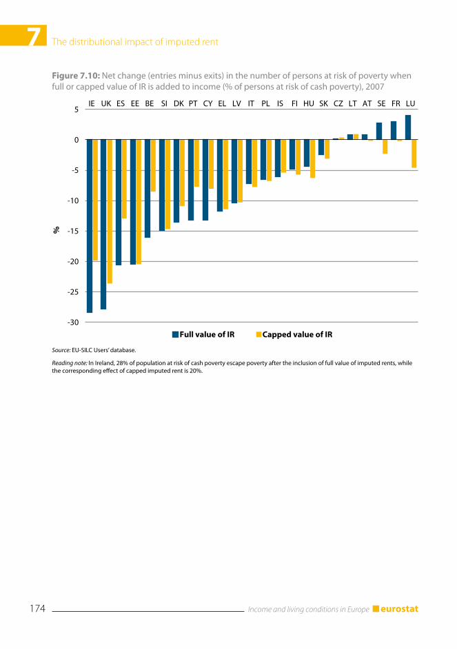
7.6 Imputed rents and alternative measures of the economic benefits of housing .....................1707.7 Capping imputed rents? ................................................................................................................1717.8 Summary and conclusions ...........................................................................................................173References .............................................................................................................................................177
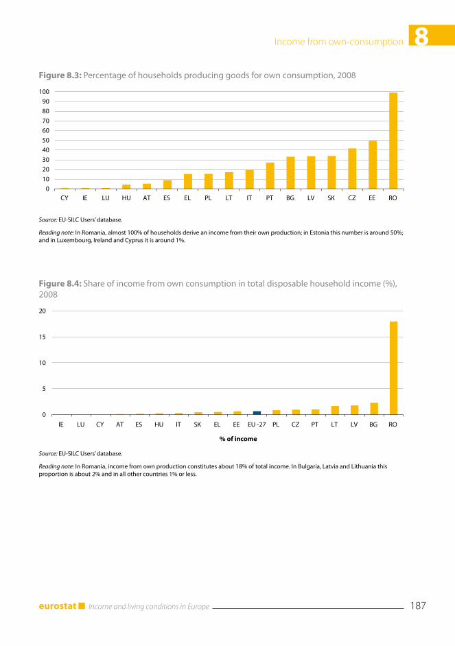
Income from own-consumption 8. (Merle Paats and Ene-Margit Tiit) ...........................................1798.1 Introduction ...................................................................................................................................180
8.1.1 Common recommendations for collecting the income data from own-consumption ..................................................................................................180
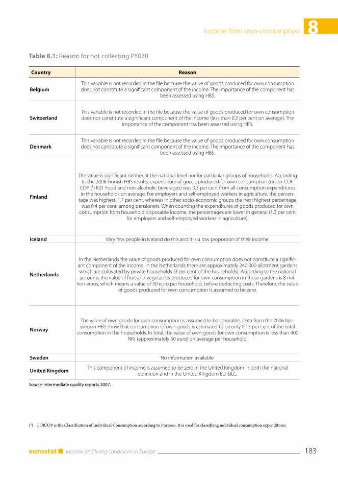
8.1.2 Recommendations in EU-SILC .....................................................................................1818.2 Collecting income from own-consumption in EU-SILC ........................................................182
8.2.1 Countries where income from own-consumption is not included ..........................1828.2.2 Countries where the income from own-consumption is included ...........................182
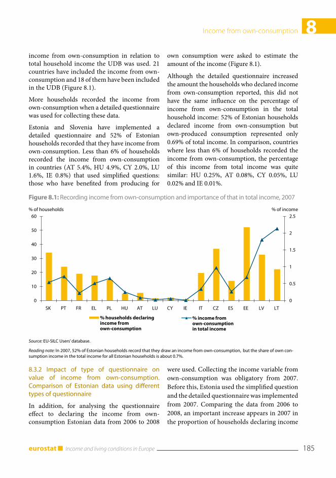
8.3 Results .............................................................................................................................................1848.3.1 Impact of type of questionnaire on value of income from own-consumption.
Comparison of EU countries using UDB data.............................................................1848.3.2 Impact of type of questionnaire on value of income from own-consumption.
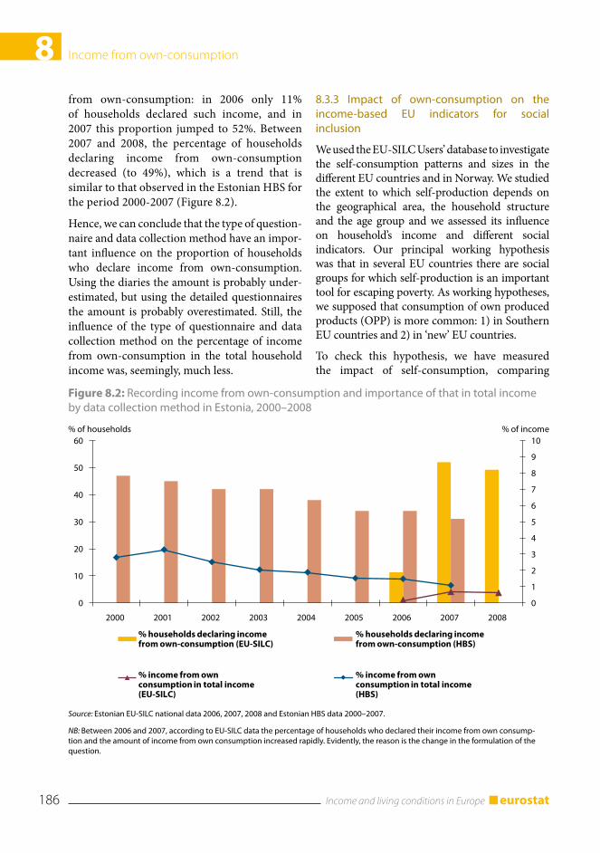
Comparison of Estonian data using different types of questionnaire .......................1858.3.3 Impact of own-consumption on the income-based EU indicators
for social inclusion ...........................................................................................................1868.3.4 Influence of own-consumption on poverty indicators ...............................................1898.3.5 Changes in poverty risk rates due to OPP in different household types..................191
8.4 Summary and conclusions ..........................................................................................................1928.4.1 Data comparability ..........................................................................................................1928.4.2 The impact of OPP on poverty reduction ....................................................................1938.4.3 Analysis of working hypotheses ....................................................................................1938.4.4 Recommendations ..........................................................................................................194
Socio-economic determinants of health in Europe 9. (Cristina Hernández-Quevedo, Cristina Masseria and Elias Mossialos) .....................................1959.1 Introduction ...................................................................................................................................1969.2 Literature review ............................................................................................................................1969.3 EU-SILC sample and variables ....................................................................................................199
9.3.1 Health variables ...............................................................................................................1999.3.2 Explanatory variables ......................................................................................................200
9.4 Methods ..........................................................................................................................................2009.4.1 Measuring inequality in health outcomes ....................................................................2009.4.2 Long-term inequalities in health ...................................................................................2019.4.3 Decomposition analysis..................................................................................................203
9.5 Results .............................................................................................................................................2039.5.1 Descriptive analysis .........................................................................................................2039.5.2 Evidence on socio-economic inequalities in health outcomes .................................2039.5.3 Sources of inequalities ....................................................................................................208
Social participation and social isolation 10. (Orsolya Lelkes) .............................................................21710.1 Introduction .................................................................................................................................21810.2 Data ...............................................................................................................................................21910.3 Social participation .....................................................................................................................220
10.3.1 Friendly Europe: frequency of social contacts ..........................................................22010.3.2 Social participation in voluntary activities ................................................................22310.3.3 Robustness of the results: comparison with the European Social Survey .............22510.3.4 Social participation makes people happy ...................................................................229
10.4 Social isolation .............................................................................................................................22910.4.1 An overview ...................................................................................................................23110.4.2 Social isolation by age: it tends to increase by age, although
relatively good informal support of help ......................................................................23510.4.3 Social isolation is greater among the poor and the unemployed, although
causality is unclear ...........................................................................................................23510.5 Conclusions ..................................................................................................................................236References .............................................................................................................................................239
Progress of living conditions — a dynamic model 11. of material deprivation for a European society (Matthias Till and Franz Eiffe) .........................24111.1 Introduction .................................................................................................................................24211.2 Understanding social inclusion as a multidimensional process............................................24211.3 The EU-SILC longitudinal component as a source for monitoring change .......................24411.4 Pan-European progress of living conditions ............................................................................24511.5 Evidence on gross and net change of material deprivation items .........................................24811.6 Winners and losers in a model of multiple changes ...............................................................252
11.6.1 Predicting net multiple improvement in Europe ......................................................25311.6.2 Predicting gross multiple change of material deprivation in Europe .....................259
11.7 Conclusions and recommendations .........................................................................................260References .............................................................................................................................................261
The distribution of employees’ labour earnings in the European Union: 12. data, concepts and first results (Andrea Brandolini, Alfonso Rosolia and Roberto Torrini) ...........................................................................................................................26512.1 Introduction .................................................................................................................................26612.2 Earnings in EU-SILC ..................................................................................................................26712.3 How does EU-SILC compare to other sources? ......................................................................26912.4 Time units and conversion rates ................................................................................................27312.5 Earnings distributions in EU countries ....................................................................................27612.6 The EU-wide distribution of gross earnings ............................................................................28212.7 Conclusions ..................................................................................................................................284References .............................................................................................................................................285
Educational intensity of 13. employment in Europe and the US (Donald R. Williams) ..........................................................................................................................28913.1 Introduction .................................................................................................................................29013.2 The research context....................................................................................................................29013.3 Methodology and data ...............................................................................................................291
13.3.1 Methodology ..................................................................................................................29113.3.2 Data .................................................................................................................................294
Income and living conditions in Europe eurostat12
13.4 Employment shares by skill level ...............................................................................................29413.5 Demographic differences ............................................................................................................29913.6 Summary and conclusions .........................................................................................................301References .............................................................................................................................................304
Assessing and analysing in-work poverty risk 14. (Sophie Ponthieux) ..............................................30714.1 Introduction .................................................................................................................................30814.2 Definitions of workers and subsequent analysis
of a working poor-type phenomenon ......................................................................................30814.2.1 Three definitions of workers: active, employed, in-work .........................................30914.2.2 Impact on the ‘size of the problem’ .............................................................................30914.2.3 Impact on the analysis of the problem .......................................................................310
14.3 Poverty risk at the individual level or working households: two other ways to look at work and poverty risk ....................................................................317
14.3.1 At the individual level: a complementary approach in terms of ‘poverty in earned income’ .............................................................................................317
14.3.2 At the household level: in-work households? ............................................................32214.4 Conclusions ..................................................................................................................................324References .............................................................................................................................................327
The impact of basic public services on the distribution 15. of income in European countries (Rolf Aaberge, Audun Langørgen and Petter Lindgren) ................................................................32915.1 Introduction .................................................................................................................................33015.2 Definition and measurement of extended income ..................................................................331
15.2.1 Cash income ..................................................................................................................33115.2.2 The value of public services .........................................................................................33215.2.3 Allocation of public services ........................................................................................33215.2.4 Accounting for needs ....................................................................................................334
15.3 Cross-country comparison of income inequality and poverty..............................................33715.3.1 Main results ...................................................................................................................33915.3.2. Interaction between incomes and needs for public services ..................................339
Distributional effects of direct taxes and social transfers (cash benefits) 16. (Vaska Atta-Darkua and Andrew Barnard) .....................................................................................34516.1 Introduction .................................................................................................................................34616.2 Source, methodology and concepts ..........................................................................................346
16.2.1 Source .............................................................................................................................34616.2.2 Methodology ..................................................................................................................34616.2.3 Issues of income inequality ..........................................................................................348
16.3 Results ...........................................................................................................................................34916.3.1 Overall effect ..................................................................................................................34916.3.2 Results for retired households .....................................................................................35716.3.3 Comparison of Gini coefficients .................................................................................360
Policy simulation across countries using EUROMOD: stress testing European welfare 17. systems for unemployment (Francesco Figari, Andrea Salvatori and Holly Sutherland) ..........36917.1 Introduction .................................................................................................................................37017.2 EUROMOD ................................................................................................................................370
17.2.1 Data .................................................................................................................................37117.3 Methodological approach ...........................................................................................................372
17.3.1 Counterfactual scenarios .............................................................................................37217.3.2 Sample of interest ..........................................................................................................37317.3.3 Indicators........................................................................................................................373
17.4 Welfare systems for the unemployed in 2008 ..........................................................................37417.5 Relative resilience .......................................................................................................................37617.6 Protection against risk of poverty .............................................................................................37817.7 Cost of protection ........................................................................................................................38117.8 Conclusions ..................................................................................................................................382References .............................................................................................................................................385
Beyond 18. GDP, measuring well-being and EU-SILC (Anthony B. Atkinson, Eric Marlier and Pascal Wolff) ................................................................. 38718.1 Introduction .................................................................................................................................38818.2 Conceptual issues ........................................................................................................................388
18.2.1 Drivers vs. outcomes .....................................................................................................38918.2.2 Change in population vs. change in individual well-being .....................................38918.2.3 Frequency and timeliness .............................................................................................38918.2.4 Different needs for different sub-populations ...........................................................39018.2.5 Household vs. individual well-being ..........................................................................39018.2.6 Flow vs. stock .................................................................................................................390
18.3 Composite indices .......................................................................................................................39018.4 EU-SILC and other household data sources ............................................................................39118.5 Coherence among household surveys ......................................................................................39318.6 Coherence of income data at an aggregate level ......................................................................394
18.6.1 Household income ........................................................................................................39418.6.2 Imputed rent on owner-occupied housing ................................................................39418.6.3 Individual consumption expenditure of general government ................................39618.6.4 Pensions ..........................................................................................................................39618.6.5 Sampling and non-sampling errors ............................................................................39618.6.6 Reconciliation ................................................................................................................396
Appendices ..........................................................................................................................................399Appendix 1: List of Net-SILC members ............................................................................................400Appendix 2: Country official abbreviations and geographical aggregates ...................................401
Country official abbreviations ...............................................................................................401Geographical aggregates ..........................................................................................................401
Appendix 3: Other abbreviations and acronyms .............................................................................402Appendix 4: Author index ..................................................................................................................404Appendix 5: Subject index ..................................................................................................................410
Income and living conditions in Europeeurostat 15
List of tables, figures and boxes
TablesTable 2.1: Minimum effective sample size for the cross-sectional and longitudinal components by country ........................................................................................................ 45Table 2.2: Basic concepts and definitions (Are the national definitions comparable with those of the standard EU-SILC?), 2008 ................................................................................................... 51Table 3.1: Households receiving income from self-employment, 2007 ........................................................ 63Table 3.2: Ratio of upper percentiles to the median, 2007 Total disposable household income (HY020).................................................................................................. 65Table 3.3: Unit non-response (cross-sectional sample, 2007) ....................................................................... 67Table 3.4: Item non-response: income from self-employment (PY050), 2007 ............................................ 70Table 3.5: Estimates of standard errors and components of design effects, 2005–2006 ............................. 74Table 4.1: Distribution of household types, 2007 ............................................................................................ 84Table 4.2: Distribution of households by number of children, 2007 ........................................................... 86Table 4.3: Household type in which children live, 2007 ................................................................................. 87Table 4.4: Young people: transitions and percentages living alone, 2007 ..................................................... 90Table 4.5: Percentage of partnerships which are cohabiting rather than marital partnerships fordifferent age groups of women, 2007 .................................................................................... 91Table 4.6: The living arrangements of people aged 65 years and over, percentages, 2007 ......................... 93Table 4.7: Factor loadings, 2007 ......................................................................................................................... 95Table 5.1: National at-risk-of-poverty thresholds for a household consisting of 2 adults and 2 children below 14 in EU-27 countries (PPS), Survey Year 2008........................................105Table 5.2: World Development Indicators in EU-27 countries as published in 2009...............................114Table 5.3: National at-risk-of-poverty rates in EU-27, Survey Years 2003–2008 ......................................119Table 5.4a: Income inequality in EU-27 countries: S80/S20 ratio, Survey Years 2003-2008 ...................121Table 5.4b: Income inequality in EU-27 countries: Gini coefficients, Survey Years 2003-2008 ....................................................................................................................................122Table 6.1: Joint distribution of income poverty and material deprivation, national distributions and EU-25 distributions by broad age groups (%), 2007 ......................................143Table A.6.1 (1/2): Determinants of income poverty and material deprivation, 2007 ..............................152Table A.6.1 (2/2): Determinants of income poverty and material deprivation, 2007 ..............................153Table 7.1: Imputed rent as income: the estimation methods in EU-SILC, 2007 ......................................158Table 7.2: Changes in income inequality when moving from cash incomes to incomes augmented with imputed rents, 2007..........................................................................160Table 7.3: EU-wide income inequality indicators (Germany excluded), 2007 ..........................................162Table 7.4: At risk of cash poverty rates, at risk of poverty rates after inclusion of imputed rents and at risk of poverty rates after inclusion of capped imputed rents (% of persons), 2007 .....................172Table 8.1: Reason for not collecting PY070 ....................................................................................................183Table 8.2: Differences between the poverty risk rates without and with OPP for different types of household (households, percentage points), 2008 ...................................................192Table 9.1: Long-term concentration indices and mobility indices, 2005-2007 .........................................207
Income and living conditions in Europe eurostat16
Table 10.1: Participation in various types of informal activities during the last year, % of population per country, 2006 ..............................................................................224Table 10.2: Ability to get help and frequency of getting together with relatives or friends (%), 2006 ...225Table 10.3: Share of population meeting relatives of friends at least once a week (%). Comparison of EU-SILC 2006 data with those of the European Social Survey (ESS) 2004 and 2006 ..226Table 10.4: Share of population helping others (outside own household) and those engaged in political actions during the last year, %. Comparison of EU-SILC 2006 data with those of the European Social Survey (ESS) 2004 and 2006 ........................................................................................228Table 10.5: Correlation between measures of subjective well-being and social participation, 2006 ......229Table 10.6: Alternative measures of social isolation across EU countries, share of population affected (%), 2006 ...........................................................................................................233Table 11.1: Comparison of the longitudinal pattern of the material deprivation indicator and number of changed items (in % of the longitudinal population), 2006-2007 ...................252Table 11.2: OLS Regression model for predicted net and gross multiple changes ....................................254Table 12.1: Earnings in EU-SILC and in national accounts in 2006 (millions of euros and per cent) ......................................................................................................................270Table.12.2: Statistics for the distribution of gross earnings in EU countries, 2006...................................278Table 12.3: Statistics for the EU-wide distribution of gross earnings, 2006 ..............................................281Table 12.4: Variance decomposition of the logarithm of monthly full-time equivalent earnings (absolute values and percentage shares in italics), 2006 ...........................................284Table A.12.1: Alternative definitions of employee cash or near cash income in EU-SILC (%). Survey Year 2007 ...................................................................................................287Table 13.1: Occupational classifications, by skill level, 2007........................................................................293Table 13.2: Occupational distributions by gender, age and citizenship, selected EU-SILC countries combined (per cent in occupation), 2007 .....................................................300Table 13.3: Skill Distributions by gender, age and citizenship, selected EU-SILC countries combined (per cent in skill category), 2007 .................................................301Table A.13.1: Sample sizes ................................................................................................................................305Table 14.1: Active, employed, in-work (%), 2007 ..........................................................................................311Table 14.2: Poverty risk and workers at risk of poverty by employment status (%), 2007 .......................312Table 14.3: Poverty risk within full year employment and activity profile of workers at risk of poverty (%), 2007 ...........................................................................................................313Table 14.4: Workers at risk of poverty and concentration of poverty risk by household type (%), 2007 .................................................................................................316Table 14.5: Poverty in earned income and poverty risk of ‘in-work’ workers, 2007 ................................320Table 14.6: Poverty in earned income and poverty risk by gender, 2007 ...................................................321Table 15.1: Alternative definitions of equivalent income .............................................................................337Table 15.2: Equivalence scales by household type, 2006 ..............................................................................338Table 15.3: Gini-coefficient for the distribution of income by income definition and country, 2006 .........................................................................................................340Table 15.4: At-risk-of-poverty by income definition and country (%), 2006 ............................................340Table 15.5: At-risk-of-poverty decomposed by subsets according to income definition and country (%), 2006 ..................................................................................................341
Income and living conditions in Europeeurostat 17
Table 15.6: At-risk-of-poverty for cash income measure (EU scale), by country and by quintiles of the needs index (%), 2006 ...........................................................................341Table 15.7: At-risk-of-poverty for extended income measure (EU scale), by country and by quintiles of the needs index (%), 2006 ...........................................................................342Table 15.8: At-risk-of-poverty for extended income measure (NA scale), by country and by quintiles of the needs index (%), 2006 ...........................................................................342Table 16.1a: Income quintile share ratios (S80/S20) for ALL households, 2007 .......................................351Table 16.1b: Gini and concentration coefficients for ALL households (%), 2007 .....................................352Table 16.2: Summary of the size of cash benefits and direct taxes as a percentage of gross income for ALL households, 2007) .......................................................................353Table 16.3: Cash benefits as the percentage of gross income by quintile groups for ALL households, 2007 ................................................................................................356Table 16.4: Direct taxes as the percentage of gross income by quintile groups, 2007 ..............................358Table 16.5: Gini and concentration coefficients for RETIRED households, 2007 ....................................361Table 16.6: Summary of the size of cash benefits and direct taxes as a percentage of gross income for RETIRED households, 2007 ..........................................................................................362Table 16.7: Cash benefits as the percentage of gross income by quintile groups for RETIRED households, 2007 ......................................................................................363Table 16.8: Direct taxes as the percentage of gross income by quintile groups for RETIRED households, 2007 ......................................................................................365Table 16.9: Comparing Gini coefficients for disposable income by country, 2007 ...................................366Table 16.10: Gini coefficients for income — the United Kingdom .............................................................367Table 17.1: Characteristics of the new unemployed ......................................................................................374Table 17.2: Average Relative Welfare Resilience Indicator (RWRI) with and without unemployment benefits (UBs) ..........................................................................................376Table 17.3: Proportion of the new unemployed protected from falling below the poverty threshold in unemployment, with and without unemployment benefits (UBs) .......................................382
figures
Figure 2.1: EU-SILC implementation ............................................................................................................... 39Figure 2.2: Fieldwork period, 2008 ................................................................................................................... 48Figure 2.3: Average interview duration per individual, 2008 ........................................................................ 49Figure 2.4: Overall personal non-response rates, 2008 .................................................................................. 50Figure 3.1: Types of errors in surveys ............................................................................................................... 60Figure 3.2: Components of non-response ........................................................................................................ 66Figure 4.1: Example of a household grid ......................................................................................................... 82Figure 4.2: Clusters arising from Principal Components Analysis, 2007 .................................................... 96Figure 5.1: National at-risk-of-poverty rates in EU-27, Survey Year 2008 ................................................107Figure 5.2: National at-risk-of-poverty rates for children and for overall population in EU-27, Survey Year 2008 ......................................................................................108Figure 5.3: National at-risk-of-poverty rates and relative median at-risk-of-poverty gap in EU-27, Survey Year 2008 ......................................................................................110Figure 5.4: Income inequality in EU-27 countries, Survey Year 2008 ........................................................111
Income and living conditions in Europe eurostat18
Figure 5.5: National at-risk-of-poverty rates and S80/S20 ratios, EU-27, Survey Year 2008 ..................113Figure 5.6: National at-risk-of-poverty rates in various EU and non-EU countries: Estimates from OECD, EU-SILC and LIS, Survey Year 2008 .............................116Figure 5.7: National Gini coefficients in various EU and non-EU countries: Estimates from OECD, EU-SILC and LIS, Survey Year 2008 ......................................................................117Figure 5.8: Millions taken out of income poverty and number of EU countries that need to be involved, Survey Year 2008 ...........................................................................125Figure 5.9: Multiple indicators for the Europe 2020 target, figures for EU-27 in million of persons, Survey Year 2008 .............................................................................................127Figure 5.10: Extent of overlap according to the three indicators on which the Europe 2020 target on social inclusion is based, EU-27, Survey Year 2008 ..............................................128Figure 6.1: National material deprivation rates and national and EU-wide at-risk-of-poverty rates (AROP), 2007 ..........................................................................................137Figure 6.2a: Intensity of deprivation (from 0 to 9) and deprivation rate (%) according to the level of equivalised income (% median), EU-15 and Norway, 2007 .............................140Figure 6.2b: Intensity of deprivation (from 0 to 9) and deprivation rate (%) according to the level of equivalised income (% median), NMS10 excluding Malta, 2007 ....................141Figure 7.1: Changes in income inequality and average income (without imputed rent --> with imputed rent) , 2007 ..................................................................................161Figure 7.2: Changes in the at-risk-of-poverty positions when imputed rents are added to income (population shares), 2007 ...................................................................163Figure 7.3: Relative changes in the FGT income poverty measures: total population (%), 2007 ...........164Figure 7.4: Contributions of owner households (bars) to the change in total poverty risk rates (line), 2007 .............................................................................................................164Figure 7.5: Contributions of tenant households (bars) to the change in total poverty risk rates (line), 2007 ...................................................................................167Figure 7.6: Material deprivation rates in populations exiting from, entering in and remaining in population at risk of poverty due to inclusion of imputed rents in income, 2007...................................................................................................167Figure 7.7: Changes in material deprivation and overcrowding in the population at risk of poverty due to the inclusion of imputed rents in income, 2007 ....................................................................................................................169Figure 7.8: Share of cash poor house rich persons with imputed rent values that at least double their cash disposable income, 2007 ...........................................................169Figure 7.9: Change of the range of the income share of imputed rents by capping based on overcrowding criteria, persons with non-zero IR, 2007 ..........................................172Figure 7.10: Net change (entries minus exits) in the number of persons at risk of poverty when full or capped value of IR is added to income (% of persons at risk of cash poverty), 2007 ....................................................................174Figure 7.11: Entries to and exits from the population at risk of poverty when IR is added to income (% of persons at risk of cash poverty), 2007 ......................175Figure 8.1: Recording income from own-consumption and importance of that in total income, 2007 ............................................................................................................................185Figure 8.2: Recording income from own-consumption and importance of that in total income by data collection method in Estonia, 2000–2008 ......................................................................................................186
Income and living conditions in Europeeurostat 19
Figure 8.3: Percentage of households producing goods for own consumption, 2008 ..............................187Figure 8.4: Share of income from own consumption in total disposable household income (%), 2008 ...........................................................................................187Figure 8.5: At-risk-of-poverty rate without and with OPP, % of people, 2008 ..........................................188Figure 8.6: Relative median poverty risk gap (%), 2008 ...............................................................................188Figure 8.7: In-work poverty risk without and with OPP, % of people, 2008 ............................................190Figure 8.8: Income inequality (S80/S20 ratio) with and without OPP, 2008 .............................................190Figure 9.1: Concentration curve for an indicator of health limitations compared to the 45-degree line (diagonal) of perfect equality – The example of Cyprus in 2007 ................................202Figure 9.2: Percentage of individuals reporting very good or good self-assessed health, 2005-2007 ......................................................................................................................204Figure 9.3: Percentage of individuals reporting health limitations in their daily activity, 2005-2007 .....................................................................................................................204Figure 9.4: Percentage of individuals reporting a long-standing chronic illness, 2005-2007 ..................205Figure 9.5: Concentration indices for health limitations for waves 2005, 2006 and 2007 .......................206Figure 9.6: Decomposition results for the 2007 health model ....................................................................209Figure 10.1: Frequency of getting together with relatives (%), 2006 ..........................................................221Figure 10.2: Percentage of population who have frequent personal contact with relatives and friends, 2006 ........................................................................................................221Figure 10.3: ‘Cyber’ contacts versus personal meetings: ratio of those with cyber contact compared to those with personal meetings minimum once a week, 2006 ..........................................................................................222Figure 10.4: Social isolation across EU countries: not able to ask any relative, friend or neighbour for help (%), 2006 .........................................................230Figure 10.5: Social isolation at an EU level: share of population never meeting friends, relatives or either of these (%), 2006 ....................................232Figure 10.6: Ratio of those with no friends by age groups compared to the total population, 2006 .........................................................................................................234Figure 10.7: Ratio of those with no help by age groups compared to the total population, 2006 ............................................................................................................................236Figure 10.8: Ratio of those with ‘no friends’ by poverty status (ratio between those at risk of poverty and those not at risk), 2006...........................................................237Figure 10.9: Ratio of those with ‘no help’ by employment status (Ratio between particular groups and the total working age population), 2006 ......................................238Figure 11.1: Analytic framework for social exclusion in Europe ................................................................243Figure 11.2: Importance of non-market services in the disposable incomes of private households*), national accounts, 2008............................................246Figure 11.3: Gross change for deprivation items (%), 2006-2007 ...............................................................249Figure 11.4: Net change for deprivation items (%), 2006-2007 ...................................................................249Figure 11.5: Gross change in deprivation items for working age individuals who increase or decrease labour market participation (%), 2006-2007 ................................250Figure 11.6: Map of predicted net multiple changes in the reference group (%), 2006-2007 ................256Figure 11.7: Map of predicted gross multiple changes in the reference group (%), 2006-2007 ..............258
Figure 12.1: Map of available net and gross employee cash or near cash income in EU-SILC, Survey Year 2007 ..................................................................................................269Figure 12.2: Tax wedge on labour costs for low wage earners in 15 EU countries (%), Survey Year 2007 ..........................................................................................................272Figure 12.3: Impact on measured real wages of the choice of the PPP index, 2006 .................................274Figure 12.4: Distribution of real monthly full-time equivalent gross earnings in EU countries (thousands of euros in PPS-HFCE), 2006 ......................................................................................................275Figure 12.5: Decile ratio of gross earnings in EU countries, 2006 ..............................................................277Figure 12.6: Distribution of real monthly full-time equivalent earnings in selected EU countries by different definitions of earnings (PPS-HFCE), 2006 ...............................................................................280Figure 13.1: Employment shares by skill level, EU and US, 2007 ...............................................................295Figure 13.2: Employment shares by skill level, selected EU-SILC countries, 2007 ..................................297Figure 13.3: Cumulative employment shares by skill level and demographic group, selected EU-SILC countries, 2007 ...................................................................................................................302Figure 14.1: Employment problems (*) and poverty risk (ratio of % of women to % of men) ..............318Figure 14.2: Poor in earned income/not poor in earned income (%), 2007 ..............................................321Figure 14.3: Poverty in earned income in in-work poverty risk by gender (%), 2007 .............................322Figure 16.1: Concentration curve for benefits (5 households) ....................................................................349Figure 16.2: Summary of the effect of taxes and benefits on reducing income inequality of the Gini coefficient (percentage point reduction in Gini coefficient), 2007 .........................................355Figure 16.3: Scatter plot of disproportionality of benefits (%) vs. their average rate (%), 2007 ..............359Figure 16.4: Scatter plot of disproportionality of taxes (%) vs. their average rate (%), 2007 ...................359Figure 17.1: Average Relative Welfare Resilience Indicator (RWRI) and post-unemployment household income composition, with unemployment benefits ...........................................................................................................................377Figure 17.2: Average Relative Welfare Resilience Indicator (RWRI) and post-unemployment household income composition by household income quintile group, with unemployment benefits.................................................................................................379Figure 17.3: The proportion of new unemployed at risk of falling below the poverty threshold, with unemployment benefits ........................................................................380Figure 17.4: Average budgetary cost per unemployed person (as a proportion of per-capita national disposable income) .......................................................................383Figure 18.1: Linking national income flows to household disposable income .........................................395
Boxes
Box 14.1: Definitions of workers .....................................................................................................................310Box 14.2: Activity profiles .................................................................................................................................314Box 14.3: An indicator of poverty in earned income ....................................................................................319
1Living conditions in Europe and the Europe 2020 agendaAnthony B. Atkinson and Eric Marlier (1)
(1) Anthony B. Atkinson is at Nuffield College, Oxford, and the London School of Economics (UK); Eric Marlier is with the CEPS/INSTEAD Research Institute (Luxembourg). The authors would like to thank the European Commission for their support of the Network. The European Commission bears no responsibility for the analyses and conclusions, which are solely those of the authors. Addresses for correspondence: [email protected] and [email protected].
Income and living conditions in Europe eurostat22
1 Living conditions in Europe and the Europe 2020 agenda
1.1 Introduction
This book is about the incomes and living standards of the people of Europe. The
reader will learn about employment, income inequality and poverty, housing, health, education, deprivation and social exclusion. The chapters tell about how the workers of Europe earn their living, about the living arrangements of Europeans, about their social participation, and about the ways in which their incomes are affected by taxes and transfers. The book addresses many of the social issues confronting Europe. How much income poverty is there in Europe? Is inequality increasing? Does a job guarantee escape from income poverty? How is Europe’s welfare state coping with the economic crisis?
Evidence about these important dimensions of European society comes from a data source that has been progressively implemented since 2003: the EU Statistics on Income and Living Conditions (EU-SILC). EU-SILC represents a powerful instrument for the analysis of the economic and social state of the European Union (EU) as well as a growing number of non-EU European countries. It is a large investment, and requires substantial effort on the part of the European Statistical System (ESS), but it is already playing a major role in the provision of key socio-economic statistics. EU-SILC has boosted the possibilities of carrying out comparative analyses of income distribution and living conditions in Europe. It is therefore important to take stock of what has been achieved and to consider possible future applications and developments of EU-SILC. It was for this reason that the Net-SILC Network was established, in response to a call for applications by the Statistical Office of the European Union (Eurostat) in 2008. The Network, coordinated by Eric Marlier in close cooperation with Anthony B. Atkinson, consisted of eight teams from participating ESS bodies (seven National Statistical Institutes (Austria, the Czech Republic, Estonia, Finland, Italy,
Norway, the United Kingdom) and the CEPS/INSTEAD research institute in Luxembourg), eight teams from academic institutions (2), with the additional participation of the Bank of Italy and the French National Statistical Institute (INSEE). Net-SILC was thus an ambitious 18-partner Network bringing together expertise from both data producers (directly involved in the collection of EU-SILC data) and data users.
The present book represents a major output from the Net-SILC Network, but not all of the scientific work produced in the context of Net-SILC could be covered. In the book, we have focused on the research findings that we believe are likely to be of interest to the general reader and to those concerned with policy. We asked the authors of individual chapters to make them as accessible as possible to the non-specialist. More technical material, and the output from the more methodological work packages, are available in the series Eurostat methodologies and working papers.
Our emphasis in this book reflects the fact that EU-SILC plays a central role in the promotion of the Social Agenda of the EU. (3) In its list of the main users of EU-SILC data, Eurostat puts at the head ‘institutional users’ and in particular the EU Social Protection Committee (SPC), the body that has been in charge of coordinating and monitoring together with the European Commission the Open Method of Coordination on social protection and social inclusion (Social OMC) since it was launched back in 2000. (4) (2) Nuffield College (UK), Wissenschaftszentrum Berlin für Sozialforsc-
hung (‘WZB-Berlin’, Germany), Institut Wallon de l’Evaluation, de la Prospective et de la Statistique (‘IWEPS’, Belgium), European Centre for Social Welfare Policy and Research (Austria), London School of Economics (UK), Institute for Social and Economic Research of the University of Essex (ISER, UK), University of Sienna (Italy), Kent State University (USA).
(3) On the ‘Renewed Social Agenda’ adopted by the European Commission on 2 July 2008, see: http://ec.europa.eu/social/main.jsp?catId=547.
(4) The SPC consists of officials from mainly Employment and Social Af-fairs Ministries in each Member State as well as representatives of the European Commission; it reports to the EU ‘Employment, Social Poli-cy, Health and Consumer Affairs’ (EPSCO) Council of Ministers. In the context of the Social OMC, all EU countries cooperate in the fields of social inclusion, pensions, and healthcare and long-term care. For more information on the SPC and the Social OMC, see European Commission website http://ec.europa.eu/social/main.jsp?catId=750&langId=en.
1Living conditions in Europe and the Europe 2020 agenda
During the life of the Network, EU-SILC took on particular significance with the adoption in June 2010 by the European Council of the Europe 2020 Headline Targets. (5) The fifth of these targets relates to poverty and social exclusion, and EU-SILC will be the reference source for the three indicators on which this new EU target is based (as discussed further below in Section 1.4 and in Chapter 5).
The EU at the time of writing has 27 Member States. Its current coverage reflects the Enlargements that have taken place in recent years. As a result of the May 2004 Enlargement, the EU grew from 15 to 25 Member States. The 10 new EU countries were Cyprus, the Czech Republic, Estonia, Hungary, Latvia, Lithuania, Malta, Poland, Slovenia and Slovakia. In January 2007 (the most recent Enlargement), Bulgaria and Romania joined. (6) Readers should note that in a number of chapters Bulgaria, Malta and Romania are not covered because data for these countries were not available from the EU-SILC Users’ database (UDB) to which the Network had access.
Increasingly, EU-SILC is being recognised as a significant international statistical resource, not least because its coverage is not confined to the 27 EU countries (EU-27). The ‘framework’ approach adopted when establishing EU-SILC is an innovative experiment that may have lessons for other areas of EU statistics. It is hoped therefore that the Net-SILC findings will appeal to readers from outside the EU. In particular, it is relevant to the world-wide interest in moving Beyond GDP, and this is the subject of Chapter 18. Our focus in the book is on EU-SILC, but reference should be made to other important EU sources of evidence about incomes and living conditions. These (5) The European Council, which brings together the EU Heads of State
and Government and the President of the European Commission, defines the general political direction and priorities of the EU. Every spring, it holds a meeting that is more particularly devoted to eco-nomic and social questions – the Spring European Council. With the entry into force of the Treaty of Lisbon on 1 December 2009, it has become an official institution and has a President. The Con-clusions of the June 2010 European Council are available from: http://ec.europa.eu/eu2020/pdf/council_conclusion_17_june_en.pdf.
(6) See list of ‘Country official abbreviations and geographical aggregates’ (Appendix 2).
EU sources include inter alia the Labour Force Surveys (used for example in Chapter 17), the Eurobarometer (used for example in Chapter 11), and the European Social Survey (used for example in Chapter 10). An important resource for the analysis of tax and benefits is the EUROMOD model, described in Chapter 17. A major reference point for a number of chapters is the data provided by the Luxembourg Income Study (LIS) and the analysis by the Organisation for Economic Cooperation and Development (OECD).
In the remainder of this Introduction, we describe (Section 1.2) the contents of the book and the other outputs from the Net-SILC Network, summarise (Section 1.3) the main lessons for the future development of EU-SILC, and consider (Section 1.4) the role that EU-SILC may play in the new political context of formation of national targets and related social policies within the broader framework of EU targets. We also get back to the latter in Chapter 5.
1.2 Outline of the contents
The book opens in Chapter 2 with a description of the EU-SILC data, provided by Eurostat. The description of statistical sources and methods may not strike the reader as the most gripping subject. Many universities have removed courses on statistical sources from their social science syllabi, replacing them by courses that are more eye-catching or more mathematical. But data are very important, and cannot be taken for granted. While data can today be downloaded from many sources and immediately turned into tables and graphs or used to estimate statistical models, they can only be reliably used on the basis of an appreciation of their strengths and weaknesses. Unless one knows something about the origins of the data, and the processing methods that have been applied, a data user – even the reader of tables and graphs in this book – can go seriously wrong. For the same reason, we urge readers to consult Chapter 3 by Verma and Betti on data accuracy in EU-SILC. The authors have summarised succinctly, and in a largely non-
1 Living conditions in Europe and the Europe 2020 agenda
technical manner, the different dimensions of data quality. As a minimum, the reader should look at Table 3.1, which lists the manifold possible sources of error.
The risk in the other direction is that, rather than ignoring the possible shortcomings of the data, the reader is overwhelmed by the catalogue of possible sources of error. How, the reader may ask, can any weight be attached to the outcome of such a process? Such a reaction goes too far. One of the aims of Chapters 2 and 3 is to describe the procedures applied to deal with the potential problems and the checks that are applied. Indeed, many of the chapters consider the validity of the EU-SILC data, including comparisons with other statistical sources. These checks reveal that there are issues that need to be addressed (see Section 1.3 below), and some of the results must be hedged by qualifications. The overall picture, however, is re-assuring, and, in our view, the EU-SILC data have survived well the demands placed on them in the research projects carried out as part of Net-SILC.
The substantive contents start with Chapter 4, where Iacovou and Skew examine the evidence about household structure in Europe. The differences across Europe in household formation are one of the features obvious to any traveller, and the data confirm a number of these impressions. In the Nordic countries, for example, around a quarter of all households consist of a single adult aged under 65, whereas in Cyprus, Portugal and Spain the proportion is less than a tenth. What is less obvious is how to draw out common patterns, particularly with the Enlargement from EU-15 to EU-25, and a particular focus of the chapter is the integration of ‘New’ Member States who joined the EU in May 2004 into the analysis. Their statistical analysis highlights three factors: the importance of the extended family, the stability of the intimate relationship, and the level of fertility. The role of the first two factors is conveniently summarised in Figure 4.2.
After asking who lives in the household, the next
question may well be ‘what is their income?’ Income is an important variable for Europe’s households. People are naturally concerned with how much they receive each month in the form of earnings from work (employment or self-employment), from pensions, from other government transfers such as unemployment benefits, family benefits or sick pay, and from their savings. In Chapter 5, Atkinson, Marlier, Montaigne and Reinstadler examine the distribution of income in EU-27. Are there large differences? In which countries are the differences largest? Particular concern attaches to those households considered ‘at–risk-of-poverty’ according to the EU definition (7) and this is one of three indicators that form the basis for the newly adopted EU Headline Target for poverty and social exclusion (see Section 1.4). The findings show that 1 in 6 (or 16 per cent) citizens of the EU-27 are at risk of poverty, and they are to be found in all Member States. This overall poverty rate has varied little over the period covered by EU-SILC. In three-quarters of Member States, the proportion of children at risk of poverty exceeds the overall proportion; there are real grounds for concern about child poverty and the social inclusion of children in Europe. Success in reducing income poverty tends to go with success in reducing income inequality; there are no instances of countries pursuing a low poverty/high inequality strategy. We do not yet know the impact of the economic crisis, but the picture prior to 2008 was not a static one. Some countries achieved sustained reductions in the proportions at-risk-of-poverty, but in the EU as a whole this progress has been offset by reversals in other Member States. It is widely (7) In each country, the EU indicator of at-risk-of-poverty is calcu-
lated with a threshold set at 60 per cent of the national household equivalised median income; it is thus a relative definition. The most recent list of indicators that have been commonly agreed by the EU for monitoring the Social OMC was adopted by the EU Social Pro-tection Committee in the second half of 2009. This list includes four portfolios of indicators and context information: one for the So-cial OMC as a whole (overarching portfolio) and one for each of the three social strands (social inclusion, pensions and health portfo-lios). For each indicator, it provides the agreed definition and socio-demographics breakdowns. The detailed and updated description of the ‘Portfolio of indicators for the monitoring of the European strategy for social protection and social inclusion’ is available from: http://ec.europa.eu/social/main.jsp?catId=756&langId=en.
1Living conditions in Europe and the Europe 2020 agenda
believed that income inequality was increasing globally prior to the economic crisis, but the EU-SILC data suggest that the EU picture is more nuanced, with some Member States exhibiting declining inequality.
The at-risk-of-poverty indicator described above relates to income, and the poverty threshold is defined relative to the median income of the country in which a household resides. The indicators of material deprivation recently adopted by the EU, analysed in Chapter 6 by Fusco, Guio and Marlier, represent a significant departure in that they are not income-based and in that the same threshold is applied across the EU-27. The EU deprivation indicators are based on the enforced lack of items from a list of nine items (which include one week annual holiday away from home, adequate heating, having a washing machine, etc). The resulting picture of deprivation is, not surprisingly, different from that with the at-risk-of-poverty indicator. While some countries, such as the Netherlands, score well on both, other countries are found in different positions. Hungary and Slovakia for example have high levels of material deprivation but low income poverty rates. Not only countries, but also people, change positions. In any country, some people are income poor but not materially deprived, and vice versa. There is in this respect a divide between EU-15 and the New Member States, there being a greater degree of overlap in the former case.
The next chapters probe further into the living conditions of Europe’s households. Housing is evidently a key concern, but we have to take account of the different forms of housing tenure. In Chapter 7, Sauli and Törmälehto examine the consequences of the fact that owner occupiers are advantaged by virtue of not having to pay rent. It is therefore not easy to compare their standards of living with those of tenants. (There are also some tenants who pay rents below the market rate or live rent-free.) After all, if two owners were to rent out their houses to each other, then the rent received would count as part of their income. The procedure examined in Chapter 7 involves ‘imputing’ a rent to owners, to take account of the benefit derived
(with the actual housing costs being subtracted). The authors show that such an adjustment would affect the majority of households: overall, nearly 80 per cent of EU households owned their main residence or rented at a below-market rent. The lowest home ownership rates are found in Austria and Germany. Inclusion of imputed rent leads to a lower estimate of the degree of income inequality. The at-risk-of-poverty rate would fall by 5 percentage points in Ireland and the United Kingdom, by 4 percentage points in Estonia and Spain, and by more than 2 percentage points in Belgium, Greece, Latvia and Portugal.
Smaller in scale, but a relatively important source of income in some Member States, is the consumption of goods and services produced by the household, the subject of Chapter 8 by Paats and Tiit. This information is not collected by all countries participating in EU-SILC, on the grounds that other sources show that own consumption does not represent a significant proportion of income. For other countries, particularly Bulgaria, Latvia, Lithuania, and Romania, the amounts are significant, in that their inclusion reduces the at-risk-of-poverty rate by more than 1 percentage point.
The book then turns to other dimensions of life in Europe. Chapter 9, by Hernández-Quevedo, Masseria and Mossialos, is concerned with the socio-economic determinants of health. Although, puzzlingly, the Europe 2020 Headline Targets do not include a health dimension, the EU has become increasingly concerned about the growing disparities in the health of the European population. The EU-SILC data used relate to self-perceived health status, the presence of long-standing illness or disability, and the presence of limitations on daily activity. As they show, there is considerable cross-country variation. The highest proportion reporting their health as ‘very good’ or ‘good’ is three-quarters or more in Cyprus, the Netherlands, Sweden and the United Kingdom, while proportions less than a half are to be found in Latvia, Lithuania, Hungary and Portugal. The proportions reporting health limitations on activity are around one fifth in Cyprus, Poland,
Income and living conditions in Europe eurostat26
1 Living conditions in Europe and the Europe 2020 agenda
Sweden and the United Kingdom, but over a third in Estonia, Finland and Latvia. The particular aspect on which the authors focus is the variation of health by socio-economic status: the feature identified by the WHO Commission on the Social Determinants of Health (World Health Organisation, 2008). As they show by means of concentration curves, health limitations are in all countries concentrated among the households with lower income.
A feature of EU-SILC is the inclusion of special modules that vary from year to year, allowing the range of information to be extended. Chapter 10 by Lelkes makes use of the special module in 2006 that dealt with social participation. The results show that differences in the extent of participation across Member States are significant, but that there is no evident geographic pattern. She finds that ‘cyber’ intimacy is on the rise, although this mostly affects relationships with relatives.
The longitudinal (panel) nature of the EU-SILC data is exploited by Till and Eiffe in Chapter 11. They begin by stressing the importance of being able to track changes over time in the circumstances of individuals and households. As they note, the stability of the overall EU poverty rate around 16 per cent is consistent with the same one sixth of the EU population remaining permanently below the poverty threshold or with a continuously rotating poverty population where everyone spends one year in six in poverty. Only panel data, following the circumstances of the same people over time, can determine how much mobility there is within the poverty population. Till and Eiffe concentrate on the elements of one of the recently adopted EU indicators of material deprivation. Their results show considerable gross change for a number of the items that constitute the indicator. There is little change for the ownership of TV, telephone and washing machine, but more than 15 per cent change for the affordability of a holiday or unexpected expenses.
The next three chapters turn to the labour market. In Chapter 12, Brandolini, Rosolia and
Torrini start from the long-standing aim of the EU to create an integrated labour market, facilitating the free movement of workers. They use the EU-SILC data to analyse, for the first time, the distribution of labour earnings in the EU-25 as a whole – i.e. considering the EU-25 area (except for Malta) as one single country. For monthly full-time equivalent gross earnings in the ‘Euro area’ (8), when earnings in different countries are adjusted using purchasing power parities (9), they find a Gini coefficient (10) of 34 per cent, a figure that rises to 38 per cent for the EU-25 area. The higher inequality in the larger grouping is largely attributable to the differences across countries; this in turn is much more due to the differences in the rewards associated with worker characteristics (such as age and education) than to differences in the distribution of these characteristics. This finding has evident implications for labour market policy.
Education and skill feature prominently in Chapter 13 by Williams, who investigates the educational intensity of employment in the EU and draws an interesting contrast with the United States. He assigns skill levels to individual occupations, which are then grouped (9 groups in the EU and 11 in the US), and computes employment shares by these groupings. The comparison suggests that, despite the differences between the EU and the US, the educational intensity of employment, that is the underlying distributions of jobs and skills is quite similar at the (supra) national level. Within the EU there are differences across countries, and the author identifies four sub-groups.
A crucial issue for EU policy is the degree of complementarity between the employment objective and the fight against poverty and (8) See list of ‘Country official abbreviations and geographical aggregates’
(Appendix 2).(9) Purchasing Power Parities (PPP) convert amounts expressed in a na-
tional currency to an artificial common currency that equalises the purchasing power of different national currencies (including those countries that share a common currency).
(10) The Gini coefficient is an income inequality indicator based on the cumulative share of income accounted for by the cumulative percent-ages of the number of individuals, with values ranging from 0 per cent (complete equality) to 100 per cent (complete inequality).
Income and living conditions in Europeeurostat 27
1Living conditions in Europe and the Europe 2020 agenda
social exclusion. In Chapter 14, Ponthieux asks whether work is sufficient to escape poverty. She highlights the key problems with the existing EU indicator of ‘in-work poverty risk’. First, there is the definition of a ‘worker’; secondly, there is the dual level of analysis, since work is an individual phenomenon, whereas the poverty status is defined for the household as a whole. The results show that the choice of definition matters. Increasing selectivity in the definition of workers does not have a uniform impact across countries and tends to eliminate those with less stable employment, hence emphasising the role of the household situation in generating the risk of poverty. The author argues that the existing EU indicator of in-work poverty needs to be complemented with an individual-based indicator of ‘poverty in earned income’, where people earn less, after tax, than the amount required to reach the poverty threshold for a single person.
Chapters 15, 16 and 17 are concerned with the role of the state in taxation, the payment of transfers, and the provision of public services. Chapter 15, by Aaberge, Langørgen and Lindgren, focuses on the benefits provided by public education and health care services. The calculations of income inequality and poverty described in earlier chapters subtract the direct taxes paid by people to finance public spending (although not the indirect taxes), but take no account of the benefits in kind they receive (although cash transfers are part of disposable income). The authors examine how the extension of the definition of income to include a valuation of these benefits affects estimates of income inequality and poverty. There are two steps in the calculation. First, an amount has to be allocated to each household, which in the chapter is based on the cost of provision and the characteristics of individual households. Second, the equivalence scales used to adjust household income for household composition have to be modified to allow for differential needs for education and health care. The results show that there is a significant reduction in estimated inequality and poverty when health and education benefits are taken into account.
The Gini coefficient, for example, is typically reduced by some 4 to 6 percentage points.
Chapter 16, by Atta-Darkua and Barnard, investigates the distributional impact of the direct taxes and cash benefits. The impact has been the subject of studies in individual countries, such as the long-running series on ‘The effects of taxes and benefits on household income’ in the United Kingdom, but their study is the first to apply the methodology across the EU. As the authors emphasise, the calculation is an arithmetic exercise, since no attempt is made to estimate the distribution in the absence of taxes and benefits (if, for example, there were no state pensions, then many more pensioners would have other income or would be living with relatives). As in Chapter 9, one of the tools of analysis is the concentration curve, showing the distribution of taxes and benefits by pre-tax pre-benefit income. For the EU as a whole, the payment of cash benefits is associated with a reduction in the Gini coefficient from 39.6 per cent to 35 per cent, and direct taxes reduce it further to 31 per cent. The extent of the reduction differs considerably across Member States, from 14.6 percentage points in Ireland to 3.4 percentage points in Cyprus.
The analysis of Chapter 16 records the impact of taxes and benefits as actually paid. Chapter 17, by Figari, Salvatori and Sutherland, asks how the European tax and benefit systems would react to changed circumstances — notably the current economic downturn. They ‘stress test’ the European welfare state. For this purpose, a micro-simulation model is required. The model used, EUROMOD, starts from survey data (in most cases EU-SILC) but then estimates how taxes and benefits could change in response to changed circumstances. If, for example, people become unemployed, then they may receive income replacement in the form of unemployment benefit and other transfers such as housing benefit; they may no longer be paying income tax and social security contributions on their earnings. Their central finding is that the key factor in protecting a household from a drop in income is the presence of other
Income and living conditions in Europe eurostat28
1 Living conditions in Europe and the Europe 2020 agenda
people with earnings in the household. In the United Kingdom, for example, whereas two-thirds of the unemployed are protected against falling below the income poverty threshold, the proportion falls to a quarter where the person becoming unemployed was the sole earner in the household. As far as the budgetary cost is concerned, the bulk of the cost is not the payment of unemployment benefit but the revenue lost in income tax and social security contributions.
The final Chapter 18 by Atkinson, Marlier and Wolff takes up the Beyond GDP agenda and considers the way in which EU-SILC can contribute to the fuller measurement of the economic and social dimensions of well-being. In order to translate into concrete action the declared intentions of the European Commission in its 2009 Communication GDP and beyond, a number of major issues need to be taken into account and warrant further discussion. These issues concern both concepts and the development of data sources. In the former case, the chapter provides a checklist of questions that need to be addressed; and it considers whether the end-product should be a composite index, like the Human Development Index. In considering data sources, it is argued that the net should be cast wide, but that there needs to be further investigation of the combination by means of statistical matching of different pan-European surveys, such as EU-SILC, the Labour Force Survey, the European Quality of Life Surveys and the European Social Survey. The chapter also highlights the question of coherence: across household surveys and between household and aggregate data. In this way, the final chapter builds a bridge between the statistical source used in the book — EU-SILC — and the wider agenda for statistical development.
1.3 Summary of main lessons for EU-SILC
The book as a whole demonstrates the value of the EU-SILC data. The data situation in Europe is incomparably better than 20 years ago. First,
the European Community Household Panel (ECHP), and now EU-SILC, have provided Europe with statistical instruments that span the EU-27 and beyond, and provide rich information about a wide variety of dimensions. At the same time, there are a number of respects in which the instrument, its implementation, and access to the data, fall short of what is needed to address the questions investigated in the different chapters. One of the purposes of the Net-SILC Network has indeed been to identify directions for further development of the EU-SILC data. We summarise below a number of the proposals for improvement.
A number of the suggestions concerned the provision of information to EU-SILC users and the elaboration of responses to questions. In Chapter 3, Verma and Betti showed how the investigation of data reliability requires fuller information than currently available in the Users’ database (UDB). (Although they note that there are respects, such as item non-response, for which the information supplied is excellent.) Importantly, (a) the panel design means that the proper calculation of response rates requires that the households be identifiable at successive interviews, and (b) the UDB does not, in most cases, contain the information on sample structure, particularly concerning stratification, necessary to compute sampling errors. Till and Eiffe note that important variables such as the calendar of activities and housing costs are not currently available in the longitudinal UDB. Brandolini, Rosolia and Torrini suggest that more information needs to be provided about the ways in which different earnings variables are calculated, including the use of imputation, and ideally there should be accompanying documentation on institutional features of the labour market.
A number of suggestions concern the scope and form of the survey questions. In Chapter 4, Iacov-ou and Skew point out that EU-SILC differs from a number of other household surveys in not pro-viding a ‘household grid’ or ‘relationship matrix’, which records the relationship between each of the household members. In Chapter 8, Paats and
Income and living conditions in Europeeurostat 29
1Living conditions in Europe and the Europe 2020 agenda
Tiit draw on Estonian experience to show the im-pact of the type of questionnaire on the amounts reported as self consumption. In Chapter 10, Lelkes draws attention to variations in the ques-tions asked regarding participation in the special module of 2006, and highlights the significance of framing effects (i.e. the way the question is formu-lated, where it appears in the questionnaire, etc.). Till and Eiffe in Chapter 11 note a number of vari-ables that had been covered in the earlier ECHP but which are not available in EU-SILC. They also suggest that, in the case of certain material depri-vation variables, dichotomous response categories be replaced by a more differentiated set of answer categories. To these proposals made in individual chapters, we add an important consideration that is not adequately reflected in the book: the need to cover the non-household population. EU-SILC, like most household surveys, covers only those liv-ing in private households. The data typically omit those living in institutions, such as old people’s homes, military camps or prisons. The data omit the homeless. We would attach high priority to the extension of coverage to take account of these groups, potentially containing a disproportionate number of poor and socially excluded individuals.
The issue of timeliness recurred. This should be seen as part of the more general issue of the frequency with which the variables need to be measured in order to allow for changes to be satisfactorily monitored. The use of annual observations is largely a convention, and there are undoubtedly cases where less frequent observations are sufficient. For example, the fact that EU-SILC has only covered social participation in a special module (in 2006) may not necessarily be a handicap if the module can be repeated, say every five years. On the other hand, there are other variables, such as living standards, where we may find it useful to carefully watch half-yearly or even quarterly changes. In these cases, EU-SILC data are not appropriate in their present form. In part this is a matter of reducing time lags between data collection and data publication. But it is also a matter of the design of the survey and the nature of the questions being posed.
This brings us to the well-known disjunction between two reference periods: that of the information relating to the personal and household information at the time of the survey interview, and that of the income information. (See for example the last paragraph of Chapter 14.) Income-based indicators (such as the at-risk-of-poverty rate) are assessed, in all but two countries, (11) on the basis of the household income in the preceding calendar year but the household composition is that at the time of the interview. Relying solely on annual income in the previous calendar year introduces errors where the household composition has changed, and means that the assessment is delayed. For reasons of both accuracy and timeliness, consideration needs to be given to the collection of information about current income. The German Deutsches Institut für Wirtschaftsforschung (DIW Berlin), for example, reports measures of income inequality and poverty from the German Socio-Economic Panel (GSOEP) on the basis both of last year’s income and of current income. Resolution of this problem appears to us to be of high priority.
Other detailed issues surrounding the data include:
a) Chapter 6 highlights the importance of a careful examination of the lower tail of the income distribution and suggests that a common methodology for the treatment of outliers (especially negative income components) should be used at national and EU level, and that a better understanding of the underreporting of some income components is needed;
b) several chapters emphasise the need to improve income information for the self-employed;
c) comparability in the operationalisation of ten-ure status and the differences in the estima-tion methods used to calculate imputed rent, as shown in Chapter 7 (see particularly Table 7.1);
(11) The two exceptions are the United Kingdom (total annual household income calculated on the basis of current income) and Ireland (calcula-tion on the basis of a moving income reference period covering part of the year of the interview and part of the year prior to the survey).
Income and living conditions in Europe eurostat30
1 Living conditions in Europe and the Europe 2020 agenda
d) Chapter 10 draws attention to a number of problems in the processing of the responses regarding participation in the special module of 2006;
e) in Chapter 12, the authors describe the different definitions of earnings available for different countries (see Figure 12.1) and conclude that the net wage is not available for some, and not fully comparable for others. Gross earnings are the only indicator available for all countries;
f) in Chapter 17, the authors underline the substantial amount of imputation and approximation necessary in using the EU-SILC data for the EUROMOD micro-simulation model.
The reference to other statistical sources raises the issue of the coherence between different sources. A number of the chapters include comparisons between EU-SILC and other sources. In Chapter 5, Atkinson, Marlier, Montaigne and Reinstadler cite the OECD report (OECD, 2008), which contained a most helpful comparison of the OECD estimates with EU-SILC (2005 data, income reference year 2004) and LIS (mostly relating to years around 2000). In almost all cases, the estimates of poverty risk in the three sources are close; the Gini coefficients of income inequality from the three sources also exhibit a similar general pattern. In Chapter 12, Brandolini, Rosolia and Torrini make comparisons with national accounts aggregates (the total paid in wages and salaries) and with the OECD calculations of tax wedges (the sum of taxes and social security contributions as a proportion of total compensation (total employer wage cost)). As they note, these exercises serve to identify areas that need further examination, and demonstrate that more work of validation is needed. But their overall conclusion is that these comparisons ‘provide some reassuring evidence on the quality of the EU-SILC information on earnings’. In Chapter 16, Atta-Darkua and Barnard investigate how the EU-SILC results for the United Kingdom relate to those from other
surveys: the Family Resources Survey, and the Living Costs and Food Survey. When account is taken of differences in definitions (regarding for example the income concept and the equivalence scale), there appears to be a reasonable level of coherence between the datasets. The importance of the comparison of results with other surveys was recognised when EU-SILC was initiated, and such comparisons have formed part of the quality reports provided by the EU-SILC national data collection units. This requires, in some Member States, greater integration of EU-SILC into the national statistical systems.
1.4 EU-SILC in the new landscape of EU targets
The agreement on the Europe 2020 Agenda at the June 2010 European Council represents a significant departure and a major challenge. The challenge is first and foremost to make substantive progress along the directions signalled by the five Headline Targets. The fifth Target concerns the promotion of social inclusion, or the combating of poverty and social exclusion, defined on the basis of three indicators: the number of people considered ‘at-risk-of-poverty’ according to the EU definition (i.e. the poverty risk threshold is set at 60% of the national household equivalised median income), the number of materially deprived persons (EU definition but stricter; see Chapter 6) and the number of people aged 0–59 living in ‘jobless’ households (defined, for the purpose of the EU target, as households where none of the members aged 18–59 are working or where members aged 18–59 have, on average, very limited work attachment). The target consists of lowering by 20 million the number of people who are at risk of poverty and/or deprived and/or living in ‘jobless’ households. For the EU-27 as a whole, this number is currently around 120 million. (12)
In ensuring that progress is made in this fight against poverty and social exclusion, a key role (12) For a discussion of some of the key challenges to be met by the new
Strategy, see Frazer, Marlier and Nicaise (2010).
Income and living conditions in Europeeurostat 31
1Living conditions in Europe and the Europe 2020 agenda
will be played by the monitoring process, and it is on this that we concentrate in this section. However, to underline the ultimate purpose of the monitoring process, we end with one concrete proposal for an EU policy that we believe would make a substantial contribution to achieving a reduction in poverty and social exclusion. This proposal follows naturally from the emphasis placed on children mainstreaming in Marlier et al (2007).
1.4.1 Implications for monitoring at EU level
From the experience with target-setting in the field of macro-economics, it seems evident that the setting of the Europe 2020 Headline Targets has to be accompanied from the outset by appropriate monitoring procedures. As already noted, the social inclusion Headline Target for the EU as a whole is defined on the basis of three indicators: the at-risk-of-poverty rate, the rate of material deprivation, and the proportion of ‘jobless’ households. Under the principle of subsidiarity, Member States are free to set their national (outcome) targets on the basis of what they consider the most appropriate indicators given their national circumstances and priorities. Setting targets is a difficult area for a combination of political and scientific reasons.(13) Indeed, to be truly meaningful these targets need to be evidence-based and they should be the result of a rigorous diagnosis of the causes of poverty and social exclusion in the country. It is also important that Member States be asked to explain — again on the basis of rigorous analytical evidence — how meeting their targets will contribute to the achievement of the EU level target. This is a first challenge.
The June 2010 European Council (see above) indicates that ‘progress towards the Headline Targets will be regularly reviewed’. This means that once national targets have been established, the EU Social Protection Committee should set in place criteria by which progress is to be assessed. If the ambitions of the Europe 2020 Agenda are to be (13) For a detailed discussion of targets, see: Marlier et al, 2007, Sections
6.2–6.4.
realised, then there have to be criteria that identify situations in which country performance is falling significantly short of the target path to 2020. This is a second challenge, again for a combination of political and scientific reasons. Consideration has to be given to the relation, if any, between measured performance and the allocation of EU funds. This relation works in both directions. The allocation of funds may affect country performance. And policy may develop towards linking allocations to measured performance.
As is discussed at greater length in Chapter 5, the first step in the monitoring process is the establishment of a benchmark. What is the base year figure against which reductions in poverty and social exclusion are to be judged? In the present case, in contrast to the macro-economic targets, the establishment of the benchmark is complicated by (1) the greater delays in obtaining data than in the macro-economic field, and (2) the impact of the economic crisis. The EU-SILC national and EU data on the basis of which the Headline Target was framed were collected in 2008. The material deprivation figures relate to 2008 whereas both the at-risk-of-poverty and ‘joblessness’ figures relate for most cases to 2007. With these being taken as the base, the first years’ experience will reflect the recession induced by the financial crisis, and this will have to be factored into the mid-term (2015) assessment of the Europe 2020 Strategy.
The monitoring process of the EU social inclusion target is undoubtedly complicated for the EU as a whole by the final decision of the June 2010 European Council in favour of a three-indicator target that allows discretion to Member States. It is not obvious how the decisions of individual Member States can be reconciled. Of particular concern is the possibility that a country may adopt policies that improve the situation according to one indicator but worsen the situation according to the other indicators. There is already evidence that fiscal pressures are leading countries to scale back income support for the unemployed. It is possible that this may lead some people to
Income and living conditions in Europe eurostat32
1 Living conditions in Europe and the Europe 2020 agenda
take jobs, and hence reduce the proportion of jobless households, but at the cost of reduced household incomes and higher risk of falling below the poverty threshold. (As we have seen, the issue of in-work poverty is discussed in Chapter 14.)
The one conclusion that is clear is that the European Commission will need to monitor the three indicators for all Member States, regardless of national priorities. It is only in this way that coherence can be maintained at EU level.
1.4.2 Implications for EU social indicators
The adoption of the social inclusion Headline Target puts the EU social indicators under the spotlight. (14) Our initial reaction is that the indi-cators have stood up well to the scrutiny, reflect-ing the substantial amount of work carried out by the EU Social Protection Committee and its Indicators Sub-Group. It is also clear that their work has moved to a new plane. The establish-ment of the social inclusion Headline Target means that the three indicators on which it is based now play a more prominent political role, and that any revision of these indicators over the next decade may then lead to charges of ‘moving the goalposts’ while the game is in process.
What does this imply for the three ‘EU targeted’ indicators? Does this mean that they are ‘frozen’? If so, to what does the ‘freezing’ apply? Clearly, key parameters such as the 60 per cent of median income cannot be varied. Equally clearly, at the other extreme, there could be no reasonable objection to improvements in the operation of EU-SILC that improved survey response. In-between come possible changes in the definition of household income applied in EU-SILC, where there have been a number of proposals to extend the range of the definition. (It should be noted that such extensions are likely to increase incomes, but that the effect on the at-risk-of-poverty rate is unclear, since both individual household incomes (14) For more information on the EU commonly agreed social indicators
and their (potential) use in the Social OMC, see Atkinson et al (2002) and Marlier et al (2007).
and median income would increase, so that each household’s income would be compared with a higher poverty threshold.) Here the Commission together with the SPC and its Indicators Sub-Group will have to exercise judgment. In the first half of 2010, they have, for example, already decided to extend the income definition to include private pensions. On the other hand, the extensive discussion of the proposal to include an allowance for the imputed rent of owner-occupiers (the subject of Chapter 7 in this book) has led to the conclusion that this should be introduced in the form of complementary, rather than replacement, indicators. We have given the example of the definition of income, but the same may apply to the list of items in the measurement of material deprivation. Judgment will have to be exercised regarding any proposal for change, and, in our view, the presumption should be in favour of new items entering via complementary, rather than via replacement, indicators.
The issue of revisions is particularly likely to arise since the process of drawing up plans to meet the social inclusion Headline Target will no doubt lead Member States to subject the indicators to greater scrutiny. Countries will ask how far the indicators reflect the impact of their existing (sub-)national policies; they will ask how the measures they consider implementing will impact on the Headline Target indicators. Measures targeted at child poverty, for example, may involve in-kind benefits that are not recorded as income. In view of this, it seems to us desirable that the SPC and its Indicators Sub-Group, in close consultation with Eurostat, should establish a set of principles against which proposals for changes in the way that the EU set of commonly agreed social indicators are calculated can be judged (in particular, though not solely, the three indicators on which the EU social inclusion target is based). An ex ante statement of principles may reduce the scope for special pleading and manipulation. Such a principled approach may help avoid later charges of ‘moving the goalposts’.
Income and living conditions in Europeeurostat 33
1Living conditions in Europe and the Europe 2020 agenda
1.4.3 Implications for monitoring at Member State level
Translating the overall EU target into national targets can be done in different ways, as suggested by Marlier et al (2007, p. 216). One approach, for example, is to require each country to achieve an improvement in performance proportionate to their present shortfall. Alternatively, Member States may be set the task of emulating the best performers. Here we simply stress that the process of translation should be based on a set of defensible principles. Otherwise the process risks loss of legitimacy.
Once Member States have identified their national targets, or indeed before finalising these, they have to face the challenge of identifying policies that can be expected to yield the desired improvements in performance.
In considering the link between policy and outcomes, it is necessary first to project the future impact of existing and announced policies, and then to consider the range of possible new policies. At both stages, a potentially important role can be played by micro-simulation models. These models have been developed at a national level, and at an EU-level are represented by EUROMOD described in Chapter 17. Micro-simulation models are designed to investigate the impact of changes in taxes and benefits on disposable household income for a representative sample of the population. Starting from the observed situation, the effect of changes in policy is modelled. From knowledge of the policies, and administrative practice, it can be calculated how the disposable income of a given household would be changed by a policy proposal and how this would affect the incentives faced by individual workers. The former of these calculations allows a direct prediction of the impact on the at-risk-of-poverty rate. For the other two indicators the links are only indirect. From studies of labour supply, predictions can be made as to how changes in financial incentives affect work decisions, and hence the rate of joblessness. This has been the subject of a large economics literature. On
the other hand, the impact on the indicators of material deprivation has been less studied, and this is a subject requiring further research.
The Europe 2020 Agenda has highlighted three indicators of poverty and social exclusion, but it is important that Member States — and the EU as a whole — should continue to monitor perform-ance according to the full set of commonly agreed indicators underpinning EU coordination and cooperation in the social field. As set out by Mar-lier et al (2007), there are four ways in which the commonly agreed indicators can be employed in this EU coordination/cooperation process. The first application is their use in a forensic manner to identify possible explanations of differences in Member State performance. Secondly, they can be used as a point of reference in the individual National Strategy Reports on Social Protection and Social Inclusion (NSRSPSIs). The expecta-tion is not that countries would rely solely on these common indicators in reporting on social inclusion; rather, it is that the national indicators they develop and use for these purposes should be linked back to the common indicators as far as possible, in order to facilitate mutual learning. The third application is to increase the degree of ‘joined-up Government’. The multi-dimensioned nature of the commonly agreed indicators under-lines the need for cooperation between different agencies of Government as well as, in a growing number of countries, between different agencies belonging to different levels of Government. Fi-nally, the fourth application is to target setting; national targets should draw as appropriate on these indicators.
1.4.4 An EU minimum income for children
To this point, our discussion has been procedural and methodological. The challenge is however a substantive one, and we would like to end this Introduction with a concrete policy proposal. This is addressed at the issue of child poverty that has been stressed in a succession of statements by the European Council and by the Commission. In the March 2006 European Council conclusions, Member States were
Income and living conditions in Europe eurostat34
1 Living conditions in Europe and the Europe 2020 agenda
asked ‘to take necessary measures to rapidly and significantly reduce child poverty, giving all children equal opportunities, regardless of their social background’. Member States have indeed responded, and a number had already set in place national objectives. The problem however remains a pressing one. As is shown in Chapter 5, in the majority of Member States the proportion of children living in households at risk of poverty exceeds the proportion for the whole population. In eight Member States, the proportion is more than 5 percentage points higher for children. The problem was extensively discussed in the influential report of the Social Protection Committee (2008) on Child Poverty and Well-Being in the EU (see also Frazer and Marlier, 2007 as well as Chapter 2 of Frazer, Marlier and Nicaise, 2010).
In our judgment, a significant advance in reducing poverty EU-wide requires concerted action. Under subsidiarity, such actions would be implemented by Member States but the EU as a whole can set the guidelines for the actions. The concrete proposal made here is that the EU introduce a Basic Income for Children. Each Member State would be required to guarantee unconditionally to every child a basic income, defined as a percentage of the Member State median equivalised income (and possibly age-related). The implications of such a proposal have been modelled by Levy, Lietz and Sutherland (2007) using the EU tax benefit model, EUROMOD. They show that a Child Basic Income set at 25% of national median income would halve child poverty in all EU-15 Member States except Italy and the United Kingdom. Implementation would be left to Member States, who could employ different instruments. The minimum could be provided via child benefit, via tax allowances, via tax credits, via benefits in kind, or via employer-mandated benefits. The only restriction is that the set of instruments selected must be capable of reaching the entire population.
The paramount reason for proposing an EU basic income for children is concern about child poverty. But a second reason for proposing an EU basic income for children is that it would
contribute positively to other EU headline objectives. The risks of poverty and social exclusion among children are important in their own right, but they also have implications for the future. As noted by the Conseil de l’Emploi, des Revenus et de la Cohésion sociale (CERC) in their June 2004 Report, poverty affects not only children’s well-being at the moment when resources are insufficient, but also the capacity of children to develop, to build the required capabilities, including knowledge capital, cultural capital, social capital, health capital. It would thus also be a social investment, contributing to the education and employment EU Headline Targets.
References
Atkinson, T., Cantillon, B., Marlier, E., and Nolan, B. (2002), Social Indicators: The EU and social inclusion, Oxford University Press, Oxford.
Conseil de l’Emploi, des Revenus et de la Cohésion sociale (CERC) (2004), Les enfants pauvres en France, Rapport No 4, France. Available from:http://www.cerc.gouv.fr/rapports/rapport4/rapport4cerc.pdf.
European Council (2006), European Council 23/24 March 2006: Conclusions, European Council, Brussels.
European Council (2010), European Council 17 June 2010: Conclusions, European Council, Brussels.Frazer, H. and Marlier, E. (2007), Tackling child poverty and promoting the social inclusion of children in the EU — Key lessons, Independent overview based on the 2007 first semester national reports of the national independent experts on social inclusion, European Commission, Brussels. Available from:http://www.peer-review-social-inclusion.eu/network-of-independent-experts/2007/rep or t s / f i r s t - s emester-2007/sy nt hes i s -report-2007-1.
1Living conditions in Europe and the Europe 2020 agenda
Frazer, H., Marlier, E. and Nicaise, I. (2010), A social inclusion roadmap for Europe 2020, Garant, Antwerp/Apeldoorn.Levy, H., Lietz, C. and Sutherland, H. (2007), ‘A guaranteed income for Europe’s children?’ in Jenkins, S.P. and Micklewright, J. editors, Inequality and poverty re-examined, Oxford University Press, Oxford.
Marlier, E., Atkinson A.B., Cantillon B., Nolan, B. (2007), The EU and Social Inclusion: Facing the Challenges, The Policy Press, Bristol.
Poverty and Well-Being in the EU: Current status and way forward, Office for Official Publications of the European Communities, Luxembourg. Available from:http://ec.europa.eu/social/main.jsp?catId= 751&langId=en&pubId=74&type=2&furtherPubs= yes.World Health Organisation (2008), Closing the gap in a generation: Health equity through action on the social determinants of health. Final Report of the Commission on Social Determinants of Health, World Health Organisation, Geneva.
2Investing in statistics: Eu-SILC Pascal Wolff, Fabienne Montaigne and Gara Rojas González (1)
(1) Pascal Wolff, Fabienne Montaigne and Gara Rojas González are all at the Statistical Office of the European Union (Eurostat). Address for correspond-ence: [email protected].
Income and living conditions in Europe eurostat38
2 Investing in statistics: EU-SILC
2.1 Introduction
This chapter introduces the EU-SILC instrument, which after only a few years of
existence has become the reference source for comparative statistics on income distribution and social inclusion in the European Union (EU). Its aim is to provide the reader with a conceptual and a practical insight into the background of this instrument, its main characteristics and some of its shortcomings, before going on to discuss areas for further improvement.
Reliable and timely statistics and indicators, re-flecting the multi-dimensional nature of poverty and social exclusion, are essential for monitoring the social protection and social inclusion proc-ess. The EU-SILC instrument was devised by the EU Member States and the European Commis-sion in response to this general need, while main-taining the necessary flexibility for each country to integrate the new instrument into its own na-tional system of social surveys. This integration process is still on-going in some countries, with the aim of delivering national data that are fully harmonised with the standards and definitions commonly agreed at European level.
A sign of the rapid success of EU-SILC is that 31 countries in 2010 have already implemented it − the 27 EU countries as well as Iceland, Norway, Switzerland and Turkey – and tested in three further countries (Croatia, the former Yugoslav Republic of Macedonia (FYROM) and Serbia).
2.1.1 A brief history
In a number of European countries, national surveys on income and living conditions existed before the 1990s when the first EU-scale survey — the European Community Household Panel (ECHP) — was launched. The ECHP ran from 1994 to 2001 in 14 of the then 15 Member States (the exception being Sweden). Despite a high level of overall harmonisation in most countries, the ECHP suffered from some comparability and timeliness issues.
It was with the triple aim of solving the ECHP’s technical problems, conforming to the internationally agreed definition of income and extending the data collection to the enlarged EU (and beyond) that the decision was taken to stop the ECHP and launch EU-SILC. After starting on the basis of a gentlemen’s agreement in 2003 in seven countries (six EU countries plus Norway; see Figure 2.1), the EU-SILC project was then implemented by means of a legal basis which was gradually adopted as from 2003 and implemented from 2004 onwards.
2.1.2 Policy context
Member States coordinate their policies for combating poverty and social exclusion on the basis of a process of policy exchanges and mutual learning, known as the ‘Open Method of Coordination’. Since 2006, the framework for this process has comprised three policy areas:
- eradicating poverty and social exclusion
- ensuring adequate and sustainable pensions
- providing accessible, high quality and sustain-able health and long-term care.
The Europe 2020 strategy (2) adopted by the European Council in June 2010 sets out a vision of Europe’s social market economy for the 21 century. It shows how the EU can emerge stronger from the crisis and how it can be turned into a smart, sustainable and inclusive economy, delivering high levels of employment, productivity and social cohesion.
In particular, the strategy sets Member States and the European Commission the goal of ‘Promoting social inclusion, in particular through the reduction of poverty, by aiming to lift at least 20 million people out of the risk of poverty and exclusion’. The fact that this target is fully based on EU-SILC data (See Section 1.4) is definitely a confirmation of the need for a harmonised cross-cutting survey of this kind.(2) For further details see http://ec.europa.eu/eu2020/index_en.htm. See
Countries 2003 2004 2005 2006 2007 2008 2009 2010 2011
EU-27 Belgium Bulgaria Czech Republic Denmark Germany Estonia Ireland Greece Spain france Italy Cyprus Latvia Lithuania Luxembourg Hungary Malta Netherlands Austria Poland Portugal Romania Slovenia Slovakia finland Sweden United Kingdom Croatia fYROM Iceland Turkey Norway Switzerland Serbia
Full implementation Test implementation
Income and living conditions in Europe eurostat40
2 Investing in statistics: EU-SILC
The set of politically agreed outcome indicators plays a central role in monitoring the performance of Member States in promoting social inclusion. The purpose of these indicators is to allow the Member States and the European Commission to monitor national and EU progress towards key EU objectives in the areas of social inclusion and social protection, and to support mutual learning and identification of good (and bad) practices in terms of policies and institutional processes (See Section 2.5.2).
2.2 The EU-SILC instrument and its governance
2.2.1 Scope and geographical coverage
As with most household surveys, EU-SILC covers only people living in private households; this needs to be borne in mind when carrying out statistical analyses and when interpreting indicators, both within a given country and between countries. The target population does not include persons living in collective households and in institutions. This is because the impact of excluding old people living in institutions, people with disabilities and other vulnerable groups, such as the homeless, may be very different from country to country. Some vulnerable groups living in private households may also be under-represented because they are not easy to reach.
EU-SILC was launched in 2003 in seven countries under a gentleman’s agreement and later was gradually extended to all EU countries and beyond. As described in Figure 2.1 below, in 2010 EU-SILC has been implemented in 31 countries, i.e. the 27 EU countries, Iceland, Norway, Switzerland and Turkey — and tested in three further countries (Croatia, the Former Yugoslav Republic of Macedonia and Serbia).
Small areas of the national territory amounting to no more than 2% of the national population are excluded from EU-SILC as are the following national territories: the French Overseas Departments and territories, the Dutch West
Frisian Islands with the exception of Texel, and lastly the Scilly Islands.
2.2.2 Main characteristics of EU-SILC
All EU Member States are required to implement EU-SILC, which is based on the idea of a com-mon ‘framework’ as opposed to a common ‘sur-vey’. The common framework consists of com-mon procedures, concepts and classifications, including harmonised lists of target variables to be transmitted to Eurostat.
Two types of annual data are collected through EU-SILC and provided to Eurostat:
- cross-sectional data pertaining to a given time period, including variables on income, poverty, social exclusion and other living conditions. The data for the survey of Year N are to be transmit-ted to Eurostat by November of Year (N+1);
- longitudinal data pertaining to changes over time at the individual level are observed peri-odically over a four-year period. Longitudinal data are confined to income information and a reduced set of critical qualitative, non-mon- etary variables of deprivation, designed to identify the incidence and dynamic process-es of persistent poverty and social exclusion among subgroups of the population. The lon-gitudinal data corresponding to the period be-tween Year (N-3) and Year N are to be trans-mitted to Eurostat by March of Year (N+2).
The survey design is nevertheless flexible in order to allow countries to anchor EU-SILC within their national statistical systems. For instance, the cross-sectional and longitudinal components may come from separate sources, i.e. the longitudinal dataset does not have to be ‘linkable’ with the cross-sectional dataset. Depending on the country, microdata come from:
- two or more national sources (surveys and/or registers);
- one or more previously existing national sources, whether or not combined with a new survey;
Income and living conditions in Europeeurostat 41
2Investing in statistics: EU-SILC
- a new harmonised survey to meet all EU-SILC requirements.
Eurostat proposed an integrated design with a four-year rotation to those countries that had launched a new survey (3). Rotational design refers to the sample selection based on a number of sub-samples or replications, each of them similar in size and design, and representative of the whole population. From year to year, some replications are maintained, while others are dropped and replaced by new replications.
The fundamental characteristic of the integrated design is that the cross-sectional and longitudinal statistics are produced from essentially the same set of sample observations, thus avoiding the unnecessary duplications which would be involved if entirely separate cross-sectional and longitudinal surveys are used.
2.2.3 Legal basis
One of the strengths of EU-SILC is the existence of a legal basis which is binding on Member States as well as a requirement for accession countries. The development of the common framework, including the conception of the annual ad-hoc modules, is discussed on a permanent basis with the main stakeholders, in particular within the Living Conditions Working Group. In order to take stock of the initial years of implementation and to improve the outcome of EU-SILC, a revision of the legal basis is due to take place in 2011–2013.
Specifically the EU-SILC legal basis consists of three main components:
- a Framework Regulation (4) which defines the scope, definitions, time reference, characteris-tics of the data, data required, sampling, sam-ple sizes, transmission of data, publication,
(3) Most of the EU Member States have adopted the 4-year rotational de-sign recommended by Eurostat. France has a longer panel duration (9 years) and Luxembourg has a pure panel supplemented with a new sample each year.
(4) Regulation (EC) No 1177/2003 of the European Parliament and of the Council of 16 June 2003 concerning Community statistics on income and living conditions (EU-SILC).
access for scientific purposes, financing, re-ports and studies for the EU-SILC instrument. This Regulation was amended by Regulations N°1553/2005 (5) and 1791/2006 (6) in order to extend EU-SILC to the new Member States
- five Commission Regulations which specify some technical aspects of EU-SILC: ‘Defi-nitions’ (7), ‘Fieldwork aspects and imputa-tion procedures’ (8), ‘Sampling and tracing rules’ (9), the ‘list of primary (annual) target variables’ (10) and the ‘Quality reports’ (11)
- annual Commission Regulations on the list of secondary target variables, i.e. the ad-hoc modules which are introduced in EU-SILC with the possibility of repeating a topic every four years or less frequently.
EU-SILC is also carried out in Norway, Iceland and Switzerland (on the basis of specific agreements). As for accession and candidate countries, the implementation of EU-SILC is not compulsory until they become a new Member State, but it is strongly encouraged if the specific situation of a given country so permits.
2.2.4 Common guidelines
The way to implement the EU-SILC legal basis is agreed between Eurostat and the national statistical institutes — in particular in the Working (5) Regulation N°1553/2005 of the European Parliament and of the Coun-
cil of 7 September 2005 amending Regulation (EC) No 1 177/2003 con-cerning Community statistics on income and living conditions (EU-SILC).
(6) Council Regulation (EC) No 1791/2006 of 20 November 2006 adapting certain Regulations and Decisions by reason of the accession of Bul-garia and Romania.
(7) Commission Regulation (EC) No 1980/2003 of 21 October 2003 - up-dated by Commission Regulation (EC) No 676/2006 - implementing Regulation (EC) No 1177/2003 as regards definitions and updated defi-nitions.
(8) Commission Regulation (EC) No 1981/2003 of 21 October 2003 im-plementing Regulation (EC) No 1177/2003 as regards the fieldwork aspects and the imputation procedures.
(9) Commission Regulation (EC) No 1982/2003 of 21 October 2003 imple-menting Regulation (EC) No 1 177/2003 as regards the sampling and tracing rules.
(10) Commission Regulation (EC) No 1983/2003 of 7 November 2003 im-plementing Regulation (EC) No 1 177/2003 as regards the list of target primary variables.
(11) Commission Regulation (EC) No 28/2004 of 5 January 2004 imple-menting Regulation (EC) No 1 177/2003 as regards the detailed content of intermediate and final quality reports.
Income and living conditions in Europe eurostat42
2 Investing in statistics: EU-SILC
Group for Statistics on Living Conditions, and the Task-Forces reporting to it. This includes common procedures and concepts, as well as an increasing number of recommendations on how to word the underlying questions. The full set of guidelines is available to the public (12). Some minor amendments to the legal framework are also implemented on the basis of a gentlemen’s agreement, although these are obviously not legally binding.
Recently the framework was refined to incorpo-rate recommendations on particular topics (such as variables concerning household definition, la-bour, health, housing and material deprivation) or methodological issues (such as the treatment of negative income, the conversion between net and gross income, the treatment of outliers and lump sums in some income components and the imputed rent) in order to improve the compara-bility between countries. As soon as these recom-mendations are agreed by the Working Group, they are incorporated explicitly within the annu-al version of the overall guidelines and gradually implemented.
Strategic issues regarding the development of EU-SILC are discussed in the meetings of the Directors of Social Statistics of the National Statistical Institutes and the European Statistical System Committee (ESSC).
2.3 Methodological framework
2.3.1 Contents of EU-SILC
EU-SILC is a multi-dimensional dataset focused on income but at the same time covering housing, labour, health, demography, education and deprivation, to enable the multidimensional approach of social exclusion to be studied. It consists of primary (annual) and secondary (ad-hoc modules) target variables, all of which are forwarded to Eurostat. (12) See in particular the annual guidelines available at: http://circa.europa.
Given the principle of flexibility of the implementation of EU-SILC at national level, the sequence of questions needed to construct one target variable may vary from country to country. Nevertheless, recommended wordings of questions are available mainly for the ad-hoc modules, although the countries are not obliged to follow these recommendations.The primary target variables relate to either household or individual (for persons aged 16 and more) information and are grouped into areas:- at household level, five areas are covered: (1)
basic/core data, (2) income, (3) housing, (4) social exclusion and (5) labour information;
- at the personal level, there are five areas: (1) basic/demographic data, (2) income, (3) edu-cation, (4) labour information and (5) health.
The secondary target variables are introduced every four years or less frequently only in the cross-sectional component. One ad-hoc module per year has been included since 2005:- 2005: inter-generational transmission of
poverty- 2006: social participation- 2007: housing conditions- 2008: over-indebtedness and financial
exclusion- 2009: material deprivation- 2010: intra-household sharing of resources- 2011: inter-generational transmission of
An important objective for EU-SILC is to adhere as closely as possible to the recommendations of the international Canberra Group on the definition of household income (13). The income concept in the full sense of the Canberra recommendations has only been fully implemented since 2007.(13) See Expert Group on Household Income Statistics, 2001.
Two main aggregates are computed from EU-SILC: total gross household income (GI) and total disposable household income (DI), which are defined as:GI = EI + SEI + PP (14) + CTR + OIDI = GI – CTPWhere:EI = employee income (cash or near-cash employee income and non-cash employee income);SEI = self-employment income (but not goods produced for own consumption);PP = Pensions received from individual private plans;CTR = current transfers received (social benefits and regular inter-household cash transfers received);OI = other sources of income received (such as other capital income);CTP = current transfers paid (tax on income and social insurance contributions, on wealth and regular inter-household cash transfers paid).
Employee income
In EU-SILC, employee income is covered thanks to the collection of information on ‘Gross cash or near-cash employee income’, ‘Gross non-cash employee income’ and ‘Employers’ social insurance contributions’.
For non-cash employee income, only company cars have been recorded since the beginning of EU-SILC and included into the income concept. From 2007 onwards, additional information covering all other goods and services provided free of charge or at reduced price by employers to their employees is to be collected, but is not yet included into the main income aggregates.
The compulsory component of employers’ social insurance contributions has been collected since 2007, but it is not part of the main income aggregates.(14) The decision to include the ‘Pensions received from private plans’ vari-
able into the income concept was taken by the Social Protection Com-mittee Indicators Sub-Group in May 2010.
Self-employment income
Self-employment income is broken down into ‘Gross cash profits or losses from self-employment’ (including royalties) and the ‘Value of goods produced for own consumption’. Various alternative approaches to the measurement of income from self-employment are allowed.
The value of goods produced for own consumption has been included since 2007 if it represents a significant component of the overall income at the national level or of the income of particular groups of households. It has been collected by some of the Member States which joined the EU as from 2004 (see Chapter 8), but is not currently included in the main income aggregates.
Private pension plans
Regular pensions from private plans — other than those covered within the ‘Current transfers’ item — refer to pensions and annuities received in the form of interest or dividend income from individual private insurance plans, i.e. fully organised schemes where contributions are at the discretion of the contributor independently of their employers or government.
Since July 2010, this income component is included in the EU-SILC standard income concept (also for all the previous waves of EU-SILC, as the required data were available). In the data analysed in this book, this income component is not included.
Current transfers received
Current transfers received include social benefits and regular inter-household cash transfers received. Social benefits are broken down into family and children-related allowances, housing allowances, unemployment benefits, old-age benefits, survivors’ benefits, sickness benefits, disability benefits, education-related allowances and other benefits not elsewhere classified.
Income and living conditions in Europe eurostat44
2 Investing in statistics: EU-SILC
Other sources of income received
Three sources of income are covered under this item:
- income from rental of a property or land;
- interest, dividends, profits from capital investment in unincorporated business;
- income received by people aged under 16.
Current transfers paid
Current transfers paid are broken down into ‘Tax on income and social insurance contributions’, ‘Regular taxes on wealth’ and ‘Regular inter-household cash transfers paid’.
The ‘Employers’ social insurance contributions’ variable is not included in the computation of the main income aggregates, even though it would be crucial for cross-country comparisons related to labour cost.
Imputed rent
The imputed rent has been added from 2007 onwards for all households that do not report that they pay full rent, either because they are owner-occupiers or because they live in accommodation rented at a lower price than the market price, or because the accommodation is provided rent-free (See Chapter 7).
Its inclusion in the standard EU-SILC income concept would have a significant impact on all income-based indicators and would create a serious break in the time series as imputed rent could not be included in the indicators prior to 2007 due to the unavailability of the required data. At the time of writing, the SPC Indicators Sub-Group is still debating the possibility of including imputed rent (net of interests paid on mortgage) or a fraction of it within (some of) the income aggregates (15).(15) In May 2010 the SPC Indicators Sub-Group ‘agreed on the principle
to include the imputed rent component in a small number of poverty indicators which would be listed in the in the social inclusion portfolio as secondary indicators or context information’ (minutes of the meet-ing of the Indicators Sub-Group). It also highlighted the lack of cross-country comparability of this component.
Imputation
The EU-SILC framework requires full imputation for income components. The level of imputation of income components is reported in microdata by means of a set of detailed flags. This requirement helps to make the information delivered by EU-SILC more homogeneous and complete.
2.3.3 Sample requirements
Sampling design
Data are to be based on a nationally representative probability sample of the population residing in private households within the country, irrespective of language, nationality or legal residence status. All private households and all persons aged 16 and over within the household are eligible for the operation. Representative probability samples must be achieved both for households and for individual persons in the target population. The sampling frame and methods of sample selection should ensure that every individual and household in the target population is assigned a known probability of selection that is not zero. Germany, which had previously used quota sampling methods, was granted a transition period until 2008 when it was required to introduce fully representative probability sampling.
Sample size
The Framework Regulation and its updates define the minimum effective sample sizes to be achieved. The reference is to the effective sample size, which is the size that would be required if the survey were based on simple random sampling (design effect in relation to the ‘at-risk-of-poverty rate’ indicator = 1.0). The actual sample sizes have to be larger to the extent that the design effect exceeds 1.0 in order to compensate for all kinds of non-response. The sample sizes for the longitudinal component refer, for any two consecutive years, to the number of households or individuals aged 16 and over that are successfully interviewed in both years.
Income and living conditions in Europeeurostat 45
2Investing in statistics: EU-SILC
Table 2.1: Minimum effective sample size for the cross-sectional and longitudinal components by country
Total of Eu Member States 130 750 98 250 272 900 203 850
Iceland 2 250 1 700 3 750 2 800
Norway 3 750 2 750 6 250 4 650
Source: Regulations (EC) No 1553/2005 and No 1791/2006 of the European Parliament and of the Council.
Income and living conditions in Europe eurostat46
2 Investing in statistics: EU-SILC
For the cross-sectional component, a minimum effective sample size of around 131 000 households, or 273 000 individuals aged 16 and over in the EU as a whole, has to be achieved. As for the longitudinal component, the respective requirements are 98 000 households and 204 000 individuals.
Table 2.1 gives the minimum effective sample sizes required for each EU Member State (plus Norway and Iceland) in terms of households and individuals aged 16 and over.
2.3.4 Tracing rules
In order to ensure the best quality output, minimum requirements for implementation have been defined within the legal basis (16) in addition to the definition of the minimum sample size. These rules concern, for instance, the use of proxy rate, the use of substitutions, fieldwork duration, non-response procedures, and tracing rules.
In each country the longitudinal component of EU-SILC consists of one or more panels or subsamples (four subsamples in the recommended four-year rotational design). For each panel/subsample, the initial households representing the target population at the time of its selection are followed for a minimum period of four years on the basis of specific tracing rules. The objective of the tracing rules is to reflect any changes in the target population drawn in the initial sample and to follow up individuals over time.
In order to study changes over time at the individual level, all sample persons (members of the panel/subsample at the time of its selection) should be followed up over time, despite the fact that they may move to a new location during the life of the panel/subsample. However, in the EU-SILC implementation some restrictions are applied owing to cost and other practical reasons. Only those persons staying in one private household or moving from one to another in (16) Commission Regulation N° 1981/2003 on the fieldwork aspects and
imputation procedures.
the national territory are followed up. Sample persons moving to a collective household or to an institution, moving to national territories not covered in the survey, or moving abroad (to a private household, collective household or institution, within or outside the EU), would normally not be traced. The only exception would be the continued tracing of those moving temporarily (for an actual or intended duration of less than six months) to a collective household or institution within the national territory covered, as they are still considered as household members.
2.4 Information on quality
2.4.1 Some comparability issues
The flexibility of EU-SILC may be seen as both its main strength and its main weakness. Various powerful arguments have already been mentioned in this chapter, but the main one is certainly the possibility of embedding EU-SILC into the national systems of social surveys. On the other hand, such flexibility could create problems of harmonisation and comparability across countries. This section addresses some of these comparability issues.
Different sampling designs
Almost all countries have used the integrated design proposed by Eurostat. Modified designs have been used in only a few countries, primarily for the purpose of integrating EU-SILC into an existing survey (e.g. Sweden, Finland and Germany), and/or incorporating an existing sample into EU-SILC (e.g. Norway).
The EU-SILC framework encourages the use of existing sources and/or administrative data. However, in practice, not all EU-SILC variables can be obtained from registers and administrative data. Hence, it is possible to establish two groups of countries on the basis of the data source used in EU-SILC: in the countries referred to as ‘register’ countries (Denmark, Finland, Iceland,
Income and living conditions in Europeeurostat 47
2Investing in statistics: EU-SILC
the Netherlands, Norway, Sweden and Slovenia) most income components and some items of demographic information are obtained through administrative registers. Other personal variables are obtained by means of interview. In all other countries except Ireland (17), the full information is obtained by means of a survey of households and interviews with household members.
All the designs ensure strict cross-sectional representativeness and enable a significant number of individuals to be followed over a period of at least four years. In line with the legal requirements, all samples are probabilistic since the launching of EU-SILC (18): with updated sampling frames and stochastic algorithms used to select statistical units. The sampling designs used in 2007 and 2008 by country were the following:
- sampling of dwellings or addresses: the Czech Republic, Germany, Spain, France, Hungary, Latvia, Luxembourg, Malta, the Netherlands, Austria, Poland, Portugal, Romania and the United Kingdom;
- sampling of households: Belgium, Bulgaria, Cyprus, Greece, Ireland, Italy and Slovakia;
- sampling of individuals: Denmark, Estonia, Lithuania, Slovenia, Sweden, Finland, Iceland and Norway (all these countries are ‘register’ countries except for Lithuania).
In all cases, unbiased estimates can be produced on firm theoretical grounds. In almost all countries, the coverage bias is under control with frequent updates of the frame.
Countries have designed their sample so as to achieve a good trade-off between reporting needs at sub-national level and the cost effectiveness of the data collection. Significant increases of the sample size, driven by sub-national reporting requirements, were recorded in Spain and Italy.(17) In Ireland, upon the explicit agreement of the household collected, the
information is obtained from administrative information.(18) With the exception of Germany for which an existing quota sample
component was used until 2008.
Different fieldwork periods
National surveys also differ in terms of the period of time during which the fieldwork is carried out. The Regulation recommends that the one-shot survey fieldwork should extend over less than four consecutive months and the lag between income reference period and fieldwork is limited to eight months. When continuous surveys are used, the sample allocation over time should be monitored and the weighting adapted to produce unbiased estimates of the annual average.
Figure 2.2 below shows that in 2008 most countries adopted a survey in which the fieldwork was concentrated in a period of a few months, mainly in the first half of the year, although there were some notable exceptions:
- Ireland and the United Kingdom conduct continuous surveys throughout the year;
- in Belgium, Italy, Malta, the Netherlands, Austria and Sweden the fieldwork is carried out mostly in the second half of the year.
The impact of different fieldwork periods might have a noticeable impact over time when comparing indicators that show a steady and seasonal pattern, but the impact as regards analysis of permanent income distribution is likely to be negligible.
The one-shot surveys always use the previous calendar year as the income reference period, whereas a sliding reference period is used for the continuous survey (19). The greater degree of inconsistency between income related variables and socio-economic related variables when the fieldwork period is distant in time from the income reference period can be identified as a weakness in some instances of EU-SILC implementation.(19) Two countries, Ireland and the United Kingdom, use a sliding reference
period for income and taxes on income and social insurance contribu-tions. In Ireland it refers to the 12 months prior to the interview date. As for the United Kingdom, it is centred on the interview date. In ad-dition, the respondents are asked to provide figures which relate most commonly to their current (and usual) incomes, i.e. which could relate to the last week, two weeks, or month. These figures are then annualised.
Income and living conditions in Europe eurostat48
2 Investing in statistics: EU-SILC
Differences in the method of data collection and in interview duration
In most countries (i.e. the non-register countries), all members aged 16 or over in selected households are asked to fill in a personal questionnaire, whereas in the register countries only one selected respondent per household receives a personal questionnaire. These two different rules have different impacts on the tracing of individuals over time (longitudinal dimensions) depending on whether only one or all household members are interviewed over time. The selected respondent model needs some adaptation in order to avoid bias in the follow up of children. The two different rules lead to different weighting schemes. In particular when the selected respondent type is used, the weights of the household and of the selected respondent are obviously different.
EU-SILC was designed to keep the respondent burden under control so as to avoid an excessively high non-response rate and to ensure that the in-formation collected is of good quality. Although detailed collection of income components can be cumbersome, the aim was to limit the total dura-tion of the interview with each household member to less than one hour on average. The mean inter-view duration among countries carrying out full surveys was about 30 minutes per individual in 2008, with a maximum of 59 minutes in the United Kingdom (20). A significant decrease in interview times is observed for the register countries, where the average length of interview was 24 minutes.(20) In the case of the United Kingdom, EU-SILC questions are included
as part of the General Household Survey questionnaire and there is no information on the interview duration of EU-SILC alone.
January February March April May June July August September October November December
Source: Eurostat (EU-SILC microdata).
Income and living conditions in Europeeurostat 49
2Investing in statistics: EU-SILC
Different non-response rates
Non-response is measured in EU-SILC at the three stages, i.e. address contact, household interview and personal interview. Figure 2.4 below presents the overall non-response rates for individuals for the whole sample and for the subsample corresponding to the new entries broken down by country.
Total non-response of the selected households and individuals had to be less than 40%, which was seen as a challenge for a non mandatory survey. The overall non-response rate in the personal interview for the whole sample was below 10% in
2008 in four countries: Romania (5%), Slovakia (8%), Cyprus (9%) and Portugal (9%). At the other extreme, non-response rates exceeded 30% in five countries and even 40% in Denmark (45%). The rates for the new entries were generally significantly higher than for the whole sample, with peaks in Belgium (58%) and the Czech Republic (52%).
The creation of models using external variables in order to correct non-response is highly desirable. Most of the countries apply either a standard post-stratification, based on homogeneous response groups, or a more sophisticated logistic regression model.
Figure 2.3: Average interview duration per individual, 2008
0
10
20
30
40
50
60
Register countries
Survey countries
EE SINO IS SE LT LV NL ES MT CY IE BE FR EL AT SK PT LU HU RO IT BG PL CZ DE UK
Source: Eurostat (EU-SILC microdata).
Income and living conditions in Europe eurostat50
2 Investing in statistics: EU-SILC
Deviation from common definitions
In EU-SILC comparability is sought via the conceptual harmonisation of target variables obtained, on the one hand, through their detailed definition as provided in EU-SILC regulations and guidelines and, on the other hand, through the active role of Eurostat in coordinating and supporting the overall implementation. Explicit deviations from these commonly agreed
standards were allowed to a limited extent and are monitored through the quality reports (See Section 2.4.2).
One example of such deviations concerns the precise definition of a household (See Table 2.2) which might restrict comparability. The different methods used for the computation of imputed rent may also raise issues of cross-country comparability.
Figure 2.4: Overall personal non-response rates, 2008
0
10
20
30
40
50
60
RO SK CY PT EL IT LT FR FI NL CZ HU PL ES EE MT IE SI LV DE SE IS UK AT LU BG BE NO DK
Whole sample New entries
Source: Eurostat (EU-SILC microdata).
Income and living conditions in Europeeurostat 51
2Investing in statistics: EU-SILC
2.4.2 Quality reports
Adopted in 2005, the European Statistics Code of Practice sets common standards for the independence, integrity and accountability of the national and EU statistical authorities. The EU statistical authorities have undertaken to adopt a comprehensive approach to high quality statistics which builds upon a common definition of quality in statistics, in which the following dimensions are addressed:
• relevance: European Statistics must meet the needs of users
• accuracy and reliability: European Statistics must accurately and reliably portray reality
• timeliness and punctuality: European Statistics must be disseminated in a timely and punctual manner
• coherence and comparability: European Statistics should be consistent internally, over time and comparable between regions and countries; it should be possible to combine and make joint use of related data from different sources
• accessibility and clarity: European Statistics should be presented in a clear and understandable form, disseminated in a suitable and convenient manner, and be available and accessible on an impartial basis with supporting metadata and guidance.
This European definition of quality is monitored in EU-SILC with annual intermediate and final quality reports (21) prepared by both the member countries and Eurostat for the EU level. While the intermediate quality reports refer only to the cross-sectional operation, the final quality reports also refer to the longitudinal operation.
The national quality reports provide a useful insight into national implementation practice and represent substantive information from which to draw preliminary conclusions regarding the quality of EU-SILC data. This material is complemented by the information that Eurostat collects through its frequent contacts with (21) As for the detailed contents, see Commission Regulation (EC)
No 28/2004 of 5 January 2004 implementing Regulation (EC) No 1177/2003 as regards the detailed content of intermediate and final quality reports.
Table 2.2: Basic concepts and definitions (Are the national definitions comparable with those of the standard EU-SILC?), 2008
BE BG CZ DK DE EE IE EL ES fR
Reference population f f f f f f f f f f
Private household definition f f f f f f f f f f
Household membership f f f f f f f f L f
IT CY LV LT LU HU MT NL AT PL
Reference population f f f f f f f f f f
Private household definition L f f f f f f f f f
Household membership L f f f f f f f f f
PT RO SI SK fI SE UK IS NO
Reference population f L f f f f f f f
Private household definition f f f f f f L f f
Household membership L f f f f f L f f
Source: National Quality Reports 2008. f (fully comparable); L (largely comparable).NB: for more explanations on the ‘L’s in this table, Eurostat, 2010 may be consulted.
Income and living conditions in Europe eurostat52
2 Investing in statistics: EU-SILC
national statistical authorities, in particular as regards data validation.
The purpose of the EU quality reports is to summarize the information contained in the national quality reports. Their objective is to evaluate the quality of EU-SILC data from a European perspective, i.e. by establishing cross-country comparisons of some of its key quality characteristics.
The EU quality reports, as well as most of the national country reports, are publicly available on Eurostat website. (22)
2.5 Data and indicators
2.5.1 Data access
EU-SILC data are disseminated either as aggregated data or as microdata sets. Individual EU-SILC records are considered as confidential data within the meaning of Article 23 of Council Regulation 223/2009 (Statistical Law) because they allow indirect identification of statistical units (individuals and households). In this context they should be used only for statistical purposes or for scientific research.
Aggregated results relate to indicators and statistics on income distribution and monetary poverty, living conditions, material deprivation and childcare arrangements. They are presented as pre-defined tables or as multidimensional datasets and may be extracted in a variety of formats.
Commission Regulation 831/2002 (23) granted the European Commission permission to release anonymised microdata to researchers. Anonymised microdata are defined as individual statistical records which have been modified in order to control, in accordance with best practices, the risk of identification of the (22) http://epp.eurostat.ec.europa.eu/portal/page/portal/income_social_in-
clusion_living_conditions/quality/eu_quality_reports.(23) Commission Regulation No 831/2002 of 17 May 2002 implementing
Council Regulation No 322/97 on Community Statistics, amended by Commission Regulation No 1 000/2007 of 29 August 2007, concerning access to confidential data for scientific purposes.
statistical units to which they relate. Both EU and national rules are applied for anonymisation, and are described in full with each release. They concern variable suppression, global recoding or the randomisation of some variables.
Twice a year, Eurostat releases anonymised microdata to researchers (encrypted CD-ROM with documentation). Each CD-ROM contains data from the latest available operation, as well as revisions from any previous datasets. A detailed description of the full procedure for accessing microdata is provided on the Eurostat website (24).
It should be noted that the dissemination by Eurostat of national microdata must be accepted by each national authority. As an example, Eurostat was not allowed in 2010 to disseminate the whole set of microdata from Malta and France as well as the longitudinal microdata from Germany for confidentiality reasons. This unfortunate situation — which is currently being addressed with the relevant national authorities — creates important difficulties for the users. In particular, the successive versions of the Users’ database used by the Net-SILC members and the authors of this book did not contain the data for the above mentioned countries.
2.5.2 Indicators computation
The Open Method of Coordination for Social Protection and Social Inclusion (Social OMC), which was set up at the Lisbon European Council of March 2000, provides a framework for political coordination. Member States agree to identify and promote their most effective policies in the fields of Social Protection and Social Inclusion, with the aim of learning from each other’s experiences.
The use of commonly agreed indicators to monitor progress towards commonly agreed objectives is an essential component of the Social OMC. These indicators consist of four portfolios of indicators: an ‘overarching list’ and a list for each of the three (24) See http://epp.eurostat.ec.europa.eu/portal/page/portal/microdata/eu_silc.
main areas covered by the Social OMC (poverty and social exclusion; pensions; and healthcare and long-term care). The current set of common indicators was approved in 2009 (25). A large number of indicators are computed on the basis of EU-SILC, which has become the second pillar of household social survey statistics at EU level, complementing the EU Labour Force Survey which focuses on labour market information.
The development of indicators, under the responsibility of the SPC and its Indicators Sub-Group, is a dynamic process. The work of the national delegations of experts, who make up the Group, and the secretariat provided by the European Commission’s Directorate-General for ‘Employment, Social Affairs and Equal Opportunities’ (in close cooperation with Eurostat), has enabled the set of indicators (and breakdowns of these) to be considerably enriched.
The indicators are permanently updated and disseminated on the Eurostat website (26).
2.6 The way forward
Even though EU-SILC has become the EU reference for data on income and living conditions, Eurostat and a number of stakeholders are still reflecting on possible ways to further improve the tool and its uses. This book, and more generally the Net-SILC network which prepared it, is part of an effort to improve EU-SILC and the analysis based on it. At an international conference (27) which was jointly organised in March 2010 by Eurostat and the Net-SILC network, and which was hosted by Statistics Poland, a wide-ranging debate on present and future perspectives was held in the context of the future revision of the EU-SILC legal basis. Some of these considerations are presented below.(25) See http://ec.europa.eu/social/main.jsp?catId=756&langId=en.(26) See http://epp.eurostat.ec.europa.eu/portal/page/portal/employment_
(27) 2010 International Conference on Comparative EU Statistics on Income and Living Conditions, Warsaw, 25–26 March 2010 (http://www.stat.gov.pl/eusilc/index.htm).
2.6.1 Improvement of timeliness and geographical coverage
In the current situation, cross-sectional data pertaining to Year N — and referring in most countries to the income and tax of Year (N-1) — are available in the best case at the end of Year (N+1). This weakness was clearly highlighted by the recent economic and financial crisis, when EU-SILC was unable to deliver data describing the impact of the crisis on poverty and social exclusion. The need for further synchronisation with other EU reporting processes is also an issue. The time between data collection and data dissemination definitely needs to be shortened.
Despite the considerable improvement observed in terms of timeliness with the transition from ECHP to EU-SILC, there might be a need to design different estimation strategies and to further streamline national processes. Developing a system based on or outside EU-SILC for the short-term monitoring of living conditions is another possible option in order to improve timeliness.
At the same time, it is necessary to improve the access to and documentation of EU-SILC micro-data. The research community is making a strong case for the access to the EU-SILC Users’ data-base to be extended to microdata from all coun-tries, when in fact it was recently restricted (28).
2.6.2 Methodological and data improvements
In the future, improvements will be introduced in the areas of technology, methodology and implementation in order to produce better quality data. Improvements will mainly be in terms of comparability and better fulfilling the needs of the various users, i.e. the European Commission and individual Member States, the scientific community and various international organisations. An ongoing dialogue between these different users is the only way to really improve the overall quality.(28) This request concerns the absence of some countries in the Users’ data-
A number of improvements were suggested at the Warsaw Conference and some of them are reflected in various chapters of the present publication. Suggested improvements include for instance:
• anonymisation procedures and the extent — and level of details — of microdata available for research (e.g. on sample design, on specific income components) (Chapters 3 and 17)
• better information on the relationships between household members (Chapter 4)
• further and more systematic investigation of the coherence of/ comparability between EU-SILC and other — EU-wide and national — data sources (Chapters 5 and 18)
• further analysis of the lower tail of the income distribution and treatment of negative income components (Chapter 6)
• refinement of common guidelines on self-employment income (Chapters 6 and 14), goods and services produced for own consumption (Chapter 8)
• improvement of the identification of self-employment activities within employment activities and improvements of the information provided through the calendar of activities (Chapter 14)
• improvement of the methods (including their documentation) used by countries in order to estimate ‘imputed rent’ (Chapter 7) and net-to-gross conversion models (Chapters 12 and 17)
• reflection on the most appropriate level of data collection — individual vs. household level — for certain income variables (Chapter 17)
• need to enlarge the scope of the longitudinal component of EU-SILC (Chapters 9 and 11)
• discussion on the opportunity to expand the non-monetary information available from the core set of EU-SILC variables (Chapters 10, 11 and 18).
2.6.3 Coherence with other sources
Some information concerning the checking of consistency between EU-SILC and other national microdata sources is available from the quality reports, but such information needs to be further developed. The consistency between aggregates computed from microdata (EU-SILC) and macrodata (national accounts) sources should also be improved. In conjunction with the recommendations of the Commission on the Measurement of Economic Performance and Social Progress (29), Eurostat has set up a Task-Force on the distributional aspects of household income, consumption and wealth, which are intended to shed some light on this connection.
2.6.4 Data linking
Users frequently request statistical information cutting across several dimensions of the quality of life. Such requests concern both the coverage of the information collected (e.g. quality of life, subjective wellbeing, social participation, consumption, or wealth) and its use in terms of assessing inequalities. The social statistics infrastructure, on the other hand, is organised around specific surveys and administrative sources independently covering many aspects that are relevant to users’ requests. Currently, there is no single data source that is able to cover all the necessary aspects at the microdata level.
In line with the Commission communication on the ‘Production method of EU statistics: a vision for the next decade’ (30), Eurostat has launched a new project aimed at testing new techniques, such as linking and statistical matching of data from different sources, in particular EU-SILC, the Labour Force Survey, the Household Budget Survey, the European Central Bank Survey on Households’ Finance and Consumption or the (29) See http://www.stiglitz-sen-fitoussi.fr/en/index.htm.(30) COM(2009) 404 final, Communication from the Commission to the
European Parliament and the Council on the Production method of EU statistics: a vision for the next decade.
European Foundation’s Quality of Life Survey. (For a discussion of this topic, see also Chapter 18.)
2.6.5 Revision of the EU-SILC legal basis
Against a general background of modernisation of the whole system of production of European social statistics, the challenge of summarising the expectations from various stakeholders with often diverging needs, while at the same time responding to new requirements is without doubt a risky enterprise, but one with which Eurostat and the European Statistical System have to contend.
Currently there are plans to revise the legal EU-SILC framework during the period 2011–2013. An essential prerequisite will be an analysis of the cost-efficiency of the whole operation — in particular its longitudinal component and the annual ad-hoc modules — as well as the length and content of EU-SILC. The overarching objective of this revision will be to stabilise and foster the main components of EU-SILC, while considering some possible changes (both to include emerging topics of interest and to omit less fundamental aspects).
Taking stock of the first years of implementation of EU-SILC, as well as the new needs and constraints which have emerged more recently, the need to move towards greater harmonisation of input (in drawing up common reference questionnaires, for instance) will have to be balanced by the flexibility needed by the implementing countries.
References
Clemenceau, A. and Museux, J.-M. (2007), EU-SILC (Community statistics on income and living conditions: general presentation of the instrument), European Commission, Luxembourg.
European Commission (2003), Regulation (EC) No 1 177/2003 of the European Parliament and of the Council of 16 June 2003 concerning Community statistics on income and living conditions (EU-SILC), European Commission, Brussels.
Eurostat (2010), 2008 Comparative EU intermediate quality report Version 2, European Commission, Luxembourg. Available from: http://epp.eurostat.ec.europa.eu/portal/page/porta l/ income_socia l_inclusion_living_conditions/quality/eu_quality_reports.Expert Group on Household Income Statistics (The Canberra Group) (2001), ‘Final Report and Recommendations’, The Canberra Group, Ottawa. Available from:www.lisproject.org/links/canberra/finalreport.pdf.
3Data accuracy in Eu-SILC Vijay Verma and Gianni Betti (1)
(1) The authors are with the University of Siena, Italy. They would like to thank Francesca Gagliardi for assistance in the research presented in this chapter, Giulia Ciampalini for her help in the production of numerical results and Olympia Bover for her valuable comments and suggestions. Of course, these persons are not responsible in any way for the present contents. The European Commission also bears no responsibility for the analyses and conclusions, which are solely those of the authors. Addresses for correspondence: [email protected] and [email protected].
Income and living conditions in Europe eurostat58
3 Data accuracy in EU-SILC
3.1 Introduction: a description of errors in survey data
This chapter analyses sampling and non-sampling errors in EU-SILC, examining
the impact of these errors on comparability across countries and over time. This section provides a typology of survey errors to set the framework for subsequent discussion. In the following sections major components and sources of error in EU-SILC are examined in-depth and empirically. An important concern is to explore and expose the barriers which researchers, using the restricted information provided in UDB and EU-SILC documentation in the public domain, face in assessing quality of the data. This issue is important for proper use of the data and for the development and improvement of EU-SILC itself, and needs to be brought out prominently.
3.1.1 A typology of errors
Knowledge about data quality is required for their proper use and interpretation. Also, measures of data quality are important for the evaluation and improvement of survey design and procedures. Continued monitoring and improvement of data quality is particularly important in major continuing surveys such as EU-SILC. There are diverse forms and many different sources of errors in surveys, and various frameworks have been proposed for their classification. Different frameworks emphasise different aspects of the problem. None may be considered as ‘the best’, though some frameworks are more illuminating than others. The following framework is drawn from Verma (1981), further elaborated in Hussmans et al (1990). This framework distinguishes between two groups of errors affecting the survey process:
(a) Errors in measurement
These arise from the fact that what is measured on the units included in the survey can depart from the actual (true) values for those units. These errors concern the accuracy of
measurement at the level of individual units enumerated in the survey, and centre on substantive content of the survey: definition of the survey objectives and questions; ability and willingness of the respondent to provide the information sought; the quality of data collection, recording and processing. This group of errors can be studied in relation to various stages of the survey operation.
(b) Errors in estimation
These are errors in the process of extrapolation from the particular units enumerated in the survey to the entire study population for which estimates or inferences are required. These centre on the process of sample design and implementation, and include errors of coverage, sample selection and implementation, non-response, and also sampling errors and estimation bias.
In Figure 3.1 a third category, namely item non-response, has been added as an intermediate category between measurement and estimation errors. Each group of errors may be further classified in more detail in order to identify specific sources of error, so as to facilitate their assessment and control. The above categorisation, in terms of errors in measurement and errors in estimation, is more fundamental than the distinction usually made between sampling and non-sampling errors.
It is important to note that the various phases of a survey are closely related. While it is useful to classify the total survey error into components, errors cannot always be attributed to a particular type or source. The same or similar methods of assessment and control may be suited for measuring more than one type of error, and some of the indicators obtained may provide no more than a general or overall measure of data accuracy without being able to identify specific sources and types of error.
3.1.2 Errors in measurement
As noted, the broad range of ‘errors in measurement’ may be classified by source,
Income and living conditions in Europeeurostat 59
3Data accuracy in EU-SILC
for example as conceptual, response (‘data collection’) and processing errors. Conceptual errors concern the scope, concepts, definitions and classifications adopted in relation to the survey objectives, and are the most fundamental ones. The distinction between response errors concerning the process of data collection, and processing errors concerning the subsequent process of transforming the information into a micro database, is a useful one from the point of survey operations and methods of assessing and controlling these errors. Despite this operational distinction, however, the two classes of error are conceptually quite similar.
Various components of measurement error may be distinguished. Further operational classification within each category may be introduced. Each type of error may be decomposed into bias and variance components. These distinctions are useful as the components differ in nature and in methods of assessment and control.
(a) Measurement bias
A part of the error is common to the work of all interviewers (or coder, etc.); this gives rise to response bias, i.e. more or less systematic errors in obtaining the required information. Bias arises from shortcomings affecting the whole survey operation: basic conceptual errors in defining and implementing the survey content; incorrect instructions affecting all the survey workers; errors in the coding frame or programs for processing the data, etc. Errors also arise from inherent difficulties in collecting certain types of information, more or less independently of the specific technical design and procedures of the survey, given the general social situation and the type of respondents involved. The first step in identifying bias is through logical and substantive analysis of the internal consistency of the data. Beyond that, the assessment requires comparison with more accurate information: data from external sources and/or data collected with special, improved methods.
(b) Measurement variance
This refers to variable errors in data collection and processing. In addition to biases common to the whole operation, each interviewer has his/her own particular bias, which affects the interviewer’s whole workload. This gives rise to correlated response variance, which indicates a lack of uniformity and standardisation in the interviewers’ work. By contrast, simple response variance is random, not correlated with any particular interviewer. It is an indicator of the inherent instability of particular items in the questionnaire. Its measurement requires comparisons between independent repetitions of the survey under the same general conditions — there is no way, in a single survey, to distinguish between variation among the true values of units (which gives rise to sampling error), and the additional variability arising from random factors affecting individual responses.
3.1.3 Errors in estimation
Coverage and related errors
Coverage errors arise from discrepancies between the target and the frame populations, and also from errors in selecting the sample from the frame. The condition of ‘probability sampling’ is violated if: (a) the survey population is not fully and correctly represented in the sampling frame; (b) the selection of units from the frame into the sample is not random with known non-zero probabilities for all units; or (c) not all the units selected into the sample are successfully enumerated. Coverage error concerns primarily (a), but also (b); (c) concerns non-response.
Non-response errors
Non-response refers to the failure to obtain a measurement on one or more study variables for one or more sample units. When a whole unit is missed, we have unit non-response. When a unit is included but information on some items for it is missed, we have item non-response. Non-response causes an increase in variance due to
Income and living conditions in Europe eurostat60
3 Data accuracy in EU-SILC
Figure 3.1: Types of errors in surveys
Errors in measurement1 conceptual errors• errors in basic concepts, definitions and classifications• errors in putting them into practice (questionnaire design, preparation of survey manuals,
training and supervision of interviewers and other survey workers)
3 processing errors• recording, data entry and coding errors• editing errors• errors in constructing target variables• other programming errors
Mixed category4 item non-response• only approximate or partial information sought in the survey• respondents unable to provide the information sought (‘don’t knows’)• respondents not willing to provide the information (‘refusals’)• information suppressed (for confidentiality or whatever reason)
Errors in estimation5 coverage and related errors• under-coverage• over-coverage• sample selection errors
6 unit non-response• unit not found or inaccessible• not-at-home• unable to respond• refusal (potentially ‘convertible’)• ‘hard core’ refusal
+ Comparability, underscoring all aspects of data accuracySource: Adapted from Hussmans et al (1990)
Income and living conditions in Europeeurostat 61
3Data accuracy in EU-SILC
decreased effective sample size and/or due to weighting and imputation introduced to control its impact; more importantly, it causes bias in so far as non-respondents are selective with respect to the characteristic being measured. For instance, one might expect persons with higher incomes to be more reluctant to give information on their income; similarly, poorer, unemployed and socially excluded persons are more likely to be missed in surveys such as EU-SILC. Classification of unit non-response according to the reasons or circumstances giving rise to it can be very helpful for identifying and controlling the extent of non-response and assessing its impact. It is most useful when the categories are designed to capture the most important factors in the particular survey, are not too numerous, and are clear and non-overlapping (Kish, 1965, Section 13.4A). Examples are units not found or not accessible, not-at-home, unable or refusing to respond. In a repeat survey such as EU-SILC, it can be very useful to distinguish between ‘potentially convertible’ refusals and ‘hard core’ refusals which have to be dropped from future rounds.
For composite units (e.g. a multi-adult household), any of the above reasons may result in partial unit non-response, in the sense described in Section 3.3.3.
Sampling error
Sampling error is a measure of the variability between estimates from different samples, disregarding any variable errors and biases resulting from the process of measurement and sample implementation. Of course, sampling error represents only one component of the total survey error. For estimates based on small samples, this component may be the dominant one. In other situations, non-sampling errors, in particular sample selection, non-response and measurement biases, may be much more important. However, even in these cases, sampling error increases progressively as the estimates are produced for smaller and smaller subgroups of the population, such as for social classes or regions of a country: in a small enough subgroup, sampling error may well outweigh
non-sampling errors. This consideration is very important in a multi-purpose survey such as EU-SILC, an important objective of which is to study differentials and trends.
3.1.4 Item non-response
Item non-response can be seen as an intermediate category between errors in measurement and errors in estimation. Like any other error in measurement, item non-response is subject-matter specific. At the same time, it can be viewed simply as an addition to the existing unit non-response in analysis involving the particular item affected, thereby amounting to an error in estimation. Item non-response is particularly important in EU-SILC and similar surveys collecting complex and detailed information on components of household and personal income. Some components such as income from self-employment and capital can be subject to extremely high levels of item non-response.
Information on an item may be incomplete simply because it is not feasible to seek it exactly or in full detail in an interview survey; these errors are akin to ‘conceptual errors’. The impact on the results may differ depending on the respondent’s characteristics and circumstances. Often information is missing because the respondent is unable to provide it, or the respondent may be unwilling to provide information which is considered too sensitive or personal. There can be an added, special reason for item non-response in surveys providing microdata to researchers and other users: this is deliberate suppression of some information, presumably based on confidentiality and similar considerations.
For composite items (e.g. an income target variable composed of several individual items), any of the above reasons may result in ‘partial item non-response’, in the sense described in Section 3.3.4.
3.1.5 Comparability
Comparability is increasingly considered as the central requirement of data quality. This
Income and living conditions in Europe eurostat62
3 Data accuracy in EU-SILC
dimension of quality is particularly important in a multi-country undertaking such as EU-SILC, where issues relating to comparability underscore all aspects of data quality, especially data accuracy. It is not possible to assess the extent and impact of sampling and non-sampling errors in EU-SILC without evoking at the same time the extent to which the results can be considered comparable across countries, across time, and also in relation to other data sources. We may also note that indications of accuracy (unit and item non-response rates, sampling variance, etc.) need to be defined and computed following identical procedures.
3.2 Conceptual and measurement errors
There is a great variety of errors arising from conceptual and measurement (collection and processing) sources and the patterns can differ across countries. Below we present a few selected aspects of such errors with reference to the measurement of income, which constitutes the main topic of EU-SILC. Often it is not possible to associate these errors with a single source: usually the observed patterns reflect the combined effect of different sources.
3.2.1 Reporting of negative and zero values for income components
As an illustration, Table 3.1 shows variation across countries in the incidence of reporting negative, zero and positive values of income from self-employment. The incidence of reporting a negative amount varies across countries: roughly half the countries in EU-SILC permit the recording of negative values for income from self-employment, and the other half do not. This illustrates the influence of variations in measurement procedures on accuracy and comparability of the data.
It is not possible to present here detailed results for other income components individually. A few observations concerning capital income
should, however, be made. The impact of conceptual differences is seen markedly in the case of this component. No countries record negative values for the component, except for the striking example of Denmark where over half the reported amounts in the 2007 data were negative. Nevertheless, even here this component accounts for around 20% of total income of households, which is practically identical to the average value of this share over EU countries. The large number of negative values in Denmark is in fact made up of numerous small amounts.
There are also some other conceptual differ-ences in the measurement of capital income. For instance all but 1–3% households report zero income from this source in countries such as Greece and Hungary, while all but 1–3% report a non-zero income from this source in register countries like Denmark and Norway. These dif-ferences are also reflected in the mean amount per recipient — the values being much higher among the fewer recipients in the former coun-tries compared to the latter. Such differences are likely to arise from, among other factors, dif-ferences in the methods of measurement — re-gisters tend to record small values exhaustively, while in personal interviews only larger amounts are likely to be recorded.
3.2.2 Total household gross and disposable income (HY010, HY020)
A source of variation affecting comparability is the presence of negative, zero and extreme (very large) values in the distribution of total household income. Often these differences result from different data sources and survey conditions and procedures.
Only a minority (around one-third) of the countries permit negative values for total gross income but most (though not all) seem to permit zero values, though the proportions of such cases are generally very small.
The incidence of negative and zero values is somewhat higher for total household disposable income. One of the main uses of this variable is
Income and living conditions in Europeeurostat 63
3Data accuracy in EU-SILC
Table 3.1: Households receiving income from self-employment, 2007
recipients as % of all households % share of total income
Source: EU-SILC Users’ database. Data weighted by household cross-sectional weight (DB090).
NB: Gross self-employment income (PY050) is aggregated to the household level.* This column for ‘zero’ values may contain small numbers of missing values on income.‘Average’ refers to simple (unweighted) average over the 26 countries shown.‘cv’ is the coefficient of variation of unweighted country values.Reading note: The table shows that. for example in Belgium. 0.1% of households report a negative amount for income from self-employ-ment and 10.2% a positive amount. giving a total of 10.3% ‘recipients’. Negative reports form 0.7% of these recipients. Of the total income received by all households. that from self-employment constitutes 6.1%. However. considering only households with non-zero income from self-employment. the average amount of income from self-employment received by such households amounts to nearly 60% of the total income averaged over all households in Belgium.
Income and living conditions in Europe eurostat64
3 Data accuracy in EU-SILC
to serve as a measure of economic well-being. However, negative or zero values of disposable income do not provide a useful measure of well-being which can serve as a proxy for living standards. The process of equivalisation of income — which adjusts household income to take into account economies of scale — also makes little sense when applied to negative quantities. In any case, some measures of poverty and inequality cannot be construc- ted with negative or zero amounts of net disposable income.
The presence of a few large values at the upper end of the income distribution is also problematic in this respect, though not necessarily in the same way as negative or zero incomes. While not affecting measures of poverty, the presence of even a few very large values can markedly affect the computed indicators of inequality such as the Gini coefficient (2) and the S80/S20 ratio (3). The variance of the estimates may also be greatly inflated. These factors impart instability to the survey estimates and adversely affect their comparability across time and across countries. For instance, we find (using 2007 data) that, on the average across EU countries, the 99th percentile of total household disposable income is around four times the national median income, with a small coefficient of variation (cv) of 15% across countries. The diversity among countries increases as we move closer to the upper end of the distribution: the cv of the ratio to national median increasing to 20% at the 99.5th percentile, 25% at 99.8th percentile, and to 60% among the largest recorded values in the countries. See Table 3.2.(2) The Gini coefficient is an income inequality indicator based on the
cumulative share of income accounted for by the cumulative percent-ages of the number of individuals, with values ranging from 0 per cent (complete equality) to 100 per cent (complete inequality).
(3) The ratio of the share of income going to the top 20 per cent of the population (referred to as the top quintile share) to that going to the bottom 20 per cent (the bottom quintile share).
3.2.3 Total household disposable income before social transfers (HY022, HY023)
A major limitation of these variables is the high incidence of zero and negative values. Variable HY022 is constructed from total net income (HY020) by deducting from it social transfers other than pensions, and HY023 is constructed by further deducting pensions as well. A characteristic feature of these variables is the large proportion of zero and negative values encountered: while generally there are only a small proportion of such values in HY010 or HY020, these proportions become quite significant in the case of HY022, and tend to become very large for HY023.
In the 2007 data for instance, averaged over countries, 3% of the computed values of total household disposable income before social transfers other than pensions (HY022) are negative or zero. This average figure increases to 17% for total household disposable income before all social transfers (HY023). The last mentioned proportion reaches or exceeds 25% in almost one-fourth of the countries.
The presence of large proportions of zero and especially of negative values diminishes the usefulness of these variables in providing explanatory or policy-relevant indicators. Different factors may be involved in different countries in determining the prevalence of negative and zero values in HY022 and HY023. It is likely that such values appear in large numbers as a result of deducting social transfers from the household’s actual disposable income without adequately considering that outgoings (already deducted from income) may be conditional on the availability to the household of the social transfer income component which is being removed. An obvious example is a voluntary private transfer paid out by a household, itself dependent on social transfers as the main source of its income. Another important issue concerns the (net/gross) form of social transfers which are deducted from HY020 in the construction of HY022/HY023. Obviously, the deduction
Income and living conditions in Europeeurostat 65
3Data accuracy in EU-SILC
has to be net of taxes and contributions, but in some cases gross amounts seem to have been deducted. An added disturbing aspect — likely to have an adverse effect on comparability — is the apparently arbitrary choice in recording non-positive values either as zeros or as negative. In some countries negative values predominate among these, while in some others zero values
predominate. In relation to non-sampling errors in EU-SILC data and their comparability across countries, it is important to investigate how far these markedly differing patterns arise from
conceptual and procedural differences among the national surveys.
3.2.4 The importance of uniform procedures for achieving comparability
Often the presence of negative, zero and very large values of household income is the result of errors in the data introduced at the collection or processing stages. While it cannot be assumed automatically that any such extreme values are erroneous, there is a high chance of that being the case. Empirically we find that country surveys differ greatly in the
Table 3.2: Ratio of upper percentiles to the median, 2007 Total disposable household income (HY020)
incidence and patterns of occurrence of extreme values. In part this may result from differences in data sources and national situations, but mostly it seems to be the result of differences in conditions and procedures of data collection, and especially in how the data are recorded and processed. These differences damage the international comparability of the results. EU-SILC data can be made more comparable through greater standardisation across countries of the manner in which negative, zero and very large values are treated.
The use of standardised procedures can, of course, enhance the data quality of individual EU-SILC surveys. Even more important is the positive effect such standardisation can have on comparability across countries and over time. Improved comparability may be considered as the most important justification for adopting common procedures for treating extreme values in the income distribution.
3.3 Non-response in EU-SILC
Non-response — both unit and item non-response — is a serious problem in EU-SILC
surveys. It is clear from the available national and Eurostat quality reports that non-response of both types is high in many countries, and very high in some. Apart from cross-sectional non-response, panel attrition is particularly serious in some cases, affecting also the consistency between cross-sectional and longitudinal results.
3.3.1 A framework
Though normally a distinction is made merely between unit non-response and item non-response, in the complex data structure and content involved in EU-SILC a more complete classification needs to be employed, such as that in Figure 3.2.
It would be extremely useful to study these different aspects of non-response in empirical detail. However, a major practical difficulty is the lack of information on non-response available to researchers with access only to the UDB. Variables required for the computation and understanding of non-response have been removed from UDB — presumably because of confidentiality concerns.
Figure 3.2: Components of non-response
Problem Description Common solution(1) Unit non-response
failure to obtain any information on a sample household, including the household interview and personal interviews in the household
Weighting
(2) Partial unit non-response
failure to obtain a personal interview with a subset of the eligible adults in a household
Weighting or full-case imputation
(3) Item non-response
failure to obtain some target variables in an otherwise completed interview. (This generally affects non-income variables in register countries and all — especially income — variables in survey countries.)
Imputation for missing items
(4) Partial item non-response
Refers to the situation when some but not all the information is obtained on a target variable. The most important case is that of detailed income components: a part of the component may be missing, and/or conversion may be required from the collected net to the required gross amount
Micro-simulation (net-gross conversion), in conjunction with imputation for the missing part
Income and living conditions in Europeeurostat 67
3Data accuracy in EU-SILC
3.3.2 Unit non-response
Each stage involved in obtaining the interview contributes to unit non-response: successfully contacting the sample address; interviewing the sample household once contacted; and detailed personal interviews with all adults (or, depending on the survey design, with one selected respondent) in the household.
Table 3.3, columns (1)–(3) give the response rates at the above three stages for 2007 cross-sectional samples. The figures are confined to the panel newly introduced in 2007 in the rotational
design. The overall response rate for the personal interview is the product of these rates. Its complement, the overall non-response for the personal interview, is shown in column (4). A number of points are worth noting.
(1) Non-response rates are very high — exceeding 33% in 8 of the 26 countries, and exceeding 20% in all but 6 countries. Such high rates can be expected to have a significant effect on the representativeness of the results.
(2) The potential impact of non-response is further increased because its incidence often varies across
Table 3.3: Unit non-response (cross-sectional sample, 2007)
New panel Overall non-reponse rateResponse rate by stage for personal interviews
Source: Compiled from national EU-SILC Intermediate Quality Reports 2007.
NB: Countries ordered by col. (4), the overall personal interview response rate for the new panel.Countries where information for the new panel has not been reported separately are not shown.Reading note: Overall response rate is the product of the response rates at each stage, cols. (1)–(3). Col. (4) is the complement of the overall response rate. Thus 0.53=1-(0.99*0.48*0.99) for Belgium. Cols. (1)–(4) are for the newly introduced panel in the rotational design. Col. (5) is the overall non-response rate for the whole sample as reported in national quality reports. As explained in Section 3.3.2, we believe that these last-mentioned figures have not been correctly computed, and generally grossly under-state the actual non-response rates.
Income and living conditions in Europe eurostat68
3 Data accuracy in EU-SILC
different parts of the population with differing characteristics — such as having higher rates of non-response among persons at either end of the income distribution. It is therefore important to analyse non-response rates for subpopulations. Unfortunately this cannot be done for EU-SILC on the basis of microdata available to researchers, since variables concerning the response status of households and individuals have been excluded from those data. The figures reported in the table are merely reproduced from national or Eurostat quality reports.
(3) The table also quotes in column (5) the reported non-response rates for the cross-sectional sample as a whole. Normally these rates should be higher than the non-response rates in column (4) for the newly introduced panel, since the older parts of the sample have been subject to additional non-response at previous waves. The reported results are mostly inconsistent with this for the following reason. In a cross-sectional sample based on a rotational design (Verma and Betti, 2006), proper computation of the rate of non-response must take into account all the losses in the sample which have occurred since the concerned units were first selected into the rotational design. The reported non-response rates are gross underestimates since their computation has been based entirely on the units present in the current cross-sectional data set. Units which were selected at an earlier time and remain in-scope of the target population, but were dropped from the survey due to earlier non-response are not taken into account in the computation of the current cross-sectional non-response rates, in so far as such units do not appear in the current cross-sectional data files used as the basis for these computations.
(4) Unit identification numbers in EU-SILC are randomised for confidentiality reasons. This randomisation seems to have been done independently between the cross-sectional and longitudinal data sets, even though in terms of actual units these data sets largely overlap. The problem of correctly computing cross-sectional non-response rates can be resolved only by
retaining the identification of the link between the cross-sectional and longitudinal samples at the micro level, and using the information on longitudinal follow-up rates in the computation of achieved response rates for the cross-sectional sample. For a sample introduced into the survey at an earlier wave, the actual response rate of its contribution to the current cross-sectional sample is the product of: (a) the response rate achieved when it was first introduced into the survey, akin to the complement of column (4); and (b) the ‘wave response rate’ at each subsequent wave, similar to the complement of column (5) per wave. (4)
The overall personal interview response rates discussed above incorporate the effect of within-household non-response, i.e. of failures to obtain personal interview(s) in households otherwise successfully enumerated. In any case, the contribution of such within-household non-response is generally very small at the aggregate level.
However, this is not at all the case as far as the individual households affected are concerned. The income of the household (and hence the equivalised income attributed to each of its members) cannot be properly measured without including the contribution of all its members.
The reported incidence of within-household non-response is around 1% in most countries, but is higher in a few (for instance, in the 2007 survey, around 3% in Latvia and Slovakia, and notably 10% in Poland as a clear outlier). Countries have used quite different methods to deal with the problem, which are as follows:
(1) Full-case imputation of missing personal interviews. This can be a convenient and satisfactory method when the incidence of within-household non-response is small. (Followed by Belgium, Estonia, France, Cyprus, Lithuania and Austria.)(4) Wave response rate is the percentage of sample units successfully inter-
viewed in wave t, among in-scope units passed on from wave (t-1) or newly created or added during wave t.
Income and living conditions in Europeeurostat 69
3Data accuracy in EU-SILC
(2) Adjustment of total income of the affected household by a factor (UDB variable HY025) determined on the basis of characteristics of the household and of the non-interviewed persons. (Followed by Germany, Greece, Spain, Latvia, Portugal and Slovakia.)
(3) Taking no action, i.e. making no imputation or weight adjustment for the missing personal interviews. (Poland, despite high incidence of within-household non-response.)
(4) Deleting from the data all households with one or more missing personal interviews. This inflates the overall household non-response rate. It can be wasteful, and also hides the problem of within-household non-response. Yet, this is a widely used practice. (Followed by Czech Republic, Ireland, Italy, Luxembourg, Hungary and the United Kingdom.)
(5) All the register countries present a situation similar to (4), but arising from a different mechanism. Here the information on income comes from administrative sources, not subject to non-response. Complex non-income or ‘social’ variables are collected through personal interview in all countries, including register countries which follow-up one selected respondent per household for the purpose. These interviews are, of course, subject to high rates of non-response. (5)
Unfortunately, households where such an interview cannot be conducted are dropped from the survey, hence losing also the information on income for these households — even though it would have been possible to compile this information without non-response from registers for all sample households and their members.
Frick et al (2010) have recently analysed the problem of within-household non-response using data from more than 20 waves of the German Socio-Economic Panel (GSOEP). They (5) In fact, the overall personal interview non-response rates in register
counties tend to be higher than those in survey countries: the respec-tive average figures being 27% and 21% for the 2007 cross-sectional sample, for instance. As noted, these figures from the national quality reports are themselves under-estimates. It should also be mentioned that within each group there is a wide variation across counties around the above-mentioned averages.
evaluate different strategies to deal with this phenomenon, and show how the choice of the technique affects the substantive results and their comparability.
3.3.4 Item non-response
Unlike unit non-response for which there is a lack of information, EU-SILC is exceptionally good in providing detailed information on item non-response in the microdata files and also in survey documentation. There are few other social surveys which match the EU-SILC standards in this respect.
For every income component, the data provide two ‘flags’ indicating the form and the degree of completeness of the collected information. Though all income components are recorded gross of taxes and social insurance contributions, the collected amount may be gross, or it may be net of taxes and/or of social insurance contributions. The first flag records the form of collection, which determines whether micro-simulation is required to obtain the target gross amounts. Micro-simulation is similar to imputation in that both involve some form of modelling; micro-simulation tends to be more dependent on external data and relationships, while imputation more on relationships between the variables observed within the dataset.
The second flag records the ratio of the amount actually collected to the amount recorded for the component concerned. As explained in the notes to Table 3.4, value ‘0’ means full item non-response — the percentage of cases in which the item has been completely imputed. Value ‘1’ means the amount is recorded exactly as collected, with no imputation or net-to-gross conversion. The remaining cases involve partial item non-response. In this case, the flag gives the combined effect of imputation and net-to-gross conversion. However, in cases where the amounts collected were already in the gross form, no net-to-gross conversion is involved and the flag departs from 1.0 only because of imputation
Income and living conditions in Europe eurostat70
3 Data accuracy in EU-SILC
for the part which was missing. In other cases the flag indicates a mixture of imputation and net-to-gross conversion.
For illustration, values of the two flags are shown in the table for income from self-employment (PY050). These figures underscore the richness of the information available on item non-response in EU-SILC microdata. It has to be admitted,
however, that the quality of the available information on flags is not uniformly good and the information is missing in some countries. Having a large proportion of cases with low values of the imputation flag indicates poor quality of the data. Large variability in this index across countries also casts doubt on comparability of the information.
Table 3.4: Item non-response: income from self-employment (PY050), 2007
% receiving
% distribution of recipients by mode of collection
% distribution according to imputation factor
(= value collected / value recorded) Total-1 1 2 3 4 5 = 0 0-0.5 0.5-1.0 = 1 >1
NB: -1 missing; 1 net of tax and social contributions; 2 net only of tax; 3 net only of social contributions; 4 gross; 5 not stated.Reading note: ‘Imputation factor’ = ‘0’ means full item non-response — the percentage of cases in which the item has been completely imputed. Value = ‘1’ means the amount is recorded as collected. with no imputation or net-to-gross conversion. The remaining cases involve partial item non-response; if ‘mode of collection’ = ‘4’. this partial item non-response is entirely due to a part of the information being missing; in other cases it indicates a mixture of imputation and net-to-gross conversion.
Income and living conditions in Europeeurostat 71
3Data accuracy in EU-SILC
3.4 Sampling error
3.4.1 Jackknife Repeated Replication (JRR) for variance estimation
EU-SILC is a set of large-scale household surveys based on complex designs. The surveys are multi-purpose, involving many types of variables, estimates, units of analysis, levels of aggregation of the results, and diverse subpopulations for which estimates of levels, differences and other relationships are required. Practical procedures for estimating sampling errors for such a survey: (i) must take into account the actual, complex structure of the design; (ii) should be flexible enough to be applicable to diverse designs; (iii) should be suitable and convenient for large-scale application, producing results routinely for diverse statistics and subclasses; (iv) should be robust against departure of the actual sample design from the ideal model assumed in the computation method; (v) should have desirable statistical properties such as small mean-square error of the variance estimator; (vi) should be economical in terms of effort and cost; and (vii) suitable computer software should be available for application of the method (Verma, 1991).
Two broad practical approaches to the computation of sampling errors are:
1. computation from comparisons among certain aggregates for primary selections or replicates within each stratum, also known as the linearisation method;
2. computation from comparisons among estimates for replications of the sample, each of which reflects the structure of the full sample.
A major advantage of methods in (2) above is that they do not require an explicit expression for the variance of each particular statistic, and hence can more easily handle complex statistics and designs, including multi-wave and longitudinal situations. The variance estimates take into account the effect on variance of aspects of the estimation process which are repeated for each
replication. In principle this can include complex effects such as those of imputation and weighting, though often full repetition of these procedures for each replication is not feasible.
A particular method of class (2) is the Jackknife Repeated Replication (JRR) method. The basic model of the JRR may be summarised as follows. Consider a design in which two or more primary selection units (PSUs) have been selected independently from each stratum in the population. Within each PSU, sub-sampling of any complexity may be involved, including weighting of the ultimate units. In the standard version, each JRR replication can be formed by eliminating one PSU from a particular stratum at a time, and increasing the weight of the remaining PSUs in that stratum appropriately, so as to obtain an alternative but equally valid estimate to that obtained from the full sample.
Let z be a full-sample estimate of any complexity, and z(hi) be the estimate produced using the same procedure after eliminating primary unit i in stratum h, compensating for that by increasing the sample weight of the remaining (ah-1) units in the stratum by an appropriate factor. Let z(h) be the simple average of the z(hi) values over the ah sample units in h. Variance of z is estimated as (6):
2.1var hhii
h
hh zz
aaz
(3.1)
The same relatively simple variance estimation formula holds for z of any complexity. Furthermore, apart from variance estimation of ordinary cross-sectional measures, application of the JRR methodology can be readily extended to more complex indicators based on the EU-SILC rotational panel design. These include longitudinal poverty rates based on union and/or intersection of an individual’s poverty statuses at a series of cross-sections, as well as measures of net change and averages over two or more waves (Verma and Betti, 2007).(6) The ‘finite population correction’, trivial in a survey such as EU-SILC, is
neglected in (3.1).
Income and living conditions in Europe eurostat72
3 Data accuracy in EU-SILC
3.4.2 Defining sample structure: ‘computational’ strata and PSUs
Practical variance estimation methods, including the JRR, need to make some basic assumptions about the sample design. These include the following:
1. the sample selection is independent between strata;
2. two or more primary selections are drawn from each stratum;
3. these primary selections are drawn at random, independently and with replacement;
4. the number of primary selections is large enough for valid use of the variance estimation procedure described above.
Though these basic assumptions regarding the structure of the sample for application of the method are met reasonably well in most EU-SILC surveys, often the assumptions are not met exactly. In many practical situations some aspects of the sample structure need to be redefined to make variance computation possible, efficient and stable. Of course, any such redefinition is appropriate only if it does not introduce significant bias in the variance estimation.
A very convenient approach in practice is to summarise the most essential information about the sampling design in the form of two variables, coded for each unit in the microdata file: the ‘computational stratum’ and the ‘computational PSU’ to which the unit belongs. This can be done in most cases for the type of sample designs used in EU-SILC. Obviously, these two variables must be defined so as to meet the basic requirements (1)–(4) listed above for the application of the variance computation procedure adopted. Normally, we may expect the new variable ‘computational stratum’ to be related (and sometimes identical) to UDB variable DB050; similarly for ‘computational PSU’ and DB060. However, very often the UDB variables require some redefinition before they can be used for the purpose of variance estimation. The computation stratum has to incorporate all
information about the stratification of the PSUs, including both explicit stratification and, where applicable, implicit stratification resulting from systematic sampling of the PSUs. It has also to ensure that each computational stratum contains at least two computational PSUs (which are then assumed to have been selected at random with replacement). Starting from the actual PSUs, the variable computational PSU should seek to create units reasonably large and uniform in size, and small enough in number so as to avoid excessive computational burden. To do the above in a statistically valid way requires sampling expertise. Apart from codes of the existing sample structure in the microdata files, this requires additional information: (i) detailed description of the sample design, identifying features such as the presence of systematic selection, ‘self-representing’ PSUs (which are in fact strata), etc; and (ii) information connecting the sample structure codes in the microdata with sufficiently detailed and clear descriptions on the basis of which the sample structure at the level of individual units can be identified.
It is not possible here to go into technical details of how the required computational strata and PSUs may be defined most appropriately in the case of each EU-SILC national sample design. An extensive discussion may be found in Verma, Betti and Gagliardi (2010). It is important, nevertheless, to emphasis a point of great practical relevance in relation to variance estimation by users of EU-SILC data. The major problem is the lack of sufficient information for the purpose: the UDB does not contain information on sample structure, in particular concerning stratification. Consequently, from UDB, variances can be computed only for the handful of countries which have employed simple (unstratified) samples of households or persons, or where such a simple structure can be assumed as a reasonable approximation. Generally, however, appropriate coding of the sample structure, in the survey microdata preferably, is an essential requirement in order to ensure that sampling errors can be computed properly, taking into account the actual sample design. Lack of
Income and living conditions in Europeeurostat 73
3Data accuracy in EU-SILC
information on the sample structure in survey data files is a long standing and surprisingly persistent problem in survey work, as for example Kish et al (1976) discovered in their attempts to compute sampling errors for achieved survey data sets in the United States. (7)
3.4.3 Analysis of design effects in EU-SILC
Design effect (Kish, 1995) is the ratio of the variance (v) under the given sample design, to the variance (v0) under a simple random sample of the same size:
d2 = v/v0, d = se/se0. (3.2)
Computing design effects requires the additional step of estimating the error under simple random sampling (se0), apart from its estimate under the actual design (se).
Why are design effects needed and useful? EU-SILC regulations require information on effective sample size, which can be estimated only with information on design effects. Proceeding from standard errors to design effects is also essential for understanding the patterns of variation and determinants of the magnitude of the error, for smoothing and extrapolating the results for diverse statistics and population subclasses, and for evaluating the performance of the sampling design. It is important to note in this context that values of the design effect can differ greatly across variables and subpopulations within the same survey, and it is important to estimate and analyse this variation. (See for instance, Kish et al 1976, Verma et al 1980, Verma and Lê 1996, as examples from multi-country multi-subject surveys.)
Why is analysis of design effects into components needed and useful? The general reasons for analysing design effects into components include the following: to better understand from where inefficiencies of the sample arise; to identify patterns of variation; through that, to improve ‘portability’ of the results to other statistics, (7) We are fortunate in having received additional information on sample
structure (in particular on explicit stratification, variable DB050) from Eurostat for illustrative computation of sampling errors for EU-SILC surveys. But this information still had some major limitations.
designs, situations, etc. It may also be noted that with JRR (and other replication methods) the total design effect can only be estimated by estimating its components separately. In applications to EU-SILC, there is in addition a most important and special reason for having procedures for appropriate decomposition of the total design effect into its components. Because of the limited information on sample structure included in the microdata available to researchers, direct and complete computation of variances cannot be done in many cases. Decomposition of variances and design effects identifies more ‘portable’ components, which may be more easily imputed (carried over) from a situation where they can be computed with the given information, to another situation where such direct computations are not possible. On this basis valid estimates of variances can be produced for a wider range of statistics, thus overcoming at least partly the problem due to the lack of information on sample structure in EU-SILC microdata.
Components of design effect
We may decompose the design effect into components as follows:
v = v0∙d2 = v0∙(dW∙dH∙dD∙dX)2. (3.3)
Here v0 is the variance (for the statistic concerned) in an equivalent simple random sample of individual persons; dW is the effect of sample weights; if relevant, dH is the effect of clustering of individual persons into households and dD the effect of clustering of households into dwellings; and finally, dX is the effect of other complexities of the design, mainly clustering and stratification.
The effect of weights dW does not depend on the sample structure, other than the presence of unequal sample weights for the elementary units of analysis. Weighting generally inflates variance (weighting is primarily introduced to reduce bias). With the complex weighting procedures of EU-SILC, variation in weights can become large, inflating the design effect. This effect needs to be evaluated and controlled.
Income and living conditions in Europe eurostat74
3 Data accuracy in EU-SILC
Table 3.5: Estimates of standard errors and components of design effects, 2005–2006
n (persons) estimate %se* %se*
(rand) dx dW dH dD d %se* (srs)
(1) (2) (3) (4) (5)= (3)/(4) (6) (7) (8) (9)=
(5)*(6)*(7)*(8)(10)= (3)/(9)
Mean equivalised disposable incomePL 32 820 3 686 0.71 0.77 0.94 1.21 1.74 Y 1.98 0.36
%se* For mean statistics e.g. equivalised disposable income — expressed as percentage of the mean value.For proportions and rates (e.g. poverty rates) — given as absolute percentage points.
d Overall design effect
Components of design effect:
dX design effect due to clustering and stratification of ultimate sampling units (dwellings or households)
dW effect of unequal sample weights
dH effect of clustering of persons within households
dD effect of clustering of households within dwellings (if applicable)
Y = effect cannot be separately estimated because of lack of information identifying dwellings
but is automatically incorporated into the overall design effect d;
X = effect cannot be estimated, and cannot be included in the overall design effect d.
Source: EU-SILC Users’ database. The computations refer to 2006 data in the 2-year (2005–2006) panel.
Reading note: In PL for example. standard error for mean equivalised disposable income is 0.71% of the mean value (euro 3.686). for at-risk-of-poverty rate of 18.4%. standard error is 0.45 in (absolute) percentage points (implying a 95% confidence interval of 17.5–19.3%. for instance). Col. (4) gives standard error computed by ignoring any clustering and stratification of the ultimate sampling units (dwellings or households). The ratio of the actual to this ‘randomised sample’ standard error. col. (5). isolates the effect of clustering and stratification of dwellings/households in the sample. Col. (10) is an estimate of standard error which would be obtained in a simple random sample of persons. of the same size as shown in col. (1).
Income and living conditions in Europeeurostat 75
3Data accuracy in EU-SILC
Factor dH applies if v0 refers to variance in a simple random sample of individuals, while v refers to variance of a variable measured at the household level. For example, this factor equals square-root of household size for variables relating to household income when the unit of analysis is an individual person and v0 is defined to refer to a SRS of individual persons. For variables constructed at the household level on the basis of separate but correlated observations on individual household members, dH will be lower than the above depending on the strength of the correlation.
The effect of clustering of households within dwellings or addresses is absent (dD=1) when we have a direct sample households or persons, or when such units are selected directly within sample areas — as is the case in most of the EU-SILC surveys. This effect is present when the ultimate units are dwellings, some of which may contain multiple households, but it is small in so far as there is generally a one-to-one correspondence between addresses and households.
The above components of the design effect can be estimated without reference to information on the sample structure, other than weighting and identifiers linking different types of units (e.g. persons with their households). By contrast, computation of dX, the effect of complexities of the design such as multiple stages and stratification, requires information on the sample structure linking elementary units to their strata and higher stage units. Normally this effect exceeds 1 because the loss in efficiency due to clustering tends to be larger than the gain from stratification. We can expect it to be less than 1 in stratified random samples of elements. Procedures for estimating the design effect and its components are described in Verma, Betti and Gagliardi (2010).
3.4.4 Illustrative estimates of variance and of design effect and its components
On the basis of the additional information provided by Eurostat for the purpose of this
research, sampling errors have been computed as an illustration for a few countries shown in the Table 3.5. The results are for the 2006 sample in the longitudinal data set for the year 2006. This data set covers the preceding 2 or 3 years depending on the country. (8) The computations illustrated cover three cross-sectional indicators for 2006, and one longitudinal indicator defined over the two years 2005–2006. In the table, column (3) is the computed standard error based on the actual structure of the sample, and column (4) is the same statistic computed by treating the sample as a un-clustered and un-stratified sample of households. The ratio of the two, column (5) gives dX, the effect due to clustering and stratification of households in the sample.
Two practically important and convenient points may be noted in relation to these results. Firstly, the complexity of the sample design at stages above the selection of households is represented by factor dX only; all other components of the design effect are independent of this complexity, and hence can be estimated despite any lack of information on sample structure in EU-SILC data files, except for the identification of individual addresses, households and persons, and their sample weights. Secondly, in many (though not in all) EU-SILC samples with a multi-stage design, only a small number of households or persons have been selected per PSU. In these cases factor dX tends to be close to 1, thereby not having a major effect on the overall magnitude of the sampling error.
3.5 Concluding remarks
3.5.1 Diverse sources of non-sampling errors in EU-SILC
Following an examination of particular sources of errors in the preceding sections, it is useful to conclude by listing and classifying areas of particular interest and concern on which detailed evaluation studies are needed.(8) The necessary sample structure information was not available to the
authors for the full cross-sectional sample for any of the survey years.
Income and living conditions in Europe eurostat76
3 Data accuracy in EU-SILC
Income variables• Analysis of the comparability of income
distribution by component, especially monetary income from self-employment and capital, and income-in-kind from imputed rent, own production, company car and other sources.
• Assessmentoftheimpactoncomparabilityofthe net-to-gross conversion procedures used in different countries, examining how the procedures used fit into the general micro-simulation model SM2 (Betti et al, 2010).
• Analysisofoutliers and of zero and negative amounts in reported income.
• More detailed study of comparability of self-employment income, considering both the mode of collection and the pattern of resulting data.
Non-monetary deprivation• Study of comparability of non-income items
defining living conditions and deprivation; comparison of indicators used for multidi-mensional poverty analysis.
Consistency between cross-sectional and longi-tudinal components
• Examination of national variations inconsistency (or lack of it) between longitudinal and cross-sectional components, and its effect on comparability.
differences in structure of the EU-SILC instru-ment between ‘register’ and ‘survey’ countries.
• Comparability of basic concepts for datacollection and analysis, such as definition of the household, reference person, sample person and tracing rules.
• Comparability of the national questionnaires and modes of data collection.
• Effect of national differences in the cross-sectional non-response and panel attrition rates.
• Study of differences in the weighting procedures used, and an assessment of the effects of such differences on the comparability of the results.
• Comparability of imputation procedures in national surveys.
3.5.2 Improving the potential for assessment of data quality in EU-SILC
It is obvious from the above discussion of errors in EU-SILC data that the scope and quality of this evaluation would have been improved with better information on sample structure and sample outcome of the surveys. Little information is available in EU-SILC documentation or microdata for an assessment of different types of measurement errors, except perhaps within some individual countries for their own surveys. The microdata available for research do not contain sufficient information on response status for assessing non-response rates, nor do they contain information on sample structure for estimating sampling errors and design effects. Of course, some limitations on the available information result from genuine concerns about preserving confidentiality of the data on households and persons taking part in the surveys. In this connection, we would like to conclude by pointing out a common misinterpretation which has had a serious negative effect on availability of microdata for research and other legitimate purposes.
It is very important to note a major difference between social data based on sample surveys of small and numerous units such as households and persons, and some other types of data, such as those involving complete enumeration or pertaining to a small number of large units (e.g. enterprises) where there is a danger of exposure at the level of the individual unit (Verma, 1998). ‘Problems of confidentiality should not arise in the case of micro databases concerning surveys where items of the data … have identified numbers which cannot be connected by the user to the corresponding
Income and living conditions in Europeeurostat 77
3Data accuracy in EU-SILC
names even if used to relate the information to that from a different source; the [proportionately small] size of the sample … and the fact that named files are considered classified … should [usually] guarantee … sufficient respect for the needs of confidentiality. Problems become more sensitive in the case of microdata based on administrative records that aim to cover … the universe of individuals, families, companies [etc.]. In this case [by contrast], concerns felt about confidentiality would normally be well-founded.’ (Frey, 1996).
References
Betti, G., Donatiello, G. and Verma, V. (2010), ‘The Siena Micro Simulation Model (SM2) for net-gross conversion of EU-SILC income variables’, International Journal of Microsimulation, 3(2).
Frey, L. (1996), ‘The strategy for making the microdata base accessible to users: partnership with researchers’, in Future of European Social Statistics. Guidelines and Strategies, Series 0D, Eurostat, Luxembourg, pp. 155–159.
Frick, J. R., Grabka, M. M. and Groh-Samberg, O. (2010), ‘Dealing with incomplete household panel data in inequality research’, SOEP paper 290, DIW, Berlin.
Hussmans, R., Mehran, F. and Verma, V. (1990), Surveys of the Economically Active Population, Employment, Unemployment and Underemployment, International Labour Organisation, Geneva.
Kish, L. (1965), Survey Sampling, Wiley.
Kish, L. (1995), ‘Methods for design effects’, Journal of Official Statistics, 11, pp. 55–77.
Kish, L., Groves, R. and Krotki, K. (1976), ‘Sampling errors for fertility surveys’, WFS Occasional Papers No 17, International Statistical Institute, The Hague.
Verma, V. (1981), ‘Assessment of errors in household surveys’, Bulletin of the International Statistical Institute, 49(2), pp. 905–919.
Verma, V. (1991), Sampling Methods: Training Handbook, Statistical Institute for Asia and the Pacific (SIAP), Tokyo.
Verma, V. (1998), ‘Data sources and access for comparative analyses’, in R. Walker and M. Taylor (editors), Information Dissemination and Access in Russia and Eastern Europe, IOS Press, Amsterdam, pp. 44–54.
Verma, V. and Betti, G. (2006), ‘EU Statistics on Income and Living Conditions (EU-SILC): Choosing the survey structure and sample design’, Statistics in Transition, 7(5), pp. 935–970.
Verma, V. and Betti, G. (2007), ‘Cross-sectional and longitudinal measures of poverty and inequality: variance estimation using Jackknife Repeated Replication’, Conference 2007 ‘Statistics under one umbrella’, Bielefeld University.
Verma, V. , Betti, G. and Gagliardi, F. (2010), ‘An assessment of survey errors in EU-SILC’, Eurostat methodologies and working papers, Eurostat, Luxembourg.
Verma, V. and Lê, T. (1996), ‘An Analysis of Sampling Errors for the Demographic and Health Surveys’, International Statistical Review, 64(3), pp. 265–294.
Verma, V., Scott, C. and O’Muircheartaigh, C. (1980), ‘Sample designs and sampling errors for the World Fertility Survey’, Journal of the Royal Statistical Society, A, 143(4), pp. 431–473.
4Household structure in the EuMaria Iacovou and Alexandra Skew (1)
(1) The authors are at the Institute for Social and Economic Research of the University of Essex (ISER). Work for this chapter forms part of the Analysis of Life Chances in Europe (ALICE) project, funded by the UK’s Economic and Social Research Council. The work has also been supported by the Net-SILC pro-gramme, funded by Eurostat. We have received many useful comments on this work and would like to thank colleagues at ISER and those who attended the 2010 Colloquium on cross-national methods for the analysis of incomes and inequalities. Thanks also to Conchita D’Ambrosio for discussing our chapter at the Net-SILC conference organised in March 2010 in Warsaw. Finally, particular thanks are due to Tony Atkinson and Eric Marlier who coordinated the Net-SILC network, and who provided detailed feedback on earlier versions of this chapter. Of course, these persons are not responsible in any way for the present contents. The European Commission also bears no responsibility for the analyses and conclusions, which are solely those of the authors. Address for correspondence: [email protected].
Income and living conditions in Europe eurostat80
4 Household structure in the EU
4.1 Introduction
Household structure is an interesting area for cross-national study for several reasons.
Cross-national differences in household structure reflect important differences between societies: in culture and norms; in the cost and availability of housing; in the economic means available to different groups in society; and in social policy, where differences in tax and benefit regimes may lead to radically different patterns of household structure.
Household structure is also interesting in terms of its relationship to a number of important outcomes. Poverty, for example, is intimately related to household structure. In the EU, poverty rates are conventionally calculated on the basis of household equivalent income (the sum of the incomes of all household members, divided by a factor related to the number and ages of these same household members) and household composition is therefore liable to affect both the numerator and the denominator of this calculation. There is a large literature dealing with the relationship between household composition and the risk of poverty (Bane and Ellwood, 1986), particularly relating to vulnerable groups: families with children (Bradbury and Jantti, 1999); young adults (Aassve et al, 2007) and older people (Rendall, 1995). Of course, poverty is not the only outcome related to household composition: children’s later outcomes, in terms of educational achievement, future earnings and so on, are affected by the composition of the households in which they grow up (Boggess, 1998; Francesconi et al, 2005), even after accounting for the effects of poverty associated with certain household structures, while older people’s health status is also related to household composition (Hays, 2002).
Household structures across the pre-enlargement EU-15 have been widely documented (Iacovou, 2004; Tomassini et al, 2004; Andersson, 2004; Robson and Berthoud, 2003; and many others). There are also several studies based on surveys such as the Family and Fertility survey and the Gender and Generations survey, which include
a limited subset of the new EU Member States of Eastern Europe (Hantrais et al, 2006; Hoem et al, 2009; Gerber, 2009). A smaller number of newer studies have used data covering most or all of the countries of the enlarged European Union: Mandic (2008) deals with home-leaving, Liefbroer and Fokkema (2008) deal with fertility; while Saraceno (2008) provides an overview of household structure in a number of different age groups, as well as some statistics on labour market status and time use. This chapter is based on EU-SILC. Being a general-purpose data set, EU-SILC does not allow for such detailed investigation of family formation patterns as some other data sets. However, its strength lies in the scope of its coverage, which makes it possible to draw comparisons of many aspects of family structure, over almost the entire European Union (2). We believe that this chapter provides a unique resource in this respect.
We present detailed figures on household structure separately for each country in the sample. However, we also consider whether there exist groups of countries which display similar sets of characteristics, and which may be thought of as forming clusters. Again, there is a well-developed literature in this area relating to the pre-enlargement EU-15, and our focus in this chapter lies in integrating the new Member States into this area. In particular, we are interested to uncover the extent to which the new Member States may be incorporated into existing typologies of family structure, or whether behaviour in some or all of these countries differs so far from behaviour elsewhere in Western Europe that it is necessary to think in terms of an expanded typology.
The section which follows outlines the typologies which have been used to conceptualise cross-national variations in family structure; we then move on to a discussion of the data, before presenting our results in Sections 4.3 to 4.8.(2) Bulgaria, Malta and Romania are not covered here because data for
these countries were not available from the EU-SILC Users’ database (UDB) to which Net-SILC members had access.
Income and living conditions in Europeeurostat 81
4Household structure in the EU
4.1.1 Countries and groups of countries
Attempts to classify family structure across 20th Century Europe began with Hajnal (1965, 1982), who suggested an East-West division of European marriage patterns: regions east of a line from St. Petersburg to Trieste characterised by relatively early and near-universal marriage, and those to the west by later marriage, with a higher proportion of individuals remaining unmarried.
In the 1990s, and considering variation in the countries of Western Europe in more detail, Reher (1998) outlined a typology based on geography and the familialistic legacy of the Catholic Church to explain features of family structure across this region. He described a ‘Northern’ cluster (Scandinavia, the United Kingdom, the Low Countries (3) and [much of] Germany and Austria), characterised by ‘weak’ family ties, early home-leaving, and a sense of social rather than familial solidarity with elderly or weak members of society; and a ‘Southern’ cluster (the Mediterranean countries, including Portugal) characterised by ‘strong’ family ties, later home-leaving, and a more family-based sense of solidarity. He noted that Ireland is an indeterminate case, being geographically Northern, but having much more in common with the Mediterranean countries in terms of family structures.
Iacovou (2004) explored the extent to which a welfare regime typology as proposed by Esping-Anderson (1990 and 1999) could be used to explain family patterns in Western Europe. In fact it was found that a typology based on religious affiliation or geography explained family structure as well, if not better, proposing a spectrum ranging from Northern/Protestant to Southern/Catholic. At one end, the Scandinavian countries are characterised by small households (particularly single-adult and lone-parent households), early residential independence for young people and extended residential independence for elderly people; cohabitation as an alternative to marriage; and (3) Member States referred to as ‘Low Countries’ are the Netherlands, Bel-
gium and Luxembourg.
an almost complete absence of the extended family. At the other end, the Southern European countries are characterised by relatively low levels of non-marital cohabitation, by extended co-residence between parents and their adult children, and by elderly people with their adult offspring; this, together with a much lower incidence of lone-parent families, make for much larger household sizes.
Building on the work of Iacovou (2004), we use the following fourfold grouping for the purposes of presenting our results. The first group is a ‘Nordic’ cluster consisting of the Scandinavian countries (Sweden, Denmark and Finland) plus the Netherlands. The second group consists of the pre-enlargement countries of North-Western Europe: the United Kingdom, France, Germany, Austria, Belgium, Luxembourg and Ireland. The third group consists of the Southern European countries: Italy, Spain, Portugal, Greece and Cyprus. The final group is an ‘Eastern’ group consisting of the other post-2004 members of the EU: the Czech Republic, Hungary, Estonia, Latvia, Lithuania, Slovenia, Slovakia and Poland.
Of course, not all countries fall neatly into one or other of these groups. Where there are intermediate cases, we have positioned these on the edge of a group. The Netherlands, for example, is, empirically speaking, in some respects closer to our North-Western cluster than the Nordic cluster, and has been placed on the boundary between the Nordic and North-Western groups. Ireland has been placed on the boundary between the North-Western group (where it belongs geographically) and the Southern group (with which it displays a large number of common features). And Cyprus has been placed on the boundary between the Southern group (with which it has clear geographical and cultural commonalities) and the other new EU members.
As will become clear, the Eastern European countries are very far from forming a homogeneous grouping. This group may be thought of as consisting of three subgroups: the Czech Republic and Hungary (which have a
Income and living conditions in Europe eurostat82
4 Household structure in the EU
good deal in common with the North-Western cluster); Slovenia, Slovakia and Poland (which are extremely similar to the Southern cluster; and the
Baltic Republics (Estonia, Latvia and Lithuania), which are in some respects most different to any of the pre-enlargement countries.
Figure 4.1: Example of a household grid
TO….. Codes:
RELATIONSHIP Person 01 Person 02 Person 03 Person 04 … 1 Spouse/partner
Person 01 2 Own child
Person 02 1 3 Step/adopted/foster child
Person 03 2 2 4 Sibling
Person 04 2 2 4
...
4.2 Methodology
4.2.1 Defining relationships between individuals
When analysing people’s living arrangements, it is necessary to establish the relationships between members of households. Many household-level data sets do this by means of a ‘household grid’ or ‘relationship matrix’, which records the nature of the relationship between each of the household members (see Figure 4.1 for an example of a household grid for a household containing two parents and two children). Unfortunately, not all countries in EU-SILC collect this type of information, recording instead only the personal identifiers of each individual’s spouse or partner, mother and father, where these are resident in the same household. Thus, in the harmonised output for all countries we only have available this more limited information identifying a spouse, mother or father. We believe this deficiency in the data would be relatively easy to rectify, and that this should be a priority in future development of EU-SILC. In the meantime, the lack of a household grid does mean we are unable to measure family relationships as accurately as we would like.
In particular, while we are able to identify which people are living as part of a couple, and/or with
their children or parents, and in some cases with siblings and grandparents, many relationships (e.g. co-resident cousins or aunts/uncles) cannot be identified. In addition, there is uncertainty relating to the specific nature of the parent/child relationship, namely that the role of step-parents is not always clear. It appears that the use of the ‘mother’ and ‘father’ identifiers has not been entirely consistent, so that in some cases they have been used exclusively to indicate natural parents, while in others they have been used to indicate step-parents as well. Given the increase in stepfamilies over recent decades, this is a particularly unfortunate limitation with the data. Nevertheless, EU-SILC does provide interesting, and in some respects unique, opportunities for the analysis of household structure.
4.2.2 Statistical analysis
The analysis in this chapter is for the most part descriptive — the figures and tables present means over the populations of interest, and compare them between countries. All country means are weighted using the cross-sectional weights supplied with EU-SILC (4). For much of the analysis these are means over individuals (where the exact population is detailed in the (4) The results in this chapter were calculated using version 2007-2 of the
cross-sectional EU-SILC UDB.
Income and living conditions in Europeeurostat 83
4Household structure in the EU
footnotes). However, in some cases, it is more appropriate to calculate means over households. Where we have done this, it is stated clearly in the text and footnotes. For most of the analysis, we also present the mean across the EU-15 ‘old’ Member States, the mean across the nine ‘new’ Member States represented in these data and the mean across all countries in the sample (where countries are weighted according to their populations). Though we have computed standard errors for all the figures, we do not present them since this would add further complication to our already very full tables. These standard errors are sufficiently small that wherever we note systematic differences between groups of countries, these differences are statistically significant; however, smaller differences between countries in the same group may not be statistically significant. Full tables, complete with standard errors, are available in Iacovou and Skew (2010).
Sections 4.5 and 4.8 use different analytical approaches to the rest of the chapter: Section 4.5 uses non-parametric regression techniques to calculate the median age at which young people make a range of life transitions (moving out of the parental home, living with a partner and having children). Section 4.8 synthesises the results from the foregoing sections using principal components analysis. Both techniques are explained further in each respective section.
4.3 Household composition
In this section, we discuss household composition at its broadest level. The first seven columns of Table 4.1 define seven categories of households, and show how the prevalence of these household types varies across the EU. For example, we can see that a quarter (25.6%) of households in Finland consist of a single adult under 65. Columns 1 and 3 relate to households where at least one adult is aged under 65. In general these households are least common in the Southern European countries, plus Slovenia, Slovakia and Poland (though to less of an extent with regard to couple households); rather higher in the rest of
Eastern Europe (particularly the Czech Republic, Hungary and Estonia); higher still in the North-Western group of countries; and highest in the Nordic group.
Columns 2 and 4 relate to households where at least one adult is aged 65 or over. The distribution of these households does not follow our country groupings neatly; but this is to be expected, since many factors contribute to household composition among older people, for example, differences in life expectancy between men and women, rates of divorce and separation and the decision as to whether to live with adult children or other relatives. Single-adult households among the 65+ age group (column 2) are most common in the Nordic and North-Western groups of countries (where divorce is relatively common and where it is relatively unusual for older people to live with children or other relatives) and least common in the Southern countries (where divorce rates remain low, and where it is common for older people to live with adult children). Couple-only households where at least one partner is aged 65 or over (column 4) are most common in the Southern European countries (low divorce rates) and least common in Eastern Europe (high divorce rates, and a high incidence of multigenerational households).
Column 5 relates to all other households where children under 18 are not present. In all countries, the majority of these are households containing both parents and their adult children; however, in the Southern and Eastern European countries, a substantial minority of households are composed differently — for example, with a couple plus another adult of similar age, who may be a sibling. These households are most common in the Southern European countries plus Slovenia, Slovakia and Poland; they are less common in the North-Western countries, and much less common in the Nordic cluster, where they account for only 4% of households in Denmark.
The remaining household types relate to house-holds with children under 18. Those with a single
NB: In this table, bold type denotes the eight countries with the highest incidence, and italics denote the eight countries with the lowest incidence of each situation. EU-25: Population weighted average of the 25 countries that were members of the EU after the 2004 enlarge-ment, except Malta for which data were not available from the EU-SILC Users’ database. NMS: Population weighted average of the 10 ‘New Member States’ that joined the EU in 2004 (except Malta).
Income and living conditions in Europeeurostat 85
4Household structure in the EU
adult (i.e. lone parent households, column 6) are in a minority everywhere, being most common in Ireland and the United Kingdom (7% and 5% of households respectively), as well as in Sweden, Finland and the Baltic states and least common in Southern Europe plus Slovenia, Slovakia and Poland. For those where two or more adults are living with children (these are not necessarily two-parent families; some are one-parent fami-lies with adult children as well as minor chil-dren; or they may be extended families with children) we see the opposite pattern: these are most common in the Southern countries, plus parts of Eastern Europe, and least common in the Nordic countries.
The final two columns in Table 4.1 are concerned with mean household size. Column 8 shows mean household size using the individual as the unit of analysis; Column 9 calculates the mean over households, and thus provides smaller means, because larger households are only counted once. Mean household sizes are lowest in the Scandinavian countries, and also low in the North-Western countries, with the exception of Ireland. The two different methods of calculating mean household sizes produce slightly different rankings for the largest household sizes. Taking the mean over households, the largest households are seen in the Southern European countries, plus Ireland, Slovenia, Slovakia and Poland. If the mean is taken over individuals, on the other hand, the Eastern European countries are those with the largest household sizes: this is because the Eastern European countries have more very large households than the Southern European countries.
4.4 Children
Children’s living arrangements are of interest to social scientists because of their relationship to child poverty and to outcomes in later life. We begin this section by examining family size, after which we turn to investigate children’s living arrangements. For a discussion of childlessness and how this relates to fertility
levels in each country please see Iacovou and Skew (2010).
From Table 4.2 we see that the very largest families are found in Ireland, where 21% of families have three or more children, and where 5% of families have four or more children. The next largest families are found in Belgium and the Netherlands, followed by the rest of the Nordic cluster. The smallest families, based on the percentage of households with three or more children, are found in Spain, Portugal, Greece and Italy — in these countries, under 7% of households have three or more children. These countries, in common with a number of other Eastern European countries, also have a relatively large number of households with only one child.
We turn now to a ‘child’s-eye’ view of living arrangements. Declining marriage rates, rising rates of cohabitation and high rates of union dissolution — trends which have all been a feature of recent decades — mean children may spend time growing up in a number of different household types (e.g. lone parent households, cohabiting couple households). Table 4.3 shows the proportions of children (i.e. those under age 18) living in four such situations: living with one parent; with two parents who are cohabiting but not married; and two parents who are married to each other (5). There are also a small number of children who are not living with either natural parent; we include these in the table for completeness.
Examining Table 4.3, we firstly notice that few children are living with an adult not defined as their parent (6); Latvia has the highest percentage, where 3.3% of children are living with an adult not defined as their parent. In terms of those living with parents, we see a high proportion of children (5) The EU-SILC data do not allow us to distinguish fully between natural
parents, ‘official’ step-parents, and other co-resident partners, thus the ‘two parents, cohabiting’ and ‘two parents married’ categories include children living with two parents who are cohabiting or married, as well as children living with one parent who is cohabiting with, or married to, a partner who is not defined as the child’s parent. Despite these limitations, our findings are similar to those of (e.g.) Perelli-Harris et al (2009), who cover fewer countries with better data.
(6) Table 4.3 is based on a sample of all under 18s, and some of those re-corded as living with no natural parents will be teenagers who have moved out of their parents’ home. These account for about one quarter of those recorded in this column.
Income and living conditions in Europe eurostat86
4 Household structure in the EU
Table 4.2: Distribution of households by number of children, 2007 (2)
Percentage of households where children are present with:1 child 2 children 3 children 4+ children
NB: In this table, bold type denotes the eight countries with the highest incidence, and italics denotes the eight countries with the lowest incidence of each situation.
(2) These are calculated using the sample of households where any child under 18 is present; it is important to remember (a) that these are means over households rather than individuals, and (b) that they do not include any offspring who are not currently resident in the household, or any offspring over age 18, even if they are resident in the household. Thus, these figures will tend to underestimate the proportions of larger families, particularly in those countries where home-leaving takes place earlier; however, they are indicative of cross-country variations in family size.
Income and living conditions in Europeeurostat 87
4Household structure in the EU
Table 4.3: Household type in which children live, 2007
Percentage of children living with: % of children in
NB: ‘Children’ are defined as all those under age 18. Bold type denotes the eight countries with the highest incidence, and italics denote the eight countries with the lowest incidence of each situation.
Income and living conditions in Europe eurostat88
4 Household structure in the EU
living with lone parents and cohabiting parents in Nordic and North-western Europe and the Baltic states, but low proportions living in these parental types in Southern Europe. As we might expect, the countries with the lowest proportion of children living with either lone parents or cohabiting parents (i.e. those in Southern Europe) are those with the highest proportions of children residing with married parents. As we have seen before, there is a high degree of heterogeneity within the Eastern European group: in the Baltic republics, the rates of lone parenthood and cohabitation are among the highest in Europe (and rates of marriage are the lowest), while in Slovenia, Slovakia and Poland, lone parenthood and cohabitation rates are among the lowest (and marriage rates are among the highest).
The final column of Table 4.3 shows the percent-ages of children who live in multi -generational households (defined here as households where grandparent(s) as well as parent(s) are present). There is a clear regional gradient here. Well under 1% of children in the Nordic cluster live in multi-generational households; 1–5% of children live in multi-generational households in all other North-Western countries except for Austria (where the figure is higher); and around 6% of children live in multi-generational households in Southern European countries (except in Portugal, where the figure is 11.6%). However, in Eastern Europe, the figures are much higher: over 10% of children live in multi-generational households in all countries except the Czech Republic, and this rises to over 20% in Poland and Latvia.
4.5 Young adults
The transition from childhood to adulthood is characterised by a number of transitions: from the parental home to living independently; from the single state to living with a partner; and from childlessness to parenthood. Not all young people make all these transitions, and some never make any; however, the majority do make some of these transitions in their twenties or thirties. These transitions have a direct
relationship with young people’s wellbeing and life chances: making these transitions at an early age is associated with early independence, but may also (particularly in the case of early home-leaving or early childbearing) be associated with an increased risk of poverty and disadvantage (Aassve et al, 2007). By contrast, the very late transitions observed in the Southern European countries, while being protective against poverty, may delay independence and may also be burdensome for the parents of young people (Schizzerotto and Gasperoni, 2001).
Because some of these transitions are reversible — young people may leave home and move back in again, or they may live with a partner for a short time before subsequently splitting up, it is difficult to calculate the mean or median ages at which these transitions are made by observing the transitions themselves. Instead (taking home-leaving as an example), we assume that young people who are currently observed living with their parents have not made the transition out of the parental home, and we assume that those currently observed as living independently have made the transition. Of course, we will count some young people who have left home and come back again as not having yet made the transition; and we will count some people who are living away from home but for whom the transition is not permanent as having made the transition. But these errors are likely to cancel each other out. We then use non-parametric regression techniques to calculate the age at which 50% of all young people are observed living away from home, or living with a partner or with children, and consider this analogous to the median age of making the transitions.
Before discussing these figures further, it is worth pointing out that they are based only on young people living in private households — those living in institutional settings such as military barracks or university residences will not be sampled. We believe our results are reasonably robust to these issues: see Section 12 of Iacovou and Skew (2010).
Income and living conditions in Europeeurostat 89
4Household structure in the EU
The results of these calculations are shown in the first six columns of Table 4.4. Results are shown for men and women separately, because women tend to make all these transitions at an earlier age than men.
The first four columns show the transitions out of the parental home and to living with a partner. There is a strong divide here between the region-al groupings we have defined: for both men and women, the transitions take place relatively early in the Nordic and North-Western countries, and relatively late across Southern and Eastern Eur-ope. For leaving the parental home, the range in ages across countries is very large (50% of women have left home by age 20 in Finland and Denmark, while the corresponding age in many Southern European countries is 27 or 28). For living with a partner, the differences are not so stark in terms of the ages at which the transitions are made.
In the Nordic countries, the median age at partnering is several years higher than the median age at leaving home, indicating that a prolonged period of living alone is the norm in these countries; while in the Southern and Eastern European countries the mean ages at leaving home and partnering are much closer together, typically around only one year apart. In the case of Poland and Slovakia, partnership on average occurs earlier than home-leaving, indicating that it is common for young adults to remain living with their parents while they also live with a partner. The last two columns of Table 4.4 support these findings: where the gap between these two ages is small, the percentage of young people living alone is also small, and where the gap between the two ages is large, this is reflected in a high proportion of young people living alone.
Finally, we look at the age at which young people live with their own children (columns 5 and 6 of Table 4.4). For women, this approximates well to the median age at first birth; for men, the approximation is less good, because some men father children they do not live with. For this
transition we see the smallest range in ages across countries. We also see that here, the pattern of cross-national variation is different, with the earliest childbearing evident in Cyprus plus the Eastern European countries; childbearing is relatively late in the Nordic cluster plus some of the North-Western countries, but latest of all in Italy and Spain, where the median age for a first birth calculated in this way is 32 for women and 36.5 and 35.5 respectively for men.
4.6 Partnerships: cohabitation and marriage
One area in which there are substantial differences between Northern and Southern European countries is in the prevalence of cohabitation as a substitute for marriage (Kiernan, 1999): non-marital cohabitation is far more common in Northern than in Southern European countries, particularly in the Nordic countries, where it is very much the norm among childless young people.
Table 4.5 shows the percentage of opposite-sex partnerships which are reported as cohabiting rather than marital partnerships in each country, for four age groups: couples where the woman is in her twenties, her thirties, her forties and her fifties. For each age group, two sets of figures are reported: the first for partnerships where there are no co-resident children, and the second for partnerships where the children of one or both partners are resident in the household. It should be noted that this is not a perfect indicator of couples who have children — many couples in their fifties, and some in their forties, will have children who have moved away from the parental home, and will thus not be counted as having children in the data.
It is clear that there is a substantial age gradient in all countries, with couples in their twenties substantially more likely to be cohabiting than couples in their forties and fifties. These figures do not allow us to separate out age effects (sample members in their twenties have not got married
Income and living conditions in Europe eurostat90
4 Household structure in the EU
Table 4.4: Young people: transitions and percentages living alone, 2007
Age by which 50% of young people are living: % of people aged 18–28
who live aloneAway from parental
home With a partner With a child
Men Women Men Women Men Women Men Women(1) (2) (3) (4) (5) (6) (7) (8)
NB: Bold type denotes the eight highest numbers, and italic type denotes the eight lowest numbers, in each column. figures in columns 1–6 derived from entire age distribution (also for EU-25, EU-15 and NMS aggregates).
Income and living conditions in Europeeurostat 91
4Household structure in the EU
Table 4.5: Percentage of partnerships which are cohabiting rather than marital partnerships for different age groups of women, 2007
NB: The sample consists of partnerships where the woman is aged 20–59; couples with children are defined as couples where the off-spring of at least one member of the couple lives in the household. Bold type denotes the eight highest numbers, and italic type denotes the eight lowest numbers, in each column.
Income and living conditions in Europe eurostat92
4 Household structure in the EU
yet, but many will) from cohort effects (people born in the 1980s are less likely to get married, ever, than people born in the 1950s). However, some combination of these two effects is leading to a strong gradient: across the EU as a whole, 63% of childless partnerships among people in their twenties are cohabiting, compared with just 8% of childless partnerships among those in their fifties; for partnerships where children are present, the corresponding figures are 28% for those in their twenties, against 3% for those in their fifties.
A steep north-south gradient is also evident from Table 4.5. In the Nordic countries, well over half of all childless couples in their twenties and thirties are cohabiting; in the other Northern European countries, the proportion cohabiting is lower, but still high, while it is much lower in Southern Europe ranging from 7% of childless couples in their thirties in Greece to 29% in Portugal. Levels of non-marital cohabitation in the Eastern European countries are rather heterogeneous, being as low as Southern European levels in Poland, Slovakia and Lithuania, and comparable with Nordic levels in Estonia.
There are also strong differences between couples with and without children: in all countries, for all age groups, couples with children are less likely to cohabit than couples without children, and in nearly all cases these differences are large. This difference between couples with and without children does not follow predictable regional lines. The difference does tend to be smaller where cohabitation rates are higher (Sweden, Denmark, Estonia and Slovenia) — but the difference is large in the Netherlands, Germany and Austria (where cohabitation rates are high) and also in Cyprus, Greece and Slovakia (where cohabitation rates are low).
4.7 Older people
Increasing life expectancy and declining fertility mean that the elderly are set to form a progressively larger proportion of our population over future
decades. Older people’s living arrangements are of key interest to policy-makers: as well as being a key determinant of older people’s well-being, living arrangements are related to levels of social expenditure on elderly people.
Table 4.6 shows the proportion of older people living in four situations: alone; without a partner but with other people; with just a spouse or partner; and with a spouse or partner plus other people. Before commenting on the table, it is worth noting that these figures relate to older people in private households: older people in institutions such as nursing homes are not sampled by EU-SILC and are not included in this analysis.
Each set of figures is calculated separately for men and women, and the differences between the sexes are starker here than elsewhere in this report, because of differences in life expectancy between men and women, and the consequently higher proportion of elderly women who are widowed. As we mentioned in Section 4.3, the proportion of older people who are living with and without a partner is also related to the prevalence of divorce and separation in each country.
Two ‘ideal types’ are visible. In the Scandinavian countries plus many Northern European countries, in particular Germany and France, the predominant living arrangement for older people is either with a spouse or partner, or alone. Typically, living in a household with anyone except a spouse or partner accounts for only 10% or less of older people. In the Southern European countries, by contrast, it is much more common for older people to live with people other than a partner: in Spain, 42% of older women and 40% of older men live with others. This type of living arrangement is also relatively common in the new Member States, particularly Latvia, Slovenia and Poland.
Using EU-SILC data it is not possible to determine the relationships of older people with the others with whom they live in every case. However, in every country, the large majority of older people who are observed living with people other than a spouse or partner, are observed living with at least one of their adult children.
Income and living conditions in Europeeurostat 93
4Household structure in the EU
Table 4.6: The living arrangements of people aged 65 years and over, percentages, 2007
Living alone No partner, living with
other people
Living with just a partner
Living with a partner, plus other
peopleMen Women Men Women Men Women Men Women
Sweden 28.3 52.8 1.4 1.8 67.9 44.7 2.4 0.8
Finland 21.6 48.0 4.2 9.2 66.1 39.2 8.1 3.7
Denmark 28.8 56.2 0.8 1.9 68.4 41.1 2.0 0.8
Netherlands 19.2 49.1 1.4 3.4 74.9 45.9 4.5 1.6
United Kingdom 26.3 45.3 3.1 9.1 60.4 40.2 10.1 5.4
NB: Bold type denotes the eight highest numbers, and italic type denotes the eight lowest numbers, in each column.
Income and living conditions in Europe eurostat94
4 Household structure in the EU
These are generally not the same households which form the group considered in Section 4.5, of young adults living with their parents; in most cases, the parents in these households would be too young to be included in the analysis in this section. The relationship between these groups is worthy of further analysis. In one sense, the groups are clearly related, in that they are both composed of adults in the same household as their parents; moreover, they both tend to be found in the same groups of countries. However, there is a conceptual difference between the two household types in terms of the direction and nature of support (financial/caring), i.e. whether it is the parents that are supporting the children or the children that are supporting the parents.
4.8 Synthesising the differences: factor analysis
From the figures in the preceding sections, a number of patterns have emerged. One way in which these may be synthesised is via the use of factor analysis. Principal components analysis identifies three main factors, which together explain 83% of the variation between countries in the factors explored. Factor loadings are given in Table 4.7, with the most important loadings being highlighted via shaded cells. We identify the first factor as being related to the importance of the extended family: the variables contributing positively to this factor are young adults living at home, older people co-resident with their own children, household size, and multigenerational households. Negatively related to this first factor are young adults living alone and prime-aged people (i.e. adults aged 35–64) living alone.
If the first factor relates to the importance of the extended family, the second factor may be thought of as relating to the stability of the intimate relationship. The only variables which are significantly related to this factor are babies living with a lone parent, children living with a lone parent, prime-aged people who are divorced or separated (and not living with another partner) and old people living alone. This variable does
appear to be related to the stability of the intimate relationship rather than to notions of social liberalism, since cohabitation as an alternative to marriage makes no contribution to this factor at all. The third factor relates to fertility, with childless women making a negative contribution, and the number of children per woman making a positive contribution.
Factors 1 and 2 are plotted on Figure 4.2. Six clusters of countries have been identified. Clearly, there is no unique way of identifying these clusters — clusters towards the centre of the graph could be combined, as could the two clusters in the north-east of the graph. First, we note that the ‘old’ EU-15 form the clusters which might have been expected based on previous research. The social-democratic countries (including the Netherlands) form one group, scoring low on the extended family and high on the relationship stability axis. The Southern European countries score high on both the extended family axis and the relationship stability axis, while the remaining countries of North-Western Europe occupy an intermediate position on the extended family axis, and score generally lower than the other two groups on the relationship stability axis. Ireland occupies a position slightly apart from this group, scoring almost as high on the extended family axis as the Southern European countries, and low on the relationship stability axis.
The new Member States are rather heterogeneous. Cyprus falls very close to the other Southern European countries, which is to be expected given commonalities of geography, language and culture. Three of the Eastern European countries display similar, but more extreme, characteristics to the Southern European group, scoring even higher on the extended family axis and at similar very high levels on the relationship stability axis. These countries are Poland, Slovakia and Slovenia, all of which have maintained a Catholic tradition through the Communist years (see Table 12.1 in the Appendix of Iacovou and Skew, 2010).
The remaining countries include the three Baltic states — Latvia, Lithuania and Estonia — and
Income and living conditions in Europeeurostat 95
4Household structure in the EU
Table 4.7: factor loadings, 2007
Factor 1 —
the extended family
Factor 2 —
stability of the intimate relationship
Factor 3 —
childbearing
Babies aged under 2 years living with lone parent 0.34 -0.79 0.06
Children aged under 18 living with lone parent 0.03 -0.95 0.03
Young adults (18–35) living at home 0.94 -0.02 -0.17
Young adults (18–35) living alone -0.89 0.14 0.01
Prime-aged people (35–64) cohabiting -0.64 0.02 0.49
Prime-aged people (35–64) divorced 0.19 -0.90 -0.06
Prime-aged people (35–64) living alone -0.80 -0.47 -0.21
Women aged 33–37 with no children -0.16 0.28 -0.87
Women aged 33–37: mean number of children -0.12 -0.09 0.93
Old people (65 and above) living with their own children 0.92 0.01 -0.17
Old people living alone -0.34 -0.72 -0.14
Household size 0.74 0.35 0.40
Multigenerational households 0.91 -0.26 0.09
Proportion of variance explained 0.40 0.26 0.17
Source: See Table 4.1.
NB: Shaded cells indicate the most important factor loadings.
Income and living conditions in Europe eurostat96
4 Household structure in the EU
Figure 4.2: Clusters arising from Principal Components Analysis, 2007
SE
DK
NL
DE
UK
FR
FI
BE
CZ
LU
AT
IE
HU
IT
EL
EE
LT
PT
ES
LV
CY
PLSK
SI
0.0
0.2
0.4
0.6
0.8
1.0
1.2
2.0 2.5 3.0 3.5 4.0
Fact
or 2
: Sta
bilit
y of
the
inti
mat
e re
lati
onsh
ip
Factor 1: Importance of the extended family
Source: See Table 4.1.
Income and living conditions in Europeeurostat 97
4Household structure in the EU
the Czech Republic and Hungary. All these countries occupy a more ‘south-easterly’ position on the graph than the other countries, scoring high on the extended family axis, but low on the relationship stability axes. Ireland — previously an outlier in relation to the other North-Western countries — occupies a position close to the Czech Republic and Hungary.
These results are fairly robust to the particular variables included in the analysis. In particular, we experimented with different formulations of the variables indicating divorce, since it was unexpected (to us at least) that the Scandinavian countries, which score rather low on the relationship instability axis, while they have some of the highest divorce rates in the world. In fact, it appears that this factor does not relate to divorce per se, but rather to the proportion of people living alone following divorce or separation (and similarly, to the proportion of children living with an unpartnered parent following divorce or separation). It seems that the Scandinavian countries, while having high divorce rates, also have relatively high rates of subsequent repartnering, and thus have a much lower proportion of divorced or separated adults still living alone. We also explored the phenomenon of cohabitation in some detail; we had been expecting this analysis to generate a factor indicating social liberalism, which would be explained by cohabitation as well as by divorce and lone parenthood. However, we were unable to formulate any indicator of cohabitation which contributed significantly to any such factor; the second factor remained stubbornly as an indicator of partnership breakdown without subsequent re-partnering.
4.9 Conclusions
In this chapter, we have mapped a range of indicators of household structure across the European Union. One of our main aims has been to focus particularly on the newer Member States of the EU, and to assess the extent to which household structures in these countries
display similarities and differences to household structures in the ‘old’ EU-15.
Of the new Member States, we find that Cyprus is extremely similar to the Southern European countries, as might be expected with reference to cultural, geographic and religious factors. We also find that there is a great deal of heterogeneity among the Eastern European countries. One group of countries — Slovenia, Slovakia and Poland — are consistently very similar to the Southern European countries. In these three countries, the extended family is the norm: young adults leave home late, older people often live with their adult children, three-generational households are common, and lone-parent families are relatively uncommon. In terms of mapping onto a geographical/religious spectrum, Slovenia is the only one of these countries which is geographically Southern, but all three of these countries remain strongly Catholic or Orthodox.
The Czech Republic and Hungary, by contrast, have more in common with the countries of the North-Western cluster. On a large number of indicators, these countries occupy an intermediate position between the Nordic cluster on the one hand, and the Southern/Catholic cluster on the other; and in the factor analysis, they occupy a position close to the other countries of the North-Western cluster — particularly Ireland.
Of the Eastern European countries, it is in the Baltic countries where family patterns diverge most widely from the geographical/religious spectrum. These countries display a number of features in common with the Southern European countries; chiefly, a large number of large and multigenerational households. However, they also display a number of striking dissimilarities with the Southern European countries, particularly in terms of the very large numbers of lone-parent families, and other single-adult households. In many respects, the Baltic states are very heterogeneous: for example, non-marital cohabitation is much more common in Estonia, and very much less common in Lithuania; while lone parenthood and multi-generational
Income and living conditions in Europe eurostat98
4 Household structure in the EU
households are more common in Latvia than in the other two Baltic states.
In this chapter we have answered a number of questions, but these in turn raise further questions. One question, which we raised in Section 4.7, relates to the nature of multi-generational households. We have shown that, in a swathe of countries across Southern and much of Eastern Europe, co-residence between generations is very common, particularly so in contrast to the Nordic group of countries, where it is extremely unusual. We have shown that this co-residence is manifested both by young adults remaining in the parental household, as well as by older people living with their adult children. However, the question we have not yet been able to answer, is whether the second household type is merely a persistent form of the first (i.e. that the young adults whom we see living with their parents become the same prime-age adults who live with their elderly parents) or whether the two household types are in fact drawn from different social groups.
Two other questions also arise relating to multi-generational households. The first is the extent to which they arise as a result of social and cultural preferences (people actually like living with other family members and make a positive choice to do this) as opposed to arising as a result of economic constraints (young people who would like to leave the parental home but cannot afford to; or older people who cannot afford to live alone). The second is the degree to which individuals are supporting each other, both economically and in other ways, by living together, and the direction of this support (parent to child, versus child to parent). In terms of the first question, there is limited evidence to suggest that in Southern European countries, at least part of young people’s extended residence in the parental home arises from preferences (Manacorda and Moretti, 2006). However, neither question has been addressed in the context of the European Union.
Finally, the picture we have presented has been essentially static: we have not addressed the
important issue of how household structures are evolving (Billari et al, 2002). We are unable to answer this question definitively with the cross-sectional data we have at our disposal; however, we may make inferences based on evidence drawn from elsewhere. As far as attitudes are concerned, there is some evidence that these are converging across Europe (Rosina and Fabroni, 2004; Billari, 2005). A further clue towards the evolution of living patterns lies in the fact that incomes in the new Eastern European Member States are growing faster than those in the ‘old’ EU-15 (Van Kerm and Pi Alperin, 2010). To the extent that behaviour is driven by economic factors — for example, to the extent that inter-generational co-residence is driven by economic constraints — this suggests that again, we may observe a degree of convergence in living arrangements between the countries of the European Union.
References
Aassve, A., Davia, M. A., Iacovou, M. and Mazzuco, S. (2007), ‘Does leaving home make you poor? Evidence from 13 European countries’, European Journal of Population/Revue Européenne de Démographie, 23(3), pp. 315–338.
Andersson, G. (2004), ‘Children’s experience of family disruption and family formation: Evidence from 16 FFS countries’, Demographic Research, 7 (7), pp. 343–364.
Bane, M. J. and Ellwood, D. T. (1986), ‘Slipping into and out of Poverty: The Dynamics of Spells’, The Journal of Human Resources, 21(1), pp. 1–23.
Billari, F. (2005), ‘Partnership, childbearing and parenting: Trends of the 1990s’, The new demographic regime. Population challenges and policy responses, pp. 63–94. Available from:ht tp : / / w w w. u n e c e . or g / p au / _ d o c s / p au /PAU_2005_Publ_NDRCh05.pdf.
Billari, F. C., Castiglioni, M., Castro Martin, T., Michielin, F. and Ongaro, F. (2002), ‘Household and union formation in a Mediterranean
fashion: Italy and Spain’, Dynamics of fertility and partnership in Europe: Insights and lessons from comparative research, 2, pp. 17–41.
Boggess, S. (1998), ‘Family structure, economic status, and educational attainment’, Journal of Population Economics, 11(2), pp. 205–222.
Bradbury, B. and Jäntti, M. (1999), ‘Child poverty across industrialized nations’
Esping-Andersen, G. (1990), The Three Worlds of Welfare Capitalism. Polity Press, Cambridge.
Esping-Andersen, G. (1999), Social foundations of postindustrial economies. Oxford University Press, Oxford.
Francesconi, M., Jenkins, S. P. and Siedler, T. (2005), The impact of family structure during childhood on later-life attainment. Anglo-German Foundation for the Study of Industrial Society.
Gerber, T. (2009), ‘Changing Family Formation Behavior in Post-socialist Countries: Similarities, Divergences, and Explanations in Comparative Perspective’. University of Wisconsin-Madison.
Hajnal, J. (1965), European marriage pattern in historical perspective in D.V. Glass and D.E.C. Eversley, (eds.) Population in History, Arnold, London.
Hajnal, J. (1982), ‘Two kinds of preindustrial household formation system’, Population and Development Review, 8, pp. 449–494.
Hantrais, L., Philipov, D. and Billari, F. C. (2006), ‘Policy implications of Changing Family Formation’, Population Studies, No 49, Council of Europe Publishing, Strasbourg.
Hays, J. C. (2002), ‘Living arrangements and health status in later life: A review of recent liter-ature’, Public Health Nursing, 19(2), pp. 136–151.
Hoem, J. M., Kostova, D. and Jasilioniene, A. (2009), ‘Traces of the Second Demographic Transition in Four Selected Countries in Central and Eastern Europe: Union Formation as a Demographic Manifestation’, European Journal of Population, 25, pp. 239–255.
Iacovou, M. (2004), ‘Patterns of Family Living’, in R. Berthoud and M. Iacovou (eds.) Social Europe. Living Standards and Welfare States. Edward Elgar, Cheltenham.
Iacovou, M. and Skew, A.J. (2010), ‘Household Structure in the EU’, Eurostat methodologies and working papers, Eurostat, Luxembourg.
Kiernan, K. (1999), ‘Cohabitation in Western Europe’ Population Trends (96), pp. 25–32.
Liefbroer, A. C. and Fokkema, T. (2008), ‘Recent trends in demographic attitudes and behaviour: Is the Second Demographic Transition moving to Southern and Eastern Europe?’ In J. Surkyn, P. Deboosere, and J. V. Bavel (eds.) Demographic challenges for the 21 Century. A State of the Art in Demography, pp. 115–141.
Manacorda, M. and Moretti, E. (2006), ‘Why do most Italian youths live with their parents? Intergenerational transfers and household structure’, Journal of the European Economic Association, 4(4), pp. 800–829.
Mandic, S. (2008), ‘Home-Leaving and its Structural Determinants in Western and Eastern Europe: An Exploratory Study’, Housing Studies, 23(4), pp. 615–636.
Perelli-Harris, B., Sigle-Rushton, W., Lappegard, T., Jasilioniene, A., Di Giulio, P., Keizer, R., Koeppen, K., Berghammer, C. and Kreyenfeld, M. (2009) ‘Examining Nonmarital Childbearing in Europe: How Does Union Context Differ Across Countries?’, MPIDR Working Paper WP 2009-021, Rostock: Max Planck Institute for Demographic Research.
Reher, D. S. (1998), ‘Family ties in Western Europe: persistent contrasts’, Population and Development Review, 24(2), pp. 203–234.
Rendall, M. S. and Speare, A. (1995), ‘Elderly poverty alleviation through living with family’, Journal of population economics, 8(4), pp. 383–405.
Robson, K. and Berthoud, R. (2003), ‘Teenage Motherhood in Europe: A Multi-Country
Income and living conditions in Europe eurostat100
4 Household structure in the EU
Analysis of Socio-economic Outcomes’, European Sociological Review, 19(5), pp. 451–466.
Rosina, A. and Fraboni, R. (2004), ‘Is marriage losing its centrality in Italy’, Demographic Research, 11(6), pp. 149–172.
Saraceno, C. (2008), ‘Patterns of Family Living in the Enlarged EU’, in J. Alber, T. Fahey and C. Saraceno (eds.) Handbook of Quality of Life in the Enlarged European Union. Routledge, London/New York.
Schizzerotto, A. and Gasperoni, G. (2001), ‘Study on the state of young people and youth policy in Europe’, IARD, Milan.
Tomassini, C., Glaser, K., Wolf, D. A., van Groenou, M. I. B. and Grundy, E. (2004), ‘Living arrangements among older people: an overview of trends in Europe and the USA’, Population Trends, Volume 115, pp. 24–34.
Van Kerm P. and Pi Alperin M.N. (2010), ‘Inequality, growth and mobility: The intertemporal distribution of income in European countries’, paper presented at the 2010 conference of the Network for the Analysis of EU-SILC (Net-SILC), Warsaw, 25–26 March 2010.
5Income poverty and income inequalityAnthony B. Atkinson, Eric Marlier, Fabienne Montaigne and Anne Reinstadler (1)
(1) A. B. Atkinson is at Nuffield College, Oxford, and the London School of Economics; Eric Marlier and Anne Reinstadler are at the CEPS/INSTEAD Research Institute (Luxembourg); and Fabienne Montaigne is at the Statistical Office of the European Union (Eurostat). The authors would like to thank Anne-Catherine Guio, John Micklewright, Jean-Marc Museux and Brian Nolan for helpful comments. Of course, these persons are not responsible in any way for the present contents. The European Commission also bears no responsibility for the analyses and conclusions, which are solely those of the authors. Addresses for correspondence: [email protected] and [email protected].
Income and living conditions in Europe eurostat102
5 Income poverty and income inequality
5.1 Introduction
5.1.1 Aim of this chapter
This chapter focuses on the financial dimensions of poverty and inequality.
Income is an important variable for Europe’s households. People are naturally concerned with how much they receive each month in the form of earnings (from employment or self-employment), pensions, government transfers (such as unemployment benefits, family benefits or sick pay), and from their savings. In this chapter, we examine the distribution of income in the 27 Member States of the European Union (EU-27). Are there large differences within and across countries? In which countries are the differences largest? Particular concern attaches to those households which, according to the EU definition, are ‘at-risk-of-poverty’ as this is one of the three indicators that form the new EU Headline Target on social inclusion adopted by the June 2010 European Council in the context of the Europe 2020 Agenda (see Chapter 1).
The chapter has four main aims:
1. to identify (in the remainder of Section 5.1) the particular role of the EU-SILC data as a source of evidence about income inequality and poverty
2. to analyse (Section 5.2) headline indicators for income poverty and inequality that have been agreed at EU level, with particular reference to the cross-country patterns
3. to examine (Section 5.3) changes over time in income inequality and poverty
4. to consider (Section 5.4) how the EU indicators based on the EU-SILC data can be used in monitoring the Europe 2020 Agenda.
From the chapter, the reader will, we hope, learn about the income dimension of poverty and social exclusion in the EU-27, as shown in the EU-SILC data, and how this evidence relates to that from other sources. The chapter looks back in time, to see how (income) poverty and
inequality have changed in recent years, and forward in time to consider the implications of the Europe 2020 Agenda.
5.1.2 Role of EU-SILC
As described in Chapter 2, EU-SILC is not a common survey across countries. In this respect, it differs from its predecessor, the European Community Household Panel (ECHP), which was based on a standardised questionnaire (the ECHP ran from 1994 to 2001 in most of the then 15 EU countries, providing comparative data on income and living conditions for the years 1993 to 2000). EU-SILC is a harmonised data framework involving ex ante standardisation but allowing countries a large degree of flexibility in the underlying source(s) and some flexibility in the concepts and definitions. For example, while in the ECHP the income reference period was the previous year, the EU-SILC income reference period may be a fixed 12-month period (such as the previous calendar year or tax year) or a moving 12-month period (such as the 12 months preceding the interview) or be based on a comparable measure. (2)
EU-SILC is not based on a common questionnaire used in all countries, but on a common ex ante framework that defines the harmonised ‘target variables’ to be collected/produced and provided to Eurostat by the national statistical institutions. The aim of this procedure was to facilitate EU-SILC being embedded within the national statistical systems, allowing the results to be produced at a lower additional cost in terms of resources, while serving a common EU purpose. The intention in allowing a degree of flexibility is to secure, not input harmonisation, but output harmonisation. Output harmonisation in EU-SILC is sought through the use of common guidelines and procedures, common concepts (e.g. that of ‘household’) and (2) In practice, except for Ireland and the United Kingdom, the income
reference period is for all EU countries the calendar year prior to the Survey Year. In Ireland, the survey is continuous and the reference pe-riod is the last 12 months. In the UK, current income is collected and annualised with the aim of referring to the current (survey) year - i.e. weekly estimates are multiplied by 52, monthly estimates by 12, etc. (Eurostat, 2009; see also Chapter 2).
Income and living conditions in Europeeurostat 103
5Income poverty and income inequality
classifications aimed at maximising comparability of the information produced. In this respect, it may be contrasted with ex post standardisation, where data from different sources are processed to put them as far as possible on a common basis, as in the Luxembourg Income Study (LIS). In this case, the aim is again output harmonisation, but without an ex ante framework. The scope for ex post standardisation is limited by the constraints imposed by the original survey designs or other sources (such as data from administrative/ register records).
Finally, EU-SILC may be contrasted with meta-analyses that take, not the microdata, but the results from different sources and seek to put them in a common framework. In the study of income inequality, this approach was particularly developed by Simon Kuznets (1963). In the case of both income inequality and poverty, a lead was taken by the OECD, who published the study by Sawyer (1976), assembling results from some dozen countries, and later Atkinson, Rainwater and Smeeding (1995) which covered 17 countries. The current OECD work involves ‘a regular data collection … (at around 5-year intervals) through a network of national consultants’ (2008, p. 47). The national experts ‘apply common conventions and definitions to unit record data from different national data sources and supply detailed cross-tabulations to the OECD’ (2008, p. 41). This procedure of ‘customising results’ may be seen as lying between that of LIS, which produces microdata, and that of Kuznets, where the results are pre-defined. It has the advantage over meta-analyses of pre-imposing a degree of standardisation but ‘its disadvantage is that it does not allow accessing the original microdata, which constrains the analysis that can be performed’ (OECD, 2008, p. 41); directly related to this disadvantage, it also seriously hampers the possibility of controlling the quality of the data received.
In short, we have a ‘hierarchy’ of degrees of standardisation:
1. common survey instrument (ECHP);
2. ex ante harmonised framework (EU-SILC);3. ex post standardised microdata (LIS);4. ex post customised results (OECD);5. meta-analyses of results (Kuznets).
Presenting them in this rank order may seem to imply a quality ranking (with 1 at the top). However, it should be borne in mind that tighter requirements of standardisation may have a cost in terms of reduced accuracy in the final statistical outcomes. In particular, a common set of variables may have differing significance in different countries, and a degree of flexibility may allow national statistical institutions to provide data better suited to purpose. Input harmonisation does not necessarily ensure output harmonisation. Different sources may be appropriate in different countries. For example, the use of tax records may allow superior income data to be collected in some countries but may not be possible or reliable in other countries. The ultimate validity of the results may be greater where countries are allowed to make use of register data, and not constrained to take income data from survey interviews.
The EU-SILC procedure may therefore be seen as a balance of considerations. There is a cost in that greater flexibility may lead to lower comparability, but this may allow data to be drawn from different sources including sources other than household surveys. It may also have been instrumental in allowing Member States to reach agreement that EU-SILC could be adopted on a continuing annual basis. In this respect, there is an important difference between EU-SILC, on the one hand, and the LIS and OECD data, on the other hand. The results in the OECD report Growing Unequal? (OECD, 2008) relate to the mid-80s, mid-90s, and mid-2000s. Such decadal observations are valuable but of limited use to policy-makers. LIS has more frequent observations, approximately semi-decadal: Waves I (around 1980), II (around 1985), III (around 1990), IV (around 1995), V (around 2000) and VI (around 2004). But the data are not annual.
Income and living conditions in Europe eurostat104
5 Income poverty and income inequality
The essential requirement of (timely) annual data is apparent from the recent economic and financial crisis. The occurrence of such events will only by chance correspond to the decadal or semi-decadal measurements. Data for 2004, the central year for Wave VI in LIS, and the year taken for 23 of the 30 observations analysed by the OECD in their 2008 report (2008, Table 1.A2.3), are too far distant to provide a benchmark for monitoring the impact of the crisis and the subsequent recession. (Indeed, even annual data may not always be sufficient for monitoring purposes — see the discussion on timeliness and frequency at the OECD March 2009 Roundtable on Monitoring the effects of the financial crisis on vulnerable groups of society (3) and Section 18.2.3 of Chapter 18.)
EU-SILC has therefore a distinctive role on the international scene. At the same time, it is important to examine how the findings relate to those in other cross-country sources. The OECD in its 2008 report makes exactly such a comparative analysis, and the present chapter uses this analysis in Section 5.2 when comparing the EU-SILC evidence on income inequality and poverty with that in other international sources.
5.2 Income poverty/inequality across countries and comparison with international sources
5.2.1 Evidence from EU-SILC on the risk of poverty
The chapter begins with the key income-based indicators from EU-SILC Survey Year 2008. ‘Income’ refers here to the total household disposable income; it includes cash transfers and is net of income taxes and social insurance (3) See: http://www.oecd.org/document/2/0,3343,en_2649_33933_425079
06_1_1_1_1,00.html.
contributions. (4) In order to reflect differences in household size and composition, total household income is divided by an equivalence scale (called the modified OECD scale), which gives a weight of 1 to the first adult, 0.5 to other household members aged 14 and over and 0.3 to each child aged under 14. This means that, for a couple and 2 children, income is divided by 2.1 (1 + 0.5 + 0.3 + 0.3), so that an annual income of €10 500 becomes an equivalised income of €5 000 which is artificially assigned to each of the four household members (i.e. also to each of the two children). As explained above, the data in the 2008 Survey are based on the income reference year 2007 (except in Ireland and the United Kingdom). The reader should bear in mind that we are considering annual income in 2007 in relation to the household circumstances at the time of interview in 2008. There may have been changes in these circumstances, such as the arrival of a new baby.
The EU headline indicator of (income) poverty/inequality is the proportion of the population living ‘at-risk-of-poverty’, defined as those living in households whose total equivalised income is below 60 per cent of the median national equivalised household income. It is thus a relative concept. The equivalised income of €5 000 for the four members of the family described above is compared with 60 per cent of the median in the Member State in which they live. Table 5.1 provides the value of the national income poverty thresholds for each Member State for a family consisting of 2 adults and 2 children below 14. To make them more comparable, because the cost of living can vary a lot from one country to the next, these thresholds are expressed in Purchasing (4) The definition of income used here excludes imputed rent, i.e. the mon-
ey that one saves on full (market) rent by living in one’s own accommo-dation or accommodation rented at below-market rent (see Chapter 7 for a discussion of imputed rent and its measurement). It also excludes non-cash transfers, such as education and healthcare provided free or subsidised by the government (see Chapter 15). Finally, as explained in Chapter 2, it also excludes pensions from private plans (which as from the second half of 2010 will be incorporated in the EU-SILC income definition for all – past and future – waves) and most non-monetary in-come components (on the latter, see Chapter 8 which discusses income from own consumption). Income is neither top-coded nor bottom-coded.
Income and living conditions in Europeeurostat 105
5Income poverty and income inequality
Table 5.1: National at-risk-of-poverty thresholds for a household consisting of 2 adults and 2 children below 14 in EU-27 countries (PPS), Survey Year 2008
Belgium 21 307
Bulgaria 5 882
Czech Republic 12 239
Denmark 22 111
Germany 22 317
Estonia 9 769
Ireland 22 993
Greece 15 223
Spain 17 621
France 20 441
Italy 18 969
Cyprus 23 804
Latvia 9 246
Lithuania 8 812
Luxembourg 34 661
Hungary 8 385
Malta 15 924
Netherlands 23 759
Austria 23 621
Poland 8 222
Portugal 12 113
Romania 4 005
Slovenia 17 630
Slovakia 8 484
Finland 20 227
Sweden 21 792
United Kingdom 24 436
Source: EU-SILC, Eurostat-CEPS/INSTEAD calculations (1 July 2010). The income reference year is the calendar year prior to the Survey Year except for the United Kingdom (Survey Year) and Ireland (12 months preceding the survey).
NB: Purchasing Power Standards (PPS) convert amounts expressed in a national currency to an artificial common currency that equalises the purchasing power of different national currencies (including those countries that share a common currency).
Reading note: In Bulgaria, a family of 2 adults and 2 children below 14 will be considered ‘at-risk-of-poverty’ if it has a total disposable income of less than PPS 5 882; in Sweden, the same family will be considered ‘at-risk-of-poverty’ if it has a total disposable income of less than PPS 21 792.
Income and living conditions in Europe eurostat106
5 Income poverty and income inequality
Power Standards. (5) So, if we take our example above and assume that this family has an income of 10 500 Purchasing Power Standards (rather than euros), then the four members of this family would not be considered at risk of poverty in eight EU countries (all of them are New Member States: Bulgaria, the three Baltic States, Hungary, Poland, Romania and Slovakia); in the remaining 19 EU countries, they would be considered income poor.
Figure 5.1 shows the standard bar chart for the percentage of people living in households at risk of poverty. The countries covered are those in EU-27. The average for the EU-27 as a whole is 16.6 per cent, which means that 1 in every 6 of EU citizens are at risk of poverty, or around 80 million people. (6) The rate for the 12 ‘new’ Member States (NMS12) was 17.3 per cent, a little but not much higher than for EU-15 with a rate of 16.4 per cent. It is certainly not the case that those at risk of poverty on the EU definition are mostly to be found in the New Member States: of the 80+ million at risk of poverty in EU-27, 64 million are to be found in the EU-15. In Germany, alone, there are 12½ million; in the United Kingdom 11½ million; in Italy 11 million; and France and Spain together account for a further 17 million. In the largest New Member State, Poland, the number of people at risk of poverty is about 11½ million.
On this relative poverty measure, New Member States are to be found at both ends of the national figures, which range from 9–11 per cent (in the Czech Republic, the Netherlands, and Slovakia) to 20 per cent or more in Lithuania, Greece, Bulgaria, Romania and Latvia. The picture shows that, in terms of cross-country variation, there is a relatively continuous gradation. It is not easy to draw sharp dividing lines on the basis (5) On the basis of Purchasing Power Parities (PPP), Purchasing Power
Standards (PPS) convert amounts expressed in a national currency to an artificial common currency that equalises the purchasing power of different national currencies (including those countries that share a common currency).
(6) This ‘EU-27 average’ is a weighted average of the 27 EU Member States’ percentages, in which each country percentage is weighted by the coun-try’s population size. EU-15, NMS10 and NMS12 averages presented in this chapter are calculated in the same way. For the countries included in the various geographical aggregates, see the list of ‘Country official abbreviations and geographical aggregates’ (Appendix 2).
of income poverty performance. There are only four jumps from an adjacent country in excess of 1 percentage point: Finland/ Malta (1.1), Poland/ Portugal (1.6), Bulgaria/ Romania (2), and Romania/ Latvia (2.2).
From Figure 5.1, we can assess the ambition of the Europe 2020 Agenda ‘to lift at least 20 million people out of the risk of poverty and social exclusion’ (European Council, 2010). Measured in terms of the at-risk-of-poverty rate, (7) it would mean reducing poverty and social exclusion by 4 percentage points. The EU-27 as a whole would have to match the performance of Austria. It is also clear that attainment of this ambition requires, as far as the at-risk-of-poverty indicator is concerned, action by the six largest Member States. France, Germany, Italy, Poland, Spain and the United Kingdom cannot stand aside. If they were to do so, then reaching the 20 million target would require the virtual elimination of income poverty in the other 21 Member States.
Who is ‘at-risk-of-poverty’? EU-SILC allows income poverty rates to be calculated for many groups within the population. Here we focus on just one group which has (rightly) received a great deal of attention in recent years: the proportion of children living in households at risk of poverty. (8) This is referred to for short as ‘child poverty’, although it should be emphasised that what is being measured is the status of the household where the child lives (see above example). It should also be emphasised that no account is taken of the possibly unequal sharing of income within the household. Figure 5.2 shows the child poverty risk rate in each country compared with the overall poverty risk rate for Survey Year 2008. Countries lying on the heavy line have the same rate of child poverty risk as overall population poverty risk. The cause for concern about child poverty is that relatively few (only about a quarter of the 27 EU Member States) are below this line. For seven Member States, the child poverty rates are more than 5 percentage (7) This is in fact only one of three indicators (see Chapter 1 and see also
below).(8) See, for instance: Frazer and Marlier (2007), Social Protection Commit-
tee (2008), Tárki (2010), Frazer, Marlier and Nicaise (2010).
Income and living conditions in Europeeurostat 107
5Income poverty and income inequality
Figure 5.1: National at-risk-of-poverty rates in EU-27, Survey Year 2008
0
5
10
15
20
25
30
LV RO BG EL LT ES EE UK IT PT
NMS12 PLEU-27
EU-15 CY IE DE BE MT FI FR LU AT HU SI SE DK SK NL CZ
Source: EU-SILC, Eurostat-CEPS/INSTEAD calculations (28 April 2010). The income reference year is the calendar year prior to the Survey Year except for the United Kingdom (Survey Year) and Ireland (12 months preceding the survey).
Reading note: The at-risk-of-poverty rate in Latvia is 25.6 per cent.
Income and living conditions in Europe eurostat108
5 Income poverty and income inequality
Figure 5.2: National at-risk-of-poverty rates for children and for overall population in EU-27, Survey Year 2008
5
10
15
20
25
30
35
5 10 15 20 25 30
Child
at-
risk
-of-
pove
rty
rate
%
Overall population at-risk-of poverty rate %
MT
SK
HU LU
PL
IT
RO
NMS 12
Source: See figure 5.1.
Reading note: Countries lying on the heavy line have the same rate of child poverty risk as overall population poverty risk. for 7 Member States and also for the (weighted) average of the 12 New Member States, child poverty risk rates are more than 5 percentage points above the overall rate — shown by those above the dashed line. So, in Romania for instance, the at-risk-of-poverty rate is 32.9 per cent for children whereas it is 23.4 per cent for the overall population.
Income and living conditions in Europeeurostat 109
5Income poverty and income inequality
points above the overall rate — shown by those above the dashed line in Figure 5.2. So that while in Hungary child poverty rate is slightly below the EU average (19.7 vs. 20.1 per cent), it is 7.3 per cent higher than the overall population poverty rate. Above the dashed line are Luxembourg and Italy, but the other 5 countries are New Member States. The overall child poverty rate for the 12 New Member States is indeed 4 percentage points higher than for EU-15 (23.1 vs. 19.3 per cent).
So far, we have been counting the number of people, or the number of children, at risk of poverty. But how far do they fall below? The final EU indicator considered here is the total poverty risk gap. What is the total income shortfall? Figure 5.3 shows, in addition to the at-risk-of-poverty rate, the median percentage by which households fall below the income poverty line. For EU-27, the figure is 22 per cent, which means that half of the at-risk-of-poverty population are living on less than 78 per cent of the income poverty threshold. Since the threshold is 60 per cent of median income, this means that the shortfall is some 13 per cent of median income. What is of interest is that the graduation is now much less smooth as we move across countries. For half the Member States (those to the left of Germany in Figure 5.3), the shortfall is between 15 and 20 per cent, but for Germany and countries to its right the gaps range from 16.5 to 32.3 per cent.
EU-SILC contains much further rich data about the risk of poverty, but the evidence presented above from the 2008 Survey (income year 2007) shows that the risk is pervasive, affecting all Member States. New Member States are not concentrated at the top of the scale. Looking to the future, achievement of a 20 million reduction requires action by the large Member States: the largest six account for nearly three-quarters of the total at risk of poverty.
5.2.2 Evidence from EU-SILC on income inequality
To this juncture, we have focused on the bottom of the income distribution. What is the overall
extent of inequality? Many are concerned that inequality was a factor contributing to the economic crisis; others are concerned that the crisis will exacerbate inequality. But just how unequal are incomes? The two main indicators of income inequality used at EU level are shown in Figure 5.4. The first is the ratio of the share of income going to the top 20 per cent of the population (referred to as the top quintile share) to that going to the bottom 20 per cent (the bottom quintile share).
This ratio, also called S80/S20, varies from 3.4 to 7.3 across the EU Member States. There is an interesting geographical pattern. The lowest ratios are found in some of the New Member States (Slovenia, Slovakia, the Czech Republic and Hungary) as well as in Austria and the Nordic countries. Then come Malta, Benelux, Cyprus and France. In Southern Europe (except Cyprus and Malta), Poland, the United Kingdom and Lithuania, the ratios are between 5.1 and 6.1, and they are 6.5 or more in Bulgaria, Romania and Latvia. For the EU-27 as a whole, the S80/S20 ratio is 5. It should be noted that the latter is the weighted average of the 27 national ratios, in which each country ratio is weighted by the country’s population size; it is thus not the same as the ratio of the top to bottom quintile shares in the EU-27 as a whole, which can be expected to be higher.
The second indicator of income inequality shown in Figure 5.4 is the Gini coefficient, a summary measure, based on the cumulative share of income accounted for by the cumulative percentages of the number of individuals, with values ranging from 0 per cent (complete equality) to 100 per cent (complete inequality). The Gini coefficients vary a lot across countries, from 23 per cent in Slovenia to 38 per cent in Latvia. (9) For the EU-27 as a whole, the (weighted) averaged value is 31 per (9) The scales for the two inequality indicators in Figure 5.4 are different
but the indicators move very closely together. There is no reason why this should necessarily be the case. A redistribution that affected only those between the bottom quintile and the top quintile would have no impact on the S80/S20 ratio but would affect the Gini coefficient as this indicator considers the entire income distribution and not just the top and bottom quintiles.
Income and living conditions in Europe eurostat110
5 Income poverty and income inequality
Figure 5.3: National at-risk-of-poverty rates and relative median at-risk-of-poverty gap in EU-27, Survey Year 2008
5
10
15
20
25
30
35
At-risk-of-poverty rateRelative median at-risk-of-poverty gap
Source: See figure 5.1.
Reading note: In the Czech Republic, the at-risk-of-poverty rate is 9.1 per cent and the median poverty gap is 18.5 per cent of the poverty threshold; the latter means that half of the at-risk-of-poverty population are living on less than 81.5 per cent of the poverty risk threshold.
Income and living conditions in Europeeurostat 111
5Income poverty and income inequality
Figure 5.4: Income inequality in EU-27 countries, Survey Year 2008
22
25
28
31
34
37
40
2
3
4
5
6
7
8
Gin
i coe
ffici
ent %
Rati
o of
sha
re o
f top
20
% to
sha
re o
f bot
tom
20
%
S80/S20 left hand scale Gini coefficient right hand scale
SI SK CZ SE HU DK AT FI MT NL BE LU CY FR IE DEEU-15
EU-27 EE PL ITNMS12 ES UK EL LT PT BG RO LV
Source: See figure 5.1.NB: Countries are ranked first according to their S80/S20 ratio, and then according to their Gini coefficient.Reading note: In Slovenia, the S80/S20 ratio is 3.36 (left hand axis) and the Gini coefficient is 23.4 per cent (right hand axis).
Income and living conditions in Europe eurostat112
5 Income poverty and income inequality
cent. What do such values mean? The following hypothetical calculation may be helpful. Suppose that the tax and transfer system is approximately of the form of a uniform tax credit and a constant tax rate on all incomes, that the government spending on goods and services absorbs 20 per cent of tax revenue, and that the Gini coefficient for disposable income is 48 per cent in the absence of redistribution. Then, an increase in the tax rate of 5 percentage points would be needed to reduce the Gini coefficient by 3 percentage points. (10) Since a tax rise of 5 percentage points would be a challenge for any Finance Minister, this suggests that a 3 point difference would be salient. This means that moving across a vertical division in Figure 5.4 represents a significant — in economic terms — difference.
Applying the criterion that 3 percentage points represents a ‘salient’ difference in the Gini coefficient, we obtain a partial ranking of Member States. We cannot say that inequality is different in France from that in Germany (in Survey Year 2008), but there is a salient difference between the Gini coefficients for France and the United Kingdom, as there is between those for Sweden and France. On this basis, income inequality is higher in Latvia than in any other country apart from Romania, Bulgaria and Portugal. Income inequality can be said to be lower to a salient degree in Slovenia than in all Member States apart from Slovakia, the Czech Republic, Austria, Hungary and the Nordic countries.
How is inequality in income related to income poverty? Do the same countries have both low at-risk-of-poverty proportions and low income inequality? There is no reason why this should
(10) See Atkinson (2003), p. 484. The Gini coefficient is equal to half the mean difference divided by the mean. Taxation with a constant mar-ginal tax rate implies that the mean difference is reduced by (1-mar-ginal tax rate); the mean is reduced by (1-average tax rate). 1 minus the average tax rate is what is left for households after paying for govern-ment goods and services: in this example, 80 per cent. With no redis-tribution, the tax rate would be 20 per cent. So that the Gini coefficient for disposable income would be the same as for pre-tax income. If the marginal tax rate is raised to 25 per cent to finance redistribution via a uniform tax credit, then (1-marginal tax rate) becomes 75 per cent, while the average tax rate (allowing for the credit) is unchanged. The Gini coefficient is therefore reduced to 75/80 of its previous value: i.e. from 48 per cent to 48 per cent times 75/80, which equals 45 per cent.
necessarily be the case. The share of the bottom 20 per cent may reasonably be taken as closely linked to the incidence of income poverty, but this leaves considerable room for differences in the other quintile group shares. A country may for example have a share for the bottom 20 per cent of 11 per cent, which — if equally distributed — would ensure an income equal to 55 per cent of the mean. (11) Since the mean is typically higher than the median, this could well be above 60 per cent of the median and the poverty risk score could be zero. Such a (low poverty risk) bottom quintile share could however be combined with a relatively unequal distribution, such as 12, 13, 14 per cent for the second to fourth quintile groups and 50 per cent for the top 20 per cent. The S80/S20 ratio would then be 4.55, which is not much lower than the EU-15 average (4.88).
In fact, as may be seen from Figure 5.5, the at-risk-of-poverty rate is closely correlated with the degree of income inequality as measured by the S80/S20 ratio (the same is true with the Gini coefficient in place of the S80/S20 ratio, although this is not shown here). There do not appear to be countries with medium/high inequality and low poverty risk. A simple regression shows that the inequality ratio explains 85 per cent of the variance in the poverty rate, and that an increase in the ratio from 3.5 to 4.5 is associated with a 3.4 percentage point increase in the poverty rate.
5.2.3 Comparison with other cross-country sources
There are now a variety of sources of internationally comparative data on income inequality and income poverty. The best known is perhaps the World Bank’s World Development Indicators (WDI), which shows in its 2009 edition estimates of the distribution of income or consumption for 136 countries in the form of the Gini coefficient and the shares of income quintile groups (World Bank, 2009, Table 2.9). The values for 24 out of the 27 EU countries
(11) The figure of 55 per cent is obtained by dividing 11 per cent by the group’s proportionate share (20 per cent): 11/20 = 0.55.
Income and living conditions in Europeeurostat 113
5Income poverty and income inequality
Figure 5.5: National at-risk-of-poverty rates and S80/S20 ratios, EU-27, Survey Year 2008
AT
EU-27NMS12
BE
BG
CY
CZ
DE
DK
EE ES
FIFR
EL
HU
IE
IT
LT
LU
LV
MT
NL
PLPT
RO
SESISK
UK
5
10
15
20
25
30
3.0 3.5 4.0 4.5 5.0 5.5 6.0 6.5 7.0 7.5
At-
risk
-of-
pove
rty
rate
%
S80/S20 ratio
Source: See figure 5.1.Reading note: Each point corresponds to a Member State in EU-27, showing on the horizontal axis the S80/S20 ratio and on the vertical axis the at-risk-of-poverty rate.
Income and living conditions in Europe eurostat114
5 Income poverty and income inequality
Table 5.2: World Development Indicators in EU-27 countries as published in 2009
Gini coefficient (in %)
S80/S20 ratio
Income reference year Source
BE 33.0 4.87 2000 Income data from LIS
BG 29.2 4.38 2003 Expenditure data
CZ 25.8 3.55 1996 Income data from LIS
DK 24.7 4.31 1997 Income data from LIS
DE 28.3 4.34 2000 Income data from LIS
EE 36.0 6.32 2004 Expenditure data
IE 34.3 5.68 2000 Income data from LIS
EL 34.3 6.19 2000 Income data from LIS
ES 34.7 6.00 2000 Income data from LIS
FR 32.7 5.58 1995 Income data from LIS
IT 36.0 6.46 2000 Income data from LIS
CY not included
LV 35.7 6.28 2004 Expenditure data
LT 35.8 6.29 2004 Expenditure data
LU not included
HU 30.0 4.50 2004 Expenditure data
MT not included
NL 30.9 5.09 1999 Income data from LIS
AT 29.1 4.40 2000 Income data from LIS
PL 34.9 5.81 2005 Expenditure data
PT 38.5 4.17 1997 Income data from LIS
RO 31.5 4.87 2005 Expenditure data
SI 31.2 4.80 2004 Expenditure data
SK 25.8 3.95 1996 Income data from LIS
FI 26.9 3.82 2000 Income data from LIS
SE 25.0 4.02 2000 Income data from LIS
UK 36.0 7.21 1999 Income data from LIS
Source: World Bank (2009).
Income and living conditions in Europeeurostat 115
5Income poverty and income inequality
(data for Cyprus, Luxembourg and Malta are not included in the WDI table) are shown in Table 5.2, together with the sources. There are two evident problems. The first is that the data come from two different sources. It is stated that data for ‘the high-income countries’ are income data taken from the LIS database, and this applies for 16 of the countries. But for eight countries, all New Member States, the data relate to expenditure and come from other sources. Secondly, as explained earlier, the LIS data are not annual, and those used in the 2009 WDI relate mostly to the year 2000 or, in seven cases, even earlier. This latter point reduces significantly the value of the WDI compilation. It certainly appears a little odd that the data in the 2009 WDI table for Liberia and Morocco relate to 2007, whereas the data for France are no more recent than 1995. The former problem limits the comparability within the EU, although the expenditure data may be more comparable with those for middle-income and develo- ping countries.
The question naturally arises as to why the WDI does not employ the EU-SILC data, which would have the definite advantages of being more current and of not mixing income-based and expenditure-based estimates? The answer may depend on the comparison of this new source with the longer established LIS and with official sources such as the OECD. Here we may turn to the OECD report (OECD, 2008), which contained a most helpful comparison of the OECD estimates with EU-SILC (2005 data, income reference year 2004) and LIS (mostly relating to years around 2000). There is relatively little discussion of the findings of the comparison in the OECD report, perhaps because the results appear reassuring. Their figures for the at-risk-of-poverty definition based on 60 per cent of the median are reproduced in Figure 5.6. (12) The three bars show the estimates for each country for the OECD, EU-SILC and LIS (in some cases one of the latter two is missing). (12) The comparison also includes four non-EU countries: Iceland (IS),
Norway (NO), Switzerland (CH) and Turkey (TR).
In almost all cases, the estimates of poverty risk in the three sources are close. Only for 9 of the 57 possible comparisons is the difference equal to 3 percentage points or more (although the estimates are rounded to the nearest integer, so that some of the differences may be only 2.1). Three countries (Germany, the Netherlands and the United Kingdom) account for six of these discrepancies, and these differences are identified by the OECD as a matter for concern. The differences in the case of Germany are four (LIS/OECD) and five (EU-SILC/OECD) percentage points. These differences are among those discussed further in Section 5.3. It should also be noted that only one of the nine discrepancies (for Sweden) concerns the comparison of the EU-SILC and LIS estimates, which are generally closer.
The Gini coefficients of income inequality from the three sources are compared in Figure 5.7. The general pattern is similar. It has to be borne in mind, and this applies to both the poverty risk figures (Figure 5.6) and the Gini coefficients (Figure 5.7), that the definitions are not identical. The EU-SILC estimates use the modified OECD equivalence scale described above, whereas, a little strangely, the OECD does not use the scale that bears its name, but uses a square root equivalence scale, as in the LIS data. Use of this latter scale means that income is divided by the square root of the household size (two in the case of the four-person household example), which means that the relative position of different households will be affected. This may well affect the comparison, as may the fact that the OECD and EU-SILC data refer mostly to 2004, whereas the LIS data refer to a variety of years around 2000.
All in all, there appears to be a high level of coherence between the cross-country datasets. The data for certain countries needs to be examined, but data created by the EU-SILC framework approach do not seem to be out of line with those assembled by the LIS or OECD methods.
Income and living conditions in Europe eurostat116
5 Income poverty and income inequality
Figure 5.6: National at-risk-of-poverty rates in various EU and non-EU countries: Estimates from OECD, EU-SILC and LIS, Survey Year 2008
0
5
10
15
20
25
30
CZ SE DK HU IS NO CH AT LU FR NL SK FI BE UK DE EL IT PL PT ES IE TR
OECD EUSILC LIS
Source: OECD (2008, Table 5.A2.1).
NB: Non-EU countries are Iceland (IS), Norway (NO), Switzerland (CH) and Turkey (TR). Depending on the country, the income reference year varies between 2000 and 2005.
Reading note: for Ireland, the at-risk-of-poverty rate is 20 per cent according to the EU-SILC estimates, 22 per cent according to the LIS estimates, and 23 per cent according to the OECD estimates.
Income and living conditions in Europeeurostat 117
5Income poverty and income inequality
Figure 5.7: National Gini coefficients in various EU and non-EU countries: Estimates from OECD, EU-SILC and LIS, Survey Year 2008
0
5
10
15
20
25
30
35
40
45
50
SE DK IS CZ DE LU AT SK FI HU NL BE FR NO IE ES EL IT UK PL PT TR
OECD EU-SILC LIS
Source: OECD (2008, Table 1.A2.3).
NB: Non-EU countries are Iceland (IS), Norway (NO), Switzerland (CH) and Turkey (TR). Depending on the country, the income reference year varies between 1999 and 2005.
Reading note: for Sweden, the Gini coefficient is 23.0 per cent according to the EU-SILC estimates, 23.4 per cent according to the OECD estimates, and 25.2 per cent according to the LIS estimates.
Income and living conditions in Europe eurostat118
5 Income poverty and income inequality
5.3 Changes in income poverty and inequality over time
5.3.1 Monitoring trends in EU-SILC
In the previous section, we have described the situation in the EU in 2007 (the 2008 Survey Year related in nearly all countries to incomes in 2007). But much of the interest of the figures lies in how inequality and poverty are changing over time. In this respect, it is frustrating that we can say little about what has happened since 2007. At a time of economic crisis, everyone, citizens and politicians alike, wants to be able to monitor what is happening to living standards following the financial crisis and the subsequent world recession. Who is bearing the burden?
It is also important, however, to understand what was happening before the economic crisis. How far had the EU been successful in its 2000 declared ambition of achieving a significant reduction in poverty and social exclusion? Was it the case that there had been rising inequality, a factor which some commentators have treated as a contributing to the crisis? Here too we are limited as to what we can say. As explained in Chapter 2, EU-SILC was launched in 2003, with income reference year 2002, on the basis of a ‘gentleman’s agreement’ in six Member States. The official starting date for EU-SILC was Survey Year 2004 for EU-15 (minus Germany, the Netherlands and the United Kingdom, plus Estonia), with income reference year 2003. The New Member States that joined the EU in 2004 (apart from Estonia) as well as Germany, Netherlands and the United Kingdom, started with respect to Survey Year 2005. Bulgaria entered in Survey Year 2006, and Romania in Survey Year 2007. This means that there are data for between 2 and 6 years — see Table 5.3. (As indicated previously, the income reference year is different for Ireland and the United Kingdom.)
Can we identify from this short EU-SILC time series countries where income poverty and inequality are decreasing or increasing? In the
case of year-to-year changes, sampling errors are clearly relevant. In the case of the at-risk-of-poverty rate, Lelkes et al (2009, Figure 1.10) show for Survey Years 2004–2006 10 countries where there were changes outside the 95 per cent confidence interval for the preceding year. (13) The countries are equally divided in their direction of movement. The ‘improvers’ were Estonia, Ireland, Netherlands, Poland and Slovakia. Those moving towards higher poverty risk were Finland, Italy, Latvia, Luxembourg and Sweden.
Year-to-year variation on account of sampling error certainly means that we should not attach weight to modest changes in the at-risk-of-poverty rate over time. The sampling errors reported for the 2005 EU-SILC for the proportion at-risk-of-poverty imply a one-sided 95 per cent confidence interval of less than 1 percentage point for 11 of the 23 countries analysed and in all cases it is less than 2 percentage points (Eurostat, 2008). Account has also to be taken of non-sampling errors, as has been discussed in Chapter 3.
These considerations refer to the ‘supply side’: the accuracy of the estimates supplied by EU-SILC (or other sources). It is indeed a pre-requisite that the observed performances are different. But we have also to ask about the ‘demand’ side. What differences are of interest to the user? Here the Europe 2020 targets provide a point of reference. The ambition of the EU is to reduce those at risk of poverty and social exclusion by 20 million. In terms of the at-risk-of-poverty rate, this would mean a reduction of approximately a quarter (20 million out of 80 million) or, put differently, a reduction of about 4 percentage points for the EU-27 as a whole. Applied at the level of individual countries, a reduction of a quarter would mean between 2½ and 6½ percentage points. Taking account of both supply and demand side considerations, we pay particular attention in what follows to changes of 2 percentage points or larger.(13) We have here excluded Hungary on the grounds explained by Lelkes et
al, that there appear to be problems with the estimate for 2006 (Survey Year).
Income and living conditions in Europeeurostat 119
5Income poverty and income inequality
Table 5.3: National at-risk-of-poverty rates in EU-27, Survey Years 2003–2008
Income and living conditions in Europe eurostat120
5 Income poverty and income inequality
5.3.2 Changes in poverty risk
What do we learn from Table 5.3 if we run our cursor over the figures identifying cases where the Survey Year 2008 data represent a change of 2 percentage points of more in the proportion at-risk-of-poverty relative to an earlier year? For six Member States, we have EU-SILC data covering six years. For only one — Ireland — did an earlier year have a proportion that differed by 2 percentage points or more. Between 2003 and 2008, Ireland moved from having an above EU-27 average at-risk-of-poverty rate to one that is below it. In the other five countries there were falls, but these were smaller and in some cases reversed: for example, in Greece the proportion fell, then rose, and then fell.
For the countries with five years of data, Finland saw an increase in the at-risk-of-poverty rate in each year and ended with a figure 2½ percentage points higher — an increase of nearly a quarter. In the opposite direction, Portugal, with an initially high at-risk-of-poverty poverty rate, showed a reduction of 2 percentage points. Sweden showed both falls and rises of at least 2 percentage points, but ended in 2008 with an at-risk-of-poverty rate less than 1 percentage point different from that in Survey Year 2004.
There is some tendency for convergence, with high poverty risk countries tending to show reductions in income poverty rates (although not universally) and for there to be slippage in the opposite direction among the previous better-performers. This is illustrated by the fall between Survey Years 2005 and 2008 in the at-risk-of-poverty rate for the NMS10 group, i.e. the 10 countries that joined the EU in 2004, where the rise in Latvia was more than offset by the falls in Poland and Slovakia.
In sum, the picture prior to 2008 was not a static one. Some countries have achieved sustained reductions in the proportions at-risk-of-poverty, but in the EU as a whole this progress has been offset by reversals in other Member States.
5.3.3 Changes in income inequality
It is widely believed that income inequality has been on the increase. This belief is much influenced by the experience of the United States, but has the same happened in Europe?
The EU-SILC data suggest that the EU picture is more nuanced. Tables 5.4a and 5.4b show the EU-SILC results for the two inequality indicators used in the previous section. Overall the weighted-average indicator for EU-27 hardly changed between Survey Years 2005 and 2008. (Again it has to be remembered that this is the average of national inequalities, not the overall EU inequality taking account of between-country differences.) This did not reflect stasis. There were country changes, and indeed some degree of convergence. The average for the 10 New Member States showed a reduction in inequality: the S80/S20 ratio went from 5.6 to 4.6, and the Gini coefficient fell by nearly the 3 percentage points that we described as a ‘salient’ change in the previous section. There were falls of more than 3 percentage points in the Gini coefficient in Estonia and Poland.
If we look at EU-15, then among the larger countries there is little evidence of change in France, Italy, Spain and the United Kingdom. The most evident change in the EU-SILC data is the rise in the S80/S20 ratio (from 3.8 to 4.8) and in the Gini coefficient (from 26 to 30 per cent) in Germany. (During the same period, the at-risk-of-poverty rate measured on the basis of EU-SILC also increased sharply in Germany, from 12.3 per cent to 15.3 per cent; we come back to these estimates in Section 5.3.4.)
These country differences underline the need to compare the EU-SILC findings with those from national sources, to which we now turn.
5.3.4 Comparison with national sources: a case study
The provision of data on income inequality and poverty has a long history in individual Member States. Whereas in some countries the launching
Income and living conditions in Europeeurostat 121
5Income poverty and income inequality
Table 5.4a: Income inequality in EU-27 countries: S80/S20 ratio, Survey Years 2003-2008
2003 2004 2005 2006 2007 2008
EU-27 : : 4.88 4.80 5.01 4.95
EU-15 : : 4.75 4.72 4.88 4.88
NMS12 : : : : 5.51 5.24
NMS10 : : 5.55 5.22 4.67 4.59
BE 4.34 3.92 4.03 4.17 3.87 4.07
BG : : 5.12 6.92 6.48
CZ : : 3.67 3.52 3.51 3.42
DK 3.58 3.42 3.50 3.44 3.73 3.63
DE : : 3.80 4.08 4.96 4.78
EE : 7.23 5.93 5.51 5.54 4.99
IE 4.98 4.96 5.01 4.87 4.78 4.47
EL 6.38 5.95 5.79 6.05 6.01 5.89
ES : 5.13 5.43 5.28 5.27 5.43
FR : 4.17 4.03 3.97 3.83 4.17
IT : 5.74 5.55 5.49 5.49 5.13
CY : : 4.35 4.29 4.46 4.14
LV : : 6.66 7.88 6.33 7.34
LT : : 6.94 6.31 5.91 5.90
LU 4.06 3.92 3.87 4.18 4.02 4.07
HU : : 4.04 5.46 3.70 3.61
MT : : 3.93 4.03 3.84 4.00
NL : : 3.98 3.84 4.02 4.02
AT 4.05 3.77 3.77 3.65 3.76 3.72
PL : : 6.64 5.65 5.26 5.12
PT : 6.95 6.93 6.76 6.47 6.09
RO : : : : 7.84 7.04
SI : : 3.43 3.39 3.31 3.36
SK : : 3.92 4.05 3.47 3.36
FI : 3.53 3.63 3.63 3.72 3.75
SE : 3.28 3.30 3.53 3.36 3.52
UK : : 5.85 5.40 5.45 5.64
Source: See figure 5.1.
Income and living conditions in Europe eurostat122
5 Income poverty and income inequality
Table 5.4b: Income inequality in EU-27 countries: Gini coefficients, Survey Years 2003-2008
2003 2004 2005 2006 2007 2008
EU-27 : : 30.2 29.9 30.6 30.6
EU-15 : : 29.9 29.5 30.2 30.4
NMS12 : : : : 31.8 31.3
NMS10 : : 32.1 31.7 29.7 29.4
BE 28.3 26.1 27.9 27.8 26.3 27.5
BG : : : 31.2 35.1 35.9
CZ : : 26.0 25.3 25.2 24.7
DK 24.8 23.9 23.9 23.7 25.2 25.1
DE : : 26.1 26.9 30.5 30.3
EE : 37.4 34.1 33.1 33.4 30.9
IE 30.7 31.6 32.0 31.9 31.3 30.0
EL 34.7 33 33.2 34.3 34.3 33.4
ES : 30.7 31.8 31.1 31.3 31.2
FR : 28.3 27.8 27.3 26.4 28.1
IT : 33.2 32.8 32.1 32.2 31.0
CY : : 28.7 28.8 29.8 27.9
LV : : 36.1 39.2 35.4 37.7
LT : : 36.3 34.9 33.8 34.0
LU 27.6 26.4 26.5 27.8 27.4 27.6
HU : : 27.5 33.3 25.7 25.2
MT : : 27.0 27.3 26 26.9
NL : : 26.7 26.4 27.6 27.7
AT 27.3 25.8 26.1 25.3 26.1 26.1
PL : : 35.6 33.3 32.2 32.0
PT : 37.7 38.1 37.7 36.8 35.8
RO : : : : 37.8 36.0
SI : : 23.8 23.8 23.2 23.4
SK : : 26.2 28 24.5 23.6
FI : 25.4 25.9 25.8 26.2 26.2
SE : 22.8 23.2 23.8 23.4 24.1
UK : : 34.4 32.4 32.9 33.9
Source: See figure 5.1.
Income and living conditions in Europeeurostat 123
5Income poverty and income inequality
of ECHP, and now EU-SILC, was a stimulus to collect distributional data on a regular basis, and the EU reference data provide the main national source, in quite a number of countries there are long-running regular series, typically annual, for income inequality and poverty. In the latter cases, it is important to compare the findings from EU-SILC with those from the national sources. (14)
Differences between the results from EU-SILC and from national sources do not imply that one source is necessarily in error or that one source is to be preferred. Differences may arise for several reasons, including the following ones:
• differences in the population covered (forexample, the exclusion in EU-SILC of the non-household population, whereas national sources may cover people living in collective households or institutions);
• differences in the definitions adopted (for example, of the unit of analysis or of total income or of the equivalence scale);
• differences in timing (for example, in thedefinition of the income reference period or in the scheduling of the interviews).
On the other hand, differences may be attributable to identifiable shortcomings. Response rates may be different, particularly where there is attrition from a panel survey. The extent of reporting may vary, as may be indicated by checks against known income totals (as discussed in Chapter 18).
In this section, we take one comparison with national sources as a case study. The case study is that of Germany. There are three reasons for this choice. First, Germany is the largest Member State. Secondly, the EU-SILC findings show that Germany was one of the countries to exhibit rising income poverty and inequality. Thirdly, there have been a number of academic studies making comparisons between the EU-SILC results and those from other sources.(14) It would also be possible to use the findings from the ECHP — see
Lelkes et al (2009). The issue of the continuity of indicators during the transition between ECHP and EU-SILC is considered by Eurostat (2005).
The main national sources of household data in Germany are the Microcensus, the Income and Expenditure Survey and the German Socio-Economic Panel (GSOEP) conducted by the Deutsches Institut für Wirtschaftsforschung (DIW). The relationship between these sources has given rise to considerable discussion. Hauser (2008) has compared the EU-SILC results for 2005 with the Microcensus and GSOEP. He noted that two features of the German EU-SILC (reliance on a postal survey and delay in developing a fully random sample) led there to be ex ante doubts about the EU-SILC German data. He reported that there were ‘significant deviations in the coverage of poorly integrated foreigners, small children and the level of education, as well as the ratio of house/apartment owners and the employment ratio’ (2008, p. 2).
The implications for the EU commonly agreed indicators have been discussed by Lelkes et al. Drawing on Frick and Grabka (2008), they note that ‘the proportion of the population at risk of poverty is about 5 percentage points lower when calculated from the EU-SILC data than when calculated from [GSOEP]’ (2009, p. 44). They cite figures from GSOEP (EU-SILC figures in brackets) of income poverty rates of 16.3 per cent for Survey Year 2004, 16.7 (12.0) per cent (15) for Survey Year 2005, and 18.0 (12.7) per cent for Survey Year 2006. These are large and disconcerting differences, but since then the GSOEP methodology has been revised with regard to weighting and the imputation of missing income. The estimates given by Frick and Krell (2010, Table 2) show income poverty rates of 13.9 per cent for Survey Year 2005 and 14.3 per cent for Survey Year 2006. For these two years, the difference is now reduced.
If that were the end of the story, then one might be reassured. However, a correspondence between the aggregate (income) poverty rates does not imply that the constitution of the poverty population is the same. We need to go further and examine, for example, the household composition. We need to (15) The figure of 12.0 from EU-SILC corresponds to that of 12.3 in Table
5.3.
Income and living conditions in Europe eurostat124
5 Income poverty and income inequality
consider the implications of the differences in the degree of mobility found in the longitudinal data by Frick and Krell (2010). Moreover, the EU-SILC data for Survey Year 2007 show (see Table 5.3) a rise in the income poverty rate by 2.5 points (to 15.2 per cent), maintained as 15.3 per cent in Survey Year 2008; by contrast, GSOEP estimates decrease between these two years (from 14.3 to 13.6 per cent). Not only is the direction of movement in the opposite direction from the GSOEP figures, but the magnitude of the increase in the EU-SILC values is hard to understand.
In the same way, for the income inequality measures, the GSOEP (calculations of Frick and Krell, Table 2) show a broadly stable S80/S20 ratio (4.4 for Survey Year 2006 and 4.3 for Survey Year 2007), whereas the EU-SILC data show a rise from 4.1 to 5.0. Frick and Krell comment that the size of the latter increase is ‘exceptionally difficult to comprehend or explain based on the evolution of income inequality in Germany over the last few decades — particularly given the positive labour market conditions at the end of the period’ (2010, p. 18). They go on to explore the sources of the discrepancy in the sample composition and weighting methods.
The issues raised by this comparison with national sources are technical ones, but there is clearly need to invest in their resolution. Such comparisons are necessary to secure acceptance of the EU reference source at the national level. Results that indicate income poverty rates very different (whether higher or lower) from those reported nationally are likely to raise questions and potentially generate political debate. Where levels and/or trends over time are different in EU-SILC and in national sources, it becomes difficult to draw conclusions about the effectiveness of policy measures taken to reduce income poverty and inequality.
5.4 Monitoring progress
As highlighted in Chapters 1 and 2, EU-SILC data play a central role in the promotion of the
Social Agenda of the EU. (16) In this section, we consider the use of EU-SILC data in forensic policy analysis, particularly for monitoring the Europe 2020 Agenda. As we emphasised earlier in this chapter, the significance of changes in income inequality and poverty depends on both supply and demand side considerations. The suppliers of the data can advise on the statistical validity of observed changes, and the demanders can calibrate the policy significance of the changes. Both of these are relevant to monitoring, but we focus here on the less discussed side: the criteria stemming from the use of the EU-SILC data.
5.4.1 An at-risk-of-poverty target
The original proposal by the Commission was of a Headline Target set in terms of the numbers at-risk-of-poverty, with the aim of reducing these by 20 million, and we begin by considering this case. As we have seen in Section 5.2, such a target is ambitious; it is also in need of further amplification. We discuss two aspects here. First, it needs to be anchored in time. (17) The 80+ million figure for those at risk of poverty relates to Survey Year 2008, typically income year 2007. Even though it is still being discussed, it is likely that this is to be taken as the base figure. This — perfectly reasonable — choice would imply that, in the early years of monitoring, performance will be affected by the economic crisis. The lags mean that the incomes of the present year (2010) will only enter the assessment based on EU-SILC Survey Year 2011 whose data will become available at the end of 2012. Does this mean that the at-risk-of-poverty percentage will initially rise? The implications are not in fact clear. The economic crisis has affected both the incomes of those at the bottom of the income distribution and the median income against which poverty risk is being measured. If, for example, pensions have been maintained but incomes in work have fallen, then fewer pensioners may be below the (16) On the ‘Renewed Social Agenda’ adopted by the European Commission
on 2 July 2008, see: http://ec.europa.eu/social/main.jsp?catId=547.(17) We are grateful to Holly Sutherland for a helpful discussion about these
Income and living conditions in Europeeurostat 125
5Income poverty and income inequality
Figure 5.8: Millions taken out of income poverty and number of EU countries that need to be involved, Survey Year 2008
0
5
10
15
20
25
12.6 13 14 15 16 17 18 19 20
At-risk-of-poverty rate reduced to (per cent) in each Member State with rates currently above (per cent)
Millions raised above
Number of Member States
Source: See figure 5.1.
Reading note: If all countries with at-risk-of-poverty rates above 17 per cent reduced their rate to 17 per cent, and if the proportions at risk in the other Member States remained unchanged, then the total number of income poor in the EU would be reduced by 6 million. This would require action by 10 of the 27 EU Member States.
Income and living conditions in Europe eurostat126
5 Income poverty and income inequality
income poverty threshold. On the other hand, there are reasons to fear that the unemployed living in households where there is a single earner have suffered falls in income — see Chapter 17.
To the delays in monitoring, we have to add the likely delays in policy impact. Some policies adopted by Member States may have immediate impact. An increase in child benefit payments can raise family incomes immediately. However, other policies, such as investment in early childhood, or in education, may only yield fruit after a number of years. These two sources of delay mean that we should look to a mid-decade review in 2015 as a crucial stage in the evaluation of the Europe 2020 agenda.
Secondly, the overall EU target has to be translated into national targets. As discussed by Marlier et al (2007, p. 216), this can be done in different ways. One approach is to require each country to scale down their at-risk-of-poverty percentage by the same amount — around a quarter. Countries with a rate of 20 per cent would have a target of 15 per cent; countries with a rate of 12 per cent would have a target of 9 per cent. Alternatively, Member States may be set the task of emulating the best performers. The underlying arithmetic does not however allow great flexibility. Even if we start with the Member States with the highest proportions at risk, the total of 20 million is only reached when the majority of Member States are contributing. The trade-off is illustrated for Survey Year 2008 in Figure 5.8, which shows the reduction in the number of income poor in the EU-27 as a whole achieved if the maximum national at-risk-of-poverty percentages are reduced to x per cent, with x being progressively lowered as we move to the left. For example, if all countries with at-risk-of-poverty rates above 17 per cent reduced their rates to 17 per cent, and if the proportions at risk in the other Member States remained unchanged, then the total number of income poor in the EU would be reduced by 6 million. This would require action by 10 of the 27 EU Member States. To achieve a reduction of 20 million, the maximum income poverty percentage would have to be reduced to below 13
per cent, and would require action by 19 Member States. Put another way, reducing the total by 20 million implies an overall income poverty rate of 12.6 per cent, and there are not many Member States with rates below this: Austria, the Czech Republic, Denmark, Hungary, the Netherlands, Slovakia, Slovenia, and Sweden.
5.4.2 Three indicators (18)
The June 2010 European Council finally opted for a more complex Headline Target for promoting social inclusion at EU level. The target is defined on the basis of three indicators: the number of people at risk of poverty (EU definition, as used above), the number of materially deprived people (EU definition but stricter; see Chapter 6), and the number of people aged 0–59 living in ‘jobless’ households (defined, for the purpose of the EU target, as households where none of the members aged 18–59 are working or where members aged 18–59 have, on average, very limited work attachment). The target consists of lowering by 20 million the number of people who are at risk of poverty and/or severely deprived and/or living in ‘jobless’ households. The European Council Conclusions indicated that this ‘would leave Member States free to set their national targets on the basis of the most appropriate indicators, taking into account their national circumstances and priorities’ (European Council, 2010, p. 12).
This decision introduces further complexity into the monitoring process, and it is not obvious how the decisions of individual Member States can be reconciled. The extension to more indicators means that the target population is larger, as is illustrated schematically in Figure 5.9 for the three indicators according to the EU-SILC 2008 results. A little over 80 million people live in households at risk of poverty, but a further 40 million live in households that are not at risk of poverty but are defined as jobless and/or materially deprived according to the two newly agreed headline indicators. The total is 120 million for the EU-27 (18) For further information on the ‘Europe 2020’ indicators, see: http://
Income and living conditions in Europeeurostat 127
5Income poverty and income inequality
Figure 5.9: Multiple indicators for the Europe 2020 target, figures for EU-27 in million of persons, Survey Year 2008
49.6 11.5 19
6.9
313.4
17
Severe material deprivation
Joblessness
At-risk-of-poverty
Source: See Table 5.1.
NB: The total population is 120.3 million. This diagram is ‘schematic’, i.e. the areas in the diagram do not correspond exactly to the popula-tion sizes.
Reading note: In EU-27, 49.6 million people live in households who are at-risk-of-poverty but are neither jobless nor severely materially deprived; 6.9 million live in households who are at-risk-of-poverty and jobless and severely materially deprived.
Income and living conditions in Europe eurostat128
5 Income poverty and income inequality
Figure 5.10: Extent of overlap according to the three indicators on which the Europe 2020 target on social inclusion is based, EU-27, Survey Year 2008
5
10
15
20
25
30
35
LU SE ES DK NL CY EL FI PT UK IT EE LT MT ROEU-27 SI PL LV SK IE FR AT DE CZ BE HU BG
all three criteria two of the three criteria
Source: See Table 5.1.
NB: The three indicators are income poverty, severe material deprivation and ‘joblessness’.
Reading note: In Bulgaria, 11 per cent of people live in households identified according to all three criteria; and 33 per cent in households identified according to two of the three criteria.
Income and living conditions in Europeeurostat 129
5Income poverty and income inequality
as a whole. The union is quite a lot larger than the intersection. Only some 7 million people (or less than 6 per cent) live in households identified under all three criteria, and only 28 million are identified under two of the criteria. Well over two-thirds are identified under only one of the criteria. Put differently, it would be quite possible for the 20 million reduction target to be achieved by reducing the proportion living in jobless households, without any reduction in the number living in households at risk of poverty.
The degree of overlap between the households identified under the three criteria varies across Member States, and this has to be taken into account when monitoring progress. Figure 5.10 shows for each of the 27 Member States the proportions living in households identified under all three criteria and by two of the three criteria. The differences across countries do not follow any evident pattern. The intersection is smaller than average in Luxembourg, the Netherlands and the Nordic countries, but also in Spain, Cyprus, Greece and Portugal; it is larger than average in a number of the New Member States, but also in Ireland, France, Austria, Germany and Belgium.
It is evident that progress in terms of combating poverty and social exclusion will depend very much on (1) the national choice of priorities and (2) the extent to which the chosen policies are directed at households where the criteria overlap. Of particular concern is the possibility that a country targeting one indicator may adopt policies that worsen the situation according to the other indicators. There is already evidence that fiscal pressures are leading countries to scale back income support for the unemployed. It is possible that this may lead some people to take jobs, and hence reduce the proportion of jobless households, but at the cost of reduced household incomes and the risk of falling below the income poverty threshold. The issue of in-work poverty is discussed in Chapter 14.
The one conclusion that is clear is that the European Commission will need to monitor the three indicators for all Member States, regardless
of national priorities. It is only in this way that coherence can be maintained at an EU level. What seems also important is that if the Europe 2020 Agenda has highlighted three indicators of poverty and social exclusion, Member States – and the EU as a whole – should however continue to monitor performance according to the full set of commonly agreed indicators underpinning EU coordination and cooperation in the social field.
5.5 Conclusions
The EU-SILC data on income inequality and poverty are rich and varied. Here we bring together in telegraphic form some of the main findings:
• 1in6citizensareat-risk-of-poverty,andthey are to be found in all Member States;
• in three-quarters of Member States, theproportion of children at risk of poverty exceeds the overall proportion; there are real grounds for concern about child poverty in Europe;
• success in reducing income poverty tends to go with success in reducing income inequality; there are no instances of countries pursuing a low poverty/high inequality strategy;
• we do not yet know the impact of theeconomic crisis, but the picture prior to 2008 was not a static one. Some countries achieved sustained reductions in the proportions at-risk-of-poverty, but in the EU as a whole this progress has been offset by reversals in other Member States;
• it is widely believed that income inequality was increasing globally prior to the economic crisis, but the EU-SILC data suggest that the EU picture is more nuanced, with some Member States exhibiting declining inequality.
In considering the future development of the underlying data source (EU-SILC), it is evident that the June 2010 European Council decisions
Income and living conditions in Europe eurostat130
5 Income poverty and income inequality
have placed new demands on this statistical instrument. We highlight here three aspects:
• theneedfortimelydata,toallowa benchmark to be established and progress monitored;
• the analysis of the overlapbetween different indicators;
These developments are essential in order for the European Commission and the Social Protection Committee to be able to monitor progress towards the Headline Targets. As we have emphasised, such a monitoring process needs to be set in place from the outset with clear criteria for identifying situations where performance is not on course to achieve the Europe 2020 goals.
References
Atkinson, A. B. (2003), Income inequality in OECD countries: Data and explanations, CESifo Economic Studies, vol. 49, pp. 479–513.
Atkinson, A. B., Rainwater, L. and Smeeding, T. (1995), Income Distribution in OECD Countries: Evidence from the Luxembourg Income Study (LIS), Social Policy Studies 18, OECD, Paris.
European Council (2010), European Council 17 June 2010: Conclusions, European Council, Brussels.
Eurostat (2009), Comparative Final EU Quality Report 2006, version 3, October 2009. Available from:http://epp.eurostat.ec.europa.eu/portal/page/porta l/ income_socia l_inclusion_living_conditions/quality/eu_quality_reports.
Eurostat (2008), Comparative Final EU Quality Report 2005, version 2, September 2008. Available from:http://epp.eurostat.ec.europa.eu/portal/page/porta l/ income_socia l_inclusion_living_conditions/quality/eu_quality_reports.
Eurostat (2005), Report: The continuity of indicators during the transition between ECHP and EU-SILC, European Commission, Brussels.
Frazer, H. and Marlier, E. (2007), Tackling child poverty and promoting the social inclusion of chil-dren in the EU: key lessons — synthesis report: inde-pendent overview based on the 2007 first semester national reports of national independent experts on social inclusion, Brussels. Available from: http://www.peer-review-social-inclusion.eu/network-of-independent-experts/2007.
Frazer, H., Marlier E. and Nicaise, I. (2010), A social inclusion roadmap for Europe 2020, Garant, Antwerp/Apeldoorn.
Frick, J. R. and Grabka, M. M. (2008), Niedrigere Arbeitslosigkeit sorgt für weniger Armutsrisiko und Ungleichheit, DIW-Wochenbericht 38/2008, pp. 556–566, DIW, Berlin.
Frick, J. R. and Krell, K. (2010), Measuring income in household panel surveys for Germany: A comparison of EU-SILC and SOEP, SOEP chapter on Multidisciplinary Panel Data Research 265, DIW, Berlin.
Hauser, R. (2008), Problems of the German contribution to EU-SILC — A research perspective, comparing EU-SILC, Microcensus and SOEP, SOEP chapter on Multidisciplinary Panel Data Research 86, DIW, Berlin.
Kuznets, S. (1963), Quantitative analysis of the economic growth of nations: VIII Distribution of income by size, Economic Development and Cultural Change, vol. 11, number 2, part 2, pp. 1–80.
Lelkes, O., Medgyesi, M., Tóth, I. and Ward, T. (2009), Income distribution and the risk of poverty, Chapter 1 in Ward et al (2009).
Marlier, E., Atkinson, A.B., Cantillon, B. and Nolan, B. (2007), The EU and Social Inclusion: Facing the challenges, The Policy Press, Bristol.
OECD (2008), Growing unequal?, OECD, Paris.
Sawyer, M. (1976), Income distribution in OECD countries, OECD Economic Outlook, July 1976, pp. 3–36.
Income and living conditions in Europeeurostat 131
5Income poverty and income inequality
Social Protection Committee (2008), Child Po- verty and Well-Being in the EU: Current status and way forward, Office for Official Publi-cations of the European Communities, Luxembourg. Available from:http://ec.europa.eu/social/main.jsp?catId=751& langId=en&pubId=74&type=2&furtherPubs=yes.
Tárki (2010), Child Poverty and Child Well-Being in the European Union, Report prepared for the
European Commission, Budapest. Available from: http://www.tarki.hu/en/research/childpoverty/index.html.
Ward, T., Lelkes, O., Sutherland, H. and Tóth, I. (2009), European Inequalities, Tárki, Budapest.
World Bank (2009), World Development Indicators 2009, World Bank, Washington, D.C.
6Characterising the income poor and the materially deprived in European countries Alessio Fusco, Anne-Catherine Guio and Eric Marlier (1)
(1) Alessio Fusco and Eric Marlier are with the CEPS/INSTEAD Research Institute (Luxembourg); Anne-Catherine Guio is with IWEPS (Belgium). The authors would like to thank Tony Atkinson, Vincent Dautel, Daniel Defays, Brian Nolan and Anne Reinstadler for helpful comments. Of course, these persons are not responsible in any way for the present contents. The European Commission also bears no responsibility for the analyses and conclusions, which are solely those of the authors. Addresses for correspondence: [email protected], [email protected] and [email protected].
Income and living conditions in Europe eurostat134
6 Characterising the income poor and the materially deprived in European countries
6.1 Introduction
Since the March 2000 Lisbon Summit of EU Heads of State and Government, European
Union (EU) Member States and the European Commission have cooperated in the field of social policy on the basis of the so-called Open Method of Coordination (OMC). For monitoring the Social OMC, EU countries and the European Commission have adopted commonly agreed indicators. This set of indicators is continuously updated and completed. The first set of commonly agreed indicators were adopted in 2001 and the most recent list in 2009 (European Commission, 2009). (2)
A major novelty in this most recent list is that it now includes measures of material deprivation (and also of housing deprivation which we do not address here). The rationale for this inclusion is that if purely income-based indicators of poverty and inequality are essential, they are nevertheless not sufficient to satisfactorily reflect the diversity of living conditions in the EU, especially since the 2004 and 2007 enlargements (3). Material deprivation can be defined as the inability to possess the goods and services and/or engage in activities that are ordinary in the society or that are socially perceived as ‘necessities’.
The chapter takes as a starting point the different methodological options discussed in previous documents (e.g. Marlier et al (2007), Guio (2009), Guio et al (2009)) and aims at deepening the analysis of material deprivation in Europe. Its main focus is on the relationship between income poverty and material deprivation (EU (2) For more information on these commonly agreed social indi-
cators and their (potential) use in the Social OMC, see for in-stance Atkinson et al (2002) and Marlier et al (2007; 2010). Use-ful Social OMC-related documents, including the 2009 and 2010 EU Joint Reports on Social Protection and Social Inclusion, can be downloaded from the European Commission websites: http://ec.europa.eu/social/main.jsp?catId=750&langId=en and http://ec.europa.eu/social/main.jsp?catId=753&langId=en. For the national values of the commonly agreed EU indica-tors for social inclusion and various breakdowns of these, see: http://epp.eurostat.ec.europa.eu/portal/page/portal/employment_and_social_policy_indicators/omc_social_inclusion_and_social_pro-tection/social_inclusion_strand.
(3) For a list of the countries that joined the EU in 2004 and 2007, see ‘Coun-try official abbreviations and geographical aggregates’ (Appendix 2).
definitions; see below, Section 6.2), and also on the identification of the factors that impact on the risk of income poverty and/or deprivation. A better understanding of this relationship and of these factors has become even more important since the adoption in June 2010 by the European Commission and all 27 Member States of a social inclusion target for the EU as a whole. This target, which represents an important step forward in the EU political commitment to combat poverty and social exclusion, is indeed based on a combination of three indicators: the number of people considered ‘at-risk-of-poverty’ and the number of materially deprived persons (EU definitions except that for deprivation the criterion retained for the target is stricter; see below, Section 6.2), and the number of people aged 0–59 living in ‘jobless’ households (defined, for the purpose of the EU target, as households where none of the members aged 18–59 are working or where members aged 18–59 have, on average, very limited work attachment). (4)
Section 6.2 of the chapter briefly introduces the concepts of income poverty and material deprivation and the data used in the analysis. Section 6.3 provides some national figures for the EU indicators of income poverty and material deprivation. Section 6.4 analyses (at individual level) the relationship between income poverty and material deprivation. Section 6.5 provides a characterisation of income poverty and material deprivation through the application of multinomial logit regressions for each country separately. Finally, Section 6.6 concludes.
6.2 Concepts and data
Income poverty and material deprivation are two concepts that can be used in conjunction to analyse different aspects of households’ and individuals’ living conditions. The two concepts (4) The target was adopted in the context of the new Europe 2020 Strategy,
which is to replace the 2000–2010 Lisbon Strategy (European Commis-sion, 2010). It will consist of lowering by 20 million the number of peo-ple who are at risk of poverty and/or deprived and/or living in ‘jobless’ households. For the EU-27 as a whole, this number is currently around 120 million. For a detailed discussion of some of the key challenges to be met by the new Strategy, see Frazer, Marlier and Nicaise (2010).
Income and living conditions in Europeeurostat 135
6Characterising the income poor and the materially deprived in European countries
are directly related to the definition of poverty that the EU Council of Ministers agreed back in 1985 and according to which the poor are ‘the persons whose resources (material, cultural and social) are so limited as to exclude them from the minimum acceptable way of life in the Member State to which they belong’ (Council, 1985). This definition is relative and includes both outcome elements (‘the exclusion of minimum acceptable way of life...’) and input elements (‘... due to a lack of resources’).
In the income poverty approach, the focus is on the (lack of) financial resources available to individuals for meeting their needs, with the latter being defined in relation to an ‘ordinary’ or ‘minimum living pattern’ in the society where they live. Because it focuses on the means available to individuals (or to the households they belong to), this approach is said to be an indirect approach to poverty and social exclusion. By contrast, ‘direct’ (outcome) approaches are based on the direct observation of the effective rather than potential satisfaction of the needs, that is on the actual results that individuals manage to achieve. In this case, the measurement is based on non-monetary indicators of material deprivation (for the first literature on this, see for instance: Townsend, 1979; Mack and Lansley, 1985; Dickes, 1989; Nolan and Whelan, 1996), or to assess failure to achieve a range of basic functionings (Chiappero Martinetti, 2000). Means have an instrumental value in reaching a given level of well-being whereas direct outcomes have an intrinsic value. If Ringen (1988) considers that the choice between a direct or an indirect conception is ideological, and raises questions about the individual versus social responsibility, Nolan and Whelan (2010, p. 307) argue that the case for using non-monetary indicators is that ‘they can bring out what it means to be poor, help to do a better job than income on its own in identifying the poor, and directly capture the multifaceted nature of poverty and exclusion’.
The measurement of income poverty is well established in the EU since 2001, when the European Commission and Member States
adopted the first indicators in this field. In each country, the EU indicator of at-risk-of-poverty rate is calculated with a threshold set at 60% of the national household equivalised median income; it is thus a relative definition. An individual is considered income poor (or at risk of poverty) if the equivalised income of his/her household is below this threshold. The equivalence scale applied to take account of differences in household size and composition is the modified OECD scale, which assigns a value of 1 to the first adult in the household, 0.5 to each other adult and 0.3 to each child under 14. Even though it is the total household income that is taken into account, the unit of analysis is thus the individual (for more details, see Atkinson et al, 2002). The concept of income that is used is broad as it comprises earnings from work including company cars, all social benefits received in cash, income from investment and property and inter-households payments. It is however not comprehensive as it currently excludes non-monetary income components such as imputed rents, the value of goods produced for own consumption and non-cash employee income (with the exception of company car). (5)
The measurement of material deprivation has been regularly on the EU agenda since 2004 but it is only since 2009 that two indicators have been formally agreed and added to the EU set of indicators for social inclusion. Originally proposed by Guio (2009), these indicators significantly improve the multi-dimensional coverage of the EU portfolio of indicators for social inclusion. The construction of material deprivation indicators requires data on the extent to which households that would like to possess specific ‘basic’ commodities, or to engage in certain ‘basic’ activities, cannot do so because of financial pressures; it also requires that three key questions be tackled: the selection of items, the dimensional structure of the list of relevant items and their aggregation. As is the case for (5) See Chapter 7 on the distributional impact of imputed rent and Chapter
8 on income from own-consumption. See also Chapter 2 for the defini-tion of income used in EU-SILC.
Income and living conditions in Europe eurostat136
6 Characterising the income poor and the materially deprived in European countries
the income poverty, the unit of analysis for the EU indicator of deprivation is the individual (considered within his/her household). The methodology followed at the EU level for addressing the afore-mentioned key questions has been detailed by Guio (2009) and Guio et al (2009) and is not developed here.
Calculated from the EU-SILC data, the two newly endorsed EU indicators on material deprivation are based on the following nine items:
1. to face unexpected expenses (6);
2. one week annual holiday away from home;
3. to pay for arrears (mortgage or rent, utility bills or hire purchase instalments);
4. a meal with meat, chicken or fish every second day;
5. to keep home adequately warm;
6. to have a washing machine;
7. to have a colour TV;
8. to have a telephone;
9. to have a personal car.
The first EU indicator is a deprivation rate defined as the proportion of people living in households who lack at least three of these nine items because they cannot afford them. The second indicator measures the intensity of deprivation, that is the mean number of items (from 0 to 9) lacked by people. (For more information, see Guio, 2009 and Guio et al, 2009.) (7)
These indicators of material deprivation aggregate information focused on some key aspects of material living conditions; they do not aim at covering all the dimensions of poverty and social exclusion (i.e. health, employment, education, social participation, etc). It is essential to stress that the focus of the material deprivation indicators discussed in this chapter is not on the (6) Defined in each country as the monthly income poverty threshold for a
one-person household in the year T-2.(7) In the indicator used for the EU target, the criterion for being materi-
ally deprived is stricter as the threshold has been put to an enforced lack of at least four rather than three items out of nine.
lack of items due to choice and lifestyle preferences but on the enforced lack – i.e. people would like to possess (have access to) the lacked items but cannot afford them (8). This approach, in terms of ‘enforced lack’ due to financial pressures, makes the suggested indices more comparable with income poverty. It is also worth emphasising that the EU commonly agreed indicators of material deprivation are based on a common set of items and that they are equal weights measures, which reinforces the ‘absolute’ character of the measures (whereas the use of nationally defined weights could reflect the relative importance of individual items in the different countries). By so doing, a common standard is applied to all countries (9) so that the counterpart of this approach in terms of income poverty would be to apply a common EU poverty threshold to all countries (see Figure 6.1 below). (10)
The analyses presented in this chapter are based on the data of 25 countries included in the 01.08.09 EU-SILC Users’ database (UDB): 24 EU Member States (exceptions: Bulgaria, Malta and Romania) and Norway. The data analysed are the cross-sectional data collected in 2007. In EU-SILC, income data generally refer to the (8) To provide a concrete illustration of the difference between ‘lifestyle
preferences or other possible reasons’ and ‘enforced lack’, which applies to the possession of each of the four durables covered in the material deprivation index (washing machine, colour TV, telephone, personal car, see Section 6.2), EU-25 average results for the ‘possession’ of a car are as follows in 2007: 82% of EU-25 citizens live in a household that has access to a car for private use, 7% live in a household that does not have access to a car for private use because it cannot afford one, and 11% live also in a household that does not have access to a car for pri-vate use but for one or several other (non financial) reasons. These ‘EU-25 averages’ and those provided in Sections 6.3 and 6.4 of this chapter are weighted averages of the 25 countries that were members of the EU after the 2004 enlargement (see list of ‘Country official abbreviations and geographical aggregates’ provided in Appendix 2), except Malta for which data were not available from the available EU-SILC Users’ data-base; in these averages, each country is weighted by its population size.
(9) Dickes et al (2010) analyse data from a Eurobarometer survey conducted on behalf of the European Commission and aimed at assessing what EU citizens consider as being part of a minimum living standard in their country. They assess the (in)variance of the structure of the perception of social needs between countries on the basis of an extension of the multidimensional scaling method and show that there is a high level of congruence between the 27 national patterns. This conclusion tends to support the approach which consists of measuring deprivation on the basis of a same set of items across all the Member States.
(10) Even though our chapter only focuses on cross-sectional data, it should be noted that if being materially deprived at one point in time is prob-lematic, remaining deprived over several years is even worse. For read-ers interested in the dynamics of deprivation, see Chapter 11 of present volume (on progress of living conditions).
Income and living conditions in Europeeurostat 137
6Characterising the income poor and the materially deprived in European countries
Figure 6.1: National material deprivation rates and national and EU-wide at-risk-of-poverty rates (AROP), 2007
0
10
20
30
40
50
60
70
80
90
AROP (national) deprivation rate AROP (EU)
NL CZ SE SK DK AT SIHU FI LU BE DE
EU-25 CY PL IE PT UK EE LT ES IT EL LV NOFR
Source: EU-SILC Users’ database.
NB: Countries are ranked according to their national at-risk-of-poverty rates (AROP) and then their national deprivation rates.
Reading note: for the Netherlands, the AROP rate based on the national median is 10%, the MD rate 6% and the AROP rate based on the EU median 5%.
Income and living conditions in Europe eurostat138
6 Characterising the income poor and the materially deprived in European countries
total annual income of households in the year prior to the survey. The sole exceptions are the United Kingdom (total annual household income calculated on the basis of current income) and Ireland (calculation on the basis of a moving income reference period covering part of the year of the interview and part of the year prior to the survey). This may have an impact on the relationship between income poverty and material deprivation measures, as the latter refer to the current situation of the household.
6.3 Material deprivation and income poverty in the EU
As shown by Figure 6.1, the range across countries in terms of the percentage (materially) deprived is wide – from 3% in Luxembourg and 6% in Sweden and the Netherlands up to 45% in Latvia; the ‘EU-25 average’ is 15%. This range is much wider than that in poverty risk rates, which is only from 10% in the Netherlands and the Czech Republic to 21% in Latvia (EU-25 average: 16%). (11) These results reflect the fact that ‘the differences in average living standards across countries as well as the distribution within them now come into play’ (Marlier et al, 2010). This is particularly clear in Hungary and Slovakia (which have high levels of deprivation but low income poverty rates) as well as, though to a lesser extent, the Czech Republic (lowest poverty risk in EU, together with the Netherlands, but intermediate performance on deprivation). Conversely, Spain has a high poverty risk but a below average proportion deprived.
When comparing income poverty rates based on a national threshold with deprivation rates based on a common set of (equally weighted) items, we compare approaches that differ in two respects. First, there is a change of concept (income vs. deprivation); second, there is a move from a national based measure to an EU-wide criterion. Figure 6.1 therefore also displays the income (11) For the national share of people deprived by item and the national dis-
tribution of material deprivation intensity, see: Fusco, Guio and Marlier (2010).
poverty rates for each country, computed on the basis of an EU-wide threshold; these rates range from 1% in Luxembourg to 69% in Estonia and more than 70% in Hungary, Latvia, Lithuania, Poland and Slovakia. (12) National material deprivation rates are much more correlated with the EU-wide based national income poverty rates than with the standard national income poverty rates (0.80 vs. 0.31).
As shown by Marlier et al (2010), if we consider the intensity of deprivation we see that in all Member States this is much higher for those below the poverty risk threshold than above it. We also see that the deprivation intensity for those at risk of poverty in some of the richest countries is lower than the corresponding figures for those not at risk in the poorest countries. As stressed by these authors, ‘this does not invalidate the poverty measures for the rich countries, because they relate (supposedly) to norms of acceptability in those countries, but it does help reinforce the long-standing importance assigned by the EU to seeking convergence in average income/living standards across its Member States.’
These first results tend to show that material deprivation and income poverty measures usefully complement each other, especially when considering the highly diverse EU that has emerged as a result of the 2004 and 2007 enlargements. Sections 6.4 and 6.5 explore further the relationship between these two measures by looking at the degree of association between them as well as the characteristics of the income poor and/or materially deprived. In these two sections, the unit of analysis is no longer the country but the individual person within his/her household.(12) To compute the EU-wide threshold, data for the 24 EU countries in-
cluded in the EU-SILC Users’ database were pooled together. The equivalent income of all individuals has been converted in Purchas-ing Power Standards (PPS), which — on the basis of Purchasing Power Parities (PPP) — convert amounts expressed in a national currency to an artificial common currency that equalises the purchasing power of different national currencies (including those countries that share a common currency). A poverty threshold of 60% of the median of this EU-25 distribution was then defined.
Income and living conditions in Europeeurostat 139
6Characterising the income poor and the materially deprived in European countries
6.4 Relationship between income poverty and material deprivation
When considering the relationship between income poverty and material deprivation, we can look either at the ‘causal’ role of income as a determinant of deprivation or at the degree of association of the two measures and the extent to which the two approaches identify the same individuals as disadvantaged. The latter approach is the one followed here. It consists of analysing the overlap between deprivation and income poverty as two different measures of the material disadvantages of the population. (13)
6.4.1 factors affecting the relationship between income poverty and material deprivation
The relationship between income poverty and material deprivation has been widely researched. Most studies have argued that the populations identified as ‘income poor’ or ‘materially deprived’ do not perfectly overlap (see, for instance, Nolan and Whelan (1996) or Perry (2002)). It is therefore important to explore this further at EU level with a view to better understanding the possible differences between income poverty and material deprivation through an analysis of the factors underlying the relationship between these two measures.
Both theoretical and empirical elements can have an impact on the relationship between income poverty and material deprivation. Theoretical elements have to do with (1) the household’s command over resources and (2) the household’s needs, whereas the empirical aspect concerns (3) the available data (items included in the survey, measurement errors, etc.) (Layte et al, 2001). (13) In conventional ‘overlap’ analyses, not only income poverty but also ma-
terial deprivation are measured in relative terms; so, when calculating a deprivation index these analyses might for instance weight the various individual items differently from one country to the next. Sometimes, these analyses do this in a way that ensures that the income-poor and deprived groups are the same size. By contrast, we analyse here the re-lationship between a relative approach, with nationally-defined thresh-olds (based on an ‘income poverty’ measure), and a more absolute ap-proach, where the same standard is applied in all countries (based on ‘material deprivation’). See also below.
Two individuals with the same income can have very different living standards if their income does not measure adequately all the resources that are available to each of them (saving/debts, subsidised public goods and services, etc.) and/or if their needs differ (health, child care, transport) (see Fusco, Guio and Marlier, 2010 for more details).
These different factors highlight the fact that the relationship between the EU at-risk-of-poverty and material deprivation indicators is a complex one which, by definition and construction, is likely to lead to divergences between the two measures in terms of the identification of the disadvantaged populations. (14)
6.4.2 Results from EU-SILC
As described above, the items covered in the EU indicators of material deprivation are items referring to financial stress and possession of durable goods which are the dimensions that have been shown to have stronger relationship with income than others such as housing conditions or local environment (see for instance Nolan and Whelan, 2010). Some items included in the EU measures are directly linked to current income; this is the case for ‘the capacity to afford a meal with meat, chicken, fish (or vegetarian equivalent) every second day’. The possession of a car can be seen as an ‘investment’, which makes the deprivation indicators closer to ‘permanent income’ measures and which makes them also more consistent with the stage of the life cycle reached by individuals than what can be estimated through current income approaches. Finally, an item such as the ability to face unexpected expenses is more related to savings.
Fusco, Guio and Marlier (2010) report that the national correlations, at the individual level, (14) This is nicely summarised by Perry (2002, p. 107): ‘current income has
a significant influence on current living conditions, but so too do the longer term accumulation and erosion of wider resources and the spe-cial demands on income that vary from household to household. None of this is new, but it is often not to the fore in our thinking when using a current income as a measure of poverty (risk) understood as exclusion from the minimum acceptable way of life in one’s own society because of inadequate resources.’
Income and living conditions in Europe eurostat140
6 Characterising the income poor and the materially deprived in European countriesFi
gure
6.2
a: In
tens
ity o
f dep
rivat
ion
(from
0 to
9) a
nd d
epriv
atio
n ra
te (%
) acc
ordi
ng to
the
leve
l of e
quiv
alis
ed in
com
e (%
med
ian)
, EU
-15
and
Nor
way
, 200
7
012345678intensity
0.2.4.6.81rate
<10%
60%
100%
175%
>300
%fr
actio
ns o
f med
ian
inco
me
BE
012345678intensity
0.2.4.6.81rate
<10%
60%
100%
175%
>300
%fr
actio
ns o
f med
ian
inco
me
DK
012345678intensity
0.2.4.6.81rate
<10%
60%
100%
175%
>300
%fr
actio
ns o
f med
ian
inco
me
DE
012345678intensity
0.2.4.6.81rate
<10%
60%
100%
175%
>300
%fr
actio
ns o
f med
ian
inco
me
IE
012345678intensity
0.2.4.6.81rate
<10%
60%
100%
175%
>300
%fr
actio
ns o
f med
ian
inco
me
EL
012345678intensity
0.2.4.6.81rate
<10%
60%
100%
175%
>300
%fr
actio
ns o
f med
ian
inco
me
ES
012345678intensity
0.2.4.6.81rate
<10%
60%
100%
175%
>300
%fr
actio
ns o
f med
ian
inco
me
FR
012345678intensity
0.2.4.6.81rate
<10%
60%
100%
175%
>300
%fr
actio
ns o
f med
ian
inco
me
IT
012345678intensity
0.2.4.6.81rate
<10%
60%
100%
175%
>300
%fr
actio
ns o
f med
ian
inco
me
LU
012345678intensity
0.2.4.6.81rate
<10%
60%
100%
175%
>300
%fr
actio
ns o
f med
ian
inco
me
NL
012345678intensity
0.2.4.6.81rate
<10%
60%
100%
175%
>300
%fr
actio
ns o
f med
ian
inco
me
AT
012345678intensity
0.2.4.6.81rate
<10%
60%
100%
175%
>300
%fr
actio
ns o
f med
ian
inco
me
PT
012345678intensity
0.2.4.6.81rate
<10%
60%
100%
175%
>300
%fr
actio
ns o
f med
ian
inco
me
FI
012345678intensity
0.2.4.6.81rate
<10%
60%
100%
175%
>300
%fr
actio
ns o
f med
ian
inco
me
SE
012345678intensity
0.2.4.6.81rate
<10%
60%
100%
175%
>300
%fr
actio
ns o
f med
ian
inco
me
UK
012345678intensity
0.2.4.6.81rate
<10%
60%
100%
175%
>300
%fr
actio
ns o
f med
ian
inco
me
NO
Sour
ce a
nd N
B: se
e be
low
, fig
ure
6.2b
Income and living conditions in Europeeurostat 141
6Characterising the income poor and the materially deprived in European countriesFi
gure
6.2
b: In
tens
ity o
f dep
rivat
ion
(from
0 to
9) a
nd d
epriv
atio
n ra
te (%
) acc
ordi
ng to
the
leve
l of e
quiv
alis
ed in
com
e (%
med
ian)
, N
MS1
0 ex
clud
ing
Mal
ta, 2
007
012345678intensity
0.2.4.6.81rate
<10%
60%
100%
175%
>300
%fr
actio
ns o
f med
ian
inco
me
CZ
012345678intensity
0.2.4.6.81rate
<10%
60%
100%
175%
>300
%fr
actio
ns o
f med
ian
inco
me
EE
012345678intensity
0.2.4.6.81rate
<10%
60%
100%
175%
>300
%fr
actio
ns o
f med
ian
inco
me
CY
012345678intensity
0.2.4.6.81rate
<10%
60%
100%
175%
>300
%fr
actio
ns o
f med
ian
inco
me
LV
012345678intensity
0.2.4.6.81rate
<10%
60%
100%
175%
>300
%fr
actio
ns o
f med
ian
inco
me
LT
012345678intensity
0.2.4.6.81rate
<10%
60%
100%
175%
>300
%fr
actio
ns o
f med
ian
inco
me
HU
012345678intensity
0.2.4.6.81rate
<10%
60%
100%
175%
>300
%fr
actio
ns o
f med
ian
inco
me
PL
012345678intensity
0.2.4.6.81rate
<10%
60%
100%
175%
>300
%fr
actio
ns o
f med
ian
inco
me
SI
012345678intensity
0.2.4.6.81rate
<10%
60%
100%
175%
>300
%fr
actio
ns o
f med
ian
inco
me
SK
Sour
ce: E
U-S
ILC
Use
rs’ d
atab
ase.
NB:
Indi
vidu
als
have
bee
n pa
rtiti
oned
into
20
grou
ps a
ccor
ding
to th
eir p
ositi
on in
the
dist
ribut
ion
of e
quiv
alis
ed in
com
e ex
pres
sed
as a
frac
tion
of th
e m
edia
n. T
he 2
0 gr
oups
rang
e fr
om
less
than
10%
of t
he m
edia
n (in
clud
ing
nega
tive
inco
mes
) to
300%
and
mor
e, w
ith 1
0% in
terv
als
up to
<15
0% m
edia
n, 2
5% u
p to
<20
0% m
edia
n an
d 50
% u
p to
<30
0% m
edia
n. f
or th
ese
20 g
roup
s, th
e m
ean
depr
ivat
ion
inte
nsity
(fro
m 0
to 9
; das
hed
curv
e) a
nd d
epriv
atio
n ra
te (%
; thi
ck c
urve
) wer
e co
mpu
ted.
The
inte
rsec
tion
of th
e 60
% m
edia
n ve
rtic
al b
ar w
ith th
e cu
rves
pr
ovid
es th
e m
ean
depr
ivat
ion
inte
nsity
and
dep
rivat
ion
rate
for i
ndiv
idua
ls w
ith e
quiv
alis
ed in
com
e be
twee
n 50
and
<60
% o
f med
ian
equi
valis
ed in
com
e.
Income and living conditions in Europe eurostat142
6 Characterising the income poor and the materially deprived in European countries
between the level of equivalised income and the intensity of material deprivation (from 0 to 9) range from -0.168 in Denmark to -0.47 in Latvia, with two thirds of the countries having a value between -0.25 and -0.40. The fact that correlations are all below -0.5 is in line with results obtained in previous research (e.g. Layte et al, 2001 and Ayllón et al, 2007). They also show that the correlation between the value of the national poverty thresholds (in PPS) and these national coefficients of correlation is 0.60: the lower the threshold, the higher the correlation (in absolute terms) between equivalised income and intensity of material deprivation.
Let us now look in more detail at the relationship between income poverty and material deprivation across the income distribution. Figures 6.2a (EU-15 countries and Norway) and 6.2b (10 ‘new’ Member States (NMS10) except Malta) provide a visual representation of this relationship. In each country, individuals have been partitioned into 20 groups according to their position in the distribution of equivalised income expressed as a fraction of the median equivalised income. For these 20 groups, the mean deprivation intensity (from 0 to 9; dashed curve) and deprivation rate (%; thick curve) were computed. This Figure is thus a plot of the deprivation intensity and rate over the ‘discretised’ equivalent income distribution. (15)
As expected, Figures 6.2a and 6.2b show that the level of material deprivation tends to decrease with equivalent income in all countries. This is true for both the deprivation rates (i.e. the percentage of people lacking at least 3 items out of the nine included in the list) and the intensity of deprivation (the average number of items, out of 9, lacked by people in the category). However, it also shows that this relationship between income and deprivation is not monotonic (i.e. individuals in the bottom of the income distribution are not (15) For the 2007 national figures on the level of deprivation rate and depri-
vation intensity by equivalent income quintiles and by fractions of the median equivalent income, see Fusco, Guio and Marlier (2010).
always the most deprived (16)) and not linear (i.e. the slope of this diminution varies across the income distribution). It should also be noted that the slope and shape of this relationship varies substantially between countries. So, even though it is not always clear-cut and there are some exceptions, the slope tends to be steep in countries where deprivation rates are highest and flat in countries where these rates are lowest.
These results show that there is definitely a link between income poverty and material deprivation measures but that income alone can fail to identify individuals that may be excluded from ‘the minimum acceptable way of life in the Member State to which they belong’ (and vice-versa, i.e. that deprivation alone can fail to identify income poor people).
Finally, with a view to completing the picture, it is useful to identify the proportion of people falling in each of the following four groups: those who are neither poor nor deprived, those who are only income poor, those who are only deprived and those who are both income poor and deprived (often referred to as ‘consistent poor’). Table 6.1 provides these proportions for each of the 25 countries analysed and also the distribution of these proportions by broad age groups for the EU-25 weighted average (17) (always using the official EU definition of income poverty and material deprivation).
The proportion of people who are neither income poor nor deprived ranges from 50–59% in Latvia, Hungary and Poland to 82–86% in Denmark, Luxembourg, the Netherlands, (16) A deeper exploration of the underlying data shows that among those
whose income is in the lower tail (less than 40% of median) but who are not materially deprived, negative income components are at work; these negative components can be due to self-employment (especially in Denmark and in the Netherlands), tax burden (Belgium, Denmark, France, Germany, Greece, the Netherlands and Norway), transfers to other households (Belgium, Finland, Greece, Latvia, Lithuania and the Netherlands) or loss in property income (Denmark). Detailed results are available upon request.
(17) It is important to highlight that these EU-25 average results are provided only as an illustration and mask huge national differences as we will see in Section 6.5 where we analyse in a systematic way and separately for each of the 25 countries considered (24 EU countries plus Norway) the impact of the socio-economic characteristics of individuals/households on the risk of income poverty and/or material deprivation.
Income and living conditions in Europeeurostat 143
6Characterising the income poor and the materially deprived in European countries
Table 6.1: Joint distribution of income poverty and material deprivation, national distributions and EU-25 distributions by broad age groups (%), 2007
Country
Non income poor & non
deprived (1)
Income poor only
(2)
Deprived only (3)
Both income poor & deprived
(4)
Total (1)+(2)+(3)+(4)
Consistently identified
(1) + (4)
National distributions for total population
LV 50 5 29 16 100 66
HU 59 4 29 9 100 68
PL 56 6 27 12 100 68
SK 66 3 23 7 100 73
CY 64 6 21 10 100 74
LT 63 7 18 12 100 75
PT 68 9 13 9 100 77
EL 68 10 12 10 100 78
ES 75 16 5 4 100 79
IT 72 13 8 7 100 79
UK 75 14 5 5 100 80
EE 73 11 7 8 100 81
IE 77 12 5 5 100 82
CZ 79 4 11 5 100 84
DE 79 10 7 5 100 84
FR 80 9 7 4 100 84
SI 79 7 10 5 100 84
BE 79 9 6 6 100 85
DK 84 9 5 2 100 86
AT 82 8 6 4 100 86
FI 82 9 5 4 100 86
LU 86 11 1 2 100 88
NL 86 8 4 2 100 88
SE 86 8 4 2 100 88
NO 86 9 3 2 100 88
EU-25 distribution by age groups
0-17 72 11 9 8 100 80
18-64 76 9 9 6 100 82
65+ 72 15 9 5 100 77
Total 75 10 9 6 100 81
Source: EU-SILC Users’ database.
NB: Countries ranked according to the last column (consistently identified status).
Reading note: in Luxembourg, 2% of the population are both income poor and deprived, 1% is only deprived and 11% are only income poor; 86% are neither income poor nor deprived. The total proportion of income poor is 11+2=13% and the total proportion of deprived is 1+2=3%.
Income and living conditions in Europe eurostat144
6 Characterising the income poor and the materially deprived in European countries
Austria, Finland, Sweden and Norway. (18) On the other hand, the proportion of individuals combining both income poverty and deprivation is only 2% in Denmark, Luxembourg, the Netherlands, Sweden and Norway, whereas it is 12% in Lithuania and Poland, and reaches 16% in Latvia.
In 15 countries out of 25, the proportion of individuals for which the two criteria lead to ‘consistent’ results (i.e. for which people are identified either as ‘both income poor and deprived’ or as ‘neither income poor nor deprived’) is at least 80%. In Latvia, Hungary and Poland, the match is much lower: 66–68%. When looking at the national figures provided for the EU indicator of at-risk-of-poverty, it is important to keep in mind that in these three countries (see column ‘deprived only’) as many as 27 to 29% of the population are deprived but do not appear as income poor. Figures in Slovakia (23%), Cyprus (21%) and Lithuania (18%) are also very high; by contrast, figures are below 5% in Luxembourg, the Netherlands, Sweden and Norway. The divide between ‘older’ and ‘newer’ Member States is particularly striking here: all EU countries but one (Estonia) that have ‘deprived only’ figures below the EU-25 average are older Member States, whereas all countries above the EU-25 average are newer Member States except for Greece and Portugal. (19)
So, there is a clear link between income poverty (18) Based on the criterion used in the newly adopted EU target on social
inclusion (i.e. a threshold put at 4+ rather than 3+ lacked items out of nine), the level of material deprivation is of course much lower. In 2008, the weighted average rate for all 27 Member States (as calculated by Eurostat) is 17% for a 3+ threshold vs. 8% for a 4+ threshold. The EU-27 proportion of people who are neither income poor nor deprived is 73% for a 3+ threshold and 79% for a 4+ threshold.
(19) The procedure often used to assess the degree of consistency between income poverty and material deprivation consists in the first place, in identifying the proportion of income poor and then in using the obtained rate as a guideline to draw the material deprivation thresh-old in order to get the same proportion of materially deprived. This choice is the one that was made by Layte et al (2001) on the ECHP data, and by Perry (2002) on data from New-Zealand. Having the same proportion of income poor and deprived gives them the pos-sibility of having all the income poor considered as deprived, i.e. a degree of consistency/overlap of 100% (See Fusco, 2009 for an ac-count of this method). Here, we have deliberately opted for not giving the precedence to income poverty when defining the deprivation rate, by calculating the at-risk-of-poverty and deprivation rates independ-ently. Hence, we do not have the same proportion of deprived and income poor.
and material deprivation measures but the consistency between the two approaches is not complete and the profile of each of these groups is therefore likely to be different. In the next section, we explore some of the socio-economic characteristics of the individuals that are income poor and/or deprived to see to what extent they differ.
6.5 Characterisation of material deprivation and income poverty in the EU
The aim of this section is to isolate the factors that separately determine the probability of being at risk of income poverty and/or deprived; by so doing, we provide a characterisation of the income poor and materially deprived for each country. Following Ayllón et al (2007), we apply a multinomial logit model to analyse the marginal impact of a set of determining factors on the probability of belonging to one of the four groups of interest, namely ‘being both income poor and deprived’, ‘being only income poor’, ‘being only deprived’ and ‘being neither income poor nor deprived’. The dependent variable is nominal with four modalities. The modality ‘neither income poor nor deprived’ is used as the reference category so that all the results are expressed in relation to it.
In the previous sections, our analyses were carried out on the whole population. In this section, we narrow our focus by considering solely the population of people living in households where there is at least one adult aged less than 60 years and where the main income earner (i.e. the household member receiving the highest total individual income (20)) is not retired. Concentrating primarily on people of working age allows a better understanding of the impact of the work attachment on the risk of income poverty and/or material deprivation. Furthermore, for elderly people, the lack of life (20) When several individuals receive the same total income, the main in-
come earner is defined as the oldest one of them. If they have the same age, the main income earner is defined randomly.
Income and living conditions in Europeeurostat 145
6Characterising the income poor and the materially deprived in European countries
cycle information (such as length and type of career, major life events) does not allow a relevant analysis of their current living conditions.
The explanatory variables contain a set of individual or household socio-economic characteristics that are often identified in the literature as having an impact on the relative risk of income poverty and/or material deprivation. These variables can affect the needs and/or resources of an individual so that they can impact on the income/deprivation relationship (see previous section). Factors related to needs are those characteristics, such as household structure or the presence of individuals in bad health in the household, that increase the level of resources necessary for a household to maintain its standard of living. Factors related to resources are those that impact on the level of current income such as the work attachment of household members or the presence of highly educated persons in the household.
In line with the EU indicators approach, the unit of analysis is the individual. Household and main income earner variables are attributed to all household members (21). Household variables refer to the household type, the work intensity of the household, the housing tenure status, the presence of individuals in the household reporting bad or very bad health and the absence in the household of highly educated individual. The individual characteristics of the main income earner relate to age, gender and most frequent activity status.
In our model, the reference individual lives in a household with the following characteristics:
- its main income earner is a male working full time;
- its work intensity is higher or equal to 0.75;
- it is composed of two adults of less than 65 without children;
- it owns its accommodation without ongoing mortgage;
(21) Data are not weighted and robust standard errors are computed to con-trol for the fact that individuals are clustered within households.
- it does not include any member in bad or very bad health;
- it does include at least one member with an upper secondary education or tertiary education level.
Table A.6.1 summarises the results of the multinomial regressions in terms of relative risks ratio for each country. (Detailed results are provided in Fusco, Guio and Marlier (2010) and are drawn upon in the analysis below.) These ratios measure the probability of belonging to one group relative to the probability of belonging to the group of reference for a unit change in the independent variable considered. For dummy variables, they are interpreted in relation to the category of reference of the independent variable. If we take the example of the household type that we consider in Section 6.5.3 below, the relative risk ratio for people living in single parent households is the ratio between the following two relative risks: the relative risk for people in single parent households and the relative risk of the related ‘reference’ that has been chosen — i.e. in our case: a 2-adult household without children. Each of these two relative risks measures the probability of belonging to the group of interest (one of the three risks modelled in our chapter: ‘being both income poor and deprived’, ‘being only income poor’, ‘being only deprived’), relatively to the reference group (‘neither income poor nor deprived’). So, if we continue with our example, the fact that in the Netherlands the relative risk ratio of cumulating income poverty and deprivation is 13 for single parents means that in the Netherlands, the risk for people living in single parent households of cumulating income poverty and deprivation, relatively to being neither poor nor deprived, is 13 times higher than for people living in 2-adult households without children. In the sub-sections below, only statistically significant results (p<0.01) are commented.
The results of these multinomial logit regressions carried out for each of the 25 countries consid-
Income and living conditions in Europe eurostat146
6 Characterising the income poor and the materially deprived in European countries
ered here are extremely rich and varied. In order not to lose this richness and variety, we have tried to extract the most striking results for each vari-able separately (as provided in Fusco et al, 2010) rather than attempt to draw overall conclusions.
6.5.1 Work intensity of the household
Work intensity (WI) is obtained by dividing the number of months that all working-age household members have actually worked during the income reference year, by the total number of months that they could theoretically have worked during that period of time (i.e. the number of months spent in any activity status by all household members aged 18–60). For a worker not working full-time throughout the reference period, the months worked part-time are divided by a coefficient that takes into account the total number of hours that he/she worked during that period. (22) Individuals are classified into four work intensity categories: WI<0.25 (referred to here as ‘(quasi-)jobless’ households), 0.25<WI<0.5 (relatively low WI), 0.5<WI<0.75 (relatively high WI), and WI>0.75 (‘(quasi-)jobfull’ households). The latter is the reference group. In most countries, WI is by far the most discriminating variable.
WI is a major determinant of the risk of cumulating income poverty and deprivation. Compared with people in ‘(quasi-)jobfull’ households, people in ‘(quasi-)jobless’ households have a much higher risk of cumulating income poverty and deprivation: relative risk ratios vary a lot from one country to the next but are all very high, ranging from 9 (Poland) to 41–67 (Belgium, Ireland, France, Italy, Hungary, Austria and Norway) and even higher in Slovakia (23). In all but two countries (22) This variable differs from the official EU variable used to break down
the income poverty rate, by taking into account the fact that people work part-time. It should be noted that it does not exclude households consisting of students, contrary to the EU definition of ‘jobless house-holds’. We are grateful to colleagues from the TARKI research institute (Hungary) for kindly sharing the algorithm they have developed for computing it (we modified the upper bound of the age criterion from ‘less than 65’ to ‘less than 60’).
(23) Danish results related to work intensity are not analysed here because of the high proportion of non-significant relative risk ratios for this variable and because of the range of the ratios (which does not always seem plausible).
(Luxembourg and Latvia), they decrease with the work intensity: they vary from 5.5–6.5 (Germany, Greece and the United Kingdom) to 20 and more (Czech Republic, Ireland and Italy) for people living in households with a relatively low work intensity, and that for people in households with relatively high work intensity from 1.7 (Greece) to 5.4–6.7 in Italy, Austria and Sweden. In Luxembourg, the (relative) risk ratio is almost identical for people in (quasi-)jobless households and for people in households with a relatively low work intensity; in Latvia, it is highest for people in households with a relatively low work intensity.
The probability of being ‘income poor only’ is also strongly related to WI but (much) less so than for people combining income poverty and deprivation. So, compared with people in ‘(quasi-)jobfull’ households, the relative risk of income poverty for people in ‘(quasi-)jobless’ households ranges from 2.5–5.3 (Ireland, Poland and Finland) to 32–34 (Czech Republic, Italy and Portugal). In most countries, these risk ratios decrease with the work intensity: for people in households with a relatively low work intensity, the range is from about 3 (Poland, Finland and Sweden) to 20–21 (Czech Republic and Italy); and for people in households with a relatively high work intensity ratios are between 1.9–2.1 (Ireland, Greece, Poland, Finland and Norway) and 5.8–6.5 (Italy and Portugal). Countries where the (significant) relative risk ratios do not strictly decrease with the work intensity are Estonia, Ireland, Lithuania, Poland, Slovenia and Finland.
For the ‘deprived only’, (relative) risk ratios tend to be much lower than for the ‘income poor and deprived’ or the ‘income poor only’; they also tend to vary much less across the different levels of work intensity. There are however two outliers that are worth mentioning as they have the highest ratios for each of the 3 levels of work intensity: Belgium (10, 7 and 3) and Sweden (8, 6 and 3).
Income and living conditions in Europeeurostat 147
6Characterising the income poor and the materially deprived in European countries
6.5.2 Most frequent activity status
The most frequent activity status of the main income earner is the status that he/she declared to have occupied for more than half the number of months for which information on any status is available in the calendar of activities: employed (full-time, part-time), self-employed, unemployed, retired and other inactive. Self-employed are those workers (full-time or part-time) whose main income source is from self-employment income. The reference category here is a full-time worker.
In all countries, the (relative) risk ratio of cumulating income poverty and deprivation is high among the members of households whose main income earner is unemployed; it is 3.5–4.2 in Belgium, Spain and France, and it reaches 10 in Germany, 14 in Poland and 16 in Slovakia. Working part-time appears as a serious risk factor in Greece (13); for countries where results are statistically significant, all risk ratios are higher than 2. For the self-employed, very few results are significant; it is in France that working as a self-employed is associated with the highest relative risk ratio (4).
The picture is quite different when we consider the risk of ‘income poverty only’. It is in Estonia and Sweden that the risk is highest for people in households whose main income earner is self-employed (8–9; for the other countries, ratios vary between 2.1 and 6.4). For people in households whose main income earner is unemployed, the relative risk of being income poor only at least triples and reaches 12.3–12.5 in Ireland and Poland. In Greece, working part-time appears again as a serious risk factor (9).
When we consider the risk of ‘deprivation only’, the main result is that very few ratios are statistically significant. Three results are however worth pointing to: a high risk in Greece (3.5) for households headed by a part-time worker, and a high risk in Germany (5.3) and the United Kingdom (7.6) for those headed by an unemployed.
Finally, looking more closely at the risk run by people in households whose main income earner is self-employed, it appears that the risk ratios are significant for all but 3 countries when we consider ‘income poverty only’; this figure falls to 7 for ‘deprivation only’ and 5 for ‘both income poverty and deprivation’. For all seven countries where the comparison can be made, the relative risk ratios of income poverty of households headed by a self-employed are much higher (2.3 and above) than that of being deprived (ratios all well below one (0.3–0.6)). When interpreting these results, it is important to keep in mind the problems of measuring the income of self-employed (see discussion above) which can explain part of the mismatch between income poverty and deprivation risks.
6.5.3 Household composition
Household composition has quite often an impact on the (relative) risk ratio of cumulating income poverty and deprivation. In all countries (where ratios are significant), the risk for people living in single-households is higher than for people in households consisting of two adults with no children (the reference category of our model): ratios range from 1.9 to 6.3, except in Czech Republic (9) and Norway (25) where they are higher. The presence of children when living alone is an important risk factor: from 2.3–3.3 (Germany, France and Poland) up to 9 (Portugal), 11 (Slovakia), 13 (the Netherlands) and 44 (Norway). Living in a large family (two adults with three children or more) appears also as a major risk factor in the majority of countries (all ratios are at least 2.8). This is particularly the case in Belgium (10), Denmark (19), Spain (9), the Netherlands (8), Slovakia (9), Sweden (8) and Norway (43). Living in a two-adult household with 1 or 2 children seems generally much less risky: for the very few countries where they are statistically significant, risk ratios are around 2 except in Belgium (5.3).
For the ‘income poor only’ and the ‘deprived only’, (relative) risk ratios tend to vary much less across the different household types. Yet,
Income and living conditions in Europe eurostat148
6 Characterising the income poor and the materially deprived in European countries
some results are worth highlighting. In Czech Republic, the risk of income poverty is very high for singles and for single-parents (both 7), and in Slovakia it is very high for singles (10) and for large families (8). In Luxembourg (6), Cyprus (7) and Norway (8), single-parents are particularly exposed to income poverty risk. Living in a two-adult household with 1 or 2 children is generally less risky: for the few countries where they are statistically significant, risk ratios are between 1.7 and 2.7 except in Slovakia (4.3). As to the ‘deprived only’, lone parents stand out as a highly exposed group in several countries: most risk ratios are between 1.7 and 3.7 but are (much) higher in Denmark, the Netherlands, Finland, Sweden and Norway (4.4–8.8). In Sweden (4) and Norway (3.6), large families are also at high risk of deprivation whereas most other ratios for these households are not significant.
6.5.4 Age, gender and education
Once the effect of the other explanatory variables is controlled for, the impact of gender depends on the country and on the type of risk considered, i.e. income poverty and/or material deprivation. In the eight countries where the (relative) risk ratios are statistically significant, people in households with a female main income earner face a relatively higher risk of combining income poverty and deprivation than those headed by a male; ratios are between 1.6 and 2.2 except in Estonia where it is much higher (3.5). For the risk of ‘income poverty only’, the nine significant ratios are between 1.5 and 2.4 except again in Estonia (3.2). For the risk of deprivation, only four ratios are significant and risk ratios range from 1.3 and 2.1.
The impact of age is significant in almost all countries for each of the three risk ratios. It is very limited everywhere, with ratios being either 0.9 or 1.0.
All other things being equal, the absence in the household of highly educated individuals increases significantly the risk of cumulating income poverty and deprivation or to face
‘only’ one of these problems in most countries. For the combination of the two problems, the highest ratios are to be found in Greece, Luxembourg, Slovenia (all 3 around 7) and also in Portugal (13). For ‘income poverty only’, they are in Luxembourg (6) and Portugal (14), and for ‘deprivation only’ in Greece, Spain, the Netherlands and Portugal (4.1–4.4).
6.5.5 Health problems
In each of the 25 countries analysed here, the presence of at least one person in bad health (self-defined status) in the household seems to have no significant impact on the risk of income poverty. By contrast, in all but four countries (Estonia, Luxembourg, the Netherlands and Finland) it does have an impact on the risk of deprivation, with ratios ranging from 1.5–2.1 (Greece, Cyprus, Latvia, Lithuania, Hungary, Poland, Slovakia and the United Kingdom) to 3.7–4.1 (Belgium, Denmark, Ireland, Sweden and Norway). This is quite a remarkable result that would be worth investigating further in the light of the organisation of the national healthcare systems that are in place in these countries. An explanation for this might be that health is more related to permanent than to current income.
In the 12 countries where the results are statistically significant, the presence of an individual in bad health in the household increases the risk of combining income poverty and deprivation, with ratios from 1.7–1.8 (Greece and Italy) to 4 (Luxembourg).
6.5.6 Housing tenure status
Four types of housing tenure status are distinguished here: outright owner (with no mortgage); acceding owner (with mortgage); tenant at the market price; and tenant at a reduced rate. Outright ownership is the reference category.
The difference between outright and acceding owners is rarely significant for all three risks analysed here (i.e. the risk of income poverty, the risk of material deprivation and the risk of
Income and living conditions in Europeeurostat 149
6Characterising the income poor and the materially deprived in European countries
combining both income poverty and material deprivation). And when the (relative) risk ratios are significant, they are maximum 0.6 (i.e. acceding owners run a relatively lower risk of income poverty and/or material deprivation than outright owners all other things being equal) except for five notable exceptions. In Belgium, Greece, Spain, Italy (1.9–2.3) and in the United Kingdom (3.8), the risk of material deprivation is much higher for acceding than outright owners.
If we now look at the relative risk run by tenants (at the market price), the impact of tenure status becomes very strong in several countries. This is especially the case for the risk of facing income poverty combined with deprivation, which is significant in two thirds of the countries: ratios range from 2.6 to 8.9 (except in Luxembourg (27.6) and Norway (70.5) where they are much higher). For tenants at a reduced rate, the picture is similar, with ratios between 2.2 and 8.5 except for the same two outliers (17.6 in Luxembourg and 51.4 in Norway). Relative risk ratios for tenants on the risk of ‘income poverty only’ are significant in only five countries, including Luxembourg where it is highest (6.7 for tenants and 5.0 for tenants at reduced rent). By contrast, for the risk of ‘deprivation only’, ratios are significant in the majority of countries. (Given the previous results, it is worth highlighting that for Luxembourg these results are not significant.) For tenants, the range of ratios is from around 2 (Cyprus, Hungary, Poland and Slovakia) to 11 (Ireland), 12 (Norway) and 19 (United Kingdom). And for tenants with reduced rent, it is from around 1.5 (Cyprus, Hungary and Poland) to 11 (Sweden), 14 (Ireland) and 24 (United Kingdom). This may be due to the fact that tenants spend part of their income on their rent and therefore have less resources available than owners for other spending. Housing costs as well as health costs are clearly types of vital needs that can also differ between households with similar income and that can lead to different deprivation statuses.
6.6 Conclusions
The aim of this chapter was to analyse the relationship between income poverty and material deprivation in 25 European countries and to identify the factors that impact on the risk of income poverty and/or deprivation.
The visual representation of the relationship between income poverty and material deprivation measures shows that they are clearly associated. However, even if the level of deprivation tends to decrease with income, this relationship is neither monotonic nor linear. And both the slope and shape of the relationship varies substantially between countries. Furthermore, the analysis of the joint distribution of income poverty and material deprivation shows that the consistency between the two approaches is not perfect. The divide between ‘older’ and ‘newer’ Member States is particularly striking: all EU countries but one (Estonia) that have a proportion of people ‘deprived only’ (i.e. deprived but not income poor) below the EU-25 average are older Member States, whereas all countries above the EU-25 average are newer Member States except for Greece and Portugal.
The characterisation of the risk factors for income poverty, deprivation and consistent poverty (combination of the two problems) shows that, to a certain extent, each of these groups has some specific characteristics. Even if results clearly differ across countries, there are some general patterns. So, those explanatory variables that are more linked to the current level of resources, such as the level and the type of work attachment of household members, have a stronger influence on the three measures — with a bigger effect on the risk of consistent poverty and that of income poverty ‘only’. Self-employed people are clearly a distinct group, who tends to face a higher risk of income poverty and a lower risk of deprivation. Variables more linked to the needs of the household or to permanent income (e.g. health problems or tenure costs) tend to increase the risk of deprivation, but not necessarily the risk of income poverty or consistent poverty. Households with children
Income and living conditions in Europe eurostat150
6 Characterising the income poor and the materially deprived in European countries
which combine high needs and potentially lower equivalised disposable income, as well as large families or single-parents, are more likely to face critical situations for the three measures, with a higher risk of consistent poverty.
In terms of data, the chapter highlights the need to further improve EU-SILC income information. It emphasises the importance of a careful examination of the lower tail of the income distribution, where the level of material deprivation is often not the highest. Linked to this, a common methodology for the treatment of outliers (especially negative income components) should be agreed upon and used at national and EU level, and a better understanding of the underreporting of some income components is needed. Income information for the self-employed should be improved.
In terms of national and EU reporting, the chap-ter clearly shows the complementarity of income poverty and material deprivation measures. So, to provide a much better picture of a country’s situation with regard to ‘poverty’ (especially in the context of international comparisons), it is important that national income poverty rates be systematically published with the related na-tional income poverty thresholds (in PPS) and that they be systematically accompanied with na-tional material deprivation rates. This should be kept in mind when monitoring the social dimen-sion of the new Europe 2020 Strategy, which is to replace the 2000-2010 Lisbon Strategy. In this respect, the new EU target on social inclusion adopted in June 2010 is quite encouraging. As al-ready mentioned, it is indeed based on a combi-nation of three indicators: the number of people ‘at-risk-of-poverty’ and the number of materially deprived persons (EU definitions except that for deprivation the criterion retained for the target is stricter), and the number of people aged 0-59 living in households with very limited work at-tachment. This target represents a major step for-ward in the EU political commitment to combat poverty and social exclusion. It will be important to ensure that national and EU progress made to-wards this target is strictly monitored.
References
Atkinson, T., Cantillon, B., Marlier, E. and Nolan, B. (2002), Social Indicators: The EU and social inclusion, Oxford University Press, Oxford.
Ayllón, S., Mercader, M., Ramos, X. (2007). ‘Caracterización de la privación y de la pobreza en Cataluña’, Revista de Economía Aplicada, 44(15), pp. 137–175.
Chiappero Martinetti, E. (2000), ‘A Multidimensional Assessment of Well-Being Based on Sen’s Functioning Approach’, Rivista Internazionale di Scienze Sociali, CVIII, No 2, pp. 207–232.
Council (1985), Council Decision of 19 December 1984 on Specific Community Action to Combat Poverty. 85/8/EEC, OJEC, L 2, Brussels.
Dickes, P. (1989), ‘Pauvreté et Conditions d’Existence. Théories, modèles et mesures’, Document PSELL No 8, CEPS/INSTEAD, Luxembourg.
Dickes, P., Fusco, A. and Marlier E. (2010), ‘Structure of national perceptions of social needs across EU countries’, Social Indicators Research, vol.95, No 1, pp. 143–67.
European Commission (2010), ‘Europe 2020: A European Strategy for smart, sustainable and inclusive growth’, Communication No COM(2010) 2020, European Commission, Brussels.
European Commission (2009), ‘Portfolio of Overarching Indicators and Streamlined Social Inclusion, Pensions and Health Portfolio. September 2009 update’, available from: http://ec.europa.eu/social/main.jsp?catId= 756&langId=en.
Frazer, H., Marlier, E. and Nicaise, I. (2010), ‘A social inclusion roadmap for Europe 2020’, Garant, Antwerp/Apeldoorn.
Fusco, A. (2009), ‘Les mesures monétaires et directes de la pauvreté sont-elles substituables? Investigations sur base de la courbe du ROC’,
Income and living conditions in Europeeurostat 151
6Characterising the income poor and the materially deprived in European countries
Recherches Economiques de Louvain/Louvain Economic Review, Vol. 75, 3, pp. 369–96.
Fusco, A., Guio, A.-C. and Marlier, E. (2010), ‘Income poverty and material deprivation in European countries’, Eurostat methodologies and working papers, Eurostat, Luxembourg.
Guio, A.-C. (2009), ‘What can be learned from deprivation indicators in Europe?’, Eurostat methodologies and working papers, Eurostat, Luxembourg. Available from: http://epp.eurostat.ec.europa.eu/cache/ITY_OFFPUB/KS-RA-09-007/EN/KS-RA-09-007-EN.PDF
Guio, A.-C., Fusco, A. and Marlier, E. (2009), ‘An EU approach to Material Deprivation EU-SILC and Eurobarometer data’, IRISS Working Paper n°2009-19, CEPS/INSTEAD, Luxembourg.
Layte, R., Maître, B., Nolan, B. and Whelan, C.T. (2001), ‘Persistent and consistent poverty in the 1994 and 1995 waves of the European Community Household Panel’, Review of Income and Wealth, Series 47, No 4, pp. 427–449.
Mack, J. and Lansley, S. (1985), Poor Britain, Allen and Unwin, London.
Marlier, E., Atkinson, A.B., Cantillon, B. and Nolan, B. (2007), The EU and social inclusion: Facing the challenges, The Policy Press, Bristol.
Marlier, E., Cantillon, B., Nolan, B., Van den Bosch K. and Van Rie, T. (2010), ‘Developing and learning from measures of social inclusion in the European Union’. In D.J. Besharov & K.A. Couch (Vol. Eds.), D.J. Besharov & N. Gilbert (Series Eds.), International policy exchange series, Oxford University Press, New-York.
Nolan, B. and Whelan, C.T. (2010), ‘Using non-monetary deprivation indicators to analyse poverty and social exclusion: Lessons from Europe?’, Journal of Policy Analysis and Management, Vol. 29, No 2, pp. 305–325.
Nolan, B. and Whelan, C.T. (1996), Resources, Deprivation and Poverty, Clarendon Press, Oxford.
Perry, B. (2002), ‘The mismatch between income measures and direct outcome measures of poverty’, Social Policy Journal of New Zealand, Issue 19, December, pp. 101–127.
Ringen, S. (1988), ‘Direct and indirect measures of poverty’, Journal of social policy, 17, pp. 351–365.
Townsend, P. (1979), Poverty in the United Kingdom, Penguin Books, Hardmonsworth.
rent fee/reduced 6 0 10 9 2.2 CY, HU 2.9 EL 51.4 NO 17.6 LU
Source: EU-SILC Users’ database.
NB 1: This table summarises the results of the multinomial regression in terms of relative risk ratio for each country separately (see Section 6.5.). Detailed results are provided in fusco, Guio and Marlier (2010). p<0.01.
NB 2: AROP: at-risk-of-poverty only; MD: materially deprived only; both: AROP and MD. The reference category of the dependent variable is ‘neither AROP nor MD’. The table reports the number of countries where the relative risk ratio is not significant (ns), where it is below 1 (-), between 1 and 5 (+) and higher than 5 (++); it also lists the countries with the minimum (min1 and min2) and maximum (max1 and max2) values.
Reading note: Compared to living in a quasi jobfull household (0.75≤WI≤1), the impact of living in a household with a ‘relatively high work intensity’ (0.50≤WI<0.75) on being both income poor and materially deprived is not significant in five countries (column ns). In 17 countries, this relative risk ratio is between 1 and 5 (column +) and in three countries it is higher than 5 (column ++). There are no countries where living in a household with a ‘relatively high work intensity’ decreases significantly (p<0.01) the risk of being both materi-ally deprived and income poor (that is a relative risk ratio below 1; column -). The country where the significant impact is lowest (column Min1) is Greece with a relative risk ratio of 1.7, followed by Germany (Min2; relative risk ratio 2.6). By contrast, Sweden is the country where the impact is highest (Max1: 6.7) followed by Austria (Max2: 5.5).
7The distributional impact of imputed rent Hannele Sauli and Veli-Matti Törmälehto (1)
(1) The authors are with Statistics Finland. Statistics Finland and the European Commission bear no responsibility for the analyses and conclusions, which are solely those of the authors. The authors would like to thank Olympia Bover for her valuable comments and suggestions. Of course, she is not respon-sible in any way for the present contents. Addresses for correspondence: [email protected] and [email protected].
Income and living conditions in Europe eurostat156
7 The distributional impact of imputed rent
7.1 Introduction
EU-SILC 2007 is a unique data set because it includes, for the first time and for nearly all
European countries, estimates of implicit rents derived from the main residences of households. This chapter focuses on the distributional consequences of the inclusion of imputed rent into the income concept. We first review the conceptual framework of wealth, consumption and income as well as the methods for estimating imputed rents, and proceed to describe the impact of imputed rent on income distribution and income poverty. We then look at the link between income poverty and non-monetary deprivation when imputed rents are added to income; this is examined with respect to material deprivation, overcrowding and housing deprivation. Finally, we discuss imputed rent and its inclusion in the concept of EU-SILC disposable income.
The definition of imputed rent in EU-SILC takes into account both the returns to home ownership, i.e. that the main residence is an asset, as well as the economic benefits accruing to those tenants whose rent has been set below the prevailing market level. As part of a wider agenda, adding imputed rents would be an important move towards a more complete measure of economic well-being. We therefore briefly address some alternative measures of economic benefits of housing as well as some measurement issues with imputed rents. We aim to provide a reasoned argument for the inclusion of imputed rent in (or for keeping it excluded from) the income concept of EU-SILC.
7.2 Theoretical and operational considerations
7.2.1 Housing wealth, housing consumption and disposable income
Disposable income is defined in terms of
consumption and wealth (2). For a meaningful discussion of imputed rents and the economic benefits of housing, the definitions of housing consumption and housing wealth must be the starting points. The distinguishing and complicating feature of a dwelling from an economic point of view is that it is at the same time both an investment and consumption good.
For a house owner, the main residence is often the largest asset type (3) in the portfolio and the property right increases economic well-being by saving the household from paying the net profits of landlords and thus, ceteris paribus, leads to lower housing costs (4). Furthermore, the collateral value of the residence may be used to acquire credit, or home equity may be released for current non-housing consumption through downsizing to a smaller dwelling or through financial instruments such as reverse mortgages (5).
The main residences are not owned only by households but also by other institutional sectors. Some of these sectors, such as local government or non-profit institutions serving households, may not seek to maximize profits with their dwelling stock but rather have the objective of subsidizing the housing consumption of households through in-kind benefits. Tenants living in such accommodations are economically better off because of these in-kind housing benefits. (2) Disposable income may be defined as ‘the maximum amount that a
household or other unit can afford to spend on consumption goods and services during the accounting period without having to finance its ex-penditures by reducing its cash, by disposing of other financial or non-financial assets or by increasing its liabilities’ (SNA, 1993). The System of National Accounts (SNA) 1993 is a conceptual framework that sets the international statistical standard for the measurement of the market economy. It is published jointly by the United Nations, the European Commission, the International Monetary Fund, the Organisation for Economic Cooperation and Development, and the World Bank. See: http://unstats.un.org/unsd/sna1993/toctop.asp.
(3) As an asset type, a household’s main residence is a spatially fixed illiq-uid asset. In many countries it is a tax preferred asset if interest repay-ments are tax deductible and imputed rents are not taxed, or capital gains are not fully taxed.
(4) This holds irrespective of how the ownership right was acquired (buy-ing, constructing, inheritance, or in connection with institutional change). The privatisation of formerly publicly owned housing stock in the transition economies during the 1990s increased substantially the share of housing in private hands in the transition economies between 1990 and 1999 (Yemtsov, 2007).
(5) While downsizing or reverse mortgages may not be common in Europe, it is the possibility to rely on them in case of adverse income shocks that is important for material welfare.
Income and living conditions in Europeeurostat 157
7The distributional impact of imputed rent
The imputed rents of owner-occupiers reflect asset accumulation and distribution of residential wealth, and represent a horizontal life-cycle redistribution of income. Imputed rents of tenants serve a very different purpose: they represent transfers in kind and result in a vertical redistribution of income within the income reference period.
The main residence is also a consumption good, i.e. its purpose is to satisfy individual preferences and to provide a flow of housing services for the occupants (6). Measuring housing consumption with current monetary outflows on housing is not sufficient because consumption is not the same as expenditure. Households with similar dwellings may face very different housing costs depending on their tenure status, wealth status, and institutional arrangements. Homeowners have, ceteris paribus, lower housing costs than tenants, outright owners have lower costs than owners with a mortgage, and tenants in social housing may benefit from lower rents compared with free-market tenants.
Consequently, the major statistical sources on housing consumption, such as national accounts or Household Budget Surveys, do not measure housing consumption by actual out of pocket housing costs but by imputing additional housing consumption to owner-occupiers and other potential beneficiaries. The share of imputed housing consumption constitutes more than half of the total housing consumption in many countries (Törmälehto and Sauli, 2010).
7.2.2 Measurement of imputed rents as income
Net imputed rent as income may be derived from the value of housing consumption in two ways: with the rental equivalence approach or with the capital market approach (7). In the rental equivalence (6) A household’s needs, determined largely by the household structure
and preferences with regard to housing consumption, are important in the choice of tenure, in addition to the relative costs of the tenures and constraints such as wealth and credit constraints as well as income available for non-housing consumption (affordability of housing).
(7) We discuss alternative measures of economic benefits of housing, such as out-of-pocket costs approach, in Section 7.6.
method, the value of housing consumption for owner-occupiers and those who do not pay full market rent is first set to be the estimated rental value of a similar dwelling; this is called the rental equivalence. Netting out relevant housing costs actually paid by the household gives the amount that is added to income, i.e. it is rental equivalence minus actual costs borne by the occupant.
In the capital market approach, imputed rents may be directly measured with the user cost method as return from alternative investment plans which are foregone because wealth is tied up in one’s own dwelling (8). This opportunity cost of an alternative investment plan is a direct measure of return to home equity. If measurement of income is the only concern, full user costs of housing do not have to be measured: it will be enough to measure the value of net home equity and multiply that with assumed rate of return.
One of the main results emerging from previous literature is that the results may be sensitive to estimation methods (see review in Frick et al, 2008). It is worth noting that in this chapter we are not explicitly concerned with the impact of different estimation methods on the results; this is a very important question but beyond the scope of the current chapter.
In EU-SILC, each country estimates gross imputed rents in its own preferred way, although Eurostat recommends the rental equivalence approach and econometric estimation methods (hedonic regression or the Heckman selection model). Following the rule of thumb applied in the European national accounts, the capital market approach is in principle allowed only if the share of free-market tenants falls below 10 per cent. Table 7.1 summarises the methods applied in each country in the 2007 data set.
Many countries have opted to use imputation cells (stratification) instead of econometric approaches. While this may improve coherence with national accounts, the disadvantage is that it may result in less variation in the rental (8) These would be monetary income flows in the form of e.g. interest or
dividends.
Income and living conditions in Europe eurostat158
7 The distributional impact of imputed rent
equivalences. Most countries have used regional and physical characteristics of the dwelling as explanatory variables in their models or as stratification variables (9). The Heckman selection model is one way to tackle the possible selection bias induced by the segregation between owners and tenants: the ‘donors’ (private rental tenants) may differ substantially from the ‘recipients’ (owners) in many respects, such as floor area, location, or quality of housing (see Juntto and Reijo, 2010, for discussion on selection bias).
Beyond the estimation techniques, the rental equivalences may be estimated from objective data (e.g. statistics on rents or tenant sub-sample of the survey itself) or they may be subjective responses of survey respondents (i.e. self-assessment by asking respondents about the potential market rent on their current dwelling). The use of subjective methods is strongly discouraged by Eurostat as it may lead to upward bias in the responses and be prone to measurement errors.
Rental markets may be very shallow in some countries or regions, are generally not regionally homogenous, the differences in price and quality between social and private rentals may (9) Some have also used household characteristics in the model. We as-
sume that these are used as instrumental variables.
be slight, rental markets may be regulated to a large extent, rents may be volatile, and the data available inaccurate (Juntto and Reijo, 2010). The capital market approach may be less vulnerable to problems with data and also less sensitive to the size of the rental housing markets. One might assume that the cross-country comparability of direct estimates of net return to home equity might be better controlled for (10).
Only four countries (Estonia, Iceland, Slovakia and Sweden) have opted for the capital market approach although the share of tenant households who paid the prevailing market rent was below 10 per cent in all Eastern European countries, Iceland, Ireland, the United Kingdom, and Spain. Given the high home ownership rates in many of these countries, the quality of the data on the current market prices of dwellings would probably be better than that on free market rents, even if the values were asked from the survey respondents.
7.2.3 The data and the potential beneficiaries
Our results are based on the EU-SILC 2007 data as available from the cross-sectional Users’ database (UDB), the first EU-SILC dataset which includes (10) The Survey on Health, Age and Retirement (SHARE), for example, es-
timates imputed rents for all countries by assuming 4 per cent rate of return on home equity.
Table 7.1: Imputed rent as income: the estimation methods in EU-SILC, 2007
Rental equivalence approach
Objective, hedonic regression or Heckman method (H)
Belgium (H), Cyprus (H), France, Italy (H), Latvia, Luxembourg (H), Netherlands, Austria, Poland, United Kingdom (H), Switzerland (H)
NB: full details on the specific models can be found in Juntto and Reijo (2010) and Eurostat (2009). See also footnote 25 in Section 7.8 and See Eurostat (2010) for a reporting on the further harmonisation achieved in the 2008 EU-SILC operation.
Income and living conditions in Europeeurostat 159
7The distributional impact of imputed rent
imputed rents for a household’s main residence for nearly all countries. The data we have used are dated March 2009, and the corrections made to the data after that could not be incorporated in the analysis. Comparability of the data, especially the correct identification of potential beneficiaries, is a key issue but is not discussed in depth here. Juntto and Reijo (2010) and Eurostat (2009) review comprehensively the comparability issues regarding the variables used in this study.
Net imputed rents are defined as imputed rents (net of costs paid by the occupant, constrained to be always positive) minus mortgage inter-est repayments. The subtraction of mortgage interest may lead to negative values for owner-occupiers. In the short-run, renting may be less costly than owning for very indebted households so our choice was to allow imputed rents net of mortgage interest to be negative. Negative net im- puted rents did not substantially change the number of observations with negative disposable incomes (see Törmälehto and Sauli, 2010 for more details). Since interest repayments were missing for Germany, it was excluded from the analysis.
A key question is whether the data correctly identify those households to whom the rents are to be imputed, particularly because implicit rents must be derived also for tenants and not only for owner-occupiers. According to this data set, nearly 80 per cent of European households either owned their main residence or their rent was below the prevailing market rent, and the share is even higher when one considers the population living in these households.
The country variations in the shares largely reflect the different homeownership rates across Europe. The lowest homeownership rates are recorded in Germany and Austria where around half of the population live in own dwellings. In many Eastern European countries more than 80 per cent of households own their dwellings.
The share of households in reduced rent or rent free dwellings appears to be significant in a number of countries, being 20 per cent or more in Poland, the Czech Republic, Cyprus, France,
the United Kingdom and Finland. In terms of beneficiaries, imputing rents to this group is therefore an important issue. (See Table 7.2 for shares of persons with non-zero imputed rent.)
There appears to be some comparability problems in the operationalisation of the tenure status (Juntto and Reijo, 2010), for instance in comparable categorisation of tenants in some countries (NL, DK, SE), and sometimes (IS, IT) rent values have not been imputed despite a significant share of population in these subgroups (Juntto and Reijo, 2010; Törmälehto and Sauli, 2010).
7.3 Imputed rents and income inequality
7.3.1 Overall distributional effect
Figure 7.1 plots the equity-efficiency plane with and without imputed rents, using the Gini coefficient as the inequality index. It confirms that overall the results from EU-SILC 2007 are in line with earlier studies: adding imputed rents decreases income inequality and increases mean incomes. This is the case in nearly all countries. The two exceptions are the Netherlands and Norway where inequality increases and income level decreases (11).
The change in income distribution that results from adding net imputed rent depends on the change in average income, on the distribution of imputed rents among individuals, and on the correlation between imputed rents and cash disposable income. As shown in Table 7.2, there is substantial variation in the changes in average income levels, ranging from negative changes to increases of around 20 per cent or more, with a number of countries having increases of around 10 per cent. Negative average imputed rents in the Netherlands and Norway suggest that in (11) The adverse results for the Netherlands and Norway reflect either the
welfare effects of high indebtedness in these countries, or the data from these countries may not be comparable with the others. In the Nether-lands, estimated depreciation has been deducted from imputed rents and this may partly explain the results.
Income and living conditions in Europe eurostat160
7 The distributional impact of imputed rent
Table 7.2: Changes in income inequality when moving from cash incomes to incomes augmented with imputed rents, 2007
Share of beneficiaries, % of population
Mean income Gini coefficient Concentration
coefficient
Country OwnersTenants
(not paying market rent)
Change
Disposable cash
income (DPI)
DPI and imputed
rents (DPI_IR)
Change Gap change
Re-ranking change
DPI_IR, DPI
% % % % % pp pp pp %
NL 62.7 0.1 -7.6 27.6 28.0 0.4 -0.8 1.1 26.9
NO 82.8 0.0 -4.5 24.2 24.5 0.3 -0.1 0.4 24.1
FR 62.1 16.3 13.7 26.4 26.4 -0.1 -1.0 1.0 25.4
CZ 74.5 16.2 1.6 25.2 25.1 -0.2 -0.2 0.0 25.0
LT 89.3 9.5 0.7 33.8 33.5 -0.3 -0.4 0.1 33.4
AT 59.2 12.1 6.3 26.1 25.7 -0.4 -0.7 0.3 25.5
FI 73.6 8.1 10.1 26.2 25.5 -0.6 -1.2 0.5 25.0
IS 86.3 1.5 8.0 28.0 27.4 -0.7 -1.3 0.6 26.8
SE 68.9 2.0 11.4 23.4 22.6 -0.8 -1.3 0.5 22.1
DK 66.8 0.0 2.5 25.2 24.4 -0.9 -1.3 0.5 23.9
SK 89.1 1.2 10.0 24.5 23.6 -0.9 -1.5 0.6 23.0
LU 74.5 5.9 10.8 27.4 26.3 -1.1 -1.5 0.5 25.9
SI 81.3 12.8 10.5 22.9 21.6 -1.3 -1.6 0.3 21.3
BE 72.9 8.5 9.3 26.3 24.5 -1.8 -2.2 0.4 24.1
LV 84.5 9.9 11.4 35.4 33.6 -1.8 -2.3 0.5 33.0
HU 86.2 8.3 23.2 25.7 23.8 -1.9 -2.9 1.0 22.8
IT 72.7 9.1 14.5 32.2 30.1 -2.2 -2.8 0.6 29.5
PL 60.8 34.3 15.2 32.2 30.0 -2.2 -2.6 0.4 29.6
PT 74.5 15.9 18.4 36.9 34.6 -2.3 -3.1 0.8 33.8
EL 75.7 6.5 15.8 34.3 31.9 -2.4 -3.0 0.6 31.4
CY 74.1 15.9 14.2 29.8 27.3 -2.5 -2.8 0.3 27.0
IE 78.1 12.4 9.7 31.2 28.6 -2.6 -3.1 0.4 28.1
ES 83.6 8.3 16.2 31.3 27.8 -3.5 -4.0 0.5 27.3
EE 86.8 8.5 19.9 33.4 29.9 -3.5 -4.4 0.9 29.0
UK 72.2 17.6 10.5 32.9 29.2 -3.6 -4.5 0.8 28.4
Source: EU-SILC Users’ database.
NB: Countries sorted according to change in Gini coefficient. Share of beneficiaries = persons with non-zero imputed rent as a percentage of population.
Reading note: In the Netherlands, 62.7% of the population live in owner-occupied houses. Augmentation of the income concept lowers the mean income by -7.6% and raises the Gini coefficient by 0.4 percentage points (pp). The gap narrowing effect of -0.4 pp. was offset by the 1.1 pp. re-ranking effect; because of rounding, these do not exactly sum up to 0.4 pp.
Concentration coefficient is computed keeping the ranks based on cash disposable income but using the augmented income concept. A change in the Gini coefficient is decomposed into the change in income gaps and the change in rankings following Lerman and Yithzaki (1995), equation 4.
Income and living conditions in Europeeurostat 161
7The distributional impact of imputed rent
Figure 7.1: Changes in income inequality and average income (without imputed rent --> with imputed rent) , 2007
ATBE
CY
CZ DK
EE
ES
FI
FR
EL
HU
IE
IS
IT
LT
LU
LV
NL
NO
PL
PT
SESISK
UK
.20
.25
.30
.35
.40
Gin
i wit
hout
and
wit
h im
pute
d re
nts
10000 20000 30000 40000
Mean equivalent income, without and with imputed rents, log scale
Source: EU-SILC Users’ database.
Reading note: Arrows indicate changes in Gini coefficient and relative change in mean equivalent income. for example, in Estonia the Gini decreases from 33.4 to 29.9 and the mean income increases by 19.9%.
these countries renting in fact on average should be economically preferred to owning.
If we rank people based on cash incomes, add imputed rents to disposable income and then compute Gini coefficient, we get the concentration coefficient. The difference between concentration coefficient and Gini of cash disposable income may be interpreted as the gap narrowing effect of imputed rents, i.e. by keeping rankings constant but changing income levels (Lerman and Yithzaki, 1995; Wolff and Zacharias, 2009). With this measure, imputed rents have a gap-narrowing effect in all countries but the effect varies substantially between them (Table 7.2). Imputed rents re-rank individuals in income distribution, and a summary measure for re-ranking is the change from the concentration coefficients to the Gini
coefficients of augmented incomes. Re-ranking occurs and partially offsets the gap-narrowing effect on the Gini coefficient. Net imputed rents are more equally distributed than cash disposable income in all countries except the Netherlands and Norway.
Figure 7.1 also shows that imputed rents substantially reduce levels of inequality in high inequality countries (in percentage points) but levels do not generally reach those of medium and low inequality countries. To evaluate changes in inequality further, Törmälehto and Sauli (2010) computed several conventional inequality measures with both income concepts. For certain countries (notably Spain), there was substantial movement towards the medium inequality group but in general the
Income and living conditions in Europe eurostat162
7 The distributional impact of imputed rent
overall clustering of countries did not change significantly (12). Overall inequality in Europe (excluding Germany) decreases when imputed rents are added to income, both when countries are treated as if they represented a single supranational European entity (13) or when indicators are computed as a population weighted average of country indicators (Table 7.3). Inequality decreases both between and within countries. In relative terms, the between-countries component becomes more significant, reflecting the fact that imputed rent changes average incomes quite differently from one country to the next. For the total European Gini coefficient, the upper part of Table 7.3 shows a decrease as well when imputed rents are added to income.Imputed rents change the distribution of income both between and within population sub-groups. The inequality decompositions by age, labour status, and degree of urbanisation suggest that the general result of adding imputed rents to income is that of decreasing inequality within
(12) The country inequality rankings may be of some interest to the general public. The addition of imputed rent did not generally lead to signifi-cant changes in rank order. There was somewhat more pronounced deterioration in the ranks of Norway and the Czech Republic with all indices while Hungary improved its rank with regard to all inequality measures. We conclude, however, that these movements were mostly within the clusters of countries in terms of income inequality.
(13) See Brandolini (2007) for discussion on the supranational approach.
the population subgroups (Törmälehto and Sauli, 2010). The decompositions reflect their interaction with tenure status. The outright owners tend to be older, live more in less dense areas, and be either employed or retired; the indebted owners are younger and more urban than outright owners and are active in work life; free market tenants tend to be younger and more urban (Juntto and Reijo, 2010).
Regarding owner-occupiers, outright owners gain on average more income and see more reduction in income inequality among them compared to the mortgage indebted. Correlated with this, the income level of the elderly generally increases more than is the case with the other household types, reflecting life-cycle effects such as lower mortgage indebtedness and more spacious apartments. Changes in elderly mean incomes exceed 20 per cent in a number of countries. The changes in income levels for households with children are very similar to the changes for households without children.
Table 7.3: EU-wide income inequality indicators (Germany excluded), 2007
Supranational (indicator computed from the whole data set)
Population weighted average of country indicators
Gini DPI 0.392 0.300
DPI + IR 0.373 0.281
Inequality measure Total inequality Within countries
Between countries Total, % Within, % Between,%
MLD DPI 0.30 0.16 0.14 100.0 53.3 46.7
DPI + IR 0.27 0.14 0.13 100.0 51.1 48.9
Source: EU-SILC Users’ database.
Reading note: Incomes are not adjusted for purchasing power. MLD is the mean of logarithmic deviation of individual incomes from their mean. With imputed rents, the value of the MLD index is 0.27 of which 51.1% are due to income inequalities within each country and 48.9% to differences in income levels between countries.
Income and living conditions in Europeeurostat 163
7The distributional impact of imputed rent
Figure 7.2: Changes in the at-risk-of-poverty positions when imputed rents are added to income (population shares), 2007
Cash poor but not at risk of poverty if IR added (exits)Cash non-poor but at risk of poverty if IR added (entries)
Source: EU-SILC Users’ database.
NB: Countries sorted by the magnitude of exits. ‘IR’ means ‘imputed rent’.
Reading note: In the United Kingdom, if imputed rent is added to income, 1.6% of the United Kingdom population would end up below the poverty risk line without being cash poor, while 6.9% of the population would rise above the poverty risk threshold. The overall at-risk-of-poverty rate would decrease in the United Kingdom.
At sub-group level, the differences between countries are significant as well. For example, the incomes of the elderly increase by 31 per cent in Spain, 21 per cent in France, 10 per cent in Denmark, and 2 per cent in the Czech Republic. For households with children, the differences are not as sizable. (Törmälehto and Sauli, 2010.)
For tenants, the mean income and within-group inequality of free market tenants of course remain unchanged. Imputed rents of reduced rent tenants appear to be particularly important in the United Kingdom where there is a 30 per cent change both in the increase in mean income and in the decrease in within-group inequality.
7.4 Imputed rents and income poverty
Imputed rents change median income and therefore also the income poverty threshold when it is set (in line with the EU definition of ‘at-risk-of-poverty’) at 60 per cent of the median equivalised income. Some households will end
below the new threshold and some will rise above it, depending on how much the household’s income changes relative to the change in the median income (Figure 7.2). Most of the households at risk of poverty will nevertheless remain income poor even when imputed rents are added to income. However, country rankings in terms of poverty risk rate change. For example, three or more steps of improvements of at-risk-of-poverty rate rankings are experienced by Slovenia, Denmark, Ireland, Estonia, Spain and the United Kingdom. Respectively, the ranking would deteriorate by more than three steps in France, Luxembourg, Poland and Lithuania. The at-risk-of-poverty rate would fall in the United Kingdom from 19 to 14, in Estonia and Spain from ca. 19 to ca. 15, in Ireland from 17 to 12, and more than 2 percentage points in Belgium, Greece, Portugal and Latvia.
Figure 7.3 shows how imputed rents change income poverty measures in the total population in relative terms. In a majority of countries, the
Income and living conditions in Europe eurostat164
7 The distributional impact of imputed rent
Figure 7.3: Relative changes in the fGT income poverty measures: total population (%), 2007
-40%
-30%
-20%
-10%
0%
10%
20%
30%
IE UK EE ES BE SI DK PT CY EL LV IT PL IS FI HU SK NL CZ LT AT NO SE FR LU
FGT(0) FGT(1) FGT(2)
Source: EU-SILC Users’ database.
NB: Countries sorted according to change in the headcount rate of at-risk-of-poverty (fGT0).(fGT2) measure not shown for the Nether-lands.
Reading note: In Ireland the fall in the headcount rate, fGT(0), is accompanied by slightly stronger falls in the at-risk-of-poverty gap, fGT(1), and inequality among the persons at risk of poverty, fGT(2).
Figure 7.4: Contributions of owner households (bars) to the change in total poverty risk rates (line), 2007
-6
-5
-4
-3
-2
-1
0
1
2
3
UK IE EE ES BE PT EL LV CY SI DK IT PL FI IS HU SK NL DE CZ AT LT NO SE FR LU
%-p
oint
s
Owners with mortgage HH with children, outright owners Elderly outright owners
mercur trigon uranus
Overall change
Source: EU-SILC Users’ database.
NB: Countries sorted according to overall change in the at-risk-of-poverty rates. The contributions shown in the figure mask at times quite substantial changes in the poverty rates: in the extreme case of Ireland, the at-risk-of-poverty rate of population in the elderly single and couple households falls by 23 percentage points, when imputed rents are added to income.
Income and living conditions in Europeeurostat 165
7The distributional impact of imputed rent
at-risk-of-poverty rate falls (FGT0), the average distance to the poverty risk line decreases (FGT1), and income poverty falls also when taking into account inequality among the persons at risk of poverty (FGT2) (14). Relative changes are more pronounced in Ireland, the United Kingdom, Estonia, and Spain. In a few countries, such as France, Luxembourg and Sweden, the total at-risk-of-poverty rate slightly increases although the change is not likely to be statistically significant. Some countries with a large share of mortgage indebted households (the Netherlands and Norway) see increase in the severity of income poverty, to the extent that the FGT2 measure had to be excluded from the picture for the Netherlands.
7.4.1 Imputed rents of outright owners
In the United Kingdom and Ireland, the at-risk-of-poverty rates fall around -5 percentage points and in Spain and Estonia around -4 percentage points (the line graph in Figure 7.4). Outright owners benefit more from imputed rents compared to other tenures, and this is also reflected in the poverty indices. The elderly outright owners contribute significantly to the changes in total poverty risk rates while households with children contribute less but still markedly in a number of countries (bar graphs in Figure 7.4).
In terms of income poverty indices, the effect of imputed rents on poverty of outright owners is relatively more pronounced in Sweden, Denmark, Finland, Ireland, the United Kingdom, Belgium and Ireland, where the first three FGT poverty indices fall by more than 40 per cent (Törmälehto and Sauli, 2010). With respect to the headcount rate (FGT0), this means that poverty rates are nearly halved in many countries. For example in Sweden the at-risk-of-poverty rate for outright owners falls from 12.3 per cent to 4.8 per cent; in the United Kingdom from 23.1 per cent to 12.2 per cent; and in France from 11.2 per cent to 6.9 per cent.
(14) The FGT refers to the Foster-Greer-Thorbecke poverty measure and the value in the parentheses to the parameter α in the FGT formula (Fos-ter, Greer and Thorbecke, 1984). With values 0, 1 and 2 of α, the FGT metric yields the headcount rate, mean poverty gap, and mean squared poverty gap.
Housing indebtedness affects only the augmented income measure through interest payments because only when imputed rents are added to income should interest payments on mortgage be deducted from income (15). The concern for the situation of indebted owners has been used as one argument in favour of adding imputed rents to income (e.g. Frick et al, 2008). There is significant variation in mortgage indebtedness between countries, and between age groups within countries (Törmälehto and Sauli, 2010) (16).
For income poverty measures, it is important to note that within the country income distributions, those with mortgage debt generally are not in the lower part of the distribution because they are of working age and working, and apart from housing needs and preferences, indebtedness reflects also better access to mortgage finance. Consequently, owners with mortgage have mostly negligible contribution to the change in the headcount rate and poverty indices would change markedly only in a few countries.
7.4.2 Imputed rents of tenants
Social benefits in EU-SILC have been restricted to cash benefits but with imputed rents an estimate of in-kind housing benefits is now included. The in-kind social benefit is the imputed rent of tenants paying less than the prevailing market rent, defined as the non-negative difference between imputed rental equivalence and the actual rental paid by the reduced rent tenant. We assume that the imputed rents of reduced rent tenants mostly represent in-kind social housing benefits (17). The shares of tenants paying reduced
(15) In the current framework, the repayment of the mortgage principal is a saving, i.e. asset accumulation.
(16) The overall mortgage take-up rates range from more than 50 per cent in Sweden, Denmark, Norway, Iceland and the Netherlands to the lows of a few per cent in Eastern and Southern Europe. The shares of the elderly with mortgage debt are significantly lower than those of other age groups in all countries, and in absolute terms very low (below 10%) in the majority of the countries.
(17) This tenure, however, covers more than just social housing and conse-quently more than just in-kind social benefits in the housing function, namely when renting at a reduced rate from an employer, or those in accommodation where the actual rent is fixed by law. Furthermore, national definitions of the ‘reduced rent’ sector are accepted as well. Imputed rents based on an employment contract should be included in wages and salaries in kind.
Income and living conditions in Europe eurostat166
7 The distributional impact of imputed rent
rent are highest in the United Kingdom (18%), the Czech Republic (18%), Finland (16%), France (15%), and Ireland (12%.). There are no households at all in this group in the Netherlands and Denmark; all tenants have been coded as paying the prevailing market rent.
Another group of tenant households to whom rents are to be imputed is households that do not have to pay rent (but may still pay other housing costs). These should include cases where the accommodation comes with the job or is provided rent free from a private source, for example from another household (18). The population share in this group exceeds 5 per cent in Austria, Greece, Spain, Cyprus, Portugal, Italy, Estonia, Hungary, Latvia and Poland. In some countries, this category covers significant proportion of population: in Poland 34 per cent and in Cyprus 15 per cent of households are categorised as having rent-free accommodation. In most countries, the share is either low or non-existent.
Figure 7.5 provides the contributions of tenant households to the change in poverty risk rate. Tenants who pay the prevailing market rent do not have rents imputed to them but their relative position with respect to other population subgroups changes. In all countries except Norway and the Netherlands, tenants paying prevailing market rent experience more poverty and more severe poverty, i.e. their average distance from the poverty risk line increases (Törmälehto and Sauli, 2010). The increases are substantial also in terms of percentage points. For example, in France the at-risk-of-poverty rate in this group increases from 23.7 per cent to 34.5 per cent while the overall rate remains almost unchanged.
Imputed rents of reduced rent tenants contribute to the decrease in the overall poverty risk rate mainly in the United Kingdom, Ireland and (18) When Eurostat calculates indicators, this category is combined with
the owner category. We consider it as a separate group both to study it on its own and because of possible comparability problems with the classification. Given that this group is quite large in many Eastern and Southern European countries, it would be good to know to what extent do these imputed rents represent inter-generational transfers, e.g. cases where the elderly live in a dwelling owned by their children, or students live in dwellings owned by their parents, and whether this kind of ten-ure in fact is comparable e.g. in Poland compared to Cyprus or Italy.
Belgium. In the United Kingdom, the at-risk-of-poverty rate decreases by 18 percentage points (from 38.2 to 20.2%). The average distance from the poverty risk line as well as inequality among the poor reduced rent tenants falls in the United Kingdom, Belgium, Ireland, Portugal, and to some extent in Latvia. As already noted, there are problems both with the identification of beneficiaries and with the imputation itself: for instance nothing has been imputed to this subgroup in Iceland and Italy, and in Finland the average of imputed values seems implausibly low. (Ibid.)
The contributions of the rent free tenants to the changes in overall poverty risk rates play some role mainly in the Southern countries, although there are relative decreases of at least -20% in incidence and intensity of income poverty in most of the countries where population share exceeded 5 per cent. For instance, in Spain the poverty risk rate among rent-free tenants decreases by 10 percentage points, from 30 per cent to 20 per cent. In Poland and Hungary the average housing costs of this group were around the same level with tenants paying prevailing market rent and there were no significant changes in poverty risk indices. (Ibid.)
7.5 Imputed rent and deprivation indicators
7.5.1 The impact on non-monetary deprivation indicators
The impact of the augmented income definition on consistency between indicators of monetary and non-monetary deprivation is important information in legitimizing the repositioning of persons above or under the at-risk-of-poverty threshold by the imputed rent. According to deprivation indicators, persons who exit poverty risk due to imputed rents are better-off than the persons who remain at risk of poverty. Results from EU-SILC data generally show that this is the case, though not for all countries.
Income and living conditions in Europeeurostat 167
7The distributional impact of imputed rent
Figure 7.5: Contributions of tenant households (bars) to the change in total poverty risk rates (line), 2007
-6
-5
-4
-3
-2
-1
0
1
2
3
UK IE EE ES BE PT EL LV CY SI DK IT PL FI IS HU SK NL DE CZ AT LT NO SE FR LU
NB: Countries sorted according to overall change in at-risk-of-poverty rates.
Figure 7.6: Material deprivation rates in populations exiting from, entering in and remaining in population at risk of poverty due to inclusion of imputed rents in income, 2007
0
10
20
30
40
50
60
70
80
90
DK LU NO FI IS SE AT IT ES NL IE DE FR UK BE SI CZ PT EL EE SK CY PL HU LT LV
%
Material deprivation rate of persons exiting poverty
Material deprivation rate of persons entering poverty
Material deprivation rate of persons at risk of poverty by both income concepts
Source: EU-SILC Users’ database.
Reading note: Persons who are no longer at risk of poverty after the imputed rent is added in their income (bars), are in most countries less deprived materially than persons who enter (solid line) or remain (dashed line) under the poverty risk line (for example, in finland 10% vs. near 40%).
Income and living conditions in Europe eurostat168
7 The distributional impact of imputed rent
The material deprivation rate, defined as enforced lack of at least three out of nine material deprivation items in the ‘economic strain and durables’ dimension (19), is generally higher among the population at risk of poverty when imputed rent is included in the income concept (ibid). Figure 7.6 illustrates differences of levels of material deprivation in groups with different at-risk-of-poverty positions. Imputed rents push materially less deprived owners and tenants above the new poverty risk threshold and leave more deprived persons under it in most of the countries, but this does not hold true for the highly indebted Netherlands, the United Kingdom, Luxembourg, and Norway. There is no effect in Lithuania and Latvia. The effect is most pronounced in the elderly population, where Hungary, Italy, Finland, Portugal, and Poland stand out in particular.
Overcrowding, a secondary indicator defined as the ratio of the number of rooms to the number of adults and age-sex-specified composition of children in the household (20), is clearly higher among the poor after imputed rents are added to income, with the exception of Norway and the Netherlands (see Figure 7.7; details in Törmälehto and Sauli 2010). The size of the dwelling and the estimated values of imputed rents are positively correlated — it is only to be expected that cash income poor who are able to afford to live in bigger dwellings are lifted above the new poverty risk threshold. Furthermore, some of the indebted owners are repositioned, by negative imputed (19) The nine items considered are 1) arrears on mortgage or rent pay-
ments, utility bills, hire purchase instalments or other loan payments; 2) capacity to afford paying for one week’s annual holiday away from home; 3) capacity to afford a meal with meat, chicken, fish (or veg-etarian equivalent) every second day; 4) capacity to face unexpected financial expenses (set amount corresponding to the monthly national at-risk-of-poverty threshold of the previous year); 5) household can-not afford a telephone (including mobile phone); 6) household cannot afford a colour TV; 7) household cannot afford a washing machine; 8) household cannot afford a car and 9) ability of the household to pay for keeping its home adequately warm.
(20) A dwelling is overcrowded if any of the criteria mentioned below is not fulfilled: one room for the household; one room for each couple; one room for each single person aged 18+; one room for two single persons of the same sex between 12 and 17 years of age; one room for two single persons of different sex between 12 and 17 years of age; one room for two persons under 12 years of age. In this analysis, a one-person house-hold living in a one-room dwelling is considered to be an example of overcrowding.
rents due to high mortgage interests, under the new poverty risk threshold.
Similar results were shown by housing deprivation indicators, i.e. persons lifted above the poverty risk threshold by imputed rent, were less deprived as to the quality of their dwelling measured by the condition and equipment of the house (21) than persons remaining in the population at risk of poverty (ibid).
7.5.2 House rich — cash poor
While the findings presented above indicate that the improvement of income positions due to imputed rents has a connection to better living conditions, there may, however, be the problem of overestimating the value of the advantage. Imputed rental equivalences measure the value of housing consumption, and even after relevant costs are deducted, the income measure inclusive of imputed rent may very well overstate the household’s command over resources. It can be argued, as Marlier and Atkinson (2007, p. 149) have written, that ‘… focusing purely on income including imputed rent could mislead as to the capacity of the household to avoid deprivation and social exclusion’. Thus, the house rich/cash poor phenomenon is especially significant for income poverty indicators.
We define as house rich and cash poor those who are at risk of cash income poverty but not at risk of poverty if imputed rent is included and who consume housing services excessively relative to their needs and relative to their cash disposable income. In order to assess the volume of possible ‘excess’ imputations, we analysed the effect of imputations on the income levels in the population escaping poverty.
In most countries the house rich/cash poor problem seems to be rather marginal. Imputed rents add typically less than 50% to the disposable income of those at risk of cash income poverty. In (21) The following housing deprivation items are considered: 1) leaking
roof, damp walls/floors/foundations, or rot in window frames or floors; 2) no bath or shower in the dwelling; 3) no indoor flushing toilet for the sole use of the household; 4) dwelling too dark.
Income and living conditions in Europeeurostat 169
7The distributional impact of imputed rent
Figure 7.7: Changes in material deprivation and overcrowding in the population at risk of poverty due to the inclusion of imputed rents in income, 2007
AT
BE
CY
CZ
DK
EE
ES
FI
FR
EL
HU
IE
IS
IT
LT
LU
LV
NLNO
PL
PT
SE
SI
SK
UK
20
40
60
80
Dep
rive
d po
or/ D
epri
ved
poor
IR
0 20 40 60 80Overcrowded poor/ Overcrowded poor IR
Source: EU-SILC Users’ database.
Reading note: Arrows point to change in deprivation/overcrowding rates among the income poor excluding and including imputed rents. E.g. in Cyprus, including imputed rents in income concept changes the composition of population at risk of poverty, raising both material deprivation and overcrowding, while the effects are reversed in the Netherlands.
Figure 7.8: Share of cash poor house rich persons with imputed rent values that at least double their cash disposable income, 2007
0
5
10
15
20
25
EE HU PT LV IT UK ES FR EL PL IS SE FI IE CY BE SK LU DK AT SI LT CZ NL NO
%
Source: EU-SILC Users’ database.
Reading note: In Estonia, for 20% of persons who no longer are at risk of poverty after the imputed rent is added in their income, the value of imputed rent at least doubles their cash disposable income. The number of observations is small in most countries, and the figures are presented here only to illustrate volumes of extreme values.
Income and living conditions in Europe eurostat170
7 The distributional impact of imputed rent
total, about 6% of persons at risk of cash income poverty in the countries involved here have their income doubled or more thanks to imputed rent. However, relatively high shares can be found in Estonia, Portugal, Spain, the United Kingdom, Italy and Hungary (Figure 7.8). Moreover, more than 20% of the cash poor in those countries live in dwellings with imputed rents higher than 50% of their household disposable cash income. (More details in Törmälehto and Sauli, 2010.)
7.6 Imputed rents and alternative measures of the economic benefits of housing
Imputed rent as a concept reflects many facets of reality: the distribution of housing wealth, needs and preferences, credit constraints and borrowing opportunities, social and private and intergenerational transfers, and cultural and institutional differences. Although imputed rent is theoretically sound and logical in the asset-income-consumption framework, it is ‘hardly intuitive or palatable to many people’ (Citro and Michael, 1995, p. 245). The estimation itself is often difficult, as noted by Van Der Laan (2006), ‘non-monetary income components (notably imputed rent) cause measurement problems in any income statistics in any country at any point in time’.
The criticism may be answered by seeking conceptually alternative ways of measuring economic benefits from housing, or by seeking adjustments to the measurement of imputed rents in order to rectify some of the known shortcomings.
If the intention is to put different tenures on the same line in statistics, the first choice for the layman would probably be to deduct actual housing costs from income (out-of-pocket costs approach). Income after housing costs is a relevant measure for some purposes if the assumptions are made clear; for example, one would then essentially consider housing consumption expenditure as a necessity or ‘compulsory’ consumption which
delimits non-housing consumption (22). If a household prefers to have higher housing costs by having more floor space than needed, it should not appear as less well-off than a household which has just enough space with lower costs. An option might be to adjust housing costs so that we would only deduct costs which reflect needs (see e.g. Citro and Michael 1995, pp. 189–191).
For the owner-occupiers, disposable income which includes imputed rents is one way to integrate housing wealth into the analysis of economic well-being, and to take into account the fact that home equity may be available to smooth consumption when cash incomes fall. The standard analysis based on cash disposable income takes into account household wealth only through cash property income received by landlords. For the tenants, imputed rents extend the income concept to take into account (mostly) public in-kind benefits.
Consequently, imputed rents of owner-occupiers partially address the fact that income poor may not be asset poor. Rather than imputing capital income flows to households, a dual condition could also be imposed, defining poverty both on the basis of income and wealth. This would require a consensus on the asset poverty line to define who the asset poor are (e.g. Haveman and Wolff, 2005), in addition to having a variable on net worth available for the EU-SILC sample.
Excessive consumption of housing services may be a problem. The elderly, in particular, may consume more housing services than they actually need, e.g. by staying in the old apartment after the children have left or the partner has passed away. There may be many reasons for this ‘excess’ consumption of housing services, but the main reasons are related to preferences, such as bequest motives, an aversion to moving, transaction costs, preferring more liquid assets to finance consumption, or having no need for additional non-housing consumption (Lefebure, Mangeleer and Van Den Bosch, 2006). (22) In this case, one would have to adjust (steepen) the equivalence scale
since housing costs are a significant source of economies of scale in consumption.
Income and living conditions in Europeeurostat 171
7The distributional impact of imputed rent
This discussion seems to be relevant only for the income account since the households actually are consuming the housing services, sometimes excessively relative to their needs and to their incomes. If it is thought that imputed rents do not fully represent additional money that is available for other consumption but are only added to offset differences in housing costs as discussed by Marlier et al, (2007, also for example Citro and Michael, 1995; Ruggles, 1990), imputed rents could be capped to reflect this (See next section of this chapter).
The difficulty of estimation is probably the main argument against including imputed rents. While comparability of the data is addressed e.g. by Eurostat (2009), the sensitivity of the results to the different estimation methods should be verified, along the lines of Frick et al (2008). The estimation is sensitive both with regard to the models and the underlying data used in the models. It is not obvious that the rental equivalence method is the optimal choice in view of cross-country comparability of income particularly when non-subsidised rental markets are small in a number of countries. The capital market approach is less data intensive and more straightforward to apply when only measurement of income is concerned, so this approach should be considered at least as a benchmark to the current results.
In addition to issues with the underlying data, the estimation is complicated by the different institutional features of housing markets, affecting both the delineation of the different tenures and the valuation of housing services, for instance, when rents are regulated. Furthermore, the estimation of opportunity costs of housing assumes that rental housing markets exist and that housing markets as a whole are essentially frictionless, while in fact the rental markets may be very thin and have constant excess demand so that the housing services become valued at supply prices.
To address comparability in time, the snapshot of the cross-sectional effects reviewed in this
chapter should be supplemented by a time series analysis once more data become available. This is important because the income reference year 2006 or 2007 coincides with the end or near-end of substantial rises in dwelling prices and mortgage indebtedness in many countries, and does not include the impacts of the economic crisis of 2008–2009 which lead to substantial decreases in dwelling prices and interest rates. The estimation methods are related to prices in housing markets (rents and sale prices), and their sensitivity to changes in these prices should be analysed in the future.
7.7 Capping imputed rents?
As mentioned in Section 7.6 above, in the context of poverty and income inequality measurement, it has been questioned whether one can reasonably assume a 100 per cent ‘liquidity’ of the economic advantage of home ownership or subsidised renting for those who are not able to afford housing at market price. One way of dealing with ‘excessive consumption’ of dwelling services relative to the needs is to implement restrictions on the amount of imputed rent assigned to households.
With a view to start exploring how capping of imputed rents could be concretely implemented, always using EU-SILC 2007 data, we briefly analyse below the impact of a capping that is on the number of rooms needed for not living in an overcrowded household (according to the recently agreed EU definition). (23) For dwellings whose number of rooms is above the overcrowding norm, the imputed rent is capped (23) This approach was proposed by Tony Atkinson and Eric Marlier. If the
actual number of rooms exceeds the minimum number of rooms that the household needs in order to avoid overcrowding, the value of net imputed rent is constrained by the relation between the norm standard and the observed number of rooms. If X = minimum number of rooms needed in order to avoid overcrowding and Y = the actual number of rooms, the capped value was calculated as (X / Y) * IR in cases where Y > X. Otherwise, the value of IR was used as such. See footnote 20 for overcrowding criteria. In the available data, the number of rooms is top-coded to a maximum of six rooms. In those cases, if the dwelling was subjectively assessed as crowded full values of IR were allowed; in cases where the dwelling was not assessed as crowded, the above calcu-lation (Y = 6). Norway and the Netherlands were left out of the analysis. All the Figures and Tables in this Section provide results that relate to persons (and not households).
Income and living conditions in Europe eurostat172
7 The distributional impact of imputed rent
Figure 7.9: Change of the range of the income share of imputed rents by capping based on overcrowding criteria, persons with non-zero IR, 2007
-30
0
30
60
90
120
150
180
CZ LT DK AT CY SI FI LU BE IE SE SK IS FR PL ES HU LV UK PT IT EL EE
IR a
s %
of h
ouse
hold
cas
h di
sp. i
ncom
e
Capped IR value, lower limit of 99 % fractile Capped IR value, lower limit of 95 % fractile
Capped IR value, upper limit of 1 % fractile Full IR value, lower limit of 99 % fractile
Full IR value, lower limit of 95 % fractile Full IR value, upper limit of 1 % fractile
Source: EU-SILC Users’ database.
Reading note 1: In Estonia, when full value of imputed rents (IR) is implemented, imputed rents are more than 77% of the disposable cash income (DPI) for 5% of people. The ratio is at least 160% for the highest percentile. After capping, the corresponding ratios are between 66 and 130%.
Reading note 2: In the United Kingdom, the share of IR in DPI is -25.4% or less in the lowest percentile of people. Housing costs exceed the imputed gross rental value of the dwelling by more than 24% of DPI, and people’s income is thus reduced by at least 24% if IR is added to their DPI.
Table 7.4: At risk of cash poverty rates, at risk of poverty rates after inclusion of imputed rents and at risk of poverty rates after inclusion of capped imputed rents (% of persons), 2007
Value of IR BE CZ DK EE IE EL ES FR IT CY LV LT
None 15 10 12 19 18 20 20 13 20 16 21 19
Full 13 10 10 15 13 18 16 14 18 13 19 19
Capped 14 10 10 15 14 18 17 13 18 14 19 19
Value of IR Lu Hu AT PL PT SI SK FI SE uK IS
None 14 12 12 17 18 11 11 13 11 19 10
Full 14 12 12 16 16 9 10 12 11 14 9
Capped 13 12 12 16 17 9 10 12 11 15 9
Source: EU-SILC Users’ database.
Reading note: In the United Kingdom, the poverty risk rate when no imputed rents are added to the income is 19%, but it falls to 14% with full and 15% with capped values of imputed rents.
Income and living conditions in Europeeurostat 173
7The distributional impact of imputed rent
at the norm level. For others, full value of imputed rent is allowed. (24)
Due to capping, the total amount of imputed rents is reduced by less than 15 per cent in the eastern European countries and by more than 30 per cent in Ireland, Spain, Finland, Cyprus, Belgium and Denmark. Median values were strongly reduced also in Sweden, Luxembourg, Austria, France and the United Kingdom.
Capping based on criteria of overcrowding curbs the extreme values substantially: the incidence of households with imputed rent higher than their total disposable income almost disappeared and was totally abolished from among the poor households (compare with Figure 7.8). The range of the relation of imputed rent to the household cash income is narrowed substantially, as illustrated in Figure 7.9.
However, the effects of capping on the overall at-risk-of-poverty rate are hardly distinguishable, as illustrated in Table 7.4.
This very limited impact of capping on the total poverty risk rates is largely due to the fact that capping imputed rents mitigated the effects of this non-monetary income component on at-risk-of-poverty rates by reducing both exits from and entries into the population under the income poverty line (Figure 7.11). In some countries, the differences of rates based on income concept with full vs. capped imputed rents are negligible measured by their net change (Figure 7.10), but not in Ireland, the United Kingdom, Spain, Belgium, Denmark, Portugal and Cyprus.
Capping imputed rents has the strongest impact on poverty risk among the elderly. For example, in the United Kingdom, the at-risk-of-poverty rate among the elderly is 31 per cent if it is based on cash income only and falls to 14 per cent if (24) The analysis presented here is an exploratory analysis and would need
to be refined before drawing final conclusions. Indeed, the available data are not transparent enough to allow the analysis of the possible effects of the dwelling size/household size on the imputed gross rent values already inherent in the various methods used by the different data producers (Heckman correction for selection bias, other regres-sion models). And the effects on the cost items that are deducted from the gross value would need to be examined.
the full value of imputed rent is included; if the amount of imputed rent is capped, it is 22 per cent. Similar changes are observed in Belgium, Ireland, Spain, Italy and Portugal, and somewhat smaller effects in Finland and France.
More analysis on the relationship between the different components is needed to arrive at a realistic conception of needs-related advantage from owner-occupied or reduced-rent housing. Indeed, this exploratory analysis of capped imputed rents is based on a complex set of information, not transparent to the analyst: gross rents (i.e. rental equivalences indicating the value of consumption) are first compiled by data producers using different methods and different external or internal data sources; rents are then processed by subtracting certain owner’s out-of-pocket costs from the gross rent. Finally, it is only processed rents that are available in the Users’ database. More investigation is needed on the relationships of the dwelling size to the gross rents and the deductible items. And of course, the norm applied for capping imputed rents can be questioned: the criterion suggested here offers the key advantage of being based on an EU indicator that has been agreed further to comparative analysis and in-depth discussion at EU-27 level; but it could of course be challenged on the basis of further analytical evidences.
7.8 Summary and conclusions
Imputed rent is one of the most significant income components of disposable income, as has long been known from national accounts, and adding it to the present mainly monetary income concept would have significant distributional consequences. Imputing implicit rents to households is a sort of mass imputation on a European scale: overall, nearly 80 per cent of households in Europe either owned their main residence or had their rent set below the prevailing market rent.
The effects of imputed rents on income inequality, income poverty, and non-material
Income and living conditions in Europe eurostat174
7 The distributional impact of imputed rent
Figure 7.10: Net change (entries minus exits) in the number of persons at risk of poverty when full or capped value of IR is added to income (% of persons at risk of cash poverty), 2007
-30
-25
-20
-15
-10
-5
0
5IE UK ES EE BE SI DK PT CY EL LV IT PL IS FI HU SK CZ LT AT SE FR LU
%
Full value of IR Capped value of IR
Source: EU-SILC Users’ database.
Reading note: In Ireland, 28% of population at risk of cash poverty escape poverty after the inclusion of full value of imputed rents, while the corresponding effect of capped imputed rent is 20%.
Income and living conditions in Europeeurostat 175
7The distributional impact of imputed rent
Figure 7.11: Entries to and exits from the population at risk of poverty when IR is added to income (% of persons at risk of cash poverty), 2007
-40 -30 -20 -10 0 10 20 30
CZ
LT
IE
DK
ES
CY
LV
PL
EE
UK
SI
EL
BE
PT
AT
LU
HU
SK
IT
FI
IS
SE
FR
% EXITS % ENTRIES
Capped values of IR Full values of IR
Source: EU-SILC Users’ database.
Reading note: In Ireland, the number of persons at risk of poverty after the inclusion of full value of imputed rents is reduced by 34 vs. 23%, while the number increases by 6 or 3%, depending on the use of full vs. capped values of imputed rent.
Income and living conditions in Europe eurostat176
7 The distributional impact of imputed rent
deprivation were reviewed in this chapter. First of all, there was wide variation in the changes in mean incomes when imputed rents were added to income, both across countries and within countries between different population subgroups. For example, the changes in mean income at country level ranged from nearly -8 per cent in the Netherlands to more than 23 per cent in Hungary. The main beneficiaries were outright owners, both in terms of increase in income and reduction in within-group inequality. Correlated with this, the income level of the elderly generally increased more than that of other household types but there were significant differences between countries.
With regard to results on income inequality, imputed rent decreased inequality in all countries except Norway and the Netherlands. Changes in inequality were substantial in some countries and high inequality countries generally moved closer to medium and low inequality countries; nevertheless the clusters of countries and country rankings did not change significantly. EU-wide inequality decreased, and there was a decrease in inequality both within and between countries.
Income-based measures of the at-risk-of-poverty rate generally decreased, notably so in the United Kingdom, Ireland, Spain and Estonia, or remained more or less unchanged in a few countries. There were large changes within the population subgroups, with substantial decreases in the headcount rates of the elderly and increases for the free-market tenants, while the changes for the mortgage indebted were quite mitigated. Apart from the substantial relative reductions in headcount rates, distances to the poverty risk line and inequality among the poor generally decreased as well.
Examining the change in deprivation rates before and after the inclusion of imputed rent in income we found that in most countries the change is towards a better consistency between income inclusive-of-imputed-rent poverty and other deprivation indicators. The cash and imputed rent poor generally are more deprived than the
only cash poor. The most conspicuous increase in consistency is found in the connection between material deprivation and poverty risk, particularly in the elderly population and to a lesser extent in households with children.
Our results suggest that income which includes imputed rents is a more suitable income concept for poverty analysis than the current income concept. Furthermore, imputed rents improve consistency with other statistical systems (mainly national accounts), incorporate housing wealth more comprehensively into the measure of economic well-being, partially address the fact that income poor may not be asset poor, and finally incorporate in-kind housing benefits into the measure of economic well-being.
On the other hand, the degree of comparability in the 2007 data set was not yet satisfactory. Furthermore, the results are known to be sensitive to underlying data and estimation methods, and stability of the results should be confirmed with time series data in the coming years. (25)
Finally, in some dimensions the results change substantially and there is a concern that imputed rents may overstate command over resources for some households, notably the elderly who consume a lot of housing services. It should also be added that the concept may not be easy to understand or intuitive to many users of statistics.
Given the large changes both in the level and in the distribution of current economic well-being, we consider that imputed rents should not be incorporated into the basic EU-SILC income concept before further validation. Alternative measures of economic benefits of housing need to be tested, and in doing so, the assumptions and possible implications for the horizontal and vertical equity of any alternative concepts should be made clear as well. The measurement of imputed rents could be improved, with improved (25) According to a Eurostat report (2010), some methodological harmoni-
sation was achieved in the 2008 EU-SILC operation, especially in Es-tonia, Portugal, Slovakia and Sweden. Most countries (24) now use the rental equivalence method. Substantial changes in the results concern-ing the effects of imputed rent between 2007 and 2008 can be observed especially in Norway and the United Kingdom.
Income and living conditions in Europeeurostat 177
7The distributional impact of imputed rent
harmonisation and attention to unreasonably large estimates the practical way forward.
Finally, in order to address the criticism that it may not be reasonable to assume a 100 per cent ‘liquidity’ of the economic advantage of home ownership or subsidised renting for income poverty analysis, or, put differently, in order to address the issue of a possible excessive consumption of dwelling services relative to household needs, we have explored one way of capping imputed rents. We have suggested a capping based on the agreed EU indicator of overcrowded households. The results we have presented are still crude and suffer from serious data limitations (in the same way as the basic imputed rent data do), and the methodology and underlying hypothesis would need to be further fine-tuned. However, capping can be a promising approach and it should be further explored so as to allow for more meaningful analysis of income poverty and income inequality at both national and EU levels.
References
Brandolini, A. (2007), ‘Measurement of income distribution in supranational entities: the case of the European Union’, in S. Jenkins and J. Micklewright (editors) Inequality and Poverty Re-Examined, Oxford University Press, Oxford, pp. 62–83.
Citro, C. F., Michael, R. T. (eds.) (1995), Measuring Poverty: A New Approach, National Academy Press, Washington D.C.
Eurostat (2009), ‘Impact study of inclusion/exclusion of non-monetary income components and extreme values’, Document LC-ILC/33/09/EN prepared for the Working Group meeting of Statistics on Living Conditions in Luxembourg, 10–12 June 2009.
Eurostat (2010), ‘Impact study of inclusion/exclusion of non-monetary income components and extreme values’, Document LC-ILC/52/10/EN presented at the SPC Indicators Sub-Group meeting of 13 April 2010.
Foster, J., Greer, J., Thorbecke E. (1984), ‘A class of decomposable poverty measures’, Econometrica, Vol. 52, No 3.
Frick, J., Grabka, M. M., Smeeding, T., Tsakloglou, P. (2008), ‘Distributional effects of imputed rents in seven European countries’, AIM-AP-Project 1 — Comparative report.
Haveman, R., Wolff, E. (2005), ‘The Concept and Measurement of Asset Poverty: Levels, Trends and Composition for the US, 1983-2001’, Journal of Economic Inequality, Vol. 2, No 2.
Juntto, A., Reijo, M. (2010), ‘Comparability of imputed rent In EU-SILC 2007 — Differences in variable definitions and methods concerning institutional housing. Methodological paper’, Paper prepared for the conference in Warsaw, March 2010.
Lerman, R.I., Yithzaki, S. (1995), ‘Changing ranks and the inequality impacts of taxes and transfers’. National Tax Journal XLVIII (1), pp. 45–49.
Lefebure, M., Van Den Bosch, K. (2006), ‘Elderly Prosperity and Home Ownership in the European Union: New Evidence from the Share Data’, Paper prepared for the 29t General Conference of the International Association for Research in Income and Wealth, Joensuu, Finland, 20–26 August 2006.
Marlier, E., Atkinson A.B., Cantillon B., Nolan, B. (2007), The EU and social inclusion: Facing the challenges, Policy Press, Bristol.
Ruggles, P. (1990), Drawing the Line — Alternative Poverty Measures and Their Implications for Public Policy, The Urban Institute Press, Washington, D.C.
Törmälehto, V-M., Sauli, H. (2010), ‘The distributional impact of imputed rents in EU-SILC’, Paper prepared for the 2010 International Conference on Comparative EU Statistics on Income and Living Conditions, Warsaw, 25–26 March 2010.
Van der Laan, P. (2006), ‘The Income Concept in EU-SILC: Relevance, Feasibility, Challenges’,
Income and living conditions in Europe eurostat178
7 The distributional impact of imputed rent
paper presented at the International Conference on Comparative Statistics on Income and Living Conditions, Issues and Challenges, Helsinki, 6–7 November 2006.
Wolff, E.N., Zacharias, A. (2009), ‘Household wealth and the measurement of economic well-
being in the United States’, Journal of Economic Inequality 7, pp. 83–115.
Yemtsov, R. (2007), ‘Housing Privatization and Household Wealth in Transition’, UNU-WIDER Research Paper No 2007/02, UNU-WIDER.
8Income from own-consumption Merle Paats and Ene-Margit Tiit (1)
(1) The authors are with Statistics Estonia. They would like to thank Stephen Jenkins for his valuable comments and suggestions. Of course, he is not responsible in any way for the present contents. Statistics Estonia and the European Commission bear also no responsibility for the analyses and conclu-sions, which are solely those of the authors. Addresses for correspondence: [email protected] and [email protected].
Income and living conditions in Europe eurostat180
8 Income from own-consumption
8.1 Introduction
This chapter describes how countries have collected and valued the income from self-
consumption, analysed the importance of self-consumption in various countries and investigates the impact of self-consumption on the income-based EU indicators for social inclusion.
Personal well-being is affected by many factors, but for analysing inequality or poverty income has been used frequently. For analysing income inequality and income-based poverty only monetary income can be used, but non-monetary income components such as imputed rent, interest paid on mortgage, value of goods produced for own consumption, non-cash employee income, etc. are also significant elements of economic well-being.
The first purpose of this chapter is to describe and compare how countries have collected the information required for assessing the self-consumption of individual households and how they have then ‘valued’ this information. The second purpose is to analyse the importance of self-consumption in various countries and investigate the impact of self-consumption on the income-based EU indicators for social inclusion.
National EU-SILC questionnaires have been used for analysing and comparing across countries the questions asked for collecting the information about self-consumption. Quality reports have been used for analysing and comparing the assessment of the values of self-consumption between countries.
For analysing the importance of self-consumption and the impact on the income-based EU indicators for social inclusion, we have used EU-SILC Users’ database (UDB) data.
8.1.1 Common recommendations for collecting the income data from own-consumptionAccording to the final report and recommenda-tions of the Expert Group on Household Income
Statistics (The Canberra Group), households not only consume goods and services which they purchase or receive from others, but also goods which they produce themselves, and the incomes of many households might be seriously under-stated if a valuation were not made of the goods which they produce for their own consumption. The Group also remarked that it is important that household production for own consump-tion is included in measures of income when it is a significant element of economic well-being. If it is omitted, comparisons between countries, over time or between income groups are likely to be deficient. Valuation of those goods and services is inherently difficult because there is no market place transaction to which reference can be made. For imputation of the value of income from goods produced for home consumption, the household expenditure compared with in-come estimates should be used.
The World Bank recommends using income or consumption for calculating the indicators for monitoring the Millennium Development Goals, where income from own-consumption is included. Income from consumed food from the household’s own production is particularly important in the poorest developing countries. This information should be collected either through recall questions using lists of consumption items or through diaries in which respondents record all expenditures daily. But these methods do not always provide equivalent information, and consumption can be underestimated or overestimated.
A good practice should be to collect detailed lists of specific consumption items through questionnaires, and aggregate these afterwards. But many surveys use questionnaires in which respondents are asked to report expenditures for broad categories of goods because of the shortness of the interview. A shorter questionnaire is also thought to reduce the likelihood of fatigue for both respondents and interviewers, which can lead to reporting errors. However, there is also evidence that less detailed coverage of specific items in the questionnaire can lead to underestimation of actual household consumption.
Income and living conditions in Europeeurostat 181
8Income from own-consumption
According to ESA 95, goods and services retained by the household for own final consumption is part of the final consumption expenditure. One of the major objectives of Household Budget Surveys (HBSs) is to provide an important input to national accounts. According to this, Eurostat recommends that in HBSs own-account production of a good or service for own consumption by the household be recorded only if this type of production is significant, i.e. if it is believed to be quantitatively significant for specific households (greater than 0.1% of total consumption expenditure), i.e. farmers, households in the retail trade and/or with a vegetable garden. Own production of food concerns the goods intended for the household’s own consumption. These goods might be produced by a farming household or by a household whose ancillary or leisure activity is connected with agriculture (possession of a vegetable garden). One can also include the products of hunting or fishing which may have considerable value for certain categories of a population. This income as all non-monetary income will be evaluated on the consumption expenditure side, so a double imputation will be made: on the consumption expenditure and on the income side.
In the 1999 HBSs, the countries applied recording and valuation rules more or less in agreement with the Eurostat recommendation. There was some variation in the selection of households asked for their own account final consumption. Countries uniformly chose to record the own account consumption components a) and b) at the moment of consumption. Concerning the valuation rules, the method most frequently used was to record the quantities consumed in the daily diaries of expenditure, and to fix their value post facto. Certain countries practice the system of self-evaluation by the households themselves.
8.1.2 Recommendations in EU-SILC
According to the Commission Regulation (EC) No 1980/2003 implementing EU-SILC
Framework Regulation as regards definitions and updated definitions, Member States have to deliver several non-monetary components from the 2007 operation onwards. Five components are concerned, including the value of goods produced for own consumption (PY070G).
According to Eurostat (2004), the value of goods produced for own consumption refers to the value of food and beverages produced and also consumed within the same household. The value of goods produced for own consumption shall be calculated as the market value of goods produced deducting any expenses incurred in the production.
This income component includes the value of all goods produced and also consumed within the same household. Any households may engage in such production without being categorised as an unincorporated enterprise but any productions for sale (and any withdrawals from a business by a self-employed person) have already been included in PY050G/PY050N (2). Thus this item should include, for example, the value of potatoes produced in the family garden and then consumed by the household, but not the value of any potatoes which are sold (or given) to a neighbour. The value of any sales should be classified as monetary self-employment income (any gifts are inter-household transfers in kind and are therefore excluded from EU-SILC).
In fact, any remunerative hobbies — for example, pigeon keeping, water-colour painting — should be regarded as a form of casual self-employment and any profits should be recorded as such. There are very few goods other than fruit and vegetables which EU households produce and consume themselves. Some hobbies, such as weaving cloth and painting pictures may result in additional goods for the household to consume which otherwise they might have bought, but the income element is likely to be very small once all costs have been deducted. Indeed, there is a fine (2) PY050G refers to ‘Gross income benefits or losses from self-employ-
ment (including royalties)’ whereas PY050N refers to ‘Net income ben-efits or losses from self-employment (including royalties)’.
Income and living conditions in Europe eurostat182
8 Income from own-consumption
line between regarding such activities purely as leisure or as productive. This may also be true of fruit and vegetable growing.
It excludes:
• value of household services;
• any production for sale and any withdrawal from a business by a self-employed person (these values are included under PY050G);
• own production of non-food products like wood.
Although for some households in some countries, the ability to produce and consume their own garden produce may appear to make a real contribution to their economic well-being, even then it is debatable whether the level of profit is significant once the cost of all input has been deducted. (It should be noted that if the household is in fact running a farm or small-holding then the value of any of their own produce which they consume themselves should be taken into account in the measurement of their monetary income from self-employment.) In principle, the valuation of goods produced for own consumption is relatively straightforward. Respondents are usually asked to provide information on the quantities of each type of good consumed and a market price is then applied. However, this involves additional data collection and analysis.
The value of food and beverages shall be included when they are a significant component of the income at national level or they constitute a significant component of the income of particular groups of households. This evaluation could be performed on the basis of HBSs. The definition of the own consumption is comparable in EU-SILC and HBS:
• EU-SILC: the value of food and beverages produced and also consumed within the same household;
• HBS survey: including the withdrawals from own garden, farm or enterprise for the household’s private consumption.
It is generally accepted that the extent of consumption of own production in most EU Member States is relatively minor. Countries for which own-consumption is a significant income component at national level or constitute a significant component of the income of particular groups of households should develop methods to impute it, keeping in mind that one objective of EU-SILC is to build poverty indicators and to compare micro-level information.
The variable is categorised as an individual variable, but in order to avoid data collection problems, mainly double reporting, the EU-SILC Task-Force on Methodological issues recommends changing the collection level of this variable to the household level.
8.2 Collecting income from own-consumption in EU-SILC
The following analysis includes the 27 EU coun-tries as well as Iceland, Norway and Switzerland. Of these countries 21 collect variable PY070 (value of goods produced for own consumption) and nine do not collect it.
8.2.1 Countries where income from own-consumption is not included
The income from own-consumption shall be included when this is a significant component of the income at national level. This income component is excluded in nine countries: Belgium, Switzerland, Denmark, Finland, Iceland, Netherlands, Norway, Sweden and the United Kingdom (see Table 8.1); this is mainly because the value of goods produced for own consumption does not constitute a significant component of the income according to national HBS data or other data source.
8.2.2 Countries where the income from own-consumption is included
The questions for collecting the information about income from own-consumption are not the same in all countries. Some countries use a detailed
Income and living conditions in Europeeurostat 183
8Income from own-consumption
Table 8.1: Reason for not collecting PY070
Country Reason
BelgiumThis variable is not recorded in the file because the value of goods produced for own consumption does not constitute a significant component of the income. The importance of the component has
been assessed using HBS.
SwitzerlandThis variable is not recorded in the file because the value of goods produced for own consumption does not constitute a significant component of the income (less than 0.2 per cent on average). The
importance of the component has been assessed using HBS.
DenmarkThis variable is not recorded in the file because the value of goods produced for own consumption does not constitute a significant component of the income. The importance of the component has
been assessed using HBS.
Finland
The value is significant neither at the national level nor for particular groups of households. According to the 2006 Finnish HBS results, expenditure of goods produced for own consumption (under COI-
COP (3) K01 Food and non-alcoholic beverages) was 0.3 per cent from all consumption expenditures in the households on average. For employers and self-employed workers in agriculture, the percen-
tage was highest, 1.7 per cent, whereas in other socio-economic groups the next highest percentage was 0.4 per cent, among pensioners. When counting the expenditures of goods produced for own
consumption from household disposable income, the percentages are lower in general (1.3 per cent for employers and self-employed workers in agriculture).
Iceland Very few people in Iceland do this and it is a low proportion of their income.
Netherlands
In the Netherlands the value of goods produced for own consumption does not constitute a signific-ant component of the income. In the Netherlands there are approximately 240 000 allotment gardens which are cultivated by private households (3 per cent of the households). According to the national accounts the value of fruit and vegetables produced for own consumption in these gardens is 8 mil-
lion euros, which means a value of 30 euro per household, before deducting costs. Therefore, the value of goods produced for own consumption is assumed to be zero.
Norway
The value of own goods for own consumption is assumed to be ignorable. Data from the 2006 Nor-wegian HBS show that consumption of own goods is estimated to be only 0.13 per cent of the total
consumption in the households. In total, the value of own goods for own consumption is less than 400 NKr (approximately 50 euro) on average per household.
Sweden No information available.
United Kingdom This component of income is assumed to be zero in the United Kingdom in both the national definition and in the United Kingdom EU-SILC.
Source: Intermediate quality reports 2007.3
(3) COICOP is the Classification of Individual Consumption according to Purpose. It is used for classifying individual consumption expenditures.
Income and living conditions in Europe eurostat184
8 Income from own-consumption
questionnaire whereas others collect only general information through one or two questions. In the following analysis, countries are divided into several groups according to their type of questionnaire.
Ireland and Latvia collect data on whether the household is consuming own-produced food products. Ireland asks the household one question and Latvia several questions about using the farm produce and forest berries, fish or meat for household own consumption (yes or no). For assessing the income from own-consumption HBSs data are used.
Several countries collect the monetary assessment by household about income from own-consumption (Austria, Italy, Portugal, Luxembourg, Slovakia, Hungary, Cyprus, Greece, Germany, Spain, France, Poland and Bulgaria).
Some of them collect data about income from own-consumption just with one question: those who have benefited from producing for own consumption are asked to estimate the range of income their income falls in (France) or the amount of the income (Cyprus, Germany, Hungary, Greece, Slovakia and Poland).
Luxembourg has some additional questions: there is a table in the household questionnaire where the amount of the last income, the frequency of getting the income and the months when this income was received must be marked.
In addition, intervals are used for those who do not know and due to this cannot answer the amount of production (Austria and Portugal).
In some cases food groups have been used: those who have benefited from production for own consumption are asked to estimate the income by food groups (Spain). In other cases respondents are asked on the basis of a list of goods if (yes or no) they have derived a benefit from at least one good produced for own consumption. If at least once the answer is ‘yes’, respondents are asked to estimate the amount of the benefit from all the produced goods, or if they don’t know, to choose the most appropriate interval from the given list (Italy).
The Czech Republic, Lithuania, Estonia and Slovenia collect data about quantities of goods produced for own consumption. Detailed questionnaires for calculating the income from own consumption are used: there are several questions about quantities of goods produced for own consumption. Lists of goods can be short or more detailed. For assessing the amount different data have been used: market prices of goods from HBSs or average price for definite product according to price statistics.
Respondents are asked to assess the extent to which they use their own produced food and beverages in Romania and Malta. In Romania few questions have been used: from those who own land or are involved in production for own consumption, questions are asked about the field of agricultural activity and the extent of producing for their own household.
In Malta, the questionnaire is much more detailed: respondents are first asked whether they have grown or produced, for their own consumption, any goods that fall in the following categories: vegetables, meat, fruit, other agricultural products and/or fish. Each category is then divided into sub-categories of goods and for each item respondents are asked to indicate what percentage from the total consumption was actually grown at home (i.e. not bought or provided for free from another household).
For assessing the income from own-consumption HBS data were used in Malta: the quantities were calculated first and then the actual monetary value was calculated by matching against HBS 2000 values and adjusting for inflation. No information is available for assessing the method used in the case of Romania.
8.3 Results
8.3.1 Impact of type of questionnaire on value of income from own-consumption. Comparison of EU countries using UDB data
For analysing the relation between different types of questions and the importance of
Income and living conditions in Europeeurostat 185
8Income from own-consumption
income from own-consumption in relation to total household income the UDB was used. 21 countries have included the income from own-consumption and 18 of them have been included in the UDB (Figure 8.1).
More households recorded the income from own-consumption when a detailed questionnaire was used for collecting these data.
Estonia and Slovenia have implemented a detailed questionnaire and 52% of Estonian households recorded that they have income from own-consumption. Less than 6% of households recorded the income from own-consumption in countries (AT 5.4%, HU 4.9%, CY 2.0%, LU 1.6%, IE 0.8%) that used simplified questions: those who have benefited from producing for
own consumption were asked to estimate the amount of the income (Figure 8.1).
Although the detailed questionnaire increased the amount the households who declared income from own-consumption reported, this did not have the same influence on the percentage of income from own-consumption in the total household income: 52% of Estonian households declared income from own-consumption but own-produced consumption represented only 0.69% of total income. In comparison, countries where less than 6% of households recorded the income from own-consumption, the percentage of this income from total income was quite similar: HU 0.25%, AT 0.08%, CY 0.05%, LU 0.02% and IE 0.01%.
Figure 8.1: Recording income from own-consumption and importance of that in total income, 2007
0
0.5
1
1.5
2
2.5
0
10
20
30
40
50
60
SK PT FR EL PL HU AT LU CY IE IT CZ ES EE LV LT
% of income% of households
% households declaring income from own-consumption
% income fromown-consumptionin total income
Source: EU-SILC Users’ database.
Reading note: In 2007, 52% of Estonian households record that they draw an income from own-consumption, but the share of own con-sumption income in the total income for all Estonian households is about 0.7%.
8.3.2 Impact of type of questionnaire on value of income from own-consumption. Comparison of Estonian data using different types of questionnaire
In addition, for analysing the questionnaire effect to declaring the income from own-consumption Estonian data from 2006 to 2008
were used. Collecting the income variable from own-consumption was obligatory from 2007. Before this, Estonia used the simplified question and the detailed questionnaire was implemented from 2007. Comparing the data from 2006 to 2008, an important increase appears in 2007 in the proportion of households declaring income
Income and living conditions in Europe eurostat186
8 Income from own-consumption
Figure 8.2: Recording income from own-consumption and importance of that in total income by data collection method in Estonia, 2000–2008
% households declaring income from own-consumption (HBS)
% income from ownconsumption in total income(EU-SILC)
% income from own consumption in total income(HBS)
Source: Estonian EU-SILC national data 2006, 2007, 2008 and Estonian HBS data 2000–2007.
NB: Between 2006 and 2007, according to EU-SILC data the percentage of households who declared their income from own consump-tion and the amount of income from own consumption increased rapidly. Evidently, the reason is the change in the formulation of the question.
from own-consumption: in 2006 only 11% of households declared such income, and in 2007 this proportion jumped to 52%. Between 2007 and 2008, the percentage of households declaring income from own-consumption decreased (to 49%), which is a trend that is similar to that observed in the Estonian HBS for the period 2000-2007 (Figure 8.2).
Hence, we can conclude that the type of question-naire and data collection method have an impor-tant influence on the proportion of households who declare income from own-consumption. Using the diaries the amount is probably under-estimated, but using the detailed questionnaires the amount is probably overestimated. Still, the influence of the type of questionnaire and data collection method on the percentage of income from own-consumption in the total household income was, seemingly, much less.
8.3.3 Impact of own-consumption on the income-based EU indicators for social inclusion
We used the EU-SILC Users’ database to investigate the self-consumption patterns and sizes in the different EU countries and in Norway. We studied the extent to which self-production depends on the geographical area, the household structure and the age group and we assessed its influence on household’s income and different social indicators. Our principal working hypothesis was that in several EU countries there are social groups for which self-production is an important tool for escaping poverty. As working hypotheses, we supposed that consumption of own produced products (OPP) is more common: 1) in Southern EU countries and 2) in ‘new’ EU countries.
To check this hypothesis, we have measured the impact of self-consumption, comparing
Income and living conditions in Europeeurostat 187
8Income from own-consumption
Figure 8.3: Percentage of households producing goods for own consumption, 2008
0102030405060708090
100
CY IE LU HU AT ES EL PL LT IT PT BG LV SK CZ EE RO
Source: EU-SILC Users’ database.
Reading note: In Romania, almost 100% of households derive an income from their own production; in Estonia this number is around 50%; and in Luxembourg, Ireland and Cyprus it is around 1%.
Figure 8.4: Share of income from own consumption in total disposable household income (%), 2008
% of income
0
5
10
15
20
IE LU CY AT ES HU IT SK EL EE EU -27 PL CZ PT LT LV BG RO
Source: EU-SILC Users’ database.
Reading note: In Romania, income from own production constitutes about 18% of total income. In Bulgaria, Latvia and Lithuania this proportion is about 2% and in all other countries 1% or less.
Income and living conditions in Europe eurostat188
8 Income from own-consumption
Figure 8.5: At-risk-of-poverty rate without and with OPP, % of people, 2008
0
5
10
15
20
25
30
CZ SK SI AT HU LU FR MT DE IE CY EU-27 PL PT IT EE ES LT EL BG RO LVWithout own-produced products
With own-produced products
Source: EU-SILC Users’ database.
NB: The source for DE, fR, MT, SI and EU-27 is Eurostat (2010). The EU-27 aggregate is a weighted average of the national results.
Reading note: In Romania, the at-risk-poverty rate decreases significantly when income derived from own-produced consumption is taken into account. In all other countries the decrease is much smaller or (most often) totally non-existent.
Figure 8.6: Relative median poverty risk gap (%), 2008
0
10
20
30
40
RO LV BG LT EL ES PT IT PL EE IE CZ HU LU CY AT
Without own-produced products
With own-produced products
Source: EU-SILC Users’ database.
Reading note: In Romania and Lithuania the income from OPP decreases the relative median poverty gap by about 4 percentage points.
Income and living conditions in Europeeurostat 189
8Income from own-consumption
households’ income with and without OPP. Using these two income concepts the following social indicators were calculated:
• EU indicator of at-risk-of-poverty rate (with related at-risk-of-poverty threshold),
• EU indicator of income inequality (income quintile share ratio: S80/S20),
• EU indicator of in-work at-risk-of-poverty rate.
Data used in calculations are cross-sectional EU-SILC data for 2008 as available from the 2008 UDB (version UDB 01.03.10); they cover 25 countries (Belgium, Bulgaria, Czech Republic, Denmark, Estonia, Ireland, Greece, Spain, Italy, Cyprus, Latvia, Lithuania, Luxembourg, Hungary, the Netherlands, Austria, Poland, Portugal, Romania, Slovakia, Finland, Sweden, United Kingdom, Iceland and Norway). As data for Germany, France, Malta and Slovenia are missing in this version of the UDB, we have used the results presented in the Eurostat document LC-ILC/52/10 (Eurostat, 2010), when this was possible. Belgium, Denmark, Finland, Iceland, Netherlands, Norway, Sweden and the United Kingdom did not collect OPP information.
The share of households producing products in home gardens varies strongly (Figure 8.3), being the highest in Romania (where it was declared that traditionally almost each household (99.2%) owns a garden).
Seemingly, this activity is more common in many ‘new’ Member States such as Romania, Estonia, Latvia, Lithuania, the Czech Republic, Slovakia, Poland, Bulgaria where the income is in general lower, but also in most of them the density of population is not high. The activity is also somewhat higher in some Southern countries such as Greece, Italy and Portugal, where the conditions for gardening are better.
Figure 8.4 shows that in many cases income from own production is marginal, constituting less than one per cent of the total disposable household income. Most important is this additional value
for Romania, but also in Bulgaria, Lithuania, Latvia and the Czech Republic.
8.3.4 Influence of own-consumption on poverty indicators
To measure the influence of own consumption several indicators were calculated using (1) total disposable income (per ‘equivalent adult’ household member) without OPP and (2) the same, when the income from OPP per equivalent adult household member was added.
The first indicator used was the at-risk-of-poverty rate, analysed in the following way: (1) for each country the equivalised disposable income was calculated; (2) the median value of the equivalised disposable income was fixed for each country; and (3) the 60% level of the median value was taken as national (relative) poverty line. The poverty risk rate is calculated as the percentage of persons having an equivalised disposable income that is less than the poverty risk line. (Figure 8.5)
Adding a component to income means that the poverty line increased but, even allowing for this, the addition of OPP led to a decrease in the poverty rate in all countries. This fact indicated that the income distribution shifted to a more balanced one, but in almost all cases the change was not statistically significant.
It is only in Romania, Bulgaria, Lithuania and Latvia that the at-risk-of-poverty rate decreased by more than 1 percentage point (pp). The EU-27 average decreased by 0.4 pp.
The following question to be answered is then: how big is the impact of own-produced products on the disposable income of households living below the at-risk-of-poverty line? To measure this effect, we use the EU indicator referred to as ‘relative median poverty risk gap’ which is calculated for each country separately as the difference between the national median equivalised income of people below the at-risk-of poverty threshold and the national threshold itself, expressed as a percentage of the national at-risk-of-poverty
Income and living conditions in Europe eurostat190
8 Income from own-consumption
Figure 8.7: In-work poverty risk without and with OPP, % of people, 2008
02468
1012141618
BG CZ HU CY AT IT SK IE EE ES LU LT EL PT PL LV ROWithout own-produced products
With own-produced products
Source: EU-SILC Users’ database.
Reading note: In Romania, in-work poverty risk decreases significantly when income derived from own-produced consumption is taken into account, whereas in many countries OPP does not have any impact on in-work poverty risk.
Figure 8.8: Income inequality (S80/S20 ratio) with and without OPP, 2008
2
3
4
5
6
7
8
CZ SK SI HU AT LU MT CY FR IE DE EU-27 EE IT PL ES EL LT PT BG RO LV
Without own-produced products
With own-produced products
Source: EU-SILC Users’ database except for DE, FR, MT, SI and EU-27 (for which the source is Eurostat (2010)).
NB: The EU-27 aggregate is a weighted average of the national results.
Reading note: In Romania, the income share ratio (S80/S20) decreases from 7.0 down to 5.5 when income from OPP is included. In all other countries the impact of OPP on S80/S20 is smaller.
Income and living conditions in Europeeurostat 191
8Income from own-consumption
threshold. We calculate this gap with and without OPP (Figure 8.6). In almost all countries, the gap decreases once the income derived from OPP is taken into account. The highest decreases are in Romania (4 pp), Latvia (3.7 pp) and Lithuania (1.5 pp). In all other countries, the decrease is less than one percentage point. In Bulgaria, there is a slight increase (by 0.9 pp).
In general, the most vulnerable social classes are the people who do not have regular income. But also part of the households with working members may belong to the group of households at risk of poverty. Using the EU-SILC UDB variable ‘Work intensity status’ we analysed the group indicated by the level 4 of the variable (the highest level of work among household’s working age members). That means, we analysed the population of households where all working age members were working throughout the income reference period (shortly: working households) (4).
The influence of additional income from OPP is quite small also in the case of working households, but occurs in all countries where OPP is measured. The highest (more than 1%) was the share of OPP in disposable income of working households in Poland and in Romania.
It is understandable, that in the working population the poverty risk (in the sense of national relative poverty, see above) is much lower than in general, but still it exists. As working households also sometimes have additional income from OPP, it is of interest to investigate its impact. To check its impact, poverty risks (% of households below the poverty line) have been calculated for all working households with and without OPP (Figure 8.7).
It is evident that the countries where the OPP helps to reduce the in-work poverty risk are again the same: Romania, Poland, Latvia, Lithuania, (4) The ‘work intensity’ of a household is calculated as the total number
of months spent by working age household members (aged 18–64) as worker during the income reference period relative to the maximum number of months the household members could have spent as worker. Level 1 means that no working age member worked and level 4 means that all working age members worked throughout the income reference period
Portugal. But in all cases the impact is small, about 1% or less with exception of Romania, where the difference is 3%.
It might be expected that OPP is more common in the part of population having lower income and so adding OPP to disposable income helps to diminish the inequality in society.
To estimate the variability and inequality of in-come in a population, a useful indicator is the ra-tio between the share of equivalised income in the highest income quintile (80% and higher) and that in the lowest income quintile (lower than 20%). In Figure 8.8, these ratios (S80/S20) have been calcu-lated using income without and with OPP.
From Figure 8.8, it follows that in general OPP in-creases more the income of households with a low income than that of households with a high in-come, meaning that including OPP decreases in-equalities as measured by the S80/S20 ratios. Yet, the influence is rather low, but has a higher effect in Romania and some effect in Latvia and Lithua-nia. It should be noted that the effect for Romania is very large; it changes the ranking of this country vis-à-vis Portugal and Greece (Figure 8.8).
8.3.5 Changes in poverty risk rates due to OPP in different household types
In general, the intensity of gardening and producing products for own consumption depends on the household type. In Table 8.2, the impact of OPP is indicated by the difference in the poverty risk rates without and with OPP added to disposable income of households.
From Table 8.2, it follows that big changes in poverty rates are rather exceptional. Some changes occurred in Romania, where the impact of OPP is highest. Also a big change is evident in Latvia for households consisting of two adults and at least three children. The correlation between poverty risks and differences between poverty rates with and without OPP exists, but it is not high (0.46). It seems that the willingness to produce OPP depends on the household type. The hypothesis that producing products is
Income and living conditions in Europe eurostat192
8 Income from own-consumption
more common (and more helpful) in the case of elderly people is partly proved. One of the household types escaping most successfully from poverty is the couple where at least one partner is 65 or older. Another considerably successful household type is the couple with at least three children. Gardening and producing products are not popular in one person households and single-parent households, and also not in households with one or two children, where seemingly the reason is the lack of time. When analysing the share of countries we see again that OPP is the most effective in the sense of controlling poverty in the ‘new’ Member States: Romania, Bulgaria, Latvia, Lithuania, Poland and Slovakia.
8.4 Summary and conclusions
8.4.1 Data comparability
When analysing the data comparability several points should be taken into consideration: the wording of the questions, the list of goods, the method for assessing, etc. Only seven questionnaires were available in English, other questionnaires were available in national languages. Some main conclusions about data comparability can be made according to the available data:
• the wording of questions can vary between questionnaires: respondents are asked to estimate the value of the produced goods, how much expenses could be saved, the amount of the profit, etc. or they are asked to estimate how much they should pay if they had to buy these goods;
• to find respondents who have income from own-consumption different questions have been used: did your household consume own-production produce, did your house-hold produce for own-consumption, did your household save money using the own-produced food, is the own-consumption a significant income component, does the household have the agricultural family farm or agricultural land;
• the list of goods is different between countries: this can include a short list of main goods or this can be a very detailed questionnaire: usu-ally main vegetables, fruits and beverages are included but in some cases also the own-con-sumption from wild berries or mushrooms, fish caught or meat from hunted game is included;
• a detailed questionnaire had an important influence on the share of households who declared income from own-consumption,
Table 8.2: Differences between the poverty risk rates without and with OPP for different types of household (households, percentage points), 2008
Household type RO BG LT LV PL PT SKOne person 6.75 1.12 -0.41 0.52 -0.39 -1.14 0.44
Other with dependent children 4.11 1.33 1.69 0.26 1.69 -0.99 0.27
Source: EU-SILC Users’ database.
NB: The table presents only those countries where at least one difference is >0.25% (see figure 8.5). In the cells, the differences in the poverty risks without and with OPP are indicated.
Reading note: In Romania, the income from OPP has the highest impact on two-person elderly households and one-person households, where poverty risk rates change markedly.
Income and living conditions in Europeeurostat 193
8Income from own-consumption
but not so much on the percentage of income from own-consumption from total income;
• countries for which own-consumption is a significant income component at national level or constitutes a significant component of the income of particular groups of households should collect the PY070. The main reason for not collecting PY070 is that income from own-consumption is not a significant income component. Only Finland refers to it as being significant to particular groups of households.
8.4.2 The impact of OPP on poverty reduction
The share of own production in total disposable income is important only in one country — Romania — where it constitutes 18%. In all other countries it is very small having some importance (1–2% of disposable income) only in some new Member States (Bulgaria, Latvia, Lithuania, Czech Republic). One reason for this is the lower average level of income. Another reason might also be tradition. During the life in totalitarian regimes in all these countries the self-production of products by households was quite popular. Many households still own gardens and use them, but the impact of own production on household’s income has dropped in most of these countries.
Hence, in several countries quite a significant proportion of households (on average, more than 10%) is dabbling with gardening and producing food for own consumption. In many cases it seems to be rather a hobby or life-style expressing the green outlook or wish to get healthy and fresh food for one’s own family. The fact that it is more common in Southern countries, is not surprising, as in this area the climate is more appropriate for such activities. Again the big exception is Romania, where it has been declared that almost each household has a garden.
As it might be expected, the impact of OPP on poverty risk indicators is rather marginal in most EU countries. Yet, the increase in income due to OPP is somewhat higher in households having
rather low income in all countries. Hence the poverty rates decrease (see Table 8.2). From Figures 8.5 and 8.6, it follows that the OPP not only helps some households to escape from poverty, but also improves somewhat the economic position of households in poverty. However, all these effects are in most cases quite small; it is only in some countries that the effect reaches 1 pp. Again the exception is Romania, where the at-risk-of-poverty drops by 3 pp. and the relative median poverty risk gap decreases by 4 pp.
In-work poverty risk decreases also in countries where gardening is more popular: Romania (3 pp), Estonia, Latvia, Poland, and Portugal – about 1 pp. From all analyses we can conclude that producing products works as a factor of balancing households’ economic situation measured by their equivalised income. The impact tends to be stronger in countries where the inequality is high: Romania, Latvia, Portugal, Greece and Lithuania.
To summarise, the share of OPP in total disposable income of households is quite small (about 0.1%), and also its impact in reducing poverty risk and balancing income inequality is marginal in most countries. The change in the indicators considered due to the inclusion of OPP exceeds 1 pp. only in very few cases. The only exception is Romania, where the impact of OPP is remarkable it constitutes 18% of equivalised income and reduces the risk of poverty by 3 pp.
8.4.3 Analysis of working hypotheses
The working hypotheses formulated in the begin-ning of the chapter, are true, but with restrictions. We can assume that self-production can be seen as a tool for escaping poverty in one country – Ro-mania – and in several countries (Latvia, Lithua-nia, Czech Republic) OPP can be such a tool for some social groups. Yet, except for Romania, it is hard to say that the tool is very important.
The hypothesis that consumption of OPP is more common in ‘new’ EU Member States is true concerning several of them, but not all. The same can be said about geographical differences:
Income and living conditions in Europe eurostat194
8 Income from own-consumption
in some Southern countries, such as Greece and Portugal OPP is more popular than in Nordic countries, but again there are exceptions.
The hypothesis that consumption of OPP depends on the household type is only partly true, as there are no common patterns of OPP usage in all EU countries.
8.4.4 Recommendations
Our analysis of EU-SILC data on OPP leads us to suggest the following recommendations:
• the data about OPP are not very comparable across countries as they are collected using different documents and different measures (amounts, prices);
• in data collection there are no common regularities as to how to measure additional expenditures (e.g. fertilisers);
• some countries have refused to collect these data, others collect them, but the results are close to zero;
• in some countries (e.g. Estonia) OPP tends to be falling;
• in analysing very sparse data the problem of exactness of results always arises, as the relative error of parameters estimated might be too big;
• the burden of collecting, cleaning, analysing and processing (poorly comparable) data on the impact of OPP data seems to be unfoundedly big compared with the results obtained.
Assuming the fact that the impact of OPP on the economic situation of households is very low in most EU countries and its effect on the reduction of poverty risk and income inequality is marginal, we recommend not to include the question about OPP into the further programme of EU-SILC.
Anyway, the use of these data will be meaningful only if strict and uniform rules for data-collection are fixed so as to avoid big differences in measurement methodologies.
ReferencesEuropean Commission (2003), Commission Reg-ulation (EC) No 1980/2003 of 21 October 2003 implementing Regulation (EC) No 1177/2003 of the European Parliament and of the Council con-cerning Community statistics on income and liv-ing conditions (EU-SILC) as regards definitions and updated definitions, Brussels.Eurostat (2003), ‘Household Budget Surveys in the EU. Methodology and recommendations for harmonisation — 2003’, Luxembourg.Eurostat (2004), Document EU-SILC 065/04, Description of Target Variables: Cross-sectional and Longitudinal, LuxembourgEurostat (2008), Document LC-ILC/11/08/EN – REV, Date: 26 May 2008: ‘Algorithms to compute overarching Indicators based on EU-SILC and adopted under the Open Method of Coordination (OMC)’, Luxembourg.Eurostat (2009), Document LC-ILC/33/09/EN, ‘Impact study of inclusion/exclusion of non-monetary income components and extreme values’, Luxembourg.Eurostat (2010), Document LC-ILC/52/10/EN, ‘Impact study of inclusion/exclusion of non-monetary income components and extreme values (Paper presented at the SPC Indicators Sub-Group meeting of 13 April 2010)’, Luxembourg.Expert Group on Household Income Statistics — The Canberra Group (2001), ‘Final Report and Recommendations’, Ottawa.National EU-SILC questionnaires:http://epp.eurostat.ec.europa.eu/portal/page/porta l/ income_socia l_inclusion_living_conditions/quality/questionnaires National EU-SILC quality reports:http://epp.eurostat.ec.europa.eu/portal/page/porta l/ income_socia l_inclusion_living_conditions/quality/national_quality_reports United Nations (2003), ‘Indicators for Monitoring the Millennium Development Goals’, New York.
9Socio-economic determinants of health in Europe Cristina Hernández-Quevedo, Cristina Masseria and Elias Mossialos (1)
(1) The authors are based in LSE Health, London School of Economics and Political Science (UK). They would like to thank Tony Atkinson, Conchita d’Ambrosio and Eric Marlier for their comments and suggestions. Of course, these persons are not responsible in any way for the present contents. The European Commission bears also no responsibility for the analyses and conclusions, which are solely those of the authors. Address for correspondence: [email protected].
Income and living conditions in Europe eurostat196
9 Socio-economic determinants of health in Europe
9.1 Introduction
As the European Union continues to expand, persisting if not growing disparities in
the health of the European population, both within and between countries, are a cause of concern. An increasing number of countries and international organisations acknowledge the need to reduce inequalities in health. The World Health Organisation and the European Union have played an important role in providing a framework that considers the achievement of health inequalities integral to health system performance (WHO, 2000; Atkinson et al, 2002), as well as setting the principles to encourage action in many countries.
At the European level, Member States are committed to set up national action plans to combat poverty and social exclusion since the 2000 Lisbon European Council meeting’s resolution to ‘promote a better understanding of social exclusion through continued dialogue and exchanges of information and best practice, on the basis of commonly agreed indicators’. Recommendations for the development of appropriate indicators of social inclusion in the European Union are presented in Atkinson et al (2002). As a result of this trend towards European social policy harmonisation, cross-country comparative information on social inequalities and exclusion (in terms of health or other dimensions) has gained additional relevance in Europe. Besides, new Member States from the East European countries have recently identified health inequalities as an important issue in the government’s agenda.
However, there is considerable heterogeneity in the public policy goals and targets aiming to address health inequalities across the different Member States. Some countries present legislative commitments as in the case of Greece and Germany. General goals, showing evidence of commitment to health equity but not presenting quantitative targets are found in various countries (e.g. Denmark, France, Hungary, Italy, Norway, Poland, Slovak Republic or Sweden). Several EU
countries include quantitative health inequalities targets. A first group of countries follows targets specified by the European Regional Office of the World Health Organisation (through Health 21, the health for all policy framework) such as Czech Republic, Latvia and Lithuania; a second group presents one or two quantitative targets (the Netherlands and Finland are an example); and finally, Ireland and the UK include a wider range of quantitative targets than the rest of countries (Judge et al, 2006).
The aim of this chapter is to measure health inequalities across European countries using the EU-SILC data. We will first report on the existing literature on this topic; then we will describe the methodology used to analyse health inequalities and report the descriptive and decomposition analysis. In the conclusion section, we will also discuss various health national programmes introduced across Europe.
9.2 Literature review
Several cross-country studies for European countries have provided evidence of inequalities in health outcomes related to socio-economic variables, with a focus on whether disparities in health outcomes differ systematically according to socio-economic variables, such as education or income.
Large education-related inequalities in self-assessed health were observed in Austria, Denmark, England, Italy, the Netherlands, Norway, West Germany, Spain and Sweden, with large differences in magnitude (Kunst et al, 2005). Between the 1980s and the 1990s, socio-economic inequalities in self-assessed health remained, on average, stable for men but slightly increased for women. Increasing inequalities were observed in Italy, the Netherlands and Spain, but not in Northern countries. The results suggest that Northern countries’ welfare states had mechanisms to protect people in lower socio-economic classes from the health effects of the economic crises in the 1990s. However,
Income and living conditions in Europeeurostat 197
9Socio-economic determinants of health in Europe
large socio-economic inequalities in reported health status still persist in all the 10 western countries analysed.
Education-related inequalities in common chronic diseases were found in Belgium, Denmark, Finland, France, Great Britain, Italy, the Netherlands and Spain (Dalstra et al, 2006). Disease prevalence was on average higher among people with low educational level; only allergy was more common in the high education group. High inequalities favouring the better-off were observed for stroke, diseases of the nervous system, diabetes and arthritis, although the size of socio-economic differences varied between men and women. For diabetes, hypertension and heart diseases, inequalities were higher among women; while for back and spinal cord disorders, inequality was higher among men. By comparing the working-age and the elderly population groups, on average, education-related inequalities decreased when age increased. The only exceptions were chronic respiratory diseases, headache and migraine. Among the working-age group, cancer was more prevalent in the low educated group but in old age the pattern reversed; among older people, cancer appears to affect the better educated.
In a recent study, Eikemo et al (2008) analysed whether the magnitude of educational health inequalities varied between 23 European countries with different welfare regimes, classifying countries as Scandinavian, Anglo-Saxon, Bismarckian, Southern and Eastern countries. They used self-reported general health and limiting longstanding illness as indicators of morbidity, using data from the first and second wave of the European Social Survey for 2002 and 2004. They found that East European countries had the highest prevalence in both health indicators, while South European welfare regimes had the second highest prevalence of poor self-assessed health, and the lowest prevalence of limiting longstanding illness. Ireland and UK had the lowest prevalence for both health indicators and for both sexes. Southern European countries had the largest health inequalities while countries with
Bismarckian welfare regimes had the smallest. In terms of educational health inequality, countries in the Scandinavian welfare regime were placed less favourably than those in the Anglo-Saxon and Eastern European regimes. Only Sweden showed relatively small educational-related inequalities in health.
Socio-economic differences in self-assessed health status were found also in eastern European countries such as Russia, Estonia, Lithuania, Latvia, Hungary, Poland and Czech Republic (Bobak et al, 2000). Education and material deprivation were important determinants of health status; people with higher education were less likely to report poor health. Low perceived control in work was also significantly associated with poor health, even after adjusting not only for age and gender but also for education, deprivation and inequality.
Helasoja et al (2006) compared time trends from 1994 to 2004 in the pattern and magnitude of educational inequalities in health in Estonia, Latvia, Lithuania and Finland. The results show that the existing educational inequalities in health in three Baltic countries and Finland remained generally stable over time from 1994 to 2004. Also, the overall prevalence of all three health indicators was generally stable, but in the Baltic countries improvement in perceived health was mainly found among the better educated men and women. Diagnosed diseases increased in the Baltic countries, except Lithuania, where diseases decreased among the better-educated women.
Mackenbach et al (2005), using the five-point scale of the SAH as a continuous outcome, found that an increase in income was associated with improvements in self-assessed health status at the individual level for both men and women, particularly in the middle-income range in seven European countries (Belgium, Denmark, England, Finland, France, the Netherlands and Norway). In the highest-income group, the relationship between income and self-assessed health was curvilinear; higher income was associated with less than proportional increases in self-assessed
Income and living conditions in Europe eurostat198
9 Socio-economic determinants of health in Europe
health everywhere. This result showed that health inequalities are explained mainly by the direct effect of material circumstances and poverty on health status.
Olsen and Dahl (2007) examined self-reported health for individuals in 21 European countries using data from the European Social Survey (ESS) conducted in 2003. They found that individual-level characteristics such as age, education, economic satisfaction, social network, unemployment and occupational status were related to the health of the individuals, both for women and men. Moreover, they found that socio-economic development, measured as GDP per capita, was strongly associated with better health, after controlling for individual-level characteristics. Among the 21 countries considered in this study, the eastern European countries were those where individuals reported the poorest health.
Studies that have exploited longitudinal data such as Contoyannis et al (2004, 2004a) have concluded that suffering any health limitation in daily activity is a dynamic phenomenon. In particular, Contoyannis et al (2004) found that the socio-economic status gradient in health is not distorted by the attrition in the data. While some studies find a similar result (for example, Jones and Wildman, 2008), other studies do not find that link (Smith, 2004). In any case, education is found to play an important role improving health, which leads to the concern that a range of variables influence health inequalities.
Hernández-Quevedo et al (2006) by analysing eight waves (1994–2001) of the European Community Household Panel (ECHP) found that short- and long-run inequalities in health limitations in daily activity were concentrated among individuals at the bottom of the income distribution in all countries. Larger long-run inequalities (over the eight waves) were observed in Ireland, Spain and Portugal, while the lowest inequalities are in Germany (only three waves) and Finland. Although in all countries inequality varied widely across waves, only in
Germany, Greece, and Spain, was it in absolute terms greater at the beginning of the reference period than at the end. The largest increases in inequalities across the available waves were observed in Austria, Finland, and Luxembourg, while in the UK and Germany the magnitude of income-related inequalities in health was quite stable (but only three waves were available for these two countries). Moreover, income-related inequalities in ill-health were found to be larger in the long-run than in the short-run everywhere. Downwardly income-mobile individuals were more likely to suffer any limitation in daily activity due to their health status than upwardly mobile individuals. The largest difference between short and long-run inequalities was in Ireland and Italy, and the lowest in Germany and the UK.
A European-based study by Hernández-Quevedo et al (2008) has analysed the persistence in health limitations for individuals within the Member States of the European Union. For that purpose, they exploited the eight waves of the ECHP, focusing on two binary measures of health limitations (suffering any limitation and suffering severe limitation). Non-linear dynamic panel data models were used. The findings show that, although there was heterogeneity in the socio-economic gradient across countries, educational achievement and job status were the main socio-economic determinants of reporting limitation in daily activity.
As just discussed, several studies have analysed the association between health and socio-economic status across many societies and periods (see for example Smith, 1999; Deaton, 2003); in particular, health and education (see Grossman, 2000; Smith, 2004) as well as health and income or wealth (see for example, Smith, 1999 and 2004). These studies have shown that important methodological issues are integral to this type of analysis. The causal mechanisms underlying this relationship are complex and controversial. Socio-economic status can influence health through the direct influence of material deprivation in the health production function and on the access to health
Income and living conditions in Europeeurostat 199
9Socio-economic determinants of health in Europe
care. However, health can also influence socio-economic status through the impact of health shocks on the labour market outcomes, such as unemployment, early retirement (Bound, 1991; Disney et al, 2006) and earnings (Contoyannis and Rice, 2001). The WHO Commission on the Social Determinants of Health (2008) concluded that variation in income or health service access could not alone explain the persistence of health inequality and that wider social determinants play an important role. Besides, it has been argued that this association between health and socio-economic status could be due to ‘third factors’, such as time preference rates, that do not imply any causal relationship (Hernández-Quevedo et al, 2008).
Some previous studies have used EU-SILC in order to provide some descriptive analysis of unmet need for medical examination (Huber et al, 2008) as well as the health status of the immigrant population included in the survey (Ribera et al, 2008). However, until now, no study has fully exploited EU-SILC to obtain a cross-country comparison of the determinants of health status for the European population. The objectives of this applied study are: firstly, to provide updated evidence on socio-economic inequalities in health in the EU-15 Member States provided in previous studies that exploited the ECHP, together with new evidence on the level of socio-economic inequalities in health for the new Member States of the enlarged European Union; and secondly, to identify the main contributors to income-related inequalities in health across Europe by performing a decomposition analysis.
9.3 EU-SILC sample and variables
The data we use in this chapter are the EU-SILC longitudinal data (Users’ database) covering the years 2005, 2006 and 2007. All individuals aged 16 or over in any of these waves are included in our analysis. The sample we use is therefore an ‘unbalanced panel’ and includes all individuals whether they are in only 1 wave, in 2 waves or in all 3 waves considered.
We include 20 countries in our analysis: Austria, Belgium, Cyprus, Czech Republic, Estonia, Spain, Finland, France, Hungary, Italy, Lithuania, Luxembourg, Latvia, the Netherlands, Poland, Portugal, Sweden, Slovenia, Slovakia Republic and the United Kingdom. The longitudinal data contained in the EU-SILC Users’ database do not include information for Bulgaria, Denmark, Germany, Greece, Ireland, Malta and Romania; these countries are therefore not included in our analysis.
The sample sizes for the different countries vary substantially from one country to other. The extreme cases are Italy with 88 529 respondents and Sweden with only 10 800 respondents (in the appendix, Table A.9.1 reports sample sizes of all countries analysed as well as summary statistics for all the variables used). (2)
9.3.1 Health variables
EU-SILC includes three variables regarding health outcomes: self-perceived health status, presence of long-standing illness or disability, and presence of limitation in daily activity. For the former, individuals are asked: ‘how is your health in general?’, with five possible responses: very good, good, fair, bad and very bad. Only for Finland, and for 2004 and 2005, the scale used during interviews was: good, rather good, average, rather bad and bad. The long-standing illness or disability question is phrased as follows: ‘Do you have any long-standing illness, disability or infirmity?’, with two possible answers: yes, no. The third health outcome variable indicates whether the individual suffered any limitation in activities because of health problems for at least the last six months, with three possible answers: ‘yes, strongly’, ‘yes, limited’, ‘no, not limited’.
Binary indicators were created for self-reported health status (which equals 1 if individuals reported either very good or good health, or 0 (2) The sample sizes shown in Table A.9.1 do not include missing values
for the health or socio-economic variables included in our analysis. We found significant missing data for all the years that we consider in our analysis. Given that the missing data may corrupt the overall picture, the main results presented below are based on exclusion of these miss-ing observations.
Income and living conditions in Europe eurostat200
9 Socio-economic determinants of health in Europe
otherwise), long-standing illness (which equals 1 if an individual reported to have any chronic illness, or 0 otherwise), and suffering any type of limitation in daily activities (equalling 1 if individuals reported being strongly limited or limited, or 0 otherwise).
All three indicators have been analysed in terms of their distribution across countries; however, for the econometric analysis, we decided to focus only on suffering health limitations in daily activity. This variable is indeed considered a quasi-objective indicator, and should capture the level of health of individuals more accurately than the self-reported health variable (see for example, Hernández-Quevedo et al, 2008).
9.3.2 Explanatory variables
As explanatory variables for the decomposition approach, we include a set of demographic and socio-economic variables. Among the demographic variables, age was grouped in five categories: less than 35 years old (reference group), between 35 and less than 45, between 45 and less than 60, between 60 and less than 75, and above 75 years old. We also include an indicator of being male, with female being the reference category.
As socio-economic factors, we included income, education, activity status, and capability of making ends meet as well as degree of urbanisation and region of residence for the countries for which this information was available. Income was measured using the equivalised household disposable income, which is a derived variable already included in the EU-SILC database. In our regression analysis we include the logarithm of this variable (ln_inc). Three dummies were created for identifying the level of education attained based on the ISCED: 1) primary and lower secondary education, 2) (upper) secondary education and post-secondary non tertiary education, and 3) first stage of tertiary education (reference group); moreover, whenever the number of missing values was above 1000 we included a further dummy variable (missing
value for education). Several indicators of activity status were also included (unemployed, student or in military service, retired, disabled, housewife, inactive, self-employed, employed part-time, and employed full-time, which was our reference category). The individual capability of making ends meet was captured by three dummies: 1) great difficulty or difficulty (endsmeet_dif), 2) some difficulty (endsmeet_2), 3) fairly easily (endsmeet_3) or either easily or very easily (reference category). We also include whether the individual has the capacity to afford paying for one week annual holiday away from home. To differentiate the degree of urbanisation, areas were grouped in densely populated area (urban1) (reference category), intermediate area (urban2), and thinly populated area (urban3). Moreover, for the countries that reported the various region of residence, corresponding dummies were also created.
Finally, two dummies for waves 2006 and 2007 were included, with 2005 being our reference wave.
9.4 Methods
9.4.1. Measuring inequality in health outcomes
Methods based on concentration curves (3) and concentration indices have been extensively used for measuring inequalities and inequities (Wagstaff and van Doorslaer, 2000). The health concentration curve (CC) and concentration index (CI) provide measures of relative income-related health inequality (Wagstaff, Van Doorslaer and Paci, 1989). Wagstaff, Paci and van Doorslaer (1991) have reviewed and compared the properties of the concentration curves and indices with alternative measures of health inequality. They argue that the main advantages are that they capture the socio-economic dimension of health inequalities, they use information from the whole income distribution rather than just the extremes, they give the possibility of visual representation (3) Concentration Curves are also used in Chapter 16 in the analysis of the
distributional impact of taxes and transfers.
Income and living conditions in Europeeurostat 201
9Socio-economic determinants of health in Europe
through the concentration curve, and finally, they allow checks of dominance relationships.
The concentration index (CI) is derived from the concentration curve (CC). This is illustrated in Figure 9.1 for an indicator of health limitations in daily activity. The sample of interest is ranked by socio-economic status. If income is used as the relevant ranking variable, the horizontal axis begins with the poorest individual and progresses through the income distribution up to the richest individual. This relative income rank is then plotted against the cumulative proportion of health limitations on the vertical axis. This assumes that a cardinal measure of health limitations is available, that can be compared and aggregated across individuals. The 45-degree line shows the line of perfect equality, along which the population shares of health limitations are proportional to income, such that the poorest 20% of individuals experience 20% of the health limitations in the population. ‘Pro-poor’ inequality is illustrated by the concave curve in the figure which corresponds to the concentration curve. In the example shown, the poorest 20% of income earners experience more than 20% of health limitations. Therefore the CC plots the cumulative percentage of health against the cumulative percentage of the population ranked from the poorest to the richest (if income is the socio-economic variable of interest). The size of inequality can be summarised by the health concentration index, which is given by twice the area between the concentration curve and the 45-degree line. CI mathematically is defined solely in terms of the covariance between the health variable and the fractional rank of the socio-economic variable chosen (two times the covariance between health and the fractional rank of the socio-economic variable divided by the mean value of health), and not by the variance of the latter (Kakwani et al, 1997; O’Donnell et al, 2008).
CI is a measure of the degree of association between an individual’s level of health and his/her relative position in the income distribution, and there are various ways of expressing it algebraically (see Wagstaff and van Doorslaer,
2000; O’Donnell et al, 2008). A positive (negative) value of CI implies that inequality is distributed in favour of the rich (poor). It is important to highlight that a value of CI = 0 does not mean absence of inequality, but an absence of the socio-economic gradient in the distribution, this is, an absence of inequality associated to the socio-economic characteristics.
9.4.2 Long-term inequalities in health
To compare long-term with short-term inequalities we used the methodology proposed by Jones and López-Nicolás (2004), calculating health-related income mobility indices (MI). They show that the longitudinal perspective, where N individuals are observed for T periods, might alter the picture that would emerge from a series of cross-sections analysis. MI can be defined as ‘one minus the ratio by which the CI for the joint distribution of longitudinal averages differs from the weighted average of the cross-sectional concentration indices, due to the systematic association between health and changes in the income rank of an individual’ (Jones and López-Nicolás, 2004). The larger the discrepancy between the short-run and long-run inequality measures (CI_T), the larger the value of MI. No discrepancy implies MI equals zero. The sign of the index is given by the covariance between levels of health and fluctuations in income rank over time. Therefore, if income ranking remains constant over time, CI_T is equal to the (weighted) average of the short-run CI. However, cross-sectional data cannot detect the effect of change in income ranks over time (e.g. downwardly income mobile individuals have poorer than average health). If people switch ranks over the T periods, and these changes are systematically related to health, MI differs from zero. If MI is positive, then upwardly income mobile individuals — in the sense that their rank in the long-run distribution of income is greater than their rank when income is measured over a short period — enjoy a smaller than average level of illness. Of course, this means that downwardly mobile individuals would tend to have a
Income and living conditions in Europe eurostat202
9 Socio-economic determinants of health in Europe
Figure 9.1: Concentration curve for an indicator of health limitations compared to the 45-degree line (diagonal) of perfect equality – The example of Cyprus in 2007
0
0,2
0,4
0,6
0,8
1
0 0,2 0,4 0,6 0,8 1
Cum
ulat
ive
prop
orti
on o
f hea
lth
limit
atio
ns
Cumulative proportion of population ranked by income
Source: EU-SILC Users’ database. The 2005-2007 sample considered here includes all individuals available in the longitudinal version of the UDB for waves 2005, 2006 and/or 2007.
Income and living conditions in Europeeurostat 203
9Socio-economic determinants of health in Europe
greater than average level of illness. In these circumstances, long-run income-related health inequality would be greater than the average of the short-run measures.
9.4.3 Decomposition analysis
Since the concentration index approach allows decomposition of the contribution of need and non-need variables as well as of the error component to overall inequality in health (Wagstaff et al, 2003; O’Donnell et al, 2008), this was also measured. However, this was measured only for the 2007 dataset and using a linear instead of a non linear model. Indeed, the use of the decomposition approach is complicated whenever a non-linear model is used. The validity of the linear results was checked by comparing with the non-linear results. The contribution of each variable to total inequality is the product of three factors (divided by the mean value of the dependent variable): 1) the relative weight of such variable (measured by its mean); 2) its income distribution (Gini coefficient for income itself and the concentration index for all other variables); and 3) the marginal effect on the health model (linear regression coefficient). For example, if people with primary education are poorer than the rest of the population (negative income concentration index) and more likely to report limitations in daily activities (positive marginal effect), their contribution to total inequality will be negative. On the contrary, if they are less likely to report limitations (negative marginal effect), the contribution will be positive. The sum of the contribution of all the variables adds up to the total inequalities in health. Together with this deterministic component, there is a residual component that reflects the income-related inequality in health that is not explained by systematic variations in the regressors with respect to income, which should approach zero for a well-specified model.
All results are weighted and models are estimated using STATA 9.0.
9.5 Results
9.5.1 Descriptive analysis
Figures 9.2, 9.3 and 9.4 show the distribution of the different health indicators across the 20 countries considered, ranking countries according to the different health outcomes (actual percentages are detailed in Table A.9.1).
With respect to self-reported health status, the highest percentage of individuals perceiving their health as either very good or good is found in the UK (79%), followed by Cyprus (76%), the Netherlands and Sweden (75%), while the lowest percentages correspond to Latvia (39%), Portugal (44%) and Lithuania (46%).
In terms of the percentage of individuals reporting suffering any health limitation in their daily activity, the highest corresponds to Finland (39%), Estonia (36%), and Latvia (34%), while the lowest ones correspond to the UK (20%), Poland, Cyprus, and Sweden (all three with 21%).
Regarding the percentage of individuals reporting having a long-lasting illness, the highest percentage corresponds to Finland (44%), followed by Slovenia (40%) and Estonia (40%), while the lowest corresponds to Italy (21%), followed by Austria (22%) and Luxembourg (24%).
9.5.2 Evidence on socio-economic inequalities in health outcomes
Income-related inequalities in health limitations have been measured for the 20 countries considered and for the three waves included in our analysis, in order to see the trend on inequalities in health limitations across time and hence, exploiting the longitudinal format of the data.
The results of the short-term CIs (wave by wave and for each country) are reported in Figure 9.5 (the complete probit results are shown in appendix, Table A.9.2). According to the results, all the estimated CI’s are statistically significant at a 5% significance level, negative and different from
Income and living conditions in Europe eurostat204
9 Socio-economic determinants of health in Europe
Figure 9.2: Percentage of individuals reporting very good or good self-assessed health, 2005-2007
0
10
20
30
40
50
60
70
80
LV PT LT HU SK SI EE PL CZ IT ES FI FR AT BE LU SE NL CY UK
Source: See figure 9.1.
NB: Countries sorted according to the indicator value.
Figure 9.3: Percentage of individuals reporting health limitations in their daily activity, 2005-2007
0
5
10
15
20
25
30
35
40
UK PL CY SE LU FR IT NL ES BE CZ AT LT SI SK HU PT LV EE FI
Source: See figure 9.1.
NB: Countries sorted according to the indicator value.
Income and living conditions in Europeeurostat 205
9Socio-economic determinants of health in Europe
0. This means that not only is there evidence of income-related inequalities in health limitations in the three waves, but that health limitations are disproportionately concentrated among the worse-off. This result is consistent with previous studies using the ECHP database, which found significant income-related inequalities in health limitations across the EU-15 Member States, with the poor concentrating health limitations in their daily activity (Hernández-Quevedo et al, 2006).
The magnitude of the concentration index reflects both the strength of the relationship and the degree of variability in the health variable. For the latest data available, namely 2007, we can see that the highest levels of income-related inequalities in health limitations exist in Cyprus, Estonia, and Latvia, while the lowest correspond to Poland, Hungary and Italy.
Moreover, for several countries it is possible to see a clear trend on socio-economic inequalities in health limitations through time (Figure 9.5). For Latvia, Luxembourg, Lithuania, Estonia, Belgium and Austria, there is a clear increase on income-related inequalities in health limitations across time, while for Italy and Sweden there is a clear decreasing trend for socio-economic inequalities in health limitations from wave 2005 to wave
2007. If we compare income-related inequalities in health limitations between 2005 and 2007 for those countries without a clear pattern, we can see that overall inequalities increased everywhere with the exception of Spain and Slovenia.
Table 9.1 reports the results of the long-term Concentration Indices and the Mobility Index for each of the countries included in our analysis. The long-run CI’s inform us about the degree of income-related health inequality when both income and health are averaged over the whole period for which individuals are observed.
Long-term concentration indices (CI_T) are negative for all the countries, implying that in the long-term, health limitations more concentrated among those with lower income. Overall the three years considered in this chapter, the largest long-term socio-economic inequalities in health limitations can be seen in Cyprus, while the smallest correspond to Poland (in absolute terms).
Regarding the MI, it is possible to see that the majority are positive. This shows that there is lower long-run income-related inequality in health limitations than would be inferred by the average of the short-run indices. In other words,
Figure 9.4: Percentage of individuals reporting a long-standing chronic illness, 2005-2007
0
5
10
15
20
25
30
35
40
45
IT AT LU ES BE SK CY CZ LT PL NL PT UK FR LV SE HU EE SI FI
Source: See figure 9.1.
NB: Countries sorted according to the indicator value.
Income and living conditions in Europe eurostat206
9 Socio-economic determinants of health in Europe
Figure 9.5: Concentration indices for health limitations for waves 2005, 2006 and 2007
Income and living conditions in Europeeurostat 207
9Socio-economic determinants of health in Europe
Table 9.1: Long-term concentration indices and mobility indices, 2005-2007
CI T MI
BE -0.20 0.17
CZ -0.19 -0.21
EE -0.16 0.21
ES -0.12 0.15
FR -0.13 0.00
IT -0.11 0.08
CY -0.26 0.01
LV -0.20 -0.12
LT -0.17 0.04
LU -0.09 0.14
HU -0.10 0.08
NL -0.17 0.01
AT -0.13 -0.02
PL -0.04 0.32
PT -0.11 0.08
SI -0.17 0.07
SK -0.12 -0.07
FI -0.10 0.14
SE -0.12 0.01
UK -0.21 -0.01
Source: See figure 9.1.
Reading note: In Poland, the long-term concentration index equals -0.01, which implies that in the long-term, health limitations are more concentrated among individuals in the bottom of the income distribution. This level of pro-poor inequalities in health limitations are smaller than in Portugal (-0.11), in absolute terms. As to the MI, it is 0.32, which indicates that, if we were not considering the mobility of individuals in the income distribution over time when calculating long-term inequalities in health, we would be overestimating inequali-ties in health limitations in 32%.
Income and living conditions in Europe eurostat208
9 Socio-economic determinants of health in Europe
if we were calculating long-term inequalities without taking into account the mobility in the income distribution of individuals through time, we would be overestimating inequalities in health limitations for the majority of countries. However, for some countries such as Austria, Czech Republic, France, Latvia, Republic of Slovakia and United Kingdom, the mobility indices are negative, which indicate that there is greater long-run income-related inequality in health limitations than would be inferred by the average of short-run indices. In other words, downwardly income-mobile individuals are more likely to suffer health limitations than upwardly mobile individuals. If we compare the absolute size of the overall mobility index across the countries, we can see that the greatest value corresponds to Poland and the lowest to France.
9.5.3 Sources of inequalities
To further understand the contribution of the different factors to inequalities, we have decomposed the overall level of inequality in health limitations, measured by the concentration index, but only for the 2007 model.
Figure 9.6 shows that most of the pro-poor inequality is explained by social exclusion factors (capacity of making ends meet and of being able to afford at least one week holiday per week). Indeed the sum of these social exclusion components contributes to 64% of total inequality in Poland, 60% in Italy, and 57% in France (see Table A.9.2 in appendix for contributions in percentage of total inequality). The countries with the lowest level of social exclusion component contributions are Estonia (19%), Latvia (20%) and the UK (21%).
Employment status also plays a major role in explaining pro-poor inequity in health limitations. In the UK, the total employment contribution is 62%, in Poland is 59%, and in Slovakia is 58%. Only in Italy and Luxembourg does employment explain less than 20% of total inequality. Overall, the negative contribution of employment is caused by retired and disabled people that are poorer than the rest of the
population but more likely to report limitations in health. The contribution of education, although always negative, is significant only in a few countries (above 10% only in Austria with 18%, Hungary 12%, Luxembourg 11%), being less than 5% in Estonia, Spain, Latvia, Portugal, Sweden and the UK. The income contribution is positive in most of the countries with the exception of Czech Republic, Finland, Lithuania, Slovenia, Slovakia and the UK. The country with the highest level of income contribution to total inequality is Luxembourg (40%) while in some countries is approximately 0% (Hungary, Italy, Spain and Latvia). The contribution of urban and regions is not very significant in the majority of the countries. The highest level of urban contribution to inequality was in Latvia (8%), and for regions it was in Hungary (9%). Finally, the contribution of demographic variables (age and gender) is mostly positive, except in Luxembourg and Poland; and it varies from as high as 30% of total inequality in Estonia to as low as 0.3% in France.
Given the large contribution of social exclusion variables, we performed a sensitivity analysis, running the model without such variables and recalculating the contribution of the various factors. The effect was an overall increase in the contribution of employment and income as well as of the error term (see results in Table A.9.2).
9.6 Discussion
This chapter analyses inequalities in suffering health limitations in daily activity for 20 European Union Member States. Inequalities were measured using the concentration index approach for three waves (from 2005 to 2007) of the EU-SILC database. Short-term and long-term estimates are compared. The results show evidence of income-related inequalities in health for all the countries analysed, although with heterogeneous pattern over time. The decomposition analysis shows that, although demographic factors such as age and gender are important factors and contribute to the pro-poor inequalities in most countries,
Income and living conditions in Europeeurostat 209
9Socio-economic determinants of health in Europe
Figure 9.6: Decomposition results for the 2007 health model
demographic education income employment ends meet urban region error
Source: See Figure 9.1.
Reading note: In Italy, the main contributors to the pro-poor income-related inequalities in health limitations in 2007 are: level of income inequalities in the capacity of individuals to make ends meet (60%), income-related inequalities in the employment status of individuals (17%), income-related inequalities in education level (6%), income-related inequalities in demographic factors such as age and gender (24%) and un-observed characteristics (7%). Compared to other countries, income inequalities do not contribute significantly to income-related inequalities in health limitations in Italy.
Income and living conditions in Europe eurostat210
9 Socio-economic determinants of health in Europe
social exclusion variables such as the ability to make ends meets and to afford a week holiday a year, together with activity status, education and income, are highly associated with perceiving health limitations in daily activity.
These results are consistent with the recommendations provided by the Commission on Social Determinants (CSDH) (WHO, 2008). According to the CSDH, the poor health of the poor, the social gradient in health within countries and the existence of health inequities between countries are linked to the results of a combination of poor social policies and programmes, unfair economic arrangements and bad politics. Action on the social determinants of health should therefore involve the whole of government, civil society and local communities, business and international agencies. Our results evidence important areas of avoidable inequalities such as social exclusion, income, activity status and education. Therefore, ad hoc health policies and programmes that include all key sectors of society, not just the health sector, may help reducing inequalities within and across countries.
However, there are several limitations on our analysis related with the longitudinal design of EU-SILC. While the ECHP presented eight waves of data, the four-year rotational format of the EU-SILC implies that the information on individuals’ history is reduced to four years. This time framework differs across Member States. In fact, only 13 countries launched the EU-SILC in 2004 and hence, half of the countries provide individual information for less than four years. Besides, the fact that it is a short panel compared to the eight-wave panel offered by the ECHP limits the methodological analysis, as dynamic models in this context will not be reliable. Therefore, conclusions on causality versus association between health and socio-economic factors should be handed cautiously. Moreover, the EU-SILC compared to the ECHP includes less health variables, and does not include variables that count for the actual use of the health services in each country, although indicators of forgone health care have been included.
References
Atkinson, T., Cantillon, B., Marlier, E. and Nolan B. (2002), Social indicators: The EU and social inclusion, Oxford University Press, Oxford.
Bobak, M., Pikhart, H., Rose, R., Hertzman, C. and Marmot, M. (2000), ‘Socio-economic factors, material inequalities, and perceived control in self-rated health: cross-sectional data from seven post-communist countries’, Social Science and Medicine, 51, pp. 1343–1350.
Bound, J. (1991), ‘Self-reported versus objective measures of health in retirement models’, Journal of Human Resources 26, pp. 106–138.
Contoyannis, P., and Rice, N. (2001), ‘The impact of health on wages: evidence from the British Household Panel Survey’, Empirical Economics, 26, pp. 599–622.
Contoyannis, P., Jones, A.M., and Rice, N. (2004), ‘The dynamics of health in the British Household Panel Survey’, Journal of Applied Econometrics, 19, pp. 473–503.
Contoyannis, P., Jones, A.M. and Rice, N. (2004a), ‘Simulation-based inference in dynamic panel probit models: an application to health’, Empirical Economics, 29, pp. 49–77.
Dalstra, J.A.A., Kunst, A.E. and Mackenbach, J.P. (2006), ‘A comparative appraisal of the relationship of education, income and housing tenure with less than good health among the elderly in Europe’, Social Science and Medicine 62 (8), pp. 2046–2060.
Deaton, A.S. (2003), ‘Health, inequality, and economic development’, Journal of Economic Literature, XLI, pp. 113–158.
Disney, R., Emmerson, C. and Wakefield, M. (2006), ‘Ill-health and retirement in Britain: a panel data-based analysis’, Journal of Health Economics, 25, pp. 621–649.
Eikemo, T.A., Huisman, M., Bambra, C. and Kunst, A.E. (2008), ‘Health inequalities according to educational level in different welfare regimes: a
Income and living conditions in Europeeurostat 211
9Socio-economic determinants of health in Europe
comparison of 23 European countries’, Sociology of Health & Illness, 30(4), pp. 565–582.
Erreygers, G. (2009), ‘Correcting the Concentra-tion Index’. Journal of Health Economics, 28(2), pp. 504–515.
Grossman, M. (2000), ‘The human capital model’, in A.J. Culyer and J.P. Newhouse (editors) Handbook of Health Economics, Elsevier, Amsterdam Helasoja, V., Lahelma, E., Prättälä, R., Klumbiene, J., Pudule, I. and Tekkel, M. (2006), ‘Trends in the magnitude of educational inequalities in health in Estonia, Latvia, Lithuania and Finland during 1994–2004’, Public Health, 120(9), pp. 841–853.
Helasoja, V., Lahelma, E., Prättälä, R., Klumbiene, J., Pudule, J. and Tekkel, M. (2006), ‘Trends in the magnitude of educational inequalities in health in Estonia, Latvia, Lithuania and Finland during 1994–2004, Public Health, 120 (9): 841–853
Hernández-Quevedo, C., Jones, A.M., López Nicolás, A. and Rice, N. (2006), ‘Socio-economic inequalities in health: a longitudinal analysis of the European Community Household Panel’, Social Science and Medicine, 63, pp. 1246–1261.
Hernández-Quevedo, C., Jones, A.M. and Rice, N. (2008), ‘Persistence in health limitations: a European comparative analysis’, Journal of Health Economics, 27(6), pp. 1472–1488.
Huber, M., Stanciole, A., Wahlbeck, K., Tamsma, N., Torres, F., Jelfs, E. and Bremner, J. (2008), Quality in and equality of access to healthcare services, European Commission.
Jones, A.M. and López-Nicolás, A. (2004), ‘Measurement and explanation of socio-economic inequality in health with longitudinal data’, Health Economics, 13, pp. 1015–1030.
Jones, A.M., Rice, N., Bago d’Uva, T., Balia, S. (2007), Applied health economics, Routledge, Abingdon.
Jones, A.M. and Wildman, J. (2008), ‘Health, income and relative deprivation: evidence from the BHPS’, Journal of Health Economics 27(2), pp. 308–324.
Judge, K., Platt, S., Costongs, C. and Jurczak, K. (2006), ‘Health Inequalities: a Challenge for Europe’. Expert report commissioned by the UK presidency of the EU (February 2006)
Kakwani, N., Wagstaff, A. and van Doorslaer, E. (1997), Socio-economic inequality in health: measurement, computation and statistical inference, Journal of Econometrics, 77, pp. 87–104.
Koolman, X. and van Doorslaer, E. (2004), ‘On the interpretation of a concentration index of inequality’, Health Economics, 13, pp. 649–656.
Kunst, A.E. et al (2005), ‘Trends in socio-economic inequalities in self-assessed health in 10 European countries’, International Journal of Epidemiology, 34(2), pp. 295–305.
Mackenbach, J.P., Martikainen, P., Looman, C.W.N., Dalstra, J.A.A., Kunst, A.E., Lahelma, E. and members of the SedHA working group (2005), ‘The shape of the relationship between income and self-assessed health: an international study’, International Journal of Epidemiology, 34, pp. 286–293.
O’Donnell, O., van Doorslaer, E., Wagstaff, A. and Lindelow, M. (2008), Analyzing Health Equity Using Household Survey Data: A Guide to Techniques and their Implementation, The World Bank, Washington, D.C.
Olsen, K.M. and Dahl, S.A. (2007), ‘Health differences between European countries’, Social Science and Medicine, 64, pp. 1665–1678.
Ribera, B., Casal, D., Cantarero, D. and Pascual, M. (2008), ‘Adaptación de los Servicios de Salud a las características específicas y de utilización de los nuevos españoles’, Gaceta Sanitaria, número especial, Informe SESPAS.
Smith, J.P. (1999), ‘Healthy bodies and thick wallets’, Journal of Economic Perspectives, 13, pp. 145–166.
Smith, J.P. (2004), ‘Unravelling the SES health connection’, Aging, health and public policy: demographic and economic perspectives, 30, pp. 108–132.
Income and living conditions in Europe eurostat212
9 Socio-economic determinants of health in Europe
Wagstaff, A. and van Doorslaer, E. (2000), ‘Measuring and testing for inequity in the delivery of health care’, Journal of Human Resources, 35, pp. 716–733.
Wagstaff, A., van Doorslaer, E. and Watanabe, N. (2003), ‘On decomposing the causes of health sector inequalities with an application to malnutrition inequalities in Vietnam’, Journal of Econometrics, 112, pp. 207–22.
Wagstaff, A., van Doorslaer, E. and Paci, P. (1989), ‘Equity in the finance and delivery of heath care: some tentative cross-country comparisons’, Oxford Review of Economic Policy, 5(1), pp. 89–112.
Wagstaff, A., Paci, P. and van Doorslaer E. (1991), ‘On the measurement of inequalities in health’, Social Science & Medicine, 33(5), pp. 545–557.
Wagstaff, A. (2009), ‘Correcting the concentration index: A comment’, Journal of Health Economics, 28 (2), pp. 516–520.
Wooldridge, J.M. (2002), Econometric analysis of cross-section and panel data, MIT Press, Cambridge, MA.
World Health Organisation (2000), The world health report 2000 - Health systems: improving performance, World Health Organisation.
WHO Health Commission on the Social Determinants of Health (2008), ‘Closing the gap in a generation: health equity through action on the social determinants of health’, Final report on the Commission on the Social Determinants of Health, World Health Organisation, Geneva.
Income and living conditions in Europeeurostat 213
9Socio-economic determinants of health in EuropeTa
ble
A.9
.1: S
ampl
e m
ean
of m
ain
varia
bles
use
d in
the
anal
ysis
, 200
7
BECZ
EEES
FRIT
CYLV
LTLu
Hu
NL
ATPL
PTSI
SKFI
SEu
K
Age
<34
0.27
0.29
0.32
0.30
0.23
0.25
0.34
0.31
0.31
0.28
0.31
0.25
0.27
0.33
0.27
0.33
0.24
0.26
0.26
0.27
Age
35-
440.
190.
160.
160.
190.
180.
200.
180.
170.
190.
210.
160.
210.
200.
160.
160.
150.
190.
160.
170.
25
Age
45-
590.
270.
270.
250.
230.
290.
240.
250.
250.
250.
260.
270.
250.
260.
280.
260.
280.
240.
270.
210.
24
Age
60-
740.
170.
200.
190.
180.
200.
190.
160.
180.
180.
170.
180.
180.
180.
150.
200.
180.
210.
200.
220.
16
Age
>75
0.10
0.08
0.09
0.10
0.10
0.12
0.06
0.10
0.08
0.08
0.09
0.10
0.09
0.08
0.11
0.06
0.12
0.11
0.14
0.08
Mal
e0.
490.
460.
450.
580.
470.
480.
490.
450.
460.
490.
460.
470.
480.
470.
470.
460.
450.
460.
490.
45
Prim
ary
edu
-ca
tion
0.28
0.17
0.24
0.51
0.36
0.50
0.30
0.26
0.26
0.43
0.30
0.33
0.26
0.23
0.63
0.18
0.30
0.31
0.17
0.25
Seco
ndar
y ed
ucat
ion
0.32
0.71
0.43
0.19
0.41
0.31
0.37
0.46
0.31
0.34
0.51
0.35
0.48
0.57
0.13
0.67
0.53
0.41
0.39
0.43
Tert
iary
edu
ca-
tion
0.31
0.12
0.33
0.23
0.21
0.16
0.26
0.27
0.43
0.23
0.18
0.31
0.26
0.17
0.10
0.15
0.17
0.28
0.32
0.32
Educ
atio
n m
issi
ng0.
080.
060.
140.
12
Une
mpl
oyed
0.07
0.07
0.04
0.06
0.05
0.05
0.03
0.06
0.05
0.03
0.05
0.02
0.04
0.10
0.06
0.06
0.07
0.06
0.03
0.02
Stud
y/ m
ilita
ry
serv
ice
0.08
0.07
0.09
0.07
0.09
0.07
0.12
0.08
0.10
0.09
0.09
0.08
0.06
0.10
0.07
0.12
0.08
0.06
0.07
0.05
Retir
ed0.
230.
260.
220.
170.
270.
220.
170.
240.
220.
150.
250.
140.
270.
210.
230.
270.
360.
250.
270.
19
Dis
able
0.03
0.04
0.04
0.02
0.04
0.01
0.01
0.02
0.04
0.03
0.09
0.05
0.00
0.08
0.02
0.02
0.00
0.07
0.04
0.04
Hou
sew
ife0.
070.
040.
040.
110.
040.
140.
090.
040.
020.
170.
050.
110.
090.
020.
080.
000.
020.
030.
000.
08
Inac
tive
0.02
0.00
0.00
0.04
0.01
0.05
0.02
0.01
0.01
0.00
0.02
0.05
0.01
0.04
0.02
0.01
0.00
0.00
0.01
0.01
Empl
oyed
0.49
0.52
0.56
0.52
0.49
0.45
0.56
0.56
0.55
0.54
0.46
0.55
0.53
0.45
0.53
0.52
0.46
0.53
0.58
0.61
Self-
empl
oyed
0.05
0.08
0.04
0.09
0.04
0.12
0.08
0.05
0.06
0.04
0.06
0.06
0.06
0.09
0.12
0.05
0.04
0.07
0.06
0.07
Empl
oyee
0.43
0.44
0.52
0.43
0.45
0.34
0.48
0.51
0.49
0.50
0.40
0.48
0.47
0.36
0.41
0.47
0.42
0.46
0.52
0.53
Empl
oyed
par
t-tim
e0.
110.
020.
030.
040.
090.
040.
030.
020.
020.
090.
020.
190.
090.
030.
030.
020.
010.
060.
120.
14
Empl
oyed
full-
time
0.33
0.42
0.49
0.39
0.36
0.30
0.45
0.49
0.47
0.41
0.38
0.29
0.38
0.33
0.38
0.46
0.41
0.40
0.40
0.40
Income and living conditions in Europe eurostat214
9 Socio-economic determinants of health in Europe
BECZ
EEES
FRIT
CYLV
LTLu
Hu
NL
ATPL
PTSI
SKFI
SEu
K
Ends
mee
t with
di
fficu
lty
0.15
0.27
0.14
0.27
0.15
0.34
0.46
0.47
0.28
0.05
0.36
0.14
0.08
0.46
0.37
0.33
0.25
0.08
0.07
0.13
Ends
mee
t with
so
me
diffi
cult
y 0.
200.
390.
300.
310.
370.
400.
280.
360.
490.
120.
450.
150.
260.
340.
390.
460.
410.
190.
180.
25
Ends
mee
t fai
rly
easi
ly0.
280.
230.
470.
270.
320.
200.
160.
140.
190.
290.
150.
160.
360.
140.
170.
170.
200.
370.
340.
38
Ends
mee
t ea
sily
0.37
0.10
0.09
0.14
0.16
0.06
0.10
0.03
0.04
0.53
0.03
0.55
0.30
0.06
0.07
0.04
0.13
0.37
0.40
0.25
Urb
an1
0.53
0.33
0.49
0.51
0.46
0.43
0.58
0.49
0.43
0.48
0.33
0.36
0.42
0.43
0.24
0.29
0.22
0.76
Urb
an2
0.43
0.24
0.51
0.20
0.37
0.40
0.12
0.51
0.57
0.33
0.22
0.25
0.13
0.31
0.34
0.18
0.15
0.19
Urb
an3
0.04
0.43
0.28
0.18
0.17
0.30
0.19
0.45
0.39
0.45
0.26
0.42
0.53
0.63
0.05
W05
0.22
0.23
0.24
0.28
0.28
0.27
0.26
0.29
0.24
0.34
0.25
0.33
0.27
0.27
0.27
0.27
0.30
0.27
0.28
0.32
W06
0.38
0.40
0.39
0.38
0.35
0.39
0.38
0.39
0.39
0.35
0.40
0.37
0.39
0.38
0.38
0.38
0.39
0.37
0.38
0.40
W07
0.40
0.37
0.37
0.34
0.37
0.33
0.36
0.32
0.36
0.30
0.35
0.30
0.34
0.34
0.34
0.35
0.31
0.36
0.34
0.28
Reg1
0.09
0.10
0.07
0.13
0.29
0.27
0.42
0.20
0.18
Reg2
0.59
0.12
0.03
0.50
0.31
0.19
0.21
0.21
0.02
Reg3
0.32
0.11
0.01
0.11
0.23
0.37
0.18
0.02
Reg4
0.15
0.05
0.16
0.02
Reg5
0.16
0.01
0.15
0.03
Reg6
0.12
0.01
0.07
Reg7
0.12
0.03
0.04
Reg8
0.12
0.03
Reg9
0.06
0.02
Reg1
00.
040.
07
Reg1
10.
030.
05
Reg1
20.
160.
03
Income and living conditions in Europeeurostat 215
9Socio-economic determinants of health in EuropeBE
CZEE
ESFR
ITCY
LVLT
LuH
uN
LAT
PLPT
SISK
FISE
uK
Reg1
30.
110.
05
Reg1
40.
020.
04
Reg1
50.
180.
01
Reg1
60.
030.
08
Reg1
70.
000.
02
Reg1
80.
000.
04
Reg1
90.
040.
08
Reg2
00.
00
Reg2
10.
110.
02
Reg2
20.
02
NxT
1932
833
794
2223
255
385
3951
888
529
1672
218
451
1961
620
841
3264
620
838
2630
468
224
1965
923
939
1828
912
804
1179
133
156
Sour
ce: S
ee f
igur
e 9.
1.
Income and living conditions in Europe eurostat216
9 Socio-economic determinants of health in EuropeTa
ble
A.9
.2: D
ecom
posi
tion
for f
ull m
odel
and
rest
ricte
d m
odel
, % o
f tot
al in
equa
lity,
200
7
BECZ
EEES
FRIT
CYLV
LTLu
Hu
NL
ATPL
PTSI
SKFI
SEu
K
Full
mod
el
Dem
ogra
phic
2325
3023
024
2220
21-4
112
4-1
718
2319
258
18
Educ
atio
n5
63
48
66
310
1112
618
61
510
91
4
Inco
me
1-1
34
010
010
0-5
400
214
218
-2-6
-41
-9
Empl
oym
ent
3851
4234
2217
3640
5516
4138
2359
2630
5844
5262
Soci
al fa
ctor
s35
3419
3957
6026
2022
3436
4340
6434
4122
2451
21
Urb
an
01
4-2
-11
28
-4-1
-60
-1-7
30
-12
30
Regi
ons
0-1
01
30
00
00
90
-12
00
00
00
Erro
r-2
-2-2
01
-7-1
91
47
-13
-10
04
-11
-16
4
Rest
rict
ed m
odel
Dem
ogra
phic
2224
3022
124
2120
22-4
19
4-1
716
2119
233
16
Educ
atio
n8
95
1111
137
512
1420
1022
155
1212
93
6
Inco
me
810
83
555
343
-268
1230
4322
3430
915
67
Empl
oym
ent
4453
4636
2320
3543
5816
4344
2662
2531
5947
6664
Urb
an
01
3-2
-11
28
-30
-6-1
-42
-12
30
Regi
ons
2-1
44
79
-12
0
Erro
r15
47
267
301
2014
622
78
2018
62
419
7
Sour
ce: S
ee f
igur
e 9.
1.
10Social participation and social isolation Orsolya Lelkes (1)
(1) The author is with the European Centre for Social Welfare Policy and Research (Vienna, Austria). She is grateful for comments received from Tony Atkinson, Conchita D’Ambrosio, Eric Marlier and colleagues at the European Centre. Of course, these persons are not responsible in any way for the present contents. The European Commission bears also no responsibility for the analyses and conclusions, which are solely those of the author. Address for correspondence: [email protected].
Income and living conditions in Europe eurostat218
10 Social participation and social isolation
‘Our national myths often exaggerate the role of individual heroes and
understate the importance of collective effort’. (Putnam, 2000, p. 24.)
10.1 Introduction
Social connections and relationships are an important dimension of well-being, alongside
material living standards (income, consumption and wealth).
Social capital can be seen as a resource ‘that can be used by the actors to realize their interests’, and thus it ‘facilitates productive activity’ (Coleman, 1990, pp. 304–305). Social capital can be regarded as a goal in itself, as social relationships and interpersonal trust have proved to bring happiness to people’s lives (Helliwell, 2006). Marriage has the strongest effects (both in a positive and a negative way), but friends tend to be the source of companionship and are our leisure partners (Argyle, 1999). On the other hand, kin are the most likely source of support. People with stronger support networks were found to live longer (ibid., p. 362). Although social networks can also have negative effects on individuals (mafia, gangs) and may be socially disruptive, by and large the positive aspects appear to dominate.
According to a 2000 OECD document ‘There is still no consensus, however, on which aspects of interaction and organisation merit the label of social capital, nor on how to measure it and how to determine empirically its contribution to economic growth and development.’ (OECD, 2000, p. 43) (2). Although many would perhaps still agree about the lack of consensus related to the concept of social capital, much has happened in recent years. The OECD itself has become actively involved in novel ways of measuring the (2) For a reading list on measuring social capital, see, for example, the
website of the Social Capital Gateway: http://www.socialcapitalgateway. org/NV-eng-measurement.htm
progress of societies (3), marked by a series of events (4) and publications.
The national accounts of Well-being, developed by the United Kingdom think tank, New Economics Foundation, which also include various measures of ‘supportive relationships’ and ‘trust and belonging’, also merited much attention (2009). The report of the ‘Stiglitz Commission’ (Stiglitz, Sen and Fitoussi, 2009) includes ‘social connections and relationships’ as one essential dimension of well-being, next to material living standards, health, education, political voice and governance and the environment (present and future conditions).
The chapter aims to provide empirical evidence on social participation across Europe. Are there distinct country clusters based on geographical location or cultural proximity? Do these clusters differ for alternative measures of social engagement? Or is there a common pattern, highlighting that some countries are simply more ‘social’ than others in various ways? We can intuitively assume that meeting friends makes people happy. Is helping and volunteering a source of contentment, or rather do they decrease the well-being of the helper?
The second part of the chapter focuses on social isolation, using a variety of measures. These highlight rather extreme situations of social marginalisation. How is social isolation related to poverty or unemployment, is there a cumulative disadvantage? Or are these phenomena mostly driven by demographic explanations, such as age?
The chapter is structured as follows. Section 10.2 describes the data used. Section 10.3 first describes the overall level of social contacts (10.3.1), and then the level of voluntary engagement in social activities across the EU countries (10.3.2). It is followed by a brief validation of the cross-country levels of social participation (10.3.3), and concludes with an exploration on (3) For more information, see the Global Project on ‘Measuring the
Progress of Societies’ homepage: http://www.oecd.org/progress(4) The 3rd OECD World Forum was held in Busan, Korea, on 27–30 Oc-
Income and living conditions in Europeeurostat 219
10Social participation and social isolation
the relationship between happiness and social participation (10.3.4). Section 10.4 starts off with providing an overview of social isolation across the EU (10.4.1). Section 10.4.2 then explores relative differences by age, while Section 10.4.3 focuses on social isolation among the poor or the unemployed. Section 10.5 concludes.
10.2 Data
The calculations are based on special module on Social Participation of the EU-SILC 2006 and on the European Social Survey 2006, with minor complementary information from the 2004 wave of the latter survey. The survey covers 24 out of the 27 Member States: Bulgaria, Malta and Romania are not included (5).
The 2006 EU-SILC module on social participation was surveyed on the same sample as the main questionnaire. In some countries, including Finland, the Netherlands, Slovenia and Sweden, however, it covered only a subsample. The sample size for this module varies between 6 779 (Sweden) and 45 975 (Italy) individuals.
The survey questions focus on the micro structural elements of social capital (local institutions, networks between people). Cognitive aspects, such as trust or social norms are not included. In terms of social contacts, only relationships outside the household are included (6). The survey only explores contacts and getting together with relatives (outside the household) as such, and does not separate contact with parents and children from those with other kin.
There are some country-specific issues related to data quality in EU-SILC:
• thereisaparticularlyhighnumberofmissingvalues in Ireland (33%) for all the variables,
(5) Bulgaria and Romania were not EU Member States in 2006, and data from Malta were not included in the microdata available to researchers (i.e. the Users’ database).
(6) This might imply a certain pattern in the results: for example, larger cohabiting households might have less contact or may be less of a need from help or may less likely to provide help outside their own house-hold.
because there were no proxy interviews for the module;
• two variables (participation in activities of political parties or that of churches) are completely missing for Belgium, due to the interdiction of surveying on political and religious topics in national surveys;
• a programming error occurred in Denmark related to the four variables related to contact with friends or relatives (coding the value ‘never’ into ‘missing’). These figures for Denmark were thus omitted;
• item non-response is very high also in the United Kingdom, particularly with respect to helping others (53%). Four other variables measuring contact with friends or relatives also have an above average share of missing (17% for frequency of contacts with friends, 9% for the others);
• therewasanalterationintheUnited Kingdom questionnaire referring to the ability to ask any relative, friend or neighbour for help, and the question raised was different from any other countries. Therefore we have omitted these results;
• therewas a programmingmistake inFrance related to the variable on the ability to ask any relative, friend or neighbour for help, as it was only asked from those who needed help (in contrast to other countries, where it was asked from everyone). This resulted in a high share of missing values (67%), and a likely bias in the results.
The European Social Survey (ESS (7)) is a multi-country survey which covered 23 different countries in 2006, with a sample size between 958 (Cyprus) and 2 733 (Germany) individuals. In addition to social participation variables, the survey also contains information on subjective well-being (8), thus offering the potential for an (albeit limited) validation of EU-SILC results (7) The ESS is freely available from http://www.europeansocialsurvey.org. (8) See Fitzgerald and Widdop (2008) for more details.
Income and living conditions in Europe eurostat220
10 Social participation and social isolation
and for supplementary analysis on happiness. After excluding respondents who are under 16 or over 80, the total sample size in the 23 countries is 32 980.
10.3 Social participation
We will explore two main aspects of social participation: social contacts with friends and relatives, and engagement in voluntary activities. Variables relating to social contacts describe the frequency of meetings or contacts with relatives or friends. Variables relating to voluntary activities include help to others, participation in a wide range of associations and groups, with specific details on the types of these.
10.3.1 friendly Europe: frequency of social contacts
There is little variation in the total level of social contacts: over three quarters of the population meet relatives at least once a month in all the countries, as Figure 10.1 shows. There is much greater cultural divergence across Europe if we focus on daily or weekly meetings. The Mediterranean countries tend to be among the most ‘social’, especially Cyprus, Portugal and Greece, where about 40% or more meet relatives on a daily basis. At the other end are the Baltic states, the Netherlands, Poland and Sweden, where only 5–9% meet relatives every day. The difference between the two extremes, the Netherlands and Cyprus in terms of the share of population who meets relatives daily, is nine fold. All in all, the cultural differences arise not with respect to maintaining relationships with relatives as such, but rather with respect to the intensity of these contacts.
Friendship ties appear to be more nurtured than family ones: in the majority of European countries, people are more likely to maintain intense contact with friends than with relatives. As Figure 10.2 shows, it is particularly so in the Baltic States, Denmark, Germany and some other countries, where the majority of
the population meets relatives less often than every week. Note, however, that this measure does not explore the depth and nature of these relationships, or the potential personal support arising from them. We do not know whether people get together with few close friends or with an ever changing circle of acquaintances (‘strong ties’ or ‘weak ties’). Thus, ‘getting together with friends’ might imply rather different things in specific cultural contexts.
On the one hand the importance of friendships comes as no surprise. Intimacy has transformed, and social bonds (just as partnerships) have now little to do with external laws or expectations, but are rather based on choice and internal understanding between two people (Giddens, 1992). Thus, people are more likely to choose to spend time with people of their own choice, rather than those defined by kinship. On the other hand, the difference in favour of friends is relatively small and in many countries kin ties are maintained with about the same intensity as those with friends.
A number of countries may be called ‘family-oriented’, with over 60% of the population meeting relatives at least once a week: Mediterranean countries, such as Cyprus, Portugal, Greece, Italy, Spain, but also in Belgium, Czech Republic and Finland (Figure 10.2). In these countries, except Czech Republic, there is no apparent trade-off between maintaining intense contact with friends and relatives and frequent contact with friends seems to be a social custom as well (with over 60% of the population).
So far we have discussed the issues of personal contacts. Friendships, love relationships, professional contacts, however, are increasingly nurtured in a virtual way: via mobile phones or the internet. Does this virtual reality crowd out personal interaction? Is there a new era of ‘cyber intimacy’? The survey also explores contacts via phone, by e-mail, sms or other means, which enables us to compare the frequency of these interactions with those of personal meetings. Figure 10.3 shows the ratio of those
Income and living conditions in Europeeurostat 221
10Social participation and social isolation
Figure 10.1: frequency of getting together with relatives (%), 2006
0.0
0.5
1.0
1.5
2.0
2.5
3.0
3.5
4.0
4.5
DE BE IT PT FR UK LU HU LV NL CZ SE ES PL IE EE AT LT EL SI FI CY SK25-49 50-64 65+
Source: EU-SILC Users’ database.
NB: Denmark omitted due to alterations. Survey question: ‘Frequency of getting together with relatives’ - Answers: 1 Daily, 2 Every week, 3 Several times a month, 4 Once a month, 5 At least once a year, 6 Never.
Figure 10.2: Percentage of population who have frequent personal contact with relatives and friends, 2006
0
10
20
30
40
50
60
70
80
90
EE LT PL LV DE SI SE AT IE NL FR LU HU SK UK CZ FI ES IT BE EL PT CYMeets relatives daily or weekly Meets friends daily or weekly
Soure: EU-SILC Users’ database.
NB: Denmark omitted.
Income and living conditions in Europe eurostat222
10 Social participation and social isolation
Figure 10.3: ‘Cyber’ contacts versus personal meetings: ratio of those with cyber contact compared to those with personal meetings minimum once a week, 2006
0.6
0.8
1.0
1.2
1.4
1.6
1.8
EE LT PL LV DE SI SE AT IE NL FR LU HU SK UK CZ FI ES IT BE EL PT CY
Contact with relatives Contact with friends
Source: EU-SILC Users’ database.
NB: Countries are ranked according to prevalence of meetings with relatives (as in figure 10.2).
‘Cyber’ contact: on the phone, by e-mail, sms or other means at least once a week. Denmark omitted.
Income and living conditions in Europeeurostat 223
10Social participation and social isolation
with remote contact compared to those with personal meetings, focusing on interactions on a daily or weekly basis. This calculation also controls for country-fixed effects, variations in the actual level of social contact, and highlights the differences between these two groups. Values greater than 1 show that a higher share of the population is engaged in remote contacts, while values below 1 reveal that personal meetings are the dominant way of maintaining relationships in the particular country.
‘Cyber intimacy’ seems to be also more widespread in relationships with relatives, and more prevalent in countries with lower levels of social contacts. In Estonia, Germany, Ireland, the Netherlands and Sweden at least 1.4 times (40%) more people phone or e-mail relatives than those who actually meet them, as shown by Figure 10.3. Countries are ranked according to the prevalence of meetings with relatives, so those on the left pane are relatively deprived. As the height of the dark bars suggest, remote contact tends to be more prevalent in those countries where relatively less people meet their kin regularly (daily or weekly).
Personal meetings seem to prevail in friendships across much of the Mediterranean. In Spain, Italy, Cyprus, and in particular in Portugal, many more people see friends at least once a week than those who keep up in a virtual way. Similarly, personal meetings with friends dominate in Lithuania, Slovenia, France, Luxembourg, Slovakia and the United Kingdom. Note, however, that Portugal is the only country where interaction with relatives is predominantly on a personal level.
10.3.2 Social participation in voluntary activities
Participation in voluntary activities, including political, recreational, religious activities or even any help to individuals, involves practically the total population in the United Kingdom or Cyprus
(Table 10.1) (9). On the other hand, only less than half of the population said they have done any such activity in Hungary, Czech Republic, France, Belgium, Italy and the Baltic states. Note that according to this definition, one single act in a year would qualify, as the frequency or the commitment of such actions is not asked in the survey.
Most frequently, people tend to provide informal help to others, including cooking, taking care of people in hospitals or at home, taking people for a walk, or shopping. Other frequent activities relate to churches or recreational groups. Over two thirds of the population is engaged in religious activities in Cyprus and Poland, and over 40% in Ireland, the Netherlands and Portugal. Over one third of the population is engaged in recreational groups in Ireland, Luxembourg, the Netherlands, Finland, Sweden, United Kingdom and Denmark. Less popular are political or professional organisations, where participation reaches only 12–13% in the most active countries (Denmark, Luxembourg, the Netherlands and Slovenia).
The French population appears to have a particularly low level of engagement, especially in activities in professional associations and religious or charitable organisations. According to personal communication with country experts, it is confirmed by alternative national surveys.
Countries with the highest involvement in various voluntary activities include countries from rather different regions of Europe: the Scandinavian countries (Denmark, Finland and Sweden), and Ireland, Luxembourg, Cyprus and the Netherlands. Altogether, in 10 out of 24 countries at least 2 out of 3 person claim to participate in some sort of informal activity. All in all, the data do not support the identification of clear country clusters.
Does the intensity of social interactions matter for being embedded in a social network? We explored whether being able to receive help or to be willing to provide help to others is related to the intensity (9) The figures for Denmark and the United Kingdom appear to be out-
liers, but there is no information related to the alteration in the ques-tionnaire.
Income and living conditions in Europe eurostat224
10 Social participation and social isolation
Table 10.1: Participation in various types of informal activities during the last year, % of population per country, 2006
Helping others
Participation in (activities
of)
Total: activity
in any of these
political
parties or trade unions
professional associations
churches or other religious
organisations
recreational groups
charitable organisations
other groups or
organi- sations
BE 13.5 : 7.2 : 32.9 7.1 7.9 44.5**
CZ 4.5 2.5 6.6 5.9 21.8 3.3 3.2 32.4
DK : 12.8 12.0 11.3 33.7 11.8 7.7 :
DE 35.6 6.4 3.1 15.4 21.3 5.9 16.4 53.9
EE 31.2 3.7 3.7 5.3 14.6 2.3 1.1 44.9
IE 24.2 4.1 7.7 48.2 35.7 23.7 7.8 70.6
EL 19.0 5.1 6.0 29.2 8.2 3.3 5.6 50.4
ES 44.9 3.7 4.4 17.5 13.8 11.2 7.0 63.9
FR 17.4 2.7 1.0 1.4 23.2 1.5 10.9 41.0
IT 24.8 4.0 4.7 19.1 10.4 7.1 4.8 46.1
CY 67.0 8.3 10.3 87.3 29.8 15.5 3.2 95.5
LV 34.4 7.0 3.8 8.9 3.9 2.0 4.9 43.4
LT 14.0 2.0 1.7 21.0 6.7 1.8 2.6 36.5
LU 36.9 4.7 11.6 33.9 35.4 17.0 8.8 70.4
HU 11.1 3.2 2.7 3.5 5.8 1.6 6.3 21.3
NL 54.8 4.3 11.6 44.5 46.8 32.8 21.1 87.8
AT 30.9 5.6 3.7 13.6 22.9 6.6 2.4 52.8
PL 51.5 3.7 3.4 68.7 5.9 3.2 1.7 83.9
PT 28.5 2.8 3.3 43.0 11.2 5.1 2.3 61.7
SI 70.7 5.3 12.2 22.7 19.9 12.0 23.0 84.5
SK 31.7 7.3 3.4 35.9 19.5 8.1 13.9 64.1
FI 39.1 11.1 8.4 15.8 38.4 12.9 17.6 72.1
SE 36.3 8.9 9.8 19.6 37.1 11.7 24.6 71.3
UK :* 2.4 4.6 10.6 35.2 8.4 3.0 :*
Source: EU-SILC Users’ database.
NB:
Helping others: (labelled as ‘Participation in informal voluntary activities’ in the survey) refers to (private) voluntary activities to help some-one, e.g. cooking for others, taking care of people in hospitals or at home, taking people for a walk, shopping. It excludes any activity that a respondent undertakes for his/her household, in his/her work or within voluntary organisations.
‘other groups or organisations’: environmental organisations, civil right groups, neighbourhood associations, peace groups, etc.
Shading indicates the top five countries per column.
* these United Kingdom figures are not provided due to the particularly high share of missing values (53%).
** as data on activities in political or religious organisations are missing for Belgium, the total figure is likely to underestimate the extent of informal activities.
Income and living conditions in Europeeurostat 225
10Social participation and social isolation
of contacts with friends and kin. As Table 10.2 shows, there is relatively little difference between daily and weekly intensity of meetings, but the ability to ask help or the prevalence of providing help declines as meetings become more sporadic.
There is a particularly marked cut-off point for those who never meet friends or relatives (or do not have any). Only 55% of these are able to ask anyone for help, much less than among those who do have some personal contacts with relatives or friends even if only once a year (80%). This evidence suggests that there is a cut-off point for those who never meet friends or relatives, and these people are most at risk of being socially isolated. In a later section of this chapter we will particularly focus on this group of people.
10.3.3 Robustness of the results: comparison with the European Social Survey
In order to test the robustness of the results on the level of social participation across EU countries, the EU-SILC results were compared with those of the European Social Survey (ESS), including two waves of the ESS. Tables 3 and 4 present data for the subset of countries for which comparative data are available. Although the survey year of EU-SILC 2006 and ESS 2006 are identical, there are differences in the actual survey date, which
may influence outcomes. In order to somewhat account for this, ESS 2004 results were also included. For the sake of comparison presented in Table 10.3, a new variable was generated based on EU-SILC data, showing the frequency of meeting relatives or friends.
In general, EU-SILC tends to estimate greater social participation. In most countries, the share of the population with (at least) weekly social contacts is higher in the EU-SILC survey: in 8 out of 16 countries the difference is greater than 10 percentage points (pp). This is likely to be partly due to a framing effect. While in the EU-SILC survey the response categories start from the more frequent option and move to ‘never’, the reverse order is used in the ESS (see NB under Table 10.3). Thus, people might be more inclined to state greater frequency of contacts in EU-SILC. This framing effect, however, is not likely to explain the particularly high disparity of the two surveys in case of Hungary: while over two out of three (71%) respondents claim to meet at least once a week with friends or relatives in the EU-SILC data, only one out of three (36–37%) report to do so in the ESS surveys.
In order to control for the potential framing effect related to the particular survey date or the survey question highlighted above, we created country
Table 10.2: Ability to get help and frequency of getting together with relatives or friends (%), 2006
Ability to ask any relative, friend or neighbour for help
Frequency of getting together with relatives or friends Yes No Total
Daily 95.2 4.8 100.0
Every week 94.1 5.9 100.0
Several times a month 91.9 8.1 100.0
Once a month 87.9 12.1 100.0
At least once a year 79.6 20.4 100.0
Never 54.5 45.5 100.0
Total 93.1 6.9 100.0
Source: EU-SILC Users’ database.
NB: Denmark omitted due to alterations.
Income and living conditions in Europe eurostat226
10 Social participation and social isolation
Table 10.3: Share of population meeting relatives of friends at least once a week (%). Comparison of EU-SILC 2006 data with those of the European Social Survey (ESS) 2004 and 2006
Eu-SILC 2006 ESS 2006 ESS 2004Difference: Eu-SILC vs. ESS 2006
NB: ESS question: ‘How often socially meet with friends, relatives or colleagues?’ Answers: 1 never, 2 less than once a month, 3 once a month, 4 several times a month, 5 once a week, 6 several times a week, 7 every day.
EU-SILC question: ‘frequency of getting together with relatives’ and ‘frequency of getting together with friends’. Answers: 1 Daily, 2 Every week, 3 Several times a month, 4 Once a month, 5 At least once a year, 6 Never.
for the sake of comparability, in the EU-SILC data the two variables showing frequency of getting together with relatives and with friends were aggregated (taking the value of the more frequent visits, i.e. if someone visits relatives daily, and friends monthly, then the joint variable takes the value of ‘daily’).
‘at least once a week’= ‘every day’ or ‘several times a week’ or ‘once a week’ (ESS).
‘at least once a week’= ‘daily’ or ‘every week’ (EU-SILC).
‘pp’ = percentage points.
Income and living conditions in Europeeurostat 227
10Social participation and social isolation
groupings, quartiles, showing the ranking of particular countries. The comparison of these country groups shows a relatively stable picture across countries. Countries with low level of social contacts include Poland, Estonia, France and Hungary according to the EU-SILC data set, which also rank as the bottom or 2nd quartile according to the two ESS surveys. Similarly, at the top end, the position of Belgium, Finland, United Kingdom and Portugal seem to be confirmed by the alternative surveys, where these countries are also at the top or the 3rd quartile. Interestingly, while the Netherlands fares poorly in the EU-SILC country list, it is among the top fourth in both ESS waves.
The questions related to helping others (not counting household members or work in voluntary organisations) bring rather different results in the two surveys. When people are asked whether they helped anyone in the past 12 months (EU-SILC), far fewer respond positively, compared to the (ESS) alternative, when the actual frequency of such help is explored. Perhaps the wording also makes a difference, as EU-SILC mentions ‘informal voluntary activities’, while the ESS mentions plainly ‘help to others’. The difference is manifold: EU-SILC gives a picture of a more anti-social Europe where in most countries only less than half of the population helps others, while the ESS presents another one with dominantly helpful people. This highlights the huge difference a particular survey question can make. The high shares (100%) in the EU-SILC data for the United Kingdom and Denmark call for caution and alerts a potential error.
Due to this difference in the share of the population reporting to have helped others in the two alternative surveys, only the comparison
of country ranking seems to be plausible. The similarity between quartile groupings is moderate. Both surveys rank Hungary and Poland in the bottom quartile, among countries where people help the least. Similarly, France, Ireland and Estonia tend to be in the bottom or second quartile in both surveys. At the other extreme, Denmark and Slovenia appear to be among those at the top, followed by Cyprus, Finland and Sweden (these latter three countries are either in the top or in the 3rd quartile). There is great disparity in the relative ranking of Austria, the Netherlands and the United Kingdom in the two surveys, calling for a caution when interpreting the EU-SILC results.
Data referring to political actions (for more details on definitions, see NB of Table 10.4) appear to be much more consistent, despite the two-year gap in the surveying period of the two surveys. Leaders in public engagement in political activities include first of all Denmark, then Austria, Sweden, Finland and the Netherlands. Laggards include Hungary, Portugal, Estonia, Poland (most of them ex-communist countries), and somewhat surprisingly, the United Kingdom. There is a great difference between the two survey results in case of France, Ireland, Spain and Cyprus. In case of France, Ireland and Spain the EU-SILC results rank these countries among those least politically active, while the ESS ranks them among the most active ones. The difference, however, is only 0.6 pp. for Ireland in the extent of measured political engagement across the two surveys. In contrast, Cyprus is ranked highly active in EU-SILC, while is modestly active in the ESS country order.
Income and living conditions in Europe eurostat228
10 Social participation and social isolation
Table 10.4: Share of population helping others (outside own household) and those engaged in political actions during the last year, %. Comparison of EU-SILC 2006 data with those of the European Social Survey (ESS) 2004 and 2006
NB: Help othersEU-SILC 2006: informal voluntary activities in the last 12 months, including cooking for others, taking care of people in hospitals/at home, taking people for a walk, shopping. It excludes any activity that a respondent undertakes for his/her household, in his/her work or within voluntary organisations. Answers: Yes, No.ESS 2006: help others not counting family/work/voluntary organisations, how often past 12 months. Answers: 1 never, 2 less than once a month, 3 once a month, 4 several times a month, 5 once a week, 6 several times a week, 7 every day. (Categories 2–7 were merged together for the sake of comparability).
Political actionsEU-SILC 2006: Participation in activities of political parties or trade unions during the last 12 months. Answers: Yes, No.ESS 2004: Have you worked in political party or action group during the last 12 months? Answers: Yes, No.‘pp’: percentage points.
Income and living conditions in Europeeurostat 229
10Social participation and social isolation
10.3.4 Social participation makes people happy
Both life satisfaction and happiness are positively correlated with social participation (Table 10.5). Thus, people who are engaged in local activities, who meet friends or relatives regularly, who help others are more likely to report higher levels of happiness or life satisfaction. The relationship is positive, albeit somewhat modest: other personal characteristics also play a major role in well-being. As the literature suggests, income, employment status, but also health, marital status, age and a number of other factors also influence the level of self-reported happiness, so these personal characteristics need to be taken into account when measuring the relationship between happiness and social participation.
Our exploratory regression results show that all measures of social contacts are positively correlated with self-reported happiness, after controlling for differences in marital status, incomes, labour market status, age and a number of other characteristics. Regular social contacts appear to have the strongest effects, followed by helping others and participation in voluntary organisations, as shown by the size of the estimated coefficients. The magnitude of the net effects is rather large (similar to that of income or unemployment), but is not presented and need to be treated cautiously, as such models based on cross-sectional data cannot estimate persistent personality traits, and thus change the results
substantially (Ferrer-i-Carbonell and Frijters, 2004). Social activities are most likely to make people happy. On the other hand, we expect the causality to run the other way as well: people with a sunny disposition are more likely to want to engage in social activities.
10.4 Social isolation
According to our culturally and psychologically imprinted knowledge, ‘It is not good for the man to be alone’, as stated in the Genesis. Indicators referring to never meeting relatives or friends can be regarded as an extreme degree of isolation, rather different from contemporary social standards, given that people in most countries typically meet every week (the median values are not presented here). We also showed earlier, that there is a particularly marked cut-off point for those who never meet friends or relatives (or do not have any) in terms of being able to receive help or to provide help. In other words, having contact at least once a year makes a substantial difference in terms of the ability of receiving help. We have also shown that social contacts are more important for personal happiness than income per se.
In this section, we will explore social isolation via the following indicators: (1) lack of potential of getting help if needed, (2) never meets relatives, (3) never meets friends, (4) no contact with relatives, (5) no contact with friends, (6) combination of (2)–(5).
Table 10.5: Correlation between measures of subjective well-being and social participation, 2006
Life satisfaction Happiness
Involved in work for voluntary organisations 0.14 0.13
Help others (not counting family/work/voluntary organisations) 0.15 0.14
Help or attend activities organised in local area 0.13 0.12
Meets with friends. relatives or colleagues at least once a month 0.16 0.19
Source: ESS 2006.
NB: Life satisfaction: ‘How satisfied are you with your life as a whole?’ Answers on a scale from 0 to 10. Happiness: How happy are you?’ Answers on a scale from 0 to 10. Activities (voluntary work, help others, local activities) refer to the past 12 months.
Income and living conditions in Europe eurostat230
10 Social participation and social isolation
Figure 10.4: Social isolation across EU countries: not able to ask any relative, friend or neighbour for help (%), 2006
0
2
4
6
8
10
12
14
16
18
DK NL SK IE SE ES EL SI EE DE BE LT FI PL CY PT HU AT LU CZ FR LV IT
Total population One-person households
EU average
Source: EU-SILC Users’ database.
NB: United Kingdom omitted due to alteration in questionnaire. EU average: refers to the total population, 23 countries.
Survey question: ‘Ability to ask any relative, friend or neighbour for help’. The question is about ability for the respondent to ask for the help irrespective of whether the respondent has needed it or not. Only relatives and friends who do not live in the same household as the respondent are considered.
Income and living conditions in Europeeurostat 231
10Social participation and social isolation
10.4.1 An overview
A key indicator of social isolation is the lack of potential of getting help if needed. The overall majority of people in European countries are able to draw on the help of any relative, friend or neighbour if necessary. The share of those who say that they cannot is 8% in the EU on average and ranges between 2% and 16% (as shown by Figure 10.4). Although the questionnaire investigates help from relatives and friends who do not live in the same household as the respondent, we tested whether it was rightly interpreted by narrowing the indicator to those who live alone. Social isolation of one-person households, as expected, is greater in most countries than that of the total population.
Few people regard themselves socially isolated in Denmark (10), the Netherlands, Slovakia, Ireland, Sweden, Spain and Greece, both among the general population and those living alone, as shown by Figure 10.4. On the other hand, a relatively high share of the population thinks they are not able to ask and receive help in Austria, Czech Republic, France, Hungary, Italy, Luxembourg and Latvia. In Italy and Latvia, the ratio reaches 15–16%, respectively, among those living alone. Interestingly, SK, with its low level, is markedly different from the neighbouring Czech Republic, Austria and Hungary, which all have above-average levels. Italy also appears to be rather distinct from other Mediterranean countries, especially Greece and Spain.
Family ties are stronger than friendship ones, in the sense that relatives are more likely to provide a last resort in terms of personal contacts. While 2.0–16.8% say that they ‘never’ meet friends, not even ‘once a year’, a smaller share, 0.6–5.2% of the population say that they ‘never’ meet relatives (Table 10.6). When observing the overlap between these, we find that there is (10) Interestingly, there is an explicit policy (and perhaps also political)
interest in the research and understanding of social capital in the country: the Government of Denmark has provided the World Bank with resources of about US $1.0 million to support operations which promote and strengthen social capital, and to develop indicators and methodologies to learn from this experience (The World Bank, 1998)
relatively little: only 0.7% say that they do not meet either of these out of those 7.2% which may be regarded isolated by this measure on a European average (Figure 10.5). Thus, there are relatively few who have neither of these personal contacts, however infrequent they may be.
When an alternative measure of ‘never’ having a contact (including telephone, letter, fax, e-mail, sms), the share is much higher: 1.2–10.6% never has contact with relatives, and 1.9–21.5% never has contact with friends (Table 10.6). This implies that relationships tend to be maintained via personal contact, rather than virtually. Note, however, that these relationships may not give a sense of security or belonging for many people, as reflected by the small correlation between the measures at an individual level.
The share of those who never meet with relatives is 1.9%, and those who neither meet relatives or friends is ‘only’ 0.7% (Figure 10.5).
Isolation from friends or from relatives appear to have different causes, as they tend to be little (albeit positively) correlated at an individual level. With respect to country level, the countries which stand out in terms of high share of isolation from relatives (Austria, Italy and Latvia) only partly overlap with those in terms of isolation from friends (Latvia and Hungary). In Hungary, for example, relatively many people have no friends (never meet or have contact with friends) (11.2%), but the share of those with no relatives (never meet or have contact with relatives) is low (1.8%).
The share of those who do not have any (!) personal or other social contact with friends or relatives remains below 1% in most countries. Note that it is a very extreme measure of social isolation by definition, a situation in which possibly no sane human being may want to live: having no personal contact (not even once a year), not even a single telephone call. Given the possibility of personal choice here, and the low number of observations and thus arising measurement errors, we believe that this particular issue cannot be adequately addressed here, and probably needs specially
Income and living conditions in Europe eurostat232
10 Social participation and social isolation
Figure 10.5: Social isolation at an EU level: share of population never meeting friends, relatives or either of these (%), 2006
Not isolated92.8 %
Never meets relatives1.9 %
Never meets friends4.6 %
Never meets either relatives or friends0.7 %
Isolated7.2 %
Source: EU-SILC Users’ database.
NB: Denmark omitted due to alteration in questionnaire.
Income and living conditions in Europeeurostat 233
10Social participation and social isolation
Table 10.6: Alternative measures of social isolation across EU countries, share of population affected (%), 2006
(1) (2) (3) (2) and (3) (4) (5) (4) and (5)(2) and (3)
and (4) and (5)
Not able to ask any relatives, friend or
neighbour for help
Never meets
relatives
Never has contact
with relatives
Never meets/ has
contact with
relatives
Never meets friends
Never has contact
with friends
Never meets / has
contact with
friends
Never meets / has
contact with
relatives or friends
BE 5.4 3.4 5.7 2.3 5.2 9.0 4.8 0.3
CZ 8.8 2.7 4.0 2.1 6.1 7.9 5.4 1.0
DK 2.0 : : : : : : :
DE 5.0 2.9 2.2 1.4 3.1 3.0 2.2 0.2
EE 4.6 3.2 7.4 2.4 5.2 9.7 4.7 0.5
IE 3.3 2.3 4.4 1.0 3.2 5.3 2.1 0.3
EL 3.5 0.9 1.2 0.4 2.3 3.2 1.8 0.2
ES 3.4 2.5 5.7 1.0 7.7 13.9 6.2 0.4
FR : 2.1 4.9 1.1 5.9 11.2 5.1 0.2
IT 15.6 4.0 4.8 2.8 8.5 11.2 7.6 1.8
CY 6.0 1.5 1.9 0.3 2.7 5.3 2.4 0.1
LV 11.1 5.2 10.6 4.2 16.8 21.5 16.5 1.6
LT 5.4 2.0 8.9 1.6 6.6 15.4 6.3 0.6
LU 8.7 3.3 6.2 2.0 4.8 10.0 4.3 0.5
HU 7.7 2.1 2.3 1.8 11.7 12.0 11.4 0.8
NL 2.4 2.3 4.0 1.1 5.4 8.6 4.2 0.2
AT 8.3 4.7 5.5 2.9 4.6 6.1 3.8 0.7
PL 5.7 1.6 5.6 1.2 4.9 10.1 4.1 0.5
PT 7.1 1.6 5.9 1.0 4.1 13.6 3.5 0.4
SI 4.5 1.8 6.0 1.3 3.6 8.4 3.0 0.3
SK 2.9 0.6 3.6 0.5 2.4 6.0 2.1 0.2
FI 5.5 0.9 1.9 0.5 3.4 2.9 0.7 0.0
SE 3.4 1.9 1.5 0.7 2.0 1.9 1.1 0.1
UK : 2.7 4.9 1.3 3.4 7.5 2.1 0.2
Source: EU-SILC Users’ database.
NB: figures include also those who say they have no friends or have no relatives (flag with a value of -2).Denmark: programming mistake (‘never’ category was changed to missing for (2), (3), (4), and (5)).France: the question was only asked within a subgroup, those who needed help (1).United Kingdom: the question is quite different from that in other countries (1).
Income and living conditions in Europe eurostat234
10 Social participation and social isolation
Figure 10.6: Ratio of those with no friends by age groups compared to the total population, 2006
0.0
0.5
1.0
1.5
2.0
2.5
3.0
3.5
4.0
4.5
DE BE IT PT FR UK LU HU LV NL CZ SE ES PL IE EE AT LT EL SI FI CY SK
25-49 50-64 65+
Source: EU-SILC Users’ database.
NB: ‘No friends’= no friends, never meets friends and no contact with friends. Denmark omitted.
Income and living conditions in Europeeurostat 235
10Social participation and social isolation
targeted explorations (if these people open the door at all).
These findings imply that there is no obvious geographical explanation behind these patterns of social isolation: it is not Scandinavia versus Mediterranean, nor EU-15 versus New Member States, nor small versus large countries. Instead of country differences, we thus now focus on the differences across social groups within countries.
10.4.2 Social isolation by age: it tends to increase by age, although relatively good informal support of help
Social isolation can be regarded as a measure of social exclusion. How is it related to other indicators of exclusion, e.g. poverty or unemployment? Or is age more relevant in explaining the variation in the occurrence of social isolation?
The share of population with no friends tends to increase by age in all the countries, due to the dissolution of friendships or the death of friends, and the growing difficulties with replacing these relationships. In half of the countries, over 1 in 10 persons aged 65 or more has no interaction with friends at all, neither personally or in any other ways. This number increases to over 1 in 4 in case of Hungary and Latvia, indicating that a large share of the elderly is isolated.
We calculated the ratio of those with no friends by age groups compared to the total population, thus controlling for country level differences. As shown by Figure 10.6, the relative disadvantage of those aged 65 or more is three fold or higher in many countries, including Lithuania, Greece, Slovenia, Finland, Cyprus and Slovakia.
We also find that family and relatives play a major role in preventing complete isolation in old age: significantly less people claim to have no relatives or not have any form of contact to them than we have seen in the case with friends.
The age pattern of social isolation becomes smaller in case of the measure of ‘no help’. In
a large number of countries the elderly do not seem to be worse off, or the differences by age are relatively mild, especially compared to the alternative measure of ‘no friends’ (Figure 10.7). This implies that although the elderly are strongly affected by diminishing interaction with friends or relatives, as shown in Figure 10.6, in many countries they can still rely on the help of others, to about the same extent as their younger compatriots can. the Netherlands and Denmark appear to be outliers in this respect.
10.4.3 Social isolation is greater among the poor and the unemployed, although causality is unclear
Poverty may cause social isolation, e.g. if people cannot afford going out with friends or inviting them to their homes. On the other hand, social isolation may also ultimately result poverty or unemployment, as friends and acquaintances (primarily the so-called ‘bridging social capital’) can provide useful support in finding (good) jobs. The direction of causality is thus not clear. We know, however, that these states are not desirable, and the accumulation of social isolation and poverty or unemployment signals the risk of social exclusion.
Population at risk of poverty (with equivalised household incomes below 60% of the national median income) tends to be exposed to greater social isolation: the share of those with no friends is significantly higher among them in all EU countries examined here (Figure 10.8). The relative disadvantage of those with low incomes is particularly high (with rates over twice as high) in 13 out of 23 countries. Cyprus stands out in particular, where 7.1% of the poor have no friends, while this ratio is only 1.4% among the non-poor population.
There is a similar difference by income level with respect to the measure of ‘no help’: a considerably larger proportion of those on poverty levels of income think that they have no one from whom they could receive help. The differences are less pronounced than in case of the ‘no
Income and living conditions in Europe eurostat236
10 Social participation and social isolation
Figure 10.7: Ratio of those with no help by age groups compared to the total population, 2006
0.5
1.0
1.5
2.0
2.5
3.0
IE IT PT CZ DE AT LU EL PL ES EE BE LT HU CY SK LV SE SI FI NL DK
25-49 50-64 65+
Source: EU-SILC Users’ database.
NB: ‘No help’= not able to ask any relative, friend or neighbour for help. France and the United Kingdom omitted due to altera-tions.
friend’ indicator, and in some countries (Ireland, Slovakia and Finland), they are not statistically significant.
The unemployed are more likely to claim that they cannot rely on external help, larger share than among employed or even pensioners (Figure 10.9). The relative situation of the unemployed is particularly poor in the Netherlands and Sweden. The relative disadvantage of the unemployed is even greater in terms of lacking friends. In contrast, the employed tend to suffer the least from social isolation. Employment thus protects from social isolation or the lack of social isolation ensures employment: causality is expected to work in both directions.
10.5 Conclusions
Cross-country differences of social participation appear to be significant, but they do not follow an overall geographic pattern. Spain, Belgium, Finland, United Kingdom and Portugal are the most ‘social’, as they were shown to be countries with the greatest frequency of meeting friends and relatives in all three alternative surveys. A number of other ex-Communist countries tend to have a relatively small politically active population.
These results also highlight the different facets of social capital: prevalence of personal contacts may not correlate with help to others or with political engagement. The discrepancy is particularly
Income and living conditions in Europeeurostat 237
10Social participation and social isolation
Figure 10.8: Ratio of those with ‘no friends’ by poverty status (ratio between those at risk of poverty and those not at risk), 2006
1.0
1.5
2.0
2.5
3.0
3.5
4.0
4.5
5.0
5.5
HU PL NL CZ IT FR LT PT LV SK UK EL AT BE IE EE ES SI DE FI LU SE CY
Source: EU-SILC Users’ database.
NB: ‘No friends’= no friends, never meets friends and no contact with friends. Denmark omitted.
Income and living conditions in Europe eurostat238
10 Social participation and social isolation
Figure 10.9: Ratio of those with ‘no help’ by employment status (Ratio between particular groups and the total working age population), 2006
0.5
1.0
1.5
2.0
2.5
3.0
3.5
EL DK IT PL SK HU FI LT IE ES BE EE PT CY AT SI LU CZ LV DE NL SE
Employed Unemployed Retired
Source: EU-SILC Users’ database.
NB: ‘No help’= not able to ask any relative, friend or neighbour for help. france and the United Kingdom omitted due to alterations. Employment status: self-defined current economic status (PL030).
Income and living conditions in Europeeurostat 239
10Social participation and social isolation
great, for example, for Portugal, which appears to be a country with intense personal contacts, but little engagement in political actions.
The validation of the data highlighted the significance of framing as such (wording of questions, sequence of answer categories), given the large diversities in the measured prevalence of social participation in the alternative surveys.
‘Cyber’ intimacy is on the rise, as people tend to have more virtual contacts than personal ones. On the other hand, it mostly affects relationships with relatives. We may have a stronger preference for seeing friends, or we may choose friends where we live, a particularly relevant issue for people who move for family or work reasons. On the other hand, virtual contacts and personal meetings tend to reinforce each other, rather than being complementary, as we may more likely to phone or e-mail friends whom we meet anyway.
Social contacts have a significant role in our quest for happiness. Giving to others seems to be a gift for the giver as well: we found that those who help others or do voluntary work tend to be happier. Social activities, including both on a personal level and on a community level, are most likely to make people happy and satisfied. On the other hand, we expect the causality to run in the other way as well: people with a sunny disposition are more likely to want to engage socially.
Social isolation, focusing on the extreme forms of getting no help at all, or not seeing relatives or friends at all, or having no contact at all, seems to affect a smaller fraction of the population in general than, for example, the risk of poverty. Why is it a relevant issue then? Social isolation poses a problem on two different grounds. First, it has a detrimental effect on personal well-being. Second, being socially engaged is a basic human need or functioning. Although we cannot account for the specific role of personal choice here (some people might just want to live as a hermit, which we need to respect), we can be certain that extreme social isolation is ‘bad’ for the individual, a situation which a rational
individual may not want to live in. In order to reduce the problem of individual choice here, we used extreme measures of social isolation.
There is evidence for cumulative social exclusion. The unemployed and those at risk of poverty tend to have multiple times as high exposure to social isolation. Social isolation may be a consequence of getting out of the labour market. On the other hand, it is likely to be a cause of long-term marginalisation as well, as social capital enhances labour market opportunities. In old age, relationship with kin gains importance, and in many countries a relatively good informal support assures that these people do not remain without help (not relatively more so than others).
The relationship between the state and social engagement of individuals thus merits devote attention, as social participation as such does not appear to be an easy target for public policies. Civil society and nourishing personal contacts do not grow overnight. A changing focus in public policy making, however, is needed, and is already a work in progress.
References
Argyle, M. (1999), Causes and correlates of happiness. Well-Being. The Foundations of Hedonic Psychology. D. Kahneman, E. Diener and N. Schwarz. Russell Sage Foundation, New York, pp. 353–373.
Coleman, J. C. (1990), Foundations of Social Theory. The Belknap Press of Harvard University Press, Cambridge, Massachusetts.
Ferrer-i-Carbonell, A. and Frijters, P. (2004), ‘How important is methodology for the estimates of the determinants of happiness?’ The Economic Journal 114(July), pp. 641–659.
Fitzgerald, R. and Widdop, S., Eds. (2008), European Social Survey Round 3. Measuring social and political change in Europe. Publishable Final Activity Report: http://www.europeansocialsurvey.org
Income and living conditions in Europe eurostat240
10 Social participation and social isolation
Giddens, A. (1992), The Transformation of Intimacy: Sexuality. Love and Eroticism in Modern Societies. Polity, Cambridge.
Helliwell, J.F. (2006), ‘Well-Being, Social Capital and Public Policy: What’s New?’ The Economic Journal 116(510), pp. C34–C45.
New Economics Foundation (2009), National Accounts of Well-being: bringing real wealth onto the balance sheet. New Economics Foundation, London.
OECD (2000), Employment Outlook. June 2000. OECD, Paris.
Putnam, R.D., with Leonardi, R. and Nanetti, R. (1993), Making Democracy Work: Civic Traditions
in Modern Italy. Princeton University Press, Princeton.
Putnam, R.D. (2000), Bowling Alone: The Collapse and Revival of American Community. Simon & Schuster, New York.
Stiglitz, J.E., Sen, A. and Fitoussi, J.-P. (2009), Report by the Commission on the Measurement of Economic Performance and Social Progress. Progress: http://www.stiglitz-sen-fitoussi.fr
The World Bank (1998), The Initiative on Defining. Monitoring and Measuring Social Capital: Overview and Program Description. Social Capital Initiative Working Paper Series No 1, The World Bank, Washington, D.C.
11Progress of living conditions — a dynamic model of material deprivation for a European society Matthias Till and Franz Eiffe (1)
(1) The authors are with Statistics Austria. They would like to thank Stephen Jenkins and Alessio Fusco for valuable comments and suggestions. Of course, these persons are not responsible in any way for the present contents. Statistics Austria and the European Commission bear also no responsibility for the analyses and conclusions, which are solely those of the authors. Addresses for correspondence: [email protected] and [email protected].
Income and living conditions in Europe eurostat242
11 Progress of living conditions — a dynamic model of material deprivation for a European society
11.1 Introduction
Most attempts to monitor progress are limited to descriptions of static relations
or comparisons of cross-sectional data from different years. Often, their yardsticks are monetary terms rather than people’s living conditions. The purpose of this chapter is to look beyond such analysis. We want to demonstrate how longitudinal data can add value to social policy analysis. How can EU-SILC illuminate gross, rather than net change in living conditions? Are there significant common drivers of material deprivation across European countries? Who are the winners and losers of change? What is the sequence of events and which pathways lead to disadvantage or its alleviation? How strong is the particular impact of activation resources?
In Section 11.2 we reiterate why it is important to understand social inclusion as a multidimensional process, rather than a one-dimensional, static category. In Section 11.3 we highlight some specificities of the EU-SILC longitudinal component which serves as a source for the subsequent empirical analysis. The fourth section supports a pan-European perspective to identify common strategies and driving factors which are effective across national boundaries. Here it is also argued that cash income - as it is recorded in EU-SILC data - is not an ideal measure to monitor the inclusion process. Instead, the use of direct measures of material deprivation is suggested. Section 11.5 provides an illustration of changes in activation resources and simultaneous changes in material deprivation items and proposes an indicator of multiple improvements. In Section 11.6 this measure is introduced into a regression model which predicts gross turnover and net change for material deprivation items from a pan-European perspective. This model aims to ascertain to what extent changes in activation resources, such as health, education and labour market participation are reflected in concomitant changes of material deprivation. The final section presents some concluding
remarks and recommendations for taking forward longitudinal analysis.
11.2 Understanding social inclusion as a multidimensional process
The European definition of poverty is multidimensional as it refers to a lack of material, as well as cultural and social resources (cf. Hantrais 1995, Room 1995). Social inclusion is about improving these resources. It refers to ‘… a process which ensures that those at risk of poverty and social exclusion gain the opportunities and resources necessary to participate fully in economic, social and cultural life and to enjoy a standard of living and well-being that is considered normal in the society in which they live. It ensures that they have greater participation in decision making which affects their lives and access to their fundamental rights.’ (European Commission, 2004, p. 2) Here, resources encompass all kinds of means (including income), which are instrumental for the function ‘to participate’. A complex relationship of different factors is to be assumed. Figure 11.1 illustrates an analytic framework which was originally suggested in Eurostat’s second report on income poverty and social exclusion (2002, p. 21).
The Lisbon strategy recognised important determinants of social exclusion as European policy concerns. It aims for an improvement of both the collective opportunities and the individual resources required for participating in society. This is clearly reflected in the selection of EU social indicators (see Eiffe, 2009; Marlier et al, 2007). The above definition of social inclusion does not, however, attempt to distinguish any particular group of excluded people. Rather, by emphasising the processual character it points to the importance of individual agency and policy intervention for social inclusion. Consequently, the analysis must go beyond the study of static relations (e.g. Buhr, 1995; Fouarge, 2004; Krause, 1994; Leibfried, 1995). It must examine social change and try to predict it (cf. Alcock, 2004, p.
Income and living conditions in Europeeurostat 243
11Progress of living conditions — a dynamic model of material deprivation for a European society
395). Today’s social inclusion indicators capture change only as net differences of levels over time.
For example, the at-risk-of-poverty rate can be compared for two points in time. The observed net difference can result however from rather different sorts of change (cf. Atkinson et al, 2002, p. 32). Firstly, flows of cohorts gradually change the structure of a population, in particular births, deaths and migration. This implies that for instance lower fertility and higher mortality and institutionalisation rates among the disadvantaged, as well as restrictive migration policies, would all be reflected in a reduction of poverty rates. Less ambiguous are transitions in which some individuals experience an improvement of their living conditions while others’ deteriorate. Such turnover of positions appears particularly responsive to policy interventions. It could reveal for example, the specific impact of interventions such as the increase of labour market participation. But if only levels are compared to obtain net
differences, individual movements remain hidden. For example, we may find that about 16 per cent of the population are at-risk-of-poverty. EU-SILC data suggest that this number did not change between 2005 and 2008. Theoretically, we could take this to mean that one sixth of the population remained permanently below the threshold. However, it would be equally justified to assume that after about six years everyone fall below the poverty threshold. Only longitudinal observation of the same individuals can clarify to which extent the two assertions are appropriate. Panel data analysis reveals that many poverty spells are short in duration (de Beer, 2001; Fouarge and Layte, 2005). Hence, while finding evidence also on the persistence of poverty, longitudinal analysis reveals that impoverishment is a much wider concern than the snapshot figures suggest (Walker, 1995, p. 103). Moreover, the analysis of trajectories over three or more years may reveal that turnover results from an oscillation pattern (Lazarsfeld, 1972) where
Figure 11.1: Analytic framework for social exclusion in Europe
Ascribed forms of stratification
Gender/Minority status
Traditional forms of stratification
Social ClassEducation/Training
Labour market position (type, security, severity of
occupation or unemployment)
Capital/Welfare resourcesPersonal social capital resources
(networks, access ...)Health, well-being
Life-history (past activity, family
history, migration, etc.)
Social exclusion
Income
Source: Eurostat (2002), p. 21, figure 3.1.
Income and living conditions in Europe eurostat244
11 Progress of living conditions — a dynamic model of material deprivation for a European society
poverty spells are experienced repeatedly among a group of individuals. That magnitude of this group which faces a permanent, yet latent disadvantage is generally underestimated from a static perspective (Moisio, 2004).
A particular task for longitudinal analysis is to scrutinise driving forces in the multidimensional process described in Figure 11.1. The recommendation of the European Commission (2008) on an active inclusion strategy named three pillars: income support, quality services and inclusive labour markets ‘for those whose condition renders them fit for work’. In order to assess the dynamic relationships of resources and participation in a minimum acceptable lifestyle, we therefore concentrate on the role of those resources which enable individuals to avoid poverty risks actively. In particular, we have identified health status, educational level and employment as important facilitators of the social inclusion process and we shall refer to them as activation resources (cf. Till et al, 2009, pp. 234ff). (2) They should not only be regarded as indicators on valued aspects of an individual’s quality of life as was advocated among others by Johansson (2002) or Grasso and Canova (2008). Instead, depending on the analytical perspective, activation resources can be held as either direct manifestations of disadvantage or instrumental conditions determining income and life style opportunities. In their capacity to convert social or individual potentials into actual functionings (states of being or doing), activation resources are similar to what was called conversion factors by Amartya Sen (1985).
11.3 The EU-SILC longitudinal component as a source for monitoring change
It was the key objective to provide data to monitor social inclusion when the European Parliament and the Council of the European (2) Although equally relevant in theory, the currently available longitudi-
nal data do not allow for an empirical assessment of the role of cultural resources, such as social and political participation.
Union jointly adopted Regulation (EC) 1177/2003 to establish EU-SILC (see Chapter 2). With 30 countries participating and more than 500 000 respondents it became one of the most ambitious data collection efforts in the world and a flagship within the European Statistical System. EU-SILC has become the source for many indicators complementing conventional benchmarks of economic growth. Nonetheless, its analytic potential for studying relationships between conditions and trajectories over time is still insufficiently recognised. (3)
EU-SILC has a cross-sectional and a panel (longitudinal) component. The latter refers to repeated observations for identical statistical units. The regulation requires that individuals of the original sample shall be traced over at least four successive years. This implies that the longitudinal component has to mature for at least four years after initial data collection, before it becomes fully implemented. Hence, in the 2009 release of the EU-SILC Users’ database, the longitudinal component 2004–2007 is available only for a few countries. The empirical analysis presented in this chapter relies on preliminary longitudinal data which are available for 22 countries for the years 2006 and 2007. In most countries, the sample of the longitudinal component is integrated into the cross-sectional component. EU-SILC replaced the European Community Household Panel (ECHP) which provided longitudinal data on living conditions between 1994 and 2001. The ECHP had been based on gentlemen’s agreements only and was designed as an input harmonised longitudinal (panel) survey. Once the panel had reached a mature stage and data became accessible to academic researches more easily, it has been widely used for longitudinal analysis (e.g. Eurostat, 2002; Apospori and Miller, 2003; Whelan, C., Layte, R. and Maître, B., 2003; Moisio, 2004; Fouarge and Layte, (3) Presently, the only indicator exploiting longitudinal information is the
persistent at-risk-of poverty rate. This indicator is a static estimate of the percentage of the population currently at-risk-of-poverty which was already living on a low income for at least two out of the three preceding years.
Income and living conditions in Europeeurostat 245
11Progress of living conditions — a dynamic model of material deprivation for a European society
2005). Compared to the ECHP, the longitudinal component of EU-SILC has a significantly reduced number of variables (4) and is based on a smaller sample and shorter duration.
Individuals can move between households over time. Hence, individual persons are the natural unit of this analysis. Nonetheless, many important variables apply to households (e.g. material deprivation), while variables such as education, employment and health are genuinely individual characteristics. The subsequent analysis of the longitudinal component is based on a sample of 190 000 individuals covering transitions between 2006 and 2007. From this longitudinal sample we estimate the proportion of individuals across Europe, whose situation has improved or deteriorated from one year to the next. On a European scale, sampling errors are generally negligible. Instead, great attention is to be paid concerning systematic errors due to lacking comparability of certain variables between countries.
11.4 Pan-European progress of living conditions
For comparative statistics on living conditions, income measures are convenient approximations. They are independent from subjective evaluation and directly relatable to tax-benefit systems and the corresponding register data. In theory, distributional data could be compatible with national accounts and be expressed in seemingly comparable metrics. For many years, the at-risk-of-poverty rate was the most popular indicator of social inclusion in Europe. It is based on relative positions in national income distributions and does not reflect the same, pan-European (4) Important variables such as the calendar of activities or the housing
cost are currently not available in the longitudinal Users’ database. This is particularly regrettable since most countries have implemented an integrated design in which all variables required for the cross-sectional component are recorded also for the longitudinal component. Other sociologically important variables such as questions on educational activities in the income reference period, subjective life satisfaction, current monthly income -just to name a few - had been included in the ECHP but are no longer available in the EU-SILC data. Insufficient cov-erage of access to the labour market, education, social participation and health through the EU-SILC data was also criticised by Guio (2005).
standard of living conditions. Some authors (e.g. Fahey 2007, p. 35; Marlier et al, 2007, pp. 155ff) have argued that EU-wide thresholds should be used to calculate at-risk-of-poverty rates alongside existing indicators. However, an EU-wide approach should reflect differences in the importance of goods in social functioning (Whelan and Maitre 2009, p. 128). This may rule out a common income threshold, given the large differences in purchasing powers and the differential importance of cash incomes in the presence of non market services. For example, Figure 11.2 displays income aggregates from national accounts which include the value of non-market services, notably education and health services. It appears that adjusted disposable incomes are significantly higher than disposable income aggregates. Even more importantly, there are vast differences across countries. For example, one euro of disposable income in Denmark is augmented by about 45 cents of non-monetary transfers, whereas the value of such services appears almost negligible in Slovenia. (5) The differences would be even more pronounced if adjusted disposable incomes were compared to current EU-SILC aggregates which are mainly cash incomes, excluding imputed rent for example. In other words, if we compared cash incomes to a common European threshold, we would ignore a considerable part of available resources in some countries. (6)
Also, annual income measures are based on aggregation over all members of a household, over one calendar year and over all income components. This renders income particularly problematic for dynamic analysis. Firstly, imputations, proxy information and errors of measurement, particularly at the bottom end of the income distribution (Cappellari and Jenkins, 2007, p. 167) are likely to produce random (5) National account estimates on the value of non market services depend
on methodological decisions and may be subject to substantial error.(6) A further difficulty with European income thresholds arises from the
assumption of a common scale of equivalence. Evidence on subjective elasticities of minimum income needs indicates substantial variation across countries. In particular, for countries with a lower standard of living, the marginal income need of additional household members appears to exceed that implied by the common EU equivalence scale (Tentschert et al, 2000).
Income and living conditions in Europe eurostat246
11 Progress of living conditions — a dynamic model of material deprivation for a European society
Figure 11.2: Importance of non-market services in the disposable incomes of private households*), national accounts, 2008
100
101
120
130
140
150
SI EL SK LV PL DE LT AT PT ES IT CZ EE HU IE UK FR BE FI NL SE DK
adju
sted
net
dis
posa
ble
inco
me
in %
of n
et d
ispo
sabl
e in
com
e
Source: European Commission 2008, Eurostat, *) including ‘Non-profit institutions that serve households’ (NPISH).
Reading note: for Denmark, adjusted net disposable income is 145% of net disposable income
Income and living conditions in Europeeurostat 247
11Progress of living conditions — a dynamic model of material deprivation for a European society
transitions over time. The problem could appear aggravated when including imputed income components such as imputed rent. Secondly, the income reference period is usually the previous calendar year, while household composition and non-income questions refer to the time of the interview. For about one in ten individuals we note a change of their household’s composition during the income reference period. For this population, annual household income can be at best approximated (cf. Heuberger, 2003). Observed income transitions have a time lag compared to changes which are not related to income: income shifts refer to the two calendar years preceding the year the interview was conducted (i.e. t-1 and t-2) while most other changes reflect differences between the time of the interview and the preceding year (i.e. t and t-1). Finally, even if current income was perfectly measured, it would at best provide an indirect account of living conditions (Ringen, 1988). In particular, income cannot account for differences in wealth stocks or debts, domestic household production and cost differentials such as that arising from expenses for health or child care needs. What may be still a useful approximation from a cross-sectional perspective, could be fatal for longitudinal analysis. Low income transitions would to some extent reflect fluctuations around an essentially arbitrary threshold (obtained by aggregation over the whole population). In any case, these aggregations are alien to the house- holds and their exact position will be un- known to them. We cannot seriously expect that persons who changed their position by a few euro compared to the at-risk-of-poverty threshold will necessarily experience a corresponding change in their lifestyle.
In order to identify pathways of improvement across Member States instead of arbitrary relative income gains, we need to approach changes in living conditions more directly. Non-monetary indicators of material deprivation have been commonly used building on seminal research of Townsend (1979) and Mack and Lansley (1985). Various authors tried to put in perspective
material deprivation and income-based poverty indicators and to emphasise either the shortcomings of income measures (e.g. Dahl et al 2008; Whelan et al, 2003; Whelan and Maitre, 2006) or the complementarity of both approaches (e.g. Guio et al, 2009).
A drawback of deprivation measures is that they may be influenced by subjective preferences. To better ascertain a shortage of resources, the underlying questions therefore ask whether a household ‘can afford’ any customary good ‘if it wanted to’. This is sometimes interpreted as an enforced lack (Halleröd et al, 2006, p. 332). However, even this question is not independent of preferences if the household chooses to afford other items than those selected as deprivation items. The social significance of consumption differs across countries and cultural backgrounds. All deprivation items recorded in EU-SILC constitute some sort of socially perceived necessity in the EU-Member States. This was confirmed by the Eurobarometer 279 survey, conducted in 2007. But the same survey also revealed great variation in the degree to which items were perceived as necessities across Member States. To pay for one week annual holiday away from home, for instance, is considered as absolutely necessary by 44 per cent of the Greek but only by 4 per cent of the Maltese (European Commission, 2007, p. 73). And even within countries there may be differences. For example, families with children value a holiday more than the elderly, and the urban tend to perceive it as more important than the rural population (cf. Till et al, 2009). The selection of relevant deprivation items is therefore critical (7).
In the following, we rely on the indicator presented by Fusco, Guio and Marlier (Chapter 6). In an enlarged EU, the comparison of this indicator of ‘material deprivation’ has gained further importance. In 2009, the Indicators Sub-Group of the Social Protection Committee (7) Also measurement issues are pertinent here. To improve comparability
of deprivation measures, it would be important to assess the exact ques-tion wording (input harmonisation) for deprivation items contained in EU-SILC, including response categories (see Till and Eiffe, 2010 p. 12).
Income and living conditions in Europe eurostat248
11 Progress of living conditions — a dynamic model of material deprivation for a European society
(SPC) adopted additional indicators in the field of social inclusion for material deprivation (European Commission, 2010). The adoption of a common EU indicator of material deprivation may be seen as a decisive step towards a pan-European definition of a minimum standard of living.
A pan-European perspective, however, should also include the identification of common drivers of social inclusion. The ‘Common Market’ and its embedding in a global economy imply that change will be shared beyond national borders, regardless whether favourable or not. However, the main actors implementing social inclusion policies are still the Member States of the European Union. The genuine advantage of EU-SILC is to provide evidence on the living conditions which are shared among European citizens. This information will be crucial to design common strategies to foster social inclusion and to evaluate to which extent their implementation has been effective.
Hence, our subsequent analysis tentatively sets out to account for change within a ‘European Society’. For example, for the year 2007 this could be the population living in the EU-27. Unfortunately, in the 2009 release of the EU-SILC Users’ database no longitudinal data were available for Denmark, Greece, Ireland (8), Germany, Malta (9), as well as Romania and Bulgaria (10). The remaining 20 EU countries represent about 73% of the EU-27 population. As EU-SILC is also conducted in Non-Member States which are associated to the European Economic Area (EEA), it appears useful to include the available data for Norway and Iceland. (11) In total, the pooled data cover transitions, which took place in 22 countries.(8) In the most recently available release of longitudinal EU-SILC 2007 Us-
ers’ database, Greece, Ireland and Denmark are not included because of weighting and quality problems.
(9) Germany and Malta did not allow the public dissemination of their lon-gitudinal data.
(10) Romania and Bulgaria joined the European Union in 2007 and the first longitudinal data will be available only for the years 2007/8.
(11) The population of Norway and Iceland taken together amounts for about 1% of EU-27 population and their inclusion does not seriously alter the whole picture.
11.5 Evidence on gross and net change of material deprivation items
The material deprivation indicator which was adopted by the SPC (European Commission, 2010) relies on nine items which represent some sort of disadvantage. Each item concerns a different percentage of the population. For example, most people are able to afford a TV while a lot more have difficulties in affording a holiday. When deciding on a particular indicator, it appeared desirable to limit the effect of measurement error and give higher importance to the less frequently lacked items. Therefore, the derived indicator for material deprivation had been defined upon a threshold of at least three lacking items. However, not only the cross-sectional prevalence but also the longitudinal pattern of these variables is quite different. Figure 11.3 displays gross change, relating to the percentages of the European population for which improvements or deterioration of deprivation items is recorded. (12) While three items hardly change (TV, telephone, washing machine) massive turnover can be observed in two of them (holiday, unexpected expenses). All items show a small positive net-balance (Figure 11.4), indicating that living conditions did gradually improve. Apparently, the dynamics of living conditions will be underestimated when the net balance is considered only, as is typical of cross-sectional comparisons.
Once the empirical significance of change is recognised, questions arise on what it drives and whether there are groups who particularly benefit or fall victims to change. As hypothesised in Figure 11.1, we would expect some concomitance of the observed changes in material deprivation items and the resources driving social inclusion. We are, for instance, interested to establish the link with labour market participation. Ideally, employment will improve the incomes of the disadvantaged and make their social security more sustainable. But (12) The weighting factor RB063 which is used for this analysis ensures that
each citizen is equally represented and each country proportional to its population.
Income and living conditions in Europeeurostat 249
11Progress of living conditions — a dynamic model of material deprivation for a European society
Figure 11.3: Gross change for deprivation items (%), 2006-2007
0.2 0.3 0.4
2.23.4
4.3 4.0
8.27.0
0.2 0.6 0.6
2.9
4.65.1 5.2
8.8 8.9
-10
-8
-6
-4
-2
0
2
4
6
8
10
% o
f pop
ulat
ion
Deterioration
Improvement
Colour TV
Telephone
Washing m
achine
Keep home warm
Meals Car
Arrears
One week holid
ay
Unexpected expenses
Source: EU-SILC Users’ database.
Reading note: The bars above the horizontal axis represent the percentage of the population which has improved on the particular depri-vation item, while bars below the axis represent deterioration rates.
Figure 11.4: Net change for deprivation items (%), 2006-2007
0.1 0.3 0.20.6 1.2 0.8 1.2 0.6 1.9
- 10
-8
-6
-4
-2
0
2
4
6
8
10
% o
f pop
ulat
ion
Colour TV
Telephone
Washing m
achine
Keep home warm
Meals Car
Arrears
One week holid
ay
Unexpected expenses
Improvement
Deterioration
Source and reading note: See figure 11.3.
Income and living conditions in Europe eurostat250
11 Progress of living conditions — a dynamic model of material deprivation for a European society
Figure 11.5: Gross change in deprivation items for working age individuals who increase or decrease labour market participation (%), 2006-2007
6.7 7.1
3.0 3.03.9 4.5
5.0 5.3
11.28.7
10.8
7.0
54.9
3.8
7.7
3.6
7.3
5.1
12.5
8.6
12.9
8.29.1
5.8
-15
-10
-5
0
5
10
15
% o
f pop
ulat
ion
18-6
4 ye
ars
improvement for people leaving employment
improvement for people taking-up employment
deterioration for people leaving employment
deterioration for people taking-up employment
Arrears Car Meals Keep home warm
Unexpected expenses
One week holiday
gett
ing
empl
oyed
leav
ing
empl
oym
ent
gett
ing
empl
oyed
leav
ing
empl
oym
ent
gett
ing
empl
oyed
leav
ing
empl
oym
ent
gett
ing
empl
oyed
leav
ing
empl
oym
ent
gett
ing
empl
oyed
leav
ing
empl
oym
ent
gett
ing
empl
oyed
leav
ing
empl
oym
ent
Source: EU-SILC Users’ database.
Reading note: The bars above the horizontal axis represent the percentage of the population which has improved on the par-ticular deprivation item, while bars below the axis represent deterioration rates. In this graph, for each item, the left bar always represents changes for working age individuals who took up work while the right bar refers to individuals who left employment.
Income and living conditions in Europeeurostat 251
11Progress of living conditions — a dynamic model of material deprivation for a European society
even if ‘work pays’ and incomes are improved, this may not yet be reflected in an overall improvement of living conditions. A lone parent, for example, who takes up work, may face additional cost for childcare or a long-term unemployed person could have increased mobility costs that are not necessarily compensated by additional earnings. Empirically, the extent to which employment contributes to improved living conditions must be reflected in the number of people who improve on life style deprivation items when they take up or increase work. On the other hand, the effectiveness of social protection provided jointly by family resources, income support and public services will determine how strongly living conditions deteriorate when somebody loses his or her job.
In order to evaluate the impact of changes in labour market participation, we can scrutinise concomitant deprivation changes captured by EU-SILC data. Figure 11.5 compares the longitudinal pattern of deprivation items for working age individuals (18–64) who took up work to those who left employment. (13)
The figure suggests that positive activation promotes exits from deprivation. For example, 12.9 per cent of working age individuals taking up work also attain a position where they could afford one week of holiday per year. This compares to an improvement rate of only 8.2 per cent for those who left employment. On the other hand, leaving employment tends to be accompanied by higher deterioration rates. 7.0 per cent of those who take up work, but 10.8 per cent of those who quit employment, report that they could not afford a holiday, while just a year before this had not been a problem. For all deprivation items, the net balance is clearly better for the activated group. However, the analysis also reveals that while activation reduces the percentages with deteriorated living conditions, it does not automatically guarantee protection. Therefore, a more extensive analysis must be undertaken to better account for the various circumstances (13) Items which exhibit only very low turnover are also not very respon-
sive. Hence, three items (lacking TV, telephone or washing machine) are not presented here.
and processes which determine the longitudinal pattern of deprivation.
For example, statistical analysis similar to that presented in Figure 11.5 reveals that changes in the health status also play a crucial role (Till and Eiffe 2010). People who improve their physical or psychological condition experience positive changes in deprivation items far more frequently than those whose health status got worse. While with EU-SILC data it appeared impossible to detect a short-term relationship between educational achievements, the latter remain an important determinant for activation. Without minimum qualifications it is difficult not only to find adequate jobs, but also to keep them. This can be easily shown by comparing the main economic status of people who completed secondary education. It can be said that higher levels of education generally lead to higher participation in the labour market in the long-run.
The results from our descriptive analysis also have clear implications when a summary index should be used to study material deprivation across time. Given the disparities in the longitudinal pattern of the individual items, it would be unwise to monitor the dynamics of deprivation on the basis of changes in the established indicator. For an individual, the material deprivation indicator can be different when a single item changes. Hence, the longitudinal pattern of this indicator would be highly sensitive to the change of those items which exhibit the largest turnover. This may not necessarily reflect a significant change of circumstances. On the other hand, changes below or above the threshold will not be reflected in changes of the material deprivation indicator.
In analogy to the cross-sectional indicator, we therefore suggest to count the number of items on which change is experienced (see Table 11.1). The difference between the number of items which improved and the number of items which deteriorated for each person gives a
Income and living conditions in Europe eurostat252
11 Progress of living conditions — a dynamic model of material deprivation for a European society
straightforward measure of qualitative change. In order to consider only improvements which are not singular but in accordance with the improvement on other items, we suggest to define multiple improvement as a situation where the number of improvements outweighs the number of deteriorated items by at least 2. Hence, we may also refer to qualitative change as (positive or negative) multiple improvement. ‘Multiple changes’ appears to better account for transitions in material deprivation than the comparison of the material deprivation indicator over time. Such a measure is also less sensitive to the imbalance of prevalence and turnover as well as measurement issues and more responsive to real changes in living conditions.
Table 11.1 shows that between 2006 and 2007 the material deprivation indicator identified change for about 11% of the population (6% improved plus 5% deteriorated). The percentage of the population for which two or more deprivation items have changed is only slightly higher. However, given that both measures refer to identical items, the overlap appears surprisingly low. For about 6% of the population, we find an improvement (3%) or deterioration (3%) of two or more items, which is not reflected in a corresponding change of the material deprivation indicator. On the other hand, for 4% the indicator
signals a change where only a single item has improved (2%) or deteriorated (2%).
Changes in the deprivation indicator are sensitive to changes in single items and thus can reflect errors in measurement. At the same time, more substantial changes of living conditions which occur below or above the threshold can remain undetected if only the indicator value is considered. Differences in subjective health, ability to make ends meet and also income appear more marked for individuals who experienced multiple changes in deprivation than for individuals who have only changed their deprivation status (see Till and Eiffe, 2010, p. 17). Hence, qualitative change is better captured by counting the number of items which have improved or deteriorated.
11.6 Winners and losers in a model of multiple changes
Notwithstanding the descriptive results from the previous section, it is impossible to isolate driving factors from the sole inspection of relationships between two characteristics or even their trajectories over time. Usually, a phenomenon is related to several other, often interrelated phenomena. For example, all activation resources such as health, education and employment must
Table 11.1: Comparison of the longitudinal pattern of the material deprivation indicator and number of changed items (in % of the longitudinal population), 2006-2007
Total No indicator change Indicator improved Indicator deteriorated
Total 100 90 6 5
< 2 items change 88 84 2 2
2+ items improve 7 3 4
2+ items deteriorate 5 3 3
Source: EU-SILC Users’ database.
Reading note: The first line of the table shows how many individuals from 100 have changed their situation according to the material deprivation indicator (sums differ due to rounding). By contrast, the first column relates to the number of individuals who have changed on two or more items used for constructing this indicator. The diagonal cells show the percentage of the population for which both meas-ures indicate the same longitudinal pattern while the bold figures in the second row and column represent the frequency of discordant patterns.
Income and living conditions in Europeeurostat 253
11Progress of living conditions — a dynamic model of material deprivation for a European society
be understood as mutually related determinants of material deprivation.
An indication of the genuine contribution of any single factor and possibly dominant patterns can be obtained from multivariate regression analysis. The regression method typically assumes that the variation of a certain characteristic can be decomposed and attributed to partial (linear) relationships with predictor variables. Hence, a model needs to be formulated, specifying the characteristics which are thought to contribute to the outcome. For convenience we restrict the analysis to material deprivation only and disregard possible feedback relationships. Thus, for example we postulate that resources of activation such as health, education and employment all have significance for multiple changes in material deprivation. The main results from this analysis are estimates on the difference a certain characteristic makes, when all other characteristics would remain the same. (14)
Two models are presented to predict gross and net change (Table 11.2). A static and a dynamic variant is specified for each model. The static variant uses only characteristics of one single year as predictors. The dynamic variant includes predictors which change over time. Both variants assume that these factors are additive without interactions. The models include the stratification criteria from the analytic framework (Figure 11.1) which are represented in the longitudinal component of EU-SILC, notably age, sex, household type, and country. Further, we include income group, as well as activation resources in education, employment and health. As the latter are mostly relevant to the working age population we limit the analysis to individuals aged between 18 and 64 years. The parameters of our model are constructed such that they represent those weights for each characteristic which predict the (14) This is known as the ceteribus paribus clause, which is typically referred
to in experimental designs. Although survey research rarely provides such hypothetical counterfactuals, multivariate analysis has become a popular tool of scrutinizing hypothesised relationships.
empirical data as closely as possible. To obtain a most straightforward interpretation in terms of percentage point differences, we present the parameters obtained from an OLS model. (15)
The reference group for the models was defined on the basis of prevalence. The model depicts differences from the estimates for an employed woman, aged 45–54 with middle education level (ISCED 3) who lives in Italy together with at least two other adults without children in a household which belongs to the top income quintile.
11.6.1 Predicting net multiple improvement in Europe
Though the knowledge of the processes going on behind is crucial, net change remains an important figure for policy makers. Overall, between the years 2006 and 2007 and across all European countries, change produced a positive balance of multiple improvements. In other words, more people could improve their material living conditions than had experienced a deterioration of their living conditions. The excess amounted to a net improvement for about 2 per cent of the population, or 6 million citizens. (16) In our model, we operationalise net improvement as the mean value of a variable which takes a value of +1 in the case of multiple improvements and -1 in the case of multiple deteriorations. If no changes occur or the difference between improvements and deteriorations does not exceed one item, net change takes a value of 0. As no further distinction concerning the number of item changes is allowed, a large number of persons experiencing disadvantage cannot be compensated by a small number of major improvements. Hence, a positive sign of the resulting average measure indicates (15) The illustrative value comes at a price though. Careful readers may no-
tice that with certain combinations of characteristics predictions out of range are possible. An ordered logistic regression model would be more appropriate but does not imply any substantially different conclusions for any of the model parameters.
(16) Unlike in the previous descriptive accounts, the following multivariate analysis uses a slightly adjusted variant of the longitudinal weights pro-vided in the EU-SILC Users’ database. The weights are adjusted such that the contribution of each country data file is proportionate to the respective sample size. This strategy gives more importance to the re-lationships observed within data from the smaller countries and thus gives a more precise estimation of these relationships.
Income and living conditions in Europe eurostat254
11 Progress of living conditions — a dynamic model of material deprivation for a European society
Table 11.2: OLS Regression model for predicted net and gross multiple changes
predictors of net change predictors of gross changestatic dynamic static dynamic
SK 0.11*** 0.10*** 0.10*** 0.10***UK 0.01** 0.01** -0.00 -0.01
Sex Males -0.00 -0.00 -0.00** -0.00
Age 18-24 0.01 0.01 0.02*** 0.02***
25-34 0.00 0.00 0.02*** 0.02***
35-54 0.00 0.00 0.01*** 0.01***
55-64 -0.00 0.00** -0.01*** -0.01***
Household type One person Household 0.01** 0.01** 0.02*** 0.02***
2 adults. both under 65. no children 0.00 0.00 -0.01*** -0.01
2 adults. at least 1 over 64. no children 0.00 0.00 0.01 0.01
Single parent household 0.01 0.01 -0.00 0.00**
2 adults. one child 0.00 0.00 -0.02*** -0.01***
2 adults. two children 0.00 0.00 -0.04*** -0.03***
2 adults. three or more children -0.00 -0.00 -0.03*** -0.02
Other households with children 0.01 0.01 -0.02** -0.01
Level of education Education level unknown 0.01 0.02 -0.01 -0.01
ISCED 0-1 -0.00 0.00 0.02*** 0.02***
ISCED 2 -0.00 -0.00 0.01*** 0.01***
ISCED 4-5 0.00 -0.00 -0.01*** -0.01***
General health Bad or very bad health -0.00 -0.00 -0.02*** -0.02***
Activity status Activity status unknown -0.01 -0.00 -0.02 -0.04
Unemployed 0.01 -0.01** 0.03*** 0.03***
Retired -0.01 -0.01*** -0.01** -0.01
Other inactive -0.01*** -0.02*** -0.00 -0.01
Income and living conditions in Europeeurostat 255
11Progress of living conditions — a dynamic model of material deprivation for a European society
that the count of individuals who experienced improvements is larger than the count of individuals who experienced deterioration. Its value represents the net percentage point difference over time and can be referred to as net multiple improvement.
Despite the considerable number of predictors, the model fits only poorly to the empirical data. In terms of variance, only about 1% of the observed differences can be explained. (17) This largely results from the fact that empirically only three values are possible, while the model (17) It is a general phenomenon that the amount of explained variance tends
to increase for very small samples and diminishes when the sample size is very large, as is the case here. This hardly changes if an ordered logis-tic regression model is applied which is statistically more appropriate for ordinal data.
predicts interval scaled values in the specified range. Individual outcomes are practically unpredictable, whereas averages may still be reasonably estimated. Nonetheless, net change must be understood as largely determined by unobserved circumstances rather than the estimated model parameters.
The constant term of our model represents the net balance for the reference group. The negative sign implies an estimated negative net balance of deprivation shifts and deprivation is estimated to increase by about 2 percentage points for the reference group. The parameters for each characteristic reflect the implied percentage point differences against this reference situation. For example, for women
predictors of net change predictors of gross changestatic dynamic static dynamic
Household compo- sition Household members moved out -0.02*** 0.04***
Household members moved in 0.02 0.07***Household members were born -0.01 -0.01
Household members died -0.01 0.02
Health Health change unknown -0.00 -0.02**
Health deteriorated -0.05*** 0.05***Health improved 0.03*** 0.05***
Employment Employment change unknown -0.01 0.04**
Left employment -0.04*** 0.03***
Entered employment 0.04*** 0.03***
Education Improved to ISCED 3 0.01 -0.01
Improved to ISCED 4-5 -0.01 -0.01**
Income Equivalised income reduced (> 1 stdev.) -0.03*** 0.03***
Equivalised income increased (> 1 stdev.) 0.03*** -0.01**
Constant -0.02*** -0.01** 0.07*** 0.06***
R2 0.011 0.014 0.047 0.051
Number of observations (in 000) 190
Longitudinal population (in million) 0
Source: EU-SILC Users’ database.
NB: ***p<0.01, **p<0.05, *p<01; values > .05 or < -.05 in bold.
Reference group: IT, female, 45-54 years > 2 adults/0 children, ISCED 3, average-very good health, employed, top quintile, no changes on household, health, employment, education and income.
Reading note: Coefficients represent the predicted percentage point difference from the reference group for net and gross change. Pre-dicted change rates for the reference group appear as constant.
Income and living conditions in Europe eurostat256
11 Progress of living conditions — a dynamic model of material deprivation for a European society
Figure 11.6: Map of predicted net multiple changes in the reference group (%), 2006-2007
Source: EU-SILC Users’ database
Reading note: The darker a country appears the higher is the predicted rate of net multiple improvements.
Income and living conditions in Europeeurostat 257
11Progress of living conditions — a dynamic model of material deprivation for a European society
sharing the same characteristics, but living in Hungary, the parameter indicates that estimated net deterioration is exceeded by another 2 percentage points. In total, the model suggests that between 2006 and 2007 the number of disadvantaged individuals in Hungary increased by 4 percentage points. On the other hand, the model suggests that the situation in Lithuania (+11), or Slovakia (+9) has markedly improved. Figure 11.6 shows a map of the net change rates predicted by our model.
Thus, change exhibits large variation across countries, which does not only depend on structural differences in terms of age, health, employment or education. The model implies that the country of residence is the best single predictor of net change among the variables considered here. The predicted net change is fairly consistent with GDP growth. For example, Hungary and Portugal are countries for which the net balance in multiple deprivations was clearly negative in 2007. At the same time these countries had real growth rates below 2% in that period, the lowest figures among the EU-27. On the other hand, the two countries with the most marked predicted net improvement rates (Lithuania and Slovakia) had experienced extraordinary growth of about 10%. But while growth at best depicts which economies took most benefit from change, the multiple improvement measure is sensitive to distribution and may also indicate where policies have been most successful in fostering social inclusion.
Despite the vast sample size, many demographic characteristics such as age and sex appear statistically insignificant for net change. However, this does not mean that these variables could not be relevant to specific countries.
Household composition, on the other hand, appears to be of relevance beyond country patterns. Net multiple improvement is significantly higher for single person households than for the reference group. Consequently, they were also significantly better off than families with three or more children, who are estimated (insignificantly) worse off than the reference group. No significant difference
was revealed concerning education level and general health. The model suggests that between 2006 and 2007 in particular the bottom income positions took benefit from change. Compared to the reference group of women in the top income quintile, a group with similar characteristics but placed in the bottom quintile would improve its net balance by 4 percentage points.
Including information on changing life circumstances considerably improves the prediction (dynamic model of net change). The country differences still appear dominant but with longitudinal predictors the importance of the activity status comes out more markedly. Other things equal, the unemployed and retired now appear significantly disadvantaged against the employed, and the situation of inactive persons, mostly housekeeping women, appears even more adverse than in the first model. Concerning household situation the model predicts net change significantly worse when household members (and thus at least potential earners) move out of the household than when the household remains unchanged or members move in.
Perhaps the most striking result from the dynamic perspective is the importance of changes in health status. When the health condition deteriorates, the net balance of multiple changes in material deprivation is lower by 5 percentage points than when there is no change in health condition. On the other hand, improved health status is reflected by a net balance which is increased by 3 percentage points, yielding a total difference of 8 percentage points between persons whose health status deteriorated and those who improved their health. Health changes therefore have an equivalent predicting power as employment transitions. A take up of employment is associated with a rate of net multiple improvements of 4 percentage points while leaving employment is reflected in net deterioration of the same magnitude. In other words, employment take up is mostly associated to multiple improvement and only very rarely to a deterioration of material deprivation. Again, educational achievements
Income and living conditions in Europe eurostat258
11 Progress of living conditions — a dynamic model of material deprivation for a European society
Figure 11.7: Map of predicted gross multiple changes in the reference group (%), 2006-2007
Source: EU-SILC Users’ database
Reading note: The darker a country appears the higher is the predicted rate of gross multiple changes.
Income and living conditions in Europeeurostat 259
11Progress of living conditions — a dynamic model of material deprivation for a European society
appear not significantly reflected in net multiple improvements. Finally, changes in the income situation of the household appear significantly related to multiple changes in deprivation. An income loss amounting to more than one standard deviation is reflected in a multiple net change which is 3 percentage points below the reference group.
11.6.2 Predicting gross multiple change of material deprivation in Europe
Even if only a small net difference is observed between two years, the underlying dynamics can be quite substantial. The identification of these dynamics will be important to spot fields which are most responsive to interventions. Gross change affects about 12% of the longitudinal population, aged 18–64. If the same variables as used to predict net change are introduced into a linear probability model to predict gross change, the amount of explained variance is about fourfold compared to the initial model. Again, this is a clear sign that the longitudinal study of gross change will bring more insight into structural effects than a mere cross-sectional perspective.
In the dynamic variant of the model, the reference group is predicted with a gross change of 6 per cent, as is indicated by the constant term. The geographic patterning of change is illustrated in Figure 11.7, by a map of the predicted rates of gross multiple change. Country patterns show noticeable differences compared to the previous model of net change. Cyprus, for instance, has about the same rate of net change but its gross change is about 5 percentage points higher than in Italy. Finland, which showed a better positive balance than Italy, exhibits much less gross change. Even more markedly, Hungary, which had a negative net balance, also appears as one of the countries with the largest estimated turnover, 9 percentage points above the reference value. In other words circumstances are moving a lot in Hungary — in both directions. In such a context it cannot be expected that improvements from one year to the next will provide lasting
protection against vulnerability. Again, far above average is gross change in Lithuania, Latvia, and Slovakia. On the other hand, in 2007 Iceland was, together with Luxembourg, the Netherlands and Sweden among those countries which were least responsive to change. Their predicted gross change is close to nil for the defined reference group and all further changes appear attributable to the differences in the other predictors for these countries.
Unlike in the first model most socio-demographic characteristics prove to be significantly related to gross change. For example, net change did not reveal any significant age gradient, but now the oldest age group appears significantly less affected (-1%) by gross change than the younger age groups. At the same time, gross change appears to be somewhat more frequent among single person households than families. Also education appears relevant for gross change. The gross change rate for ISCED groups 4–5 is 1 percentage point below that of individuals with ISCED 3. Individuals with a bad health are predicted to experience change less often than healthy citizens (-1%). For the unemployed the model predicts 3 percentage points more gross change than for the employed, suggesting a particularly high responsiveness for the former group.
Again, the income position appears as an important factor. The model implies that the bottom positions are kept a lot more in motion than the top positions. For example, the Italian reference group for which gross change was predicted to amount to 7 per cent would be predicted to increase to as much as 18% if it were falling into the bottom income quintile instead of the top quintile. This finding clearly contradicts the view that dynamics would imply a more egalitarian and less serious form of disadvantage.
If members move in or out this is reflected in an estimated change of 4 to 7 percentage points in gross change. Again, health changes appear as strong predictors of gross multiple changes, yielding a difference of 4 percentage points between those who improved or deteriorated their health
Income and living conditions in Europe eurostat260
11 Progress of living conditions — a dynamic model of material deprivation for a European society
condition and those who did not change their general health. In terms of gross change, health responsiveness even exceeds responsiveness to changes in activity status. Entering or leaving employment implies an increase in gross change of 3 percentage points. While no effect on the net balance could be detected, higher educational achievements are found to significantly reduce gross multiple change (-1%). Finally, those who reduce their income have a rate of gross multiple changes which is 3 percentage points above the reference group.
11.7 Conclusions and recommendations
Answering questions on the nature of inclusion dynamics requires a mature longitudinal data-base which captures relationships between dif-ferent elements of the process. EU-SILC was de-signed for that purpose. But also special thought is required to recognise the specific problems of longitudinal analysis. This chapter set out from a dynamic, multidimensional framework for social inclusion. The present system of inclusion indi-cators captures some important aspects of this process. But as purely cross-sectional indicators they appear inadequate for monitoring change appropriately. In particular, they conceal turn-over, and with it the changes that inclusion pol-icies must address. Moreover, snapshots are likely to underestimate the extent of social problems.
Our analysis gave some examples how the analytic potential of EU-SILC data for longitudinal analysis may be exploited. We argued that its measure of annual income is not an ideal variable for such analysis, notably because of measurement problems, inconsistent reference periods of income and non-income data and the incomplete representation of resources by income. A more direct approach is favourable to capture the dynamics of living conditions instead of arbitrary income gains.
In particular, we recommend using those nine characteristics on the basis of which the common
inclusion indicator of material deprivation is constructed. The affordability of these lifestyle characteristics resembles what might be called a pan-European minimum standard of living conditions. Further, we suggest aiming to explain changes in these material deprivation items by pan-European driving forces.
Our own analysis was conducted on transitions between the years 2006 and 2007, using pooled EU-SILC data from 22 countries which represent 73% of the EU population. Gross change was estimated to affect between 17% and less than 1% of the population, depending on the particular item. Least change was observed in the possession of household appliances which are widely available, such as a colour TV, a telephone or a washing machine. A couple of items indicated change for between 4 and 10 per cent of the population. These included arrears, keeping the home adequately warm, and the affordability of food (meat, chicken or fish every second day), or a car. More than 15 per cent of the population changed their answers on questions on the affordability of a holiday or unexpected expenses. Given the large differences in the longitudinal pattern of these items, we recommend studying change in terms of a multiple change rate, defined as transitions where two or more deprivation items change. The gross rate amounts to about 6% of the population. Improvements and deterioration tend to cancel out each other and the net balance does not exceed 2% for any of the items, while the indicator of net ‘multiple changes’ is totally balanced. The contrast between gross and net change implies that it would be wrong altogether to interpret the observed stability of cross-sectional indicators as if nothing would happen underneath the surface. We were also able to show that the observed transitions are far from a purely random process. Change in material deprivation items is demonstrably related to concomitant changes in activation resources, such as in education, health and labour market participation. In other words, change is predictable and — to some extent — controllable by activation.
Income and living conditions in Europeeurostat 261
11Progress of living conditions — a dynamic model of material deprivation for a European society
We therefore evaluated the observed relationship more systematically by a multivariate statistical model. In this analysis we have estimated the differences a predictor makes while holding other factors constant. Our model for net multiple improvement confirmed that dynamics of activation resources are highly significant. The country of residence remained the strongest predictor among the variables considered. Overall, the model could fit the data only poorly. Net change therefore must be interpreted as mainly determined by unobserved influences rather than the estimated model parameters. Somewhat better results were achieved with gross change models which captures the overall responsiveness to structural factors. Compared to net changes, country patterns showed a rather different picture in this analysis and gross change appeared more responsive to socio-economic predictors. The models in this chapter can be taken as generic examples of how particular hypothesis on the social inclusion process may be tested. Such models can be expanded in various ways. For example, it is possible to test for particular interaction effects, for example on the country level. This may also be useful in quantifying the impact of certain interventions and establish relationships between different targets set for common and national inclusion strategies. Similar models could also be used to predict the specific propensities for improvement or deterioration within certain groups. As yet, our analysis was based only on preliminary data from only two subsequent waves. On the basis of longer periods of observation it should be possible to identify more fully the sequence of events leading to disadvantage or its alleviation. This should also give way to the application of methodologically more advanced structural equation models which allow for more comprehensive hypothesis testing. Moreover it should be a priority for further longitudinal analysis to scrutinise recurrent patterns and assess the extent of oscillation of precarious positions by latent class analysis.
In order to achieve a more balanced set of deprivation items and limit the possible
extent of measurement error, we recommend replacing dichotomous response categories for those variables which exhibit the greatest gross change, notably the question on unexpected expenses and holiday. Respondents should be allowed to articulate a more differentiated response pattern, which could be reclassified after data collection.
While detailed income information may be less important for an annual, longitudinal data collection, it may be necessary also to expand the scope of non-monetary variables, notably on education activities, citizenship, housing cost and activity calendar, in the EU-SILC Users’ database. This holds in particular, for those countries which follow the integrated design. Here, full use of the already available information should be made, by making accessible to users all variables collected for the cross-sectional component.
References
Alcock, P. (2004), The Influence of Dynamic Poverty Perspectives on Poverty Analysis and Anti-Poverty Policy in the United Kingdom, Journal of Social Policy, 33 (3), pp. 395–416.
Apospori, E., and Millar, J. (2003), The Dynamics of Social Exclusion in Europe. Comparing Austria, Germany, Greece, Portugal and the United Kingdom, Edward Elgar, Aldershot.
Atkinson, T., Cantillon, B., Marlier, E., and Nolan, B. (2002), Social Indicators: The EU and social inclusion, Oxford University Press, Oxford.
Buhr, P. (1995), Dynamik von Armut. Dauer und biographische Bedeutung von Sozialhilfe, Westdeutscher Verlag, Opladen.
Capellari, L., and Jenkins, S. P. (2007), Summarizing Multiple Deprivation Indicators, in S. P. Jenkins, and J. Micklewright (Hrsg.), Inequality and Poverty Re-Examined, 166-184, Oxford University Press, Oxford.
Dahl, E., Flotten, T., and Lorentzen, T. (2008), Poverty Dynamics and Social Exclusion: An
Income and living conditions in Europe eurostat262
11 Progress of living conditions — a dynamic model of material deprivation for a European society
Analysis of Norwegian Panel Data, Journal of Social Policy, 37 (2), pp. 231–249.
de Beer, P. (2001), Over werken in de postindustriele samenleving, Sociaal en Cultureel Planbureau, Den Haag.
Eiffe, F. (2009), Konzepte der Armut im europäischen Kontext: Ein geschichtlicher Überblick, in N. Dimmel, K. Heitzmann, M. Schenk (editors) Handbuch Armut in Österreich, 67-90, Studienverlag, Innsbruck.
European Commission (2004), Joint Report on Social Inclusion, European Commission, Brussels.
European Commission (2007), Poverty and Social Exclusion, Special Eurobarometer 279, Brussels.
European Commission (2008), Recommendation of 3 October 2008 on the active inclusion of people excluded from the labour market C(2008) 5737.
European Commission (2010), Joint Report on social inclusion, European Commission, Brussels.
Eurostat (2002), European Social Statistics: Income Poverty and Social Exclusion, (2nd Report), Luxembourg.
Fahey, T. (2007), The Case for an EU-wide Measure of Poverty, European Sociological Review, 23 (1), pp. 35–47.
Fouarge, D. (2004), Poverty and Subsidiarity in Europe, Edward Elgar, Cheltenham.
Fouarge, D., and Layte, R. (2005), Welfare Regimes and Poverty Dynamics: The Duration and Recurrence of Poverty Spells in Europe, Journal of Social Policy , 34 (3), pp. 407–426.
Grasso, M. and Canova, L. (2008): An Assessment of the Quality of Life in the European Union Based on the Social Indicators Approach, Social Indicators Research, 87 (1), pp. 1–25.
Guio, A.-C. (2005), Material Deprivation in the EU, Statistics in Focus, 21, pp. 1–12.
Guio, A.-C., Fusco, A., and Marlier, E. (2009), A European Union Approach to Material Deprivation using EU-SILC and Eurobarometer data, CEPS/INSTEAD, Eurostat, Luxembourg.
Hantrais, L. (1995), Social Policy in the European Union, MacMillon Press, London.
Halleröd, B., Larsson, D. and Ritakallio, V. (2006), Relative deprivation: a comparative analysis of Britain, Finland and Sweden, Journal of European Social Policy, 16 (4), pp. 328–345.
Heuberger, R. (2003), ‘What household gets what income?’ EPUNET Conference, Essex. Available from:http://www.iser.essex.ac.uk/files/conferences/epunet/2003/docs/pdf/papers/heuberger.pdf.
Johansson, S. (2002), Conceptualizing and measuring quality of life for national policy, Social Indicators Research, 58, pp. 13–32.
Krause, P. (1994), Zur zeitlichen Dimension von Armut. In W. A. Hanesch (editor) Armut in Deutschland. Der Armutsbericht des DGB und des Paritätischen Wohlfahrtsverbandes, Rowohlt, Reinbeck.
Lazarsfeld, P.F. (1972), The Problem of Measuring Turnover, in P.F. Lazarsfeld, A.K. Pasanella and M. Rosenberg (editors) Continuities in the language of social research, The Free Press, New York, pp. 358–362.
Leibfried, S. (1995), Zeit der Armut, Suhrkamp, Frankfurt am Main.
Mack, J., and Lansley, S. (1985), Poor Britain, Allen and Unwin, London.
Marlier, E., Atkinson, A.B., Cantillon, B., and Nolan, B. (2007), The EU and social inclusion: Facing the challenges, The Policy Press, Bristol.
Moisio, P. (2004), ‘A Latent Class Application to the Multidimensional Measurement of Poverty’ Quality and Quantity, International Journal of Methodology, 38 (6), pp. 703–-717.
Nolan, B., and Whelan, C. (2009), Using Non-Monetary Deprivation Indicators to Analyse
Income and living conditions in Europeeurostat 263
11Progress of living conditions — a dynamic model of material deprivation for a European society
Poverty and Social Exclusion in Rich Countries: Lessons from Europe? in OECD (editor), Univer-sity of Maryland International Conference, Paris.
Ringen, S. (1988), Direct and Indirect Measures of Poverty, Journal of Social Policy , 17 (3), pp. 351–365.
Room, G. (1995), Beyond the Threshold: The Measurement and Analysis of Social Exclusion, The Policy Press, Bristol.
Sen, A. (1985), Commodities and Capabilities, North Holland, Amsterdam.
Tentschert U., M. Till and J. Redl (2000), Income Poverty and minimum income requirements in EU 14, conference paper, BIEN congress, Berlin, October 2000.
Till, M., Eiffe, F., Datler, G., Henke, J., Schrittwieser, K. and Till-Tentschert, U. (2009), Indikatoren für das Monitoring sozialer Eingliederung in Österreich, in Bundesministerium für Arbeit, Armutsgefährdung in Österreich, Sozialpolitische Studienreihe Band 2, Wien, pp. 199–303.
Till, M. and Eiffe F. (2010), ‘Towards an Inclusion Balance: Accounting for Gross Change
in Europeans’ Living Conditions’, Eurostat methodologies and working papers, Eurostat, Luxembourg.
Townsend, P. (1979), Poverty in the United Kindom. A Survey of Household Ressources and Standards of Living, University of California, Berkeley.
Walker, R. (1995), The dynamics of poverty and social exclusion, in G. Room (editor) Beyond the Threshold: The Measurement and Analysis of Social Exclusion, The Policy Press, Bristol.
Whelan, C., and Maitre, B. (2006), Income, Deprivation and Economic Stress in the Enlarged European Union, Social Indicators Research, 83, pp. 309–329.
Whelan, C., and Maitre, B. (2009), Europeanization of inequality and European reference groups, Journal of European Social Policy, 19 (2), pp. 117–130.
Whelan, C., Layte, R., and Maitre, B. (2003), Persistent Income Poverty and Deprivation in the European Union: An Analysis of the First Three Waves of the European Community Household Panel, Journal of Social Policy , 32 (1), pp. 1
12The distribution of employees’ labour earnings in the European union: data, concepts and first results Andrea Brandolini, Alfonso Rosolia and Roberto Torrini (1)
(1) The authors are with the Bank of Italy. They would like to thank Tony Atkinson, Francesco Figari, Eric Marlier, John Micklewright and participants in the 2010 International Conference on Comparative EU Statis tics on Income and Living Conditions (Warsaw, 25–26 March 2010) for their valuable com-ments and suggestions. Of course, these persons are not responsible in any way for the present contents. The European Commission and the Bank of Italy also bear no responsibility for the analyses and conclusions, which are solely those of the authors. Address for correspondence: [email protected], [email protected], [email protected].
Income and living conditions in Europe eurostat266
12 The distribution of employees’ labour earnings in the European Union:data, concepts and first results
12.1 Introduction
Easing the movements of workers and creating a more integrated labour market have been
long-standing aims of the European unification process. These objectives have been recently reiterated in the proposed new EU strategy ‘Europe 2020’, which assigns the Commission the responsibility ‘to facilitate and promote intra-EU labour mobility and better match labour supply with demand with appropriate financial support from the structural funds, … and to promote a forward-looking and comprehensive labour migration policy which would respond in a flexible way to the priorities and needs of labour markets’ (European Commission, 2010, p. 17). The importance of these policy objectives can hardly be overestimated for both the social cohesion and the macroeconomic stability of the Union, as the financial turmoil in Europe of Spring 2010 has dramatically confirmed.
The integration process has been constantly moni-tored by EU institutions, especially since the Lisbon strategy set targets for the European Union (EU) as a whole, and has stimulated a thriving body of academic and institutional research. (2) Yet, our knowledge of the structure and the determinants of wages and salaries at the microeconomic level is surprisingly limited for the EU. How different are pay entry levels across EU countries? How im-portant is tenure for wage progression in Member States? Which countries pay the highest returns to education? How has the EU-wide wage distribu-tion changed over time? These and similar ques-tions are difficult to answer, despite their analytical importance for assessing the actual integration of EU labour markets and their practical relevance for people who decide to move within the Union. (3) (2) Throughout, we indicate by EU the European Union in general, and by
EU-27, EU-25 and EU-15 the current union comprising 27 members, the Union as of 2006 (even where Malta is missing) and the Union be-fore the enlargement in 2004, respectively. The euro area comprises all 12 member countries of the monetary union in 2006 (AT, BE, DE, EL, ES, FI, FR, IE, IT, LU, NL, PT)
(3) This compares with a greater attention for the distribution of household incomes. For instance, the area-wide income distribution is examined by Atkinson (1996), Beblo and Knaus (2001), Boix (2004) and Brando-lini (2007), while the impact of the monetary union on within-country income inequality is investigated by Bertola (2010).
The main reason for this gap in our knowledge is the paucity of suitable data. While great progress has been achieved in improving cross-country comparability of microeconomic information on household incomes, (4) advancement has been much slower for wages. Even within Europe, where the joint effort of Eurostat and national statistical offices has greatly enhanced data standardisation, sources of comparable individual data on earnings are scant. (5) Data from administrative archives for multiple countries are virtually impossible to access, and in any case they would reflect national practices calling for a painstaking process of harmonisation. The collection of earnings data in the Labour Force Survey is mandatory only since the end of 2007, (6) and data have not been released yet. The Structure of Earnings Survey (SES) provides, every four years, harmonised data on gross earnings and hours paid used by Eurostat to estimate statistics on the distribution of earnings (e.g. Casali and Alvarez Gonzalez, 2010), but its coverage of sectors and firms is partial and the access to microdata highly restricted. (7) Only recently has a suitable source become available with the release of EU-SILC data (Clémenceau (4) Progress concerns both the availability of microdata, and the setting of
methodological guidelines. Two examples of influential international data collection enterprises are the Luxembourg Income Study (LIS) and the European Community Household Panel (ECHP). The LIS project has made available to researchers since 1983 a micro-database containing social and economic data collected in household surveys from different countries and harmonised ex post (http://www.lisproject.org). The ECHP was a fully harmonised annual longitudinal survey conducted by na-tional statistical offices from 1994 to 2001 under Eurostat coordination; it has been subsequently replaced by the EU-SILC. On the methodologi-cal side, mention should be made of the report published in 2001 by the Expert Group on Household Income Statistics, known as the Canberra Group, which provides guidance to compilers and data analysts on how to prepare comparable statistics on income distribution.
(5) The problems affecting the cross-country comparability of earnings data are further discussed by Atkinson and Brandolini (2007) and At-kinson (2008).
(6) See Regulation (EC) No 1372/2007 of the European Parliament and of the Council of 23 October 2007 amending Council Regulation (EC) No 577/98 on the organisation of a labour force sample survey in the Com-munity
(7) The SES excludes agriculture, fishing, public administration, private households and extra-territorial organisations as well as enterprises with less than 10 employees. Access to microdata is ‘in principle’ al-lowed for 14 EU countries plus Norway, and is currently only possible through the SAFE Centre at the Eurostat premises in Luxembourg (Eu-rostat 2010). Unsurprisingly, country coverage is limited to less than ten countries in the analyses of the wage distribution based on this sur-vey (e.g. Christopoulou, Jimeno and Lamo 2010; Lallemand, Plasman and Rycx 2007; Simón 2005, 2010).
Income and living conditions in Europeeurostat 267
12The distribution of employees’ labour earnings in the European Union:data, concepts and first results
and Museux 2007; Chapters 1 and 2 in this volume). (8)
Problems are however not confined to data availability. Three conceptual issues arise in the analysis of the EU-wide distribution of labour earnings. First, we need to identify the population which is the object of the analysis. The major distinction is between employees and the self-employed, but other distinctions may relate to the type of work contract or to the sex and age of workers. Second, we have to fix the concept of labour income as regards the treatment of social security contributions and income taxes. For employees, we may distinguish total compensation, a measure of the overall cost incurred by employers, gross earnings, obtained after deducing social security contributions paid by employers from the total compensation, and net earnings, that is the take-home pay, or the part of labour remuneration that employees can actually spend after income taxes and social insurance contributions are paid out of their earnings. (9) The first concept is the most pertinent in the analysis of labour demand, for instance to assess the comparative costs of hiring people across EU countries, whereas the last concept has obvious bearings on the decision of people to move within the Union. Third, we must choose how to convert nominal values into ‘real’ values which are expressed in a common unit, for countries outside the euro area, and may be adjusted for differences in the cost of living across, and perhaps within, countries.
Our aim in this chapter is to deal with these questions in order to estimate the EU-wide distribution of labour earnings on the basis of the EU-SILC data. We focus on employees only, largely because the information collected on wages and salaries tends to be more reliable than that on income from self-employment. This is common in the labour literature, but the resulting picture is necessarily incomplete and (8) Analysis for the EU-15 in the 1990s could be performed using the
ECHP data. See Behr and Pötter (2010) for an example.(9) In the national accounts, the first two concepts correspond to ‘Com-
pensation of employees’ and ‘Gross wages and salaries’, while the third concept has no counterpart.
possibly biased by the varying importance of self-employment in the different EU countries. (10) In the next two sections we review in some depth the EU-SILC information on employees’ earnings and summarily assess its quality by means of a comparison with the national accounts and the average tax wedge calculated by Eurostat. In Section 12.4 we deal with two further measurement issues: the time unit of earnings (annual vs. monthly), and the rates of conversion from national currencies into euro. In Section 12.5 we present statistics for the wage distribution in EU countries and exploit the rich information collected in EU-SILC to show the sensitivity of the results to the various concepts of labour earnings. We finally provide the first estimates of the EU-wide wage distribution in 2006 (excluding Malta, for which data are unavailable) in Section 12.6. We end by drawing our conclusions and some recommendations in Section 12.7.
12.2 Earnings in EU-SILC
Wave 2007-1 of the EU-SILC Users’ database, which we use throughout the chapter, contains information on current gross monthly earnings (PY200G) for the month in which the interview is conducted and five different variables for the whole calendar year preceding the interview: (11) i) net employee cash or near cash income (PY010N); ii) gross employee cash or near cash income (PY010G); iii) net non-cash employee income (PY020N); iv) gross non-(10) According to labour force statistics, in 2009 the share in total employ-
ment of the self-employed (including family workers) ranged from 8–9 per cent in Denmark, Estonia and Luxembourg to 25 per cent in Italy and 33–36 per cent in Greece and Romania. On the determinants of the self-employment share see Torrini (2005).
(11) Two countries adopt a different income reference period: Ireland takes the 12 months immediately prior to the date of interview; the United Kingdom collects the current income and annualises it with the aim of referring to the current (survey) year (see Chapter 2). There is no straightforward solution for the Irish data, but we could merge British data from wave T-1 with data from wave T for the other countries. De-spite the implied inconsistency, we stick to Eurostat practice of report-ing information from the same wave. In the estimation of the EU earn-ings distribution, however, we adjust nominal values for the increase in the harmonised index of consumer prices, between 2006 and 2007 in the United Kingdom (2.3 per cent) and between 2006 and the 2007 average of the 12-month moving averages of the index in Ireland (1.3 per cent).
Income and living conditions in Europe eurostat268
12 The distribution of employees’ labour earnings in the European Union:data, concepts and first results
cash employee income (PY020G); v) employer’s social insurance contribution (PY030G) (in all cases, gross and net refer to taxes and social contributions deducted at source). (12) In our analysis, we concentrate on monetary incomes and we do not generally consider in-kind payments (PY020N, PY020G).
Current gross monthly earnings are comprehensively defined as the monthly amount earned by an employee in the main job, including usual paid overtime, tips, commissions and a proportionate share of supplementary payments like the 13th month payment or an annual bonus. By referring to the current period, this variable may be more precisely estimated by respondents in surveys than variables referring to the previous year, which require them to remember earnings received several months earlier, although it may imperfectly represent one twelfth of the annual labour earnings whenever payments vary significantly from month to month. On the other hand, data on earnings received in the previous year may be matched and corrected with administrative records, when collected in surveys, and may be the only available information in countries relying on register data. All in all, the relative quality of the two variables depends on the country considered, and it is not possible to decide a priori which one is to be preferred. In this chapter we do not further consider current monthly earnings, because they are available only gross of taxes and social contributions for nine countries (Austria, Greece, Spain, Hungary, Ireland, Italy, Poland, Portugal and the United Kingdom). (13)
The cash income earned in the previous year refers to the monetary component of the compensation of employees, including wages (12) PY030G includes all payments made by employers for the benefits of
their employees to insurers (social security funds and private funded schemes) covering statutory, conventional or contractual contribu-tions, on a mandatory or optional basis, in respect of insurance against social risks (retirement, health, disability, etc.).
(13) In a study of the British household income distribution in the 1990s, Böheim and Jenkins (2006) find that current income measures and an-nual income measures provide, in practice, similar results.
and salaries and any other payment in cash, (14) with the exception of reimbursements for business travel, severance, termination and redundancy payments, and union strike pay. It should be recorded both gross and net of the value of any social contributions and income taxes payable by an employee, or by the employer on behalf of the employee, to social insurance schemes or tax authorities. As shown in Figure 12.1, which is reconstructed from the tabulation of the flag variables for PY010N and PY010G (Table A.12.1), the situation is better than for current monthly income, but coverage and definitions are not fully homogenous across countries. Gross earnings are available for all countries, but only in thirteen countries are they collected as such (Austria, Cyprus, Germany, Denmark, Finland, Hungary, Ireland, Luxembourg, Latvia, the Netherlands, Slovenia, Slovakia and the United Kingdom); in five countries they are all calculated using the information collected on wages net of tax on income at source and social contributions (Greece, Italy and Poland) or net of tax on social contributions (France and Sweden); in the remaining six countries, they are partly collected and partly calculated from net earnings (Belgium, Czech Republic, Estonia, Spain, Lithuania and Portugal). Net earnings are missing in eight countries (Cyprus, Germany, Denmark, Finland, Hungary, the Netherlands, Slovakia and the United Kingdom); in fourteen countries they are available net of tax on income at source and social contributions, in nine of them as recorded at data collection (Austria, Belgium, Greece, Spain, Italy, Luxembourg, Latvia, Poland and Slovenia) and in five after estimation (Czech Republic, Estonia, Ireland, Lithuania and Sweden); in two countries they are available wholly (France) or in a (14) It includes holiday payments, overtime pay, fees paid to directors of
incorporated enterprises, piece rate payments, payments for fostering children, commissions, tips and gratuities, supplementary payments like the 13th month payment, bonuses and performance premia, allow-ances for working in remote locations, and allowances for transport to or from work.
Income and living conditions in Europeeurostat 269
12The distribution of employees’ labour earnings in the European Union:data, concepts and first results
significant proportion (Portugal) net of tax on social contributions. (15)
As regards total compensations, employers’ social insurance contributions are supposed to have been collected since 2007, but they are not yet available for Germany and are missing in 82 per cent of the cases in the United Kingdom; almost 4 per cent of the observations are also missing in Belgium. Moreover, a large number of nil values is present in several countries: this is the case for all individuals with positive gross earnings in Lithuania, and for 44 per cent of them in Poland, (15) For gross and net earnings, it is also available the information on ‘im-
putation factors’, which are the ratios of the values collected during the interview to the values recorded in the database. These variables (PY010G_I, PY010N_I) integrate the flag variables used for Figure 12.1 by allowing users to assess the extent of the imputation process, dis-tinguishing partial imputation (positive factor different from 1) from full imputation (factor equal to 0). However, the coding of these vari-ables is inconsistent. For net earnings, the imputation factor is correctly missing for the eight countries where this variable is not recorded (CY, DE, DK, FI, HU, NL, SK, UK), and its values suggest that virtually no imputation was applied in two countries (EL, IT), while it affected 10 to 25 per cent of observations in five countries (AT, BE, FR, LU, SI) and all observations in one country (CZ). However, in SE the fact that no observation was imputed according to PY010N_I is at odds with the information from the corresponding flag variable that wages were col-lected ‘net of tax on social contributions’ but were then recorded ‘net of tax on income at source and social contributions’: we would rather ex-pect to find most values above 1. The remaining seven countries show values well above 1, which are implausible: they range from 20 to 21 in one case (LV), they are equal to either 2 000 or 2 100 in another (ES), or they are frequently or entirely above 2 000 in the others (EE, IE, LT, PL, PT). The coding problems are similar for gross earnings; for the countries where the comparison is possible, the occurrence of imputa-tion seems to be larger than for net earnings.
25 per cent in France, 21 per cent in Slovenia, and between 10 and 15 per cent in Ireland, Spain and Cyprus. Nil values are difficult to interpret for the user: they might correspond to cases where the employer was not required to pay any insurance contribution, but they might also indicate situations where the employer evaded these obligations. They might also represent misclassified missing values, which appears to be the case for Lithuania (see below).
To sum up, in the EU-SILC Users’ database the net wage is not available for some countries and is not fully comparable in the others, because of the different items subtracted from the gross value. Comparisons of employees’ total compensations are also unfeasible, as employers’ social insurance contributions are virtually unavailable in two major countries and puzzlingly characterised by large proportions of nil values in several other countries. Gross earnings represent the only indicator available for all countries.
12.3 How does EU-SILC compare to other sources?
At the aggregate level, national accounts constitute the primary basis for the evaluation of differences in the level and dynamics of wages across countries.
Figure 12.1: Map of available net and gross employee cash or near cash income in EU-SILC, Survey Year 2007
Net earnings
Net of tax on income at source and social contributions
Net of tax on social contri butions
Missing
Collected Imputed Collected
Gross earnings
CollectedBE
90% IE
51%ES
54% LV
LU AT SI
CZ74%
EE11%
IE49%
LT15%
PT8%
PT3%
CY DE DK FIHU NL SK UK
ImputedBE
10% CZ
26% IT
EE89%
EL ES46%
LT85%
PL PT73%
SE FR PT16%
–
Source: EU-SILC Users’ database.
NB: Subscripts indicate the fraction of data with the indicated characteristics. The few cases where data at collection are classified as ‘unknown’ (2.2 per cent in Estonia, 3.0 in Lithuania, and 0.4 in Portugal) are included together with those classified as ‘gross’.
Income and living conditions in Europe eurostat270
12 The distribution of employees’ labour earnings in the European Union:data, concepts and first results
Table 12.1: Earnings in EU-SILC and in national accounts in 2006 (millions of euros and per cent)
Country Wages and salaries Compensation of employees
EU-SILC National accounts Ratio (%) EU-SILC National
Sources: Authors’ elaboration on EU-SILC Users’ database and Eurostat data: http://epp.eurostat.ec.europa.eu/portal/page/portal/national_accounts/data/database (downloaded on 24 June 2010.
NB: The EU-SILC totals include cash and non-cash components of wages and salaries. The national accounts figures refer to incomes received by the household sector; those for the United Kingdom refer to 2007 instead of 2006 in order to improve comparability with the EU-SILC totals
Income and living conditions in Europeeurostat 271
12The distribution of employees’ labour earnings in the European Union:data, concepts and first results
Hence, they provide a natural benchmark for assessing the information collected in household surveys. In Table 12.1, we compare the grossed-up EU-SILC values for gross wages and salaries (PY010G+PY020G) and the compensation of employees (PY010G+PY020G+PY030G) with the corresponding amounts in the annual sector accounts. (16) The latter are the most comparable aggregates, as they refer to the amounts received by the household sector and are net of compensations paid to non-residents; on the other hand, they include the labour earnings of people living permanently in institutions (hostels, boarding houses, prisons, military installations, etc.) as well as of illegal immigrants, which are not covered by EU-SILC. As generally found in similar comparisons (e.g. Atkinson and Micklewright 1983, for the United Kingdom; Brandolini 1999, for Italy), the matching between the two sources tends to be fairly good: the discrepancy is around 10 per cent or less in 15 (out of 23) countries for gross wages and salaries and in 10 (out of 20) countries for the compensation of employees. Yet, other discrepancies are more worrying: gross earnings appear to be between a fifth and a third lower in EU-SILC than in national accounts in Hungary, Ireland and France; the shortfall for the compensation of employees exceeds 20 per cent in the same three countries and in Lithuania and Portugal; conversely, Cyprus exhibits EU-SILC values well above the corresponding national accounts aggregates. This comparison provides a useful validation exercise of the EU-SILC data. First, it confirms that employers do pay social insurance contributions in Lithuania, so that the nil values in the EU-SILC Users’ database are actually misclassified missing values. (17) Second, it allows us to single out countries where some work is needed to reconcile the EU-SILC evidence with the corresponding aggregate figures. Third, it warns that the picture drawn from EU-SILC may (16) We include both cash and in-kind earnings to match national accounts
definitions. All statistics discussed in this and subsequent sections are calculated using personal cross-sectional weights (PB040) which sum to the country population of household members aged 16 and over. These weights ensure that grossed-up values and area-wide aggregation are meaningful.
(17) This is confirmed by the Euromod country report for Lithuania (Ivaskaite-Tamosiune, Lazutka and Salanauskaite 2010).
deviate from that derived from national accounts: for instance, France accounts for 16 per cent of gross earnings in national accounts, but for only 13 per cent in the EU-SILC aggregates, while the Italian share goes up from 10 to 11 per cent.
A second instructive exercise is to compare the tax wedge as estimated from the EU-SILC data with that computed by Eurostat on the basis of a well-established methodology developed by the Organisation for Economic Cooperation and Development (e.g. OECD 2008). While the former relates to the actual amount of taxes and social contributions paid by people, the latter refers to the amount that a representative taxpayer would pay under existing legislation. The tax wedge on labour costs is defined by Eurostat (2010a) as the percentage ratio of the sum of the income tax on gross wage earnings and the employee’s and the employer’s social security contributions to the total compensation of the earner (excluding in-kind payments). Eurostat computes this indicator only for single persons without children earning 67 per cent of the average wage. (18) To match as closely as possible these estimates, we restrict the EU-SILC sample to full-time wage-earners employed throughout the year, whose earnings are within a ±15 per cent band around the average value utilised by Eurostat, and who do not have a partner, a child or a dependent co-habiting relative. For the 15 countries where this computation is possible (excluding Lithuania for the reasons given earlier), Figure 12.2 compares the Eurostat figures in 2006 with the EU-SILC medians, first quartiles and third quartiles. As known, there is considerable variation in the level of the tax wedge, from around 50 per cent in Belgium to below 20 per cent in Ireland. This is consistently brought out by both Eurostat figures and EU-SILC medians, which are highly correlated (the Pearson correlation coefficient is 0.88). In nine countries (Belgium, Czech Republic, Estonia, Greece, Spain, Ireland, Italy, Luxembourg and Slovenia) the EU-SILC (18) The estimates by the OECD include other categories of employees,
but do not cover the EU Member States that are not member of the OECD.
Income and living conditions in Europe eurostat272
12 The distribution of employees’ labour earnings in the European Union:data, concepts and first results
Figure 12.2: Tax wedge on labour costs for low wage earners in 15 EU countries (%), Survey Year 2007
0
10
20
30
40
50
60
BE SE FR AT IT PL LV SI CZ EE EL ES PT LU IE
Eurostat EU-SILC
Sources: Authors’ elaboration on EU-SILC Users’ database and Eurostat data: http://appsso.eurostat.ec.europa.eu/nui/show.do?dataset=earn_nt_taxwedge&lang=en (downloaded on 31 May 2010).
NB: The tax wedge is defined as the percentage ratio of the sum of the income tax on gross wage earnings and the employee’s and the employer’s social security contributions to the total compensation of the employee; low wage earners are single persons without children earning 67 per cent of the average wage. The EU-SILC figures refer to median values; vertical bars around the median indicate the first and third quartiles. Countries are ranked in descending order of the Eurostat tax wedge from left to right.
Income and living conditions in Europeeurostat 273
12The distribution of employees’ labour earnings in the European Union:data, concepts and first results
values are narrowly distributed around the median and close to Eurostat estimates. In two countries (France and Latvia) the tax wedge is for a sizeable proportion of employees well below that calculated by Eurostat: this could signal a problem in the data, but could also follow from employment subsidies entailing a reduction of social security contributions. The EU-SILC values appear to underestimate the Eurostat tax wedge by somewhat more than 4 percentage points in three countries (Austria, Poland and Sweden) and, rather more worryingly, by as much as 14 points in one country (Portugal). (19)
The comparisons with national accounts aggregates and with independently calculated tax wedges help to detect areas needing further investigation in the EU-SILC data: for instance, the French data are somewhat at variance with external sources, whereas social security contributions paid by employers appear to be substantially understated in Portugal. Although more work is necessary to validate the data and to document legitimate discrepancies from external sources, overall these comparisons provide some reassuring evidence on the quality of the EU-SILC information on earnings.
12.4 Time units and conversion rates
As just seen, annual (cash) gross earnings is the only variable which is available for all EU countries. Annual earnings are useful to study the contribution of labour income to total household income and, hence, to the (material) standard of living of individuals. However, annual earnings are an imperfect measure of the remuneration of labour as they reflect both the wage rate and the amount of time spent at work. The hourly or (19) Further examination of the EU-SILC values reveals that cross-country
differences are also substantial in the breakdown of the tax wedge be-tween the part paid by the employer and that paid by the employee (including income tax at source and social security contributions). In the whole sample, the latter is on average about a fifth of the total labour cost and ranges between 15 per cent (EE, ES, FR) and 26 per cent (AT, BE, PL, SE, SI). The range of variation is much larger for employers’ social contributions, from 10–11 per cent of the labour cost (IE, LU, PL) to 28 per cent (BE); it is suspiciously below 3 per cent in Portugal. The diverse incidence of employers’ social insurance contributions drives cross-country differences in the tax wedge.
(part-time adjusted) monthly wage may be more revealing of how the price of labour varies across countries, especially since European labour markets have become more flexible.
Full-time equivalent monthly earnings can be calculated in EU-SILC by dividing the annual value (PY010G) by the number of months worked in full-time jobs (PL070) plus the number of months worked in part-time jobs (PL071) scaled down by a country-sex specific factor equal to the ratio of median hours of work (PL060) in part-time jobs to median hours of work in full-time jobs (PL030). Here, we consider both annual and monthly earnings but restrict our attention to employees who report positive values for either of them. This implies that our sample is larger for annual wages, as monthly wages cannot be calculated where the number of months spent in part-time work or in full-time work is missing. Unfortunately, the difference between the two samples is significant, as overall 9 per cent of the observations is lost for the EU. More disturbingly, the pattern varies considerably across countries, with lost observations rising from 1 per cent (Greece, Spain, Lithuania, Luxembourg and Portugal) to around 20 per cent (Denmark and Slovenia). The overwhelming majority of these cases corresponds to observations where both the number of months worked in full-time jobs and the number of months worked in part-time jobs are coded as zero. It is conceivable that gross earnings are positive while no or limited work was made (e.g. arrears, very short temporary contracts), (20) but the joint occurrence of positive earnings and no month spent in work is suspiciously frequent: it concerns, for instance, 11–13 per cent of cases in Finland, Italy, Latvia, the Netherlands, Sweden and the United Kingdom. We do not make any adjustment for this difference in the sample, but it should be borne in mind that it is bound to affect the observed discrepancies between annual and monthly values.
In EU-SILC, earnings are expressed, as all other income variables, in euro. For the 14 countries (20) A month is considered as spent at work if the respondent worked for
two or more weeks.
Income and living conditions in Europe eurostat274
12 The distribution of employees’ labour earnings in the European Union:data, concepts and first results
Figure 12.3: Impact on measured real wages of the choice of the PPP index, 2006
-8
-6
-4
-2
0
2
4
50 70 90 110 130 150
Real
wag
e ch
ange
(%)
GDP per capita (EU=100)
PL
LT
EE
SKPT
EL
FI
ITES
DK
DEBE
FRSE
NL
AT
UK
IESI
CY
CZ
HU
LV
Source: Authors’ elaboration on Eurostat data: http://epp.eurostat.ec.europa.eu/portal/page/portal/purchasing_power_parities/introduction (downloaded on 3 June 2010).
NB: The real wage change is the one that obtains by replacing the PPP index for GDP by the PPP index for HfCE in the wage deflation. Luxembourg is not included because of its extreme value of GDP per capita (272.1).
Income and living conditions in Europeeurostat 275
12The distribution of employees’ labour earnings in the European Union:data, concepts and first results
Figure 12.4: Distribution of real monthly full-time equivalent gross earnings in EU countries (thousands of euros in PPS-HfCE), 2006
02
46
810
Mon
thly
ear
ning
s (P
Ps, 0
00s)
SK LV HU LT EE PL PT CZ SI EL ES CY FR IT FI SE IE AT DE BE UK DK NL LU
Source: EU-SILC Users’ database.
NB: Boxes span 20th to 80th percentiles; vertical bars span 5th to 95th percentile; light horizontal lines are median earnings; thick horizon-tal lines are average earnings. Countries are ranked in ascending order of median earnings from left to right.
Income and living conditions in Europe eurostat276
12 The distribution of employees’ labour earnings in the European Union:data, concepts and first results
which were not part of the monetary union in 2006, the values collected in national currency are converted into euro at the average market exchange rates. These rates are influenced by many factors, such as the flows of international trade or speculative capital movements, and need not reflect the price structures that prevail in the various countries. In poorer countries labour-intensive non-tradable services are typically cheaper than in richer countries: since market exchange rates are unlikely to account for these price differences, their use would lead to understate real incomes in poorer countries. Purchasing Power Parities (PPP) obviate these problems by providing the relative values, in national currencies, of a fixed bundle of goods and services. As a consequence, PPP not only convert all values into a common standard (denominated Purchasing Power Standard, PPS, in Eurostat statistics) but also adjust them for differences in price levels across countries.
For European countries, annual PPP indices are available for gross domestic product (GDP) and for a number of expenditure components of GDP (Eurostat and Organisation for Economic Cooperation and Development, 2006). The choice of the index matters (21). By deflating nominal wages by the PPP index for household final consumption expenditure (HFCE) rather than the PPP index for GDP, in 2006 real wages are 5 to 8 per cent lower in Poland, Latvia, Estonia, Lithuania, Slovakia, and Finland, but 2 to 3 per cent higher in Sweden, the United Kingdom, France, the Netherlands, and Austria (in either case the PPP index is normalised to 1 for the EU-27). As these differences are positively correlated with the level of GDP per capita in PPS (Figure 12.3), the use of the PPP index for GDP tends to narrow international differences in real wages relative to the PPP index for HFCE. The PPP-HFCE index (applied to net earnings) is preferable to derive the EU distribution of ‘consumer’ wages, as it measures purchasing power in terms of consumption goods (21) A further problem, especially in analyses at the global level, is posed
by the multiplicity of PPP indices differing by source and method. See Brandolini (2007) and Anand and Segal (2008) for a discussion.
and services, but the PPP-GDP index (applied to total compensations) is more appropriate to study the distribution of ‘producer’ wages, as it refers to the whole value added. Note that the PPP-GDP index is generally applied to derive all national accounts variables expressed in PPS.
12.5 Earnings distributions in EU countries
The distribution of real monthly full-time equivalent gross earnings in 2006 in all EU-25 member countries (except for Malta) is shown in Figure 12.4. Gross earnings are here expressed in thousands of PPS using the PPP index for HFCE. The graph shows for each country the average value (the thick horizontal mark), the median value (the light horizontal line), the distance between the 20th and the 80th percentiles (the vertical box), and the 5th and 95th percentiles (the two extremes of the thin vertical bar). Countries are ranked in ascending order of median earnings from left to right. As expected, Eastern European nations precede Southern European countries and then the remaining EU countries, which are rather close to each other except for the outlier Luxembourg. Earnings differences are sizeable, both across and within countries. The Slovak median is only 18 per cent of the Luxembourger median, a gap that widens to 23 per cent if the comparison is made at the 5th percentile. For almost 80 per cent of Eastern Europeans labour incomes are below or at most comparable to those of the poorest 20 per cent of Europeans living in the richer Central and Nordic countries.
The variable lengths of the vertical bars reveal some noticeable differences in within-country earnings dispersion, such as that between Belgium or Denmark and the United Kingdom, three countries which share similar median values. On the other hand, there are unexpected similarities among countries as different as France, Finland and Italy, which exhibit remarkably close values of the mean, the median, and the 20th and 80th percentiles. It should be noted that these bars show absolute and not relative differences. If
Income and living conditions in Europeeurostat 277
12The distribution of employees’ labour earnings in the European Union:data, concepts and first results
percentiles were expressed as percentages of national medians, as customary in cross-national inequality comparisons, earnings differences in Eastern Europe would not look so small compared to those in the EU-15. Indeed, as shown in Table 12.2, Latvia and Lithuania would exhibit, together with Luxembourg, the second largest value of the quintile ratio (the ratio of the 80th percentile to the 20th percentile) after Germany. This country ranking is partly surprising. It is somewhat unusual to observe the highest values of the decile ratio (the ratio of the 90th percentile to the 10th percentile) in Germany and Sweden, and much lower values in the United Kingdom and especially Italy. This ordering is the opposite of the one that is usually found for household equivalent incomes (e.g. Wolff, 2010; Chapter 5 in this volume). It is beyond the scope of this chapter to study the factors that help to explain such a difference (e.g. employment rates, other sources of income, welfare unit; see Atkinson and Brandolini, 2007). Here, suffice it to say that comparing the EU-SILC with the SES results provides reassuring evidence. The correlation of the decile ratios for monthly full-time equivalent gross earnings in Table 12.2
with the corresponding SES figures reported by Casali and Alvarez Gonzalez (2010, p. 4, Table 2) is positive but moderate (correlation coefficient equal to 0.42), also for the impact of two outliers, Germany and Sweden (left panel of Figure 12.5); when the EU-SILC sample is restricted to full-time workers employed throughout the year, in order to better match the SES definition, the relationship becomes much stronger (correlation coefficient equal to 0.84) (right panel of Figure 12.5). This confirms that the spreading of temporary occupations and jobs lasting for less than the whole year has a considerable impact on measured wage inequality, as also shown by the much higher dispersion of annual earnings relative to that of monthly full-time equivalent earnings (compare the top and bottom panels in Table 12.2).
Before examining the EU-wide distribution, it is useful to assess the importance of the earnings definition. The three panels of Figure 12.6 report the median, the decile ratio and the Gini index for the distributions of net earnings, gross earnings and total compensations in the 14 countries where all three variables are available. (Lithuania and Portugal are not included for the reasons
Figure 12.5: Decile ratio of gross earnings in EU countries, 2006
BECZ
DK
DE
EEIE
ELES
FRIT
PL
LV
LTLU
HU
NL
AT
CY
PT
SI
SK
FI
SE
UK
2
3
4
5
6
7
2 3 4 5 6 7
EU-S
ILC-
All
empl
oyee
s
SES-Full-time employees
BE
CZ
DK
DEEE
IE
ELES
FR
IT
CY
LVLT
LU
HUNL
AT PL
PT
SI
SKFI
SEUK
2
3
4
5
6
7
2 3 4 5 6 7
EU-S
ILC-
All-
year
full-
tim
e em
ploy
ees
SES-Full-time employees
Sources: Authors’ elaboration on EU-SILC Users’ database and SES data drawn from Casali and Alvarez Gonzalez (2010, p. 4, Table 2).
NB: The SES figures are for the annual earnings of full-time employees in the sectors covered by the survey; the EU-SILC figures are for monthly full-time equivalent gross earnings of all employees in the left panel and of full-time workers employed throughout the year in the right panel.
Income and living conditions in Europe eurostat278
12 The distribution of employees’ labour earnings in the European Union:data, concepts and first results
Table 12.2: Statistics for the distribution of gross earnings in EU countries, 2006 (1/2)
Euro at market rates 215 450 190 252 21 613 17 684 0 453 5 9 14 4
Source: EU-SILC Users’ database
Income and living conditions in Europe eurostat282
12 The distribution of employees’ labour earnings in the European Union:data, concepts and first results
discussed above.) All three variables are expressed on a monthly basis after adjusting for part-time and are deflated by the PPP index for HFCE; the sample is restricted to observations that have a positive value for all definitions. Countries are ranked in ascending order of median net earnings. The absolute gap between net and gross earnings tends to widen as countries become richer, with the exception of Ireland. Latvia and Poland, together with Ireland and Luxembourg, show narrow differences between gross earnings and total compensations, whereas Belgium shows the largest difference. In all countries but France, Latvia, Poland and Spain, dispersion decreases substantially considering net rather than gross earnings, as a consequence of the progressive structure of labour income taxation. Conversely, there is little difference, on average, between the dispersion of the labour cost and that of gross earnings. This follows from the fact that the difference is generally small and in either direction, as employers’ social security contributions tend to be roughly proportional and sometimes mildly regressive (especially in Spain, apparently). (22)
Taking the 14 countries as a whole, median net earnings are 69 per cent of median gross earnings, and 62 per cent of median labour cost. The Gini index falls slightly from 0.354 for total compensations to 0.350 for gross earnings, and more significantly to 0.330 for net earnings. A similar picture is provided by the mean logarithmic deviation which has the advantage of being decomposable into a between- and a within-country component. The fall in dispersion from gross to net earnings is entirely due to a decline in the within-country component: the progressivity of income taxes and employees’ social contributions reduces the degree of inequality in each country without affecting their relative rankings. The fall in dispersion from total compensations to gross earnings is instead driven (22) For the same reason, estimates of the average returns to education are
barely affected by the choice between gross earnings or total compensa-tion, whereas more substantial changes are observed if net instead of gross earnings are used. Labour income taxation affects country rank-ing: for instance, France moves from the 12th to the 9th position look-ing at the returns to tertiary education for male full-time workers if net instead of gross earnings are used.
by the between-country component, following from the high cross-country variability of employers’ social security contributions levied at approximately proportional rates. This evidence confirms that the earnings definition may affect the comparison of national distributions and, hence, the construction of area-wide statistics. Gross earnings are the only measure available for all countries in the EU-SILC Users’ database, but are possibly the least suited, as they do not account for the different structure of income taxes across countries and depend on the composition of social contributions. (23)
12.6 The EU-wide distribution of gross earnings
Statistics for the distribution of monthly (full-time equivalent) and annual earnings for both the euro area and the EU-25 taken as a whole are reported in Table 12.3. Since the conversion factor affects mean country earnings and thus distributive measures for groups of countries, Table 12.3 contains statistics based on market exchange rates as well as the two PPP indices for GDP and HFCE. Using unadjusted figures parallels the standard practice in national reports of ignoring territorial differences in price levels, a sensible exercise particularly in the analysis of the wage distribution in the monetary union. (24)
In the euro area, the average employee earns 2 263 euro per month, gross of taxes and social (23) Thus, nations with similar levels of labour cost will show different
average gross earnings depending on the share of contributions paid by the employee. In some countries, like France, contributions paid by employers are the largest component of the total tax-wedge, but in other countries they account for a smaller fraction and the difference between gross earnings and labour cost is narrow. Similar considera-tions would apply to in-kind payments, which are not considered here.
(24) It is, however, potentially inconsistent to correct only for cost-of-living differences across nations, while ignoring those across geographi-cal areas within the same nation. This would be justifiable if the lat-ter were less important than the former, but little is known due to the lack of reliable territorial price indices. Accounting for within-country territorial differences is likely to affect results considerably. Moretti (2008) recently estimated that half of the observed increase in the returns to college in the United States between 1980 and 2000 disappears when the college premium is measured in real terms, by deflating nominal wages by a price index that allows for differences in the cost of housing across metropolitan areas. In more general terms, the question is whether we should use group-specific price indices to transform nominal wages into real wages. A discussion of these issues is beyond the scope of this chapter.
Income and living conditions in Europeeurostat 283
12The distribution of employees’ labour earnings in the European Union:data, concepts and first results
contributions and after adjusting for part-time, while the median employee earns 15 per cent less, or 1 918 euro per month. These values fall by 5 and 7 per cent to 2 153 and 1 786 euro per month, respectively, when the whole EU-25 is considered. Inequality is always higher when earnings are measured in euros at market rates than in PPS with either index; it is always lower if earnings are converted using the PPP index for GDP (but differences are generally small, especially in the euro area). The much greater dispersion observed for annual than monthly earnings indicate that labour supply does not offset lower wage rates. Lastly, inequality is larger when measured for the EU-25 than for the euro area, which is not surprising given that the latter does not include the poorer Eastern European countries that joined the Union in 2004.
The distribution of earnings in the euro area and in the EU-25 can be traced back to the distribution of the observable characteristics of the underlying populations. By denoting by yjc the (natural logarithm of) earnings of person j in country c, the overall variance can be decomposed as follows:
1
either index; it is always lower if earnings are converted using the PPP index for GDP (but differences are generally small, especially in the euro area). The much greater dispersion observed for annual than monthly earnings indicate that labour supply does not offset lower wage rates. Lastly, inequality is larger when measured for the EU-25 than for the euro area, which is not surprising given that the latter does not include the poorer Eastern European countries that joined the Union in 2004. The distribution of earnings in the euro area and in the EU-25 can be traced back to the distribution of the observable characteristics of the underlying populations. By denoting by yjc the (natural logarithm of) earnings of person j in country c, the overall variance can be decomposed as follows:
c EUccc ccc j EUjcjc yynnyy
NyVar 22 )()(1)( ,
where nc is the share of EU population in country c, c is the variance in country c, and yc and yEU are the average earnings of country c and the EU as a whole, respectively. The first term on the right-hand side is the within-country component of the total variance while the second term is the between-country component. These components can be linked to the observable (X) and unobservable (u) individual characteristics by assuming that log earnings are a linear function of them, or
jccjcjc ubXy . Country differences may stem from differences in the characteristics of workers (such as education) and differences in the way these characteristics are valued in the labour market (returns). To disentangle these two factors we make use of the Oaxaca-Blinder decomposition (Oaxaca, 1973; Blinder, 1973), which allows us to decompose the term )( EUc yy into a part explained by population differences between country c and the whole EU and a part due to differences in returns to specific individual attributes:
)()()( cEUcEUEUcEUEUccEUc bbXbXXbXbXyy . Since this decomposition applies to the difference in means, while we are interested in the effects of these two components on the between-country variance, we compute
c EUEUcc bXXnCBV 2])[( . CBV can be interpreted as the counterfactual between-country variance that would arise if all countries displayed the same EU-wide returns to given observable attributes (i.e. the same wage schedule). As our calculations below include a set of dummy variables for the interaction of country-of-birth, sex, education and age, the above quantity can also be seen as the pure effect of country composition on between-country differences.1
)( jcXVar
Within-country variance c reflects both the heterogeneity of the underlying population, , and the returns to unobservable characteristics. We compute the explained within-country variance as )( cjcbXVar , where bc is the OLS estimate of the vector of parameters of the country wage equation. The residual is therefore the unexplained component. Table 12.4 shows the results of this decomposition for the distribution among employees aged 20–64 of the logarithm of monthly full-time equivalent gross earnings, both in euro and PPS-HFCE, in the euro area and the EU-25. The
,where nc is the share of EU population in country c, σc is the variance in country c, and yc and yEU are the average earnings of country c and the EU as a whole, respectively. The first term on the right-hand side is the within-country component of the total variance while the second term is the between-country component. These components can be linked to the observable (X) and unobservable (u) individual characteristics by assuming that log earnings are a linear function of them, or
1
either index; it is always lower if earnings are converted using the PPP index for GDP (but differences are generally small, especially in the euro area). The much greater dispersion observed for annual than monthly earnings indicate that labour supply does not offset lower wage rates. Lastly, inequality is larger when measured for the EU-25 than for the euro area, which is not surprising given that the latter does not include the poorer Eastern European countries that joined the Union in 2004. The distribution of earnings in the euro area and in the EU-25 can be traced back to the distribution of the observable characteristics of the underlying populations. By denoting by yjc the (natural logarithm of) earnings of person j in country c, the overall variance can be decomposed as follows:
c EUccc ccc j EUjcjc yynnyy
NyVar 22 )()(1)( ,
where nc is the share of EU population in country c, c is the variance in country c, and yc and yEU are the average earnings of country c and the EU as a whole, respectively. The first term on the right-hand side is the within-country component of the total variance while the second term is the between-country component. These components can be linked to the observable (X) and unobservable (u) individual characteristics by assuming that log earnings are a linear function of them, or
jccjcjc ubXy . Country differences may stem from differences in the characteristics of workers (such as education) and differences in the way these characteristics are valued in the labour market (returns). To disentangle these two factors we make use of the Oaxaca-Blinder decomposition (Oaxaca, 1973; Blinder, 1973), which allows us to decompose the term )( EUc yy into a part explained by population differences between country c and the whole EU and a part due to differences in returns to specific individual attributes:
)()()( cEUcEUEUcEUEUccEUc bbXbXXbXbXyy . Since this decomposition applies to the difference in means, while we are interested in the effects of these two components on the between-country variance, we compute
c EUEUcc bXXnCBV 2])[( . CBV can be interpreted as the counterfactual between-country variance that would arise if all countries displayed the same EU-wide returns to given observable attributes (i.e. the same wage schedule). As our calculations below include a set of dummy variables for the interaction of country-of-birth, sex, education and age, the above quantity can also be seen as the pure effect of country composition on between-country differences.1
)( jcXVar
Within-country variance c reflects both the heterogeneity of the underlying population, , and the returns to unobservable characteristics. We compute the explained within-country variance as )( cjcbXVar , where bc is the OLS estimate of the vector of parameters of the country wage equation. The residual is therefore the unexplained component. Table 12.4 shows the results of this decomposition for the distribution among employees aged 20–64 of the logarithm of monthly full-time equivalent gross earnings, both in euro and PPS-HFCE, in the euro area and the EU-25. The
.
Country differences may stem from differences in the characteristics of workers (such as education) and differences in the way these characteristics are valued in the labour market (returns). To disentangle these two factors we make use of the Oaxaca-Blinder decomposition (Oaxaca, 1973; Blinder, 1973), which allows us to decompose
the term
1
either index; it is always lower if earnings are converted using the PPP index for GDP (but differences are generally small, especially in the euro area). The much greater dispersion observed for annual than monthly earnings indicate that labour supply does not offset lower wage rates. Lastly, inequality is larger when measured for the EU-25 than for the euro area, which is not surprising given that the latter does not include the poorer Eastern European countries that joined the Union in 2004. The distribution of earnings in the euro area and in the EU-25 can be traced back to the distribution of the observable characteristics of the underlying populations. By denoting by yjc the (natural logarithm of) earnings of person j in country c, the overall variance can be decomposed as follows:
c EUccc ccc j EUjcjc yynnyy
NyVar 22 )()(1)( ,
where nc is the share of EU population in country c, c is the variance in country c, and yc and yEU are the average earnings of country c and the EU as a whole, respectively. The first term on the right-hand side is the within-country component of the total variance while the second term is the between-country component. These components can be linked to the observable (X) and unobservable (u) individual characteristics by assuming that log earnings are a linear function of them, or
jccjcjc ubXy . Country differences may stem from differences in the characteristics of workers (such as education) and differences in the way these characteristics are valued in the labour market (returns). To disentangle these two factors we make use of the Oaxaca-Blinder decomposition (Oaxaca, 1973; Blinder, 1973), which allows us to decompose the term )( EUc yy into a part explained by population differences between country c and the whole EU and a part due to differences in returns to specific individual attributes:
)()()( cEUcEUEUcEUEUccEUc bbXbXXbXbXyy . Since this decomposition applies to the difference in means, while we are interested in the effects of these two components on the between-country variance, we compute
c EUEUcc bXXnCBV 2])[( . CBV can be interpreted as the counterfactual between-country variance that would arise if all countries displayed the same EU-wide returns to given observable attributes (i.e. the same wage schedule). As our calculations below include a set of dummy variables for the interaction of country-of-birth, sex, education and age, the above quantity can also be seen as the pure effect of country composition on between-country differences.1
)( jcXVar
Within-country variance c reflects both the heterogeneity of the underlying population, , and the returns to unobservable characteristics. We compute the explained within-country variance as )( cjcbXVar , where bc is the OLS estimate of the vector of parameters of the country wage equation. The residual is therefore the unexplained component. Table 12.4 shows the results of this decomposition for the distribution among employees aged 20–64 of the logarithm of monthly full-time equivalent gross earnings, both in euro and PPS-HFCE, in the euro area and the EU-25. The
into a part explained by population differences between country c and the whole EU and a part due to differences in returns to specific individual attributes:
1
either index; it is always lower if earnings are converted using the PPP index for GDP (but differences are generally small, especially in the euro area). The much greater dispersion observed for annual than monthly earnings indicate that labour supply does not offset lower wage rates. Lastly, inequality is larger when measured for the EU-25 than for the euro area, which is not surprising given that the latter does not include the poorer Eastern European countries that joined the Union in 2004. The distribution of earnings in the euro area and in the EU-25 can be traced back to the distribution of the observable characteristics of the underlying populations. By denoting by yjc the (natural logarithm of) earnings of person j in country c, the overall variance can be decomposed as follows:
c EUccc ccc j EUjcjc yynnyy
NyVar 22 )()(1)( ,
where nc is the share of EU population in country c, c is the variance in country c, and yc and yEU are the average earnings of country c and the EU as a whole, respectively. The first term on the right-hand side is the within-country component of the total variance while the second term is the between-country component. These components can be linked to the observable (X) and unobservable (u) individual characteristics by assuming that log earnings are a linear function of them, or
jccjcjc ubXy . Country differences may stem from differences in the characteristics of workers (such as education) and differences in the way these characteristics are valued in the labour market (returns). To disentangle these two factors we make use of the Oaxaca-Blinder decomposition (Oaxaca, 1973; Blinder, 1973), which allows us to decompose the term )( EUc yy into a part explained by population differences between country c and the whole EU and a part due to differences in returns to specific individual attributes:
)()()( cEUcEUEUcEUEUccEUc bbXbXXbXbXyy . Since this decomposition applies to the difference in means, while we are interested in the effects of these two components on the between-country variance, we compute
c EUEUcc bXXnCBV 2])[( . CBV can be interpreted as the counterfactual between-country variance that would arise if all countries displayed the same EU-wide returns to given observable attributes (i.e. the same wage schedule). As our calculations below include a set of dummy variables for the interaction of country-of-birth, sex, education and age, the above quantity can also be seen as the pure effect of country composition on between-country differences.1
)( jcXVar
Within-country variance c reflects both the heterogeneity of the underlying population, , and the returns to unobservable characteristics. We compute the explained within-country variance as )( cjcbXVar , where bc is the OLS estimate of the vector of parameters of the country wage equation. The residual is therefore the unexplained component. Table 12.4 shows the results of this decomposition for the distribution among employees aged 20–64 of the logarithm of monthly full-time equivalent gross earnings, both in euro and PPS-HFCE, in the euro area and the EU-25. The
.Since this decomposition applies to the difference in means, while we are interested in the effects of these two components on the between-country variance, we compute
1
either index; it is always lower if earnings are converted using the PPP index for GDP (but differences are generally small, especially in the euro area). The much greater dispersion observed for annual than monthly earnings indicate that labour supply does not offset lower wage rates. Lastly, inequality is larger when measured for the EU-25 than for the euro area, which is not surprising given that the latter does not include the poorer Eastern European countries that joined the Union in 2004. The distribution of earnings in the euro area and in the EU-25 can be traced back to the distribution of the observable characteristics of the underlying populations. By denoting by yjc the (natural logarithm of) earnings of person j in country c, the overall variance can be decomposed as follows:
c EUccc ccc j EUjcjc yynnyy
NyVar 22 )()(1)( ,
where nc is the share of EU population in country c, c is the variance in country c, and yc and yEU are the average earnings of country c and the EU as a whole, respectively. The first term on the right-hand side is the within-country component of the total variance while the second term is the between-country component. These components can be linked to the observable (X) and unobservable (u) individual characteristics by assuming that log earnings are a linear function of them, or
jccjcjc ubXy . Country differences may stem from differences in the characteristics of workers (such as education) and differences in the way these characteristics are valued in the labour market (returns). To disentangle these two factors we make use of the Oaxaca-Blinder decomposition (Oaxaca, 1973; Blinder, 1973), which allows us to decompose the term )( EUc yy into a part explained by population differences between country c and the whole EU and a part due to differences in returns to specific individual attributes:
)()()( cEUcEUEUcEUEUccEUc bbXbXXbXbXyy . Since this decomposition applies to the difference in means, while we are interested in the effects of these two components on the between-country variance, we compute
c EUEUcc bXXnCBV 2])[( . CBV can be interpreted as the counterfactual between-country variance that would arise if all countries displayed the same EU-wide returns to given observable attributes (i.e. the same wage schedule). As our calculations below include a set of dummy variables for the interaction of country-of-birth, sex, education and age, the above quantity can also be seen as the pure effect of country composition on between-country differences.1
)( jcXVar
Within-country variance c reflects both the heterogeneity of the underlying population, , and the returns to unobservable characteristics. We compute the explained within-country variance as )( cjcbXVar , where bc is the OLS estimate of the vector of parameters of the country wage equation. The residual is therefore the unexplained component. Table 12.4 shows the results of this decomposition for the distribution among employees aged 20–64 of the logarithm of monthly full-time equivalent gross earnings, both in euro and PPS-HFCE, in the euro area and the EU-25. The
. CBV can be interpreted as the counterfactual between-country variance that would arise if all countries displayed the same EU-wide returns to given observable attributes (i.e. the same wage schedule). As our calculations below include a set of dummy variables for the interaction of country-of-birth, sex, education and age, the above quantity can also be seen as the pure effect of country composition on between-country differences. (25)Within-country variance σc reflects both the heterogeneity of the underlying population,
1
either index; it is always lower if earnings are converted using the PPP index for GDP (but differences are generally small, especially in the euro area). The much greater dispersion observed for annual than monthly earnings indicate that labour supply does not offset lower wage rates. Lastly, inequality is larger when measured for the EU-25 than for the euro area, which is not surprising given that the latter does not include the poorer Eastern European countries that joined the Union in 2004. The distribution of earnings in the euro area and in the EU-25 can be traced back to the distribution of the observable characteristics of the underlying populations. By denoting by yjc the (natural logarithm of) earnings of person j in country c, the overall variance can be decomposed as follows:
c EUccc ccc j EUjcjc yynnyy
NyVar 22 )()(1)( ,
where nc is the share of EU population in country c, c is the variance in country c, and yc and yEU are the average earnings of country c and the EU as a whole, respectively. The first term on the right-hand side is the within-country component of the total variance while the second term is the between-country component. These components can be linked to the observable (X) and unobservable (u) individual characteristics by assuming that log earnings are a linear function of them, or
jccjcjc ubXy . Country differences may stem from differences in the characteristics of workers (such as education) and differences in the way these characteristics are valued in the labour market (returns). To disentangle these two factors we make use of the Oaxaca-Blinder decomposition (Oaxaca, 1973; Blinder, 1973), which allows us to decompose the term )( EUc yy into a part explained by population differences between country c and the whole EU and a part due to differences in returns to specific individual attributes:
)()()( cEUcEUEUcEUEUccEUc bbXbXXbXbXyy . Since this decomposition applies to the difference in means, while we are interested in the effects of these two components on the between-country variance, we compute
c EUEUcc bXXnCBV 2])[( . CBV can be interpreted as the counterfactual between-country variance that would arise if all countries displayed the same EU-wide returns to given observable attributes (i.e. the same wage schedule). As our calculations below include a set of dummy variables for the interaction of country-of-birth, sex, education and age, the above quantity can also be seen as the pure effect of country composition on between-country differences.1
)( jcXVar
Within-country variance c reflects both the heterogeneity of the underlying population, , and the returns to unobservable characteristics. We compute the explained within-country variance as )( cjcbXVar , where bc is the OLS estimate of the vector of parameters of the country wage equation. The residual is therefore the unexplained component. Table 12.4 shows the results of this decomposition for the distribution among employees aged 20–64 of the logarithm of monthly full-time equivalent gross earnings, both in euro and PPS-HFCE, in the euro area and the EU-25. The
, and the returns to unobservable characteristics. We compute the explained within-country variance as
1
either index; it is always lower if earnings are converted using the PPP index for GDP (but differences are generally small, especially in the euro area). The much greater dispersion observed for annual than monthly earnings indicate that labour supply does not offset lower wage rates. Lastly, inequality is larger when measured for the EU-25 than for the euro area, which is not surprising given that the latter does not include the poorer Eastern European countries that joined the Union in 2004. The distribution of earnings in the euro area and in the EU-25 can be traced back to the distribution of the observable characteristics of the underlying populations. By denoting by yjc the (natural logarithm of) earnings of person j in country c, the overall variance can be decomposed as follows:
c EUccc ccc j EUjcjc yynnyy
NyVar 22 )()(1)( ,
where nc is the share of EU population in country c, c is the variance in country c, and yc and yEU are the average earnings of country c and the EU as a whole, respectively. The first term on the right-hand side is the within-country component of the total variance while the second term is the between-country component. These components can be linked to the observable (X) and unobservable (u) individual characteristics by assuming that log earnings are a linear function of them, or
jccjcjc ubXy . Country differences may stem from differences in the characteristics of workers (such as education) and differences in the way these characteristics are valued in the labour market (returns). To disentangle these two factors we make use of the Oaxaca-Blinder decomposition (Oaxaca, 1973; Blinder, 1973), which allows us to decompose the term )( EUc yy into a part explained by population differences between country c and the whole EU and a part due to differences in returns to specific individual attributes:
)()()( cEUcEUEUcEUEUccEUc bbXbXXbXbXyy . Since this decomposition applies to the difference in means, while we are interested in the effects of these two components on the between-country variance, we compute
c EUEUcc bXXnCBV 2])[( . CBV can be interpreted as the counterfactual between-country variance that would arise if all countries displayed the same EU-wide returns to given observable attributes (i.e. the same wage schedule). As our calculations below include a set of dummy variables for the interaction of country-of-birth, sex, education and age, the above quantity can also be seen as the pure effect of country composition on between-country differences.1
)( jcXVar
Within-country variance c reflects both the heterogeneity of the underlying population, , and the returns to unobservable characteristics. We compute the explained within-country variance as )( cjcbXVar , where bc is the OLS estimate of the vector of parameters of the country wage equation. The residual is therefore the unexplained component. Table 12.4 shows the results of this decomposition for the distribution among employees aged 20–64 of the logarithm of monthly full-time equivalent gross earnings, both in euro and PPS-HFCE, in the euro area and the EU-25. The
, where bc is the OLS estimate of the vector of parameters of the country wage equation. The residual is therefore the unexplained component.
Table 12.4 shows the results of this decomposition for the distribution among employees aged 20–64 of the logarithm of monthly full-time equivalent gross earnings, both in euro and PPS-HFCE, in the euro area and the EU-25. The earnings equation includes a dummy for birth in survey country (PB210=LOC), two dummies for education (High School, if PE040=3; College, if PE040=4,5), with ‘at most ISCED3’ (PE040=1,2,3) as the residual category, and nine age classes (20–24, 25–29, 30–34, 35–39, 40–44, 45–49, 50–54, 55–59, 60–64). Column [1] of Table 12.4 reports the total variance, which is the sum of the between-countries component, in column [2],
(25) We do not include occupation among the characteristics of interest. In Chapter 13 in this volume, Donald Williams explores the relationship between occupation and education and develops measures of occupa-tional skill intensity to study the skill composition of employment.
Income and living conditions in Europe eurostat284
12 The distribution of employees’ labour earnings in the European Union:data, concepts and first results
and the within-countries component, in column [4]; the latter is in turn decomposed into the part explained by observable characteristics, in column [5], and the residual unexplained part, in column [6]. Differences across countries in average monthly earnings explain a small part, less than a tenth, of total earnings dispersion in the euro area, but are much more important in the EU-25 (24 per cent with PPS-HFCE, 41 per cent with euro). Conversely, the within-country component accounts for more than 90 per cent of total variance in the euro area, but for only 59 (euro) or 76 (PPS-HFCE) per cent in the EU-25: in both areas, however, no more than a quarter of the within-country component is attributable to observable characteristics, the rest being unexplained by the empirical model. Lastly, the counterfactual between-country variance, reported in column [3], is virtually nil in all cases, suggesting that the between-country component is essentially due to heterogeneous returns to individual attributes rather than to different demographic compositions of the pool of employees. (26)(26) The same conclusion is reached by Behr and Pötter (2010) for EU-15
countries using ECHP data.
12.7 Conclusions
In the EU-SILC Users’ database, net earnings are missing in some countries and not fully comparable in the others, because of differences in the items subtracted from the gross value. Comparisons of the labour cost are limited because employers’ social insurance contributions are unavailable in two major countries and puzzlingly characterised by many nil values in several other countries. Gross earnings represent the only indicator available for all countries. Although the study of the wage distribution for the EU as a whole is not possible for all three definitions, the available information makes the EU-SILC Users’ database a valuable source for comparative analysis of the structure of the labour cost and of the tax wedge.
Three developments seem worth pursuing. First, data comparability needs to be further improved by using more homogeneous definitions on the items deducted from gross earnings to obtain net earnings. The definition of French net earnings appears to be particularly out of line. Second, as a conspicuous number of variables are calculated from other variables (e.g. net from gross earnings,
Table 12.4: Variance decomposition of the logarithm of monthly full-time equivalent earnings (absolute values and percentage shares in italics), 2006
Gross earnings unit of account Total
Between-countries Within-countries
Actual Counter-factual Total Explained Unexplained
NB: The total variance in column [1] is equal to the sum of the between-countries component in column [2] and the within-countries component in column [4]; the latter component is decomposed into the part explained by observable characteristics in column [5] and the residual unexplained part in column [6]. The counterfactual between-countries variance in column [3] is obtained by imposing the same EU-wide returns to given observable attributes in all countries.
Income and living conditions in Europeeurostat 285
12The distribution of employees’ labour earnings in the European Union:data, concepts and first results
or vice versa), it would be important to provide details about the estimation procedures, for instance by specifying whether the imputation was carried out by a tax-benefit simulation model or some statistical matching technique. This would also be important to assess the fraction of wages and salaries that may be hidden to tax and social security authorities. Third, to facilitate a proper use of the data, the available basic description of the variables could be integrated with additional summary documentation on institutional features that would help the user to realise which data may be more problematic.
Our results for the distribution of full-time equivalent monthly gross earnings show the expected ranking of countries by the median value, with Eastern European nations at the bottom and Luxembourg at the top. Earnings differences are sizeable, both across and within countries. Taking the euro area and the EU-25 as a whole, inequality is higher when earnings are measured in euro at market rates rather than using a PPP index, and using the PPP index for HFCE than that for GDP. Inequality is higher when measured for the EU-25 than for the euro area, which is not surprising given that the former includes the poorer Eastern European countries that joined the Union in 2004. Indeed, the decomposition exercise shows that the higher inequality observed in the EU-25 is largely attributable to the between-country component. This in turns is essentially due to the returns to individual attributes rather than to a different composition of the employees with respect to these attributes. This suggests that monitoring the evolution of these returns may provide useful insights on the process of integration of labour markets in the EU.
References
Anand, S. and Segal, P. (2008), ‘What do we know about global income inequality?’, Journal of Economic Literature, 46, pp. 57–94.
Atkinson, A. B. (1996), ‘Income distribution in Europe and the United States’, Oxford Review of Economic Policy, 12, pp. 15–28.
Atkinson, A. B. (2008), The changing distribution of earnings in OECD countries, Oxford University Press, Oxford.
Atkinson, A. B. and Brandolini, A. (2007), ‘From earnings dispersion to income inequal-ity’, in F. Farina and E. Savaglio (editors), In-equality and economic integration, Routledge, London, pp. 35–62.
Atkinson, A. B. and Micklewright, J. (1983), ‘On the reliability of income data in the Family Ex-penditure Survey 1970–1977’, Journal of the Royal Statistical Society, Series A, 146, Part 1, pp. 33–53.
Beblo, M., and Knaus, T. (2001), ‘Measuring income inequality in Euroland’, Review of Income and Wealth, 47, pp. 301–320.
Behr, A. and Pötter, U. (2010), ‘What determines wage differentials across the EU?’, Journal of Economic Inequality, 8, pp. 101–120.
Bertola, G. (2010), ‘Inequality, integration, and policy: issues and evidence from EMU’, Journal of Economic Inequality, in press.
Blinder, A. (1973), ‘Wage discrimination: reduced form and structural estimates’, Journal of Human Resources, 8, pp. 436–455.
Böheim, R. and Jenkins, S. P. (2006), ‘A comparison of current and annual measures of income in the British Household Panel Survey’, Journal of Official Statistics, 22, pp. 733-758.
Boix, C. (2004), ‘The institutional accommodation of an enlarged Europe’, Friedrich Ebert Stiftung, Europäische Politik, 6, pp. 1–9.
Brandolini, A. (1999), ‘The distribution of personal income in post-war Italy: source description, data quality, and the time pattern of income inequality’, Giornale degli economisti e Annali di economia, 58 (new series), pp. 183–239.
Brandolini, A. (2007), ‘Measurement of income distribution in supranational entities: the case of the European Union’, in S. P. Jenkins and J. Micklewright (editors), Inequality and poverty re-examined, Oxford University Press, Oxford, pp. 62–83.
Income and living conditions in Europe eurostat286
12 The distribution of employees’ labour earnings in the European Union:data, concepts and first results
Casali, S. and Alvarez Gonzalez, V. (2010), ‘17% of full-time employees in the EU are low-wage earners’, in Eurostat. Statistics in focus, Population and social conditions, No 3, January.
Christopoulou, R., Jimeno, J. F. and Lamo, A. (2010), ‘Changes in the wage structures in EU countries’, ECB Working Paper No 1199, May.
Clémenceau, A. and Museux, J.-M. (2007), ‘EU-SILC (Community statistics on income and living conditions: general presentation of the instrument)’, in Comparative EU statistics on Income and Living Conditions: Issues and Challenges – Proceedings of the EU-SILC conference (Helsinki, 6-8 November 2006), Office for Official Publications of the European Communities, Luxembourg, pp. 13–36.
European Commission (2010), ‘Europe 2020. A strategy for smart, sustainable and inclusive growth’, Communication No COM(2010) 2020, European Commission, Brussels. Available from:http://ec.europa.eu/eu2020/pdf/COMPLET%20EN%20BARROSO%20%20%20007%20-%20Europe%202020%20-%20EN%20version.pdf
Eurostat (2010), ‘SES microdata for scientific purposes: how to obtain them?’ Available from:http://epp.eurostat .ec .europa.eu/porta l/p a g e / p o r t a l / m i c r o d a t a / d o c u m e n t s / EN-SES-MICRODATA.pdf; downloaded on 9 March 2010.
Eurostat (2010a), ‘Net earnings and tax rates. Reference Metadata in Euro SDMX Metadata Structure (ESMS)’. Available from:http : / /epp.eurostat .ec .europa.eu/cache/ ITY_SDDS/EN/earn_net_esms.htm; accessed on 31 May 2010.
Eurostat and Organisation for Economic Cooperation and Development (2006), Eurostat
– OECD Methodological manual on purchasing power, Office for Official Publications of the European Communities, Luxembourg.
Expert Group on Household Income Statistics – The Canberra Group (2001), Final report and recommendations, The Canberra Group, Ottawa.
Ivaskaite-Tamosiune, V., Lazutka, R. and Salanauskaite, L. (2010), ‘Lithuania (LT) 2005-2008’, EUROMOD Country Report, June.
Lallemand, T., Plasman, R. and Rycx, F. (2007), ‘The establishment-size wage premium: evidence from European countries’, Empirica, 34, pp. 427–451.
Moretti, E. (2008), ‘Real wage inequality’, NBER Working Paper 14370, September.
Oaxaca, R. (1973), ‘Male-female wage differentials in urban labor markets’, International Economic Review, 14, pp. 693–709.
OECD (Organisation for Economic Cooperation and Development) (2008), Taxing wages 2006/2007. Edition 2007, OECD Publications, Paris.
Simón, H. (2005), ‘Employer wage differentials from an international perspective’, Economics Letters, 88, pp. 284–288.
Simón, H. (2010), ‘International differences in wage inequality: a new glance with European matched employer-employee data’, British Journal of Industrial Relations, 48, pp. 310–346.
Torrini, R. (2005), ‘Cross-Country Differences in Self-Employment Rates: The Role of Institutions’, Labour Economics, 12, pp. 661–683.
Wolff, P. (2010), ‘17% of EU citizens were at-risk-of-poverty in 2008’, in Eurostat. Statistics in focus, Population and social conditions, No 9, February.
Income and living conditions in Europeeurostat 287
12The distribution of employees’ labour earnings in the European Union:data, concepts and first results
Tabl
e A
.12.
1: A
ltern
ativ
e de
finiti
ons
of e
mpl
oyee
cas
h or
nea
r cas
h in
com
e in
EU
-SIL
C (%
). Su
rvey
Yea
r 200
7
Coun
try
Net
em
ploy
ee c
ash
or n
ear c
ash
inco
me
(PY0
10N
)G
ross
em
ploy
ee c
ash
or n
ear c
ash
inco
me
(PY0
10G
)Em
ploy
er’s
soci
al in
sura
nce
cont
ri bu
tion
s (P
Y030
G) (
1)To
tal
num
ber o
f em
ploy
ees
wit
h
posi
tive
la
bour
in
com
e in
20
06
Vari
able
fo
r whi
ch
data
are
co
llect
ed
Net
of t
ax
on in
com
e at
sou
rce
and
soci
al
cont
ri bu
-tio
ns
Net
of t
ax
on s
ocia
l co
ntri
butio
ns
Gro
ssU
nkno
wn
Net
of t
ax
on in
com
e at
sou
rce
and
soci
al
cont
ri bu
-tio
ns
Net
of
tax
on
soci
al
cont
ri-
bu tio
ns
Gro
ssU
nkno
wn
Posi
tive
valu
eN
il va
lue
Mis
sing
Defi
ni-
tion
in
data
- ba
se
Net
of t
ax
on in
com
e at
sou
rce
and
soci
al
cont
ri bu-
tions
Net
of
tax
on
inco
me
at
sour
ce
and
soci
al
cont
ri-bu
tions
Net
of
tax
on
soci
al
cont
ri-bu
tions
Net
of
tax
on
inco
me
at s
ourc
e an
d so
cial
co
ntri b
u-tio
ns
Net
of t
ax
on s
ocia
l co
ntri b
u-tio
ns
Net
of t
ax
on in
com
e at
sou
rce
and
soci
al
cont
ri bu-
tions
Net
of
tax
on
soci
al
cont
ri-bu
-tio
ns
BE99
.9–
–0.
1–
––
10.0
–90
.0–
94.8
1.4
3.8
5 87
7CZ
26.0
––
74.0
––
–26
.0–
74.0
–98
.71.
3–
9 28
3D
K–
––
––
––
––
100.
0–
93.6
6.4
–8
497
DE
––
––
––
––
–10
0.0
––
–10
0.0
13 2
41EE
88.9
––
8.9
–2.
2–
88.9
–8.
92.
296
.33.
7–
6 69
1IE
50.9
––
49.1
––
––
–10
0.0
–87
.312
.7–
4 83
6EL
100.
0–
––
––
–10
0.0
––
–95
.64.
4–
3 76
4ES
100.
0–
––
––
–45
.7–
54.3
–84
.715
.3–
13 1
46FR
––
100.
0–
––
––
100.
0–
–75
.025
.0–
10 9
25IT
100.
0–
––
––
–10
0.0
––
–93
.66.
4–
18 0
72CY
2.1
––
––
––
––
100.
0–
89.4
10.6
–4
340
LV10
0.0
––
––
––
––
100.
0–
91.7
8.3
–5
305
LT85
.4–
–11
.6–
3.0
–85
.4–
11.6
3.0
–10
0.0
–5
290
LU10
0.0
––
––
––
––
100.
0–
100.
0–
–4
563
HU
––
––
––
––
–10
0.0
–10
0.0
––
8 71
0N
L–
––
––
––
––
100.
0–
99.7
0.3
–13
267
AT10
0.0
––
––
––
––
100.
0–
100.
0–
–7
012
PL10
0.0
––
––
––
100.
0–
––
56.5
43.5
–13
708
PT72
.8–
15.7
7.9
3.2
0.1
0.2
72.8
15.7
11.1
0.4
100.
0–
–4
112
SI10
0.0
––
––
––
––
100.
0–
78.8
21.2
–15
039
SK–
––
––
––
––
100.
0–
95.6
4.4
–6
685
FI–
––
––
––
––
100.
0–
98.5
1.5
–13
901
SE–
100.
0–
––
––
–10
0.0
––
97.0
3.0
–10
211
UK
––
––
––
––
–10
0.0
–16
.41.
782
.08
979
Sour
ce: E
U–S
ILC
Use
rs’ d
atab
ase.
(1) O
nly
indi
vidu
als
with
pos
itive
gro
ss e
arni
ngs.
NB:
fig
ures
repr
esen
t the
sha
res
of to
tal o
bser
vatio
ns w
ith th
e fe
atur
es d
escr
ibed
in th
e co
lum
n he
adin
gs. f
or in
stan
ce. i
n Be
lgiu
m 9
9.9
per c
ent o
f net
ear
ning
s w
ere
colle
cted
net
of t
ax o
n in
com
e at
sou
rce
and
soci
al c
ontr
ibut
ions
and
onl
y 0.
1 pe
r cen
t was
col
lect
ed g
ross
of t
hese
item
s.
13Educational intensity of employment in Europe and the uS Donald R. Williams (1)
(1) The author is with Kent State University (Ohio, USA). He would like to thank Kent State University, CEPS/INSTEAD (Luxembourg), and Eurostat for support of this research. His thanks go also to Tony Atkinson, Eric Marlier and John Micklewright for helpful suggestions, and also to David W. Wil-liams for excellent research assistance. Of course, these persons are not responsible in any way for the present contents. The European Commission bears also no responsibility for the analyses and conclusions, which are solely those of the author. Address for correspondence: [email protected].
Income and living conditions in Europe eurostat290
13 Educational intensity of employment in Europe and the US
13.1 Introduction
It is widely accepted that wage and income inequality have grown since the early 1970s
in the United States and early 1980s in the United Kingdom. In the same time period arose the observation of declining middles of the distributions in these countries as well. The concept, measurement, importance and sources of this ‘polarisation’ of wages and incomes in the US and United Kingdom have been important topics in the social science literature over the past two decades.
Recent work in the labour economics literature has focused on the polarisation of jobs as a source of the growing income inequality and declining middle (see for example Autor et al, 2003 and 2008; Goos and Manning, 2007). The hypothesis is that the growth in employment and corresponding employment shares over the past decades have been in jobs at the low and high ends of the skill distribution, with declines in employment shares in the middle. The fundamental approach in their studies is to examine changes in employment shares across the distribution of jobs of varying skill levels.
The underlying distributions of jobs and skills, herein referred to as the educational intensity of employment, is the focus of the present chapter. We present a descriptive analysis of the distributions of skills (measured by educational attainment) and employment shares for a sample of countries in the EU in 2007. (2) We also examine the extent to which demographic groups differ in their distributions of employment across the skill deciles. The analysis is conducted for the EU as a whole (as represented by the countries in EU-SILC) and for individual countries for which the data are available. (3) We also make comparisons of the EU-SILC countries with the US, a country comparable in magnitude of (2) We do not examine differences in income distributions in this chapter.
Brandolini, Rosolia, and Torrini use EU-SILC data to conduct an analy-sis of income distributions across countries in the EU-25 (except Malta) in Chapter 12 of the current volume.
(3) Iceland is also included in the EU-SILC dataset and will be included in ‘EU-SILC countries’ for the purposes of this study.
employment and which has been studied extensively in previous work.
The chapter is organised as follows: a brief review of the polarisation literature from the labour market perspective is presented in the next section. This is followed by a description of the methodology and data in Section 13.3. Estimates of the distributions of employment by skill level in the various countries and at the EU and US levels are presented in Section 13.4. Differences in these distributions in EU-SILC, by gender, age and citizenship, are examined in Section 13.5. Concluding remarks and topics for further research are presented in Section 13.6.
13.2 The research context
The study of growing wage inequality in the US and the United Kingdom has a long history (see Atkinson (2008) and Machin (2008) for reviews of this literature). The early work noted that wage growth in the 1970s and 1980s in these countries was highest among those at the top end of the distribution, with lower growth in the middle and even lower at the bottom. As described by Machin, ‘wage inequality rose and this was characterised by the top of the distribution pulling away from the middle, and the bottom falling relative to the middle’ (p. 8). Explanations for these changes have included skill biased technological change, growth of international trade, and changing labour market institutions, such as the decline of unions.
More recent work has noted that, during the decades of the 1980s and 1990s, the changes in the wage structure took a different form. While there were continued higher rates of wage growth at the upper end of the wage distribution relative to the middle, there was also higher wage growth at the lower end of the distribution (relative to the middle). This phenomenon is sometimes described as a ‘flattening’ of the middle of the income distribution.
The experiences of the US and United Kingdom cannot be extended to all countries, however.
Income and living conditions in Europeeurostat 291
13Educational intensity of employment in Europe and the US
While some studies have found evidence of polarisation of incomes during the 1970s and 80s in Canada and Australia, for example, others provide contradictory evidence. (4) Atkinson (2008) provides an analysis of changes in income distributions in 20 countries, highlighting the influence of the choice of starting point and time period on one’s conclusions. He also notes the importance of studying changes in the upper part of the distribution.
The labour market approach to explaining the changing income distributions has focused on differences in the rates of growth of jobs according to skill level. In particular, the polarisation phenomenon is depicted by a growth of jobs at the low and high skill levels, and declines of jobs in the middle. This pattern has been found for the US in work by Autor et al (2003, 2008) and Goos et al (2009), for the United Kingdom by Goos and Manning (2007), and for Germany by Spitz-Oener (2006). (5)
The basic empirical approach in all of these studies is to rank jobs or occupations according to some measure of skill level, and then examine changes in the share of employment across the distribution of skills. In their recent work, Autor, Katz and Kearney (2008) use the mean level of educational attainment in the occupation as the indicator of skill level. Goos and Manning (2007), on the other hand, use the median wage in the occupation as the measure of skill level. This is based on evidence of correlations between tasks (skill) and wages found in previous work. Lastly, Spitz-Oener (2006) created an index of occupational skill requirements, based on a German survey. In all of the above, the authors then ranked the occupations according to skill level and computed employment shares by decile of the skill distributions.
These occupational shares are the focus of the current chapter. In particular, we examine differences in the shares across skill levels, and (4) See, for example, Beach and Slotsve (1996), Wolfson and Murphy
(1998), and Harding (1997).(5) See also related work by Peneder (2007).
compare the distributions of shares across countries in EU-SILC and at the combined EU-SILC and US levels. We also examine differences in the distributions across demographic groups in the EU-SILC countries. This is the first analysis to provide a broad ranging view of the distributions of skills across countries in the EU using EU-SILC, and the first to compare the distributions with that in the US.
Although we think the EU-SILC data will prove fruitful in analysing changes in employment shares (and thus the polarisation hypothesis) in the future, given the short time period available at present we will not consider these changes in this chapter. (6) The potential for such an analysis is discussed among the topics for further research in Section 13.6 below.
13.3 Methodology and data
13.3.1 Methodology
The first step in the analysis is to assign skill levels to occupations for the purpose of ranking them. (7) The skill level of the occupation is measured in this chapter by the mean education level of the workers in the occupation. This is done for each country separately and for the EU-SILC countries combined. As noted above, other definitions of occupational ‘skill’ have been used in the polarisation literature, including an index of occupational skill requirements, mean earnings in the occupation, and median earnings in the occupation. While creating an index following Spitz-Oener (2006) is not possible using EU-SILC alone, it might be possible to apply her index to the occupations in this analysis. This would require the assumption that the skill levels across occupations in the EU-SILC countries are the same, however, and furthermore that they are the same as those for Germany, which we do not expect to be true. We also calculated the rankings (6) Currently data is available for 2004–2007. Preliminary results of such
an analysis are presented in Williams (2010).(7) An alternative measure would be based on occupation-industry pairs.
Given the small sample sizes in some countries, however, this more de-tailed analysis is precluded here.
Income and living conditions in Europe eurostat292
13 Educational intensity of employment in Europe and the US
based on the mean and median income measures used by others, but found them to be less stable over time (at the country level). (8) In addition, the income variables were not available in all nations. Based on these considerations, we chose to use the mean educational level as the skill measure. One caveat regarding the educational measure, however, lies in the differences in educational systems across countries which might not be picked up by the broad education-level variables in EU-SILC. (9) Another issue is that we do not control for the extent to which workers in an occupation are overqualified, either in having educational attainment higher than the minimum required to obtain the job, or in the minimum being higher than necessary given the skill requirements of the job. We implicitly assume that the mean educational level is correlated with these minimum skill requirements. Again, this can vary across countries. Both of these issues are discussed extensively in Ashton and Green (1996). Absence of more direct measures of occupational skill utilisation or the qualifications demanded by employers, leads us to utilise the mean educational level of the workers in the occupations. (10)
The occupational skill levels are calculated at both the country level and for the EU-SILC countries combined. The occupations are then rank ordered according to the mean level of education within each EU-SILC country and for EU-SILC combined and US. In the EU-SILC countries, occupations are defined according to the International Standard Classification of Occupations (ISCO-88). We use relatively broad (2-digit level) occupational classifications, which yields 26 occupations. We exclude workers in the military from the analysis. For the United States the occupations are defined according to the Standard Occupational Classification (SOC). Using a (8) While not so critical here, this would be important for an analysis of
changes in occupational shares over time.(9) This is a problem common to other data sets, as well (e.g. ECHP, LFS),
however, and is not to be interpreted as a limitation of EU-SILC.((10) Additionally, note that the ISCO-88 occupational classifications were
created accounting for skill levels of the jobs included in each category.
comparable (2-digit) level of detail yields 22 occupational classifications for the US.
The groupings of occupations according to three broad skill levels, which combine the more detailed categories used in the analysis below, are summarised for the EU-SILC countries and US in Table 13.1. In neither case are there significant surprises in the ordering of occupations, and note that there are clear similarities between the EU-SILC and US occupations. Among the lower skilled occupations especially, many of the jobs appear to be the same. In the top two groupings, a difference is that management and business positions in the US are in the ‘medium’ skill category, whereas they are in the ‘high’ skill category in the EU-SILC countries. Otherwise the categories are very similar. As mentioned above, however, differences in educational systems among countries in EU-SILC (and the US) might make some direct comparisons of rankings across countries difficult to interpret. (11)
The second step in the analysis is to compute the employment shares for each of the occupations. (12) Using the occupations ranked by skill level, we can then compute the employment shares by skill decile for each EU-SILC nation and for the entire EU-SILC and US samples. Given the numbers of occupations in the respective samples, we are not able to use deciles but rather compute the shares for nine skill level groupings for the EU-SILC nations and 11 skill level groupings for the US. These distributions of employment by skill level are compared across countries in EU-SILC, and between the EU-SILC countries combined and the US.
Finally, differences in the distributions of employment across occupations are analysed across demographic groups both within and across nations. (11) For the purpose of examining changes in the share of employment in
these occupations over time, the differences in rankings resulting from these factors might not be of much importance. Therefore this data could prove useful in studying polarisation as more waves of EU-SILC become available in the future.
(12) The definition of employment is given in the discussion of the data, below.
Income and living conditions in Europeeurostat 293
13Educational intensity of employment in Europe and the US
Table 13.1: Occupational classifications, by skill level, 2007
Eu uS
High skilled
Legislators, senior officials and managersCorporate managersPhysical, mathematical and engineering science professionalsLife science and health professionalsTeaching professionalsOther professionals (incl. business, legal, social science)Physical and engineering science associate professionalsLife science and health associate professionalsTeaching associate professionals
Computer and mathematical science occupations Architecture and engineering occupationsLife, physical, and social science occupationsCommunity and social service occupationsLegal occupations Education, training, and library occupations Healthcare practitioner and technical occupations
Medium skilled
Managers of small enterprisesOther associate professionalsOffice clerksCustomer service clerksPersonal and protective service workersModels, salespersons, and demonstratorsBuilding and extraction trades workersMetal, machinery and related trades workersPrecision, handicraft and printing workers
Management occupations Business and financial operations occupations Arts, design, entertainment, sports, and media occupations Healthcare support occupations Protective service occupations Sales and related occupations Office and administrative support occupations
Low skilled
Skilled agricultural and fishery workersOther craft and related trades workers (incl. food processing, textile)Stationary plant and machine operatorsMachine operators and assemblersDrivers and mobile plant operatorsSales and services elementary occupationsAgricultural, fishery and related labourersLabourers in mining, construction, manufacturing and transport.
Food preparation and serving related occupations Building and grounds cleaning and maintenance occupations Personal care and service occupationsFarming, fishing, and forestry occupations Construction and extraction occupations Installation, maintenance, and repair occupations Production occupationsTransportation and material moving occupations
Income and living conditions in Europe eurostat294
13 Educational intensity of employment in Europe and the US
13.3.2 Data
The data are from the EU-SILC cross-sectional surveys (13) and the Current Population Survey Annual Social and Economic Supplement (ASEC). (14) We use data from the 2007 surveys. All of the data are derived from the person records, for individuals who are employed. For EU-SILC, an individual is considered employed or working using the current main activity status, which relies on self-reported perceptions of the respondent’s situation. The EU-SILC definition of employment differs from the ASEC definition. In particular, individuals in EU-SILC might report themselves as not working when they have a part-time job (e.g. students), and be classified as not active. In the ASEC data, they would be classified as employed. (15) Alternative definitions of employment status that are linked directly to reported income or constructed from calendar activity in EU-SILC are not utilised here. (16) It is not clear that the differences between EU-SILC and ASEC employment definitions would be significantly correlated with occupations of employment or their skill levels, however, so this is not expected to create problems in this analysis. We include both full-time and part-time workers and those who are self-employed.
For EU-SILC, the occupational information is for the main job of individuals employed at the time of the interview. In the ASEC the occupational data refer to the longest job held during the year. The educational attainment variable in EU-SILC is measured as the highest ISCED level attained at the time of the survey, on a six point scale (0–5), with pre-primary schooling coded as a zero and first- and second-level tertiary schooling coded as 5. For the US data the educational attainment is measured on a 16 point scale, ranging from less than 1st grade (coded as 31) to a doctoral degree (coded as 46). The US measure includes (13) European Commission, Eurostat, cross-sectional EU-SILC 2004 and
2007 Users’ databases, released August 2009.(14) U.S. Bureau of Labor Statistics, Current Population Survey. Available
for download at http://www.bls.census.gov/ferretftp.htm.(15) The ASEC definition corresponds with the EU-Labour Force Survey
(LFS) definition, both of which are similar to the ILO definitions of labour market status.
(16) See Ceccarelli (2010) for examples.
several codes for various types of undergraduate post-secondary education (some college, vocational associate degree, academic associate degree, bachelor’s degree) and separate codes for masters, professional, and doctoral degrees. These correspond roughly with the post-secondary and tertiary classifications used in EU-SILC. While the US measure provides more precise measures of educational attainment within occupations, both measures increase monotonically with the level of skill acquired and should be highly correlated. The similarities in the rankings of occupations by skill level seen in Table 13.1 reflect this. (17)
The demographic analyses are conducted for the following groupings: gender (male, female), age (under 25, 25-54, 55 and over), and citizenship (national, other EU, other).
It should be noted that the EU-SILC dataset has no clear advantage for studying the distribution of job skills when compared with other commonly used data sets such as the European Community Household Panel (ECHP) or the Labour Force Survey (LFS). Indeed, as will be seen below, small sample sizes in some cells in some countries can put it at a disadvantage relative to the LFS. The possibility of using the EU-SILC data to study other related issues, however, such as the relationship between the occupational skill distribution and the risk of poverty or changes in these factors over time, offers advantages over other data sets.
13.4 Employment shares by skill level
As described above, the occupations listed in Table 13.1 were ordered according to the level of educational attainment of the workers in those occupations, and combined into groups of two or three occupations in order to have nine skill groupings for the EU-SILC nations and 11 skill groupings for the US, for which employment shares were computed. For the EU-(17) If a comparable definition of educational level were used, in which US
levels were collapsed into fewer categories, it is possible that the relative standing of the management and business occupations in the US noted above would be closer to that in the EU-SILC. This possibility is not explored in the present chapter.
Income and living conditions in Europeeurostat 295
13Educational intensity of employment in Europe and the US
Figure 13.1: Employment shares by skill level, EU and US, 2007
0
2
4
6
8
10
12
14
16
18
20
Perc
enta
ge o
f em
ploy
men
t
Skill level
EU-SILC (all countries combined)
Low skill High skill
0
2
4
6
8
10
12
14
16
18
20
Perc
enta
ge o
f em
ploy
men
t
Skill level
US
Low skill High skill
Sources: EU-SILC Users’ database and CPS-ASEC data.
Reading note: The first bars indicate that approximately 9 per cent of employment is in the lowest skilled occupations in the EU-SILC countries, compared with about 5 per cent in the US.
Income and living conditions in Europe eurostat296
13 Educational intensity of employment in Europe and the US
SILC countries, combinations of overlapping groupings were used, with the employment shares averaged over groupings. (18) The distributions of employment across these skill levels in 2007 are shown for the EU-SILC countries combined and for the US in Figure 13.1. Each bar represents the employment in the occupations at that skill level as a percentage share of total employment. The skill levels increase moving from left to right along the horizontal axis.
The distributions in the combined EU-SILC countries and US are fairly similar, with the heaviest mass in the middle of the distributions, and slightly higher shares for occupations at the lower skill levels than at the higher skill levels, for both EU-SILC and US. Using the middle skill level as a point of reference, about 63 per cent of employment lies at or below this level in the EU-SILC countries (and 37 per cent lies above), compared with 65 per cent and 35 per cent, respectively, in the US. (19) This comparison with the US suggests that despite differences in market orientation, educational systems and other institutional factors, the educational intensity of employment is quite similar at the (supra) national level. It might suggest also that the same forces that have generated a polarisation of jobs (and incomes) in the US might have similar effects in the EU-SILC countries studied here.
Recall that there are several differences in the EU-SILC and ASEC data definitions, regarding the occupational categories, the educational categories, and the definitions of labour force activity status. It should be noted that the first two (occupation and education) would arise even if the LFS or ECHP data were used instead of EU-SILC. We do not view the latter, regarding the definition of employment, as particularly important nor likely to impact the results. Consequently, for the purpose of making (18) This was done because the number of occupational categories (26) is
not evenly divisible by 9. An alternative was to have one skill grouping have only two occupations in it while the rest had three. The overall conclusions are not affected by this methodology.
(19) A more detailed comparison, for example using the Duncan Dissimi-larity Index (Duncan and Duncan, 1955), is not possible given the un-equal number of categories.
comparisons with the US, we conclude that EU-SILC is at least as good as the other available cross-national data sources.
The skill distribution of jobs in the data for the EU-SILC countries as a whole masks some differences across countries. (20) These are depicted in Figure 13.2, where the employment shares are shown by skill level, separately by country. The countries are shown in four groupings, according to the basic shape of the distribution. Only those countries for which adequate samples sizes were attained in each of the occupational cells are included in this analysis, however. (21) The sample sizes for the countries included in the individual analysis are given in Appendix Table A.13.1.
The first group of countries (A) exhibits a distribution similar to that found for the US and the EU-SILC countries combined. The employment shares rise with skill level, peak in the middle, and then decline, with the shares at the lower end of the distribution greater than those at the higher end. The countries included in this group are Austria, Czech Republic, Hungary, Ireland, Slovakia, and Estonia.
The second group of countries (B) has much higher shares of employment at the lower skill levels, and then the shares decline fairly monotonically (but with some rise and then decline in the middle) as the skill level increases. This pattern is evident in Spain, Lithuania, Poland, Latvia, and Italy.
The third group of countries (C) exhibits a distribution similar to Group A, except that the peaks in employment shares occur at higher skill levels and the shares at the lower end of the skill distribution are smaller than those at the higher end. This is the opposite of the pattern in Group A. The countries in Group C are Belgium, Denmark, the United Kingdom, and Germany.
Finally, the fourth group of countries (D), made up of Luxembourg and Iceland, has a fairly (20) We can be sure that the distribution for the US similarly masks varia-
tions in skill distributions across the fifty states. That issue is not pur-sued in this chapter.
(21) The countries excluded because of small numbers of workers in some occupations were Bulgaria, Greece, France, Cyprus, Malta, the Nether-lands, Portugal, Romania, Finland, Sweden, and Norway.
Income and living conditions in Europeeurostat 297
13Educational intensity of employment in Europe and the US
Income and living conditions in Europe eurostat298
13 Educational intensity of employment in Europe and the US
0 %
5 %
10 %
15 %
20 %
25 %
30 %
1 2 3 4 5 6 7 8 9
Empl
oym
ent s
hare
Skill level
Country Group C
BEDK
UKDE
0 %
2 %
4 %
6 %
8 %
10 %
12 %
14 %
16 %
18 %
1 2 3 4 5 6 7 8 9
Empl
oym
ent s
hare
Skill level
Country Group D
LUIS
Source: EU-SILC Users’ database.
Reading note: for group D, about 14 per cent of employment is in the lowest skilled occupations in Luxembourg, compared with less than 10 per cent in Iceland. Both Luxembourg and Iceland have about 10 per cent of employment in the highest skill level.
Income and living conditions in Europeeurostat 299
13Educational intensity of employment in Europe and the US
uniform distribution of employment across the skill levels.
One obvious question that arises is, why do we see such different patterns? Are there common characteristics of these countries or their labour market institutions within the groupings of countries? To some extent the different patterns of the distributions of employment according to skill level in the first three panels (A, B and C) may reflect the differing levels of industrial and technological development in the respective countries. The appearance of Austria, Italy and Belgium in the three different groups calls this explanation into question, however. It also does not appear that there is a relationship with labour market flexibility. Comparing a commonly used index, the Employment Protection Legislation index (EP), across the groups we find only small differences. (22) Indeed we find large variations within the groups. Luxembourg and Iceland, for example, the two countries in Panel D, have values of the EP overall strictness scale of 3.4 and 1.6, respectively. Among the countries in Panel C, the values range from 1.8 in Denmark to 2.5 in Belgium. For comparison purposes, note that the EP for the US is 0.6, and the OECD average is 2.1. This general topic, of the sources of the differences in the patterns of results across countries, is one for further research.
13.5 Demographic differences
An important question for social policy makers is, to what extent does the educational intensity of employment differ by demographic groups, such as women or older workers? To answer this question we combine the information regarding employment shares with the occupational (skill) distributions of the demographic groups. These occupational distributions are presented in Table 13.2. The table shows, for the EU-SILC samples combined, the percentage of employees in each demographic group that is employed in a given occupation. For example, 2.7 per cent of females work in the ‘corporate managers’ occupational (22) The EP values are from OECD (2007).
class, compared with 5.3 per cent of males. The headings refer first to gender, then age (youth (under 25), prime-age (25–54), and older (over 55) workers) and nationality (national, other EU, non-EU).
These data point out well-known differences in occupational distributions. We see that males are more likely than females to work in professional and managerial occupations on the one hand and trades occupations on the other, while females are more likely to work in teaching, office clerk, and sales occupations. The differences are less pronounced by age, although youth are much more likely than the other groups to work in service occupations and some trades work, and less likely to work in managerial occupations. Finally, we see some differences by nationality, with the most pronounced being the higher propensity for non-nationals to work as labourers, elementary sales and service workers, and building trades workers than nationals.
The differences are summarised by broad skill category in Table 13.3. At this higher level of aggregation, some of the differences are less noticeable. Males and females have about the same proportions employed in high skilled jobs, for example. Other differences are still quite large, however, such as those by age and citizenship. Youth are much less likely than prime-age and older workers to be in high skilled occupations, and more likely to be in medium skilled ones. Non-EU citizens are less likely to be in high skilled occupations than citizens or workers from other EU countries, and more likely to be in low skilled occupations.
The distributions of employment shares across the nine skill levels are shown in Figure 13.3, separately for the various demographic groups in the EU-SILC countries in 2007. The cumulative distributions are shown, which facilitates visual comparisons across the groups. In panel (a) we see that the cumulative employment shares for males and females are quite similar, except in the lower-middle range of occupations where males
Income and living conditions in Europe eurostat300
13 Educational intensity of employment in Europe and the US
Table 13.2: Occupational distributions by gender, age and citizenship, selected EU-SILC countries combined (per cent in occupation), 2007
Occupational classification Female Male Youth Prime Older Citizen Eu Non-EuLegislators, senior officials and managers 0.15 0.29 0.02 0.19 0.28 0.22 0.25 0.15
Labourers in mining, construc-tion, manufacturingand transport
2.23 4.72 5.99 3.31 3.33 3.34 6.15 7.28
TOTAL 100.00 100.00 100.00 100.00 100.00 100.00 100.00 100.00
Source: EU-SILC Users’ database.
Reading note: The first row indicates that 0.15 per cent of females are in the legislative occupations, compared with 0.29 per cent of males, and so forth.
Income and living conditions in Europeeurostat 301
13Educational intensity of employment in Europe and the US
have greater employment. The distributions are nearly identical at the high-skill levels.
Much greater differences are found among the citizenship categories, depicted in panel (c). The non-EU workers have much higher employment shares at the low skilled levels than do the natives and other EU workers. The natives and other EU workers have quite similar employment intensity across the educational levels.
13.6 Summary and conclusions
This chapter has presented descriptive data regarding the skill distributions of employment in the European Union as a whole, the United States, and several individual European countries in 2007. The general shapes of the distributions were similar at the EU-SILC countries combined and US levels. At the individual Member State level within EU-SILC, however, four different general patterns were identified. Differences in the distributions were also found to exist by age and citizenship group.
The use of EU-SILC data for this type of analysis has some limitations. One issue is small sample sizes, which affects our confidence in the estimated average educational levels which are used to rank the job categories. This limits our ability to control for industry (sector) differences by analysing the skill levels in occupation-
sector pairs, for example, which is a potentially important issue since there may be different degrees (and sources) of polarisation in different industries and can affect comparisons across countries if their industrial structures differ. Such differences might exist because of differing rates of technological advance and innovation across sectors (Angelini et al, 2009). In addition, there are regional variations in inequality and further demographic-group breakdowns (e.g. age and gender combined) that cannot be explored without sufficient sample sizes.
Some other caveats regarding our analysis are not EU-SILC specific. We have not taken into account cross-national variations in the industrial structure, or in the levels and structure of unemployment. A recent report by the European Commission (2008) also highlights the relationships between education and occupations which can differ widely across countries. These topics have not been explored here, but could be the subject of further research.
Another topic ignored in the present analysis has to do with hours of work and part-time/full-time distinctions. Since occupations differ in the incidence of part-time work, for example, the relationships between employment and income are not the same across occupations. This is another topic for further analysis, which would be possible using EU-SILC.
Table 13.3: Skill Distributions by gender, age and citizenship, selected EU-SILC countries combined (per cent in skill category), 2007
Skill level Female Male Youth Prime Older National citizen
Other Eu Non-Eu
High skilled 21.1 21.4 9.1 24.1 19.6 21.5 23.6 13.4
Medium skilled 49.1 45.4 63.4 49.4 42.0 47.4 45.3 42.6
Reading note: The first row indicates that 21.1 per cent of females are employed in high skilled occupations, compared with 21.4 per cent of males, and so forth.
Income and living conditions in Europe eurostat302
13 Educational intensity of employment in Europe and the US
Figure 13.3: Cumulative employment shares by skill level and demographic group, selected EU-SILC countries, 2007
0
20
40
60
80
100
120
1 2 3 4 5 6 7 8 9
Perc
enta
ge
Skill Level
(a) by gender
Female
Male
0
20
40
60
80
100
120
1 2 3 4 5 6 7 8 9
Perc
enta
ge
Skill Level
(b) by age
Youth
Prime
Older
Income and living conditions in Europeeurostat 303
13Educational intensity of employment in Europe and the US
0
20
40
60
80
100
120
1 2 3 4 5 6 7 8 9
Perc
enta
ge
Skill level
(c ) by citizenship status
CitizenEUnon-EU
Source: EU-SILC Users’ database.
Reading note: Panel (a) indicates that about 35 per cent of females are employed in the four lowest skill groups combined, while about 60 per cent of females are employed in the lowest five skill groups. The comparable figures for males are 55 per cent and 70 per cent, respec-tively. for both males and females, approximately 80 per cent of employees work in the lowest six skill groupings.
Income and living conditions in Europe eurostat304
13 Educational intensity of employment in Europe and the US
References
Angelini, E. C, Farina, F., and Pianta, M. (2009), ‘Innovation and Wage Polarisation in Europe,’ International Review of Applied Economics, 23 (3), pp. 309–325.
Ashton, D. and Green, F. (1996), Education, Training and the Global Economy, Edward Elgar, Cheltenam.
Atkinson, A. B. (2008), The Changing Distribution of Earnings in OECD Countries, Oxford University Press, New York.
Autor, D., Katz, L., and Kearney, M. (2008), ‘Trends in U.S. Wage Inequality: Revising the Revisionists,’ Review of Economics and Statistics, 90 (2), pp. 300–323.
Autor, D., Levy, F., and Murname, R. J. (2003), ‘The Skill Content of Recent Technological Change: An Empirical Investigation,’ Quarterly Journal of Economics, 118, pp. 1279–1333.
Beach, C. M. and Slotsve, G. A. (1996), Are We Becoming Two Societies? Income Polarisation and the Myth of the Declining Middle Class in Canada, C.D. Howe Institute, Toronto.
Ceccarelli, C. (2010), ‘A Comparison of LFS and EU-SILC Data on Employment,’ paper presented at the 2010 International Conference on Comparative EU Statistics on Income and Living Conditions, March 25-26, Warsaw.
Duncan, O. and Duncan, B. (1955), ‘Residential Distribution and Occupational Stratification,’ The American Journal of Sociology, 60 (5), pp. 493–503.
European Commission (2008), Employment in Europe, Brussels.
Goos, M. and Manning, A. (2007), ‘Lousy and Lovely Jobs: The Rising Polarisation of Work in Britain,’ Review of Economics and Statistics, 89 (February), pp. 118–42.
Goos, M., Manning, A., and Salomons, A. (2009), ‘Job Polarisation in Europe,’ American Economic Review, 99 (2), pp. 58–63.
Harding, A. (1997), ‘The Suffering Middle: Trends in Income Inequality in Australia, 1982 to 1993-94,’ The Australian Economic Review, 30 (4), pp. 341–58.
Machin, S. (2008), ‘An Appraisal of Economic Research on Changes in Wage Inequality,’ Labour, 22 (special issue), pp. 7–26.
Spitz-Oener, A. (2006), ‘Technical Change, Job Tasks, and Rising Educational Demands: Looking outside the Wage Structure,’ Journal of Labor Economics, 24 (2), pp. 235–270.
Peneder, M. (2007), ‘A sectoral taxonomy of educational intensity,’ Empirica, 34, pp. 189–212.
Williams, D. R. (2010), ‘Educational Intensity of Employment and Polarisation in Europe and the U.S.,’ Eurostat methodologies and working papers, Eurostat, Luxembourg.
Wolfson, M. and Murphy, B. (1998), ‘New views on inequality trends in Canada and the United States,’ Monthly Labor Review, 121 (4), pp. 3–23.
Income and living conditions in Europeeurostat 305
13Educational intensity of employment in Europe and the US
Table A.13.1: Sample sizes
Country Sample sizeBE 9 336
CZ 17 509
DK 8 809
DE 23 657
EE 10 079
IE 9 230
ES 22 368
IT 36 573
LV 8 384
LT 9 514
LU 7 001
HU 16 070
AT 11 806
PL 28 358
SK 10 530
UK 15 072
IS 5 411
14Assessing and analysing in-work poverty riskSophie Ponthieux (1)
(1) The author is with the French statistical institute (INSEE). She would like to thank Tony Atkinson, Stephen Jenkins and Eric Marlier for their valuable comments and suggestions. Of course, these persons are not responsible in any way for the present contents. INSEE and the European Commission bear also no responsibility for the analyses and conclusions, which are solely those of the author. Address for correspondence: [email protected].
Income and living conditions in Europe eurostat308
14 Assessing and analysing in-work poverty risk
14.1 Introduction
Is work sufficient to escape poverty? With the adoption, in 2003, of a new indicator of ‘in-
work poverty risk’, the European portfolio of social indicators was completed with an indicator aimed at answering this question by measuring and analysing the link between work and the risk of poverty. The question behind is that of work as a sufficient factor to escape poverty. The answer, based on the comparison of the share of individuals at risk of poverty by activity status is that employment appears on average as the best way out of poverty, but that it does not completely set the risk aside - in other words, some are working and at risk of poverty.
How many? This depends obviously on how work and the poverty risk are defined. According to the definition agreed for EU statistics (European Commission, 2009, p. 11), ‘in-work poverty risk’ is to be measured as the share of individuals whose most frequent activity status is ‘employed’, and who are at risk of poverty, meaning who live in a household that equivalent income is below 60% of the median equivalent income of the whole population (i.e. the poverty threshold). Once the population measured, the next question is why? Here, the explanation combines ‘labour market’ factors (e.g. unemployment, low pay, part-time) and ‘family’ factors (e.g. only one earner in a large family). The purpose in this chapter is not so much to give one figure as to show that measurement and explanation depend largely on how workers are defined and whether ‘in-work poverty’ is approached at the individual or the household level.
More precisely, the chapter focuses on two prob-lematic aspects with the statistical approach to a working poor-type phenomenon: firstly, the definition of ‘workers’; the one adopted for EU statistics is very restrictive compared to the two other main definitions (American and French); secondly, and this is a general problem, inde-pendent from the approach to workers, with ‘working poor’ statistics the double level (work-er-individual/at-risk-of-poverty household) of
construction of the category results in analytical difficulties. How does the definition of workers shape the population of those at risk of poverty? What are the consequences of the double-level construction for the analysis of the phenomenon? What could be done to improve the approach? These are the questions discussed in this chapter.
The empirical analysis is based on the 2007 cross-sectional data of EU-SILC (Users’ database 2007–2 of 1 August 2009). In order to keep the empirical illustrations readable, only a selection of countries is considered (2). Criteria for this selection were firstly based on national sample sizes (the smallest were excluded); among the remaining countries the aim was to retain two to three countries representative of broad types of socio-economic regimes (3) and within each type to have enough variety in terms of overall poverty risk, employment structure and women’s participation in the labour market. In the end, the 12 following countries are retained: Germany, France, Luxembourg, United Kingdom, Finland, Sweden, Greece, Spain, Italy, Estonia, Latvia and Poland.
14.2 Definitions of workers and subsequent analysis of a working poor-type phenomenon
How to define workers? In the working poor literature, there is no generally agreed definition of what a ‘worker’ exactly is (4) and no help is to be found in statistics since ’worker’ is not a statistical category (5). However, beyond their differences, the main approaches to the working poor have in common that, contrary to what is usual in comparative statistics on economic (2) This chapter is based on a working paper written as part of the Net-
SILC project (Ponthieux, 2010). The working paper includes results for all available countries as well as more thorough methodological and technical details, especially about some difficulties encountered in the implementation of the indicator with EU-SILC.
(3) On the basis of Esping-Andersen’s typology (1996): ‘continental’, ‘lib-eral’, ‘Scandinavian’ and ‘Mediterranean’, to which we add ‘eastern Eu-ropean’.
(4) See Peña-Casa et al (2004) for an illustration of the variety of approach-es.
(5) In labour economics, ‘workers’ would correspond to the workforce, i.e. the supply of labour.
Income and living conditions in Europeeurostat 309
14Assessing and analysing in-work poverty risk
activity and employment, they do not use current activity status as in the ILO definition but situations observed over a longer period — most often the previous calendar year. For a part, it has to do with the fact that monetary poverty is computed using annual incomes; it is then necessary to take into account the activity status during the same period of reference and not that observed at a given time in this period or at a date of interview (6), which would correspond to current (most often monthly) income.
Beside this ‘chronological’ justification, one can assume that the idea is to select individuals whose ‘normal’ situation is to be working. The current activity status is not necessarily a good indicator, because it may differ from this normal situation: on a given date, some people may unusually be in employment (for example, students who work only during the summer), while others may occasionally be out of work. The US, French and EU statistic of working poverty diverge on the total duration of periods in the ‘normal’ situation required to qualify as a ‘worker’. This section is aimed at comparing the sizes and characteristics of the populations of workers and working poor obtained with these three approaches, with a view to assess the influence it may have on the analysis of the phenomenon.
14.2.1 Three definitions of workers: active, employed, in-work
In the statistics and analyses on the working poor published by the US Bureau of Labor Statistics (the first to issue statistics on a regular basis), workers are defined as individuals who participated in the labour market more than half the previous year, either employed or unemployed (cf. Klein and Rones, 1989). This is not a ‘positive’ definition; as the authors make it clear, the threshold of half a (6) In EU-SILC, income data generally refer to the total annual income of
households in the year prior to the survey. The sole exceptions are the United Kingdom (total annual household income calculated on the ba-sis of current income) and Ireland (calculation on the basis of a moving income reference period covering part of the year of the interview and part of the year prior to the survey). This may limit comparability with the other countries.
year is arbitrary, used only to exclude individuals who are marginally active (7).
The definition used in French statistics and studies in the 2000s was based on the BLS approach, but adapted in order to be able to distinguish long-term unemployment from alternations between employment and unemployment. A condition of one month in employment was added, making it possible to identify the long-term unemployed (Hourriez, 2001). The BLS category corresponds to what French statistics call ‘active’ (poor) individuals, and within this category the ‘unemployed’ (no month in work) are distinguished from the ‘employed’ (at least one month in work) (8).
While the American and French definitions are mostly based on a criterion of participation in the labour market, the EU definition takes only employment into account. Individuals ‘in-work’ are those who have spent more than half the reference period in employment, i.e. whose most frequent activity status is ‘employed’. The three definitions are summarised in Box 14.1. In the following discussion, we will refer to the corresponding populations as ‘active’, ‘employed’ and ‘in-work’, and use ‘workers’ as a generic term when no specific definition is needed.
Adopting one definition or the other will obviously result in different sizes of the population of ‘workers’ and proportions of them at risk of poverty.
14.2.2 Impact on the ‘size of the problem’
To be able to compare, we have to define a consistent population of reference; the most natural choice is to use the population of working age (18–64 years at the end of the reference period); in order to avoid slight differences due (7) It is worth to mention that their point of departure is poverty (are the
poor devoting efforts to work), while in France or Europe it is employ-ment (do workers escape poverty — does work pay).
(8) Statisticians of the BLS had not to deal with this problem since long-term unemployment is virtually nonexistent in American labour mar-ket statistics. Thus the criterion of labour market participation applied to the United States selects people who are either in stable employment or alternate periods of employment and unemployment, while applied to countries where there is long-term unemployment it selects also people who have not worked at all during the reference period.
Income and living conditions in Europe eurostat310
14 Assessing and analysing in-work poverty risk
to incomplete calendars of activity, we exclude observations for which the actual number of months logged is less than 12 (9). Independently from the issue of calendars, we have also excluded students and retired people (10), in order to keep only observations with an equal number of months potentially at work. We refer from now on to this population as that of ‘potential workers’.
Table 14.1 part a. shows the proportion of potential workers who are active, employed and in-work. On average over the 12 countries examined, 86% of potential workers are ‘active’, 81% are ‘employed’ and 80% are ‘in-work’ (11). The gap is wider among those at-risk-of-poverty (Table 14.1 part b.): on average, 72% of potential workers at-risk-of-poverty are ‘active’, 56% are ‘employed’ and 51% are ‘in-work’. Not all countries are equally reactive to a change in the definition: excluding long-term unemployed (i.e. shifting from the ‘active’ to the ‘employed’ approach) eliminates from 8% (Luxembourg, (9) Given the possibility of incomplete retrospective calendars, the refer-
ence period, which in principle should count 12 months, is implement-ed for the European indicator as the actual number of months logged provided it is at least 7 logged months; the employment threshold is then proportioned (7 months if 12 logged months, 6 if 10 and 11, etc., down to 4 if only 7 months are logged). We do not apply this rule here, because it is more satisfying from a methodological point of view to ensure an equal duration of observation and consistency with the in-come (yearly) taken into account for the poverty threshold. However, the difference in the number of observations is very small.
(10) Any observation having declared at least one month for which the ac-tivity status was ‘student’ or ‘retired’ is considered as student or retired (ideally, persons who are permanently disabled should be excluded too). Actually, there might be working students or working retired at risk of poverty (it is even very likely) but it should be treated as specific issues; however this would require data allowing to identify multiple activity status — e.g. student and employed — which is not possible with EU-SILC.
(11) Arithmetic average.
Sweden, United Kingdom) to 33% (Germany) of poor potential workers; excluding those who have been employed from 1 to less than 7 months during the reference period eliminates in turn from less than 2% (United Kingdom) to about 11% (Finland).
In terms of ‘headcount’, the effect of adopting a restricted approach to workers is, as can be expected, to reduce the ‘size of the problem’; the reduction can be quite spectacular, as in the case of Germany or Finland, where the number ‘in-work’ at risk of poverty is about one half compared to that of ‘active’ at risk of poverty (Table 14.1.c). In terms of indicators, the rate of poverty risk drops by about 0.5 to 2 percentage points (pp) between active and employed and by about 0.2 to 1 pp. between employed and in-work, depending on the country (Table 14.1.d). However, the rate of poverty risk is always smaller among workers, with any approach, than on average among all potential active, and dramatically smaller when compared with that of unemployed or not economically active adults of working age (Table 14.1.e). A re-assertion if needed that in general those who have access to the labour market are better off than those who have not.
14.2.3 Impact on the analysis of the problem
By construction, the definition also shapes the employment profiles of workers at risk of poverty; as we have just seen, the more selective the definition the lower the poverty risk of workers. The first effect of raising the number of months
Box 14.1: Definitions of workers
Selection criteria Participation in the labour market Employment
Active (BLS) More than half the reference period (at least 27 weeksa) No
Employed (INSEE) At least half the reference period At least 1 month
In-work (EU) No More than half the reference period (at least 7 months)
NB: a This criterion could not be applied with EU-SILC since time is counted by months, not by weeks (as in most national datasets in European countries); hence the participation threshold is implemented as 6 months.
Income and living conditions in Europeeurostat 311
14Assessing and analysing in-work poverty risk
Table 14.1: Active, employed, in-work (%), 2007
DE EE EL ES FR IT LV Lu PL FI SE uK
a - % in the population of potential workers
Active 88 88 80 83 89 77 90 81 83 94 98 86
Employed 80 84 74 77 83 71 85 79 74 89 96 85
In-work 79 83 72 74 80 70 83 78 71 87 95 84
b - % in the population of potential workers at risk of poverty
Reading note: In Germany, 88% of all potential workers are ‘active’, 80% are ‘employed’ and 79% are ‘in-work’ (definitions in Box 14.1). These proportions are respectively of 79%, 46% and 43% among potential workers at risk of poverty. 33% of potential workers at risk of poverty are ‘active’ but not ‘employed’ and 3.2% are ‘employed’ but not ‘in-work’. 4.4 million active workers are at risk of poverty, i.e. a poverty rate of active workers of 11.9%, to be compared with a poverty rate of 13.3% among potential workers, 51.7% among unemployed and 23.3% among not economically active potential workers.
Income and living conditions in Europe eurostat312
14 Assessing and analysing in-work poverty risk
Table 14.2: Poverty risk and workers at risk of poverty by employment status (%), 2007
DE EE EL ES FR IT LV Lu PL FI SE uK
% at risk of poverty in the population of ‘active’ workers
Full year employment 6.8 7.4 13.4 10.4 5.9 9.5 9.2 8.4 11.1 4.0 5.9 7.0
All active workers 85.3 89.3 84.7 84.2 85.8 86.6 88.4 92.3 80.1 83.4 93.8 94.8
Active at risk of poverty 48.6 61.5 69.6 66.3 56.9 61.8 61.0 72.2 54.6 45.5 80.0 73.8
Employed at risk of poverty 84.1 79.5 83.2 83.7 79.5 86.0 81.2 82.2 79.0 67.0 87.8 86.1
In-work at risk of poverty 90.3 89.5 89.3 91.8 88.8 92.3 89.3 86.1 88.6 83.5 91.0 88.9
Source: EU-SILC Users’ database. Population: all ‘active’ workers/workers at risk of poverty.
Reading note: In Germany among active workers, 6.8% of those employed full year (during the reference period) were at risk of poverty. 85.3% of all active workers were employed full year. Among workers at risk of poverty, 48.6% of those ‘active’ were employed full year.
of employment required to qualify as a ‘worker’ is to reduce the probability that the individuals selected were out of work in a given month during the reference period. Therefore when the definition becomes more selective, the proportion of workers alternating between employment and non-employment decreases and that of long-term unemployed, who face the highest poverty risk, disappears while that of employed full-year increases (Table 14.2).
While lack of employment is an intuitive explanation of workers poverty, a paradox with the EU approach is that a large majority of individuals in work and at risk of poverty have been employed all along the reference period and, with the exception of Luxembourg, Sweden and the United Kingdom, the share of employed full year is even higher than that observed on average in the whole active population. So why are they at risk of poverty?
As mentioned above, the statistical approach to working poverty risk combines two units of observation, since work is individual and the poverty risk is defined at the household level. Then one possible reason lies in the ‘household’ factor. But there might be also some aspects of
‘employment’ not accounted for by the number of months spent in employment to consider, especially the type of employment:
• firstly, self-employment is not comparable to dependent employment: it is more heterogeneous: the income it generates is of different type (hence the possibility of zero or negative income) and subject to greater measurement error and it may include unpaid work (family work). In addition, while for employees the absence of work manifests itself formally in less months of employment, this is not generally the case for self-employed, who remain ‘employed’ even though they may have no significant actual activity in a given month. The link between the activity status and the actual activity (and subsequent income) is then less straightforward than in the case of dependent employment, and the same ‘quantity’ of employment may result in lower earnings;
• secondly, within dependent employment, part-time work and, in full-time jobs, low pay (definition in Box 14.2), can explain low earnings.
In terms of poverty risk, full-year full-time not low-paid dependent employment is on average
Income and living conditions in Europeeurostat 313
14Assessing and analysing in-work poverty risk
Table 14.3: Poverty risk within full year employment and activity profile of workers at risk of poverty (%), 2007
DE EE EL ES FR IT LV Lu PL FI SE uK
% at risk of poverty in the population of workers employed full year
FY FT N 1.6 2.1 3.0 3.5 2.0 3.6 1.8 1.9 3.1 0.5 1.0 1.5
Source: EU-SILC Users’ database. Population: workers at risk of poverty/all ‘active’ workers.
Abbreviations: fY – full-year; fT – full-time; N – not low paid.
Reading note: In Germany, the rate of poverty risk is 1.6% for full-year full-time not low paid employees. Among workers at risk of poverty, 6% of ‘active’ workers were full-year full-time not low-paid employees.
Income and living conditions in Europe eurostat314
14 Assessing and analysing in-work poverty risk
the best possible employment status (Table 14.3); not surprisingly, it is the activity profile (see Box 14.2) of only a small share of workers at risk of poverty. However, its share tends to be higher with more selective approaches to workers.
The approach also shapes the identification of the main problems encountered on the labour market: with the ‘active’ approach, the modal activity profile of workers at risk of poverty is long-term unemployed in the majority of countries, self-employed in Greece, Spain and Sweden (12) and low-paid full-time employee in Latvia and Luxembourg. Shifting to the ‘employed’ approach moves the modal profile from unemployed to full-time low-paid employee in Germany and
(12) This rather unexpected high share (which highlights the interest of distinguishing self-employment) may reflect the specificity of self-employment in Sweden, corresponding to any situation in which the worker is not attached to only one employer (hence debates about ‘bogus self-employment’). In addition, it seems to be over-represented among immigrants. See EIRO, 2010, Contributing article on Sweden. On self-employment in general, cf. Blanchflower, 2004.
Estonia, to self-employed in Italy, Poland and Finland, and to part-time employee in France and the United Kingdom. Shifting to the ‘in-work’ approach changes only slightly the distribution of activity profiles but not their modal value.
The other impact of the definition of workers is that it changes — again more or less depending on the country — the household characteristics of workers at risk of poverty; this results from various composition effects, themselves depending on the distribution of unemployment by age group, women’s participation in employment (and part-time incidence) hence the share of dual-earner families (and whether they are employees or self-employed), and the general household structure
(especially the share of single person households and households with children). Only detailed monographs could account for how these dimensions interact in each country.
Box 14.2: Activity profiles
Six ‘longitudinal activity profiles’ are drawn from the retrospective calendars of activity. Firstly full-year employment is distinguished from alternations and long-term unemploymenta. Then full-year employment is broken down by employment status (dependent/self) and within dependent employment by time statusb (full-time/part-time). Separating dependent employment from self-employment raises a specific difficulty with countries for which detailed monthly retrospective calendars are not available (Finland, Greece, Sweden) and those for which there are many missing values (Poland, United Kingdom). EU-SILC 2007 provides summary variables of the number of months in various statuses but unfortunately not distinguishing between dependent and self-employment. For these countries, the type of employment is imputed on the basis of the individual information on income, using a criteria of presence (=dependent employment) or absence (=self employment) of ‘employee cash or near cash income’. For the few observations combining several employment or time status during the reference period, a dominant status (the one in which they have spent the majority of months) is imputed.
Finally, full-year full-time dependent employment is broken-down in order to isolate low-paid employment. Low-paid employment is defined here as annual wage earnings below 2/3 of the median annual wage earnings (computed only among full-year full-time employees).
So, if we exclude the economically inactive, this results in six activity profiles: full-year full-time not low-paid dependent employment, full-year full-time low-paid dependent employment, full-year part-time dependent employment, self-employment, alternations (from 1 to less than 7 months un-employed), long-term unemployment (at least 6 months unemployed, close to most frequent activity status (MFAS) ‘unemployed’).(a) The approach is different from that by MFAS in that it allows distinguishing alternations, while the MFAS, which retains only the dominant status
(that in which an individual has spent more than half the reference period) eliminates it by construction.(b) Full-time and part-time are not separated within self-employment because it has little interest since multi-employment cannot be accounted for.
Income and living conditions in Europeeurostat 315
14Assessing and analysing in-work poverty risk
At individual level, the household’s characteristics that count are the size and demographic composition of the household, as well as its economic composition, especially whether the individual is the only worker in his/her household. To take this dimension into account, we use a five modality household type (13): one person household, other type of household without children (14), single parent household, other type of household with children, distinguishing single worker from dual worker families.
In contrast with what happened with the activity profiles, where changes in the approach to workers had varying effects depending on the countries, we observe a principal type of impact over all countries: increased selectivity in the definition of workers results in an increase of those who are the only worker in a household with children (not considering single parents). However, this effect is of different magnitude depending on the country, the less ‘reactive’ being Sweden and the United Kingdom (Table 14.4).
Other effects are more country specific; for example, the share of workers living in one-person household drops in all countries when the definition of workers becomes more selective, but especially in Germany and Finland. This suggests that long-term unemployment affects workers who live alone more often than in other countries. As for the type ‘dual-worker household with children’, its share tends to be lower with the ‘employed’ then the ‘in-work’ than with the ‘active’ approach in almost all countries, except in Finland.
One could expect to find a very small share of dual ‘in-work’ families among workers at risk of poverty; the fact that they represent a significant share (from 15% to 45%) suggests that children are such a financial burden that a double income (13) The typology is based on the household type variable of EU-SILC; it
corresponds to the current household composition, which can be dif-ferent from that prevailing during the reference period. This possible mismatch (which affects also the measurement of equivalent income) is not dealt with here; on this problem, see e.g. Debels and Vandecas-teele (2008). EU-SILC variable does not precisely identify couples or families: the household type is defined by the number of adults and the number of children; however, most households composed of two (or more) adults and children are ‘families’.
is not sufficient. Actually, ‘in-work’ workers living in families with children are over-represented in all countries but Germany and Sweden as shown by the concentration index (cf. Table 14.4). But in most cases, these families count only one worker ‘in-work’. This configuration appears notably higher in Italy than in other countries, with almost one in two workers ‘in-work’ being the only one in-work in a family with children. On the contrary, those living in dual in-work families are under-represented — with two exceptions: Greece and Poland, where this reflects the high share of self-employment in these countries; consequently dual ‘in-work’ households at risk of poverty are in majority dual self-employed households (the same can be observed to a lower degree in Spain).
What we have seen so far is that the definition of workers is not neutral: a selective definition as the one adopted for the EU indicator results, by construction, in a greater attention to the ‘household’ factor because it discards one essential ‘labour market’ factor: lack of employment and employment precariousness. In the analysis, selectiveness narrows the role of the ‘labour market factor’ while that of the household factor becomes more likely to appear as the cause of workers poverty. First, tighter definitions of workers result in more stable employment and narrow the range of labour market factors that can explain the combination of work and poverty risk. But the definition also shapes the households’ structure: workers in stable employment are more likely to be living in families with children and, as we have seen, are more likely to be the only worker of their household. The scope of the approach is then profoundly different. The effect that we want to underline is that selectiveness works very unevenly between countries, depending on the unemployment rate (especially long-term unemployment), the employment structure (especially the share of self-employment) and the households’ structure. The importance of the approach to ‘workers’ in a policy perspective will be discussed more generally in the concluding section, but from a statistical point of view, homogeneity obtained by selectiveness may
Income and living conditions in Europe eurostat316
14 Assessing and analysing in-work poverty risk
Table 14.4: Workers at risk of poverty and concentration of poverty risk by household type (%), 2007
Living with other(s) no child 0.8 0.6 0.7 0.6 0.6 0.5 0.6 0.4 0.6 0.5 0.6 0.7
Single parent 2.3 3.4 -a 2.1 2.4 1.8 2.5 4.1 1.2 2.6 2.5 2.5
Other with child 1 worker 2.0 2.5 1.9 2.6 2.6 2.9 2.4 2.4 1.7 1.8 2.0 2.4
Other with child 2+ workers 0.6 0.6 1.0 0.8 0.7 0.5 0.7 0.7 1.0 0.8 0.6 0.7
All with children 1.0 1.2 1.3 1.3 1.2 1.3 1.1 1.3 1.2 1.1 0.9 1.2
Source: EU-SILC Users’ database.
NB: a Less than 20 observations; single parents households are grouped with ‘Other with one child worker’. b 20-49 observations.
Reading note: In Germany, 35.5% of ‘active’ workers at risk of poverty live alone, 30.4% live in a household counting other members but no dependent child, 9.8% are single parents, 9.6% live in a family with children and are the only active worker and 16.1% in a family with children where at least one other member is ‘active’. for ‘employed’ workers, these proportions are, respectively, 29.2%, 30.4%, 7.9%, 17.5% and 15.1%. The share of ‘in-work’ workers at risk of poverty living alone is 1.4 times higher than that observed on average among ‘active’ workers.
Income and living conditions in Europeeurostat 317
14Assessing and analysing in-work poverty risk
result in a statistical creation of limited interest if too many of its characteristics depend on those excluded by construction.
14.3 Poverty risk at the individual level or working households: two other ways to look at work and poverty risk
Independently of the issue of defining the workers and its impact on the analysis of the phenomenon, any ‘working poor’ type statistic is difficult to interpret, since it is constructed by combining activity characteristics, which are individual, and a measure of income computed at the household level (under the assumption of income pooling). Working poor statistics are then difficult to analyse, because the household dimension comes up in the link between work and poverty risk (14): on one hand, working poor’s poverty is not always clearly related to their individual activity, i.e. a given activity profile may or may not result in poverty depending on family configurations (including the activity profile of other members of their households and social transfers determined by the household composition). Hence while all the individuals in a given household are poor or not poor, not all are workers. This is the main reason why there are workers working in stable, full-time and not low paid employment who are nevertheless at risk of poverty; on the other hand, a significant share of unfavourable situations of activity likely to result in low earnings are not in the picture, as soon as low earnings are counterbalanced within the household.
The ‘household factor’ works in two ways: firstly, through the composition of the household, including the individual activity and subsequent earnings of other members and social transfers determined at the household level (the case (14) This complexity has from a long time been acknowledged as a spe-
cific constraint for the analysis of the phenomenon (see Dantziger and Gottschalk, 1986; Klein and Rones, 1989). Discussions on this issue can be found in Lelièvre, Marlier and Pétour (2004), Ponthieux (2004), Bar-done and Guio (2005), Ponthieux and Reynaud (2008). On the issue of the link between individual employment decisions and the household, see a discussion in Gottschalk and Smeeding (1997, pp. 668–669).
of individuals living in single households is of course different: there is no income pooling, and escaping poverty depends essentially from social transfers and tax credit schemes); secondly, and independently from inequalities of earnings within the household, through the equivalence scale, which acts as a ‘multiplier’: the same two persons with equal incomes who would be poor if considered separately can escape (statistical) poverty if they live together without any other change in their incomes.
The household dimension of poverty risk results also in a ‘gender paradox’ (15): on the labour market, women face a higher risk of being in unfavourable activity profiles than men in all countries, but a lower or comparable risk of being poor (Figure 14.1).
The entanglement of individual and household features, which makes working poverty difficult to analyse at the individual level, reinforces also, for the same reasons, the difficulty to interpret the indicator — either its evolution or cross-country differences — since the same poverty rate of workers may result from various factors to be found either in the labour market situation or in the households’ structure or in social and fiscal policies. Moreover, this entanglement makes the unit of analysis quite unclear, putting implicitly the employment norm at the household level when the working poor are identified and analysed as individuals.
Possible ways to improve the understanding of working poverty are to look at the link between work and the poverty risk at the individual level and/or to look at work at the household level. This last section explores these options.
14.3.1 At the individual level: a complementary approach in terms of ‘poverty in earned income’
How to analyse the link from work to the risk of poverty at the individual level? The approach (15) A more general discussion of how household-based measures and the
assumption of income pooling hide gender inequalities can be found in Jenkins (1991).
Income and living conditions in Europe eurostat318
14 Assessing and analysing in-work poverty risk
proposed consists basically in two steps: firstly, to consider individuals ‘as if ’ they were living alone and only on the earnings they get from their economic activity and test whether they would be at-risk-of-poverty; secondly, since they do not necessarily live alone or only off their own earned income, to contrast this possible poverty risk with the actual poverty risk (16). In this way it is possible to assess to what extent transfers within the household (assuming income sharing and the equivalence scale) and/or arising from redistribution, offset or fail to offset this risk. In a macro perspective, it shows the respective contributions of the primary distribution of income resulting from individuals’ economic activity and the ‘correction’ resulting from the household’s structure and social policies. The issue is not new; actually a similar perspective was behind the distinction made by Rowntree (2000 [1901]) between poverty due to low earnings and poverty due to large families (17).
The core notion of the approach is that of ‘poverty in earned income’ (see Box 14.3 for the construction of an indicator), identified at individual level by earnings below the poverty threshold. At the difference of the usual approach to poverty, which refers to the household’s income and household composition, poverty in earned income refers only to the individual and his/her
(16) A close perspective, however not based on poverty in earned income, is adopted Gardiner and Millar (2006) and a close approach is under-taken in Gornick and Jäntti (2010).
(17) Atkinson (1969) implemented the same approach.
earnings: a person is said ‘poor in earned income’ if the income he/she gets from his/her economic activity is below the poverty threshold. The poverty threshold we refer to is the same as in the usual approach to poverty, i.e. 60% of the median equivalent income of all individuals. In this way, the outcome of economic activity is compared to a social threshold, in that the poverty threshold is assumed to reflect the minimum income an individual needs to live a ‘normal’ life in a given society. The question behind poverty in earned income is then ‘to what extent would individuals get by with only their own income from work’? In other words, poverty in earned income identifies individuals who would not escape poverty if they were living alone and could count only on their own earnings.
Poverty in earned income can appear close to low-paid work, but it is conceptually different. Firstly, the issue of low-pay is inequality within wages, more precisely the wage associated to a given unit of time, while the issue of poverty in earned income is the outcome of work in terms of living conditions - more precisely whether individuals could live of their work as it is in reality. Consequently, while low-paid work (or low-earnings) refers to the statistical distribution of wages or earnings, poverty in earned income refers to the poverty threshold (18). However, the two issues are not completely disconnected:
(18) At individual level, the overlap will depend from the respective levels of the poverty threshold and the low-pay threshold. This analysis is not undertaken here.
Figure 14.1: Employment problems (*) and poverty risk (ratio of % of women to % of men)
(*) ‘employment problem’ corresponds to any activity profile different from full year full-time not low-paid dependent employment.
Income and living conditions in Europeeurostat 319
14Assessing and analysing in-work poverty risk
it is clear that being low-paid can be a factor of poverty in earned income (19); in this sense, low-paid work approach focuses on one aspect of the formation of earnings and poverty in earned income on an overall outcome. Secondly it is different in scope: low-pay concerns only employed individuals; poverty in earned income can be more encompassing: the notion can be measured for any relevant population — in particular, it does not require a definition of workers to be implemented — and it can also be computed at the household level.
(19) What is less clear is the link (often made in medias or policy discourse) between low-paid work and poverty, precisely because of the household dimension of poverty (see a discussion in Lathouwer and Marx, 2005; also Gardiner and Millar Op. Cit.; Marx and Verbist, 2005; Gregg and Wadsworth, 2005).
The approach is illustrated below for the EU definition of workers. Firstly, the rate of poverty in earned income is compared with the usual rate of poverty risk (Table 14.5). The incidence of poverty in earned income ranges from 10% to 21%, being close to 20% in about half the countries, a high incidence considering that it is measured among individuals ‘in-work’. As expected, it is higher than the poverty risk; the gap between the two measures illustrates the global impact of households’ structure and social transfers at macro level.
Box 14.3: An indicator of poverty in earned income
To construct the indicator, all the individual earnings from work made over the reference period are taken into account. Earned income can be thought of as an extension of the notion of ‘wage income’ implemented these last years at INSEE (cf. Aeberhardt et al, 2007). The rationale is to include all earnings related to being or having been in work i.e. the income resulting from employment (wages and salaries and/or self-employed income) and replacement incomes linked to temporary absence (sickness benefitsa) or previous employment (unemployment benefitsb):
Earned income (in the reference period) =wages and salaries + self-employed income + sickness and unemployment benefits
‘Poverty in earned income’ corresponds to a total amount of this earned income below the poverty threshold (using the EU standard of 60% of the median equivalent disposable income)c:
Poverty in earned income = (earned income < poverty threshold).
The implementation of the notion raises a specific difficulty, because ideally, individual earned incomes should be net of social contributions and taxes on income and computed ‘as if ’ they were a one-person household and his/her earnings his/her only source of income (while the observed net income, when available, includes a possible impact of the household composition, especially on taxes). Computing ‘individual’ net incomes requires actually a complex micro-simulation based on detailed information on the rates of social contributions and taxesd.
At this step, which is aimed at exploring the notion, this option was discarded in favour of one other, undoubtedly less precise but simpler and less costly to implement. The problem that the poverty threshold is ‘net-net’ remains, but depending on the country, individual earnings are available either net of tax on income and social contributions (most countries) or only net of social contributions (France) or gross (Germany, Finland and United Kingdom). Hence testing earned
Income and living conditions in Europe eurostat320
14 Assessing and analysing in-work poverty risk
At micro level, the gap does not systematically go in the same direction: some who are poor in earned income are not at risk of poverty — i.e. their unfavourable labour market profile is ‘corrected’ by other incomes received in their household, but conversely, some who are at risk of poverty are not poor in earned income — in other words, they would not be at risk of poverty if they lived alone on their earned income, i.e. their poverty risk results form their
household’s circumstances. Of course, some are poor in earned income and at risk of poverty, if only because they actually live alone off their earned income.
In the analysis of working poverty risk, the main interest of introducing poverty in earned income is then to allow separating the individual and the household dimensions. Workers’ poverty in earned income is directly related to their individual employment characteristics; labour
Table 14.5: Poverty in earned income and poverty risk of ‘in-work’ workers, 2007
incomes vs. the poverty threshold would result in under-estimating poverty in earned income for countries where ‘net-net’ incomes are not available.
To correct this, the poverty threshold is ‘inflated’ to a gross value using a net/gross ratio (‘ngr’ below) for Germany, Finland and United Kingdom, where only gross incomes are available at individual level and to apply the average tax rate on incomes in the lowest income tax band for France (where individual earnings are collected and reported already net of social contributions). The net/gross ratio is computed as the ratio of the weighted sum of total disposable income to the weighted sum of total gross incomee, at households’ level and considering only households at risk of povertyf. For France, the computation uses the tax rates of 2006, the year of income reference period.
Poverty in earned income is then computed as:
Earned income < poverty threshold, where poverty threshold = poverty threshold / ngr, with ngr computed as described above for Germany, Finland, United Kingdom and France, and equal to 1 for other countries. This results in the following values of ngr:
DE EE EL ES FR IT LV LU PL FI SE UK0.879 1 1 1 0.972 1 1 1 1 0.897 1 0.878
(a) Not available for Italy.(b) This may be a limit to cross-country comparability because the data do not allow distinguishing between unemployment insurance benefits (linked
to previous contribution) and social assistance to the unemployed.(c) Other references could be used, based for example on implicit thresholds of means tested benefits, or an amount of earnings corresponding to an
employment norm (to be defined).(d) This could be done using EUROMOD.(e) Negative incomes are treated as equal to zero.(f) Households having property or capital income are excluded, in order to avoid higher taxation due to this type of income.
Income and living conditions in Europeeurostat 321
14Assessing and analysing in-work poverty risk
Figure 14.2: Poor in earned income/not poor in earned income (%), 2007
0
10
20
30
40
50
60
70
80
90
DE EE EL ES FR IT LV LU PL FI SE UK
poor in earned income not poor in earned income
Source: EU-SILC Users’ database. Population: individuals ‘in-work’ at risk of poverty.
NB: Countries ordered following the rate of poverty in earned income.
Reading note: In Germany, about 40% of individuals in-work and at risk of poverty are ‘poor in earned income’, and about 60% are not poor in earned income (i.e. would not be at risk of poverty if they lived alone on their earned income only).
Table 14.6: Poverty in earned income and poverty risk by gender, 2007
DE EE EL ES FR IT LV Lu PL FI SE uKMen
At risk of poverty % 6.6 6.6 15.4 11.9 6.6 11.8 9.5 9.5 12.8 4.2 6.8 7.8
Poor in earned income % 11.7 8.1 11.4 10.9 8.2 7.6 16.0 8.6 16.1 8.7 11.4 11.2
Women
At risk of poverty % 7.9 9.1 12.2 8.7 6.0 6.9 10.2 9.2 10.5 4.6 5.7 7.5
Poor in earned income % 32.3 19.2 28.4 24.6 21.9 16.7 22.4 35.3 26.1 11.6 19.0 30.0
Reading note: In Germany, 6.6% of men in-work are at risk of poverty, and 11.7% are poor in earned income. Among individuals in-work, the incidence of poverty risk of women is 1.2 times as high as that of men, and the incidence of poverty in earned income is 2.8 times as high.
Income and living conditions in Europe eurostat322
14 Assessing and analysing in-work poverty risk
market factors, since they are not biased by the ‘household factor’, are more directly identifiable than when analysed among the working poor because by construction, poverty in earned income is related to employment (whether its quantity or its quality or both), while this is not the case for the poverty risk.
Contrasting the two types of poverty thus allows us to ‘weight’ the relative influence of labour market and household factors (Figure 14.2). Neat contrasts are visible: in most countries, in-work poverty risk appears to be essentially related to ‘labour market factors’, especially in Sweden and United Kingdom where more than 75% of workers in-work at risk of poverty are poor in earned income; but in some (Germany, Estonia and to a lesser extent Greece) a substantial share of the phenomenon seems related to ‘household factors’.
By the same token, poverty in earned income highlights women’s employment situations (and subsequent lower individual earnings), of which a large share becomes invisible as soon as the household dimension is introduced: gender inequalities being what they are, within-household counterbalance of low earnings is more likely when the worker is a woman than when it is a man. In other words, women face a higher risk to be poor in earned income than to be at risk of poverty while it is the contrary for men. This results in a pronounced gender
asymmetry between poverty in earned income and poverty risk (Table 14.6).
Consequently women’s poverty risk has a greater probability than men’s to be associated to poor individual employment characteristics and subsequent low earnings; this is the case in 9 of the 12 countries reviewed (Figure 14.3). Conversely, men’s poverty risk is more likely than women’s to be associated with their household’s characteristics — including the poor employment characteristics (or absence of employment) of women in their household.
14.3.2 At the household level: in-work households?
Contrary to the implementation of an ‘individualised’ approach to poverty as proposed above, another way to complement the analysis of in-work poverty is to consider work at the household level. That is what is done — in ‘negative’ — with the indicator of ‘Population living in jobless households’ (cf. European Commission 2009, pp. 18 and 26); but while it is easy to identify a jobless household, it is more difficult to define a household ‘in-work’: is it one member in-work, all members in work?
One possibility would be to use the indicator of ‘Poverty risk by work intensity of households’ (cf. European Commission, 2009, p. 23). Work intensity of a household is defined on the basis
Figure 14.3: Poverty in earned income in in-work poverty risk by gender (%), 2007
Income and living conditions in Europeeurostat 323
14Assessing and analysing in-work poverty risk
of the ratio of the number of months worked during the period of reference by all the adults of the household to the total number of ‘workable’ months of all the adults of the household (20). In short, it measures the employment rate of the household, ‘erh’ below. The corresponding variable in EU-SILC cross-sectional 2007 can take the following value: (1) if erh=0, this corresponding to jobless households; (2) if 0<erh<0.5, i.e. less than half ‘workable’ months are ‘worked’; (3) if 0.5≤erh<1, i.e. from half to less than all ‘workable’ months are ‘worked’; (4) if erh=1, corresponding to a household in which all the adults are employed full-year.
One limit of this approach is that is treats equally any month of work, whether full-time or part-time, whether in dependent or self-employment, while these characteristics have clearly not the same outcome in terms of earnings. Another limit, when households count more than one ‘available’ adult, is that the same total number of months can correspond to any combination, e.g. one of them working full-year and the others not at all, as well as all of them working a small number of months; there again, it has probably not the same implications in terms of earnings.
Another measure was used in a recent report on child poverty in the EU (Tárki Social Research Institute, especially Appendix 1.2, 2010). The authors specifically aim at distinguishing part-time work from full-time work; the principle consists in weighting months of part-time work with a coefficient of less than one. It would be an improvement (even though it still does not deal with self-employment), but since EU-SILC does not provide the actual number of hours of work during the reference period, the implementation relies on the information on the current number of weekly hours as declared at the time of interview. This may result in a mismatch if the person does not work at this time, or if he/she does work but different hours (e.g. he/she is now working full-time). (20) An ‘adult’ is defined as a member of the household aged from 18 to 64
who is not a dependent child; households composed only of students are in principle excluded from the calculation.
More generally, the approach in terms of work intensity of the household also raises the interesting question of what a ‘workable’ month is; in the approach presented in this chapter, we have considered that a potential worker is an individual of working age who is neither student nor retired. The rationale was that a student is not ‘available’ for work because he/she is investing in human capital, and a retired person is not ‘available’ because he/she is supposed to have been working long enough to enjoy his/her retirement. This is not the case with the current implementation of the variable in EU-SILC, which includes months of education and retirement as ‘workable’ months. While it is consistent with an accountant view of the household’s needs and means (because it better takes into account the size of the household) it is debatable from an economic and social point of view: if students were working instead of studying, work intensity (and earnings) of their household could be higher, but themselves would perhaps be worse off in the long-term because of a lower education level and less attractive perspectives in their working life. As for the retired, having to work may just be thought of as unfair, especially if they have worked under hard conditions (21).
Whatever the opinion one might have on these issues, it is clear that including students and retired into the ‘available’ workers of a household does not have the same implications for poor and not poor households: the same work intensity in households of same size and composition can be found either in poor or better-off households. But for those who are at risk of poverty, it implicitly results in a higher employment norm (i.e. the quantity of employment that is lacking to raise their household above the poverty threshold).
More generally, would it be better to implement in-work poverty at the household level, i.e. change the unit of analysis? Consistency would be gained in that individuals’ economic activity and their household’s characteristics are linked, and contribute together in determining their (21) The issue of ‘workable’ time can be raised also about permanently disa-
bled persons.
Income and living conditions in Europe eurostat324
14 Assessing and analysing in-work poverty risk
disposable income (once again, assuming income pooling and sharing). Defining the working poor as individuals would then result in neglecting intra-household interactions and how they shape labour supply behaviours, and the fact that households’ characteristics determine various social transfers and in many countries the tax on income (22). However, while consistency would be gained on one side, considering working poor as households would lead to serious inconsistency on the other side, that of activity: employed or unemployed, it is individuals, not households, who are in the labour market, and they are not necessarily equivalent (this is especially true if one is a man and the other a woman); in other words, the household is not a pertinent unit in the labour market. Thus, a change in the unit of observation would only change the view of the problem; if we do not know how to approach poverty at the individual level, we also do not know how to approach work at the household level (one could say that what is missing here is an assumption of ‘employment pooling’…).
Nevertheless, it would be useful to be able to better analyse the household dimension of working poverty; an approach using combinations of activity profiles (as defined in Section 14.1) could be thought of and be used to complement a ‘work intensity’-type breakdown (23). It would be necessary too to characterise individuals taking into account their status in the household (man or woman, parent or children and if parent, father or mother). This could be a way to analyse the role of the economic composition of households with (dependent or non-dependent) children. In addition, it would show the impact of children on women’s participation in the labour market (which does not appear as such in in-work poverty risk) and access to full-time work. It would also allow consideration of the specificity of self-employment.(22) It is worth underlining that what is termed ‘intra-household’ interac-
tions refers essentially to intra-family interactions; even though in most cases households are composed of family members, the two units are not necessarily identical.
(23) See also an example of work arrangements within families in Förster, 1994.
14.4 Conclusions
This chapter started with a comparison of definitions of workers in working poor statistics. Not surprisingly it shows that definition is important: firstly because of the appreciation of the size of the problem; secondly with regard to the analysis of the problem. The analysis of the link between individuals’ activity and poverty cannot but be largely dependent on the definition of workers. The main result is that more selective employment criteria result in selecting individuals who are mostly in stable employment, and consequently emphasises the household situation of workers as the prominent factor of poverty risk.
Behind the definition of workers, the issue at stake is clearly the question addressed: changing the definition changes the nature of the problem. There are (at least) three possibilities to formulate the question addressed when studying working poverty: to what extent do workers escape poverty; what is the poverty risk of those most often in employment; to what extent can a person (of working age) get by with his/her labour market income only — this last question being obviously difficult to address given the approach to poverty. Hence if the exercise is aimed at examining whether individuals in the best possible activity status (in terms of employment quantity) escape poverty — question 2 — then it is consistent to retain a selective approach to workers — and in a way, ‘in-work’ might even not be selective enough. If it is meant to measure, at the macro level, the link between the labour market and poverty risk – question 1 — then an approach encompassing the largest possible share of the labour force and all segments of the labour market would be more consistent. It is questionable whether the approach adopted for the EU indicator is appropriate at a time when ‘flexicurity’ is promoted as an employment strategy, not to speak of the economic crisis context since 2008: employment flexibility can very well take the form of more alternations, alternations which are
Income and living conditions in Europeeurostat 325
14Assessing and analysing in-work poverty risk
precisely almost excluded by the EU definition of workers and not accounted for by other EU indicators. As for the crisis, it could result in a paradoxical evolution of in-work poverty risk: since unemployment and employment precariousness, which are obviously the main factors of poverty risk for workers, are excluded by construction, it is not unlikely that increased employment instability results in a decrease of the size of the population in work at-risk-of-poverty, and possibly too in the rate of poverty risk of workers because the definition will exclude increased numbers of those who are more at risk. In short, a selective approach to workers does not have the same implications in times of full-employment or in times of slowed economic growth, high unemployment and increased employment flexibility.
An interesting result of the comparison of approaches to workers is that all countries do not react equally to changes in the definition, i.e. selectiveness does not work everywhere with the same intensity. On the one hand, this is exactly what is expected from a selection: to exclude unwanted characteristics in order to obtain a ‘comparable’ population. But on the other hand, if the distortion is more severe in some countries than in others, the risk is to focus on artefacts instead of real issues; then comparability is in a way obtained at the cost of lack of pertinence. From the analysis above, it is obvious that the ‘real problem’ of workers at risk of poverty is access to the labour market and to jobs; one may wonder about the pertinence of an analysis of ‘labour market factors’ based on what remains if this problem is left out. This raises the question of the quality of the indicator: selectiveness provides homogeneous sub-populations, but at the same time it reduces its scope and, if the incidence of categories excluded from the analysis is too different between countries, its interest. In addition, it could be misleading for public policies.
Another interesting result is that, among individuals of working age, workers face a lower poverty risk than any other category, this with
any definition of workers. Hence if the question is ‘does work pay?’ (either in the terms of question 1 or question 2), the answer seems to be ‘yes’. But this only means that workers live less often than other groups (unemployed, inactive) in households who are at risk of poverty. It does not say that it is a due to their individual work only, because poverty risk depends on more than the outcome of their economic activity.
Actually, many factors are likely to play a role on the incidence of working poverty. At macro level it depends on the overall rate of poverty risk (the higher this rate, the more likely to find working poor, unless the poor had no access to the labour market at all), the employment structure (self-employment, part-time), the households’ structure, gender inequalities (especially in labour market participation and earnings), unemployment and, finally, labour market institutions and social policies. At the individual level, the level at which in-work poverty risk is analysed, this translates into three components of the explanation of workers poverty risk: the individual’s activity profile, the composition of his/her household, including the activity profile of other members of his/her household, and taxes on income and social transfers of which a large share is determined by the household’s configuration. An additional complication is that an individual’s activity profile may not be independent from his/her household composition.
Clearly, one of the main difficulties for the analysis is then to differentiate between ‘labour market factors’, of which only those of the individual are visible, and ‘household factors’, of which only the interaction is visible: on the one hand, the link from individual activity to poverty risk is blurred by the household dimension; on the other hand, the impact of the household configuration cannot really be taken into account. This is a serious limitation for cross-country comparisons and for understanding the evolution of the indicator: is it driven by labour market factors, or by differences/changes in other dimensions? It is also a limit for public policies: among all these factors, where are the most efficient levers to reduce working
Income and living conditions in Europe eurostat326
14 Assessing and analysing in-work poverty risk
poverty risk? If working poverty is driven essentially by labour market factors, employment or compensation policy measures could alleviate it; if, on the contrary, it appears essentially linked to household circumstances, it is rather through family measures (including childcare if household circumstances include mothers’ difficulties to balance work and family responsibilities) and redistributive policies that solutions are to be found. This is where complementary analyses, at the individual level and/or at the household level could be useful. At the individual level, a measure of poverty in earned income can be strictly linked to labour market and employment conditions, and be analysed in terms of employment quantity and employment quality. At the household level, measures of work intensity and an economic typology could improve the understanding of working arrangements within households and their consequences in terms of earnings and risk of poverty. These options have both their advantages and shortcomings.
Compared with the approach to working poverty, poverty in earned income focuses firstly on the labour market dimension of poverty risk: ‘poverty’ is directly related to individuals’ activity characteristics; the approach, therefore, has the attractiveness of simplicity and direct comparability. The household (and the secondary distribution of income through taxes and social transfers) is taken into account only in a second step to test whether it offsets or not this risk. The approach in two steps allows better identification of the respective influence of the labour market and household dimensions of working poverty and, in cross-country comparisons, to take into account the national specificities in each of them. It also highlights gender differences, which are in large part erased with the usual approach to poverty risk.
From a methodological point of view, poverty in earned income is consistent with an individual approach to working poverty. The main drawback is that individual activity and subsequent earnings are considered separately from choices of activity, as if family configurations and social transfers did not count, while in all likelihood
they can at least partly condition these choices (but it is not different from the assumption made when poverty rates are computed before and after social transfers, as it is frequently done in studies on the impact of social protection). Yet the basis of the approach is precisely the identification of individuals whose activity characteristics are such that they would be at risk of poverty if they were living alone with their earnings as only resource. This would be a serious bias if poverty in earned income was to be interpreted as a measure of individual performance, resulting only from choices of activity made in the context of intra-household division of labour (or of their efficiency). The point of view adopted is to consider poverty in earned income as an intermediary indicator of primary income distribution, hence at the macro level a measure of performance of the employment regime (whereas the usual approach to working poverty mixes it with the households’ structure and income redistribution). At the individual level, it simply measures the outcome of individual economic activity in terms of earnings.
What of the household side? While it is likely that the notion of ‘in-work’ household is somewhat unrealistic, an approach to households composition from an economic — and gendered — point of view would certainly improve the analysis of the role of the ‘household factor’, not only on incomes at household level, but also because it (and gender norms) shape individuals’ activity profile, in working poverty risk and poverty in earned income.
Working poverty is a complex phenomenon, not likely to be easily measured or understood at a glance. One conclusion of the analysis presented in this chapter is that ‘in-work poverty risk’, a specifically EU approach to this phenomenon, presents several shortcomings that could lead to think about a revision of the indicator and/or the way to analyse it. In addition, in terms of the expected qualities of an indicator (cf. Atkinson et al, 2002, pp. 21–24), it seems to us that the EU indicator does not meet the expectations: it is at least debatable whether it captures ‘the
Income and living conditions in Europeeurostat 327
14Assessing and analysing in-work poverty risk
essence of the problem and [has] a clear and accepted normative interpretation’, especially, it is not certain that ‘a movement in a particular direction represents an improvement’. For the same reasons, it is debatable also whether its variation can be easily attributed to policy interventions. Let us just imagine that for any reason, there are more couples for a given level of gender inequalities in earnings; this would automatically reduce the poverty risk rate. As to the comparability of the indicator, we have seen that it is obtained at the cost of a limited scope. In terms of analysis, it then seems to us that proceeding by steps, starting at the individual level then taking the household into account, using both poverty in earned income and a better typology of households, would be more appropriate than break-downs. Associated with a more encompassing approach to workers, it would be particularly useful to assess the outcomes of ‘flexicurity’ — and the consequences of the economic crisis.
A last aspect of the question is that of data. EU-SILC was designed to be the main statistical source to monitor social inclusion and actually many of the variables it provides are almost ‘ready to use’ in the calculation of many indicators. However, there are also some aspects that could be improved. One of them is the information on self-employment: there is the problem of the bad quality of income variables and the problem of a proper identification of self-employment within employment. On income variables, the problem is well known and plagues statistics in all countries; an improvement would require a vast investment that is probably beyond what can be expected from EU-SILC alone. On the possibility to identify self-employment, the problem arises for countries where detailed calendars of activity during the reference period are not available; in this case, the information is summarised in variables indicating the number of months spent in full-time and part-time employment but not distinguishing whether it is self-employment or dependent employment. This could be easily improved.
Another important problem is that of time consistency/inconsistencies: in most countries the reference period for income and calendar of activity is the calendar year preceding the survey; this is not the case in two countries (United-Kingdom and Ireland — which was not in the sample of countries compared in this chapter), where the reference period is the current calendar year for income and is unclear for activity (it cannot be the current year since it is not ‘finished’ at the date of survey). It is difficult to estimate the consequences it may have but it raises at the least a question of comparability. In sort of compensation, these two countries avoid one general inconsistency in the measurement of poverty: incomes are most often those of the previous year while the household composition is recorded at the date of survey. Launching a project on this issue could be an interesting common achievement for participants in EU-SILC.
References
Aeberhardt, R., Pouget, J. and Skalitz, A. (2007), ‘Le revenu salarial et ses composantes, évolutions et inégalités de 1978 à 2005’, in INSEE, collection Références, Les salaires en France, édition 2007.
Atkinson, A.B.. (1969), Poverty in Britain and the reform of Social Security, Occasional Paper 18, Dept. of Applied Economics, University of Cambridge.
Atkinson, T., Cantillon, B., Marlier, E. and Nolan, B. (2002), Social indicators: The EU and social inclusion, Oxford University Press, Oxford.
Bardone, L. and Guio, A.-C. (2005), ‘In-work poverty — New commonly agreed indicators at the EU level’, Eurostat, Statistics in Focus, 5/2005.
Blanchflower, D.G. (2004), ‘Self-employment: More may not be better’, Swedish Economic Policy Review 11(2).
Danziger, S. and Gottschalk, P. (1986), ‘Work, poverty and the working poor: a multifaceted problem’, Monthly Labor Review 109(9).
Income and living conditions in Europe eurostat328
14 Assessing and analysing in-work poverty risk
Debels, A. and Vandecasteele, L. (2008), ‘The time lag in annual household-based income measures: assessing and correcting the bias’, Review of Income and Wealth 54(1).
Esping-Andersen, G. (1996), Welfare States in Transition. Social Security in the New Global Economy, Sage, London.
European Commission (2009), Portfolio of indicators for the monitoring of the European strategy for social protection and social exclusion - 2009 update. Available from: http://ec.europa.eu/social/main.jsp?catId=756&langId=en
EIRO (2010), Self-employed workers: industrial relations and working conditions, Eurofound, Dublin. Available from:http://www.eurofound.europa.eu/comparative/tn0801018s/index.htm
Förster, M.F. (1994), ‘Family poverty and the labour market’, LIS working paper n°114.
Gardiner, K. and Millar, J. (2006), ‘How low-paid employees avoid poverty: an analysis by family type and household structure’, Journal of Social Policy 35(3).
Gornick, J.C. and Jäntti, M. (2010), ‘Women, poverty and social policy regimes: a cross-national analysis’, LIS working paper n°534.
Gottschalk, P. and Smeeding, T. (1997), ‘Cross-national comparisons of earnings and income inequalities’, Journal of Economic Literature 35(2).
Gregg, P. and Wadsworth, J. (2005), ‘Measuring labor market performance on jobs and pay at the individual and household level’, in I. Marx and W. Salverda, editors., Low wage employment in Europe, Acco, Leuven.
Jenkins, S. (1991), ‘Poverty measurement and the within-household distribution: Agenda for action’, Journal of Social Policy 20(4).
Hourriez, J.M. (2001), ‘Avoir un emploi et être pauvre’, in INSEE, France Portrait Social, édition 2001–2002.
Klein, B.W. and Rones, P.L. (1989), ‘A profile of the working poor’, Monthly Labor Review, 112(10).
Lathouwer, L. and Marx, I. (2005), ‘Low-paid employment, work incentives and social protection’, in I. Marx and W. Salverda editors, Low wage employment in Europe, Acco, Leuven.
Lelièvre, M., Marlier, E. and Pétour, P. (2004), ‘Un nouvel indicateur européen: les travailleurs pauvres’, Solidarité et Santé n°2.
Marx, I. and Verbist, G. (2005), ‘Low-paid work and poverty: a cross-country perspective’, in S. Bazen et al editors., Low wage employment in Europe, Edward Elgar, Cheltenham.
Peña-Casas, R. and Latta, M. (2004), Working poor in the European Union, Eurofound, Dublin.
Ponthieux, S. (2004), Les travailleurs pauvres: identification d’une catégorie, Travail, Genre et Société n°11.
Ponthieux, S. and Reynaud, E. (2008), ‘Les travailleurs pauvres’, in Observatoire national de la pauvreté et de l’exclusion sociale, Volume Travaux de l’Observatoire, édition 2007–2008, Paris.
Ponthieux, S. (2010), ‘An analysis of in-work poverty risk in the EU’, Eurostat methodologies and working papers, Eurostat, Luxembourg.
Rowntree, B.S. (2000 [1901]), Poverty: A study of town life, The Policy Press, Bristol.
Tárki Social Research Institute (2010), ‘Child poverty and child well-being in the European Union’, Report for the DG Employment, Social Affairs and Equal Opportunity, Vol. I. and II. Available from:http://www.tarki.hu/en/research/childpoverty/downloadables.html
15The impact of basic public services on the distribution of income in European countries Rolf Aaberge, Audun Langørgen and Petter Lindgren (1)
(1) The authors are with the Research Department of Statistics Norway. They would like to thank Tony Atkinson, André Decoster, Michael FÖrster and Gerlinde Verbist for most helpful comments and suggestions. Of course, these persons are not responsible in any way for the present contents. The Eu-ropean Commission also bears no responsibility for the analyses and conclusions, which are solely those of the authors. Financial support from Eurostat and from the Norwegian Research Council (VAM) is gratefully acknowledged. Address for correspondence: [email protected].
Income and living conditions in Europe eurostat330
15 The impact of basic public services on the distribution of income in European countries
15.1 Introduction
For several reasons, the omission of the value of benefits from public services in analysis
of income distributions might weaken cross-country comparisons as well as comparisons for a specific country over time. First, since taxes levied on households are deducted from their disposable incomes, the costs of public services that are financed through these taxes should also be accounted for. Second, omission of public in-kind benefits in the definition and measurement of income might give an incomplete and perhaps misleading picture of the distribution of economic well-being, not least because about half of welfare state transfers in developed countries are in-kind benefits such as health insurance, education and other public services (Atkinson et al, 2002, Garfinkel et al, 2006). Third, it is well-known that European countries differ significantly with regard to the mixture of public and private provision of basic services such as education and health care, and rely on different practices concerning the scope and the level of out-of-pocket payments for public services. Accordingly, the degree of cross-national comparability of estimates of income inequality and poverty that are solely based on cash income might be questioned. This is a major reason why the Canberra Group (Expert Group on Household Income Statistics, 2001) and Atkinson et al (2002) have expressed the need for more research on conceptual as well practical problems, which will be addressed in this chapter. (2)
Objective. This chapter evaluates the effects of the value of education and health care services on estimates of income inequality and poverty in the EU countries and Norway. The interesting question is whether and eventually to what extent estimates of inequality and poverty will be affected by extending the definition of income to include basic in-kind transfers, and whether the ranking (2) For previous analysis on the distributional effects of in-kind benefits,
see O’Higgins and Ruggles (1981), Smeeding (1986), Smeeding et al (1993), Slesnick (1996), Antoninis and Tsakloglou (2001), Aaberge and Langørgen (2006), Garfinkel et al (2006), Jones et al (2008), Paulus et al (2010) and Aaberge et al (2010).
of countries according to the level of inequality and poverty changes. However, note that the analysis of this chapter is of a static nature and relies on the assumption that the production of public services does not create externalities. Thus, any third party non-income benefits or losses that public provision of in-kind transfers might create are ignored. However, since we analyse the ex post distribution of disposable incomes, pecuniary externalities that might affect incomes are accounted for in the analysis, see Holcombe and Sobel (2000).
The value of public services. To account for the distributional impact of health care and education services, this study draws on standard practice by assuming that the value of these services is equal to the costs of providing them. On this basis, an extended income measure, defined as the sum of cash income and the value of in-kind benefits received by the household and the individual, is constructed.
Allocation method. Following standard practice we allocate the average costs of producing services to appropriate beneficiaries. To this end, we use the national spending data on education and health services provided by OECD. Thus, students in a given country that attend the same education level are assigned an equal amount of educational benefits, whilst health care expenditures are allocated to gender and age groups based on estimates of utilisation profiles made by national statistical agencies. Note, however, that extended income, which includes in-kind benefits, is assumed to be shared equally by all members of the household.
Needs adjustment. Equivalence scales designed to adjust for differences in needs for cash income due to different household sizes and compositions have become an integrated part of the framework used for analysing income distributions in European countries. By relying on Eurostat and the common practice in the economic literature, we use the EU scale - also known as the ‘modified OECD scale’ — to adjust for cash income needs (economies of scale in
Income and living conditions in Europeeurostat 331
15The impact of basic public services on the distribution of income in European countries
private consumption). However, as indicated by Radner (1997), equivalence scales designed to account for needs and economies of scale in cash income are not necessarily appropriate when analysing the concept of extended income, which is supposed to include in-kind benefits. For instance, the elderly tend to utilise health services more frequently than younger people due to differences in health status, whereas children have a comparably higher need for education. Smeeding et al (1993, p. 233) point out that ‘most would argue that health benefits provided by governments and insurance companies are most valued by older citizens who are more likely to make use of medical services’, and define their income concept as income after tax (adjusted by an equivalence scale) plus in-kind benefits. Callan and Keane (2009) take a different position by excluding the value of primary and secondary education from the income concept because they consider primary and secondary education as ‘a social need’. However, even though publicly provided education services in European countries should prove to accord with the needs of their citizens, it is still far from evident that the distribution of income remains unchanged when in-kind benefits are included in the income concept.
By adopting the methodological approach proposed by Aaberge et al (2010) this chapter escapes the practice of using the same equivalence scale for cash and non-cash income. A joint equivalence scale defined as the weighted average of scales for cash and non-cash income forms the basis of this approach. Application of the joint scale implies that individuals who are unequal with respect to needs for public services, are given unequal weights in the needs adjustment.
Outline. Section 15.2 discusses the approach used to value and allocate in-kind benefits to households and introduces the equivalence scales for non-cash income and extended income. Section 15.3 presents the empirical results, showing the impact of including the value of education and health services on inequality and poverty estimates. Finally, Section 15.4 concludes.
15.2 Definition and measurement of extended income
Although cash income is a useful indicator for many purposes, it fails to account for the effect of public services on individual material well-being, as indicated by the Expert Group on Household Income Statistics (2001) and Atkinson et al (2002). Extending the definition of income to include the value of basic public services is a major aim of this study. Extended income is defined by the sum of cash income and non-cash income, where non-cash income includes the value of public education and health care services received by individuals and households. The value of public services received is defined by public expenditures exclusive out-of-pocket payments, which means that user fees for public services and purchase of services in the private market are not included. The recipients of public services are classified in different target groups. A target group is defined as a group of people with identical needs for public services. We assume that sector-specific public expenditures and out-of-pocket payments are constant across individuals within each target group for a given country. This means that differences in extended income within the same target group of a given country are due to differences in disposable cash income as well as in household size and composition.
15.2.1 Cash income
In the economic literature income is normally defined as the maximum expenditure possible without depleting net wealth. However, poor information on wealth makes it not relevant to undertake empirical analyses based directly on this definition.
In most developed countries, income inequality and poverty studies are typically based on a cash income measure. The cash income measure used in this chapter is the EU-SILC definition of disposable income (HY020), which incorporates earnings, self-employment income, capital
Income and living conditions in Europe eurostat332
15 The impact of basic public services on the distribution of income in European countries
income, public cash transfers, imputed rent and taxes. We compute the cash income measure based on income from the EU-SILC survey data for Norway and 16 EU countries (Austria, Belgium, Czech Republic, Germany, Denmark, Estonia, Spain, Finland, France, Hungary, Luxembourg, the Netherlands, Poland, Portugal, Sweden and Slovakia).
The EU-SILC cross-sectional 2007 data analysed in this chapter refer to the income year 2006. However, the socio-demographic data refer to 2007. We assume, therefore, that the household composition was the same in 2006 as in 2007. Moreover, children born in 2007 are excluded from the analysis.
15.2.2 The value of public services
The standard method for assessing the value of in-kind benefits is to assume their values are equal to the costs of providing them (Ruggles and O’Higgins, 1981; Gemmell, 1985; Smeeding et al, 1993; Evandrou et al, 1993; Ruggeri et al, 1994 and Paulus et al, 2010). As local governments are known to differ with respect to unit costs for providing public services, this assumption is as indicated by Aaberge and Langørgen (2006) questionable. Moreover, another limitation of the production cost method is that this approach ignores differences across countries in the quality and the efficiency of the publicly provided services. An alternative to the production cost approach would be to assess the value of these services equal to what individuals would have spent if similar services only were available in the market, or one could collect data on the individuals’ willingness to pay for them. However, as indicated by Marical et al (2008) the information requirements of these valuation approaches are rather demanding. Lack of reliable information on quality and efficiency in the production of services should, however, not be used as a justification for excluding the value of in-kind transfers from analysis of the distribution of income. Thus, due to data limitations the production cost approach will form the basis for assessing the value of in-kind-transfers of this study.
Expenditures and financing data for public services such as education and health care are provided by OECD and Eurostat. Since information on gross as well as net expenditures is available, the difference which defines out-of-pocket payments can be identified.
15.2.3 Allocation of public services
The present study includes 17 European countries for which EU-SILC and public expenditure data are available. This study focuses on two of the most important public in-kind transfers; education and health care. These two sectors account for a substantial share of the total expenditure on public services and are considered as publicly provided private goods.
The government has the discretion to determine the allocation of such services to recipients. The targeting policies of public authorities are generally motivated by referring to the needs of different target groups. The needs justification of these services makes it particularly important to evaluate their effects on income inequality and poverty. Since the government is allocating these services to individuals, and since the provided services may substitute for private provision, it is important to include these services in comparisons of economic well-being between population subgroups and in comparisons of income inequality and poverty between countries with different levels of public provision.
The value of public services is allocated to target groups defined by gender and age. It is, however, not possible to account for geographical differences in public spending since the expenditure data provided by OECD restrict to country-specific aggregates. (3) Members of a target group in a given country are assumed to receive an in-kind transfer equal to the average cost allocated to the associated target group.
The identification of beneficiaries of services is based on two different methods; direct (3) To account for geographical differences in costs for producing public
services Aaberge and Langørgen (2006) and Aaberge et al (2010) used detailed accounting data of Norwegian municipalities.
Income and living conditions in Europeeurostat 333
15The impact of basic public services on the distribution of income in European countries
identification, and an insurance-based approach. Education services are allocated to the age groups associated with different education levels. In the case of education that is compulsory for all children, the only information required to identify the recipients is the age of the children.
Health care is viewed as an insurance benefit received by everyone covered by the insurance scheme regardless of actual use. This is in accord with Smeeding (1986), Smeeding et al (1993) and Paulus et al, (2010). As in the private insurance market, the public provision of insurance increases as a function of risk and coverage. The extent of risk is defined by the probability that citizens will become beneficiaries, whilst coverage is described as the service standards that different types of clients can expect to receive. Since elderly people have a higher probability of becoming recipients of health-related services, public output of health services is higher for the elderly than for young people. Thus differences in allocated in-kind benefits across people may arise from variation in either the need for services or the economic situation and public expenditure priorities of different nations.
Public education is introduced as (almost) universal in-kind transfers in European countries. Expenditure information on primary, lower secondary and upper secondary education as well as the number of students enrolled at each education level are collected from the OECD (http://www.eurydice.org). (4) Students that attend the same education level are assumed to receive equal amounts of educational benefits when they live in the same country. OECD provides information on compulsory education and the age profiles for different levels of education. Since education is compulsory in Europe, and EU-SILC data on current education activity only concern individuals aged 16 years and above, we assume that children below this age are beneficiaries of education services. In (4) Students in tertiary education are not included in the population of
analysis. This is due to the fact that low cash income for these students is considered to be temporary and not reflecting a poverty problem since they are expected to receive large returns to education in the fu-ture.
European countries education starts in the school year the child reaches a specific age. However, for some countries, the child has to reach the required age before the 1st of September. Since the EU-SILC survey data only provide information of the quarter of the year individuals are born, we simplify by using the 1st of October to divide children into age groups. Moreover, to reduce the number of allocation groups, we treat the school year as starting on the 1st of January. Therefore, all participants in the education system receive a whole year of education benefits.
EU-SILC data do not provide information on whether students attend public or modestly subsidised private schools. Thus, this study relies on the assumption that all students are treated as beneficiaries of public education services. This simplification might create notable biased results only if privately financed schools make up a significant share of education expenditures, which is not the case in most European countries.
In accordance with Smeeding et al (1993) and Aaberge and Langørgen (2006) health and long-term care consumption are judged on an ex ante basis. Therefore, we construct target-group specific health care premium insurances, which are allocated to members of the various target groups. To this end, we rely on information provided by the Ageing Working Group of OECD, which reports the expenditure per person in different target groups as a percentage of GDP per capita in different countries. This information is combined with target group population shares to estimate the shares of total health care expenditure that is allocated to different target groups. (5) Total per capita health care expenditure and out-of-pocket payments is derived from the OECD Health Account system. Moreover, we assume that private out-of-pocket (5) We use the following estimator of expenditure per person for members
of target group j in a given country:
extent of risk is defined by the probability that citizens will become beneficiaries, whilst coverage is described as the service standards that different types of clients can expect to receive. Since elderly people have a higher probability of becoming recipients of health-related services, public output of health services is higher for the elderly than for young people. Thus differences in allocated in-kind benefits across people may arise from variation in either the need for services or the economic situation and public expenditure priorities of different nations. Public education is introduced as (almost) universal in-kind transfers in European countries. Expenditure information on primary, lower secondary and upper secondary education as well as the number of students enrolled at each education level are collected from the OECD (www.eurydice.org).1
Students that attend the same education level are assumed to receive equal amounts of educational benefits when they live in the same country. OECD provides information on compulsory education and the age profiles for different levels of education. Since education is compulsory in Europe, and EU-SILC data on current education activity only concern individuals aged 16 years and above, we assume that all children below this age are beneficiaries of education services. In European countries education starts in the school year the child reaches a specific age. However, for some countries, the child has to reach the required age before the 1st of September. Since the EU-SILC survey data only provide information of the quarter of the year individuals are born, we simplify by using the 1st of October to divide children into age groups. Moreover, to reduce the number of allocation groups, we treat the school year as starting on the 1st of January. Therefore, all participants in the education system receive a whole year of education benefits.
In accordance with Smeeding et al (1993) and Aaberge and Langørgen (2006) health and long-term care consumption are judged on an ex ante basis. Therefore, we construct target-group specific health care premium insurances, which are allocated to members of the various target groups. To this end, we rely on information provided by the Ageing Working Group of OECD, which reports the expenditure per person in different target groups as a percentage of GDP per capita in different countries. This information is combined with target group population shares to estimate the shares of total health care expenditure that is allocated to different target groups.2
1 Students in tertiary education are not included in the population of analysis. This is due to the fact that low cash income for these students is considered to be temporary and not reflecting a poverty problem since they are expected to receive large returns to education in the future.
Total per capita health care expenditure and out-of-pocket
2 We use the following estimator of expenditure per person for members of target group j in a given country:
ˆ ,HjHj H
Hj jj
pu u
p z
where subscript H refers to the health care sector. The expenditure per person in target group j as a
percentage of GDP per capita is denoted Hjp , and Hu is total per capita public expenditure on health care. Target group j’s
proportion of the total population is denoted jz .
where subscript H refers to the health care sector. The expenditure per person in target group j as a percentage of GDP per capita is denoted pHj, and uH is total per capita public expenditure on health care. Target group j’s proportion of the total population is denoted zj.
Income and living conditions in Europe eurostat334
15 The impact of basic public services on the distribution of income in European countries
payments are allocated to target groups by the same proportions as total expenditures. A crucial assumption of this study is therefore that all members of the target group receive an equal share of the health premium, regardless of their position in the income distribution.
The value of health care is allocated to target groups defined by age and gender whilst the allocation of education solely depends on age differences. Net EU-SILC suggests to use the following age group classification: 0–17 years, 18–24 years, 25–34 years, 35–44 years, 45–54 years, 55–64 years, 65–74 years and 75 years and above. However, we augmented this classification by dividing children and youths into a few additional age groups. This is due to the fact that children below 18 years belong to different target groups, when the target groups are defined by education level. Moreover, we use different age groups for different countries, depending on the age groups that correspond to the different education levels. The following classification defines the age groups of the employed allocation method:
1. pre-primary school age2. primary school age3. lower secondary school age4. upper secondary school age (17 years and
below)5. upper secondary school age (18 years and
above)6. 18–24 years, but not in upper secondary
school age7. 25–34 years8. 35–44 years9. 45–54 years10. 55–64 years11. 65–74 years12. 75 years and above
Note that although the in-kind benefit is assigned to a beneficiary we assume that the corresponding household members share the extended household income. Thus, the assumption of equal distribution within households is retained when we add non-cash income (the value of education and health services) to cash income.
15.2.4 Accounting for needs
As is universally acknowledged, to achieve interpersonal comparisons of cash income it is required to transform household incomes into individual incomes by employing an appropriate equivalence scale. Equivalence scales designed to adjust for differences in needs for cash income due to different household sizes and compositions have thus become an integrated part of the framework used for analysing income distributions in European countries. This study follows Eurostat by using the modified OECD equivalence scale (hereafter referred to as ‘EU scale’) to adjust for differences in cash income needs. (6)
Scale economies in consumption are used as justification for assigning a higher weight to the first adult of the household. Goods that are consumed jointly, such as cars and housing, are considered to contribute to economies of scale. By contrast, the relatively low weight that is given to children is due to the fact that children generally consume small quantities of basic goods, such as food and beverages. Thus, it is implicitly assumed that children have smaller needs for private consumption than adults. Even if this assumption is correct for consumption of goods financed by cash income, the picture may significantly change when we extend the needs concept to include needs for public education services. Thus, if the weight 0.3 is considered appropriate for children when analysing the distribution of cash income, it makes sense to increase the weight for children when income is extended to include public education expenditures. This proposition is based on the assumption that children are in need of education, and that the children and the associated household members should not suffer economically when they belong to a household with high need for education services. This means that the value of education services allocated to households with children should be adjusted for the education needs of children. (6) The modified OECD equivalence scale, used at EU level, assigns a
weight of 1 to the household head, 0.5 to each member aged 14 and above and 0.3 to each member aged below 14 (see Chapter 5).
Income and living conditions in Europeeurostat 335
15The impact of basic public services on the distribution of income in European countries
Since the purpose of this chapter is to evaluate the effects of including non-cash income (the value of education and health services) in the measurement of income on income inequality and poverty, it is required to employ an equivalence scale that accounts for needs in non-cash income as well as in cash income. To this end, we draw on Aaberge et al (2010) who introduced theoretically justified target-group specific equivalence scales derived from cost functions. These scales, denoted NA, prove to be a weighted average of scales for cash and non-cash income:
(15.1)
1
specific equivalence scales derived from cost functions. These scales, denoted NA, prove to be a weighted average of scales for cash and non-cash income: (15.1) (1 ) ,h r h r hj j
jNA CI n NC
where hCI is the equivalence scale for cash income of household h, jNC is an kind transfers received by different target groups are reflecting the relative needs of the target groups. In this chapter the equivalence scale for public services is defined by
(15.2) 1
1
ˆ
ˆ
siji
j siri
uNC
u
,
where ˆiju is defined as the estimated expenditure on service i per person in target group j. In this study single male adults without children in the age group 35–44 target group r. The minimum required non-cash income can be defined by a specified fraction, say 50 per cent of
1ˆs
iriu
. Thus, what remains is to assess the
minimum required cash income. Note that 1
ˆsiri
u -pocket payments for education
and health care. Since 1
ˆsiri
u is a measure of the average (and median) service
standards for public services of the reference group r, we may use the specified fraction (50 per cent) minimum required incomes is found to cancel out in the expression for r . Thus, the weight r is defined by
(15.3) ,
, 1
,ˆ
r medr s
r med iri
y
y u
where ,r medy is the median disposable cash income exclusive of out-of-pocket payments in the reference group. Note that even though jNC turns out to be rather high for some target groups, this effect is counteracted in the NA scale by a rather low weight for public services (1 r ) for the chosen poverty estimates by income definition and quintiles of the needs index. The needs quintiles are ranked from low to high needs according to the needs index. Recall that the needs index is defined by the NC scale divided by the number of household members. The quintiles of the needs index are produced separately for each country. As expected we find that poverty rates of the quintile with the highest needs are of
where CIh is the equivalence scale for cash income of household h, NCj is an equivalence scale for public services (non-cash income) that applies to members of target group j, and nhj is the number of members of household h in target group j. The weight θr is equal to the ratio between the minimum required cash income and the minimum required extended income of the reference target group r. In this study CIh is given by the EU scale, which means that CIh varies across households by size and composition. As demonstrated by equation (15.1) the needs-adjusted household scale, NAh, is derived by aggregating the individual NC scale factors over all household members. Note that (15.1) is valid for a country where all in-kind benefits are offered free of charge from the government, as well as for a country where the provision of such benefits are privatised. The scales developed in Aaberge et al (2010) are relative scales that are independent of the income level. This implies that the needs for public services are proportional to the extended income of households. Moreover, if the reference target group is changed for a given country, it will only lead to a scale transformation of the NA scale, which means that inequality and poverty estimates are independent of choice of reference household. (7)
As there are no clear-cut economies of scale in the consumption of education and health (7) However, when we use the median NA scale across countries, changing
the reference group may change inequality and poverty estimates if the median country is not the same for all target groups.
services NCj is initially defined and measured on the level of individuals, and next aggregated to the household level by simply aggregating over household members. Thus, the derived household equivalence scale NCh depends on which target groups the household members belong to. By weighting together the household scale for public services and the conventional EU scale for cash income we obtain the household version of the equivalence scale for extended income. Thus, note that the adoption of the public service needs adjusted EU scale, called the needs-adjusted EU scale (NA scale), would require that the common EU indicators be redefined to allow for this different scale.
As is evident from expression (15.1) the proposed scale for needs-adjustment of non-cash income (NCj) is allowed to vary across target groups. This is due to the fact that needs of education and health services vary over the life-cycle. Aaberge et al (2010) give a justification for using the minimum standard of all public services (in this case education and health services) to target group j relative to the corresponding minimum standard of a reference group r as an equivalence scale for public services. It is, however, not obvious how the minimum required expenditures on public services to various target groups should be assessed. Aaberge et al (2010) use minimum expenditures identified in a spending model of local governments, but this approach requires detailed municipal-specific accounting data as well as demographic characteristics of the population in the municipalities. However, since such data are far from standard in most European countries, a simplified approach for assessing public service standards will be used in this study.
The observed pattern of public spending on education and health services across target-groups is a result of complex processes where decisions made by democratic institutions play a major role. The relative spending across target groups may thus be considered as reflecting the priorities of policy decision makers and/or the expert opinion on relative needs of different target
Income and living conditions in Europe eurostat336
15 The impact of basic public services on the distribution of income in European countries
groups. Moreover, since all citizens belonging to a given target group in a given country are assumed to receive equal in-kind benefits, an equivalence scale for non-cash income will be independent of whether it is defined in terms of minimum or average service standards. This is due to the fact that ratios of standards between different target groups do not change if we replace the average service standard with half of the median service standard, since the median in-kind benefit is equal to the average when all in-kind transfers to a given target group are equal. Thus, our basic assumption is that the average in-kind transfers received by different target groups are reflecting the relative needs of the target groups. In this chapter the equivalence scale for public services is defined by
(15.2)
1
specific equivalence scales derived from cost functions. These scales, denoted NA, prove to be a weighted average of scales for cash and non-cash income: (15.1) (1 ) ,h r h r hj j
jNA CI n NC
where hCI is the equivalence scale for cash income of household h, jNC is an kind transfers received by different target groups are reflecting the relative needs of the target groups. In this chapter the equivalence scale for public services is defined by
(15.2) 1
1
ˆ
ˆ
siji
j siri
uNC
u
,
where ˆiju is defined as the estimated expenditure on service i per person in target group j. In this study single male adults without children in the age group 35–44 target group r. The minimum required non-cash income can be defined by a specified fraction, say 50 per cent of
1ˆs
iriu
. Thus, what remains is to assess the
minimum required cash income. Note that 1
ˆsiri
u -pocket payments for education
and health care. Since 1
ˆsiri
u is a measure of the average (and median) service
standards for public services of the reference group r, we may use the specified fraction (50 per cent) minimum required incomes is found to cancel out in the expression for r . Thus, the weight r is defined by
(15.3) ,
, 1
,ˆ
r medr s
r med iri
y
y u
where ,r medy is the median disposable cash income exclusive of out-of-pocket payments in the reference group. Note that even though jNC turns out to be rather high for some target groups, this effect is counteracted in the NA scale by a rather low weight for public services (1 r ) for the chosen poverty estimates by income definition and quintiles of the needs index. The needs quintiles are ranked from low to high needs according to the needs index. Recall that the needs index is defined by the NC scale divided by the number of household members. The quintiles of the needs index are produced separately for each country. As expected we find that poverty rates of the quintile with the highest needs are of
,
where ûij is defined as the estimated expenditure on service i per person in target group j. In this study single male adults without children in the age group 35–44 years defines the reference group r. Since the reference group is receiving relatively small in-kind benefits, we find as expected, that the estimated scale factors for most target groups are larger than 1 (see Table 15.2 below). The expenditure ratios in equation (15.2) are defined inclusive of out-of-pocket payments for public services. This choice is based on the assumption that the well-being produced by services such as health care and education are disregarded in the design of conventional equivalence scales for cash income, such as the EU scale. It should be noted that our method introduces gender differences in the equivalence scale, which are due to observed differences in health care utilisation.
As indicated above the weight parameter θr is defined by the ratio of the minimum required cash income and the minimum required extended income of reference target group r. The minimum required non-cash income can be defined by a specified fraction, say 50 per cent of
1
specific equivalence scales derived from cost functions. These scales, denoted NA, prove to be a weighted average of scales for cash and non-cash income: (15.1) (1 ) ,h r h r hj j
jNA CI n NC
where hCI is the equivalence scale for cash income of household h, jNC is an kind transfers received by different target groups are reflecting the relative needs of the target groups. In this chapter the equivalence scale for public services is defined by
(15.2) 1
1
ˆ
ˆ
siji
j siri
uNC
u
,
where ˆiju is defined as the estimated expenditure on service i per person in target group j. In this study single male adults without children in the age group 35–44 target group r. The minimum required non-cash income can be defined by a specified fraction, say 50 per cent of
1ˆs
iriu
. Thus, what remains is to assess the
minimum required cash income. Note that 1
ˆsiri
u -pocket payments for education
and health care. Since 1
ˆsiri
u is a measure of the average (and median) service
standards for public services of the reference group r, we may use the specified fraction (50 per cent) minimum required incomes is found to cancel out in the expression for r . Thus, the weight r is defined by
(15.3) ,
, 1
,ˆ
r medr s
r med iri
y
y u
where ,r medy is the median disposable cash income exclusive of out-of-pocket payments in the reference group. Note that even though jNC turns out to be rather high for some target groups, this effect is counteracted in the NA scale by a rather low weight for public services (1 r ) for the chosen poverty estimates by income definition and quintiles of the needs index. The needs quintiles are ranked from low to high needs according to the needs index. Recall that the needs index is defined by the NC scale divided by the number of household members. The quintiles of the needs index are produced separately for each country. As expected we find that poverty rates of the quintile with the highest needs are of
. Thus, what remains is to assess the minimum required cash income. Note that
1
specific equivalence scales derived from cost functions. These scales, denoted NA, prove to be a weighted average of scales for cash and non-cash income: (15.1) (1 ) ,h r h r hj j
jNA CI n NC
where hCI is the equivalence scale for cash income of household h, jNC is an kind transfers received by different target groups are reflecting the relative needs of the target groups. In this chapter the equivalence scale for public services is defined by
(15.2) 1
1
ˆ
ˆ
siji
j siri
uNC
u
,
where ˆiju is defined as the estimated expenditure on service i per person in target group j. In this study single male adults without children in the age group 35–44 target group r. The minimum required non-cash income can be defined by a specified fraction, say 50 per cent of
1ˆs
iriu
. Thus, what remains is to assess the
minimum required cash income. Note that 1
ˆsiri
u -pocket payments for education
and health care. Since 1
ˆsiri
u is a measure of the average (and median) service
standards for public services of the reference group r, we may use the specified fraction (50 per cent) minimum required incomes is found to cancel out in the expression for r . Thus, the weight r is defined by
(15.3) ,
, 1
,ˆ
r medr s
r med iri
y
y u
where ,r medy is the median disposable cash income exclusive of out-of-pocket payments in the reference group. Note that even though jNC turns out to be rather high for some target groups, this effect is counteracted in the NA scale by a rather low weight for public services (1 r ) for the chosen poverty estimates by income definition and quintiles of the needs index. The needs quintiles are ranked from low to high needs according to the needs index. Recall that the needs index is defined by the NC scale divided by the number of household members. The quintiles of the needs index are produced separately for each country. As expected we find that poverty rates of the quintile with the highest needs are of
includes out-of-pocket payments. Thus,
to avoid double-counting we subtract out-of-pocket payments from cash income and define yj as disposable cash income exclusive of out-of-pocket payments for education and health care. Since
1
specific equivalence scales derived from cost functions. These scales, denoted NA, prove to be a weighted average of scales for cash and non-cash income: (15.1) (1 ) ,h r h r hj j
jNA CI n NC
where hCI is the equivalence scale for cash income of household h, jNC is an kind transfers received by different target groups are reflecting the relative needs of the target groups. In this chapter the equivalence scale for public services is defined by
(15.2) 1
1
ˆ
ˆ
siji
j siri
uNC
u
,
where ˆiju is defined as the estimated expenditure on service i per person in target group j. In this study single male adults without children in the age group 35–44 target group r. The minimum required non-cash income can be defined by a specified fraction, say 50 per cent of
1ˆs
iriu
. Thus, what remains is to assess the
minimum required cash income. Note that 1
ˆsiri
u -pocket payments for education
and health care. Since 1
ˆsiri
u is a measure of the average (and median) service
standards for public services of the reference group r, we may use the specified fraction (50 per cent) minimum required incomes is found to cancel out in the expression for r . Thus, the weight r is defined by
(15.3) ,
, 1
,ˆ
r medr s
r med iri
y
y u
where ,r medy is the median disposable cash income exclusive of out-of-pocket payments in the reference group. Note that even though jNC turns out to be rather high for some target groups, this effect is counteracted in the NA scale by a rather low weight for public services (1 r ) for the chosen poverty estimates by income definition and quintiles of the needs index. The needs quintiles are ranked from low to high needs according to the needs index. Recall that the needs index is defined by the NC scale divided by the number of household members. The quintiles of the needs index are produced separately for each country. As expected we find that poverty rates of the quintile with the highest needs are of
is a measure of the average (and median) service standards for public services of the reference group r, we may use the specified fraction (50 per cent) of median cash income of the reference target group as a comparable cash income measure. The specified fraction between average and minimum required incomes is found to cancel out in the expression for θr. Thus, the weight θris defined by
(15.3)
1
specific equivalence scales derived from cost functions. These scales, denoted NA, prove to be a weighted average of scales for cash and non-cash income: (15.1) (1 ) ,h r h r hj j
jNA CI n NC
where hCI is the equivalence scale for cash income of household h, jNC is an kind transfers received by different target groups are reflecting the relative needs of the target groups. In this chapter the equivalence scale for public services is defined by
(15.2) 1
1
ˆ
ˆ
siji
j siri
uNC
u
,
where ˆiju is defined as the estimated expenditure on service i per person in target group j. In this study single male adults without children in the age group 35–44 target group r. The minimum required non-cash income can be defined by a specified fraction, say 50 per cent of
1ˆs
iriu
. Thus, what remains is to assess the
minimum required cash income. Note that 1
ˆsiri
u -pocket payments for education
and health care. Since 1
ˆsiri
u is a measure of the average (and median) service
standards for public services of the reference group r, we may use the specified fraction (50 per cent) minimum required incomes is found to cancel out in the expression for r . Thus, the weight r is defined by
(15.3) ,
, 1
,ˆ
r medr s
r med iri
y
y u
where ,r medy is the median disposable cash income exclusive of out-of-pocket payments in the reference group. Note that even though jNC turns out to be rather high for some target groups, this effect is counteracted in the NA scale by a rather low weight for public services (1 r ) for the chosen poverty estimates by income definition and quintiles of the needs index. The needs quintiles are ranked from low to high needs according to the needs index. Recall that the needs index is defined by the NC scale divided by the number of household members. The quintiles of the needs index are produced separately for each country. As expected we find that poverty rates of the quintile with the highest needs are of
where yr, med is the median disposable cash income exclusive of out-of-pocket payments in the reference group. Note that even though NCj turns out to be rather high for some target groups, this effect is counteracted in the NA scale by a rather low weight for public services (1-θr) for the chosen reference group, which means that the EU scale for cash income is given a relatively high weight.
By inspecting equation (15.1) we see that the proposed NA scale may vary across countries due to cross-country variation in the public service component and in the weights that are assigned to the cash and non-cash income components. By contrast, for comparability reasons cross-national studies of income inequality and poverty are either based on the EU scale or the OECD scale for cash income. When these pragmatic scales are applied to different countries, it is implicitly assumed that the relative needs for private consumption of different household types do not vary across countries. To obtain a common standard of needs assessment it may thus make sense to apply a fixed equivalence scale for public services as well, although the country-specific estimated equivalence scales may vary due to different spending behaviour across countries. However, the cross-country median equivalence scales for different target groups emerge as the ‘representative’ scale of needs for
Income and living conditions in Europeeurostat 337
15The impact of basic public services on the distribution of income in European countries
the actual countries. (8) Based on the assessed median values the NA scale is transformed into an international equivalence scale that is common for all countries in the study. (9)
In order to evaluate the impact of choice of income definition and equivalence scale, three different combinations of definitions of income and equivalence scales are considered. The three definitions are displayed in Table 15.1.
15.3 Cross-country comparison of income inequality and poverty
This section examines the impact on inequality and poverty estimates of accounting for non-cash income from public education and health care services, and, moreover, adjusting for differences in needs for such services across individuals. Disposable cash incomes reported in the 2007 EU-SILC survey refer to 2006 as the income year. Consequently, the survey data are combined with 2006 OECD data for public expenditures.
As discussed in Section 15.2 the needs-adjustment is accomplished by applying the NA scale, which is computed as a weighted average of the EU scale for cash income and the NC scale for non-cash income. Note that the estimated NC scales (8) Note that the median values for the public services scale across coun-
tries in our study are computed on the individual level, and subse-quently aggregated to the household level. The final step for assessing the international household scale for extended income is to weight the (median) household scales for cash income and public services by the median weight on the country level.
(9) Because the cross-country median equivalence scale is defined relative to the countries included in the study, the scale depends on the sam-ple of countries in the study. However, provided that the cross-country distribution of scales is unimodal, the median scale will be rather in-sensitive to the inclusion of a few additional European countries. Thus, the scale might be considered to represent the typical needs assessment over target groups in European countries.
vary across countries. Thus, for comparability purposes we apply the cross-country median of the NC scales (and NA scales) for each target-group. The resulting equivalence scales are reported for different household types in Table 15.2. The corresponding EU scale factors are displayed for the sake of comparison.
Table 15.2 demonstrates that the NC scale is increasing substantially as a function of age in households without children, which is due to rising health care needs by age. Needs of women are higher than of men in middle age groups due to child bearing. Elderly men are found to have higher health care needs. In households with children, the needs for public services are found to increase with the age group of the children. This result is due to the fact that public education expenditures are increasing with the age of the children. These features of the NC scale are reflected by the NA scale, which, however, is strongly influenced by the EU scale since the weight θr that is assigned to the EU scale is equal to 0.929.
Table 15.2 includes a needs index, which provides information on the needs per person for public services in households of different sizes. The needs index is defined by the NC scale divided by the number of household members for different household types. Thus, the needs index shows how much non-cash income each individual needs to be equally well off as the reference individual (single male 35–44 years), where the non-cash income need of the reference person is normalised to 1.000. For single households, the needs index is equal to the NC scale, whereas the NC scale is converted to a per-person scale for multi-person
Table 15.1: Alternative definitions of equivalent income
Income definition Equivalence scale Equivalent income definition
Cash income EU scale Cash income (EU)
Extended income EU scale Extended income (EU)
Extended income NA scale Extended income (NA)
Income and living conditions in Europe eurostat338
15 The impact of basic public services on the distribution of income in European countries
Table 15.2: Equivalence scales by household type, 2006
Household type Eu scale NC scale NA scale Needs index1
Single men18-24 years2
25-34 years35-44 years45-54 years55-64 years65-74 years75-years and above
1.01.01.01.01.01.01.0
0.6420.7541.0001.4102.3273.7384.691
0.9750.9831.0001.0291.0941.1941.262
0.6420.7541.0001.4102.3273.7384.691
Single women18-24 years2
25-34 years35-44 years45-54 years55-64 years65-74 years75-years and above
1.01.01.01.01.01.01.0
0.9471.3141.2811.6872.3043.0593.986
0.9961.0221.0201.0491.0921.1461.212
0.9471.3141.2811.6872.3043.0593.986
Couples, no children18-24 years2
25-34 years35-44 years45-54 years55-64 years65-74 years75 years and above
1.51.51.51.51.51.51.5
1.5892.0682.2813.0974.6316.7988.676
1.5061.5401.5551.6131.7221.8762.009
0.7951.0341.1411.5492.3163.3994.338
Couples, 35-44 years, 1 child inPre-primary school agePrimary school ageLower secondary school, below 14 yearsLower secondary school, 14 years and aboveHigher secondary school age
1.81.81.82.02.0
3.1018.2128.8988.8989.456
1.8922.2552.3032.4892.529
1.0342.7372.9662.9663.152
Couples, 35-44 years, 2 children3 inPre-primary school agePrimary school ageLower secondary school, below 14 yearsLower secondary school, 14 years and aboveHigher secondary school age
2.12.12.12.52.5
4.01914.07315.45015.45016.737
2.2362.9493.0463.4183.509
1.0053.5183.8633.8634.184
Lone mothers, 35-44 years, 1 child inPre-primary school agePrimary school ageLower secondary school, below 14 yearsLower secondary school, 14 years and aboveHigher secondary school age
1.31.31.31.51.5
2.1007.2127.8347.8988.456
1.3571.7191.7631.9541.993
1.0503.6063.9173.9494.228
Lone mothers, 35-44 years, 2 children3 inPre-primary school agePrimary school ageLower secondary school, below 14 yearsLower secondary school, 14 years and aboveHigher secondary school age
1.61.61.62.02.0
3.01913.07314.45014.45015.737
1.7012.4132.5112.8832.974
1.0064.3584.8174.8175.246
Sources: EU-SILC Users’ database and OECD.
NB: [1] The needs index is defined by the NC scale divided by the number of household members. [2] The age group 18-24 years is restricted downwards to avoid overlap with higher secondary school age in countries where students above 17 years are at the higher secondary education level. [3] Children in households with 2 children are assumed to belong to the same age group. Similarly for adults in households with 2 adults.
Reading note: for a single man aged 18-24, for whom the EU scale is 1.0, the non-cash scale is 0.642 giving an overall scale of 0.975. The needs index for a single person is the same as the NC scale.
Income and living conditions in Europeeurostat 339
15The impact of basic public services on the distribution of income in European countries
households. The resulting needs index shows that the highest needs are found among the elderly above 75 years of age and families with children in secondary school age. This is due to the fact that the elderly have high health care needs, whereas families with children in secondary school age have high education needs.
15.3.1 Main results
To evaluate the distributional impact of public services, Table 15.3 provides estimates of the Gini-coefficient based on different definitions of equivalent incomes. By comparing the first and the second column, we see that inclusion of non-cash income reduces inequality by 15–25 per cent. This result suggests that individuals with low cash incomes receive relatively more of public services than people with high cash incomes. However, as becomes clear from the third column, adjusting for differences in needs of public services has a relatively small impact on the estimates of the Gini-coefficient. Moreover, needs-adjustment of extended incomes actually offsets some of the re-distributional impact of public services, since inequality in the distribution of equivalent extended income is shown to rise modestly in most countries when the EU scale is replaced by the NA scale.
Table 15.4 displays at-risk-of-poverty rates for three alternative definitions of equivalent income when the poverty line is defined by 60 per cent of median equivalent income. By replacing cash income with extended income we find that poverty rates are reduced by 30–50 per cent. Moreover, adjusting for differences in needs by the NA scale reduces the poverty estimates even more except for Spain, Portugal and Slovakia where the poverty rates slightly rise.
Table 15.5 demonstrates the degree on overlap in individuals’ poverty status when the measure of equivalent income is changed. Accounting for the value of non-cash income and adjusting for differences in needs do not only change the poverty rate, but also the classification of who is poor. Two groups of poor account for a
substantial share of the people who are classified as poor by at least one income definition: The first group concerns individuals who are classified as poor by all three income definitions, whilst the second group includes individuals who are classified as poor by cash income. Thus, this result demonstrates that the major move occurs by substituting cash income with extended income.
15.3.2. Interaction between incomes and needs for public services
The variation in poverty estimates by definition of equivalent income depends on the interaction between needs for cash and non-cash income, allocation of public services and distribution of cash income. If, for instance, the poverty rate by cash income is high for households with high needs of public services, then including public services without changing the equivalence scale may contribute to a large reduction in the poverty rate of high-needs households. However, the decrease in the poverty rate of high-needs households might be counteracted by the introduction of the needs-adjusted equivalence scale since needs-adjustment reduces the equivalent income of high-needs households relative to median equivalent income. By contrast, the poverty rate of households with low needs for public services may decrease when we introduce the needs-adjusted equivalence scale, since needs-adjustment increases the equivalent income of low-needs households relative to the median equivalent income.
The dependence of poverty estimates on choice of income definition and method for accounting for needs of public services is demonstrated by Tables 15.6–15.8, which provide poverty estimates by income definition and quintiles of the needs index. The needs quintiles are ranked from low to high needs according to the needs index. Recall that the needs index is defined by the NC scale divided by the number of household members. The quintiles of the needs index are produced separately for each country.
As expected we find that poverty rates of the quintile with the highest needs are significantly
Income and living conditions in Europe eurostat340
15 The impact of basic public services on the distribution of income in European countries
Table 15.3: Gini-coefficient for the distribution of income by income definition and country, 2006
Reading note: In Austria the Gini-coefficient is equal to 25.5 based on cash income adjusted by EU scale. The coefficient decreases to 20.3 for extended income adjusted by EU scale, and to 20.9 for extended income adjusted by NA scale.
Table 15.4: At-risk-of-poverty by income definition and country (%), 2006
Reading note: In Austria the poverty share is equal to 10.9% based on cash income adjusted by EU scale. The share decreases to 6.8% for extended income adjusted by EU scale, and to 5.0% for extended income adjusted by NA scale.
Income and living conditions in Europeeurostat 341
15The impact of basic public services on the distribution of income in European countries
Table 15.5: At-risk-of-poverty decomposed by subsets according to income definition and country (%), 2006
Income definition Poverty incidence by combination Non-poor
Reading note: In Austria 4.3% of the population are poor according to all three equivalent income definitions, while 87.8% are non-poor according to all of the definitions. The remaining intermediate columns report the population shares that are poor according to some income definition and non-poor according to some other income definition.
Table 15.6: At-risk-of-poverty for cash income measure (EU scale), by country and by quintiles of the needs index (%), 2006
Reading note: The needs index is defined by the NC scale divided by the number of household members. Individuals are ranked by the needs index and grouped in quintiles. In Austria 9.9% are poor in the first quintile of the needs index, while 16.8% are poor in the fifth quintile, when incomes are defined by cash income adjusted by EU scale.
Income and living conditions in Europe eurostat342
15 The impact of basic public services on the distribution of income in European countries
Table 15.7: At-risk-of-poverty for extended income measure (EU scale), by country and by quintiles of the needs index (%), 2006
Reading note: The needs index is defined by the NC scale divided by the number of household members. Individuals are ranked by the needs index and grouped in quintiles. In Austria 13.7% are poor in the first quintile of the needs index, while 2.6% are poor in the fifth quintile, when incomes are defined by extended income adjusted by EU scale.
Table 15.8: At-risk-of-poverty for extended income measure (NA scale), by country and by quintiles of the needs index (%), 2006
Reading note: The needs index is defined by the NC scale divided by the number of household members. Individuals are ranked by the needs index and grouped in quintiles. In Austria 7.7% are poor in the first quintile of the needs index, while 4.4% are poor in the fifth quintile, when incomes are defined by extended income adjusted by NA scale.
Income and living conditions in Europeeurostat 343
15The impact of basic public services on the distribution of income in European countries
reduced when the income definition is changed from cash income to extended income. The second move from replacing the EU scale with the NA scale as adjustment for needs has a counteracting effect on poverty rates in the highest needs quintile. By contrast, the effect of the lowest needs quintile are opposite to the highest quintile, but the strength of the needs effect adjustment is stronger in the lowest quintile.
15.4 Conclusion
After including publicly provided education and health care services as a non-cash component in the definition of extended incomes, we find that inequality and poverty measures are significantly reduced in many European countries compared to measures that only include cash income. We argue that the EU equivalence scale, which is used for comparison of households with different needs for private consumption, should be adjusted to account for the need for education and health care in the extended income measure. As expected, we find that families with children and the elderly have high needs for public services such as education and health care. Moreover, we find a significant reduction in inequality and poverty estimates when the income measure is extended to include non-cash incomes even when needs are accounted for by employment of a needs adjusted equivalence scale.
References
Aaberge, R., and Langørgen, A. (2006), ‘Measuring the benefits from public services: The effects of local government spending on the distribution of income in Norway’, Review of Income and Wealth, 52, pp. 61–83.
Aaberge, R., Bhuller, M., Langørgen, A. and Mogstad, M. (2010), ‘The distributional impact of public services when needs differ’, Journal of Public Economics, 94, pp. 549-562.
Antoninis, M. and Tsakloglou, P. (2001), ‘Who benefits from public education in Greece?
Evidence and policy implications’, Education Economics, 9, pp. 197–222.
Atkinson, T., Cantillon, B., Marlier, E. and Nolan, B. (2002), Social Indicators: The EU and social inclusion, Oxford University Press, Oxford.
Callan, T. and Keane, C. (2009), ‘Non-cash benefits and the distribution of economic welfare’, The Economic and Social Review, 40, pp. 49–71.
Evandrou, M., Falkingham, J., Hills, J. and Le Grand, J. (1993), ‘Welfare benefits in kind and in-come distribution’, Fiscal Studies, 14, pp. 57–76.
Expert Group on Household Income Statistics (2001), Final Report and Recommendations, Ottawa, Canada.
Garfinkel, I., Rainwater, L. and Smeeding, T. M. (2006), ‘A re-examination of welfare states and inequality in rich nations: How in-kind transfers and indirect taxes change the story’, Journal of Policy Analysis and Management, 25, pp. 897–919.
Gemmell, N. (1985), ‘The incidence of government expenditure and redistribution in the United Kingdom’, Economica, 52, pp. 335–44.
Holcombe, R.G., and Sobel, R. S. (2000), ‘Con-sumption externalities and economic welfare’, Eastern Economic Journal, 26, pp. 157–70.
Jones, F., Annan, D. and Shah, S. (2008), ‘The redistribution of household income, 1997 to 2006/7’, Economic and Labour Market Review 2, Office of National Statistics, London.
Marical, F., Mira d’Ercole, M., Vaalavuo, M. and Verbist, G. (2008), ‘Publicly-provided services and the distribution of households’ economic resources’, OECD Economic Studies, 44, pp. 9–47.
O’Higgins, M. and Ruggles, P. (1981), ‘The distribution of public expenditures and taxes among households in the United Kingdom’, Review of Income and Wealth, 27, pp. 298–326.
Paulus, A., Sutherland, H. and Tsakloglou, P. (2010), ‘The distributional impact of in kind public benefits in European countries’, Journal of Policy Analysis and Management, 29, pp. 243–66.
Income and living conditions in Europe eurostat344
15 The impact of basic public services on the distribution of income in European countries
Radner, D. (1997), ‘Noncash income, equivalence scales, and the measurement of economic well-being’, Review of Income and Wealth, 43, pp. 71–88.
Ruggeri, G., Van Wart, D. and Howard, R. (1994), ‘The redistributional impact of government spending in Canada’, Public Finance, 49, pp. 212–243.
Ruggles, P., and O’Higgins, M. (1981), ‘The distribution of public expenditure among households in the U.S.’, Review of Income and Wealth, 27, pp. 137–164.
Slesnick, D. (1996), ‘Consumption and poverty: How effective are in-kind transfers?’, Economic Journal, 106, pp. 1527–1545.
Smeeding, T. M. (1986), ‘Non-money income and the elderly: The case of the tweeners’, Journal of Policy Analysis and Management, 5, pp. 707–724.
Smeeding, T. M., Saunders, P., Coder, J., Jenkins, S., Fritzell, J., Hagenaars, A. J. M., Hauser, R. and Wolfson, M. (1993), ‘Poverty, inequality, and family living standards impacts across seven nations: The effect of noncash subsidies for health, education and housing’, Review of Income and Wealth, 39, pp. 229–256.
16Distributional effects of direct taxes and social transfers (cash benefits)Vaska Atta-Darkua and Andrew Barnard (1)
(1) The authors are with the Office for National Statistics (UK). They would like to thank Grace Anyaegbu for her considerable contribution to this chapter and André Decoster for his very valuable comments. Of course, these persons are not responsible in any way for the present contents. The European Commission and ONS also bear no responsibility for the analyses and conclusions, which are solely those of the authors. Addresses for correspondence: [email protected].
Income and living conditions in Europe eurostat346
16 Distributional effects of direct taxes and social transfers (cash benefits)
16.1 Introduction
This chapter examines how direct taxes and cash benefits (social transfers) redistribute
income in the countries of the European Union (EU). The analysis concentrates on the effect that cash benefits (for example, unemployment benefit) and direct taxes (such as taxes on income) have on the income of households in the EU. Assigning benefits in kind (2) (such as free education) and indirect taxes (such as taxes on goods and services) is not possible, because of the lack of available data.
Inequality in the Member States of the EU, and of other countries, varies from country to country and these differences can be attributed to a number of reasons. These reasons include differences in the starting point of inequality (presented here as the inequality of original income) which can be explained for various economic and social reasons. For example, the industrial make-up, labour market, state of the macro economy and indeed households’ behavioural responses to taxes and benefits will all affect the distribution of original income in any given country. Additionally, inequality will be affected by the extent to which government intervention, through benefits and taxes, reduces inequality from its starting level. This work focuses on this second point.
Whilst some analysis on the effects of taxes and benefits has previously been undertaken, including specifically for EU countries (see Lelkes and Sutherland (2009), for example), the authors do not know of a similar undertaking that solely uses data from EU-SILC. Furthermore, this analysis allows for the potential of this source to be explored, including its relevance with respect to issues concerning the level of redistribution within the EU-SILC countries. In future this could allow for further assessment of taxes and benefits and the impact of the welfare state generally. (2) Chapter 15, by Aaberge et al, investigates the impact of these services
on the distribution of income.
Section 16.2 provides more detail about the methodology applied, and its strengths and limitations. Section 16.3 presents the main results, for all households and then for retired households separately. Section 16.4 provides some conclusions.
16.2 Source, methodology and concepts
16.2.1 Source
The main source of data in this analysis is the 2007 EU-SILC cross-sectional data (3). There are 24 countries for which data are available and results are presented for all countries. The analysis also presents estimates for all EU-SILC countries (4). Where estimates for all EU-SILC countries are shown (‘EU-SILC average’), they are based on the population weighted average (mean) value of all the individual EU-SILC countries’ measures.
16.2.2 Methodology
This chapter looks at the income of households. Households are ranked by their equivalised disposable income, which the analysis uses as a proxy for standard of living. Equivalisation adjusts the income of each household according to the number of adults and children present. For example, a couple would need a higher income than a single person to achieve the same standard of living, and equivalisation tries to take account of this. The equivalence scale used in this analysis is the OECD modified scale (see above, Chapter 5). It is worth bearing in mind that households with the same equivalised income do not necessarily have the same standard of living where other characteristics are different. For example, households which own their (3) Using European Commission, Eurostat, cross-sectional 2007 EU-SILC
data, version UDB 01.03.10.(4) The 24 countries (and abbreviations) are 22 EU Member States: Bel-
gium (BE), Czech Republic (CZ), Denmark (DK), Estonia (EE), Ireland (IE), Greece (EL), Spain (ES), France (FR), Italy (IT), Cyprus (CY), Latvia (LV), Lithuania (LT), Luxembourg (LU), Hungary (HU), Neth-erlands (NL), Austria (AT), Poland (PL), Portugal (PT), Slovakia (SK), Finland (FI), Sweden (SE) and United Kingdom (UK), plus Iceland (IS) and Norway (NO).
Income and living conditions in Europeeurostat 347
16Distributional effects of direct taxes and social transfers (cash benefits)
homes outright would be in a better position than identical households with the same income which had to pay rent or mortgage payments. Also, equivalisation assumes that disposable income is a good proxy for standard of living — some argue that this may not necessarily be the case (see Brewer et al, 2006).
The analysis uses equivalised income to rank the households from those with the highest equivalised income to those with the lowest. Once the households are ranked, the distribution can be split into five equally sized groups — that is, quintile groups. The bottom quintile group is that with the lowest equivalised disposable income, while the top quintile group is that with the highest.
The same methodology is applied to compute the values across all the countries in the analysis, and is undertaken in three stages:
Stage one:original income
Stage two:gross income = original income plus cash benefits
Stage three:disposable income = gross income minus direct taxes (5)
The starting point of the analysis is original income. Original income is income from market sources and includes employee cash or near cash income, non-cash employee income, cash benefits from self-employment, value of goods produced for own consumption, income from rental of a property or land, regular inter-household cash transfers received, interest, dividends, profit from capital investments in unincorporated business, income received by people aged under 16, pensions from individual private plans and old age benefits. Therefore, original income includes income from state funded pensions. The reasons for the inclusion of state pensions at this stage, rather than under benefits, are numerous. (5) Including regular inter-household transfers paid. However, regular
inter-household transfers are excluded for the purposes of calculating the size of taxes.
For example, state pensions are often at least partially contributory based (that is, the size of the payments may be determined based on contributions). Additionally, in EU-SILC, old age benefits include compulsory employment based pensions schemes. As part of the imputation process (to avoid negative values for original income) all losses from self-employment have been set to zero.
The next stage of the analysis is to add cash benefits to original income to obtain gross income. Cash benefits are a sum of all unemployment, survivor’s, sickness and disability benefits; education-related, family/children related and housing allowances; and benefits for social exclusion or those not elsewhere classified.
Finally, direct taxes and regular inter-household cash transfers paid are deducted from gross income to give disposable income. Direct taxes consist of regular taxes on wealth and taxes on income and social contributions. In this chapter the value of tax on income and social insurance contributions is capped at 100 per cent of gross income (6). This imputation is executed in order to avoid negative values for disposable and equivalised disposable income and to avoid arriving at disproportionately high estimates for the level of taxation in the bottom income quintile/decile group in the income distribution.
The results presented in this chapter have not been weighted to take account of the number of people within each household — therefore each household counts equally. This process is different to that undertaken by some other analysis, including other chapters of this volume, where the results are weighted according to the number of members in each household (7). (6) Taxes and social insurance contributions can exceed 100 per cent of
gross income in some cases for reasons such as lump sum tax payments being paid due to underpayment in the previous years and taxes being paid on previous years’ income being assigned to the current income reference period.
(7) The fact that this chapter uses the household as the unit of analysis also accounts for why some estimates differ from those presented in other work, including in Chapter 15 (Aaberge et al). A further reason is that this chapter includes income from private pensions (EU-SILC variable PY080) in its calculations whereas other work may not (as is the case in Chapter 15). These points are discussed further under Section 16.3.3.
Income and living conditions in Europe eurostat348
16 Distributional effects of direct taxes and social transfers (cash benefits)
Where estimates are provided for retired households, the following definition is used. Retired household members are based on the EU-SILC variable for activity status (8). A retired household is thereby defined as a household where at least 50 per cent of its gross income (9) comes from retired members.
16.2.3 Issues of income inequality
There are several ways of measuring income inequality, which include:
1. the preferred method as agreed by the Indicators Sub-Group of the EU Social Protection Committee is the income quintile share ratio (S80/S20). The S80/S20 is the ratio of total income received by the 20 per cent of the country’s population with the highest income (top quintile) to that received by the 20 per cent of the country’s population with the lowest income (lowest quintile). Usually this is measured using equivalised disposable income. This study also presents for comparison the S80/S20 ratio using equivalised original and gross incomes
2. a second method is the Gini coefficient. The Gini coefficient can take values from 0 to 100 per cent where a value of zero would show that each household had an equal share of income, while higher values signal greater inequality.
While the Gini coefficient shows overall inequality, the S80/S20 ratio looks at inequality between the richest and poorest households in the income distribution. Therefore, relative ‘ranking’ of countries, whether for the scale of inequality or the relative effects of taxes and benefits, may differ according to the measure used. However, the choice of measure does not usually affect any final conclusions.
This work primarily focuses on the reduction in inequality between two measures of income (8) Using the Eurostat poverty indicator code for ‘ACTSTA’. Additionally,
where missing values in these data exists, this variable is imputed based on the receipt of old age benefits.
(9) For personal income components only - some income components in EU-SILC are supplied at the household level, and therefore can not be attributed to specific individuals within the household.
— original (before any taxes and benefits) and disposable (after cash benefits are added and direct taxes subtracted). Additionally, this analysis separates the reduction in inequality that is caused by benefits from the reduction that is caused by direct taxes.
By measuring the level of inequality at the three stages of income it is possible to ascertain the redistributive effect of taxes and benefits. This redistributive effect is, in fact, the result of two factors:
1. the disproportionality of the tax or benefit. This is a measure of the effectiveness of the tax or benefit at reducing inequality
2. the relative size of the tax or benefit as a proportion of income. This may be referred to as the average tax or benefit rate and in this analysis is calculated as taxes or benefits as a percentage of income.
The disproportionality of taxes and benefits can be measured in a number of ways, and this analysis uses the concentration coefficient. The concentration coefficient is defined in the same way as the Gini coefficient, where a value of 0 means that each household had an equal share, and a value of 100 means that one household (the richest household) received all the benefits (or paid all the taxes). For benefits, a negative concentration coefficient indicates that the poorest households received a greater share of the benefits than the richest and therefore implies that they are progressive. A positive concentration coefficient means that the benefits are regressive; however in general, so long as the benefit concentration coefficient is less than the Gini coefficient they will act to reduce inequality. For taxes, a concentration coefficient that is larger than the Gini coefficient will also act to reduce inequality.
Figure 16.1 gives an example of a progressive benefit, in a hypothetical example with a population of five households. In this example, the households are ranked by ascending income, so that the poorest household is household
Income and living conditions in Europeeurostat 349
16Distributional effects of direct taxes and social transfers (cash benefits)
Figure 16.1: Concentration curve for benefits (5 households)
0
100
0 100
Cum
ulat
ive
Bene
fit S
hare
(%)
Population share (%)
Benefit concentration curve Equality
House-hold
Benefits (€)
Popula-tion
share (%)
Benefits (% of total)
Cumula-tive
Benefits (%)
1 5 20 33 33
2 4 20 27 60
3 3 20 20 80
4 2 20 13 93
5 1 20 7 100
number one, and the richest household five. In this example, the amount of benefit received by the poorest household is largest and this amount decreases as households get richer — therefore it is typical of many benefits. As can be seen, the concentration curve lies above the 45 degree line of equality. The coefficient is calculated as the area between the benefit concentration curve and the 45 degree line of equality (negative if this line is above the 45 degree line), as a proportion of the triangular area underneath the line of equality. Therefore, the concentration curve for this benefit would be a negative number between 0 and 100.
This analysis does not purport to provide a measure of the total impact that a particular government has on inequality. This is because taxes and benefits affect consumption patterns and the allocation of resources, which cannot be measured through this study (Pechman, 1985). For example, all other things being equal, a country without unemployment benefits would have more unemployed people living with family and friends, which would affect household structures. This in turn would affect the average household original income. Therefore, the cross-
country comparisons presented will be affected by any differences in behavioural responses that exist across the countries of interest.
16.3 Results
16.3.1 Overall effect
In 2007, the EU-SILC average S80/S20 ratio for disposable income was 5.1 (Table 16.1a). Of the 24 countries presented, 10 countries had ratios above the EU-SILC average. Using similar groups to those presented in Paulus et al (2009), these countries were the United Kingdom and Ireland (‘UK-Ireland’), the Southern European countries (Cyprus, Greece, Italy, Portugal and Spain) and the Baltic States (Estonia, Latvia and Lithuania). Some 14 countries had an S80/S20 ratio that was lower or equal to the EU-SILC average. These were the Nordic countries (Denmark, Finland, Iceland, Norway and Sweden), the continental countries (Austria, Belgium, France, Luxembourg and the Netherlands) and the Central European countries (Czech Republic, Hungary, Poland and Slovakia). Table 16.1a also presents the S80/S20 ratio for original and gross incomes. In general, countries
Income and living conditions in Europe eurostat350
16 Distributional effects of direct taxes and social transfers (cash benefits)
with a high level of original income inequality are the same countries with a high level of disposable income inequality. However, exceptions include Denmark, Finland, Norway, Belgium and the Netherlands; all of these countries had higher than average inequality of original income, but lower than average inequality of disposable income. This point will be revisited later.
Table 16.1b presents the Gini coefficients for original, gross and disposable income, ranked by the inequality of disposable income. As with Table 16.1a, countries with higher than average levels of inequality tend to be those from the UK-Ireland and Southern European countries, and those from the Baltic States. Those with lower than average inequality were from continental and Central European countries and the Nordic countries.
Table 16.1b also shows the concentration coefficients for benefits and taxes. These measures allow for analysis of the disproportionality of the taxes and benefits in each country. Beginning with benefits, in Latvia, Lithuania and Estonia the benefits are observed to be only slightly progressive. Cyprus and Italy are also notable for having relatively small (negative) concentration coefficients for benefits, compared with the EU-SILC average, indicating lower than average disproportionality.
Both of the UK-Ireland countries have large (negative) concentration coefficients for benefits, indicating that these benefits are particularly disproportional. In addition, many of the con-tinental European, Central European and Nor-dic countries have concentration coefficients for benefits that are more negative than the EU-SILC average. Therefore, in these countries the benefits have a higher than average disproportionality.
Moving on to taxes, the countries with the smallest concentration coefficients tend to be those from the Nordic and continental European countries. Therefore, the taxes in these countries tend to affect households more evenly than on average. The most disproportional taxes tend to be observed in the UK-Ireland countries and those from the Baltic States. However, there are
also a number of Southern and Central European countries that also have relatively disproportional taxes, including Portugal, Hungary, Greece and the Czech Republic.
Table 16.2 presents a summary of the relative size of the cash benefits and direct taxes in each country, as a percentage of gross income. In the EU-SILC countries analysed, on average, 8 per cent of gross income was formed of cash benefits. There was substantial variation in the rate between countries from 4 per cent in Italy to 14 per cent in Denmark and Norway. Those countries from the Baltic States and Southern Europe tended to have lower than average benefits (as a percentage of gross income). On the other hand, Nordic, continental European and central European countries tended to have larger than average benefits. Ireland also had larger than average benefits, due to very large family and children related allowances (compared with the EU-SILC average).
Direct taxes amounted to an average of 22 per cent of gross income in the EU-SILC countries. There was a large amount of variation between countries, as with cash benefits, and similar trends can be observed. Somewhat unsurprisingly the smallest taxes tended to be in countries with the smallest benefits, when measured as the proportion of gross income, and the largest taxes were in the countries with the largest benefits. Therefore, large taxes were paid in the Nordic and continental European countries and small taxes in the Baltic States and Southern European countries. However, there was more variation, in respect of taxes paid relative to benefits received, in Central European and the UK-Ireland countries. For example, in the United Kingdom cash benefits were below the EU-SILC average whereas direct taxes were above it.
The reduction in inequality caused by taxes and benefits is summarised in Figure 16.2. The average reduction in the Gini coefficient was 8.7 percentage points. The largest reductions were observed in the Nordic and UK-Ireland countries, although, especially for the UK-Ireland countries,
Income and living conditions in Europeeurostat 351
16Distributional effects of direct taxes and social transfers (cash benefits)
Table 16.1a: Income quintile share ratios (S80/S20) for ALL households, 2007 (ranked by the S80/S20 ratio for disposable income)
S80/S20 RatioOriginal income Gross income Disposable income
Latvia 11.8 10.4 9.2
Estonia 10.8 9.1 7.7
Lithuania 10.4 9.1 7.5
Portugal 11.0 9.0 7.3
Cyprus 7.3 6.8 6.3
United Kingdom 10.7 7.4 6.0
Greece 7.4 6.8 5.9
Ireland 15.3 7.4 5.8
Italy 7.5 7.0 5.8
Spain 6.7 6.1 5.6
Norway 8.5 6.2 5.0
Finland 10.5 6.3 4.9
Iceland 6.2 5.6 4.9
Denmark 8.6 5.7 4.8
Poland 6.4 5.1 4.7
Belgium 9.7 6.0 4.6
Austria 6.8 5.3 4.3
Sweden 7.1 5.2 4.2
Netherlands 8.0 5.3 4.2
Czech Republic 6.8 4.9 4.1
Slovakia 5.7 4.6 4.0
France 6.1 4.5 3.9
Hungary 7.1 4.8 3.9
Luxembourg 5.5 4.4 3.8
EU-SILC Average1 7.9 6.1 5.1
Source: EU-SILC Users’ database.
NB: Weighted EU-SILC average.
Reading note: for Latvia, the S80/S20 ratio for original income is 11.8, which means that the share of the top 20 per cent in original income was 11.8 times that of the bottom 20 per cent.
Income and living conditions in Europe eurostat352
16 Distributional effects of direct taxes and social transfers (cash benefits)
Table 16.1b: Gini and concentration coefficients for ALL households (%), 2007 (ranked by the Gini coefficient for disposable income)
Original income Gross income Disposable income Benefits Taxes
Portugal 47.4 42.7 37.9 -25.0 61.0
Latvia 42.3 40.0 37.2 -2.8 55.0
Estonia 40.7 38.7 35.3 -5.4 57.8
Lithuania 41.7 39.4 35.0 -6.3 60.0
Greece 43.2 39.1 33.9 -39.2 57.2
United Kingdom 43.7 38.2 33.6 -51.1 53.4
Italy 38.7 37.0 32.8 -12.3 51.6
Ireland 47.2 37.7 32.4 -33.2 66.8
Cyprus 35.7 33.9 32.3 -8.5 50.9
Spain 37.3 34.8 32.1 -27.2 50.4
Poland 39.1 34.4 32.1 -42.3 41.2
Iceland 34.2 31.1 28.7 -32.7 40.1
Luxembourg 37.2 32.2 28.2 -37.6 46.0
Netherlands 40.6 33.2 27.9 -45.7 46.9
Austria 37.1 32.2 27.7 -37.1 46.0
Belgium 41.0 33.2 27.5 -36.2 52.9
Finland 41.1 32.2 27.4 -36.5 48.3
France 35.5 30.1 26.6 -37.2 44.4
Hungary 38.3 32.1 26.3 -28.4 57.9
Czech Republic 36.3 30.7 25.9 -35.1 56.6
Norway 38.7 30.2 25.8 -31.1 45.4
Denmark 40.7 29.8 25.8 -39.4 41.6
Slovakia 33.2 28.3 24.9 -30.0 50.8
Sweden 36.2 28.7 24.8 -32.1 39.9
EU-SILC Average1 39.3 34.6 30.6 -33.7 49.7
Source: EU-SILC Users’ database.
NB: Weighted EU-SILC average.
Reading note: for Portugal, the Gini Coefficient for original income was 47.4 per cent, which means that inequality of this income is greater than the EU-SILC average of 39.3 per cent. Also, in Portugal the concentration coefficient for benefits was -25.0 per cent, which means that benefits are less progressive than the EU-SILC average of -33.7 per cent.
Income and living conditions in Europeeurostat 353
16Distributional effects of direct taxes and social transfers (cash benefits)
Table 16.2: Summary of the size of cash benefits and direct taxes as a percentage of gross income for ALL households, 2007 (ranked in order of Gini coefficient of disposable income)
Original income Cash benefits Gross income Direct taxes Disposable income
Portugal 93 7 100 21 79
Latvia 94 6 100 17 82
Estonia 95 5 100 15 84
Lithuania 94 6 100 18 82
Greece 95 5 100 24 74
United Kingdom 94 6 100 24 75
Italy 96 4 100 23 77
Ireland 87 13 100 15 84
Cyprus 94 6 100 9 90
Spain 95 5 100 15 85
Poland 93 7 100 24 75
Iceland 94 6 100 27 72
Luxembourg 92 8 100 21 78
Netherlands 92 8 100 30 69
Austria 92 8 100 24 75
Belgium 90 10 100 24 75
Finland 88 12 100 25 75
France 91 9 100 20 79
Hungary 88 12 100 20 80
Czech Republic 92 8 100 16 83
Norway 86 14 100 25 74
Denmark 86 14 100 34 66
Slovakia 92 8 100 13 86
Sweden 87 13 100 30 70
EU-SILC Average1 92 8 100 22 78
Source: EU-SILC Users’ database.
NB: Weighted EU-SILC average. Direct taxes exclude regular inter-household transfers paid. However, these are also deducted from gross income to form disposable income.
Reading note: for Portugal, 93 per cent of gross income was formed of original income and the remaining 7 per cent by cash benefits. Of this gross income, 21 per cent was paid in direct taxes, leaving 79 per cent in disposable income.
Income and living conditions in Europe eurostat354
16 Distributional effects of direct taxes and social transfers (cash benefits)
these countries also had a high inequality of original income. Much smaller reductions in inequality were observed for the Baltic States. This, combined with relatively high levels of inequality of original income, contributed to these countries having a high level of inequality of disposable income.
As previously mentioned, the reduction of inequality caused by either taxes or benefits is in each case a combination of two factors, the disproportionality of the tax or benefit, and their relative size (as a proportion of income). A simple way of illustrating this is to present income quintile group estimates of the size of the taxes and benefits.
In the EU-SILC countries analysed, on average, the bottom fifth of households received 24 per cent of their gross income in cash benefits in 2007, whereas the richest fifth of households received only 3 per cent (Table 16.3). This gives an indication of the disproportionality of benefits, whereby poorer households tend to receive larger benefits, as a proportion of their income. By comparing these estimates across countries (and with the EU-SILC average) it is possible to make observations such as i) how the average all household rate compares, and ii) how each quintile group compares with the same group in other countries.
For example, as stated earlier, the Baltic States had benefits which were much less directed toward the poorest households than the average for the EU-SILC countries. It was also noted that in these countries the rate of benefits was much lower than the average. The net effect of these two factors was that in the Baltic States the bottom quintile group received an average of 16 per cent of their income from cash benefits, compared with the EU-SILC average of 24 per cent. Also, the top quintile group received slightly more of their income from benefits compared with the EU-SILC average (4 per cent, compared with 3 per cent, respectively).
The situation was similar for southern European countries. As an example, in Italy the average rate of benefits was 4 per cent of gross income and the
concentration coefficient was -12 per cent (Table 16.1b), compared with the EU-SILC averages of 8 per cent and -34 per cent, respectively. Therefore, in Italy all households received less of their gross income in the form of benefits than the average, and this was especially the case for those with the lowest incomes. In fact, the bottom quintile group received 10 per cent of their income from this source, compared with the EU-SILC average of 24 per cent.
On the other hand, countries from central and continental Europe, and the Nordic countries all had benefits which were more disproportional than the EU-SILC average combined with a higher than average benefit rate. By way of further example, in Denmark the average rate of benefits was 14 per cent of gross income, and the concentration coefficient was -39 per cent. These combined factors mean that all quintile groups received more benefits than the EU-SILC average, but especially those with lower incomes. Of the Nordic countries the exception was Iceland, where benefits were much less disproportional than the EU-SILC average, and were more like those in the southern European countries and the Baltic States.
Table 16.4 shows direct taxes as the percentage of gross income by quintile groups. The average tax rate, as a percentage of gross income, was 22 per cent. For households in the bottom quintile group, the EU-SILC average tax rate was 13 per cent and for the top quintile group it was 27 per cent, demonstrating the disproportionality of taxes on average. This disproportionality is also observed by the concentration coefficient of taxes, which was 50 per cent, 15 percentage points higher than the respective Gini coefficient for gross income (Table 16.1b). Overall, taxes reduced inequality in the EU-SILC countries by 4 percentage points.
The Baltic States, as previously noted, had tax rates that were lower than average, whilst their tax concentration coefficients were higher than average. The net effect was that although all households tended to pay less tax than the EU-SILC average, as a proportion of their gross
Income and living conditions in Europeeurostat 355
16Distributional effects of direct taxes and social transfers (cash benefits)
Figure 16.2: Summary of the effect of taxes and benefits on reducing income inequality of the Gini coefficient (percentage point reduction in Gini coefficient), 2007
0 5 10 15
Denmark
Ireland
Finland
Belgium
Norway
Netherlands
Hungary
Sweden
Czech Republic
United Kingdom
Portugal
Austria
Greece
Luxembourg
France
Slovakia
Poland
Lithuania
Italy
Iceland
Estonia
Spain
Latvia
Cyprus
EU-SILC average
Cash benefits
Direct taxes
Source: EU-SILC Users’ database.
NB: Weighted EU-SILC average. Countries ranked by size of overall reduction.
Reading note: for Denmark, the Gini coefficient was reduced by a total of 14.9 percentage points by taxes and benefits, meaning that these measures reduced the level of inequality. Of the total reduction, 10.9 percentage points were due to cash benefits and 4.0 percent-age points because of direct taxes.
Income and living conditions in Europe eurostat356
16 Distributional effects of direct taxes and social transfers (cash benefits)
Table 16.3: Cash benefits as the percentage of gross income by quintile groups for ALL households, 2007 (ranked in order of Gini coefficient of disposable income – Table 16.2)
Quintile group:
Bottom 2nd 3rd 4th Top All Households
Portugal 20 14 10 6 3 7
Latvia 15 10 9 5 4 6
Estonia 18 9 6 5 3 5
Lithuania 16 10 7 6 4 6
Greece 9 10 7 5 2 5
United Kingdom 32 16 8 4 1 6
Italy 10 6 5 4 3 4
Ireland 53 33 18 7 4 13
Cyprus 12 10 7 4 5 6
Spain 11 7 6 5 3 5
Poland 22 13 8 5 2 7
Iceland 13 10 8 4 4 6
Luxembourg 23 14 9 7 3 8
Netherlands 36 16 8 5 3 8
Austria 25 15 9 7 3 8
Belgium 41 20 13 7 4 10
Finland 42 25 14 9 4 12
France 30 13 9 7 5 9
Hungary 36 19 14 9 5 12
Czech Republic 29 14 10 7 3 8
Norway 31 25 17 12 6 14
Denmark 37 31 18 10 5 14
Slovakia 23 14 8 6 3 8
Sweden 31 22 16 11 5 13
EU-SILC Average1 24 14 9 6 3 8
Source: EU-SILC Users’ database.
NB: Weighted EU-SILC average.
Reading note: for Portugal, the bottom 20 per cent (quintile group) had 20 per cent of their gross income formed by cash benefits, com-pared with the EU-SILC average of 24 per cent.
Income and living conditions in Europeeurostat 357
16Distributional effects of direct taxes and social transfers (cash benefits)
income, households in the bottom quintile groups paid much less than the average. For example, whilst households in the top Lithuanian quintile group paid 22 per cent of their income in taxes, 5 percentage points less than the EU-SILC average, households in the bottom group paid only 6 per cent of their income, 7 percentage points less than the average.
Alternatively, in Poland (and unlike in the other central European countries), the average tax rate was just above the EU-SILC average but the concentration coefficient was much smaller. Therefore, whilst all households paid more taxes than average, those in the bottom quintile group paid much more (21 per cent of their gross income, compared with the average of 13 per cent).
Figure 16.3 presents the interaction of the disproportionality of benefits with the average benefit rate. Two trends can be identified. Firstly, countries that have more disproportional benefits tend to also have larger benefits. Secondly, groups of similar countries can be seen. Moving in a straight line from the top left (indicating low disproportionality and low rates of benefits) to bottom right (indicating high disproportionality and high rates of benefits) there are clear groupings of the Baltic States, then the continental European countries and finally the Nordic Countries (with the exception of Iceland). Southern European countries are clearly located on the left hand side (indicating lower than average rates of benefits) although there is more variation with respect to their disproportionality — Italy and Cyprus have much less disproportion benefits than Greece, Portugal and Spain. With the exception of Hungary, which is closer to the Nordic group, the central European countries are located toward the centre of the chart (although perhaps further to the left than the continental European countries) indicating average benefit rates and benefit disproportionality. Finally, the two UK-Ireland countries are not located close to each other — the United Kingdom having a lower than average benefit rate and very high disproportionality, compared with Ireland which is close to the Nordic countries.
Figure 16.4 presents the interaction of the disproportionality of taxes with the average tax rate. As with benefits, groups of similar countries are apparent. Moving from top left (indicating low tax rate and high tax disproportionality) to bottom right (indicating high tax rate and low tax disproportionality) there are again clear groupings of the Baltic States, followed by the continental European countries and then finally the Nordic countries. The southern and central European countries are more dispersed but located further to the top left than average. The two UK-Ireland countries are dispersed — the United Kingdom is located towards the centre, whereas Ireland has extremely high disproportionality of taxes and a very low rate.
16.3.2 Results for retired households
Retired households have distinct income patterns, compared with their non-retired counterparts, and therefore taxes and benefits affect these groups in different ways. For example, some taxes paid earlier in life are then received ‘back’ in the form of pensions, through compulsory or optional insurance schemes. Ideally, the analysis would work with life-time income, however, this is unfeasible using EU-SILC data. By presenting the results separately for retired households it is then possible to investigate how the tax and benefit system affects this group and whether any differences exist between the retired households and households generally. For sake of space, results for non-retired households are not presented. However, the results for non-retired households tend not to differ much from the all household results, since the majority of households are non-retired.
Table 16.5 presents the Gini and concentration coefficients for retired households, ranked by the Gini coefficient for disposable income. Based on these data, on average the inequality of income for retired households is smaller than for all households (the respective Gini coefficients for disposable income are 27 per cent and 31 per cent).
Income and living conditions in Europe eurostat358
16 Distributional effects of direct taxes and social transfers (cash benefits)
Table 16.4: Direct taxes as the percentage of gross income by quintile groups, 2007 (ranked in order of Gini coefficient of disposable income — Table 16.2)
Quintile group:
Bottom 2nd 3rd 4th Top All Households
Portugal 10 12 14 18 27 21
Latvia 8 11 16 19 19 17
Estonia 4 7 12 15 19 15
Lithuania 6 9 14 19 22 18
Greece 15 15 18 22 30 24
United Kingdom 13 15 21 24 29 24
Italy 12 16 19 22 28 23
Ireland 1 4 9 15 23 15
Cyprus 3 6 8 9 11 9
Spain 10 10 12 15 18 15
Poland 21 22 23 24 26 24
Iceland 18 23 27 29 29 27
Luxembourg 13 14 17 21 26 21
Netherlands 17 22 27 32 35 30
Austria 13 18 22 25 29 24
Belgium 8 15 22 27 30 24
Finland 11 17 22 25 30 25
France 13 16 18 20 24 20
Hungary 10 11 14 19 28 20
Czech Republic 6 7 11 16 22 16
Norway 13 18 23 26 30 25
Denmark 25 27 32 35 38 34
Slovakia 6 7 10 14 18 13
Sweden 21 26 28 30 35 30
EU-SILC Average1 13 15 18 22 27 22
Source: EU-SILC Users’ database.
NB: Weighted EU-SILC average.
Reading note: for Portugal, the bottom 20 per cent (quintile group) paid 10 per cent of their gross income in direct taxes, compared with the EU-SILC average of 13 per cent.
Income and living conditions in Europeeurostat 359
16Distributional effects of direct taxes and social transfers (cash benefits)
Figure 16.3: Scatter plot of disproportionality of benefits (%) vs. their average rate (%), 2007
-60
-50
-40
-30
-20
-10
0
2 4 6 8 10 12 14 16 18
Bene
fit c
once
ntra
tion
coeffi
cien
t (%
)
Average rate of benefits (%)
HU
FIIS
PLNL
CY
DKBE
IE
PTES
SE NOCZ
EE
SK
LV
FREL
LT
UK
AT
IT
LU
Source: EU-SILC Users’ database.
Reading note: A negative concentration coefficient indicates progressive benefits, whereas a positive value indicates regressive benefits. for Estonia (EE), the benefit concentration coefficient was -5.4, therefore the benefits were slightly progressive. Countries to the top-left have relatively small, less progressive benefits, whereas countries at the bottom-right have large, progressive benefits.
Figure 16.4: Scatter plot of disproportionality of taxes (%) vs. their average rate (%), 2007
30
35
40
45
50
55
60
65
70
0 5 10 15 20 25 30 35 40
Tax
conc
entr
atio
n co
effici
ent (
%)
Average tax rate (%)
HU
FI
ISPL
NL
CY
DK
BE
IE
PT
ES
SE
NO
CZEE
SK
LV
FR
EL
LT
UK
AT
IT
LU
Source: EU-SILC Users’ database.
Reading note: Countries to the top-left have relatively small, highly progressive taxes, whereas countries at the bottom-right have large, but less progressive taxes.
Income and living conditions in Europe eurostat360
16 Distributional effects of direct taxes and social transfers (cash benefits)
Considerable differences exist between the results for all households and retired households for certain countries. In particular, whilst the Baltic States tended to have a high level of inequality for all households, for retired households the level of inequality is below the average. Also, for these countries the high level of tax disproportionality for retired households is even more pronounced than for all households. Furthermore, for Estonia the level of benefit disproportionality is greater than the EU-SILC average, whereas for all households it was the second least disproportionate of all countries. The Nordic countries and Central European countries also have lower than average level of inequality for retired households. On the other hand, retired households from the southern European and UK-Ireland countries have greater than average inequality. This is similar to the results for all households.
The relative size of taxes and benefits, as the proportion of gross income, is shown for retired households in Table 16.6. On average, benefits form the same proportion of gross income for retired households as for all households. However, the average tax rate for retired households was much lower than the all household average; 14 per cent of gross income compared with 22 per cent, respectively. This is because retired households tend to have lower incomes than non-retired households, and direct taxes are usually incrementally progressive (often with the first tranche of income taxed at 0 per cent). Therefore, in many countries retired households are taxed at a much smaller rate than the rate for all households. This is especially the case in the Baltic States, and in Central European countries. The Nordic countries had the highest average tax rate for retired households, and these rates were sometimes almost as high as the respective all household average.
The interaction of the relative size of benefits paid to retired households and their disproportionality can been seen in Table 16.7. On average, the size of benefits paid to retired households is less than the respective sizes for all households. This is the product of
two interacting effects. Firstly, for almost all countries, the disproportionality of benefits for retired households exceeds the respective rate for all households (the exceptions being Iceland, the Netherlands and the United Kingdom). This is contrasted by the average rate of benefits for retired households, which for the majority of countries was either the same or less than the rate for all households (the exceptions being Belgium, Denmark, Finland, Greece, Hungary, Latvia, Luxembourg, Portugal and Slovakia).
Table 16.8 summarises the proportion of gross income that is paid in direct taxes by income quintile groups. As had been previously noted, compared with the average for all households, retired households pay less of their income in taxes. For those countries with the highest disproportionality of taxes for retired households (especially the Baltic States and the southern European countries) this can be seen through little or no tax paid by the lowest quintile groups in these countries, with proportionally much larger taxes paid by the top quintile group. The countries with the least disproportional taxes for retired households were the Nordic countries, Poland, and to a slightly lesser extent the continental European countries. Therefore, and in contrast to the Baltic and southern European countries, taxes in these countries were much more evenly spread across retired household quintile groups.
16.3.3 Comparison of Gini coefficients
It is possible to make comparisons of the Gini coefficients calculated in the analysis with those undertaken by others, including other analysis using the same data (EU-SILC) and work that uses other data. These comparisons can be also undertaken across country, and at different stages of the redistributive process within the same country.
Table 16.9 compares alternative calculations of the Gini coefficients of disposable income for the EU-SILC countries, comparing those from this analysis with the official Eurostat estimates also based on EU-SILC data and with those from
Income and living conditions in Europeeurostat 361
16Distributional effects of direct taxes and social transfers (cash benefits)
Table 16.5: Gini and concentration coefficients for RETIRED households, 2007 (ranked by the Gini coefficient for disposable income)
Gini Coefficients for: Concentration Coefficient for:Original income Gross income Disposable income Benefits Taxes
Portugal 50.9 44.8 40.3 -28.2 81.6
Cyprus 43.3 40.6 39.2 -27.3 80.2
United Kingdom 36.0 33.3 31.0 -41.2 53.8
Greece 39.7 34.9 30.8 -40.1 64.8
Spain 34.6 32.5 29.7 -41.0 68.6
Italy 34.3 33.3 29.1 -19.4 55.6
Ireland 37.2 31.0 27.6 -34.9 82.8
Austria 37.0 31.7 27.1 -58.9 52.2
France 32.7 30.1 26.7 -37.6 53.0
Iceland 27.5 27.0 26.3 -22.6 34.8
Netherlands 33.3 30.8 26.0 -38.9 49.3
Luxembourg 35.9 28.4 25.3 -58.5 46.5
Latvia 29.7 26.9 24.0 -13.9 80.7
Poland 26.3 24.6 23.5 -51.7 32.4
Belgium 33.5 27.1 23.2 -55.9 61.1
Finland 34.6 26.8 22.0 -52.0 49.5
Hungary 30.9 22.6 21.4 -55.7 63.9
Sweden 33.8 24.8 21.3 -52.5 38.5
Lithuania 22.4 21.2 20.4 -31.7 78.4
Norway 28.1 24.7 20.4 -42.3 47.1
Denmark 32.4 22.3 19.0 -48.3 34.0
Estonia 18.2 17.3 16.4 -53.7 76.1
Slovakia 25.7 17.0 16.2 -51.2 64.9
Czech Republic 17.6 14.2 13.4 -42.7 77.3
EU-SILC Average1 33.3 30.1 27.0 -39.4 55.7
Source: EU-SILC Users’ database.
NB: Weighted EU-SILC average.
Reading note: See Table 16.1b.
Income and living conditions in Europe eurostat362
16 Distributional effects of direct taxes and social transfers (cash benefits)
Table 16.6: Summary of the size of cash benefits and direct taxes as a percentage of gross income for RETIRED households, 2007 (ranked in order of Gini coefficient of disposable income — Table 16.5)
Original income Cash benefits Gross income Direct taxes Disposable income
Portugal 91 9 100 11 88
Cyprus 95 5 100 5 93
United Kingdom 95 5 100 14 86
Greece 93 7 100 14 84
Spain 95 5 100 8 91
Italy 97 3 100 18 82
Ireland 90 10 100 7 93
Austria 92 8 100 20 80
France 95 5 100 14 85
Iceland 98 2 100 18 81
Netherlands 95 5 100 24 75
Luxembourg 88 12 100 15 84
Latvia 91 9 100 6 94
Poland 96 4 100 16 83
Belgium 88 12 100 12 87
Finland 88 12 100 20 79
Hungary 86 14 100 4 96
Sweden 87 13 100 28 72
Lithuania 95 5 100 1 98
Norway 91 9 100 19 81
Denmark 79 21 100 29 71
Estonia 97 3 100 2 97
Slovakia 85 15 100 2 98
Czech Republic 92 8 100 2 98
EU-SILC Average1 94 6 100 14 85
Source: EU-SILC Users’ database.
NB: Weighted EU-SILC average. Direct taxes exclude regular inter-household transfers paid. However, these are also deducted from gross income to form disposable income.
Reading note: See Table 16.2.
Income and living conditions in Europeeurostat 363
16Distributional effects of direct taxes and social transfers (cash benefits)
Table 16.7: Cash benefits as the percentage of gross income by quintile groups for RETIRED households, 2007 (ranked in order of Gini coefficient of disposable income — Table 16.5)
Quintile group:
Bottom 2nd 3rd 4th Top All Households
Portugal 21 16 19 12 4 9
Cyprus 8 8 8 8 2 5
United Kingdom 5 7 11 6 2 5
Greece 9 11 11 7 3 7
Spain 7 5 4 5 4 5
Italy 6 4 2 3 2 3
Ireland 32 15 14 9 4 10
Austria 15 13 11 9 4 8
France 11 7 5 4 4 5
Iceland 0 2 4 1 1 2
Netherlands 8 9 6 5 3 5
Luxembourg 27 15 14 10 8 12
Latvia 14 5 7 4 11 9
Poland 8 7 5 3 1 4
Belgium 9 15 13 17 9 12
Finland 16 20 15 12 9 12
Hungary 37 19 13 12 7 14
Sweden 22 20 14 12 9 13
Lithuania 7 2 5 4 5 5
Norway 3 8 8 15 9 9
Denmark 11 20 25 26 19 21
Estonia 3 2 4 5 2 3
Slovakia 28 20 16 12 9 15
Czech Republic 12 12 7 7 7 8
EU-SILC Average1 10 8 8 6 4 6
Source: EU-SILC Users’ database.
NB: Weighted EU-SILC average.
Reading note: See Table 16.3.
Income and living conditions in Europe eurostat364
16 Distributional effects of direct taxes and social transfers (cash benefits)
Lelkes and Sutherland (2009), based on data from the EUROMOD tax-benefit microsimulation model. Typically speaking these estimates are broadly similar, although there is a clear trend for those in this analysis to be higher than the official Eurostat estimates. As both are sourced from the same data, this is likely to be due to differences in the methodology and variables included in the definition of disposable income. For example, in this analysis, income from private pensions is included, whilst in the Eurostat figures this income is not (10). There are larger differences between the estimates in this analysis and those in Lelkes and Sutherland, which are due to a number of factors. In addition to using a different data set, there are more considerable methodological differences between these analyses and differences in the reference periods (Lelkes and Sutherland refer to data from 2001, 2003 and 2005).
Furthermore, the values for the United Kingdom are similar to other published estimates based on national surveys. These include those published by The Department for Work and Pensions (DWP) in Households Below Average Income (HBAI), based on data from the UK Family Resources Sur-vey and those in the ONS publication The effects of taxes and benefits on household income, 2007/08, based on data from the UK Living Costs and Food survey (Table 16.10). In fact, the estimates for the Gini coefficients for gross and disposable incomes are the same (when rounded to the nearest inte-ger) for those from this analysis and those from the ONS publication, despite them being based on different data. However, a much larger differ-ence exists for respective estimates of inequality of original income. These differences arise mainly because of differences in where pension income feature in the calculations. In the ONS study, whilst occupational pensions and annuities are in-cluded under original income, the state retirement pension is classified as a benefit and therefore is not included at this stage of the analysis. By con-trast, in this chapter all pension incomes (whether (10) This was the position at the time of writing. However, Eurostat do
intend to include income from private pensions (EU-SILC variable PY080) in its future measures of income poverty.
from private or public sources) are included un-der original income. The inclusion of all pensions in the calculation of original income in this study has the effect of decreasing the level of inequality of original income. In fact, when the state funded retirement pension is included under original in-come in the ONS study the Gini coefficient is 45 per cent, almost the same as in this chapter. Any remaining differences can be explained by meth-odological reasons; for example the ONS study includes imputed income from some income sources, such as the provision of company cars for personal use, whereas not all such income sources are included in this analysis (due to lack of data). Also, this chapter uses the modified-OECD scale of equivalisation while The effects of taxes and ben-efits on household income uses the McClements scale for equivalisation (HBAI uses the modified-OECD scale). Finally, all other things being equal, the effect of sampling variation would likely cause some differences in year on year comparisons of the results from different sample surveys.
16.4 Conclusions
The combined effect of taxes and benefits are that they reduce the level of inequality in all 24 countries examined by this analysis, although there are a number of notable differences between countries. Firstly, there are significant differences in the level of the starting point of inequality, which in this analysis is measured by the inequality of original income. In particular, the UK-Ireland countries and the Baltic States had a high level of inequality in original income.
The largest reduction in inequality caused by the combined effect of taxes and benefits was for the UK-Ireland countries, and also for Belgium, Finland and Denmark. For the UK-Ireland countries, their relatively high starting point meant that the large reduction was not enough for their inequality of disposable income to drop below the average rate. In fact, both of the UK-Ireland countries had relatively high inequality of disposable income.
Income and living conditions in Europeeurostat 365
16Distributional effects of direct taxes and social transfers (cash benefits)
Table 16.8: Direct taxes as the percentage of gross income by quintile groups for RETIRED households, 2007 (ranked in order of Gini coefficient of disposable income — Table 16.5)
Quintile group:
Bottom 2nd 3rd 4th Top All Households
Portugal 2 2 2 5 18 11
Cyprus 0 0 1 3 7 5
United Kingdom 12 9 9 11 18 14
Greece 7 6 9 13 20 14
Spain 3 3 4 6 13 8
Italy 6 11 14 17 23 18
Ireland 1 1 1 3 13 7
Austria 9 13 16 19 25 20
France 7 8 11 14 18 14
Iceland 18 17 16 18 20 18
Netherlands 14 16 19 24 30 24
Luxembourg 9 9 12 15 20 15
Latvia 1 1 1 2 12 6
Poland 15 14 15 16 18 16
Belgium 6 6 8 12 18 12
Finland 8 12 17 21 26 20
Hungary 2 1 2 2 7 4
Sweden 22 23 26 28 33 28
Lithuania 1 0 0 1 3 1
Norway 6 12 18 20 24 19
Denmark 26 25 25 29 34 29
Estonia 1 1 1 1 5 2
Slovakia 1 1 1 1 4 2
Czech Republic 0 1 0 1 4 2
EU-SILC Average1 8 9 10 13 19 14
Source: EU-SILC Users’ database.
NB: Weighted EU-SILC average.
Reading note: See Table 16.4.
Income and living conditions in Europe eurostat366
16 Distributional effects of direct taxes and social transfers (cash benefits)
Table 16.9: Comparing Gini coefficients for disposable income by country, 2007
NB: a Eurostat estimates.b The values for Lelkes and Sutherland use a combination of data from 2001, 2003 and 2005.c Weighted EU-SILC average.
Reading note: for Portugal, the Gini coefficient calculated by this analysis was 37.9 per cent, compared with the Eurostat estimate of 37, both using 2007 EU-SILC data. The estimate by Lelkes and Sutherland, using EUROMOD data, was 36.1.
Income and living conditions in Europeeurostat 367
16Distributional effects of direct taxes and social transfers (cash benefits)
Table 16.10: Gini coefficients for income — the United Kingdom
Gini coefficients for:
Original income Gross income Disposable income
Data source
This analysis 44 38 34
ONS studya 52b 38 34
HBAIc N/A N/A 36
NB: a The effects of taxes and benefits on household income, 2007/08, Office for National Statistics. b When the state funded retirement pension is included in original income (as with this chapter) the figure is 45 per cent. c Households Below Average Income (HBAI), Depart-ment ofr Work and Pensions, based on data from the 2007/08 UK family Resources Survey.
There exists a clear relationship between the disproportionality of taxes or benefits and their average rate. The more disproportional benefits tended to be in countries with the largest rates of benefits overall. Therefore, since the countries with the largest benefits also tended to have the most disproportional benefits, it was these countries that had the largest observed effect on inequality due to these measures. However, the opposite relationship between size and disproportionality was observed for taxes. The countries with more disproportional taxes tend to have smaller tax rates.
The relationships were often grouped according to geography. For example, the Baltic States were observed to have small and highly disproportional taxes, and small and less disproportional benefits. Alternatively, the Nordic countries tended to have large and highly disproportional benefits, and large but less disproportional taxes.
Finally, these effects are even more pronounced for retired households. For this group, the aver-age benefit rate tended not to differ much from the respective rate for all households, but tax rates were considerably lower. Added to this, both benefits and taxes were much more dis-proportional for these households than for all households.
References
Adams, N., Johnson, G., Matejic, P., Vekaria, R. and Whatley, J. (2009), Households below average income, An analysis of the income distribution 1994/95–2007/08, Department for Work and Pensions.
Barnard, A. (2009), The effects of taxes and benefits on household income, 2007/08, Office for National Statistics.
Brewer, M., Goodman, A. and Leicester, A. (2006), Household spending in Britain. What can it teach us about poverty?, Joseph Rowntree Foundation.
Lambert, P. J. (2001), The distribution and redistribution of income, Manchester University Press, Manchester.
Paulus, A., Cok, M., Figari, F., Hegedus, P., Kralik, S., Kump, N,. Lelkes, O., Levy, H., Lietz, C., Mantovani, D., Morawski, L., Sutherland, H., Szivos, P. and Vork, A. (2009), ‘The effects of taxes and benefits on income distribution in the enlarged EU’, in O. Lelkes and H. Sutherland (editors) Tax and benefit policies in the enlarged Europe: Assessing the impact with microsimulation models, Ashgate, Farnham, pp. 65–90.
Pechman, J. (1985), Who paid the taxes, 1966-1985, Brookings Institution.
17Policy simulation across countries using EuROMOD: stress testing European welfare systems for unemploymentFrancesco Figari, Andrea Salvatori and Holly Sutherland (1)
(1) The authors are at the Institute for Social and Economic Research of the University of Essex (ISER). They would like to thank Tony Atkinson, André De-coster, Horacio Levy, Eric Marlier, Alari Paulus and Alberto Tumino for their comments and suggestions. The authors are also grateful for the comments received at the OECD/IZA workshop on Economic Crisis, Rising Unemployment and Policy Responses: What Does it Mean for the Income Distribution? in Paris 8–9 February 2010 and at the International Conference on Comparative EU Statistics on Income and Living Conditions in Warsaw 25–26 March 2010. They are also indebted to all past and current members of the EUROMOD consortium. Of course, all these persons are not responsible in any way for the present contents. The version of EUROMOD used here (F2.21) is in the process of being extended, and updated, financed by the Directorate-General for Employment, Social Affairs and Equal Opportunities of the European Commission (Progress grant No VS/2008/0318). EUROMOD input microdata are from the EU Statistics on Incomes and Living Conditions (EU-SILC) made available by Eurostat under contract EU-SILC/2009/17 (EUROMOD) and EU-SILC/2009/09 (Net-SILC), the Italian version of the EU-SILC (IT-SILC XUDB 2006 — version April 2008) made available by ISTAT and the Family Resources Survey (FRS) 2003/04, made available by the UK Department of Work and Pensions (DWP) through the UK Data Archive. Material from the FRS is Crown Copyright and is used with permission. Neither the DWP nor the Data Archive bears any responsibility for the analysis or interpretation of the data reported here. An equivalent disclaimer applies to all other data sources and their respective providers cited in this acknowledgement. Address for correspondence: [email protected].
Income and living conditions in Europe eurostat370
17 Policy simulation across countries using EUROMOD: stress testing European welfare systems for unemployment
17.1 Introduction
What is the impact of the current economic downturn on the income of the
individuals most vulnerable to unemployment? This question is not straightforward to answer as it depends on the interaction between labour market participation, living arrangements and the capacity of tax and benefit systems to absorb the shock of unemployment. Nevertheless, it is critical to understand the effectiveness of the welfare state in providing protection and whether those losing their jobs are in fact cushioned against a catastrophic loss of income. Part of this understanding lies in a comparison of the relative effectiveness of social protection systems in different countries. This, in the longer term, can contribute to a broader assessment of ‘what works’ in protecting European citizens from the risk of poverty and ‘what could work’ in reducing the numbers at risk within a strategy for ‘smart, sustainable and inclusive growth’ (European Commission, 2010).
The aim of this chapter is to show how microsimulation techniques can add to the ‘toolbox’ offered by analysis of household microdata such as that provided by EU-SILC. It illustrates how a microsimulation approach can provide, in a timely fashion, an indication of the effects of unemployment on household income. We highlight the direct cushioning effects of the tax-benefit system and distinguish them from effects arising from other adaptive changes that the unemployed or other members of their households may make (Figari et al, 2010a). Microsimulation involves computing the household incomes of individuals under different scenarios, taking account of the operation of tax-benefit systems and the way they depend on the level of individual market income and personal/household characteristics (Bourguignon and Spadaro, 2006). The generation of counterfactual incomes such those corresponding to a situation of unemployment, offers the possibility of answering ‘what if ’ questions about the impact of the loss of income
on the living standards of the individuals and on the total cost to governments (Atkinson, 2009).
Borrowing a common practice of financial institutions, we ‘stress test’ the social protection schemes to identify the resilience of the welfare system in cushioning the effect of a loss of earned income. The cushioning effects of contributory and means-tested benefits for the unemployed are identified, along with the effects of other means-tested benefits and tax credits designed to protect families on low income. The role of other household incomes, in the form of earnings of those still in work as well as pensions and benefits received by other household members is considered.
In a cross-country perspective, such analysis highlights the role of policy learning through mutual exchange within the European Union (EU), as invoked by the Open Method of Coordination (Marlier et al, 2007). With a large number of countries and given the complexity of the tax-benefit systems, a multi-country model such as EUROMOD, built with comparability and flexibility in mind, is necessary.
EUROMOD and the required transformation of EU-SILC as the underlying input dataset are described in Section 17.2. The following section focuses on the sample of interest and the indicators adopted in the analysis, aiming to capture the resilience of the welfare system in both relative and absolute terms, as well as the budgetary cost implications. The analysis covers five countries of the European Union (Belgium, Italy, Lithuania, Spain and the UK) characterised by a range of types of welfare state whose most relevant features are described in Section 17.4. Cross-country evidence is presented in the following three sections and Section 17.8 concludes.
17.2 EUROMOD (2)
EUROMOD is a unique research infrastructure developed over the last decade in order to (2) For more information about how EUROMOD can be used, see:
Income and living conditions in Europeeurostat 371
17Policy simulation across countries using EUROMOD: stress testing European welfare systems for unemployment
carry out European comparative social science research. It is a multi-country, Europe-wide, tax-benefit microsimulation model which combines information on relevant policy rules with detailed and representative data on individual and household circumstances, usually drawn from household income surveys. EUROMOD simulates non-contributory cash benefit entitlements and direct tax and social insurance contribution liabilities. The components of the tax-benefit systems which are not simulated (e.g. benefits which depend on contribution history) are taken from the data, along with information on original incomes. See Sutherland (2007) and Lietz and Mantovani (2007) for further information. EUROMOD is currently subject to a major updating and enlargement process with the aim of including all EU-27 countries and using EU-SILC as underlying input data.
In common with most tax-benefit models, EUROMOD can be used to assess the effect of tax-benefit systems on the main monetary social indicators and to evaluate the impact of actual or hypothetical policy changes, with the specification of revenue constraints. Uniquely, EUROMOD is specifically designed to operate in a comparable way across countries. It enables analysis of the impact of national policies within a European perspective and illustrations of the effects of policies at the European Union level.
In this analysis EUROMOD does not take account of any non take-up of benefits or tax evasion. The only exception is Italy for which gross self-employed income has been calibrated in order to obtain an aggregate amount corresponding to that reported in fiscal data (Fiorio and D’Amuri, 2006). It is generally assumed, however, that the legal rules are universally respected and that the costs of compliance are zero. This can result in the over-estimation of taxes and benefits. (3) (3) It can also result in the under-estimation of poverty rates although this
depends on the relationship between the level of income provided by benefits and the poverty line (potential claimants may be poor whether or not they receive the benefits to which they are entitled). For a com-parison of poverty rates estimated using simulated incomes from EU-ROMOD with those calculated directly from EU-SILC see Ward et al (2009) and Figari et al (2010).
Our results can be interpreted as measuring the intended effects of the tax-benefit systems.
17.2.1 Data
The underlying input microdata for EUROMOD come from the 2006 EU-SILC with the exception of the UK component which is based on the national 2003/04 Family Resources Survey. (4)
The use of EU-SILC has a number of advantages including (a) improving some aspects of comparability of results across countries, (b) improving compatibility with other pan-EU analysis and (c) permitting common procedures for some aspects of the transformation of EU-SILC into the EUROMOD input database and the regular updating of this process (Figari et al, 2007). However, EUROMOD has particular data requirements that involve a great deal of transformation of the EU-SILC data, including imputation of necessary information. EUROMOD requires input data that include information on primary gross income by source and at the individual level which is not available in the 2006 EU-SILC for all countries. It also requires information about individual characteristics and within-household family relationships, housing costs and other information on characteristics — which may vary across countries — affecting tax liabilities and benefit entitlements (such as cadastral income, pensions funds membership, civil servant status and disability level). Generally such information is not available in the EU-SILC data.
Furthermore, while as much as possible of the benefit system is simulated by EUROMOD it is not possible to simulate all benefits and pensions that depend on past contributions, nor benefits depending on characteristics not properly recorded in the data such as disability. In such cases information on receipt of these benefits is taken from the input database. The aggregation (4) In the case of Italy the national version of the EU-SILC has been used
because it includes more variables at the necessary level of detail, with-out loss of comparability with other countries.
Income and living conditions in Europe eurostat372
17 Policy simulation across countries using EUROMOD: stress testing European welfare systems for unemployment
of different income information in harmonised variables, both across income sources and recipients, poses additional challenges to the derivation of EUROMOD input data. The aggregation of benefit payments into a number of harmonised variables according to function is particularly problematic since the non-simulated components of the harmonised variables must be identified separately. Indeed, it may also be necessary to further disaggregate the non-simulated component of each of the harmonised variables in order to treat them correctly in the simulation of the rest of the tax-benefit system (e.g. if some sub-components are taxable and others are exempt from income tax). Therefore, the original components of the harmonised variables have to be imputed. The complexity of this task and the nature of the errors that are inevitably introduced (relative to using the original raw information on benefit receipt) vary by benefit system and the particular aggregation of components in each harmonised variable in each country. A similar point applies to the imputation of individual-level components from household-level income variables (e.g. income from capital, reported only at household level) which must be attributed to individuals in EUROMOD input data before the definition of the unit of assessment of each tax-benefit instrument. Taxes and benefits are indeed usually assessed at the individual level or at the level of the inner family, and only in rare cases at the household level, which makes the household concept adopted in EU-SILC not appropriate for their simulation.
In order to exploit all the information collected in the national questionnaires which are usually closer to the level of detail required by EUROMOD, we have used the national versions of the EU-SILC data in place of the UDB, where they have been released for research purposes by National Statistical Institutes. This strategy has been adopted for Italy. Conditions of access to the national data can rule out their being used as the EUROMOD input database but it may still be possible to use the national data to inform or validate imputations in the EU-SILC UDB. This strategy has been adopted
for Belgium and Lithuania. However, in some cases the harmonisation and anonymisation processes that have been applied to EU-SILC pose challenges that prevent any meaningful imputation of income components from the aggregated variables. This is currently the case for the UK so we make use of national data (Family Resources Survey) instead of EU-SILC. (5)
The analysis in this chapter is based on the tax-benefit rules in place in 2008 (as of June 30th) which is the most recent policy year currently covered by EUROMOD. Monetary values referring to 2005 (2003/04 for the UK) have been updated to 2008 according to actual changes in prices and incomes over the relevant period. (6) No adjustment is made for changes in population composition between 2006 and 2008.
17.3 Methodological approach
17.3.1 Counterfactual scenarios
Disposable income, after becoming unemployed, is calculated as an annual average assuming the person is unemployed for one year (or the number of months spent in work in the income reference period if these are less than 12). This captures some of the effects of the variation in duration of unemployment benefit eligibility across countries. However, it is also relevant to measure what would happen after unemployment benefit eligibility is exhausted. For this reason we make two alternative assumptions about the receipt of unemployment benefits.
First, we simulate the amount received as contributory unemployment benefit if individuals are eligible. This is based on reported earnings and makes assumptions about contributions made in the past, based on EU-SILC information on work history. Also simulated are any additional income-(5) The imputation strategies adopted are described in EUROMOD Coun-
try Reports which also report validation exercises comparing aggregate statistics on simulated and non-simulated income components with information from independent sources. These reports will be avail-able during 2010 from http://www.iser.essex.ac.uk/research/euromod/documentation/country-reports
(6) This process is documented in EUROMOD Country Reports.
Income and living conditions in Europeeurostat 373
17Policy simulation across countries using EUROMOD: stress testing European welfare systems for unemployment
tested benefits received by the family (i.e. housing benefits, social assistance, in-work benefits and other means-tested support) and reductions in income tax and social contributions; this is the net total support received in the short-term.
Second, we restrict the support to that which a family is likely to receive in the long-term (such as housing benefits, social assistance, in-work benefits), assuming the exhaustion of entitlement to unemployment insurance benefits.
17.3.2 Sample of interest
We focus on a sub-sample of people who are identified from among the currently employed or self-employed in our data as being most likely to lose their jobs at the time of the current economic crisis. This is based on information from published Labour Force Survey statistics (Eurostat, 2010) on the changing characteristics of the unemployed between the first quarter of 2008 (the last quarter with positive growth for the EU as a whole) and the third quarter of 2009 (the latest available at the time of writing). (7)
Table 17.1 shows the marginal distributions of the characteristics that are used to control the selection of the new unemployed (shaded area) and the differences across countries which might have a relevant impact on the results. Those most at risk of becoming unemployed are more likely to be male (especially in Italy where nearly 80% of the new unemployed are men). In Belgium they are more likely than in the other countries to be younger but educated to a relatively high level. In Spain they are more likely to only have low level educational qualifications.
17.3.3 Indicators
The effectiveness of the social protection systems can be evaluated in different ways, related to the (7) These changes are identifiable in published statistics by gender, age
group (three categories) and education level (three categories). The increase in numbers of unemployed with each combination of charac-teristics (i.e. within each cell) is calculated and cases selected randomly from corresponding groups (in paid work) in the EUROMOD input databases in order to produce a sample of people making the transition from employment to unemployment.
main objectives of the welfare state: offering in-surance protection on the one hand and prevent-ing poverty on the other (Pestieau, 2006).
We assess the effect of becoming unemployed on household income in two corresponding ways, looking first at how far the welfare system replaces the income lost through unemployment and second at how far it prevents people falling into poverty.
The first indicator shows the extent to which incomes lost through unemployment are replaced by the welfare system giving an indication of the protection offered by the system relative to the pre-unemployment situation. We measure household disposable income after the shock as a proportion of that before the shock and call this the Relative Welfare Resilience Indicator (RWRI). (8) In analysing the RWRI we decompose the effect by income source and explore the composition of post shock household income as a proportion of pre-shock household income. Disposable income is decomposed into original income, plus benefits less income taxes and social insurance contributions paid by employees and the self employed. Benefits are further decomposed into:
- unemployment benefits, both insurance and assistance schemes;
- social assistance, including minimum income schemes, housing benefits, means-tested in-work benefits (such as the Working Tax Credit in the UK) and other residual social assistance benefits;
- other benefits, including contributory old-age and survivors pensions, early retirement benefits, disability and invalidity benefits and family benefits due to the presence of children in the family.
The RWRI generally takes a value between zero and 1 and is intended to provide a cross-country indication of the extent of protection of disposable (8) This indicator is identical to the Net Replacement Rate (Immervoll and
O’Donoghue, 2004).
Income and living conditions in Europe eurostat374
17 Policy simulation across countries using EUROMOD: stress testing European welfare systems for unemployment
income for the unemployed. (9) We make no judgement about a desirable level of RWRI. The positive and negative effects of generous income protection for the unemployed are the subjects of an extensive literature (Atkinson and Micklewright, 1991; Tatsiramos, 2009) but are beyond the scope of this chapter.
The second indicator assesses the level of protection offered in absolute terms, showing how the welfare system prevents people falling into poverty. We assess the probability of maintaining an income above a fixed income threshold, using for convenience the poverty threshold measured as 60% of median pre-unemployment equivalised household disposable income. We show the proportions of the people affected by unemployment, distinguishing between those with income already below the threshold before becoming unemployed, those falling below as a result of unemployment and those remaining above in spite of becoming unemployed.
Any protection offered by the social protection system comes with a cost for the government. (9) In principle the RWRI can also be negative (in presence of negative dis-
posable income due, for example, to losses related to self employment) or greater than 1 (if the support offered by the tax-benefit system to the unemployed is larger than the earnings in the baseline scenario).
Apart from any efficiency issues related to generous income protection, the governments face challenges to contain fiscal deficits and hence it is important to assess the budgetary cost per person affected by unemployment. Our measure of this includes any increase in net benefit payments and reduction in income taxes and social contributions. It also includes reductions in employer contributions and, where relevant, credited contributions paid for the unemployed. In order to make comparisons across countries, the cost per person is measured as a percentage of national per capita disposable income in the baseline.
17.4 Welfare systems for the unemployed in 2008
The countries covered in this chapter make use of very different policy packages to support individuals who become unemployed and their families (Bertola et al, 2000).
Unemployment benefits are quite generous in Belgium and Spain, both in terms of amount and duration. Belgium provides earnings related unemployment benefits paid at a rate
% entitled to unemployment benefits 86.7 88.9 61.8 92.5 73.0
Source: EUROMOD version f2.21.
Reference period: The underlying input microdata are 2006 EU-SILC data (2005 income reference period; see Chapter 2) except for the UK data which are from the national 2003/04 family Resources Survey (2003/04 income using a monthly reference period). The tax-benefit rules are those in place in 2008, as of 30 June. Monetary values have all been updated to 2008 according to actual changes in prices and incomes over the relevant period. No adjustment was made for changes in population composition (see Section 17.2.1).
NB: New unemployed are individuals who became unemployed between the first quarter of 2008 and the third quarter of 2009. Shaded cells show characteristics controlled using LfS information on changes.
Income and living conditions in Europeeurostat 375
17Policy simulation across countries using EUROMOD: stress testing European welfare systems for unemployment
of around 60% of previous earnings, with minimum and maximum daily amounts and a family component with dependant’s additions conditional on the dependant not receiving income in excess of a specified amount. After 12 months reduced amounts are still payable. Means tested income support operates as an alternative to unemployment benefits for those not eligible and also as a top-up in cases where unemployment benefit is not sufficient to reach the levels of household income guaranteed by income support.
In Spain, the earnings related unemployment benefit is paid at a rate of 70% of the previous earnings, with ceilings. It lasts for between 4 and 24 months, depending on contribution history. There is also a means-tested unemployment assistance scheme which lasts for 6 months with the possibility of extension up to a maximum of 18 months. There is no national social assistance scheme but instead, a series of widely varying regional schemes which are simulated in EUROMOD.
In Italy, as a result of recent increases in the generosity of unemployment benefits, the earnings related benefit is paid at a rate of between 40% and 60%, with a ceiling, for up to 8 months or 12 months if aged 50 or more. There is no social assistance at the national level.
The United Kingdom system has a low flat amount of contributory benefit (i.e. contributory job seekers allowance) that lasts for 6 months. It can be topped up by a means-tested benefit (i.e. income-based job seekers allowance) for those on low family incomes and this means-tested benefit is also an alternative for those not eligible for the contributory benefit or those who have exhausted entitlement. Low income families who pay rent may also be entitled to housing benefit.
In Lithuania, the unemployment benefit is composed of a flat amount plus an earnings related component (40% of insured income). A ceiling was introduced in 2008. The benefit lasts at this level for 6 months, which may be extended
at a reduced level, depending on contributory history, for 9 months. Means-tested social assistance acts as an alternative and as a top up.
In all countries unemployment insurance schemes are subject to income tax with the exception of Lithuania. In Spain, the unemployment benefit is also subject to social contributions paid mostly by the social security agency and only a residual part by the unemployed.
In Belgium and Italy, wage supplementation schemes provide an additional compensation for reduced hours of work. However, people brought onto wage supplementation schemes do not count as unemployed in the official statistics. In the simulations, we consider only those losing their jobs and not those retaining any wages and reducing hours of work. (10)
EUROMOD simulations take into account the interactions of all tax-benefit instruments given the market incomes after becoming unemployed. When some benefits (e.g. family allowance in Italy) are assessed on the basis of income in previous year (i.e. before becoming unemployed) the changes in their amounts, occurring one year after the unemployment shock, are not captured in the calculations. For more information about the simulations and the assumptions behind them see Figari et al (2010a).
As shown in Table 17.1, around 90% of the unemployed in Belgium, Spain and Lithuania are judged on this basis to qualify for contributory unemployment benefits. Generally, those that are self employed or have not worked long enough to receive the contributory unemployment benefits make up the remainder. The share is lower and equal to 73% in the UK (where a relatively large share of new unemployed has not worked long enough to qualify) and only equal to 62% in Italy (due to more self employment and restrictions to unemployment benefit entitlement for those on temporary contracts).(10) In any case, we are unable to simulate these schemes because they de-
pend on the nature of the employer and the contract for which we do not have the necessary information in the EU-SILC.
Income and living conditions in Europe eurostat376
17 Policy simulation across countries using EUROMOD: stress testing European welfare systems for unemployment
17.5 Relative resilience
Average values of the Relative Welfare Resilience Indicator (RWRI) are shown in Table 17.2. The top panel shows the value for all the new unemployed, both with unemployment benefit (if eligible) and without.
With unemployment benefits, in Belgium and Spain household income falls to around 80% of its pre-unemployment level. The average RWRI is slightly below 70% in Italy, while in the UK and Lithuania it is just over and just under 60% respectively. As expected, without unemployment benefits the average RWRI is lower in all countries, demonstrating the role played by the unemployment benefits. In the UK, where the contributory unemployment benefit offers a level of protection that is less generous than the social assistance, the drop is less than 2 percentage points. In the other countries unemployment benefit makes a bigger difference. In particular, in Spain, being unemployed without the protection of unemployment benefits results in household income falling by a further 25 percentage points, while in Belgium, Italy and Lithuania the additional income loss is between 16 and 19 percentage points.
We probe behind these averages in three ways. First, we consider the role of other earnings in the household by focusing on the case where the person becoming unemployed is the sole earner and no other earned income remains. Next we disaggregate the effects by income component and
focus on the particular types of taxes and benefits providing cushioning effects. Finally we explore how the relative replacement of income varies by pre-unemployment household income level.
A role in maintaining income relative to its pre-unemployment level is played by any earnings that remain in the household after unemployment. The extent of this is indicated by the lower values of the RWRI in the bottom panel of Table 17.2 referring to sole earner households, which are always at least 9 percentage points lower than the corresponding values in the upper panel. The largest differences are found in Italy, where, without unemployment benefits, the average single-earner household RWRI is 33 percentage points lower than for the unemployed as a whole. At the other extreme, in the UK, the tax-benefit system provides a household income for those not qualifying for unemployment benefits equivalent to 51% of pre-unemployment income, only 9 percentage points lower than the average for the unemployed as a whole.
The protective role of other earnings is evident once we disaggregate the RWRI according to income source. Figure 17.1 shows the components of post-unemployment household income as a proportion of pre-unemployment household disposable income, on average across all the new unemployed and for the sub-group for whom no earned income remains in the household (sole earner households, before unemployment). This confirms the importance of other household original income (shown as the white sections
Table 17.2: Average Relative Welfare Resilience Indicator (RWRI) with and without unemployment benefits (UBs)
Belgium Spain Italy Lithuania uK All with UBs 0.823 0.800 0.677 0.592 0.618
without UBs 0.664 0.544 0.490 0.430 0.603
Sole earner households with UBs 0.691 0.700 0.459 0.463 0.526
without UBs 0.471 0.441 0.159 0.213 0.514
Source: EUROMOD version f2.21. Reference period: See Table 17.1. Incomes of the new unemployed are averaged over one year of unem-ployment under the 2008 tax-benefit system.
NB: RWRI is the ratio of household disposable income after and before the unemployment shock.
Income and living conditions in Europeeurostat 377
17Policy simulation across countries using EUROMOD: stress testing European welfare systems for unemployment
Figure 17.1: Average Relative Welfare Resilience Indicator (RWRI) and post-unemployment household income composition, with unemployment benefits
-0.4
-0.2
0
0.2
0.4
0.6
0.8
1
1.2
All
Sole
ear
ners All
Sole
ear
ners All
Sole
ear
ners All
Sole
ear
ners All
Sole
ear
ners
BE ES IT LT UK
Social Assistance Taxes and contributions
Unemployment bene�ts Original income
Other bene�ts RWRI
Source: EUROMOD version f2.21. Reference period: See Table 17.1. Incomes of the new unemployed are averaged over one year of unem-ployment under the 2008 tax-benefit system.
NB: ‘Taxes and contributions’ include personal income tax, employee social insurance contributions and other direct taxes such as the UK Council Tax and property tax in Italy and Lithuania; ‘Other benefits’ include pensions, family benefits, disability and invalidity benefits; ‘So-cial Assistance’ includes minimum income payments, housing benefits and means-tested in-work benefits. RWRI is the ratio of household disposable income after and before the unemployment shock.
Income and living conditions in Europe eurostat378
17 Policy simulation across countries using EUROMOD: stress testing European welfare systems for unemployment
of the bars) on average for the group as a whole (shown in the first bar of each pair). This makes up at least half of post-unemployment household income in all five countries. Other benefits play a small role. In most cases these are pensions or other benefits received by other household members before and after the new unemployment, although in the UK this also includes means-tested family benefits that increase due to the loss of income on unemployment. Unemployment benefits play a large role in Belgium and Spain, making up 30% and 36% respectively of pre-unemployment household income. They are less important in Italy and Lithuania (21% and 15%). In these four countries social assistance plays a small additional role, adding between 5% in Belgium and virtually nothing in Italy. In the UK, however, means-tested benefits are on average the larger source of support: 14% of pre-unemployment income compared with just 4% for contributory unemployment benefits.
The effect of remaining original income is very small in sole earner households where, as we have seen, RWRIs are smaller on average. For this group there is a larger role for other benefits and for unemployment benefits, although this is mainly because they make up a larger proportion of a lower pre-unemployment income rather than because they are higher in absolute terms. Social assistance increases to fill some of the gap in Belgium, Spain and Lithuania and in the United Kingdom it becomes the major source of post-unemployment income (57%), equivalent in size to 30% of pre-unemployment household income.
The components of income that have a protective effect vary across the pre-unemployment income distribution, as shown in Figure 17.2 for all new unemployed (assuming unemployment benefit is payable if entitled). In all countries other household earnings (net of taxes) are important at the top of the income distribution and unemployment benefits play a larger relative role at the bottom. The net effect is that the RWRI varies rather little with pre-unemployment household income. It does clearly rise with income in Italy, with no substantial social assistance scheme
protecting incomes at the bottom. It is quite flat in Belgium where the strongly earnings-related unemployment benefits are complemented by social assistance at low income and relatively high taxes at high incomes. In Spain the gradient is quite flat but the RWRI is higher at low pre-unemployment income levels due to regional social assistance schemes (combined with relatively high original incomes). In the UK and Lithuania flat rate unemployment benefits and social assistance combine to provide a lot of targeted support at the bottom resulting in profiles that fall gently with income.
While part of the explanation for these differences across countries clearly lies in the differences in social protection for the unemployed, part is also due to differences in the characteristics of the unemployed which affect their position in the income distribution. To explore this further we look at the relationship between the RWRI and income, controlling for characteristics of the unemployed (gender, age, education and entitlement to the unemployment benefit) and of their household (including the presence of a partner with positive earnings or other household members receiving old age benefits). This analysis shows that in countries with means tested unemployment benefit components or flat unemployment benefits, such as Spain, Lithuania and the UK, the RWRI falls as pre-unemployment household disposable income rises. In Belgium and Italy, where earnings related unemployment benefits are dominant, the variations in RWRI with income are not significantly different across quintiles. (11)
17.6 Protection against risk of poverty
Figure 17.3 shows the proportion of the new unemployed with household equivalised in-comes below the poverty threshold before unemployment (‘poor in work’), those falling below as a result of becoming unemployed (‘at risk’) and those remaining above in spite (11) See Figari et al (2010a) for details of the OLS regressions that inform
these findings.
Income and living conditions in Europeeurostat 379
17Policy simulation across countries using EUROMOD: stress testing European welfare systems for unemployment
Figu
re 1
7.2:
Ave
rage
Rel
ativ
e W
elfa
re R
esili
ence
Indi
cato
r (RW
RI) a
nd p
ost-
unem
ploy
men
t hou
seho
ld in
com
e co
mpo
sitio
n by
ho
useh
old
inco
me
quin
tile
grou
p, w
ith u
nem
ploy
men
t ben
efits
-0.6
-0.4
-0.20
0.2
0.4
0.6
0.81
1.2
1.4
Bott
om2n
d3r
d4t
hTo
p
Belg
ium
-0.6
-0.4
-0.200.2
0.4
0.6
0.81
1.2
1.4
Bott
om2n
d3r
d4t
hTo
p
Spai
n
-0.6
-0.4
-0.200.2
0.4
0.6
0.81
1.2
1.4
Bott
om2n
d3r
d4t
hTo
p
Italy
-0.6
-0.4
-0.200.2
0.4
0.6
0.81
1.2
1.4
Bott
om2n
d3r
d4t
hTo
p
Lith
uani
a
-0.6
-0.4
-0.200.2
0.4
0.6
0.81
1.2
1.4
Bott
om2n
d3r
d4t
hTo
p
UK
Soci
al A
ssis
tanc
e
Une
mpl
oym
ent b
ene�
ts
Oth
er b
ene�
ts
Taxe
s an
d co
ntri
buti
ons
Ori
gina
l inc
ome
RWRI
Sour
ce: E
URO
MO
D v
ersi
on f
2.21
. Ref
eren
ce p
erio
d: S
ee T
able
17.
1. In
com
es o
f the
new
une
mpl
oyed
are
ave
rage
d ov
er o
ne y
ear o
f une
mpl
oym
ent u
nder
the
2008
tax-
bene
fit s
yste
m. N
B:
‘Tax
es a
nd c
ontr
ibut
ions
’ incl
ude
pers
onal
inco
me
tax,
em
ploy
ee s
ocia
l ins
uran
ce c
ontr
ibut
ions
and
oth
er d
irect
taxe
s su
ch a
s th
e U
K Co
unci
l Tax
and
pro
pert
y ta
x in
Ital
y an
d Li
thua
nia;
‘O
ther
ben
efits
’ incl
ude
pens
ions
, fam
ily b
enefi
ts, d
isab
ility
and
inva
lidity
ben
efits
; ‘Soc
ial A
ssis
tanc
e’ in
clud
es m
inim
um in
com
e pa
ymen
ts, h
ousi
ng b
enefi
ts a
nd m
eans
-tes
ted
in-w
ork
ben-
efits
. RW
RI is
the
ratio
of h
ouse
hold
dis
posa
ble
inco
me
afte
r and
bef
ore
the
unem
ploy
men
t sho
ck. B
ars
show
inco
me
as a
per
cent
age
of p
re-u
nem
ploy
men
t hou
seho
ld d
ispo
sabl
e in
com
e.
Income and living conditions in Europe eurostat380
17 Policy simulation across countries using EUROMOD: stress testing European welfare systems for unemployment
Figure 17.3: The proportion of new unemployed at risk of falling below the poverty threshold, with unemployment benefits
0
0.1
0.2
0.3
0.4
0.5
0.6
0.7
0.8
0.9
1A
ll
Sole
ear
ners All
Sole
ear
ners All
Sole
ear
ners All
Sole
ear
ners All
Sole
ear
ners
protected at risk poor in work
BE ES IT LT UK
Source: EUROMOD version f2.21. Reference period: See Table 17.1. Incomes of the new unemployed are averaged over one year of unem-ployment under the 2008 tax-benefit system.
NB: The poverty threshold is measured as 60% of median pre-unemployment equivalised household disposable income.
Income and living conditions in Europeeurostat 381
17Policy simulation across countries using EUROMOD: stress testing European welfare systems for unemployment
of unemployment (‘protected’). It shows the situation for all the new unemployed and for the sub-group of sole earner households before unemployment, assuming unemployment benefits are received.
First it is worth noting that rates of in-work poverty (see Chapter 15 by Sophie Ponthieux on ‘Assessing and analysing in-work poverty risk’ for a detailed analysis) for those vulnerable to unemployment are quite high in Spain, Italy and Lithuania (over 10%) and much lower in Belgium and the UK (under 4%). For those in one-earner households before unemployment in-work poverty risk is higher in all countries: over 20% in Spain and Lithuania and at least 9% in all five countries. Those at risk of falling below the poverty threshold on becoming unemployed make up between 7% (in Belgium) and 31% (in Lithuania and the UK) of the group as a whole. The figure is 14% in Spain and 24% in Italy. Those whose incomes do not fall below the poverty threshold are protected by a combination of other household earnings and benefits.
The bars in Figure 17.3 indicating the effects in sole earner households demonstrate the extent of protection offered by benefits alone (including benefits and pensions received by other household members). In all countries the proportion of this sub-group at risk is much higher. This is especially so in Lithuania and the UK where the proportion of the group remaining protected from poverty risk is only 19% and 23%, respectively. The situation is even worse if no unemployment benefit is payable (Table 17.3) with proportions of sole earners protected from poverty falling to 9% in Spain and Italy and 5% in Lithuania. The extent of protection is also much reduced in Belgium: 21% compared with 69% with unemployment benefits. The UK is the exception and there is no difference in the proportion protected: on the basis of our calculations which assume full take-up of social assistance, contributory unemployment benefits are too low in value to play a role in maintaining incomes above the poverty threshold.
Unemployed people can be protected from poverty by the income of other household members. Equally, if unemployed people have dependents, their household incomes may be less well protected than others from falling below the poverty threshold, if support for dependents is in a lower proportion than that assumed by the equivalence scale used to draw the poverty threshold. Table 17.3 shows that the percentage of unemployed people in households with children who are protected from the risk of poverty is slightly lower than the percentage of all unemployed in Belgium and Lithuania and substantially lower in Spain and Italy. It is a little higher in the UK. Public support in the UK covers a somewhat larger share of the needs of low income families with children, as captured by the equivalence scale, than in other countries. In Spain and Italy increased unemployment of parents might be expected to lead to a disproportionate rise in child poverty.
17.7 Cost of protection
In periods of increasing unemployment and slow or negative growth, European Member States are facing challenges in reducing their current fiscal deficits, with the need to cut government spending and raise revenue. The provisions of their protection systems for the unemployed analysed in this chapter have an impact on public deficits. Estimating the size of this impact needs to take into account the interactions between the different parts of the tax-benefit system. The use of EUROMOD allows us to do so, evaluating the budgetary consequences of each policy instrument due to reductions in market income.
Analysing the changes in household taxes and benefits of each new unemployed person, we provide an estimate of the direct budgetary cost, as shown in Figure 17.4. This includes the average cost of providing benefits for the unemployed person and their dependents plus the revenue loss from reduced income taxes and contributions on pre-unemployment earnings and is shown as a proportion of national
Income and living conditions in Europe eurostat382
17 Policy simulation across countries using EUROMOD: stress testing European welfare systems for unemployment
Table 17.3: Proportion of the new unemployed protected from falling below the poverty threshold in unemployment, with and without unemployment benefits (UBs)
Sole earner households with UBs 69.4 44.8 35.5 19.1 22.7
without UBs 20.8 9.2 8.7 4.9 22.7
With children with UBs 87.4 63.7 54.4 54.7 66.3
without UBs 68.7 34.4 39.0 43.6 62.8
Source: EUROMOD version f2.21. Reference period: See Table 17.1. Incomes of the new unemployed are averaged over one year of unem-ployment under the 2008 tax-benefit system.
NB: The poverty threshold is measured as 60% of median pre-unemployment equivalised household disposable income.
household per capita income. Estimates are shown both without and with unemployment benefit. The difference in the height of the pairs of bars indicates the cost of unemployment benefit, net of any social assistance that may substitute when unemployment benefit is not payable and any taxes on unemployment benefit. In Spain the cost of employer contributions increases because the government pays the employer contribution on behalf of the unemployed on benefits (this additional cost is added to the lost contributions paid to the government by employers). Overall, the average tax-benefit cost of each person becoming unemployed ranges from 93% of national per capita disposable income in the UK (without unemployment benefits) to 234% in Spain (with unemployment benefits).
Focussing on the estimates with unemployment benefits, it emerges that in all countries the bulk of the cost is not due to additional unemployment benefits paid to unemployed people. Our estimates show that the amount of the revenue lost in contributions and taxes makes up a larger share of the total cost than the additional benefit. This demonstrates how important it is to consider the tax-benefit system as a whole and not a specific instrument in isolation when the budgetary consequences of a macro-economic shock are evaluated. As a proportion of total costs, employer contributions are particularly large and employee contributions particularly small in Spain and Lithuania. Taxes make the
proportionately largest contribution to the cost in the United Kingdom and the smallest in Spain. The cost of benefits, while not the major component as might be expected, still varies across countries and is largest in Spain and smallest in the United Kingdom.
17.8 Conclusions
We have provided evidence of the implications for the living standards of those most likely to become unemployed over the initial period of economic downturn, exploring the interactions between the circumstances of individual families and the policy instruments in operation.
As expected, given the range of systems of social protection for the unemployed, the degree of protection of relative household income when a household member becomes unemployed varies greatly across the five countries considered. When individuals are eligible for unemployment benefits, the highest average level of protection is provided in countries characterised by a Bismarckian tradition of contribution-financed unemployment benefits like Belgium and, to some extent, Spain.
However, the factor which plays the major role in protecting the household from a large drop in income is the presence of other people with earnings in the household. If there are no other earnings then household incomes fall much lower as a proportion of pre-unemployment
Income and living conditions in Europeeurostat 383
17Policy simulation across countries using EUROMOD: stress testing European welfare systems for unemployment
Figure 17.4: Average budgetary cost per unemployed person (as a proportion of per-capita national disposable income)
0.0
0.5
1.0
1.5
2.0
2.5
no
BE ES IT LT UK
UB no
UBUB
UB no
UB
UB no
UB
UB no
UB
UB
Benefits Employee contributions Employer contributions Income taxes
Source: EUROMOD version f2.21. Reference period: See Table 17.1. Incomes of the new unemployed are averaged over one year of unem-ployment under the 2008 tax-benefit system.
Abbreviation: UB - unemployment benefit
Income and living conditions in Europe eurostat384
17 Policy simulation across countries using EUROMOD: stress testing European welfare systems for unemployment
income. Our analysis highlights the role for adequate minimum income schemes alongside unemployment benefits.
We also show that there is wide variation in the extent to which welfare systems protect the new unemployed from poverty-level incomes. In none of the countries are all new unemployed protected, but generally the risk of falling below the threshold is much lower in Belgium and Spain and higher in Lithuania and the UK. Support for families with children in the UK helps to cushion the loss of income, but in Italy and Spain unemployed people with dependent children are less well protected from falling below the poverty threshold than those without children. In the context of concern about growing child poverty in the recession this points to a role for child-targeted support alongside adequate unemployment protection.
As expected, the cost of benefits for the unemployed is generally correlated with their impacts. However, our analysis highlights the main source of burden on public budgets is not due to additional benefit payments but rather lost income taxes and social contributions.
Our assumptions as well as the methods employed have some implications for these findings in a number of respects. In particular the reference time period that is assumed for unemployment can have a large effect on the measured importance of unemployment benefits. Our assumptions have been common across countries but the result is to maximise the resilience measures in some countries (such as Belgium) but not in others (such as the UK and Lithuania), because of different durations of maximum unemployment benefit entitlement.
The calculations also involve assumptions that conceal some further possible weaknesses in the welfare systems. In particular, we have assumed that entitlements to benefits are always taken up. But it is well known that take-up of means-tested
benefits is often less than 100%, for a variety of reasons (Matsaganis et al, 2008). In general, it means that the scenarios without unemployment benefit may appear artificially optimistic in terms of what happens to household income, relative to the scenarios with unemployment benefits.
The results also depend on the quality of the data input into EUROMOD. As explained in Section 17.2, a substantial amount of imputation and approximation has been necessary to transform the EU-SILC data into a suitable input database for a tax-benefit microsimulation model. These processes are subject to error and in particular, the need to disaggregate the EU-SILC harmonised income variables will have reduced the reliability of our estimates. If these income component variables were provided in greater number and with less aggregation (and were all measured at the individual rather than household level), this would reduce the need for imputation and increase the reliability of EUROMOD inputs and outputs (Figari et al, 2007). It would also reduce the effort needed to construct the EUROMOD database and hence permit greater timeliness in implementing new releases of EU-SILC data into EUROMOD.
Nevertheless, we believe that these calculations using the new EU-SILC version of EUROMOD are informative about the differing extents across countries of the resilience of household incomes to unemployment due to the protection offered by tax-benefit systems. In particular, we have demonstrated the importance of considering the net effect of the tax-benefit system as a whole: something that cannot be done without a microsimulation model such as EUROMOD. We also believe that this analysis serves to illustrate how use of EUROMOD can contribute to a broader assessment of ‘what works’ in protecting European citizens from the risk of poverty and ‘what could work’ in reducing the numbers at risk within a strategy for ‘smart, sustainable and inclusive growth’ (European Commission, 2010).
Income and living conditions in Europeeurostat 385
17Policy simulation across countries using EUROMOD: stress testing European welfare systems for unemployment
References
Atkinson, A. B. (2009), ‘Stress-testing the Welfare State’, in B. Ofstad, O. Bjerkholt, K. Skrede and A. Hylland (editors) Rettferd og politik Festskrift til Hilde Bojer, Emiliar Forlag, Oslo, pp. 31–39.
Atkinson, A. B. and Micklewright, J. (1991), ‘Unemployment compensation and labor market transitions: a critical review’, Journal of Economic Literature, 29, pp. 1679–1727.
Bertola, G., Jimeno ,J. F., Marimon, R. and Pissarides, C. (2000), ‘Welfare systems and labour markets in Europe: what convergence before and after EMU?’ in G. Bertola, T. Boeri and G. Nicoletti (editors) Welfare and Employment in a United Europe, MIT Press, Cambridge (Mass.).
Bourguignon, F. and Spadaro, A. (2006), ‘Microsimulation as a tool for evaluating redistribution policies’, Journal of Economic Inequality, 4(1), pp. 77–106.
European Commission (2010), ‘Europe 2020: A European strategy for smart, sustainable and inclusive growth’, COM(2010) 2020, European Commission, Brussels.
Eurostat (2010), European Labour Force Survey. Eurostat New Cronos, delivered by ESDS International, University of Manchester.
Figari, F., Iacovou, M., Skew, A. and Sutherland, H. (2010), ‘Approximations to the truth: comparing survey and microsimulation approaches to measuring income for social indicators‘, ISER WP 2010–13, University of Essex, Colchester.
Figari, F., Levy, H. and Sutherland, H. (2007), ‘Using the EU-SILC for policy simulation: prospects, some limitations and suggestions’, in Comparative EU Statistics on Income and Living Conditions: Issues and Challenges, proceedings of the EU-SILC conference Helsinki 6-8 November 2006, Eurostat Methodologies and Working Papers, Luxembourg.
Figari, F., Salvatori, A. and Sutherland, H. (2010a), ‘Economic downturn and stress testing European welfare systems’, ISER WP 2010–18, University of Essex, Colchester.
Fiorio, C.V. and D’Amuri, F. (2006), ‘Tax evasion in Italy: an analysis using a tax-benefit microsimulation model’, The ICFAI Journal of Public Finance, pp. 19–37.
Immervoll, H. and O’Donoghue, C. (2004), ‘What Difference does a Job Make? The Income Consequences of Joblessness in Europe’ in D. Gallie (editor) Resisting Marginalisation: Unemployment Experience and Social Policy in the European Union, Oxford University Press, Oxford.
Lietz, C. and Mantovani, D. (2007), ‘A short introduction to EUROMOD: an integrated European tax-benefit model’ in O. Bargain (editor) Micro-simulation in action: policy analysis in Europe using EUROMOD, Research in Labor Economics, 25, pp. 1–26.
Marlier, E., Atkinson, A. B., Cantillon, B. and Nolan, B. (2007), The EU and social inclusion: Facing the challenges, The Policy Press, Bristol.
Matsaganis, M., Paulus, A. and Sutherland, H. (2008), ‘The take up of social benefits’, Research Note No 5/2008 of the European Observatory on the Social Situation and Demography, European Commission.
Pestieau, P. (2006), The Welfare State in the European Union. Economic and Social Perspectives, Oxford University Press, Oxford.
Sutherland, H. (2007), ‘EUROMOD: the tax-benefit microsimulation model for the European Union’ in A. Gupta and A. Harding (editors) Modelling our future: population ageing, health and aged care. International Symposia in Economic Theory and Econometrics Vol. 16, Elsevier, Amsterdam, pp. 483–488.Tatsiramos, K. (2009), ‘Unemployment insurance in Europe: unemployment duration and subsequent employment stability’, Journal of the European Economic Association, 7(6), pp. 1225–1260.Ward, T., Lelkes, O., Sutherland, H. and Toth, I. (2009), European inequalities – social inclusion and income distribution in the European Union, TARKI, Budapest.
18Beyond GDP, measuring well-being and Eu-SILCAnthony B. Atkinson, Eric Marlier and Pascal Wolff (1)
(1) A.B. Atkinson is at Nuffield College, Oxford, and the London School of Economics (UK); Eric Marlier is at the CEPS/INSTEAD Research Institute (Luxem-bourg); Pascal Wolff is at the Statistical Office of the European Union (Eurostat). The authors would like to thank Onno Hoffmeister and Denis Leythienne for very useful suggestions and comments on an earlier version of the chapter. Of course, these persons are not responsible in any way for the present contents. The European Commission also bears no responsibility for the analyses and conclusions, which are solely those of the authors. Addresses for correspondence: [email protected] and [email protected].
Income and living conditions in Europe eurostat388
18 Beyond GDP, measuring well-being and EU-SILC
18.1 Introduction
Beyond GDP reflects the growing acceptance that economic, social and environmental
performance should be judged on a broader range of criteria than simply Gross Domestic Product (GDP) per head. Not only is GDP an imperfect measure of real national income, but also national income is only one of several dimensions with which societies are concerned. This has long been recognised, but there is gathering momentum behind calls for new measures of well-being and this represents a challenge for statistical agencies at Member State and EU level.
New indicators of economic, social and also environmental performance have been under active discussion for a number of years. The OECD has led the way with a global project on Measuring the progress of societies initiated in 2004 (2). A French Government ‘Commission on the measurement of economic performance and social progress’, established in 2008 by President Sarkozy and chaired by Joseph Stiglitz, has called for better statistical tools (3). The European Commission has taken up the subject in its 2009 Communication GDP and beyond, and pointed to the need to extend and make more timely the coverage of social and environmental issues (European Commission, 2009).
The next step is the translation of these intentions into concrete actions. Such implementation has to be based on a roadmap from the present — admittedly limited — economic, social and environmental indicators to the desired more broadly based measures of well-being. Such a roadmap has to be based on a realistic assessment of the resources that are likely to be available. High-level political support for new measures (2) See OECD web-site: (http://www.oecd.org/pages/0,3417,en_40033426_40033828_1_1_1_1_1,00.html) and, in particular, the draft OECD Working Paper by Giovan-
nini et al. See also the June 2007 Istanbul Declaration, which urges ‘statistical of-
fices, public and private organisations, and academic experts to work alongside representatives of their communities to produce high-quali-ty, facts-based information that can be used by all of society to form a shared view of societal well-being and its evolution over time’.
(3) For more information on this Commission, see: http://www.stiglitz-sen-fitoussi.fr/en/index.htm.
may allow additional resources to be allocated to National Statistical Institutes (NSIs) for this purpose, but it must be recognised that NSIs are under great pressure in terms of budgets and staffing levels. It therefore seems realistic to start from the existing statistical materials, to see how far they can be used, or adapted, or developed.
The aim of this chapter is to consider the way in which EU-SILC can contribute to the fuller measurement of the economic and social dimensions of well-being. Its objective is to raise a number of issues that need to be taken into account and that warrant further discussion. These issues concern both concepts and data. In the former case, we consider the definition of variables (Section 18.2) and whether the end-product should be a composite index (Section 18.3). In the latter case, we consider EU-SILC and other EU sources (Section 18.4), and the question of coherence: across household surveys (Section 18.5) and between household and aggregate data (Section 18.6). The main conclusions are briefly summarised in Section 18.7.
18.2 Conceptual issues
EU-SILC is potentially a valuable source in measuring both outcome variables relevant to well-being and the components that may be seen as ‘drivers’ of these outcomes, the drivers typically including standard of living, employment, education, health, environment, social interactions, safety, and civil rights. It is not of course the only source, nor does it cover all components, and we consider in Section 18.4 the relation with other statistical instruments. Before that, however, we need to stand back and consider a number of conceptual issues, which have implications for the choice and design of the statistical sources. Well-being is considered here to be a multi-dimensioned concept, comprising both societal opportunities and individual capacities or resources. It encompasses both objective living conditions and subjectively reported ‘happiness’, ‘quality of life’ or ‘life satisfaction’.
Income and living conditions in Europeeurostat 389
18Beyond GDP, measuring well-being and EU-SILC
18.2.1 Drivers vs. outcomes
First, the dual emphasis on drivers and outcomes is important. It is not enough to consider purely outcome measures, such as life expectancy or self-reported life satisfaction or happiness, since one needs to identify variables on which governments (and the European Commission) can have an impact. The statistical source must cover the variables — drivers — which are relevant for policy purposes. At the same time, we must limit our ambitions. Any attempt to directly link drivers and outcomes would be fraught with possibilities for mis-interpretation. Differences across countries in levels of satisfaction (such as with individual health status) or life expectancy may be attributable to a wide range of cultural and historical factors, quite apart from the drivers (such as nutritional standards or smoking behaviour). In view of this, we concentrate here on measures of change over time. Just as most macro-economic attention has focused on growth rates of GDP per capita, so the broader measures of well-being would consider changes in status.
18.2.2 Change in population vs. change in individual well-being
This focus does however raise a second important question. Should the indicators of change relate to the population as a whole (‘population change’), or should they refer to change at the level of individual persons or households (‘individual dynamics’)? This question also arises with GDP. It would be quite possible for each person present in both the initial and the final year to experience a rise in income but for total income to fall (where the new entrants have much lower incomes than those already present in the population and those leaving it). The answer to this question has important implications for the choice of statistical instruments. Population change can be studied with repeated cross-sectional surveys. The investigation of individual dynamics requires longitudinal data. There are therefore implications for the panel component of EU-SILC, which is essential for studying individual dynamics (even
though it may not be currently adequate in all respects) but which could be dropped if the focus is on population change.
18.2.3 frequency and timeliness
A third conceptual question concerns the frequency with which the variables, whether drivers or outcomes, need to be measured in order to monitor change. The use of annual observations is largely a convention, and there are undoubtedly cases where less frequent observations are sufficient. For example, the fact that EU-SILC has only covered social participation in a special module (in 2006; see Chapter 10) may not necessarily be a handicap if the module can be repeated, say every 4–5 years. On the other hand, there are other variables, such as living standards, where we may find it useful to carefully watch half-yearly or even quarterly changes. In these cases, EU-SILC data would not be appropriate in their present form. The frequency is also relevant to the timeliness of the data. The European Commission in its 2009 GDP and beyond Communication has called for ‘more timely social indicators’ (Op. Cit., p. 6). In part this is a matter of reducing time lags between data collection and data publication. But it is also a matter of the design of the survey and the nature of the questions being posed. Relying solely on annual income in the previous calendar year may not be sufficient; more use may need to be made of current income in a shorter time period. The German Deutsches Institut für Wirtschaftsforschung (DIW Berlin), for example, reports measures of inequality and poverty from the German Socio-Economic Panel both on the basis of last year’s income and of current income. The search for greater timeliness may also point to the need to consider leveraging other sources, as was discussed at the OECD March 2009 Roundtable on Monitoring the effects of the financial crisis on vulnerable groups of society. (4)(4) http://www.oecd.org/document/2/0,3343,en_2649_33933_42507906_
Income and living conditions in Europe eurostat390
18 Beyond GDP, measuring well-being and EU-SILC
18.2.4 Different needs for different
sub-populations
A fourth question concerns the population to be monitored. GDP covers the whole population, but for certain drivers and for certain measures of well-being the focus may be on target sub-populations. There may, for example, be a particular concern with the well-being of children, as with measures of child poverty. Fear of crime may be a particular issue for the elderly. The drivers of well-being may be related to particular stages in the life-cycle: for example, investment in early childhood. There may be a focus on the educational attainment of those aged 18 to 24. These different sub-populations may be best captured by different statistical instruments (including administrative/register data).
18.2.5 Household vs. individual well-being
A fifth question concerns the unit of analysis. Outcome measures of overall satisfaction or well-being are inherently individual based. One can indeed ask in what sense a household’s level of well-being can be identified separately from the well-being of the individual members. On the other hand, the degree of a person’s well-being can hardly be totally independent of the well-being of other household members. In that respect, the well-being levels of others become drivers. (It would also be interesting to investigate the within-household distribution of reported well-being. Are there systematic differences within the family? Even though this was not the topic of the 2010 EU-SILC module on ‘Intra-household sharing of resources’, it is to be hoped that the data collected in this context will bring useful information on some specific aspects of this issue.)
Turning to the other drivers, it may be seen that many relate to individual capacities, but some (e.g. standard of living, safety or environmental standards) are likely to be common across household members. Others, such as ‘jobless households’ are defined at a household level. This suggests that both individual and household
levels of analysis are necessary.
18.2.6 flow vs. stock
Finally, a sixth question concerns the role of flow and stock indicators. The majority of the indicators that have been commonly agreed at EU level relate to flows, such as income in the reference year, but well-being may be influenced by stock variables, such as wealth. This has been recognised in some of the components of the EU indicators on material deprivation and in certain EU housing indicators, (5) but further consideration needs to be given, particularly to the combination of income and wealth. There is growing interest, for example, in the contribution of inherited financial and material wealth to inequality of opportunity and outcome.
The above checklist can be extended, but it serves to indicate the kind of definitional issues that need to be addressed.
18.3 Composite indices
GDP is a single number. Should we aim for the same with well-being? Should one add up indicators for different components to arrive at a total score? Such a ‘composite index’ appeals not only to newspaper headline writers but also to policy-makers and the public at large. The popularity of this type of approach has been demonstrated by the Human Development Index (HDI). The rationale given for this approach, when the HDI was published for the first time, was that ‘too many indicators could produce a perplexing picture — perhaps distracting policy-makers from the main overall trends’ (United Nations Development Programme, 1990, p. 11). The combination in the HDI of separate indices for income, life expectancy, and educational attainment has served to broaden the focus from looking only at GDP, and the HDI has therefore been an (5) For the detailed and updated description of the ‘Portfolio of indicators
for the monitoring of the European strategy for social protection and social inclusion’, see:
Income and living conditions in Europeeurostat 391
18Beyond GDP, measuring well-being and EU-SILC
important step forward. Such composite indices abound in the social indicators literature. An example is the child well-being index produced by Bradshaw et al (2007).
The reduction of a multi-dimensional phenome-non to a single number raises a number of issues. To begin with, it is important to distinguish two different forms of aggregation. The first aggrega-tion combines characteristics at the individual level, which are summed over individuals to form an aggregate index. The focus is then on multi-ple deprivation at the individual (or household) level, which requires micro-datasets contain-ing information covering the relevant domains. The second approach does not aggregate across characteristics for an individual and then across individuals, but instead aggregates first across people and then across characteristics. This sec-ond approach is thus a combination of aggregate indicators, as with the HDI, or what we refer as a ‘composite index’; our focus here is on this ap-proach, since this is the one that is controversial. (To avoid any possible misunderstanding, we are not here casting doubt on the measurement of multiple deprivation, which is the first kind of aggregation. This seems to us an important and valuable exercise.)
It is clear that the design of any composite index requires us to make social judgments about the weights to be placed on the different fields and the way in which they are combined. One may simply add, but even with summation, there is no reason why the variables should be weighted equally. We may wish to attach a greater weight to the risk of poverty than to illiteracy, or vice-versa. It should also be noted that the selection of dimensions implicitly involves attaching a zero weight to the excluded dimensions. Moreover, why should we simply add? Alternatives to simple addition are considered, in the context of poverty indices, by Anand and Sen (1997). One limiting case is that of ‘Rawlsian’ social judgments, where we rank countries according to the dimension on which they perform least well. One can also ask whether the weights should remain the same as a country develops.
The weights are a matter for value judgments, and the adoption of a specific composite index may conceal the resolution of what is at heart a political problem.
At a policy level, combining different indicators into a single number to arrive at a country ranking may serve to galvanise action, but it can be counterproductive. There is a risk that countries will pursue ‘bang bang’ policies, concentrating on a single component of well-being, rather than a balanced approach to its different dimensions. The aim of policy should be to improve overall performance and, ideally, bring all countries to a high level of performance on all dimensions. If such a high level is obtained more or less uniformly, then rankings of countries have little meaning. Likewise, all countries may be performing equally badly, and a ranking would then give no indication of the need for action. In a situation where countries are improving their performance, but with no changes in ranking, then no change would be recorded. These reasons, which thus encompass considerations linked to both national policy and international comparisons (over time and at one point in time), may largely explain why composite indices are not used in the EU Social Open Method of Coordination (OMC). In our judgment, the assessment of policy performance within the EU is better achieved by considering a portfolio of indicators than a composite index aggregating performance into a single number. (6)
18.4 EU-SILC and other household data sources
The implementation of the EU ‘structural indicators’ (7) and the EU indicators used for monitoring the Social OMC has typically been on an indicator-by-indicator basis, with the most appropriate source being selected in each case. For example, EU-SILC provides the reference source for the income indicators (for example, (6) For a detailed discussion of the technical and political issues raised by
composite indices, see Marlier et al (2007).(7) For information on the ‘structural indicators’ used by the EU, see: http://epp.eurostat.ec.europa.eu/portal/page/portal/structural_indica-
Income and living conditions in Europe eurostat392
18 Beyond GDP, measuring well-being and EU-SILC
the at-risk-of-poverty indicators) and the Labour Force Survey (LFS) provides the reference source for the employment indicators. Applied to well-being, this means that, depending on the answers given to questions such as those listed in Section 18.2, a specific source would be identified as providing the most satisfactory information source for each well-being component. (8)
The issue then becomes that of identifying the possible statistical sources. Here the net should be cast wide, and should include, for example, the Eurobarometer surveys, conducted several times a year on behalf of the European Commission. Clear examples of this potential are provided by the 2007 special Eurobarometer survey on ‘Poverty and exclusion’, (9) which informed the discussion of the 2009 EU-SILC thematic module on ‘material deprivation’, and by the 2009 Eurobarometer on ‘Poverty and social exclusion’, (10) carried out in the context of the preparation of the 2010 European Year for combating poverty and social exclusion. Consideration of potential sources should not be limited by institutional boundaries. For example, thought needs to be given to the relation between EU-SILC and the Household Finance and Consumption Survey (HFCS) being conducted by the European Central Bank, which contains income and employment information in addition to asset data.
Such a one to one approach (indicator source) (8) The choice of the reference data source was an important issue in the
discussion on the EU social inclusion target adopted at the June 2010 European Council (for a discussion of this target, see Chapters 1 and 5). Indeed, in view of its format the EU target required that all three indica-tors on which it is based be calculated from a single data source. With two of the three indicators only available from EU-SILC at EU level (at-risk-of-poverty and material deprivation), the third one (‘jobless’ households) had also to be computed from EU-SILC. A new EU-SILC indicator of ‘jobless’ households (or better said households with no or very low work attachment) was then developed. Even though it is close to the indicator of jobless households adopted by the EU several years before and calculated on the basis of the LFS, it is however different in various respects. For instance, and this is a major difference, the activ-ity status of household members in the LFS indicator is defined on the basis of a reference week whereas in the case of EU-SILC it is based on 12 months of observation. The current plan is that both the LFS and the EU-SILC based indicators will be kept but they will be used for different purposes.
(9) See http://ec.europa.eu/social/BlobServlet?docId=1472&langId=en.(10) The Eurobarometer report can be downloaded from: http://www.2010againstpoverty.eu/export/sites/default/extranet/
Eurobarometre_150DPI_091113.pdf. For other analyses of this Eurobarometer data-set, see also: Accardo
and de Saint Pol (2009), and Dickes et al (2010).
cannot however allow for a possibility that arises in the driver/outcome framework: that there are multiple interdependent drivers. The level of well-being may depend on several drivers. They may interact in a variety of ways. It is possible, for example, that a low score on any one of a range of driver indicators may not lead to a low level of well-being, but that two or more low scores in association may generate such an outcome. It may, for example, be the combination of low income and poor housing that is the driver. Alternatively, the level of well-being may reflect the dimension on which the household scores lowest. If that is the case, the provision of income support may achieve nothing if the housing problems remain.
The existence of such interdependencies means that the data source must contain information on all the potentially relevant variables. (The situation is the same as that when seeking to measure multiple deprivation at the individual or household level.) But such a comprehensive scope is not realistic, either with existing household surveys, or indeed new such surveys. Even where the range of variables is fully open at the design stage, the time constraints of an interview limit the dimensions that can be effectively measured. Even if further developed, one interview survey cannot become the single source of statistics on well-being.
The most obvious way of supplementing the data from a single survey is via linkage to administrative/register records. In a number of Member States, notably though not only the Nordic countries, EU-SILC data are indeed derived in part from administrative/register information. The survey data, involving say one selected member of the household, is augmented from administrative/register sources by other information about the same household. It is important to examine how far administrative/ register data can be used in a wider number of countries, and whether they can be a vehicle for adding the wider set of variables necessary to measure well-being and its drivers.
Income and living conditions in Europeeurostat 393
18Beyond GDP, measuring well-being and EU-SILC
Where administrative/register data cannot be used, it is necessary to consider the combination by means of statistical matching of different surveys, such as not only EU-SILC, LFS and HFCS, but also the European Quality of Life Surveys (11), the European Social Survey (12) and the Eurobarometer surveys. The matching of surveys may involve attaching imputed values to each individual observation, where the imputed values are a function of variables included in both the importing and the exporting survey, and the function is estimated on the basis of the values in the exporting survey. Or matching may involve imputing the observed value in the exporting survey for the ‘nearest neighbour’, defined according to a distance function. It is also possible to consider imputing variables using data collected in a special module of an earlier round of the same survey, or to divide the survey, with different variables being collected in different sub-samples.
Such matching is obviously not a perfect substitute for the use of variables collected for the same household, and may introduce a significant source of additional error. This raises the question of the acceptable level of additional error. If, with the first form of matching, the matching variables (those common to both data sets) explain x per cent of the variance of the variable that is being imputed, how small can x become before we regard the matching as unacceptable? Should the percentage of variance explained be the relevant yardstick? With a ‘nearest neighbour’ match, how great a degree of dissimilarity can be tolerated? The answers will of course depend on the use to be made of the imputed variables. In considering these questions, it may be possible to draw on the experience of other disciplines (for example, in climatology there has been an extensive programme to develop common modelling infrastructure, such as combining information from different physical domains). (11) http://www.eurofound.europa.eu/areas/qualityoflife/eqls/index.htm.(12) http://www.europeansocialsurvey.org/.
18.5 Coherence among household surveys
The use of multiple survey sources, and the possible matching of surveys, raises the important issue of the degree of coherence between surveys in individual countries. The importance of the comparison of results with other surveys was recognised when EU-SILC was initiated. The 2005 EU Quality report refers, for example, to the benchmarking of the EU-SILC instrument against the 2005 wave of the Household Budget Survey, with regard to income variables, and the LFS, with regard to education level (ISCED), employment status, occupation and employment sector. (13) Since the EU-SILC data have become available, there have been a number of studies comparing the survey populations in EU-SILC with those in other EU-wide sources (such as the LFS) and in national surveys.
No attempt is made here to summarise the findings of such comparisons as this is not the purpose of this chapter. Rather our concern is with the implications of the differences that will inevitably arise. Given that the aim is to reach a unified (albeit multi-dimensioned) assessment of social and economic progress, it seems desirable that the indicators should be drawn from sources that are mutually coherent, by which we mean that they relate to the same underlying population, or that differences can be explained. If Source A has a smaller proportion of workers who are self-employed than Source B, then it seems necessary to resolve such a difference before presenting indicators drawing on both sources.
The standard approach, already utilised at national level, is to re-weight the observations in, say, Source A to ensure that the marginal distributions coincide with those in Source B. Experience suggests that such re-weighting can make a noticeable difference to the results. Moreover, re-weighting with respect to one margin may cause the marginal distributions of (13) The EU-SILC Quality reports are available from the Eurostat web-site at : http://epp.eurostat.ec.europa.eu/portal/page/portal/income_social_in-
Income and living conditions in Europe eurostat394
18 Beyond GDP, measuring well-being and EU-SILC
other variables to move out of line with those in Source B, or in other sources. This raises two questions. The first is whether some limit should be placed on the extent to which the weight on any one observation can be changed. The second is the choice of the survey to be adjusted. Why are we confident about the margins of Source B, but not of those of Source A? Should we not consider all sources as potentially in need of adjustment?
Given that there are now a number of common EU surveys, consideration should be given to ensuring their coherence as a whole. Just as macro-economic statistics are typically subject to row and column adjustments to ensure their coherence, so too at the level of household data we need sources that have a number of common marginal distributions.
18.6 Coherence of income data at an aggregate level
Another important issue of coherence concerns the relation between household data and macro-economic data such as those in the national accounts. This is far from a new issue. The construction of national accounts has long had resort to microdata: for example, building on tax return data. Students of social surveys have long sought to validate the survey findings by reference to the national accounts totals. Issues of micro/macro coherence are however brought into sharper relief when household income data and national accounts are brought into close association as with the Beyond GDP agenda. If the recommendation of the Stiglitz Commission to use median income in place of mean income were to be adopted, then the national accounts would have to acquire a distributional dimension from survey sources.
18.6.1 Household income
As has long been recognised, household and national accounts data on income differ in part on account of differences in concepts and definitions. It is indeed important to remember
that they come from quite different points of departure, as is illustrated by Figure 18.1. On the left hand side are the income categories in the production accounts: compensation of employees, mixed income (both labour and capital) and operating surplus. On the right hand side are categories of income that would appear in a typical household survey, or, more prosaically, when people complete their income tax returns. The list includes employee pay, self-employment income, property income, and pensions and other transfers. The list also includes two items, shown in italics, which would not appear in the typical household perception of income but which are included in the definition of household disposable income recommended by the Canberra Group: ‘individual consumption expenditure of general government’ and ‘imputed rent on owner-occupied housing’ (Expert Group on Household Income Statistics, 2001). It should also be stressed that part of national income accrues to people who do not live in households: those who are living in institutions and the homeless. This group, which includes some of the poorest, is too often neglected.
18.6.2 Imputed rent on owner-occupied housing
In national accounts, households that own the dwellings in which they live are considered as providing a housing service to themselves. This treatment has been adopted to accommodate differences across countries with respect to the share of owners versus tenants of dwellings. The provision of imputed services is part of household output and then of household income. Imputed rent on owner-occupied housing causes measurement problems, particularly in household surveys, as respondents are seldom aware of the amount of monthly rent they save as a result of their ownership of the dwelling in which they live. What is more, the conceptual basis for the imputation needs clarification, as discussed in Chapter 7.
Income and living conditions in Europeeurostat 395
18Beyond GDP, measuring well-being and EU-SILC
Figure 18.1: Linking national income flows to household disposable income
GDP: Household disposable income:
1. Compensation of employees
2. Mixed income
3. Operating surplus
a) Wages and salaries
b) Income from self-employment
c) Property income
d) Transfers
e) Individual consumption expenditure ofgeneral government
f) MINUS taxes and social insurance andprivate pension contributions
g) Imputed rent on owner-occupied housing
Pensionfunds
Companies
State
Income and living conditions in Europe eurostat396
18 Beyond GDP, measuring well-being and EU-SILC
18.6.3 Individual consumption expenditure of general government
Even larger difficulties arise in the measurement of individual consumption expenditure of general government (also named social transfers in kind) and in particular their allocation to individuals or households. This refers to government expenditure on items such as education or healthcare, which are ‘consumed’ by individuals. At the aggregate level, the national accounts provide two different variables: disposable income, which does not include such consumption, and adjusted disposable income, which includes the individual consumption expenditure of general government. Access to government services such as healthcare and education provided free (or subsidised) increases the persons’ consumption capabilities. These services should therefore, in principle, be included in an exhaustive assessment of household resources. There are, however, conceptual issues surrounding the appropriate valuation of the benefits from these services and there are major empirical issues in identifying the actual pattern of beneficiaries. These issues are discussed in Chapter 15.
18.6.4 Pensions
Pension funds are shown separately in Figure 18.1 in view of their special role in the calculation of household disposable income. The flows in and out raise the issue of deferred payments. On the one hand, they impact on the amount of income which households can currently dispose of; on the other hand, the resources are in a way ‘owned’ by households and as such generate an entitlement to consumption in the future. The European System of Accounts (ESA 1995) has adopted a realisation approach in the treatment of pension fund reserves. Neither employer contributions, nor the dividend and interest income of pension funds, are included in disposable income. Employee contributions are subtracted in calculating disposable income, and the payments out from the funds are added to disposable income. This is in line with the approach typically followed in household surveys, EU-SILC included. However,
household income is sometimes adjusted, in national accounts, for the difference between total social contributions paid and social benefits received during the accounting period.
18.6.5 Sampling and non-sampling errors
Besides differences in concepts and definitions, sampling and reporting errors create other sources of micro-macro inconsistency in the measurement of income. Certain population subgroups, such as those living in institutions and the homeless, are excluded from many surveys. Others, such as immigrants or the rich, are often under-sampled. For these reasons, most surveys on income and expenditure seem to be affected by a significant middle-class bias. In addition, large sampling variance among high-income earners commonly impairs the accuracy of the estimates. Finally, respondents show a certain propensity to hide parts of their income, especially in the area of property income, or they simply do not recall their total amount, as a result of which some components of income may be remarkably underreported. These issues are discussed further in Chapter 3.
18.6.6 Reconciliation
As regards objectives for the future, at the EU-level, there needs to be a regular systematic reconciliation that allows the user to go from one to the other and to judge their coherence. For example, the EU-SILC based indicators of the proportion at risk of poverty have shown little improvement over time. How far does this reflect divergences in the rates of growth of different types of income, and are these rates of growth consistent between EU-SILC and the national accounts? Such reconciliation involves bringing together not only datasets but also people. Within the economics profession, national accounts are typically studied by different people from those who work with household surveys. Within government, national accounts are the prerogative of those engaged with macro-economic policy (the Treasury); household surveys are typically sponsored by spending ministries. In
Income and living conditions in Europeeurostat 397
18Beyond GDP, measuring well-being and EU-SILC
the European Commission, they come under different Directorate-Generals. Within Eurostat, national accounts are in a different directorate from social statistics.
18.7 Conclusions
This chapter has suggested:
• a checklist of conceptual issues about social well-being and its drivers that need to be considered before making choices about the statistical sources to be utilised;
• thattheassessmentofpolicyperformanceinthe EU is better achieved by considering a portfolio of indicators than a composite index which aggregates performance into a single number;
• thatweneedtoconsiderthefullrangeofsurveysources, and their inter-relation, including the matching of survey data and supplementation by administrative/register data;
• that the coherence of the different EU-widesurveys needs to be further investigated;
• the relation between household income data and national accounts needs to be further examined, and a process of reconciliation instituted.
References
Accardo J. and de Saint Pol T. (2009), ‘Qu’est-ce qu’être pauvre aujourd’hui en Europe ? L’analyse du consensus sur les privations’, Economie et Statistique, No 421, pp. 3–27.Anand, S., and Sen, A. K. (1997), ‘Concepts of human development and poverty: A multidimensional perspective’, Human Development Papers, UNDP, New York.Bradshaw, J., Hoelscher, P., and Richardson, D. (2007), ‘An index of child well-being in the European Union’, Social Indicators Research, vol. 80, No 1, pp. 133–177.Dickes P., Fusco A. and Marlier E. (2010), ‘Structure of national perceptions of social needs across EU countries’, Social Indicators Research, vol. 95, No 1, pp. 143–67.European Commission (2009), ‘GDP and beyond: Measuring progress in a changing world’, Communication No COM(2009) 433 final, European Commission, Brussels. Available from: http://eurlex.europa.eu/LexUriServ/LexUriServ.do?uri=COM:2009:0433:FIN:EN:PDF.Expert Group on Household Income Statistics (The Canberra Group) (2001), ‘Final Report and Recommendations’, The Canberra Group, Ottawa. Available from:http://www.lisproject.org/links/canberra/finalreport.pdf.Giovannini, E., Hall, J., Morrone, A. and Ranuzzi, G. (2009), ‘A framework to measure the progress of societies’, draft OECD Working Paper (September 2009), OECD, Paris. Available from: http://www.oecd.org/dataoecd/40/46/43631612.pdf.Marlier, E., Atkinson, A.B., Cantillon, B. and Nolan, B. (2007), ‘The EU and social inclusion: Facing the challenges’, The Policy Press, Bristol.United Nations Development Programme (1990), ‘Human development report 1990’, UNDP, New York. Available from: http://hdr.undp.org/en/reports/global/hdr1990/.
Income and living conditions in Europe eurostat400
Appendices
Appendix 1: List of Net-SILC members
The ‘Network for the Analysis of EU-SILC (Net-SILC)’ brings together expertise from European Statistical System bodies and from universities and research centres. It is coordinated by the CEPS/INSTEAD research institute and consists of 18 partners.
a) CEPS/INSTEAD research institute (Luxembourg): Alessio Fusco, Eric Marlier, Maria Noel Pi Alperin, Anne Reinstadler, Eva Sierminska and Philippe Van Kerm
Associated Net-SILC contributor: Jean-Claude Ray (University of Nancy, France)
b) Eight statistical institutes:- Czech Statistical Office: Martin Zelený (associated contributor: Martina Mysíková (Institute of
Economic Studies, Charles University and Institute of Sociology of the Academy of Sciences, Czech Republic))
- Statistics Austria: Matthias Till and Franz Eiffe- Statistics Estonia: Merle Paats and Ene-Margit Tiit- Statistics Finland: Net-SILC contributors: Marie Reijo, Hannele Sauli and Veli-Matti Törmälehto
(associated Net-SILC contributor: Anneli Juntto, University of Eastern Finland)- Statistics France (‘INSEE’): Sophie Ponthieux- Statistics Italy (‘ISTAT’): Marco Di Marco and Claudio Ceccarelli- Statistics Norway: Rolf Aaberge, Audun Langørgen and Petter Lindgren- Statistics UK (‘ONS’): Vaska Atta-Darkua and Andrew Barnard
c) Universities and research centres:- Nuffield College (Oxford, United Kingdom): Anthony B. Atkinson- London School of Economics (United Kingdom): Anthony B. Atkinson, Cristina Hernández-
Quevedo, Cristina Masseria, Elias Mossialos- University of Siena (Italy): Gianni Betti and Vijay Verma- Social Science Research Centre Berlin (WZB-Berlin, Germany): Johannes Giesecke, Kathrin
Leuze, Rita Nikolai- Institut Wallon de l’Evaluation, de la Prospective et de la Statistique (IWEPS, Belgium): Anne-
Catherine Guio - European Centre for Social Welfare Policy and Research (Austria): Orsolya Lelkes- Institute for Social and Economic Research of the University of Essex (United Kingdom):
Francesco Figari, Maria Iacovou, Andrea Salvatori, Alexandra Skew and Holly Sutherland - Kent State University (USA): Donald R. Williams
d) Bank of Italy: Andrea Brandolini, Alfonso Rosolia and Roberto Torrini
Income and living conditions in Europeeurostat 401
Appendices
Appendix 2: Country official abbreviations and geographical aggregates
Country official abbreviations
‘Old’ Member States ‘New’ Member StatesAT Austria May 2004 EnlargementBE Belgium CY Cyprus
DK Denmark CZ Czech Republic
FI Finland EE Estonia
FR France HU Hungary
DE Germany LV Latvia
EL Greece LT Lithuania
IE Ireland MT Malta
IT Italy PL Poland
LU Luxembourg SK Slovakia
NL Netherlands SI Slovenia
PT Portugal
ES Spain January 2007 EnlargementSE Sweden BG Bulgaria
UK United Kingdom RO Romania
Other (non-EU) EU-SILC countries covered in some chaptersIS Iceland
NO Norway
Geographical aggregates
EU European Union
EU-27 European Union of 27 Member States since 1 January 2007
EU-25 European Union of 25 Member States from 1 May 2004 to 31 December 2006
EU-15 European Union of 15 Member States from 1 January 1995 to 30 April 2004
NMS12 All 12 newest Member States (2004 plus 2007 enlargements)
NMS10 The 10 Member States that joined the EU in 2004
Euro area
At the time of writing this book, the euro area is composed of BE, DE, IE, EL, ES, FR, IT, CY, LU, MT, NL, AT, PT, SI, FIThe euro area was initially composed of 11 Member States (BE, DE, IE, ES, FR, IT, LU, NL, AT, PT, FI). EL joined as of 1 January 2001, SI as of 1 January 2007, and CY and MT as of 1 January 2008
Income and living conditions in Europe eurostat402
Appendices
Appendix 3: Other abbreviations and acronyms
AROP At-risk-of-poverty
CEPS/INSTEAD Centre d’Etudes des Populations, de la Pauvreté et des Politiques Socio-Economiques/International Network for Studies in Technology, Environment, Alternatives, Development (Luxembourg)
CERC Conseil de l’Emploi, des Revenus et de la Cohésion sociale
COICOP Classification of Individual Consumption according to Purpose
DIW Deutsches Institut für Wirtschaftsforschung (Germany)
DWP UK Department of Work and Pensions
ECB European Central Bank
ECHP European Community Household Panel
EEA European Economic Area
EMu Economic and Monetary Union
ESA European System of Accounts
EPSCO Employment, Social Policy, Health and Consumer Affairs Council
ESS 1. European Statistical System2. European Social Survey
ESSC European Statistical System Committee
Eu European Union
Eu-SILC EU statistics on income and living conditions
Eurostat Statistical office of the European Union
FRS Family Resources Survey
FYROM Former Yugoslav Republic of Macedonia
GDP Gross Domestic Product
GSOEP German Socio-Economic Panel
HBS Household Budget Survey
HDI Human Development Index
HFCS Household Finance and Consumption Survey
ILO International Labour Organisation
INSEE Institut national de la statistique et des études économiques (France)
ISCED International standard classification of education
ISER Institute for Social and Economic Research of the University of Essex (United Kingdom)
ISTAT Istituto nazionale di statistica (Italy)
IWEPS Institut Wallon de l’Evaluation, de la Prospective et de la Statistique (Belgium)
LFS Labour Force Survey
LIS Luxembourg Income Study
METR Marginal Effective Tax Rate
Net-SILC Network for the Analysis of EU-SILC
NPISH Non-profit institutions serving households
Income and living conditions in Europeeurostat 403
Appendices
NSI National Statistical Institute
NSRSPSI National Strategy Reports on Social Protection and Social Inclusion
OECD Organisation for Economic Cooperation and Development
OMC Open Method of Coordination
ONS Office for National Statistics (United Kingdom)
OPP Own produced products
pp Percentage points
PPP Purchasing Power Parity
PPS Purchasing Power Standard
SES Structure of Earnings Survey
SPC (EU) Social Protection Committee
uDB Users’ database
uNDP United Nations Development Programme
uS United States (of America)
VAM Norwegian Research Council
WHO World Health Organisation
WI Work Intensity of households
% Percent(age)
Income and living conditions in Europe eurostat404
Appendices
Appendix 4: Author index
AAaberge, R. 27, 329-333, 335, 343, 346-347, 400Aassve, A. 80, 88, 98Accardo, J. 392, 397Adams, N. 367Aeberhardt, R. 327Alcock, P. 242, 261Anand, S. 276, 285, 391, 397Andersson, G. 80, 98Angelini, E.C, 301, 304Annan, D. 343Antoninis, M. 330, 343Apospori, E. 244, 261Argyle, M. 218, 239Ashton, D. 292, 304Atkinson, A.B. 1, 5, 21-22, 24, 28, 30, 32, 34-35, 79, 101, 103, 112, 130, 133-135, 150-151, 168, 171, 177, 195-196, 210, 217, 243, 261-262, 265-266, 271, 277, 285, 289-291, 304, 307, 318, 326-327, 329-331, 343, 369-370, 374, 385, 387, 397, 400Atta-Darkua, V. 27, 30, 345, 400Autor, D. 290-291, 304Ayllón, S. 142, 144, 150
BBago d’Uva, T. 211Balia, S. 211Bambra, C. 210Bane, M.J. 80, 98Bardone, L. 317, 327Barnard, A. 27, 30, 345, 367, 400Beach, C. M. 291, 304Beblo, M. 266, 285Behr, A. 267, 284-285Berghammer, C. 99Berthoud, R. 80, 99Bertola, G. 266, 285, 374, 385Betti, G. 23, 28, 57, 68, 71-72, 75-77, 400Bhuller, M. 343Billari, F. C. 98-99Blanchflower, D. G. 314, 327Blinder, A. 283, 285Bobak, M. 197, 210
Boggess, S. 80, 99Böheim, R. 268, 285Boix, C. 266, 285Bound, J. 146, 199, 210, 273Bourguignon, F. 370, 385Bover, O. 5, 57, 155Bradbury, B. 80, 99Bradshaw, J. 391, 397Brandolini, A. 26, 28, 30, 162, 177, 265-266, 271, 276-277, 285, 290, 400Bremner, J. 211Brewer, M. 347, 367Buhr, P. 242, 261
CCallan, T. 331, 343Canberra Group 42, 55, 180, 194, 266, 286, 330, 394, 397Canova, L. 244, 262Cantarero, D. 211Cantillon, B. 34-35, 130, 150-151, 177, 210, 261-262, 327, 343, 385, 397Capellari, L. 261Casal, D. 211Casali, S. 266, 277, 285Castiglioni, M. 98Castro Martin, T. 98Ceccarelli, C. 294, 304, 400Chiappero Martinetti, E. 135, 150Christopoulou, R. 266, 286Citro, C.F. 170-171, 177Clémenceau, A. 266, 286Coder, J. 59, 344Cok, M. 367Coleman, J.C. 218, 239Contoyannis, P. 198-199, 210Costongs, C. 211
DDahl, E. 198, 211, 247, 261Dahl, S.A. 198, 211, 247, 261Dalstra, J.A.A. 197, 210-211D’Ambrosio, C. 5, 79, 195, 217Danziger, S. 327
Income and living conditions in Europeeurostat 405
Appendices
Datler, G. 263Davia, M.A. 98de Beer, P. 243, 262de Saint Pol, T. 392, 397Deaton, A.S. 198, 210Debels, A. 315, 328Decoster, A. 5, 329, 345, 369Di Giulio, P. 99Dickes, P. 135-136, 150, 392, 397Disney, R. 199, 210Donatiello, G. 77Duncan, B. 296, 304Duncan, O. 296, 304
FFahey, T. 100, 245, 262Falkingham, J. 343Farina, F. 285, 304Ferrer-i-Carbonell, A. 229, 239Figari, F. 27, 265, 367, 369-371, 375, 378, 384-385, 400
Fitoussi, J.-P. 54, 218, 240, 388Fitzgerald, R. 219, 239Flotten, T. 261Fokkema, T. 80, 99Förster, M.F. 324, 328-329Foster, J. 55, 82, 165, 177, 248Fouarge, D. 242-244, 262Fraboni, R. 100Francesconi, M. 80, 99Frazer, H. 30, 34, 106, 130, 134, 150Frey, L. 77Frick, J.R. 69, 77, 123-124, 130, 157, 165, 171, 177Frijters, P. 229, 239Fritzell, J. 344Fusco, A. 25, 133, 138-139, 142, 144-146, 150-151, 153, 241, 247, 262, 397, 400
GGagliardi, F. 57, 72, 75, 77Gardiner, K. 318-319, 328Garfinkel, I. 330, 343Gasperoni, G. 88, 100Gemmell, N. 332, 343Gerber, T. 80, 99Giddens, A. 220, 239Giovannini, E. 388, 397Glaser, K. 100Goodman, A. 367Goos, M. 290-291, 304Gornick, J.C. 318, 328Gottschalk, P. 317, 327-328Grabka, M.M. 77, 123, 130, 177Grasso, M. 244, 262Green, F. 193, 292, 304Greer, J. 165, 177Gregg, P. 319, 328Groh-Samberg, O. 77Grossman, M. 198, 211Groves, R. 77Grundy, E. 100Guio, A.-C. 25, 101, 133-136, 138-139, 142, 145, 151, 153, 245, 247, 262, 317, 327, 400
HHagenaars, A. J. M. 344
Income and living conditions in Europe eurostat406
Appendices
Hajnal, J. 81, 99Hall, J. 397Halleröd, B. 247, 262Hantrais, L. 80, 99, 242, 262Harding, A. 291, 304, 385Hauser, R. 123, 130, 344Haveman, R. 170, 177Hays, J.C. 80, 99Hegedus, P. 367Helasoja, V. 197, 211Helliwell, J. F. 218, 240Henke, J. 263Hernández-Quevedo, C. 25, 195, 198-200, 205, 211, 400Hertzman, C. 210Heuberger, R. 247, 262Hills, J. 343Hoelscher, P. 397Hoem, J.M. 80, 99Holcombe, R.G. 330, 343Hourriez, J.M. 309, 328Howard, R. 344Huber, M. 199, 211Huisman, M. 210Hussmans, R. 58, 60, 77
IIacovou, M. 24, 28, 79-81, 83, 85, 88, 94, 98-99, 385, 400Immervoll, H. 373, 385Ivaskaite-Tamosiune, V. 271, 286
JJäntti, M. 99, 318, 328Jasilioniene, A. 99Jelfs, E. 211Jenkins, S. 5, 35, 99, 177, 179, 241, 245, 261, 268, 285, 307, 317, 328, 344Jenkins, S.P. 5, 35, 99, 177, 179, 241, 245, 261, 268, 285, 307, 317, 328, 344Jimeno, J.F. 266, 286, 385Johansson, S. 244, 262Johnson, G. 367Jones, A.M. 198, 201, 210-211, 330, 343Jones, F. 198, 201, 210-211, 330, 343Judge, K. 196, 211, 396
Juntto, A. 158-159, 162, 177, 400Jurczak, K. 211
KKakwani, N. 201, 211Katz, L. 291, 304Keane, C. 331, 343Kearney, M. 291, 304Keizer, R. 99Kiernan, K. 89, 99Kish, L. 61, 73, 77Klein, B.W. 309, 317, 328Klumbiene, J. 211Knaus, T. 266, 285Koeppen, K. 99Koolman, X. 211Kostova, D. 99Kralik, S. 367Krause, P. 242, 262Krell, K. 123-124, 130Kreyenfeld, M. 99Krotki, K. 77Kump, N. 367Kunst, A.E. 196, 210-211Kuznets, S. 103, 130
LLahelma, E. 211Lallemand, T. 266, 286Lambert, P.J. 367Lamo, A. 266, 286Langørgen, A. 27, 329-330, 332-333, 343, 400Lansley, S. 135, 151, 247, 262Lappegard, T. 99Larsson, D. 262Lathouwer, L. 319, 328Latta, M. 328Layte, R. 139, 142, 144, 151, 243-244, 262-263Lazarsfeld, P.F. 243, 262Lazutka, R. 271, 286Le Grand, J. 343Lê, T. 73, 77Lefebure, M. 170, 177Leibfried, S. 242, 262Leicester, A. 367Lelièvre, M. 317, 328
Income and living conditions in Europeeurostat 407
Appendices
Lelkes, O. 26, 29, 118, 123, 130-131, 217, 346, 360, 364, 366-367, 385, 400Leonardi, R. 240Lerman, R.I. 160-161, 177Levy, F. 34-35, 304, 367, 369, 385Levy, H. 34-35, 304, 367, 369, 385Liefbroer, A.C. 80, 99Lietz, C. 34-35, 367, 371, 385Lindelow, M. 211Lindgren, P. 27, 329, 400Looman, C.W.N. 211Lorentzen, T. 261López Nicolás, A. 211
MMachin, S. 290, 304Mack, J. 135, 151, 247, 262Mackenbach, J.P. 197, 210-211Maître, B. 151, 244-245, 247, 263Manacorda, M. 98-99Mandic, S. 80, 99Manning, A. 290-291, 304Mantovani, D. 367, 371, 385Marical, F. 332, 343Marimon, R. 385Marlier, E. 1-2, 5, 21-22, 24-25, 28, 30-35, 79, 101, 106, 126, 130, 133-134, 138-139, 142, 145, 150-151, 153, 168, 171, 177, 195, 210, 217, 242, 245, 247, 261-262, 265, 289, 307, 317, 327-328, 343, 369-370, 385, 387, 391, 397, 400Marmot, M. 210Martikainen, P. 211Marx, I. 319, 328Masseria, C. 25, 195, 400Matejic, P. 367Matsaganis, M. 384-385Mazzuco, S. 98Medgyesi, M. 130Mehran, F. 77Mercader, M. 150Michael, R.T. 170-171, 177, 329Michielin, F. 98Micklewright, J. 5, 35, 101, 177, 261, 265, 271, 285, 289, 374, 385Millar, J. 261, 318-319, 328Mira d’Ercole, M. 343
Mogstad, M. 343Moisio, P. 244, 262Montaigne, F. 24, 30, 37, 101Morawski, L. 367Moretti, E. 98-99, 282, 286Morrone, A. 397Mossialos, E. 25, 195, 400Murname, R.J. 304Murphy, B. 291, 304Museux J.-M. 55, 101, 267, 286
NNanetti, R. 240Nicaise, I. 30, 34-35, 106, 130, 134, 150Nolan, B. 5, 34-35, 101, 130, 133, 135, 139, 150-151, 177, 210, 261-262, 327, 343, 385, 397
OO’Donnell, O. 201, 203, 211Oaxaca, R. 283, 286OECD 23, 30, 35, 103-104, 115-117, 130, 135, 218, 240, 263, 271, 285-286, 299, 304, 330, 332-334, 336-338, 340-343, 346, 364, 369, 388-389, 397, 403Olsen, K.M. 198, 211Ongaro, F. 98O’Donoghue, C. 373, 385O’Higgins, M. 330, 332, 343-344O’Muircheartaigh, C. 77
PPaats, M. 25, 28, 179, 400Paci, P. 200, 212Pascual, M. 211Paulus, A. 330, 332-333, 343, 349, 367, 369, 385Pechman, J. 349, 367Peneder, M. 291, 304Perelli-Harris, B. 85, 99Perry, B. 139, 144, 151Pestieau, P. 373, 385Pétour, P. 317, 328Peña-Casas, R. 328Philipov, D. 99Pi Alperin, M.N. 98, 100, 400Pianta, M. 304
Income and living conditions in Europe eurostat408
Appendices
Pikhart, H. 210Pissarides, C. 385Plasman, R. 266, 286Platt, S. 211Ponthieux, S. 27, 307-308, 317, 328, 381, 400Pötter, U. 267, 284-285Pouget, J. 327Prättälä, R. 211Pudule, J. 211Putnam, R.D. 218, 240
RRadner, D. 331, 343Rainwater, L. 103, 130, 343Ramos, X. 150Ranuzzi, G. 397Redl, J. 263Reher, D.S. 81, 99Reijo, M. 158-159, 162, 177, 400Reinstadler, A. 24, 30, 101, 133, 400Rendall, M.S. 80, 99Reynaud, E. 317, 328Ribera, B. 199, 211Rice, N. 199, 210-211Richardson, D. 397Ringen, S. 135, 151, 247, 263Ritakallio, V. 262Robson, K. 80, 99Rojas González, G. 5, 37Rones, P.L. 309, 317, 328Room, G. 112, 168, 242, 263Rose, R. 120, 210, 290Rosina, A. 98, 100Rosolia, A. 26, 28, 30, 265, 290, 400Rowntree, B.S. 318, 328, 367Ruggeri, G. 332, 344Ruggles, P. 171, 177, 330, 332, 343-344Rycx, F. 266, 286
SSalanauskaite, L. 271, 286Salomons, A. 304Salvatori, A. 27, 369, 385, 400Saraceno, C. 80, 100Sauli, H. 25, 155, 157, 159, 161-163, 165-166, 168, 170, 177, 400
Saunders, P. 344Sawyer, M. 103, 130Schizzerotto, A. 88, 100Schrittwieser, K. 263Scott, C. 77Segal, P. 276, 285Sen, A.K. 54, 150, 218, 240, 244, 263, 388, 391, 397Shah, S. 343Siedler, T. 99Sigle-Rushton, W. 99Simón, H. 266, 286Skalitz, A. 327Skew, A. 24, 28, 79, 83, 85, 88, 94, 99, 385, 400Slesnick, D. 330, 344Slotsve, G.A. 291, 304Smeeding, T.M. 103, 130, 177, 317, 328, 330-333, 343-344Smith, J.P. 198, 211Sobel, R.S. 330, 343Social Protection Committee (SPC) 22, 24, 31-32, 34-35, 43-44, 53, 106, 130, 177, 194, 247-248, 348, 403Spadaro, A. 370, 385Speare, A. 99Spitz-Oener, A. 291, 304Stanciole, A. 211Stiglitz, J.E. 54, 218, 240, 388, 394Sutherland, H. 27, 34-35, 124, 131, 343, 346, 364, 366-367, 369, 371, 385, 400Szivos, P. 367
TTamsma, N. 211Tatsiramos, K. 374, 385Tekkel, M. 211Thorbecke, E. 165, 177Tiit, E.-M. 25, 28, 179, 400Till, M. 26, 28-29, 241, 244, 247, 251-252, 263, 400Till-Tentschert, U. 263Tomassini, C. 80, 100Törmälehto, V-M. 25, 155, 157, 159, 161-163, 165-166, 168, 170, 177, 400Torres, F. 211Torrini, R. 26, 28, 30, 265, 267, 286, 290, 400
Income and living conditions in Europeeurostat 409
Appendices
Townsend, P. 135, 151, 247, 263Tsakloglou, P. 177, 330, 343Tárki 106, 131, 323, 328Tóth, I. 130-131
UUNDP 397, 403
VVaalavuo, M. 343Van den Bosch, K. 151, 170, 177Van der Laan, P. 170, 177Van Doorslaer, E. 200-201, 211-212Van Groenou, M.I.B. 100Van Kerm, P. 98, 100, 400Van Rie, T. 151Van Wart, D. 344Vandecasteele, L. 315, 328Vekaria, R. 367Verbist, G. 319, 328-329, 343Verma, V. 23, 28, 57-58, 68, 71-73, 75-77, 400Vork, A. 367
WWadsworth, J. 319, 328Wagstaff, A. 200-201, 203, 211-212Wahlbeck, K. 211Wakefield, M. 210
Walker, R. 77, 243, 263Ward, T. 130-131, 371, 385Watanabe, N. 212Whatley, J. 367Whelan, C.T. 135, 139, 151, 244-245, 247, 262-263Widdop, S. 219, 239Wildman, J. 198, 211Williams, D.R. 26, 283, 289, 291, 304, 400Wolf, D.A. 100Wolff, E.N. 5, 28, 37, 161, 170, 177-178, 277, 286, 387Wolff, P. 5, 28, 37, 161, 170, 177-178, 277, 286, 387Wolfson, M. 291, 304, 344Wooldridge, J.M. 212World Bank 112, 114, 131, 156, 180, 211, 231, 240World Health Organisation 26, 35, 196, 212, 401, 403
YYemtsov, R. 156, 178Yithzaki, S. 160-161, 177
ZZacharias, A. 161, 178
Income and living conditions in Europe eurostat410
Income and living conditions in Europe eurostat412
Appendices
See also IncomeEquivalised/equivalent (disposable) income 34, 68, 80, 104, 135, 138, 140-142, 161, 163, 189, 191, 193, 255, 277, 308, 315, 318, 337, 339, 341, 346-347Errors, see Statistical error, Data accuracyESS, see European Social SurveyESS, see European Statistical SystemEU indicator, see Indicator, Open Method of CoordinationEU social process, see Social OMCEurobarometer survey 136, 392-393EUROMOD 23, 27, 30, 33-34, 271, 286, 320, 364, 366, 369-377, 379-385
See also Micro-simulation modellingEurope 2020 Strategy/Agenda 3, 21, 30-31, 33, 38, 129, 134, 150European Central Bank (ECB) 54, 286, 392, 402European Community Household Panel (ECHP) 28-29, 38, 53, 102-103, 120, 123, 130, 144, 151, 198-199, 205, 210-211, 244-245, 263, 266-267, 284, 292, 294, 296, 402European Social Survey (ESS) 28, 197, 198, 219, 225-229, 239, 393, 402 European Statistical System (ESS) 4, 22, 55, 244, 400, 402 European Statistical System Committee (ESSC) 42, 402European System of Accounts, see National accountsExclusion, see Social exclusion, Social inclusion
FFactor analysis 94, 97Family (structure, composition), see Household (structure, composition)Family benefit 24, 102, 373, 377-379Financial exclusion 42Flow and stock indicator 390Framework (approach) 115Framework regulation, see Legal basis
Common indicator, Commonly agreed (so-cial) indicator, see Open Method of CoordinationIndicator of social inclusion 196, 245Non-monetary indicator 135, 247
Overarching indicator 150, 194Social indicator 3, 32, 34, 134, 150, 186, 189, 210, 242, 261-263, 308, 327, 343, 371, 385, 389-390, 397See also Open Method of Coordination
Indicators Sub-Group (of the Social Protection Committee) 32, 43-44, 53, 177, 194, 247, 348
See also, Social Protection Committee (SPC)Institutions, people living in 5, 22-23, 29, 40, 46, 88, 92, 102-103, 106, 123, 136, 144-147, 156, 219, 246, 266, 271, 286, 290, 299, 325, 335, 367, 370, 394, 396, 402Inter-generational transmission of disadvanta-ges/poverty 42Inter-household (cash) transfer 181, 347, 353, 362Inter-quintile ratio, see S80/S20 ratioInterest repayment 156, 159International Labour Organisation (ILO) 77, 294, 309, 402International standard classification of educa-tion (ISCED) 200, 253-255, 259, 294, 393, 402Intra-household sharing of resources 42, 390
JJobless household 146, 322, 392Joblessness, see Jobless household
Modified OECD equivalence scale, see equi-valence scale
Old age benefits/pensions 347-348, 378Older people, see elderlyOMC, see Open Method of CoordinationOpen Method of Coordination (OMC) 22, 24, 32, 38, 52-53, 134, 194, 370, 391, 403Organisation for Economic Cooperation and Development, see OECDOut-of-pocket costs approach 157, 170Out-of-pocket payment 330-333, 336Over-indebtedness and financial exclusion 42Overall satisfaction, see Life satisfactionOvercrowding 156, 168-169, 171-173Own consumption, see Self-consumption
PPanel data, see Longitudinal dataParental home 83, 88-90, 98Participation in the labour market 251, 308-310, 324Partnership 77, 89, 91-92, 97-99, 220Pensions 22, 24, 27, 32, 38, 43, 53, 64, 102, 104, 124, 150, 347, 357, 364, 367, 369-371, 373, 377-379, 381, 394, 396, 402
Social protection scheme 370Social protection system 370, 373-374
Social Protection and Social Inclusion Process, see Open Method of CoordinationSocial Protection Committee (SPC) 22, 24, 31-32, 34-35, 43-44, 53, 106, 130, 177, 194, 247-248, 348, 403
See also Indicators Sub-Group (ISG)Socio-determinant of health, see HealthSPC, see Social Protection CommitteeStandard error 73-75, 83, 145
Income and living conditions in Europe - Edited by Anthony B. Atkinson and Eric Marlier
Luxembourg: Publications Office of the European Union
2010 — 420 pp. — 17.6 x 25 cm
Theme: Population and social conditionsCollection: Statistical books
ISBN 978-92-79-16351-7doi:10.2785/53320Cat. No KS-31-10- -EN-C
Price (excluding VAT) in Luxembourg: EUR 20
555
How to obtain EU publicationsFree publications:
• viaEUBookshop(http://bookshop.europa.eu);
• attheEuropeanUnion’srepresentationsordelegations.Youcanobtaintheircontact details on the Internet (http://ec.europa.eu) or by sending a fax to +352 2929-42758.
Priced publications:
• viaEUBookshop(http://bookshop.europa.eu).
Priced subscriptions (e.g. annual series of the Official Journal of the European Union and reports of cases before the Court of Justice of the European Union):
Income and living conditions in Europe Edited by Anthony B. Atkinson and Eric Marlier
This book is about the incomes and living standards of the people of Europe. It treats employment, income inequality and poverty, housing, health, education, deprivation and social exclusion. The reader will learn about many of the social issues confronting Europe. How much income poverty is there in Europe? Is inequality increasing? Does a job guarantee escape from income poverty? How is Europe’s welfare state coping with the economic crisis? The book is a timely contribution to the Europe 2020 Agenda as it explores ‘the new landscape of EU targets’ and the implications for monitoring at EU and national levels.
Evidence about these important issues comes primarily from the EU Statistics on Income and Living Conditions (EU-SILC), which represents a powerful instrument for the comparative analysis of the economic and social state of the EU as well as a growing number of non-EU European countries. The book is the result of the Network for the analysis of EU-SILC (Net-SILC), which was funded by the Statistical Office of the EU (Eurostat). Net-SILC was an ambitious initiative that brought together official statisticians responsible for producing statistics and researchers who use these data.
By analysing statistics to examine the living conditions of European citizens we can learn how to produce more and better figures, and also how to develop evidence-based policies for better achieving social objectives.