Power Consumption Prediction

Based on Statistical Learning

Techniques

Davide PANDINI

DMA - CMOS ASIC R&D - ASIC Design

7th MilanoR MeetingMilano, Oct. 27th, 2016

Acknowledgements

• I would like to thank the following colleagues for providing data and

for valuable feedbacks

• Andrea MANUZZATO (now with ANSYS)

• Angelo MORONI

• Atul NAURIYAL

• Fabrizio VIGLIONE

• Stefano PUCILLO

• Marco SCIPIONI

2

Agenda

• Introduction and problem description

• The theoretical framework

• Data analysis and statistical learning

• Putting it all together

• Model testing and experimental results

• Summary

3

Introduction and problem description

• The target is to develop, validate, and test power consumption

estimation models based on statistical learning

• Deterministic power estimation may work well when there is enough

information and data availability which closely match the target design

• However this approach can be strongly design dependent and the

same model which provided a good estimate on one design

(technology) may fail on another design (technology) with different

specs and operating conditions

• RFQs for power consumption based on deterministic models may

yield significant mismatches against power analysis based on sign-off

CAD flow

• Marketing teams in a tough position with customers

4

Introduction and problem description

• Statistical learning (sometimes also referred as machine learning) is a

set of powerful tools for understanding and modeling data

• Statistical learning builds a model for predicting a dependent (output)

variable based on one or more independent (input) variables

• Today these techniques are successfully used in several fields such as

stock markets, artificial intelligence, pattern recognition, computer vision,

bioinformatics, spam filtering, data mining, etc.

• To the best of our knowledge, statistical learning has never been

used before for power consumption prediction in the VLSI domain

• In this work we propose a new statistical approach for power

estimation of SoC designs

5

The Theoretical Framework

Some thoughts on statistics

• In his 1989 seminal book “The Emperor's New Mind: Concerning

Computers, Minds and The Laws of Physics” the mathematical

physicist Roger Penrose proposed a new taxonomy of physics

theories

7

Sir Roger Penrose

Emeritus Professor of Mathematics,

Univ. of Oxford, England

Penrose’s taxonomy of theories

• Superb theories

• Euclidean Geometry

• Newtonian Physics (including statics and dynamics)

• Maxwell’s Electromagnetics

• Einstein’s Special Relativity

• Einstein’s General Relativity

• Quantum Mechanics

• Quantum Electrodynamics

• Useful theories

• Thermodynamics

• Quarks (subatomic particles)

• Big Bang (the origin of the Universe)

• Mendeleev’s Periodic Law

• Tentative theories

• Supersymmetry

• Strings

8

Penrose’s taxonomy of theories

• Thermodynamics is the cornerstone upon which it developed one of

the most important ages of the mankind

• Then why is thermodynamics not a superb theory?

9

The theoretical framework 10

Convex

Optimization

Statistical

Learning

Probability

Theory

• Uncertainty Modeling

• Maximum Likelihood

• Data Analysis

• Inference

• Prediction Models

• Least Squares

• Quadratic Programming

• Gradient Descent

Statistical regression

• Statistical regression: to predict an outcome (dependent) variable

based on one or more predictor (independent) variables

• Simple Regression: one predictor variable

• Multiple Regression: multiple predictor variables

• Objective: to estimate the power consumption under different supply

voltages, temperature conditions, active area, frequency, and

switching activity values

• Outcome variable: power consumption (Y) - total and dynamic power

• Predictor variables: supply voltage (X1), temperature (X2), active area (X3),

frequency (X4), switching activity (X5)

• Frequency and switching activity will be considered as (independent)

multiplicative scaling factors (SFFQ) and (SFSW) and not as predictors

• Inferential statistics

• Generalize the results obtained from a given sample data to a more

general population

11

Multiple linear regression

• When we have more than one predictor we need a general predictive model

• Assumption: unknown function 𝑓 𝑋1, 𝑋2, ⋯ , 𝑋𝑛 is linear in 𝑋𝑖

12

𝑌 = 𝑓 𝑋1, 𝑋2, ⋯ , 𝑋𝑛𝑌 ≈ 𝛽0 + 𝛽1𝑋1 + 𝛽2𝑋2 +⋯+ 𝛽𝑛𝑋𝑛

Least squares

• Residual sum of squares (RSS) minimization

13

min 𝑅𝑆𝑆 = 𝑖𝑦𝑖 − 𝑦𝑖

2

𝒚𝒊 observed value

𝒚𝒊 estimated value

From statistical regression

to convex optimization

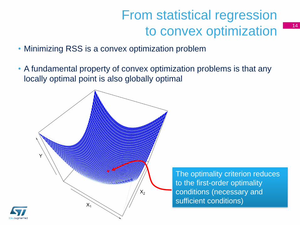
• Minimizing RSS is a convex optimization problem

• A fundamental property of convex optimization problems is that any

locally optimal point is also globally optimal

14

The optimality criterion reduces

to the first-order optimality

conditions (necessary and

sufficient conditions)

Data Analysis and

Data Set Generation

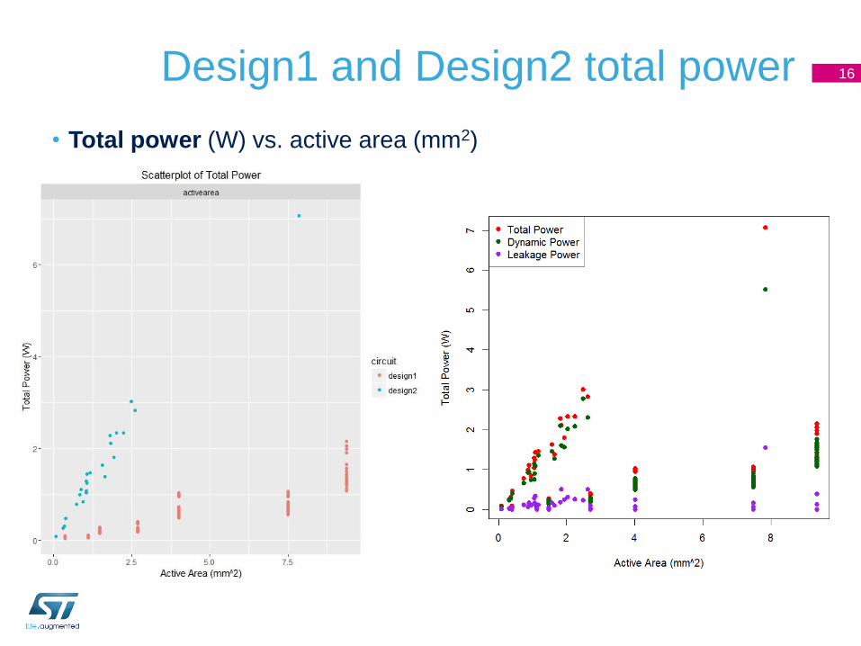
Design1 and Design2 total power

• Total power (W) vs. active area (mm2)

16

Power distribution

• In order to apply linear regression the dependent variable (total or dynamic

power) needs to be (approximately) normally distributed

• Both Design1 (test set) total and dynamic power show a positively skewed

distribution

17

Power transformations:

Box-Cox transformation

• In statistical learning power transformations correspond to a family of

functions that are applied to create a rank-preserving transformation

of data using power functions

• This class of data transformation techniques are used to:

• Stabilize variance

• Make the data more normal distribution-like

• Improve the validity of measures of association such as the Pearson

correlation between variables

• The one-parameter Box-Cox transformation (1964) is defined as:

18

niY

niY

Y

i

iCoxBox

i

,,10),log(

,,10,1

Box-Cox transformation

• A linear relationship is much more evident in the Box-Cox transformed

domain

19

Expanding the training set

• To reduce the standard error we need to increase the sample size

• The sample size is the training set size, i.e., the Design1 data set

• Design1 data set includes 112 elements (16x7, where 7 is the number of

blocks)

• How do we generate statistically consistent elements to increase the

sample size?

• The new training set size is 1000 and its element values are

generated in the following way:

• Supply voltage and temperature values are randomly generated based on

a normal distribution, with the same mean value of the original Design1

data and with ±3σ values corresponding to the upper and lower values of

the original Design1 data range

• Active area values are randomly generated based on a uniform

distribution within the corresponding original Design1 data range

20

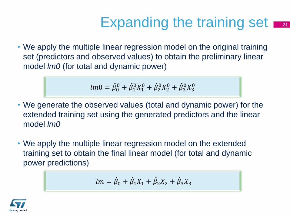
Expanding the training set

• We apply the multiple linear regression model on the original training

set (predictors and observed values) to obtain the preliminary linear

model lm0 (for total and dynamic power)

• We generate the observed values (total and dynamic power) for the

extended training set using the generated predictors and the linear

model lm0

• We apply the multiple linear regression model on the extended

training set to obtain the final linear model (for total and dynamic

power predictions)

21

𝑙𝑚0 = 𝛽00 + 𝛽1

0𝑋10 + 𝛽2

0𝑋20 + 𝛽3

0𝑋30

𝑙𝑚 = 𝛽0 + 𝛽1𝑋1 + 𝛽2𝑋2 + 𝛽3𝑋3

The framework: RStudio 22

Implementation snapshots in R 23

library(caret)library(psych)

skew(data$total)1.265956skew(data$dynamic)1.149457

boxcoxtotal = BoxCoxTrans(data$total, fudge=bcfudge1)boxcoxdynamic = BoxCoxTrans(data$dynamic, fudge=bcfudge1)data$bctotal = predict(boxcoxtotal, data$total)data$bcdynamic = predict(boxcoxdynamic, data$dynamic)

skew(data$bctotal)-0.0401338skew(data$bcdynamic)-0.03818274

Implementation snapshots in R 24

lm = lm(total~supply+temp+activearea, data=newdata)summary(lm)

## ## Call:## lm(formula = total ~ supply + temp + activearea, data = newdata)## ## Residuals:## Min 1Q Median 3Q Max ## -0.82912 -0.17663 -0.01026 0.18189 0.92597 ## ## Coefficients:## Estimate Std. Error t value Pr(>|t|) ## (Intercept) -4.841142 0.439259 -11.021 < 2e-16 ***## supply 3.016744 0.516979 5.835 7.25e-09 ***## temp 0.051388 0.006570 7.821 1.33e-14 ***## activearea 0.870906 0.008201 106.195 < 2e-16 ***## ---## Signif. codes: 0 '***' 0.001 '**' 0.01 '*' 0.05 '.' 0.1 ' ' 1## ## Residual standard error: 0.2722 on 996 degrees of freedom## Multiple R-squared: 0.92, Adjusted R-squared: 0.9197 ## F-statistic: 3816 on 3 and 996 DF, p-value: < 2.2e-16

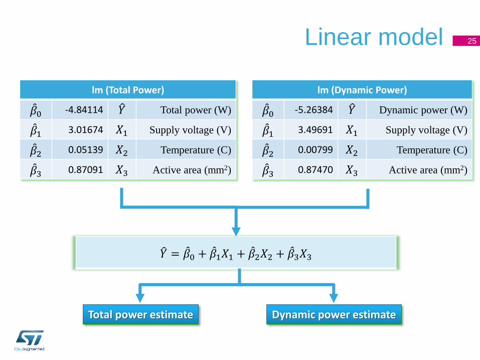
Linear model 25

lm (Total Power)

𝛽0 -4.84114 𝑌 Total power (W)

𝛽1 3.01674 𝑋1 Supply voltage (V)

𝛽2 0.05139 𝑋2 Temperature (C)

𝛽3 0.87091 𝑋3 Active area (mm2)

lm (Dynamic Power)

𝛽0 -5.26384 𝑌 Dynamic power (W)

𝛽1 3.49691 𝑋1 Supply voltage (V)

𝛽2 0.00799 𝑋2 Temperature (C)

𝛽3 0.87470 𝑋3 Active area (mm2)

𝑌 = 𝛽0 + 𝛽1𝑋1 + 𝛽2𝑋2 + 𝛽3𝑋3

Total power estimate Dynamic power estimate

Assumptions: linear relationship 26

Assumptions: residuals distributions 27

Total Power

lm(total(W)supply(V)+temp(T)+activearea(mm^2))

Dynamic Power

lm(dynamic(W)supply(V)+temp(T)+activearea(mm^2))

Frequency and Switching Activity

Scaling

Correlation analysis

• Pearson correlation coefficient between random variables Y and X:

• When |r|==1 there is a perfect linear correlation between xi and yi

29

𝑟 = 𝑥𝑖 − 𝑥 ∙ 𝑦𝑖 − 𝑦

𝑥𝑖 − 𝑥 2 𝑦𝑖 − 𝑦 2

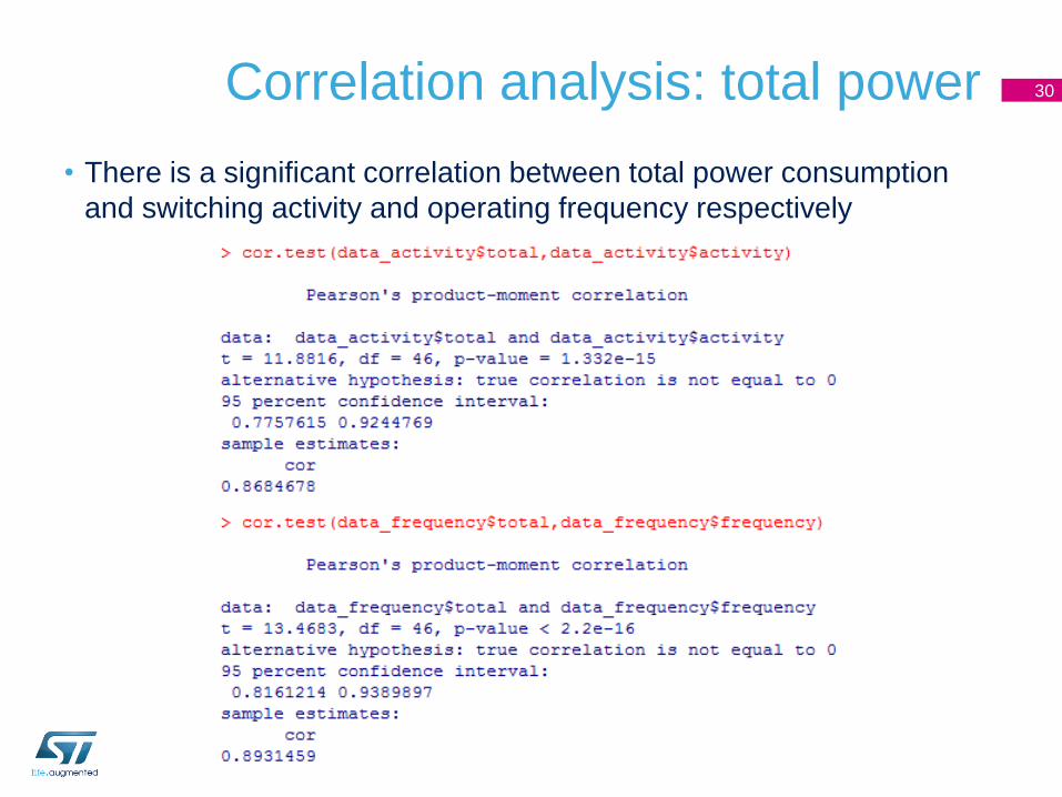
Correlation analysis: total power

• There is a significant correlation between total power consumption

and switching activity and operating frequency respectively

30

Correlation analysis: dynamic power

• There is the same level of significant correlation between dynamic

power and switching activity and operating frequency respectively

31

Correlation analysis: leakage power

• There is no significant correlation between leakage power and

switching activity and operating frequency respectively

32

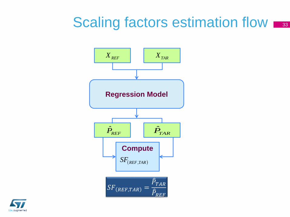
Scaling factors estimation flow 33

REFX TARX

Regression Model

REFP̂ TARP̂

Compute

TARREFSF ,

𝑆𝐹 𝑅𝐸𝐹,𝑇𝐴𝑅 = 𝑃𝑇𝐴𝑅 𝑃𝑅𝐸𝐹

Putting It All Together

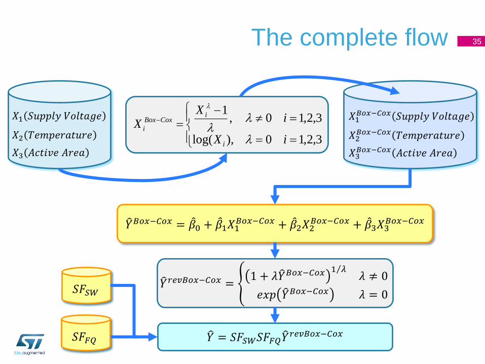
The complete flow 35

𝑌𝑟𝑒𝑣𝐵𝑜𝑥−𝐶𝑜𝑥 = 1 + 𝜆 𝑌𝐵𝑜𝑥−𝐶𝑜𝑥

1 𝜆𝜆 ≠ 0

𝑒𝑥𝑝 𝑌𝐵𝑜𝑥−𝐶𝑜𝑥 𝜆 = 0

𝑌 = 𝑆𝐹𝑆𝑊𝑆𝐹𝐹𝑄 𝑌𝑟𝑒𝑣𝐵𝑜𝑥−𝐶𝑜𝑥

𝑌𝐵𝑜𝑥−𝐶𝑜𝑥 = 𝛽0 + 𝛽1𝑋1𝐵𝑜𝑥−𝐶𝑜𝑥 + 𝛽2𝑋2

𝐵𝑜𝑥−𝐶𝑜𝑥 + 𝛽3𝑋3𝐵𝑜𝑥−𝐶𝑜𝑥

𝑆𝐹𝑆𝑊

𝑆𝐹𝐹𝑄

𝑋2 𝑇𝑒𝑚𝑝𝑒𝑟𝑎𝑡𝑢𝑟𝑒

𝑋1 𝑆𝑢𝑝𝑝𝑙𝑦 𝑉𝑜𝑙𝑡𝑎𝑔𝑒

𝑋3 𝐴𝑐𝑡𝑖𝑣𝑒 𝐴𝑟𝑒𝑎

𝑋2𝐵𝑜𝑥−𝐶𝑜𝑥 𝑇𝑒𝑚𝑝𝑒𝑟𝑎𝑡𝑢𝑟𝑒

𝑋1𝐵𝑜𝑥−𝐶𝑜𝑥 𝑆𝑢𝑝𝑝𝑙𝑦 𝑉𝑜𝑙𝑡𝑎𝑔𝑒

𝑋3𝐵𝑜𝑥−𝐶𝑜𝑥 𝐴𝑐𝑡𝑖𝑣𝑒 𝐴𝑟𝑒𝑎

3,2,10),log(

3,2,10,1

iX

iX

X

i

iCoxBox

i

Model Testing and

Experimental Results

Design2 SoC power results:

statistical estimation vs. sign-off analysis 37

*ptpx results extracted from DCG DAP Design Methodology & Support report of April 1st, 2014

model ptpx estimate CI.lower CI.upper ptpx estimate CI.lower CI.upper

lm 69.4800 61.2754 46.9519 79.9685 59.8500 56.4947 43.7499 72.9523

lm err(%)

Total Power (W) Dynamic Power (W)

-11.81% -5.61%

0.00

20.00

40.00

60.00

80.00

100.00

1

Total Power (W)

CI.upper ptpx lm estimate CI.lower

0.00

10.00

20.00

30.00

40.00

50.00

60.00

70.00

80.00

1

Dynamic Power (W)

CI.upper ptpx lm estimate CI.lower

Summary

• The statistical model for power estimation yields power (total and dynamic)

predicted values in good agreement with observed (sign-off power analysis)

values both for Design1 and Design2 SoCs

• The observed value (i.e., the sign-off “true” value) falls within the confidence

intervals obtained with the statistical learning approach most of the times

• The statistical model shows a comparable good performance on both training

and test designs (very different in terms of active area, frequency, switching

activity, and power consumption)

• The proposed statistical model has been implemented in R

• Results obtained with R have been validated against commercial mathematical

frameworks like Mathematica and Matlab

• These techniques can be implemented in a Excel spreadsheet and can

effectively complement deterministic RFQ estimations

38

And then … 39

Sure, but there still is a question that puzzles me …

Because it is based on statistics …

Andrzej J. Strojwas

CMU Dept. of ECE

Keithley Professor

… and statistics it’s not so

profound …

But we are all engineers and

we have to solve problems

Doomed by the Black Swan

• We have to accept the hidden laws of Probability to model uncertainty

40

Bad things may happen to good chips

A Black Swan is a highly improbable event

with three principal characteristics:1. It is unpredictable2. It carries a massive impact3. After the fact, we concoct an explanation

that makes it appear less random, and more predictable, than it was

Doomed by the Black Swan

• In his best-seller book “The Black Swan”, Nassim N. Taleb argues that

in general statistics makes little sense (if any at all)

41

The Black Swan, 2007

Nassim N. Taleb

“When you develop your opinions on the basis of weak evidence, you will have difficulty interpreting subsequent information that contradicts these opinions, even if this new information is obviously more accurate.”

Doomed by the Black Swan

• Most of this stuff (i.e., statistical learning) by and large is based on the

underlying assumption of Gaussian normal distributions

• Everything looks like a bell curve and all curves look like bells

• For bell-like distributions the improbable is inconsequential and of low impact

• A visual presentation of a bell curve as histogram masks the contribution of remote

events (points to far right or far left of the center)

• Gaussian distributions work well only in Mediocristan

• In Mediocristan everything is constrained by boundary conditions

• Random variations exist in Mediocristan and can be described by Gaussian

distributions (the bell curve or other distributions with a family resemblance to it)

• In such probability distributions no single value of an attribute can greatly affect the

sum of all values in the distribution. The most extreme attribute values do not

materially affect the mean value of a distribution

• An individual Black Swan event almost never occurs because its probability,

according to Gaussian models, is so low

42

Doomed by the Black Swan

• But unfortunately we also live in Extremistan, where variations within

distributions are far less constrained than in Mediocristan

• Distributions have very large or very small extreme values relatively frequently

• Those extreme values often affect the sum of attribute values in a sample

distribution, and the mean value of such distributions

• The probability of occurrence of extreme values varies greatly from Gaussian

models

• Many distributions in Extremistan do not fit any known models well

• Since extreme occurrences can greatly affect statistical properties of distributions

from Extremistan, it is hard, in contrast with data from Mediocristan, to make

reliable inferences from sample data

43

A few questions

• Does the presented approach for power consumption estimation

based on statistical learning techniques sound convincing?

• Do you see any fundamental flaw or limitation in this work?

• Did I missed/overlooked some trivial and critical issue?

• Should I worry about Extremistan, or should I safely stay in Mediocristan?

• What do you suggest to make it right?

• Is there any open point to analyze?

• Are there better models or techniques?

44

45