Page 1
Arab Academy for Science and Technology and Maritime Transport
College of Engineering & Technology
Electrical and Control
Power Quality Analysis of a Grid Connected PV System
M.Sc. thesis
By:
Eng. Basem Abd-El Hamid Rashad Abd-El Razek
This Thesis is submitted to the Faculty of Engineering- Arab Academy for Science and
Technology and Maritime Transport in Partial Fulfillments of the Requirements for The
Degree of Master of Science in Electrical and Control Engineering
Supervised by:
Prof Dr. Almoataz Y. Abdelaziz Department of Electrical Power & Machines
Faculty of Engineering, Ain Shams University
Dr. Hadi Maged El- Helw
Department Electrical Power and Computer Control
Arab Academy for Science and Technology
Cairo 2014
Page 2
Arab Academy for Science and Technology and Maritime Transport
College of Engineering & Technology
Electrical and Control
Power Quality Analysis of a Grid Connected PV System
M.Sc. thesis
By:
Eng. Basem Abd-El Hamid Rashad Abd-El Razek
This Thesis is submitted to the Faculty of Engineering- Arab Academy for Science and
Technology and Maritime Transport in Partial Fulfillments of the Requirements for The
Degree of Master of Science in Electrical and Control Engineering
Supervised by:
Prof Dr. Almoataz Y. Abdelaziz Dr. Hadi Maged El- Helw Supervisor Supervisor
------------------------------- -----------------------------
Examination committee:
Prof Dr. Ahmed Abd- Elsattar Prof Dr. Said M. Wahsh Examiner Examiner
------------------------------- -------------------------------
Cairo 2014
Page 3
STATEMENT
This thesis is submitted to Arab Academy for Science and Technology and
Maritime Transport in Partial Fulfillments of the Requirements for M.Sc. degree
in Electrical and Control Engineering. The included work in this thesis has been
carried out by the author at the Electrical and Control department, Arab
Academy. No part of this thesis has been submitted for a degree or a
qualification at other university or institute.
Name: Basem Abd-El Hamid Rashad Abd-El Razek
Signature:
Date: / /
DEDICATION
To my parents, my brothers, wife, and
lovely kids
Basem Abd El-hamid Rashad Abd-el razek
Page 4
I
ACKNOWLEDGMENTS
At the beginning, I thank ALLAH for giving me the strength
and health to let this work see the light.
I wish to express my deepest gratitude to my advisors, Prof Dr. Almoataz Y.
Abdelaziz & Dr. Hadi Maged El- Helw , for his professional assistance,
support, advice and guidance throughout my thesis, and to my discussion
committee, Prof Dr. Ahmed Abd- Elsattar, And Prof Dr. Said M. Wahsh for
their acceptance to discuss my thesis.
Many thanks for head of Electrical and Control Department, Prof Dr. Rania
El- Sharkawy, for their support and cooperation.
I would also like to extend my gratitude to my family, my brothers, and my
wife, for providing all the preconditions necessary to complete my studies. They
have been always behind me throughout my academic career.
I am extremely grateful and thankful to my wife and my lovely kids Malak &
Ahmed for giving me their support, love and encouragement.
Page 5
II
Abstract
Power Quality Analysis of a Grid Connected PV System
Recently, the use of a grid-connected photovoltaic (PV) system has increased in order to
meet the rising demand of electrical energy. This needs to improve the materials and methods
used to harness this power source. Several approaches are proposed in order to accomplish the
maximum power point tracking for a PV array such as; Perturb and Observe, Incremental
Conductance, open circuit voltage, short circuit current, fuzzy or neural based etc. Among all
of these techniques those based on Artificial Inelegance are very efficient nevertheless they are
more complicated. The controller may be conventional or intelligent such as Fuzzy Logic
Controller (FLC). FLCs have the advantage to be relatively simple to design as they do not
require the knowledge of the exact model and work well for nonlinear system. The
advantage of FLC is that the linguistic system definition becomes the control algorithm.
In this thesis, a PV model is used to simulate actual PV arrays behavior, and then the
performance of three maximum power point tracking techniques is evaluated for grid-
connected PV system in order to control the DC-DC converter. The methods used for
comparative study are (i) Perturb & observe (P&O) (ii) Incremental conductance technique
(ICT) and (iii) Fuzzy logic based (FLC). Voltage-Sourced Converter (VSC) technique is
applied on the three phase inverter so that the output voltage of the converter remains
constant at any required set point which facilitates the maximum power point process.
A grid-connected complete PV model is generated to simulate the actual life case. The
proposed FLC algorithm is compared with the conventional hill climbing based techniques.
The grid disturbances effects on a grid connected PV array were studied while considering
different maximum power point tracking algorithms. The grid disturbances involved in this
thesis are the different types of faults, voltage sag, and voltage swell. A comparative study of
the grid disturbances effect on the three maximum power point tracking algorithms is
discussed.
Page 6
III
Simulation results show that the proposed FLC algorithm gives least oscillations around
the final operating point and gives faster response than the conventional hill climbing based
techniques under rapid variations of operating conditions. Also the VSC inverter control
scheme shows fast response and that facilitates the maximum power tracking process with the
grid connection.
Furthermore, the simulation results under steady state condition show the effectiveness of
the MPPT on increase the output power of the PV array for the three techniques. However the
FLC algorithm offers accurate and faster response compared to the others. The simulation
results under transient conditions show that, the output power injected to grid from PV array
is approximately constant while utilizing the proposed FLC and the PV system can still
connect to grid and deliver power to grid without any damage to the inverter switches.
Page 7
IV
Contents
Abstract ........................................................................................................................................................ II
Contents ...................................................................................................................................................... IV
List of Tables ............................................................................................................................................. VII
List of Figures ........................................................................................................................................... VIII
List of Abbreviations ................................................................................................................................... X
CHAPTER 1 ................................................................................................................................................ 1
INTRODUCTIOIN ...................................................................................................................................... 1
1.1 INTRODUCTION ............................................................................................................................. 2
1.2 MOTIVATION .................................................................................................................................. 3
1.3 OBJECTIVES .................................................................................................................................... 3
1.4 OUTLINE OF THE THESIS ............................................................................................................ 4
CHAPTER 2 ................................................................................................................................................ 6
INTRODUCTION TO PHOTOVOLTAIC ENERGY ................................................................................ 6
2.1 BACKGROUND ............................................................................................................................... 7
2.1.1 Renewable Energy .................................................................................................................... 7
2.1.2 Solar Energy ............................................................................................................................. 9
2.1.2.1 The Photovoltaic Resource .......................................................................................... 9
2.2 PHOTOVOLTAIC BACKGROUND .............................................................................................. 10
2.3 PRINCIPLE OF PHOTOVOLTAIC SYSTEMS ............................................................................. 10
2.4 TYPES OF PV CELLS .................................................................................................................... 11
2.5 EQUIVALENT CIRCUIT AND MATHEMATICAL MODEL ..................................................... 13
2.6 NON LINEAR CHARACTERISTICS VERIFICATION ............................................................... 15
2.7 PV APPLICATIONS ....................................................................................................................... 18
2.8 ADVANTAGES OF PV SYSTEMS ............................................................................................... 19
2.9 SUMMARY ..................................................................................................................................... 20
CHAPTER 3 .............................................................................................................................................. 21
MPPT ALGORITHMS .............................................................................................................................. 21
3.1 REVIEW OF MAXIMUM POWER POINT TRACKING ............................................................. 22
3.2 MAXIMUM POWER POINT TRACKING .................................................................................... 23
3.3 CONTROL ALGORITHMS ............................................................................................................ 24
Page 8
V
3.3.1 Hill Climbing Method ............................................................................................................. 24
3.3.1.1 Perturb and Observe method (P&O) ......................................................................... 24
3.3.1.2 Incremental Conductance method (ICT) ................................................................... 26
3.3.2 Proposed Fuzzy Logic Controller Based Algorithm (FLC) .................................................... 28
3.3.2.1 MPPT Fuzzy Logic Controller .................................................................................. 28
3.4 DC-DC CONVERTERS .................................................................................................................. 32
3.4.1 Boost Converters..................................................................................................................... 32
3.5 VOLTAGE SOURCE CONVERTER (VSC) .................................................................................. 33
3.5.1 DQ Transformation ................................................................................................................. 34
3.5.2 Phase Locked Loop (PLL) ...................................................................................................... 35
3.5.3 Vector Control ........................................................................................................................ 35
3.5.3.1 DC-Voltage Controller .............................................................................................. 36
3.5.3.2 Inner Current Controller ............................................................................................ 37
3.6 SINUSOIDAL PULSE WIDTH MODULATION (SPWM) ........................................................... 38
3.7 SUMMARY ..................................................................................................................................... 39
CHAPTER 4 .............................................................................................................................................. 40
POWER QUALITY TERMS AND DEFINITIONS ................................................................................. 40
4.1 INTRODUCTION ........................................................................................................................... 41
4.2 DEFINITION OF POWER QUALITY ........................................................................................... 41
4.3 POWER QUALITY DISTURBANCES CLASSIFICATION ........................................................ 42
4.3.1 Transients ................................................................................................................................ 43
4.3.2 Short-Duration Variations ....................................................................................................... 43
4.3.2.1 Voltage Sag (Dip) ...................................................................................................... 43
4.3.2.2 Voltage Swell ............................................................................................................ 44
4.3.2.3 Voltage Interruption .................................................................................................. 44
4.3.3 Long-Duration Variations ....................................................................................................... 44
4.3.3.1 Over-voltage .............................................................................................................. 44
4.3.3.2 Under-voltage ............................................................................................................ 44
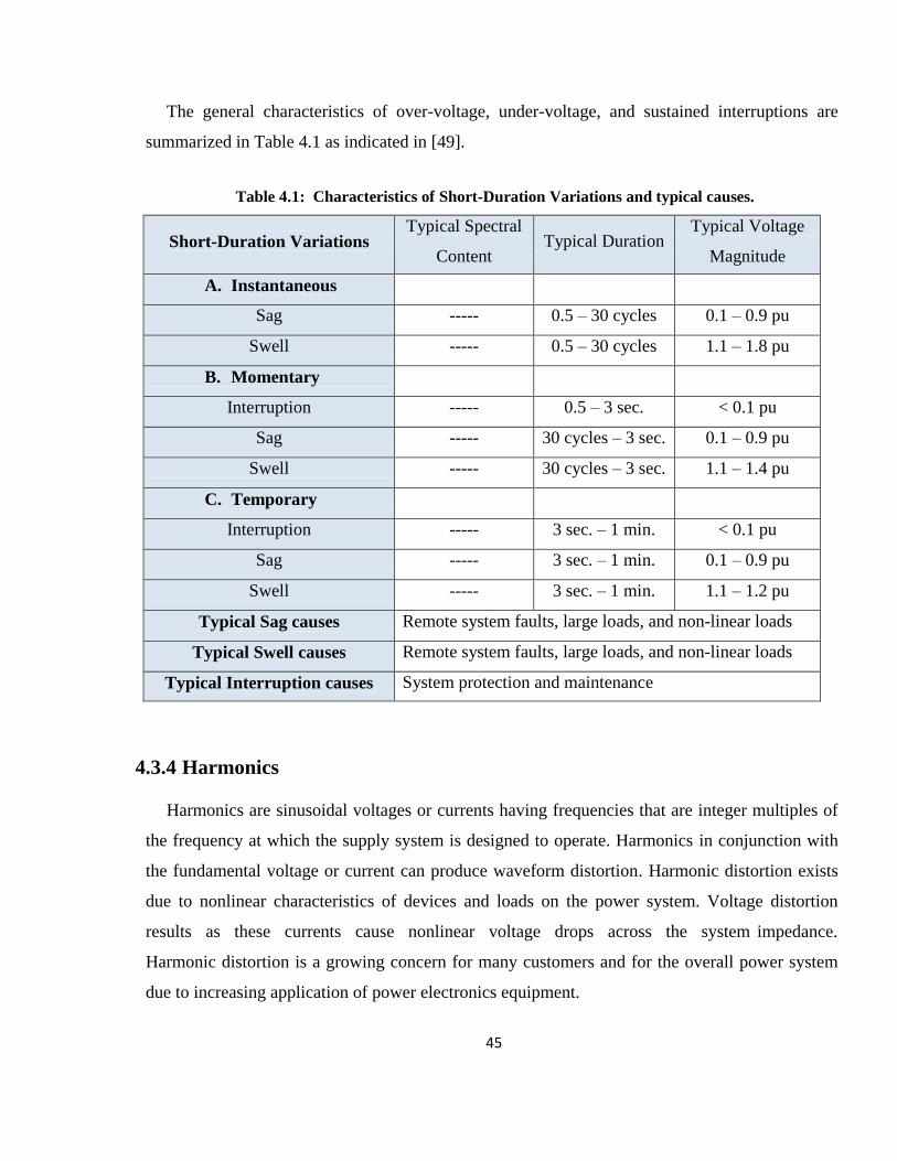
4.3.4 Harmonics ............................................................................................................................... 45
4.4 SIGNAL ANALYSIS ...................................................................................................................... 46
4.5 CONCLUSION ................................................................................................................................ 47
Page 9
VI
CHAPTER 5 SIMULAION RESULTS ..................................................................................................... 48
5.1 INTRODUCTION ........................................................................................................................... 49
5.2 SYSTEM UNDER STUDY ............................................................................................................. 49
5.3 PV MODELING FOR SIMULATION ............................................................................................ 50
5.4 BOOST CONVERTER MODEL .................................................................................................... 53
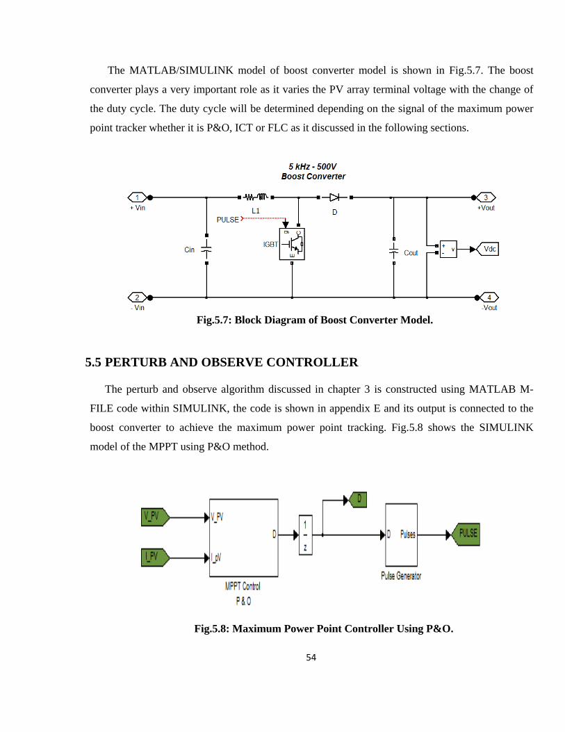
5.5 PERTURB AND OBSERVE CONTROLLER ............................................................................... 54
5.6 INCREMENTAL CONDUCTANCE CONTROLLER ................................................................... 55
5.7 PROPOSED FUZZY LOGIC CONTROLLER ............................................................................... 55
5.8 INVERTER CONTROLLER ........................................................................................................... 57
5.9 SIMULATION RESULTS............................................................................................................... 58
5.9.1 STEADY STATE ANALYSIS .............................................................................................. 59
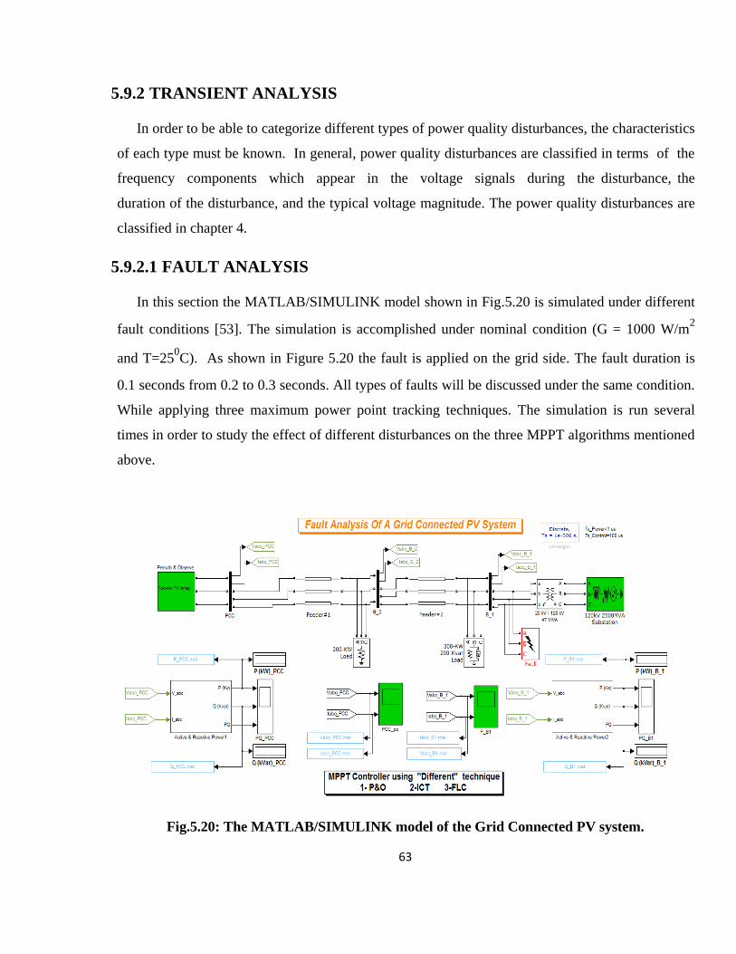
5.9.2 TRANSIENT ANALYSIS ..................................................................................................... 63
5.9.2.1 FAULT ANALYSIS ................................................................................................. 63
5.9.2.2 SAG ANALYSIS ...................................................................................................... 68
5.9.2.3 SWELL ANALYSIS ................................................................................................. 70
5.10 CONCLUSION .............................................................................................................................. 71
CHAPTER 6 CONCLUSION AND SCOPE FOR FUTURE WORK ...................................................... 72
6.1 CONCLUSION ................................................................................................................................ 73
6.2 SCOPE FOR FUTURE WORK ....................................................................................................... 74
REFERENCES........................................................................................................................................... 75
REFERENCES ....................................................................................................................................... 76
APPENDICES ........................................................................................................................................... 79
APPENDICES ....................................................................................................................................... 80
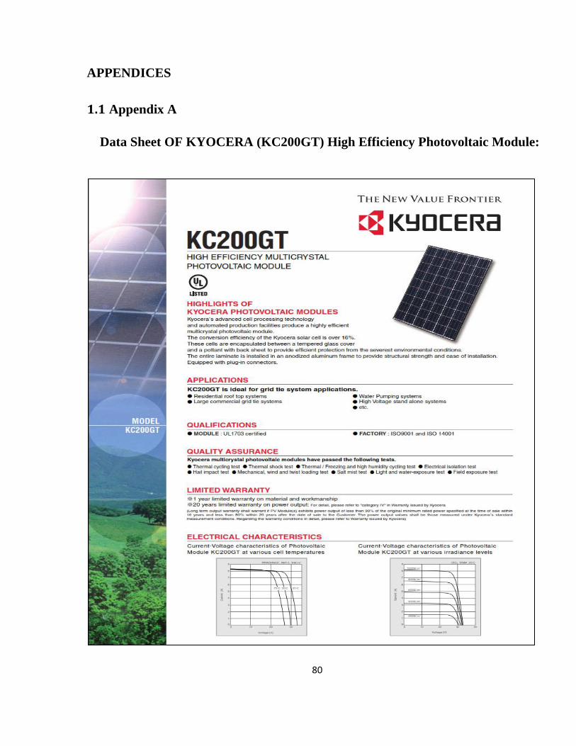
1.1 Appendix A ...................................................................................................................................... 80
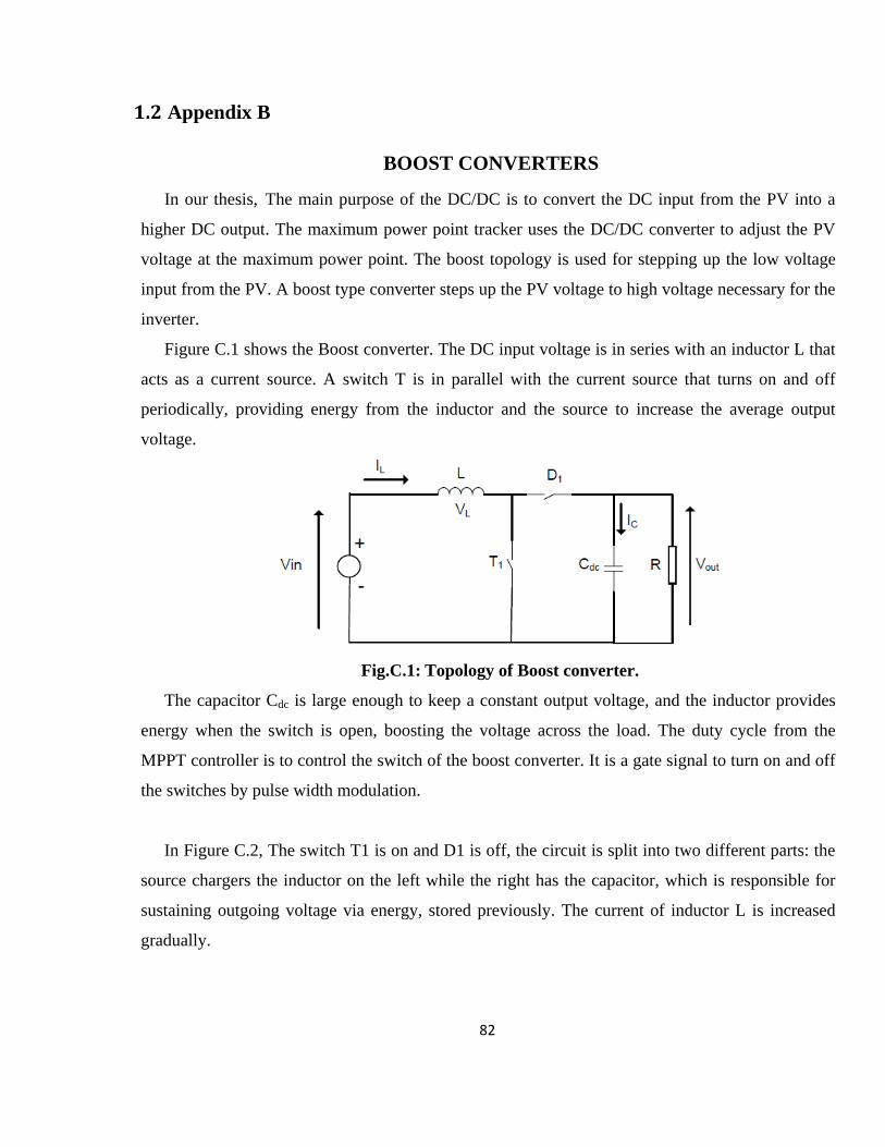
1.2 Appendix B ...................................................................................................................................... 82
1.3 Appendix C ...................................................................................................................................... 85
1.4 Appendix D ...................................................................................................................................... 86
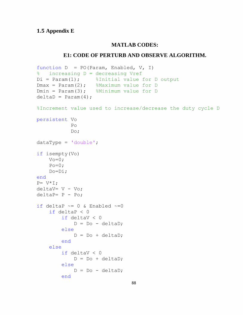
1.5 Appendix E ...................................................................................................................................... 88
PUBLICATION OUT OF THIS THESIS ............................................................................................. 91
Page 10
VII
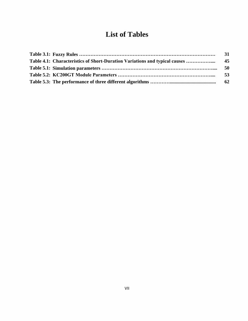
List of Tables
Table 3.1: Fuzzy Rules ………………………………………………………………………… 31
Table 4.1: Characteristics of Short-Duration Variations and typical causes …………….... 45
Table 5.1: Simulation parameters …………………………………………………………….... 50
Table 5.2: KC200GT Module Parameters ………………………………………………….... 53
Table 5.3: The performance of three different algorithms …………...................................... 62
Page 11
VIII
List of Figures
Fig.2.1: Renewable energy share of global electricity production, 2013 [6]…………….. 8
Fig.2.2: Total World Capacity of PV (1995-2012) [6]……………………………………... 9
Fig.2.3: Principle of Photovoltaic cells …………………………………………………….. 11
Fig.2.4: Mono-crystalline Solar Panels……………………………………………………... 12
Fig.2.5: Polycrystalline Solar Panels……………………………………………………….. 12
Fig.2.6: Amorphous Solar Panels…………………………………………………………... 13
Fig.2.7: Equivalent Circuit of PV module………………………………………………….... 13
Fig.2.8: I-V and P-V characteristics of the PV module at constant temperature 25°C and
various irradiances…………………………………………………………………..
15
Fig.2.9: I-V and P-V characteristics of the PV module under constant irradiance and
different temperature………………………………………………………………..
16
Fig.2.10: I-V and P-V characteristics at constant temperature 25oC and various
irradiances for the PV array………………………………………………………...
17
Fig.2.11: Typical grid - connected PV systems ……………………………………………..... 18
Fig.3.1: P-V characteristics of a practical PV array showing MPP……………………….. 22
Fig.3.2: Maximum Power Point Tracker (MPPT) system as a block diagram…………… 23
Fig.3.3: Flowchart for maximum power point tracking for (P&O) Algorithm…………… 25
Fig.3.4: Flow Chart for maximum power point tracking for (ICT) Algorithm…………… 27
Fig.3.5: Block diagram of Proposed Fuzzy (FLC) Based Tracking……………………….. 28
Fig.3.6: Power-voltage characteristic of a PV module……………………………………... 29
Fig.3.7: Membership functions for input variable (E)……………………………………. 30
Fig.3.8: Membership functions for input variable (CH_E)………………………………. 30
Fig.3.9: Membership functions for output variable (D)…………………………………..... 30
Fig.3.10: Boost Converter Circuit Diagram………………………………………………...... 32
Fig.3.11: Functional control diagram of VSC using vector control……………………….... 33
Fig.3.12: Transformation of axes for vector control……………………………………….. 34
Fig.3.13: Schematic diagram of the phase locked loop (PLL)……………………………… 35
Fig.3.14: Simulink Model of the DC-Voltage Controller…………………………………… 37
Fig.3.15: Total converter control scheme.…………………………………………………… 37
Fig.3.16: Pulse width modulation waveforms………………………………………………. 38
Fig.5.1: Block diagram of the grid connected photovoltaic system………………………... 49
Fig.5.2: Simulink Model for Evaluating ……………………………………………….. 51
Fig.5.3: Simulink Model for Evaluating ………………………………………………... 51
Fig.5.4: Mathematical Model Implementation for Model Current …………………..... 52
Page 12
IX
Fig.5.5: Simulation of the Photovoltaic Module…………………………………………..... 52
Fig.5.6: PV model Subsystem………………………………………………………………... 53
Fig.5.7: Block Diagram of Boost Converter Model………………………………………… 54
Fig.5.8: Maximum Power Point Controller Using P&O…………………………………… 54
Fig.5.9: Maximum Power Point Controller Using ICT……………………………………. 55
Fig.5.10: Controlling the PV power using FLC……………………………………………… 55
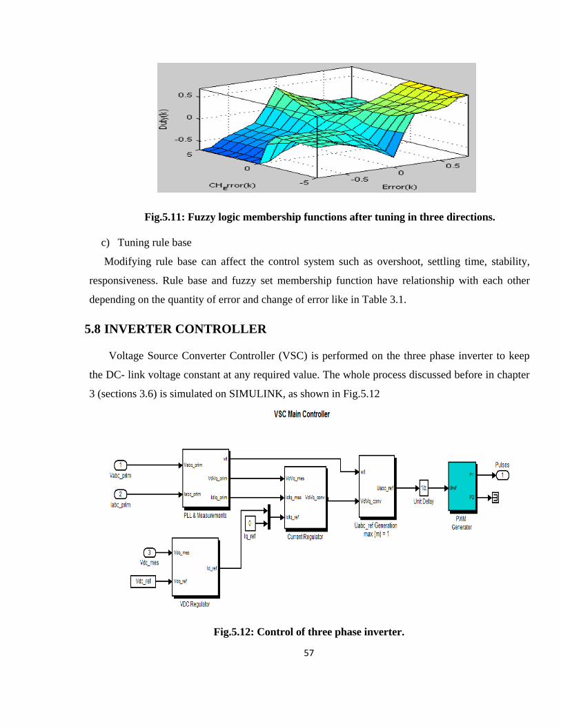
Fig.5.11: Fuzzy logic membership functions after tuning in three directions……………… 57
Fig.5.12: Control of three phase inverter…………………………………………………….. 57
Fig.5.13: DC-link voltage VS Reference voltage……………………………………………… 58
Fig.5.14: The MATLAB/ Simulink model of the system under investigation………………. 58
Fig.5.15: Voltage, Current and Power Output of PV array with MPPT Based P&O …….. 59
Fig.5.16: Voltage, Current and Power Output of PV array with MPPT Based ICT ……… 60
Fig.5.17: Voltage, Current and Power Output of PV array with MPPT Based FLC……… 61
Fig.5.18: The output power of the PV array using the three different algorithms
at constant irradiance………………………………………………………………..
61
Fig.5.19: The output power of the PV array using the three different algorithms
at variable irradiance……………………………………………………………….
62
Fig.5.20: The MATLAB/SIMULINK model of the Grid Connected PV system…………... 63
Fig.5.21: Output Voltage and current at the PCC with 1L-G fault………………………… 63
Fig.5.22: Output Power of the PV Array using the three different algorithms with 1LG
fault…………………………………………………………………………………...
64
Fig.5.23: Output Voltage and current at the PCC with L-L fault…………………………... 64
Fig.5.24: Output Power of the PV array using the three different algorithms with L-L
fault…………………………………………………………………………………..
65
Fig.5.25: Output Voltage and current at the PCC with L-L-G fault ………………………. 65
Fig.5.26: Output Power of The PV Array using the three different algorithms
With L-L-G fault…………………………………………………………………….
66
Fig.5.27: Output Voltage and current at Point of common coupling (PCC)
with L-L-L-G fault…………………………………………………………………
66
Fig.5.28: Output power of The PV Array using the three different algorithms
with L-L-L-G fault…………………………………………………………………..
67
Fig. 5.29: Grid Connected PV system under Sag Analysis…………………………………... 67
Fig.5.30: Output voltage and current at PCC in case of voltage decreased to 50% ………. 68
Fig.5.31: Output power of The PV Array using the three different algorithms
Under voltage sag……………………………………………………………………
68
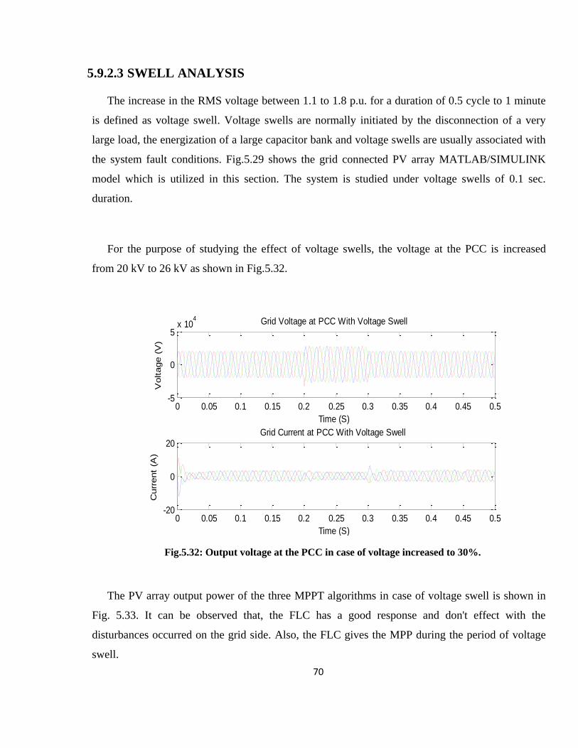
Fig.5.32: Output voltage at the PCC in case of voltage increased to 30% ………………… 69
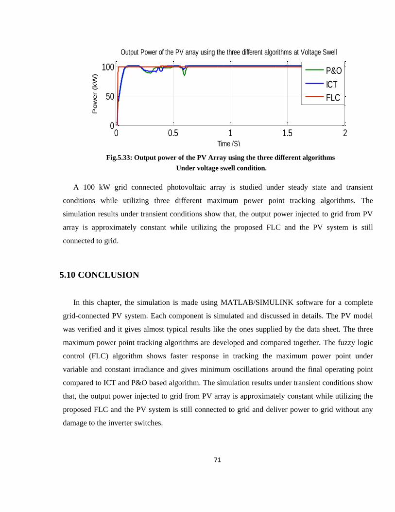
Fig.5.33: Output power of the PV Array using the three different algorithms
Under voltage swell condition……………………………………………………….
70
Page 13
X
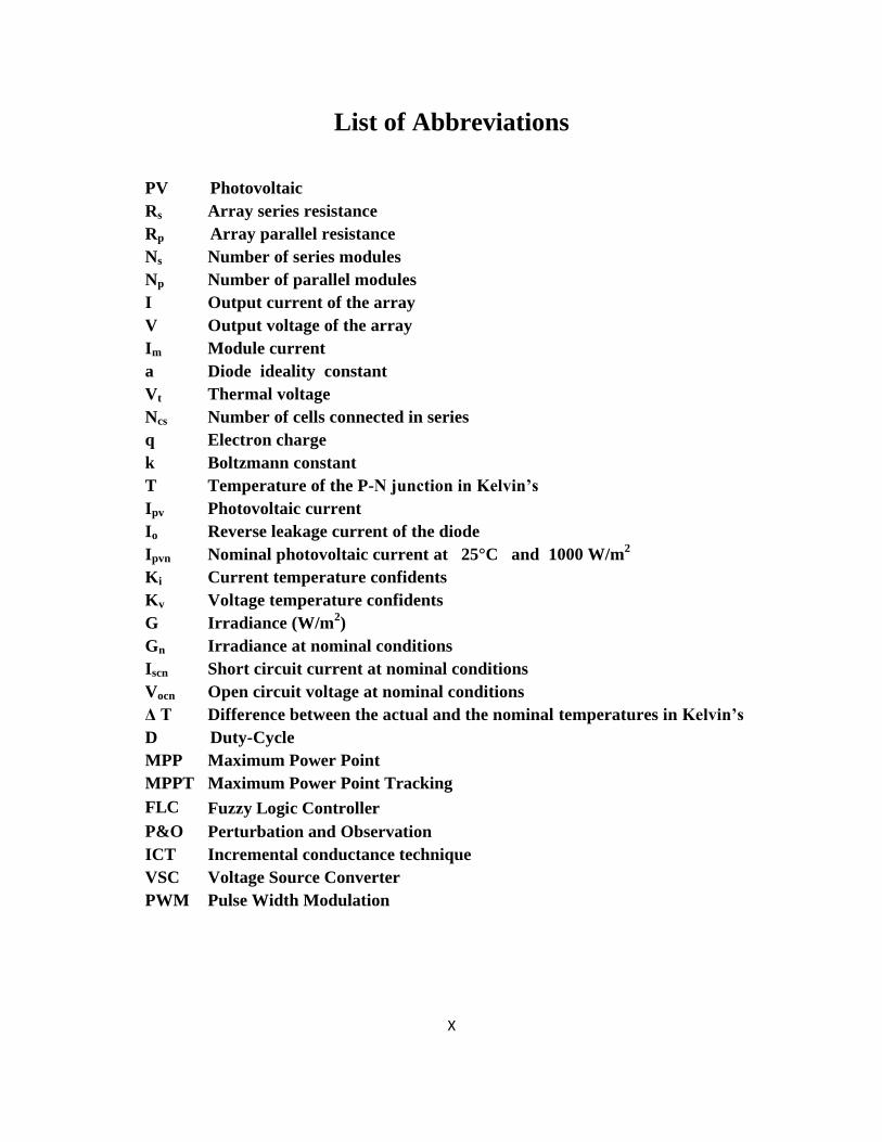
List of Abbreviations
PV Photovoltaic
Rs Array series resistance
Rp Array parallel resistance
Ns Number of series modules
Np Number of parallel modules
I Output current of the array
V Output voltage of the array
Im Module current
a Diode ideality constant
Vt Thermal voltage
Ncs Number of cells connected in series
q Electron charge
k Boltzmann constant
T Temperature of the P-N junction in Kelvin’s
Ipv Photovoltaic current
Io Reverse leakage current of the diode
Ipvn Nominal photovoltaic current at 25°C and 1000 W/m2
Ki Current temperature confidents
Kv Voltage temperature confidents
G Irradiance (W/m2)
Gn Irradiance at nominal conditions
Iscn Short circuit current at nominal conditions
Vocn Open circuit voltage at nominal conditions
Δ T Difference between the actual and the nominal temperatures in Kelvin’s
D Duty-Cycle
MPP Maximum Power Point
MPPT Maximum Power Point Tracking
FLC Fuzzy Logic Controller
P&O Perturbation and Observation
ICT Incremental conductance technique
VSC Voltage Source Converter
PWM Pulse Width Modulation
Page 14
1
CHAPTER 1
INTRODUCTIOIN
Page 15
2
1.1 INTRODUCTION
The usage of the grid-connected photovoltaic (PV) system has improved in order to meet the
rising request of electrical energy. The non-linear characteristics of the PV array and the
dependency of its output power on the array terminal voltage for the same environmental
conditions make the task of efficiently utilizing the power generated by PV array challenging.
When many such PV modules are connected in series and parallel combinations we get a PV array,
that suitable for obtaining higher power output.
The applications for PV energy are increased, and that need to improve the materials and
methods used to harness this power source. Main factors that affect the efficiency of the collection
process are PV efficiency, intensity of source radiation and storage techniques. The efficiency
of a PV is limited by materials used in PV manufacturing. It is particularly difficult to make
considerable improvements in the performance of the cell, and hence controls the efficiency of the
overall collection process. Therefore, the increase of the intensity of radiation received from the
sun is the most attainable method of improving the performance of solar power.
There are two major methodologies for maximizing power extraction in solar systems. They are
sun tracking, maximum power point (MPP) tracking or both. These methods need controllers which
may be intelligent such as fuzzy logic controller or conventional controller such as Perturb &
Observe method and Incremental Conductance method. The advantage of the fuzzy logic control is
that it does not strictly need any mathematical model of the plant. It is based on plant operator
experience, and it is very easy to apply. Hence, many complex systems can be controlled
without knowing the exact mathematical model of the plant. In addition, fuzzy logic simplifies
dealing with nonlinearities in systems. The most popular method of implementing fuzzy controller
is using a general-purpose microprocessor or microcontroller.
Later on in this thesis, three tracking algorithms are studied and compared on steady-state and
transient conditions. The first algorithm is based on P&O, the second is based on ICT and the third
is based on FLC algorithm. Also a complete grid connected structure is proposed along with a DC-
AC inverter control technique based on VSC (Voltage-Sourced Converter).
Page 16
3
1.2 MOTIVATION
Renewable energy is the energy which is collected from the natural resources like sunlight,
wind, tides, geothermal heat etc. As these resources can be naturally replaced, for all practical
purposes, these can be considered to be limitless unlike the narrowing conventional fossil fuels.
The global energy crisis has provided a renewed impulsion to the growth and development
of clean and renewable energy sources. Another advantage of utilizing renewable resources over
conventional methods is the significant reduction in the level of pollution associated. The cost of
conventional energy is rising and solar energy has emerged to be a promising alternative. They are
abundant, pollution free, distributed throughout the earth and recyclable. PV arrays consist of
parallel and series combination of PV cells that are used to generate electrical power depending
upon the atmospheric specifies (e.g. solar insolation and temperature). Nowadays, fuzzy logic
controllers have an efficient performance over the traditional controller researches especially in
nonlinear and complex model systems. Modern manufactures began to apply these technologies in
their applications instead of the traditional ones, due to the low cost and widely features
available in these controllers.
In Egypt we have a big problem in electrical power generation, since our sources don't cover all
consumer requirements, electrical power have high cost and many daily interruptions, so we need
clean renewable energy sources such as solar energy. This motivated to implement FLC techniques
to control the MPP of a grid connected photovoltaic systems.
1.3 OBJECTIVES
The main objectives of the thesis are building an FLC for maximizing the power output of the
solar arrays and comparing the FLC technique with the hill climbing techniques. Then the grid
disturbances effects on a grid connected PV array were studied while considering different
maximum power point tracking algorithms.
The specific objectives include:
Modeling of the PV array using the MATLAB/SIMULINK.
Page 17
4
Using model to obtain the MPPT of grid connected PV array considering different
techniques.
P&O method.
ICT method.
Fuzzy logic method.
The grid disturbances effects on a grid connected PV array are studied while considering
different maximum power point tracking algorithms. The grid disturbances involved in this
thesis are the different types of :
Faults.
Voltage sags.
Voltage swells.
1.4 OUTLINE OF THE THESIS
The thesis consists of six chapters in which the MPPT problem is discussed in details and the proposed
control schemes are fully explained. Also the grid disturbances effects on a grid connected PV array are
studied while considering different maximum power point tracking algorithms. The grid disturbances
involved in this thesis are the different types of faults, voltage sag, and voltage swell. A comparative study
of the grid disturbances effect on the three maximum power point tracking algorithms is discussed.
Chapter two handles some basic principles of solar energy and especially on PV's and their types ,
equivalent circuits and characteristics. From which the MPPT problem originates.
Chapter three discusses the MPPT problem in details and shows different MPPT algorithms. Three
MPPT techniques are discussed in details in this chapter (P&O, ICT and the proposed FLC) and also the
role of DC-DC converters and DC-AC inverters is explained.
Chapter four In light of this definition of power quality, this chapter provides an introduction to
the more common power quality terms. Along with definitions of the terms, explanations are
included in parentheses where necessary. This chapter also attempts to explain how power quality
factors interact in an electrical system.
Page 18
5
Chapter five shows the simulation results for the grid connected PV system using P&O algorithm,
ICT algorithm and the proposed FLC method, and the comparison between these algorithms is discussed.
The grid disturbances effects on a grid connected PV array are studied while considering different
maximum power point tracking algorithms. All the simulations are made using the
MATLAB/SIMULINK computer software.
Finally in chapter six, an overall conclusion is presented and the outcomes of the thesis are stated.
Page 19
6
CHAPTER 2
INTRODUCTION TO
PHOTOVOLTAIC ENERGY
Page 20
7
2.1 BACKGROUND
Renewable energy sources perform a significant role in electric power generation. There are
various renewable sources which used for electric power generation, such as wind energy, PV
energy, geothermal etc. P V energy is a good choice for electric power generation, since the
PV energy is directly converted into electrical energy by photovoltaic modules. These
modules are made up of semiconductor cells. When many such cells are connected in series and
parallel combinations we get a solar PV module. The current rating of the modules increases when
the area of the individual cells is increased, and vice versa. The increase of world energy request
and the environmental concerns lead to an increase of the renewable energy production over the last
decade. Energy sources such as solar, wind or hydro became more and more popular mainly
because they produce no emissions and are limitless. PV energy is the fastest growing renewable
source with a history dating since it has been first used as power supply for space satellites. The
increased efforts in the semiconductor material technology resulted in the appearance of
commercial PV cells and consequently made the PVs an important alternative energy source [1].
One of the major advantage of PV technology is the lack of moving parts which offers the
possibility to obtain a long operating time (>20 years) and low maintenance cost. The main
drawbacks are the high manufacturing cost and low efficiency (15-20 %). As one of the most
promising renewable and clean energy resources, PV power development has been boosted by the
favorable governmental support [2].One of the most important problems facing the world today is
the energy problem. This problem is resulted from the increase of demand for electrical energy and
raised of fossil fuel prices. Another problem in the world is the global climate change has
increased. As these problems alternative technologies for producing electricity have received
greater attention. The most important solution was in finding other renewable energy resources [3],
[4].
2.1.1 Renewable Energy
Each year, the addition of persons to world will increase and the resources required to support
them will also increase. Of the resources, one of the most dynamic to support the technological
advancing population is energy.
Page 21
8
The energy crisis became transparent in the late 1900‟s and birthed the desire to find additional
energy resources to meet rising energy demands [5].One choice was to increase generation of
currently used energy sources such as nuclear, fossil fuel, etc. The other was to explore new
renewable energy alternatives. Many different renewable energy sources have appeared as feasible
solutions and each one of them has their own positive and negative attributes. As a whole,
renewable energy sources all share the fact that their fuel is primarily free and they produce
minimal to no waste. These factors are the main motivation for countries to begin incorporating
renewable into their energy collection.
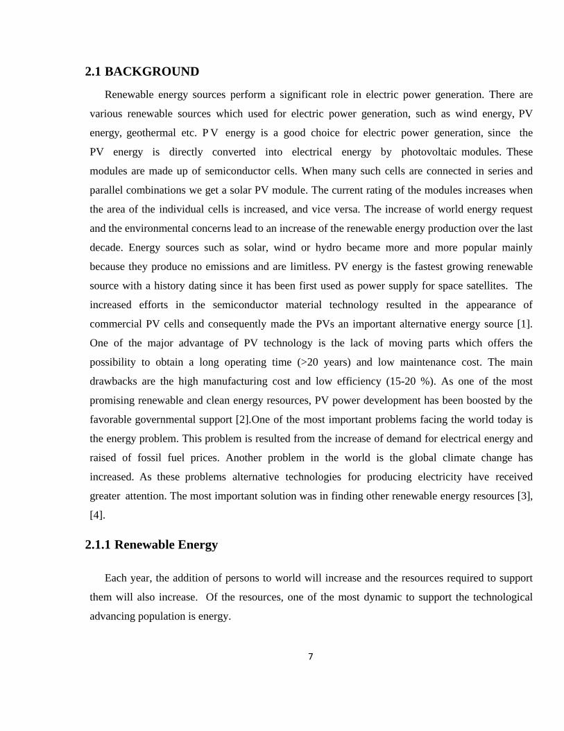
A predictable 19% of global energy consumption in 2013 was supplied by renewable energy
[6]. One more analysis of where the world‟s energy came from in 2013 is shown in Fig.2.1. Only
19% of global energy coming from renewable may not seem to be a vast amount; however in 2013
nearly half of the new electric power capacity installed was from renewable alone. The percentage
of energy from renewable has increased every year for the past several years, and is predicted to
continue with this trend in the future.
Fig. 2.1: Renewable energy share of global electricity production, 2013 [6].
Further analyzing Fig. 2.1, the largest source of energy used globally is fossil fuels [7]. Two of the
largest other sources of energy are nuclear and hydropower. Fossil fuels are non-renewable and
generate harmful pollution when burned for energy. Nuclear power plants have the potential to be
a great energy source. However, they generate toxic nuclear waste that has to be buried and also
always poses the risk of a meltdown, which could be catastrophic for the neighboring environment.
Page 22
9
Hydropower generation requires damming a river or body of water, disrupting its natural flow, and
completely changing the surrounding ecosystem. A form of renewable energy gaining recent popularity
is solar [8]. Solar energy is one of the cleanest forms of energy available, converting energy from the sun
to electricity without any waste or harmful by products.
2.1.2 Solar Energy
It's the energy which derivative from the sun through the form of solar radiation. Solar powered
electrical generation relies on photovoltaic. A partial list of other solar applications includes space
and water heating, solar cooking, and high temperature process heat for industrial purposes.
2.1.2.1 The Photovoltaic Resource
The PV energy is an extremely powerful energy; actually the earth‟s surface receives enough
energy from the sun in one hour to meet its energy requirements for one year [8]. PV technology
was originally created to power some of the first satellites used in space in the 1950‟s [7]. When
the technology was in its early form its uses were limited, to such applications as space, due to
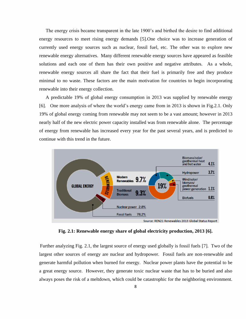
economic practicality. However, in the last five years the PV market has experienced rapid growth.
From 2010 to 2012 an additional 60 GW of new PV capacity was added globally, bringing the total
world capacity to 100 GW [6]. Fig.2.2 shows the exponential increase, especially over the last five
years of PV capacity.
Fig.2.2: Total World Capacity of PV (1995-2012) [6].
Page 23
10
The growth of installed PV can be recognized to many factors but the main reasons are
increases in environmental considerations, new state laws and regulations, purchase incentives,
increases in PV cell technology and efficiency, and decreases in overall system cost [7].
2.2 PHOTOVOLTAIC BACKGROUND
Solar panels are made up of photovoltaic cells; it means the direct conversion of sunlight to
electricity by using a semiconductor, usually made of silicon [9], [10]. The word photovoltaic
comes from the Greek meaning “light” (photo) and “electrical” (voltaic); the common abbreviation
for photovoltaic is PV [11]. Then PV efficiency increased continuously in the following years,
and costs have decreased significantly in recent decades. The main material used in the
construction of PV cells is still silicon, but other materials have been developed, either for their
potential for cost reduction or their potential for high efficiency [11]. Over the last 20 years the
world-wide demand for PV electric power systems has grown steadily. The need for low cost
electric power in isolated areas is the primary force driving the world-wide photovoltaic (PV)
industry today. PV technology is simply the least-cost option for a large number of applications,
such as stand-alone power systems for cottages and remote residences, remote telecommunication
sites for utilities and the military, water pumping for farmers, and emergency call boxes for
highways and college campuses [9]. PV cells are converting light energy, to another form of
energy, electricity. When light energy is reduced or stopped, as when the sun goes down in
the evening or when a cloud passes in front of the sun, then the conversion process stops or slows
down. When the sunlight returns, the conversion process immediately resumes, this conversion
without any moving parts, noise, pollution, radiation or constant maintenance. These advantages
are due to the special properties of semiconductor materials that make this conversion possible.
PV cells do not store electricity; they just convert light to electricity when sunlight is available. To
have electric power at night, a solar electric system needs some form of energy storage, usually
batteries, to draw upon [12].
2.3 PRINCIPLE OF PHOTOVOLTAIC SYSTEMS
Photovoltaic systems employ semiconductor cells, usually several square centimeters
in size [13]. Semiconductors have four electrons in the outer shell, on average.
Page 24
11
These electrons are called valence electrons [11]. When the sunlight hits the photovoltaic cells,
part of the energy is absorbed into the semiconductor. When that happens the energy loosens the
electrons which allow them to flow freely. The flows of these electrons are a current and when
you put metal on the top and bottom of the photovoltaic cells. We can draw that current to use it
externally, as shown in Fig. 2.3.
Fig.2.3: Principle of Photovoltaic cells.
Many cells are collected in a module to generate required power [13]. When many such cells
are connected in series and parallel combinations we get a solar PV module, the current rating of
the modules depends on the area of the individual cells. For obtaining higher power output the
solar PV modules are connected in series and parallel combinations forming solar PV arrays.
2.4 TYPES OF PV CELLS
Over the recent decades, silicon has been used for manufacturing more than 80% of solar cells
although other materials and techniques are developed. There are different types of solar cells
which differ in their material, price, and efficiency, since the efficiency is the percentage of solar
energy that is captured and converted into electricity. The efficiency values are an average
percentage of efficiency, because it's difficult to give an exact number for the different types of
solar panels output [10].
Page 25
12
Mono-crystalline Solar cells: They are made from a large crystal of silicon, see Fig.2.4. These
types of solar cells are the most efficient as in absorbing sunlight and converting it into
electricity. However they are the most expensive. They do somewhat better in lower light
conditions than the other types of solar cells. Also, their efficiency is around 15% - 18%.
Fig.2.4: Mono-crystalline Solar Panels
Polycrystalline Solar cells: This type of solar cell consists of multiple amounts of smaller
silicon crystals, see Fig.2.5.This type is instead of one large crystal have efficiency
approximately 15%.
Fig.2.5: Polycrystalline Solar Panels.
They are the most common type of solar panels on the market today. They look a lot like
shattered glass. They are slightly less efficient than the mono-crystalline solar cells and less
expensive to produce.
Amorphous Solar cells: This type is consisting of a thin-like film made from molten silicon
that is spread directly across large plates of stainless steel or similar material, see Fig.2.6. One
advantage of amorphous solar cells over the other two is that they are shadow protected.
Page 26
13
That means when a part of the solar panel cells are in a shadow the solar panel continues to
charge. These types of solar panels have lower efficiency than the other two types of solar panels,
and the cheapest to produce. These work great on boats and other types of transportation [10]. The
efficiency of this type is around 8 - 1 0 %.
Fig.2.6: Amorphous Solar Panels.
2.5 EQUIVALENT CIRCUIT AND MATHEMATICAL MODEL
There are different mathematical models that can be used to model a PV array. From the solid-
state physics point of view, the cell is basically a large area p-n diode with the junction positioned
close to the top surface [13], [14]. So a practical solar cell may be modeled by a current source in
parallel with a diode that mathematically describes the I-V characteristic.
Fig. 2.7: Equivalent Circuit of PV module.
Where Rs is the array series resistance, Rp is the array parallel resistance [14], [15]. Ns and Np
are the number of series and parallel modules respectively, I and V are the output current and
voltage of the array and Im is the module current and can be obtained from the following equation:
Page 27
14
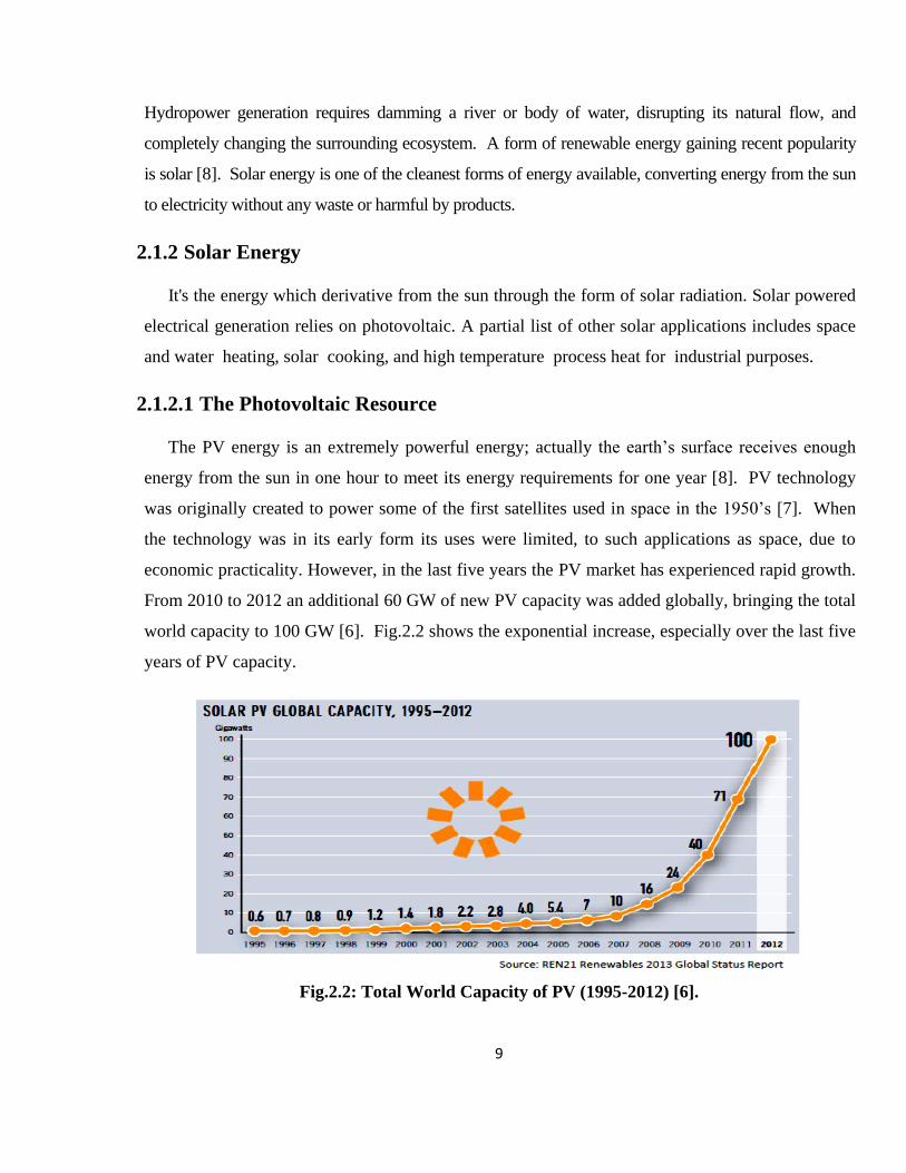
[ ( (
)
) ] (2.1)
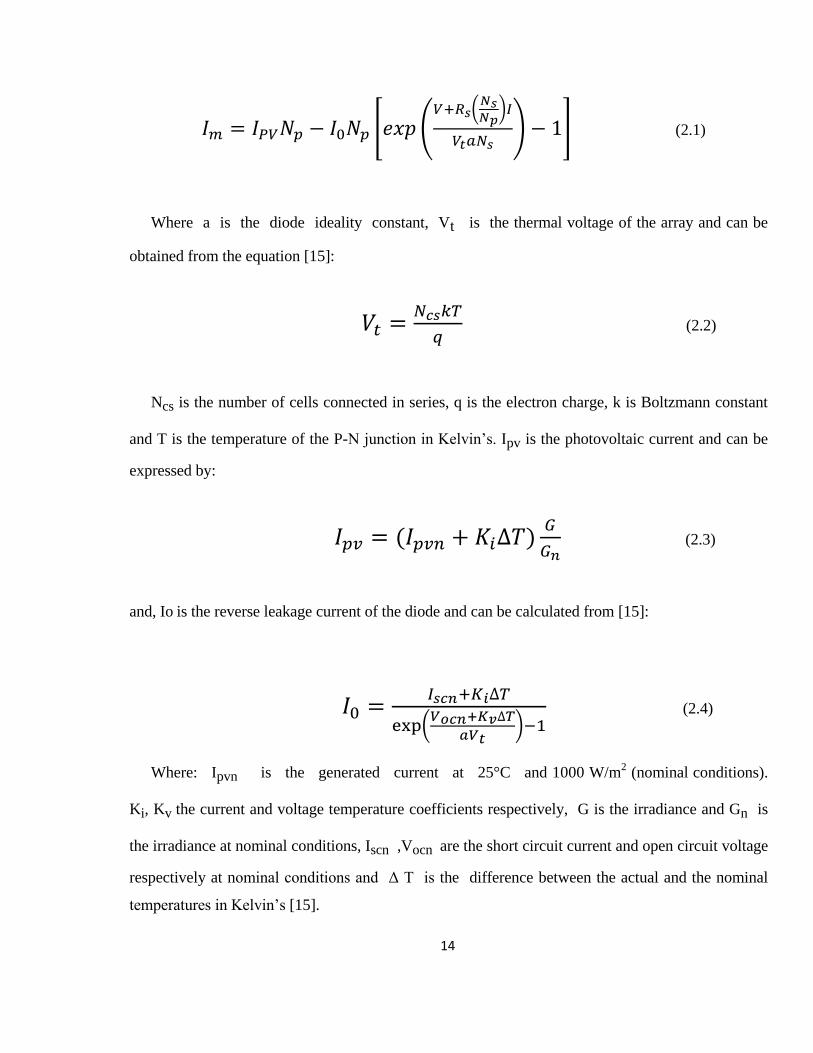
Where a is the diode ideality constant, Vt is the thermal voltage of the array and can be
obtained from the equation [15]:
(2.2)
Ncs is the number of cells connected in series, q is the electron charge, k is Boltzmann constant
and T is the temperature of the P-N junction in Kelvin‟s. Ipv is the photovoltaic current and can be
expressed by:
(2.3)
and, Io is the reverse leakage current of the diode and can be calculated from [15]:
(
)
(2.4)
Where: Ipvn is the generated current at 25°C and 1000 W/m2 (nominal conditions).
Ki, Kv the current and voltage temperature coefficients respectively, G is the irradiance and Gn is
the irradiance at nominal conditions, Iscn ,Vocn are the short circuit current and open circuit voltage
respectively at nominal conditions and Δ T is the difference between the actual and the nominal
temperatures in Kelvin‟s [15].
Page 28
15
2.6 NON LINEAR CHARACTERISTICS VERIFICATION
The parameters of the PV model used in this thesis are adjusted according to a real PV module
(Kyocera KC 200 GT) manufactured by Kyocera [16]. Fig.2.8 shows the I-V and P-V
characteristics of the PV module at different irradiances and constant temperature (25°C) and
Fig.2.9 shows the I-V and P-V characteristics of the PV module under constant irradiance and
different temperature.
Fig.2.8: I-V and P-V characteristics of the PV module at constant temperature 25°C and
various irradiances.
0 5 10 15 20 25 30 350
2
4
6
8
current (A
)
Voltage (V)
PV module : Kyocera KC200GT at constant temperature (25°C)
0 5 10 15 20 25 30 350
50
100
150
200
Pow
er (W
)
Voltage (V)
800W/m2
600W/m2
400W/m2
200W/m2
1000W/m2
1000 W/m2
800 W/m2
600 W/m2
400 W/m2
200 W/m2
Page 29
16
Fig.2.9: I-V and P-V characteristics of the PV module under constant irradiance and
different temperature.
Fig. 2.8 and Fig. 2.9 are obtained by simulation and the results are similar to that shown in the
PV module datasheet [16]. (See appendix A for the parameter and I-V curves of the PV module
datasheet).
Fig.2.10 shows The I-V and P-V characteristics of the PV array (Kyocera KC200GT; 8 series
modules; 63 parallel strings) at different irradiance (200,400,600,800,1000W/m2) and constant
temperatures (25°C).
0 5 10 15 20 25 30 350
5
10
curr
ent
(A)
Voltage (V)
PV module : Kyocera KC200GT at 1 kW/m2
0 5 10 15 20 25 30 350
100
200
Pow
er
(W)
Voltage (V)
75°C
50°C
25°C
75°C
50°C25°C
Page 30
17
Fig.2.10: I-V and P-V characteristics at constant temperature 25oC and various
irradiances for the PV array. (Kyocera KC200GT; 8 series modules; 63 parallel strings)
Photovoltaic's have nonlinear characteristics, where the performance and output power are
directly affected with the change of the operating conditions. It is clear from the previous figures
that the output power of PV's is directly proportional with the amount of solar irradiance falling on
it, and inversely proportional with its temperature. With the change of temperature and solar
irradiance the point at which maximum power point can be obtained also changes.
This means that the array terminal voltage must be varied using DC-DC converters in order to
track the maximum power point. Maximum power point tracking algorithms will be discussed in
details in chapter 3.
0 50 100 150 200 250 3000
200
400
600
curr
ent
(A)
Voltage (V)
PV Array : Kyocera KC200GT; 8 series modules; 63 parallel strings
0 50 100 150 200 250 3000
5
10
x 104
Pow
er
(W)
Voltage (V)
1000W/m2
800W/m2
1000W/m2
800W/m2
600W/m2
600W/m2
400W/m2
400W/m2
200W/m2
200W/m2
Page 31
18
2.7 PV APPLICATIONS
A photovoltaic application varies from solar farms that can generate hundreds of megawatts [9]
to small residential rooftop systems that only generate a few kilowatts. The ability for PV systems
to vary greatly in magnitude is a demonstration of how scalable and modular solar systems are
looking at every type of solar application, at the highest level each one can be lumped into one of
the two main types of PV system categories, either grid tied or off grid.
Fig.2.11: Typical grid - connected PV systems.
Off grid systems supply a local load and when the panel‟s generation exceeds the load the
excess energy is usually stored in a battery system for later use. Grid tied systems are connected to
the local utility network and can supply power back to the power grid when the panels generation
exceeds the local loads demand. Some grid connected systems still have battery storage capability.
For a residential system the local load is a home and everything inside consuming power. Both off
grid and grid tied systems can help offset a customer's net energy consumption, but grid tied
systems have the potential for the customer to sell back generated power at cost to the utility. Grid
connected PV systems represent around 90 % of the total PV installed power. Grid connected
distributed systems gained popularity in the last years, as they can be used as power generators for
grid connected customers or directly for the grid. Different sizes are possible since they can be
mounted on public or commercial buildings [17]. Grid connected systems produce and transform
the power directly to the utility grid. The configuration is usually ground mounted and the power
rating is above kW order [18].
Page 32
19
The typical configuration of a PV system can be observed in Fig.2.11. Depending on the
number of the modules, the PV array converts the solar irradiation into specific DC current and
voltage. A DC/DC boost converter is used when the voltage required by the inverter is too low and
to achieve the MPP. Energy storage devices can be included in order to store the energy produced
in case of grid support connection. The power conversion is realized by a three-phase inverter
which delivers the energy to the grid [19].
2.8 ADVANTAGES OF PV SYSTEMS
The advantages of photovoltaic [4] systems are:
PV systems are considered static electricity generators as they create electricity directly
from sunlight. They come prepackaged, ready to be mounted and wired. Modules contain
no moving parts, eliminating service and maintenance needs.
PV systems come in a range of sizes and output suitable for different applications. They
are lightweight, allowing for easy and safe transportation.
PV system can be easily expanded by adding more modules either in series to expand the
system's voltage or in parallel to enlarge the current.
PV systems are manufactured to withstand the most rugged conditions. Modules are
designed to endure extreme temperatures, at any elevation, in high winds, and with any
degree of moisture or salt in the atmosphere. Systems can be designed with storage
capabilities to provide consistent, high-quality power even when the sun isn't shining.
PV systems cause no noise or carbon emissions i.e. no pollution.
Page 33
20
The drawbacks of photovoltaic [4] systems are:
Very high manufacturing cost compared to other renewable resources.
Maximum power point problems.
Requires regular cleaning of its outer surfaces from dust.
Significantly low in efficiency.
2.9 SUMMARY
In this chapter, an overview of the importance of renewable energy, and photovoltaic
background and principle of photovoltaic systems are presented. The photovoltaic energy in
particular is reviewed with cell type, equivalent circuit, mathematical model and model
verification. The main PV system of a grid connected is also discussed and their advantages and
disadvantages are mentioned.
Page 34
21
CHAPTER 3
MPPT ALGORITHMS
Page 35
22
3.1 REVIEW OF MAXIMUM POWER POINT TRACKING
A set of photovoltaic cells called the solar panel. Photovoltaic cells are devices which detect
electromagnetic radiation and generate a current or voltage, or both, upon absorption of radiant
energy. The output power of PV arrays is mainly influenced by the irradiance (amount of solar
radiation) and temperature. Moreover for a certain irradiance and temperature, the output power
of the PV array is function of its terminal voltage and there is only one value for the PV's terminal
voltage at which the PV panel is utilized efficiently. The procedure of searching for this voltage is
called maximum power point tracking MPPT. Recently, several algorithms have been developed
to achieve MPPT technique such as; Perturb and Observe (P&O), incremental conductance, open
circuit voltage, short circuit current, fuzzy or neural based etc [20], [21],. However, the insulation
levels and the cell temperature determine only the limits of the best obtainable matching. The
array voltage determines the real matching. This mismatch can be improved by the use of a
MPPT controller to locate the local maximum power point in the p-v response range of the solar
panel [22], Fig.3.1 shows the P-V characteristics of a practical PV array showing MPP.
Fig.3.1: P-V characteristics of a practical PV array showing MPP.
0 50 100 150 200 2500
2
4
6
8
10
12x 10
4
Array Voltage (v)
Arr
ay P
ow
er
(Kw
)
Vmpp
Pmpp
Page 36
23
From the simulation results, the PV array under constant temperature 25oC and
irradiances 1000 W/m2 for PV array. The maximum readings appear to be 210.4V, 479A and 100.8
kW. The absolute maximum current (short circuit current) is 517A and the absolute maximum
voltage (open circuit voltage) is 263V.
3.2 MAXIMUM POWER POINT TRACKING
A PV panel has a nonlinear characteristics and its output power depends mainly on the
irradiance (amount of solar radiation) and the temperature. Moreover for the same temperature and
irradiance the output power of a PV panel is function of its terminal voltage. There is only one
value for the terminal voltage that corresponding to maximum output power for each particular
case. The procedure of searching for this voltage is called maximum power point tracking.
Maximum power point tracking of a PV panel can be obtained either in a single stage or in a double
stage. In the case of single stage, a DC/AC converter is utilized. On the other hand in case of
double stage a DC/DC and DC/AC converters are utilized. The characteristics of PV shown in
Fig.3.1 shows that the maximum power point for this particular panel lays at the values between
approximately 75-80% of array's open circuit voltage. Consequently, in this thesis the maximum
power point tracking algorithm scans the P-V curve at predefined voltage of 75% from the array‟s
open circuit voltage. The MPPT techniques are accomplished through the DC/DC converter which
interfacing the PV array to the inverter [23]. This can be achieved by controlling the input voltage
of the DC/DC converter. Fig.3.2 shows the Maximum power point tracker (MPPT) system as a
block diagram.
Fig.3.2: Maximum Power Point Tracker (MPPT) system as a block diagram.
Page 37
24
Maximum power point tracker (MPPT) tracks the new modified maximum power point in its
corresponding curve whenever temperature and/or insolation variation occurs. MPPT is used for
extracting the maximum power from the solar PV array and transferring that power to the grid. A
DC/DC (step up/step down) converter acts as an interface between the inverter and the array. The
MPPT changing the duty cycle to keep the transfer power from the solar PV array to the grid at
maximum point [22], [23].
The function of the inverter is to convert the output DC voltage of the PV into AC and to keep
the output voltage of the DC/DC converter constant. In order to accomplish that, two controllers are
required; one for the DC/DC converter, and the other for the inverter.
3.3 CONTROL ALGORITHMS
There are two algorithms which are used in this thesis for MPPT [24], [25]:
Hill Climbing methods
Fuzzy Based Algorithm
3.3.1 Hill Climbing Method
The hill climbing based techniques are so named because of the shape of the power-voltage
(P-V) curve. This technique is sub-categorized in two types:
Perturb & Observe Algorithm (P&O)
Incremental Conductance Algorithm (ICT)
3.3.1.1 Perturb and Observe method (P&O)
Perturb and Observe is a widely used method. It is common because of the simple feedback
structure and the fewer control perimeters. The basic idea is to give a trial increment or decrement
in the voltage, and if this result in an increase in the power, the subsequent perturbation is made in
the same direction or vice versa. This method is easy enough to handle and manipulate. However,
this method of monitoring the perimeter causes a delay and therefore tracking a real time maximum
power point is difficult [26-28].
Page 38
25
Usually voltage or duty ratio will be the parameter used to perturb the system. This algorithm is
not suitable when the variation in the solar irradiation is high. The voltage never actually reaches an
exact value but perturbs around the maximum power point (MPP) as in this method, after obtaining
the approximate maximum power point by scanning the entire P-V curve, the slope of the P-V
curve dP/dV is determined by giving the step change in duty ratio of boost converter. If due to
increase in duty cycle, the dP/dV decreases then next perturbation in duty cycle is kept unchanged
otherwise the sign of the perturbation step is changed [26]. Fig.3.3 shows the flow chart for
maximum power point tracking based Perturb and Observe algorithm.
Measure
V(k),I(k)
ΔVref(k) =Vref(k) - Vref(k-1)
ΔP(k) =P(k) - P(k-1)
ΔP(k) < 0
ΔVref(k) < 0
Yes
ΔVref(k) < 0
No
Reduce
Vref
Increase
Vref
YesNo
Reduce
Vref
Increase
Vref
Return
YesNo
Calculated Power
P(k)=V(k)*I(k)
P(k) = P(k-1)Yes
No
Fig.3.3: Flowchart for maximum power point tracking for (P&O) Algorithm.
Page 39
26
3.3.1.2 Incremental Conductance method (ICT)
The incremental conductance method [27-29] is based on the fact that the slope of the PV array
power curve is zero at the MPP, positive on the left of the MPP, and negative on the right, as given
by eq.(3.1).
, at MPP (3.1)
, left of MPP (3.2)
, right of MPP (3.3)
Since,
(3.4)
Using (3.4), the location of tracking point represented by equations (3.1, 3.2 & 3.3) is given by
eq. (3.5, 3.6, 3.7).
, at MPP (3.5)
, left of MPP (3.6)
, right of MPP (3.7)
The flow chart for maximum power point tracking for Incremental Conductance Algorithm is
shown in Fig.3.4.
Page 40
27
START
Sense : V(k) , I(k)
ΔV= V(k) - V(k-1)
ΔI= I(k) - I(k-1)
ΔV=0
ΔI=0ΔI/ΔV= - I/V
Yes
No
ΔI/ΔV > - I/V ΔI>0
No No
Increase VrefDecrease VrefDecrease VrefIncrease Vref
V(k-1)=V(k)
I(k-1)=I(k)
RETURN
No YesNoYes
YesYes
Fig.3.4: Flow Chart for maximum power point tracking for ICT Algorithm.
From eq. (3.8), the MPP can thus be tracked by comparing instantaneous conductance I/V to the
incremental conductance ΔI/ΔV as shown in the flow chart in Figure 3.4. The Incremental
Conductance Algorithm based tracking adjusts the duty cycle D of boost converter which adjusts
the operating voltage of PV array to operate at MPP. It is very unlikely for the ICT algorithm to
stop exactly on the MPP. Hence, practical ICT algorithm considers the MPP reached when the
operating point is within a certain error margin which is given by eq. (3.8):
(3.8)
This method gives a very good and accurate performance under rapidly varying conditions.
However, the drawback is that the actual algorithm is very complicated to handle. It requires
sensors to carry out the computations and high power loss through the sensors.
Page 41
28
3.3.2 Proposed Fuzzy Logic Controller Based Algorithm (FLC)
The maximum power point tracking speed is greatly reduced by performing the scanning in
larger steps and using the proposed fuzzy controller that gives faster convergence around the final
operating point [30], [31]. MPP fuzzy logic controller measures the values of the voltage and
current at the output of the solar cell, then calculates the power from the relation ( P=V*I ) to
extract the inputs of the controller. The crisp output of the controller represents the duty cycle of
the pulse width modulation to switch the DC/DC converter. The block diagram of the proposed
fuzzy logic controller (FLC) is shown in Fig.3.5.
Fig.3.5. Block diagram of Proposed Fuzzy (FLC) Based Tracking.
3.3.2.1 MPPT Fuzzy Logic Controller
The FLC examines the output PV power at each sample (time-k), and determines the change in
power relative to voltage (dp/dv). If this value is greater than zero the controller changes the duty
cycle for switching the boost converter to increase the voltage until the power is maximum or the
value (dp/dv) =0, if this value is less than zero the controller changes the duty cycle for switching
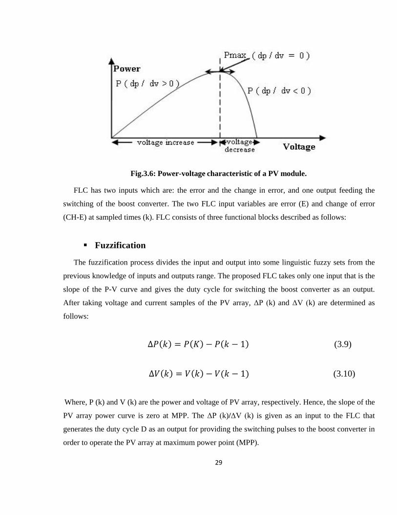
the boost converter to decrease the voltage until the power is maximum [32] as shown in Fig.3.6.
Page 42
29
Fig.3.6: Power-voltage characteristic of a PV module.
FLC has two inputs which are: the error and the change in error, and one output feeding the
switching of the boost converter. The two FLC input variables are error (E) and change of error
(CH-E) at sampled times (k). FLC consists of three functional blocks described as follows:
Fuzzification
The fuzzification process divides the input and output into some linguistic fuzzy sets from the
previous knowledge of inputs and outputs range. The proposed FLC takes only one input that is the
slope of the P-V curve and gives the duty cycle for switching the boost converter as an output.
After taking voltage and current samples of the PV array, ΔP (k) and ΔV (k) are determined as
follows:
(3.9)
(3.10)
Where, P (k) and V (k) are the power and voltage of PV array, respectively. Hence, the slope of the
PV array power curve is zero at MPP. The ΔP (k)/ΔV (k) is given as an input to the FLC that
generates the duty cycle D as an output for providing the switching pulses to the boost converter in
order to operate the PV array at maximum power point (MPP).
Page 43
30
The proposed FLC divides the input and output into seven linguistic fuzzy sets, Negative Big
(NB), Negative Medium (NM), Negative Small (NS), Zero (ZO), Positive Big (PB), Positive
Medium (PM) and Positive Small (PS). FLC has two inputs which are: error (E) and the change in
error (CH-E), and one output feeding to the DC-to-DC converter. The membership functions of the
input and output variables are shown in Fig. 3.7, Fig.3.8 and Fig.3.9 respectively.
Fig.3.7: Membership functions for input variable (E).
Fig.3.8: Membership functions for input variable (CH-E).
Fig.3.9: Membership functions for output variable (D).
Page 44
31
Fuzzy rule base
Based on the previous knowledge, the fuzzy rules should be precisely defined in order to
generate an output duty cycle as per the magnitude the slope of P-V curve to operate the PV array
at maximum power point. When the slope of P-V curve is positive then to reach towards MPP, the
duty ratio of boost converter is decreased in order to increase the PV operating voltage.
Similarly, if the slope of P-V curve is negative then to move the operating point at MPP, the
duty cycle is increased. The seven rules used for tracking the MPP in the proposed technique are
listed in Table 3.1.
E↓ /
CE→ NB NM NS ZE PS PM PB
NB ZE ZE ZE NB NB NB NB
NM ZE ZE ZE NM NM NM NM
NS NS ZE ZE NS NS NS NS
ZE NM NS ZE ZE ZE PS PM
PS PM PS PS PS ZE ZE PS
PM PM PM PM PM ZE ZE ZE
PB PB PB PB PB ZE ZE ZE
Table3.1. Fuzzy Rules.
Defuzzification
The deffuzification process generates the single crisp value of output duty cycle D from the
aggregated fuzzy set that includes a range of output values. The widely used centroid method [33],
[34] is used to convert the fuzzy subset of duty cycle D to real number. It computes the center of
gravity from the final output fuzzy set which is mathematically represented by,
∫
∫ (3.11)
Page 45
32
Where, Z* = D which is the output of fuzzy logic controller, ∫ denotes an algebraic integration
and Z is the aggregated fuzzy Set of output. Thus, the proposed fuzzy logic controller inherently
applies variable steps in duty ratio for controlling the boost converter as per the current operating
point and hence, gives faster convergence to maximum point.
3.4 DC-DC CONVERTERS
DC-DC converters have wide applications in PV systems. Whether it is boost converter [35],
[36], buck-boost converters or buck converters [37].
DC-DC converters are considered the main element in the maximum power point tracking
process and without it the maximum power could not be achieved. In this thesis, the boost
converter is used to change the terminal voltage of the PV array and from which maximum power
point tracking can be obtained.
3.4.1 Boost Converters
The maximum power point tracking is essentially a load matching problem. A DC - DC
converter is required for changing the input resistance of the panel to match the load resistance by
varying the duty cycle. (See appendix B for details on boost converter's theory of operation). Since
this thesis work deals with the boost converter, further discussions will be focused on this one [35],
[36].The Boost converter circuit diagram is shown in Fig.3.10.
Fig.3.10: Boost Converter Circuit Diagram.
The relation between the output voltages over the input voltage is:
(3.12)
Page 46
33
Where, Vs is the input voltage to the boost converter Vo is the output voltage, and D is the duty
cycle. In this thesis, Vo is fixed using the voltage -sourced converter (VSC), and Vs is at the same
time the array terminal voltage which is controlled by varying the duty cycle D.
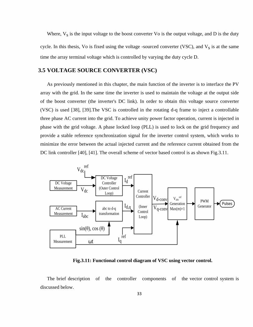
3.5 VOLTAGE SOURCE CONVERTER (VSC)
As previously mentioned in this chapter, the main function of the inverter is to interface the PV
array with the grid. In the same time the inverter is used to maintain the voltage at the output side
of the boost converter (the inverter's DC link). In order to obtain this voltage source converter
(VSC) is used [38], [39].The VSC is controlled in the rotating d-q frame to inject a controllable
three phase AC current into the grid. To achieve unity power factor operation, current is injected in
phase with the grid voltage. A phase locked loop (PLL) is used to lock on the grid frequency and
provide a stable reference synchronization signal for the inverter control system, which works to
minimize the error between the actual injected current and the reference current obtained from the
DC link controller [40], [41]. The overall scheme of vector based control is as shown Fig.3.11.
DC Voltage
Measurement
AC Current
Measurement
PLL
Measurement
DC Voltage
Controller
(Outer Control
Loop)Vdc
abc to d-q
transformationIabc
sin(θ), cos (θ)
Current
Controller
(Inner
Control
Loop)
Vdcref
Iqref
Idref
Id,q
Vabcref
Generation
Max(m)=1
Vd-conv
Vq-conv
PWM
GeneratorPulses
ωt
Fig.3.11: Functional control diagram of VSC using vector control.
The brief description of the controller components of the vector control system is
discussed below.
Page 47
34
3.5.1 DQ Transformation
DQ transformation is the transformation of coordinates from the three-phase stationary
coordinate system to the d-q rotating coordinate system. This transformation is made in two Steps:
A transformation from the three-phase stationary coordinate system to the two-phase, α-β
stationary coordinate system and
A transformation from the α-β stationary coordinate system to the d-q rotating coordinate
system.
Clark and Inverse-Clark transformations are used to convert the variables (e.g. phase values of
voltages and currents) into stationary α-β reference frame and vice-versa. Similarly, Park and
Inverse-Park transformations convert the values from stationary α-β reference frame to
synchronously rotating d-q reference frame, and vice versa. The reference frames and
transformations are shown in Fig.3.12.
Fig.3.12: Transformation of axes for vector control.
The stationary α-axis is chosen to be aligned with stationary three phase a-axis for simplified
analysis. The d-q reference frame is rotating at synchronous speed ω with respect to the stationary
frame α-β, and at any instant, the position of d-axis with respect to α-axis is given by θ=ωt. The
summary of the transformation is presented in tabular form in Appendix-C.
Page 48
35
3.5.2 Phase Locked Loop (PLL)
The phase-locked loop technique [42] has been used as a common way to synthesize the phase
and frequency information of the electrical system, especially when it‟s interfaced with power
electronic devices. The Phase Locked Loop block [43] measures the system frequency and provides
the phase synchronous angle θ (more precisely [sin (θ), cos (θ)]) for the d-q Transformations block.
In steady state, sin (θ) is in phase with the fundamental (positive sequence) of the α component and
phase A of the PCC voltage Vabc. In the three-phase system, the d-q transform of the three-phase
variables has the same characteristics and the PLL system can be implemented using the d-q
transform. The block diagram of PLL system can be described in Fig.3.13.
Fig.3.13: Schematic diagram of the phase locked loop (PLL).
3.5.3 Vector Control
For analysis of the voltage source converter using vector control, three phase currents and
voltages are described as vectors in a complex reference frame, called α-β frame. A rotating
reference frame synchronized with the AC-grid is also introduced, as in Figure.3.12. As the d-q
frame, is synchronized to the grid, the voltages and currents occur as constant vectors in the d-q
reference frame in steady state. For the analysis of the system, basic equations describing the
system behavior are presented based on analysis done in [38], [39]. Considering the converter
system connected to grid, and defining grid voltages as Vabc , currents Iabc , and converter voltages
Vconv , and resistance (R) and inductance (L) between the converter and the grid. The voltage of the
converter can be expressed as:
(3.13)
Page 49
36
Using the a-b-c to d-q transformations, the converter 3-phase currents and voltages are
expressed in 2-axis d-q reference frame, synchronously rotating at given AC frequency ω.
[
] [
]
[ ] [
ω
ω ] [
] [
] (3.14)
The voltage equations in d-q synchronous reference frame are,
ω (3.15)
ω (3.16)
The system equations of Eqn. (3.15, 3.16) are rewritten as follows,
ω (3.17)
ω (3.18)
3.5.3.1 DC-Voltage Controller
The dc voltage controller is discussed as the outer controller. Dimensioning of the dc link
voltage controller is determined by the function between the current reference value to be given and
the dc link voltage. The general Simulink model of the external controller can thus be given as in
Fig.3.14. For the PI controller block of the function of K(s) the outer voltage control can be
implemented based on Equation (3.19).
( ) [
] (3.19)
Page 50
37
Fig.3.14: Simulink Model of the DC-Voltage Controller.
3.5.3.2 Inner Current Controller
The inner current control loop can be implemented in the d-q-frame, based on the basic
relationship of the system model equations (3.17, 3.18). Inside the current controller as shown in
Fig.3.15, the PI regulator for d and q axis current control which transform the error between the
comparison of d and q components of current into voltage value.
1
Vdc_ref
Vdc_ref
+-
2Vdc_mes
PI +-
Id_ref
3Id_mes
PI ++
Vd’
CCPCross-Coupling
Part
Vd’’
-+
4Vd_meas
5 +-
6Iq_mes
PI ++
Vq’
CCP
Cross-Coupling
Part
Vq’’
-+
7Vq_meas
Iq_ref
Iq_ref
Vd_Conv
Vq_Conv
Sum
dq2abc 8
Vabc
V_abc
DC_Voltage Regulator Current Regulator
Fig.3.15: Total converter control scheme.
Page 51
38
It‟s shown in Fig.3.15 that the control signal is the output of the PI regulator K(s) that
processes the error signals Id-ref - Id. Similarly, is the output of the PI regulator K(s) that
processes the error signals Iq-ref - Iq. In order to generate the converter voltage signals ,
the PWM modulation pulses are produced by transformation the converter signals to pulses. The
pulses for voltage source inverter are fired by using sine-triangular modulation.
3.6 SINUSOIDAL PULSE WIDTH MODULATION (SPWM)
The DC-AC inverters usually operate on Pulse Width Modulation (PWM) technique. The
PWM is a very useful technique in which width of the gate pulses are controlled by various
mechanisms. PWM inverter is used to keep the output voltage of the inverter at the rated
voltage irrespective of the output load. The pulse width modulation inverter has been the
main choice in power electronic for decades, because of its circuit simplicity and strong control
scheme [44]. Depending on the switching performance and good characteristic features, Sinusoidal
Pulse Width Modulation (SPWM) will be used and the modulating signal as illustrated in Fig.3.16.
As mentioned in [45], the advantages of using SPWM include low power consumption, high energy
efficient up to 90%, high power handling capability, no temperature variation-and aging-
caused drifting or degradation in linearity and SPWM is easy to implement and control.
SPWM techniques are characterized by constant amplitude pulses with different duty cycle
for each period [46] .(see Appendix D for details on Sinusoidal Pulse Width Modulation (SPWM)
theory of operation).
Fig.3.16: Pulse width modulation waveforms.
Page 52
39
3.7 SUMMARY
In this chapter, the maximum power point tracking problem is discussed, and the boost type of
DC-DC converters, which is the main tool used for obtaining the maximum power point are
mentioned. The operation of the boost converter is also discussed. Further on, different famous
MPPT algorithms are mentioned and their advantages and disadvantages are also highlighted, and
then the three main algorithms used in this thesis (P&O, ICT and FLC) are discussed in more
details along with the control scheme of the DC-AC inverter.
Page 53
40
CHAPTER 4
POWER QUALITY TERMS
AND DEFINITIONS
Page 54
41
4.1 INTRODUCTION
With the dramatic increases over the last 20 years in energy conversion systems utilizing power
electronic devices, we have seen the emergence of "power quality" as a major field of power
engineering. Simply, power electronic technology has played a major role in creating “power
quality” and simple control algorithm modifications to this same technology can often play an
equally dominant role in enhancing overall quality of electrical energy available to end-users.
4.2 DEFINITION OF POWER QUALITY
"Power quality is a set of electrical boundaries that allows a piece of equipment to function in its
intended manner without significant loss of performance or life expectancy" This definition
embraces two things that we demand from an electrical device: performance and life expectancy.
Any power-related problem that compromises either attribute is a power quality concern. Many
sources in the literature have addressed the importance of power quality; however, there is no
single agree definition for the term “power quality”, and various sources have different and
sometimes inconsistent definitions for it. In addition, “power quality” is sometimes used loosely to
express different meanings: “supply reliability”, “service quality”, “voltage quality”, and “current
quality” [47]. The multiple meanings of power quality are the result of defining power quality from
different perspectives. Power quality, in generation, relates to the ability to generate electric power
at a specific frequency, 50 or 60 Hz, with very little variation; while power quality in transmission
can be referred to as the voltage quality. At the distribution level, power quality can be a
combination of voltage quality and current quality. From the marketing point of view, electricity is
a product and the power quality is the index of the product quality [48].
Several engineering organizations and standard bearers in several parts of the world are
spending a large amount of resources to generate power quality standards. Following some of
power quality definition and related standards. The Institute of Electrical and Electronics Engineers
(IEEE) defines power quality in the IEEE standard 1159-1995 as: “power quality is the concept of
powering and grounding sensitive equipment in a matter that is suitable to the operation of that
equipment” [49]. This definition limits the term power quality to only sensitive equipment, and this
definition narrows down the impact of harmonic currents to consider it as affecting only that
equipment [49].
Page 55
42
It is hard to distinguish between voltage disturbances and current disturbances due to the close
relationship between the two, and there is no common reference point that the disturbance can be
seen from. For instance, starting a large induction motor leads to an over current; this is a current
disturbance from the network perspective. However, the neighboring loads can suffer from a
voltage dip, which is considered a voltage disturbance from another perspective. This action,
starting an induction motor, leads to a disturbance that can be looked at from different perspectives:
as a voltage disturbance from one point and a current disturbance from the other. The
distinguishing complexity makes using the term “power quality disturbance” more preferable in
general [50]. Much recent research has focused on classifying power quality disturbances according
to the underlying causes [51], but it is still a difficult classification. However, the typical power
quality disturbance classification is usually based on voltage magnitude and frequency variation for
different time durations.
4.3 POWER QUALITY DISTURBANCES CLASSIFICATION
The effects of power disturbances vary from one piece of equipment to another and with the age
of the equipment. Equipment that is old and has been subjected to harmful disturbances over a
prolonged period is more susceptible to failure than new equipment. With the purpose of classify
different types of power quality disturbances, the characteristics of each type must be known. In
general, power quality disturbances are classified into two types: steady state and non-steady state.
This classification is done in terms of the frequency components which appear in the voltage
signals during the disturbance, the duration of the disturbance, and the typical voltage magnitude.
These disturbances are mainly caused by [52]:
External factors to the power system: for example, lightning strikes cause impulsive
transients of large magnitude.
Switching actions in the system: a typical example is capacitor switching, which causes
oscillatory transients.
Faults which can be caused, for example, by lightning (on overhead lines) or
insulation failure (in cables). Voltage dips and interruptions are disturbances related to
faults.
Loads which use power electronics and introduce harmonics to the network.
Page 56
43
Different power quality disturbances will be discussed below:
4.3.1 Transients
Transients are sudden but significant deviations from normal voltage or current levels. On the
subject of describing a phenomenon or a quantity that varies between two consecutive steady states
during a time interval that is short compared to the time scale of interest.
A transient can be a unidirectional impulse of either polarity or a damped oscillatory wave with
the first peak occurring in either polarity [49]. Transients refer to variations in the voltage
waveform, which results in over-voltage conditions for a fraction of a cycle of the fundamental
frequency. Transients are classified as impulsive or oscillatory.
4.3.2 Short-Duration Variations
These are variations of the RMS (root mean square) value of the voltage from nominal voltage
for a time greater than 0.5 cycles of the power frequency but less than or equal to 1 minute. Usually
further described using a modifier indicating the magnitude of a voltage variation (e.g., sag, swell,
or interruption), and possibly a modifier indicating the duration of the variation (e.g.,
instantaneous, momentary, or temporary) [49]. Table 4.1 shows the different characteristics of
short-duration voltage variations.
4.3.2.1 Voltage Sag (Dip)
One of the most common power frequency disturbances is voltage sag. By definition, voltage
sag is an event that can last from half of a cycle to several seconds. Common causes of voltage sags
are short circuits (faults) on the electric power system, motor starting, customer load additions, and
large load additions in the utility service area. Voltage sags well-defined as decrease to between 0.1
and 0.9 pu in RMS voltage or current at the power frequency for durations of 0.5 cycles to 1
minute.
Page 57
44
4.3.2.2 Voltage Swell
A voltage swell is a short duration increase in voltage values. Voltage swells lasting longer than
two minutes are classified as over voltages. Voltage swells are commonly caused by large load
changes and power line switching. If swells reach too high a peak, they can damage electrical
equipment. The utility's voltage regulating equipment may not react quickly enough to prevent all
swells or sags. Voltage swells well-defined as increase in RMS voltage or current at the power
frequency for durations from 0.5 cycles to 1 minute. Typical values are 1.1 – 1.8 pu.
4.3.2.3 Voltage Interruption
This is complete loss of voltage (< 0.1 pu) on one or more phase conductors for a time period
between 0.5 cycles and 3 seconds (momentary), and between 3 seconds and 1 minute
(temporary).
4.3.3 Long-Duration Variations
This is a variation of the RMS value of the voltage from nominal voltage for a time greater
than 1 minute, usually further described using a modifier indicating the magnitude of a voltage
variation (e.g., under-voltage, over-voltage, or voltage interruption). It is caused by load
variations on the system or system switching operations.
4.3.3.1 Over-voltage
This is a measured voltage having a value greater than the nominal voltage for a period of time
greater than 1 minute. Typical values are 1.1 – 1.2 pu.
4.3.3.2 Under-voltage
This is a measured voltage having a value less than the nominal voltage for a period of time
greater than 1 minute. Typical values are 0.8 – 0.9 pu.
Page 58
45
The general characteristics of over-voltage, under-voltage, and sustained interruptions are
summarized in Table 4.1 as indicated in [49].
Table 4.1: Characteristics of Short-Duration Variations and typical causes.
Short-Duration Variations Typical Spectral
Content
Typical Duration Typical Voltage
Magnitude
A. Instantaneous
Sag ----- 0.5 – 30 cycles 0.1 – 0.9 pu
Swell ----- 0.5 – 30 cycles 1.1 – 1.8 pu
B. Momentary
Interruption ----- 0.5 – 3 sec. < 0.1 pu
Sag ----- 30 cycles – 3 sec. 0.1 – 0.9 pu
Swell ----- 30 cycles – 3 sec. 1.1 – 1.4 pu
C. Temporary
Interruption ----- 3 sec. – 1 min. < 0.1 pu
Sag ----- 3 sec. – 1 min. 0.1 – 0.9 pu
Swell ----- 3 sec. – 1 min. 1.1 – 1.2 pu
Typical Sag causes Remote system faults, large loads, and non-linear loads
Typical Swell causes Remote system faults, large loads, and non-linear loads
Typical Interruption causes System protection and maintenance
4.3.4 Harmonics
Harmonics are sinusoidal voltages or currents having frequencies that are integer multiples of
the frequency at which the supply system is designed to operate. Harmonics in conjunction with
the fundamental voltage or current can produce waveform distortion. Harmonic distortion exists
due to nonlinear characteristics of devices and loads on the power system. Voltage distortion
results as these currents cause nonlinear voltage drops across the system impedance.
Harmonic distortion is a growing concern for many customers and for the overall power system
due to increasing application of power electronics equipment.
Page 59
46
Harmonic distortion levels can be found throughout the complete harmonic spectrum.
Furthermore, the phase angle of each component is unique. It is also common to use a single
quantity, the total harmonic distortion (THD), as a measure of the magnitude of harmonic
distortion.
Each classification category has its own technical features, which can be considered the key to
detecting and identifying the different types of disturbances in electrical systems. For instance,
voltage sags or voltage swells can be detected by noticing the variation in the voltage magnitude for
a specific duration.
4.4 SIGNAL ANALYSIS
This is the step for monitoring power quality disturbances. It involves signal processing
techniques in order to analyze the detected disturbance signals. The main objective of the
analysis procedure is to justify the disturbance signal‟s features. These features can lead to the
identification of the type of disturbance that occurred, and the more features justified from the
signal analysis the more accurate disturbance identification. There are many signal processing
techniques that have been used to analyze the disturbance signals; a quick review of some
techniques is presented below.
Fast Fourier Transform (FFT)
FFT is a basic method used widely in signal processing. FFT is applied to extensive data that
has been selected based on various measurements. The FFT spectrum is normally used for
detecting dominant harmonics, inter-harmonics and their related magnitudes.
Short-Time Fourier Transform (STFT)
STFT provides time-frequency signal decomposition, which is equivalent to applying a set of
equal-bandwidth sub-band filters. STFT is a Fourier-related transform used to determine the
sinusoidal frequency and phase content of local sections of a signal as it changes over time.
Page 60
47
Continuous STFT and discrete STFT are examples of short-Time Fourier Transform. There are
other kinds of transforms and filters that have been applied to power quality problems; however,
research on power quality problem analysis is still developing. After data have been analyzed, these
data are characterized into specific classes to extract information about the type of power quality
disturbance.
4.5 CONCLUSION
Utilities in deregulated systems can no longer deal with power quality problems as a single
entity. Thus, identifying who is responsible for any power quality problem will be a very
important task in mitigating that problem. Moreover, the increase in nonlinear loads, which are
sources of harmonic currents, makes the identification too complex. In light of this definition of
power quality, this chapter provides an introduction to the more common power quality terms.
Along with definitions of the terms, explanations are included where necessary. This chapter also
attempts to explain how power quality factors interact in an electrical system.
Page 61
48
CHAPTER 5
SIMULAION RESULTS
Page 62
49
5.1 INTRODUCTION
This chapter shows all the simulation of the photovoltaic array, the boost converter, the proposed
fuzzy logical control (FLC), Perturb and Observe (P&O), and Incremental Conductance (ICT)
algorithms. Also, in this thesis the grid disturbances effects on a grid connected PV array were
studied while considering different maximum power point tracking algorithms. The grid disturbances
involved are the different types of faults, voltage sag, and voltage swell. A comparative study of the
grid disturbances effect on the three maximum power point tracking algorithms is discussed. All the
simulation results are done using MATLAB/SIMULINK software.
5.2 SYSTEM UNDER STUDY
The complete system is to be simulated using the MATLAB/SIMULINK (as shown in Fig.5.1),
and by varying the operating condition (solar irradiance and temperature), for the three different
control algorithms, P&O algorithm, ICT algorithm and FLC proposed algorithm. The PV array is
composed of (63 * 8) parallel and series modules respectively with a total output power of 100 kW.
PVArray
DC/ACInverter
DC/DCBOOST
Converter
Controller
IV
PWMSPWM
Utility Grid
Fig.5.1: Block diagram of the grid connected photovoltaic system.
Page 63
50
Table 5.1, shows the simulation parameters for the proposed system
Table 5.1: SIMULATION PRAMETERS
Quantity Value
Grid voltage 260V
Frequency 60 Hz
Switching frequency 5kHz
DC link capacitor C 100µF
DC link Voltage 500V
Converter inductance 5mH
Converter Capacitor 1.2mF
Sampling period 1µS
5.3 PV MODELING FOR SIMULATION
The mathematical model used for this simulation is shown in equation (5.1)
(
)
(5.1)
The various components used in developing the circuit design for a PV module are chosen from
the MATLAB/SIMULINK library. The voltage measurement block, current measurement block,
go to block, from block, and control current source block are used to model various outputs such as
Shockley diode current, the light generated photovoltaic current, cell temperature equation, and
power output.
Fig.5.2 shows the Simulink modeling for the reverse saturation current ( ) at the reference
temperature which is given by the equation (5.1).
Page 64
51
Fig.5.2: Simulink Model for Evaluating
Fig.5.3 shows the Simulink model for the light generated current of the photovoltaic cell which
is a linear function of temperature and solar radiation as shown in the equation (5.2) below:
(5.2)
Fig.5.3: Simulink Model for Evaluating
Fig.5.4 shows the Simulink model to evaluate the model current referring to the appropriate
model circuit for which is given by the equation (5.3).
[ ( (
)
) ] (5.3)
Page 65
52
Fig.5.4: Mathematical Model Implementation for Model Current
The MATLAB/SIMULINK model of the simulated PV is shown in Fig.5.5
Fig.5.5: Simulation of the Photovoltaic Module.
The current is passed through series and parallel resistors of the array as shown in Fig.5.5,
and then all these blocks are converted to one sub system block with two inputs (Temperature, and
Irradiation) as shown in Fig.5.6.
Page 66
53
Fig.5.6: PV model Subsystem.
The MATLAB/SIMULINK model is tested by inserting all the required data shown in Table 5.2
to simulate the KYOCERA KC200 GT module. The data sheet [16] of the simulated module is
shown in appendix A.
Table 5.2: KC200GT module parameters
Quantity Value
I max power 7.61 A
V max power 26.3 V
P max 200.143 W
I short circuit 8.21 A
V open circuit 32.9 V
I leakage 9.825*10-8
A
I photovoltaic 8.211 A
Diode ideality constant (a) 1.3
Parallel resistance 415.406 Ω
Series resistance 0.221 Ω
5.4 BOOST CONVERTER MODEL
As the name implies, the boost or step-up converter has an output voltage that is always greater
than the input voltage. The boost converter also has the added advantage that the output can be
isolated from the input.
Page 67
54
The MATLAB/SIMULINK model of boost converter model is shown in Fig.5.7. The boost
converter plays a very important role as it varies the PV array terminal voltage with the change of
the duty cycle. The duty cycle will be determined depending on the signal of the maximum power
point tracker whether it is P&O, ICT or FLC as it discussed in the following sections.
Fig.5.7: Block Diagram of Boost Converter Model.
5.5 PERTURB AND OBSERVE CONTROLLER
The perturb and observe algorithm discussed in chapter 3 is constructed using MATLAB M-
FILE code within SIMULINK, the code is shown in appendix E and its output is connected to the
boost converter to achieve the maximum power point tracking. Fig.5.8 shows the SIMULINK
model of the MPPT using P&O method.
Fig.5.8: Maximum Power Point Controller Using P&O.
Page 68
55
5.6 INCREMENTAL CONDUCTANCE CONTROLLER
The incremental conductance algorithm discussed in chapter 3 (section 3.4.1.2) is constructed
using MATLAB/ SIMULINK TOOLBOX, and its output is connected to the boost converter to
achieve the maximum power point tracking. Fig.5.9 shows the SIMULINK model of the MPPT
using ICT method.
Fig.5.9: Maximum Power Point Controller Using ICT.
5.7 PROPOSED FUZZY LOGIC CONTROLLER
The designed fuzzy logic controller is connected between PV module and DC-to-DC
converter module to track the MPP, as shown in Fig.5.10 which illustrates the sub-system using
MATLAB/ SIMULINK, and its output is connected to the boost converter to achieve the maximum
power point tracking.
Fig.5.10: Controlling the PV power using FLC.
Page 69
56
The purpose of learning mechanism is to learn the environmental parameters and to modify the
fuzzy logic controller accordingly so that the response of the overall system is close to optimum
operation point. The learning mechanism is composed of inverse fuzzy model and knowledge base
modifier:
Inverse fuzzy model
In this part, we use error (E) and change of error (CH-E) of system and control the knowledge
base modifier to modify fuzzy parameter to optimize the operation of system. The fuzzy parameter
can be adapted by this condition If error < ε (limit value) then knowledge base modifier will be done.
Knowledge base modifier
In this part fuzzy parameter will be modifier as follow:
a) Scaling factor
Quite simple schemes for altering the scaling factor to meet various performance criteria can be
devised. The range of the error, change of error and also output of fuzzy can be set like balance
between proportional and integral control.
b) Fuzzy set membership function
In this part, tuning peak values, such as error, can improve both responsiveness and stability.
The large error can improve responsiveness and small error can improve stability. The modification
is performed by shifting the membership functions of both input and output.
Also we can show the three directions of the two inputs and output membership function as
shown in Fig.5.11.
Page 70
57
Fig.5.11: Fuzzy logic membership functions after tuning in three directions.
c) Tuning rule base
Modifying rule base can affect the control system such as overshoot, settling time, stability,
responsiveness. Rule base and fuzzy set membership function have relationship with each other
depending on the quantity of error and change of error like in Table 3.1.
5.8 INVERTER CONTROLLER
Voltage Source Converter Controller (VSC) is performed on the three phase inverter to keep
the DC- link voltage constant at any required value. The whole process discussed before in chapter
3 (sections 3.6) is simulated on SIMULINK, as shown in Fig.5.12
Fig.5.12: Control of three phase inverter.
Page 71
58
The inverter succeeded to keep the DC link voltage at a constant value which makes the DC-DC
converter's task of MPPT mush easier. At the same time the inverter converts the DC power into
AC and that is its main task so that the PV system could be easily connected with the grid.
Fig.5.13: DC-link voltage VS Reference voltage.
5.9 SIMULATION RESULTS
All the discussed features in this chapter are to be bound together to form a complete grid-
connected PV system as seen in Fig.5.14. The system shown in Fig.5.1 is modeled and simulated
utilizing the Sim Power System toolbox under the MATLAB/Simulink. The MATLAB model is
shown in Fig.5.14. This model is simulated under three conditions; First, by utilizing the Perturb &
Observe (P&O) technique, second, by utilizing the Incremental Conductance technique, and finally
by utilizing the Fuzzy logic based algorithm.
Fig.5.14: The MATLAB/ Simulink model of the system under investigation.
0.05 0.1 0.15 0.20
500
1000
Time(S)
DC
Voltage
Ref-DC Voltage
DC-Link Voltage
Page 72
59
5.9.1 STEADY STATE ANALYSIS
The investigated system consists of a 100 kW PV array which is connected to a boost converter,
and then the boost converter is connected to the grid via a three phase inverter. The PV panel
utilized in this thesis is KYOCERA KC200GT. The MATLAB model of the PV Panel was
described and verified in chapter 2 (section 2.5 and 2.6). In this study, the 100 kW array consists of
63 parallel string each comprise 8 series connected panel. The parameters of the investigated
system are given in Table 5.1.
First the simulation is obtained while applying the P&O algorithm and set the irradiances to
1000 W/m2 and the temperature to 25
oC. Fig.5.15 shows the output voltage, current, and power of
the PV array terminal.
Fig.5.15. Voltage, Current and Power Output of PV array with MPPT Based P&O.
0 0.5 1 1.5 20
200
400
Voltage (
V)
Time (S)
PV Array : Kyocera KC200GT of 8 series modules; 63 parallel strings
0 0.5 1 1.5 20
500
1000
Curr
ent
(A)
Time (S)
0 0.5 1 1.5 20
100
200
Pow
er
(kW
)
Time (S)
Page 73
60
Then the simulation is achieved while applying the incremental conductance technique under the
same condition. Fig.5.16 shows the output voltage, current, and power of the PV array terminal.
Fig.5.16: Voltage, Current and Power Output of PV array with MPPT Based ICT.
Finally, the simulation is accomplished under the same condition while applying the fuzzy logic
based algorithm. Fig.5.17 shows the output voltage, current, and power of the PV array terminal.
It can be observed that PV array feeds 100 kW to the grid while utilizing the three algorithms
but the proposed FLC is accurate and give a high response when compared with the others as
shown in Fig.5.17 which illustrates the performance of the proposed FLC.
0 0.5 1 1.5 20
200
400
Voltage (
V)
Time (S)
PV Array : Kyocera KC200GT of 8 series modules; 63 parallel strings
0 0.5 1 1.5 20
500
1000
Curr
ent
(A)
Time (S)
0 0.5 1 1.5 20
100
200
Pow
er
(kW
)
Time (S)
Page 74
61
Fig.5.17: Voltage, Current and Power Output of PV array with MPPT Based FLC.
The array output power for the three techniques under constant irradiance (1000 W/m2) is
shown in Fig.5.18.
Fig.5.18: The output power of the PV array using the three different algorithms
at constant irradiance.
0 0.5 1 1.5 20
200
400
Voltage (
V)
Time (S)
PV Array : Kyocera KC200GT of 8 series modules; 63 parallel strings
0 0.5 1 1.5 20
500
1000
Curr
ent
(A)
Time (S)
0 0.5 1 1.5 20
100
200
Pow
er
(kW
)
Time (S)
0 0.5 1 1.5 20
50
100
150
Pow
er
(kW
)
Time (S)
PV Array : Kyocera KC200GT of 8 series modules; 63 parallel strings
P&O
ICT
FLC
Page 75
62
The performance of rise time, settling time, and peak time of three different algorithms are
summarized in Table 5.3, which show that the Fuzzy-controller is a best control system.
Table 5.3: The performance of three different algorithms
Type of Algorithm
The response of three different algorithms
Rise Time
(sec)
Settling Time
(sec)
Peak Time
(sec)
With P&O controller 0.0510 0.0885 0.2360
With ICT controller 0.0377 0.0674 0.1834
With FLC controller 0.0032 0.0232 0.1525
The three techniques are compared by changing the irradiance from 1000 W/m2 to 250W/m
2
then to 1000W/m2 then to 250W/m
2 and then finally to 1000 again as seen in Fig.5.19.
Fig.5.19: The output power of the PV array using the three different algorithms
at variable irradiance.
It can be seen that the fuzzy based algorithm shows faster response in tracking the maximum
power point under variable and constant irradiance and gives minimum oscillations around the final
operating point compared to ICT and P&O based algorithm. It can be also seen from Fig.5.18, and
Figure 5.19, that the P&O algorithm gives slower response, whereas the ICT algorithm gives
relatively lower response as compared to the fuzzy based algorithm. Therefore the FLC gives
relatively less oscillation and the highest response as compared to the P&O and ICT.
0 0.5 1 1.5 20
50
100
150
Po
we
r (k
W)
Time (S)
PV Array : Kyocera KC200GT of 8 series modules; 63 parallel strings
P&O
ICT
FLC
Page 76
63
5.9.2 TRANSIENT ANALYSIS
In order to be able to categorize different types of power quality disturbances, the characteristics
of each type must be known. In general, power quality disturbances are classified in terms of the
frequency components which appear in the voltage signals during the disturbance, the
duration of the disturbance, and the typical voltage magnitude. The power quality disturbances are
classified in chapter 4.
5.9.2.1 FAULT ANALYSIS
In this section the MATLAB/SIMULINK model shown in Fig.5.20 is simulated under different
fault conditions [53]. The simulation is accomplished under nominal condition (G = 1000 W/m2
and T=250C). As shown in Figure 5.20 the fault is applied on the grid side. The fault duration is
0.1 seconds from 0.2 to 0.3 seconds. All types of faults will be discussed under the same condition.
While applying three maximum power point tracking techniques. The simulation is run several
times in order to study the effect of different disturbances on the three MPPT algorithms mentioned
above.
Fig.5.20: The MATLAB/SIMULINK model of the Grid Connected PV system.
Page 77
64
Line-to-ground Fault
The model shown in Fig.5.20 is simulated while applying single line to ground fault (1L-G) on
phase A. the fault location is illustrated and the fault duration is 100 msec. The output voltage and
current at the point of common coupling PCC is shown in Fig.5.21.
Fig.5.21: Output Voltage and current at the PCC with 1L-G fault.
The simulation was run three times under condition of applying a single line to ground fault
while utilizing the three MPPT algorithms discussed in chapter 3. Fig.5.22 shows the output power
at the array terminal for the three cases.
Fig.5.22: Output Power of the PV Array using the three different algorithms with 1LG fault.
0 0.1 0.2 0.3 0.4 0.5-5
0
5x 10
4
Vol
tage
(V)
Time (S)
Grid Voltage at PCC With 1L-G
0 0.1 0.2 0.3 0.4 0.5-20
0
20
40
Cur
rent
(A)
Time (S)
Grid Current at PCC With 1L-G
0 0.5 1 1.5 20
50
100
Pow
er
(kW
)
Time (S)
Output Power of the PV array using the three different algorithms at 1L-G
P&O
ICT
FLC
Page 78
65
Line-to-line Fault
In this case, the model shown in Fig.5.20 is simulated with applying a line to line fault (L-L-F)
between phases A and B. The voltage and the current at the PCC are shown in Fig.5.23.
Fig.5.23: Output Voltage and current at the PCC with L-L fault.
In order of compare the performance of the three MPPT algorithms mentioned above to this
type of fault, the model is run three times; each time one algorithm is implemented. The output
power of the PV array under the three cases is in Fig.5.24.
Fig.5.24: Output Power of the PV array using the three different algorithms with L-L fault.
0 0.1 0.2 0.3 0.4 0.5-5
0
5x 10
4V
oltage (
V)
Time (S)
Grid Voltage at PCC With L-L
0 0.1 0.2 0.3 0.4 0.5-20
0
20
Curr
ent
(A)
Time (S)
Grid Current at PCC With L-L
0 0.5 1 1.5 20
50
100
Pow
er
(kW
)
Time (S)
Output Power of the PV array using the three different algorithms at L-L
P&O
ICT
FLC
Page 79
66
Line-to-line-to-ground fault
A line-to-line-to ground (L-L-G) fault is applied to the model shown in Fig.5.20. The voltage
and current waveforms for this case at the point of common coupling is shown in Fig.5.25.
Fig.5.25: Output Voltage and current at the PCC with L-L-G fault.
The output power at the array terminal of the three different maximum power point tracking
algorithms while applying this type of fault is shown in Fig.5.26.
Fig.5.26: Output Power of The PV Array using the three different algorithms
with L-L-G fault.
0 0.1 0.2 0.3 0.4 0.5-5
0
5x 10
4V
olta
ge (
V)
Time (S)
Grid Voltage at PCC With L-L-G
0 0.1 0.2 0.3 0.4 0.5-40
-20
0
20
40
Cur
rent
(A
)
Time (S)
Grid Current at PCC With L-L-G
0 0.5 1 1.5 20
50
100
Pow
er
(kW
)
Time (S)
Output Power of the PV array using the three different algorithms at L-L-G
P&O
ICT
FLC
Page 80
67
Three line to ground fault
A three line to ground (L-L-L-G) fault is applied to the model shown in Fig.5.20. Fig.5.27
shows the output voltage and current at the PCC. Figure 5.28 shows the output power of the PV
array while applying the three MPPT techniques for this type of fault.
Fig.5.27: Output Voltage and current at Point of common coupling (PCC)
with L-L-L-G fault.
Fig.5.28: Output power of The PV Array using the three different algorithms
with L-L-L-G fault.
0 0.1 0.2 0.3 0.4 0.5-5
0
5x 10
4
Vol
tage
(V
)
Time (S)
Grid Voltage at PCC With L-L-L-G
0 0.1 0.2 0.3 0.4 0.5-40
-20
0
20
Cur
rent
(A
)
Time (S)
Grid Current at PCC With L-L-L-G
0 0.2 0.4 0.6 0.8 10
50
100
Pow
er
(kW
)
Time (S)
Output Power of the PV array using the three different algorithms at L-L-L-G
P&O
ICT
FLC
Page 81
68
5.9.2.2 SAG ANALYSIS
The decrease in the RMS value of the voltage between 0.9 to 0.1 p.u. for duration of 0.5 cycles
to 1 minute is defined as voltage sag [54]. Voltage sags are generally caused by over loading or
grid faults. The MATLAB/SIMULINK model shown in Fig.5.29 is utilized to conduct the
analysis in this section. The model shown is simulated under condition of voltage sag at the point of
common coupling for duration of 0.1 sec.
Fig.5.29: Grid Connected PV system under Sag Analysis.
In order to study the effect of voltage sag on the performance of the three MPPT algorithms
under study in this thesis, the voltage at the PCC is reduced form 20 kV to 10 kV [55]. The output
voltage and current at the PCC is shown in Fig.5.30.
Page 82
69
Fig.5.30: Output voltage and current at PCC in case of voltage decreased to 50%.
The simulation is run three times and each time one of the MPPT algorithms is employed while
operating the PV array at normal condition. Fig.5.31 shows the output power of the PV array in the
three cases.
It can be observed that FLC has a faster response and is not affected by the disturbances
occurred on the grid side. In the same time the FLC gives the MPP during the period of voltage dip.
Fig.5.31: Output power of The PV Array using the three different algorithms
Under voltage sag.
0 0.05 0.1 0.15 0.2 0.25 0.3 0.35 0.4 0.45 0.5-5
0
5x 10
4
Voltage (
V)
Time (S)
Grid Voltage at PCC With Voltage Dips
0 0.05 0.1 0.15 0.2 0.25 0.3 0.35 0.4 0.45 0.5-20
0
20
Curr
ent
(A)
Time (S)
Grid Current at PCC With Voltage Dips
0 0.5 1 1.5 20
50
100
Pow
er
(kW
)
Time (S)
Output Power of the PV array using the three different algorithms at Voltage Dips
P&O
ICT
FLC
Page 83
70
5.9.2.3 SWELL ANALYSIS
The increase in the RMS voltage between 1.1 to 1.8 p.u. for a duration of 0.5 cycle to 1 minute
is defined as voltage swell. Voltage swells are normally initiated by the disconnection of a very
large load, the energization of a large capacitor bank and voltage swells are usually associated with
the system fault conditions. Fig.5.29 shows the grid connected PV array MATLAB/SIMULINK
model which is utilized in this section. The system is studied under voltage swells of 0.1 sec.
duration.
For the purpose of studying the effect of voltage swells, the voltage at the PCC is increased
from 20 kV to 26 kV as shown in Fig.5.32.
Fig.5.32: Output voltage at the PCC in case of voltage increased to 30%.
The PV array output power of the three MPPT algorithms in case of voltage swell is shown in
Fig. 5.33. It can be observed that, the FLC has a good response and don't effect with the
disturbances occurred on the grid side. Also, the FLC gives the MPP during the period of voltage
swell.
0 0.05 0.1 0.15 0.2 0.25 0.3 0.35 0.4 0.45 0.5-5
0
5x 10
4
Voltage (
V)
Time (S)
Grid Voltage at PCC With Voltage Swell
0 0.05 0.1 0.15 0.2 0.25 0.3 0.35 0.4 0.45 0.5-20
0
20
Curr
ent
(A)
Time (S)
Grid Current at PCC With Voltage Swell
Page 84
71
Fig.5.33: Output power of the PV Array using the three different algorithms
Under voltage swell condition.
A 100 kW grid connected photovoltaic array is studied under steady state and transient
conditions while utilizing three different maximum power point tracking algorithms. The
simulation results under transient conditions show that, the output power injected to grid from PV
array is approximately constant while utilizing the proposed FLC and the PV system is still
connected to grid.
5.10 CONCLUSION
In this chapter, the simulation is made using MATLAB/SIMULINK software for a complete
grid-connected PV system. Each component is simulated and discussed in details. The PV model
was verified and it gives almost typical results like the ones supplied by the data sheet. The three
maximum power point tracking algorithms are developed and compared together. The fuzzy logic
control (FLC) algorithm shows faster response in tracking the maximum power point under
variable and constant irradiance and gives minimum oscillations around the final operating point
compared to ICT and P&O based algorithm. The simulation results under transient conditions show
that, the output power injected to grid from PV array is approximately constant while utilizing the
proposed FLC and the PV system is still connected to grid and deliver power to grid without any
damage to the inverter switches.
0 0.5 1 1.5 20
50
100
Pow
er
(kW
)
Time (S)
Output Power of the PV array using the three different algorithms at Voltage Swell
P&O
ICT
FLC
Page 85
72
.
CHAPTER 6
CONCLUSION AND SCOPE
FOR FUTURE WORK
Page 86
73
6.1 CONCLUSION
The renewable energy sources such as solar energy play an important role in electric power
generation, it is clean and unlimited. A fuzzy logic controller (FLC) was designed to maximize the
energy received from solar cells by tracking the maximum power point with the help of DC-DC
converter, and then the system is connected to the grid with a DC-AC inverter.
The advantage of the fuzzy logic control is that it does not strictly need any mathematical model
of the plant. It is based on plant operator experience, and it is very easy to apply. Hence, many
complex systems can be controlled without knowing the exact mathematical model of the plant. In
addition, fuzzy logic simplifies dealing with nonlinearities in systems. Also, in fuzzy logic control
the linguistic system definition becomes the control algorithm.
The proposed algorithm is by implementing a maximum power point tracker controlled by
fuzzy logic controller and using Boost DC-to-DC converter to keep the PV output power at the
maximum point all the time. This controller was tested using Matlab/Simulink software, and the
results were compared with a perturbation and observation controller and incremental conductance
controller which were applied on the same system. The comparison shows that the fuzzy logic
controller was faster response in tracking the maximum power point under variable and constant
irradiance and gives minimum oscillations around the final operating point compared to the other
algorithms.
In this thesis, a 100 kW grid connected photovoltaic array is studied under steady state and
transient conditions while utilizing three different maximum power point tracking algorithms. The
three algorithms employed are; the Perturb and Observe (P&O) algorithm, the Incremental
Conductance (ICT) algorithm and the Fuzzy Logic Control (FLC) algorithm. The simulated results
under steady state condition show the effectiveness of the MPPT on increase the output power of
the PV array for the three techniques. However the FLC algorithm offers accurate and faster
response compared to the others.
Page 87
74
The simulation results under transient conditions show that, the output power injected to grid
from PV array is approximately constant while utilizing the proposed FLC and the PV system can
still connect to grid and deliver power to grid without any damage to the inverter switches.
The fuzzy logic control demonstrates good performance. Furthermore, fuzzy logic offers the
advantage of faster design, and simulation of human control strategies. Also, fuzzy control worked
well for nonlinear system and shown higher efficiency over the conventional controllers.
6.2 SCOPE FOR FUTURE WORK
Implementation of a physical model for the fuzzy logic controller technique based MPP
using microcontrollers and testing it on a real PV panel. The most popular method of
implementing fuzzy controller is using a general-purpose microprocessor or
microcontroller.
Using optimization method to reduce the rules of the controller such as using
Genetic Algorithm with Fuzzy controllers. They can be used in the control algorithm to
tune the membership functions so that the inexact reasoning characteristics of the FLC
are sufficient to control a system that requires precise control actions.
Comparing between different inverter control strategies and its effect on power quality
from the utility grid point of view.
Studying the effect of power quality disturbances on the stability of maximum power
point tracking controllers.
Grid Connected Photovoltaic Systems with Smart Grid.
Page 89
76
REFERENCES
[1] A. Timbus, Grid Monitoring and Advanced Control of Distributed Power Generation
Systems, 2007.
[2] M. Rashid, Power Electronics Handbook- Devices, Circuits and Application, Academic
Press, 2011.
[3] S. Kalogirous, Solar Energy Engineering :Processes and Systems. Academic Press, 2009
[4] A. Goetzberger, Photovoltaic Solar Energy Generation. Springer, 2005.
[5] Governor Schwarzenegger Advances State‟s Renewable Energy Development, California
Governor‟s Executive Order S-14-08, November 2008.
[6] Renewables 2013: Global Status Report, REN21, 2013.
[7] Solar Photovoltaics: Status, Costs, and Trends, EPRI, Palo Alto, 1015804, 2009.
[8] R. A. Messenger and J. Ventre, Photovoltaic Systems Engineering, CRC Press, 2010.
[9] U.S. Department of Energy, 2010 Solar Technologies Market Report, First Solar. [Online].
http://www.firstsolar.com/Projects/Topaz-Solar-Farm.
[10] The Solar Panel How To Guide, December, 2010. Retrieved from
http://www.solarpanelsbook.com
[11] V. Quaschning, Understanding Renewable Energy Systems, London, Carl Hanser Verlag
GmbH & Co KG, 2005.
[12] S. E. Evju, Fundamentals of Grid Connected Photovoltaic Power Electronic
Converter Design. Specialization project, Department of Electric
Engineering, Norwegian University of Science and Technology, December 2006.
[13] T.Burton, D.Sharpe, N.Jenkins and E.Bossanyi, Wind Energy Handbook. England, 2001.
[14] M.G.Villalva, J.R.Gazoli and E. Ruppert F, Comprehensive Approach to Modeling and
Simulation of Photovoltaic Arrays, IEEE Transactions, vol. 25, no. 5, pp. 1198-- 1208,
ISSN 0885-8993, 2009.
[15] M. Villalva, J. Gazoli, and E. Ruppert, Modeling and Circuit-Based Simulation Of
Photovoltaic Arrays, IEEE Transactions' On Power Electronics, Vol. 24, No5. may 2009.
[16] KYOCERA [KC200GT], High Efficiency Photovoltaic Module Data Sheet.
[17] IEA International Energy Agency, Snapshot of International Electricity Utility Activities,
survey report of selected IEA countries between 1992 and 2010 .
[18] A. S. Khalifa, Control and Interfacing of Three Phase Grid Connected Photovoltaic
Systems, Master of Applied Science, Waterloo, 2010
[19] T. S. Basso, High-Penetration, Grid-Connected Photovoltaic Technology Codes and
Standards, IEEE Photovoltaic Specialists Conference, 11-16 May 2008, pp.1-4.
[20] S. Wolf and J. Enslin, Economical, PV Maximum Power Point Tracking Regulator with
Simplistic Controller, PESC‟93
[21] S. Cardona and M. M. Lopez, Performance Analysis of A Grid-Connected Photovoltaic
System. Energy. 24, 93-102, 1999.
[22] T. Esram and P. Chapman, Comparison of Photovoltaic Array Maximum Power Point
Tracking Techniques, IEEE Trans. Energy Conversion, vol.22, No. 2, June 2007.
Page 90
77
[23] A. M. Cheikh, and S. C.Larbes, Maximum Power Point Tracking using A Fuzzy Logic
Control Scheme, Septembre 2007.
[24] S. Jain and V. Agarwal, Comparison of The Performance Of Maximum Power Point
Tracking Schemes Applied To Single-Stage Grid-Connected Photovoltaic Systems,
IETElectr. Power Appl., vol. 1, No. 756 (5), pp. 753-762, September 2007.
[25] F. Umeda, M. H. Ohsato, G. Kimura, and M. Shioya, New Control Method of Resonant
DC-DC Converter in Small Scaled Photovoltaic System, Inpesc, ‟92 Record, v2, IEEE,
Toledo, 29 Jun-3 Jul 1992, pp. 714 - 718 vol.1.
[26] M. G. Villalva, J. R. Gazoli and E. Ruppert F. Analysis and Simulation of The P&O MPPT
Algorithm using Alinearized Array Model. Power electronics conference, Brazil, 2009.
[27] A. Safri and S. Mekhilef. Incremental Conductance MPPT Method for PV Systems,
Electrical and Computer Engineering (CCECE). 2011, Canada.
[28] T. Bennett, A. Zilouchian, and R. Messenger, Perturb and Observe versus Incremental
Conductance MPPT Algorithms, IEEE Transactions On Power Systems.
[29] R. Rawat and S.S.Chandel, Hill Climbing Techniques For Tracking Maximum Power
Point In Solar Photovoltaic Systems-A Review, (IJSDGE), ISSN No.: 2315-4721, V-2, I-1,
2, 2013.
[30] U. R. Yaragatti, A. N. Rajkiran, and B. C. Shreesha, A Novel Method of Fuzzy Controlled
Maximum Power Point Tracking in Photovoltaic Systems, in Proceedings of IEEE
International Conference on Industrial Technology, pp. 1421-1426, 2005.
[31] A. M. Eltamaly, Modeling of Fuzzy Logic Controller for Photovoltaic Maximum Power
Point Tracker,‖ Solar Future 2010 Conf. Proc., Istanbul, Turkey, pp. 4-9, Feb. 2010.
[32] C. Salah and M. Ouali, Comparison of Fuzzy Logic and Neural Network in Maximum
Power Point Tracker for PV Systems , ‖ Electric Power Systems Research 81, pp. 43–50,
2011.
[33] H.E.A. Ibrahim and M. Ibrahim, Comparison Between Fuzzy and P&O Control for MPPT
for Photovoltaic System Using Boost Converter, Journal of Energy Technologies and
Policy, Vol.2, No.6, 2012.
[34] C.S. Chin, P. Neelakandan, H.P. Yoong, and K.T.K. Teo, Optimisation of Fuzzy based
Maximum Power Point Tracking in PV System for rapidly changing solar irradiance,
Transaction on Solar Energy and Planning, vol.2, June 2011.
[35] S.V. Dhople, A. Davoudi, and P.L Chapman, Dual Stage Converter to Improve Transfer
Efficiency and Maximum Power Point Tracking Feasibility in Photovoltaic Energy-
Conversion Systems, Applied Power Electronics Conference and Exposition (APEC),
2010 Twenty-Fifth Annual IEEE, March 2010, pp. 2138 - 2142.
[36] B.M. Hasaneen and A.A. Elbaset Mohammed, Design and Simulation of DC/DC
Converter, Power System Conference, 2008. MEPCON 2008. 12th International Middle-
East, July 2008, pp. 335 - 340.
[37] E. Koutroulis, K. Kalaitzakis, and N. C. Voulgaris, Development of A Microcontroller-
Based Photovoltaic Maximum Power Point Tracking Control System, Transactions on
Power Electronics, IEEE, vol. 16, August 2002, pp. 46 - 54.
[38] R. Song et al, VSC based HVDC and its Control Strategy, IEEE/PES Trans. and Distrb.
Conference and Exhibition, 2005.
Page 91
78
[39] J. Svensson, Synchronisation, Methods for Grid-Connected Voltage Source Converters,
Proc. Inst. Electr. Eng.-Gener. Transm. Distrib. vol.148, no. 3, pp. 229–235, May 2001.
[40] C. Bajracharya, Control of VSC-HVDC for Wind Power, Specialization Project, NTNU,
Jan. 2008.
[41] N. Mohan, T. M. Undeland, and W. P. Robbins, Power Electronics: Converters,
Applications and Design, John Wiley and Sons Inc., November 2002.
[42] S.K. Chung, Phase-Locked Loop For Grid-Connected Three-Phase Power Conversion
Systems, Proc. Inst. Electr. Eng-Electron. Power Appl.,vol.147, no. 3, pp. 213–219, May
2000.
[43] G. C. Hsieh and J. C. Hung , Phase- Lock Loop Techniques - A Survey IEEE Transaction
on Industrial Electronics, Vol. 43, pp. 50- 60, December 1999.
[44] X. Zong. A Single Phase Grid Connected DC/AC Inverter with Reactive Power Control
for Residential PV Application. Master's thesis, Department of Electrical and Computer
Engineering University of Toronto, 2011.
[45] P. H Zope, P. G.Bhangale, P. Sonare, and S.R. Suralkar. Design and Implementation of
Carrier Based Sinusoidal PWM Inverter. International Journal of Advanced Research in
Electrical, Electronics and Instrumentation Engineering (IJAREEIE), ISSN: 2278 -
8875, Vol.1, No.4, pp 230-236, October, 2012.
[46] B. Majhi, Analysis of Single-Phase SPWM Inverter, Master's thesis, Department of
Electrical Engineering National Institute of Technology, Rourkela May 2012.
[47] E. El-Saadany, Power Quality Improvement for Distribution Systems under Non-linear
Conditions.PHD, Thesis, Waterloo, 1998.
[48] A. P. J. Rens and P. H. Swart, On Techniques for The Localization Of Multiple Distortion
Sources in Three-Phase Networks: Time-Domain Verification, European Transactions on
Electrical Power, 22 MAR 2007.
[49] IEEE Recommended Practice for Monitoring Electric Power Quality, IEEE Std. 1159-
1995.
[50] M.H.J. Bollen, Understanding Power Quality Problems: Voltage Sags and Interruptions,
Wiley-IEEE Press, 2000.
[51] G.W. Chang and P.F. Ribeiro. Harmonics Theory. Chapter 2, IEEE Tutorial on Harmonic
Modeling, 1998.
[52] W. Xu, X. Liu, and Y. Liu, An Investigation on The Validity of Power Direction Method
for Harmonic Source Determination. IEEE Power Engineering Review, IEEE Transactions,
2003, pp. 214 – 219.
[53] H. C. Seo, C. H. Kim, and Y. M. Yoon, C. S. Jung, Dynamics of Grid-Connected
Photovoltaic System At Fault Conditions, Asia and Pacific Transmission & Distribution
Conference & Exposition, 2009.
[54] BS EN 50160:2007, Voltage Characteristics of Electricity Supplied by Public Distribution
System, CEI EN50160, February 2007.
[55] M. McGranaghan, D. Mueller, and M. Samotyj, Voltage Sags in Industrial System,
Transactions on Industry Applications, vol. 29, no. 2, March-April 1993.
Page 93
80
APPENDICES
1.1 Appendix A
Data Sheet OF KYOCERA (KC200GT) High Efficiency Photovoltaic Module:
Page 95
82
1.2 Appendix B
BOOST CONVERTERS
In our thesis, The main purpose of the DC/DC is to convert the DC input from the PV into a
higher DC output. The maximum power point tracker uses the DC/DC converter to adjust the PV
voltage at the maximum power point. The boost topology is used for stepping up the low voltage
input from the PV. A boost type converter steps up the PV voltage to high voltage necessary for the
inverter.
Figure C.1 shows the Boost converter. The DC input voltage is in series with an inductor L that
acts as a current source. A switch T is in parallel with the current source that turns on and off
periodically, providing energy from the inductor and the source to increase the average output
voltage.
Fig.C.1: Topology of Boost converter.
The capacitor Cdc is large enough to keep a constant output voltage, and the inductor provides
energy when the switch is open, boosting the voltage across the load. The duty cycle from the
MPPT controller is to control the switch of the boost converter. It is a gate signal to turn on and off
the switches by pulse width modulation.
In Figure C.2, The switch T1 is on and D1 is off, the circuit is split into two different parts: the
source chargers the inductor on the left while the right has the capacitor, which is responsible for
sustaining outgoing voltage via energy, stored previously. The current of inductor L is increased
gradually.
Page 96
83
Fig.C.2: Circuit Diagram when switch T1 is on and D1 is off
In Figure C.3, the switch T1 is off and D1 is on, the energy along with the DC source that is
stored within the inductor will help supplement power for the circuit that is on the right thereby
resulting in a boost for the output voltage. Then, the inductor current discharges and reduces
gradually. The output voltage could be sustained at a particular wanted level if the switching
sequence is controlled.
Fig.C.3: Circuit Diagram when switch T1 is off and D1 is on
Figure C.4 summarizes the currents and voltages for output in terms of the boost converter. The
control switch for the voltage of control is shown. The switch turns ON and OFF for a period ton
and toff. When the switch is on, the voltage across the switch is zero and once the switch is turned
off, the voltage is Vout. The voltage across the inductor L is equal to the photovoltaic voltage
during the on time of the transistor.
Page 97
84
Fig.C.4: Output waveform of DC/DC Boost converter.
Page 98
85
1.3 Appendix C
Park and Clark transformation system
The summary of the transformations are presented as follows.
Page 99
86
1.4 Appendix D
SINUSOIDAL PULSE WIDTH MODULATIN ALGORITHM:
Three-phase VSCs cover the medium- to - high-power applications. The main purpose of these
topologies is to provide three-phase voltage source, where the amplitude, phase, and frequency of
the voltages should always be controllable. Although most of the applications require sinusoidal
voltage waveforms (e.g., ASDs, UPSs, FACTS, VAR compensators), arbitrary voltages are also
required in some emerging applications (e.g., active filters, voltage compensators). The standard
three-phase VSC topology is shown in Figure.D.1
Fig.D.1: Three-phase VSC topology.
In this case and in order to produce 120˚ out-of-phase load voltages, three modulating signals
that are 120˚out of phase are used. Figure D.2 shows the ideal waveforms of three-phase VSC-
SPWM. In order to use a single carrier signal and preserve the features of the PWM technique, the
normalized carrier frequency m should be an odd multiple of 3. Thus, all phase voltages are
identical but 120˚out of phase. In this modulation technique there are multiple numbers of output
pulses per half cycle and pulses are of different width. The width of each pulse is varying in
proportion to the amplitude of a sine wave evaluated at the Centre of the same pulse. The gating
signals are generated by comparing a sinusoidal reference signal with a high frequency triangular
signal. The reference signal frequency determines the frequency of the inverter output voltage.
Page 100
87
Fig.D.2: The three - phase VSC for the SPWM.
a. Carrier and modulating signals
b. Switch S1 state
c. Switch S3 state
d. Ac output voltage
Page 101
88
1.5 Appendix E
MATLAB CODES:
E1: CODE OF PERTURB AND OBSERVE ALGORITHM.
function D = PO(Param, Enabled, V, I)
% increasing D = decreasing Vref
Di = Param(1); %Initial value for D output
Dmax = Param(2); %Maximum value for D
Dmin = Param(3); %Minimum value for D
deltaD = Param(4);
%Increment value used to increase/decrease the duty cycle D
persistent Vo
Po
Do;
dataType = 'double';
if isempty(Vo)
Vo=0;
Po=0;
Do=Di;
end
P= V*I;
deltaV= V - Vo;
deltaP= P - Po;
if deltaP ~= 0 & Enabled ~=0
if deltaP < 0
if deltaV < 0
D = Do - deltaD;
else
D = Do + deltaD;
end
else
if deltaV < 0
D = Do + deltaD;
else
D = Do - deltaD;
end
Page 102
89
end
else D=Do;
end
if D >= Dmax | D<= Dmin
D=Do;
end
Do=D;
Vo=V;
% MPPT controller based on the Perturb & Observe algorithm.
% D output = Duty cycle of the boost converter (value between
0 and 1)
%
% Enabled input = 1 to enable the MPPT controller
% V input = PV array terminal voltage (V)
% I input = PV array current (A)
load p_pv_po
load v_pv_po
load i_pv_po
power1';
current1';
voltage1';
close all
%-------------------------------------------------------------
-----------------------------
F1=figure('Name','V,I and P of PV array : Kyocera KC200GT of
8 series modules; 63 parallel strings');
figure(F1)
subplot(3,1,1)
a=voltage1';
plot(a(:,1),a(:,2))
ylabel('Voltage (V)')
xlabel('Time (S) ')
title(sprintf('PV Array : Kyocera KC200GT of 8 series modules;
63 parallel strings %s'))
subplot(3,1,2)
b=current1';
Page 103
90
plot(b(:,1),b(:,2))
ylabel('Current (A)')
xlabel('Time (S) ')
%title(sprintf('PV Array : Kyocera KC200GT of 8 series
modules; 63 parallel strings %s'))
%-------------------------------------------------------------
-----------------------------
subplot(3,1,3)
c=power1';
plot(c(:,1),c(:,2))
ylabel('Power (kW)')
xlabel('Time (S) ')
%title(sprintf('PV Array : Kyocera KC200GT of 8 series
modules; 63 parallel strings %s'))
%-------------------------------------------------------------
-----------------------------
Page 104
91
PUBLICATION OUT OF THIS THESIS
[1] Y. Abdelaziz, Hadi M. El-Helw and Basem Abdelhamed, 'Comparative
Evaluation of Maximum Power Point Tracking Techniques for Grid Connected
PV System', Proceedings of 11th International Conference on Modeling and
Simulation of Electric Machines, Converters and Systems, ELECTRIMACS
2014, 19-22 May 2014, Valencia, Spain.
[2] A. Y. Abdelaziz, Hadi M. El-Helw and Basem Abdelhamed, „Transient
Analysis of Grid-Connected Photovoltaic System Based on Comparative Study
of Maximum Power Point Tracking Techniques‟, International Journal of
Advances in Power Systems (IJAPS), Vol. 1, No. 3, December 2013.
Page 105
92
إستعراض الرسالة
: الفصل الاول
عرض هذا الفصل مقدمة لموضوع البحث ، كما عرض أهداف الرسالة ومكوناتها والخطوط العرضة لها.
: الفصل الثانى
وأنواعها والدوائر الكهربة ضوئةبعض المبادئ الأساسة للطاقة الشمسة وخاصة الخلاا ال هذا الفصلستعرض
.ضوئةوخصائص تلك الخلاا ، ومن خلال تلك الخصائص تتم معرفة أقصى نقطة تتبع لمجموعة الخلاا ال
: الفصل الثالث
بالتفصل وتوضح الإختلاف بن مجموعة من ضوئةقصى نقطة لمجموعة الخلاا الدراسة كفة تتبع أ قدم هذا الفصل
ضوئةالتولد بإستخدام الطاقة ال الطرق المستخدمة. كما قوم بتفم أداء ثلاث تقنات تتبع لنقطة القدرة العظمى لنظام
الجهد للتحكم فى الجهد المستمر الداخل الى دائرة العاكس قطعوالمتصلة بالشبكة الكهربة ومعرفة الفائدة من استخدام م
فى الثلاث تقنات المستخدمة.
: الفصل الرابع
قدم هذا الفصل التعرف الخاص بجودة القدرة الكهربة والمصطلحات الخاصة بها وتفسراتها الضرورة ، كما قدم
شرحا لكفة حدوث بعض الظواهر التى تؤثر على جودة القدرة فى النظام الكهربى.
: الفصل الخامس
الموصلة مع الشبكة عن طرق المحاكاة الفعلة للنظام بإستخدام برنامج ضوئةموذج كامل لأنظمة الخلاا العمل ن تم
MATLAB مقارنة المتحكم المبهم ، وعرض نتائج المحاكاة بالنسبة للثلاث تقنات المستخدمة ، علاوة على ذلك تمت
تأثرها على ملاحقة نقطة مع التقنات التقلدة كذلك تمت دراسة تأثر الإضطرابات التى تحدث فى الشبكة الكهربة و
القدرة العظمى وتم دراسة مجموعة من هذه الاضطرابات وعمل دراسة مقارنة لتتبع الثلاث تقنات المختلفة وتأثرها على
حالات جودة القدرة.
: الفصل السادس
قدم هذ الفصل الإستنتاجات المستخلصة من الرسالة وتحلل النتائج التى تم الحصول علها.
Page 106
93
هلخص الشعالت
المتصلة بالشبكة و ذلك من أجل تلبة الطلب المتزاد على الطاقة. الطاقة الضوئةف الآونة الأخرة، زاد استخدام أنظمة
و هناك العدد من الطرق المستخدمة من و الت تحتاج إلى تحسن المواد والطرق المستخدمة ف تسخر هذا المصدر.
وطرق الذكاء الصناعى و من بن كل هذة و منها الطرق التقلدة ضوئةالأجل تحقق أقصى نقطة تتبع لمجموعة الخلاا
تقلدى أو هذا المتحكم اما ان كون من نوع و .لة جدا فى التتبعاالتقنات تلك التقنة المعتمدة على الذكاء الصناعى فهى فع
ممزات مثل سهولة نسبة فى التصمم فهو لا حتاج معرفة ن للمتحكم المبهمحث أ ن نوع ذكى مثل المتحكمات المبهمةم
و من م بة وهو عمل بشكل أفضل مع الأنظمة الاخطةكدققة عن المعادلات الراضة التى تصف النظام المراد التح
النظام اللغوي صبح خوارزم التحكم.هو أن تعرف المبهمالمنطق ممزات
و هن رن يخن حقين أداء رلاد حقنياث حخبغ لىك الفؼل لنظام الخلايا الضىئيتف هزا البحذ , حن إعخخذام نوىرس لوحاكاة الغ
هن أجل الغيطشة ػل دائشة و الوخصلت بالشبكت الكهشبيت الضىئيت الخلايالنقطت القذسة الؼظو لنظام الخىليذ بإعخخذام
Perturb & Observe -1هغيش الجهذ الوغخوش. و الخقنياث الوغخخذهت ف هزا البحذ هىضىع الوقاسنت و الذساعت ه
2- Incremental Conductance 3- Fuzzy Logic Control
للخحكن ف الجهذ الوغخوش الذاخل ال دائشة الؼاكظ ف الزلاد حقنياث بحيذ يظل الجهذ الجهذ هقطغو هن رن حن اعخخذام
رابج هوا يغهل هن ححذيذ القيوت الؼظو للنظام.
مع التقنات التقلدة وأضا تم دراسة الإضرابات التى تحدث فى الشبكة ذلك، تم مقارنة المتحكم المبهم علاوة على
الكهربة وتأثر هذة الاضرابات على ملاحقة نقطة القدرة العظمى وتم دراسة مجموعة من هذة الاضرابات وعمل دراسة
موصلة مع الشبكة لمحاكاة الحاة ال موذج كامل لأنظمة الخلاا الضوئةمقارنة لتتبع الثلاث تقنات المختلفة و تم عمل ن
.الفعلة للنظام
كشف أن الخوارزمة المقترحة تعطى تفوق واضح بالنسبة لتتبع النقطة رت نتائج المحاكاة أن النظام المبهمو قد اظه
حاكمالعظمى من حث السرعة ودقة الأداء وعطى اقل تذبذب حول النقطة العظمى مقارنة بالأنظمة التقلدة و أضا عطى
.الدائرة العاكس استجابة سرعة للمتغرات التى تحدث مما سهل من عملة التتبع
مقارنة بالأخرن، أما فى مبهمفإن نتائج المحاكاة تحت ظروف الحالة المستقرة تظهر فاعلة النظام ال و إضافة الى ذلك
مما ساعد على مبهمظل الظروف العابرة تظهر أن القدرة المنتقلة الى الشبكة تظل تقربا ثابتة مع استخدام المقترح ال
.لكهربة دون حدوث ضرر فى دائرة العاكسمع الشبكة ا ضوئةتوصل الخلاا ال
Page 107
الاكادييت انعربيت نهعهىو و انخكنىنىجيا واننقم انبحري
كهيت انهنذست و انخكنىنىجيا
خحكىانو قسى انهنذست انكهربيت
ححهيم جىدة انطاقت لأنظت انخلايا انشسيت انىصهت يع انشبكت
اناجيسخيررسانت
يقذيت ين:
ههنذط / باعن ػبذ الحويذ سشاد ػبذالشاصق
نهحصىل عه درجت اناجيسخير ف انهنذست انكهربيت و انخحكى
ححج إشراف
دكخىس / هادي هاجذ الحلى أعخار دكخىس / الوؼخض يىعف ػبذ الؼضيض
هششف هششف
________________ _____________________
نجنت انخحكيى
هحوذ وحش عؼيذ ػبذالونؼن/ أعخار دكخىس أحوذ ػبذالغخاس ػبذالفخاحأعخار دكخىس /
هوخحن هوخحن
_____________________________ _____________________________
2114 القاهشة
Page 108
الاكادييت انعربيت نهعهىو و انخكنىنىجيا واننقم انبحري
انخكنىنىجياكهيت انهنذست و
قسى انهنذست انكهربيت وانخحكى
ححهيم جىدة انطاقت لأنظت انخلايا انشسيت انىصهت يع انشبكت
رسانت اناجيسخير
يقذيت ين:
ههنذط / باعن ػبذ الحويذ سشاد ػبذالشاصق
نهحصىل عه درجت اناجيسخير ف انهنذست انكهربيت و انخحكى
ححج إشراف
/ الوؼخض يىعف ػبذ الؼضيضأعخار دكخىس قسى انقىي انكهربيت و الالاث
كهيت انهنذست
جايعت عين شس
دكخىس / هادي هاجذ الحلى قسى انقىي انكهربيت و انخحكى
كهيت انهنذست
الاكادييت انعربيت نهعهىو و انخكنىنىجيا واننقم انبحري
2114القاهشة