Page 1
University of New Orleans University of New Orleans
ScholarWorks@UNO ScholarWorks@UNO
University of New Orleans Theses and Dissertations Dissertations and Theses
8-10-2005
Power System Fault Detection Using Conductor Dynamics Power System Fault Detection Using Conductor Dynamics
Jeff Dicharry University of New Orleans
Follow this and additional works at: https://scholarworks.uno.edu/td
Recommended Citation Recommended Citation Dicharry, Jeff, "Power System Fault Detection Using Conductor Dynamics" (2005). University of New Orleans Theses and Dissertations. 289. https://scholarworks.uno.edu/td/289
This Thesis is protected by copyright and/or related rights. It has been brought to you by ScholarWorks@UNO with permission from the rights-holder(s). You are free to use this Thesis in any way that is permitted by the copyright and related rights legislation that applies to your use. For other uses you need to obtain permission from the rights-holder(s) directly, unless additional rights are indicated by a Creative Commons license in the record and/or on the work itself. This Thesis has been accepted for inclusion in University of New Orleans Theses and Dissertations by an authorized administrator of ScholarWorks@UNO. For more information, please contact [email protected] .
Page 2
POWER SYSTEM FAULT DETECTION USING CONDUCTOR DYNAMICS
A Thesis
Submitted to the Graduate Faculty of theUniversity of New Orleansin partial fulfillment of the
requirements for the degree of
Master of Sciencein
The Department of Electrical Engineering
by
Jeff Dicharry
B.S.E.E. Louisiana State University, 2000
August 2005
Page 3
ii
Acknowledgement
The research presented in this paper could not have been possible without the hard
work and patience of the professors at the University of New Orleans. The quality of education
provided for my degree is a reflection of the knowledge and willingness of the instructors. I
would especially like to thank the members of my thesis committee, Henri A. Alciatore, M.S.,
Edit J. Bourgeois, Ph.D., and Vesselin Jilkov, Ph.D.
I would also like to recognize my co-workers at Entergy Services, Inc. for their willingness
to teach me about substation design and the power industry. I would like to thank Tammy
Lapeyrouse for giving me the opportunity to be employed as a substation designer at Entergy and
involved with the IEEE substations committee. The experiences I gained from employment and
the IEEE have proved beneficial in my educational degree and professional career.
I would like to thank my parents, Joseph M. Dicharry and Maureen C. Dicharry, whose
encouragement and belief in me are responsible for my successes in life.
Finally, I would like to thank Rebecca D. Schneider for her support and patience
throughout my graduate education.
Page 4
iii
Table of Contents
List of Figures................................................................................................................. v
List of Tables ................................................................................................................. ix
Abstract .......................................................................................................................... x
1.0 Introduction............................................................................................................... 1
1.1 Motivation for Research ...................................................................................... 5 1.2 Objectives of Study ............................................................................................. 5 1.3 Outline of Topics Covered................................................................................... 5
2.0 Power System Fault Currents..................................................................................... 7
2.1 Derivation of Fault Current Components .............................................................. 7 2.2 Analysis of Fault Current Components ............................................................... 10 2.3 Types of Power System Faults ............................................................................ 13
3.0 Fault Current Forces................................................................................................ 17
3.1 Electromagnetic Conductor Forces ..................................................................... 17 3.2 Three Phase Electromagnetic Conductor Forces ................................................. 24 3.3 Single Conductor Three Phase Rigid Bus............................................................ 26 3.4 Bundled Conductor Three Phase Rigid Bus ........................................................ 28
4.0 Substation Bus Response......................................................................................... 32
4.1 Static Analysis of Rigid Bus Mechanical Response ............................................. 32 4.2 Dynamic Analysis of Rigid Bus Mechanical Response ........................................ 35 4.3 Dynamic Response of Bundled Conductor Faults ................................................ 47
5.0 Optical Method of Fault Detection........................................................................... 52
5.1 Physical Configuration ........................................................................................ 52 5.2 Time-Current Coordination ................................................................................. 54 5.3 Multiple Circuit Detection Coordination.............................................................. 62
6.0 Conclusions and Further Research........................................................................... 65
6.1 Suggestions for Further Research ........................................................................ 66
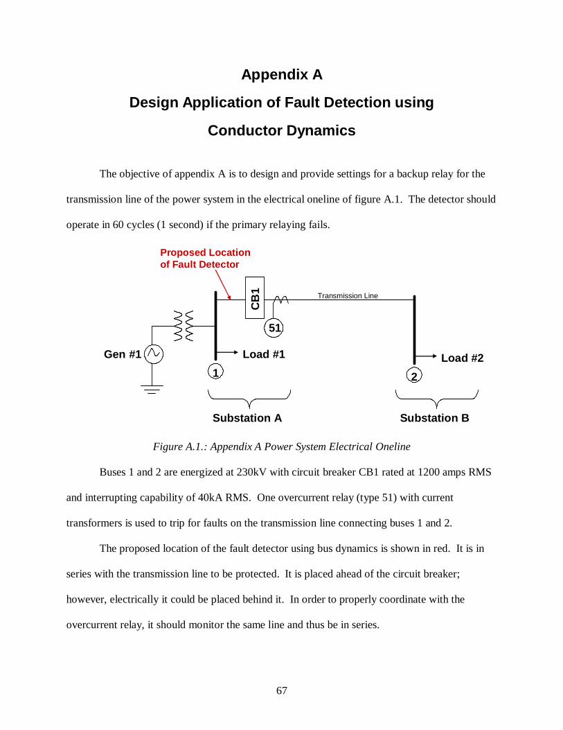
Appendix A: Design Application of Fault Detection Using Conductor Dynamics.......... 67
Page 5
iv
Appendix B: Bus Dynamic Fault Detector Design Flowchart ........................................ 87
References .................................................................................................................... 88
Vita............................................................................................................................... 90
Page 6
v
List of Figures
Figure 1.1: Typical Relay Time-Overcurrent Curves ....................................................... 2
Figure 1.2: Typical Relay and Damage Time-Overcurrent Curves................................... 3
Figure 1.3: Typical Relay and Damage Time-Overcurrent Curves w/ Backup Relays ...... 4
Figure 2.l: Circuit Model for Power System Fault Analysis ............................................. 7
Figure 2.2: Fault Current Including Transient Component ............................................. 10
Figure 2.3: Transient Fault Current Component Based on X/R Ratio............................. 11
Figure 2.4: Frequency Components of Fault Current ..................................................... 12
Figure 2.5: Example of B-Phase to Ground Fault Current.............................................. 13
Figure 2.6: Example of A-B Phase Fault Current........................................................... 14
Figure 2.7: Example of A-B Phase to Ground Fault Current .......................................... 15
Figure 2.8: Example of Three Phase Fault Current ........................................................ 16
Figure 3.1: Parallel Conductor Forces ........................................................................... 18
Figure 3.2: Input Currents 120 Degrees Out of Phase .................................................... 19
Figure 3.3: Electromagnetic Force Fab(t) ....................................................................... 20
Figure 3.4: Frequency Content of Force Fab(t) ............................................................... 21
Figure 3.5: Input Currents 120 Degrees Out of Phase with Transients ........................... 22
Figure 3.6: Electromagnetic Force Fab(t) with Transients .............................................. 23
Figure 3.7: Frequency Content of Force Fab(t) with Transients ...................................... 23
Figure 3.8: Example of Substation Three Phase Rigid Bus ............................................ 24
Figure 3.9: Three Phase Fault Current Force Vectors..................................................... 25
Figure 3.10: Example of Forces Generated for Two Fault Types ................................... 27
Page 7
vi
Figure 3.11: Bundled Fault Current Force Vectors ........................................................ 29
Figure 4.1: Beam Deflection Due to an Evenly Distributed Load................................... 33
Figure 4.2: Example of a Single Bus Span with Two Structures .................................... 34
Figure 4.3: Example of a Single Bus Span with Bundled Rigid Conductors................... 34
Figure 4.4: Spring-Mass System Representation of a Rigid Bus Span............................ 35
Figure 4.5: Magnification Factor of a Spring-Mass System ........................................... 37
Figure 4.6: Frequency Response of a Spring-Mass System............................................ 39
Figure 4.7: Natural Frequencies for Several Conductor Types ....................................... 41
Figure 4.8: Spring-Mass System Representation of a Rigid Bus Span with Insulators.... 42
Figure 4.9: Electrical Equivalent Model of a Mechanical Spring-Mass System.............. 43
Figure 4.10: Natural Frequencies of a Dual Spring-Mass System .................................. 44
Figure 4.11: Transient Step Response of a Dual Spring-Mass System............................ 45
Figure 4.12: Bundled Conductor Displacement Due to Fault Forces.............................. 47
Figure 4.13: Bundled Conductor Short Circuit Forces ................................................... 48
Figure 4.14: Transient Bundled Conductor Short Circuit Forces.................................... 50
Figure 4.15: Average Bundled Conductor Short Circuit Forces ..................................... 51
Figure 5.1: Physical Fault Detection Configuration ....................................................... 53
Figure 5.2: Electrical Diagram of Detection Logic ........................................................ 55
Figure 5.3: Profile View of Physical Fault Detection Configuration .............................. 56
Figure 5.4: Conductor Displacement with Reflecting Mirror Position............................ 57
Figure 5.5: Deflection Displacement Detection Pulses................................................... 57
Figure 5.6: Conductor Displacement Following Fault Clearing ..................................... 59
Figure 5.7: Typical Bus Dynamic Fault Detector Setting ............................................... 60
Page 8
vii
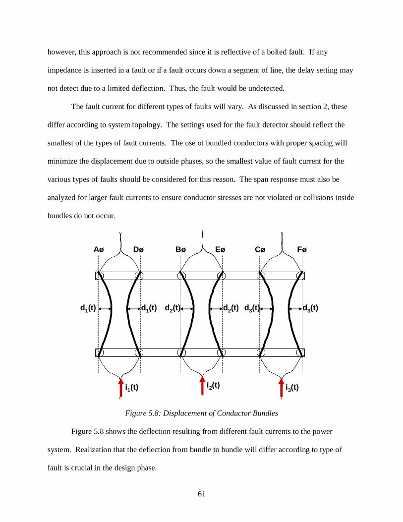
Figure 5.8: Displacement of Conductor Bundles............................................................ 61
Figure 5.9: Fault Current Contributions for Fault on Circuit 1 ....................................... 62
Figure 5.10: Fault Current Contributions for Fault on Circuit 2 ..................................... 63
Figure 5.11: Fault Current Contributions for Fault on Circuit 3 ..................................... 63
Figure 5.12: Fault Current Contributions for Fault on Circuit 4 ..................................... 64
Figure A.1: Appendix A RMS Power System Electrical Oneline ................................... 67
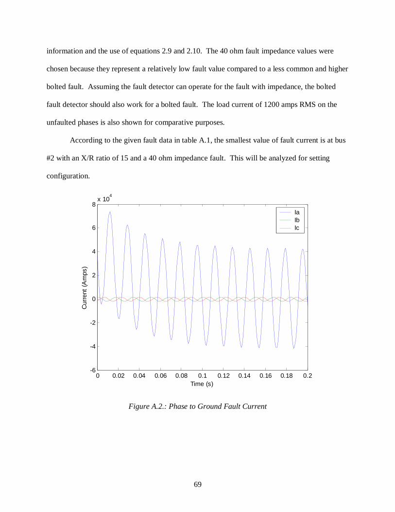
Figure A.2: Phase to Ground Fault Current.................................................................... 69
Figure A.3: Three Phase Fault Current .......................................................................... 70
Figure A.4: A Phase to Ground Fault Current Forces..................................................... 71
Figure A.5: A to B Phase Fault Current Forces.............................................................. 71
Figure A.6: A to B Phase to Ground Fault Current Forces ............................................. 72
Figure A.7: A to C Phase Fault Current Forces.............................................................. 72
Figure A.8: A to C Phase to Ground Fault Currernt Forces............................................ 73
Figure A.9: Three Phase Fault Current Forces ............................................................... 73
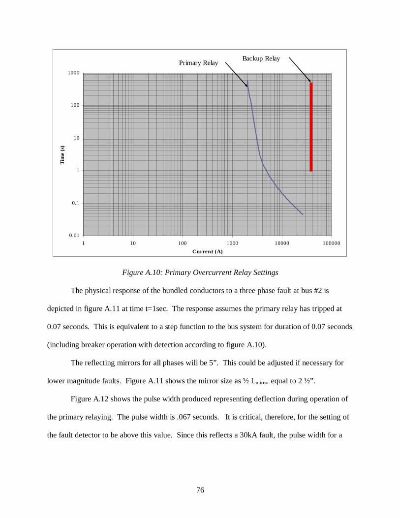
Figure A.10: Primary Overcurrent Relay Settings.......................................................... 76
Figure A.11: Conductor Deflection Using Primary Relaying ......................................... 77
Figure A.12: Pulse Width Using Primary Relaying........................................................ 77
Figure A.13: A Phase to Ground Fault Conductor Displacements.................................. 79
Figure A.14: A Phase to Ground Fault Conductor Deflection Detector Pulses ............... 79
Figure A.15: A to B Phase Fault Conductor Displacements ........................................... 80
Figure A.16: A to B Phase Fault Deflection Detector Pulses.......................................... 80
Figure A.17: A to B Phase to Ground Fault Conductor Displacements ......................... 81
Figure A.18: A to B Phase to Ground Fault Deflection Detector Pulses ......................... 81
Page 9
viii
Figure A.19: A to C Phase Fault Conductor Displacements ........................................... 82
Figure A.20: A to C Phase Fault Deflection Detector Pulses.......................................... 82
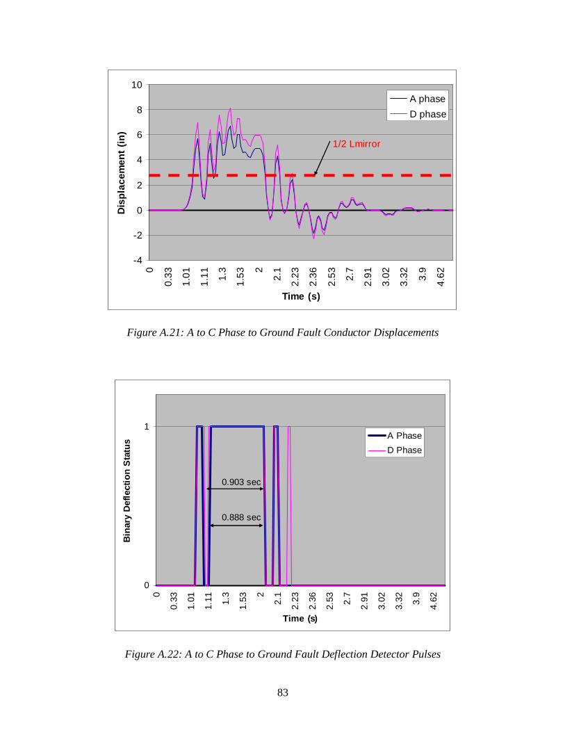
Figure A.21: A to C Phase to Phase Fault Conductor Displacements ............................. 83
Figure A.22: A to C Phase to Ground Fault .................................................................. 83
Figure A.23: Three Phase Fault A and D Bundle Conductor Displacements .................. 84
Figure A.24: Three Phase Fault A and D Bundle Deflection Detector Pulses................. 84
Figure A.25: Three Phase Fault B and E Bundle Conductor Displacements ................... 85
Figure A.26: Three Phase Fault B and E Bundle Deflection Detector Pulses ................. 85
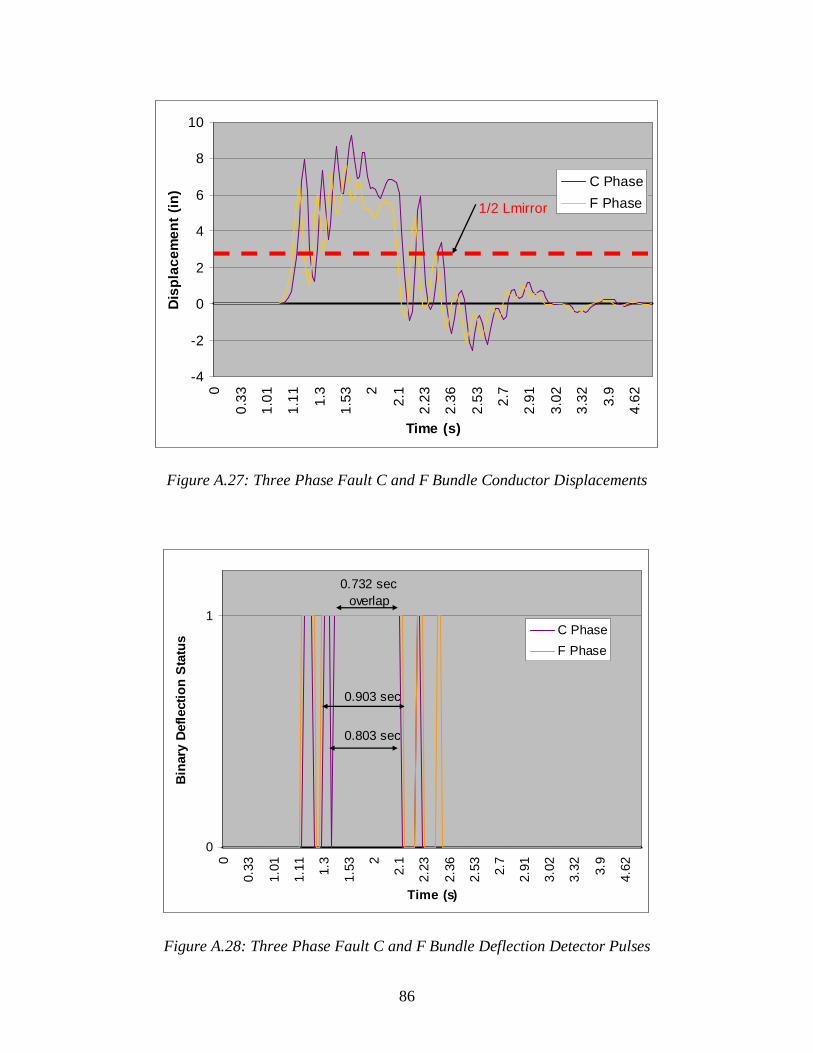
Figure A.27: Three Phase Fault C and F Bundle Conductor Displacements ................... 86
Figure A.28: Three Phase Fault C and F Bundle Deflection Detector Pulses.................. 86
Figure B.1: Design Flowchart........................................................................................ 87
Page 10
ix
List of Tables
Table 5.1: Fault Current Contributions for Various Faulted Circuits .............................. 64
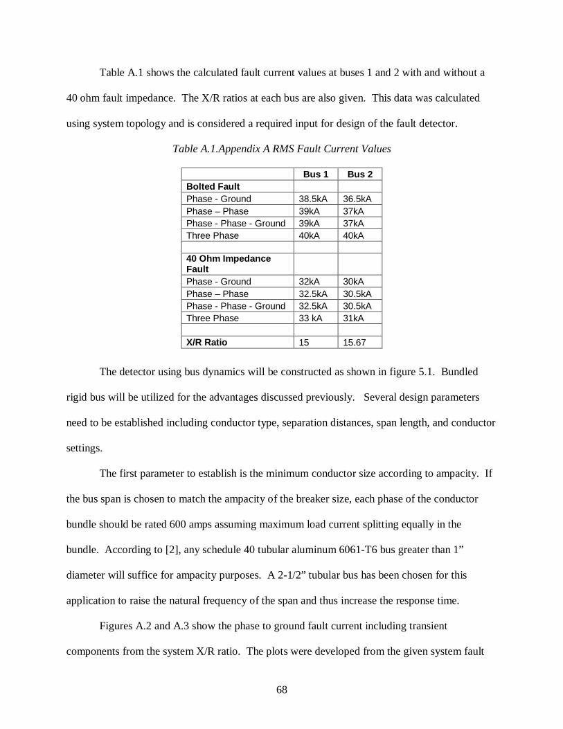
Table A.1: Appendix A Fault Current Values ................................................................ 68
Table A.2: 8A-67971A 230kV Insulator Mechanical Specifications .............................. 74
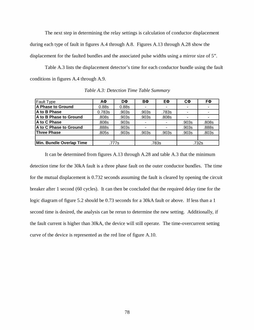
Table A.3: Detection Time Table Summary .................................................................. 78
Page 11
x
Abstract
Power system fault detection is conventionally achieved using current and potential
measurements. An alternate and unconventional form of protective relaying is feasible using
rigid bus conductor motion as the means of detection. The research presented focuses on the
detection of power system faults using visual displacement of conductor spans. Substation rigid
bus conductor motion is modeled using dual spring-mass systems for accurate representation of
conductor response to electromagnetic forces generated during system faults. Bundled rigid
conductors have advantages including detection independent of system load currents and
improved ability to detect polyphase and single phase faults. The dynamic motion of the
conductors during the fault is optically monitored with a laser detection system. Time-
overcurrent characteristics are derived for the application of fault detection. The response time
of the conductor detector system is slower than conventional relays due to the natural
frequencies of the conductor span limiting the speed of its displacement. This response time
makes the fault detection system using conductor displacement an ideal candidate for a backup
relay in power system protection schemes.
Page 12
1
1.0 Introduction
Protective relaying in power systems is crucial to safety and reliability. From the simple
household fuse to high voltage transmission line breakers, the purpose of the protective devices
is to interrupt flow effectively. This interruption results from a three step process: detect, decide,
and act.
Typical power system protective relays utilize electromechanical or microprocessor
technology to perform the three step process. Based on relay settings, the relay can detect the
fault and make a decision to trip a protective device. If the decision is made to trip, the action is
performed using a trip signal output from the relay and the circuit is opened. The critical inputs
to the protective relay are current and potential transformers connected to the monitored power
system element.
A properly protected power system has several relays with overlapping zones of
protection. The primary purpose of this is to provide adequate backup protection in the event of
improper operation. Relay settings including time and overcurrent relationships ensure proper
coordination with overlapping zones. Backup relays within the same zone provide additional
security, but often rely on the same source of electrical power and current or potential
transformers. This does, however, provide a margin of security for improperly set relays. Figure
1.1 depicts an example of l time-overcurrent curves for relay coordination.
Page 13
2
0.01
0.1
1
10
100
1000
1 10 100 1000 10000 100000Current (A)
Tim
e (s
)Primary Relay Backup Relay
Figure 1.1: Typical Relay Time-Overcurrent Curves
Inspection of figure 1.1 indicates primary relays are designed to trip before backup
relays. This is based on higher current for a shorter period of time. Typically, these values are
only attained during system faults. In the event that the primary relay does not operate as
planned, the backup relay will trip with some time delay. Overlapping zones of protection also
have similar time-overcurrent coordination curves.
Figure 1.2 includes the location of a typical power system device damage curve. It is
imperative that protective devices act prior to the damage curve or the relays will provide
inadequate protection. If the magnitude and duration of fault currents violate the damage curve,
the device needs to be repaired or replaced. Power system equipment replacement costs
Page 14
3
increases stress upon utility budgets with influence on customer rate bases. Replacement or
repair of such equipment is difficult due to the physical size and availability. Any way to avoid
equipment damage should be utilized to minimize these negative effects.
0.01
0.1
1
10
100
1000
1 10 100 1000 10000 100000Current (A)
Tim
e (s
)
Primary Relay Backup Relay Damage Curve
Figure 1.2: Typical Relay and Damage Time-Overcurrent Curves
Figure 1.3 depicts a second backup relay. This type of protection acts similar to an
overcurrent relay with time delay or a differential relay with time delay. When the current
reaches the set level, sends an instantaneous trip signal. The location of the line is determined
based on relay coordination with proper settings. The redundant backups serve as an extra layer
of protection to the power system.
Page 15
4
0.01
0.1
1
10
100
1000
1 10 100 1000 10000 100000Current (A)
Tim
e (s
)
Primary Relay Backup Relay Damage CurveBackup Relay #2
Figure 1.3: Typical Relay and Damage Time-Overcurrent Curve with Backup Relays
The intention of the research presented in this document is to present a method of backup
relay protection similar to the backup relay #2 depicted in figure 1.3. Through detailed analysis,
the novel application of conductor dynamics will be used for the purpose of fault detection. This
will be accomplished without the use of conventional equipment including electromechanical
relays, microprocessor relays, potential transformers, and current transformers. Through
deflection calculations and varied design parameters, the motion of rigid bus conductors can
provide visual indication of a power system fault and is capable of being integrated on the time-
overcurrent curves.
Page 16
5
1.1 Motivation for Research
The use of a new method of power system fault detection serves as backup protection
device with relatively low construction and maintenance costs. While the emphasis of the
research presented in this thesis is focused upon the application to power systems inside medium
to high voltage substations, the information presented can be applied in a variety of electrical
applications at various voltage levels.
1.2 Objectives of Study
The primary objective of the research presented in this paper is to provide design details
and analysis methodology for a substation design engineer to design a section of substation rigid
bus for the purpose of fault detection through visual indication.
A secondary objective to the research presented is to reveal the advantages of bundled
rigid bus in the application of fault detection using conductor dynamics.
While the design and dynamic response of substation rigid bus inside substations has
been widely studied, the research focuses on the use of dynamic analysis for bus spans [2].
Static analysis was not chosen for this research due to its limitations for the application of the
transient dynamic response.
1.3 Outline of Topics Covered
Section 2 includes the details and derivations of the transient nature of several types of
power system faults. The information presented will be used to provide an accurate dynamic
response model.
Page 17
6
Section 3 describes the dynamic motion of the bus based on deflection characteristics and
its application to rigid bus. This section also presents limitations to conventional three phase bus
configurations for its use in fault detection and lists advantages for bundled conductors.
Section 4 focuses on the dynamic analysis of bundled substation rigid bus and its analogy
to the dual spring-mass mechanical system. Emphasis is placed on natural frequencies and
variations of span components.
Section 5 describes the calibration and determination of relay settings in relay
coordination. The method chosen to detect faults uses an optical system configuration for visual
deflection indication.
Appendix A provides a detailed example of the use of conductor dynamics for the
purpose of fault detection.
Appendix B contains a flowchart to be utilized for the design of conductor bus spans to
effectively detect fault currents based on displacement. It is a practical guide for the substation
designer to effectively apply the principles presented in this research.
Page 18
7
2.0 Power System Fault Currents
Power system fault current analysis is an extensive portion of power engineering. Entire
textbooks have been written describing methodology for the detailed analysis of power system
faults. This section briefly summarizes the transient and steady state portion of fault currents.
Both of these components are necessary for the proper dynamic analysis of the substation bus
during fault conditions.
2.1 Derivation of Fault Current Components
A detailed derivation of fault current components is given in [3]. The components
derived are the steady state and transient portions of fault currents and should not be confused
with the method of symmetrical components for fault current analysis in unbalanced systems [1].
The information derived in [3] is summarized in this section.
R L
Loade(t)
FaultLocationi(t)
Figure 2.1: Circuit Model for Power System Fault Analysis
Page 19
8
The voltage source in figure 2.1 is defined in equation 2.1. The source is sinusoidal with
system frequency ( ), RMS voltage magnitude (V), and phase angle (φ ).
)tcos(V2e(t) φω += (2.1)
Analysis of the circuit in figure 2.1 with shorted load during a fault using Kirchhoff’s
voltage law yields equation 2.2.
dtdi(t)Li(t)Re(t) += (2.2)
The use of the Laplace transform and solving for i(t) assuming initial current i(0)=c in
equation 2.2 is shown in equation 2.3. N(s) is defined as the Laplace transform of cos(wt+ø).
csLR
LN(s)sLRV2i(s)
++
+= (2.3)
The inverse Laplace transform of equation 2.3 yields:
∫ ++=−−− t
0
)(tLRt
LR
)dcos(eLV2eci(t) φω (2.4)
Page 20
9
This is further evaluated by expansion of the integral to equation 2.5:
))tsin(L)tcos((RLwR
V2i(t) 222 φωωφω ++++
= (2.5)
tLRt
LR
222 ce))Lsin()tcos((ReLwR
V2 −−+++
+− φωφω
For ease of evaluation, variables and I are identified in equations 2.6 and 2.7.
RL)tan( ω
ξ −= (2.6)
222 LRVIω+
= (2.7)
Substitution of equations 2.6 and 2.7 into 2.5 is shown in equation 2.8.
tLR
)]ecos(I2[c)tcos(I2i(t)−
+−+++= φφω (2.8)
Inspection of equation 2.8 reveals both the steady state (equation 2.9) and transient
(equation 2.10) components of the fault current.
)cos(wtI2i(t) esteadystat ++= φ (2.9)
]e))cos(I2[ci(t)t
LR
transient−
+−= φ (2.10)
Page 21
10
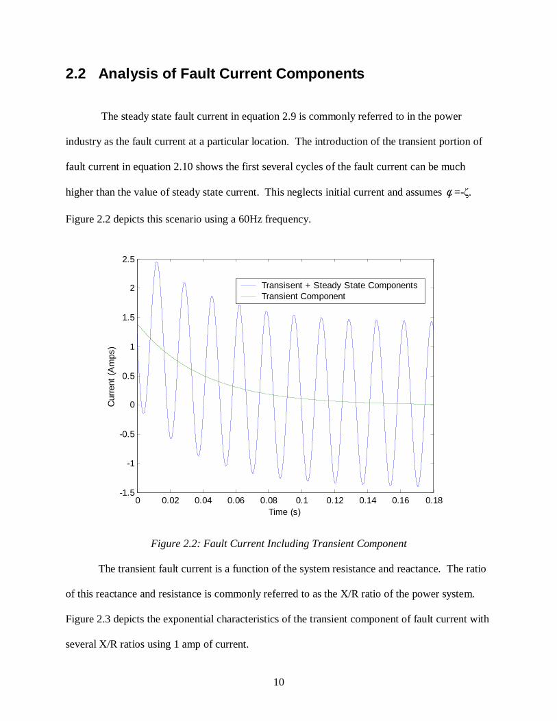
2.2 Analysis of Fault Current Components
The steady state fault current in equation 2.9 is commonly referred to in the power
industry as the fault current at a particular location. The introduction of the transient portion of
fault current in equation 2.10 shows the first several cycles of the fault current can be much
higher than the value of steady state current. This neglects initial current and assumes φ =- .
Figure 2.2 depicts this scenario using a 60Hz frequency.
0 0.02 0.04 0.06 0.08 0.1 0.12 0.14 0.16 0.18-1.5
-1
-0.5
0
0.5
1
1.5
2
2.5
Time (s)
Cur
rent
(Am
ps)
Transisent + Steady State ComponentsTransient Component
Figure 2.2: Fault Current Including Transient Component
The transient fault current is a function of the system resistance and reactance. The ratio
of this reactance and resistance is commonly referred to as the X/R ratio of the power system.
Figure 2.3 depicts the exponential characteristics of the transient component of fault current with
several X/R ratios using 1 amp of current.
Page 22
11
0 0.05 0.1 0.15 0.2 0.25 0.3 0.350
0.5
1
1.5
Time (s)
Cur
rent
(Am
ps)
X/R=5X/R=10X/R=15X/R=20X/R=25X/R=30X/R=35
Figure 2.3: Transient Fault Component Based on System X/R Ratio
Inspection of figure 2.3 and equation 2.10 indicates that the magnitude of the fault current
transient component is the same at the initiation of the fault for any X/R ratio. It decays slower
with a higher X/R ratio than a low one. The response of the bus to the system fault current and
its generated forces is a function of this X/R ratio.
The X/R ratio is a function of fault location. A fault near a transformer generally has a
high X/R ratio due to the windings of the transformer and its impact in increasing the reactance
at the fault location. This increased reactance will slow the transient decay time in comparison
with a low voltage distribution feeder with a smaller X/R ratio and shorter decay time. Any use
of protective relaying should consider this X/R ratio for the instantaneous and transient fault
current considerations.
Page 23
12
The frequency components of fault currents including transient components can be
attained using Fourier analysis. The primary frequencies are 60Hz with a DC component.
Figure 2.4 depicts the components for the first 11 msec of the time domain signal in figure 2.2.
The Fourier transform of the waveform of this time domain signal is defined as:
+
++
+=
LR
)cos(I2w)(G 2o
2o φ .
0 50 100 150 200 250 300 350 400 450 5000
0.1
0.2
0.3
0.4
0.5
0.6
0.7
0.8
0.9
1
|G(w
)|
Frequency (Hz)
Transient + Steady State Fault Current
Figure 2.4: Frequency Components of Fault Current
Page 24
13
2.3 Types of Power System Faults
The four primary types of faults are detailed in [1]. These include phase to
ground, phase to phase, phase to phase to ground, and three phase. The use of symmetrical
component analysis described in [1] proves beneficial for calculation of each type of fault.
It is critical that the protection designed for the power system respond to each possible
fault condition. While the power system designer can account for several different types of
faults, the protective equipment may not be able to distinguish between the various types of
faults. An accurate system model for studying power system faults including correct system
impedance parameters will minimize calculated fault current errors.
An example of the B phase to ground fault is depicted in figure 2.5 using an X/R ratio of
15, fault current magnitude of 20kA RMS, and load current of 2kA RMS. Symmetry of
approximately 120 degrees between phases is maintained through the fault duration.
0 0.02 0.04 0.06 0.08 0.1 0.12 0.14 0.16 0.18-3
-2
-1
0
1
2
3
4
5x 10
4
Time (s)
Cur
rent
(A
mps
)
A phaseB phaseC phase
Figure 2.5: Example of B-Phase to Ground Fault Current
Page 25
14
An example of a phase to phase fault is shown in figure 2.6. The same assumptions used
in figure 2.5 have been used for depiction of the fault. Because the fault current does not include
a ground path, the two faulted phases are symmetric in steady state magnitude as indicated in [6].
While the transient component is shown as identical for both phases, the transient portion of each
phase may not actually be identical as indicated in [2]. The phase angle of the C phase current
relative to A phase is a function of system topology and varies with system locations.
0 0.02 0.04 0.06 0.08 0.1 0.12 0.14 0.16 0.18-3
-2
-1
0
1
2
3
4
5
6x 10
4
Time (s)
Cur
rent
(Am
ps)
A phaseB phaseC phase
Figure 2.6: Example of A to B Phase Fault Current
The introduction of the ground path in the phase to phase fault depicted in figure 2.6
removes the symmetry of the faulted phases as indicated in figure 2.7 using the same
assumptions. Actual phase angles and transient component contributions will vary according to
system topology as previously described.
Page 26
15
0 0.02 0.04 0.06 0.08 0.1 0.12 0.14 0.16 0.18-3
-2
-1
0
1
2
3
4
5
6x 10
4
Time (s)
Cur
rent
(Am
ps)
A phaseB phaseC phase
Figure 2.7: Example of A to B Phase to Ground Fault Current
Three phase faults provide phase angles of approximately 120 degrees as indicated in
figure 2.8. Similar to phase to phase and phase to phase to ground faults, actual transient
components for faulted phases vary with system topology. The magnitudes of the faulted phase
currents are equal assuming a balanced three phase system. The introduction of the ground path
in three phase faults does not alter the fault currents.
Page 27
16
0 0.02 0.04 0.06 0.08 0.1 0.12 0.14 0.16 0.18-3
-2
-1
0
1
2
3
4
5
6x 10⁴
Time (s)
Cur
rent
(A
mps
)A phaseB phaseC phase
Figure 2.8: Example of Three Phase Fault Current
The purpose of identifying the various types of system faults is to ensure the proposed
methods of relaying encompass all types of faults. The simple flow of too much current on an
electrical device can cause heat, flames, equipment damage, and lethal ground potential rise. A
protection scheme not encompassing every fault scenario provides additional risk to equipment,
personnel, and the general public.
Page 28
17
3.0 Fault Current Forces
Extensive studies have been performed on substation rigid bus using various static and
dynamic models. This section describes methodology for both static and dynamic analysis of
fault current forces between rigid bus conductors. The conclusion is made that the dynamic
modeling of electromechanical forces provides a more accurate representation of actual forces
generated than static forces.
3.1 Electromagnetic Conductor Forces
The magnetic force on a current carrying wire is detailed in [7]. The equations used in
this section are primarily obtained from [7] with application to the motion of bus relevant to fault
current response.
The force vector due to electromagnetism on a conductor is defined in equation 3.1. The
force is dependent upon the conductor length, magnetic field generated, and applied current.
BLiFvvv
⊗= (3.1)
Equation 3.1 applied to the scenario of two parallel conductors depicted in figure 3.1
yields a cross product which can be reduced to equation 3.2, based on the parallel nature of the
design.
cos(0)BLiF abab = (3.2)
The magnetic field contribution from conductor A, Ba at wire B is defined in equation 3.3
where the permeability constant of air is 7o 10−×= and d is the distance between conductors.
d2iB ao
a = (3.3)
Page 29
18
Substitution of equation 3.3 into equation 3.2 with time varying input currents yields
equation 3.4. The output force vector is a function of time based on time and direction of the
input currents.
d2(t)i(t)iL(t)F bao
ab
vvv
= (3.4)
Two parallel conductors are depicted in figure 3.1. Currents are injected into the two
conductors with magnitudes (t)Iav
and (t)Ibv
. The direction convention of equation 3.4 is noted in
figure 3.1. The force on each conductor is identical in magnitude such that baab FF = .
Direction is dependent upon the direction of current as described in [7].
Ia(t)
Ib(t)
Fab(t)
Fba(t)
L d
Figure 3.1: Parallel Conductor Forces
If the currents (t)Iav
and (t)Ibv
are in the same direction, the resulting force vector
(t)Fabv
produces a pinch effect where the two conductors are pulled together. On the contrary,
currents in opposite directions produce repelling forces. The use of DC current produces static
Page 30
19
forces on conductors where AC currents produce dynamic forces with points of zero force at the
zero crossing of either input, (t)Iav
or (t)Ibv
.
In the electric utility, the use of static (DC) forces are not as common due to a primarily
AC dominated power grid. [1] explains the use of voltage vectors with their 120 degree phase
separation in the electric grid. Consider, for example, figure 3.1 with input currents separated
with a phase angle of 120 degrees as indicated in figure 3.2. This configuration is similar to two
phases of a distribution line without the presence of the third. The application of equation 3.4
with separation distance d = 1 ft and current magnitude of 1kA produces the dynamic force
(#/inch) as indicated in figure 3.3.
0 0.01 0.02 0.03 0.04 0.05 0.06 0.07 0.08-1500
-1000
-500
0
500
1000
1500
Time (s)
Cur
rent
(A
mps
)
Ia(t)Ib(t)
Figure 3.2: Input Currents 120 Degrees Out of Phase
Page 31
20
0 0.01 0.02 0.03 0.04 0.05 0.06 0.07 0.08-12
-10
-8
-6
-4
-2
0
2
4x 10⁻³
Time (s)
Fab(
t) (#
/in)
Figure 3.3: Electromagnetic Force Fab(t)
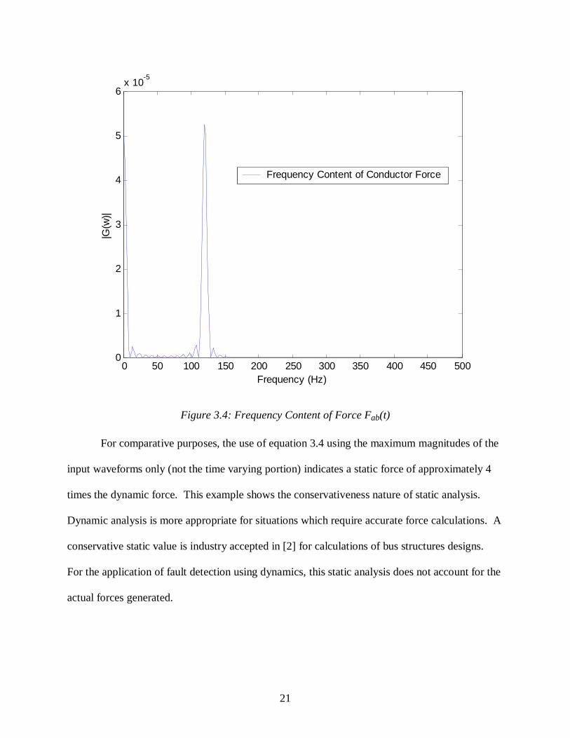
Figure 3.3 shows a sinusoidal force with positive and negative portions at its force
frequency. This force frequency is twice that of the power frequency. A Fourier analysis of the
frequency content is shown in figure 3.4. For the case of the 60 Hz power frequency, the
frequency of force is 120Hz with a DC component. The Fourier transform is defined as:
+
+=
1d2ILG(w) 2
o2
2o .
Page 32
21
0 50 100 150 200 250 300 350 400 450 5000
1
2
3
4
5
6x 10⁻⁵
|G(w
)|
Frequency (Hz)
Frequency Content of Conductor Force
Figure 3.4: Frequency Content of Force Fab(t)
For comparative purposes, the use of equation 3.4 using the maximum magnitudes of the
input waveforms only (not the time varying portion) indicates a static force of approximately 4
times the dynamic force. This example shows the conservativeness nature of static analysis.
Dynamic analysis is more appropriate for situations which require accurate force calculations. A
conservative static value is industry accepted in [2] for calculations of bus structures designs.
For the application of fault detection using dynamics, this static analysis does not account for the
actual forces generated.
Page 33
22
The presence of a transient component in fault current forces produces non-sinusoidal
force waveforms until the transient components decay. Figure 3.5 depicts the input current
waveforms of figure 3.2 including a transient portion with X/R = 15.
0 0.02 0.04 0.06 0.08 0.1 0.12 0.14 0.16 0.18 0.2-1500
-1000
-500
0
500
1000
1500
2000
2500
3000
Time (s)
Cur
rent
(A
mps
)
Ia(t)Ib(t)
Figure 3.5: Input Currents 120 Degrees Out of Phase with Transients
Figure 3.6 shows the electromagnetic force waveform for the two currents presented in
figure 3.5. After the transient forces decay, the steady state waveform is identical to figure 3.3.
Its associated frequency spectrum for the first 11msec is shown in figure 3.7. The Fourier
transform is defined as:
+
++
+
+=
LR
)cos(121
dIL
G(w)2
o2
2o φ .
Page 34
23
0 0.02 0.04 0.06 0.08 0.1 0.12 0.14 0.16 0.18 0.2-0.015
-0.01
-0.005
0
0.005
0.01
0.015
0.02
0.025
Time (s)
Fab(
t) (#
/in)
Figure 3.6: Electromagnetic Force Fab(t) with Transients
0 50 100 150 200 250 300 350 400 450 5000
0.2
0.4
0.6
0.8
1
1.2
1.4
1.6
1.8x 10
-4
|G(w
)|
Frequency (Hz)
Frequency Content of Conductor Force
Figure 3.7: Frequency Content of Force Fab(t) with Transients
Page 35
24
During the decay, a 60Hz force contribution is present. A similar peak 120Hz force is
most apparent with contributions from a DC portion. Inspection of figure 3.6 indicate the first
several cycles more closely resemble a 60Hz waveform than a 120Hz one. The necessity for the
use of the transient 60Hz and DC component will become apparent on the discussion of bus
response in section 4.
3.2 Three Phase Electromagnetic Conductor Forces
The use of three phase electric systems is common throughout the power industry. The
infrastructure for the power grid particularly in substations and transmission lines, revolves
around construction of sets of three identical phases. Figure 3.8 depicts a typical substation bus
with insulator supports1.
Aluminum TubeRigid Bus
Insulator
Support Structure
Figure 3.8: Example of Substation Three Phase Rigid Bus
1 Photo courtesy of Entergy Services, Inc.
Page 36
25
Figure 3.8 depicts a single support structure to which three station post insulators are
attached. The insulators are in line to support rigid bus tubing using a bus clamp. Multiple spans
of bus are used to carry current to electrical devices inside the substation. The substation
designer has the flexibility to utilize multiple structures, insulators, and busbar according to
electrical and physical constraints for the construction of substation bus. Figure 3.8 is one
possible configuration which should be analyzed in detail by the substation designer. Design
forces characterized for substation rigid bus in [2] include ampacity, corona, vibration,
gravitational, wind, fault current, expansion, insulator, and conductor.
The various forces acting on substation bus spans add as vectors. Figure 3.9 depicts the
net fault current forces for a plan view of a typical three phase span of bus. The forces are
depicted at different points along the conductor for clarity purposes; however, the forces actually
are evenly distributed on the bus as described in section 3.1.
FAC(t)
Cø
FAB(t)
Bø
FAB(t)
Aø
FAC(t)
FBC(t)FBC(t)
Figure 3.9: Three Phase Fault Current Force Vectors
Assuming the positive X direction is from the A phase towards the C phase, the net force
for the three phases are defined in equations 3.5 through 3.7.
Page 37
26
(t)F(t)F(t)F ACABAvvv
+= (3.5)
(t)F(t)F(t)F BCABBvvv
−= (3.6)
(t)F(t)F(t)F BCACCvvv
−−= (3.7)
3.3 Single Conductor Three Phase Rigid Bus
Due to the unpredictable nature of faults and their seemingly random phase selection, any
protection system should be able to detect any type of fault at any moment in time. This holds
true for optical detection based conductor deflection. The conductor must deflect noticeably for
any type of fault possible. Contributions from other phases have significant influence on this
deflection. This section discusses the electromagnetic force influences from each conductor
during the fault.
Inspection of equation 3.4 reveals a dependence upon the dynamic parameters of
(t)Iav
and (t)Ibv
. For load current magnitudes much smaller than fault current magnitudes, the
force between phases is extremely small and can generally be neglected. Since these fault
current magnitudes are much higher than load currents, it is the scenario of a fault for which
forces become significant enough to move the bus and allow for visual fault detection.
The ratio of the static force produced in a phase to phase fault using equation 3.4 versus a
phase to ground fault is the ratio of fault current to load current of the unfaulted phase. Using
dynamic analysis, the ratio can be calculated as indicated in the example below. Due to the
unpredictable nature of faults, it is possible for a conductor to see significantly less force for a
phase to ground fault than a phase to phase one. The ability to visually distinguish a fault using
conductor dynamics becomes challenging from a design perspective. The dependence of A and
Page 38
27
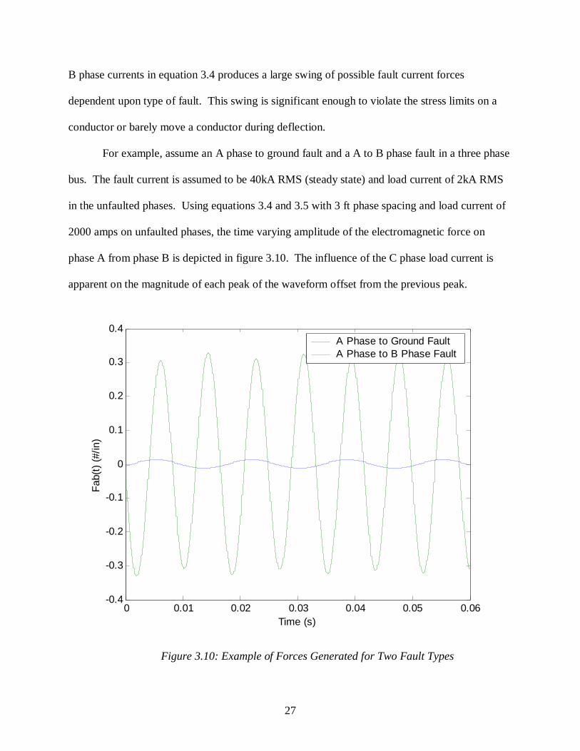
B phase currents in equation 3.4 produces a large swing of possible fault current forces
dependent upon type of fault. This swing is significant enough to violate the stress limits on a
conductor or barely move a conductor during deflection.
For example, assume an A phase to ground fault and a A to B phase fault in a three phase
bus. The fault current is assumed to be 40kA RMS (steady state) and load current of 2kA RMS
in the unfaulted phases. Using equations 3.4 and 3.5 with 3 ft phase spacing and load current of
2000 amps on unfaulted phases, the time varying amplitude of the electromagnetic force on
phase A from phase B is depicted in figure 3.10. The influence of the C phase load current is
apparent on the magnitude of each peak of the waveform offset from the previous peak.
0 0.01 0.02 0.03 0.04 0.05 0.06-0.4
-0.3
-0.2
-0.1
0
0.1
0.2
0.3
0.4
Time (s)
Fab(
t) (#
/in)
A Phase to Ground FaultA Phase to B Phase Fault
Figure 3.10: Example of Forces Generated for Two Fault Types
Page 39
28
The static ratio of fault current force is 20. Dynamically at an instant in time, however,
the ratio is approximately 22. Inclusion of the ground path in the fault or a three phase fault
produces similar ratios. In either the static or dynamic analysis, it is clear in figure 3.10 that the
ratio of force generated can be large depending upon which type of fault occurs for a system.
3.4 Bundled Conductor Three Phase Rigid Bus
The use of bundled rigid conductors is generally not common in substations. Typically,
bundled conductors are used on transmission lines or jumper conductors which require additional
ampacity or to reduce the effects of audible corona on EHV substations. Conductor sizing is
generally based on heat rate for each installation (ampacity) and available hardware for the
conductors chosen. The rigid bus ampacity values from single conductors are usually sufficient
for heating due to load currents. The additional hardware and construction time are generally
unnecessary. Overall, the concept has not been utilized much inside the substation.
The use of bundled rigid conductors has a distinct advantage for fault detection purposes
which will be analyzed in this section and in section 4. These include conductor deflection
independent of unfaulted phase load current values or type of fault. Symmetry of the bundle
requires deflection of both phases to prevent false trips due to natural phenomenon such as
animal interference with the detection device.
As depicted in figure 3.10, the electromagnetic force differences from phase to phase and
phase to ground faults can be high. The deflection differences of each type of fault are
substantial enough to limit the detection of the fault depending upon conditions. Section 4 will
discuss this in detail.
Page 40
29
Equation 3.4 shows the dependence on load current in unfaulted phases to produce
electromagnetic forces. Thus, low load faults versus high load faults will produce different
forces on the conductors. Deflection of the bus is affected by this load current. A fault detection
system should be able to properly detect faults for any load level. This reality limits the use of
conventional three phase, single conductor bus designs.
Figure 3.11 depicts a plan view of the electromagnetic forces using a six conductor, three
phase bundled bus. As in figure 3.9, the forces are depicted at different points along the
conductor for clarity purposes; however, the forces actually are evenly distributed on the
conductors. It should be noted that phases A and D, B and E, C and F are equipotential and
bundled.
FAB(t)Aø
FAC(t)
FAD(t)
FAE(t)
FAF(t)
FDB(t)Dø
FDC(t)
FDE(t)
FDF(t)
FAD(t)
Bø
FBE(t)
FBC(t)
FBF(t)
Eø
FEF(t)
FBE(t)
Cø
FCF(t)
Fø
FCF(t)
FAB(t)
FDB(t)
FDE(t)FEC(t)
FAE(t) FBF(t)
FEF(t)
FDF(t)
FAF(t)
FBC(t)
FAC(t)
FDC(t)
FEC(t)
d d d
S S
Figure 3.11: Bundled Fault Current Force Vectors
Each bundled conductor depicted in figure 3.11 is separated by a distance d. Each bundle
is separated by distance S. Assuming the bundles are equipotential with equal current
distribution, the force seen on each conductor bundle is symmetric and independent of which
Page 41
30
type of fault is present in the system, neglecting the contributions from other phases. The net
force on the bundles including outside phases is listed in equations 3.8 through 3.13.
Assuming the positive X direction is from the A phase towards the C phase, the net force
for the three phases are defined as:
(t)F(t)F(t)F(t)F(t)F(t)F AFAEADACABAvvvvvv
++++= (3.8)
(t)F(t)F(t)F(t)F(t)F(t)F ADDFDEDCDBDvvvvvv
−+++= (3.9)
(t)F(t)F(t)F(t)F(t)F(t)F DBABBFBCBEBvvvvvv
−−++= (3.10)
(t)F(t)F(t)F(t)F(t)F(t)F DEBEAEEFECEvvvvvv
−−−+= (3.11)
(t)F(t)F(t)F(t)F(t)F(t)F ECDCBCACCFCvvvvvv
−−−−= (3.12)
(t)F(t)F(t)F(t)F(t)F(t)F EFDFCFBFAFFvvvvvv
−−−−−= (3.13)
Application of equation 3.4 to the bundled conductors in figure 3.11 indicates that the
closer two conductors are, the stronger their electromagnetic force generated. Thus, the force on
phase A from phase F will be significantly less than that of phase A on phase D. In order to
utilize the bundled configuration to accurately detect faults based on deflection due to bus
dynamics, the design should try to keep d<<S as depicted in figure 3.11. This will increase the
bundle isolation and create a response with negligible effects from load currents on unfaulted
phases.
Electromagnetic forces due to the pinch effect can be extreme and must be analyzed for
any possible violation of conductor stress limits. Equation 3.14 shows the maximum span length
for a conductor with two pinned ends as given in [2]. C is 3.46 for English units, Ls is the
maximum allowable span length (inches), FA is the maximum allowable stress (lb/in), S is the
Page 42
31
total section modulus (in3), and FT is the total force (lb/ft). The maximum stress is typically the
elastic limit of the material.
T
As F
SF12CL = (3.14)
In addition to stress limits determining the maximum separation distance of a
conductor bundle, the deflection of the conductor under stress due to the electromagnetic forces
must be considered. Clearly, the two conductors should not be close enough to collide into each
other as the deflection occurs. Such a scenario could damage the conductor or structure. Section
four discusses time varying bus deflection in detail.
Page 43
32
4.0 Substation Bus Response
In order to accurately detect system faults using conductor dynamics, the response of the
conductor to the electromagnetic forces must be accurately analyzed.
Like the static and dynamic analyses of the electromagnetic forces in section 3, the
mechanical response will be analyzed in this section. The use of both static and dynamic
responses of the substation rigid bus will be discussed.
4.1 Static Analysis of Rigid Bus Mechanical Response
Static mechanical analysis for a dynamic natured system will produce conservative
results independent of time. In reality, this approach is commonly used for the selection of bus
materials. The information provided in [2] is based mostly from this static analysis. The
conservative results are used to provide for a margin of safety in the selection of substation
materials.
These conservative results also neglect the time variable. As described in sections 2 and
3, the time variable is critical in the use of fault detection.
In the simple case of a single span of bus, the following example describes the simplicity
yet inaccuracy of strict static analysis when accurate, time dependent results are necessary.
The deflection of a single span of rigid bus with tightly clamped bus on insulators can be
modeled as a beam with a constant load applied as seen in figure 4.1 per [8].
Page 44
33
L
d
w
Figure 4.1: Beam Deflection Due to an Evenly Distributed Load
The uniform load, w (#/in), shown in figure 4.1, produces a beam deflection at the
midspan of the beam of length L (in) given in equation 4.1 where E is the modulus of elasticity
(#/in2) and I is the moment of inertia (in4).
IE384Lwd
4= (4.1)
If a static load, w, is applied to this simple beam, the beam moves from its at rest position
to its newly deflected position and remain until the load is removed. This approach of static
analysis does not account for any time delay required for the beam to get from its at rest position
to its deflected one. If accurate time based fault detection is required, this method is inadequate.
Dynamic analysis is selected to improve this accuracy.
This is merely one example of a single span of bus deflection. The substation designer
has the flexibility to vary the number of spans and conductor types according to substation
requirements. The methods for analysis of these are given in [2]. The use of the single
conductor span with two support insulators will be commonly used throughout this paper (figure
4.2). Implementation of the methodology used in this paper allows for the flexibility of
mounting structure dimension and spans using the single span as a starting point for the design.
Page 45
34
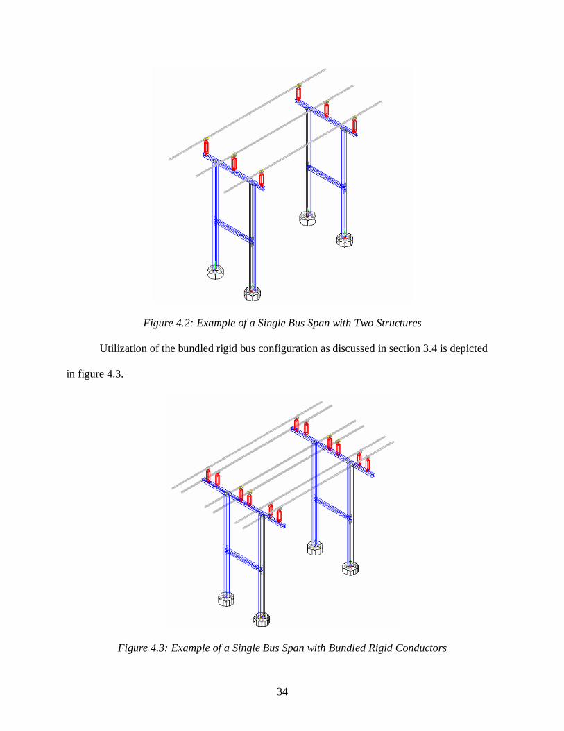
Figure 4.2: Example of a Single Bus Span with Two Structures
Utilization of the bundled rigid bus configuration as discussed in section 3.4 is depicted
in figure 4.3.
Figure 4.3: Example of a Single Bus Span with Bundled Rigid Conductors
Page 46
35
4.2 Dynamic Analysis of Rigid Bus Mechanical Response
The dynamic analysis of substation rigid bus is best accomplished using the analogy of a
spring-mass system. The deflection shown in figure 4.1 has a time component dependent upon
the natural frequency of the span. Figure 4.4 depicts a simple spring model of a conductor span
where k is the spring constant, m is the system mass, P(t) is the applied force, and x(t) is the
displacement.
m
k
mP(t)
x(t)
k
Figure 4.4: Spring-Mass System Representation of Rigid Bus Span
The dynamic analysis of the simple spring mass system is detailed in [9] and modeled by
the differential equation 4.2.
t)sin(Pkxdt
xdm f2
2ω=+ (4.2)
Because it has one degree of freedom, the X direction will be used to indicate motion of
the mass. On the rigid conductor spans depicted in figures 4.2 and 4.3, the direction of force is
perpendicular to the ground plane. The driving force, P(t) is defined as a sinusoidal waveform
Page 47
36
with forced frequency, f . In the case of a power system fault, the driving forces are the
electromagnetic forces described in section 3.2.
Solving equation 4.2 for displacement, x(t), results in equation 4.3 where P is the
amplitude of the driving force and n is the system natural frequency.
2
nf1
kPx(t)
−
= (4.3)
The natural or circular system frequency is defined in equation 4.4. It is independent of
any outside forces and is the time required for steady state deflection to occur.
mk
n = (4.4)
The driving frequency should not be confused with the system natural frequency. The
system can be excited using any value of P(t) with distinct driving frequencies. In the case of the
span of rigid bus on the 60 Hz power grid as described in previous sections, these are primarily
120 Hz with a DC offset with some 60 Hz components dependent upon the system X/R ratio.
[10] discusses the concept of a magnification factor. The ratio of the displacement, x(t),
to the static displacement, -kx, is a magnification factor, (sigma), described in equation 4.5.
2
nf1
1
kPx(t)
−
== (4.5)
Further analysis of equation 4.5 reveals an asymptote when the forced frequency is equal
to the natural frequency. Figure 4.5 depicts this asymptote and the magnification factor.
Page 48
37
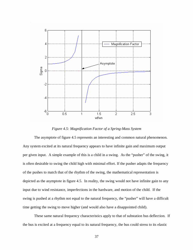
Figure 4.5: Magnification Factor of a Spring-Mass System
The asymptote of figure 4.5 represents an interesting and common natural phenomenon.
Any system excited at its natural frequency appears to have infinite gain and maximum output
per given input. A simple example of this is a child in a swing. As the “pusher” of the swing, it
is often desirable to swing the child high with minimal effort. If the pusher adapts the frequency
of the pushes to match that of the rhythm of the swing, the mathematical representation is
depicted as the asymptote in figure 4.5. In reality, the swing would not have infinite gain to any
input due to wind resistance, imperfections in the hardware, and motion of the child. If the
swing is pushed at a rhythm not equal to the natural frequency, the “pusher” will have a difficult
time getting the swing to move higher (and would also have a disappointed child).
These same natural frequency characteristics apply to that of substation bus deflection. If
the bus is excited at a frequency equal to its natural frequency, the bus could stress to its elastic
Page 49
38
limits and create permanent damage. The major means of excitement for rigid bus are seismic,
wind, and electromagnetic. In general, it is desirable to design substation equipment such that
the natural frequencies of conductor spans do not have a chance of becoming excited with a large
magnification factor by any of these forces. For electromagnetic force excitement, the IEEE
recommends the use of dampers if the natural frequency of the conductor span is greater than the
power frequency [2]. Additionally, if twice the natural frequency of a span is greater than the
force driving frequency due to wind, damping is recommended. Damping commonly involves
the installation of flexible conductor inside a tubular conductor.
On the other hand, the natural frequency presents unique design characteristics. For
example, [11] presents the novel application of removal of ice from flexible bundled conductors
by exciting the span with frequencies near its fundamental frequency. This oscillatory
excitement causes conductor bundles to literally collide with each other and remove ice by these
collisions.
In the application of fault detection, the natural frequency of the bus span plays a key
role. In accordance with the magnification factor described in this section, the ratio of the
driving frequency to the rigid bus span’s natural frequency will be greater than unity. As in the
analogy of a child on a swing, the theoretical value of infinite gain cannot be reached by the
conductor driven at its natural frequency. This is mostly due to the resistance of the bus supports
and insulator supports and the damping it provides. Although this infinite gain characteristic
cannot be attained, it still represents the frequencies producing the most stress on the span.
Figure 4.6 depicts a typical frequency response output for the spring mass system
depicted in figure 4.4. The peak gain is not infinite for the reasons described in this section. The
natural frequency of the system is approximately 4.5 Hz.
Page 50
39
0
2
4
6
8
10
12
14
16
1 2 3 4 5 6 7 8 9 10 11 12 13 14 15 16 17 18
Frequency (Hz)
Gai
n (O
utpu
t/Inp
ut)
Frequency Content
Rolloff
Figure 4.6: Frequency Response of a Spring-Mass System
The components of rigid bus spans must be translated to parameters of the spring-mass
models for the purpose of dynamic analysis.
The natural frequency of a single bus span with fixed ends is defined in equation 4.6 as
described in [2].
mEI
LCKf 2
2n = (4.6)
where fn = natural frequency of conductor span
K = 1.51 for fixed ends on the conductor span
C = 24 for English units
L = conductor length (ft)
E = modulus of elasticity (lb/in2)
I = moment of inertia (in4)
m = mass per unit length (lb/ft)
Page 51
40
The conductor spring constant, kbus, is determined by combining equations 4.4 and 4.6
into equation 4.7.
IELCK4k 42
44bus = (4.7)
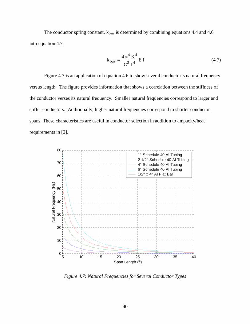
Figure 4.7 is an application of equation 4.6 to show several conductor’s natural frequency
versus length. The figure provides information that shows a correlation between the stiffness of
the conductor verses its natural frequency. Smaller natural frequencies correspond to larger and
stiffer conductors. Additionally, higher natural frequencies correspond to shorter conductor
spans These characteristics are useful in conductor selection in addition to ampacity/heat
requirements in [2].
5 10 15 20 25 30 35 400
10
20
30
40
50
60
70
80
Nat
ural
Fre
quen
cy (
Hz)
Span Length (ft)
1" Schedule 40 Al Tubing2-1/2" Schedule 40 Al Tubing4" Schedule 40 Al Tubing6" Schedule 40 Al Tubing1/2" x 4" Al Flat Bar
Figure 4.7: Natural Frequencies for Several Conductor Types
Page 52
41
The analogy of the spring-mass system should include the support insulators. Tips of the
insulators will move at their natural frequencies when driving forces are applied. [12] describes
the concept of a spring constant for insulator supports. This insulator spring constant is defined
in equation 4.8 where E is the section modulus, I is the moment of inertia, and H is the height of
the insulator.
HIE3kins = (4.8)
Equation 4.9 gives the natural frequency for insulators. In reality, this natural frequency
is the basis for determining tip displacement versus applied load to a span of conductor. Both the
natural frequencies for the bus span and insulator have been verified using the chirp response
method via adaptive filtering in [12].
bi
insins FF.226
gk1f+
= (4.9)
where fins = insulator natural frequency
g = gravitational constant (386.4 in/s2)
Fi = insulator weight (lb)
Fb = effective weight of conductor transmitted to support fitting (lb)
The dynamic model for a single span of bus including the response of the insulators is
depicted in figure 4.8.
Page 53
42
m1
kins
m1
x1(t)
m2
kbus
m2
P(t)
x2(t)
kbus
kins
Figure 4.8: Spring-Mass System Representation of Rigid Bus Span with Insulators
The dual spring-mass system of figure 4.8 can be electrically analyzed using the model in
figure 4.9.
L1=m1
+x2(t)
L2=m2
C1=1/kinsC2=1/kbusP(t)-
+
-
+
-
Rdamp
Figure 4.9: Electrical Equivalent Model of a Mechanical Spring-Mass System
The damping resistor, Rdamp has been included in the electrical model to dampen the
response of the linear system. Without such a resistor, the energy due to friction of supports and
Page 54
43
wind resistance would not dissipate any of the energy from the input source. This produces a
ringing effect which would never settle to any DC value.
The differential equations governing the electrical equivalent circuit are shown in
equations 4.10 and 4.11 (neglecting the resistance contribution). The mechanical system
equivalents are shown in equations 4.12 and 4.13.
0C
qqCq
dtqdL
2
21
1
121
21 =
−++ (4.10)
P(t)C
qqdt
qdL2
1222
22 =
−+ (4.11)
0)x(xk xkdt
xdm 2121121
21 =−++ (4.12)
P(t))x(xkdt
xdm 12222
22 =−+ (4.13)
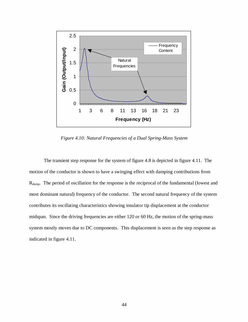
The frequency response of the dual spring-mass system, figure 4.10, shows the presence
of two distinct natural frequencies. The smaller natural frequency is the conductor span’s
frequency and the larger is the insulator natural frequency. This is consistent with the
conclusions in [12].
Page 55
44
0
0.5
1
1.5
2
2.5
1 3 6 8 11 13 16 18 21 23
Frequency (Hz)
Gai
n (O
utpu
t/Inp
ut) Frequency
Content
NaturalFrequencies
Figure 4.10: Natural Frequencies of a Dual Spring-Mass System
The transient step response for the system of figure 4.8 is depicted in figure 4.11. The
motion of the conductor is shown to have a swinging effect with damping contributions from
Rdamp. The period of oscillation for the response is the reciprocal of the fundamental (lowest and
most dominant natural) frequency of the conductor. The second natural frequency of the system
contributes its oscillating characteristics showing insulator tip displacement at the conductor
midspan. Since the driving frequencies are either 120 or 60 Hz, the motion of the spring-mass
system mostly moves due to DC components. This displacement is seen as the step response as
indicated in figure 4.11.
Page 56
45
0
1
2
3
4
5
6
0
0.06
0.73
1.01
1.08 1.
2
1.34 1.
5
1.87
2.45
3.08
3.66
4.24
4.86
Time (s)
Dis
plac
emen
t (in
)
System ResponseElectromagnetic Force Applied
Figure 4.11: Transient Step Response of a Dual Spring-Mass System
Determination of the system natural frequencies is accomplished using matrices for the
mechanical spring system in figure 4.8. The equations can be put into matrix form as written in
equations 4.14 and 4.15.
=
−
−++
00
xx
kkkkk
dtxd
dtxd
m00m
2
1
22
221
22
221
2
2
1 (4.14)
0 xKxM =+&& (4.15)
The matrix K is defined as the stiffness matrix for the system. Manipulation of the
differential equation matrices yields the determination of the natural frequencies for the system
[9] in equation 4.16.
0)I2-K1-Mdet( = (4.16)
Page 57
46
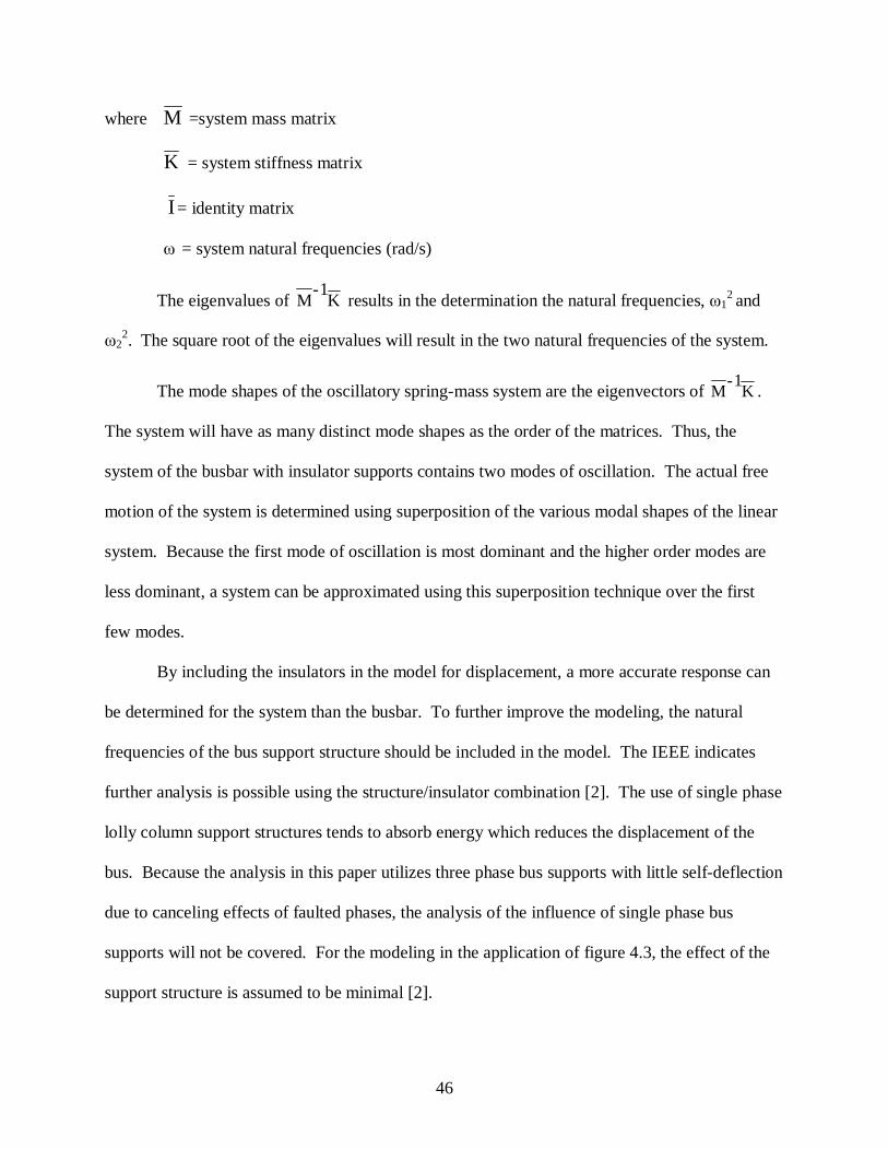
where M =system mass matrix
K = system stiffness matrix
I= identity matrix
= system natural frequencies (rad/s)
The eigenvalues of K1-M results in the determination the natural frequencies, 12 and
22. The square root of the eigenvalues will result in the two natural frequencies of the system.
The mode shapes of the oscillatory spring-mass system are the eigenvectors of K1-M .
The system will have as many distinct mode shapes as the order of the matrices. Thus, the
system of the busbar with insulator supports contains two modes of oscillation. The actual free
motion of the system is determined using superposition of the various modal shapes of the linear
system. Because the first mode of oscillation is most dominant and the higher order modes are
less dominant, a system can be approximated using this superposition technique over the first
few modes.
By including the insulators in the model for displacement, a more accurate response can
be determined for the system than the busbar. To further improve the modeling, the natural
frequencies of the bus support structure should be included in the model. The IEEE indicates
further analysis is possible using the structure/insulator combination [2]. The use of single phase
lolly column support structures tends to absorb energy which reduces the displacement of the
bus. Because the analysis in this paper utilizes three phase bus supports with little self-deflection
due to canceling effects of faulted phases, the analysis of the influence of single phase bus
supports will not be covered. For the modeling in the application of figure 4.3, the effect of the
support structure is assumed to be minimal [2].
Page 58
47
4.3 Dynamic Response of Bundled Conductor Faults
The displacement of bundled conductors during a fault should be equal and opposite as
depicted in figure 4.12 assuming minimal influence from outside phases. This is a characteristic
of the pinch effect discussed in section 3.
d(t) d(t)
i(t)
i(t)/2i(t)/2
i(t)
L
d
Figure 4.12: Bundled Conductor Displacement Due to Fault Forces
Equation 4.17 is an application of equation 3.4 with input current t)sin(ii(t) ω= split
equally between both conductors.
d2t)(sin(i/2)LF
22o
abω
= (4.17)
Figure 4.13 is a plot of equation 4.17 with magnitude of input current equal to 10 kA
RMS, separation distance of 2 ft, and no transient fault current (X/R = 0).
Page 59
48
0 0.005 0.01 0.015 0.02 0.025 0.03 0.035 0.04 0.045 0.050
0.1
0.2
0.3
0.4
0.5
0.6
0.7
Time (s)
Forc
e (#
/in)
Dynamic ForceAverage Force
Figure 4.13:Bundled Conductor Short Circuit Forces
The function is primarily driven by t)(sin2 ω . The sinusoidal function as an input signal
can be broken down into components and its outputs added together via superposition to attain
the system output. The sinusoidal half angle formula [13] can be applied to bundled conductors
to show the components of the linear system.
2)2cos(
21
2t)cos(2-1t)(2sin wt
−==ω
ω (4.18)
Equation 4.18 indicates a DC component equal to half the peak time varying signal. The
AC component is equal to a sinusoidal component with frequency of twice the power frequency.
As discussed throughout section 4, system inputs with frequencies near the system
natural frequencies have the most influence on the output of the system. Equation 4.18 shows
there are two components for the bundled conductor arrangement which can be included as
Page 60
49
inputs to the system. The AC component in a 60 Hz electric system will show up as purely 120
Hz if the X/R ratio is considered negligible. The same holds true after the transient fault current
portions have subsided.
Figure 4.14 shows the influence from the transient portion of fault currents due to the
X/R ratios discussed in section 2. During the presence of the transient component, there is
significant influence from the 60 Hz and DC portions of fault current. The green and red arrows
indicate the development of a 120 Hz sinusoidal function, t)(sin2 ω , in the steady state. The 0,
60, and 120 Hz components are displayed in figure 3.7 via Fourier analysis.
The DC component in the steady state is present for the duration of the fault. The initial
DC component is also present, but varies according to the transient duration. Deflection of the
bus does not vary significantly with varying X/R ratios because the additional DC components
will decay faster than the bus can displace. The amount of DC component in the force signal is
influenced directly by the X/R ratio, as discussed in section 3.
Page 61
50
0 0.02 0.04 0.06 0.08 0.1 0.12 0.14 0.16 0.18 0.20
0.5
1
1.5
2
2.5
Time (s)
Forc
e (#
/in)
DecayingExponentialInfluence
DecayingExponentialInfluence
Steady StateTransient
Figure 4.14: Transient Bundled Conductor Short Circuit Forces
The deflection on a bus span to an input signal must be evaluated during design to ensure
the bus is not excited electrically near the natural frequencies of the bus span. Based on the
research of this paper and [2], it can be concluded that the higher order frequencies of the input
waveform have little influence on the bus span. The approach of using the DC component of the
fault current as the primary and most influential component of the conductor motion can be
utilized effectively, regardless of typical X/R ratios. For the purpose of this paper in its
recommendations for fault detection, the bus span’s natural frequencies should have negligible
influence from the AC component of the fault current forces. It is the DC component which will
Page 62
51
have the most significant impact. The DC component input is the average of the electromagnetic
force generated. An example of this is depicted in figure 4.15.
0 0.02 0.04 0.06 0.08 0.1 0.12 0.14 0.16 0.18 0.20
0.5
1
1.5
2
2.5
Time (s)
Forc
e (#
/in)
Dynamic ForceAverage Force
Figure 4.15: Average Bundled Conductor Short Circuit Forces
Using the average input force as the input function to the dual spring-mass system, the
displacement of the conductor midspan can be accurately modeled. The fundamental frequency
becomes the most important setting for the conductor response to this input function. It
primarily drives conductor deflection generally slower than the transient component of fault
current can influence deflection. This simplifies analysis of bundled conductor deflection by
using the input function of the average input force.
Page 63
52
5.0 Optical Method of Fault Detection
Electromechanical forces generated during power system faults affect all power system
equipment in series with the fault. This includes insulators, conductors, support structures,
breakers, transformers, and generators. Theoretically, any of these power system components
could be measured for the effects of fault current detection. For example, stresses on insulators
or structures could be measured using strain gauges. This paper focuses on the optical method of
detection in which the motion of the conductor span is measured at its midpoint. The span can
then be designed to provide accurate detection which can be integrated into a relay time-
overcurrent curve.
5.1 Physical Configuration
Conventional relay selection and settings require the use of set points to trigger action
upon detection of faults. The conductor dynamics approach to fault detection also requires set
points. The method for choosing a single set point will be discussed in this section. This set
point is the determined using the physical analysis of conductor deflection and integrating to the
electrical domain of relay settings.
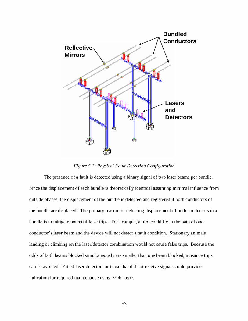
Crucial to understanding the operation of the optical fault detection system is the
proposed physical configuration of figure 5.1. Each conductor is equipped with a reflective
mirror which reflects normal to the ground plane. Its purpose is to reflect a transmitted laser
source back to its detector located beneath each mirror.
Page 64
53
ReflectiveMirrors
LasersandDetectors
BundledConductors
Figure 5.1: Physical Fault Detection Configuration
The presence of a fault is detected using a binary signal of two laser beams per bundle.
Since the displacement of each bundle is theoretically identical assuming minimal influence from
outside phases, the displacement of the bundle is detected and registered if both conductors of
the bundle are displaced. The primary reason for detecting displacement of both conductors in a
bundle is to mitigate potential false trips. For example, a bird could fly in the path of one
conductor’s laser beam and the device will not detect a fault condition. Stationary animals
landing or climbing on the laser/detector combination would not cause false trips. Because the
odds of both beams blocked simultaneously are smaller than one beam blocked, nuisance trips
can be avoided. Failed laser detectors or those that did not receive signals could provide
indication for required maintenance using XOR logic.
Page 65
54
The entire fault detection span should be housed inside an electrical substation. The
equipment used requires power, control, and signal cables. It should ideally be near its
interrupting device for quick response. Additionally, such a bus span can easily be integrated
into line and transformer bays if consideration is given for the required span distance. Finally,
interference from the public should be minimized inside the gates of the substation. For these
reasons, installation of such a bus span is ideal inside a substation.
5.2 Time-Current Coordination
A fault occurring anywhere in series with a protective device should be detected provided
sufficient fault current flows to displace the bus past its at rest reflective mirror location. As is
the nature of fault currents, the further away from the source, the more line impedance limits the
magnitude of fault current. Consideration should be given based on system topology and
possible fault locations to determine set points. The same logic applies for conventional
transmission line relaying settings.
In the event of a fault, all three phases are generally tripped. The type of fault and phases
involved are irrelevant if the logic is designed to trip all three phases. Thus, the detection and
settings must hold to the weakest and least detectable fault scenario. The system topology must
be accurately modeled and analyzed to determine if it will trip for all types of fault scenarios.
Figure 5.2 depicts an electrical representation of the trip logic using AND and OR gates with the
phasing convention of figure 3.11.
Page 66
55
Timer Trip
Figure 5.2: Electrical Diagram of Detection Logic
The inverted phase detector signal is used as inputs to the logic diagram. If the mirror
reflects from the source to the detector, the input signal used is represented as a 0 in the diagram.
If the bus is displaced beyond the mirror such that it does not reflect back, the input of a 1 is used
in the logic diagram.
The OR gate is used to send an instantaneous displacement signal on any set of bundled
conductors to the timer. The timer should be set according to system topology. It is the set point
for the system and is based on the amount of time the bus has been displaced from its natural
form of a straight physical beam.
The size of the reflective mirror is important in determining the timer setting. Any bus
deflection which is smaller than the mirror size does not trigger a displacement signal. This
allows for some flexibility in alignment tolerances as well as vibrations due to mild seismic or
low wind conditions. Static influence of wind on the bus response is briefly discussed in [2] and
can be analyzed in the design process if required. Alternately, the system could be disabled if
gusts are detected. Unfortunately, this may work against the purpose of the system. Line faults
Page 67
56
are often triggered by trees brushing in the wind against conductors. Disabling the system for
such a gust could prove disastrous for power system equipment in series with the faulted line.
Figure 5.3 illustrates a profile view of figure 5.1. The importance of the mirror size is
emphasized. Ideally, the system should focus the beam at the center of the mirror. During
deflection, the beam should clear the mirror without reflecting. Such is the basis for the binary
operation if the bus has deflected due to fault current forces.
NeutralPosition Deflected
Position
Beam
Mirror
Laser andDetector
Figure 5.3: Profile View of Physical Fault Detection Configuration
Figure 5.4 shows an example of conductor displacement due to fault current forces. The
red line is determined by the size of the reflective mirror. If the displacement is greater than ½
of the mirror length, the reflection does not occur and bus displacement is recognized (figure 5.5)
as a binary signal.
Page 68
57
-10
-5
0
5
10
15
20
0.00
0.13
1.01
1.13
1.74
2.57
3.42
4.35
4.94
5.01
5.10
5.82
6.59
7.44
8.34
9.14
9.98
Time (s)
Disp
lace
men
t (in
)
1/2 Lmirror
Figure 5.4: Conductor Displacement with Reflecting Mirror Position
0
1
0.00
0.13
1.01
1.13
1.74
2.57
3.42
4.35
4.94
5.01
5.10
5.82
6.59
7.44
8.34
9.14
9.98
Time (s)
Bina
ry D
efle
ctio
n St
atus
Pulse #1 Width Pulse #2 Width
Figure 5.5: Deflection Displacement Detection Pulses
Page 69
58
The two pulses shown in figure 5.5 are a result of displacement beyond that of the
reflecting mirror width. Proper setting of a delay timer causes the logic diagram of figure 5.2 to
ignore pulse #2. The trip signal should not be initiated based on the oscillation of the bus after
the fault is cleared. Pulse #1 is a large amount of time and the setting of the delay timer should
trigger a trip signal for such a length of time.
Inspection of figure 5.4 shows that the size of the mirror does have considerable impact
on the detection pulses of figure 5.5. If the mirror size was chosen to be larger than 5, the second
pulse would not exist in the detection plot of figure 5.5. If the mirror was chosen to be less than
5”, more secondary pulses would be present in the detection plots. The delay timer would need
to be adjusted not to trip on these additional pulses.
When the fault current forces are relieved due to interrupting devices, the bus returns to
its at rest position. The amount of time required for this to occur is a function of the fundamental
frequency of the conductor span.
Figure 5.6 shows this dependence upon the natural frequency. T1 is the time in which the
fault current is cleared. T2 is the time at which the pulse signal is detected.
Page 70
59
-8
-6
-4
-2
0
2
4
6
8
10
12
4.58
4.93
5.00
5.01
5.04
5.15
5.57
6.02
6.47
6.95
7.44
7.92
8.45
8.92
9.39
9.87
Time (s)
Dis
plac
emen
t (in
) 1/2Lmirror
T1 T2
Figure 5.6: Conductor Displacement Following Fault Clearing
The time period of conductor motion from its deflected position to the at rest position
follows that of equation 5.1.
t)cos(T1T2 n=− (5.1)
The fall time indicated as T2-T1 should be considered in selection of conductor natural
frequency and time delay settings. Timer settings and mirror sizing should be determined based
on this fall time. To minimize unnecessary outages, the amount of time required for the bus to
return to its at rest position should be reflected in the timer setting and mirror size.
The pulse width is the primary means of fault detection. The time delay setting of the
relay should be set as the threshold for the trip signal. The setting should be designed to not send
a trip signal until any primary relaying has a chance to operate. This also applies to relaying
Page 71
60
associated with circuit breakers closer to the faulted segment. Deflection of the bus for these
occurrences must be calculated to ensure proper relay settings.
0.01
0.1
1
10
100
1000
1 10 100 1000 10000 100000Current (A)
Tim
e (s
)
Primary Relay Damage CurveBus Dynamic FaultDetector Relay
Figure 5.7: Typical Bus Dynamic Fault Detector Setting
The fault detector based on conductor dynamics cannot retrieve fault current data
directly. The use of the pulse width is the only means of detecting the fault. This is plotted as a
single line on the time-overcurrent curve. The red line of figure 5.7 does not reach the X axis
because it has a delay of approximately 0.2 seconds before detection is possible. This is based
on the fundamental frequency of the bus span. It is important for the setting to be before the
equipment damage curve, but not act before the primary relay has acted.
The logic described in figure 5.2 must produce a trip signal for any type of conductor
fault. The relay timer setting to be calibrated using the smallest type of fault current desired. For
faults near the detector, this could be slightly less than the maximum calculated fault current;
Page 72
61
however, this approach is not recommended since it is reflective of a bolted fault. If any
impedance is inserted in a fault or if a fault occurs down a segment of line, the delay setting may
not detect due to a limited deflection. Thus, the fault would be undetected.
The fault current for different types of faults will vary. As discussed in section 2, these
differ according to system topology. The settings used for the fault detector should reflect the
smallest of the types of fault currents. The use of bundled conductors with proper spacing will
minimize the displacement due to outside phases, so the smallest value of fault current for the
various types of faults should be considered for this reason. The span response must also be
analyzed for larger fault currents to ensure conductor stresses are not violated or collisions inside
bundles do not occur.
d1(t) d1(t) d2(t) d2(t) d3(t) d3(t)
Aø Dø Bø Eø Cø Fø
i1(t) i2(t) i3(t)
Figure 5.8: Displacement of Conductor Bundles
Figure 5.8 shows the deflection resulting from different fault currents to the power
system. Realization that the deflection from bundle to bundle will differ according to type of
fault is crucial in the design phase.
Page 73
62
5.3 Multiple Circuit Detection Coordination
Coordination of fault detection using multiple circuits inside a substation can be
accomplished by setting the relays for the appropriate amount of fault current for each circuit.
Each fault scenario should be analyzed to determine what the minimum time delay setting or
mirror size should be for each fault detector. The value of fault current through a circuit will
vary according to contribution based on faulted circuit location and selection. This variance
should be analyzed to determine maximum and minimum fault current levels for a particular
circuit. This information is necessary to properly set the timer of the protection device.
Figure 5.9 shows a 4 circuit substation bus with a fault on circuit 1. Fault current
contributions from circuits 2, 3, and 4 are indicated as 5kA, 10kA, and 12kA respectively.
CB3 CB4CB1 CB2
Substation Bus
Circuit 2Circuit 1 Circuit 4Circuit 3
5kA 10kA 12kA
27kA
FaultDetector
Figure 5.9: Fault Current Contributions for Fault on Circuit 1
Figures 5.10 through 5.12 show the scenarios of faults on circuits 2, 3, and 4 for the same
substation bus as figure 5.9.
Page 74
63
CB3 CB4CB1 CB2
Substation Bus
Circuit 2Circuit 1 Circuit 4Circuit 3
7kA 10kA 12kA
29kA
Figure 5.10: Fault Current Contributions for Fault on Circuit 2
CB3 CB4CB1 CB2
Substation Bus
Circuit 2Circuit 1 Circuit 4Circuit 3
7kA 12kA
24kA
5kA
Figure 5.11: Fault Current Contributions for Fault on Circuit 3
Page 75
64
CB3 CB4CB1 CB2
Substation Bus
Circuit 2Circuit 1 Circuit 4Circuit 3
7kA
22kA
5kA 10kA
Figure 5.12: Fault Current Contributions for Fault on Circuit 4
Table 5.1 shows a summary of figures 5.9 through 5.12. Inspection of this table shows
circuit 1 should not provide a trip signal for 7kA, but should for 27kA. The timer setting should
be adjusted to compensate for this. Appropriate timer delay settings can be calculated using the
methodology presented in section 5.2. The values for circuits 2, 3, and 4 can be determined from
the table as well.
Table 5.1: Fault Current Contributions for Various Faulted Circuits
Faulted Circuit Circuit 1 Current Circuit 2 Current Circuit 3 Current Circuit 4 Current1 27kA 5kA 10kA 12kA2 7kA 29kA 10kA 12kA3 7kA 5kA 24kA 12kA4 7kA 5kA 10kA 22kA
It is recommended that every fault situation be analyzed in a table similar to table 5.1.
This allows for recognition of fault current levels for determination of relay settings. While such
analysis is not necessary for every application, its need should be evaluated in the design of the
conductor dynamic fault detection system.
Page 76
65
6.0 Conclusions and Further Research
The use of conductor dynamics in detecting faults is not a common practice in the electric
grid. Modern protection practices commonly utilize current and potential transformers to
measure currents and voltages. Detection based on conductor deflection adds a different form of
protection which could prove valuable in the event of relay, current transformer, and potential
transformer failures. Conductor response to electromagnetic forces during fault conditions is a
physical phenomenon which can be monitored for fault detection.
The focus of the research presented is on the optical means of fault detection for the large
power system inside substations. The use of bundled rigid conductors has several distinct
advantages over single conductor applications. These include conductor displacement for single
phase faults equal in magnitude to polyphase faults. False trips due to beam blockage can be
minimized by triggering on symmetric motion inside a bundle. Additionally, triggering of
conductor motion regardless of load current on unfaulted phases is attainable.
Fortunately, the electromagnetic forces generated during fault conditions extend to a
variety of applications. The tools presented in the paper should allow a power system designer
to effectively analyze and design substation conductor spans for the purpose of fault detection.
The concept of fault detection using conductor dynamics is not impractical. Through
detailed analysis of substation rigid bus, this paper demonstrates the feasibility of this
application.
Page 77
66
6.1 Suggestions for Further Research
While the mathematical approach to fault detection is discussed in detail throughout this
paper, it is beneficial to verify the actual conductor motion for a span using test equipment. The
use of a power laboratory for the purpose of verification and calibration was unavailable during
the time of this research. One suggestion for further research is conductor displacement
verification for a variety of conductor spans and fault durations using bundled conductors in a
laboratory setting.
The analysis of the substation bus spans was accomplished using dynamic analysis
similar to a dual spring-mass system. This gives a true representation of forces and response as a
function of time. Because bundled rigid conductors are not commonly used or analyzed in
substation bus designs, a second suggestion for further research is the application of finite
element analysis techniques [4, 5]. Comparisons of finite element analysis to measured results
for single conductor arrangements have proved to be more accurate than dynamic analysis [4].
Page 78
67
Appendix A
Design Application of Fault Detection using
Conductor Dynamics
The objective of appendix A is to design and provide settings for a backup relay for the
transmission line of the power system in the electrical oneline of figure A.1. The detector should
operate in 60 cycles (1 second) if the primary relaying fails.
Load #1 Load #2
CB
1
21
51
Proposed Locationof Fault Detector
Transmission Line
Substation A Substation B
Gen #1
Figure A.1.: Appendix A Power System Electrical Oneline
Buses 1 and 2 are energized at 230kV with circuit breaker CB1 rated at 1200 amps RMS
and interrupting capability of 40kA RMS. One overcurrent relay (type 51) with current
transformers is used to trip for faults on the transmission line connecting buses 1 and 2.
The proposed location of the fault detector using bus dynamics is shown in red. It is in
series with the transmission line to be protected. It is placed ahead of the circuit breaker;
however, electrically it could be placed behind it. In order to properly coordinate with the
overcurrent relay, it should monitor the same line and thus be in series.
Page 79
68
Table A.1 shows the calculated fault current values at buses 1 and 2 with and without a
40 ohm fault impedance. The X/R ratios at each bus are also given. This data was calculated
using system topology and is considered a required input for design of the fault detector.
Table A.1.Appendix A RMS Fault Current Values
Bus 1 Bus 2Bolted FaultPhase - Ground 38.5kA 36.5kAPhase – Phase 39kA 37kAPhase - Phase - Ground 39kA 37kAThree Phase 40kA 40kA
40 Ohm ImpedanceFaultPhase - Ground 32kA 30kAPhase – Phase 32.5kA 30.5kAPhase - Phase - Ground 32.5kA 30.5kAThree Phase 33 kA 31kA
X/R Ratio 15 15.67
The detector using bus dynamics will be constructed as shown in figure 5.1. Bundled
rigid bus will be utilized for the advantages discussed previously. Several design parameters
need to be established including conductor type, separation distances, span length, and conductor
settings.
The first parameter to establish is the minimum conductor size according to ampacity. If
the bus span is chosen to match the ampacity of the breaker size, each phase of the conductor
bundle should be rated 600 amps assuming maximum load current splitting equally in the
bundle. According to [2], any schedule 40 tubular aluminum 6061-T6 bus greater than 1”
diameter will suffice for ampacity purposes. A 2-1/2” tubular bus has been chosen for this
application to raise the natural frequency of the span and thus increase the response time.
Figures A.2 and A.3 show the phase to ground fault current including transient
components from the system X/R ratio. The plots were developed from the given system fault
Page 80
69
information and the use of equations 2.9 and 2.10. The 40 ohm fault impedance values were
chosen because they represent a relatively low fault value compared to a less common and higher
bolted fault. Assuming the fault detector can operate for the fault with impedance, the bolted
fault detector should also work for a bolted fault. The load current of 1200 amps RMS on the
unfaulted phases is also shown for comparative purposes.
According to the given fault data in table A.1, the smallest value of fault current is at bus
#2 with an X/R ratio of 15 and a 40 ohm impedance fault. This will be analyzed for setting
configuration.
0 0.02 0.04 0.06 0.08 0.1 0.12 0.14 0.16 0.18 0.2-6
-4
-2
0
2
4
6
8x 10
4
Time (s)
Cur
rent
(Am
ps)
IaIbIc
Figure A.2.: Phase to Ground Fault Current
Page 81
70
0 0.02 0.04 0.06 0.08 0.1 0.12 0.14 0.16 0.18 0.2-5
0
5
10x 10
4
Time (s)
Cur
rent
(Am
ps)
IaIbIc
Figure A.3.: Three Phase Fault Current
The selection of conductor bundle and phase spacing can be narrowed down according to
available space inside the substation and typical conductor arrangements. In this example, the
arrangement of figure 3.11 will be used with d = 2 ft and S = 12 ft. The length of the span and
conductor type will be chosen after the forces have been calculated.
The electromagnetic forces can be calculated for each conductor using equation 3.4.
These forces are vectorially added according to equations 3.8 through 3.13. The results are
presented in figures A.4 through A.9. The direction of force is seen as symmetric about the X
axis. This physically is seen as the pinching of the conductors in a bundle towards each other.
Page 82
71
0 0.02 0.04 0.06 0.08 0.1 0.12 0.14 0.16 0.18-5
-4
-3
-2
-1
0
1
2
3
4
5
Time (s)
Forc
e (#
/in)
FaFdFbFeFcFf
Figure A.4: A Phase to Ground Fault Conductor Forces
0 0.02 0.04 0.06 0.08 0.1 0.12 0.14 0.16 0.18-6
-4
-2
0
2
4
6
Time (s)
Forc
e (#
/in)
FaFdFbFeFcFf
Figure A.5: A to B Phase Fault Conductor Forces
Page 83
72
0 0.02 0.04 0.06 0.08 0.1 0.12 0.14 0.16 0.18-6
-4
-2
0
2
4
6
Time (s)
Forc
e (#
/in)
FaFdFbFeFcFf
Figure A.6: A to B Phase to Ground Fault Conductor Forces
0 0.02 0.04 0.06 0.08 0.1 0.12 0.14 0.16 0.18-6
-4
-2
0
2
4
6
Time (s)
Forc
e (#
/in)
FaFdFbFeFcFf
Figure A.7: A to C Phase Fault Conductor Forces
Page 84
73
0 0.02 0.04 0.06 0.08 0.1 0.12 0.14 0.16 0.18-6
-4
-2
0
2
4
6
Time (s)
Forc
e (#
/in)
FaFdFbFeFcFf
Figure A.8: A to C to Ground Phase Fault Conductor Forces
0 0.02 0.04 0.06 0.08 0.1 0.12 0.14 0.16 0.18-8
-6
-4
-2
0
2
4
6
Time (s)
Forc
e (#
/in)
FaFdFbFeFcFf
Figure A.9: Three Phase Phase Fault Conductor Forces
Page 85
74
The force plots indicate a waveform similar to figure 4.14. The use of bundled
conductors shows near symmetry for bundles and thus depicts near equal force distribution
between conductor bundles. While there is some notable interaction between faulted conductor
phases outside the bundles, the settings can be determined based on the deflection of any bundle
involved in the fault. In other words, there are some notable differences on the three phase plot
of figure A.5; however, the settings can be designed to detect the largest deflection. The settings
chosen should also allow for any deflection differences within bundles due to forces from outside
phases at any moment in time.
The forces due to unfaulted phases appear negligible in comparison with the faulted ones.
This is due to the ratio of fault to load current and the large separation distances in equation 3.4.
The result is negligible deflection due to load currents.
The plots for B phase to ground and C phase to ground forces were not shown because
they are the same as figure A.4 with the exception of the bundled conductor generating
electromagnetic forces. The same holds true for the B to C phase and B to C phase to ground
faults.
The insulators required for the bus span assembly were 230kV voltage class station post
insulators. The mechanical specifications [5] for the insulators are contained in table A.2.
Table A.2.NGK 8A-67971A 230kV Insulator Mechanical Specifications
Insulator Description QuantityHeight 80 inCore Diameter 5 inMax Cantilever Load 2810 lbSpring Constant 2631 lb/inWeight 322 lbPoisson's Ratio 0.3
Page 86
75
The spring constant for the conductor span is determined using equation 4.7. Using fixed
ends on the span with 2-1/2” schedule 40 aluminum 6061-T6 conductor, the value of kbus is
calculated to be 25508.35 lb/in.
The mass matrix of equation 4.14 is built assuming m1 is the effective weight of the
conductor transmitted to the support fitting. This translates to ½ the weight of the conductor.
The full weight of the conductor is m2. Since the conductor’s weight is given as 2.004 lb/ft, the
20 foot span design would create a system mass matrix:
=
08.400004.20
M
The system stiffness matrix is determined to be:
−
−=
35.2550835.2550835.2550835.28139
K
Determination of the natural frequencies for a system is accomplished using equation
4.16. The eigenvalues of K1-M are solved using computer software to provide two solutions,
21 and 2
2 . The natural frequencies are calculated to be 44.1233 rad/s (7.0260 Hz) and 9.5745
rad/s (1.5246 Hz). Thus, the fundamental frequency is 1.5246 Hz.
Because of the low natural frequencies, the DC component of the fault short circuit forces
can be approximated using the system step response. The magnification factor for the 120Hz
steady state fault current is calculated using equation 4.5 to be 6% gain for the AC portion. To
ensure this is recognized through modeling, a margin will be applied to the minimum pulse
width.
The primary relay settings are given in figure A.10. A backup relay for the system
should take the form of a vertical line on the overcurrent relay setting plot (figure 1.3).
Page 87
76
0.01
0.1
1
10
100
1000
1 10 100 1000 10000 100000Current (A)
Tim
e (s
)Primary Relay Backup Relay
Figure A.10: Primary Overcurrent Relay Settings
The physical response of the bundled conductors to a three phase fault at bus #2 is
depicted in figure A.11 at time t=1sec. The response assumes the primary relay has tripped at
0.07 seconds. This is equivalent to a step function to the bus system for duration of 0.07 seconds
(including breaker operation with detection according to figure A.10).
The reflecting mirrors for all phases will be 5”. This could be adjusted if necessary for
lower magnitude faults. Figure A.11 shows the mirror size as ½ Lmirror equal to 2 ½”.
Figure A.12 shows the pulse width produced representing deflection during operation of
the primary relaying. The pulse width is .067 seconds. It is critical, therefore, for the setting of
the fault detector to be above this value. Since this reflects a 30kA fault, the pulse width for a
Page 88
77
40kA fault (maximum) is also calculated to be .080 seconds. For a margin of protection, the
value of 0.1 second pulse width will be considered as the minimum pickup pulse width.
-2
-1.5
-1
-0.5
0
0.5
1
1.5
2
2.5
3
0
0.42 1
1.08
1.22
1.37
1.51
1.63
1.79
1.95
2.12 2.
3
2.5
2.77
3.07 3.
4
Time (s)
Dis
plac
emen
t (in
) 1/2 Lmirror
Figure A.11: Conductor Deflection Using Primary Relaying
0
1
0
0.34 1
1.07
1.17 1.3
1.45
1.54
1.67
1.82
1.99
2.14 2.3
2.48
2.73
2.97
3.24
3.77
Time (s)
Bina
ry D
efle
ctio
n St
atus
Pulse Width
Figure A.12: Pulse Width Using Primary Relaying
Page 89
78
The next step in determining the relay settings is calculation of conductor displacement
during each type of fault in figures A.4 through A.8. Figures A.13 through A.28 show the
displacement for the faulted bundles and the associated pulse widths using a mirror size of 5”.
Table A.3 lists the displacement detector’s time for each conductor bundle using the fault
conditions in figures A.4 through A.9.
Table A.3: Detection Time Table Summary
Fault TypeA Phase to Ground 0.88s 0.88s - - - -A to B Phase 0.783s .903s .903s .783s - -A to B Phase to Ground .808s .903s .903s .808s - -A to C Phase .808s .903s - - .903s .808sA to C Phase to Ground .888s .903s - - .903s .888sThree Phase .805s .903s .903s .903s .903s .803s
Min. Bundle Overlap Time .777s .783s .732s
It can be determined from figures A.13 through A.28 and table A.3 that the minimum
detection time for the 30kA fault is a three phase fault on the outer conductor bundles. The time
for the mutual displacement is 0.732 seconds assuming the fault is cleared by opening the circuit
breaker after 1 second (60 cycles). It can then be concluded that the required delay time for the
logic diagram of figure 5.2 should be 0.73 seconds for a 30kA fault or above. If less than a 1
second time is desired, the analysis can be rerun to determine the new setting. Additionally, if
the fault current is higher than 30kA, the device will still operate. The time-overcurrent setting
curve of the device is represented as the red line of figure A.10.
Page 90
79
-4
-2
0
2
4
6
8
0
0.43
1.01
1.16
1.37
1.77
2.05
2.19
2.33
2.51 2.
7
2.92
3.08
3.44 4.
2
4.98
Time (s)
Dis
plac
emen
t (in
)
A phaseD phase
1/2 Lmirror
Figure A.13: A Phase to Ground Fault Conductor Displacements
0
1
0
0.33
1.01
1.11 1.3
1.53 2
2.1
2.23
2.36
2.53 2.7
2.91
3.02
3.32 3.9
4.62
Time (s)
Bina
ry D
efle
ctio
n St
atus
A PhaseD Phase
0.88 sec
Figure A.14: A Phase to Ground Fault Conductor Deflection Detector Pulses
Page 91
80
-4
-2
0
2
4
6
8
10
12
0
0.33
1.01
1.11 1.
3
1.53 2
2.1
2.23
2.36
2.53 2.
7
2.91
3.02
3.32 3.
9
4.62
Time (s)
Dis
plac
emen
t (in
)
A phaseD phase
1/2 Lmirror
Figure A.15: A to B Phase to Phase Fault Conductor Displacements
0
1
0
0.33
1.01
1.11 1.3
1.53 2
2.1
2.23
2.36
2.53 2.7
2.91
3.02
3.32 3.9
4.62
Time (s)
Bina
ry D
efle
ctio
n St
atus
A PhaseD Phase
0.903 sec
0.783 sec
Figure A.16: A to B Phase to Phase Fault Deflection Detector Pulses
Page 92
81
-4
-2
0
2
4
6
8
10
0
0.33
1.01
1.11 1.
3
1.53 2
2.1
2.23
2.36
2.53 2.
7
2.91
3.02
3.32 3.
9
4.62
Time (s)
Dis
plac
emen
t (in
)
A phaseD phase
1/2 Lmirror
Figure A.17: A to B Phase to Ground Fault Conductor Displacements
0
1
0
0.33
1.01
1.11 1.3
1.53 2
2.1
2.23
2.36
2.53 2.7
2.91
3.02
3.32 3.9
4.62
Time (s)
Bina
ry D
efle
ctio
n St
atus
A PhaseD Phase
0.903 sec
0.808 sec
Figure A.18: A to B Phase to Ground Fault Deflection Detector Pulses
Page 93
82
-4
-2
0
2
4
6
8
10
0
0.33
1.01
1.11 1.
3
1.53 2
2.1
2.23
2.36
2.53 2.
7
2.91
3.02
3.32 3.
9
4.62
Time (s)
Dis
plac
emen
t (in
)
A phaseD phase
1/2 Lmirror
Figure A.19: A to C Phase to Phase Fault Conductor Displacements
0
1
0
0.33
1.01
1.11 1.3
1.53 2
2.1
2.23
2.36
2.53 2.7
2.91
3.02
3.32 3.9
4.62
Time (s)
Bina
ry D
efle
ctio
n St
atus
A PhaseD Phase
0.903 sec
0.808 sec
Figure A.20: A to C Phase to Phase Fault Deflection Detector Pulses
Page 94
83
-4
-2
0
2
4
6
8
10
0
0.33
1.01
1.11 1.
3
1.53 2
2.1
2.23
2.36
2.53 2.
7
2.91
3.02
3.32 3.
9
4.62
Time (s)
Dis
plac
emen
t (in
)
A phaseD phase
1/2 Lmirror
Figure A.21: A to C Phase to Ground Fault Conductor Displacements
0
1
0
0.33
1.01
1.11 1.3
1.53 2
2.1
2.23
2.36
2.53 2.7
2.91
3.02
3.32 3.9
4.62
Time (s)
Bin
ary
Def
lect
ion
Sta
tus A Phase
D Phase
0.903 sec
0.888 sec
Figure A.22: A to C Phase to Ground Fault Deflection Detector Pulses
Page 95
84
-4
-2
0
2
4
6
8
10
0
0.33
1.01
1.11 1.
3
1.53 2
2.1
2.23
2.36
2.53 2.
7
2.91
3.02
3.32 3.
9
4.62
Time (s)
Dis
plac
emen
t (in
) A phaseD phase1/2 Lmirror
Figure A.23: Three Phase Fault A and D Bundle Conductor Displacements
0
1
0
0.33
1.01
1.11 1.3
1.53 2
2.1
2.23
2.36
2.53 2.7
2.91
3.02
3.32 3.9
4.62
Time (s)
Bina
ry D
efle
ctio
n S
tatu
s A PhaseD Phase
0.903 sec
0.805 sec
0.777 secoverlap
Figure A.24: Three Phase Fault A and D Bundle Deflection Detector Pulses
Page 96
85
-4
-2
0
2
4
6
8
10
0
0.33
1.01
1.11 1.
3
1.53 2
2.1
2.23
2.36
2.53 2.
7
2.91
3.02
3.32 3.
9
4.62
Time (s)
Dis
plac
emen
t (in
) B PhaseE Phase1/2 Lmirror
Figure A.25: Three Phase Fault B and E Bundle Conductor Displacements
0
1
0
0.33
1.01
1.11 1.3
1.53 2
2.1
2.23
2.36
2.53 2.7
2.91
3.02
3.32 3.9
4.62
Time (s)
Bin
ary
Defle
ctio
n St
atus
B PhaseE Phase
0.903 sec
Figure A.26: Three Phase Fault B and E Bundle Deflection Detector Pulses
Page 97
86
-4
-2
0
2
4
6
8
10
0
0.33
1.01
1.11 1.
3
1.53 2
2.1
2.23
2.36
2.53 2.
7
2.91
3.02
3.32 3.
9
4.62
Time (s)
Dis
plac
emen
t (in
) C PhaseF Phase1/2 Lmirror
Figure A.27: Three Phase Fault C and F Bundle Conductor Displacements
0
1
0
0.33
1.01
1.11 1.3
1.53 2
2.1
2.23
2.36
2.53 2.7
2.91
3.02
3.32 3.9
4.62
Time (s)
Bin
ary
Defle
ctio
n St
atus
C PhaseF Phase
0.903 sec
0.803 sec
0.732 secoverlap
Figure A.28: Three Phase Fault C and F Bundle Deflection Detector Pulses
Page 98
87
Appendix B
Bus Dynamic Fault Detector Design Flowchart
Set span length,mirror size, bundle
separation
Attain SystemFault Data
DetermineOptimal Detector
Location
Choose MinimumConductor Size
(Ampacity)
Determinemaximum forces
Do forcesexceed span
stresses?
Yes
NoCalculate NaturalFrequencies
Are frequenciesnear drivingfrequencies?
YesNo
CalculateConductor
Displacements
Aredisplacementsadequate fordetection?
No
Yes Done
Figure B.1: Design Flowchart
Page 99
88
References
[1] Grainger, John J. & Stevenson, William D. Jr, “Power System Analysis,” McGraw-
Hill, Inc., 1994.
[2] Substations Committee of the IEEE Power Engineering Society, “IEEE Guide for
Design of Rigid-Bus Structures,” IEEE Std 605-1998, August 1998.
[3] Meliopoulos, A.P. Sakis, “Power System Grounding and Transients: An
Introduction,” Marcel Dekker, Inc., 1988.
[4] Develle, B.A., “Finite Element Analysis Applied to Substation Busbar Design,”
Graduate Thesis, University of New Orleans, May 1992.
[5] Bergeron, David Allen, “Improved Static Finite Element Analysis of Substation
Busbar Structures,” Graduate Thesis, University of New Orleans, December 1995.
[6] Ward, Daniel J, “Overhead Distribution Conductor Motion Due to Short-Circuit
Forces”, IEEE Transactions on Power Delivery, Vol. 18, No. 4, October, 2003.
[7] Halliday, David; Resnick, Robert; Walker, Jearl, “Fundamentals of Physics, Fourth
Edition”, John Wiley & Sons, Inc, 1993.
[8] American Institute of Steel Construction, “Manual of Steel Construction”, July, 1989
[9] Thomson, William T & Dahleh, Marie Dillon, “Theory of Vibration with
Applications, Fifth Edition,” Prentice-Hall, Inc., 1998, 1993.
[10] Beer, Ferdinand P. & Johnston, Russell E. Jr, “Vector Mechanics for Engineers:
Dynamics, Sixth Edition”, The McGraw-Hill Companies, Inc., 1997.
[11] Landry, Michel; Beauchemin, Roger; Venne, Andre, “De-icing EHV Overhead
Transmission Lines Using Electromagnetic Forces Generated by Moderate Short-
Circuit Currents” IEEE Transactions on Power Delivery, 37C-TP-15, 2000.
Page 100
89
[12] Chen, Huaxiong, “System Identification Applications in Substation Busbar
Structure Modeling”, Graduate Thesis, University of New Orleans, July 1996.
[13] Stewart, James, “Calculus: Early Transcendentals, Third Edition”, Brooks/Cole
Publishing Company, 1995
Page 101
90
Vita
Jeff Dicharry was born in New Orleans, LA in 1978. He attended Brother Martin
High School and graduated with a Bachelor’s Degree in Electrical Engineering from
Louisiana State University in December, 2000. He was employed in the substation
design group of Entergy Services, Inc. from January, 2001 to November, 2004. He is
involved with the rigid bus and cable systems subcommittees of the IEEE substation
committee with contributions including conductor ampacity calculations. He is currently
employed in the Transmission Operations Planning group of Entergy Services, Inc. and is
completing his Master of Science in Electrical Engineering from the University of New
Orleans. He hopes to continue working in the power industry and utilize his employment
and educational experiences to teach collegiate level engineering courses in the future.