POWER SYSTEMS & SIMULATION LABORATORYcrectirupati.com/sites/default/files/lab1/PS&S LAB IV-I.pdf5...

LABORATORY MANUAL

ON

POWER SYSTEMS & SIMULATION

LABORATORY

2018 – 2019

IV B. Tech I Semester (JNTUA-R15)

Mr. Kondragunta Jagadish Babu, Assistant Professor

CHADALAWADA RAMANAMMA ENGINEERING COLLEGE (AUTONOMOUS)

Chadalawada Nagar, Renigunta Road, Tirupati – 517 506

Department of Electrical and Electronics Engineering

3

Department of Electrical and Electronics Engineering

LIST OF EXPERIMENTS

1. Determination of sequence impedances of cylindrical Rotor synchronous machine

2. Fault Analysis-I (LG FAULT , LL FAULT)

3. Fault Analysis-II (LLG FAULT , LLLG FAULT)

4. Determination of Subtransient reactances of a salient pole synchronous machine

5. Equivalent circuit of a 3-Ф three winding transformer

6. Gauss-Seidal load flow analysis using MATLAB

7. Fast decoupled load flow analysis using MATLAB

8. Y bus formation using MATLAB

9. Z bus formation using MATLAB

10. Develop a Simulink model for a single area load frequency control problem

11. Newton Raphson Method of load flow analysis using MATLAB

12. Short circuit analysis for line to ground fault and line to line fault using MATLAB

4

EXP.NO: DATE:

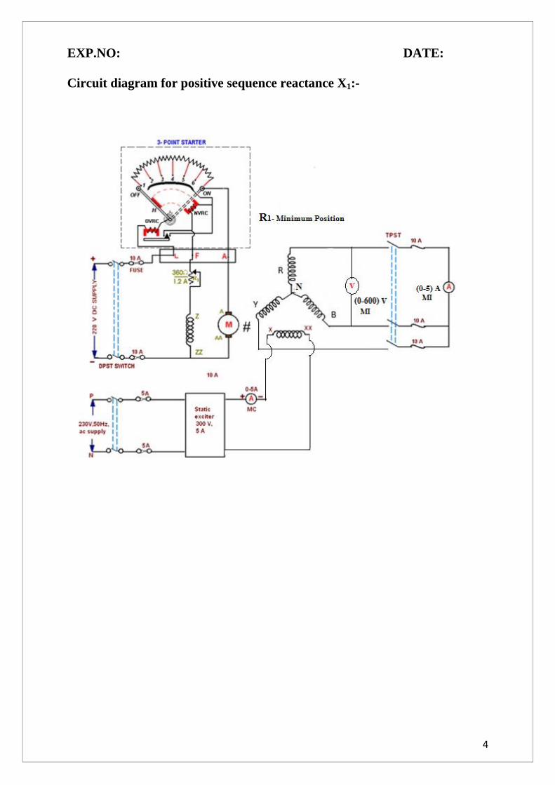
Circuit diagram for positive sequence reactance X1:-

5

EXP.NO: DATE:

1. DETERMINATION OF SEQUENCE IMPEDANCES OF

CYLINDRICAL ROTOR SYNCHRONOUS MACHINE

Aim:-To determine experimentally Positive, Negative and Zero sequence reactance’s of a

cylindrical rotor synchronous machine.

Name Plate Details:-

S.No Parameter Alternator DC Motor

1 Rated Voltage 415 V 220 V

2 Rated Current 4.2 A 20 A

3 Speed 1500 RPM 1500 RPM

4 Rating 3 KVA 5 HP

5 Power factor 0.8 -----

6 Frequency 50 Hz -----

7 Excitation 220 V, 2 A

Apparatus Required:-

S.No Apparatus Type Range Quantity

1 Ammeter

2 Voltmeter

3 Wattmeter

4 Rheostat

5 Tachometer

6 Connecting Wires

Procedure:-

(a) Determination of X1 :-

(i) Open Circuit Test:-

1. Connect the circuit as per the given circuit diagram.

2. Ensure that the filed rheostat is kept in minimum resistance position.

3. Supply of 220V is given to dc motor, which is placed on the same shaft on which

synchronous machine is placed and thus the synchronous machine is made to run at rated

speed.

4. Voltmeter is connected across machine terminals and this meter is used to measure the

voltage corresponding to the given field excitation and also the reading of the ammeter

which is placed in the field winding.

5. Vary the field excitation, such that the voltmeter reads the rated voltage.

6

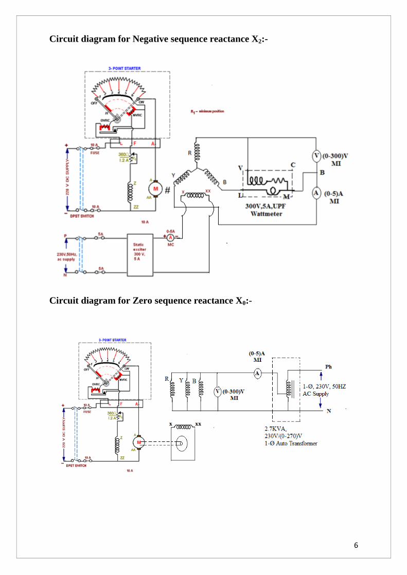
Circuit diagram for Negative sequence reactance X2:-

Circuit diagram for Zero sequence reactance X0:-

7

(ii) Short Circuit Test:-





speed.

4. Apply low voltage across the field circuit such that the rated current in the ammeter which

connect the short circuit winding of the synchronous machine.

(b) Determination of X2:-





speed.

4. Short circuit the two phases of an alternator through an ammeter and the current coil of the

wattmeter.

5. Connect the voltage coil of the wattmeter and voltmeter between the open phase and any

short circuit phase.

6. Increase the Excitation gradually in step by step such that the short circuit current should

not exceed the full load value.

(c) Determination of X0:-





speed.

4. Connect the armature winding in parallel.

5. Short circuit the field winding of an alternator.

6. Apply a low voltage of 1-Ø auto transformer and then taken the both the values of

voltmeter and ammeter of an armature winding.

8

Tabular Column:-

(a) Determination of X1 :-

(i) Open Circuit Test:-

Excitation Current If (A) Open circuit voltage (V)

(ii) Short Circuit Test:-

Excitation Current If (A) Short Circuit Current (A)

Positive sequence impedance Z1= SC

OC

I

V

Positive sequence reactance 21

211 RZX

(b) Determination of X2:-

Applied voltage (V) Short circuit current (A) Wattmeter reading (W)

Negative sequence impedance Z2=SC

OC

I

V

Power factor

SCVI

PCos

3

Negative sequence reactance SinZX 22

(c) Determination of X0:-

Short circuit voltage (V) Short circuit current (A)

Zero sequence reactance 3/0

00

I

VX

9

Precautions:-

1. Avoid the loose connections.

2. Note down the readings without parallax error.

3. Keep the field rheostat in maximum resistance position.

4. Keep the variac of the static exciter in minimum voltage output position.

Result:-

Conclusion:-

10

EXP.NO: DATE:

Circuit diagram for L-G Fault:-

11

EXP.NO: DATE:

2. FAULT ANALYSIS – I

Aim:- To find the fault currents and fault voltages when a single line to ground (L-G) fault

and line to line (L-L) faults occurred on unloaded alternator.






4 Rating 5 KVA 5 HP



7 Excitation 220V, 1A 220V, 1A



1 Ammeter

2 Voltmeter

3 Rheostat

4 Static Exciter

5 Tachometer

6 Connecting Wires

Procedure:-

(a) LG Fault:-


2. Ensure that the filed rheostat is kept in minimum resistance position and DPST switch in

off position and give the supply to DC motor and then by varying field rheostat. Let, the

motor runs at rated speed.

3. By varying the rheostat rated voltage in the voltmeter connected between the phase into be

obtained with DPST switch in open stator.

4. At this instant note down all the voltmeter and ammeter readings.

5. Now close the DPST switch under fault condition. Note down the fault currents and fault

voltages.

12

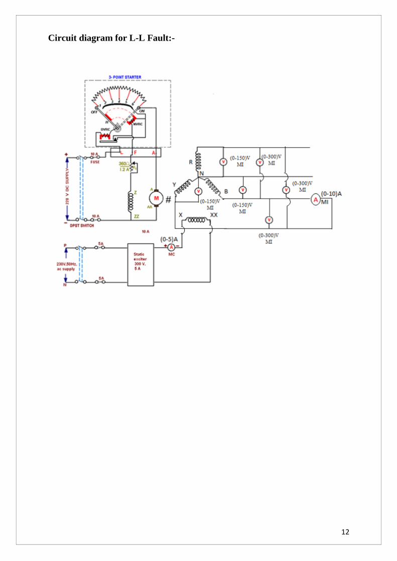
Circuit diagram for L-L Fault:-

13

(b) LL Fault:-





3. Vary the rated speed up to rated voltage in the voltmeter connected between the phasor

with DPST Switch in open position.

4. Now create a fault between the phasor Y and B, take readings of voltmeter and Ammeter.

5. Calculate Fault current using sequence impedance method.

Tabular Column:-

(a) LG Fault:-

VRN (V) VYN (V) VBN (V) IR (A) VRY (V) VYB (V) VBR (V) IF (A)

(b) LL Fault:-


Calculations:-

020 2401,1201

Ib = Ic= 0 Amp

14

(i) For LG fault

cbaa VVVV3

10

cbaa VVVV 21

3

1

cbaa VVVV 22

3

1

3

I =I=I=I a

a2a1a0

0

00

a

a

I

VZ

1

11

a

aa

I

VEZ

2

22

a

a

I

VZ

R

RNf

I

VZ

f

afault

ZZZZ

EI

3

3

021

15

(ii) For LL Fault

Ia = 0 Amp, Ib + Ic = 0

Ic = - Ib

Vb = Vc

00 aI

bba III 21

3

1

bba III 22

3

1

0fZ

1

21

aI

EZZ

21

3

ZZ

EjI fault

Precautions:-


2. Note down the readings with out parallax error.



Result:-

16

EXP.NO: DATE:

Circuit diagram for LLG Fault:-

17

EXP.NO: DATE:

3. FAULT ANALYSIS – II

Aim:- To find the fault currents and fault voltages when a double line to ground (LLG) fault

and Triple line to ground (LLLG) faults occurred on unloaded alternator.






4 Rating 3 KVA 5 HP



7 Excitation 220V 2A 220V 2A



1 Ammeter

2 Voltmeter

3 Rheostat

4 Static Exciter

5 Tachometer

6 Connecting Wires

Procedure:-

(a) LLG Fault:-





3. By varying the static exciter across the rotor of an alternator apply the rated voltage across

VRN, VYN,VBN and tabulate all readings.

4. Close the TPST switch and supply the load current and note down the readings of an

voltmeter and ammeter readings.

18

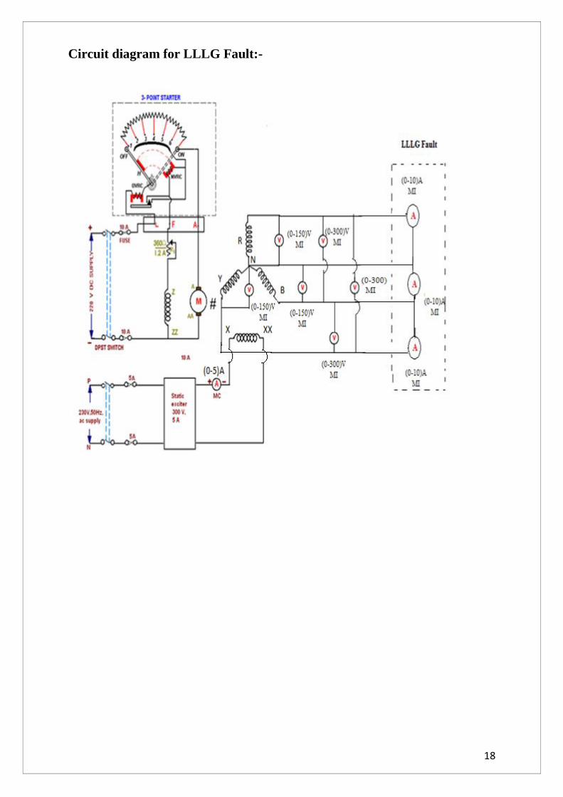
Circuit diagram for LLLG Fault:-

19

(b) LLLG Fault:-





3. Apply the rated voltage across each phase and note down the readings of an 3-Ø alternator

and tabulate them.

4. Close the TPST switch and supply the load current and note down the readings of an

voltmeter and ammeter readings.

Tabular Column:-

(a) LLG Fault:-


(b) LLLG Fault:-


20

Calculations:-

21

Precautions:-





Result:-

Conclusion:-

22

Circuit Diagram for sub transient reactance

Fig.4.1. Circuit diagram for determination of subtransient reactance of a salient pole

synchronous machine

23

EXP.NO: DATE:

4. DETERMINATION OF SUBTRANSIENT REACTANCE OF

A SALIENT POLE SYNCHRONOUS MACHINE

Aim:- To determine the subtransient direct axis reactance and quadrature axis reactance of a

salient pole synchronous machine.




2 Rated Current 8A 27.2 A


4 Rating 5 KVA 5 HP



7 Excitation 220V 2A



1 Ammeter

2 Voltmeter

3 Wattmeter

4 Auto Transformer

5 Connecting Wires

Procedure:-


2.Intially the rotor is kept in standstill, then the auto transformer is varied and a nominal

voltage is applied across the stator of the alternator. Thus the sufficient currents in the two

series connected armature windings are passed.

3.The rotor position is adjusted with hand to get maximum deflection and minimum

deflection values of armature.

4.The readings of ammeter, voltmeter and wattmeter are tabulated.

5. Calculate the Xd|| and Xq

||by using corresponding formulae’s.

24

Tabular Column:-

(i) For Maximum field current

Field

Current

IF (A)

Max.

Armature

Current Ia (A)

Excitation

voltage (v)

Power

(w)

Power

factor COSØ

Subtransient

impedance

Zq|| (Ω)

Subtransient

reactance

Xq|| (Ω)

Calculations:-

Power factor maxminIV

PCOS q

2)(1 qq CosSin

Subtransient impedance max

min| |

2)(

I

VZq

Subtransient Reactance qqq SinZX | || |

)(

(ii) For Minimum field current

Field

Current

IF (A)

Min. Armature

Current Ia (A)

Excitation

voltage (v)

Max.

Power

(w)

Power

factor COSØ

Subtransient

impedance

Zd|| (Ω)

Subtransient

reactance

Xd|| (Ω)

25

Calculations:-

Power factor minmaxIV

PCOS d

2)(1 dd CosSin

Subtransient impedance min

max| |

2)(

I

VZd

Subtransient Reactance ddd SinZX | || |

)(

Precautions:-



Result:-

Conclusion:-

26

EXP.NO: DATE:

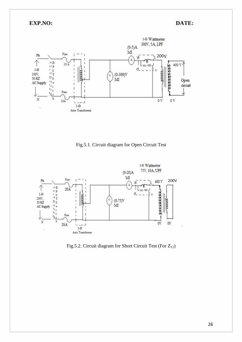
Fig.5.1. Circuit diagram for Open Circuit Test

Fig.5.2. Circuit diagram for Short Circuit Test (For Z12)

27

EXP.NO: DATE:

5. Equivalent Circuit of a 3-Ø Three Winding Transformer

Aim:- To determine the equivalent circuit parameters of a 3-Ø three winding transformer.


S.No Parameter Primary Secondary Tertiary

1 Rated Voltage 400 V 200 V 80 V

2 Rated Current 1.83A 3.6 A 9.1 A

3 Rated Power 2.2 KVA 2.2 KVA 2.2 KVA

4 Phase 3-Ø 3-Ø 3-Ø



1 Ammeter

2 Voltmeter

3 Wattmeter

4 Auto Transformer

5 3-Ø, 3 Winding

Transformer

6 Connecting Wires

Procedure:-

(i) Open circuit test:-


2. The auto transformer is kept in zero output voltage position.

3. Varying the auto transformer of variable knob and the rated voltage is applied across the

low voltage winding of 3-Ø transformer.

4.The values of no-load current, no-load voltage and input power are noted.

5.The auto transformer is brought to zero output voltage position and the DPST switch is

opened to disconnect the circuit.

28



29

(ii) Short circuit test:-


2. The auto transformer is kept in zero output voltage position.

3.Varying the auto transformer of variable knob and allow the rated currents through the HV

winding of 3-Ø transformer.

4. Note down the values of Short circuit voltage and input power.

5.The auto transformer is brought to zero output voltage position and the DPST switch is

opened to disconnect the circuit.

Tabular Column:-

(i) Open circuit test:-

No-load voltage (V) No-load current (A) Power W0 (w)

(ii) Short circuit test:-

For Z12

For Z13

For Z23

Short circuit current

ISC (A)

Short Circuit

Voltage Vsc (V)

Input Power Wsc (w)

30

Calculations:-

sc

sc

I

VZ 12 ,

sc

sc

I

VZ 13 ,

sc

sc

I

VZ 23

23131212

1ZZZZ

13122322

1ZZZZ

12132332

1ZZZZ

Precautions:-



3. Initially the auto transformer is kept in zero output voltage position.

4. Only one phase of the transformer is used to conduct the experiment.

Result:-

Conclusion:-

31

EXP.NO: DATE:

6. GAUSS-SEIDEL LOAD FLOW ANALYSIS USING MATLAB

Aim:- To solve power flow problems by the method of Gauss-Seidel using MATLAB.


S.No Apparatus Quantity

1 Personal Computer 1

2 Keyboard 1

3 Mouse 1

4 MATLAB Software 1

Procedure:-

1. Turn on your personal computer.

2. Click on the MATLAB icon of your personal computer.

3. Click the file button and select the new Blank M-file.

4. Type the program on the new M-file for corresponding bus system.

5. After completion of the program, save and run.

6. Note down the line flow and losses.

7. Close the MATLAB tool and turnoff your pc.

32

PROBLEM ON LOAD FLOW STUDIES:

For a sample power system which contains four buses, obtain the load flow analysis using

Gauss Siedal method. Treat base MVA of the system as 100MVA and the acceleration factor

as 1.6.

Bus data of the system is as follows.

Bus Number PD (MW) QD (MVAr) V∟α Remarks

1 --- --- 1.04∟0 Slack Bus

2 50 -20 --- PQ Bus

3 -100 50 --- PQ Bus

4 30 -10 --- PQ Bus

Line data of the system is as follows.

Sending end Receiving end Reactance values

in ohms

1 2 0.05+j0.15

1 3 0.10+j0.30

3 4 0.05+j0.15

2 4 0.10+j0.30

2 3 0.15+j0.45

PROGRAM ON LOAD FLOW STUDIES:

clc;

clear all;

basemva= 100;

acceleration=1.6;

accuracy=0.00001;

maxiter=50;

busdata=[1 1 1.04 0 0 0 0 0 0 0 0;

2 0 1 0 50 -20 0 0 0 0 0;

3 0 1 0 -100 50 0 0 0 0 0;

33

4 0 1 0 30 -10 0 0 0 0 0];

% IEEE BUS TEST SYSTEM

% BUS BUS VOLTAGE ANGLE ---Load--- --------Geneartor-------- static Mvar

% No Code Mag. Degree MW Mvar MW Mvar Qmin Qmax +Qc/-Ql

Busdata=[ ];

% Line code

% Bus Bus R X ½ B =1 for lines

% nl nr p.u. p.u. p.u. >1 or <1 tr.tap at bus nl

% Linedata=[ ];

linedata=[1 2 0.05 0.15 0 1;

1 3 0.1 0.3 0 1;

2 3 0.15 0.45 0 1;

2 4 0.1 0.3 0 1;

3 4 0.05 0.15 0 1];

lfybus % form the bus admittance matrix

lfgauss % Load flow solution by Gauss-seidel method

busout % Prints the power flow solution on the screen

lineflow % Computes and displays the line flow and losses

COMMANDS USED IN THE PROGRAM:

busdata matrix consists of 11 columns in which

1st column represents bus number

2nd

column represents bus code i.e., 1 for slack bus, 2 for PV bus and 3 for PQ bus

3rd

column represents voltage magnitude

4th

column represents voltage angle

5th

column represents real power demand in MW

6th

column represents reactive power demand in MVAr

7th

column represents real power generation in MW

8th

column represents reactive power generation in MVAr

9th

column represents minimum limit of reactive power in MVAr

10th

column represents maximum limit of reactive power in MVAr

34

11th

column represents reactive power injection in MVAr

linedata matrix consists of six columns in which

1st column represent sending end

2nd

column represents receiving end

3rd

column represents resistance between the sending and receiving end in ohms

4th

column represents reactance between the sending and receiving end in ohms

5th

column represents half of the susceptance in mhos

6th

column represents the line or transformer tap setting i.e., 1 for line and tap setting value

for transformer

lfybus is the command used to calculate admittance matrix

lfgauss is the command which gives power flow solution using Gauss Siedal method

busout is the command used to print the complete information about the buses

lineflow is the command used to print the line flow and line losses

Calculations:-

35

Precautions:-

1. Check and write the program with out errors.

2. Properly turn on and turn off your pc

Result:-

Conclusion:-

36

EXP.NO: DATE:

7. FAST DECOUPLED LOAD FLOW ANALYSIS USING MATLAB

Aim:- To solve power flow problems by the method of fast decoupledusing MATLAB.




2 Keyboard 1

3 Mouse 1

4 MATLAB Software 1

Procedure:-



3. Click the file button and select the new Blank M-file.

4. Type the program on the new M-file for corresponding bus system.

5. After completion of the program, save and run.

6. Note down the line flow and losses.


37

Program:-

Clear

basemva=100;

accuracy=0.001;

accel=1.8;

maxiter=100;

busdata=[1 1 1.04 0 0 0 0 0 0 0 0;

2 0 1 0 50 -20 0 0 0 0 0;

3 0 1 0 -100 50 0 0 0 0 0;

4 0 1 0 30 -10 0 0 0 0 0];

% IEEE BUS TEST SYSTEM

% BUS BUS VOLTAGE ANGLE ---Load--- --------Geneartor-------- static Mvar

% No Code Mag. Degree MW Mvar MW Mvar Qmin Qmax +Qc/-Ql

Busdata=[

];

linedata=[1 2 0.05 0.15 0 1;

1 3 0.1 0.3 0 1;

2 3 0.15 0.45 0 1;

2 4 0.1 0.3 0 1;

3 4 0.05 0.15 0 1];

% Line code

% Bus Bus R X ½ B =1 for lines

% nl nr p.u. p.u. p.u. >1 or <1 tr.tap at bus nl

Linedata=[

];

lfybus % form the bus admittance matrix

decouple % Load flow solution by fast decoupledmethod

busout % Prints the power flow solution on the screen

lineflow % Computes and displays the line flow and losses

38

Calculations:-

Precautions:-

1. Check and write the program with out errors.


Result:-

39

EXP.NO: DATE:

8. Y BUS FORMATION USING MATLAB

AIM: To obtain the Zbus matrix for the given power system using Zbus building algorithm and

to verify the same using MATLAB.

APPARATUS REQUIRED: Personal Computer with MATLAB software.

PROBLEM ON FORMATION OF Zbus:

Find the bus impedance matrix using Zbus building algorithm for the given power system

whose reactance values are as follows.


in ohms

0 1 j1.0

1 2 j0.25

0 2 j1.25

2 3 j0.05

0 3 j1.50

PROGRAM FOR FORMATION OF ZBUS USING THE GIVEN DATA:

linedata=[0 1 0 1.0;

1 2 0 0.25;

0 2 0 1.25;

2 3 0 0.05;

0 3 0 1.5];

ZBUS=zbuild(linedata)

40

OUTPUT:


zbuild is the command used to obtain the impedance matrix for the given system data using

Zbus building algorithm.

linedata matrix consists of four columns in which


2nd


3rd


4th


Result:

41

EXP.NO: DATE:

9. Y BUS FORMATION USING MATLAB

AIM: To obtain the Ybus matrix for the given power system using Direct inspection method

and to verify the same using MATLAB.

APPARATUS REQUIRED: Personal Computer with MATLAB software.

PROBLEM ON FORMATION OF Ybus:

Find the Ybus matrix for the given power system data using Direct inspection method


in ohms

1 2 j0.15

2 3 j0.10

1 3 j0.20

1 4 j0.10

4 3 j0.15

PROGRAM FOR YBUS FORMATION USING THE GIVEN DATA:

zdata=[1 2 0 0.15;

1 3 0 0.2;

1 4 0 0.1;

2 3 0 0.1;

3 4 0 0.15];

YBUS=Ybus(zdata)

42

OUTPUT:


ybus is the command used to obtain the admittance matrix for the given system data using

direct inspection method.

zdata matrix consists of four columns in which


2nd


3rd

column represents resistance between the sending and receiving end

4th

column represents reactance between the sending and receiving end

Result:

43

EXP.NO: DATE:

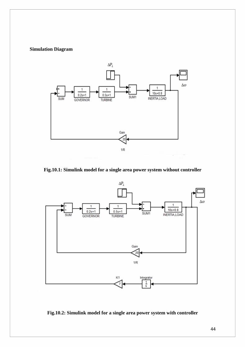
10. DEVELOP A SIMULINK MODEL FOR A SINGLE AREA LOAD

FREQUENCY CONTROL PROBLEM

Aim:- Develop a Simulink model for a single area load frequency problem and Simulate the

same by using MATLAB.




2 Keyboard 1

3 Mouse 1

4 MATLAB Software 1

Procedure:-



3. Click the Simulink button and select the new model file.

4. Connect the blocks as shown in fig 9.1 and fig 9.3.

5. After completion of the process, save and simulate.

6. Observe and draw the graph of frequency deviation step response.


44

Simulation Diagram

Fig.10.1: Simulink model for a single area power system without controller

Fig.10.2: Simulink model for a single area power system with controller

45

Model Graphs:

Fig.10.3: Frequency deviation step response without controller

Fig.10.4: Frequency deviation step response with controller

46

Precautions:-

1. Connect the blocks properly.


Result:-

Conclusion:-

47

EXP.NO: DATE:

11. NEWTON RAPHSON METHOD OF LOAD FLOW ANALYSIS USING MATLAB

AIM: To obtain load flow studies using Newton Raphson method for the given power system

data and to verify the same using MATLAB.

APPARATUS REQUIRED: Personal Computer with MATLAB Software.

PROBLEM ON LOAD FLOW STUDIES:

For a sample power system which contains four buses, obtain the load flow analysis using

Newton Raphson method. Treat base MVA of the system as 100MVA and the acceleration

factor as 1.6.

Bus data of the system is as follows.

Bus Number PG (MW) QG (MVAr) PD (MW) QD (MVAr) V∟α Remarks

1 --- --- --- --- 1.025∟0 Slack Bus

2 --- --- 400 200 1.0∟0 PQ Bus

3 300 --- --- --- 1.03∟0 PV Bus

Line data of the system is as follows.


in ohms

1 2 j0.025

1 3 j0.05

2 3 j0.025

48

PROGRAM ON LOAD FLOW STUDIES:

clc;

clear all;

busdata=[1 1 1.025 0 0 0 0 0 0 0 0;

2 0 1 0 400 200 0 0 0 0 0;

3 2 1.03 0 0 0 300 0 0 0 0];

linedata=[1 2 0 0.025 0 1;

3 2 0 0.025 0 1;

1 3 0 0.05 0 1];

basemva=100;

accel=1.6;

maxiter=50;

accuracy=0.000001;

lfybus

lfnewton

busout

lineflow


busdata matrix consists of 11 columns in which

1st column represents bus number

2nd

column represents bus code i.e., 1 for slack bus, 2 for PV bus and 3 for PQ bus

3rd

column represents voltage magnitude

4th

column represents voltage angle

5th

column represents real power demand in MW

6th

column represents reactive power demand in MVAr

7th

column represents real power generation in MW

49

8th

column represents reactive power generation in MVAr

9th

column represents minimum limit of reactive power in MVAr

10th

column represents maximum limit of reactive power in MVAr

11th

column represents reactive power injection in MVAr

linedata matrix consists of six columns in which


2nd


3rd


4th


5th

column represents half of the susceptance in mhos

6th

column represents the line or transformer tap setting i.e., 1 for line and tap setting value

for transformer

lfybus is the command used to calculate admittance matrix

lfnewton is the command which gives power flow solution using Newton Raphson method

busout is the command used to print the complete information about the buses

lineflow is the command used to print the line flow and line losses

Result:

50

EXP.NO: DATE:

12. SHORT CIRCUIT ANALYSIS FOR LINE TO GROUND FAULT AND LINE TO

LINE FAULT USING MATLAB

AIM: To obtain the short circuit analysis for line to ground fault and line to line fault in the

given power system and to verify the same using MATLAB.

APPARATUS REQUIRED: Personal Computer with MATLAB Software.

PROBLEM ON SHORT CIRCUIT ANALYSIS:

The reactance data for the power system in p.u is given in the table below on a common base

as follows.

Item Positive

sequence

reactance

Negative

sequence

reactance

Zero

sequence

reactance

G1 0.20 0.20 0.05

G2 0.10 0.10 0.25

T1 0.30 0.30 0.25

T2 0.25 0.25 0.25

L12 0.30 0.30 0.15

Obtain Positive, Negative and Zero sequence bus impedance matrices and

compute the fault current for the fault location at bus 1 in p.u for the following type of faults

a) Bolted single line to ground fault at bus 1

b) A bolted line to line fault

PROGRAM FOR SHORT CIRCUIT STUDIES:

zdata1=[0 3 0 0.2;

3 1 0 0.3;

1 2 0 0.3;

2 4 0 0.25;

4 0 0 0.1];

zdata2=zdata1;

zdata0=[0 1 0 0.25;

1 2 0 0.15;

2 0 0 0.25;

0 3 0 0.05;

0 4 0 0.25;

3 1 inf inf;

2 4 inf inf];

zbus1=zbuild(zdata1)

51

zbus0=zbuild(zdata0)

zbus2=zbus1

lgfault(zdata0,zbus0,zdata1,zbus1,zdata2,zbus2)

llfault(zdata1,zbus1,zdata2,zbus2)


zdata0, zdata1 and zdata2 represents Zero sequence, Positive sequence and Negative

sequence matrices which consists of four columns in which


2nd


3rd

column represents resistance between the sending and receiving end

4th

column represents reactance between the sending and receiving end

zbuild is the command used to obtain the impedance matrix for the given system data using

Zbus building algorithm.

lgfault is the command used to calculate the total fault current of Line to ground fault

llfault is the command used to calculate the total fault current of Line to line fault

Result:

Date post:	09-Nov-2020
Category:	Documents
Upload:	others
View:	1 times
Download:	0 times

POWER SYSTEMS & SIMULATION LABORATORYcrectirupati.com/sites/default/files/lab1/PS&S LAB IV-I.pdf5...

Documents