Power Transformer Modelling for Optimal Performance · transformer’s efficiency and voltage...

Power Transformer Modelling for Optimal

Performance School of Engineering and Information

Technology

Mohammed Alabdrbalreda Bachelor of Electrical Power Engineering

2015

I declare that the entire project is my own work or appropriately acknowledged.

Mohammed Alabdrbalreda

iii

Abstract

Power transformer efficiency is dependent on various losses. Efficiency is simply a ratio of

the power output to power input. Due to losses the efficiency of a power transformer is

always less than 100 per cent. Moreover, the transformer’s performance slightly varies

under different loads because of load-dependent losses (winding losses). The main

objective of this thesis is to find the optimum load which maximises the efficiency and

minimises the voltage regulation on a power transformer operated at its rated voltage.

The complete equivalent circuit of a power transformer is developed with various losses

taken into account such as winding losses, leakage fluxes, core losses, and magnetisation

currents. The model parameters are found by carrying out laboratory measurements.

Once the complete equivalent circuit is developed, it is used to calculate the efficiency

and the voltage regulation under different loading cases. A simulated model on ICAP is

also used to validate the experimental results. A sensitivity analysis is also conducted in

this project to see the effect of variations in the parameters on the transformer’s

performance.

Finally, the design parameters of a power transformer that can be optimized to reduce

losses are considered in this project. The design parameters are related to the electrical

parameters of the transformer by mathematical models. The effect of those design

parameters on the transformer’s performance is supported by some papers related to

design optimisation. This involves the evolution of power transformers design throughout

history and the research being carried out for loss reduction. Other factors such as cost

and operation environment are not taken into account in this project as it is only focused

on efficiency optimization.

iv

The key findings of this project can be summarized as follows; the resistive load has the

poorest voltage regulation. The capacitive load has the lowest voltage regulation and it is

always negative. The transformer’s maximum efficiency is observed at 60 per cent of the

rated load. This is proved by laboratory based experiments and ICAPS simulations. The

key design parameters that can be optimized to improve the efficiency are the core

lamination thickness, material electrical resistivity, and maximum flux density.

v

Acknowledgment

I would like to take the chance in this acknowledgment to thank my project supervisor Dr.

Sujeewa Hettiwatte for the academic guidance and motivation he has been supporting to

me during this project as well as previous units. Dr. Sujeewa has a very good insight at

power transformers. Therefore, he has been supporting me with his insightful comments

and recommendations. I completed this project under Dr. Sujeewa’s supervision and has

become, therefore a possible graduate engineer. It is really an honour having Dr. Sujeewa

as my supervisor since I built my electrical engineering knowledge with his support.

I would like to also thank the academic staff in the School of Engineering and IT at

Murdoch University including Dr. Gregory Crebbin, Dr. Gareth Lee, Dr. Martina Calais, Dr.

Trevor Pryor and Prof. Graeme Cole.

I am also grateful to my sponsor, the Saudi Arabian Cultural Mission, for the funding

supplied for the whole degree including this project.

I am thankful to Mr Alnasser Majed, who helped me throughout my studies and also

proofread this report.

Finally, I am greatly thankful to my family including my parents, my older brothers and

my wife for their encouragement to complete my degree and their financial support.

vi

Table of Contents

Abstract ...................................................................................................................... iii

Acknowledgment ......................................................................................................... v

List of Figures ............................................................................................................ viii

List of Tables ............................................................................................................... ix

Acronyms ........................................................................... Error! Bookmark not defined.

1.0 Introduction ........................................................................................................... 1

1.1 Project Objectives .......................................................................................................... 2

1.2 Scope of Work ................................................................................................................ 2

1.3 Literature Review ........................................................................................................... 3

1.4 Determination of Transformer Parameters ..................................................................... 8

1.4.1 Open-Circuit Test ............................................................................................................... 9

1.4.2 Short-Circuit Test ............................................................................................................. 11

1.5 Voltage Regulation ....................................................................................................... 13

2.0 System Model ....................................................................................................... 15

3.0 Experimental Measurements ................................................................................ 16

3.1 Open-Circuit Test.......................................................................................................... 16

3.2 Short-Circuit Test .......................................................................................................... 20

3.3 Voltage Regulation and Efficiency ................................................................................. 24

3.4 Winding Resistance Segregations .................................................................................. 29

3.4.1 Determination of Winding Resistance by Energizing the Transformer ........................... 30

3.4.2 Measuring the Windings Resistance Using DMM ........................................................... 34

4.0 Simulations ........................................................................................................... 36

vii

4.1 No-Load Voltage ........................................................................................................... 36

4.2 Voltage Regulation and Efficiency Simulations .............................................................. 37

5.0 Maximum Efficiency Criterion ............................................................................... 41

6.0 Sensitivity Analysis ............................................................................................... 44

6.1 Electrical Parameters .................................................................................................... 44

6.1.1 Core-loss Resistance (𝑹𝒄) ................................................................................................ 44

6.1.2 Magnetizing Reactance (𝑿𝑴) ......................................................................................... 47

6.1.3 Equivalent Winding Resistance (𝑹𝒆𝒒) ............................................................................ 48

6.1.4 Equivalent Leakage Reactance (𝑿𝒆𝒒) ............................................................................. 51

6.2 Physical Design Parameters .......................................................................................... 51

6.2.1 Core losses ....................................................................................................................... 52

6.2.2 Winding Losses ................................................................................................................ 62

7.0 Conclusions and Future Work ................................................................................ 72

8.0 Annotated Bibliography ........................................................................................ 74

9.0 References ............................................................................................................ 76

10.0 Appendix ............................................................................................................ 79

viii

List of Figures

Figure 1 Shell-Type Core..................................................................................................................... 4

Figure 2 Core Type ............................................................................................................................. 4

Figure 3 Transformer Power Flow [3] ................................................................................................ 8

Figure 4 Transformer Equivalent Circuit Under Open-circuit Conditions ........................................ 10

Figure 5 Current Phasor Diagram ..................................................................................................... 11

Figure 6 Transformer Equivalent Circuit Under Short-circuit Conditions ........................................ 12

Figure 7 Voltage Phasor Diagram ..................................................................................................... 13

Figure 8 Open Circuit Test Experiment [7] ....................................................................................... 16

Figure 9 Transformer Exact Equivalent Circuit Open-circuited ........................................................ 18

Figure 10 Short-Circuit Test Experiment [7] ..................................................................................... 20

Figure 11 Transformer Exact Equivalent Circuit Short-Circuited ..................................................... 22

Figure 12 Transformer Model .......................................................................................................... 24

Figure 13 Voltage Regulation and Efficiency Experiment [7] ........................................................... 24

Figure 14 Regulation Curves............................................................................................................. 29

Figure 15 Primary Winding Resistance Measurement Under Open-circuit Conditions [7] ............. 31

Figure 16 Primary Winding Resistance Measurement Under Short-circuit Conditions [7] ............. 32

Figure 17 Secondary Winding Resistance Measurement Under Open-circuit Conditions [7] ......... 33

Figure 18 Secondary Winding Resistance Measurement Under Short-circuit Conditions [7] ......... 33

Figure 19 Regulation Curves (based on simulation results) ............................................................. 40

Figure 20 Efficiency vs Load Current ................................................................................................ 42

Figure 21 Load Current at Maximum Efficiency ............................................................................... 43

Figure 22 Efficiency against PF ......................................................................................................... 43

Figure 23 Efficiency Improvement due to Increased Core-loss Resistance ..................................... 46

Figure 24 Increased Voltage Regulation due to Variations in the Equivalent Winding Resistance . 50

ix

Figure 25 Eddy Current Loss vs Lamination Thickness ..................................................................... 57

Figure 26 Eddy Current loss Against Electrical Resistivity ................................................................ 58

Figure 27 “Magnetization curves of 9 ferromagnetic materials, showing saturation. 1.Sheet steel,

2.Silicon steel, 3.Cast steel, 4.Tungsten steel, 5.Magnet steel, 6.Cast iron, 7.Nickel, 8.Cobalt,

9.Magnetite” [17] ............................................................................................................................. 59

Figure 28 Eddy Current Loss vs. 𝐁𝐦𝐚𝐱 ............................................................................................ 60

Figure 29 Hysteresis Loss vs. 𝐁𝐦𝐚𝐱 ................................................................................................. 60

Figure 30 Core Losses vs 𝐁𝐦𝐚𝐱 ....................................................................................................... 61

Figure 31 Windings arrangment of single-phase transformer [3] ................................................... 70

List of Tables

Table 1 LabVolt Series (8341-0A) Transformer’s Specifications ...................................................... 15

Table 2 Open-Circuit & Short-Circuit Tests Summary ...................................................................... 23

Table 3 Resistive Load ...................................................................................................................... 26

Table 4 Inductive Load ..................................................................................................................... 26

Table 5 Capacitive Load .................................................................................................................... 27

Table 6 Voltage Regulation .............................................................................................................. 28

Table 7 Efficiency for Each Load Type at Variable Impedance ......................................................... 28

Table 8 Winding Resistance Segregation ......................................................................................... 34

Table 9 No-Load Simulation Input Data ........................................................................................... 36

Table 10 No-Load Voltage Simulation Results ................................................................................. 37

Table 11 Resistive Load Simulation Results ..................................................................................... 37

Table 12 Inductive Load Simulation Results ..................................................................................... 38

Table 13 Capacitive Load Simulation Results ................................................................................... 38

Table 14 Simulation results after modelling an inductive load using an ideal inductor in series with

a resistor ........................................................................................................................................... 39

x

Table 15 Core-Loss Resistance 10% Increase ................................................................................... 45

Table 16 Core-Loss Resistance 10% Increase ................................................................................... 45

Table 17 Efficiency Improvement due to Core-loss Resistance Reduction ...................................... 47

Table 18 Magnetizing Reactance 10% Increase ............................................................................... 48

Table 19 Winding Resistance 10% Increase ..................................................................................... 48

Table 20 Winding Resistance 10% Decrease .................................................................................... 49

Table 21 Increased Voltage Regulation due to Increase in the Equivalent Winding Resistance ..... 50

Table 22 Leakage Reactance 10% Increase ...................................................................................... 51

Table 23 AK Non-oriented Electrical Steel M27 ............................................................................... 57

Table 24 Design Parameters of Transformer Used for Winding Type Analysis ............................... 66

Table 25 Winding Type Analysis Results .......................................................................................... 69

Table 26 Core Losses for Different Materials ................................................................................... 79

Table 27 AK Non-oriented Electrical Steel Resistivity ...................................................................... 79

Table 28 Eddy Current Loss vs Lamination Thickness ...................................................................... 80

Table 29 Eddy Current Loss vs Electrical Resistivity ......................................................................... 80

Table 30 Core Losses vs Flux Density ............................................................................................... 81

xi

Symbols

𝐵𝑚𝑎𝑥=Maximum flux density

𝐼𝐶= Current loss due to core resistance

𝐼𝐿= Load current

𝐼𝐿𝜂=Load current at maximum efficiency

𝐼𝑀=Magnetisation current

𝐼𝑆𝐶=Short-circuit current across the secondary terminal

𝐼𝑖𝑛= The input current from power supply

𝑁𝑃=Number of primary winding turns

𝑁𝑆=Number of secondary winding turns

𝑃ℎ=Hysteresis loss

𝑃𝐶=Copper loss

𝑃𝑂=Output power delivered to load

𝑃𝑒=Eddy current loss

𝑃𝑖𝑛=Input power from power supply

𝑃𝑚=Core power loss

𝑅𝐿=Load Resistance

𝑅𝑃=Primary winding resistance

xii

𝑅𝑆=Secondary winding resistance

𝑅𝑐=Core-loss resistance

𝑅𝑒𝑞=Equivalent winding resistance referred to primary side

𝑉𝐹𝐿=Load voltage at full-load conditions

𝑉𝑁𝐿=Voltage across secondary terminals with no load attached

𝑉𝑃= Primary terminal voltage

𝑉𝑆=Secondary terminal voltage

𝑉𝑋𝑒𝑞=Voltage across 𝑋𝑒𝑞

𝑉𝑖𝑛=Input voltage

𝑋𝑀=Magnetization reactance

𝑋𝑃=Primary winding reactance

𝑋𝑆=Secondary winding reactance

𝑋𝑒𝑞=Equivalent winding reactance referred to primary side

𝑍𝐿=Load impedance

Ω=Ohm

𝑎=Transformer turns ratio

𝑡=Lamination thickness

𝜂=Transformer Efficiency

xiii

𝛷𝑀=Maximum flux

𝜌=Electrical resistivity

Acronyms

HV=High voltage

LV=Low voltage

𝑃𝐹=Power factor

𝑉𝑅=Voltage regulation

1

1.0 Introduction

In this project, the equivalent model of a single-phase power transformer is developed to

analyse its performance under various loads using the electrical circuits simulator Spice

ICAPS as well as carrying out laboratory based experiments. In particular, the

performance variation of interest in this project is that of the load voltage due to load-

dependent losses as well as the efficiency. High load-dependent losses can lead to

undesirable wide variations in the load voltage in weakly designed power transformers or

by exceeding the load limitations of the transformer. The measure of such variations is

called voltage regulation which is minimized in an efficient transformer. Therefore, the

methods of controlling such losses will be discussed in this project.

The model parameters of the equivalent circuit are first determined by carrying out two

simple procedures in the laboratory called the open-circuit test and the short-circuit test.

After developing the complete equivalent circuit, a simulated model is built which will be

also used to analyse the transformers performance.

This section covers the literature review associated with voltage regulation and its related

losses. The literature describes the methodologies used to control voltage regulation and

optimize the transformer’s efficiency. The literature associated with the design aspects of

a power transformer is also covered.

The second part of this project covers the design parameters that can be optimized in

order to reduce all kinds of losses in the transformer, and thereby maximise the

efficiency.

2

1.1 Project Objectives

The objective of this project is to investigate on the effect of load variation on the

performance of a single-phase transformer using both laboratory experiments and a

computer based simulator Spice ICAPS. The main points of interest are to test the

transformer’s efficiency and voltage regulation while varying the load at the rated

voltage. The first aim of the project is to find the optimum load which maximises the

efficiency and minimises the voltage regulation. It identifies the maximum efficiency

criterion of a power transformer and the load current at these conditions. The

transformer is operated under rated input conditions with secondary terminals open-

circuited in order to find the fixed losses (core losses) and their related impedances. It will

also be operated at the rated output with the secondary terminal short-circuited in order

to find the windings resistance and leakage reactance.

The second part of the project aims to optimise the key design parameters of a

transformer operating under rated conditions to improve its efficiency. This includes the

design parameters associated with both the core losses (no-load losses) and variable

losses. The core losses considered in this project are the hysteresis loss and eddy currents

loss. Different types of windings will be considered in order to minimise the copper loss

(variable loss).

1.2 Scope of Work

The steps undertaken in this project are summarised as follows:

-selection of a LabVolt single-phase transformer available in the laboratory

-Experimental measurements (open-circuit and short-circuit tests)

3

-Developing the complete equivalent circuit

-Experimentally varying the load at the rated voltage to test the efficiency and voltage

regulation

-Building a simulated model using the model parameters from experimental

measurements on ICAPS

-Utilizing ICAPS to verify the experimental results

-Detailed research on the design parameters and relating them to electrical parameters

by mathematical models.

1.3 Literature Review

This section covers the literature reviewed for the purpose of this project. The major

losses of a power transformer are discussed. Moreover, a maximum efficiency criterion is

considered since efficiency optimization is one of the project aims.

Core losses:

The core loss is dependent on the laminations it is made of. Thinner laminations make the

core more flux-permeable between the primary and secondary windings. A transformer is

said to be efficient if most of the flux is transferred between the winding. The core

lamination material properties determine the core permeability. Silicon, for example, has

a property of low magnetic losses which in turn optimizes the transformer’s efficiency.

The common laminations thickness ranges from 0.35 to 0.61 mm [1].

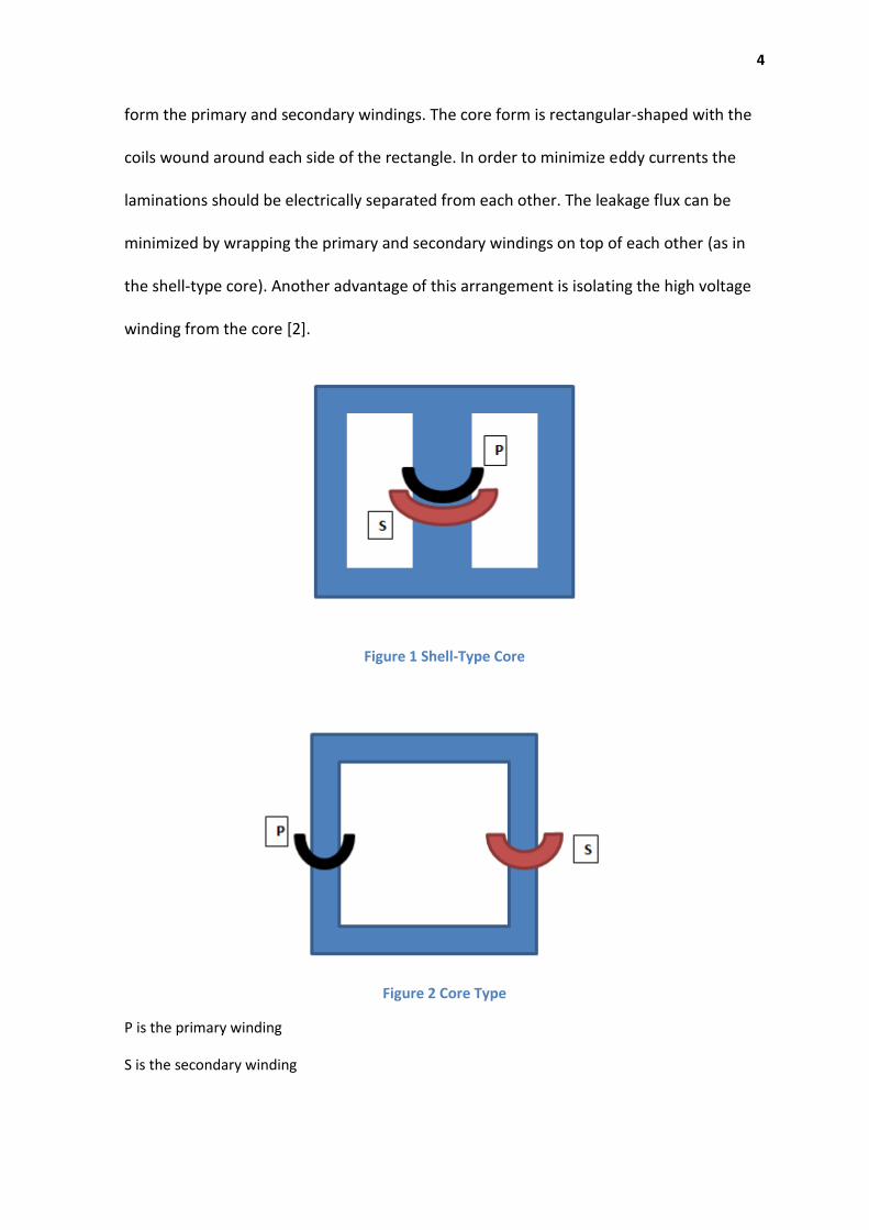
There are two types of core construction called shell form and core form. The shell form

is composed of three laminated limbs (or more). Two coils wound around the centre limb

4

form the primary and secondary windings. The core form is rectangular-shaped with the

coils wound around each side of the rectangle. In order to minimize eddy currents the

laminations should be electrically separated from each other. The leakage flux can be

minimized by wrapping the primary and secondary windings on top of each other (as in

the shell-type core). Another advantage of this arrangement is isolating the high voltage

winding from the core [2].

Figure 1 Shell-Type Core

Figure 2 Core Type

P is the primary winding

S is the secondary winding

5

Winding Losses:

The flow of the load current through the winding causes some resistive loss. This type of

loss varies with the square of the load current. There is also load-dependent eddy current

loss due to the leakage flux cutting the winding. The resistive loss cannot be totally

eliminated, but it can be minimized by transformer designers. Using a high-conductivity

copper for the winding is important to minimize the resistive loss. Lower number of

winding turns and bigger cross-sectional area of the turn conductor also reduce the

resistive losses. However, reducing the number of turns implies that 𝛷𝑀 has to be

increased which in turn requires a bigger core cross-section. Increasing the core core-

section has to be traded against the resulting iron loss. Therefore, the optimum design of

the frame (core cross-section) has to satisfy all factors [3].

The eddy current loss in the winding flows in complex paths. The leakage flux cutting

through the winding causes axial and radial flux variations at a point in space at any time.

Consequently, there are voltages induced that result in currents flowing at right angles to

the varying flux. The path resistance of these currents is inversely proportional to their

magnitude. This resistance can be minimized by using a winding conductor with smaller

cross-section. Alternatively, the winding conductor can be subdivided into several

insulated strands [3]. The resulting cost increase is not considered in this project as it is

mainly concerned with efficiency optimization.

There is another kind of load-dependent eddy currents lost in the tanks and structural

steelwork (core). However, these currents are relatively small compared to the total load

losses. These currents can be minimized by controlling the leakage flux again [3].

6

Magnetization current:

The current flowing through the primary side of a transformer with its secondary terminal

open-circuited is the current required to produce flux in a ferromagnetic core. This

current comprises the magnetization current and the core-loss currents. The

magnetization current, 𝐼𝑀, is the current required to produce the total flux on the

primary side. The core-loss current, 𝐼𝐶, is composed of hysteresis and eddy current losses

(see Figure 4) [2]. For an efficient transformer, the core-loss current should be minimized

by designers. The magnetization current is not sinusoidal and has higher harmonics due

to the magnetic saturation in the core. Once the core is saturated, a further small

increase in the peak flux would require a large increase in the magnetization current. The

magnetization current lags the voltage applied across the primary terminal of the

transformer and the current through the core loss resistance 𝑅𝑐 by 90° (see Figure 5) [4].

The core-loss current makes up the hysteresis and eddy current losses in the core. The

peak eddy current in the core is reached when the flux passing through it is zero.

Therefore, the total core-loss current is greatest when the flux passing through the core is

zero [2].

Inrush current

The inrush current is the maximum, instantaneous input current drawn by an electrical

device when turned on [5]. When a power transformer is energized, a transient current

significantly higher than the rated load current can flow through the transformer’s

terminals for several cycles. Inrush current controllers can be designed by predicting the

residual flux that remains in the transformer’s core at all times. However, the real

7

challenge is to determine the transient magnetic flux in the transformer’s core. The

inrush current can affect the magnetic property of the core permanently. Consequently,

the core becomes less flux-permeable which in turn affects the transformer’s efficiency

[5].

Maximum Efficiency Criterion:

The efficiency of a power transformer is the ratio of its output power to its input power.

In practice, the efficiency is always less than 100 per cent due to fixed and variable losses.

The core loss consists of eddy current and hysteresis losses. In order to minimize the eddy

current loss, thinner core laminations are used. The hysteresis loss depends on the core

material’s magnetic properties. The core loss is fixed since the flux in the core is constant

[1].

On the other hand, the copper loss is dependent on the load current flowing through the

transformer’s windings. This loss is given by equation 1 below.

𝑃𝑐 = 𝐼𝑖𝑛2 𝑅𝑒𝑞 (1)

Where,

𝐼𝑖𝑛 is the input current flowing the primary winding

𝑅𝑒𝑞 is the equivalent winding resistance referred to the primary side (see Figure 12)

It can be seen from the equation above that the copper loss varies as the square of the

current in each winding. Therefore, the copper loss is proportional to the load current.

8

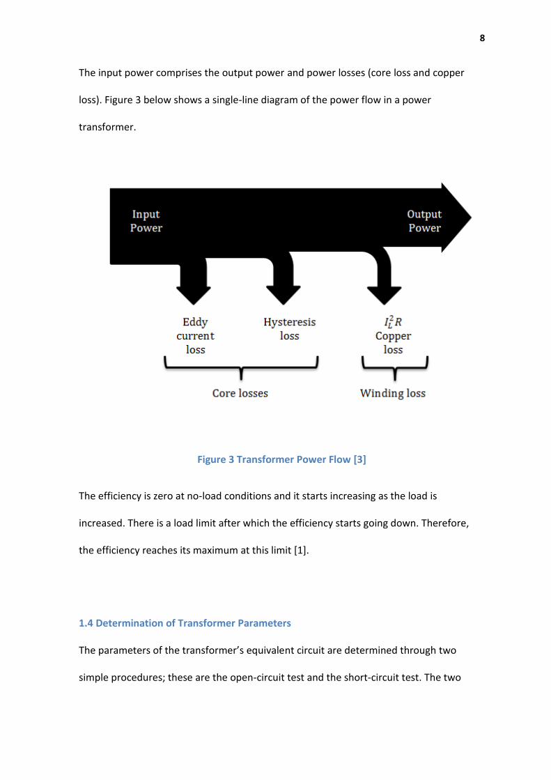
The input power comprises the output power and power losses (core loss and copper

loss). Figure 3 below shows a single-line diagram of the power flow in a power

transformer.

Figure 3 Transformer Power Flow [3]

The efficiency is zero at no-load conditions and it starts increasing as the load is

increased. There is a load limit after which the efficiency starts going down. Therefore,

the efficiency reaches its maximum at this limit [1].

1.4 Determination of Transformer Parameters

The parameters of the transformer’s equivalent circuit are determined through two

simple procedures; these are the open-circuit test and the short-circuit test. The two

9

tests are carried out in the laboratory to take the measurements needed to calculate the

model parameters.

1.4.1 Open-Circuit Test

This test is carried out to determine magnetizing reactance, core-loss resistance and the

fixed power loss of the transformer (core-loss). The power supply must be operated at

the rated frequency of the transformer. In this test, one terminal is open-circuited while

the other is connected to the power supply. It is safer to excite the low-voltage side of

the transformer even though either side can be excited [1]. However, low-voltage power

supply is always available in laboratories while high-voltage supply might not be so. In

this project, the transformer model was initially (240/240V), but the maximum measured

input voltage was significantly below 240. Therefore, a decision was made to change the

transformer model to (208/240V). Since the secondary terminal is open-circuited, there is

no current flowing through it. Ideally, there is no current flowing through the primary

terminal under open-circuit conditions. The primary winding impedance is much smaller

than the equivalent impedance of the excitation branch. Therefore, it is neglected as

equation 2 shows in section 3.1. The resulting equivalent circuit of the transformer is

shown in Figure 4

10

Figure 4 Transformer Equivalent Circuit Under Open-circuit Conditions

It can be seen from Figure 4 above that the input current is only supplying the excitation

current in this case. The excitation current is composed of the magnetizing current 𝐼𝑀 ,

which is responsible for establishing the magnetic flux in the core, and the core-loss

current 𝐼𝐶 . The only power loss in this case is the core-loss which can be measured by a

wattmeter across the primary terminal. This kind of power loss is fixed regardless of

variations in the load [1].

Since the core-loss is modelled by the resistance, 𝑅𝐶, the core-loss current is in phase

with the supply voltage. The magnetizing current, on the other hand, lags the supply

voltage by 90°, since the magnetizing component is modelled by an inductive reactance

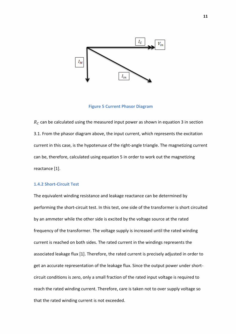
𝑋𝑀. Figure 5 below shows the phaser diagram of these vectors.

11

Figure 5 Current Phasor Diagram

𝑅𝐶 can be calculated using the measured input power as shown in equation 3 in section

3.1. From the phasor diagram above, the input current, which represents the excitation

current in this case, is the hypotenuse of the right-angle triangle. The magnetizing current

can be, therefore, calculated using equation 5 in order to work out the magnetizing

reactance [1].

1.4.2 Short-Circuit Test

The equivalent winding resistance and leakage reactance can be determined by

performing the short-circuit test. In this test, one side of the transformer is short circuited

by an ammeter while the other side is excited by the voltage source at the rated

frequency of the transformer. The voltage supply is increased until the rated winding

current is reached on both sides. The rated current in the windings represents the

associated leakage flux [1]. Therefore, the rated current is precisely adjusted in order to

get an accurate representation of the leakage flux. Since the output power under short-

circuit conditions is zero, only a small fraction of the rated input voltage is required to

reach the rated winding current. Therefore, care is taken not to over supply voltage so

that the rated winding current is not exceeded.

12

The measurements can be taken on either side again, but it is safer to perform it on the

high-voltage side. 𝑉𝑆 is zero in this case since the secondary terminal is short-circuited.

Consequently, 𝑉𝑃 is also zero under short-circuit conditions [5].

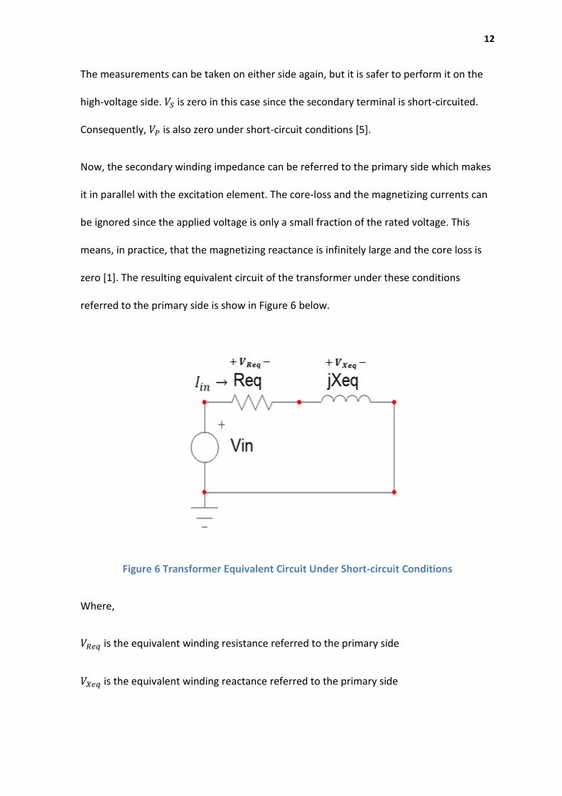
Now, the secondary winding impedance can be referred to the primary side which makes

it in parallel with the excitation element. The core-loss and the magnetizing currents can

be ignored since the applied voltage is only a small fraction of the rated voltage. This

means, in practice, that the magnetizing reactance is infinitely large and the core loss is

zero [1]. The resulting equivalent circuit of the transformer under these conditions

referred to the primary side is show in Figure 6 below.

Figure 6 Transformer Equivalent Circuit Under Short-circuit Conditions

Where,

𝑉𝑅𝑒𝑞 is the equivalent winding resistance referred to the primary side

𝑉𝑋𝑒𝑞 is the equivalent winding reactance referred to the primary side

13

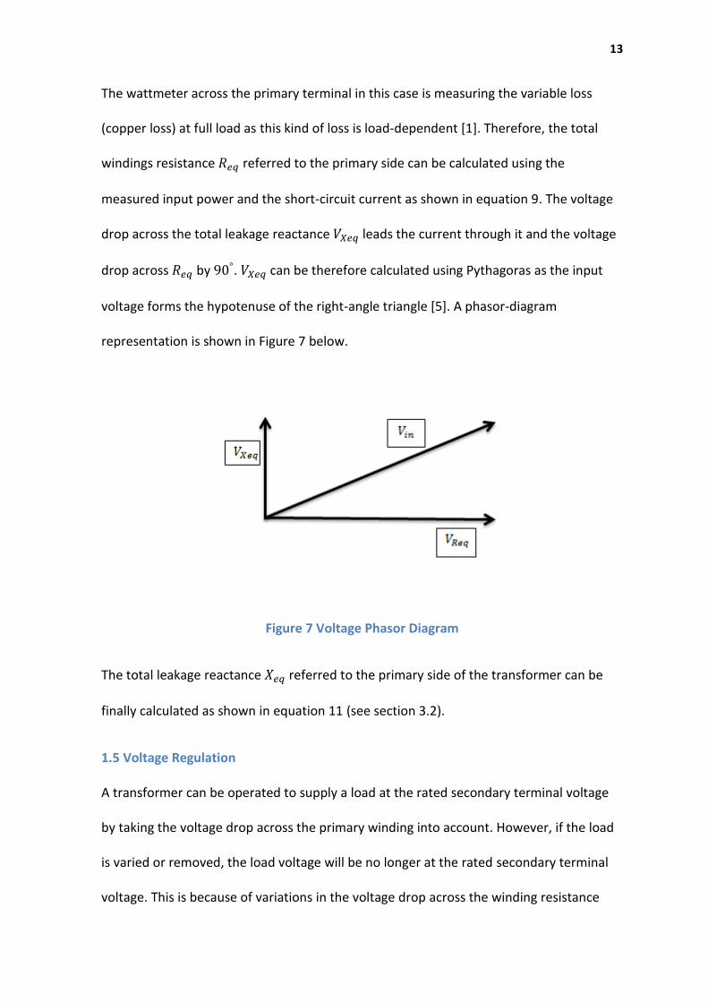
The wattmeter across the primary terminal in this case is measuring the variable loss

(copper loss) at full load as this kind of loss is load-dependent [1]. Therefore, the total

windings resistance 𝑅𝑒𝑞 referred to the primary side can be calculated using the

measured input power and the short-circuit current as shown in equation 9. The voltage

drop across the total leakage reactance 𝑉𝑋𝑒𝑞 leads the current through it and the voltage

drop across 𝑅𝑒𝑞 by 90°. 𝑉𝑋𝑒𝑞 can be therefore calculated using Pythagoras as the input

voltage forms the hypotenuse of the right-angle triangle [5]. A phasor-diagram

representation is shown in Figure 7 below.

Figure 7 Voltage Phasor Diagram

The total leakage reactance 𝑋𝑒𝑞 referred to the primary side of the transformer can be

finally calculated as shown in equation 11 (see section 3.2).

1.5 Voltage Regulation

A transformer can be operated to supply a load at the rated secondary terminal voltage

by taking the voltage drop across the primary winding into account. However, if the load

is varied or removed, the load voltage will be no longer at the rated secondary terminal

voltage. This is because of variations in the voltage drop across the winding resistance

14

and leakage reactance which is load-dependent. Therefore, the voltage regulation is a

measure of the net change in the secondary winding voltage from no load to full load for

the same primary winding voltage expressed as a percentage of the rated voltage [1]. The

lower the voltage regulation, the more efficient the transformer is.

15

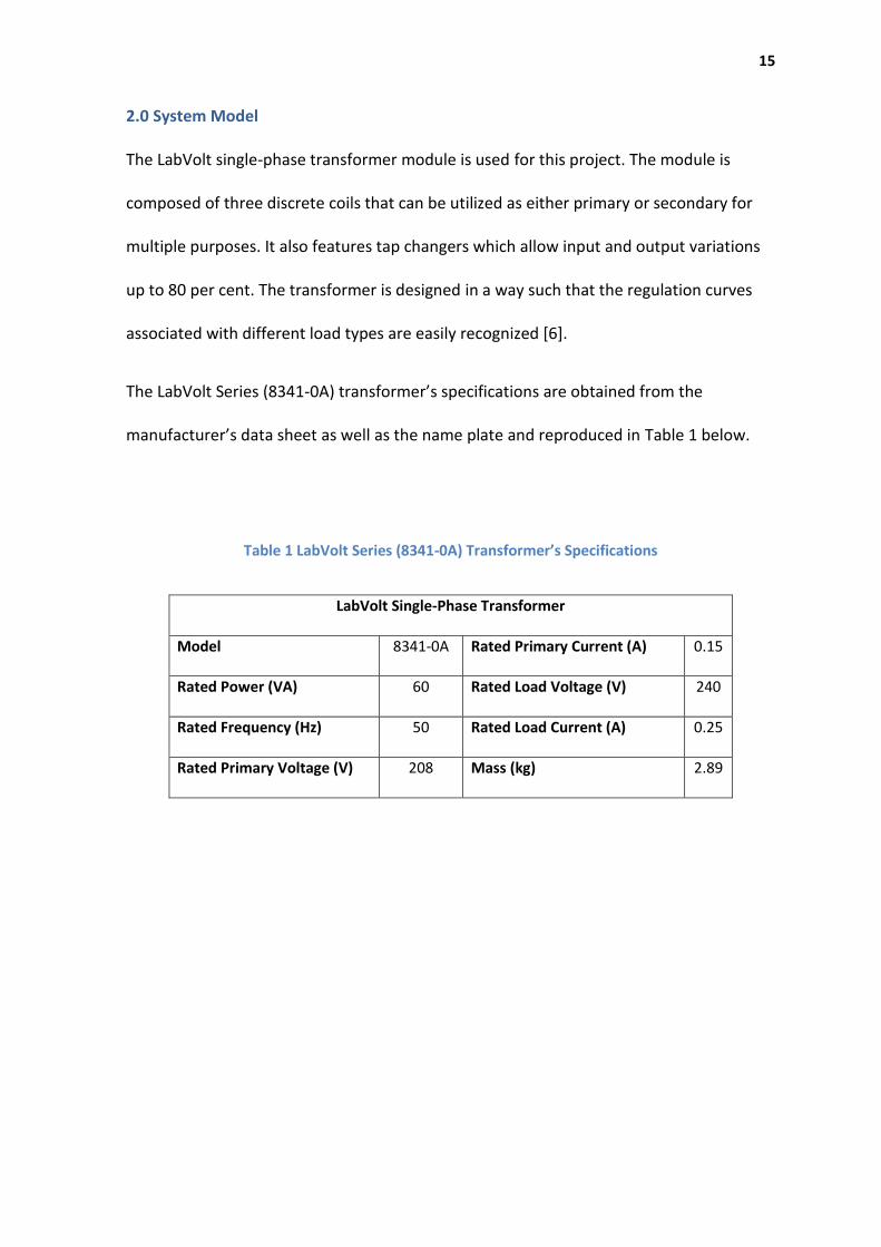
2.0 System Model

The LabVolt single-phase transformer module is used for this project. The module is

composed of three discrete coils that can be utilized as either primary or secondary for

multiple purposes. It also features tap changers which allow input and output variations

up to 80 per cent. The transformer is designed in a way such that the regulation curves

associated with different load types are easily recognized [6].

The LabVolt Series (8341-0A) transformer’s specifications are obtained from the

manufacturer’s data sheet as well as the name plate and reproduced in Table 1 below.

Table 1 LabVolt Series (8341-0A) Transformer’s Specifications

LabVolt Single-Phase Transformer

Model 8341-0A Rated Primary Current (A) 0.15

Rated Power (VA) 60 Rated Load Voltage (V) 240

Rated Frequency (Hz) 50 Rated Load Current (A) 0.25

Rated Primary Voltage (V) 208 Mass (kg) 2.89

16

3.0 Experimental Measurements

A set of laboratory experiments is carried out in order to find the model parameters and

test the transformer’s performance under various loads. The aim of each experiment,

procedure and results are discussed in sections (3.1-3.4).

3.1 Open-Circuit Test

The aim of this experiment is to find the core resistance and the magnetizing reactance.

The rated voltage is applied to the primary side of the transformer, while keeping the

secondary open. The input voltage, current and power was measured.

Equipment List

1 x LabVolt Power Supply; 1 x Single Phase Transformer unit; 1 x Voltech PM-300 Power

Analyser

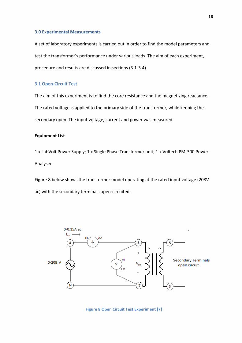
Figure 8 below shows the transformer model operating at the rated input voltage (208V

ac) with the secondary terminals open-circuited.

Figure 8 Open Circuit Test Experiment [7]

17

Where, 4-N is the AC power supply terminals; 𝐼𝑖𝑛 is the input current (on the primary

side); 𝑉𝑖𝑛 is the voltage applied to the primary side; 3-7 is the low-voltage terminals of the

single phase transformer unit; 5-6 is the high-voltage terminals with a rated voltage of

240V AC.

Procedure

1. The circuit shown in Figure 8 is connected.

2. The power supply is switched on and adjusted to 208V ac as indicated by the power

analyser (PM-300).

3. The input voltage, input current and input power are measured and recorded in Table

2.

4. The power supply is returned to zero and switched off.

Under these operation conditions, all the input current flows through the excitation

branch. Therefore, all the power loss is caused by the core [1]. Using the measurements

in Table 2 the core-loss resistance, 𝑅𝑐, and the magnetization reactance, 𝑋𝑀, can be

determined.

The equivalent circuit was used to calculate 𝑅𝑐 and 𝑋𝑀 as shown in Figure 9 below.

18

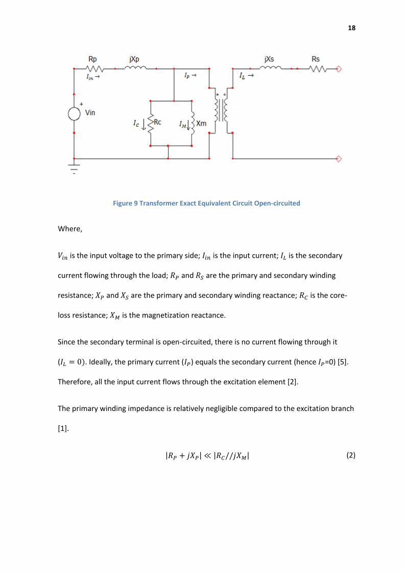
Figure 9 Transformer Exact Equivalent Circuit Open-circuited

Where,

𝑉𝑖𝑛 is the input voltage to the primary side; 𝐼𝑖𝑛 is the input current; 𝐼𝐿 is the secondary

current flowing through the load; 𝑅𝑃 and 𝑅𝑆 are the primary and secondary winding

resistance; 𝑋𝑃 and 𝑋𝑆 are the primary and secondary winding reactance; 𝑅𝐶 is the core-

loss resistance; 𝑋𝑀 is the magnetization reactance.

Since the secondary terminal is open-circuited, there is no current flowing through it

(𝐼𝐿 = 0). Ideally, the primary current (𝐼𝑃) equals the secondary current (hence 𝐼𝑃=0) [5].

Therefore, all the input current flows through the excitation element [2].

The primary winding impedance is relatively negligible compared to the excitation branch

[1].

|𝑅𝑃 + 𝑗𝑋𝑃| ≪ |𝑅𝐶//𝑗𝑋𝑀| (2)

19

The approximation made in equation 2 implies that 𝑅𝐶 is the only resistance dissipating

power in this case [1]. The input voltage and the input power can be used to calculate 𝑅𝐶

as equation 3 shows below.

𝑅𝐶 =

𝑉𝑖𝑛2

𝑃𝑖𝑛 (3)

The current flowing through this resistor can be calculated as shown in equation 4 below.

𝐼𝐶 =

𝑉𝑖𝑛

𝑅𝐶 (4)

𝐼𝑖𝑛 is the phasor sum of 𝐼𝐶 and the current through the magnetization reactance, 𝐼𝑀.

Since 𝑋𝑀 is an inductive reactance, the current through it lags the input voltage (and 𝐼𝐶)

by 90° [1]. 𝐼𝑀 can be calculated using equation 5 below.

𝐼𝑀 = √𝐼𝑖𝑛

2 − 𝐼𝐶2 (5)

Finally, 𝑋𝑀 can be calculated using Ohm’s law as equation 6 shows.

𝑋𝑀 =

𝑉𝑖𝑛

𝐼𝑀

(6)

20

3.2 Short-Circuit Test

This experiment was carried out to determine the equivalent winding resistance and

reactance. The secondary terminal was short circuited by an ammeter while taking

measurements of the input current, voltage and power.

Equipment List


Analyser; 1 x Digital Multi Meter (DMM) UNI-T UT803

Figure 10 below shows the circuit configuration of this experiment. The transformer

secondary short-circuit current is set at full-load conditions (𝐼𝐿 = 0.25 𝐴).

Figure 10 Short-Circuit Test Experiment [7]

Where,

4-N is the power supply terminals; 𝐼𝑖𝑛 is the input current (on the primary side); 𝑉𝑖𝑛 is the

voltage applied to the primary side; 3-7 are the low-voltage terminals of the single phase

21

transformer unit; 5-6 are the high-voltage terminals; 𝐼𝑆𝐶 is the short-circuit current

flowing through the secondary terminals.

Procedure


2. The power supply is switched on and the input voltage is increased until the short-

circuit current reaches the full load current (0.25A) as indicated by the ammeter 𝐼𝑆𝐶.

3. The input voltage, input current and input power are measured and recorded in

Table 2.


Since the secondary terminal is short circuited, the voltage across it is zero (𝑉𝐿 = 0). This

also implies that the voltage across the primary terminal is ideally zero (𝑉𝑖𝑛 = 0). The

winding impedance is referred to the primary side in Figure 11 below. Therefore, the

secondary impedance (referred to the primary side) is in parallel with the excitation

element. An approximation can be made to neglect the effect of the excitation branch as

shown in equation 7 below [5].

𝑃𝑐 = 𝐼𝑖𝑛2 𝑅𝑒𝑞 (7)

22

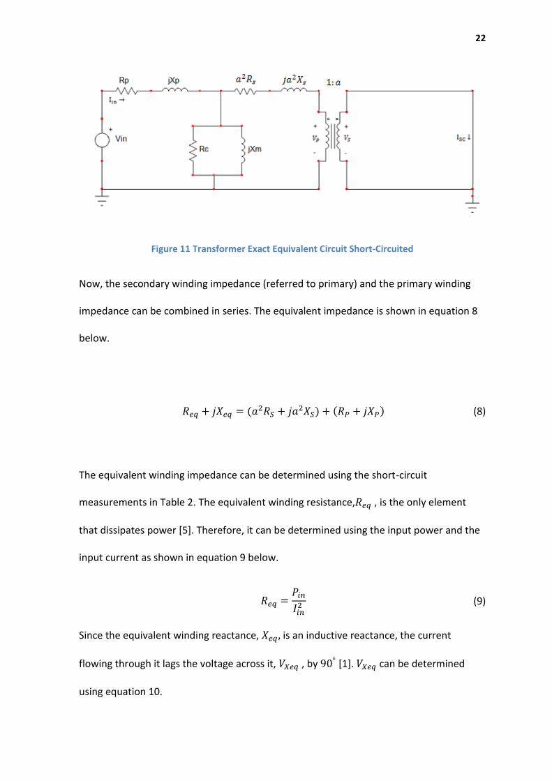
Figure 11 Transformer Exact Equivalent Circuit Short-Circuited

Now, the secondary winding impedance (referred to primary) and the primary winding

impedance can be combined in series. The equivalent impedance is shown in equation 8

below.

𝑅𝑒𝑞 + 𝑗𝑋𝑒𝑞 = (𝑎2𝑅𝑆 + 𝑗𝑎2𝑋𝑆) + (𝑅𝑃 + 𝑗𝑋𝑃) (8)

The equivalent winding impedance can be determined using the short-circuit

measurements in Table 2. The equivalent winding resistance,𝑅𝑒𝑞 , is the only element

that dissipates power [5]. Therefore, it can be determined using the input power and the

input current as shown in equation 9 below.

𝑅𝑒𝑞 =

𝑃𝑖𝑛

𝐼𝑖𝑛2 (9)

Since the equivalent winding reactance, 𝑋𝑒𝑞 , is an inductive reactance, the current

flowing through it lags the voltage across it, 𝑉𝑋𝑒𝑞 , by 90° [1]. 𝑉𝑋𝑒𝑞 can be determined

using equation 10.

23

𝑉𝑋𝑒𝑞 = √𝑉𝑖𝑛

2 − 𝑉𝑅𝑒𝑞2

(10)

Where, 𝑉𝑅𝑒𝑞 = 𝐼𝑖𝑛 𝑅𝑒𝑞 ,is the voltage across the equivalent winding resistance. 𝑋𝑒𝑞 can

now be determined using Ohm’s law as shown in equation 11 below.

𝑋𝑒𝑞 =

𝑉𝑋𝑒𝑞

𝐼𝑖𝑛

(11)

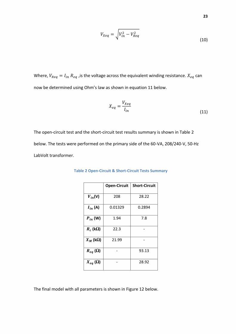
The open-circuit test and the short-circuit test results summary is shown in Table 2

below. The tests were performed on the primary side of the 60-VA, 208/240-V, 50-Hz

LabVolt transformer.

Table 2 Open-Circuit & Short-Circuit Tests Summary

Open-Circuit Short-Circuit

𝑽𝒊𝒏(V) 208 28.22

𝑰𝒊𝒏 (A) 0.01329 0.2894

𝑷𝒊𝒏 (W) 1.94 7.8

𝑹𝒄 (kΩ) 22.3 -

𝑿𝑴 (kΩ) 21.99 -

𝑹𝒆𝒒 (Ω) - 93.13

𝑿𝒆𝒒 (Ω) - 28.92

The final model with all parameters is shown in Figure 12 below.

24

Figure 12 Transformer Model

3.3 Voltage Regulation and Efficiency

These sets of experiments were carried out to test the transformer’s voltage regulation

and efficiency under various loading conditions in order to find the optimal load. Three

types of loads were used; resistive, inductive and capacitive. Each load type can be varied

from no-load to 4800 Ω to find the load with the maximum efficiency and minimum

voltage regulation [8]. The load is initially set to rated conditions (240 V, 0.25 A hence

𝑍𝐿=960 Ω). Figure 13 below shows the circuit connection for this experiment.

Figure 13 Voltage Regulation and Efficiency Experiment [7]

25

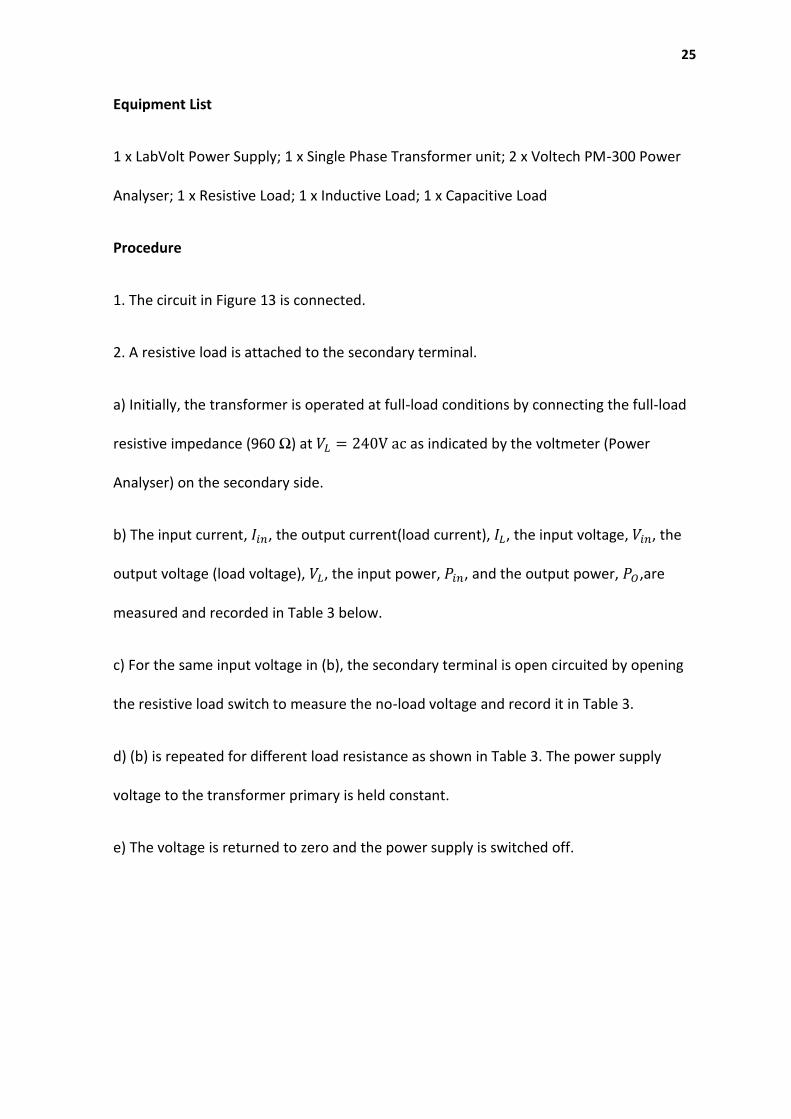
Equipment List


Analyser; 1 x Resistive Load; 1 x Inductive Load; 1 x Capacitive Load

Procedure

1. The circuit in Figure 13 is connected.

2. A resistive load is attached to the secondary terminal.

a) Initially, the transformer is operated at full-load conditions by connecting the full-load

resistive impedance (960 Ω) at 𝑉𝐿 = 240V ac as indicated by the voltmeter (Power

Analyser) on the secondary side.

b) The input current, 𝐼𝑖𝑛, the output current(load current), 𝐼𝐿, the input voltage, 𝑉𝑖𝑛, the

output voltage (load voltage), 𝑉𝐿, the input power, 𝑃𝑖𝑛, and the output power, 𝑃𝑂,are

measured and recorded in Table 3 below.

c) For the same input voltage in (b), the secondary terminal is open circuited by opening

the resistive load switch to measure the no-load voltage and record it in Table 3.

d) (b) is repeated for different load resistance as shown in Table 3. The power supply

voltage to the transformer primary is held constant.

e) The voltage is returned to zero and the power supply is switched off.

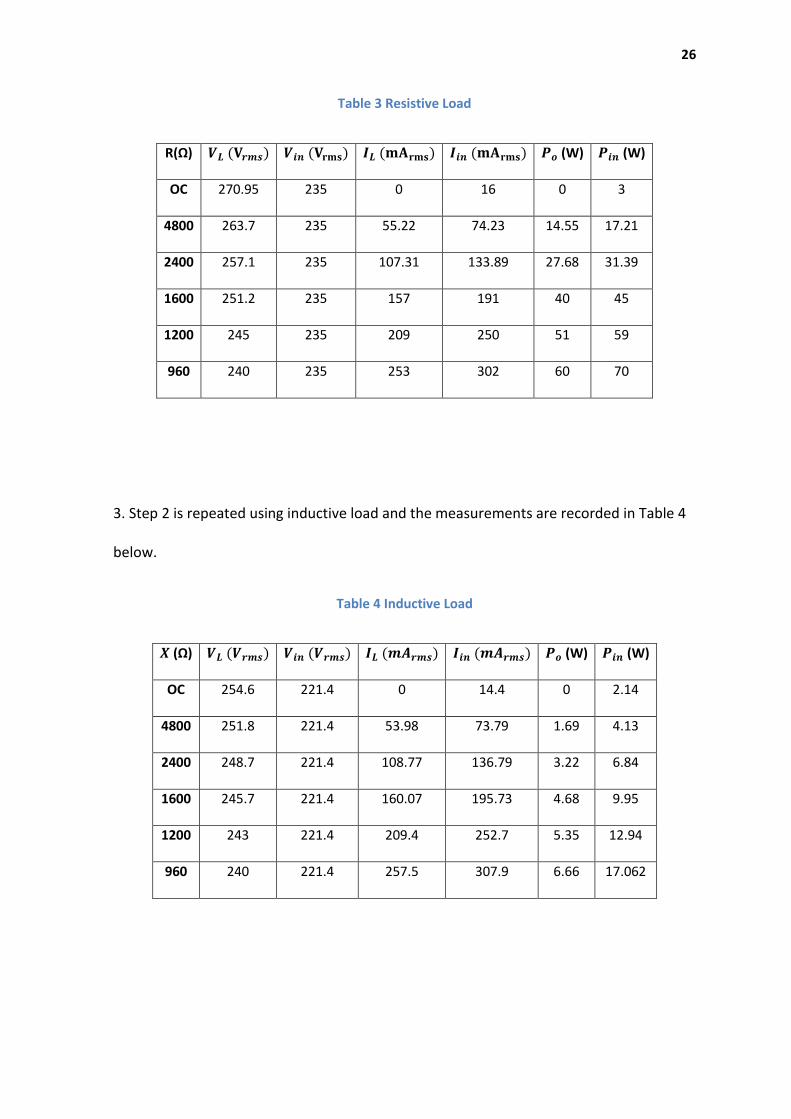
26

Table 3 Resistive Load

R(Ω) 𝑽𝑳 (𝐕𝒓𝒎𝒔) 𝑽𝒊𝒏 (𝐕𝐫𝐦𝐬) 𝑰𝑳 (𝐦𝐀𝐫𝐦𝐬) 𝑰𝒊𝒏 (𝐦𝐀𝐫𝐦𝐬) 𝑷𝒐 (W) 𝑷𝒊𝒏 (W)

OC 270.95 235 0 16 0 3

4800 263.7 235 55.22 74.23 14.55 17.21

2400 257.1 235 107.31 133.89 27.68 31.39

1600 251.2 235 157 191 40 45

1200 245 235 209 250 51 59

960 240 235 253 302 60 70

3. Step 2 is repeated using inductive load and the measurements are recorded in Table 4

below.

Table 4 Inductive Load

𝑿 (Ω) 𝑽𝑳 (𝑽𝒓𝒎𝒔) 𝑽𝒊𝒏 (𝑽𝒓𝒎𝒔) 𝑰𝑳 (𝒎𝑨𝒓𝒎𝒔) 𝑰𝒊𝒏 (𝒎𝑨𝒓𝒎𝒔) 𝑷𝒐 (W) 𝑷𝒊𝒏 (W)

OC 254.6 221.4 0 14.4 0 2.14

4800 251.8 221.4 53.98 73.79 1.69 4.13

2400 248.7 221.4 108.77 136.79 3.22 6.84

1600 245.7 221.4 160.07 195.73 4.68 9.95

1200 243 221.4 209.4 252.7 5.35 12.94

960 240 221.4 257.5 307.9 6.66 17.062

27

4. Step 2 is repeated using capacitive load and the measurements are recorded in Table 5

below.

Table 5 Capacitive Load

𝑿 (Ω) 𝑽𝑳 (𝑽𝒓𝒎𝒔) 𝑽𝒊𝒏 (𝑽𝒓𝒎𝒔) 𝑰𝑳 (𝒎𝑨𝒓𝒎𝒔) 𝑰𝒊𝒏 (𝒎𝑨𝒓𝒎𝒔) 𝑷𝒐 (mW) 𝑷𝒊𝒏 (W)

OC 232.7 202.4 0 12.96 0 1.86

4800 234.4 202.4 49.91 50.13 133 2.13

2400 236.1 202.4 100.39 107.78 103 2.98

1600 237.4 202.4 149.55 164.48 135 4.49

1200 238.6 202.4 197 219.2 108 6.39

960 240 202.4 247.2 276.8 115 9.1

Now, the Tables above can be used to calculate the voltage regulation for each load type

as shown in equation 12 below.

𝑉𝑅 =

𝑉𝑁𝐿 − 𝑉𝐹𝐿

𝑉𝑁𝐿 × 100%

(12)

The voltage regulation is calculated for each load type as shown in Table 6 below.

28

Table 6 Voltage Regulation

The transformer efficiency for different impedance values in each load type can be also

calculated from Tables (3-5) above using equation 13.

𝜂 =

𝑃𝑂

𝑃𝑖𝑛 × 100%

(13)

Where, 𝑃𝑂 is the output power (delivered to load) and 𝑃𝑖𝑛 is the input power from the

power supply.

Table 7 Efficiency for Each Load Type at Variable Impedance

Impedance (Ω) Resistive (%) Inductive (%) Capacitive (%)

4800 84.54 40.92 6.24

2400 88.18 47.03 3.01

1600 88.89 47.08 3.46

1200 86.44 41.13 1.69

960 85.71 39.03 1.26

Figure 14 below shows the regulation curve for each load type.

Load VR%

Resistive 11.42

Inductive 5.734

Capacitive -3.137

29

Figure 14 Regulation Curves

Observations

It can be seen from Tables (3-5) that a practical transformer’s output voltage is affected

by load variation. Voltage regulation measures the change in the output voltage due to

load variations [5].

From Table 6, the transformer has the worst voltage regulation when the resistive load is

used. The capacitive load gives a negative voltage regulation because the no-load voltage

is lower than the full-load voltage.

The inductive load has a higher efficiency than the capacitive load due to resistance in the

inductive load which makes it consume more active power [2]. In other words, the

inductive load is not ideal and has some resistance in it.

3.4 Winding Resistance Segregations

The winding resistance and leakage reactance found from the short-circuit test are the

equivalent values of the primary and secondary side referred to the primary side.

230

235

240

245

250

255

260

265

270

275

0 100 200 300

Load

Vo

ltag

e (

V)

Load Current (mA)

Regulation Curves

Resistive Load

Capacitive Load

Inductive Load

30

Therefore, this experiment was carried out in order to find the separate values of 𝑅𝑃 and

𝑅𝑆.

Since the transformer is available in the laboratory, 𝑅𝑃 and 𝑅𝑆 were measured directly

using a digital multi meter (DMM). 𝑅𝑃 and 𝑅𝑆 were also experimentally determined by

energizing one side of the transformer while the other is open-circuited or short

circuited. A dc power supply was used to energize the transformer to eliminate the effect

of the leakage reactance in this experiment.

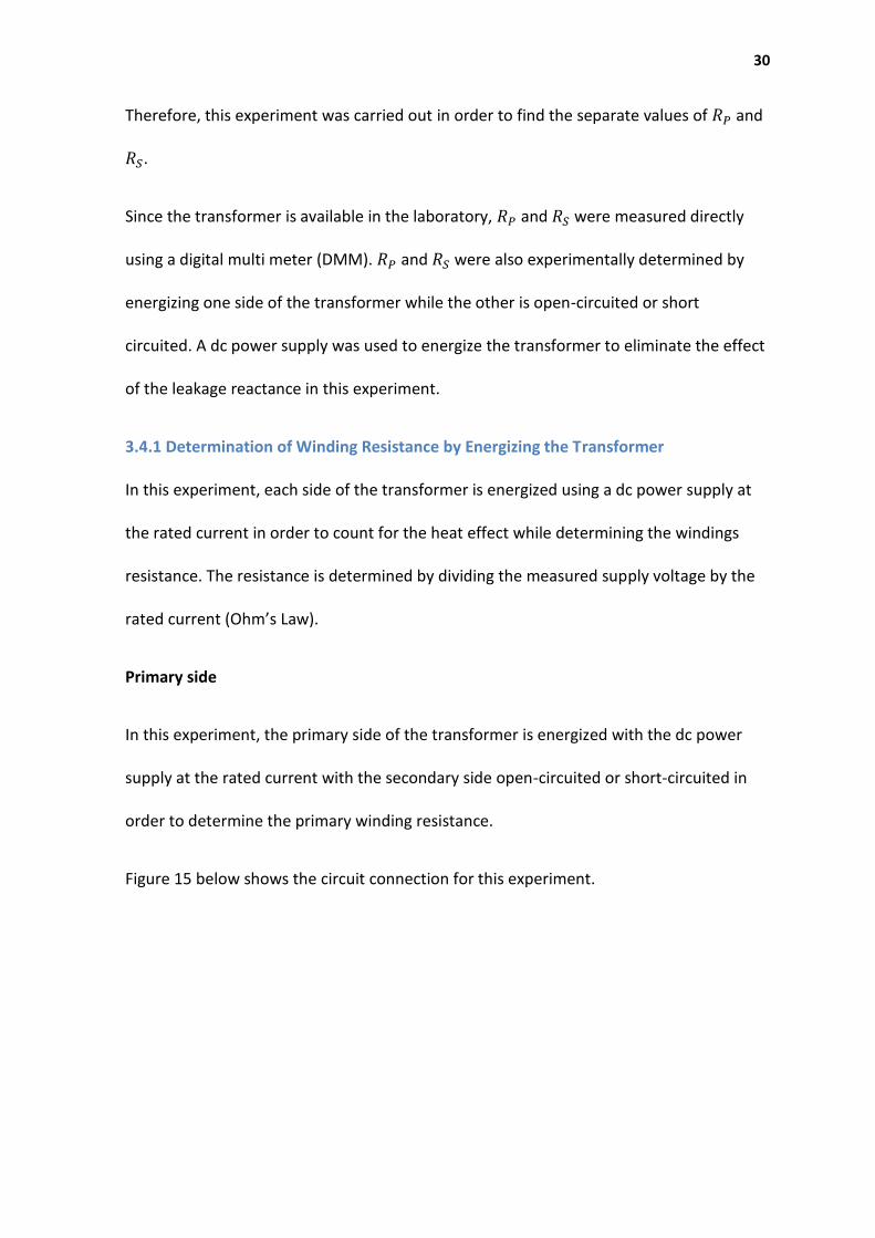
3.4.1 Determination of Winding Resistance by Energizing the Transformer

In this experiment, each side of the transformer is energized using a dc power supply at

the rated current in order to count for the heat effect while determining the windings

resistance. The resistance is determined by dividing the measured supply voltage by the

rated current (Ohm’s Law).

Primary side

In this experiment, the primary side of the transformer is energized with the dc power

supply at the rated current with the secondary side open-circuited or short-circuited in

order to determine the primary winding resistance.

Figure 15 below shows the circuit connection for this experiment.

31

Figure 15 Primary Winding Resistance Measurement Under Open-circuit Conditions [7]

In Figure 15 above, measurements of the supply voltage and current are taken on the

primary side with the secondary side open-circuited.

Equipment List

1 x LabVolt Power Supply (dc); 1 x Single Phase Transformer unit; 1 x VolTech PM-300

Power Analyser

Procedure


2. The power supply is switched on and the input voltage is increased until the rated

winding current is reached (0.15A) as indicated by the ammeter 𝐼𝑖𝑛.

3. The input voltage, input current are measured and recorded in Table 8.


32

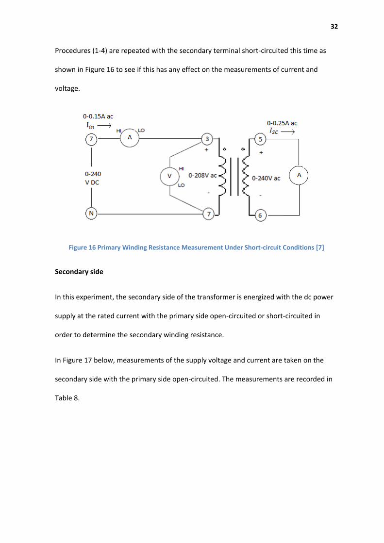
Procedures (1-4) are repeated with the secondary terminal short-circuited this time as

shown in Figure 16 to see if this has any effect on the measurements of current and

voltage.

Figure 16 Primary Winding Resistance Measurement Under Short-circuit Conditions [7]

Secondary side

In this experiment, the secondary side of the transformer is energized with the dc power

supply at the rated current with the primary side open-circuited or short-circuited in

order to determine the secondary winding resistance.

In Figure 17 below, measurements of the supply voltage and current are taken on the

secondary side with the primary side open-circuited. The measurements are recorded in

Table 8.

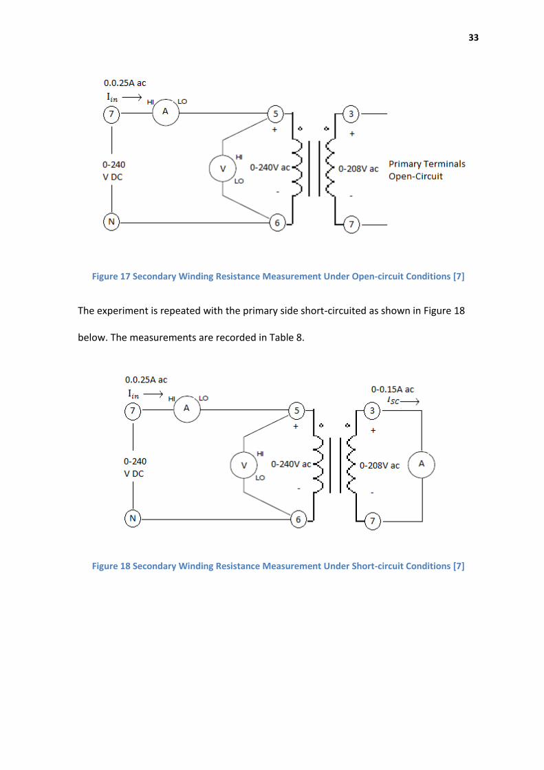
33

Figure 17 Secondary Winding Resistance Measurement Under Open-circuit Conditions [7]

The experiment is repeated with the primary side short-circuited as shown in Figure 18

below. The measurements are recorded in Table 8.

Figure 18 Secondary Winding Resistance Measurement Under Short-circuit Conditions [7]

34

Table 8 Winding Resistance Segregation

Excitation side Primary Side Energized Secondary Side Energized

Measurements 𝑰𝒊𝒏 (𝒎𝑨𝒓𝒎𝒔) 𝑽𝒊𝒏 (𝑽𝒓𝒎𝒔) 𝑹𝒑 (Ω) 𝑰𝒊𝒏 (𝒎𝑨𝒓𝒎𝒔) 𝑽𝒊𝒏 (𝑽𝒓𝒎𝒔) 𝑹𝒔 (Ω)

Open-Circuit 0.15 9.84 65.6 0.25 10 40

Short-Circuit 0.15 9.5 63.33 0.25 9.9 39.6

Observations

It can be seen from Table 8 that the open-circuited or short-circuited side of the

transformer has a negligible effect on the energized side where measurements of current

and voltage are taken. Values of 𝑅𝑝 and 𝑅𝑠 are very close under open-circuit and short-

circuit conditions. Therefore, it does not really matter whether one side of the

transformer is open-circuited or short-circuited while taking measurements on the other

(energized) side.

The equivalent value of the windings resistance referred to the primary side obtained

from the short-circuit test in Table 1 (𝑅𝑒𝑞) is close to the equivalent value of 𝑅𝑝 and 𝑅𝑠 in

Table 8 above. The short-circuit test is found to be accurate enough to estimate the

equivalent resistance of the windings. Therefore, the 𝑅𝑒𝑞 value (93.13 Ω) was used in the

simulated model.

3.4.2 Measuring the Windings Resistance Using DMM

The resistance across the primary and secondary windings was measured in the

laboratory directly using a digital multi meter. The measured values are as follows;

𝑅𝑝 = 61 𝑂ℎ𝑚𝑠, 𝑅𝑠 = 37.8 𝑂ℎ𝑚𝑠 which gives an equivalent value referred to the primary

35

side of 89.39. This is a bit lower than the values in Table 1 and Table 8. This method is less

accurate because of the heat effect that appears when the transformer is energized at

the rated windings current.

36

4.0 Simulations

After finding the model parameters from the experimental measurements (see Figure

11), several simulations were run to verify the experimental results.

4.1 No-Load Voltage

These simulations were run to verify which load type gives the highest no-load voltage.

The transformer is operated at full-load conditions (𝑉𝐿 = 240V ac, 𝐼𝐿 = 0.25A ac, 𝑍𝐿 =

960 Ω). The secondary terminal is then open-circuited to measure the no-load voltage.

The input data is summarized in Table 9 below.

Table 9 No-Load Simulation Input Data

Input Data Resistive Load Inductive Load Capacitive Load

𝑽𝒊𝒏 (𝑽𝒓𝒎𝒔) 236.07 219.91 286

𝑹𝒆𝒒 (Ω) 93.13 93.13 93.13

𝑳𝒆𝒒 (H) 0.092 0.092 0.092

𝑹𝒄 (kΩ) 22.3 22.3 22.3

𝑳𝒎 (H) 70 70 70

Transformer Ratio 208/240 208/240 208/240

Frequency (Hz) 50 50 50

𝒁𝑳 960 Ω 3.057 H 3.23 µF

The simulation results agreed with the experimental measurements as shown in Table 10

below. The output voltages are listed for both full-load (960 Ω) and no-load conditions.

37

Table 10 No-Load Voltage Simulation Results

Load Resistive Load Inductive Load Capacitive Load

960 (Ω)

Experimental

239.93 V

240 V

240.1 V

240 V

240.04 V

240V

OC

Experimental

270.95 V

270.95 V

252.29 V

254.6 V

232 V

232.7 V

4.2 Voltage Regulation and Efficiency Simulations

This set of simulations was run to find out the voltage regulation and efficiency for each

load type at variable impedance. The simulation results will be compared with

experimental results. The input data is the same as in Table 9, but the load impedance

will be varied from no load to 4800 Ω. Tables (11-13) summarize the simulation results

for each load type.

Table 11 Resistive Load Simulation Results

R

(Ω)

𝑽𝑳

(𝑽𝒓𝒎𝒔)

𝑽𝒊𝒏

(𝑽𝒓𝒎𝒔)

𝑰𝑳

(𝒎𝑨𝒓𝒎𝒔)

𝑰𝒊𝒏


𝑷𝒐

(W)

𝑷𝒊𝒏

(W)

VR

(%)

𝜼

(%)

OC 270.95 236.071 0 19.87 0 3

11.45

0

4800 264.15 236.071 55.03 75.78 15 18 83.33

2400 257.66 236.071 107.36 135.078 27.66 31.65 87.39

1600 251.47 236.071 157.17 192 40 45 88.89

1200 245.57 236.071 204.64 246.39 50 58 86.21

960 239.93 236.071 249.93 298.33 60 70 85.71

38

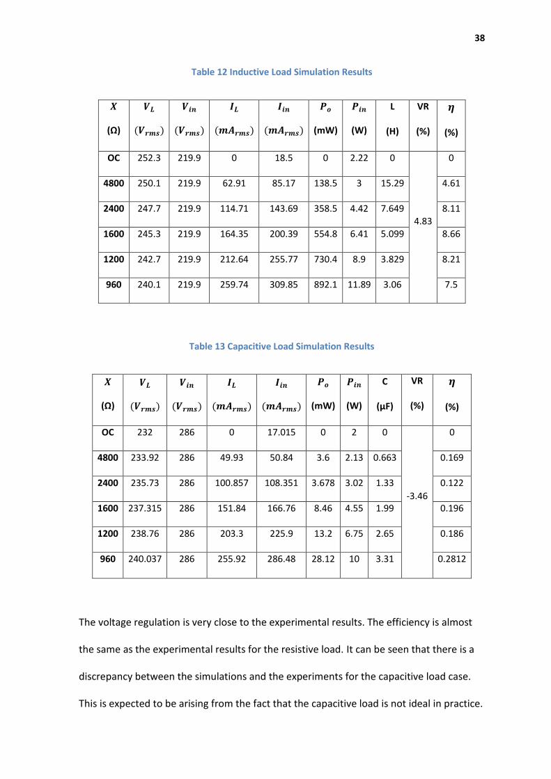
Table 12 Inductive Load Simulation Results

𝑿

(Ω)

𝑽𝑳

(𝑽𝒓𝒎𝒔)

𝑽𝒊𝒏

(𝑽𝒓𝒎𝒔)

𝑰𝑳


𝑰𝒊𝒏


𝑷𝒐

(mW)

𝑷𝒊𝒏

(W)

L

(H)

VR

(%)

𝜼

(%)

OC 252.3 219.9 0 18.5 0 2.22 0

4.83

0

4800 250.1 219.9 62.91 85.17 138.5 3 15.29 4.61

2400 247.7 219.9 114.71 143.69 358.5 4.42 7.649 8.11

1600 245.3 219.9 164.35 200.39 554.8 6.41 5.099 8.66

1200 242.7 219.9 212.64 255.77 730.4 8.9 3.829 8.21

960 240.1 219.9 259.74 309.85 892.1 11.89 3.06 7.5

Table 13 Capacitive Load Simulation Results

𝑿

(Ω)

𝑽𝑳

(𝑽𝒓𝒎𝒔)

𝑽𝒊𝒏

(𝑽𝒓𝒎𝒔)

𝑰𝑳


𝑰𝒊𝒏


𝑷𝒐

(mW)

𝑷𝒊𝒏

(W)

C

(µF)

VR

(%)

𝜼

(%)

OC 232 286 0 17.015 0 2 0

-3.46

0

4800 233.92 286 49.93 50.84 3.6 2.13 0.663 0.169

2400 235.73 286 100.857 108.351 3.678 3.02 1.33 0.122

1600 237.315 286 151.84 166.76 8.46 4.55 1.99 0.196

1200 238.76 286 203.3 225.9 13.2 6.75 2.65 0.186

960 240.037 286 255.92 286.48 28.12 10 3.31 0.2812

The voltage regulation is very close to the experimental results. The efficiency is almost

the same as the experimental results for the resistive load. It can be seen that there is a

discrepancy between the simulations and the experiments for the capacitive load case.

This is expected to be arising from the fact that the capacitive load is not ideal in practice.

39

Moreover, the inductive load gave significantly lower values of efficiency in the

simulations. This may be due to the resistance in the inductive load (in the experiment).

Therefore, this inductive load can be modelled by a resistor in series with an ideal

inductor and repeating the simulation. The resistance across each inductive load was

measured and taken into account in the simulation. Table 14 shows the simulation results

after adding the resistance to an ideal inductive load.

Table 14 Simulation results after modelling an inductive load using an ideal inductor in series

with a resistor

Inductive+R 𝑽𝑳(𝑽𝒓𝒎𝒔) 𝑷𝒊𝒏 (W) 𝑷𝒐 (W) Efficiency (%) 𝑹𝑳Measured (Ω)

4800 240.39 1.73 0.47 27.40 269

2400 239.96 2.79 0.98 35.21 147

1600 240.65 4.12 1.42 34.56 95

1200 240.14 5.67 1.79 31.62 68

960 240.27 7.58 2.21 29.10 54

40

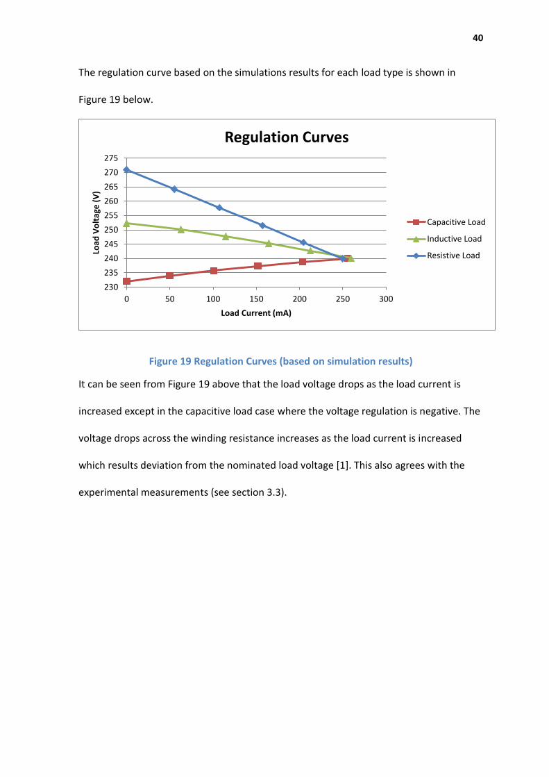
The regulation curve based on the simulations results for each load type is shown in

Figure 19 below.

Figure 19 Regulation Curves (based on simulation results)

It can be seen from Figure 19 above that the load voltage drops as the load current is

increased except in the capacitive load case where the voltage regulation is negative. The

voltage drops across the winding resistance increases as the load current is increased

which results deviation from the nominated load voltage [1]. This also agrees with the

experimental measurements (see section 3.3).

230

235

240

245

250

255

260

265

270

275

0 50 100 150 200 250 300

Load

Vo

ltag

e (

V)

Load Current (mA)

Regulation Curves

Capacitive Load

Inductive Load

Resistive Load

41

5.0 Maximum Efficiency Criterion

Equation 13 can be rewritten in a more detailed form that indicates power losses as

shown in equation 14 below.

𝜂 =

𝑎𝑉𝐿𝐼𝐿𝑃𝐹

𝑎𝑉𝐿𝐼𝐿𝑃𝐹 + 𝑃𝑚 + 𝐼𝐿2𝑅𝑒𝑞

× 100%

(14)

Where 𝑎 is the transformer’s turns ratio, 𝑉𝐿 is the load voltage, 𝐼𝐿 is the load current, PF is

the power factor, 𝑃𝑚 is the core loss, 𝑅𝑒𝑞is the equivalent winding resistance referred to

primary side.

The core loss is fixed regardless of variations in the load [1]. 𝑃𝑚 is measured as the input

power in the open-circuit test . This is because the magnetization element is dissipating

all the input power in this case [1]. The copper loss, on the other hand, is proportional to

the current flowing through the winding [1].

The efficiency increases as the load increases up to a certain value after which it starts

going down [1]. The load current at the maximum efficiency is given by equation 15

below [1].

𝐼𝐿𝜂 = √

𝑃𝑚

𝑅𝑒𝑞

(15)

42

The efficiency is calculated using equation 14 at load currents of (20 per cent-100 per

cent) of the rated value with all other variables fixed at rated conditions with a power

factor of 0.8. A plot of efficiency against load current is shown in Figure 20 below.

Figure 20 Efficiency vs Load Current

The efficiency reaches its maximum when the copper loss equals the core loss [3]. This is

shown in Figure 21 below. The percentage load current and the copper loss are based on

the load current measurements in Table 3 (Resistive Load). Figure 21 shows that copper

losses equals core losses at around 60 per cent load current, which implies that the

maximum efficiency is at about 60 per cent of the rated load current.

This corresponds to a load impedance of 1600 Ω. In the experimental results and the

simulation results, the maximum efficiency was observed at this load impedance (see

Table 7, Table 11, Table 12 and Table 13).

43

Figure 21 Load Current at Maximum Efficiency

From equation 14, the power factor also affects the efficiency. Therefore, the efficiency

at a power factor ranging from (0.5-1) with all other variables fixed at rated conditions is

plotted in Figure 22 below.

Figure 22 Efficiency against PF

81

82

83

84

85

86

87

88

89

90

91

0.5 0.6 0.7 0.8 0.9 1 1.1

Effi

cie

ncy

(%)

PF

Efficiency vs PF

Efficiency

44

6.0 Sensitivity Analysis

A sensitivity analysis is carried out on the efficiency to the electrical parameters as well as

the design parameters. The relationship between power losses and the associated design

parameters is discussed. A mathematical model that directly relates the design

parameters to the efficiency is then developed.

6.1 Electrical Parameters

In this section, each of the model parameters is varied by ± 10 per cent of its value to see

the effect of such variations on the transformer’s performance at full load conditions.

This sensitivity analysis is based on the simulated model using ICAPS. Tables (15-22) show

the transformer’s behaviour in response to variations in each of the model parameters.

6.1.1 Core-loss Resistance (𝑹𝒄)

The core resistance 𝑅𝑐 is varied by 10 per cent higher and lower than the original value in

the complete equivalent circuit (see Figure 10). First, 𝑅𝑐 is increased by 10 per cent which

brings it to 24.53 kΩ. 𝑅𝑐 is associated with the core loss which can be determined by the

open-circuit test. It is inversely proportional to the core-loss current [2]. Therefore, it is

mainly the input power that will be tracked in this simulation as it represents the core-

loss (no-load loss) under open-circuit conditions.

The results for this simulation at no-load conditions are summarized in Table 15 below.

45

Table 15 Core-Loss Resistance 10% Increase

Original Value 10% Increase

𝑹𝒄 → 22.3kΩ 24.53kΩ

𝑽𝑳 (𝐕𝒓𝒎𝒔) 270.95 271.016

𝑽𝒊𝒏 (𝐕𝒓𝒎𝒔) 236.071 236.071

𝑰𝒊𝒏 (mArms) 19.87 19.39

𝑷𝒊𝒏(W) 2.565 2.34

It can be seen from Table 15 above that increasing 𝑅𝑐 by 10 per cent leads to 8.59 per

cent decrease in 𝑃𝑖𝑛 which means the core-loss is reduced. This is expected as the eddy

current loss component of the core-loss is inversely proportional to 𝑅𝑐. Therefore, the

transformer’s efficiency improves if it is designed to have low core-loss resistance

Now, 𝑅𝑐 is reduced by 10 per cent this time and the simulation results are recorded in

Table 16 below.

Table 16 Core-Loss Resistance 10% Decrease

Original Value 10% Decrease

𝑹𝒄 → 22.3kΩ 20.07kΩ

𝑽𝑳 (𝐕𝒓𝒎𝒔) 270.95 270.788

𝑽𝒊𝒏 (𝐕𝒓𝒎𝒔) 236.071 236.071

𝑰𝒊𝒏 (mArms) 19.87 20.53

𝑷𝒊𝒏(W) 2.565 2.84

46

Reducing 𝑅𝑐 by 10 per cent, on the other hand, leads to increased core-loss by 10.72 per

cent of the original value.

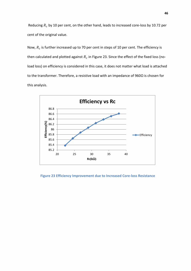
Now, 𝑅𝑐 is further increased up to 70 per cent in steps of 10 per cent. The efficiency is

then calculated and plotted against 𝑅𝑐 in Figure 23. Since the effect of the fixed loss (no-

load loss) on efficiency is considered in this case, it does not matter what load is attached

to the transformer. Therefore, a resistive load with an impedance of 960Ω is chosen for

this analysis.

Figure 23 Efficiency Improvement due to Increased Core-loss Resistance

85.2

85.4

85.6

85.8

86

86.2

86.4

86.6

86.8

20 25 30 35 40

Effi

cie

ncy

(%)

Rc(kΩ)

Efficiency vs Rc

Efficiency

47

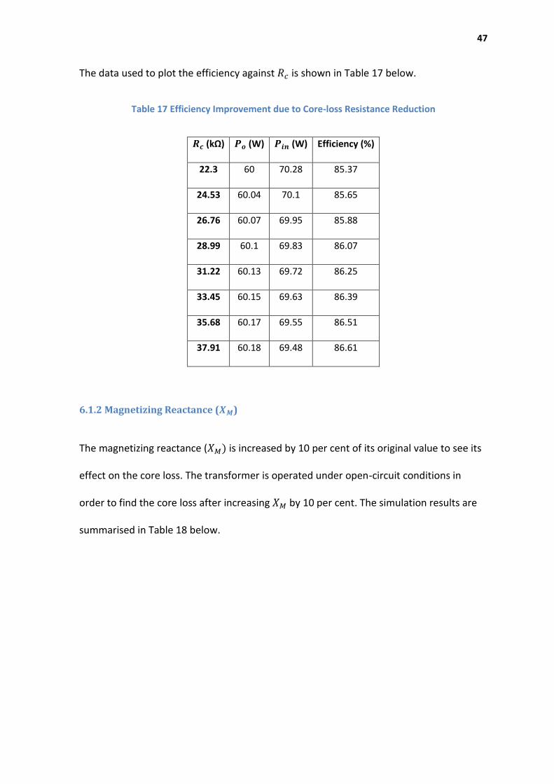
The data used to plot the efficiency against 𝑅𝑐 is shown in Table 17 below.

Table 17 Efficiency Improvement due to Core-loss Resistance Reduction

𝑹𝒄 (kΩ) 𝑷𝒐 (W) 𝑷𝒊𝒏 (W) Efficiency (%)

22.3 60 70.28 85.37

24.53 60.04 70.1 85.65

26.76 60.07 69.95 85.88

28.99 60.1 69.83 86.07

31.22 60.13 69.72 86.25

33.45 60.15 69.63 86.39

35.68 60.17 69.55 86.51

37.91 60.18 69.48 86.61

6.1.2 Magnetizing Reactance (𝑿𝑴)

The magnetizing reactance (𝑋𝑀) is increased by 10 per cent of its original value to see its

effect on the core loss. The transformer is operated under open-circuit conditions in

order to find the core loss after increasing 𝑋𝑀 by 10 per cent. The simulation results are

summarised in Table 18 below.

48

Table 18 Magnetizing Reactance 10% Increase


𝑿𝑴 → 21.99kΩ 24.189kΩ

𝑽𝑳 (𝐕𝒓𝒎𝒔) 270.95 270.979

𝑽𝒊𝒏 (𝐕𝒓𝒎𝒔) 236.071 236.105

𝑰𝒊𝒏 (mArms) 19.87 18.698

𝑷𝒊𝒏(W) 2.565 2.561

Increasing 𝑋𝑀 by 10 per cent has a negligible effect on the input power which represents

the core loss in this case.

6.1.3 Equivalent Winding Resistance (𝑹𝒆𝒒)

Similarly, the equivalent winding resistance (𝑅𝑒𝑞) is varied by 10 per cent to see its effect

on the transformer’s performance. 𝑅𝑒𝑞 is associated with the copper loss which is load-

dependent. Therefore, the simulation is run under full-load conditions to observe the

maximum copper loss. 𝑅𝑒𝑞 is increased by 10 per cent and the simulation results are


Table 19 Winding Resistance 10% Increase


𝑹𝒆𝒒 → 93.13Ω 102.443Ω

𝑽𝑭𝑳 (𝐕𝒓𝒎𝒔) 239.93 237.151

𝑽𝑵𝑳 (𝐕𝒓𝒎𝒔) 270.95 270.798

𝑽𝑹 % 11.44 12.43

49

It can be seen from Table 19 that the voltage regulation (VR) has increased by 8.65 per

cent of its original value after increasing the equivalent winding resistance by 10 per cent.

This is expected because the higher the winding resistance, the higher the voltage drops

lost across it.

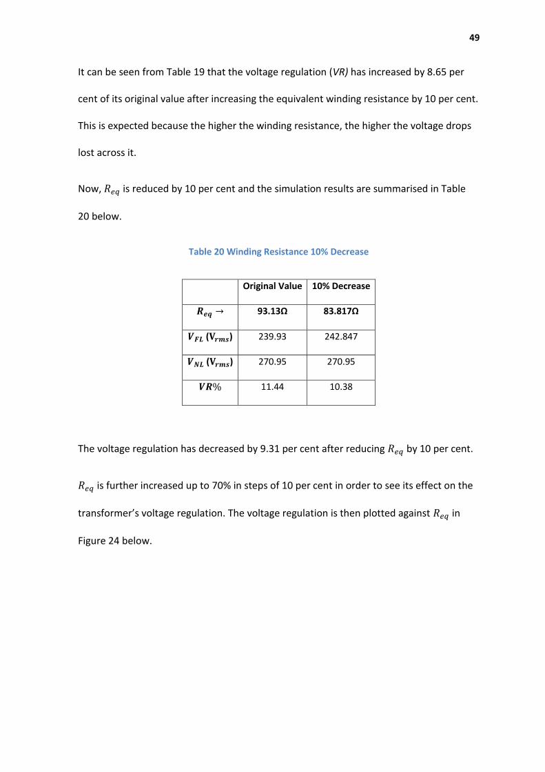
Now, 𝑅𝑒𝑞 is reduced by 10 per cent and the simulation results are summarised in Table

20 below.

Table 20 Winding Resistance 10% Decrease

Original Value 10% Decrease

𝑹𝒆𝒒 → 93.13Ω 83.817Ω

𝑽𝑭𝑳 (𝐕𝒓𝒎𝒔) 239.93 242.847

𝑽𝑵𝑳 (𝐕𝒓𝒎𝒔) 270.95 270.95

𝑽𝑹% 11.44 10.38

The voltage regulation has decreased by 9.31 per cent after reducing 𝑅𝑒𝑞 by 10 per cent.

𝑅𝑒𝑞 is further increased up to 70% in steps of 10 per cent in order to see its effect on the

transformer’s voltage regulation. The voltage regulation is then plotted against 𝑅𝑒𝑞 in

Figure 24 below.

50

Figure 24 Increased Voltage Regulation due to Variations in the Equivalent Winding Resistance

The analysis data used to plot the voltage regulation against 𝑅𝑒𝑞 is shown in Table 21

below.

Table 21 Increased Voltage Regulation due to Increase in the Equivalent Winding Resistance

𝑹𝒆𝒒(Ω) 𝑽𝑵𝑳 (𝐕𝒓𝒎𝒔) 𝑽𝑭𝑳 (𝐕𝒓𝒎𝒔) 𝑽𝑹%

93.13 239.93 270.95 11.44

102.44 237.15 270.798 12.43

111.76 234.49 270.726 13.38

121.07 231.83 270.61 14.33

130.38 229.23 270.495 15.25

139.69 226.69 270.38 16.16

149.01 224.2 270.265 17.04

158.321 221.77 270.15 17.90857

11

12

13

14

15

16

17

18

19

90 110 130 150 170

VR

(%)

Req(Ω)

Voltage Regulation vs Req

Voltage Regulation

51

It can be seen that the voltage regulation is highly sensitive to variations in 𝑅𝑒𝑞. The

voltage regulation has increased by 56.56 per cent of its original value.

6.1.4 Equivalent Leakage Reactance (𝑿𝒆𝒒)

In this section, the voltage regulation is also traced against variations in the equivalent

leakage reactance. 𝑋𝑒𝑞 is increased by 10 per cent and the simulation results are


Table 22 Leakage Reactance 10% Increase


𝑿𝒆𝒒 → 28.92 Ω 31.81 Ω

𝑽𝑭𝑳 (𝐕𝒓𝒎𝒔) 239.93 239.866

𝑽𝑵𝑳 (𝐕𝒓𝒎𝒔) 270.95 270.869

𝑽𝑹 % 11.44 11.45

The change in the voltage regulation due to 10 per cent increase in 𝑋𝑒𝑞 is only 0.09 per

cent of the original value which is quite negligible.

The simulations indicated that the transformer’s performance is most sensitive to the

windings equivalent resistance which is proportional to the copper loss. This is expected

as copper loss is in turn proportional to the voltage regulation [1]

6.2 Physical Design Parameters

In this section, the design parameters that can be optimized in order to reduce the losses

and therefore improve the efficiency are considered.

52

6.2.1 Core losses

A well designed transformer core is meant to have a low reluctance path for the magnetic

flux linking the primary and secondary windings. The core has hysteresis and eddy

currents due to iron losses in the form of heat. The alternating flux also can generate un-

tolerated noise especially in large transformers. Therefore, reduction of noise is another

concern besides loss reduction for transformer designers [3]. This project, however, is

only focused on loss reduction in order to maximise efficiency.

There are two types of core loss: the hysteresis loss which is proportional to the

frequency of operation, the volume of the material and the hysteresis loop area [9]. The

area of a hysteresis loop is determined by the magnetic characteristics of the core

material. Specifically, it is the peak flux density of the core material that determines the

hysteresis loop area. The other type of core loss is the eddy current loss which is

dependent on the square of frequency of operation. The thickness of the core material is

also a major factor which determines the eddy current loss [3]. Consequently, a well-

designed transformer core is made of a material having a minimum area of hysteresis

loop, thin laminations and high material resistivity in order to minimise eddy current and

hysteresis loss.

Hysteresis loss is given by equation 16 and eddy current loss is represented by equation

17 below [10].

𝑃ℎ = 2.2𝑘ℎ𝑓𝐵𝑚𝑎𝑥𝑛 (W/kg)

(16)

53

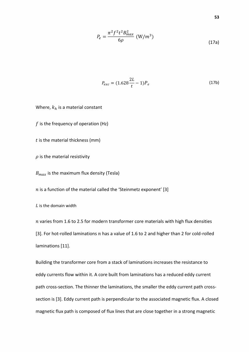
𝑃𝑒 =

𝜋2𝑓2𝑡2𝐵𝑚𝑎𝑥2

6𝜌 (W/𝑚3)

(17a)

𝑃𝑒𝑥𝑐 = (1.628

2𝐿

𝑡− 1)𝑃𝑒 (17b)

Where, 𝑘ℎ is a material constant

𝑓 is the frequency of operation (Hz)

𝑡 is the material thickness (mm)

𝜌 is the material resistivity

𝐵𝑚𝑎𝑥 is the maximum flux density (Tesla)

𝑛 is a function of the material called the ‘Steinmetz exponent’ [3]

𝐿 is the domain width

𝑛 varies from 1.6 to 2.5 for modern transformer core materials with high flux densities

[3]. For hot-rolled laminations 𝑛 has a value of 1.6 to 2 and higher than 2 for cold-rolled

laminations [11].

Building the transformer core from a stack of laminations increases the resistance to

eddy currents flow within it. A core built from laminations has a reduced eddy current

path cross-section. The thinner the laminations, the smaller the eddy current path cross-

section is [3]. Eddy current path is perpendicular to the associated magnetic flux. A closed

magnetic flux path is composed of flux lines that are close together in a strong magnetic

54

field and further apart in a weak one [12]. In the case of a laminated core, the flux lines

are further apart which makes it harder for eddy current to flow.

It can be seen from the eddy current loss equation above that it is composed of two

components: the first is called the classical eddy current loss which is dependent on the

square of frequency times material thickness times flux density (from equation 17a

above); the second component is the residual loss (excess eddy current loss) which is

dependent on the material structure such as the magnetic domain movement during the

magnetizing cycle. The relationship between classical eddy current loss and excess eddy

current loss is given by equation 17b [13]. The residual loss forms half of the total steel

loss, which is a significant proportion. Therefore, it is the residual that is significantly

reduced by special processing of the core material [3]. There is a wide range of

conventionally rolled core steels processed in a way such that core-loss is minimized. A

few types of these core materials will be considered in this project to see variations in the

eddy current loss and the hysteresis loss.

As mentioned earlier, the thinner the laminations the lower the core loss. However,

cutting the laminations into thinner sheets causes the appearance of some strains that

increase the core loss [1]. Therefore, the laminations are exposed to high temperatures

to remove the strains in the annealing process. Moreover, the magnetic losses are

reduced by adding materials to the iron such as silicon or aluminium [3]. Different

technologies used in core loss reduction are considered below.

55

Hot-rolled steel

Adding silicon to the core material reduces the area of the hysteresis loop. Moreover, it

reduces eddy current loss as it increases the core’s resistivity and permeability. However,

the quantity of the added silicon is limited to 4.5 per cent of the material because adding

too much silicon makes the core too brittle for the manufacture process. Silicon also has

the advantage of carbon elimination, which significantly reduces the core loss [3].

Purified core materials have substantially lower losses. For example, the first steel-silicon

manufactured had a specific loss of 7 W/kg at 1.5 Tesla and 50 Hz. In 1990, alloys at the

same conditions (1.5 Tesla and 50 Hz) with higher purity levels have losses of 2 W/kg [3].

Since steel sheets characterize a crystalline structure (grains), their magnetic properties

depend on the measurement direction in those individual grains [3]. In hot-rolled steel,

the grains are packed randomly. Therefore, the measured magnetic properties in this

kind of sheet are the average of values for different measurement directions. This kind of

material is called isotropic [3].

Grain-oriented (cold-rolled) steel

Once it was realized that silicon steel crystals are anisotropic, the orientation of the steel

crystal had been taken into account to optimize the magnetization in the core [3]. In this

kind of steel, the grains are aligned within ±6°of the rolling direction (ideal Goss

orientation) which reduces the hysteresis loss component in the core [3]. The thickness of

grain-oriented steel is reduced to 0.28 mm which reduces the classical eddy current loss.

Hysteresis loss is the heat energy lost on each cycle. The hysteresis loop represents the

volumetric energy converted to heat each cycle. Therefore, the higher the frequency of

56

operation, the more power lost due to hysteresis. In transformers, heat energy loss is not

desirable unlike other magnetic circuits such as permanent magnets. Therefore, a well-

designed transformer should have a core made of an alloy having a thin hysteresis loop.

In other words, the core should have a small residual flux density which results in a

thinner hysteresis loop [6].

In practice, there are other factors affecting core-loss that are not considered in this

project. This includes poorly insulated core laminations, improper handling of the core

steel during the manufacture process and poorly arranged core joints. These are

modelled by the building factor which is a ratio of the experimentally measured core-loss

to the core-loss nominated by the manufacturer [7].

The American Iron and Steel Institute (AISI) designates electrical steel types by the letter

M (magnetic material) followed by the type number [14].

Core loss sensitivity analysis

A sensitivity analysis is carried out using equations 16 and 17. Each of the design

parameters is varied while keeping all other parameters constant for a particular core

material. The material used for this analysis is non-oriented electrical steel as shown in

Table 23 below [15].

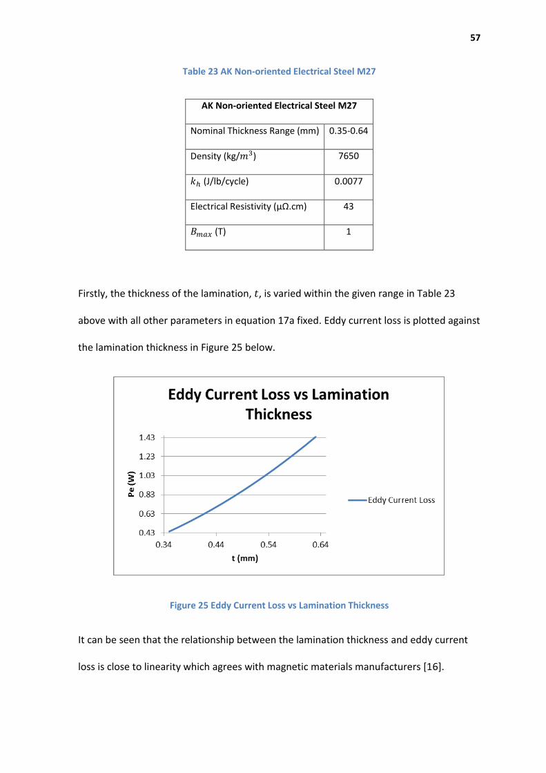
57

Table 23 AK Non-oriented Electrical Steel M27

AK Non-oriented Electrical Steel M27

Nominal Thickness Range (mm) 0.35-0.64

Density (kg/𝑚3) 7650

𝑘ℎ (J/lb/cycle) 0.0077

Electrical Resistivity (µΩ.cm) 43

𝐵𝑚𝑎𝑥 (T) 1

Firstly, the thickness of the lamination, 𝑡, is varied within the given range in Table 23

above with all other parameters in equation 17a fixed. Eddy current loss is plotted against

the lamination thickness in Figure 25 below.

Figure 25 Eddy Current Loss vs Lamination Thickness

It can be seen that the relationship between the lamination thickness and eddy current

loss is close to linearity which agrees with magnetic materials manufacturers [16].

58

However, the relationship is still quadratic as shown in equation 17a. Consequently, eddy

current loss can be minimized by using thin core laminations.

According to the AK Steel datasheet [15], non-oriented steel is available in different

grades (M15, M36, M43, M45 and M47) with different electrical resistivity (see

appendix). Therefore, eddy current loss is calculated at different values of 𝜌. A plot of the

eddy current loss against 𝜌 is shown in Figure 26 below.

Figure 26 Eddy Current loss Against Electrical Resistivity

By varying the electrical resistivity from 37 to 51 µΩ.cm, the eddy current loss drops by

27.53 per cent. This is expected because 𝜌 is inversely proportional to the eddy current

loss as shown in equation 17a.

The maximum flux density in the core, 𝐵𝑚𝑎𝑥, also depends on the core material. The

magnetization curves (B-H curves) for different magnetic materials are shown in Figure 27

below.

0.65

0.7

0.75

0.8

0.85

0.9

0.95

36 41 46 51

Pe

(W)

𝜌(µΩ.cm)

Eddy Current Loss vs Electrical Resistivity

Eddy Current Loss

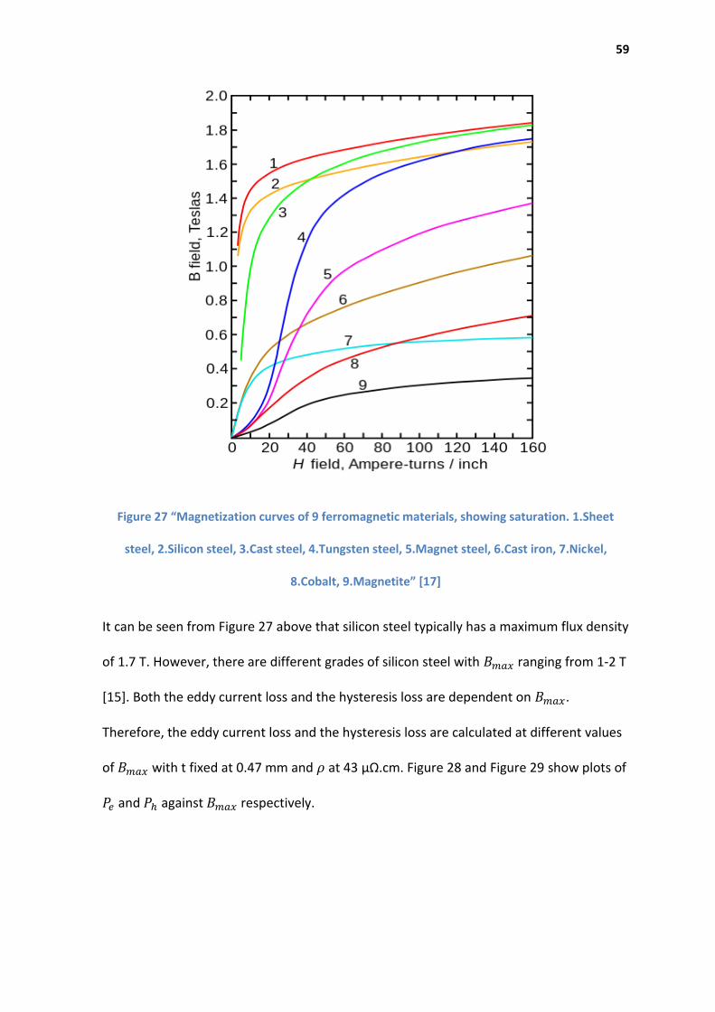
59

Figure 27 “Magnetization curves of 9 ferromagnetic materials, showing saturation. 1.Sheet

steel, 2.Silicon steel, 3.Cast steel, 4.Tungsten steel, 5.Magnet steel, 6.Cast iron, 7.Nickel,

8.Cobalt, 9.Magnetite” [17]

It can be seen from Figure 27 above that silicon steel typically has a maximum flux density

of 1.7 T. However, there are different grades of silicon steel with 𝐵𝑚𝑎𝑥 ranging from 1-2 T

[15]. Both the eddy current loss and the hysteresis loss are dependent on 𝐵𝑚𝑎𝑥.

Therefore, the eddy current loss and the hysteresis loss are calculated at different values

of 𝐵𝑚𝑎𝑥 with t fixed at 0.47 mm and 𝜌 at 43 µΩ.cm. Figure 28 and Figure 29 show plots of

𝑃𝑒 and 𝑃ℎ against 𝐵𝑚𝑎𝑥 respectively.

60

Figure 28 Eddy Current Loss vs. 𝐁𝐦𝐚𝐱

Figure 29 Hysteresis Loss vs. 𝐁𝐦𝐚𝐱

It can be seen that the core losses are highly sensitive to variations in 𝐵𝑚𝑎𝑥. Therefore,

𝐵𝑚𝑎𝑥 is a key design parameter that controls the core losses, which in turn affects the

transformer’s efficiency. Moreover, hysteresis loss is more sensitive to variations in 𝐵𝑚𝑎𝑥

than eddy current loss as shown in Figure 30.

61

Figure 30 Core Losses vs 𝐁𝐦𝐚𝐱

Now, the power losses are related to the efficiency by equation 18 below.

𝜂 =

𝑃𝑜

𝑃𝑜 + 𝑃𝑒 + 𝑃ℎ + 𝑃𝑐

(18)

Substituting the equations of each of the losses gives equation 19 below which directly

relates the design parameters to the efficiency.

𝜂 =

𝐼𝐿𝑉𝐿 cos 𝜃

𝐼𝐿𝑉𝐿 cos 𝜃 +𝜋2𝑓2𝑡2𝐵𝑚𝑎𝑥

2

6𝜌 + 𝑘ℎ𝑓𝐵𝑚𝑎𝑥𝑛 + 𝐼𝐿

2𝑅𝑒𝑞

(19)

The partial derivative of the efficiency with respect to each of the design and electrical

parameters in equation 19 above is given in equation 20 below.

0

1

2

3

4

5

6

7

8

1 1.5 2

Co

re L

oss

es

(W)

𝐵𝑚𝑎𝑥 (T)

Core Losses vs 𝐵𝑚𝑎𝑥

Hysteresis Loss

Eddy Current

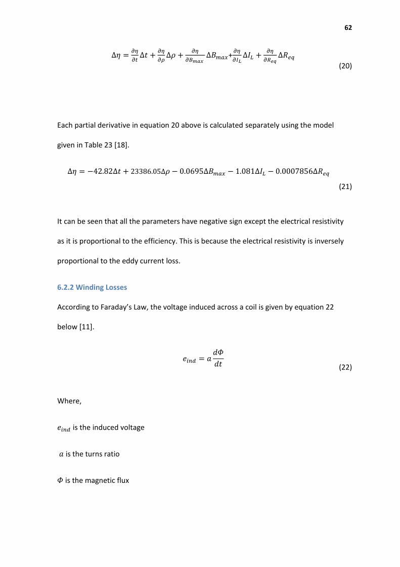
62

∆𝜂 =𝜕𝜂

𝜕𝑡∆𝑡 +

𝜕𝜂

𝜕𝜌∆𝜌 +

𝜕𝜂

𝜕𝐵𝑚𝑎𝑥 ∆𝐵𝑚𝑎𝑥+

𝜕𝜂

𝜕𝐼𝐿∆𝐼𝐿 +

𝜕𝜂

𝜕𝑅𝑒𝑞∆𝑅𝑒𝑞

(20)

Each partial derivative in equation 20 above is calculated separately using the model

given in Table 23 [18].

∆𝜂 = −42.82∆𝑡 + 23386.05∆𝜌 − 0.0695∆𝐵𝑚𝑎𝑥 − 1.081∆𝐼𝐿 − 0.0007856∆𝑅𝑒𝑞

(21)

It can be seen that all the parameters have negative sign except the electrical resistivity

as it is proportional to the efficiency. This is because the electrical resistivity is inversely

proportional to the eddy current loss.

6.2.2 Winding Losses

According to Faraday’s Law, the voltage induced across a coil is given by equation 22

below [11].

𝑒𝑖𝑛𝑑 = 𝑎

𝑑𝛷

𝑑𝑡

(22)

Where,

𝑒𝑖𝑛𝑑 is the induced voltage

𝑎 is the turns ratio

𝛷 is the magnetic flux

63

The equation states that the induced voltage is the rate of change of the flux linkage in

the coil over time per turn. The average flux is proportional to the applied excitation

voltage. Not all the flux in the primary coil passes to the secondary coil due to leakage

flux through air [2]. Therefore, the total average primary flux is composed of a mutual

flux and a leakage flux. The mutual flux stays in the core and reaches the secondary coil.

Equation 23 below shows that the total average primary flux, 𝛷𝑖𝑛, is the sum of the

mutual flux and the leakage flux on the primary side [2].

𝛷𝑖𝑛 = 𝛷𝑀 + 𝛷𝐿𝑃 (23)

Where,

𝛷𝑀 is the mutual flux

𝛷𝐿𝑃 is the primary leakage flux

Now, using equations 22 and 23 above the voltage applied across the primary winding is

re-expressed in terms of the mutual flux and the leakage flux.

𝑣𝑃(𝑡) = 𝑁𝑃

𝑑𝛷𝑀

𝑑𝑡+ 𝑁𝑃

𝑑𝛷𝐿𝑃

𝑑𝑡

(24)

Where,

𝑁𝑃 is the primary winding turns

The same equation (24) applies to the secondary winding, but the number of turns may

be different.

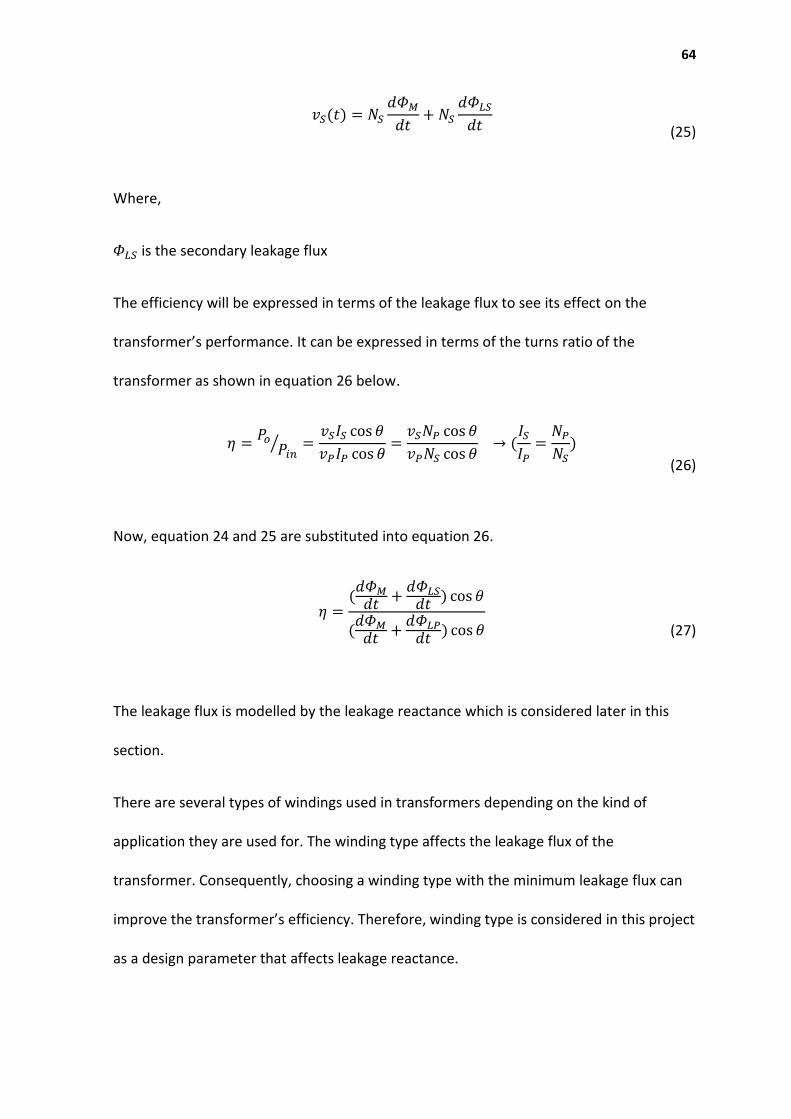
64

𝑣𝑆(𝑡) = 𝑁𝑆

𝑑𝛷𝑀

𝑑𝑡+ 𝑁𝑆

𝑑𝛷𝐿𝑆

𝑑𝑡

(25)

Where,

𝛷𝐿𝑆 is the secondary leakage flux

The efficiency will be expressed in terms of the leakage flux to see its effect on the

transformer’s performance. It can be expressed in terms of the turns ratio of the

transformer as shown in equation 26 below.

𝜂 =

𝑃𝑜𝑃𝑖𝑛

⁄ =𝑣𝑆𝐼𝑆 cos 𝜃

𝑣𝑃𝐼𝑃 cos 𝜃=

𝑣𝑆𝑁𝑃 cos 𝜃

𝑣𝑃𝑁𝑆 cos 𝜃 → (

𝐼𝑆

𝐼𝑃=

𝑁𝑃

𝑁𝑆)

(26)

Now, equation 24 and 25 are substituted into equation 26.

𝜂 =(𝑑𝛷𝑀

𝑑𝑡+

𝑑𝛷𝐿𝑆

𝑑𝑡) cos 𝜃

(𝑑𝛷𝑀

𝑑𝑡+

𝑑𝛷𝐿𝑃

𝑑𝑡) cos 𝜃

(27)

The leakage flux is modelled by the leakage reactance which is considered later in this

section.

There are several types of windings used in transformers depending on the kind of

application they are used for. The winding type affects the leakage flux of the

transformer. Consequently, choosing a winding type with the minimum leakage flux can

improve the transformer’s efficiency. Therefore, winding type is considered in this project

as a design parameter that affects leakage reactance.

65

There are coil arrangements called sandwiches windings, foil windings, distributed helical

or distributed continuous winding. The sandwiches windings main advantages are low

leakage flux and better robustness in large electromagnetic force.

A leakage reactance analysis is carried out by (Kashtiban, Vahedi and Halvaei) on single-

phase, shell-type transformer [19]. The analysis takes the following assumptions into

account:

* The ampere-turns of primary and secondary windings are equal and opposite during

short circuit.

* Saturation is neglected and eddy currents within the conductor and tanks are

neglected.

* Air permeability = 1 and constant.

* All analysis is based on magneto-static.

The design parameters of the transformer used in the analysis are given in Table 24

below.

66

Table 24 Design Parameters of Transformer Used for Winding Type Analysis

Ratings Capacity 150kVA

Voltage 6600/440V

Current 27.73/340.9A

Frequency 50Hz

Phase Single-Phase

Core Type Shell-Type

Material M5

Flux Density 1.7 T

Winding Helical Sandwiches

Current Density (Primary) 1.25 A/mm2

Number of Turns 70 turns

Number of divisions/winding 4 division

The analysis aims to investigate on the effect of winding type on the leakage flux of the

single-phase transformer. Both analytical and simulated models (using FEM) are used to

test the transformer’s performance using helical and sandwiches winding type.

The leakage inductance for a given mean low voltage and high voltage winding turn

length 𝐿𝑚𝑙𝑡 ,an axial winding length 𝑙, radial primary and secondary windings width 𝑐 and

𝑏 respectively and a radial spacing between LV and HV windings 𝑑 is shown in equations

28 and 29 below [19].

1) Helical winding

67

𝐿𝑙𝑒𝑎𝑘𝑎𝑔𝑒 =

𝜇0 𝐿𝑚𝑙𝑡𝑁𝑝2

2𝑊𝑛(𝑑 +

𝑐 + 𝑏

6)

(28)

2) Sandwiches winding

𝐿𝑙𝑒𝑎𝑘𝑎𝑔𝑒 =

𝜇0 𝐿𝑚𝑙𝑡𝑁𝑝2

𝑙(𝑑 +

𝑐 + 𝑏

3)

(29)

Where,

𝐿𝑚𝑙𝑡 Mean length of LV and HV turns

𝑙 Axial length of LV and HV winding (assumed to be the same)

𝑐 Radial width of primary winding

𝑏 Radial width of secondary winding

𝑑 Duct width between LV and HV winding

𝑛 Number of each winding divisions

𝑁𝑝 Number of primary winding turns

It can be seen from the equations above that reducing 𝑑 or 𝑐 results in low leakage

reactance. The equations also indicate that the sandwiches winding always have lower

leakage inductance for the same parameters.

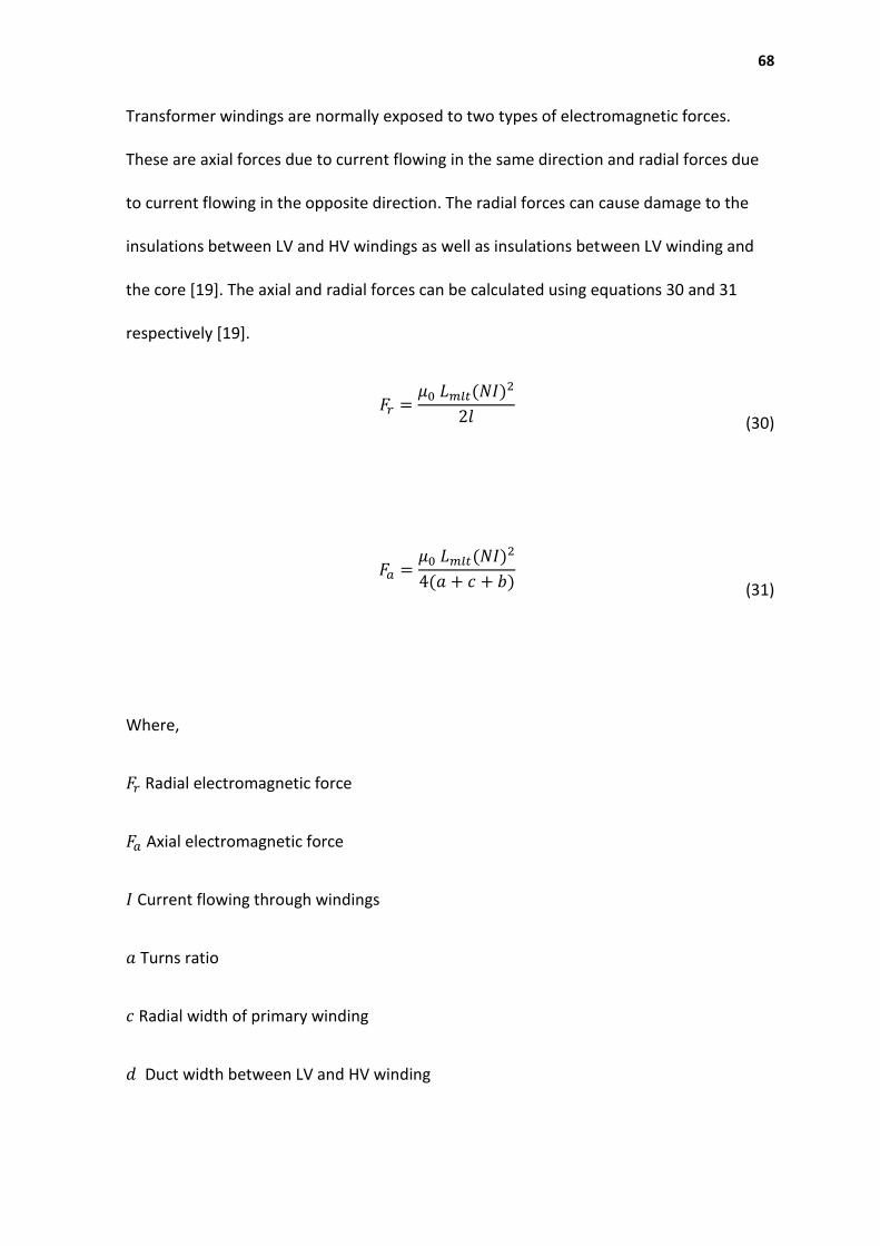
68

Transformer windings are normally exposed to two types of electromagnetic forces.

These are axial forces due to current flowing in the same direction and radial forces due

to current flowing in the opposite direction. The radial forces can cause damage to the

insulations between LV and HV windings as well as insulations between LV winding and

the core [19]. The axial and radial forces can be calculated using equations 30 and 31

respectively [19].

𝐹𝑟 =

𝜇0 𝐿𝑚𝑙𝑡(𝑁𝐼)2

2𝑙

(30)

𝐹𝑎 =

𝜇0 𝐿𝑚𝑙𝑡(𝑁𝐼)2

4(𝑎 + 𝑐 + 𝑏)

(31)

Where,

𝐹𝑟 Radial electromagnetic force

𝐹𝑎 Axial electromagnetic force

𝐼 Current flowing through windings

𝑎 Turns ratio



69

𝐿𝑚𝑙𝑡 Mean length of LV and HV turns

𝜇0 Material permeability

𝑁 Number of winding turns

The total electromagnetic forces in the sandwiches-configured windings are smaller than

the helical-configured windings. This is because of the large radial force in the helical

windings.

The simulation (using FEM) and analytical results both show that the sandwiches

windings give lower leakage inductance and electromagnetic forces. A summary of the

results is shown in Table 25 below.

Table 25 Winding Type Analysis Results

Winding Type Sandwiches Helical

Analytical Simulation Analytical Simulation

Electromagnetic Force (N) 2990 2600 3900 3400

Leakage Inductance (mH) 3.8 4.83 4.2 6.42

As mentioned earlier, part of the flux produced by one coil is not linked to the other. This

leakage flux is modelled by the leakage reactance which is a function of the geometry and

construction of the transformer [20]. Figure 31 shows the top view of a single-phase core-

type transformer with the coils wound on top of each other around the core limb in a

cylindrical form.

70

Figure 31 Windings arrangment of single-phase transformer [3]

Where,


𝑏 Radial width of secondary winding


𝑐 Mean length of turn of the primary winding

Mean length of turn of the secondary winding

Mean length of turn of a hypothetical winding occupying the space between inner and

outer winding

71

The leakage reactance in per cent can be then calculated using equation 32 below [3].

𝑋𝐿(%) =

𝐹(3𝑑 + 𝑏 + 𝑐𝑐)

𝛷𝑚𝑎𝑥𝑙 (32)

Where,

F Ampere-turns of primary or secondary winding

𝛷𝑚𝑎𝑥 Maximum total flux in the core

The maximum total flux of a particular transformer, 𝛷𝑚𝑎𝑥, is the product of the core

cross-sectional area and the maximum flux density. Flux density is determined by

frequency and the number of the winding turns [3]. Therefore, the frequency of the

system to which the transformer is connected is controlled within close limits in order to

avoid variations in the nominal voltage. Consequently the flux density is maintained at a

value close to saturation.

Therefore, a combination of 𝛷𝑚𝑎𝑥 and 𝑙 can be selected to provide the desired value of

the leakage reactance. The winding also have resistance, but it is relatively small

compared to the reactance so that the winding impedance can be approximated by the

winding reactance [3].

Note: In practice, there are several methods to determine the leakage reactance of a

transformer such as the FEM simulator [21].

72

7.0 Conclusions and Future Work

The complete equivalent circuit of the LabVolt power transformer was developed by

carrying out laboratory-based experiments. The optimal loading on the transformer at

the rated voltage with the maximum efficiency occurs at 60 per cent of the rated load

current which corresponds to a load impedance of 1600 Ω. The maximum efficiency was

88.89 per cent with a purely resistive load. However, the lowest voltage regulation (-3.14

per cent) occurred in the purely capacitive load case.

A computer based simulation model was built in ICAPS to verify the experimental results.

The simulated model was also used to carry out a sensitivity analysis on the model

parameters. The sensitivity analysis shows how variations in the model parameters affect

fixed and variable losses. ICAPS generally gave results that are reasonably close to the

experimental results. Both the experimental and the simulation results were also verified

by the literature reviewed in this project. However, ICAPS has limitations such as not

including practical factors that can affect losses in the transformer.

A general conclusion can be drawn from the voltage regulation experiments and

simulations is that the higher the load current the higher the voltage drop across the

winding resistance which results in a poorer voltage regulation. Furthermore, different

load types (resistive, inductive and capacitive) have different regulation curves and the

resistive load has the poorest voltage regulation.

This project mainly analysed and discussed the performance of a single-phase power

transformer under various loading. The key involvement of the project was to carry out

experimental procedures (open-circuit test and short-circuit test) to find the model

parameters of the transformer’s complete equivalent circuit. The complete equivalent

73

circuit models various losses in the transformer. The transformer’s efficiency and voltage

regulation were analysed both experimentally and on the simulations. ICAPS was very

helpful in analysing the effect of variations in each model parameter on the power loss

associated with it. Experimental tests are to be carried out for more accurate estimation

of the power loss.

74

8.0 Annotated Bibliography

-S. J. Chapman, Electric Machinery Fundamentals, 4th Edition. New York: The McGraw-

Hill Companies, 2005, pp. 65-108.

In this book, Chapman did an extensive study on power transformers in chapter2. He

covered transformers construction, operation, parameters, voltage regulation, efficiency,

connections and ratings. The relevance of the book to this project arises in transformers

core construction and losses. Equivalent circuits were used to determine the model

parameters (open-circuit and short-circuit test). Finally, voltage regulation and efficiency

equations are also used.

-B. S. Guru and H. R. Hiziroglu, Electric Machinery And Transformers, 3rd Edition. New

York: Oxford University Press, 2001, pp. 202-239

Chapter 4 of this book also explores transformers construction, non-ideal transformer

(practical), maximum efficiency criterion, determination of parameters, and per-unit

computations and current transformers. In this project, the characteristics of a practical

transformer were understood. The maximum efficiency criterion section is also useful for

efficiency optimization.

-M. J. Heathcote, J&P Transformer Book, 13th Edition. Britain: Newnes, 2007, pp. 14-

36,105-285.

This book covers all aspects about transformers including losses, design parameters,

construction materials and configurations, operation and applications. The second part of

this project will be about transformer design parameters. Chapter 2 of this book is useful

for the transformer design aspect.

75

-Amoiralis, Eleftherios I. “Transformer Design and Optimization; A Literature Survey,”

IEEE transactions on power delivery, vol. 24, no.4, pp. 1990-2024 Oct. 2009.

This journal article conducts a literature survey on transformer design and optimization

research over the past 35 years based on previously published resources. This paper is

used to support the literature review of this project in the design parameters aspect.

-Georgilakis, P.S. & Amoiralis, E.I. , "Spotlight on transformer design", IEEE Power and

Energy Magazine, vol. 5, no. 1, pp. 40-50, Feb. 2007

This paper considers winding material selection in order to find an optimum transformer

design. Therefore, it covers one of the significant design parameters in this project. The

effect of the winding material variations on the transformer performance is discussed.

-Subramanian, S. & Padma, S. , "Optimal Design of Single Phase Transformer Using

Bacterial Foraging Algorithm", International Journal of Engineering Science and

Technology, vol. 3, no. 4, pp. 2677-2684, Apr. 2011.

This paper finds the optimum design of a single phase transformer to minimize the cost

and improve the efficiency. Even though cost is not considered in this project, the paper

considers ways to optimize the efficiency.

76

9.0 References

[1] B. S. Guru and H. R. Hiziroglu, Electric Machinery And Transformers, 3rd Edition. New York:

Oxford University Press, 2001, pp. 202-239

[2] S. J. Chapman, Electric Machinery Fundamentals, 4th Edition. New York: The McGraw-Hill

Companies, 2005, pp. 65-108.

[3] M. J. Heathcote, J&P Transformer Book: A Practical Technology of The Power Transformer, 13th

ed. GB: Newnes, 2007, pp. 105-285.

[4] G. Crebbin and S. Hettiwatte, “Measurement of Transformer Model Parameters,

Performance and Ratings,” Murdoch University, Murdoch, WA, March 2015. Electromechanical

Energy Conversion (ENG347) Lecture Notes.

[http://handbook.murdoch.edu.au/units/details/?unit=ENG347&year=2015]. [Accessed: Sep. 4,

2015].

[5] E. Cardelli, A. Faba and F. Tissi “Prediction and Control of Transformer Inrush Currents”, “IEEE

Transactions on Magnetics”, vol. 51, no. 3, pp. 1-4, March 2015.

[6]“LabVolt Single-Phase Transformer 8341-0A Datasheet”, LabVolt Series,Nov

2015.[Online].Available: https://www.labvolt.com. [Accessed Nov 9 2015].

[7] “PM 100/300 Power Analyzer User Manual” Voltech Instruments, Aug 9

2010.[Online].Available: http://www.voltech.com/Support/Downloads.aspx. [Accessed: Aug 26

2015].

http://www.voltech.com/Support/Downloads.aspx

77

[8] S. Hettiwatte, “Transformer Regulation Experiment 3”, Murdoch University, Murdoch, WA,

March 2015. Electromechanical Energy Conversion (ENG347) Laboratory Book.

[http://handbook.murdoch.edu.au/units/details/?unit=ENG347&year=2015]. [Accessed: Aug. 3,

2015].

[9] K. Rajagopal,Engineering Physics, Part 2.New Delhi: PHI Learning Private LTD, 2009, pp. 71

[10] R. K. Rajput, A Text Book of Electrical Engineering, 2nd Ed. New Delhi: Laxmi Publications (P)

LTD,2004,pp. (262-269).

[11] S.V. Kulkarni and S.A. Khaparde, Transformer Engineering: Design,Technology and

Diagnostics,2nd Ed. United States of America: Taylor & Francis Group CRC Press, 2012,pp.45

[12] Hambley, A.R. 2011, Electrical engineering: principles and applications, 5th, International

edn, Pearson Education, Upper Saddle River, N.J.

[13] Pry RH, Bean CP (1958) Calculation of the energy loss in magnetic sheet materials using a

domain model. J Appl Phys 29:532–533.

[14] J. C. Olivares-Galvan, P. S. Georgilakis, E. Campero-Littlewood and R. Escarela-Perez. “Core

lamination selection for distribution transformers based on sensitivity analysis”, “Electrical

Engineering”, vol. 95, no. 1, pp. 33-42, March 2013.

[15] “Nonoriented Elecrtical Steels”, AK Steels,2007.[Online].Available:

www.aksteel.com/pdf/markets_products/.../non_oriented_bulletin.pdf. [Acessed: Oct 26 2015].

http://www.aksteel.com/pdf/markets_products/.../non_oriented_bulletin.pdf

78

[16] “Grain-Oriented Electrical Steel”, ATI Steels,2012.[Online]. Available:

https://www.atimetals.com/products/Pages/grain-oriented-electrical-steel-goes.aspx. [Accessed:

Oct 24 2015].

[17]Steinmetz, Charles (1917). "fig. 42". Theory and Calculation of Electric Circuits. McGraw-Hill.

[18] V. Weiss, “Partial Differentiation Using the Quotient Role”, Swinburne Commons, Swinburne

University, Jun 14 2012.[Online]. Available: https://www.youtube.com/watch?v=z14ur1xlq9k.

[Accessed: Nov 9 2015].

[19] A.M. Kashtiban, , A. Vahedi, & A. Halvaei, “Investigation of winding type effect on leakage

flux of single phase shell type transformer using FEM” in Electrical Machines and Systems, 2005.

ICEMS 2005. Proceedings of the Eighth International Conference on (Volume:3 ), Sept. 29, 2005,

Nanjing.Tehran: IEEE, 2005. pp. 1755-1758.

[20] A.N. Jahromi, J. Faiz and H. Mohseni “A Fast Method for Calculation of Transformers Leakage

Reactance Using Energy Technique”, “IJE Transactions B: Applications” vol. 16, no. 1, pp. 41-48,

April 2003.

[21] G. Alonso and J. Antonio, “A New Method for Calculating of Leakage Reactances and Iron

Losses in Transformers”, 5th International Conference on Electrical Machines and Systems,

(ICEMS 2001), Vol. 1, 178-181.

https://www.atimetals.com/products/Pages/grain-oriented-electrical-steel-goes.aspx

https://www.youtube.com/watch?v=z14ur1xlq9k

http://murdoch.summon.serialssolutions.com/2.0.0/link/0/eLvHCXMwhV3dS8MwED-GT4rg18Spgz746pY2tW1g7GVsuIeBoPhakjZBsXRjH-if55_mJW2yKsM9FC6XkKSh3F0vd78DoEGP3P-RCcKXKmIPjKk8EzxKmIxYJGOBDw-Jii06gwlTbYGtsqjrnZhQNNnTpLnZx_aqz8Uq5UVhYAX5si6e4aPpgeYHymMaEP2FR9Otv4VQhpYBwx8zHKQLzqBurAB4XDusbz19wvrT0Xj2XLlcAlTBGsGyUX3FKJ_JCbw6Z9iOnWoRuBPte-8bnEJ7m-_nPTlNdgYtWZ7DUQOq8AK-B2LYwOSYl4O-GHrInCvv892kxliO9upaugoXcWNLr5D8A0WY5ahi89WYSTsuCte5eEMVaxsrHbG6a4m1Nb3l0rJ0ML_bzmQ802Qb7ibjl9GjOcN0UYFspMSYr1GYkDCnmZ_RSzjmOui_XJvkwPwKPIH2iZKU5QnLQpnFCctFzAOVMV_RkPMOdH7PWZ9vushVB7r_rne9p_8GDg2Kq_HG3MLBermRXVeE6gde4-JE

http://murdoch.summon.serialssolutions.com/2.0.0/link/0/eLvHCXMwhV3dS8MwED-GT4rg18Spgz746pY2tW1g7GVsuIeBoPhakjZBsXRjH-if55_mJW2yKsM9FC6XkKSh3F0vd78DoEGP3P-RCcKXKmIPjKk8EzxKmIxYJGOBDw-Jii06gwlTbYGtsqjrnZhQNNnTpLnZx_aqz8Uq5UVhYAX5si6e4aPpgeYHymMaEP2FR9Otv4VQhpYBwx8zHKQLzqBurAB4XDusbz19wvrT0Xj2XLlcAlTBGsGyUX3FKJ_JCbw6Z9iOnWoRuBPte-8bnEJ7m-_nPTlNdgYtWZ7DUQOq8AK-B2LYwOSYl4O-GHrInCvv892kxliO9upaugoXcWNLr5D8A0WY5ahi89WYSTsuCte5eEMVaxsrHbG6a4m1Nb3l0rJ0ML_bzmQ802Qb7ibjl9GjOcN0UYFspMSYr1GYkDCnmZ_RSzjmOui_XJvkwPwKPIH2iZKU5QnLQpnFCctFzAOVMV_RkPMOdH7PWZ9vushVB7r_rne9p_8GDg2Kq_HG3MLBermRXVeE6gde4-JE

http://ieeexplore.ieee.org/xpl/mostRecentIssue.jsp?punumber=10523

http://ieeexplore.ieee.org/xpl/mostRecentIssue.jsp?punumber=10523

79

10.0 Appendix Equation 14 is derived by . Guru and Hiziroglu [1]. The output power is given in terms of the load

current by referring the load to the primary side (this is where 𝑎 comes from). The load current at

maximum efficiency is then derived as shown below.

Recalling equation 14

𝜂 =𝑎𝑉𝐿𝐼𝐿𝑃𝐹

𝑎𝑉𝐿𝐼𝐿𝑃𝐹 + 𝑃𝑚 + 𝐼𝐿2𝑅𝑒𝑞

× 100%

Equation 14 is differentiated with respect to 𝐼𝐿 and setting it equal to zero.

𝐼𝐿𝜂2 𝑅𝑒𝑞 = 𝑃𝑚

The load current at maximum efficiency (given in equation 15) then becomes

𝐼𝐿𝜂 = √𝑃𝑚

𝑅𝑒𝑞

Table 26 indicates the core losses for various materials with different thicknesses at 60 Hz [##].

Table 26 Core Losses for Different Materials

Material Thickness (mm) 𝑷𝒉 (W/kg) 𝑷𝒆 (W/kg)

Grain-oriented 3% SiFe 0.29 0.34 0.29

Grain-oriented 3% SiFe 0.34 1.7 0.31

Nonoriented 3% SiFe 0.35 1.8 0.29

Amorphous 0.3 0.29 0.00085

Table 27 shows the electrical resistivity for different AK non-oriented electrical steel grades [AK].

Table 27 AK Non-oriented Electrical Steel Resistivity

Grade Electrical Resistivity (µΩ.cm)

M15 50

M27 43

M36 43

M43 43

M45 37

M47 37

Table 28 shows the data used to plot eddy current loss against the lamination thickness in Figure

25.

80

Table 28 Eddy Current Loss vs Lamination Thickness

𝒕(mm) 𝑷𝒆 (W)

0.35 0.444

0.37 0.496

0.39 0.551

0.41 0.609

0.43 0.669

0.45 0.733

0.47 0.799

0.49 0.869

0.51 0.942

0.53 1.017

0.55 1.095

0.57 1.176

0.59 1.26

0.61 1.35

0.63 1.44

Table 29 shows the data used to plot eddy current loss against the electrical resistivity in Figure

26.

Table 29 Eddy Current Loss vs Electrical Resistivity

𝝆 (µΩ.cm) 𝑷𝒆 (W)

51 0.674

50 0.688

49 0.702

48 0.717

47 0.732

46 0.748

45 0.764

44 0.782

43 0.8

42 0.819

41 0.839

40 0.86

39 0.882

38 0.905

37 0.93

Table 30 shows the data used to plot core losses of silicon steel at different values of 𝐵𝑚𝑎𝑥 in

Figure 28 and Figure 29.

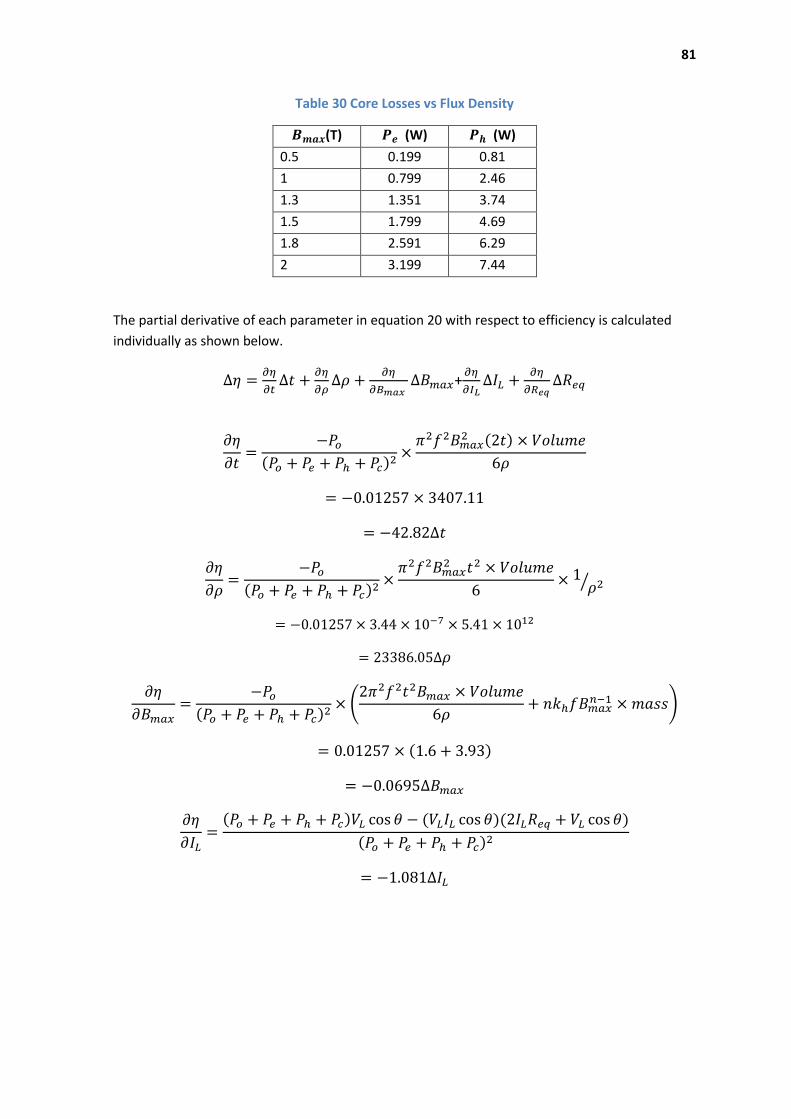
81

Table 30 Core Losses vs Flux Density

𝑩𝒎𝒂𝒙(T) 𝑷𝒆 (W) 𝑷𝒉 (W)

0.5 0.199 0.81

1 0.799 2.46

1.3 1.351 3.74

1.5 1.799 4.69

1.8 2.591 6.29

2 3.199 7.44

The partial derivative of each parameter in equation 20 with respect to efficiency is calculated

individually as shown below.

∆𝜂 =𝜕𝜂

𝜕𝑡∆𝑡 +

𝜕𝜂

𝜕𝜌∆𝜌 +

𝜕𝜂

𝜕𝐵𝑚𝑎𝑥 ∆𝐵𝑚𝑎𝑥+

𝜕𝜂

𝜕𝐼𝐿∆𝐼𝐿 +

𝜕𝜂

𝜕𝑅𝑒𝑞∆𝑅𝑒𝑞

𝜕𝜂

𝜕𝑡=

−𝑃𝑜

(𝑃𝑜 + 𝑃𝑒 + 𝑃ℎ + 𝑃𝑐)2×

𝜋2𝑓2𝐵𝑚𝑎𝑥2 (2𝑡) × 𝑉𝑜𝑙𝑢𝑚𝑒

6𝜌

= −0.01257 × 3407.11

= −42.82∆𝑡

𝜕𝜂

𝜕𝜌=

−𝑃𝑜

(𝑃𝑜 + 𝑃𝑒 + 𝑃ℎ + 𝑃𝑐)2×

𝜋2𝑓2𝐵𝑚𝑎𝑥2 𝑡2 × 𝑉𝑜𝑙𝑢𝑚𝑒

6× 1

𝜌2⁄

= −0.01257 × 3.44 × 10−7 × 5.41 × 1012

= 23386.05∆𝜌

𝜕𝜂

𝜕𝐵𝑚𝑎𝑥=

−𝑃𝑜

(𝑃𝑜 + 𝑃𝑒 + 𝑃ℎ + 𝑃𝑐)2× (

2𝜋2𝑓2𝑡2𝐵𝑚𝑎𝑥 × 𝑉𝑜𝑙𝑢𝑚𝑒

6𝜌+ 𝑛𝑘ℎ𝑓𝐵𝑚𝑎𝑥

𝑛−1 × 𝑚𝑎𝑠𝑠)

= 0.01257 × (1.6 + 3.93)

= −0.0695∆𝐵𝑚𝑎𝑥

𝜕𝜂

𝜕𝐼𝐿=

(𝑃𝑜 + 𝑃𝑒 + 𝑃ℎ + 𝑃𝑐)𝑉𝐿 cos 𝜃 − (𝑉𝐿𝐼𝐿 cos 𝜃)(2𝐼𝐿𝑅𝑒𝑞 + 𝑉𝐿 cos 𝜃)

(𝑃𝑜 + 𝑃𝑒 + 𝑃ℎ + 𝑃𝑐)2

= −1.081∆𝐼𝐿

82

𝜕𝜂

𝜕𝑅𝑒𝑞=

−𝑃𝑜

(𝑃𝑜 + 𝑃𝑒 + 𝑃ℎ + 𝑃𝑐)2× 𝐼𝐿

2

= −0.01257 × 0.252

= −0.0007856∆𝑅𝑒𝑞

Date post:	11-Sep-2019
Category:	Documents
Upload:	others
View:	2 times
Download:	0 times

Power Transformer Modelling for Optimal Performance · transformer’s efficiency and voltage...

Documents