69
PowerPoint to accompany Chapter 7 Firms in Perfectly Competitive Markets
| Date post: | 23-Dec-2015 |
| Category: |
Documents |
| Upload: | joseph-grant |
| View: | 236 times |
| Download: | 2 times |
PowerPoint
to accompany
Chapter 7
Firms in Perfectly
Competitive Markets
Hubbard, Garnett, Lewis and O’Brien: Essentials of Economics © 2010 Pearson Australia
1. Define a perfectly competitive market, and explain why a perfect competitor faces a horizontal demand curve.
2. Explain how a perfect competitor decides how much to produce.
3. Use graphs to show a firm’s profit or loss.
Learning Objectives
Hubbard, Garnett, Lewis and O’Brien: Essentials of Economics © 2010 Pearson Australia
4. Explain why firms may shut down temporarily.
5. Explain how entry and exit ensure that firms earn zero economic profit in the long run.
6. Explain how perfect competition leads to economic efficiency.
Learning Objectives
Hubbard, Garnett, Lewis and O’Brien: Essentials of Economics © 2010 Pearson Australia
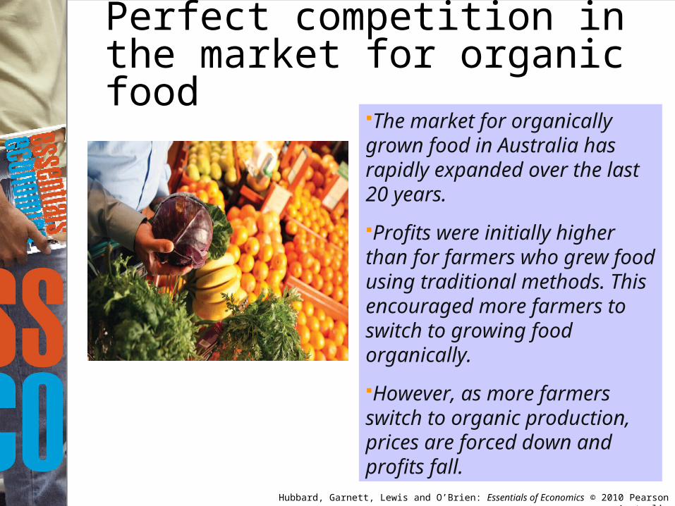
The market for organically grown food in Australia has rapidly expanded over the last 20 years.
Profits were initially higher than for farmers who grew food using traditional methods. This encouraged more farmers to switch to growing food organically.
However, as more farmers switch to organic production, prices are forced down and profits fall.
Perfect competition in the market for organic food
Hubbard, Garnett, Lewis and O’Brien: Essentials of Economics © 2010 Pearson Australia
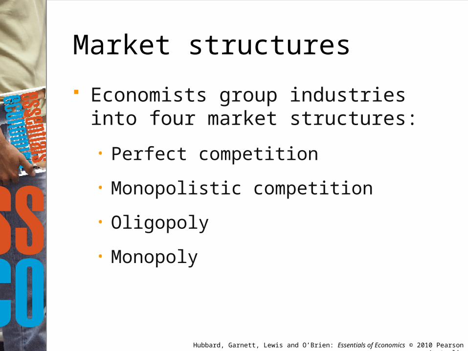
Market structures
Economists group industries into four market structures:
• Perfect competition
• Monopolistic competition
• Oligopoly
• Monopoly
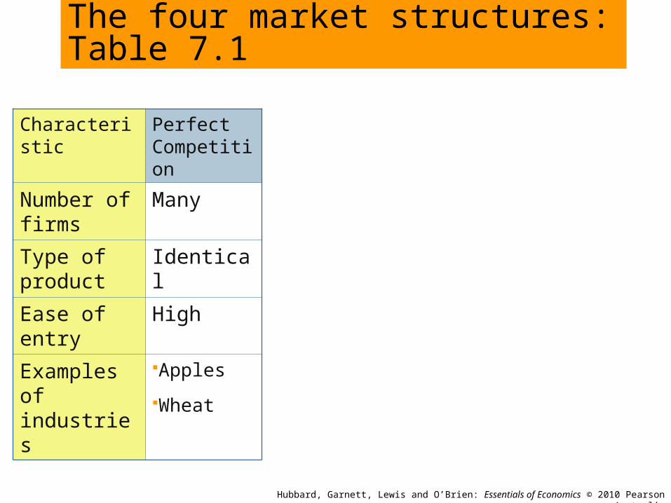
The four market structures: Table 7.1
Characteristic Perfect Competition
Number of firms
Many
Type of product
Identical
Ease of entry
High
Examples of industries
Apples
Wheat
Hubbard, Garnett, Lewis and O’Brien: Essentials of Economics © 2010 Pearson Australia
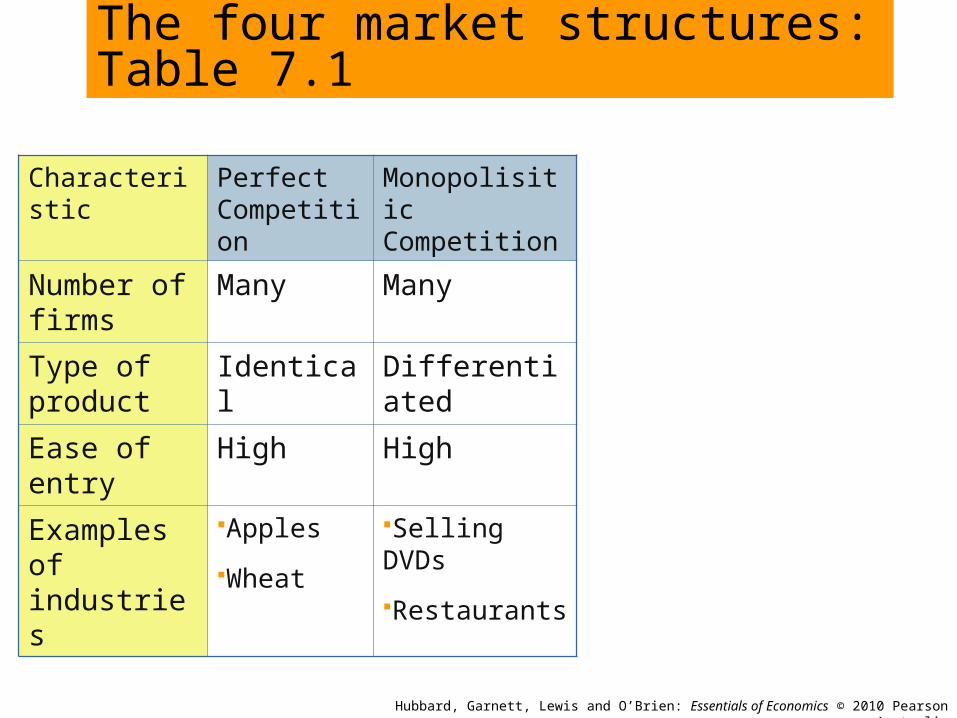
The four market structures: Table 7.1
Characteristic Perfect Competition
Monopolisitic Competition
Number of firms
Many Many
Type of product
Identical Differentiated
Ease of entry
High High
Examples of industries
Apples
Wheat
Selling DVDs
Restaurants
Hubbard, Garnett, Lewis and O’Brien: Essentials of Economics © 2010 Pearson Australia
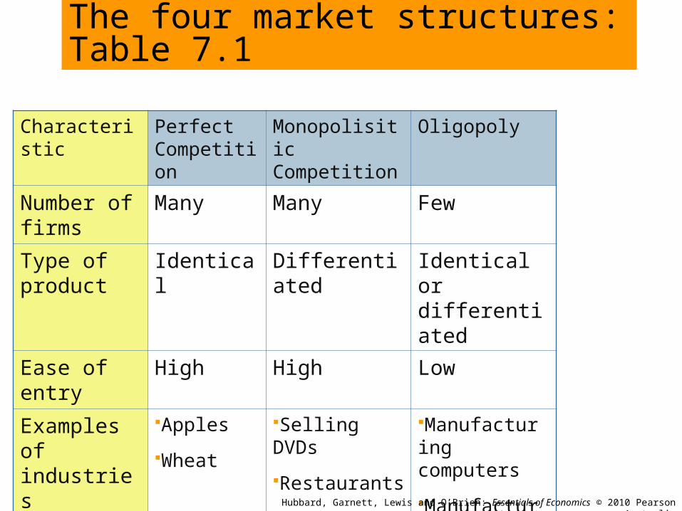
The four market structures: Table 7.1
Characteristic Perfect Competition
Monopolisitic Competition
Oligopoly
Number of firms
Many Many Few
Type of product
Identical Differentiated Identical or differentiated
Ease of entry
High High Low
Examples of industries
Apples
Wheat
Selling DVDs
Restaurants
Manufacturing computers
Manufacturing cars
Hubbard, Garnett, Lewis and O’Brien: Essentials of Economics © 2010 Pearson Australia
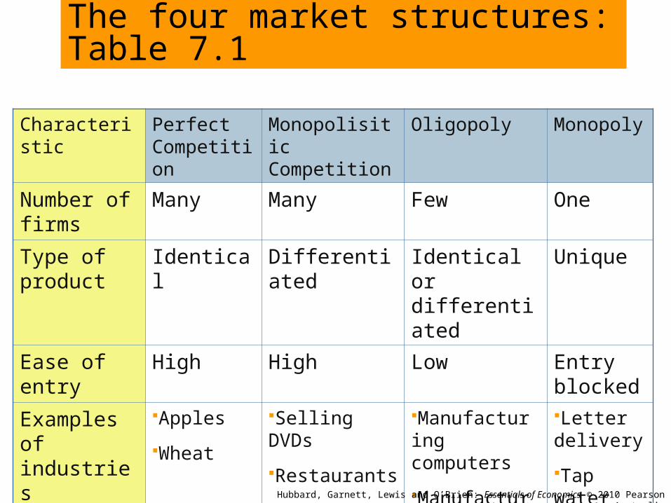
The four market structures: Table 7.1
Characteristic Perfect Competition
Monopolisitic Competition
Oligopoly Monopoly
Number of firms
Many Many Few One
Type of product
Identical Differentiated Identical or differentiated
Unique
Ease of entry
High High Low Entry blocked
Examples of industries
Apples
Wheat
Selling DVDs
Restaurants
Manufacturing computers
Manufacturing cars
Letter delivery
Tap water
Hubbard, Garnett, Lewis and O’Brien: Essentials of Economics © 2010 Pearson Australia
Hubbard, Garnett, Lewis and O’Brien: Essentials of Economics © 2010 Pearson Australia
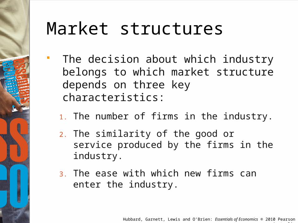
Market structures
The decision about which industry belongs to which market structure depends on three key characteristics:
1. The number of firms in the industry.
2. The similarity of the good or service produced by the firms in the industry.
3. The ease with which new firms can enter the industry.

Hubbard, Garnett, Lewis and O’Brien: Essentials of Economics © 2010 Pearson Australia
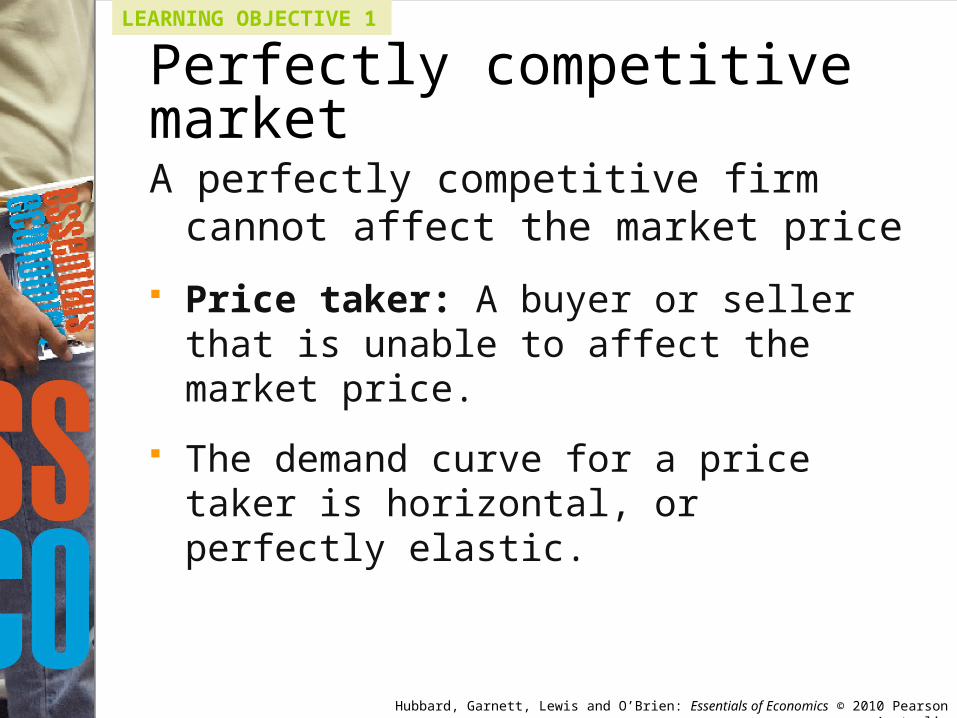
Perfectly competitive market
LEARNING OBJECTIVE 1
Perfectly competitive market: A market that meets the conditions of:
1. Many buyers and sellers, all of whom are small relative to the market.
2. All firms selling identical products.
3. There are no barriers to new firms entering the market.
Hubbard, Garnett, Lewis and O’Brien: Essentials of Economics © 2010 Pearson Australia
Perfectly competitive market
LEARNING OBJECTIVE 1
A perfectly competitive firm cannot affect the market price
Price taker: A buyer or seller that is unable to affect the market price.
The demand curve for a price taker is horizontal, or perfectly elastic.
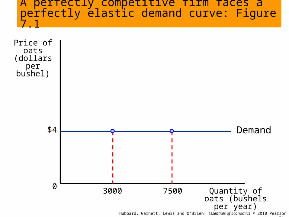
Price of oats (dollars per bushel)
Quantity of oats (bushels per year)
03000
A perfectly competitive firm faces a perfectly elastic demand curve: Figure 7.1
Hubbard, Garnett, Lewis and O’Brien: Essentials of Economics © 2010 Pearson Australia
Demand$4
7500
Hubbard, Garnett, Lewis and O’Brien: Essentials of Economics © 2010 Pearson Australia
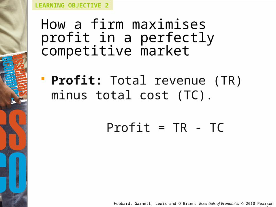
Profit: Total revenue (TR) minus total cost (TC).
Profit = TR - TC
LEARNING OBJECTIVE 2
How a firm maximises profit in a perfectly competitive market
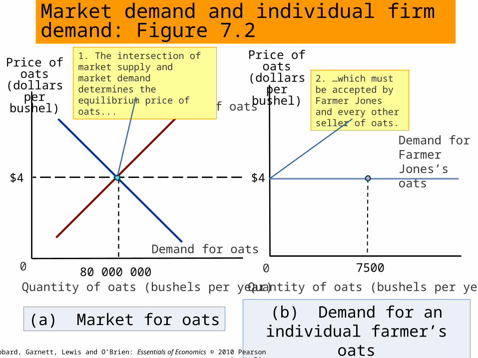
(b) Demand for an individual farmer’s oats
0
(a) Market for oats
Quantity of oats (bushels per year)
Supply of oats
Demand for oats
$4
Demand for Farmer Jones’s oats
Market demand and individual firm demand: Figure 7.2
2. …which must be accepted by Farmer Jones and every other seller of oats.
80 000 000
Price of oats (dollars per
bushel)
Price of oats (dollars per
bushel)
Quantity of oats (bushels per year)
0 7500
$4
1. The intersection of market supply and market demand determines the equilibrium price of oats...
Hubbard, Garnett, Lewis and O’Brien: Essentials of Economics © 2010 Pearson Australia
Hubbard, Garnett, Lewis and O’Brien: Essentials of Economics © 2010 Pearson Australia
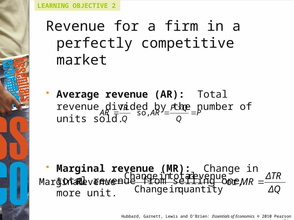
Revenue for a firm in a perfectly competitive market
Average revenue (AR): Total revenue divided by the number of units sold.
Marginal revenue (MR): Change in total revenue from selling one more unit.
Q
TRAR
LEARNING OBJECTIVE 2
PQ
QPAR
so,
or, ΔQ
ΔTRMR
quantity in Change
revenue total in Change Revenue Marginal
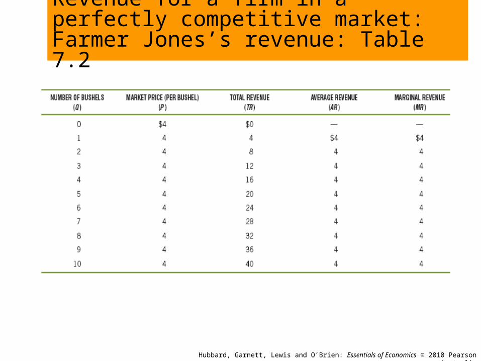
Revenue for a firm in a perfectly competitive market: Farmer Jones’s revenue: Table 7.2
Hubbard, Garnett, Lewis and O’Brien: Essentials of Economics © 2010 Pearson Australia
Hubbard, Garnett, Lewis and O’Brien: Essentials of Economics © 2010 Pearson Australia
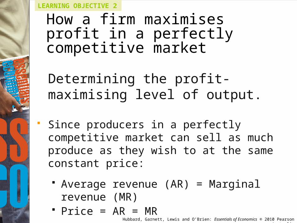
Determining the profit-maximising level of output.
Since producers in a perfectly competitive market can sell as much produce as they wish to at the same constant price:
Average revenue (AR) = Marginal revenue (MR) Price = AR = MR
LEARNING OBJECTIVE 2
How a firm maximises profit in a perfectly competitive market
Hubbard, Garnett, Lewis and O’Brien: Essentials of Economics © 2010 Pearson Australia
How a firm maximises profit in a perfectly competitive market
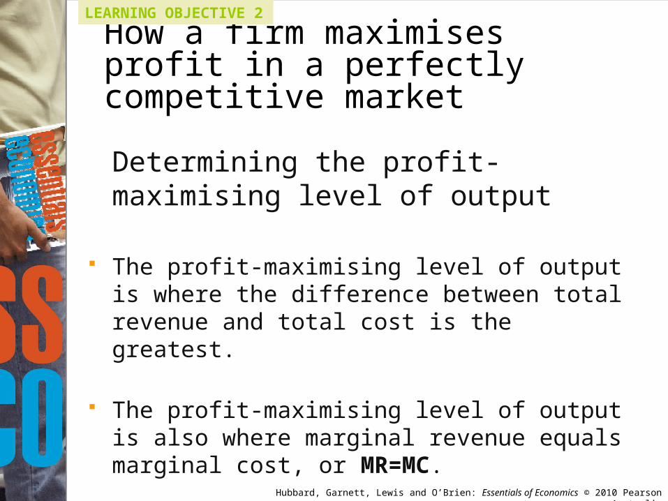
Determining the profit-maximising level of output
The profit-maximising level of output is where the difference between total revenue and total cost is the greatest.
The profit-maximising level of output is also where marginal revenue equals marginal cost, or MR=MC.
LEARNING OBJECTIVE 2
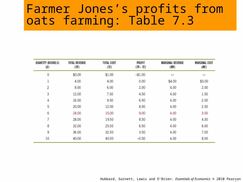
Farmer Jones’s profits from oats farming: Table 7.3
Hubbard, Garnett, Lewis and O’Brien: Essentials of Economics © 2010 Pearson Australia
Hubbard, Garnett, Lewis and O’Brien: Essentials of Economics © 2010 Pearson Australia
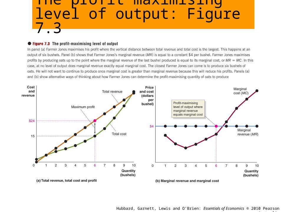
The profit maximising level of output: Figure 7.3
Hubbard, Garnett, Lewis and O’Brien: Essentials of Economics © 2010 Pearson Australia
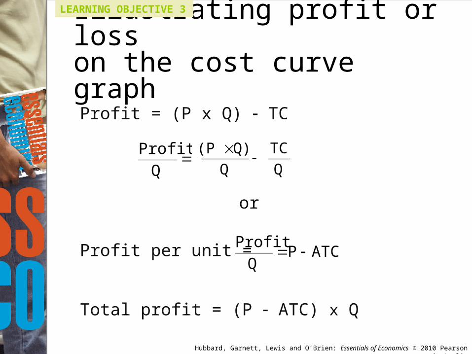
Illustrating profit or losson the cost curve graph
Profit = (P x Q) TC
or
Profit per unit =
Total profit = (P ATC) x Q
LEARNING OBJECTIVE 3
QQ)(P
Q
ProfitQTC
ATCPQ
Profit
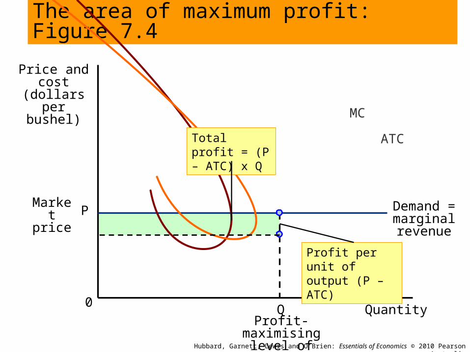
Price and cost (dollars per bushel)
Quantity0
The area of maximum profit: Figure 7.4
Hubbard, Garnett, Lewis and O’Brien: Essentials of Economics © 2010 Pearson Australia
Demand = marginal revenue
P
Q
Market price
Profit-maximising level of output
MC
ATCTotal profit = (P – ATC) x Q
Profit per unit of output (P – ATC)
Hubbard, Garnett, Lewis and O’Brien: Essentials of Economics © 2010 Pearson Australia
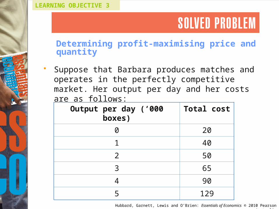
Determining profit-maximising price and quantity
LEARNING OBJECTIVE 3
Suppose that Barbara produces matches and operates in the perfectly competitive market. Her output per day and her costs are as follows:
Output per day (‘000 boxes) Total cost
0 20
1 40
2 50
3 65
4 90
5 129
Hubbard, Garnett, Lewis and O’Brien: Essentials of Economics © 2010 Pearson Australia
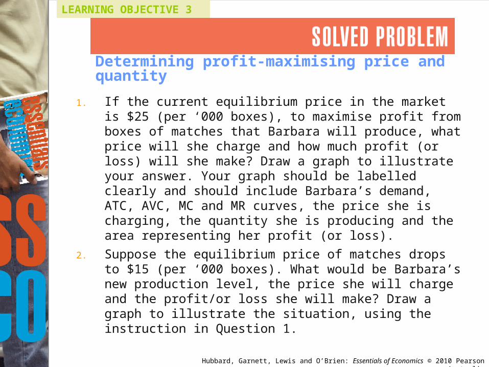
Determining profit-maximising price and quantity
LEARNING OBJECTIVE 3
1. If the current equilibrium price in the market is $25 (per ‘000 boxes), to maximise profit from boxes of matches that Barbara will produce, what price will she charge and how much profit (or loss) will she make? Draw a graph to illustrate your answer. Your graph should be labelled clearly and should include Barbara’s demand, ATC, AVC, MC and MR curves, the price she is charging, the quantity she is producing and the area representing her profit (or loss).
2. Suppose the equilibrium price of matches drops to $15 (per ‘000 boxes). What would be Barbara’s new production level, the price she will charge and the profit/or loss she will make? Draw a graph to illustrate the situation, using the instruction in Question 1.
Hubbard, Garnett, Lewis and O’Brien: Essentials of Economics © 2010 Pearson Australia
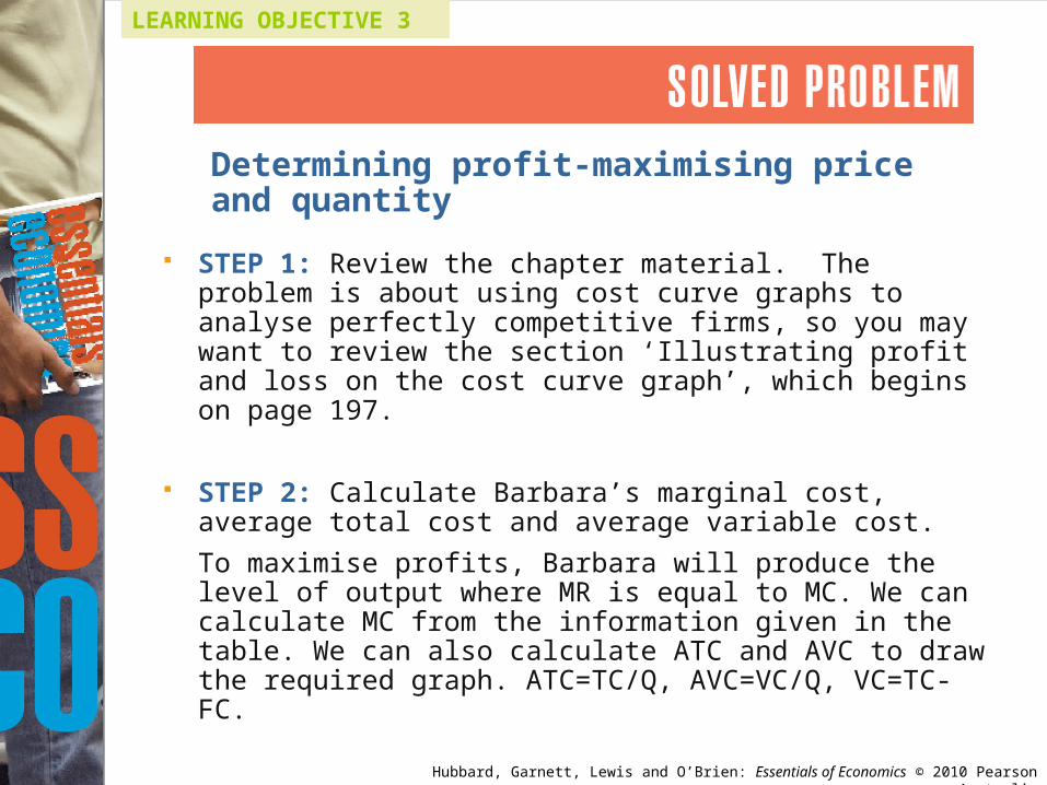
LEARNING OBJECTIVE 3
Determining profit-maximising price and quantity
STEP 1: Review the chapter material. The problem is about using cost curve graphs to analyse perfectly competitive firms, so you may want to review the section ‘Illustrating profit and loss on the cost curve graph’, which begins on page 197.
STEP 2: Calculate Barbara’s marginal cost, average total cost and average variable cost.
To maximise profits, Barbara will produce the level of output where MR is equal to MC. We can calculate MC from the information given in the table. We can also calculate ATC and AVC to draw the required graph. ATC=TC/Q, AVC=VC/Q, VC=TC-FC.
Hubbard, Garnett, Lewis and O’Brien: Essentials of Economics © 2010 Pearson Australia
LEARNING OBJECTIVE 3
Determining profit-maximising price and quantity
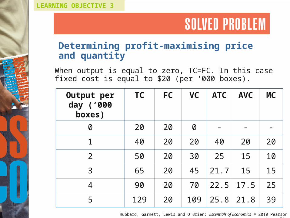
When output is equal to zero, TC=FC. In this case fixed cost is equal to $20 (per ‘000 boxes).
Output per day (‘000 boxes)
TC FC VC ATC AVC MC
0 20 20 0 - - -
1 40 20 20 40 20 20
2 50 20 30 25 15 10
3 65 20 45 21.7 15 15
4 90 20 70 22.5 17.5 25
5 129 20 109 25.8 21.8 39
Hubbard, Garnett, Lewis and O’Brien: Essentials of Economics © 2010 Pearson Australia
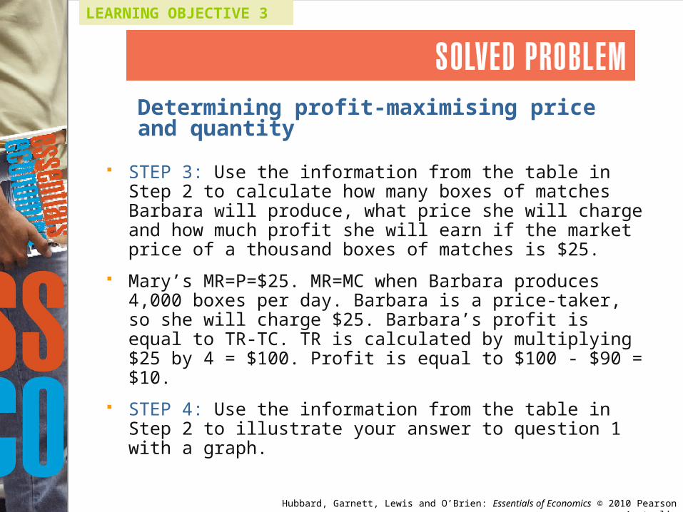
LEARNING OBJECTIVE 3
Determining profit-maximising price and quantity
STEP 3: Use the information from the table in Step 2 to calculate how many boxes of matches Barbara will produce, what price she will charge and how much profit she will earn if the market price of a thousand boxes of matches is $25.
Mary’s MR=P=$25. MR=MC when Barbara produces 4,000 boxes per day. Barbara is a price-taker, so she will charge $25. Barbara’s profit is equal to TR-TC. TR is calculated by multiplying $25 by 4 = $100. Profit is equal to $100 - $90 = $10.
STEP 4: Use the information from the table in Step 2 to illustrate your answer to question 1 with a graph.
Hubbard, Garnett, Lewis and O’Brien: Essentials of Economics © 2010 Pearson Australia
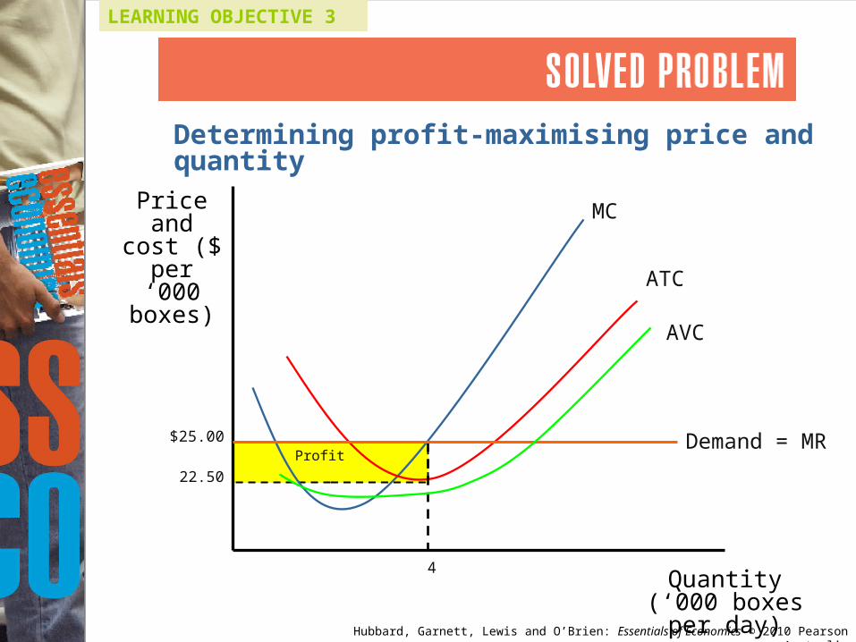
Determining profit-maximising price and quantity
LEARNING OBJECTIVE 3
$25.00
4
ATC
MC
AVC
Demand = MR Profit
22.50
Price and cost ($
per ‘000 boxes)
Quantity (‘000 boxes per day)
Hubbard, Garnett, Lewis and O’Brien: Essentials of Economics © 2010 Pearson Australia
LEARNING OBJECTIVE 3
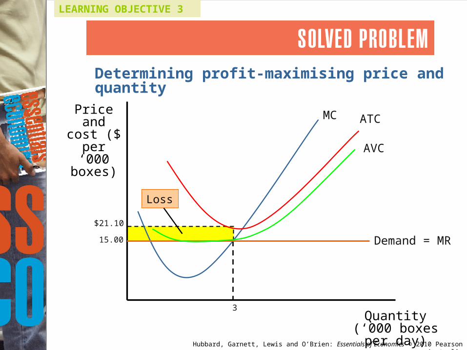
STEP 5: Calculate how many boxes of matches Barbara will produce, what price she will charge and how much profit she will earn if the market price of a thousand boxes of matches is $15.
Referring to the table in Step 2, we can see that MR=MC when Barbara produces 3,000 boxes per day. She charges the market price of $15 per a thousand boxes of matches. Her TR=$15 x 3 = $45, while her TC= $65, so she will have a loss of $20.
Determining profit-maximising price and quantity
Hubbard, Garnett, Lewis and O’Brien: Essentials of Economics © 2010 Pearson Australia
Determining profit-maximising price and quantity
LEARNING OBJECTIVE 3
$21.10
3
ATC MC
AVC
Demand = MR
Loss
15.00
Price and cost ($
per ‘000 boxes)
Quantity (‘000 boxes per day)
Hubbard, Garnett, Lewis and O’Brien: Essentials of Economics © 2010 Pearson Australia
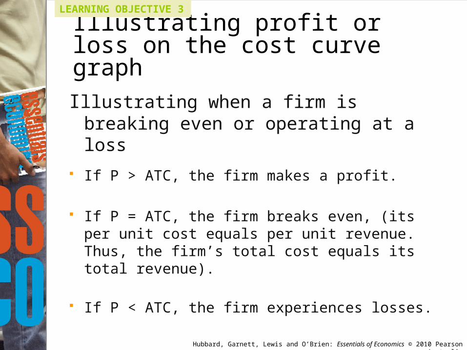
Illustrating profit or loss on the cost curve graph
LEARNING OBJECTIVE 3
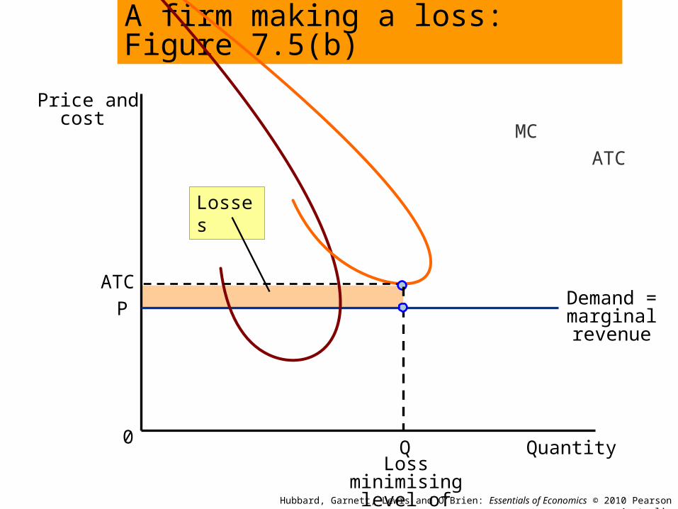
Illustrating when a firm is breaking even or operating at a loss
If P > ATC, the firm makes a profit.
If P = ATC, the firm breaks even, (its per unit cost equals per unit revenue. Thus, the firm’s total cost equals its total revenue).
If P < ATC, the firm experiences losses.
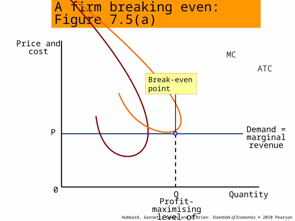
Price and cost
Quantity0
A firm breaking even: Figure 7.5(a)
Hubbard, Garnett, Lewis and O’Brien: Essentials of Economics © 2010 Pearson Australia
Demand = marginal revenue
P
QProfit-maximising
level of output
MC
ATCBreak-even point
Price and cost
Quantity0
A firm making a loss: Figure 7.5(b)
Hubbard, Garnett, Lewis and O’Brien: Essentials of Economics © 2010 Pearson Australia
Demand = marginal revenue
P
QLoss minimising level of output
MC
ATC
Losses
ATC

Hubbard, Garnett, Lewis and O’Brien: Essentials of Economics © 2010 Pearson Australia
Losing money in the medical screening industry
Providing preventive medical scans turned out not to be a profitable business for some entrepreneurs
MAKING THE CONNECTION7.17.1

Hubbard, Garnett, Lewis and O’Brien: Essentials of Economics © 2010 Pearson Australia
Deciding whether to produce or to shut down in the short run
LEARNING OBJECTIVE 4
In the short run a firm suffering losses has two choices: Continue to produce Stop production by shutting down temporarily
Sunk cost: A cost that has already been paid and cannot be recovered.
Hubbard, Garnett, Lewis and O’Brien: Essentials of Economics © 2010 Pearson Australia
LEARNING OBJECTIVE 4
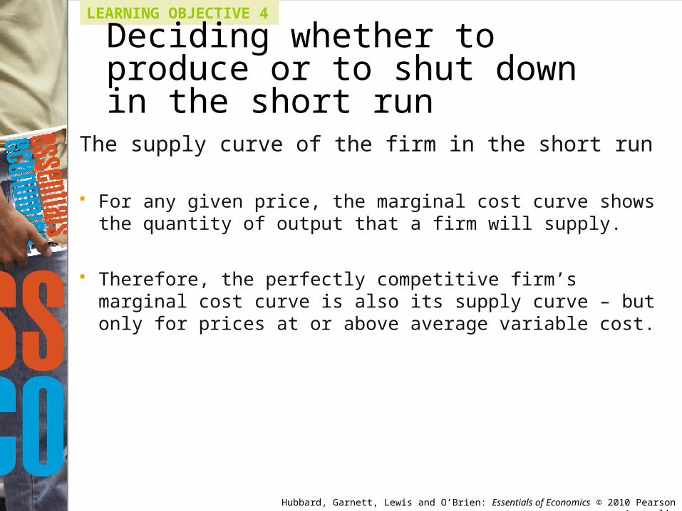
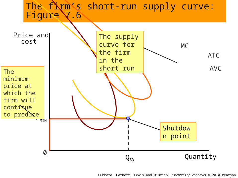
The supply curve of the firm in the short run
For any given price, the marginal cost curve shows the quantity of output that a firm will supply.
Therefore, the perfectly competitive firm’s marginal cost curve is also its supply curve – but only for prices at or above average variable cost.
Deciding whether to produce or to shut down in the short run
Hubbard, Garnett, Lewis and O’Brien: Essentials of Economics © 2010 Pearson Australia
LEARNING OBJECTIVE 4
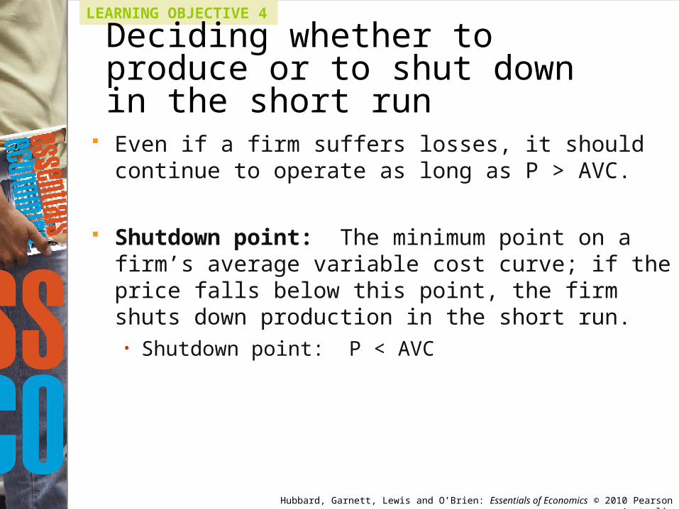
Even if a firm suffers losses, it should continue to operate as long as P > AVC.
Shutdown point: The minimum point on a firm’s average variable cost curve; if the price falls below this point, the firm shuts down production in the short run.• Shutdown point: P < AVC
Deciding whether to produce or to shut down in the short run
Price and cost
Quantity0
The firm’s short-run supply curve: Figure 7.6
Hubbard, Garnett, Lewis and O’Brien: Essentials of Economics © 2010 Pearson Australia
PMIN
QSD
MC
ATC
Shutdown point
AVCThe minimum price at which the firm will continue to produce
The supply curve for the firm in the short run
Hubbard, Garnett, Lewis and O’Brien: Essentials of Economics © 2010 Pearson Australia
LEARNING OBJECTIVE 4
The market supply curve in a perfectly competitive industry
The market supply curve is derived from individual firms’ marginal cost curves.
Deciding whether to produce or to shut down in the short run
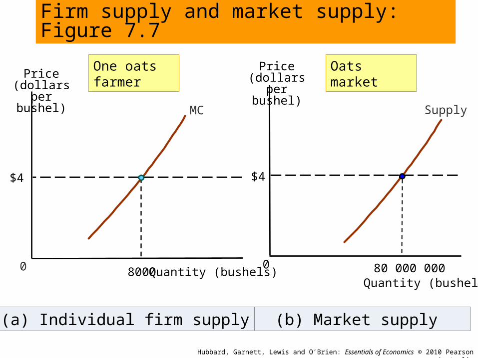
(b) Market supply
0
(a) Individual firm supply
Quantity (bushels)
MC
$4
Firm supply and market supply: Figure 7.7
8000
Price (dollars per bushel)
Price (dollars per bushel)
Quantity (bushels)
0
$4
Hubbard, Garnett, Lewis and O’Brien: Essentials of Economics © 2010 Pearson Australia
Oats marketOne oats farmer
80 000 000
Supply
Hubbard, Garnett, Lewis and O’Brien: Essentials of Economics © 2010 Pearson Australia
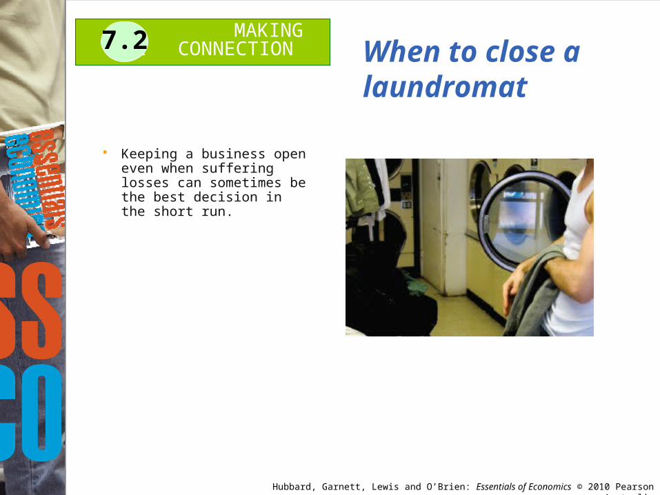
When to close a laundromat
Keeping a business open even when suffering losses can sometimes be the best decision in the short run.
MAKING THE CONNECTION7.2
Hubbard, Garnett, Lewis and O’Brien: Essentials of Economics © 2010 Pearson Australia
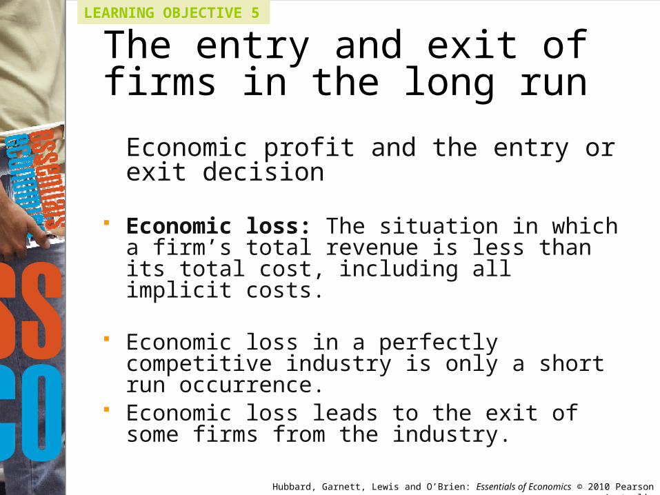
LEARNING OBJECTIVE 5
The entry and exit of firms in the long run
Economic profit and the entry or exit decision
Economic profit: A firm’s revenues minus all its costs, implicit and explicit.
Economic profit in a perfectly competitive industry is only a short run occurrence.
Economic profit leads to the entry of new firms into the industry.
Hubbard, Garnett, Lewis and O’Brien: Essentials of Economics © 2010 Pearson Australia
LEARNING OBJECTIVE 5
The entry and exit of firms in the long run
Economic profit and the entry or exit decision
Economic loss: The situation in which a firm’s total revenue is less than its total cost, including all implicit costs.
Economic loss in a perfectly competitive industry is only a short run occurrence.
Economic loss leads to the exit of some firms from the industry.
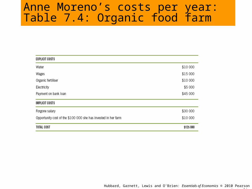
Anne Moreno’s costs per year: Table 7.4: Organic food farm
Hubbard, Garnett, Lewis and O’Brien: Essentials of Economics © 2010 Pearson Australia
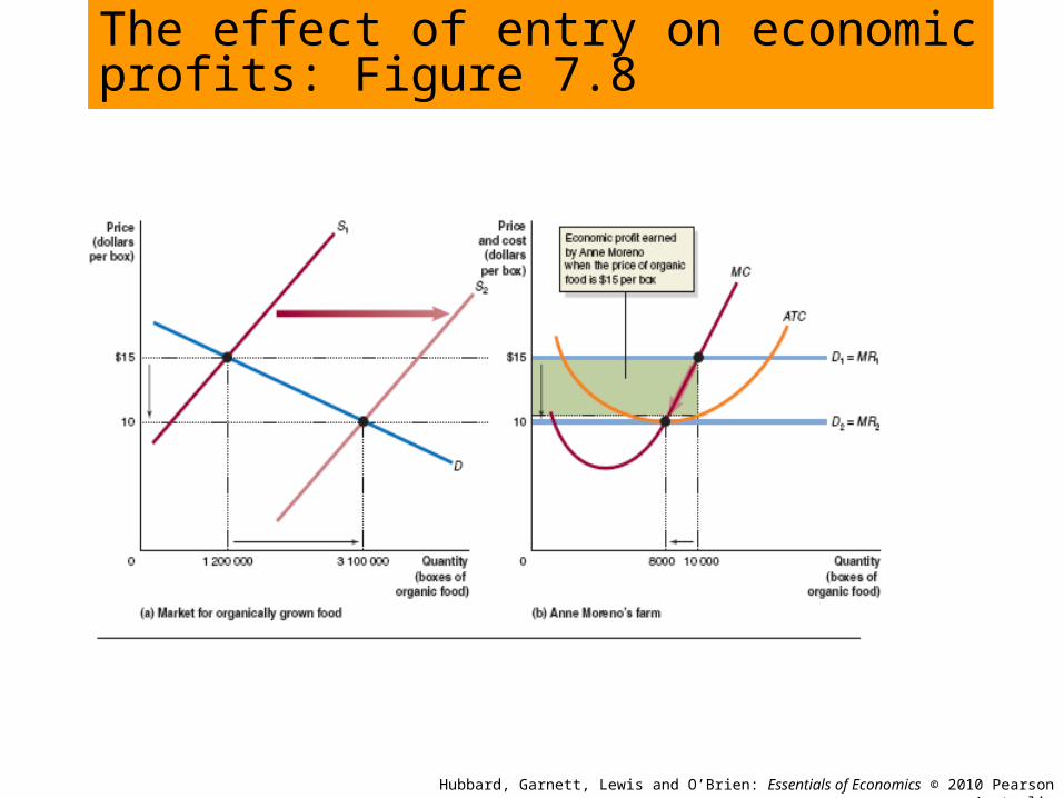
The effect of entry on economic profits: Figure 7.8
Hubbard, Garnett, Lewis and O’Brien: Essentials of Economics © 2010 Pearson Australia
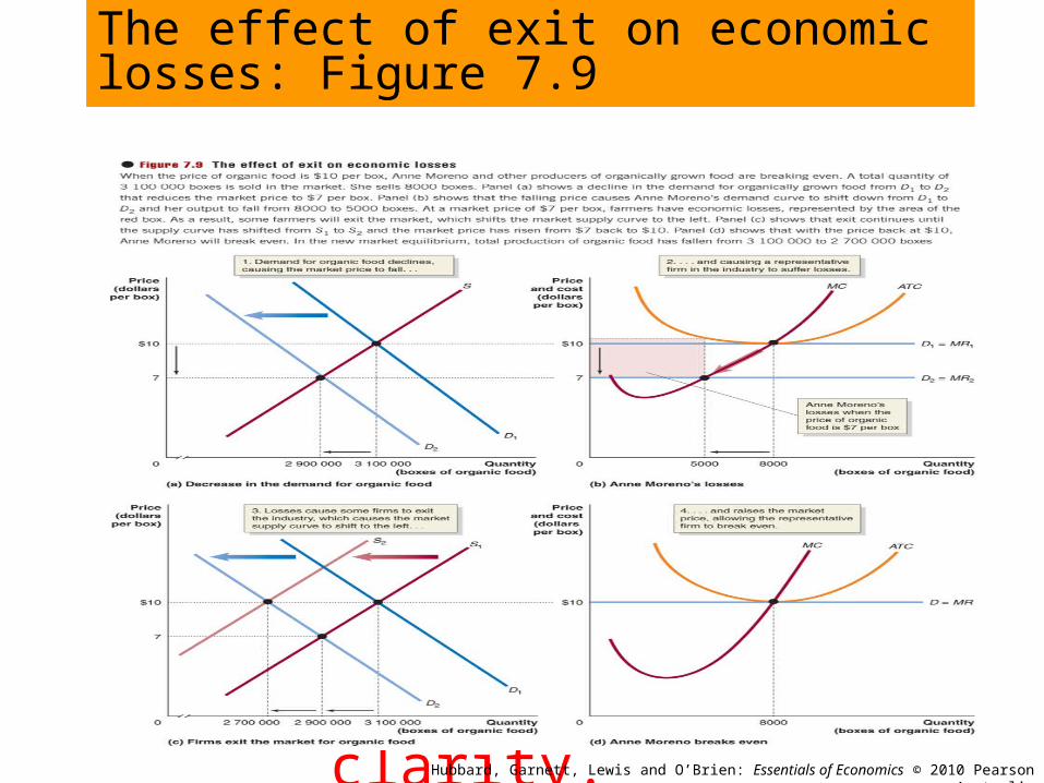
The effect of exit on economic losses: Figure 7.9
Please insert Figure 7.9, (page 208 – top two
graphs) - parts (a) and (b) here, as large as possible, while
maintaining clarity.
Hubbard, Garnett, Lewis and O’Brien: Essentials of Economics © 2010 Pearson Australia
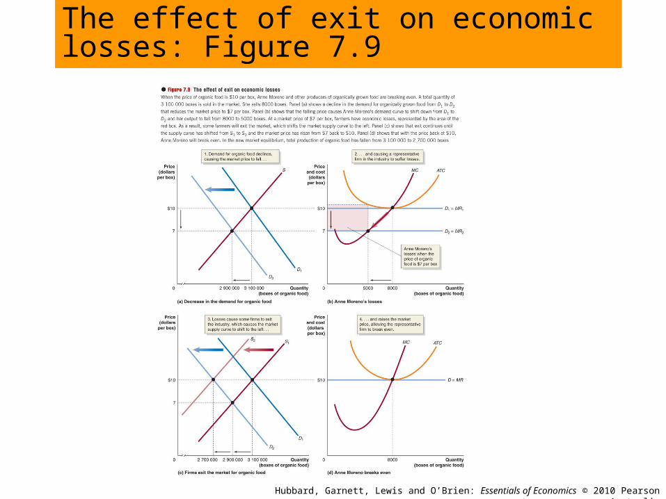
The effect of exit on economic losses: Figure 7.9
Hubbard, Garnett, Lewis and O’Brien: Essentials of Economics © 2010 Pearson Australia
Hubbard, Garnett, Lewis and O’Brien: Essentials of Economics © 2010 Pearson Australia
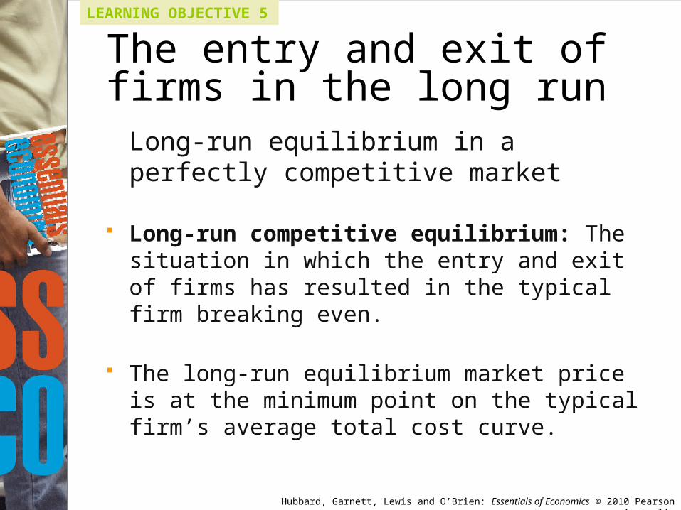
LEARNING OBJECTIVE 5
Long-run equilibrium in a perfectly competitive market
Long-run competitive equilibrium: The situation in which the entry and exit of firms has resulted in the typical firm breaking even.
The long-run equilibrium market price is at the minimum point on the typical firm’s average total cost curve.
The entry and exit of firms in the long run
Hubbard, Garnett, Lewis and O’Brien: Essentials of Economics © 2010 Pearson Australia
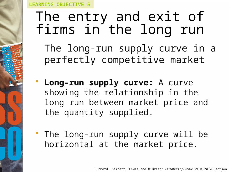
LEARNING OBJECTIVE 5
The long-run supply curve in a perfectly competitive market
Long-run supply curve: A curve showing the relationship in the long run between market price and the quantity supplied.
The long-run supply curve will be horizontal at the market price.
The entry and exit of firms in the long run
Hubbard, Garnett, Lewis and O’Brien: Essentials of Economics © 2010 Pearson Australia
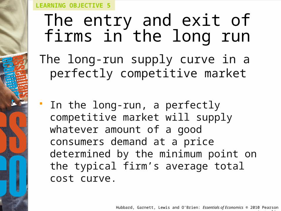
LEARNING OBJECTIVE 5
The long-run supply curve in a perfectly competitive market
In the long-run, a perfectly competitive market will supply whatever amount of a good consumers demand at a price determined by the minimum point on the typical firm’s average total cost curve.
The entry and exit of firms in the long run
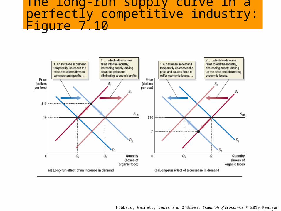
The long-run supply curve in a perfectly competitive industry: Figure 7.10
Hubbard, Garnett, Lewis and O’Brien: Essentials of Economics © 2010 Pearson Australia
Hubbard, Garnett, Lewis and O’Brien: Essentials of Economics © 2010 Pearson Australia
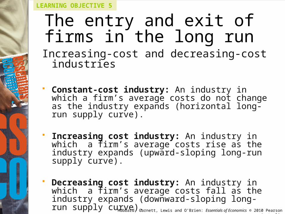
LEARNING OBJECTIVE 5
Increasing-cost and decreasing-cost industries
Constant-cost industry: An industry in which a firm’s average costs do not change as the industry expands (horizontal long-run supply curve).
Increasing cost industry: An industry in which a firm’s average costs rise as the industry expands (upward-sloping long-run supply curve).
Decreasing cost industry: An industry in which a firm’s average costs fall as the industry expands (downward-sloping long-run supply curve).
The entry and exit of firms in the long run
Hubbard, Garnett, Lewis and O’Brien: Essentials of Economics © 2010 Pearson Australia
LEARNING OBJECTIVE 6
Perfect competition and efficiency Productive (technical) efficiency: The
situation in which a given quantity of a good or service is produced using the least amount of resources.
Allocative efficiency: A state of the economy in which production reflects consumer preferences; in particular, every good or service is produced up to the point where the last unit provides a marginal benefit to consumers equal to the marginal cost of producing it.
Hubbard, Garnett, Lewis and O’Brien: Essentials of Economics © 2010 Pearson Australia
LEARNING OBJECTIVE 6
Allocative efficiency Firms will supply all those goods that provide
consumers with a marginal benefit at least as great as the marginal cost of producing them: • The price of a good represents the marginal benefit
consumers receive from the last unit of the good consumed.
• Perfectly competitive firms produce up to the point where the price of the good equals the marginal cost of producing the last unit.
• Therefore, firms produce up to the point where the last unit provides a marginal benefit to consumers equal to the marginal cost of producing it.
Perfect competition and efficiency

Hubbard, Garnett, Lewis and O’Brien: Essentials of Economics © 2010 Pearson Australia
LEARNING OBJECTIVE 6
Dynamic efficiency: The ability of firms over time to develop and utilise technological innovation, and to adapt their product to changes in consumer preferences and tastes.
• When striving for dynamic efficiency, firms will use new technology and thereby reduce production costs (productive efficiency).
• By adapting their product to changes in consumer preferences, firms will produce goods and services consumer value the most (allocative efficiency).
Perfect competition and efficiency

Hubbard, Garnett, Lewis and O’Brien: Essentials of Economics © 2010 Pearson Australia
An Inside Look
Special of the modern day – all organic menu
Hubbard, Garnett, Lewis and O’Brien: Essentials of Economics © 2010 Pearson Australia
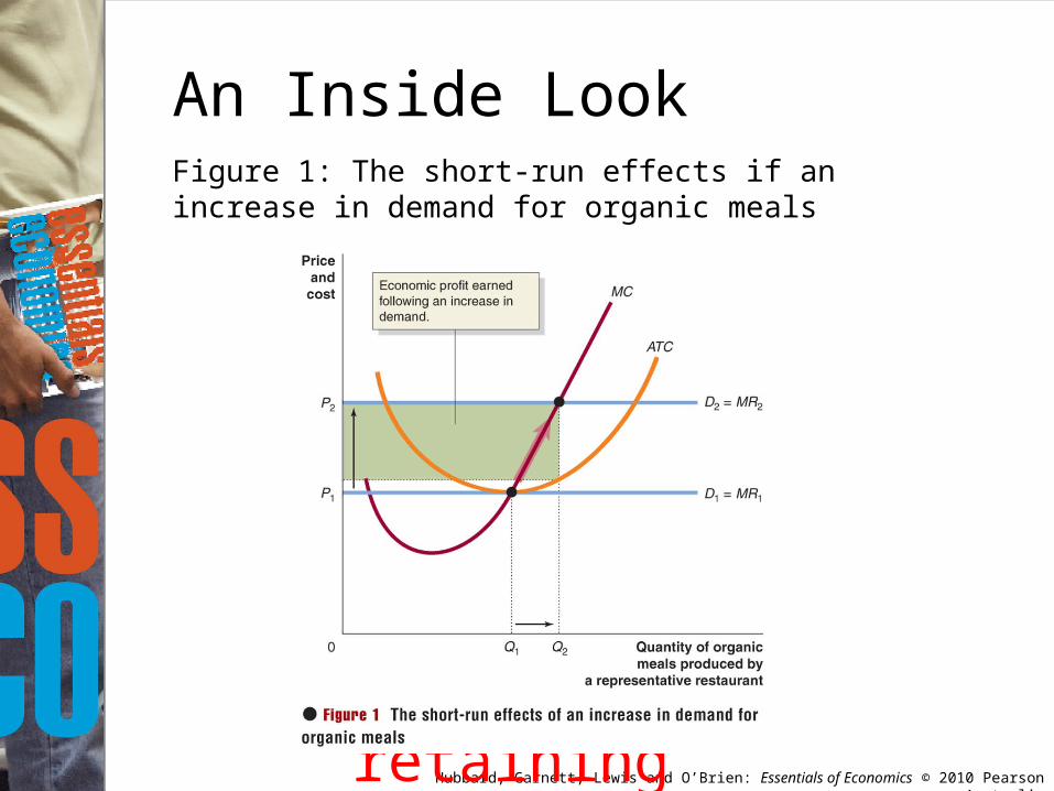
An Inside LookFigure 1: The short-run effects if an increase in demand for organic meals
Insert Figure 1 from page 216, as large as possible
while retaining clarity
Hubbard, Garnett, Lewis and O’Brien: Essentials of Economics © 2010 Pearson Australia
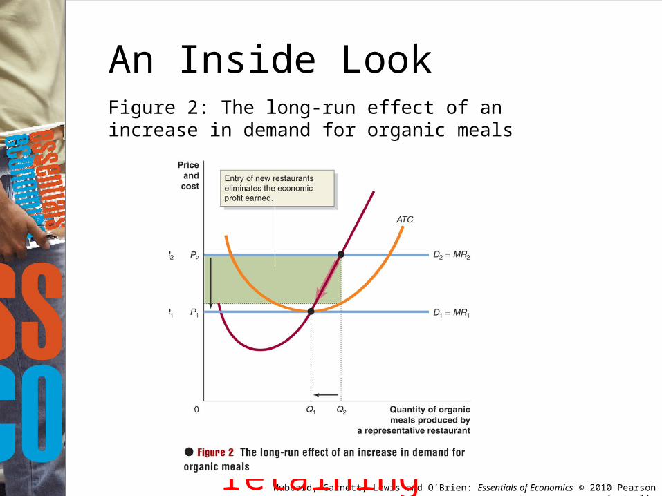
An Inside LookFigure 2: The long-run effect of an increase in demand for organic meals
Insert Figure 2 from page 216, as large as possible
while retaining clarity
Hubbard, Garnett, Lewis and O’Brien: Essentials of Economics © 2010 Pearson Australia
Key Terms Allocative efficiency
Average revenue (AR)
Dynamic efficiency
Economic loss
Economic profit
Long-run competitive equilibrium
Long-run supply curve
Marginal revenue (MR)
Perfectly competitive market
Price taker
Productive (technical) efficiency
Profit
Shutdown point
Sunk cost
Hubbard, Garnett, Lewis and O’Brien: Essentials of Economics © 2010 Pearson Australia
Get Thinking!
A single desk arrangement for wheat exports was in place in Australia for more than 60 years. The Australian Wheat Board (AWB) purchased wheat from farmers at fixed prices and sold it on international markets. Effectively, Australian wheat growers operated under the conditions extremely close to perfect market competition where they were effectively price-takers.
This single desk arrangement was scrapped on 30/06/2008.
How much do you think this change will affect wheat farmers in terms of the price they will be able to charge for their wheat?
http://www.pc.gov.au/research/submission/wheat1
Hubbard, Garnett, Lewis and O’Brien: Essentials of Economics © 2010 Pearson Australia
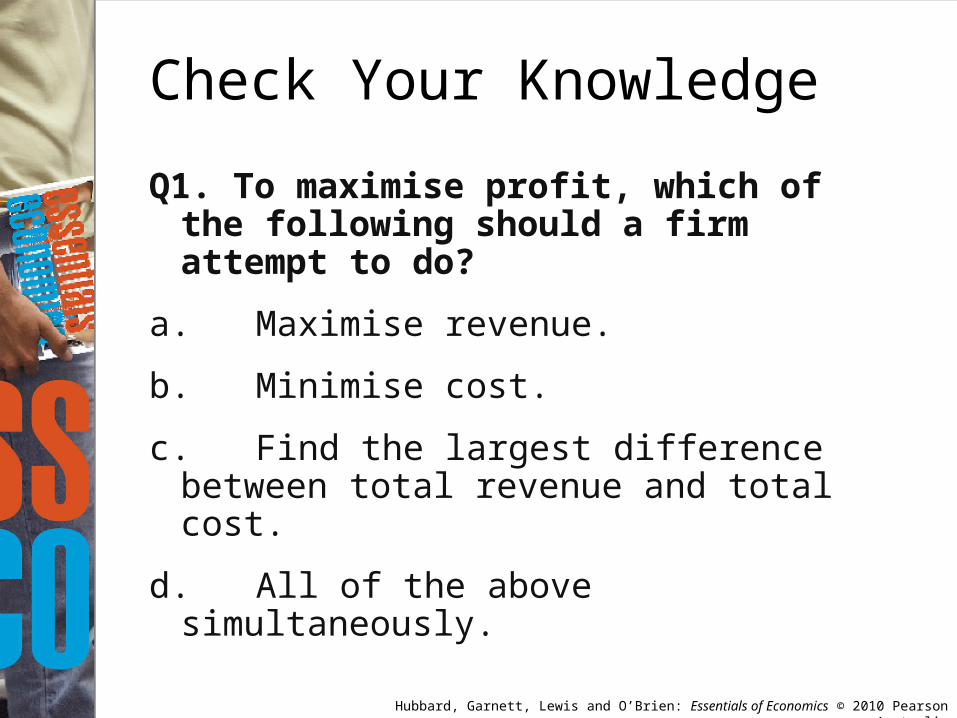
Check Your Knowledge
Q1. To maximise profit, which of the following should a firm attempt to do?
a. Maximise revenue.
b. Minimise cost.
c. Find the largest difference between total revenue and total cost.
d. All of the above simultaneously.
Hubbard, Garnett, Lewis and O’Brien: Essentials of Economics © 2010 Pearson Australia
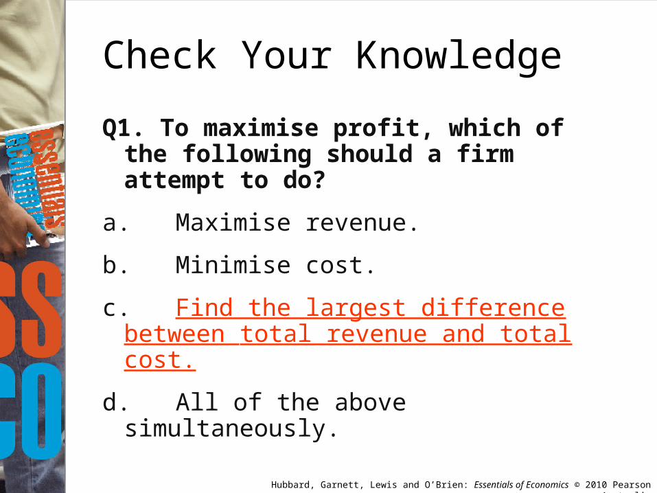
Check Your Knowledge
Q1. To maximise profit, which of the following should a firm attempt to do?
a. Maximise revenue.
b. Minimise cost.
c. Find the largest difference between total revenue and total cost.
d. All of the above simultaneously.
Hubbard, Garnett, Lewis and O’Brien: Essentials of Economics © 2010 Pearson Australia
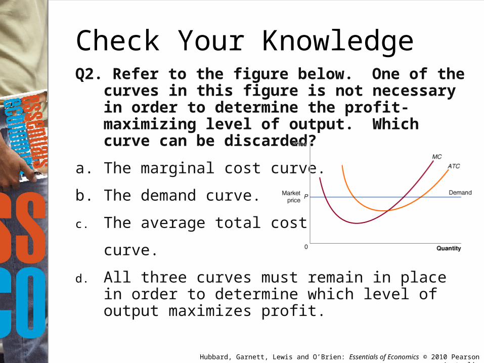
Check Your KnowledgeQ2. Refer to the figure below. One of the curves in
this figure is not necessary in order to determine the profit-maximizing level of output. Which curve can be discarded?
a. The marginal cost curve.
b. The demand curve.
c. The average total cost
curve.
d. All three curves must remain in place in order to determine which level of output maximizes profit.
Hubbard, Garnett, Lewis and O’Brien: Essentials of Economics © 2010 Pearson Australia
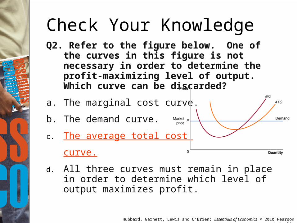
Check Your KnowledgeQ2. Refer to the figure below. One of the curves in
this figure is not necessary in order to determine the profit-maximizing level of output. Which curve can be discarded?
a. The marginal cost curve.
b. The demand curve.
c. The average total cost
curve.
d. All three curves must remain in place in order to determine which level of output maximizes profit.
Hubbard, Garnett, Lewis and O’Brien: Essentials of Economics © 2010 Pearson Australia
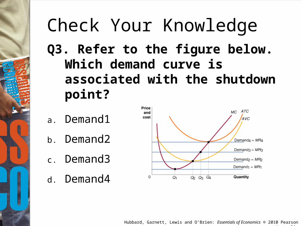
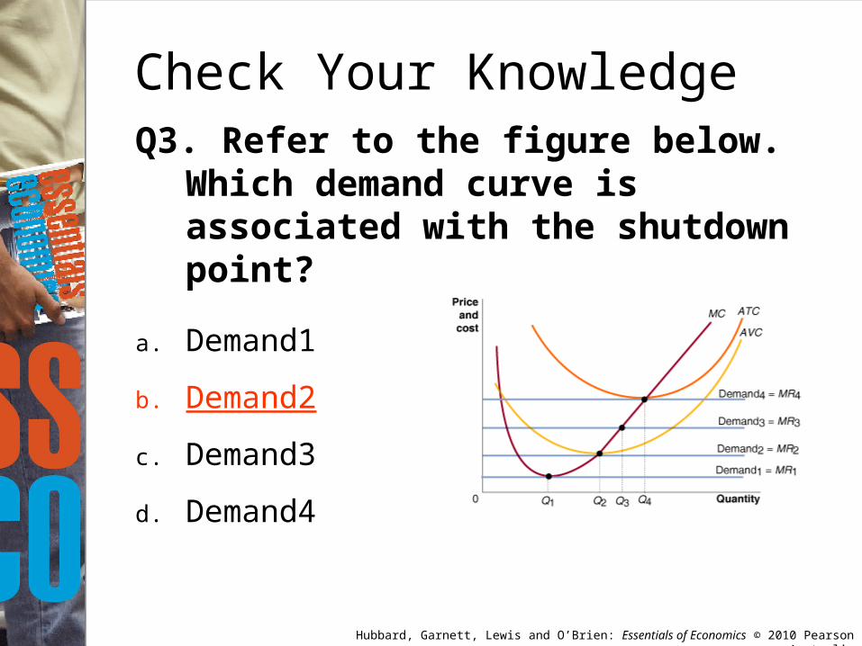
Q3. Refer to the figure below. Which demand curve is associated with the shutdown point?
a. Demand1
b. Demand2
c. Demand3
d. Demand4
Check Your Knowledge
Hubbard, Garnett, Lewis and O’Brien: Essentials of Economics © 2010 Pearson Australia
Q3. Refer to the figure below. Which demand curve is associated with the shutdown point?
a. Demand1
b. Demand2
c. Demand3
d. Demand4
Check Your Knowledge
Hubbard, Garnett, Lewis and O’Brien: Essentials of Economics © 2010 Pearson Australia
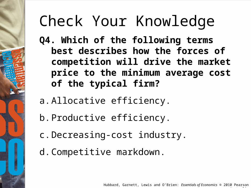
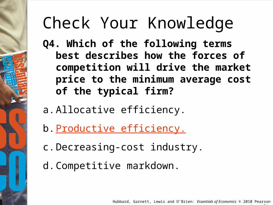
Q4. Which of the following terms best describes how the forces of competition will drive the market price to the minimum average cost of the typical firm?
a. Allocative efficiency.
b. Productive efficiency.
c. Decreasing-cost industry.
d. Competitive markdown.
Check Your Knowledge
Hubbard, Garnett, Lewis and O’Brien: Essentials of Economics © 2010 Pearson Australia
Q4. Which of the following terms best describes how the forces of competition will drive the market price to the minimum average cost of the typical firm?
a. Allocative efficiency.
b. Productive efficiency.
c. Decreasing-cost industry.
d. Competitive markdown.
Check Your Knowledge


