POWERSDR USER NOTES - Software-defined...

POWERSDR™/OPENHPSDR USER NOTES Page 1

POWERSDR™/OPENHPSDRUSERNOTESThis document is intended to describe the operation of certain PowerSDR™ features that are unique to

HPSDR or have been modified / improved and operate differently on HPSDR hardware than on other

hardware platforms.

TableofContentsPOWERSDR™/OPENHPSDR USER NOTES ...................................................................................................... 1

AGC – Automatic Gain Control (NR0V, 2012‐11‐23) ..................................................................................... 2

The Basics .................................................................................................................................................. 2

AGC Presets ............................................................................................................................................... 2

Panadapter Controls ................................................................................................................................. 3

Custom Settings ........................................................................................................................................ 3

Gain Details / Example .............................................................................................................................. 3

AM/SAM – Demodulation (NR0V, revised 2013‐03‐07) ............................................................................... 4

AM – Modulation (NR0V, 2014‐05‐22) ......................................................................................................... 5

Automatic Noise Reduction (NR0V, 2012‐10‐07) ......................................................................................... 5

Automatic Notch Filter (NR0V, 2012‐10‐07) ................................................................................................. 6

Transmit ALC (NR0V, 2014‐05‐22) ................................................................................................................ 6

Noise Blanker (NR0V, 2014‐05‐22) ............................................................................................................... 7

Introduction .............................................................................................................................................. 7

NB .............................................................................................................................................................. 7

NB2 ............................................................................................................................................................ 8

Adjusting the Noise Blankers .................................................................................................................. 10

Panadapter – Deep and Wide FFTs (NR0V, revised 2013‐04‐06) ............................................................... 10

Introduction ............................................................................................................................................ 10

Controls ................................................................................................................................................... 11

FFT Size & Sample Rate ........................................................................................................................... 12

Lowering the Noise Floor ........................................................................................................................ 12

384K Operation – Some Considerations (NR0V – 2013‐02‐21) .................................................................. 13


AGC–AutomaticGainControl(NR0V,2012‐11‐23)

TheBasicsReceived signals may vary in strength by several orders of magnitude. The AGC automatically adjusts

the gain applied to signals such that the audio volume is relatively constant independent of the of the

received signal strength. To maintain excellent audio quality, gain changes are not instantaneous; gain

changes follow exponential curves defined by time constants. Gain changes LEAD changes in received

signal strength—this ensures that the audio output never overshoots or undershoots the appropriate

levels.

This is a single‐attack, dual‐decay system meaning that a single time constant is used to decrease the

gain and two different time constants are available to increase the gain. The attack time constant and

the normal‐decay time constant are user selectable while the fast‐decay time constant is set as an

internal parameter. The fast‐decay time constant is employed following a fast impulse, i.e., a noise

“spike”, so as to prevent the AGC from blocking a weak signal during the time‐span of a normal‐decay

from the transient.

“Hang” functionality is incorporated to delay an increase in gain in certain situations, for example during

a brief pause in speech of a strong SSB station. This maintains quieting during the pause by holding the

gain constant during the hang‐time.

Gain Slope functionality allows a user‐selectable amount of gain above the “knee” or “threshold” at

which the AGC begins to limit gain. This allows, for example, a very strong signal to sound somewhat

louder than a strong signal.

AGCPresetsSeveral presets are found under the AGC pull‐down on the radio front‐panel.

Fixed: AGC is turned OFF. The gain is fixed rather than the AGC automatically adjusting it. The

Fixed Gain adjustment appears in place of AGC Gain on the front‐panel. Use care when

switching to this mode! With no gain reduction applied by the AGC, very high volumes can

result depending upon the Fixed Gain Setting.

Long: The attack time‐constant is 2ms; the normal decay time‐constant is 2000ms, hang is

enabled with a hang time of 2000ms. Note that the “time‐constants” are really that, i.e., it takes

several time constants for complete gain adjustment. The hang‐time is NOT a time‐constant, it

is a fixed time.

Slow: Attack τ = 2ms; Normal Decay τ = 500ms; Hang Time t = 1000ms.

Medium: Attack τ = 2ms; Normal Decay τ = 250ms; Hang is DISABLED.

Fast: Attack τ = 2ms; Normal Decay τ = 50ms; Hang is DISABLED.

Custom: Uses the “custom” settings on Setup Form ‐> DSP ‐> AGC/ALC.


PanadapterControlsThere are two controls that can be enabled to appear directly on the panadapter—AGC Max Gain and

Hang Threshold. The controls can be enabled in “Setup Form ‐> DSP ‐> AGC/ALC”. Note, however, that

the HANG is permanently disabled and will not appear in certain of the AGC Presets.

The AGC Max Gain is the maximum gain that the AGC will apply to increase the strength of a signal. This

operates somewhat like the RF Gain of an analog radio. By grabbing the box at the left‐end of the “G”

line, one would normally set this level a bit above the noise floor on the panadapter.

The “H” line is to set the hang threshold. If a signal has sufficient strength to cross the H line, a hang will

be invoked. Moving this line to the top of the screen effectively disables Hang.

CustomSettingsUnder “Setup Form ‐> DSP ‐> AGC/ALC”, the attack and normal‐decay time‐constants, hang‐time, hang‐

threshold (also on the panadapter), Maximum AGC Gain (also on the panadapter and front‐panel), and

slope can be independently adjusted.

Slope has a range of 0dB to 20dB. At 0dB, there is no slope and all signals will be limited to the same

output level. At 20dB of slope, an extremely strong signal could produce 20dB higher output volume

than a signal just meeting the AGC threshold. Settings of 6dB to 10dB may be preferable.

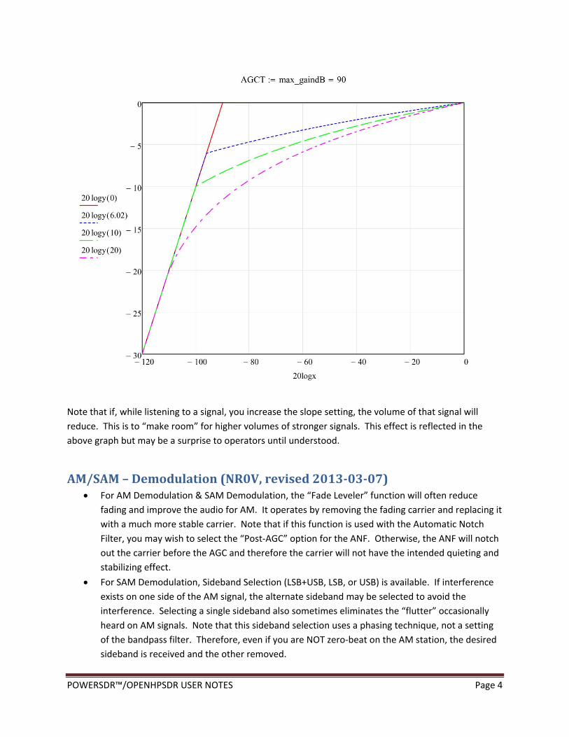
GainDetails/ExampleFor those who really want to understand how the AGC controls gain, the following example is provided.

Shown below is the gain response (output versus input) for this system with an AGC Gain setting of

90dB. Four different potential output responses are shown corresponding to four different Slope

settings. The Slope settings are the values in parenthesis for each output curve.

Note that, in each case, the Slope setting is the amount of available gain between the knee of the curve

and the maximum output level. All curves converge at the maximum output level at the upper right

corner of the graph.

As noted above, in this example, AGC Max Gain is set to 90dB. This value represents the gain below the

respective knee of each curve. The 0dB‐slope curve clearly displays that, at an input of ‐90dB, the

output is 0dB, i.e., there’s 90dB gain.


Note that if, while listening to a signal, you increase the slope setting, the volume of that signal will

reduce. This is to “make room” for higher volumes of stronger signals. This effect is reflected in the

above graph but may be a surprise to operators until understood.

AM/SAM–Demodulation(NR0V,revised2013‐03‐07) For AM Demodulation & SAM Demodulation, the “Fade Leveler” function will often reduce

fading and improve the audio for AM. It operates by removing the fading carrier and replacing it

with a much more stable carrier. Note that if this function is used with the Automatic Notch

Filter, you may wish to select the “Post‐AGC” option for the ANF. Otherwise, the ANF will notch

out the carrier before the AGC and therefore the carrier will not have the intended quieting and

stabilizing effect.

For SAM Demodulation, Sideband Selection (LSB+USB, LSB, or USB) is available. If interference

exists on one side of the AM signal, the alternate sideband may be selected to avoid the

interference. Selecting a single sideband also sometimes eliminates the “flutter” occasionally

heard on AM signals. Note that this sideband selection uses a phasing technique, not a setting

of the bandpass filter. Therefore, even if you are NOT zero‐beat on the AM station, the desired

sideband is received and the other removed.


A “DC Block” option has been added on the Setup/DSP/AM‐SAM tab. This option removes the

carrier from the signal at the end of the audio processing chain. When doing WAV

record/playback in the AM/SAM modes, this option is recommended. Also, under

Wave_File_Controls/Options, select Receive “Post‐Processed Audio.”

AM–Modulation(NR0V,2014‐05‐22) The carrier level control on the Transmit setup tab adjusts the ratio of carrier to audio.

o The normal setting is 100.0. At this level, assuming sufficient mic gain, you will achieve

100% modulation. The ALC limits the audio such that you will not exceed 100%

modulation. At this setting, with no modulation, the ALC meter should show ‐6dB.

o When another station is receiving you with a synchronous detector, you may be able to

reduce the carrier level and, assuming sufficient signal strength, the synchronous

detector may still be able to lock on the signal and demodulate it correctly. Note that

this reduction in carrier will produce distortion on a normal AM detector. At a carrier

level of 0, you have no carrier, i.e., you are transmitting DSB.

o If you wish to modulate at less than 100%, increase the carrier level above 100. The ALC

will reduce the audio accordingly such that the total signal remains with the limits

required by the HPSDR transmitter card.

Note that the modulation algorithm prevents “carrier shift.” This means that the carrier level

will NOT vary based upon the level of the modulation.

AutomaticNoiseReduction(NR0V,2012‐10‐07) Expectations:

o LMS Noise Reduction algorithms work best when the signals already have a good signal‐

to‐noise ratio; they can be very effective in providing a quiet background under these

circumstances. This is really their purpose.

o It is unlikely that you will be able to pull an otherwise unreadable signal out of the noise

with this type algorithm.

o This algorithm is CPU intensive. The CPU load increases with the number of taps and

with sample rate.

Use:

o Set the AGC Gain line just above the noise floor for best operation. (So AGC doesn’t

undo what the ANR is trying to do.)

o Baseline values to try FOR 192K SAMPLE RATE:

Taps = 256 (increase to expand frequency range, generally reduces noise)

Delay = 64 (generally increase to reduce noise)

Gain = 100* (decrease to reduce noise)


Leak = 100 (Increase to reduce noise)

*Lower values of gain may work very well on CW signals.

o The Pre‐AGC position in the processing pipeline should generally be used. Post‐AGC

may work better in certain situations, for example, fast QSB.

AutomaticNotchFilter(NR0V,2012‐10‐07) Expectations:

o This algorithm is CPU intensive. The CPU load increases with the number of taps and

with sample rate.

o Increasing gain allows the algorithm to more effectively lock onto and notch carriers.

HOWEVER, at higher gains the algorithm will begin to generate distortion on speech.

I.e., there is a tradeoff between notching effectiveness and speech distortion.

Use:

o Baseline values to try FOR 192K SAMPLE RATE:

Taps = 256 (increase to expand effective frequency range)

Delay = 64 (lower to increase maximum effective frequency)

Gain = 200 (increase to more effectively lock onto carriers)

Leak = 100

o The Pre‐AGC position in the processing pipeline should generally be used. Post‐AGC

may work better in certain situations, for example, fast QSB, or when listening to AM

with the Fade Leveler enabled.

TransmitALC(NR0V,2014‐05‐22) WITH MORE RECENT VERSIONS OF OUR SOFTWARE, ALC IS PERMANENTLY ENABLED.

With HPSDR, it is necessary to limit the signal transferred to the transmitter hardware to below

a particular level; otherwise, very broadband splatter can result. The transmit ALC does this

limiting.

Proper operation of the ALC is indicated by the fact that the ALC Meter will not exceed 0dB.

Normal settings for ALC parameters are:

o Attack = 2ms

o Decay = 10ms

o Hang = 500ms


NoiseBlanker(NR0V,2014‐05‐22)

IntroductionNoise Blankers are used to remove "impulse" noise. Impulse noise consists of brief bursts or noise often

generated by arcing power line insulators, electric motors, automotive ignitions, etc. In the case of

impulse noise related to electrical power lines and appliances, the impulses often occur at the power

line frequency or a multiple thereof. Research has shown that the duration of these impulses is rarely

more than 3mS to 5mS and that they can be much shorter. These impulses are often much larger in

amplitude that the signal we are trying to receive; therefore, they are very disruptive to reception.

The basic concept of a noise blanker is to replace the signal during the impulses with either zero or some

value much more representative of what the signal should be. The noise blanker algorithm depends

upon the fact that the impulses are much larger than the signal to be able to detect them. It compares

the signal at each sample with the long‐term average value across a wide bandwidth. If the samples

exceed a "Threshold" referenced to the average, it concludes this is an impulse.

There are currently two noise blankers in OpenHPSDR mRX PS as of the 3.2.11 release. The basic noise

blanker "NB" has been there since February 2013. The new "NB2" is EXPERIMENTAL and feedback

would be appreciated.

More details on each of these noise blankers are given below.

NBThe console “NB” button activates the basic NB noise blanker. The noise blanker is used to remove

short noise bursts from the stream of signal samples. To capture the noise bursts as completely as

practical and to minimize damage to the frequency spectrum in the process, this algorithm operates as

follows:

1. It “looks ahead” to see if a noise burst is coming.

2. When there’s a burst on the horizon, the signal level is gradually decreased, in a controlled

fashion, to zero. The time from full signal to zero signal is “Slew” time.

3. The signal is held at zero for a “Lead” time before the burst arrives to catch as much as practical

of the burst leading edge.

4. The signal is held at zero during the pulse and for “Lag” time after the pulse to catch as much as

practical of the trailing edge.

5. The signal is then restored to full value using a controlled transition in “Transition” time.

The times (Transition, Lead, and Lag) as well as the Noise Blanker Threshold are all adjustable on the

DSP/Options setup tab.

The following image taken from a simulation helps visualize what’s happening. The blue signal is the

input to the noise blanker and the red signal is the output.


“Threshold” sets the peak level at which the input amplitude is judged to be a noise burst rather than

just a signal. Therefore, if you set Threshold too low, you will begin to cut out normal signals. If you set

Threshold too high, you won’t catch the noise burst.

Suggested settings for the times are all 0.1ms. However, if your particular noise problem is still partially

sneaking through, try increased values.

NB2NB2 is considered EXPERIMENTAL at this point. I am interested in feedback as to whether you have

impulse noise that can be more effectively removed by NB2 than by NB. If such cases are not found, I

will likely remove this code in some future release.

NB2 supports five modes of operation:

Zero ‐ When an impulse is detected, for the duration of the impulse, the output signal is zeroed.

Sample‐Hold ‐ When an impulse is detected, for the duration of the impulse, the output signal is

held at the value occurring just before the impulse. (This mode is basically the same as the

"legacy" NB2 blanker that was in PowerSDR some years ago.)

Hold‐Sample ‐ When an impulse is detected, for the duration of the impulse, the output signal is

held at the value occurring just after the impulse.

Mean‐Hold ‐ When an impulse is detected, for the duration of the impulse, the output signal is

held at the mean of the values occurring just before and just after the impulse.

Linear ‐ When an impulse is detected, during the impulse the output signal is a linear

interpolation from the signal value occurring just before the impulse and the signal value just

after the impulse.


Three of the five modes require knowing the value of the signal AFTER the impulse. To accomplish this,

a delay line is required. Hence, a finite latency is introduced in the processing chain. Literature and

other current information indicates that impulses are usually less than 5 mS. However, to be

conservative, a 25 mS impulse length is currently supported.

As the noise impulses will not have perfect vertical edges, some additional provisions are made to blank

during these ragged edges before and after the impulse is of such a magnitude as to be clearly detected

as an impulse, i.e., before and after the "primary impulse period."

Advance Slew ‐ In advance of an impulse, a raised‐cosine slew is performed from a known point

on the signal waveform to the "initial blanking value." Except for the Zero and Hold‐Sample

modes, the initial blanking value is dependent upon a pre‐impulse signal value (now perhaps

getting into the edge of the impulse) that is calculated using a 10‐coefficient FIR filter looking at

preceding samples.

Advance ‐ Between the Advance Slew and the primary impulse period, an advance period can be

specified. The advance period will become part of the blanking interval, i.e., behavior during

this period will be just as during the primary impulse period.

Hang ‐ After the detected impulse, a hang period can be specified. The hang period will become

part of the blanking interval, i.e., behavior during this period will be just as during the primary

impulse period.

Hang Slew ‐ After an impulse, a raised‐cosine slew is performed from the "final blanking value"

to a known point on the signal waveform. Except for Zero and Sample‐Hold modes, the final

blanking value is dependent upon a post‐impulse signal value (perhaps still in the edge of the

impulse) that is calculated using a 10‐coefficient FIR filter looking at following samples.

If the combination of Advance Slew, Advance, Hang, and Hang Slew completely bridge the time between

multiple impulses, that impulse‐sequence will be treated as a single impulse. If an impulse or connected

impulse sequence exceeds the capacity of the delay line, Zero mode is used since the signal value at the

end of the impulse/sequence is unknown and the impulse is of such length that the intervening signal is

likely to be closer to zero, on average, than to the sample‐hold value.

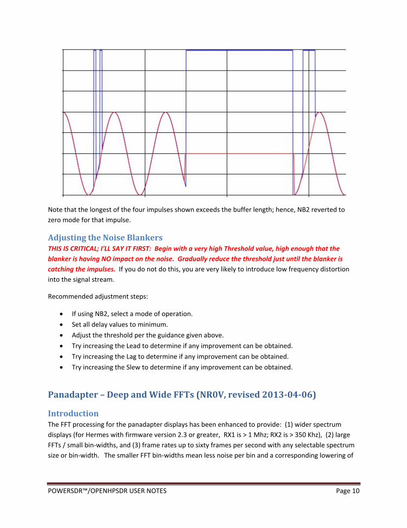
As an example, here's a view (from simulation) of how the blanker behaves operating in "Linear" mode.


Note that the longest of the four impulses shown exceeds the buffer length; hence, NB2 reverted to

zero mode for that impulse.

AdjustingtheNoiseBlankersTHIS IS CRITICAL; I'LL SAY IT FIRST: Begin with a very high Threshold value, high enough that the

blanker is having NO impact on the noise. Gradually reduce the threshold just until the blanker is

catching the impulses. If you do not do this, you are very likely to introduce low frequency distortion

into the signal stream.

Recommended adjustment steps:

If using NB2, select a mode of operation.

Set all delay values to minimum.

Adjust the threshold per the guidance given above.

Try increasing the Lead to determine if any improvement can be obtained.

Try increasing the Lag to determine if any improvement can be obtained.

Try increasing the Slew to determine if any improvement can be obtained.

Panadapter–DeepandWideFFTs(NR0V,revised2013‐04‐06)

IntroductionThe FFT processing for the panadapter displays has been enhanced to provide: (1) wider spectrum

displays (for Hermes with firmware version 2.3 or greater, RX1 is > 1 Mhz; RX2 is > 350 Khz), (2) large

FFTs / small bin‐widths, and (3) frame rates up to sixty frames per second with any selectable spectrum

size or bin‐width. The smaller FFT bin‐widths mean less noise per bin and a corresponding lowering of


the noise floor for viewing weaker signals. The higher frame rates provide a more pleasing display as

well as the opportunity to catch transient signals that may be missed with infrequent display updates.

These new capabilities come with some costs: (1) added memory utilization to store the additional

samples required, and (2) an increase in CPU processing requirements. The additional memory is

allocated when PowerSDR mRX is opened. However, the amount of additional CPU processing (if any) is

dependent upon YOUR user settings. You can minimize CPU utilization by restricting your operation to

the FFT depth and width limits that were in place prior to these enhancements, specifically: (1) use the

minimum FFT size, and (2) restrict your spectrum view to less than ~188Khz. Also, you can reduce your

frame rate as the FFT computations performed are directly proportional to the specified frame rate.

Averaging of multiple FFT results is useful to reduce the instantaneous noise. Five averaging modes are

now available:

1. “Weighted – Log” averaging weights recent FFTs more heavily than older FFTs; however, no FFTs

are ever completely removed from the average. This average is done after the data is converted

to the log(dB) scale which is displayed. Therefore, the averaging appears “natural” on the

displayed log scale. The relative weights of new versus older FFTs depend upon the

Averaging/Time setting.

2. “Weighted – Linear” averaging operates similarly to “Weighted – Log”; however, it averages the

FFT data before it is converted to the log scale. This has the interesting property of displaying a

reasonable representation of peak values while still averaging to calm the noise floor.

3. “Window – Log” averaging operates on the data after the conversion to the log scale; however,

it equally weights the last N FFTs, where N depends upon the Averaging/Time setting. In this

way, old FFTs are completely dropped from the average as they move outside the time window.

4. “Window – Linear” averaging operates similarly to “Window – Log”; however, it averages the

FFT data before it is converted to the log scale.

5. “Low Noise Floor” averaging operates similarly to “Weighted – Log”; however, it re‐orders

operations so as to reduce the noise floor by an extra one to two dB. CAUTION: This mode uses

considerably more CPU cycles, especially if zoomed out such that a large spectrum is visible.

With larger FFT sizes and high frame rates, the averaging controls will have much less effect on the

display.

Note that very large FFTs will produce displays that seem to move in slow motion. This occurs because

the time window to capture the required number of samples for the FFTs is much larger.

ControlsMost controls are exactly the same as before, however, new setup tabs with additional controls are

provided for RX1, RX2, and TX:

Setup/General/Hardware Config: Checking the Limit Receivers/2‐Receivers box will limit the

panadapter bandwidth to slightly less than the chosen sample_rate thereby reducing use of

CPU cycles. Note that you can get approximately the same reduction in CPU cycles by just


zooming in to restrict your viewed bandwidth. However, checking this box will also reduce your

network bandwidth requirement.

Console: The Zoom control works as before—but with extended range for Hermes users.

Console: The Pan control works as before.

Console: The AVG button turns averaging ON and OFF.

Console: The Peak button turns peak capture mode ON and OFF.

Setup/Display/RX1 and Setup/Display/RX2: Averaging/Time controls the timing for your choice

of Averaging modes.

Setup/Display/RX1 and Setup/Display/RX2: There are seven FFT sizes selectable using a slider.

The corresponding bin‐width is displayed.

Setup/Display/RX1 and Setup/Display/RX2: The Window function for the FFT is selectable.

Window functions control the leakage among frequency bins and result in variation in other

properties of the display. For example, the Flat‐top window offers exceptional amplitude

accuracy while the Kaiser window is an excellent choice for general use.

Setup/Display/TX: Window selection is provided.

Setup/Display/TX: Polyphase may be enabled to slightly improve the resolution of frequencies.

FFTSize&SampleRateNote that bin‐width is a function of BOTH the FFT Size AND the Sample Rate chosen in Setup/Audio.

Larger FFT sizes of course produces smaller bin widths. Lower sample rates also produce smaller bin

widths. However, lower sample rates mean that it takes longer to collect the samples and the display

response will be correspondingly slower. The displayable spectrum is also proportional to the chosen

sample rate.

LoweringtheNoiseFloor

Use large FFT sizes and low sample rates. Choose the “Low Noise Floor” averaging mode. Zoom IN as much as practical per your needs.


384KOperation–SomeConsiderations(NR0V–2013‐02‐21)

384K has now been added as a sample‐rate option for Hermes users. 384K allows wider spectrum

displays and more range for sub‐receivers. However, processing more samples per second and

achieving processing quality equivalent to that at lower sample rates require more CPU cycles and more

memory for sample storage.

When increasing sample rate, you may want to consider your other settings in several areas.

DSP Buffer Sizes – When you increase the sample rate, the cut‐off of receive and transmit band‐

pass filters will be less sharp/defined unless you also increase the DSP buffer size. To allow you

this option, two new DSP buffer sizes (8192 and 16384) have been provided as possible

selections. Note that you can check your filter roll‐off using the “Spectrum” display option.

Automatic Notch Filter – To achieve the same frequency coverage, you may wish to increase the

number of taps and delay settings when moving to a higher sample rate. The available ranges

have been expanded.

Noise Reduction ‐ To achieve the same frequency coverage, you may wish to increase the

number of taps and delay settings when moving to a higher sample rate. The available ranges

have been expanded.

Other DSP functions – There are several other DSP functions that will adjust automatically to the

higher sample rate. They must, however, process more samples and will use correspondingly

more CPU cycles.

Date post:	10-Nov-2018
Category:	Documents
Upload:	nguyencong
View:	218 times
Download:	0 times

POWERSDR USER NOTES - Software-defined...

Documents