Analysis and forecast of long-term sea level changes along the

OCEANOLOGIA, No. 33 pp. 65 -85 , 1992.

PL ISSN 0078-3234

Storm surge probability Southern Baltic

Sea level m axim aPolish Baltic Sea coastPart I. Annual sea level maxima

A n d r z e j W r ó b l e w s k i Institute o f Oceanology,Polish A cadem y o f Sciences,Sopot

Manuscript received O ctober 8, 1992, in final form April 29, 1993.

A bstract

The present paper constitutes the first part o f a study devoted to the analysis and long-term forecast o f sea levels along the Polish coast o f the Baltic. The work focuses on annual sea level m axim a. The com putations were based on m ea­surements m ade at Swinoujs'cie (1901-1990), K ołobrzeg (1867-1990) and Gdańsk (1886-1990). The statistical characteristics o f the calculated tim e series are pre­sented. The occurrence o f a trend and variations in its statistical significance in the course o f measurements are analysed. The periodic structure o f the measurement series is investigated and their independence, which should be equivalent to the random data, is verified. T he seasonal distribution o f annual m axim a is dem on­strated and relevant conclusions are drawn. Several procedures were applied for estim ating the probability distribution. The final com putations were perform ed by the m axim um likelihood m ethod and G um bel’s distribution.

1. Introduction

The occurrence o f annual sea level maxima (A SLM ) is a complex hy­drodynamic process involving the combined action o f several factors forcing a rise in the water level. Under Baltic Sea conditions, basin filling and wind-driven rise are o f fundamental significance. The height o f a rise may also be affected by other factors such as local and overall Baltic basin sei­ches and atmospheric pressure. The computations have demonstrated the weak influence o f long-term periodic structures on the sea level. The ti­des along the Polish coast are negligible. Because the actions o f various

rise-forcing factors are superimposed, the ASLM series may not always be linked with a storm surge. For example, the occurrence o f a moderately high rise combined with a high filling level o f the Baltic basin and a favou­rable configuration o f the water level during the year is likely to result in a maximum annual level record. None the less, as analyses have shown, high values o f the ASLM series with an exceeding probability o f less than 10% are always associated with storm surges. Therefore, the probability related to these terms o f the series corresponds closely to the probability o f high storm surges.

The probability o f occurrence o f ASLM was com puted on the basis o f these data series. In the literature to date, computations may be encounte­red where the distribution parameters have been estimated on the basis o f both annual maxima and all other high water level surges, e.g. (Strupczew- ski, 1967; Pickands, 1975). The computed probabihties o f storm surges may be considered in terms o f monthly maximum levels, as in Mazzarella and Palumbo (1991). Such computations are based on the probability di­stribution proposed by Epstein and Lomnitz (1966). In some studies, the maximum storm surge probability for tidal seas has been com puted from two components, i.e. by analysing the probability o f maximum tides and o f residual wind-driven surges as in Pugh and Vassie (1980). In the present study, this has been achieved by analysing ASLM . The practical and the­oretical advantages o f employing ASLM and the long experience o f using such computations in oceanography appear to be essential. The risk factor

Fig. 1. Geographical location o f gauge stations for measuring annual sea level m axim a

annu

al

sea

leve

l m

axim

a h

1870 1890 1910 1930 1950 1970 1990 (years]

1890 1910 1930 1950 1970 1990 [ years ]

Fig. 2. Annual sea level maxima at Świnoujście, Kołobrzeg and Gdańsk

determined from ASLM is readily comparable with similar computations carried out for hydraulic engineering structures all over the world.

The continuity o f data series was interrupted by W orld W ar II; the re­levant years are given after, the whole period o f measurements: Świnoujście (1901-1990, (1945-1947)), Kołobrzeg (1867-1990, (1944-1945)), Gdańsk1 (1886-1990, (1940-1945)). The series were assumed to comprise indepen­dent random data, so the probabilities were computed without regard for the interruptions. In all the other computations the time gaps were filled with mean values o f the series or interpolated data. All the data were re­ferred to a level o f - 500 cm, N . N . 5 5 (Dziadziuszko, 1991). The locations of the tide gauges supplying data for computations are shown in Figure 1 and the plots o f the measured ASLM are presented in Figure 2.

2. Statistical characteristics of the A S L M tim e series

A significant feature o f ASLM is the lack o f a constant data sampling step. In practice, the time lag between two consecutive terms o f a series ranges from several hours to 24 months. In addition, a distinct seasonal character causes the probability o f the occurrence o f maxima to be non- uniformly distributed over the whole year. Because o f the relatively short measurement time, the possible occurrence o f a trend, the long-term perio­dic structure and the large variability in the maxima, the series are generally nonstationary. The assumption that a time series is independent, the ba­sis o f all the probability distributions used so far, seems ambiguous. It is com m only argued that the time lag between two ASLM is large enough to exclude their dependence. But this is not the case. Tim e lags between consecutive data may be very small as, for example, is the case with re­cords from the turn o f a year. Moreover, a dependence may arise from the occurrence o f a trend or a long-term periodic structure evidenced by further computations. A high noise level is also a significant factor in the general data characteristics.

3. The occurrence of a trend

The computations o f a trend in the ASLM series were carried out by the least square method. The results summarized in Table 1 indicate a minimal occurrence o f the trend in the measurement series from Świnoujście and Kołobrzeg, whereas in the Gdansk series, the trend is distinct and deviates only slightly from that displayed by the annual mean sea levels (A M SL).

'T h e records o f the tide gauge in Gdansk include historical data recorded at Gdansk- Nowy Port. Although this tide gauge has since been m oved to the North Port, it still preserves the original zero level.

Table 1. The trend in annual sea level m axim a at Świnoujście, K ołobrzeg and Gdansk

Tide Trend Regression Correlation Measurement Numbergauge [cm year-1 ] line with AM SL period o f

increment data0.053 1901

Swinoujscie±0.098

4.7 0.251990

90

0.007 1867Kołobrzeg

±0.0750.92 0.26

1990124

0.173 1886Gdansk

±0.07118.2 0.52

1990105

The respective linear trends in AM SL during the ASLM measurements were 0.123 cm year-1 , 0.120 cm year-1 and 0.149 cm year-1 for Świnoujście, Kołobrzeg and Gdansk. Under such conditions the trend may be incorpo­rated into the ASLM series by correcting the data in accordance with the AM SL trend computed by the least square method. This assumption will be discussed in more detail in later sections o f this paper.

The occurrence o f a linear trend in ASLM at Gdansk was verified by ap­plying the following procedure. For a linear function the absolute increments A y = yt — yt-\ should be constant except for possible random deviations. Hence, the computation o f the Unear regression function parameter should yield a value that does not differ significantly from zero. The application to the computations o f Student’s test at the 0.05 significance level and com pa­rison o f the results with the relevant parameter from the basic data series showed that the assumption o f trend linearity was still valid. The nonli­near components in the series analysed, shown in Figure 4 and computed in this work, are too weak to alter the general linear characteristics o f the trend. Moreover, the main periods o f these quasi-periodic superimposed components are small compared with the series length, and the resultant trend can be considered linear. The characteristics o f the trend in AM SL are similar. The weak superimposed periodic components o f the AMSL variability have been demonstrated in several publications (Kowalik and Wróblewski, 1973; Wróblewski, 1974; Dziadziuszko and Jednoral, 1988). The assumption o f trend linearity is common in AM SL computations as it is the best approximation o f the slight irregularities o f the phenomenon.

------- limits of inversion number for oC = 0.05

....... inversions In A ( t , N)

Fig. 3. Number of inversions A(t, N) in the Mann-Kendal test computed for the Gdansk series

The probability computations can be preceded by the test verification o f the trend’s significance for Gdansk series; this is done by applying the nonparametric Mann-Kendall test at the a = 0.05 significance level. The test consists o f examining the number o f inversions in the data series. If the series does not display a trend at the given significance level, the num­ber o f inversions, A(t, N ), governed by the normal distribution, is within the limits given by Bendat and Piersol (1986). In view o f discontinuities in measurements, only the periods 1886-1939 and 1946-1990 were taken into account in these computations. The results are shown in Figure 3. For current data a computation for t = 1946, N = 45, A ( t , N ) = 348 is valid, which indicates a statistically significant trend. Bearing in mind the pre­viously discussed nature o f the ASLM measurement series, the stability o f the trend’s statistical significance during both uninterrupted computation periods was verified by using N as a variable. A(t , N ) fluctuates around the limiting values for the assumed significance owing to the high variability o f the analysed series influenced by the long-term periodic structure, the high noise level and, possibly, a slight random variability in the trend. The plot shows that in the test computations, interval o f N should be taken

into account which facilitates recognition o f variability in the test results for various N . However, it is the influence o f the trend on the probability distribution computations that is o f crucial importance. In this case the in­crement in the AM SL regression line during ASLM measurements was 15.6 cm, corresponding approximately to the difference between the 0.001 and0.002 quantiles o f the probability distribution in Table 3. For the remaining series, the significance o f the trend in AM SL was similar.

The elimination o f the trend from the Gdansk data series by the least square method involved estimating the AM SL regression lines. The differ­ence between the regression line height increments for ASLM and AM SL was only 2.6 cm in 105 measurements and suggests that the storm surge forcing characteristics did not vary markedly during the measurement period. The increment in ASLM was thus due to the overall sea level changes recorded in the Gulf o f Gdansk in the years 1886-1990. The lack o f a distinct trend at Świnoujście and Kołobrzeg was due to both high level noise in the meas­urement data and the occurrence o f extremely high storm surges during the final decades o f the 19th century and the first two o f the 20th. These phenomena eliminated the trend to some extent. Generally speaking, storm surge heights at Świnoujście and Kołobrzeg are distinctly greater than at Gdańsk. This is because the bottom and coastal m orphom etry o f the two former stations is more conducive to high surges than that at Gdansk. Their geographical positions are closer to the end o f the longitudinal axis o f the Baltic.

4. Periodic structure

In view o f the ASLM series characteristics, the spectral functions were computed from the first differences o f the measurement data. In this pa­per and in the literature cited, autospectral functions (Fourier transforms o f the autocorrelation functions) and Hamming’s window were used in the computations. The spectral characteristics o f the measurement series were computed only for the comparison with the relevant first difference values. The computations were repeated by employing harmonic analy­sis o f the measurement series. The variable sampling step o f the meas­urements creates a problem in the trend analysis o f the ASLM . For prac­tical reasons it is usual to ignore these differences, and this was done here. In view o f the substantial noise level in the series studied, employing the maximum entropy method might have yielded dubious results (Chen and Stegen, 1974), and so was not used. The series length and the significant periodicity interval demonstrated by the computations justify the adopted computation method. It should be pointed out that when the long-term pe­riodic structure o f geophysical phenomena is analysed, M / N ratios, i.e. the

maximum argument o f the autocorrelation function to the size o f the mea­surement series differing from those com m only used, are employed. These ratfos were e.g. 0.1, 0.2, 0.3 and 0.4 (M onin and Vulis, 1971). In this study the basic computations were carried out for all the series with M set at 16.For Świnoujście, Kołobrzeg and Gdansk the ratios were 0.18, 0.13 and 0.15

f /respectively. The computations for Świnoujście and Kołobrzeg were based on series from which the AM SL trend was not removed, whereas for Gdańsk the trend was eliminated.

At Świnoujście, the autospectral function maxima o f the first differences occurred for periods o f 4.6 and 2.7 years. The harmonic com ponent maxima occurred for periods o f 18.0, 8.2 and 4.5 years with respective amplitudes o f 8.1, 8.1 and 10.6 cm. The computations involving data from Kołobrzeg have shown that the interval o f the raised values o f the first difference auto- spectral function is 3.2 < T < 10.7 years. A very weak maximum value o f this function occurred for a period o f 4.0 years. The computations repeated for greater M /N ratios more distinctly showed a period o f 11 years, which was not precisely determined for M /N = 0.13 in view o f the computation resolution. The harmonic computation components yielded periods o f 8.3,5.0 and 3.1 years with respective amplitudes o f 10.2, 10.4 and 9.4 cm. The first-difference autospectrum computations for Gdansk gave periods o f 2.9 and 2.3 years. Harmonic analysis yielded maximum components for periods o f 34.7, 6.5 and 3.0 years with amplitudes o f 8.4, 7.3 and 7.4 cm respectively.

Periods longer than 10 years were particularly evident in the measure­ment series autospectrum for Gdańsk but were less distinct at Świnoujście. The measurement series autospectrum computed for Kołobrzeg with higher M / N ratios did not display oscillations o f this kind. Figure 4 shows an example o f the periodic structure computed for Kołobrzeg.

It can generally be concluded that local conditions strongly affect the weak periodic structure o f the analysed series; this influence is manifested by the diversity o f the results obtained for the particular stations. These results, however, share certain features with the known sea level periodicity. The occurrence o f the 11-year period is associated with and justified by a si­milar cycle o f solar activity affecting the atmospheric circulation that forces sea levels. A period o f 18.6 years, corresponding to the nodal lunar period, is also known. Periods o f 11, 5 -6 and 3 years were revealed in the studies o f AM SL at Świnoujście (Kowalik, Wróblewski, 1973). Identical periods are characteristic o f AM SL at Kołobrzeg (Wróblewski, 1974). The occurrence o f 5-6 year periods in geophysical phenomena was demonstrated by M o­nin and Vulis on the basis o f long-term measurement series (1971). Such a periodicity in sea levels was proved by Currie (1976) among others. Pe­riods o f 4 .5-5 .7 years have recently been identified at several gauge stations

Fig. 4. Computations of ASLM periodic structure at Kołobrzeg. Computation of autospectral function (a), computation of autospectral function for the first differences (b), harmonic analysis (c)

on the Indian Ocean (Das and Radhakrishna, 1991). Apart from 11 and 18.6 year periods, those ranging from 3 to 10 years have not been unequ­ivocally interpreted. 5 -6 year periods are accounted for by the interaction between the 14.7-month Chandler effect and the annual period. This perio­dicity may also be treated as resulting from the variability o f parameters in sea-atmosphere interaction, including the effect o f self-induced oscillations o f these processes (German and Levikov, 1988). It should be emphasized that for weakly regular oscillations, high-resolution harmonic analysis yields too large a number o f spectral components, thus impeding the determina­tion o f the significant period and amplitude on the basis o f the oscillating characteristics o f these components.

The demonstrated occurrence o f an ASLM periodic structure justifies verifying the independence o f the analysed time series. The application o f tests is limited owing to the statistical characteristics o f the series studied; in this study, Bartlett’s test (B ox and Jenkins, 1976) was used. The test formula is

va r (R (k ) ) = ^ { l + 2Y,qv=lp(v )2}· k > q, (1)

whereva r (R (k ) ) - variance o f the autocorrelation function for argument k , p(v) - theoretical values o f the autocorrelation function for argu­

ments v.The test determines the variance o f the estimated autocorrelations

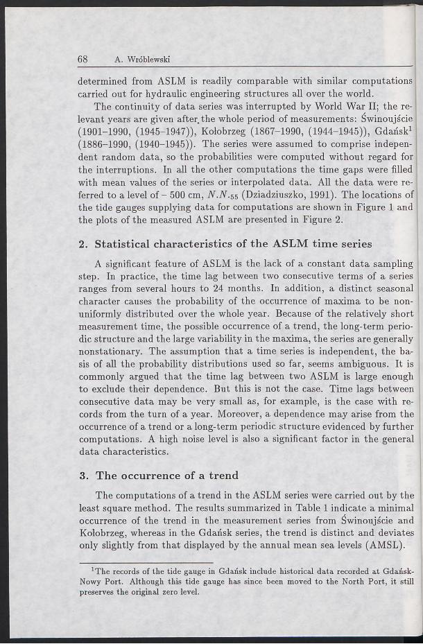
R ( k ) for a step k exceeding a certain quantity q, beyond which the au­tocorrelation is considered to have faded completely. Assuming q = 0,i.e. in the case o f a random series, var[R(k)\ & 1/N. From this va­riance, the standard error o f R(k) can be computed for a random series. Hence, formula (2) can be used for approximate testing o f the series de­pendence. In the cases analysed, the dependence should be determined from the nonstationary autocorrelation function i ? ^ ( i , i — 1). The com ­putation results for the series analysed are shown in Figure 5. The test employed is is only approximate: a definitive opinion as to the depen­dence o f the series from Świnoujście and Kołobrzeg cannot therefore be formed. It can only be stated that for those series, dependence can be sig­nificant. The independence o f the series R ^ ( t , t — 1) computed for Gdańsk on the basis o f data with a trend seems to have been proved. Clearly, the dependence o f the series from Świnoujście and Kołobrzeg may only be due to the periodic structure. For additional verification, another Bartlett’s test was applied and involved computing the cumulative periodogram (B ox and Jenkins, 1974). This test is particularly useful in revealing periodic devia­tions from randomness. A cumulative spectrum is given by the formula

Fig. 5. Computations of Barlett’s independence test, — l j for Swinoujs'cie,Kołobrzeg and Gdansk series (a), cumulative periodogram for Świnoujście series (b), cumulative periodogram for Kołobrzeg series (c)

L ( f ) = \ 5 l(g)dg, (2)Jo

whereL ( f ) - cumulative spectrum for frequency / ,Ks) ~ spectral components.When estimating power spectra by periodogram values and using a nor­malization procedure one can obtain a normalized cumulative periodogram C ( f i ) as a measure o f randomness. In the next step, deviations o f the cumu­lative periodogram from white noise values can be evaluated by employing the Kolm ogorov-Sm irnov test at an assumed significance level o f a = 0.25. It can be inferred from the computations presented in Figure 5 that as the dependence is at the limit o f statistical significance at Świnoujście it is appa­rent at Kołobrzeg. The computations carried out for Gdansk confirmed the independence o f the data. The tests applied indicate that the dependence occurring in two o f the three series studied is weak.

5. Seasonal character

The seasonal occurrence o f ASLM in the Baltic Sea area under consid­eration is primarily related to strong winds. Although this problem has been analysed in detail for Gdańsk, the conclusions drawn apply to the rest o f the measurement series. The seasonal distribution o f ASLM in Gdańsk is shown in Table 2 where the fractional powers o f ASLM occurrence were introduced wherever the maxima were repeated during the year. These data show that 74% of the ASLM were recorded during four months: No­vember, December, January and February. Only in these months are levels o f an exceeding probability p < 10% encountered. 91% o f ASLM o f with p < 25% occur during this period; the remaining 9% occur in March and October. The seasonal ASLM frequency in Gdańsk has been correlated with the occurrence o f storms in the Baltic starting from the 14th century, with the frequency o f high and low sea level deviations from the mean value, and with the occurrence o f winds o f Beaufort force 5 -7 and stronger. A similar, but not identical, seasonal ASLM distribution was noted in Great Britain (Graff, 1981).

The demonstrated seasonal nature o f ASLM linked to a 99-year obser­vation period practically excludes the occurrence o f high storm surges in months other than the four named. The large m ajority o f storm surge probability computations in oceanography are based on ASLM . When searching for alternative assumptions it seems worth taking all the mar­ked storm surges into account. A disadvantage o f such an approach is that the level from which the storm surges can be considered marked is not

Table 2. Seasonal occurrence o f annual sea level m axim a in Gdansk (1886-1939, 1946-1990). Trend eliminated; number o f data n = 99

J F M A M J J A S 0 N D TotalP < 10% n 6 2 3 5 16h > 608 % 38 13 19 30 100P < 25% n 8 3 1 2 8 10 32h > 591 % 25 9 3 6 25 32 100Total n 20 14.3 2.7 4 0.3 1 2 7 8.5 17.9 21.3 99

% 20 14 3 4 1 2 7 9 18 22 100

known. Applied to the series analysed, this assumption limits com puta­tions o f high levels to data from only four or six months in the year. This means that a seasonal probability distribution is sufficient to represent high storm surges. Empirical data o f the seasonal ASLM distribution also lead to other conclusions. It may frequently happen that ASLM observations are not carried out continuously during the year. The recording o f a ma­ximum level with a probability o f p < 10 % during the four named months permits the value obtained to be treated as the ASLM . M oreover, it seems reasonable to use water years in oceanography, as in river hydrology. The existing division into calendar years creates a dubious situation when one high storm surge occurring at the turn o f a year is recorded as tw o separate ASLM . Since water years do not divide the four-month storm period into two separate periods, they record the natural variability o f the phenomenon more faithfully.

6. Probability computations

At the beginning, comparative computations employed the generalized extreme value and Pearson’s type III distribution. The probability density function in the latter distribution is given by

f(h) = “ £)A_1; h - £’ (3)

where£ - the lower distribution limit, a,f3 -param eters, h - maximum levels.The distribution parameters were estimated by the m ethod o f moments and by the maximum likelihood method with the estimation o f the lower distri­bution limit (Kaczmarek, 1970). In Poland the Pearson type III distribution is recommended for probability computations in river hydrology.

The generalized Jenkinson distribution o f extremes (1955) is a com pre­hensive formula incorporating three distributions o f extremes derived by Fisher and Tippett (1928). The Jenkinson distribution is expressed by

h = a ( l - e~ky), (4)

wherea, k - distribution parameters, y = y{h) .Equation (4) represents three types o f curves whose slope (dy/dh) is given by the ratio o f the standard deviations o f series h and the biannual maxima o f this series, in accordance with the relation a\/o-i — 2k. It was proved that k — 0 for all the series dealt with, in which case the relationship y = y(h) is represented by a straight line. This is in accordance with the Fisher- Tippett type II distribution, worked out by Gumbel (1958) for application in hydrology

2/ = ( 1/ /5 ) (^ — M), (5 )

wherefi - 0.78<ra<Ti - standard deviation o f the series h, fi - modal value o f the series h.The probability density functions in Gum bel’s distribution are

f ( y ) = e - y - e~ y · (6)

M ethods o f estimating Gum bel’s distribution parameters have been pro­posed by many authors. Here, the maximum likelihood m ethod, worked out by Kimball (1949) and introduced to Polish hydrology by Kaczmarek (1960), was used. In this case, the relation y = a (h — fi) was considered, parameters a and // being estimated by the use o f the formulae

1 _ e-o(fc-M) = 0. (7)

1 — oc{h — n) + a(h — iJ,)e~a(h~p) = 0. (8)This method is simple as regards the computations and involves two pa­rameters only. These computations have proved the usefulness o f this ap­proach. The empirical probability was computed by the use o f the formula p = (2r — l ) / 2 N , where r denotes the current data index.

All the distributions computed were verified by x,2 test. In moment method this test was only approximate in view o f the limitations to its application. The results did not lead to the rejection o f any o f the distribu­tions. There is insufficient foundation for taking into account such factors as climatic variations and other significant parameters in forecasting future extreme sea levels. It is therefore inevitable that the fit o f the theoretical curve with respect to measurement data is decisive in the choice o f distribu­tion. The agreement between the assumed and the empirical distributions

was verified by computing the rms error in the measurement data vs. the theoretical results. The errors were small for all the distributions dealt with. Considering this test and the general advantages o f the m ethod, G um bel’s distribution was selected as the most suitable. This distribution is very common in oceanographic applications. The probability computations are summarized in Table 3. Table 4 gives the confidence intervals o f the ASLM quantiles. Figures 6, 7 and 8 show the plots o f the computations.

Table 3. Probability o f ASLM occurrence at Swinoujs'cie, K ołobrzeg and Gdańsk com puted by G um bel’s m ethod (trend elim inated)

p (% ) 99 90 80 70 60 50 40 30

T (years) 1.01 1.11 1.25 1.43 1.61 2.0 2.50 3.33Świnoujście [cm] 548 561 568 573 579 584 590 597Kołobrzeg [cm] 540 556 564 571 577 583 590 598Gdańsk [cm] 538 551 558 563 568 573 579 585P {%) 20 10 5 2 1 0.5 0.2 0.1T (years) 5.0 10 20 50 100 200 500 1000Świnoujście [cm] 605 620 633 652 665 678 695 708Kołobrzeg [cm] 609 626 642 664 680 696 717 733Gdańsk [cm] 594 608 621 639 651 664 681 694

Table 4. ASLM confidence interval limits at Swinoujs'cie, K ołobrzeg and Gdańsk for Pa = 0.683

P % 10 5 2 1 0.5 0.2 0.1Świnoujście [cm] 5 6 8 8 9 11 12Kołobrzeg [cm] 5 6 8 8 9 10 12Gdańsk [cm] 4 5 6 7 8 9 11

The probabilities were computed after the trend from the measurement series had been eliminated by the application o f the least square m ethod to the linear trend determined from the AM SL series. Such an assumption is justified by the substantial noise level in sea level maxima measurements and by the difficulties in distinguishing between the trend in ASLM forcing and that in AM SL. The increase in ASLM (either explicit or hidden by noise) is assumed to result entirely from the mean sea level rise and the vertical movements o f the Earth’s crust in the region. The uncertainty originating from such assumptions are obvious; this has also been noted in the literature

Fig. 6. ASLM probability distribution at Swinoujs'cie (trend removed) computed by Gumbel’s method

Fig. 7. ASLM probability distribution at Kołobrzeg (trend removed) computed by Gumbel’s method

Fig. 8. ASLM probability distribution at Gdańsk (trend removed) computed by Gumbel’s method

(Walden and Prescott, 1983). Mention should be made o f the fact that both the elimination o f the trend and the probability computations were referred to the first data element in the measurement series (see Tab. 1), which all terminated in 1990. In view o f the number o f data in the series the probability distributions obtained should not vary as a result o f introducing a small number o f ASLM from later measurements. A variability o f this kind may only be linked with short measurement series.

After the trend has been eliminated from the measurement series, the probability computations necessitate the inclusion o f the procedure linking this phenomenon with ASLM forecasting. The future ASLM rise is assumed to be due only to a mean sea level rise, whereas the probability distributions given in Table 3 remain unchanged. Such an assumption,' also encountered in the literature (Bardsley et al., 1990; Suthons, 1963), has been formula­ted out o f strict necessity. As for the future, three risk factors are invo­lved in forecasting ASLM probability. Firstly, changes in the probability distribution: these can be avoided by introducing a sufficient risk factor. For example, p = 0.1% can be assumed for provisional hydraulic engineer­ing structures, but p = 0.015% for first class structures (Jednoral, 1983). Additional protection will be afforded by assuming proper confidence inter­vals for the individual distribution quantiles. Secondly, taking account o f mean sea level changes is an extremely complex problem, necessitating the introduction o f certain simplifications. The rise effect in the mean water level may be regarded as due mainly to climatic forcing (e.g. the green­house effect or natural climatic recovery from the Ice Age) and many other phenomena (see NRC, 1990). Thirdly, there is the apparent effect o f sea level changes linked to vertical movements o f the Earth’s crust. The ac-

tual sea level rise (or fall) relative to the sea shore is a resultant pheno­menon. W here only the influence o f sea level changes upon the coastline is considered, the difference between these last two elements o f the risk is virtually insignificant. Forecasting the superimposition o f these two com ­ponents with a long lead time requires historical data to be taken into account. This will enable a trend equation to be formulated and hence, a forecast to be worked out. The acceleration in sea level changes also ne­eds to be examined. Protection can be afforded by introducing into the formulae a term representing the probability errors o f the prognostic trend extrapolation.

The forecast lead time o f the resultant changes in the mean sea level is not comparable with the ASLM return period. The assumed ASLM risk factor is linked with high storm sea levels against which coastlines or hydraulic engineering structures are protected. For example, a storm with a 0.1% exceedance probability may occur practically every year during the lifetime o f a hydraulic engineering structure. On the other hand, a forecast o f the resultant mean sea level rise should take account o f the forecast lead time Tl related only to the depreciation or the predicted lifetime o f the structure. For a large lead time, such a forecast is highly uncertain in view o f the problems in evaluating future vertical movements o f the Earth’s crust and in predicting all phenomena causing long-term sea level changes.

An example o f forecasting resultant AM SL can be formulated as follows. Let us assume that the resultant mean sea level rise is represented by a m onotonic trend and that there is no acceleration o f the sea level changes. It is our objective to work out a forecast with a forecast lead time Tl on the basis o f a time series o f n observations commenced in the year t . Assume also that the risk factor (see Table 3) provides sufficient protection. The error in the forecast equation must be taken into account; it is a combination o f errors in the evaluation o f quantiles o f the probability distribution, as well as the error in trend extrapolation. If the effect o f the vertical movements o f the Earth’s crust can be removed, the sea level rise for time Tl (including high probability forecast errors) should be within the limits published by a competent authority for the global estimation o f the phenomenon. The resultant formulae are

h r p = hp + a 0( t ,n ) + a i ( t , n ) T L ± e. (9)

£ = y/hl' + v2,, (10)wherehxp - sea level at time Tl with exceedance probability p,

Tl = n + 1, n + 2, n + · · ·, hp - sea level for probability p according to Table 3,

ao( t ,n ) , a i ( i , n) -regression parameters,£ - error o f the hpx estimation,hpe - error in determining quantile hp at the e probability

level,crs — error in computing the trend forecast at the s proba­

bility level,Tl - predicted depreciation or lifetime o f the structure.

The working out o f a long-term AM SL forecast for the Polish coast will be dealt with in the next part o f the study.

7. Conclusions

This paper is the first part o f a study dealing with the analysis and forecasting o f sea levels along the Polish coast. The computations followed a characterization o f the statistical features o f ASLM . All the characteristics investigated are strongly dependent on the geographical locations o f gauge stations, the number o f data and the first year o f measurements. Their nonstationary nature is revealed in the analysis o f the statistical significance o f trends, in the periodic structure, and in tests o f maxima randomness.

The investigation o f the periodic character in the oscillations o f maxima revealed certain peaks known from general sea level characteristics. A faint but nevertheless statistically marked dependence was found in the assumed random variable series from Świnoujście and Kołobrzeg. The series from Gdańsk was random.

The seasonal nature o f the data indicates that the months with the high­est storm frequency, i.e. November, December, January and February, make up a period beyond which levels with a probability exceedance less than 10% do not occur. It seems that in view o f the proven seasonal character and its consequences for the independence and representation o f annual maxima, the introduction o f water years as the data measurement period is reasonable.

The ASLM probabilities were computed by the maximum likelihood method using Gum bel’s distribution; earlier, the practicability o f Pearson’s type III distribution had been tested. The computations were carried out after the trend determined on the basis o f annual mean sea level rise had been eliminated.

In general it should be emphasized that great caution is called for when applying to oceanography the extreme value probability distributions used in river hydrology. This is mainly because o f the trend and periodic struc­ture o f the data. Any trend can be easily removed. A significant periodic structure o f the annual sea level maxima can mean that probability distri­butions formulated for random series yield dubious results.

References

Bardsley W . E., M itchell W . M ., Lennon G. W ., 1990, Estimating fu ture sea level extrem es under conditions o f sea level rise, Coastal Eng., 14, 295-303.

Bendat J. S., Piersol A . G ., 1986, Random data analysis and m easurem ent procedures, W iley-Interscience Publication, 566 pp.

B ox G. E. P., Jenkins G. M ., 1976, Tim e series analysis forecasting and control, Holden-Day Inc., 575 pp.

Chen W . Y ., Stegen G. R ., 1974, Experim ents with maximum entropy pow er spectra o f sinusoids. J. G eoph. Res., 79, 3019-3022.

Currie R. G ., 1976, The spectrum o f sea level from J, to 1,0 years, G eophys. J. R. Astron. Soc., 46, 513-520.

Das P. K ., Radhakrishna M ., 1991, An analysis o f Indian tide-gauge records, Proc. Indian A cad. S ci., 100, 177-194.

Dziadziuszko Z ., 1991, Annual mean and maximum sea levels at Polish ports, Institute o f M eteorology and W ater M anagement. M aritim e Branch, G dynia, (typescript in Polish).

Dziadziuszko Z., Jednoral T ., 1988, Variations o f sea level at the Polish Baltic Coast, Stud. Mater. Oceanol., 52, 215-238, (in Polish).

Epstein B., Lom nitz C ., 1966, A model fo r the occurrence o f large earthquakes, Nature, 211, 954-956.

Fisher R. A ., T ippett L. H. C ., 1928, Limiting form s o f the frequency distribution o f the largest or smallest m em ber o f a sample, Proc. C am b. Phil. Soc. 24, 180-190.

Germ an W . H., Levikov S. P., 1988, Veroyatnostnyj analiz i modelirovaniye kolebanii urovnya morya, Izd. G idrom eteoizdat, 181 pp.

G raff J., 1981, A n investigation o f the frequency distributions o f annual sea level maxima at ports around Great Britain, Estuarine Coastal Shelf Sci., 12, 389 - 449.

G um bel E. J., 1958, Statistics o f extrem es, C olum bia University Press, New York, 375 pp.

Jednoral T ., 1983, Application o f mathematical statistics to sea researches, M aritim e Institute, Gdańsk, 207 pp., (in Polish).

Jenkinson A . F., 1955, The frequency distribution o f the annual maximum (o r minim um ) values o f meteorological elem ents, Quart. J. Roy. M et. Soc., 81, 158-171.

Kaczm arek Z., 1960, Confidence interval as measure o f accuracy o f the probable flood estimation, W iad. S. Hydrol. M eteorol., 7, 133-185, (in Polish).

Kaczm arek Z., 1970, Statistic methods in hydrology and m eteorology, PIHM , 311 pp., (in Polish).

K im ball B. F., 1949, A n approximation to the sampling variance o f an estimated maximum value o f given frequency based on fit o f double exponential distribution o f maximum values, Ann. M ath. Stat., 20, 110-113.

Kowalik Z., Wróblewski A., 1973, Long-term oscillations o f annual mean sea levels in the Baltic on the basis o f observations carried out in Świnoujście from 1811 to 1970, Acta Geoph. Pol., XXI, 3-10.

Mazzarella A., Palumbo A., 1991, E ffect o f sea level tim e variations on the occurrence o f extrem e storm -surges: an application to the N orthern Adriatic Sea, Boll. Oceanol. Teor. appl., IX, 33-38.

Monin A. S., Vulis I. L., 1971, On the spectra o f long-period oscillations o f geophysical param eters, Tellus, 23, 337-345.

NRC (US), 1990, Sea level changes, National Academy Press, Washington D.C., 234 pp.

Pickands III, J., 1975, Statistical in ference using extrem e order statistics, Ann. Statistics 3, 119-131.

Pugh D. T., Vassie J. M., 1980, Applications o f the jo in t probability method fo r extrem e sea level computations, Proc. Inst. Civ. Eng., 9, 361-372.

Strupczewski W., 1967, D eterm ination o f the probable annual distribution o f som e events on basis o f all their occurrences, Acta Geoph. Pol., XV, 247-262.

Suthons C. T., 1963, Frequency o f occurrence o f abnormally high sea levels on the east and south coast o f England, Proc. Inst. Civ. Eng., 25, 443-449.

Walden A. T., Prescott P., 1983, Identification o f trends in annual maximum sea levels using robust locally weighted regression, Estuarine Coastal Shelf Sci., 16, 17-26.

Wróblewski A., 1974, Spectral densities o f long-period oscillations in the levels o f the Baltic Sea, Oceanologia, 3, 33-50, (in Polish).