PPA 723: Managerial Economics Lecture 9: Applications of Consumer Choice.

PPA 723: Managerial Economics

Lecture 9:

Applications of Consumer Choice

Managerial Economics, Lecture 9: Applications of Consumer Choice

Outline

The Labor-Leisure ChoiceApplication to welfare programs

Measuring Consumer WelfareThe concept of consumer surplus


Deriving Labor Supply Curves

Use consumer-maximization diagram with income (= all goods consumed) on the vertical axis and leisure (= non-work) on the horizonal axis.

Income equals the wage times hours worked.

The wage rate is the price of leisure.

Managerial Economics:Consumer Choice

Figure 5.8 Demand for Leisure

Y, Goodsper day

Time constraint

H2 = 12 H1 = 824 0N2 = 12 N1 = 160 24

H, Work hours per dayN, Leisure hours per day

H2 = 12 H1 = 8N2 = 12 N1 = 160

H, Work hours per dayN, Leisure hours per day

Demand for leisure

I 2

I11

–w2

L1

L2

(a) Indifference Curves and Constraints

w, Wageper hour

(b) Demand Curve

–w11

e2Y2

Y1

w1

w2

e1

E2

E 1


Supply Curve of Labor

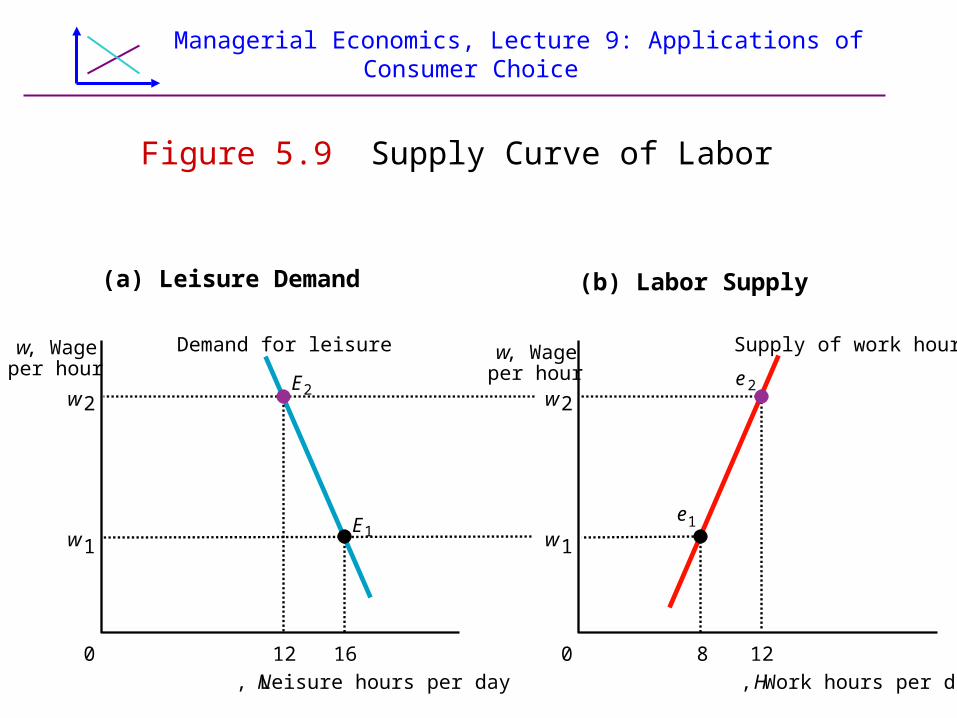
The supply curve of hours worked (labor) is the “mirror image” the of demand curve for leisure:

Every extra hour of leisure implies one fewer hours of work.


Figure 5.9 Supply Curve of Labor

w, Wageper hour

(a) Leisure Demand

Demand for leisure

w1

w2

16120

N, Leisure hours per day

E1

E2

w, Wageper hour

(b) Labor Supply

Supply of work hours

w1

w2

8 120

H, Work hours per day

e2

e1


Income and Substitution Effects

A wage increase causes both income and substitution effects that alter an individual's demand for leisure and supply of hours worked.

The substitution effect leads to more work.

The income effect leads to more leisure.


Figure 5.10 Income and Substitution Effects of a Wage ChangeY, Goods

per dayTime constraint

H 2H * H124 0

N 2N * N10 24

Substitution effect

Income effect

Total effect

H, Work hours per day

N, Leisure hours per day

I 2

I1

L 2

L*

L1

e2

e1

e*


Goods per Day, Y

Leisure Hours per Day, L Work Hours per Day

Time Constraint

0 L1

Guarantee

1

-wage

L2

Leisure Choice with a Welfare Guarantee



Time Constraint

0 L1 L2 L3

Income Effect

Substitution Effect

Slope = -w(1-t)

Guarantee

Goods per Day, Y

Leisure Choice with a Welfare Guarantee and “Tax” Rate



Time Constraint

0 L1 L2L3

Income Effect

Substitution Effect

Slope = -w(1+e)

Goods per Day, Y

Leisure Choice with an EITC


Gross Income vs. Earned IncomeSource: Clifford F. Thies on the mises.org blog.


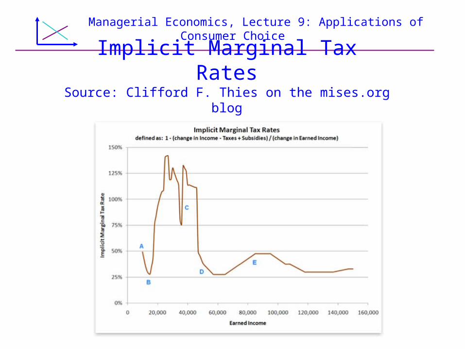
Implicit Marginal Tax RatesSource: Clifford F. Thies on the mises.org blog


Welfare Programs: Lessons

Income guarantees raise recipients’ utility but decrease their work effort.

Income guarantees with benefit reduction rates decrease work effort even more.

Training programs, child care credits, and the EITC raise utility while boosting work effort.


Consumers’ WelfareMeasuring welfare with utility functions

is not practical for 2 reasons:we don't know individuals' utility functionswe cannot compare utilities across

individuals

Instead, we measure consumer welfare in dollars of willingness to payeasier to measure than utilitycan compare dollars across individuals


Measuring Consumer Welfare Consumer surplus (CS) from a good =

benefit a consumer gets from consuming it (in $'s) minus its price

how much more you'd be willing to pay than you did pay for a good

A demand curve contains this information.

A demand curve reflects a consumer's marginal benefit= the amount a consumer is willing to pay for an extra unit.


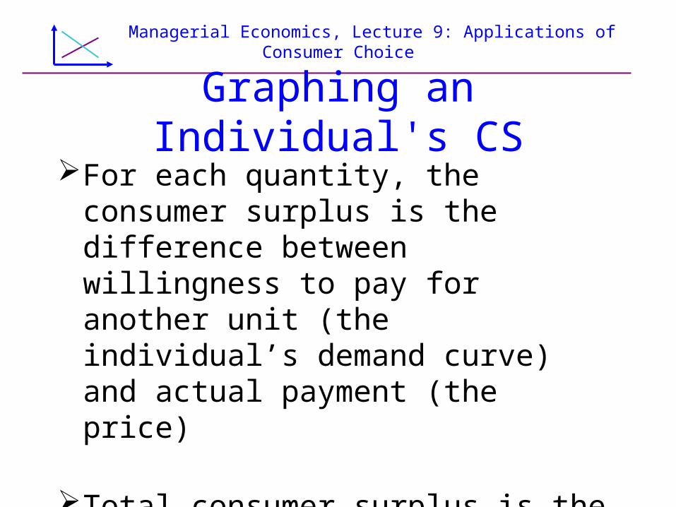
Graphing an Individual's CSFor each quantity, the consumer surplus

is the difference between willingness to pay for another unit (the individual’s demand curve) and actual payment (the price)

Total consumer surplus is the sum of these differences across all quantities consumed.


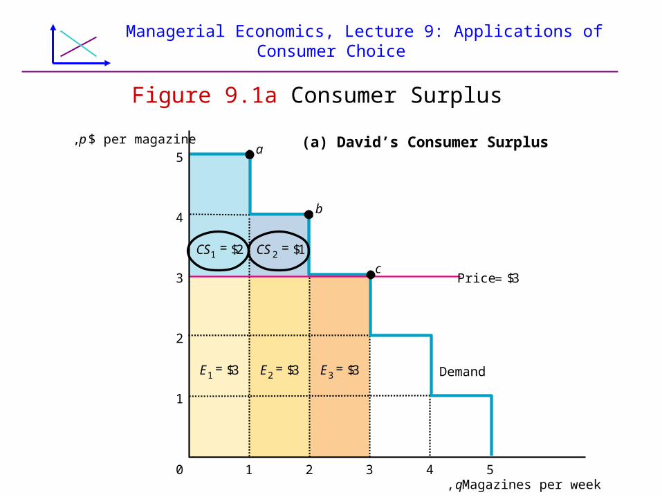
Figure 9.1a Consumer Surplus

5

4

3

2

1

543210

CS2 = $1CS1 = $2

E1 = $3 E2 = $3 E3 = $3

Price = $3

a

b

c

q, Magazines per week

p, $ per magazine (a) David’s Consumer Surplus

Demand


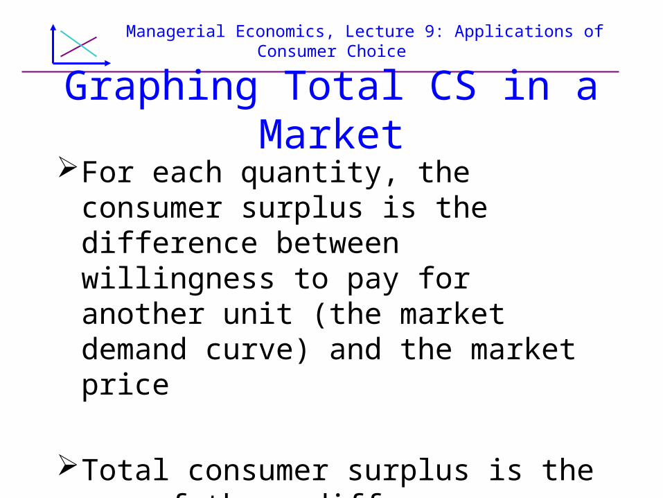
Graphing Total CS in a MarketFor each quantity, the consumer surplus

is the difference between willingness to pay for another unit (the market demand curve) and the market price

Total consumer surplus is the sum of these differences across all quantities consumed.


Figure 9.1b Consumer Surplus

p 1

p, $ pertrading card

q1 q, Trading cards per year

DemandExpenditure, E

Consumersurplus, CS

Marginal willingness topay for the last unit of output

’


Concluding Comment on CS

As we will see, consumer surplus is a key concept in policy economics.

It forms the basis for benefit-cost analysis.

CS is used to determine whether a policy is efficient and to measure the distortion in behavior caused by a tax.


Producer Surplus

Suppliers’ gain from participating in a market, too.

Their surplus is the difference between the amount for which a good sells and minimum amount necessary for the seller to produce that good.


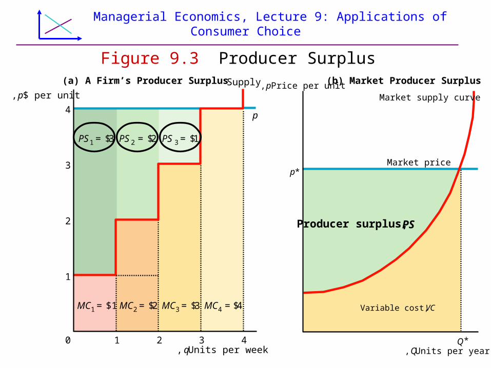
Measuring PS Using the Supply Curve

Producer surplus for a competitive firm or market is:

the area above supply curve (which, as we will later learn, is the MC curve) and below price line up to quantity sold


4

3

2

1

43210

PS2 = $2 PS3 = $1PS1 = $3

MC2 = $2 MC3 = $3 MC4 = $4MC1 = $1

p

Supply

q, Units per week

p, $ per unit

(a) A Firm’s Producer Surplus

p*

p , Price per unit

Q*

Market supply curve

Q, Units per year

Market price

Variable cost, VC

Producer surplus, PS

(b) Market Producer Surplus

Figure 9.3 Producer Surplus


Producer Surplus and Social Welfare

Some analysts define social welfare as consumer surplus plus producer surplus.

Others focus exclusively on consumer surplus.

This is an issue in normative analysis, that is, it involves value judgments.

Date post:	26-Dec-2015
Category:	Documents
Upload:	aron-carr
View:	215 times
Download:	3 times

PPA 723: Managerial Economics Lecture 9: Applications of Consumer Choice.

Documents