PERIODIC TRAVELING WAVES GENERATED BY INVASION INCYCLIC PREDATOR–PREY SYSTEMS: THE EFFECT OF
UNEQUAL DISPERSAL∗
JAMIE J. R. BENNETT† AND JONATHAN A. SHERRATT†
Abstract. Periodic traveling waves (wavetrains) have been an invaluable tool in the understand-ing of spatiotemporal oscillations observed in ecological data sets. Various mechanisms are knownto trigger this behavior, but here we focus on invasion, resulting in a predator–prey-type interaction.Previous work has focused on the normal form reduction of PDE models to the well-understood λ-ωequations near a Hopf bifurcation, though this is valid only when assuming an equal rate of dispersionfor both predators and prey—an unrealistic assumption for many ecosystems. By relaxing this con-straint, we obtain the complex Ginzburg–Landau normal form equation, which has a one-parameterfamily of periodic traveling wave solutions, parametrized by the amplitude. We derive a formulafor the wave amplitude selected by invasion before investigating the stability of the solutions. Thisgives us a complete description of small-amplitude periodic traveling waves in the governing modelecosystem.
1. Introduction. It is well known that populations can cycle under certain eco-logical conditions, meaning there are temporal oscillations in abundance. Mathemati-cal modeling has provided insight into the mechanisms that drive cyclic behavior [41],though the spatial nature of the process is less well understood. In some cases, cyclicpopulations oscillate uniformly across their habitat, but spatiotemporal patterningis also well documented [1, 17, 40] and has been known to severely disrupt someecosystems. As an example, North America has an ongoing problem with spatiallyheterogeneous cyclic mountain pine beetle outbreaks that spread through and destroyvast areas of woodland. In the Rocky Mountain region of British Columbia alone,approximately 17 million acres of forest were infested by mountain pine beetles in2004 compared to 0.4 million in 1999 [45], with impacts ranging from fire hazards tochanges in the carbon cycle [12].
One important type of spatiotemporal patterning is periodic traveling waves(PTWs); peaks in population density move across the domain with constant shapeand speed. In field data, such a pattern might manifest itself via peak and troughpopulation densities being observed simultaneously at different locations—the two lo-cations would appear to oscillate out of phase. Spatiotemporal data is difficult andcostly to obtain, but there are a number of data sets that provide evidence of peri-odic traveling wave phenomena [17, 26, 38]. For instance, data has been collected on
∗Received by the editors December 8, 2016; accepted for publication (in revised form) June 28,2017; published electronically November 30, 2017.
http://www.siam.org/journals/siap/77-6/M110718.htmlFunding: The first author’s work was supported by The Maxwell Institute Graduate School in
Analysis and Its Applications, a Centre for Doctoral Training funded by the UK Engineering andPhysical Sciences Research Council (grant EP/L016508/01), the Scottish Funding Council, Heriot-Watt University, and the University of Edinburgh.†Department of Mathematics and Maxwell Institute for Mathematical Sciences, Heriot-Watt
PERIODIC TRAVELING WAVES IN PREDATOR–PREY SYSTEMS 2137
larch budmoth populations demonstrating that waves in budmoth population densitypropagate across the Swiss Alps at an estimated speed of 210 km per year toward thenortheast [4]. To be clear, these waves are not a result of individuals migrating acrossthe landscape at 210 km per year but are a consequence of the governing cyclic natureof the budmoth’s overall population, coupled with an intrinsic spatial dependence ofthe individuals. The same phenomenon is observed in oscillatory chemical reactionssuch as the BelousovZhabotinsky reaction [9].
The mathematical theory of PTWs has been instrumental in the understanding ofwaves observed in cyclic populations. A PTW is defined mathematically as a periodicfunction of both (one-dimensional) space and time. We model our populations using aset of partial differential equations; spatial terms are added to a set of coupled ordinarydifferential equations with a (stable) limit cycle. If a PTW solution exists for a givenmodel, general theory implies that there exists a family of possible solutions [25], ofwhich one is selected by imposed initial and boundary conditions that correspond toa particular ecological situation. This means one can know all parameter values in amodel but be unable to predict the characteristics of PTWs seen in practice. It is,therefore, instructive to focus both on one specific type of ecological interaction andone pattern-generating scenario relevant to that interaction.
In this paper, we focus on predator–prey interactions. There are a number ofecological situations one could consider in a predator–prey system that would generatePTWs, including heterogeneous habitats [4, 13], hostile boundaries [31], migrationdriven by pursuit and evasion [3], and an invasion of alien species [23]. In this paper,we consider the latter of these mechanisms. Geographic features such as oceans,mountains, and forests prevent the interaction of species in different locations. Naturalevents can cause these divides to be bypassed, but humans especially are responsiblefor the introduction of foreign species today [7, 39]. Understanding invasions and thebehavior left in their wake is therefore of considerable practical importance.
We model the predator–prey interaction in one space dimension using a reaction–diffusion system. Let Y(x, t) ∈ R2 represent predator and prey population densitiesdependent on space, x, and time, t. A general two-species predator–prey system canbe written as
(1)∂Y∂t
= F(Y;µ) + D∂2Y∂x2 ,
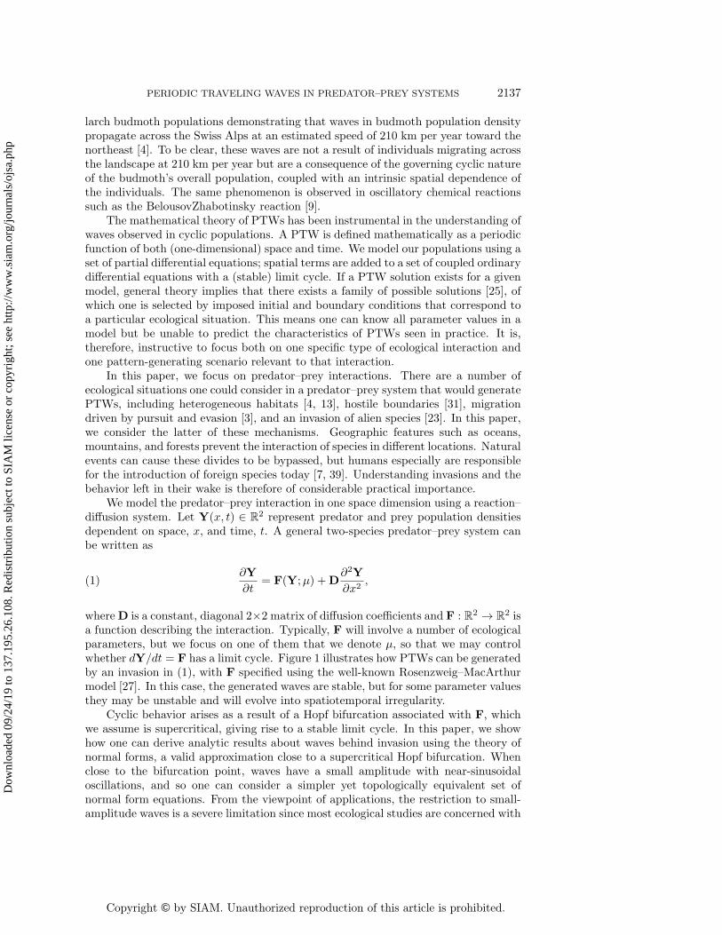
where D is a constant, diagonal 2×2 matrix of diffusion coefficients and F : R2 → R2 isa function describing the interaction. Typically, F will involve a number of ecologicalparameters, but we focus on one of them that we denote µ, so that we may controlwhether dY/dt = F has a limit cycle. Figure 1 illustrates how PTWs can be generatedby an invasion in (1), with F specified using the well-known Rosenzweig–MacArthurmodel [27]. In this case, the generated waves are stable, but for some parameter valuesthey may be unstable and will evolve into spatiotemporal irregularity.
Cyclic behavior arises as a result of a Hopf bifurcation associated with F, whichwe assume is supercritical, giving rise to a stable limit cycle. In this paper, we showhow one can derive analytic results about waves behind invasion using the theory ofnormal forms, a valid approximation close to a supercritical Hopf bifurcation. Whenclose to the bifurcation point, waves have a small amplitude with near-sinusoidaloscillations, and so one can consider a simpler yet topologically equivalent set ofnormal form equations. From the viewpoint of applications, the restriction to small-amplitude waves is a severe limitation since most ecological studies are concerned with
Fig. 1. An illustration of invasion of predators into prey for cyclic populations. Numericalsolutions of (18) are plotted as functions of space, x, at successive times, t. The vertical separationbetween plots is proportional to the time interval, with time increasing up the plot. Advancingand receding wave fronts of predator and prey, respectively, move from left to right, behind whichis a band of periodic traveling waves. Parameter values are A = 2, B = 3, C = 5, δ = 1; initialconditions correspond to a prey-only state everywhere except for a small perturbation at the left-handboundary.
large amplitude cycles. However, the generation of large-amplitude periodic travelingwaves remains an open problem mathematically, and the study of small-amplitudewaves provides an important framework for the interpretation of simulation-basedstudies of the larger-amplitude case. Previous work on small-amplitude cycles hasfocused on the special case where D = I, for which the normal form can be written as
(2)∂u
∂t= (1− r2)u+ αr2v +
∂2u
∂x2 ,∂v
∂t= (1− r2)v − αr2u+
∂2v
∂x2 ,
with r2 = u2 + v2, an equation of λ-ω type first described by Kopell and Howard [14].α is an expression containing the original model parameters in (1) and is determinedvia a normal form calculation that we will describe in section 2. Kopell and Howardshowed that (2) have a one-parameter family of PTW solutions of the form
(3) u = r0 cos(±√
1− r20x− αr2
0t
), v = r0 sin
(±√
1− r20x− αr2
0t
),
for all r0 such that 0 ≤ r0 ≤ 1. Furthermore, they showed that the generated wavesare linearly stable as a solution of (2) if and only if
(4) 2(1− r20)(1 + α2)− r2
0 ≤ 0.
Sherratt [29] derived an amplitude formula for PTWs generated by invasion in theλ-ω equations,
PERIODIC TRAVELING WAVES IN PREDATOR–PREY SYSTEMS 2139
which, together with (3) and (4), give a complete description of low-amplitude wavesgenerated by invasion in a predator–prey model given by (1) with D = I.
In section 2, we review the theory of normal forms, showing that the normal formof (1) for general D is the cubic complex Ginzburg–Landau equation, giving explicitformulae for its coefficients. One way of obtaining the λ-ω normal form equationsis to have D = I, implying that predator and prey dispersal rates are equal (anunrealistic assumption in many ecosystems). We prove the existence of alternativemodel constraints for a normal form reduction of λ-ω type in section 3, allowing oneto study the effects of unequal dispersal using the established theory detailed in thissection. The most general case is considered thereafter; in particular, a formula for thewave amplitude is derived for PTWs generated by invasion in the complex Ginzburg–Landau equations in section 4, allowing us to draw conclusions about stability insections 5 and 6. This work allows us to study small-amplitude PTWs for general Fand D, i.e., for any model in the form (1). In section 7, we illustrate our results viaan example.
2. Normal form coefficients: A review. There is a large, well-establishedvolume of work that involves reducing (1) in the absence of diffusion to a topologicallyequivalent “normal” form under the assumption of small-amplitude limit cycles [10,16]. This corresponds to being close to a Hopf bifurcation parameter in order to obtainnear-sinusoidal oscillations. We consider solutions of (1) that are close in parameterspace to this homogeneous oscillatory solution. Kuramoto [15] uses a method ofmultiple scales applied to space and time variables in order to reduce (1) to normalform. The Stuart–Landau equations are first derived for the homogeneous solutionbefore results are extended to include diffusion terms. We give a brief review of thecalculation, but a complete and detailed treatment can be found in Kuramoto’s book.
Let us assume that Y0(µ) is a homogeneous steady state of (1) so that F(Y0(µ);µ)= 0. One can express (1) in terms of u = Y −Y0 as a Taylor series expansion,
(6)∂u∂t
=(
J + D∂2
∂x2
)u + Muu + Nuuu + . . . ,
where J is the standard Jacobian matrix evaluated at Y0. Muu and Nuuu denotequadratic and cubic terms in u, respectively, where the ith element is given by
(7) (Muu)i =12!
∑j,k
∂2Fi∂Yj∂Yk
∣∣∣∣Y0
ujuk, (Nuuu)i =13!
∑j,k,l
∂3Fi∂Yj∂Yk∂Yl
∣∣∣∣Y0
ujukul.
M is sometimes referred to as the Hessian matrix. We denote elements of vectorsusing subscripts so that, for example, Fi is the ith element of F. The stability of Y0
for space-independent perturbations is determined by the eigenvalues associated withJ. We let λ(µ) = σ(µ) + iω(µ) denote an eigenvalue that is becoming critical withcomplex conjugate, λ(µ), and beyond the critical parameter value, µcrit, the steadystate, Y0, becomes unstable, generating a limit cycle in the homogeneous system.For the nonhomogeneous case, we assume the same—that instability is a result of acomplex conjugate pair of eigenvalues associated with J becoming purely imaginary atµcrit. In assuming this, we are neglecting the possibility of diffusion-driven instability,i.e., Turing patterns.
where ε2χ = (µ − µcrit), χ = sgn(µ − µcrit), and λν = σν + iων . χ is introducedhere because we have not yet specified whether a limit cycle is generated for µ < µcritor µ > µcrit, and so we ensure that ε is always well defined. The quantities J0,M0, and N0 are the matrices J, M, and N, respectively, evaluated at µcrit. Ourassumptions imply that σ0 = 0 in order to ensure that eigenvalues associated withthe homogeneous linearized problem are purely imaginary when µ = µcrit. Let U andU∗ be right and left eigenvectors, respectively, associated with J0 and the eigenvalueλ0. Then λ0 = iω0 = U∗J0U and
(9) λ1 = σ1 + iω1 = U∗J1U.
We have used the fact that the eigenvectors are normalized such that U∗U = U∗U =1, where a bar denotes a complex conjugate. Also, note the standard relationshipU∗U = U∗U = 0.
The eigenvalue λ has a small real part of order ε2, and so we introduce a scaledtime variable defined by τ = ε2t. A slow space dependence is also anticipated dueto the slow spatiotemporal dynamics close to the Hopf bifurcation point, and so wewrite u = u(t, τ, s), scaling space as s = εx. It can then be shown [15] by substitutionof (8) into (6) that Y(t, τ, s) is approximated close to the Hopf bifurcation point bythe equation
whereW (τ, s) is some complex amplitude that satisfies the unscaled complex Ginzburg–Landau equation
(10)∂W
∂τ= χλ1W − g|W |2W + d
∂2W
∂s2 ,
with d = U∗DU,(11a)and g = −2U∗M0UV0 − 2U∗M0UV+ − 3U∗N0UUU,(11b)
where V+ = −(L0 − 2iω0)−1M0UU and V0 = −2L0−1M0UU. The real and imag-
inary parts of W represent predator and prey population densities. With this result,we have outlined the calculations necessary to obtain the normal form coefficients(9) and (11), so that close to a Hopf bifurcation, one can reduce (1) to (10). Noticethat (10) has no dependence on the control parameter µ due to the scalings we havemade in space and time. We can further reduce the equation to the scaled complexGinzburg–Landau equation (CGLE)
PERIODIC TRAVELING WAVES IN PREDATOR–PREY SYSTEMS 2141
One obtains (12) by performing the change of variables:
τ → 1σ1τ , s→
√Re(d)σ1
s , W →√
σ1
|Re(g)|eiω1σ1
τW.(14)
All predator–prey models of the form (1) can be reduced to (12) with the assumptionsdetailed above, and so we can now safely focus our attention on the CGLE with theknowledge that results are related directly via (14).
In general, a predator–prey model of the form (1) gives nonzero α and β. However,in some special cases, one can obtain β = 0, and then (12) is simply the λ-ω equations(2), for which the results outlined in section 1 apply. Note that in this scenario, anydiffusion coefficients in the original model are scaled out via (14). We now considerwhat features of (1) result in β = 0 and, hence, a normal form of λ-ω type.
3. Conditions for equations of λ-ω type. Predator–prey interactions inwhich populations tend to move about their habitats at similar rates can be rep-resented in our model ecosystem by setting the dispersal coefficient of the predatorpopulation equal to that of the prey, i.e., D = I. This is appropriate for manyaquatic micro-organisms [11], but the ratio of predator to prey dispersal rates will besignificantly greater than one for most mammalian systems [5] and, also, for macro-scopic marine species [44]. When D = I, one can clearly see that (11a) collapses tod = U∗IU = 1 and implies β = 0 in (12), yielding λ-ω-type equations (2). We nowshow that D = I is sufficient but not necessary in order to obtain equations of λ-ωform, allowing one to study the effects of unequal diffusion using theory described insection 1. We prove the following theorem:
Theorem 3.1. Consider (1) and let F(Y;µ) := (F1(Y;µ), F2(Y;µ))T be suchthat populations represented by Y(x, t) := (Y1(x, t), Y2(x, t))T are cyclic as a resultof a supercritical Hopf bifurcation. A normal form reduction then yields equations ofλ-ω type if at least one of the following conditions hold:
(i) D = I,
(ii)∂F1
∂Y1
∣∣∣∣Y0,µcrit
=∂F2
∂Y2
∣∣∣∣Y0,µcrit
= 0.
Proof. For β = 0, we need Im(d) = 0. We consider equation (11a) and write U,J0, and D in terms of their components:
U :=(u1 + iv1u2 + iv2
), J0 :=
(j1 j2j3 j4
), D :=
(δ1 00 δ2
),
where u1, u2, v1, v2, j1, j2, j3, j4, δ1, δ2 ∈ R. Note that since J0 is at criticality, i.e.,µ = µcrit, we express the purely complex eigenvalues associated with J0 as
The left eigenvalue U∗ can be calculated in terms of u1, u2, v1, v2 so that (11a)implies
d =1
2(u1v2 − u2v1)
(v2 + iu2−v1 − u1
)T (δ1 00 δ2
)(u1 + iv1u2 + iv2
),
the imaginary part of which can be written as
Im(d) =12
(u1u2 + v1v2)(δ2 − δ1)(u1v2 − u2v1)
.
For Im(d) = 0, we require δ1 = δ2 (i.e., D = I), or
u1u2 + v1v2 = 0.(17)
One can easily show that the eigenvectors associated with J0 and (15) are given by
j2(u2 + iv2) =(i√j1j4 − j2j3 − j1
)(u1 + iv1) ,
j3(u1 + iv1) =(i√j1j4 − j2j3 − j4
)(u2 + iv2) .
Without loss of generality, choose u1 + iv1 = j2 and u2 + iv2 = i√j1j4 − j2j3 − j1.
Then (17) implies that j1j2 = 0. Together with (16), we have j1 = 0 and j4 = 0with either j2 < 0 and j3 > 0, or j2 > 0 and j3 < 0. Note that j2 6= 0 because (16)would not be satisfied. Recall that J0 is simply the Jacobian matrix evaluated atboth Y = Y0 and µ = µc.
We have discussed Theorem 3.1(i) and its ecological significance. We now provide anexample of a widely used predator–prey model for which Theorem 3.1(ii) applies.
Example: The Rosenzweig–MacArthur model. In order to reduce the num-ber of parameters that need to be considered, we present the well-known Rosenzweig–Macarthur model [27] in its nondimensionalized form
∂p
∂t=∂2p
∂x2︸︷︷︸dispersal
+
benefit from predation︷ ︸︸ ︷cph
b(1 + ch)− p
ab︸︷︷︸death
, predators(18a)
∂h
∂t= δ
∂2h
∂x2︸ ︷︷ ︸dispersal
+
logistic growth︷ ︸︸ ︷h(1− h)− cph
1 + ch︸ ︷︷ ︸predation
. prey(18b)
The scaled predator and prey densities p and h, respectively, are functions of space,x, and time, t. The omitted nondimensionalization means that parameters a, b, c, δcorrespond to ratios of ecological quantities. a is the ratio of predator birthrates anddeath rates, b is the ratio of prey and predator birthrates, c is the product of preycarrying capacity and a rate associated with how fast prey consumption saturatesas the number of prey increases, and δ is the ratio of prey and predator disperalcoefficients. For a full model description see, for example, [30].
PERIODIC TRAVELING WAVES IN PREDATOR–PREY SYSTEMS 2143
0 0.5 1 1.5 2 2.5
50
100
150
200
250
Fig. 2. A plot to show the relationship between the wavelength of PTWs generated in (18)with the diffusion coefficient, δ. Points and lines indicate numerical simulation and analytic ap-proximation, respectively. Parameter values are set to a = 3 and b = 4, giving a Hopf bifurcationpoint at ccrit = 2. We consider three different values of c:c = 3 (dot-dashed line and squares),c = 2.4 (dashed line and circles), and c = 2.1 (solid line and crosses)—to show the convergence ofthe analytic approximation to the numerical simulation as the Hopf bifurcation point is approached.
There exists one coexistence steady state (p, h) = (ps, hs), where hs = 1/c(a− 1)and ps = ahs(1− hs). The Jacobian at (ps, hs) is then given by
J =
0ac− c− 1
acb
−1a
ac− a− c− 1ac(a− 1)
.
One can easily see that the upper left entry is a zero because the rate of changeof predator population density is linear in p, neglecting spatial terms. Let c be ourcontrol parameter without loss of generality. At criticality, we see that the bottomright entry is forced to be zero by definition, with the critical value of the parametergiven by ccrit = (a+ 1)/(a− 1), and so we have satisfied Theorem 3.1(ii).
In a similar way, we obtain a normal form reduction of λ-ω type if, for arbitraryfunctions gp, gh : R→ R, either the predator kinetics have the form p ·gp(h) like (18a)or the prey kinetics have the form h · gh(p). In such cases, we can make predictionsabout PTWs via (3)–(5), noting the scalings made in section 2. Figure 2 illustratesthe effect of dispersal on the wavelength of PTWs. Close to the Hopf bifurcation, thetheory describes PTWs well, and analytic predictions match numerical simulationsaccordingly. Farther away, accuracy is lost as PTWs become larger and less sinusoidal.Theorem 3.1(ii) turns out to be a common feature of many predator–prey models, butthe remainder of this paper considers the more general case when (1) satisifes noneof the conditions in Theorem 3.1, with the aim of giving a comprehensive method forstudying low-amplitude PTW solutions generated by invasion.
4. Amplitude behind invasion in the CGLE. As discussed in section 2, thenormal form of (1) in general is the CGLE. Here, we return to the standard x and tnotation for the analysis of (12). The CGLE is particularly well studied in the physicscommunity due to its rich dynamics and varied applications [2]. One of the simplestpattern structures that one can generate are PTWs (sometimes called plane waves)given by
where r20 = 1− q2 > 0 and ω = (β − α)q2 + α. This family of solutions is effectively
parametrized by the amplitude of the PTW, and so in this section we aim to derive anamplitude equation corresponding to an invasion. Let us first be more precise aboutwhat we mean by an invasion. In ecological terms, we want a prey-only environmentwith a small introduction of predators near the edge of the habitat. This prey-onlyenvironment would be the unstable steady state of the predator–prey model; however,the CGLE has a zero unstable steady state obtained via a recentering in the normalform calculation. Mathematically, for some small p ∈ R, we consider initial conditionsof the form
(20a) W (x, 0) =
{p, x = 0,0, x > 0,
on a semi-infinite domain [0,∞). The physical interpretation becomes apparent whenone considers the complex counterparts that make up W ; Re(W ) and Im(W ) canbe interpreted as predator and prey equations, respectively. We specify boundaryconditions as
∂W
∂x= 0 at x = 0 and W → 0 as x→∞;(20b)
however, numerical simulations show that the left-hand boundary condition affects thebehavior of the solution only locally so that one may consider a different condition atx = 0 without affecting the generated PTWs.
To simplify analysis, we represent the complex amplitude W in terms of its realamplitude and phase,
rt = rxx − β (rθxx + 2rxθx)− rθ2x + r(1− r2)(21a)
θt = θxx + β(rxxr− θ2
x
)+
2rxθxr− αr2,(21b)
by letting r = |W | and tan(θ) = Im(W )/Re(W ). Observing numerical simulations ofr (Figure 3(a)) reveals a transition wave moving across the domain in the positive xdirection, which changes the amplitude of the solution from zero to that of the gen-erated PTW. One would not expect the same behavior when plotting θ, but previousanalysis of the CGLE, for example, [2] (and also of the λ-ω equations [14]), promptsus to consider the phase gradient ψ := θx, plotted in Figure 3(b). A transition wavein ψ can clearly be seen moving in parallel with that of r, and so we seek a travelingwave solution of the form r(x, t) = r(x − ct) and ψ(x, t) = ψ(x − ct), which impliesθ(x, t) = Ψ(x, t) + f(t), where Ψ is some indefinite integral of ψ and f is a functionto be determined. We get two second-order ordinary differential equations,
r′′ + cr′ + r − r3 − rψ2 − β(rψ′ + 2r′ψ
)= 0
ψ′ + cψ − αr2 +2r′ψr− β
(ψ2 − r′′
r
)− f ′(t) = 0,
where a prime denotes differentiation with respect to z = x − ct. We define a newparameter φ = −r′/r, following, for example, [42], in order to reduce the system tothree first-order differential equations,
PERIODIC TRAVELING WAVES IN PREDATOR–PREY SYSTEMS 2145A(x
;t)
0.3
0.4
0.5
0.6
x4000 4200 4400 4600 4800 5000
?(x
;t)
0
0.5
1
r(x;t
)
0
0.4
0.8
(a)
(b)
(c)
ψ0
φ0
Fig. 3. Typical solutions for (a) r(x, t), (b) ψ(x, t) = θx, and (c) φ(x, t) = rxx/r. We plot thesolution at equally spaced time intervals, revealing a transition wave that moves across the domainin the positive x direction. Ahead of the wave front, r → 0, ψ → ψ0, and φ → φ0; constants thatare easily determined analytically, the details of which can be found in the text. The constant valuebehind the transition front in (a), (b), and (c) corresponds to a particular PTW, selected by aninvasion given by (20). We use parameter values α = 1, β = 0.4 and plot solutions until r is ofthe order 10−15. The amplitude of periodic traveling waves generated by an invasion (behind thewave front in (a)) can be expressed in terms of parameter values as (27). This formula gives theamplitude as 0.827 to three significant figures.
where tildes have been dropped. Figure 3 illustrates how all variables tend towardconstant values, r → 0, ψ → ψ0, and φ → φ0 as x → ∞, where ψ0 and φ0 areconstants. Examining the behavior of the system for large x will give us an expressionfor f , allowing us to calculate the steady states of (22) in terms of α and β.
The quantities φ0, ψ0, and c can be derived using the theory of front propagationinto unstable steady states, for which a detailed review has been collated by van Saar-loos [43]. Equation (12) has a linearly unstable steady state at W = 0, implying thatour localized initial condition (20a) will grow and spread in the positive x-direction,as we have seen. There are two classes of traveling front that can develop: either a“pulled” front or a “pushed” front, both of which travel at different speeds in the limitt → ∞. Our initial conditions are sufficiently “steep” (see [43]) for a pulled front todevelop, and therefore c is the asymptotic linear spreading speed associated with thedynamical equations obtained by linearizing the CGLE. It is easily calculated from
the linear dispersion relation along with φ0 and ψ0. If one decomposes W into Fouriermodes, we can write
W (k, t) =∫ ∞−∞
W (x, t)e−ikxdx
and calculate the linear dispersion relation, ω(k) via the substitution of the ansatz,
W (k, t) = W (k)e−iω(k)t,(23)
giving ω(k) = (β− i)k2 + i. The inverse Fourier transform and (23) can then be usedto write
W (x, t) =1
2π
∫ ∞−∞
W (k)eikx−iω(k)tdx,(24)
where W is just the Fourier transform of the initial condition.Consider two observers initially located at x = 0 who move off in the positive
x-direction along with the wave front. The first observer is moving at some speedgreater than c and so will eventually see the unstable zero steady state that is beinginvaded, whereas the observer moving at some speed less than c will eventually seethe invasive stable steady state, which in our case takes the form of PTWs. If weconsider a moving frame of reference z = x − ct, the front should neither grow nordecay. Then (24) becomes
W (z, t) =1
2π
∫ ∞−∞
W (k)eikz−i[ω(k)−ck]tdk,
which can be evaluated using the method of steepest descent (saddle point approxi-mation) due to the large time limit. The saddle point, k∗, is given by
d[ω(k)− ck]dk
∣∣∣∣k∗
= 0 =⇒ c =dω(k)
dk
∣∣∣∣k∗
= 2(β − i)k∗.(25)
Furthermore, the dominant term in the integral becomes ei[ω(k∗)−ck∗]t because of theexpansion in the exponent associated with the saddle point approximation. Hence, toensure that this term neither grows nor decays, we also have the condition
Im(ω(k∗))− c Im(k∗) = 0,
which together with (25) gives us an expression for the asymptotic speed of the tran-sition front. The values of ψ0 and φ0 are the real and imaginary parts of the saddlepoint, respectively, and so we obtain the expressions
c = 2√
1 + β2, φ0 =1√
1 + β2, ψ0 =
β√1 + β2
.(26)
Returning to (22), we let x → ∞, implying that r → 0, φ → φ0, ψ → ψ0, andthe speed of the wave front approaches c, so we calculate via (26) that f ′(t) = β; itis not necessary to calculate f(t) in order to proceed. The steady states (r, φ, ψ) =(rs, φs, ψs) must satisfy rsφs = 0 from (22a). rs = 0 is the steady state ahead of thewave front, and so we assume φs = 0 with rs = r0 > 0. The steady state behind the
PERIODIC TRAVELING WAVES IN PREDATOR–PREY SYSTEMS 2147
wave front must then satisfy 1− r20 − ψ2
s = 0 and β(1 + ψ2s)− cψs + αr2
0 = 0, and bysolving these equations we obtain the amplitude
(27) r0 =[
2(α− β)2
(√(1 + α2)(1 + β2)− (1 + αβ)
)] 12
of PTWs given by (19), generated by an invasion described by (20), which is theanalogue of (5).
Many results derived about PTWs generated in the CGLE are hinged on the as-sumption that the amplitude is a known parameter value. In empirical data sets, thisis an unlikely premise due to the difficulties in recording spatiotemporal data. In nu-merical simulations of a mathematical model, the calculation of an amplitude is morefeasible, though an accurate reading can require large computation times and wouldneed to be repeated with each new set of parameter values. In both cases, it is a nec-essary requirement that PTWs have already been generated, though from simulations(see Figure 7) one can see that a certain amount of time is needed before one starts toobserve oscillatory behavior. The use of (27) allows one to predict PTWs analyticallyfrom the system’s initial conditions rather than examining existing PTWs in order toderive further characteristics. This is of particular benefit to ecologists making pre-dictions about newly invading species. The following section describes how one canuse (27) to determine the stability of PTWs with respect to model parameter values.
5. Stability of PTWs in the CGLE. For certain parameter values, irregu-lar wakes occur behind invasion (see Figure 4), making the notion of an amplitudeirrelevant. In order for (27) to be of any use, we must be able to say in termsof our choice of parameters whether one will generate stable PTWs or spatiotem-poral irregularity. Stability can be loosely described as follows: a solution is sta-ble if any small perturbation decays over time. In contrast, a solution is unstableif some small perturbation grows over time. To investigate the stability of PTWs
0 50 100 150 200 250
Fig. 4. An illustration of instability of PTWs generated in the CGLE by an invasion of theunstable zero steady state. Numerical solutions of (18) are plotted as functions of space, x, atsuccessive times, t. The vertical separation between plots is proportional to the time interval, withtime increasing up the plot. A band of PTWs can be seen immediately behind the invasion, be-fore waves destabilise into spatiotemporal irregularity. Parameter values are α = 5, β = 0.4, andinitial/boundary conditions are given by (20).
in the CGLE, we consider (21) and linearize about the PTW solution given by(r, θ) = (r0,
√1− r2
0x +[(α− β)r2
0 + β]t), yielding a set of equations for small per-
turbations r, θ,
rt = rxx − βr0θxx − 2√
1− r20(βrx + r0θx)− 2r2
0 r(28a)
θt = θxx −βrxxr0
+ 2√
1− r20
(rxr0− βθx
)− 2αr0r,(28b)
with constant coefficients. In a standard way, one then looks for solutions of (28)in the form (r, θ) = (r, θ)exp(λt + ikx). After some manipulation, one obtains thedispersion relation as
0 = D(λ, k) : = λ2 + 2λ[k2 + 2ikβ
√1− r2
0 + r20
]+ k2 [(1 + β2)k2 + (4β2 + 2αβ + 6)r2
0 + 4(1− β2)]
+ 4ik(β − α)r20
√1− r2
0.(29)
For stability, we must take k ∈ R and consider the set containing values of λ suchthat D(λ, k) = 0; this is known as the “essential spectrum.” Note that the essentialspectrum with respect to (29) necessarily goes through the origin for all r0 sinceD(0, 0) = 0, reflecting the neutral stability of waves to translation. Therefore, thecondition for stability is that Re(λ) < 0 for all λ in the essential spectrum, exceptλ = 0. Ideally, one would like to derive an analytic condition for stability in terms ofparameter values, analogous to (5) for the λ-ω equations, though in the CGLE this ispossible only in the small k limit.
If one expands the growth rate λ in powers of k, giving
(30) λ = −2iq(α− β)k −[1 + αβ − 2q2(1 + α2)
r20
]k2 +O(k3),
one can then easily see that PTWs are stable to long-wave perturbations when
(31) 1 + αβ − 2(1− r20)(1 + α2)r20
> 0,
which is known formally as the Eckhaus criterion [8]. In many situations, Eckhausstability does indeed imply that PTWs are stable. A more rigorous stability analysishas been carried out by Matkowsky and Volpert [19] that considers the case when(31) is not sufficient for stability. In particular, they demonstrate that for smallervalues of r0, waves can destabilize for larger values of k—this is sometimes knownas a “Hopf”-type instability, illustrated in Figure 5. Figure 5(a) demonstrates, inparameter space, how Eckhaus curves given by (31) can differ significantly from thetrue stability boundary, which we calculate numerically. By setting r0 = 0.72, weselect PTWs with amplitude small enough for destabilization via Hopf instability.Since k = 0 when λ = 0, as mentioned, small values of k correspond to the elements ofthe essential spectrum near the origin in the complex λ plane; these values determinewhether a wave is Eckhaus stable. Figures 5(b)–(d) are plots of the essential spectrumfor a Hopf instability; in particular, Figure 5(c) is the spectrum of an unstable wavethat is Eckhaus stable, demonstrating that the Eckhaus criterion is valid only in thelimit k → 0. For the models considered in this paper, we always have the Eckhaus case,but in general one must be careful to rule out the possibility of a Hopf destabilizationmechanism as shown in Figure 5.
PERIODIC TRAVELING WAVES IN PREDATOR–PREY SYSTEMS 2149
0.70 0.72 0.74 0.76 0.780.00
0.02
0.04
0.06
0.08
(a) r0 = 0.72
b
a
(U)
(ES) (S)
2 05
0
5
Im(λ)
Re(λ)
(b) Unstable (U)
2 05
0
5
Im(λ)
Re(λ)
(c) Eckhaus stablebut unstable (ES)
2 05
0
5
Im(λ)
Re(λ)
(d) Stable andEckhaus stable (S)
Fig. 5. Plots to illustrate a Hopf-type instability in the CGLE in terms of ecological parametersrelating to (32) defined in section 7, with δ = −0.68 (note this is an ecologically insignificantparameter choice). In (a), we can see the difference in the Eckhaus curve (dashed line), calculatedusing (31), and the true stability line (solid line), which is calculated numerically and separatesunstable (shaded) and stable (white) regions of the a-b parameter plane. (b)–(d) are plots of essentialspectra for different parameter values. Point (U) in (a) represents parameter values a = 0.71,b = 0.07, and gives the spectrum in (b), implying unstable (and Eckhaus unstable) PTWs. Similarly,point (ES) represents parameters a = 0.74, b = 0.04, and is associated with spectrum (c). Inthis case, Re(λ) < 0 close to the origin, implying the PTW is stable to perturbations with largewavelength but unstable overall due to larger k values located away from the origin in the complexλ plane. Point (S) represents a PTW with parameter values a = 0.78, b = 0.03, that is stable, asseen in the corresponding spectrum (d).
6. Absolute and convective instabilities. We now focus on unstable PTWs,distinguishing between absolute and convective instabilities. If a perturbation growsin time at every fixed point in the domain, we say the solution is “absolutely unstable.”The issue is that in a spatially dependent system, a perturbation may move in spacewhile it grows, meaning that the perturbation may decay at the point at which it isapplied but grow overall. If perturbations decay at every fixed point but the overallnorm of the perturbation grows, then we say the solution is “convectively unstable.”In our specific case, a convective instability allows a band of PTWs to be seen behindinvasion, before they appear to destabilize. This is because, for an invasion, weconsider a finite domain with separated boundary conditions so that perturbations
moving away from one boundary do not reenter at the other. Figure 4 illustrateshow a fixed-width band of PTWs is generated behind the invasion front. From anecological viewpoint, one would wish to be able to predict whether PTWs observedin practice will eventually destabilize.
A few methods exist that calculate whether an unstable steady state is absolutelyor convectively unstable, some of which are very complicated [6, 37], and so we proceedwith a method that uses the notion of an “absolute spectrum,” a term coined bySandstede and Scheel [28]. To explain the absolute spectrum, we refer back to thedispersion relation, D(λ, k) = 0, as given by (29)—a fourth-order polynomial in k.Now though, it is necessary to let k ∈ C. For a given λ, we obtain four roots for kthat we label ki(λ) (i = 1, 2, 3, 4) such that
Im(k1) ≤ Im(k2) ≤ Im(k3) ≤ Im(k4).
For a system of two coupled reaction-diffusion equations (in our case the real andimaginary parts of (12)), the “absolute spectrum” is the set of λ values such thatIm(k2) = Im(k3) (for details of this, we refer the reader to the proofs in [28]). Whethera solution is absolutely or convectively unstable can be determined by the branchpoints in the absolute spectrum [28]—if all branch points have Re(λ) < 0, the solu-tion is convectively unstable, whereas if there exists a branch point with Re(λ) > 0,the solution is absolutely unstable. In principal, the absolute spectrum can cross intothe right-hand half of the complex plane even when all branch points are in the left-hand half; the solution would then have “remnant” instability [28, 34], with growingperturbations traveling in both space directions. This is extremely rare—we knowof only one documented example [24]—and we have seen no evidence for behavior ofthis type in our simulations. Figure 6 shows the division of the parameter plane intoabsolutely and convectively unstable cases via the calculation of branch points of theabsolute spectrum.
7. Example: The Leslie-May model. We now put the theory described insections 4–6 into practice via an example. A well-established model, sometimes knownas the Leslie [18] or May [20] model for predators, p(x, t), and prey, h(x, t), can bewritten in its nondimensionalized form as
∂p
∂t=∂2p
∂x2︸︷︷︸dispersal
+
benefit frompredation︷︸︸︷cp − cp2
h︸︷︷︸death
, predators(32a)
∂h
∂t= δ
∂2h
∂x2︸ ︷︷ ︸dispersal
+
logistic growth︷ ︸︸ ︷h(1− h)− aph
b+ h︸ ︷︷ ︸predation
, prey(32b)
where a, b, c, and δ are positive constants from which we, again, select c as our controlparameter. There are two coexistence homogeneous steady states, and so, withoutloss of generality, we consider
ps =12
(1− a− b+
√((1− a− b)2 + 4b)
), hs = ps.
Although the Leslie-May model appears similar to (18), the key difference is inthe predator equation; due to a logistic-type growth of predators, the kinetic part
PERIODIC TRAVELING WAVES IN PREDATOR–PREY SYSTEMS 2151
0.70 0.800.00
0.04
0.08
0.70 0.80 0.70 0.80
(a) δ = 0.2 (b) δ = 1 (c) δ = 3
b
a a a
0 0.5 1 1.5 2 2.50
50
100
150
200
250
(d)
Fig. 6. The effect of diffusion on PTWs generated by invasion in (32). (a)–(c) show the stable(white) and unstable (shaded) regions of the parameter space, separated by the Eckhaus stabilityboundary (black line) calculated using (31), for different values of the diffusion coefficient, δ. Thelight shaded region represents convective instability in the generated PTWs (see section 6) andindicates that a band of PTWs will be observed before destabilisation. The dark shaded regionrepresents absolutely unstable behaviour for which no PTWs are observed. The absolute stabilityboundary is calculated numerically by finding branch points in the absolute spectrum (see section 6for details). (b) represents the λ–ω case discussed in sections 1 and 3. Crosses relate to Figure 7. In(d), we plot wavelength against δ to compare analytic predictions (lines) with numerical simulations(points) for different values of the control parameter, c. We set a = 0.76, b = 0.04, giving a Hopfbifurcation point at ccrit ≈ 0.29 (see (33)), below which cyclic behavior occurs. We plot for c = 0.24(solid line and crosses), c = 0.19 (dashed line and circles), and c = 0.13 (dot-dashed line andsquares). As we approach ccrit, our analytic predictions converge to numerical simulations.
of (32a) is no longer linear in p. To be clear, one can calculate the associatedJacobian as
J =
−c c
− ahs(b+ hs)
1− 2hs −apsb+ hs
+apshs
(b+ hs)2
,
which, when evaluated at the Hopf bifurcation point
(33) ccrit = 1− 2hs −apsb+ hs
+apshs
(b+ hs)2 ,
no longer satisfies Theorem 3.1(ii) in section 3. Therefore, when Theorem 3.1(i) doesnot hold, we must proceed by reducing (32) to the CGLE. We do not give the normal
Fig. 7. Numerical simulations to show the effect of parameter values, illustrated in Figure 6,on stability. We fix c − ccrit = 0.05 so that we are a constant distance from the Hopf bifurcation.Note that (a) is related to parameters represented by a cross in Figure 6(a) and, similarly, that (b)and (c) relate to Figures 6(b) and 6(c), respectively. In (a), the selected PTW is absolutely unstable,and irregular behavior is observed immediately behind invasion due to stationary modes. In (b),the selected PTW is convectively unstable, allowing a band of PTWs to develop before perturbationsgrow large enough to be observed at x = 220. In (c), a stable PTW is selected.
form expressions explicitly since they are long and awkward, but they can be easilycalculated using a computer algebra package via (13), giving us α = α(a, b) andβ = β(a, b, δ). These expressions can be substituted into (27), allowing one to specifythe PTW selected by invasion from (19) in terms of the original model parameters. Wehave investigated a wide range of ecologically significant parameter choices and find,in all cases, that PTWs destabilize via an Eckhaus instability so that (31) determinesstability. For other methods of wave generation, PTWs could destabilize via Hopfinstability, and one would have to calculate stability numerically (see section 5)—wegive an example of this for (32) in Figure 5(a) for a fictional method of wave generationthat generates PTWs of amplitude r0 = 0.72.
Figures 6(a)–(c) use (31) to calculate stable and unstable regions of the parameterplane. In addition, we calculate absolutely unstable regions (where spatiotemporalirregularity is observed immediately behind invasion) and convectively unstable re-gions (where PTWs are observed but then destabilize after some time) by calculatingbranch points in the absolute spectrum. Assuming that PTWs are observed, we canmake predictions about their characteristics: Figure 6(d) demonstrates the effect ofδ on the wavelength while highlighting the importance of being close to the Hopf
PERIODIC TRAVELING WAVES IN PREDATOR–PREY SYSTEMS 2153
bifurcation. Close to ccrit, our predictions agree well with numerical simulations, butas c moves away from ccrit, they become less accurate, though, in accordance withnormal form theory.
8. Discussion. Our amplitude equation (27) enables us to specify explicit solu-tion forms for a more general class of ecological models (1), giving accurate predictionsof PTW characteristics near a Hopf bifurcation. We have shown that dispersal has asignificant effect on the general stability of PTWs and for unstable waves employedthe notion of absolute and convective instabilities to predict the existence of a band ofwaves prior to destabilization into spatiotemporal irregularity. Furthermore, by com-bining theory from [35] with the results in this paper, one can calculate the bandwidthof a band of PTWs.
We suggest three directions for future work:• Large-amplitude PTWs: Our work has assumed that PTWs must necessar-
ily be of the small-amplitude type by fixing a control parameter close to theHopf bifurcation point. Ecologists, in general, would be interested in large-amplitude PTWs that have a more significant impact on the surroundingecosystem. This is the natural direction for future work on PTW selection—little has been done in this area, with the exception of recent work by Mer-chant and Nagata [21, 22], who developed a new method of PTW predictionthat retains accuracy further from the Hopf bifurcation by assuming the ex-istence of a front between the spatially homogeneous steady state and theselected PTW.
• Nonlocal dispersal: For many natural populations, diffusion is considered tobe a crude representation of movement, failing to capture instances of rarelong-distance dispersal events. Recent work [32, 33], instead, uses spatialconvolution with a dispersal kernel, which is more accurate in many systems.In [32, 33], it is assumed throughout that parameters are close to a Hopfbifurcation and that dispersal terms are the same for predators and prey,enabling one to approximate the model via the λ-ω equations. Instead, onecould allow dispersal coefficients to vary, resulting in a CGLE normal formand allowing one to apply the results in this paper to models with nonlocaldispersal. A much harder problem, though, would be to study the dynamicsfor different dispersal kernels, which would give a completely different and,likely, more complicated normal form equation.
• Two-dimensional perturbations: Our focus with regards to the stability ofPTWs has been on one-dimensional patterns. In reality, ecological systemsare more accurately represented in two space dimensions, the implication be-ing that PTWs that are stable to one-dimensional perturbations may or maynot be stable when trivially extended as striped patterns. This is becauseof additional transverse two-dimensional perturbations. Siero et al. [36] havedone work in this area with respect to banded vegetation patterns observedin semiarid desert regions. The authors identify that the resilience of thesestriped patterns is greater on a steeper incline by numerically computing sta-bility regions, and show that the destabilization process leads to “dashed” veg-etation patterns before desertification. The consideration of two-dimensionalperturbations in relation to PTWs in cyclic populations could reveal inter-esting new pattern formations that are as yet undiscovered due to a lack ofempirical data.
[1] A. Angerbjorn, M. Tannerfeldt, and H. Lundberg, Geographical and temporal patterns oflemming population dynamics in fennoscandia, Ecography, 24 (2001), pp. 298–308.
[2] I. S. Aranson and L. Kramer, The world of the complex Ginzburg-Landau equation, Rev.Mod. Phys., 74 (2002), pp. 99–143.
[3] V. N. Biktashev and M. A. Tsyganov, Spontaneous traveling waves in oscillatory systemswith cross diffusion, Phys. Rev. E, 80 (2009).
[4] O. N. Bjørnstad, M. Peltonen, A. M. Liebhold, and W. Baltensweiler, Waves of larchbudmoth outbreaks in the European Alps, Science, 298 (2002), pp. 1020–1023.
[5] M. J. Brandt and X. Lambin, Movement patterns of a specialist predator, the weasel mustelanivalis exploiting asynchronous cyclic field vole microtus agrestis populations, Acta The-riologica, 52 (2007), pp. 13–25.
[6] R. J. Briggs, Electron-Stream Interaction with Plasmas, MIT Press, Cambridge, MA, 1964.[7] A. N. Cohen, J. T. Carlton, and M. C. Fountain, Introduction, dispersal and potential
impacts of green crabs carcinus-maenas in San-Fransisco Bay, California, Marine Biol.,122 (1995), pp. 225–237.
[8] W. Eckhaus, Studies in Non-Linear Stability Theory, vol. 6, Springer, Berlin, Heidelberg,1965.
[9] I. R. Epstein and K. Showalter, Nonlinear chemical dynamics: Oscillations, patterns andchaos, J. Phys. Chem., 100 (1996), pp. 13132–13147.
[10] J. Guckenheimer and P. Holmes, Nonlinear Oscillations, Dynamical Systems, and Bifurca-tions of Vector Fields, 42, Springer-Verlag, New York, 1983.
[11] C. Hauzy, F. D. Hulot, and A. Gins, Intra and interspecific density-dependent dispersal inan aquatic preypredator system, J. Anim. Ecol., 76 (2007), pp. 552–558.
[12] J. A. Hicke et al., Effects of biotic disturbances on forest carbon cycling in the United Statesand Canada, Global Change Biol., 18 (2012), pp. 7–34.
[13] A. L. Kay and J. A. Sherratt, Spatial noise stabilizes periodic wave patterns in oscillatorysystems on finite domains, SIAM J. Appl. Math., 61 (2000), pp. 10131041.
[14] N. Kopell and L. N. Howard, Plane wave solutions to reaction-diffusion equations, Stud.Appl. Math., 52 (1973), pp. 291–328.
[15] Y. Kuramoto, Chemical Oscillation, Waves and Turbulence, Springer Series in Synergetics19, Springer, Berlin, 1984.
[16] Y. Kuznetsov, Elements of Applied Bifurcation Theory, 3rd ed., Springer-Verlag, New York,2004.
[17] X. Lambin, D. A. Elston, S. J. Petty, and J. L. MacKinnon, Spatial asynchrony andperiodic travelling waves in cyclic populations of field voles, Proc. R. Soc. B, 265 (1998),pp. 1491–1496.
[18] P. H. Leslie, Some further notes on the use of matrices in population dynamics, Biometrika,35 (1948), pp. 213–245.
[19] B. J. Matowsky and V. Volpert, Stability of plane wave solutions of complex Ginzburg-Landau equations, Quart. Appl. Math., 51 (1993), pp. 265–281.
[20] R. May, Stability and Complexity in Model Ecosystems, Princeton University Press, Princeton,NJ, 1974.
[21] S. M. Merchant and W. Nagata, Wave train selection behind invasion fronts in reaction-diffusion predator-prey models, Phys. D, 239 (2010), pp. 1670–1680.
[22] S. M. Merchant and W. Nagata, Selection and stability of wave trains behind predatorinvasions in a model with non-local prey competition, IMA J. Appl. Math., 80 (2015),pp. 1155–1177.
[23] A. Morozov, S. Petrovskii, and B.-L. Li, Spatiotemporal complexity of patchy invasion ina predator-prey system with the allee effect, J. Theoret. Biol., 238 (2006), pp. 18–35.
[24] J. Rademacher, B. Sandstede, and A. Scheel, Computing absolute and essential spectrausing continuation, Phys. D, 229 (2007), pp. 166–183.
[25] J. D. M. Rademacher and A. Scheel, Instabilities of wave trains and Turing patterns inlarge domains, Int. J. Bifur. Chaos, 17 (2007), pp. 2679–2691.
[26] E. Ranta and V. Kaitala, Travelling waves in vole population dynamics, Geochim. Cos-mochim. Acta, 61 (1997), pp. 3503–3512.
[27] M. L. Rosenzweig and R. H. MacArthur, Graphical representation and stability conditionsof predator-prey interactions, Amer. Naturalist, 97 (1963), pp. 209–223.
[28] B. Sandstede and A. Scheel, Absolute and convective instabilities of waves on unboundedand large bounded domains, Phys. D, 145 (2000), pp. 233–277.D
PERIODIC TRAVELING WAVES IN PREDATOR–PREY SYSTEMS 2155
[29] J. A. Sherratt, On the evolution of periodic plane waves in reaction-diffusion equations ofλ-ω type, SIAM J. Appl. Math., 54 (1994), pp. 1374–1385.
[30] J. A. Sherratt, Periodic travelling waves in cyclic predator prey systems, Ecol. Lett., 4 (2001),pp. 30–37.
[31] J. A. Sherratt, Generation of periodic travelling waves in cyclic populations by hostile bound-aries, Proc. R. Soc. Lond. A, 469 (2013).
[32] J. A. Sherratt, Periodic traveling waves in integrodifferential equations for nonlocal dispersal,SIAM J. Appl. Dyn. Syst., 13 (2014), pp. 1517–1541.
[33] J. A. Sherratt, Invasion generates periodic traveling waves (wavetrains) in predator-preymodels with nonlocal dispersal, SIAM J. Appl. Math., 76 (2016), pp. 293–313.
[34] J. A. Sherratt, A. S. Dagbovie, and F. M. Hilker, A mathematical biologists guide toabsolute and convective instability, Bull. Math. Biol., 76 (2014), pp. 1–26.
[35] J. A. Sherratt, M. J. Smith, and J. D. M. Rademacher, Locating the transition fromperiodic oscillations to spatiotemporal chaos in the wake of invasion, Proc. Natl. Acad.Sci. USA, 106 (2009), pp. 10890–10895.
[36] E. Siero, A. Doelman, M. B. Eppinga, J. D. M. Rademacher, M. Rietkirk, and K. Siteur,Striped pattern selection by advective reaction-diffusion systems: Resilience of banded veg-etation on slopes, Chaos, 25 (2015).
[37] S. A. Suslov and S. Paolucci, Stability of non-Boussinesq convection via the complexGinzburg-Landau model, Fluid Dyn. Res., 35 (2004), pp. 159–203.
[38] O. Tenow, A. Nilssen, H. Bylund, and O. Hogstad, Waves and synchrony in epirritaautumnata/operophtera brumata outbreaks. I. Lagged synchrony: Regionally, locally andamong species, J. Animal Ecolo., 76 (2007), pp. 258–268.
[39] D. M. Tompkins, A. R. White, and M. Boots, Ecological replacement of native red squirrelsby invasive greys driven by disease, Ecol. Lett., 6 (2003), pp. 189–196.
[40] P. Turchin, J. D. Reeve, J. T. Cronin, and R. T. Wilkens, Spatial Pattern Formationin Ecological Systems: Bridging Theoretical and Empirical Approaches, SpatiotemporalDynamics in Ecology, Springer and Landes Bioscience, Berlin, 1998, pp. 199–208.
[41] R. Tyson, S. Haines, and K. E. Hodges, Modelling the Canada lynx and snowshoe harepopulation cycle: The role of specialist predators, Theoret. Ecol., 3 (2010), pp. 97–111.
[42] M. van Hecke, Building blocks of spatiotemporal intermittency, Phys. Rev. Lett., 80 (1998),pp. 1896–1899.
[43] W. van Saarloos, Front propagation into unstable states, Phys. Rep., 386 (2003), pp. 29–222.[44] E. A. Wieters et al., Scales of dispersal and the biogeography of marine predator-prey inter-
actions, Amer. Naturalist, 171 (2008), pp. 405–417.[45] M. A. Wulder et al., Surveying mountain pine beetle damage of forests: A review of remote
sensing opportunities, Forest Ecol. Manag., 221 (2006), pp. 27–41.