JSS Journal of Statistical Software August 2017, Volume 80, Issue 4. doi: 10.18637/jss.v080.i04 COGARCH(p, q ): Simulation and Inference with the yuima Package Stefano M. Iacus University of Milan Lorenzo Mercuri University of Milan Edit Rroji University of Trieste Abstract In this paper we show how to simulate and estimate a COGARCH(p, q) model in the R package yuima. Several routines for simulation and estimation are introduced. In particular, for the generation of a COGARCH(p, q) trajectory, the user can choose between two alternative schemes. The first is based on the Euler discretization of the stochastic differential equations that identify a COGARCH(p, q) model while the second considers the explicit solution of the equations defining the variance process. Estimation is based on the matching of the empirical with the theoretical autocorre- lation function. Three different approaches are implemented: minimization of the mean squared error, minimization of the absolute mean error and the generalized method of moments where the weighting matrix is continuously updated. Numerical examples are given in order to explain methods and classes used in the yuima package. Keywords : COGARCH(p, q) processes, inference, YUIMA project. 1. Introduction The continuous-time GARCH(1, 1) process has been introduced in Klüppelberg, Lindner, and Maller (2004) as a continuous counterpart of the discrete-time generalized autoregressive conditional heteroskedastic (GARCH hereafter) model proposed by Bollerslev (1986). The idea is to develop in continuous time a model that is able to capture some stylized facts observed in financial time series exploiting only one source of randomness for returns and for variance dynamics. Indeed, in the continuous-time GARCH process (COGARCH hereafter), the stochastic differential equation, that identifies the variance dynamics, is driven by the discrete part of the quadratic variation of the same Lévy process used for modeling returns. The continuous nature of the COGARCH makes it particularly appealing for describing the behavior of high frequency data (see Haug, Klüppelberg, Lindner, and Zapp 2007, for an
COGARCH(p, q): Simulation and Inference with theyuima Package
Stefano M. IacusUniversity of Milan
Lorenzo MercuriUniversity of Milan
Edit RrojiUniversity of Trieste
Abstract
In this paper we show how to simulate and estimate a COGARCH(p, q) model inthe R package yuima. Several routines for simulation and estimation are introduced.In particular, for the generation of a COGARCH(p, q) trajectory, the user can choosebetween two alternative schemes. The first is based on the Euler discretization of thestochastic differential equations that identify a COGARCH(p, q) model while the secondconsiders the explicit solution of the equations defining the variance process.
Estimation is based on the matching of the empirical with the theoretical autocorre-lation function. Three different approaches are implemented: minimization of the meansquared error, minimization of the absolute mean error and the generalized method ofmoments where the weighting matrix is continuously updated. Numerical examples aregiven in order to explain methods and classes used in the yuima package.
1. IntroductionThe continuous-time GARCH(1, 1) process has been introduced in Klüppelberg, Lindner,and Maller (2004) as a continuous counterpart of the discrete-time generalized autoregressiveconditional heteroskedastic (GARCH hereafter) model proposed by Bollerslev (1986). Theidea is to develop in continuous time a model that is able to capture some stylized factsobserved in financial time series exploiting only one source of randomness for returns and forvariance dynamics. Indeed, in the continuous-time GARCH process (COGARCH hereafter),the stochastic differential equation, that identifies the variance dynamics, is driven by thediscrete part of the quadratic variation of the same Lévy process used for modeling returns.The continuous nature of the COGARCH makes it particularly appealing for describing thebehavior of high frequency data (see Haug, Klüppelberg, Lindner, and Zapp 2007, for an
2 COGARCH(p, q): Simulation and Inference with the yuima Package
application of the method of moments using intraday returns). It is possible to estimatethe model using daily data and then generate the sample paths of the process with intradayfrequency. This feature makes these models more useful than their discrete counterpartsespecially for risk management purposes. The recent crises show the relevance of monitoringthe level of risk using high frequency data (see Shao, Lian, and Yin 2009; Dionne, Duchesne,and Pacurar 2009, and references therein for some further explanation on the value-at-riskcomputed on intraday returns).The generalization to higher order COGARCH(p, q) processes has been proposed in Brockwell,Chadraa, and Lindner (2006) and Chadraa (2009). Starting from the observation that thevariance of a GARCH(p, q) is an autoregressive moving average model (ARMA hereafter)with order (q, p−1) (see Brockwell et al. 2006, for more details), the variance is modeled witha continuous-time autoregressive moving Average process (CARMA hereafter) with order(q, p − 1) (see Brockwell 2001; Tómasson 2015; Brockwell, Davis, and Yang 2007, and manyothers) driven by the discrete part of the quadratic variation of the Lévy process in thereturns. Although this representation is different from that used by Klüppelberg et al. (2004)for the COGARCH(1, 1) process, the latter can be again retrieved as a special case.Many authors recently have investigated the COGARCH(1, 1) model from a theoretical and anempirical point of view (see Maller, Müller, and Szimayer 2008; Kallsen and Vesenmayer 2009;Müller 2010; Bibbona and Negri 2015, and many others). Some R codes for the estimation andthe simulation of a COGARCH(1, 1) driven by a compound Poisson or by a variance gammaare available in Granzer (2013). For the general COGARCH(p, q), the main results are givenin Brockwell et al. (2006) and Chadraa (2009). The aim of this paper is to describe the simu-lation and the estimation schemes for a COGARCH(p, q) model in the yuima package version1.0.2 developed by Brouste, Fukasawa, Hino, Iacus, Kamatani, Koike, Masuda, Nomura, Ogi-hara, Shimuzu, Uchida, and Yoshida (2014). Based on our knowledge, the yuima version 1.6.8(YUIMA Project Team 2017) used in this paper is the only R package available on the Compre-hensive R Archive Network (CRAN; https://CRAN.R-project.org/package=yuima) thatallows the user to manage a higher order COGARCH(p, q) model driven by a general Lévyprocess. Moreover, the estimation algorithm gives the option to recover the increments of theunderlying noise process and estimates the Lévy measure parameters. We recall that a similarprocedure is available in yuima also for the CARMA model (see Iacus and Mercuri 2015, fora complete discussion). The estimated increments can be used for forecasting the behaviorof high frequency returns, as shown in the empirical analysis. We also provide a comparisonwith GARCH models. At the moment, there exist several choices for GARCH modeling inR, see for instance fgarch (Wuertz and Chalabi 2016), tseries (Trapletti and Hornik 2015)and rugarch (Ghalanos 2015). In our comparison the natural choice seems to be the rugarchpackage that allows the user to forecast the time series using both parametric distributionsand estimated increments.The outline of the paper is as follows. In Section 2 we discuss the main properties of theCOGARCH(p, q) process. In particular we review the condition for the existence of a strictlystationary variance process, its higher moments and the behavior of the autocorrelation ofthe squared increments of the COGARCH(p, q) model. In Section 3 we analyze two differentsimulation schemes. The first is based on the Euler discretization while the second uses thesolution of the equations defining the variance process. Section 4 is devoted to the estimationalgorithm. In Section 5 we describe the main classes and corresponding methods in the yuimapackage and in Section 6 we present some numerical examples about the simulation and the
estimation of a COGARCH(p, q) model and we conduct a comparison with the GARCH(1, 1)model. Section 7 concludes the paper. In the Appendix we derive the higher moments of aCOGARCH(p, q) process and its autocorrelation function by means of Teugels martingales.
2. COGARCH(p, q) models driven by a Lévy processIn this section, we review the mathematical definition of a COGARCH(p, q) process and itsproperties. In particular we focus on the conditions for the existence of a strictly stationaryCOGARCH(p, q) process and compute the first four unconditional moments. Their existenceplays a central role for the computation of the autocorrelation function of the squared incre-ments of the COGARCH(p, q) model and consequently the estimation procedure implementedin the yuima package.The COGARCH(p, q) process, introduced in Brockwell et al. (2006) as a generalization ofthe COGARCH(1, 1) model, is defined through the following system of stochastic differentialequations:
dGt =√VtdLt
Vt = a0 + a>Yt−dYt = AYt−dt+ e
(a0 + a>Yt−
)d [L,L]dt
(1)
where q and p are integer number such that q ≥ p ≥ 1. The state space process Yt is a vectorwith q components:
Yt = [Y1,t, . . . , Yq,t]> .Vector a ∈ Rq is defined as:
a = [a1, . . . , ap, ap+1, . . . , aq]>
with ap+1 = · · · = aq = 0. The companion q × q matrix A is
A =
0 1 . . . 0...
... . . . ...0 0 . . . 1−bq −bq−1 . . . −b1
.Vector e ∈ Rq contains zero entries except for the last component that is equal to one.[L,L]dt is the discrete part of the quadratic variation of the underlying Lévy process Lt andis defined as:
[L,L]dt :=∑
0≤s≤t(∆Ls)2 . (2)
If the process Lt is a càdlàg pure jump Lévy process the quadratic variation is defined asin (2).
Remark 1 A COGARCH(p, q) model is constructed starting from the observation that in theGARCH(p, q) process, its discrete counterpart, the dynamics of the variance is a predictableARMA(q, p−1) process driven by the squares of the past increments. In the COGARCH(p, q)case, the ARMA process leaves the place to a CARMA(q, p − 1) model (see Brockwell 2001,for details about the CARMA(p, q) driven by a Lévy process) and the infinitesimal incrementsof the COGARCH(p, q) are defined through the differential of the Lévy Lt as done in (1).
4 COGARCH(p, q): Simulation and Inference with the yuima Package
The COGARCH(p, q) process generalizes the COGARCH(1, 1) process that has been intro-duced following different arguments from those for the (p, q) case. However, choosing q = 1and p = 1 in (1), the COGARCH(1, 1) process developed in Klüppelberg et al. (2004) andHaug et al. (2007) can be retrieved through straightforward manipulations and, for obtainingthe same parametrization as in Proposition 3.2 of Klüppelberg et al. (2004), the followingequalities are necessary:
ω0 = a0b1, ω1 = a1e−b1 and η = b1.
Before introducing the conditions for strict stationarity and the existence of unconditionalhigher moments, it is worth noting that the state space process Yt can be seen as a multivariatestochastic recurrence equation (see Brandt 1986; Kesten 1973) and the corresponding theorycan be applied to the COGARCH(p, q) process (see Brockwell et al. 2006; Chadraa 2009, formore details) in order to derive its main features.In the case of the compound Poisson driven noise, the representation through the stochasticdifference equations is direct in the sense that the random coefficients of the state process Ytcan be written explicitly while in the general case, it is always possible to identify a sequenceof compound Poisson processes that converges to the chosen driven Lévy process.In the following, we consider the case of distinct eigenvalues that implies matrix A is diago-nalizable, that is:
A = SDS−1 (3)
with
S =
1 . . . 1λ1 . . . λq...
...λq−1
1 . . . λq−1q
, D =
λ1. . .
λq
, (4)
where λ1, λ2, . . . , λq are the eigenvalues of matrix A and are ordered as follows:
<{λ1} ≥ <{λ2} ≥ . . . ≥ <{λq} . (5)
Through the theory of stochastic recurrence equations, Brockwell et al. (2006) provide asufficient condition for the strict stationarity of a COGARCH(p, q) model. Under the as-sumption that the measure νL (l) is not trivial, the stationary solution of process Yt convergesin distribution to the random variable Y∞ if there exists some r ∈ [1,+∞] such that:∫ +∞
−∞ln(1 + ‖S−1ea>S‖rl2
)dνL (l) ≤ <{λ1} (6)
for some matrix S such that it is possible to find a diagonalizable matrix A as in (3). Theoperator ‖·‖r denotes both the vector Lr norm if its argument is a vector and the associatednatural matrix norm if the argument is a matrix (see Serre 2002, for details).
If we choose as a starting condition Y0d= Y∞ then the process Yt is strictly stationary and
consequently the variance process Vt is strictly stationary. As shown in Klüppelberg et al.(2004) and remarked in Brockwell et al. (2006), the condition in (6) is also necessary for theCOGARCH(1, 1) case and can be simplified as:∫ +∞
−∞ln(1 + a1l
2)dνL (l) ≤ b1. (7)
Journal of Statistical Software 5
Using the stochastic recurrence equation theory, it is also possible to determine the conditionfor the existence of higher moments of the state process Yt. The conditions r ≥ 1, <{λ1} < 0in (5) and
E(L2κ
1
)< +∞,
∫ +∞
−∞
[(1 + ‖S−1ea>S‖rl2
)κ− 1
]dνL (l) < <{λ1}κ, (8)
where S is chosen such that matrix A is diagonalizable, are sufficient for the existence of theκth order moment of the process Yt as shown in Brockwell et al. (2006).Choosing κ = 1, the unconditional stationary mean of Yt exists and can be computed as:
E (Y∞) = −a0µ(A+ µea>
)−1e = a0µ
bq − a1µe1, (9)
where e1 = [1, 0, . . . , 0]> is a q × 1 vector.In this case, the condition in (8) can be simplified as follows:
E(L2
1
)< +∞, ‖S−1ea>S‖rµ < <{λ1} , (10)
where µ :=∫+∞−∞ l2dνL (l) is the second order moment of the Lévy measure νL (l).
It is worth noting that condition (10) ensures also the strict stationarity for Yt since, usingln(1 + x) ≤ x, we have the following sequence of inequalities:∫ +∞
−∞ln(1 + ‖S−1ea>S‖rl2
)dνL (l) ≤ ‖S−1ea>S‖rµ ≤ <{λ1} .
The exponential of matrix A:
eA =∞∑k=0
1k!A
k
is used in the stationary covariance matrix (see Chadraa 2009, for more details)
COV (Y∞) =a2
0b2qρ
(bq − µa1)2 (1−m)
∫ ∞0
eAtee>eA>tdt. (11)
The existence of the second moment of Y∞ in (8) becomes:
E(L4
1
)<∞, ‖S−1ea>S‖rρ < 2
(−<{λ1} − ‖S−1ea>S‖rµ
),
whereρ :=
∫ +∞
−∞l4dνL (l)
is the fourth moment of the Lévy measure νL (l) and
m :=∫ +∞
0a>eAtee>eA>tadt.
Before introducing the higher moments and the autocorrelations, we recall the conditionsfor the non-negativity of a strictly stationary variance process in (1). Indeed, under the
6 COGARCH(p, q): Simulation and Inference with the yuima Package
assumption that all the eigenvalues of matrix A are distinct and the relation in (6) holds, thevariance process Vt ≥ a0 > 0 a.s. if:
a>eAte ≥ 0, ∀t ≥ 0. (12)
The condition in (12) is costly since we need to check it at each time instance. Neverthelesssome useful controls are available1 (see Tsai and Chan 2005, for details).
• A necessary and sufficient condition to guarantee that a>eAte ≥ 0 in the COGARCH(2, 2)case is that the eigenvalues of A are real and a2 ≥ 0 and a1 ≥ −a2λ (A), where λ (A) isthe biggest eigenvalue.
• Under condition 2 ≤ p ≤ q, that all eigenvalues of A are negative and ordered in anincreasing way λ1 ≥ λ2 ≥, . . . ,≥ λp−1 and γj for j = 1, . . . , p − 1 are the roots of thepolynomial a (z) := a1 + a2z + · · ·+ apz
p−1 ordered as 0 > γ1 ≥ γ2 ≥ . . . ≥ γp−1, thena sufficient condition for (12) is
k∑i=1
γi ≤k∑i=1
λi ∀k ∈ {1, . . . , p− 1} .
• For a COGARCH(1, q) model a sufficient condition that ensures (12) is that all eigen-values must be real and negative.
Combining the requirement in (6) with that in (12) it is possible to derive the higher momentsand the autocorrelations for a COGARCH(p, q) model. As a first step, we define the returnsof a COGARCH(p, q) process on the interval (t, t+ r] , ∀t ≥ 0 as:
G(r)t :=
∫ t+r
t
√VsdLs. (13)
Let Lt be a symmetric and centered Lévy process such that the fourth moment of the asso-ciated Lévy measure is finite, we define matrix A as:
A := A+ µea>.
It is worth noting that A has the same structure as A except for the last row q whereAq, = (−bq + µa1, . . . ,−b1 + µaq). For any t ≥ 0 and for any h ≥ r > 0, the first twomoments of (13) are
E[(G
(r)t
)]= 0 (14)
and
E[(G
(r)t
)2]
= α0bqr
bq − µa1E[L2
1
]. (15)
1In the yuima package a diagnostic for condition (6) is available choosing matrix S as done in (4) and r = 2.See function Diagnostic.Cogarch and its documentation for more details. The function verifies also if thesufficient conditions for the positivity of process Vt are satisfied.
Journal of Statistical Software 7
The computation of the autocovariances of the variance of the squared returns (13) is basedon the following quantities defined as:
P0 = 2µ2[3A−1
(A−1
(eArI
)− rI
)− I
]COV (ε∞)
Ph = µ2eAhA−1(I − eAr
)A−1
(eAr − I
)COV (ε∞)
, (16)
Q0 = 6µ[(rI − A−1
(eAr − I
))COV (ε∞)− A−1
(A−1
(eAr − I
)− rI
)COV (ε∞) A>
]e
Qh = µeAhA−1(I − e−Ar
) [(I − eAr
)− A−1
(eAr − I
)COV (ε∞) A>
]e
,
(17)and
R = 2r2µ2 + ρ. (18)
Observe that Ph and P0 are q × q matrices. Qh and Q0 are q × 1 vectors and R is a scalar.The q × q matrix COV (ε∞) is defined as:
COV (ε∞) = ρ
∫ ∞0
eAtee>eA>tdt. (19)
The autocovariances of the squared returns (13) are defined as:
γr (h) := COV[(G(r)
t )2, (G(r)t+h)2
]=a2
0b2q
(a>Pha + aQh
)(1−m) (bq − µa1)2 , h ≥ r, (20)
while the variance of the process(G
(r)t
)2is
γr (0) := VAR((G
(r)t
)2)
=a2
0b2q
(a>P0a + aQ0 +R
)(1−m) (bq − µa1)2 . (21)
Combining the autocovariances in (20) with (15) and (21) we obtain the autocorrelations:
ρr (h) := γr (h)γr (0) =
(a>Pha + aQh
)(a>P0a + aQ0 +R) . (22)
As done for the GARCH(p, q) model the autocovariances of the returns G(r)t are all zeros.
In Appendix B, by means of the Teugels martingales (Nualart and Schoutens 2000) we derivethe results in (14), (15), (20) and (21).
3. Simulation of a COGARCH(p, q) modelIn this section we illustrate the theory behind the simulation routines available in the yuimapackage for a COGARCH(p, q) model. The corresponding sample paths are generated ac-cording two different schemes.The first method is based on the Euler-Maruyama (see Iacus 2008, for more details) dis-cretization of the system in (1). In this case the algorithm follows these steps:
8 COGARCH(p, q): Simulation and Inference with the yuima Package
• We determine an equally spaced grid from 0 to T composed by N intervals with thesame length ∆t:
0, . . . , (n− 1)×∆t, n×∆t, . . . , N ×∆t.
• We generate the trajectory of the underlying Lévy process Lt sampled on the griddefined in the previous step.
• Choosing a starting point for the state process Y0 = y0 and G0 = 0, we have
Yn = (I +A∆t)Yn−1 + e(a0 + a>Yn−1
)∆ [LL]dn . (23)
The discrete quadratic variation of the processes Lt process is approximated by
∆ [LL]dn = (Ln − Ln−1)2 .
• We generate the trajectories for the variance process and for process Gn based on thefollowing two equations:
Vn∗ = a0 + a>Yn−1
and
Gn = Gn−1 +√Vn (Ln − Ln−1) .
Although the discretized version of the state process Yn in (23) can be seen as a stochasticrecurrence equation, the stationarity and non-negativity conditions for the variance Vn aredifferent from those described in Section 2. In particular, it is possible to determine anexample where the discretized variance process Vn assumes negative values while the trueprocess is non-negative almost surely.In order to clarify deeper this issue we consider a COGARCH(1, 1) model driven by a variancegamma Lévy process (see Madan and Seneta 1990; Loregian, Mercuri, and Rroji 2012, formore details about the VG model). In this case, the condition for the non-negativity of thevariance in (12) is ensured if a0 > 0 and a1 > 0 while the strict stationarity condition in (7)for the COGARCH(1, 1) requires that E[L2] = 1 and a1 − b1 < 0. The last two requirementsguarantee also the existence of the stationary unconditional mean for the process Vt.We define the model using the function setCogarch. Its usage is completely explained inSection 5. The following command line instructs yuima to build the COGARCH(1, 1) modelwith variance gamma noise:
Sample Path of a VG COGARCH(1,1) model with Euler scheme
Figure 1: Sample path of a VG COGARCH using the Euler discretization of state process.
the COGARCH(1, 1) model is stationary and the variance is strictly positive. Nevertheless,if we simulate the trajectory using the Euler discretization, the value of ∆t can lead to anexploding oscillatory behavior2 for the process as shown in Figure 1:
R> Terminal1 <- 5R> n1 <- 750R> samp1 <- setSampling(Terminal = Terminal1, n = n1)R> set.seed(123)R> sim1 <- simulate(model1, sampling = samp1, true.parameter = param1,+ method = "euler")R> plot(sim1,+ main = "Sample Path of a VG COGARCH(1,1) model with Euler scheme")
2For a general SREYn = AnYn−1 + Bn
the conditions for the existence and the uniqueness of a strictly stationary solution are E [ln |A0|] < 0 andE[ln+ |B0|
]<∞ (as in Chadraa 2009) where ln+ (x) = max {ln (x) , 0}. If we look to Equation 23, the above
conditions in our example readE[ln+ (a0∆[L, L])
]<∞
andE [ln (|1− b1∆t + a1∆ [L, L]|)] < 0.
The first condition is ensured by the following inequality.
E[ln+ (a0∆[L, L])
]= E [max (ln (a0∆[L, L]) , 0)] < E [max (a0∆[L, L]− 1, 0)]
since ∆[L, L] has a finite first moment, we have
E[ln+ (a0∆[L, L])
]< a0E [∆[L, L]] <∞.
The second condition depends on ∆t since for instance if ∆t → 0 the condition is never true since theapproximated quadratic variation ∆ [L, L] is non-negative and then also ln
(1 + a1∆ [L, L]n
)is positive.
10 COGARCH(p, q): Simulation and Inference with the yuima Package
From a theoretical point of view, the values used for the parameters guarantee the non-negativity and the stationarity of the variance of a COGARCH(1, 1) process.To overcome this problem, we provide an alternative simulation scheme based on the solutionof the process Yn given the previous point Yn−1. Applying Ito’s Lemma for semimartingalesas in Protter (1990) to the transformation e−AtYt, we have:
e−A∆tYt = Yt−∆t −∫ t
t−∆tAe−AuYu−du+
∫ t
t−∆te−AudYu+∑s≤t
[e−As (Ys − Ys−)− e−As (Ys − Ys−)
].
We substitute the definition of Yt in (1) and get:
e−AtYt = Yt−∆t −∫ t
t−∆tAe−AuYu−du+
∫ t
t−∆te−AuAYu−du+∫ t
t−∆te−Aue
(a0 + a>Yu−
)d [LL]du .
Using the following property for an exponential matrix
AeAt = A
(I +At+ 1
2A2t2 + 1
3!A3t3 + . . .
)=
(I + tA+ 1
2 t2A2 + t3
13!A
3 + . . .
)A = eAtA,
we getYt = eAtYt−∆t +
∫ t
t−∆teA(t−u)e
(a0 + a>Yu−
)d [LL]du . (24)
Except for the case where the noise is a compound Poisson, the simulation scheme followsthe same steps of the Euler-Maruyama discretization where the state space process Yn on thesample grid is generated through the approximation of the relation in (24):
Yn = eA∆tYn−1 + eA(∆t)e(a0 + a>Yn−1
) ([LL]dn − [LL]dn−1
)(25)
or equivalently:
Yn = a0eA(∆t)e∆ [LL]dn + eA∆t
(I + ea>∆ [LL]dn
)Yn−1, (26)
where ∆ [LL]dn := [LL]dn − [LL]dn−1 is the increment of the discrete part of the quadraticvariation.The sample path is simulated based on the recursion in (26) choosing method = mixed in thesimulate function, as done below:
R> set.seed(123)R> sim2 <- simulate(model1, sampling = samp1, true.parameter = param1,+ method = "mixed")R> plot(sim2,+ main = "Sample Path of a VG COGARCH(1,1) model with mixed scheme")
Journal of Statistical Software 11
−0.
25−
0.15
−0.
05
G
0.01
000
0.01
004
0.01
008
v
0 1 2 3 4 5
t
0.00
000.
0010
0.00
20
x1
Sample Path of a VG COGARCH(1,1) model with mixed scheme
Figure 2: Sample path of a VG COGARCH(1, 1) process with method = "mixed" in thesimulate function.
In the case of the COGARCH(p, q) driven by a compound Poisson Lévy process, a trajectorycan be simulated without any approximation of the solution in (24). Indeed it is possible todetermine the time where the jumps occur and then evaluate the corresponding quadraticvariation in an exact way. Once the trajectory of a random time is obtained, the piecewiseconstant interpolation is used on the fixed grid, in order to maintain the càdlàg property ofthe sample path.
4. Estimation of a COGARCH(p, q) modelIn this section we explain the estimation procedure that we propose in the yuima package forthe COGARCH(p, q) model. As done for the CARMA(p, q) model driven by a Lévy process inIacus and Mercuri (2015), we consider a three step estimation procedure that allows the userto obtain estimated values for the COGARCH(p, q) and the parameters of the Lévy measure.As done for the estimation of the COGARCH(1, 1) model (see Haug et al. 2007), hereafterwe assume E [L1] = 1.This procedure is structured as follows:
• Using the moment matching procedure explained below, we estimate the COGARCH(p,q) parameters a := [a1, . . . , ap], b := [b1, . . . , bq] and the constant term a0 in the varianceprocess Vt. In this phase, the estimation is obtained by minimizing some distancesbetween the empirical and theoretical autocorrelation function.
• Once the COGARCH(p, q) parameters are available, we recover the increments of theunderlying Lévy process.
• In the third step, we use the increments obtained in the second step and get the Lévymeasure parameters by means of the maximum likelihood estimation procedure.
12 COGARCH(p, q): Simulation and Inference with the yuima Package
The process Gt in (1) is assumed to be observed on the grid 0, 1×∆t, . . . , n×∆t, . . . , N ×∆twith ∆t = T
N . The associated sampled process Gn is defined as:
Gn := Gn×∆t, n = 0, 1, . . . , N.
In the following we require the underlying Lévy process to be symmetric and centered in zero.The COGARCH(p, q) increments of lag one are determined as:
G(1)n := Gn −Gn−1
and the increments of lag r as:G(r)n := Gn −Gn−r, (27)
where r ≥ 1 is an integer and for r = 1 the definition in (4) coincides with (27).It is worth mentioning that the increments G(r)
n can be obtained as a time aggregation ofincrements of lag one as follows:
G(r)n =
n∑h=n−r+1
G(1)h . (28)
The time aggregation in (28) can be useful during the optimization routine when the valuesof increments G(1)
n are very small in absolute value.Using the sample
{G
(r)n
}n≥r
, we compute the empirical second order moment
µr := 1N − d− r + 1
N−d∑n=r
(G(r)n
)2
and the empirical autocovariance function γ (h) is defined as:
γr (h) := 1N − d− r + 1
N−d∑n=r
((G
(r)n+h
)2− µr
)((Grn)2 − µr
)h = 0, 1, . . . , d,
where d is the maximum lag considered.The empirical autocorrelations are:
ρr (h) = γr (h)γr (0) . (29)
We use the theoretical and the empirical autocorrelations in order to define the momentbased conditions for the estimation procedure. By the introduction of the (q + p)× 1 vectorθ := (a,b) we define the vector function g (θ) : Rq+p → Rd as follows:
g (θ) := E[f(G(r)n , θ
)], (30)
where f(G
(r)n , θ
)is a d-dimensional real function with the components defined as:
fh(G(r)n , θ
)= ρr (h)−
((G
(r)n+h
)2− µr
)((G
(r)n
)2− µr
)γr (0) , h = 1, . . . , d. (31)
Journal of Statistical Software 13
In the estimation algorithm, we replace the expectation in (30) with the sample counterpart.The components of vector g (θ) = [g1 (θ) , . . . , gd (θ)]> are defined as:
gh (θ) = 1N − d− r + 1
N−d∑n=r
ρr (h)−
((G
(r)n+h
)2− µr
)((G
(r)n
)2− µr
)γr (0)
= ρr (h)− ρr (h) , h = 1, . . . , d. (32)
The vector θ is obtained by minimizing some distances between empirical and theoreticalautocorrelations. The optimization problem is:
minθ∈Rq+p
d (ρr, ρr) , (33)
where the components of vectors ρr and ρr are the theoretical and empirical autocorrelationsdefined in (22) and (29) respectively. Function d (x, y) measures the distance between vectorsx and y. In the yuima package, three distances are available and listed below:
• The L1 norm
‖g (θ)‖1 =d∑
h=1|gh (θ)| . (34)
• The square of L2 norm
‖g (θ)‖22 =d∑
h=1(gh (θ))2 . (35)
• The quadratic form‖g (θ)‖2W = g (θ)>Wg (θ) , (36)
where the positive definite weighting matrix W is chosen to improve the efficiency withinthe class of GMM type estimators.
It is worth noting that the objective function ‖g (θ)‖22 is a special case of the function ‖g (θ)‖2W,where the weighting matrix W coincides with the identity matrix. Both distances are relatedto the generalized method of moments (GMM) introduced by Hansen (1982). The efficiencyof GMM estimators is discussed in Appendix A based on a particular choice of the weightingmatrix W.It is worth noting that by solving the minimization problem in (33), we obtain estimates forthe vector θ. The parameter a0 is determined by the inversion of the formula in (15) wherethe sample estimate of E
[(G
(r)t
)2]is used.
Once the estimates of vector θ are obtained, the user is allowed to retrieve the increments ofthe underlying Lévy process based on the following procedure. This stage is independent ofthe nature of the Lévy measure but it is only based on the solution of the state process Ytand on the approximation of the quadratic variation with the squared increments of the Lévydriven process.Let Gt− be the left limit of the COGARCH(p, q) process Gt, the increments ∆Gt := Gt−Gt−can be approximated using the observations {Gn}Nn=0 as follows:
∆Gt ≈ ∆Gn = Gn −G(n−1). (37)
14 COGARCH(p, q): Simulation and Inference with the yuima Package
Recalling that Gt = ∑0≤s≤t
√Vs (∆Ls), the approximation in (37) becomes:
∆Gt ≈√Vn (∆Ln) , (38)
where Vn is the value of the variance process at the observation time t = n∆t and ∆Ln =Ln − Ln−1 is the discretized Lévy increment from t−∆t to t.Using the discretization scheme introduced in (25), the process Yn is written as:
Yn = eA∆tYn−1 + eA∆te(a0 + a>Yn−1
) ([LL]dn − [LL]dn−1
). (39)
Since [LL]dn − [LL]dn−1 ≈ (∆Ln)2 and using the result in (38), the difference equation (39)can be approximated in terms of the squared increments of the COGARCH(p, q) process toobtain:
Yt ≈ eA∆tYn−1 + eA∆te(a0 + a>Yn−1
)(∆Ln)2
= eA∆tYn−1 + eA∆te (∆Gn)2 .
Choosing Y0 equal to the unconditional mean of the process Yt, we are able to retrieve its sam-ple path based on the recursive equation in (40). The only quantities that we need to computeare the squared increments of the COGARCH(p, q) process on the grid {0, 1×∆t, 2×∆t, . . . ,n×∆t, . . . , N ×∆t}. The estimated state process in (40) is also useful for getting the esti-mated trajectory of the variance process. Finally note the Lévy increment at a general timet = n×∆t is obtained as:
∆Ln = ∆Gn√Vn
. (40)
The increments of the underlying Lévy process in (40) can be used for estimation of someLévy measure parameters. As observed in Kappus and Reiss (2010), identification of theLévy measure from increments observed at arbitrary discrete grid is not trivial. In yuima, itis possible to estimate the parameters of a compound Poisson and a variance gamma process.In the first case the quasi-likelihood estimation in Iacus (2011) is considered while, in thesecond case, the likelihood function is determined as reported in Seneta (2004).
5. UsageIn this section we illustrate the main classes and methods in yuima that allow the user to dealwith a COGARCH(p, q) model. The routines implemented are based on the results consideredin Section 3 for the simulation and in Section 4 for the estimation procedures.In particular we classify these classes and methods in three groups. The first group containsthe classes and functions that allow the user to define a specific COGARCH(p, q) model inthe yuima framework. The second group is used for the simulation of the sample paths forthe COGARCH(p, q) model and in the third estimation can be done both using simulatedor real data. A summary of the main constructors, classes and methods with their usage isreported in Figure 3.
5.1. Classes and methods for the definition of a COGARCH(p, q) modelThe main object for a COGARCH(p, q) process in the yuima package is an object of class‘yuima.cogarch’ that contains all the information about a specific COGARCH(p, q) process.
Journal of Statistical Software 15
Figure 3: Main classes, methods and constructor in the yuima for a COGARCH(p, q) model.
The user builds an object of this class through the constructor setCogarch:
The arguments used in a call of the function setCogarch can be classified in four groups. Thefirst group composed by p, q, ar.par, ma.par and loc.par contains information about theCOGARCH parameters. In particular the integers p and q are the order of the moving averageand autoregressive coefficients respectively, while ar.par, ma.par and loc.par indicate thelabel of the COGARCH coefficients in the variance process.The arguments Cogarch.var, V.var, Latent.var, jump.variable and time.variable com-pose the second group and they are strings chosen by the user in order to personalize themodel. In particular, they refer to the label of the observed COGARCH process (Cogarch.var),the latent variance (V.var), the state space process (Latent.var), the underlying pure jumpLévy (jump.variable) and the time variable (time.variable).The third group characterizes the Lévy measure of the underlying noise. measure.typeindicates whether the noise is a compound Poisson process or another Lévy without thediffusion component while the input measure identifies a specific parametric Lévy measure.If the noise is a compound Poisson, measure is a list containing two elements: the name ofthe intensity parameter and the density of the jump size. In the alternative case, measurecontains information on the parametric measure. We refer to the yuima documentation formore details.The last group is related to the starting condition of the SDE in (1). In particular, XinExpris a logical variable associated to the state process. The default value XinExpr = FALSEimplies that the starting condition is the zero vector, while the alternative case, XinExpr =TRUE, allows the user to specify as parameters the starting values for each component of thestate variable. The input startCogarch is used to specify the start value of the observedCOGARCH process.An object generated by setCogarch extends the ‘yuima.model’ class and it has only oneadditional slot, called @info, that contains an object of class ‘cogarch.info’. We refer to the
16 COGARCH(p, q): Simulation and Inference with the yuima Package
yuima documentation for a complete description of the slots that constitute the object of class‘yuima.model’ while an object of class ‘cogarch.info’ is characterized by slots containingthe same information of the setCogarch inputs except for startCogarch, time.variableand jump.variable that are used to fill the slots inherited from ‘yuima.model’.
5.2. Classes and methods for the simulation of a COGARCH(p, q) modelsimulate is a method for an object of class ‘yuima.model’. It is also available for an objectof class ‘yuima.cogarch’. The function requires the following inputs:
In this work we focus on the argument method that identifies the type of discretization schemewhen the object belongs to the class of ‘yuima.cogarch’, while for the remaining argumentswe refer to Brouste et al. (2014) and yuima’s documentation (YUIMA Project Team 2017).The default value "euler" means that the simulation of a sample path is based on the Euler-Maruyama discretization of the stochastic differential equations. This approach is availablefor all objects of class ‘yuima.model’. For the COGARCH(p, q) an alternative simulationscheme is available choosing method = "mixed". In this case the generation of trajectoriesis based on the solution (24) for the state process. In particular if the underlying noiseis a compound Poisson Lévy process, the trajectory is built using a two step algorithm.First the jump time is simulated internally using the exponential distribution with parameterλ and then the size of jump is simulated using the random variable specified in the slotyuima.cogarch@model@measure. For the other Lévy processes, the simulation scheme isbased on the discretization of the state process solution (25) in Section 5.The simulate method is also available for an object of class ‘cogarch.est.incr’ as shownin the next section.
5.3. Classes and methods for the estimation of a COGARCH(p, q) modelThe ‘cogarch.est’ class is a class of the yuima package that contains estimated parametersobtained through the gmm function. The structure of an object of this class is the same of anobject of class ‘mle’ in the package stats4 (see R Core Team 2017) with an additional slot,called @yuima, that is the mathematical description of the COGARCH model used in theestimation procedure.The ‘cogarch.est’ class is extended by the ‘cogarch.est.incr’ class since the latter containstwo additional slots: @Incr.Lev and @logL.Incr. Both slots are related to the estimatedincrements in (40). In particular @Incr.Lev is an object of class ‘zoo’ that contains theestimated increments and the corresponding log-likelihood is stored in the slot @logL.Incr.If we apply the simulate method to an object of class ‘cogarch.est.incr’, we obtain anobject of class ‘yuima’ where the slot data contains the COGARCH(p, q) trajectory obtainedfrom the estimated increments. As remarked for an object of class ‘cogarch.est’, even inthis case, an object of class ‘cogarch.est.incr’ is built internally from function gmm. Thisfunction returns the estimated parameters of a COGARCH(p, q) model using the approachesdescribed in Section 4.
In order to apply the gmm function, the user has to specify the COGARCH(p, q) model,observed data and the starting values for the optimizer using respectively the main argumentsyuima, data and start. It is worth noting that the input yuima can be alternatively anobject of class ‘yuima.cogarch’ or an object of class ‘yuima’ while data is an object of class‘yuima.data’ containing observed data. Nevertheless if data = NULL, the input yuima mustbe an object of ‘yuima’ and contain the observed data.Arguments method, fixed, upper and lower are used in the optimization routine. In partic-ular the last three arguments can be used to restrict the model parameter space while, usingthe input method, it is possible to choose the algorithms available in the function optim.The group composed by lag.max, equally.spaced and objFun is useful to control the errorfunction discussed in Section 4. In particular, lag.max is the maximum lag for which wecalculate the theoretical and empirical autocorrelation function. equally.spaced is a logicalvariable. If TRUE, in each unitary interval, we have the same number of observations and theCOGARCH increments, used in the empirical autocorrelation function, are aggregated on theunitary lag using the relation in (28). Otherwise the autocorrelation function is computeddirectly using all increments. The objFun is a string variable that identifies the objective func-tion in the optimization step. For objFun = "L2", the default value, the objective functionis a quadratic form where the weighting matrix is the identity one. For objFun = "L2CUE"the weighting matrix is estimated using continuously updating GMM (L2CUE). For objFun= "L1", the objective function is the mean absolute error. In the last case standard errorsfor estimators are not available.The remaining argument Est.Incr is a string variable. If Est.Incr = "NoIncr", the defaultvalue, gmm returns an object of class ‘cogarch.est’ that contains the COGARCH param-eters. If Est.Incr = "Incr" or Est.Incr = "IncrPar" the output is an object of class‘cogarch.est.incr’. In the first case the object contains the increments of the underly-ing noise while in the second case it contains also the estimated parameters of the Lévymeasure. If Est.Incr = "Incr" or Est.Incr = "IncrPar" the output is an object of class‘cogarch.est.incr’. In the first case the object contains the increments of the underlyingnoise while in the second case it contains also the estimated parameters of the Lévy measure.Function gmm uses function cogarchNoise for the estimation of the underlying Lévy in aCOGARCH(p, q) model. This function assumes that the underlying Lévy process is symmetricand centered in zero.
cogarchNoise(yuima, data = NULL, param, mu = 1)
In this case the arguments yuima and data have the same meaning as the arguments discussedfor the gmm function. The remaining inputs param and mu are the COGARCH(p, q) parametersand the second moment of the Lévy measure respectively.
18 COGARCH(p, q): Simulation and Inference with the yuima Package
6. Numerical results
6.1. Simulation and estimation of COGARCH(p, q) model
In this section we show how to use the yuima package for the simulation and the estimationof a COGARCH(p, q) model driven by different symmetric Lévy processes. As a first step wefocus on a COGARCH(1, 1) model driven by different Lévy processes available in the package.In particular we consider the cases in which the driven noise is a compound Poisson with jumpsize normally distributed and a variance gamma process. In the last part of this section, weshow also that the estimation procedure implemented seems to be adequate even for higherorder COGARCH models. In particular we simulate and then estimate a COGARCH(2, 1)model driven by a compound Poisson process where the jump size is normally distributed.
COGARCH(1, 1) model with compound Poisson
The first example is a COGARCH(1, 1) model driven by a compound Poisson process. As afirst step, we choose the set of the model parameters:
where a1, b1 and a0 are the parameters of the state process Yt; x0,1 is the starting point ofthe process Xt. The chosen value is the stationary mean of the state process and it is usedin the simulation algorithm.In the following command line we define the model using the setCogarch function.
In this example, the intensity of the compound Poisson is fixed to 1 and the distribution ofthe jump size is a standard normal.We simulate a sample path of the model using the Euler discretization. We fix ∆t = 1
15 andthe command lines below are used to instruct yuima for the choice of the simulation scheme:
R> Term <- 1600R> num <- 24000R> set.seed(numSeed)R> samp.cp <- setSampling(Terminal = Term, n = num)R> sim.cp <- simulate(mod.cp, true.parameter = param.cp, sampling = samp.cp,+ method = "euler")
In Figure 4 we show the behavior of the simulated trajectories for the COGARCH(1, 1) modelGt, the variance Vt and the state space Xt:
R> plot(sim.cp, main = paste("simulated COGARCH(1,1) model driven by a",+ "Compound Poisson process"))
Journal of Statistical Software 19
−80
−60
−40
−20
0
g
23
45
v
0 500 1000 1500
t
2040
6080
100
x1
simulated COGARCH(1,1) model driven by a Compound Poisson process
Figure 4: Simulated sample path of a CP COGARCH(1, 1) process.
We use the two step algorithm developed in Section 4 for the estimation of the COGARCH(p, q)and the parameters of the Lévy measure. In the yuima function gmm, we fix objFun = "L2"meaning that the objective function used in the minimization is the mean squared error.Setting also Est.Incr = "Incr", the function gmm returns the estimated increments of theunderlying noise.
In this case, the summary reports estimated parameters, their standard error computed ac-cording to the matrix V in (43), the logarithm of the L2 distance between empirical and thetheoretical autocorrelation function and some general information about increments.
Cogarch(1,1) model: Stationarity conditions are satisfied.
Cogarch(1,1) model: Variance process is positive.
We remark that the standard error for a0 is not provided in the summary since, as explainedin Section 4, its value is obtained once the parameters a and b are estimated and then thevariance-covariance matrix V in (43) refers only to these parameters.The behavior of increments is shown in Figure 5 applying the plot method to the objectres.cp
R> plot(res.cp, main = "CP Increments of a COGARCH(1,1) model")
We are able also to reconstruct the original process using the increments stored into the objectres.cp using the simulate function.
estimated COGARCH(1,1) driven by compound poisson process
Figure 6: Estimated sample path of a CP COGARCH(1, 1) model with estimated increments.
COGARCH(1, 1) model with variance gamma
We simulate and estimate a COGARCH(1, 1) model driven by a variance gamma process. Weset the values for the parameters and define the model using the following command lines:
Cogarch(1,1) model: Stationarity conditions are satisfied.
Cogarch(1,1) model: Variance process is positive.
R> plot(res.VG, main = "VG Increments of a COGARCH(1,1) model")
Even in this case we can obtain the COGARCH(1, 1) trajectory using the estimated incre-
Journal of Statistical Software 23
0 500 1000 1500
−4
−2
02
4
VG Increments of a COGARCH(1,1) model
Time
Incr
.L
Figure 8: Estimated increments of a VG COGARCH(1, 1) model.
050
100
150
y
2.0
3.0
4.0
5.0
v
0 500 1000 1500
t
2040
6080
120
x1
estimated COGARCH(1,1) model driven by Variance Gamma process
Figure 9: Simulated sample path of a VG COGARCH(1, 1) model with estimated increments.
ments. The result is shown in Figure 9:
R> traj.VG <- simulate(res.VG)R> plot(traj.VG, main = paste("estimated COGARCH(1, 1) model driven by",+ "Variance Gamma process"))
24 COGARCH(p, q): Simulation and Inference with the yuima Package
−40
−20
0
y
0.5
0.7
0.9
1.1
v
01
23
45
6
x1
0 500 1000 1500
t
02
46
8
x2
simulated COGARCH(2,1) model driven by a Compound Poisson process
Figure 10: Simulated sample path of a CP COGARCH(2, 1) model.
COGARCH(2, 1) modelWe conclude this section by considering a COGARCH(2, 1) driven by a compound Poissonprocess where the jump size is normally distributed.We define the COGARCH(2, 1) model in yuima using the command lines:
Cogarch(1,2) model: Stationarity conditions are satisfied.
Cogarch(1,2) model: Variance process is positive.
R> plot(res.cp2, main = "Compound Poisson Increment of a COGARCH(2,1) model")
The estimated increments are reported in Figure 11 while Figure 12 shows the COGARCH(2, 1)sample path built with these increments.
R> traj.cp2 <- simulate(res.cp2)R> plot(traj.cp2, main = paste("estimated COGARCH(2, 1) model driven",+ "by a Compound Poisson process"))
6.2. Real data
In this section, we show how to use the yuima package in the estimation of a COGARCH(p, q)model using real financial time series and we perform a comparison with the GARCH(p, q)model.Our dataset is composed by intraday values of the SPX ranging from 09 July 2012 to 01 April2015 freely downloadable from the http://thebonnotgang.com/ website. In our analysis,we decide to aggregate the data in order to have observations each five minute and the samenumber of observations each day. Aggregation is performed using function aggregatePriceof the R package highfrequency (Boudt, Cornelissen, and Payseur 2017). This dataset is
R> dimData <- length(allObs)R> plot(x = 1:dimData / obsinday, y = allObs,+ main = "Intraday 5 min Log SPX Index", type = "l", ylab = "Index",+ xlab = "Times" )
The object Data is a list that contains the five minutes SPX log prices Data$allObs, thenumber of observations each day Data$obsinday and the daily log prices Data$logdayprice.In the following, we study the time dependence of daily log returns from a qualitative pointof view. In Figure 14 we report the autocorrelation function of log returns and of the squaredlog returns. As expected, the autocorrelation of squares is higher than those of log returnssuggesting a possible ARCH effect. To be more precise we perform an ARCH LM test proposedin Engle (1982) and available in the R package FinTS (Graves 2014). The result is shownbelow.
Now we determine the in-sample dataset excluding from the original data the last two weeksof observations. These two weeks are used for the out-of-sample analysis.
R> dayout <- 5R> daysout <- obsinday * dayout
28 COGARCH(p, q): Simulation and Inference with the yuima Package
2 4 6 8 10
−0.
050.
000.
05
ACF Log ret
Index
AC
F
2 4 6 8 10
0.00
0.05
0.10
0.15
ACF squared Log ret
Index
AC
F
Figure 14: Autocorrelation of log returns and of the squared log returns.
We use the estimation procedure explained in Section 4 for obtaining the parameters of aCOGARCH(1, 1) model. The following command lines are used for a complete description ofthe model:
The in- and out-of-sample data are stored in two objects of class ‘yuima.data’. We build anobject of class ‘yuima’ that is the main argument for function gmm.
Cogarch(1,1) model: Stationarity conditions are satisfied.
Cogarch(1,1) model: Variance process is positive.
R> TestStat <- Diagnostic.Cogarch(resCog11)
COGARCH(11) model
The process is strictly stationaryThe unconditional first moment of the Variance process exists
the Variance is a positive process
The Lévy measure parameters are unknown and they are estimated using the gmm functionavailable in yuima where Est.Incr = "IncrPar". Looking to the summary, the mean andthe standard error of daily increments are almost −0.0003 and 0.11, respectively. Moreover,applying the function Diagnostic.Cogarch to the object resCog11, the estimates identify astationary COGARCH(1, 1) model where the variance is a positive process with unconditionalmean.Applying the plot method to the object resCog11, it is possible to generate Figure 16 thatshows the behavior of the estimated increments of the underlying noise.
R> plot(resCog11, main = "Noise Increments")
Note that the simulate method is also available for objects of class ‘cogarch.est.incr’,In our exercise, we are able to retrieve the sample path for the COGARCH(1, 1) model,the variance and the state processes applying the simulate function directly to the objectresCog11. The result is reported in Figure 17 obtained using the following command lines.
The next step is to verify whether the ARCH effect was removed. We apply the ARCH testdirectly to the daily noise increments. Our analysis can be replicated using the followingcommand lines:
The value of the p value suggests that the null hypothesis cannot be rejected, i.e., the ARCHeffect was removed. From the in-sample analysis, we can conclude that the COGARCH(1, 1)seems to be a reasonable model for the considered dataset.
32 COGARCH(p, q): Simulation and Inference with the yuima Package
The out-of-sample analysis is based on the generation of sample paths through Monte Carlosimulation and the comparison with the observed out-of-sample trajectory. We considertwo different simulation strategies. In the first, the underlying noise is generated from avariance gamma where the parameters are estimated previously using the gmm function. Inthe second approach, we use a subsample of the estimated increments, stored in the [email protected], from where we simulate. We remark that in the second approach, wedecide to use the increments only for the last two weeks stored in the in-sample dataset. Thischoice is done since the last increments are less influenced from the initial value of the stateprocess and due to the fact that they are more representative of recent market conditions.The command lines below are useful for the generation of the sample path by means of bothprocedures:
In Figure 18, we have trajectories generated assuming the underlying Lévy is the estimatedvariance gamma on the left hand side while on other side the trajectories are obtained resam-pling the estimated increments. In both, the bold path is the real data. We conclude thissection with a comparison between the forecasting ability of a COGARCH(1, 1) with thatobtained using the GARCH(1, 1) model where only daily based analysis is possible. Since, ascustomary for a discrete time model, the GARCH can be simulated only on a time grid com-posed by natural numbers. For instance, if we use daily data for the estimation of parametersin a GARCH(1, 1) model, we can simulate returns with daily (or lower) frequency and thenthe generation of high frequency data is not possible.Here the GARCH(1, 1) model is estimated through function ugarchfit, available in the Rpackage rugarch (Ghalanos 2015), based on a quasi-maximum likelihood estimation procedure(see Bollerslev 1986, for more details on the behavior of the corresponding estimators). Asobserved at the beginning of this section, the choice of this package is justified from the factthat, once the GARCH(1, 1) model is estimated, we simulate trajectories resampling fromthe estimated increments (as done in the COGARCH(1, 1) case) and we are able to comparegraphically the one and five days distributions obtained with both models.
R> library("rugarch")
Journal of Statistical Software 33
Figure 18: Comparison between simulated COGARCH(1, 1) trajectories and SPX out-of-sample data.
The two generated distributions are reported in Figure 19. On a daily horizon the twodistributions are quite similar while increasing the horizon, for example one week, we observea small departure. This fact is confirmed using the qqplot (see Figure 20) function availablein R. The following table reports the quantiles and mean of absolute distance between thecumulative distribution function for all out-of-sample days.
I day II day III day IV day V daymax 0.08000000 0.09300000 0.10900000 0.08000000 0.10000000quantile.95 0.06620000 0.06960000 0.10000000 0.06880000 0.09340000quantile.90 0.03280000 0.06280000 0.09080000 0.05840000 0.07460000
34 COGARCH(p, q): Simulation and Inference with the yuima Package
−0.02 −0.01 0.00 0.01 0.02
0.0
0.2
0.4
0.6
0.8
1.0
1 day CDF
values
CD
F
−0.04 −0.02 0.00 0.02 0.04
0.0
0.2
0.4
0.6
0.8
1.0
5 days CDF
values
CD
F
−0.02 −0.01 0.00 0.01 0.02
020
4060
80
1 day PDF
values
PD
F
−0.04 −0.02 0.00 0.02 0.04
05
1015
2025
30
5 days PDF
values
PD
F
COGARCH(1,1) GARCH(1,1)
Figure 19: Simulated distributions for daily and weekly log returns obtained from the esti-mated increments and parameters of a GARCH(1, 1) and a COGARCH(1, 1) model, whereboth are fitted to the SPX data.
7. ConclusionWe proposed a computational scheme for simulation and estimation of a COGARCH(p, q)model in the yuima package. Two simulation algorithms have been developed. The first isbased on the Euler discretization for the state process while the second uses the solution of itsstochastic differential equation. The COGARCH (p, q) parameters were estimated minimizingsome distance between empirical and theoretical autocorrelations and then estimation of Lévyincrements is possible. The user is allowed to obtain the Lévy measure parameters from theestimated increments.We showed also the steps for estimation on real data and performed a comparison with aGARCH(p, q) model. In the empirical analysis GARCH(p, q) and COGARCH(p, q) producedsimilar returns for a one day horizon. The advantage of using the COGARCH(p, q) modelwas explicited in the possibility of generating intraday returns even if the model is estimatedon daily data.
AcknowledgmentsThe authors would like to thank the CREST Japan Science and Technology Agency.
Journal of Statistical Software 35
−0.02 0.00 0.02
−0.
04−
0.02
0.00
0.02
1 day QQ−PLOT
GARCH(1,1)
CO
GA
RC
H(1
,1)
−0.06 −0.02 0.02 0.06
−0.
08−
0.04
0.00
0.04
5 day QQ−PLOT
GARCH(1,1)
CO
GA
RC
H(1
,1)
Figure 20: QQ plot between distributions obtained from the GARCH(1, 1) andCOGARCH(1, 1) estimated on SPX data.
References
Bibbona E, Negri I (2015). “Higher Moments and Prediction-Based Estimation for theCOGARCH(1, 1) Model.” Scandinavian Journal of Statistics, 42(4), 891–910. doi:10.1111/sjos.12142.
Boudt K, Cornelissen J, Payseur S (2017). highfrequency: Tools for HighfrequencyData Analysis. R package version 0.5.1, URL https://CRAN.R-project.org/package=highfrequency.
Brandt A (1986). “The Stochastic Equation Yn+1 = AnYn+Bn with Stationary Coefficients.”Advances in Applied Probability, 18(1), 211–220. doi:10.1017/s0001867800015639.
Brockwell P, Chadraa E, Lindner A (2006). “Continuous-Time GARCH Processes.” TheAnnals of Applied Probability, 16(2), 790–826. doi:10.1214/105051606000000150.
Brockwell PJ (2001). “Lévy-Driven Carma Processes.” The Annals of the Institute of Statis-tical Mathematics, 53(1), 113–124. doi:10.1023/a:1017972605872.
Brockwell PJ, Davis RA, Yang Y (2007). “Estimation for Non-Negative Lévy-DrivenOrnstein-Uhlenbeck Processes.” Journal of Applied Probability, 44(4), 977–989. doi:10.1017/s0021900200003673.
Brouste A, Fukasawa M, Hino H, Iacus SM, Kamatani K, Koike Y, Masuda H, Nomura R,Ogihara T, Shimuzu Y, Uchida M, Yoshida N (2014). “The YUIMA Project: A Com-putational Framework for Simulation and Inference of Stochastic Differential Equations.”Journal of Statistical Software, 57(4), 1–51. doi:10.18637/jss.v057.i04.
36 COGARCH(p, q): Simulation and Inference with the yuima Package
Chadraa E (2009). Statistical Modelling with COGARCH(P, q) Processes. PhD Thesis.
Dionne G, Duchesne P, Pacurar M (2009). “Intraday Value at Risk (IVaR) Using Tick-by-Tick Data with Application to the Toronto Stock Exchange.” Journal of Empirical Finance,16(5), 777–792. doi:10.1016/j.jempfin.2009.05.005.
Engle RF (1982). “Autoregressive Conditional Heteroscedasticity with Estimates of the Vari-ance of United Kingdom Inflation.” Econometrica, 50(4), 987–1007. doi:10.2307/1912773.
Ghalanos A (2015). rugarch: Univariate GARCH Models. R package version 1.3-6, URLhttps://CRAN.R-project.org/package=rugarch.
Granzer M (2013). Estimation of COGARCH Models with Implementation In R. MasterThesis.
Graves S (2014). FinTS: Companion to Tsay (2005) Analysis Of Financial Time Series.R package version 0.4-5, URL https://CRAN.R-project.org/package=FinTS.
Hansen LP (1982). “Large Sample Properties of Generalized Method Of Moments Estimators.”Econometrica, 50(4), 1029–1054. doi:10.2307/1912775.
Hansen LP, Heaton J, Yaron A (1996). “Finite-Sample Properties of Some Alternative GMMEstimators.” Journal of Business & Economic Statistics, 14(3), 262–280. doi:10.1080/07350015.1996.10524656.
Haug S, Klüppelberg C, Lindner A, Zapp M (2007). “Method of Moment Estimation inthe COGARCH(1, 1) Model.” Econometrics Journal, 10(2), 320–341. doi:10.1111/j.1368-423x.2007.00210.x.
Iacus SM (2008). Simulation and Inference for Stochastic Differential Equations: With RExamples. Springer-Verlag.
Iacus SM (2011). Option Pricing and Estimation of Financial Models with R. John Wiley &Sons. doi:10.1002/9781119990079.
Iacus SM, Mercuri L (2015). “Implementation of Lévy CARMA Model In yuima Package.”Computational Statistics, 30(4), 1111–1141. doi:10.1007/s00180-015-0569-7.
Kallsen J, Vesenmayer B (2009). “COGARCH as a Continuous-Time Limit of GARCH(1, 1).”Stochastic Processes and their Applications, 119(1), 74–98. doi:10.1016/j.spa.2007.12.008.
Kappus J, Reiss M (2010). “Estimation of the Characteristics of a Lévy Process Observed atArbitrary Frequency.” Statistica Neerlandica, 64(3), 314–328. doi:10.1111/j.1467-9574.2010.00461.x.
Kesten H (1973). “Random Difference Equations and Renewal Theory for Products of Ran-dom Matrices.” Acta Mathematica, 131(1), 207–248. doi:10.1007/bf02392040.
Klüppelberg C, Lindner A, Maller R (2004). “A Continuous-Time GARCH Process Driven bya Lévy Process: Stationarity and Second-Order Behaviour.” Journal of Applied Probability,41(3), 601–622. doi:10.1017/s0021900200020428.
Loregian A, Mercuri L, Rroji E (2012). “Approximation of the Variance Gamma Modelwith A Finite Mixture of Normals.” Statistics & Probability Letters, 82(2), 217–224. doi:10.1016/j.spl.2011.10.004.
Madan DB, Seneta E (1990). “The Variance Gamma (V.G.) Model for Share Market Returns.”The Journal of Business, 63(4), 511–524. doi:10.1086/296519.
Maller RA, Müller G, Szimayer A (2008). “GARCH Modelling in Continuous Time for Irreg-ularly Spaced Time Series Data.” Bernoulli, 14(2), 519–542. doi:10.3150/07-bej6189.
Müller G (2010). “MCMC Estimation of the COGARCH(1, 1) Model.” Journal of FinancialEconometrics, 8(4), 481–510.
Newey WK, McFadden D (1994). “Large Sample Estimation and Hypothesis Test-ing.” In Handbook of Econometrics, volume 4, pp. 2111–2245. Elsevier. doi:10.1016/s1573-4412(05)80005-4.
Nualart D, Schoutens W (2000). “Chaotic and Predictable Representations for Lévy Pro-cesses.” Stochastic Processes and their Applications, 90(1), 109–122. doi:10.1016/s0304-4149(00)00035-1.
Protter P (1990). Stochastic Integration and Differential Equations. Springer-Verlag.
R Core Team (2017). R: A Language and Environment for Statistical Computing. R Foun-dation for Statistical Computing, Vienna, Austria. R version 3.4.0, URL https://www.R-project.org/.
Seneta E (2004). “Fitting the Variance-Gamma Model to Financial Data.” Journal of AppliedProbability, 41(A), 177–187. doi:10.1017/s0021900200112288.
Serre D (2002). Matrices: Theory and Applications. Springer-Verlag, New York.
Shao XD, Lian YJ, Yin LQ (2009). “Forecasting Value-at-Risk Using High Frequency Data:The Realized Range Model.” Global Finance Journal, 20(2), 128–136. doi:10.1016/j.gfj.2008.11.003.
Tómasson H (2015). “Some Computational Aspects of Gaussian CARMA Modelling.” Statis-tics and Computing, 25(2), 375–387. doi:10.1007/s11222-013-9438-9.
Trapletti A, Hornik K (2015). tseries: Time Series Analysis And Computational Finance.R package version 0.10-34, URL http://CRAN.R-project.org/package=tseries.
Tsai H, Chan KS (2005). “A Note on Non-Negative Continuous Time Processes.” Journal ofthe Royal Statistical Society B, 67(4), 589–597. doi:10.1111/j.1467-9868.2005.00517.x.
Wuertz D, Chalabi Y (2016). fGarch: Rmetrics – Autoregressive Conditional HeteroskedasticModelling. R package version 3010.82.1, URL https://CRAN.R-project.org/package=fGarch.
YUIMA Project Team (2017). yuima: The YUIMA Project Package for SDEs. R packageversion 1.6.8, URL https://CRAN.R-project.org/package=yuima.
38 COGARCH(p, q): Simulation and Inference with the yuima Package
A. Weighting matrix for GMM estimationUnder some regularity conditions (see Newey and McFadden 1994, for a complete discussion),the GMM estimators are consistent and, for any general positive definite matrix W, theirasymptotic variance-covariance matrix V is:
V = 1N − d− r + 1
(D>WD
)−1D>WSWD
(D>WD
)−1.
Matrix D is defined as:
D = E
∂f(G
(r)n , θ
)∂θ>
, (41)
whileS = E
[f(G(r)n , θ
)f(G(r)n , θ
)>]. (42)
For the square L2 norm in (35) matrix V becomes:
V = 1N − d− r + 1
(D>D
)−1D>SD
(D>D
)−1. (43)
Here we use the continuously updated GMM estimator (see Hansen, Heaton, and Yaron 1996,for more details) and W is determined simultaneously with the estimates of parameters invector θ.Introducing the function ‖g (θ)‖2W as the sample counterpart of the quadratic form in (36),the minimization problem becomes:
minθ∈Rq+p
‖g (θ)‖2W = g (θ)> W (θ) g (θ) ,
where function W (θ) maps from Rp+q to Rd×d and is defined as:
W (θ) =(
1N − r − d+ 1
N−r−d∑n=r
f(G(r)n , θ
)f(G(r)n , θ
)>)−1
. (44)
Observe that W (θ) is a consistent estimator of matrix S−1 that means
W (θ) P→N→+∞
S−1 (45)
and the asymptotic variance-covariance matrix V in (43) becomes:
V = 1N − r − d+ 1
(D>S−1D
)−1. (46)
B. COGARCH(p, q) moments through Teugels martingalesIn this appendix we show the calculations for the moments of a stationary COGARCH(p, q)model and the steps for the derivation of the autocorrelation function of squared returns asexplained in Section 2.
Journal of Statistical Software 39
Hereafter we assume the underlying Lévy process to be symmetric and centered in zero.All the derivations in this appendix are based on the Teugels martingales (see Nualart andSchoutens 2000) and Ito’s Lemma for semimartingales.
B.1. Useful results
Teugels martingales
We assume that a càdlàg pure jump Lévy process Lt with finite variation satisfies the condi-tion:
E[ecL1
]< +∞, ∀c ∈ (−a, a) with a > 0. (47)
We define a process L(k)t such that:
L(1)t := Lt,
L(k) := ∑0<h≤t (∆Lh)k , k ≥ 2.
(48)
The Teugels martingales are:Lkt = Lkt −mkt, k ≥ 1, (49)
where m1 = E [L1] and for k ≥ 2,
mk =∫xkdνL (x) . (50)
µ and ρ in Section 2 are respectively m2 and m4 defined in (50).In particular it is possible to show that3:[
L(k), L]t
= L(k+1)t +mk+1t, k ≥ 1, (51)
or equivalently:d[L(k), L
]t
= dL(k+1)t +mk+1dt. (52)
Starting from the definition of the quadratic covariation, we have:
[[L,L] , L]r =∑
0<h≤r∆ [L,L]h ∆Lh,
[[L,L] , [L,L]]r =∑
0<h≤r∆ [L,L]h ∆ [L,L]h ,
3Starting from the definition of covariation for a finite variation process we have:[L(k), L
]t
=∑
0<s≤t
∆L(k)s ∆Ls,
where∆L(k)
s =∑
0<h≤s
∆L(k)h −
∑0<h<s
∆L(k)h = (∆Ls)k
and then [L(k), L
]t
=∑
0<s≤t
∆L(k+1)s .
The relation in (51) is obtained using the Teugels Martingales in (49).
40 COGARCH(p, q): Simulation and Inference with the yuima Package
since ∆ [L,L]h = ∑0<s≤h (∆Ls)2−
∑0<s<h (∆Ls)2 = (∆Lh)2 and ∆ [L,L]h = ∑
0<s≤h (∆Ls)2
−∑
0<s<h (∆Ls)2 = (∆Lh)2 we obtain the following representation using the Teugels martin-gales and assuming m3 = 0 we obtain:
[[L,L] , L]r =∑
0<h≤r(∆Lh)3 = L(3)
r ,
[[L,L] , [L,L]]r =∑
0<h≤r(∆Lh)4 = L(4)
r +m4r. (53)
m1 and m3 are both equal to zero if we consider a symmetric Lévy process centered in zeroand with finite moments.
Stochastic recurrence equations of the state process Yt
The state space process Yt of a COGARCH(p, q) with parameters A,a, a0 and driving Lévyprocess Lt can be represented as a stochastic recurrence equation, as shown in Theorem 3.3in Brockwell et al. (2006):
Yt = Js,tYs +Ks,t, 0 ≥ s ≥ t, (54)
where the sequences {Js,t}0≤s≤t and {Ks,t}0≤s≤t are random matrices q× q and q×1 randomvectors respectively and the distribution of (Js,t,Ks,t) depends only on t − s. Following thesame passages in Brockwell et al. (2006), the expected values are:
E [Js,t] = eA(t−s),
E [Ks,t] =(I − eA(t−s)
) a0m2bq − a1m2
e1, (55)
where e1 = [1, 0, . . . , 0]>.Under the stationarity condition in (6), there exists Y∞ for any h ≥ 0 defined as the uniquesolution of the random fixed point equation:
Y∞d= J0,hY∞ +K0,h. (56)
Matrices Js,t and vectors Ks,t are constructed explicitly if Lt is a compound Poisson process.The coefficients in (54) for general Lévy processes are obtained as a limit of the correspondingquantities for compound Poisson processes (see Theorem 3.5 in Brockwell et al. 2006, forexplicit formulas).
B.2. First moment of the stationary state process Yt
We derive the first moment of the state process starting from its stationary solution. Underthe assumption that the real part of all eigenvalues of matrix A is negative, we have:
Yu =∫ u
−∞eA(u−s)e
(a0 + a>Ys−
)d [LL]s . (57)
Apply the Teugels martingales from where we get:
Yu =∫ u
−∞eA(u−s)e
(a0 + a>Ys−
)dL(2)
u +m2
∫ u
−∞eA(u−s)e
(a0 + a>Ys−
)ds. (58)
Journal of Statistical Software 41
Recall that condition (10) ensures E (Yu) = E (Y∞) ∀u. Taking expectation of both sidesin (58) we have:
E (Y∞) = m2
[∫ u
−∞eA(u−s)ds
]e[a0 + a>E (Y∞)
]. (59)
We compute the integral in (59) based on the observation that∫ u−∞ e
A(u−s)ds =∫+∞
0 eAydy =−A−1. We have an analytical formula for the first unconditional moment of the stationarystate process Yt:
E (Y ) = −a0m2(A+m2ea>
)−1e = a0m2
bq − a1m2e1. (60)
B.3. Covariance of the stationary state process Yt
To determine the stationary covariance of the state process Yt, we introduce matrix A :=A+m2ea>, and the condition for its existence implies that all eigenvalues of A have strictlynegative real part (this consequence arises as an application of the Bauer-Fike perturbationresult on eigenvalues).The first step is to find the stationary solution of process Yt in terms of matrix A. We considerthe transformation e−AtYt and apply Ito’s Lemma:
de−AtYt = −e−At(A+m2ea>
)Yt−dt+ e−AtAYt−dt+ e−Ate
(a0 + a>Yt
)d [L,L]t .
Given the initial condition Ys we have:
Yt = eA(t−s)Ys −m2
∫ t
seA(t−u)ea>Yu−du+
∫ t
seA(t−u)e
(a0 + a>Yu
)d [L,L]u (61)
and, under the assumption of negative eigenvalues for A, we obtain:
Yt = −m2
∫ t
−∞eA(t−u)ea>Yu−du+
∫ t
−∞eA(t−u)e
(a0 + a>Yu
)d [L,L]u . (62)
Consider the transformation Zt = a>Yt and compute Z2t integrating by parts:
Z2t = 2
∫ t
−∞Zu−dZu + [Z,Z]t .
From (62) we have:
Z2t = −2m2a>
∫ t
−∞eA(t−u)eZ2
u−du+ 2a>∫ t
−∞eA(t−u)e
(a0Zu− + Z2
u−
)d [L,L]u
+[a>∫ .
−∞eA(t−u)e (a0 + Zu−) d [LL]u ,
(∫ .
−∞eA(t−u)e (a0 + Zu−)d [LL]u
)>a]t
= −2m2a>∫ t
−∞eA(t−u)eZ2
u−du+ 2a>∫ t
−∞eA(t−u)e
(a0Zu− + Z2
u−
)d [L,L]u
+ a>(∫ t
−∞eA(t−u)e
(a2
0 + Z2u− + 2a0Zu−
) (eA(t−u)e
)>d [[LL]. , [LL].]u
)a. (63)
42 COGARCH(p, q): Simulation and Inference with the yuima Package
Use (53) in computing the expectation:
E(Z2t
)= −2m2a>
∫ t
−∞eA(t−u)eE
(Z2u−
)du+ 2m2a>
∫ t
−∞eA(t−u)e
(a0E (Zu−) + E
(Z2u−
))du
+m4a>(∫ t
−∞eA(t−u)e
(a2
0 + E(Z2u−
)+ 2a0E (Zu−)
) (eA(t−u)e
)>du)
a
= 2m2a>∫ t
−∞eA(t−u)e (a0E (Zu−))du
+m4a>(∫ t
−∞eA(t−u)e
(a2
0 + EZ2u− + 2a0EZu−
) (eA(t−u)e
)>du)
a. (64)
Recall that E (Zu) = Z and E(Z2u
)= Z2, ∀u, we obtain:
Z2 =2m2a0Za>
∫ t−∞ e
A(t−u)edu+m4(a2
0 + 2a0Z)
a>(∫ t−∞ e
A(t−u)e(eA(t−u)e
)>du)
a(1−m4a>
(∫ t−∞ e
A(t−u)e(eA(t−u)e
)>du)
a) .
(65)The stationary variance Zt is computed using formulas in (65) and in (60) and we have:
VAR (Zt) =2m2a0Za>
∫ t−∞ e
A(t−u)edu(1−m4a>
(∫ t−∞ e
A(t−u)e(eA(t−u)e
)>du)
a)+
+m4
(a2
0 + 2a0Z)
a>(∫ t−∞ e
A(t−u)e(eA(t−u)e
)>du)
a(1−m4a>
(∫ t−∞ e
A(t−u)e(eA(t−u)e
)>du)
a) − Z2
=2m2a0 (a0m2a1) a>
∫ t−∞ e
A(t−u)edu
(bq − a1m2)(
1−m4a>(∫ t−∞ e
A(t−u)e(eA(t−u)e
)>du)
a)+
+m4
(a2
0bq + a20m2a1
)a>(∫ t−∞ e
A(t−u)e(eA(t−u)e
)>du)
a
(bq − a1m2)(
1−m4a>(∫ t−∞ e
A(t−u)e(eA(t−u)e
)>du)
a) − a2
0m22a
21
(bq − a1m2)2
=m4a
20b
2qa>
(∫ t−∞ e
A(t−u)e(eA(t−u)e
)>du)
a
(bq − a1m2)2(
1−m4a>(∫ t−∞ e
A(t−u)e(eA(t−u)e
)>du)
a)
+(a2
0m22a1)
(bq − a1m2)(a>∫ t−∞ e
A(t−u)du)
e− a20m
22a
21
(bq − a1m2)2(
1−m4a>(∫ t−∞ e
A(t−u)e(eA(t−u)e
)>du)
a) . (66)
Since (a>∫ t
−∞eA(t−u)du
)e = −a>A−1e = a1
(bq − a1m2) , (67)
Journal of Statistical Software 43
we have
VAR [Z] =m4a
20b
2qa>
(∫ t−∞ e
A(t−u)e(eA(t−u)e
)>du)
a
(bq − a1m2)2(
1−m4a>(∫ t−∞ e
A(t−u)e(eA(t−u)e
)>du)
a) . (68)
The stationary covariance of Yt is
COV (Yt) =m4a
20b
2q
(∫ t−∞ e
A(t−u)e(eA(t−u)e
)>du)
(bq − a1m2)2(
1−m4a>(∫ t−∞ e
A(t−u)e(eA(t−u)e
)>du)
a) . (69)
B.4. First two moments of a COGARCH(p, q)From the definition in (13), we have that:
E[G
(r)t
]= 0, (70)
since Lt is a zero-mean martingale.
For the computation of E[(G
(r)t
)2], we observe that
E[(G
(r)t
)2]
= E[G2r
].
Apply the integration by parts to G2r = GrGr and observe that
G2r = 2
∫ r
0Gu−dGu + [G,G]r , (71)
where the quadratic variation [G,G]r is defined as:
[G,G]r =∑
0<h≤r(∆Gh)2 =
∑0<h≤r
Vh (∆Lh)2 =∫ r
0Vud [LL]u . (72)
Substitute (72) and (52) in (71) we have:
G2r = 2
∫ r
0Gu−
√VudLu +
∫ r
0VudL(2)
u +m2
∫ r
0Vudu. (73)
Compute the expectation of both sides in (73) we get:
E[G2r
]= 0 + 0 +m2
∫ r
0E [Vu] du
= m2
∫ r
0E [Vu] du. (74)
In order to solve the integral in (74), we need to evaluate the quantity E [Vt]. Under condi-tion (10), the unconditional stationary mean of the variance process Vt is given by:
E [V∞] = a0 + a>E [Y∞]= a0 + a0m2
bq − a1m2a>e1
= a0bqbq − a1m2
. (75)
44 COGARCH(p, q): Simulation and Inference with the yuima Package
Substituting (75) in (74), we obtain:
E[G2r
]= m2
∫ r
0
a0bqbq − a1m2
du
= m2ra0bq
bq − a1m2. (76)
B.5. Autocovariance function for the squared COGARCH(p, q)We derive the covariance between the squared increments of a COGARCH(p, q) model:
COV[(Grt )2 ,
(Grt+h
)2] = E[(Grt )2 ,
(Grt+h
)2]− E[(Grt )2
]E[(Grt+h
)2]. (77)
To compute E[(Grt )2 ,
(Grt+h
)2], we apply the law of iterated expectations:
E[(Grt )2 ,
(Grt+h
)2] = E[(Grt )2 E
[(Grt+h
)2 |Ft ]] . (78)
Consider (71) defined in the interval [t, t+ r] and applying the Teugels martingales we have:
E[(Grt+h
)2 |Ft+r ] = E[2∫ t+h+r
t+hGu−
√VudLu +
∫ t+h+r
t+hVudL
(2)u +m2
∫ t+h+r
t+hVudu |Ft+r
]
and consequently:
E[(Grt+h
)2 |Ft+r ] = m2
∫ t+h+r
t+hE [Vu |Ft+r ] du. (79)
Using the stochastic recurrence equation for the representation of the variance Vt, we havefor any s < t:
Recalling the unconditional mean of the state process in (10) and rearranging the termsin (81), we have:
E [Vt |Fs ] = a0bqbq − a1m2
+ a>eA(t−s) (Ys − E (Y∞)) . (82)
Substituting (82) into (79), we have:
E[(Grt+h
)2 |Ft+r ] = m2a0bqr
bq − a1m2+m2a>
[∫ t+h+r
t+heA(u−t−r)du
](Yt+r − E (Y∞)) . (83)
Journal of Statistical Software 45
Using the integration rule for an exponential matrix and making the substitution s = u−t−r,the integral in (83) becomes:∫ t+h+r
t+heA(u−t−r)du = eAhA−1
(I − e−Ar
)and (83) can be written as:
E[(G
(r)t+h
)2|Ft+r
]= m2
a0bqr
bq − a1m2+m2a>
[eAhA−1
(I − e−Ar
)](Yt+r − E (Y∞)) . (84)
The quantity in (78) can be written using (84) as:
E[ (G
(r)t
)2,(G
(r)t+h
)2]
=
= E[(G
(r)t
)2[m2
a0bqr
bq − a1m2+m2a>
[eAhA−1
(I − e−Ar
)](Yt+r − E (Y∞))
]]
= m2a0bqr
bq − a1m2E[(G
(r)t
)2]
+m2a>[eAhA−1
(I − e−Ar
)]E[(G
(r)t
)2(Yt+r − E (Y∞))
]= m2
a0bqr
bq − a1m2E[(G
(r)t
)2]
+m2a>[eAhA−1
(I − e−Ar
)]{E[(G
(r)t
)2Yt+r
]− E
[(G
(r)t
)2]
E (Yt+r)}.
Since E (Yt+r) = E (Y∞) is the unconditional first moment of the state process Yt we have:
E[(G
(r)t
)2,(G
(r)t+h
)2]
=
= m2a0bqr
bq − a1m2E[(G
(r)t
)2]
+m2a>[eAhA−1
(I − e−Ar
)]COV
[Yt+r
(G
(r)t
)2]. (85)
The covariance term in (85) is:
COV[Yt+r
(G
(r)t
)2]
= COV[(Yt+r, 2
∫ t+r
tGu−
√VudLu +
∫ t+r
tVud [LL]u
)], (86)
and defining the processes
Ht+r :=∫ t+r
tGu−
√VudLu
Kt+r :=∫ t+r
tVud [LL]u
we have:COV
[(G
(r)t
)2Yt+r
]= 2COV [Yt+r, Ht+r] + COV [Yt+r,Kt+r] . (87)
46 COGARCH(p, q): Simulation and Inference with the yuima Package
Observe that E (H) = 0 and finally get that:
COV [Yt+r, Ht+r] = E [Yt+rHt+r] . (88)
The evaluation of the expectation in (88) is based on the integration by parts of the processYt+rHt+r:
Yt+rHt+r = YtHt +∫ t+r
tYu−dHu +
∫ t+r
tHu−dYu + [H,Y ]t+rt . (89)
By construction Ht = 0 which implies:
Yt+rHt+r =∫ t+r
tYu−Gu−
√VudLu
+A
∫ t+r
tHu−Yu−du+
∫ t+r
tHu−e
(a0 + a>Yu−
)d [LL]u
+ [H,Y ]t+rt .
From the use of the Teugels martingale L(2)u we get:
Yt+rHt+r =∫ t+r
tYu−Gu−
√VudLu +A
∫ t+r
tHu−Yudu
+A
∫ t+r
tHu−e
(a0 + a>Yu−
)dL(2)
u +m2
∫ t+r
tHu−e
(a0 + a>Yu−
)du
+[∫ t+r
tYu−Gu−
√VudLu, A
∫ t+r
tYu−du+
∫ t+r
te(a0 + a>Yu−
)d [L,L]u
]t+rt
.
Since HuYu = Hu−Yu = Hu−Yu− almost surely for any fixed u, the expectation is:
E [Yt+rHt+r] = (A+ aqm2I)∫ t+r
tE [HuYu] du,
or equivalently:dE [YuHu] = (A+ aqm2I) E [HuYu]du.
Apply the differentiation operator to the transformation e−(A+aqm2I)uE [YuHu] and observethat:
d[e−(A+aqm2I)uE [YuHu]
]= e−(A+aqm2I)u (A+ aqm2I) E [HuYu] du
− (A+ aqm2I) e−(A+aqm2I)uE [HuYu]du= 0du,
whose solution in the interval [t, t+ r] is:
E [Yt+rHt+r]− = E [YtHt] e(A+aqm2I)r
and recalling that Ht = 0 we conclude that E [Yt+rHt+r] = 0.In conclusion the first term in (87) disappears and then
COV[(Grt )2 Yt+r
]= COV [Yt+r,Kt+r] . (90)
Journal of Statistical Software 47
Using the stochastic differential equation of the process Yt we have:
Vud [LL]u = (dYu −AYu−du)> e. (91)
Use result (91) to compute Kt+r we obtain:
Kt+r :=∫ t+r
tVud [LL]u =
∫ t+r
t(dYu −AYu−du)> e =
(Yt+r − Yt −
∫ t+r
tAYu−du
)>e.(92)
The covariance in (90) becomes:
COV[(G
(r)t
)2Yt+r
]= COV
[Yt+r,
(Yt+r − Yt −
∫ t+r
tAYu−du
)>e]
=(
COV (Yt+r)− COV (Yt+r, Yt)−∫ t+r
tCOV (Yt+r, Yu−) du A>
)e. (93)
Exploiting the stochastic recurrence representation of the stationary state process Yt we areable to evaluate the quantity COV (Yt+r, Yt) as follows:
COV(Yt+r,Yt
)= E
(Yt+r, Y
>t
)− E (Yt+r) E (Yt)>
= E (Jr) E(Yt, Y
>t
)+ E (Kr) E
(Y >t
)− E (Jr) E (Yt) E (Yt)> − E (Kr) E (Yt)>
= eArCOV (Yt) .
The relation in (93) becomes:
COV[(Grt )2 Yt+r
]=[COV (Y∞)− eArCOV (Y∞)−
(∫ t+r
teA(t+r−u)du
)COV (Y∞)A>
]e.
Solving the integral with the exponential matrix we obtain:
COV[(Grt )2 Yt+r
]=((I − eAr
)COV (Y∞)− A−1
(eAr − I
)COV (Y∞)A>
)e. (94)
The formula in (85) can be written as:
E[ (G
(r)t
)2,(G
(r)t+h
)2]
= m2a0bqr
bq − a1m2E[(G
(r)t
)2]
+m2a>[eAhA−1
(I − e−Ar
)]·((I − eAr
)COV (Y∞)− A−1
(eAr − I
)COV (Y∞)A>
)e. (95)
We deriveE[(G
(r)t
)2]
E[(G
(r)t+h
)2]
= m2a0bqr
bq − a1m2E
[(G
(r)t
)2]
(96)
and then the autocovariance in (77) can finally be written as:
COV[(Grt )2 ,
(Grt+h
)2] = m2a>[eAhA−1
(I − e−Ar
)]·((I − eAr
)COV (Y∞)− A−1
(eAr − I
)COV (Y∞)A>
)e. (97)
48 COGARCH(p, q): Simulation and Inference with the yuima Package
Using the covariance COV (Y∞) in (69), the relation in (20) is obtained by adding and sub-tracting the term m2a>
[eAhA−1
(I − e−Ar
)]A−1
(eAr − I
)COV (Y∞)m2ae> in (97).
B.6. Variance of squared COGARCH(p, q)
For the derivation of the variance of(G
(r)t
)2we start from its definition:
VAR[(G
(r)t
)2]
= E[(G
(r)t
)4]− E
[(G
(r)t
)2]
E[(G
(r)t
)2]
= E[(G
(r)0
)4]− E
[(G
(r)0
)2]
E[(G
(r)0
)2]
= E[G4r
]− E2
[G2r
]. (98)
As a first step, we determine the fourth moment of the process Gr. For this reason, we applythe integration by parts and get:
G4r = 2
∫ r
0G2u−dG2
u +[G2, G2
]r. (99)
Substituting (71) into (99) we have:
G4r = 4
∫ r
0G2u−Gu−
√VudLu + 2
∫ r
0G2u−Vud [LL]u
+[2∫ .
0Gu−
√VudLu +
∫ .
0Vud [LL]u , 2
∫ .
0Gu−
√VudLu +
∫ .
0Vud [L,L]u
]r.
Taking the expectation of both sides and applying the Teugels martingales we have:
E(G4r
)= 2m2
∫ r
0E(G2u−Vu
)du
+ E{[
2∫ .
0Gu−
√VudLu +
∫ .
0Vud [LL]u , 2
∫ .
0Gu−
√VudLu +
∫ .
0Vud [L,L]u
]r
}. (100)
The quadratic variation in (100) can be written as:
4∫ r
0G2u−Vud [L,L]u + 4
∫ r
0Gu−Vu
√Vud [[L,L]L]u +
∫ r
0V 2u d [[LL] [LL]]u . (101)
Substituting (53) and (101) in (100) and using the Teugels martingales we have:
E(G4r
)= 6m2
∫ r
0E(G2u−Vu
)du+m4rE
(V 2∞
)(102)
or equivalently
E(G4r
)= 6m2
∫ r
0
[COV
(G2u−Vu
)+ E
(G2u−
)E (Vu)
]du+m4rE
(V 2∞
). (103)
From (76) and (75), the formula in (103) becomes:
E(G4t
)= 6m2
∫ r
0a>COV
(G2u−Yu
)du+m2 [E (V∞)]2 r
2
2 +m4rE(V 2∞
). (104)
Journal of Statistical Software 49
Using (94), we get:
E(G4t
)= 6m2
∫ t
0a>((I − eAu
)COV (Y∞)− A−1
(eAu − I
)COV (Y∞)A>
)edu
+m2 [E (V∞)]2∫ t
0u du+m4tE
(V 2∞
),
and by straightforward calculations we have:
E(G4t
)= 6m2a>
{[It− A−1
(eAt − I
)]COV (Y∞)−
A−1[A−1
(eAt − I
)− It
]COV (Y∞)A>
}e +m2 [E (V∞)]2 t
2
2 +m4tE(V 2∞
). (105)
Combining (76) and (105) into (98) we get:
VAR(G4t
)= 6m2a>
{[It− A−1
(eAt − I
)]COV (Y∞)−
A−1[A−1
(eAt − I
)− It
]COV (Y∞)A>
}e + 2m2
2 [E (V∞)]2 t2 +m4tE(V 2∞
). (106)
Affiliation:Stefano M. IacusDepartment of Economics, Management and Quantitative MethodsUniversity of MilanCREST Japan Science and Technology AgencyE-mail: [email protected]
Lorenzo MercuriDepartment of Economics, Management and Quantitative MethodsUniversity of MilanE-mail: [email protected]
Edit RrojiDepartment of Economics, Business, Mathematical and Statistical SciencesUniversity of TriesteE-mail: [email protected]
Journal of Statistical Software http://www.jstatsoft.org/published by the Foundation for Open Access Statistics http://www.foastat.org/
August 2017, Volume 80, Issue 4 Submitted: 2015-07-02doi:10.18637/jss.v080.i04 Accepted: 2016-08-13


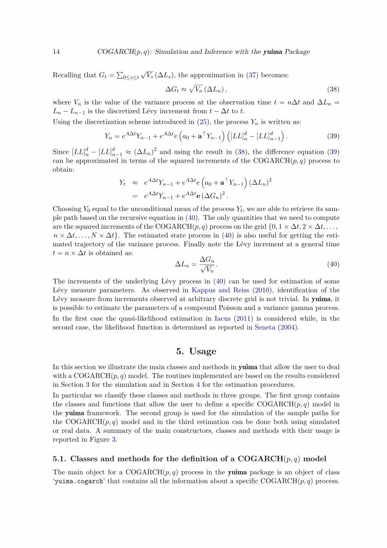


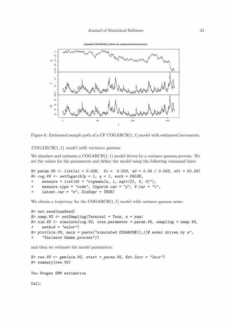


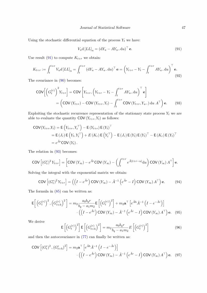


![[XLS]bicasociety.orgbicasociety.org/cogarch/architectures.xls · Web viewSheet3 Sheet2 Sheet1 ACT-R Soar Clarion Leabra rules, operators declarative Epic GLAIR Alexei Samsonovich](https://static.documents.pub/doc/80x56/5b3569d27f8b9a8b4b8d0b10/xls-web-viewsheet3-sheet2-sheet1-act-r-soar-clarion-leabra-rules-operators.jpg)


