Acknowledgments Grants from the Agricultural Development Board through the Kentucky Horticulture Council have allowed an expansion of the field research and demonstration program to meet the informational and educational needs of our growing vegetable and fruit industries. Important note to readers: The majority of research reports in this volume do not include treatments with experimental pesticides. It should be understood that any experimental pesticide must first be labeled for the crop in question before it can be used by growers, regardless of how it might have been used in research trials. The most recent product label is the final authority concerning application rates, precautions, harvest intervals, and other relevant information. Contact your county’s Cooperative Extension Service if you need assistance in interpreting pesticide labels. This is a progress report and may not reflect exactly the final outcome of ongoing projects. Please do not reproduce project reports for distribution without permission of the authors. Mention or display of a trademark, proprietary product, or firm in text or figures does not constitute an endorsement and does not imply approval to the exclusion of other suitable products or firms. 2007 Fruit and Vegetable Crops Research Report Edited by Timothy Coolong, John Snyder, and Chris Smigell Faculty, Staff, Students, and Grower/Cooperators Horticulture Faculty Doug Archbold Timothy Coolong Tom Cottrell Terry Jones S. Kaan Kurtural Joseph Masabni John Snyder John Strang Mark Williams Area Extension Associates Courtney Flood, Princeton, western Kentucky (vegetables) Nathan Howard, Green River, northwestern Kentucky (vegetables) Nathan Howell, Mammoth Cave, south-central Kentucky (vegetables) Bonnie Sigmon, Laurel and surrounding counties, southeastern Kentucky (vegetables) Chris Smigell, Bluegrass, central Kentucky (small fruits) Dave Spalding, Bluegrass, central Kentucky (vegetables) Horticulture Farm Manager Darrell Slone Horticulture Farms Staff and Technical Staff Katie Bale Sherri Dutton Philip Ray Hays Brandon Henson June Johnston Derek Law Dave Lowry Brandon O’Daniel Janet Pfeiffer Kirk Ranta Hilda Rogers Bonka Vaneva David Wayne Patsy Wilson Dwight Wolfe Graduate Students Audrey Horrall Shawn Lucas Janet Meyer Katie Russell Delia Scott Patsy Wilson International Student Interns (Thailand) Danurit Supamoon Ekkapot Boonnu Horticulture Farm Temporary Staff and Student Workers Ben Abell Katie Arambasick Matt Anderson Jessica Ballard Charles Bobrowski Ryan Capito Daniel Carpenter Jessica Cole Carolyce Dungan Chris Fuehr Lucas Hanks Ben Henshaw Erin Kunze Jacquelyn Neal Tyler Pierce Amy Posten Peter Sahajian Kiefer Shuler Matthew Simson Joseph Tucker Plant Pathology Faculty John Hartman Kenny Seebold Professional Staff Paul Bachi Julie Beale Ed Dixon Sara Long Agricultural Economics Faculty Wuyang Hu Tim Woods Nutrition/Food Science Faculty Sandra Bastin Extension Agents for Ag and Horticulture (county research sites) Amy Aldenderfer, Hardin Co. Ronald Bowman, Nelson Co. Gary Carter, Harrison Co. Jeffrey Casada, Clay Co. Joanna Coles, Warren Co. Jamie Dockery, Fayette Co. Jack Ewing, Grayson Co. Clint Hardy, Daviess Co. Dr. Annette Heisdorffer, Daviess Co. Greg Henson, McLean Co. Frank Hicks, Clark Co. Kelly Jackson, Christian Co. Edward Lanham, Marion Co. Josh Long, Fayette Co. Diane Perkins, Hancock Co. Jeff Porter, Henderson Co. Rankin Powell, Union Co. Carol Schreiber, Warren Co. Douglas Shephard, Hardin Co. Robert Smith, Nelson Co. Regulatory Services Soil Testing Lab Frank Sikora Kentucky State University Faculty George F. Antonious (Dept. of Plant and Soil Sciences) Kirk Pomper (Dept. of Plant and Soil Sciences) Small Farm Outreach Louie Rivers Harold Eli Professional Staff Sherry Crabtree Jeremiah Lowe Zachary Ray Berea College Faculty Sean Clark (Dept. of Agriculture and Natural Resources) Student Researchers Miranda Hileman Grower/Cooperators Zeldon Angel John Bell Kevin Bland Charlene Bowling Butch Case Tim Cecil Chris Coulter Shauna Davis Darrell and Donna Foster Laura Garrison Bruce Gibson Fred and Alison Gibson Bethany Hardcastle Kyle Hayden Kris Johnson Tolman Mills James Murdock Larry Thomas Aaron Walker David Weaver
Transcript
AcknowledgmentsGrants from the Agricultural Development Board through the Kentucky Horticulture Council have allowed an expansion of the field research and demonstration program to meet the informational and educational needs of our growing vegetable and fruit industries.
Important note to readers:The majority of research reports in this volume do not include treatments with experimental pesticides. It should be understood that any experimental pesticide must first be labeled for the crop in question before it can be used by growers, regardless of how it might have been used in research trials. The most recent product label is the final authority concerning application rates, precautions, harvest intervals, and other relevant information. Contact your county’s Cooperative Extension Service if you need assistance in interpreting pesticide labels.
This is a progress report and may not reflect exactly the final outcome of ongoing projects. Please do not reproduce project reports for distribution without permission of the authors.
Mention or display of a trademark, proprietary product, or firm in text or figures does not constitute an endorsement and does not imply approval to the exclusion of other suitable products or firms.
2007 Fruit and Vegetable Crops Research ReportEdited by Timothy Coolong, John Snyder, and Chris Smigell
Professional StaffPaul BachiJulie BealeEd DixonSara Long
Agricultural EconomicsFaculty Wuyang HuTim Woods
Nutrition/Food ScienceFacultySandra Bastin
Extension Agents for Ag and Horticulture (county research sites)Amy Aldenderfer, Hardin Co.Ronald Bowman, Nelson Co.Gary Carter, Harrison Co.Jeffrey Casada, Clay Co.Joanna Coles, Warren Co.Jamie Dockery, Fayette Co.Jack Ewing, Grayson Co.Clint Hardy, Daviess Co. Dr. Annette Heisdorffer, Daviess Co. Greg Henson, McLean Co.Frank Hicks, Clark Co.Kelly Jackson, Christian Co.Edward Lanham, Marion Co.Josh Long, Fayette Co.Diane Perkins, Hancock Co. Jeff Porter, Henderson Co. Rankin Powell, Union Co. Carol Schreiber, Warren Co.Douglas Shephard, Hardin Co.Robert Smith, Nelson Co.
Regulatory Services Soil Testing LabFrank Sikora
Kentucky State UniversityFaculty George F. Antonious (Dept. of
Plant and Soil Sciences)Kirk Pomper (Dept. of Plant and
Soil Sciences)
Small Farm OutreachLouie RiversHarold Eli
Professional StaffSherry CrabtreeJeremiah LoweZachary Ray
Berea CollegeFacultySean Clark (Dept. of Agriculture
and Natural Resources)
Student ResearchersMiranda Hileman
Grower/Cooperators Zeldon AngelJohn BellKevin BlandCharlene BowlingButch CaseTim CecilChris CoulterShauna DavisDarrell and Donna FosterLaura GarrisonBruce GibsonFred and Alison GibsonBethany HardcastleKyle HaydenKris JohnsonTolman MillsJames MurdockLarry ThomasAaron WalkerDavid Weaver
ContentsIntroduction2007 Fruit and Vegetable Crops Research Report .............................................................................1UK Fruit and Vegetable Program Overview—2007 ........................................................................5Getting the Most Out of Research Reports .........................................................................................6Retail Demand for Blueberry Vinegar and Blueberry Syrup ...................................................... 10
DemonstrationsOn-Farm Vegetable Demonstrations in Northwestern Kentucky ........................................... 11On-Farm Commercial Vegetable and Chrysanthemum Demonstrations
in South-Central Kentucky ......................................................................................................... 12On-Farm Commercial Vegetable Demonstrations in Southeastern Kentucky .................. 13On-Farm Commercial Vegetable Demonstration.......................................................................... 15
Grapes and WineKentucky Viticultural Regions and Suggested Cultivars .............................................................. 162000 Wine Grape Cultivar Trial ............................................................................................................ 18Effect of Pruning Formula on Yield and Fruit Composition
of Traminette Grapevines ............................................................................................................ 19Effect of Training Systems on Vine Size, Yield Components, and
Fruit Composition of European Grapevines ........................................................................ 21Effect of Pruning and Cluster Thinning on Crop Load and Coldhardiness
of Vidal Blanc Grapevines............................................................................................................ 23Effects of Pruning and Cluster Thinning on Microclimate, Yield, and
Fruit Composition of Vidal Blanc Grapevines ..................................................................... 26Effect of Crop Load on Vigor, Yield, Fruit Composition, and Wine Phenolics
of Vidal Blanc Grapevines............................................................................................................ 29A Comparison of Ectoparasitic Nematode Populations in American and
French-American Hybrid Grapevines .................................................................................... 32Impact of Japanese Beetle Defoliation on the Overwintering Ability
of First-Year Grapevines ............................................................................................................... 35Evaluation of Matrix in Dormant Grape............................................................................................ 36
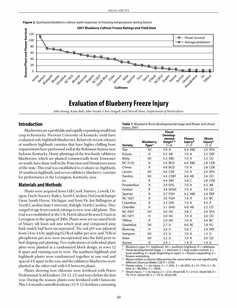
Small FruitsBlueberry Cultivar Freeze Tolerance for Eastern Kentucky ....................................................... 39Evaluation of Blueberry Freeze Injury................................................................................................. 40Weed Control in Bearing Blueberry .................................................................................................... 41The Kentucky Primocane-Fruiting Blackberry Trial ..................................................................... 42Evaluation of Strawberry Varieties as Matted Rows ...................................................................... 43Plasticulture Strawberry Variety Evaluation ..................................................................................... 45High Tunnel and Field Plasticulture Strawberry Evaluation....................................................... 46Optimizing Organic Culture of Select Small Fruits in Kentucky
Using Haygrove Tunnels .............................................................................................................. 47
Tree FruitsRootstock and Interstem Effects on Pome Fruit Trees ................................................................. 50Establishment of an Organic Apple Orchard at the UK Horticulture Research Farm ..... 52Evaluation of Casoron in Bearing Apple ............................................................................................ 54
VegetablesRomaine Lettuce Cultivar Trial ............................................................................................................. 55Spring Greens and Lettuce Variety Evaluations .............................................................................. 56Financial Analysis of Small-Scale, Organic, Cut-Lettuce Production Systems .................... 61Supersweet Corn Evaluations in Central Kentucky ....................................................................... 63Supersweet Corn Evaluations in Eastern Kentucky, 2007 ........................................................... 64Comparison of Preemergence and Postemergence Herbicides in Sweet Corn .................. 65Specialty Melon Variety Evaluations ................................................................................................... 67Seedless and Seeded Watermelon Variety Evaluations ................................................................ 70Yield and Income of Fall Staked Tomato Cultivars in Eastern Kentucky .............................. 72Evaluation of Fungicide Programs for Management of Diseases of Staked Tomato ......... 74Season Extension of Tomatoes Using High Tunnel Technology in Eastern Kentucky ..... 76Evaluation of Application of Command and Treflan under Plastic Mulch
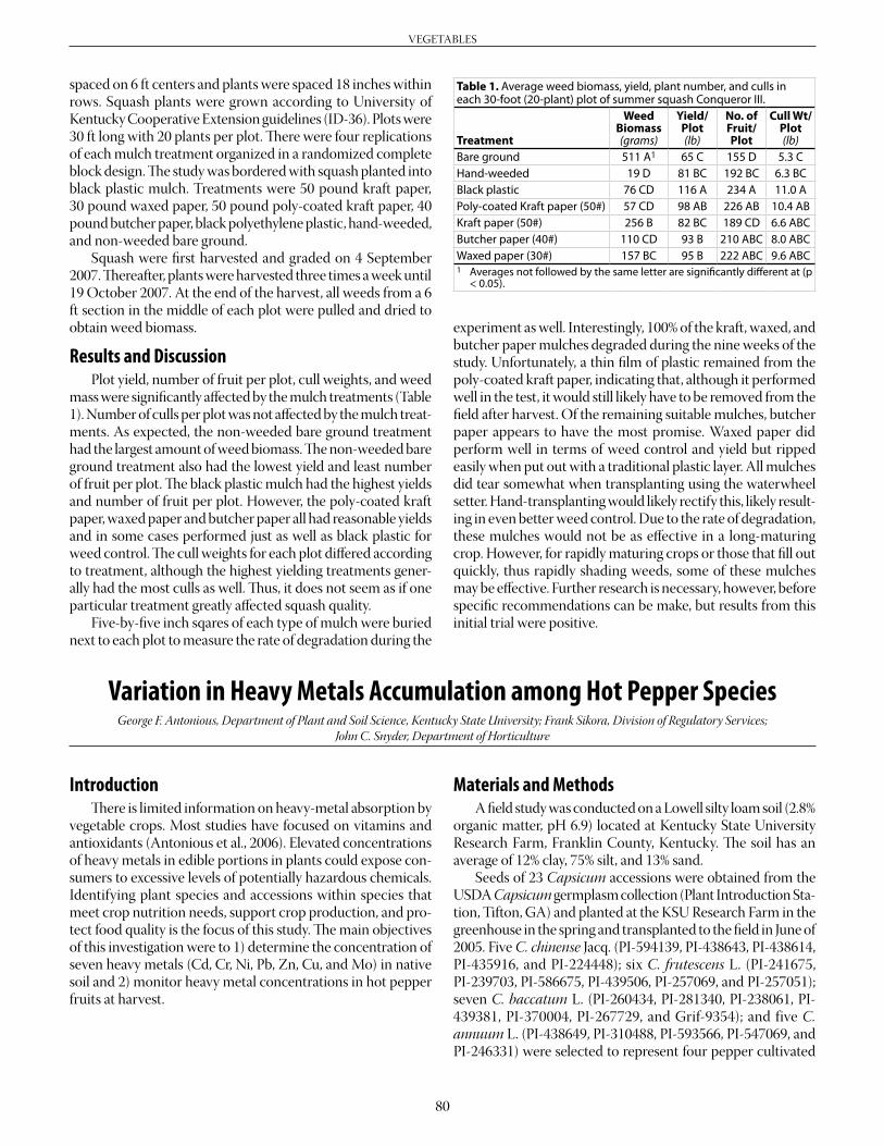
for Pepper Production ................................................................................................................... 77Evaluation of Sandea at Three Transplanting Times in Three Cucurbit Crops ................... 78Performance of Paper Mulches for Weed Control in Summer Squash .................................. 79Variation in Heavy Metals Accumulation among Hot Pepper Species .................................. 80Sewage Sludge and Productivity of Vegetables Grown on Erodible Lands .......................... 82Sewage Sludge Reduces Dimethoate Residues in Runoff Water .............................................. 85Evaluation of Callisto for Crop Safety in Sweet Sorghum............................................................ 87
Diagnostic LaboratoryFruit and Vegetable Disease Observations from the Plant Disease
Appendix A: Sources of Vegetable Seeds .......................................................................................... 91
5
INTRODUCTION
UK Fruit and Vegetable Program Overview—2007 Dewayne Ingram, Chair, Department of Horticulture
The UK Fruit Crops and Vegetable Crops Programs are the coordinated efforts of faculty, staff, and students in several departments in the College of Agriculture for the benefit of the Kentucky fruit and vegetable industries. Our 2007 report is divided into sections providing information on on-farm demonstrations; the results of research projects involving small fruits, tree fruits, and vegetables; and observations from the plant diagnostic laboratory. Research projects reported here reflect stated industry needs, expertise available at UK, and the nature of research projects around the world generating information applicable to Kentucky. If you have questions or suggestions about a particular research project, please do not hesitate to contact us. Funds from the Agricultural Development Board through Kentucky Horticulture Council grants and the Kentucky Grape and Wine Council, as well as U.S. Department of Agriculture grants for the New Crop Opportunities Center have allowed us to double the number of field research plots statewide in recent years. This has occurred during a time of rapid industry growth and emergence of vital questions about our production and marketing systems. These grants have also funded Extension Associates, located throughout the state, who are helping new and existing grow-ers understand and apply the technologies of more profitable production and marketing systems. On-farm demonstrations, on-farm consulting, and collaboration with county Extension agents have been the hallmark of this program. The investment in this approach is paying great dividends, as I think you will see in the results presented here. Implementation of our plans to improve the Horticulture Research Farm (South Farm) is progressing. This year we have finished a headhouse for the greenhouse complex and erected six research greenhouses that we expect to be operational in early 2008. We now have 3 acres of grape research plots and expanded blackberry and blueberry plots there. An 11-acre parcel is now certified organic, which will allow us to perform research for organic farmers in Kentucky. The grant funds have also allowed us to maintain an expand-ed vegetable and fruit research program at the research farms in Princeton and Quicksand. Research plots on the reclaimed mine land in eastern Kentucky generated valuable information but have been terminated due to vandals. Watch for the announcement of field days at the Horticul-ture Research Farm in Lexington and at Robinson Station in Quicksand in 2008. The field day at Princeton in 2007 was a great success, with great weather and high attendance.
Although the purpose of this publication is to report re-search results and summarize our Extension program results, we have also highlighted below some of our undergraduate and graduate degree programs.
Undergraduate Program Highlights The department offers areas of emphasis in Horticultural Enterprise Management and Horticultural Science within a Horticulture, Plant, and Soil Science Bachelor of Science de-gree. We have also taken the lead in establishing a B.S. degree in Sustainable Agriculture. Following are a few highlights of our undergraduate horticulture program in 2006-2007: The Horticulture, Plant and Soil Science degree program has nearly 100 students for the fall semester of 2007, of which almost one-half are Horticulture students and another one-third are turfgrass students. Twelve horticulture students graduated in the 2006-2007 academic year. We believe that a significant portion of an undergraduate education in horticulture must come outside the classroom. In addition to the local activities of the Horticulture Club and field trips during course laboratories, students have excellent off-campus learning experiences. Here are the highlights of such opportunities in 2006.• Fifteenstudentsparticipatedina12-daystudytourtoJapan
in May led by Drs. Robert McNiel, Robert Geneve, and Tom Nieman.
• Horticulturestudentscompetedinthe2007ProfessionalLandcare Network (PLANET) Career Day competition at Michigan State University in March (Drs. Robert McNiel and Robert Geneve, faculty advisors).
• Studentsaccompanied faculty to the followingregional/national/internationalmeetings, including theAmericanSociety for Horticultural Science Annual Conference, Eastern Region—International Plant Propagators’ Society, the Kentucky Landscape Industries Conference, Southern Nursery Association Research Conference and Trade Show, and the Mid-States Horticultural Expo.
Graduate Program Highlights The demand for graduates with M.S. or Ph.D. degrees in Horticulture, Entomology, Plant Pathology, and Agricultural Economics is high. Our M.S. graduates are being employed in the industry, Cooperative Extension Service, secondary and postsecondary education, and governmental agencies. Gradu-ate students are active participants in the fruit and vegetable commodity teams and contribute significantly to our ability to address problems and opportunities important to Kentucky.
6
INTRODUCTION
Getting the Most Out of Research ReportsTimothy Coolong, John Snyder, and Brent Rowell (Adjunct Professor), Department of Horticulture
The 2007 Fruit and Vegetable crops research report includes results of more than 45 field research trials that were conducted in 16 counties in Kentucky (see map, below). Research was conducted by faculty and staff from several departments within the University of Kentucky College of Agriculture, including Horticulture, Plant Pathology, Agricultural Economics, and Nutrition and Food Science. This report also includes collab-orative research projects conducted with faculty and staff at Kentucky State University and Berea College. Many of these reports include data on varietal performance as well as differ-ent production methods, in an effort to provide growers with better tools that they can use to improve fruit and vegetable production in Kentucky. Variety trials included in this year’s publication include watermelons and specialty melons, strawberries, blueberries, lettuce and greens, sweet corn, grapes, apples, and tomatoes. New varieties are continually being released, and variety trials provide us with much of the information necessary to update our recommended varieties in our Vegetable Production Guide for Commercial Growers (ID-36). However, when making de-cisions about what varieties to include in ID-36, we factor in performance at multiple locations in Kentucky over multiple years. We may also collaborate with researchers in surrounding states to discuss results of variety trials they have conducted. In addition, we also consider such things as seed availability, which is often of particular concern for organic growers. Only then, after much research and analysis, will we make variety recommendations for growers in Kentucky. The results pre-sented in this publication often reflect a single year of data at a limited number of locations. Although some varieties perform well across Kentucky year after year, others may not. Here are some helpful guidelines for interpreting the results of fruit and vegetable variety trials.
Our Yields vs. Your Yields Yields reported in variety trial results are extrapolated from small plots. Depending on the crop, our trial plot sizes range anywhere from 50 to 500 sq ft. Yields per acre are calculated by multiplying these small plot yields by correction factors rang-ing from 100 to 1,000. For example, if there are typically 4,200 tomato plants per acre when using recommended planting densities, and our study includes only 50 plants per plot, our yield data from those 50 plants will be multiplied by a factor of 84 to generate per acre yields. Thus, small errors can be ampli-fied when correction factors are used. Often, because plots that are harvested do not include such things as drive rows, per acre yields in research plots may be much higher than those in a typical grower’s field. Additionally, in many cases, research plots may be harvested more often than is economically feasible in a grower’s field. Thus, do not be surprised if our reported yields are much higher than yours. Also, while absolute yields are im-portant, variety trials generally compare a number of varieties to an industry standard for that crop. Thus, we are often interested in the relative performance of varieties to that standard. If one variety consistently underperforms when compared to the standard variety, then we will generally not recommend using it unless it meets a specific market niche for some growers. It is best not to compare the yield of a variety at one location to the yield of a different variety at another location. The dif-ferences in performance among all varieties grown at the same location, however, can and should be used to identify the best varieties for growers nearest that locality. Results vary widely from one location or geographical region to another; a variety may perform well in one location and poorly in another for many reasons. Different locations may have different climates, microclimates, soil types, fertility regimes, and pest problems. Different trials at different locations are also subject to differ-ing management practices. Only a select few varieties seem to perform well over a wide range of environmental conditions, and these varieties usually become top sellers. Climatic conditions obviously differ considerably from one season to the next, and it follows that some varieties perform well one year and perform poorly the next. For this reason, we prefer to have at least two years of trial data before coming to any hard and fast conclusions about a variety’s performance. In other cases, we may conduct a preliminary trial to eliminate the worst varieties and let growers make the final choices regard-ing the best varieties for their farm and market conditions (see Rapid Action Cultivar Evaluation [RACE] trial description on page 9).
Making Sense of Statistics Most trial results use statistical techniques to determine if there are any real (versus accidental) differences in perfor-mance among varieties or treatments. Statistical jargon is often a source of confusion, and we hope this discussion will help. To apply statistical analysis, our trials must be replicated. Gener-ally, they will be replicated in several plots at a single location. For example, if we have a trial with 20 pepper varieties, we will have a small plot (20 to 30 plants) for each variety (20 separate plots) and then repeat this planting in two or three additional sets of 20 plots in the same trial field. These repeated sets of the same varieties are called replications or blocks. The result is a field trial with 20 varieties x 4 replications = 80 small plots. The performance of each plot will then be recorded and combined with data from the other plots of that variety to get an average (also called the mean) of yields for that variety. The average per acre yields reported in the tables are calculated by multiplying these average small plot yields by a correction factor.
Statistically Different—Not Just Different In most reports, we list the results in tables with varieties ranked from highest to lowest yielding, from earliest to latest maturing, or for which property is most important for that crop. Often yields will be followed by a letter. Typically, varieties with yields followed by different letters are statistically differ-ent. For example, in Table 1, if X3R Aristotle bell peppers yield 25tons/acreandKingArthurbellpeppersyield22tons/acrebut are followed by the same letter, then they are no different, despite seeming to have a large difference in yield. The reason for this is that there is often variation between plots in study. The yields reported in ables are averages of several plots. Thus, four plots of X3R Aristotle peppers could have yielded 30, 20, 23,and27tons/acre.Althoughtheaverageis25tons/acre,theyieldsactuallyrangedfrom20to30tons/acre.TheKingArthurpepperscouldhaveaveraged22tons/acrebuthadplotyieldsof18,22,25,and21tons/acre.Thus,whiletheaveragesappeardifferent, there was actually some overlap in yield for the two
Table 1. Yields, gross returns, and appearance of bell pepper cultivars under bacterial spot-free conditions in Lexington, Kentucky; yield and returns data are means of four replications.
Cultivar Seed
Source
Tot. Mkt. Yield1
(tons/A)% XL
+Large2Income3
($/acre)Shape Unif.4
Overall Appear.5
No. Lobes6
Fruit Color Comments
X3R Aristotle S 25 a 89 10180 4 7 3 dk green most fruits longer than wide King Arthur S 22.5 a 88 9079 3 5 4 light-med green deep blossom-end cavities 4 Star RG 22.2 a 86 9111 3.5 6 4 light-med green Boynton Bell HM 21.7 a 92 9003 3 5 3 med-dk green ~15% of fruits 2-lobed (pointed) Corvette S 20.6 a 88 8407 3 6 3&4 med-dk green ~10% elongated (2-lobed) X3R Red Knight S 20.5 a 90 8428 3 5 4 med-dk green SP 6112 SW 20.2 a 78 8087 4 6 3 med green Conquest HM 20 a 85 8021 2 5 3&4 light-med green deep stem-end cavities, many
misshapen Orion EZ 20 a 93 8219 4 6 4 med-dk green Lexington S 19.8 a 87 8022 3.5 6 3 dk green PR99Y-3 PR 19.5 b 87 7947 3 5 3&4 med green many misshapen fruits Defiance S 18.7 b 87 7568 4 7 3&4 dk green X3R Ironsides S 18.4 b 92 7585 4 6 3 med green ~5% w/deep stem-end cavities X3R Wizard S 18 b 92 7447 3 6 3&4 dk green RPP 9430 RG 17.3 b 89 7029 3 6 4 med-dk green ~10% of fruits elongated ACX 209 AC 17.2 b 89 7035 3.5 6 3 med green
Waller-Duncan LSD (P < 0.05) 5.2 7 2133 1 Total marketable yield included yields of U.S. Fancy and No. 1 fruits of medium (greater than 2.5 in. diameter) size and larger plus misshapen but sound
fruit that could be sold as “choppers” to foodservice buyers. 2 Percentage of total yield that was extra-large (greater than 3.5 in. diameter) and large (between 3 and 3.5 in. diameter). 3 Income = gross returns per acre; average 2000 season local wholesale prices were multiplied by yields from different size/grade categories: $0.21/lb for
extra-large and large, $0.16/lb for mediums, and $0.13/lb for “choppers,” i.e., misshapen fruits. 4 Average visual uniformity of fruit shape where 1 = least uniform, 5 = completely uniform. 5 Visual fruit appearance rating where 1 = worst, 9 = best, taking into account overall attractiveness, shape, smoothness, degree of flattening, color, and
shape uniformity; all fruits from all four replications observed at the second harvest (July 19). 6 3&4 = about half and half 3- and 4-lobed; 3 = mostly 3-lobed; 4 = mostly 4-lobed.
8
INTRODUCTION
varieties; therefore, they are not statistically different. When possible, readers should look at the variation in some varieties or tests. The amount of variation present will either be listed as standard deviation or standard error. The higher the amount of error or deviation, the more variation there is for that variety or treatment. Readers should be wary of choosing varieties with high levels of standard deviation (greater than 25% of the aver-age of that variety), as those varieties may be highly variable in the field. The best varieties not only perform well but have little variation. Sometimes numbers in tables will be followed by several let-ters. For example, if in a tomato trial Mountain Spring tomatoes have yield data followed by the letters AB, then their average yield is not significantly different from the highest yielding varieties (those followed by an A) or lower yielding varieties (those fol-lowed by a B). This means that the yield of Mountain Spring was intermediate between other varieties and that there was enough variation to ensure that statistically they were no different from varieties followed by an A and those followed by a B.
Least Significant Difference (LSD) The last line at the bottom of most data tables will usually contain a number that is labeled LSD, or Waller-Duncan LSD. LSD is a statistical measure that stands for “Least Significant Difference.” The LSD is the minimum yield difference that is required between two varieties before we can conclude that one actu-ally performed better than another. This number enables us to separate real differences among the varieties from chance dif-ferences. When the difference in yields of two varieties is less than the LSD value, we can’t say with any certainty that there is any real yield difference. In other words, we conclude that the yields are the same. For example, in Table 1 cited above, variety X3R Aristotle yielded 25 tons per acre and Boynton Bell yielded 21.7 tons per acre. Since the difference in their yields (25 - 21.7 = 3.3 tons per acre) is less than the LSD value of 5.2 tons per acre, there was no real difference between these two yields. The difference between X3R Aristotle and X3R Wizard (25 - 18 = 7), however, is greater than the LSD, indicating that the difference between the yields of these two varieties is real. What is most important to growers is to identify the best varieties in a trial. What we usually recommend is that you identify a group of best performing varieties rather than a single variety. This is easily accomplished for yields by subtracting the LSD from the yield of the top yielding variety in the trial. Variet-ies in the table having yields equal to or greater than the result of this calculation will belong in the group of highest yielding varieties. If we take the highest yielding pepper variety, X3R Aristotle, in Table 1 and subtract the LSD from its yield (25 - 5.2 = 19.8), this means that any variety yielding 19.8 tons per acre or more will not be statistically different from X3R Aristotle. The group of highest yielding varieties in this case will include the 10 varieties from X3R Aristotle down the column through variety Lexington.
In some cases, there may be a large difference between the yields of two varieties, but this difference is not real (not statis-tically significant) according to the statistical procedure used. Such a difference can be due to chance, but often it occurs if there is a lot of variability in the trial. An insect infestation, for example, could affect only those varieties nearest the field’s edge where the infestation began. It is also true that our customary standard for declaring a statistically significant difference is quite high, or stringent. Most of the trial reports use a standard of 95 percent probability (expressed in the tables together with the LSD as P<0.05 or P = 0.05). This means that there is a 95 percent probability that the difference between two yields is real and not due to chance or error. When many varieties are compared (as in the pepper example above), the differences between yields of two varieties must often be quite large before we can conclude that they are really different. After the group of highest yielding, or in some cases, highest income,1 varieties (see Table 1 cited above) has been identified, growers should select varieties within this group that have the best fruit quality (often the primary consideration), best disease resistance, or other desirable trait for the particular farm envi-ronment and market outlet. One or more of these varieties can then be grown on a trial basis on your farm using your cultural practices.
RACE Trials In cases where there are too many new varieties to test economically or when we suspect that some varieties will likely perform poorly in Kentucky, we may decide to grow each vari-ety in only a single plot for observation. In this case, we cannot make any statistical comparisons but can use the information obtained to eliminate the worst varieties from further testing. We can often save a lot of time and money in the process. We can also provide useful preliminary information to growers who want to try some of these varieties in their own fields. Since there are so many new marketing opportunities these days for such a wide variety of specialty crops, we have decided that this single-plot approach for varieties unlikely to perform well in Kentucky is better than providing no information at all. We hope that RACE trials will help fill a need and best use limited resources at the research farms.
______________________1 It is often desirable to calculate a gross “income” or gross return for
vegetable crop varieties that will receive different market prices based on when they are harvested (earliness) and on pack-out of different fruit sizes and grades (bell peppers, tomatoes, cucumbers). In these cases, for a given harvest date, yields in each size class/grade are multiplied by their respective market prices on that date to determine gross returns (= income) for each cultivar in the trial.
9
INTRODUCTION
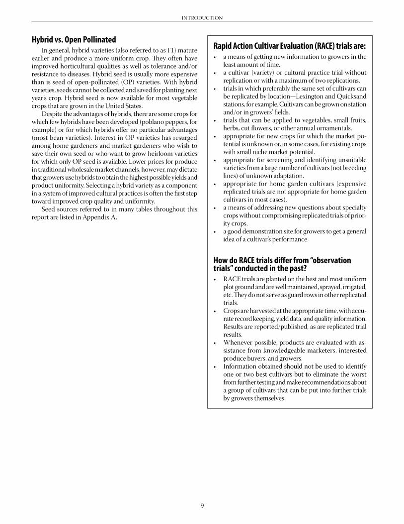
Hybrid vs. Open Pollinated In general, hybrid varieties (also referred to as F1) mature earlier and produce a more uniform crop. They often have improvedhorticulturalqualitiesaswell as toleranceand/orresistance to diseases. Hybrid seed is usually more expensive than is seed of open-pollinated (OP) varieties. With hybrid varieties, seeds cannot be collected and saved for planting next year’s crop. Hybrid seed is now available for most vegetable crops that are grown in the United States. Despite the advantages of hybrids, there are some crops for which few hybrids have been developed (poblano peppers, for example) or for which hybrids offer no particular advantages (most bean varieties). Interest in OP varieties has resurged among home gardeners and market gardeners who wish to save their own seed or who want to grow heirloom varieties for which only OP seed is available. Lower prices for produce in traditional wholesale market channels, however, may dictate that growers use hybrids to obtain the highest possible yields and product uniformity. Selecting a hybrid variety as a component in a system of improved cultural practices is often the first step toward improved crop quality and uniformity. Seed sources referred to in many tables throughout this report are listed in Appendix A.
least amount of time. • acultivar (variety)orculturalpractice trialwithout
replication or with a maximum of two replications.• trialsinwhichpreferablythesamesetofcultivarscan
be replicated by location—Lexington and Quicksand stations, for example. Cultivars can be grown on station and/oringrowers’fields.
• trials thatcanbeapplied tovegetables, small fruits,herbs, cut flowers, or other annual ornamentals.
• appropriate fornewcrops forwhichthemarketpo-tential is unknown or, in some cases, for existing crops with small niche market potential.
• appropriate forscreeningand identifyingunsuitablevarieties from a large number of cultivars (not breeding lines) of unknown adaptation.
• appropriate for home garden cultivars (expensivereplicated trials are not appropriate for home garden cultivars in most cases).
• ameansofaddressingnewquestionsaboutspecialtycrops without compromising replicated trials of prior-ity crops.
• agooddemonstrationsiteforgrowerstogetageneralidea of a cultivar’s performance.
How do RACE trials differ from “observation trials” conducted in the past?• RACEtrialsareplantedonthebestandmostuniform
plot ground and are well maintained, sprayed, irrigated, etc. They do not serve as guard rows in other replicated trials.
• Cropsareharvestedattheappropriatetime,withaccu-rate record keeping, yield data, and quality information. Resultsarereported/published,asarereplicatedtrialresults.
• Wheneverpossible,productsareevaluatedwithas-sistance from knowledgeable marketers, interested produce buyers, and growers.
• Informationobtainedshouldnotbeusedtoidentifyone or two best cultivars but to eliminate the worst from further testing and make recommendations about a group of cultivars that can be put into further trials by growers themselves.
10
INTRODUCTION
A retail demand study was initiated to explore the level of demand and some of the determining factors for certain pro-cessed blueberry products. The products were selected based on their development potential in Kentucky. A retail supermarket intercept survey was designed that included a presentation of prototype formulations and packaging of blueberry basil vinegar and blueberry syrup developed with assistance from the UK Food Science Department. The results provide a better basis for understanding the market for these products in Kentucky and a framework for developing future pricing strategies. A total of 604 consumers were surveyed in four retail mar-kets around Kentucky. Surveys were randomized by product subject to limit length since a relatively large number of blue-berry products were being investigated. Consumers were pre-sented with a reference price range of comparable products in the store and then asked to indicate whether or not they wished to buy this product at all and, if so, how much they were willing to pay. Table 1 provides the results of the consumers’ responses to the vinegar and syrup products. More people were willing to pay a positive amount for the syrup as compared to the vinegar, but both products received a fair amount of interest. Both products have similar reference points. On the market, a regular bottle of apple cider vinegar or a regular bottle of maple syrup is typically sold between $2.50 and $4 for a standard bottle of 8 ounces. Table 2 presents the average amount individuals who expressed a willingness to pay a positive amount would likely pay for the two blueberry products. Con-sumers were willing to pay about $0.30 more for the blueberry syrup. Average willingness to pay for both products falls within the range of comparable products available on the market. Blueberry basil vinegar and blueberry syrup are different products having different uses. They were expected to appeal to dif-ferent kinds of customers. Basic demographic data were collected during the survey and used to better understand the determinants of the differences in responses to willingness to pay. The impact of the knowledge of the health attributes of blueberries was included in the analysis. One-half of the surveys included a blueberry health statement, quoting from studies that have shown that antioxidants in blueberries may protect the body against damaging effects of free radicals and chronic diseases associated with aging. Blueberries naturally contain antioxidants such as vitamins C and E, antho-cyanins, and phenolics. This demographic and health knowledge information can help product developers know how and where to position these products to achieve maximum demand. A simple regression model was estimated using willingness to pay (WTP) as the dependent variable and the demographic data as determinants, the independent variables. Table 3 pro-vides a summary of the regression results of whether different individuals may be willing to pay differently for these blueberry products. Detailed regression results are presented in Table 4. The vinegar model can be summarized as follows: 1) Men, compared to women, are willing to pay slightly (although not
significantly) more; 2) younger age groups are willing to pay more than older age groups; 3) individuals with higher incomes are will-ing to pay more; 4) individuals with higher education are willing to pay more; and 5) individuals shown the health statement were willing to pay slightly (although not significantly) more. The syrup model indicates results similar to those for vin-egar, relating to the direction of impact, although in this case the health statement appears to be a much more significant positive factor. This suggests that merchandising strategies such as health attribute labels may have a greater impact on a product like syrup, compared to vinegar.
Retail Demand for Blueberry Vinegar and Blueberry SyrupTimothy Woods and Wuyang Hu, Agricultural Economics; Sandra Bastin and Nick Wright, Nutrition and Food Science
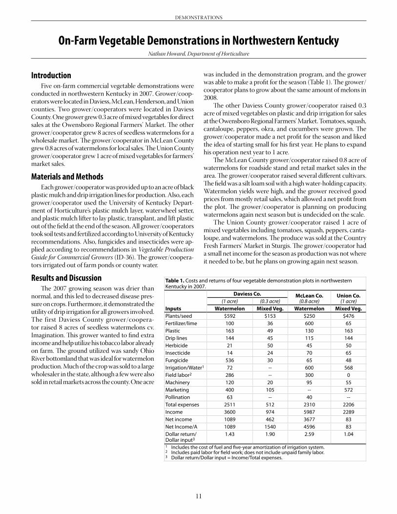
Introduction Five on-farm commercial vegetable demonstrations were conductedinnorthwesternKentuckyin2007.Grower/coop-erators were located in Daviess, McLean, Henderson, and Union counties.Twogrower/cooperatorswere located inDaviessCounty. One grower grew 0.3 acre of mixed vegetables for direct sales at the Owensboro Regional Farmers’ Market. The other grower/cooperatorgrew8acresofseedlesswatermelonsforawholesalemarket.Thegrower/cooperatorinMcLeanCountygrew 0.8 acres of watermelons for local sales. The Union County grower/cooperatorgrew1acreofmixedvegetablesforfarmers’market sales.
Materials and Methods Eachgrower/cooperatorwasprovideduptoanacreofblackplastic mulch and drip irrigation lines for production. Also, each grower/cooperatorusedtheUniversityofKentuckyDepart-ment of Horticulture’s plastic mulch layer, waterwheel setter, and plastic mulch lifter to lay plastic, transplant, and lift plastic outofthefieldattheendoftheseason.Allgrower/cooperatorstook soil tests and fertilized according to University of Kentucky recommendations. Also, fungicides and insecticides were ap-plied according to recommendations in Vegetable Production Guide for Commercial Growers (ID-36).Thegrower/coopera-tors irrigated out of farm ponds or county water.
Results and Discussion The 2007 growing season was drier than normal, and this led to decreased disease pres-sure on crops. Furthermore, it demonstrated the utility of drip irrigation for all growers involved. The firstDaviessCounty grower/coopera-tor raised 8 acres of seedless watermelons cv. Imagination. This grower wanted to find extra income and help utilize his tobacco labor already on farm. The ground utilized was sandy Ohio River bottomland that was ideal for watermelon production. Much of the crop was sold to a large wholesaler in the state, although a few were also sold in retail markets across the county. One acre
On-Farm Vegetable Demonstrations in Northwestern KentuckyNathan Howard, Department of Horticulture
was included in the demonstration program, and the grower wasabletomakeaprofitfortheseason(Table1).Thegrower/cooperator plans to grow about the same amount of melons in 2008. TheotherDaviessCountygrower/cooperatorraised0.3acre of mixed vegetables on plastic and drip irrigation for sales at the Owensboro Regional Farmers’ Market. Tomatoes, squash, cantaloupe, peppers, okra, and cucumbers were grown. The grower/cooperatormadeanetprofitfortheseasonandlikedthe idea of starting small for his first year. He plans to expand his operation next year to 1 acre. TheMcLeanCountygrower/cooperatorraised0.8acreofwatermelons for roadside stand and retail market sales in the area.Thegrower/cooperatorraisedseveraldifferentcultivars.The field was a silt loam soil with a high water-holding capacity. Watermelon yields were high, and the grower received good prices from mostly retail sales, which allowed a net profit from theplot.Thegrower/cooperator isplanningonproducingwatermelons again next season but is undecided on the scale. TheUnionCounty grower/cooperator raised1 acreofmixed vegetables including tomatoes, squash, peppers, canta-loupe, and watermelons. The produce was sold at the Country FreshFarmers’MarketinSturgis.Thegrower/cooperatorhada small net income for the season as production was not where it needed to be, but he plans on growing again next season.
Table 1. Costs and returns of four vegetable demonstration plots in northwestern Kentucky in 2007.
1 Includes the cost of fuel and five-year amortization of irrigation system.2 Includes paid labor for field work; does not include unpaid family labor.3 Dollar return/Dollar input = Income/Total expenses.
12
DEMONSTRATIONS
On-Farm Commercial Vegetable and Chrysanthemum Demonstrations in South-Central Kentucky
Nathan Howell, Department of Horticulture
Introduction Five on-farm commercial veg-etable and chrysanthemum dem-onstrations were conducted in south-centralKentucky.Grower/cooperators for the demonstra-tions were located in Grayson, Hardin, and Warren counties. The cooperator in Grayson County had a demonstration plot of ap-proximately 0.17 acre consisting of Mountain Fresh Plus and heirloom tomatoes. The cooperator mar-keted his produce at the Southern Kentucky Regional Farmers’ Mar-ket in Bowling Green, Kentucky, regional restaurants, and grocery stores. Two on-farm demonstrations were located in Hardin County. One demonstration plot was ap-proximately 0.18 acre consisting of Goliath and Jetstar tomatoes that were marketed at the Eliza-bethtown Farmers’ Market and a roadside market. The second demonstration was 0.66 acre of pumpkins and gourds. The primary planting was Spartan and Trojan varieties of field pumpkins. The cooperator marketed his crop as part of his on-farm entertainment package for school and church groups, which included chrysanthemums and a corn maze. Warren County also had two on-farm demonstrations. One was 0.10 acres of chrysanthemums that were marketed to local landscapers and as a you-dig operation. The second plot was 0.16 acre of mixed vegetables, which included mini-watermelon, cantaloupe,andheirloomtomatoes.Thegrower/cooperatormarketed his product at the Southern Regional Farmers’ Market in Bowling Green, Kentucky.
Materials and Methods Grower/cooperatorsforthedemonstrationplotswerepro-vided with production supplies such as black or white plastic mulch, drip irrigation lines, blue layflat tubing, and fertilizer injectors.Grower/cooperatorswerealsoabletousetheUni-versity of Kentucky Horticulture Department’s equipment for raised-bed preparation and transplanting. Field preparation was followed by fertilizer applications according to soil test results and recommendations provided by the University of Kentucky. Plastic for the demonstrations was laid in March and April, while the plastic mulch for the pumpkin demonstration was laid in June. White plastic mulch
was used for the pumpkin and chrysanthemum demonstrations; the white mulch provided a cooler growing environment for the late-season crops. The remaining plots used the standard black plastic mulch. All the demonstration plots used a munici-pal water source with irrigation runs no longer than 300 ft. A Chemilizer fertilizer injector was used for a precise application of fertilizer in the chrysanthemum demonstration, while the other plots used a Mazzei-type injection system. ThetwoHardinCountygrower/cooperators,alongwiththeGrayson County cooperator, produced their own transplants; thetwoWarrenCountygrower/cooperatorshadlocalgreen-house managers produce their transplants. Demonstrations were planted from the last week of April through the end of May. The two tomato demonstrations were transplanted with 18-inch row spacing; the mixed vegetable demonstration in Warren County also used 18-inch in-row spacing for his tomatoes and watermelon; 24-inch spacing was used for the cantaloupe. The pumpkin demonstration in Hardin County was spaced in row from 24 to 36 inches depending on the size pumpkin being planted. The chrysanthemum demonstration was spaced at 24 inches with some being double rowed. All the demonstration plots had bed rows 6 to 7 ft on center. After plants were established, insecticides were applied to prevent damage from cucumber beetles and other insects. Imidacloprid, endosulfan, and permethrin were used for insect control. Imidacloprid (Admire) was used as a soil drench and was effective for four weeks; the remaining control was achieved
Table 1. Costs and returns from on-farm demonstrations of mixed vegetable, pumpkins, tomato, and mum crops in Grayson, Hardin, and Warren counties, 2007.
Inputs
Grayson Co. (0.17 acre)
Hardin Co. (0.18 acre)
Hardin Co. (0.66 acre)
Warren Co. (0.10 acre)
Warren Co. (0.16 acre)
Tomato Tomato Pumpkin Mums Mixed Veg.Plants/Seeds $130 $239 $180 $158 $225Fertilizer/Lime 72 261 460 70 75Black/White plastic 33 36 150 23 31Drip line 22 24 88 14 21Tomato stakes, pea fence, etc. 50 142 0 0 0Herbicides 0 74 63 0 20Insecticides 50 106 110 0 63Fungicides 150 208 160 11 182Pollination 0 0 0 0 30Machine1 25 132 10 25 30Irrigation2 1000 325 150 185 182Labor3 300 0 130 0 0Market fees 95 130 0 100 150Total expenses 1927 1677 1501 586 1009Income—retail 5500 5736 2007 875 2750Net income 3573 4059 506 289 1741Dollar return/Dollar input 2.85 3.42 1.34 1.49 2.731 Machine rental, fuel and lube, repairs, and depreciation.2 Three-year amortization of irrigation system plus city water cost where applied.3 Does not include unpaid family labor.
13
DEMONSTRATIONS
by alternating insecticides on a weekly basis until harvest. Three weeks after transplanting, Bravo Weather Stick, Mancozeb, and Quadris were applied on the demonstration plots on an alter-nating weekly schedule for disease control. The University of Kentucky’s recommendations from Vegetable Production Guide for Commercial Growers (ID-36) were used for insecticides and fungicides. Fixed coppers were also used in the tomato demonstrations for control of bacterial problems throughout the year. Nova 40 WP was also used in addition to the above spray program to help control powdery mildew in the Hardin Countypumpkindemonstration.Thegrower/cooperatorofthe chrysanthemum demonstration had only one application of Banrot with no application of insecticides. The demonstration plots were irrigated with at least one-acre inch of water per week and fertigated weekly following the University of Kentucky’s recommendations from ID-36. Harvest for the demonstration plots began in late June and was completed by October.
Results and Discussion The 2007 season was unusual in south-central Kentucky; early March saw above-average temperatures in the 80s fol-lowed by a two-week period in mid-April of killing freeze and record low temperatures of 19 degrees. The months of July and August were affected by a severe drought. Record high temperatures were recorded for nearly the entire month of Au-gust. However, field planting was not interrupted, and the drip irrigationsystemsprovedtobeavitalresourceforthegrower/cooperators. All the demonstrations were able to have a lengthy harvest window that had surpassed their previous bare ground production methods. Nevertheless, there were some disappointments. The cooperator in the mixed vegetable demonstration in Warren County saw very poor fruit set and even aborted fruit on his watermelons due to poor pollination. This was primarily due to not having a beehive for pollination. Once bees were introduced into the field, the fruit set problem was corrected. In addition, while chrysanthemums were effectively grown on white plastic mulch, the presence of the mulch and drip tape presented a problem when plants were dug by consumers. It was difficult to harvest the chrysanthemums without damaging
the drip irrigation lines near the roots of the plants. Thus, when the you-dig type chrysanthemums were not all sold at the same time, the drip line had to be repaired many times throughout the harvest. The Hardin County pumpkin demonstration was also produced on white plastic mulch. The white mulch provided a cooler environment for the pumpkin transplants to get estab-lished and grow in the months of July and August. Strategy 2.1 E herbicide was applied as a banded spray between the rows at a rate of 4 pts per acre; however, the field received a flash flood of nearly 4 inches shortly after the application of herbicide. Nevertheless, the Strategy 2.1 E provided moderate control of most weeds. The major weed problem was nutsedge which not only emerged in the row middles but also came through the plastic mulch itself. The problem arose after the field had been transplanted, and plants were in the pre-bloom stage of five to 10 true leaves. The cooperator decided to use Sandea 75 DF as a postemergence control for the nutsedge. The application was applied as an over-the-top spray of the entire field at a rate of ½ oz per acre. The Sandea 75 DF provided excellent control of the nutsedge with minor damage to the pumpkin crop. The primary damage was leaf burn and some early flower drop due to the application. The pumpkin demonstration also saw an early outbreak of powdery mildew which was held in check with Nova 40 WP at a rate of 2.5 oz per acre. However, it was noted that this product did not have as good control as in previous years. The Hardin County tomato demonstration also saw an out-break of bacterial spot. The problem was noted after removing copper from the spray program during early harvest. A fixed copper application with a low re-entry and harvest interval was added back into the spray program, and the problem was held in check with minor fruit loss. This was an issue that was seen throughout the state in 2007. Overall, it was a very productive and profitable year for demonstrators.All thegrower/cooperators areplanning tocontinue their efforts and expand on the knowledge gained in the demonstration plots. All the demonstrators are projecting future growth in their 2008 production plans. The cooperators’ cost and returns are listed in Table 1.
On-Farm Commercial Vegetable Demonstrations in Southeastern KentuckyBonnie Sigmon, Department of Horticulture
Introduction Three on-farm commercial vegetable demonstrations were conductedinsoutheasternKentucky.Allgrower/cooperatorswere located inClayCounty.Twogrower/cooperatorsgrew0.5 acres of mixed vegetables using the plasticulture method (black plastic mulch and trickle irrigation) and marketed their product to customers straight off the farm. The third Clay Countygrower/cooperatorgrew0.75acresofmixedvegetablesusing the plasticulture method and marketed through the Clay CountyFarmers’Market.Thegrower/cooperatorsweresup-
plied the plastic and irrigation supplies for their demonstration as well as the usage of the plastic mulch layer and waterwheel transplanter.Thegrower/cooperatorswerevisitedonaweeklybasis to address any production problems that developed.
Materials and Methods Clay County Mixed Vegetable Demonstration Plot 1 and 2. Soil testing was conducted, and the recommended fertilizer was applied in early spring. One-half of an acre of black plastic along with trickle irrigation was laid on March 30 and April 3.
14
DEMONSTRATIONS
During the following weeks, several different types and varieties of vegetables were both transplanted and direct seeded to have fresh vegetables for sale throughout the season. Clay County Mixed Vegetable Demonstration Plot 3. Soil testing was conducted, and the recommended fertilizer was applied in early spring. Three-quarters of an acre of black plastic along with trickle irrigation was laid on March 29. Dif-ferent vegetables, with multiple varieties of each, were planted on the black plastic throughout the growing season so as to have a steady diverse supply of fresh produce available for sale at the Clay County Farmers’ Market. Transplants were either purchased from local greenhouse growers or grown by the cooperator. Seeds for direct seeding werepurchasedby thegrower/cooperators fromreputableseed companies. The types and varieties of vegetables grown were leftup to thegrower/cooperator to choosebasedontheir customers’ and their own preferences. Fungicides were sprayed on a weekly basis for disease prevention, and integrated pest management techniques were utilized for the control of insects.
Results and Discussion In 2007, farmers experienced an unusually late spring freeze during the first weeks of April. This affected vegetable produc-ers who were planting early in the hopes of getting premium prices for early produce. Plant kill was even evident under polypropylene row covers. Then the state experienced major drought conditions with some areas of the state being as much as 16 inches below normal rainfall. The cost and returns of all three plots are detailed in Table 1. Plot 1. The space between the rows of plastic was seeded with rye grass at a rate of 75 lb per acre and was mowed as need-ed for weed control. This proved to be a very time-consuming operation, but weed control was superior to the other plots. The irrigation water was supplied by a small stream running next to the plot. The mixed vegetables grown by the coopera-tor included tomatoes, green beans, and melons. The plot was successful in generating extra farm income for the producer. Plot 2. A preemergence herbicide was applied between the rows of plastic, but weed control was very poor due to the lack of rainfall after the application. The irrigation water was costly because municipal water was used. The majority of the plastic was used for sweet corn production. The other crops included tomatoes, cabbage, and melons. The plot did provide added income despite the much higher expense of irrigation.
Plot 3. A preemergence herbicide was also used for weed control between the rows of plastic with little success, again due to the lack of needed rainfall to activate the herbicide. The plot was irrigated using municipal water when needed. Thegrower/cooperatorplantedawidevarietyofvegetablesincluding tomatoes, peppers, green beans, and even potatoes under the plastic mulch. The grower was really pleased with the potato production using plastic, stating that the potatoes were larger and easier to harvest than the potatoes the grower also grew using conventional methods. The plot did generate extra income for the producer. Allthreegrower/cooperatorsweregreatlyimpressedbythebenefits of using plastic mulch and trickle irrigation. They all expressed eagerness to grow vegetables in 2008 utilizing these methods to increase both the production and profitability of their operations.
Table 1. Costs and returns of three commercial vegetable demonstration plots conducted in Eastern Kentucky in 2007.
Labor3 0 0 0Machinery4 110 189 267Total expenses 1266 1704 2268Income 1625 2597 3832Net income 359 893 1564Net income per acre 718 1786 3128Dollar return/Dollar input
1.28 1.52 1.68
1 Transplants produced by grower.2 Five-year amortization on irrigation plus water cost.3 Does not included grower’s labor.4 Machinery depreciation, fuel, and repair.
15
DEMONSTRATIONS
On-Farm Commercial Vegetable DemonstrationDave Spalding and Tim Coolong, Department of Horticulture
Introduction Four on-farm commercial vegetable demonstrations were conducted in central and south-central Kentucky in 2007. Grower/cooperatorswerefromFayette,Marion,andNelsoncounties.Thegrower/cooperatorinMarionCountygrew1.5acres of mixed vegetables that were marketed through an on-farmmarket,whilethegrower/cooperatorinFayetteCountywith 2 acres of mixed vegetables marketed through roadside marketsandalocalfarmers’market.Thegrower/cooperatorin Nelson County with about 0.4 acre of mixed vegetables marketed primarily through the local farmers’ market. A fourth on-farm plot was abandoned in midsummer due to a severe traf-fic accident that left the participant unable to tend the plot.
Materials and Methods As inpreviousyears,grower/cooperatorswereprovidedwith black plastic mulch and drip irrigation lines for up to 1.0 acre and the use of the University of Kentucky Horticulture Department’s equipment for raised bed preparation and trans-planting. The cooperators supplied all other inputs, including labor and management of the crop. In addition to identifying and working closely with cooperators, county Extension agents took soil samples from each plot and scheduled, promoted, and coordinated field days at each site. An Extension associate made regular weekly visits to each plot to scout the crop and make appropriate recommendations. The plots were planted into 6-inch-high beds covered with black plastic mulch and drip lines under the plastic in the center of the beds. The beds were planted at the appropriate spacing according to recommendations in the Kentucky Vegetable Production Guide for Commercial Growers (ID-36). Raised beds were 6 ft from center to center. Plots were sprayed with appropriate fungicides and insecticides on an as-need basis, and cooperators were asked to follow the fertigation schedules provided.
Results and Discussion The unusually hot and dry growing season in 2007 contrib-uted to reduced yields and lower quality of the produce that was marketed. The lack of an adequate water supply in conjunction with high temperatures reduced the potential yields consider-ablyfortwoofthethreegrower/cooperators. Thegrower/cooperatorinMarionCountyhadanadequatewater supply, but late-season production was affected by high temperatures, reducing pollination rates and fruit production for late-season crops. The produce was marketed through an on-farm market with great success. This grower will continue
with the on-farm market in the coming year with only minor adjustments to the product mix and a little more emphasis on early-season crop production. The grower in Nelson County was located in an area of extreme drought. This contributed to a reduction in productiv-ity for part of the demonstration plot. Raised beds with plastic mulch and trickle irrigation accounted for only about one-third of a one-acre plot. However, the majority of marketable produce was produced on mulch and drip irrigation. The conditions of thissummerconvincedthegrower/cooperatortoputallfuturevegetable production on the raised beds with trickle irriga-tion. Thegrower/cooperator inFayetteCountyhad2acresofproduce but only had an adequate water supply for 1 acre. As a result, production from later planted crops did not receive adequate water, and yields were significantly diminished. The grower/cooperatorhadhighermarketingcoststhanmostgrow-ers due to the rental of commercial space and the purchase of a businesslicensetosellproduce.Thegrower/cooperatorintendsto plant about the same next year but is adding another water source for future production.
Table 1. Costs and returns for on-farm demonstration plots in central Kentucky.
1 Cost amortized over three years.2 Includes cost of water and five-year amortization of irrigation system.3 Does not include unpaid family labor.
16
GRAPES AND WINE
Kentucky Viticultural Regions and Suggested CultivarsS. Kaan Kurtural and Joseph Masabni, Department of Horticulture
Introduction Grapes grown in Kentucky are subject to environmental stresses that reduce crop yield and quality and injure or kill grapevines. Damaging winter temperatures, late spring frosts, short growing seasons, and extreme summer temperatures frequently occur in Kentucky. Despite the challenging climate, certain species and cultivars of grapes are grown commercially in Kentucky. Climate is defined as the prevailing weather of a geographic region. There are three categories of the climate that prospective vineyardists have to consider: macroclimate, mesoclimate, and microcli-mate. Macroclimate is the climate of a large region of many square miles. For example, the lower Midwest region is characterized by a continental climate where temperatures fluctuate on a day-to-day basis. The macroclimate in Kentucky is characterized as humid and continental with severe winter temperatures and warm summer temperatures. The conditions in these climates are excellent for the growth of annual crops. Most rainfall occurs in the summer months. However, in some years, rainfall is sparse, resulting in drought. Mesoclimate is the climate of a vineyard site as affected by its local topography. The topography of a site, including the absolute elevation, slope, aspect, and soils will greatly affect the suitability of a proposed vineyard site. Mesoclimate refers to a much smaller area than macroclimate. Microclimate is the environment within and around the canopy of a grapevine. It is described by the sunlight exposure, air temperature, wind speed, and wetness of leaves and clus-ters. Many prospective vineyardists have a local, as opposed to regional or national, interest in vineyard site selection. While some regions in the world have had hundreds of years to define and understand their macroclimatic regions, newer production regions such as Kentucky typically face a trial- and-error process
of finding the best cultivar and macroclimate match. The goal of this study was to analyze the components of macroclimate affecting sustainable viticulture in Kentucky.
Materials and Methods The historical data from 1974 to 2005 (31 years) used for calculations were obtained for 52 weather stations in the state as provided by the Midwest Regional Climate Center. From these data, occurrences of -15oF (critical temperature), winter severity index, Growing Degree Day summation (GDD 50°C base), growing season mean temperature, spring frost index, and number of frost-free days were calculated. For all the data, a relational database (RDba) was created by assigning an index number for each of the weather stations. The RDba was
Table 1. Ranking of macroclimate variables in Kentucky’s viticultural regions (1974-2005).Region I Region II Region III Region IV Region V
Occurrence of -15oF1 Hardly at all Rarely Frequently Very frequently Extremely frequent
Winter severity index2 Mildly cold Cold Very cold Extremely cold Extremely coldSpring frost index3 Very low risk Low risk Moderate risk Moderate risk High riskGrowing degree days4 3000-4000 3000-4000 3500-4000 3500-4000 >4000Frost-free days5 >181 >181 171-180 160-170 160-170Growing season mean temperature6
Coolest Cool Intermediate Warm Hot
1 Percent of the time.2 January mean temperature: extremely cold = <5oF; very cold = 5oF to 14oF; cold = 14oF to 23oF; mildly cold =
23oF to 32oF.3 Difference between average mean and average minimum for the month of April.4 Calculated using 50oF base temperature between 1 April and 30 October.5 Days between last spring frost occurrence (32oF) and first fall frost occurrence.6 Calculated as the mean of daily maximum temperatures between 1 April and 30 October.
Table 2. Summary of commercial grapes cultivars suitable for planting in Kentucky based on viticultural regions.
Region I Region II Region III Region IV Region VVinifera NoneHybrid red cvs. Chambourcin
ChancellorCorot Noir
Noiret
ChancellorCorot Noir
GR-7MNoiret
St. CroixSt. Vincent
ChancellorDeChaunac
GR-7MFrontenac
Leon MillotMarechal Foch
MarquetteSt. Croix
St. Vincent
DeChaunacGR-7M
FrontenacLeon Millot
Marechal FochMarquette
St. CroixSt. Vincent
FrontenacLeon Millot
Marechal FochMarquette
St. CroixSt. Vincent
Hybrid white cvs. Cayuga WhiteChardonel
Seyval BlancTraminette
Valvin MuscatVidal Blanc
Vignoles
Cayuga WhiteFrontenac Gris
Seyval BlancValvin Muscat
Vidal BlancVignoles
Frontenac GrisLaCrescent
LaCrosseSeyval Blanc
Vignoles
Frontenac GrisLaCrescent
LaCrosseSeyval Blanc
EdelweissFrontenac Gris
LaCrescentLaCrosse
American red cvs. AldenCatawbaDelaware
Norton
Alden CatawbaDelawareFredoniaNorton
Alden CatawbaDelawareFredonia
Alden CatawbaDelawareFredoniaSteuben
Alden CatawbaDelawareFredoniaSteuben
American white cvs. Niagara Niagara Niagara Niagara Niagara
17
GRAPES AND WINE
PIKEOHIO
CLAY
HARDIN
LEWIS
PULASKI
LOGAN
HART
TRIGG
BELL
KNOX
WAYNE
GRAVES
ADAIR
CHRISTIAN
TODD
CASEY
WARREN
HOPKINS
BARREN
FLOYD
LESLIE
OWEN
HARLAN
LAUREL
UNIONDAVIESS
LEE
BATH
ALLEN
BUTLER
KNOTT
GRAYSON
NELSON
CARTER
PERRY
WHITLEY
SHELBY
LYON
MADISON
MEADE
BREATHITTMARION
MORGAN
SCOTT
HENRY
GREEN
FLEMING
LARUE
LINCOLN
BRECKINRIDGE
CLARK
ESTILL
ROWAN
GRANT
BULLITT
LAWRENCE
MCCREARY
CALLOWAY
JACKSON
HENDERSON
MONROE
GREENUP
BOONE
LETCHER
TAYLOR
MASON
WEBSTER
MUHLENBERG
JEFFERSON
FAYETTE
CALDWELL
WOLFE
MARSHALL
RUSSELL
MCLEAN
MARTIN
BALLARD
HARRISON
MAGOFFIN
MERCER
ELLIOTT
BOURBON
BOYD
CRITTENDEN
LIVINGSTON
BOYLE
HICKMAN
JOHNSON
METCALFE
EDMONSON
FULTON
SIMPSON
PENDLETON
GARRARD
ROCKCASTLE
MENIFEE
CLINTON
OLDHAM
OWSLEY
WASHINGTON
CUMBERLAND
BRACKEN
POWELL
FRANKLIN
MCCRACKEN
CARLISLE
KENTON
HANCOCK
SPENCER
NICHOLAS
TRIMBLE
ANDERSON WOODFORD
JESSAMINE
CAMPBELL
CARROLL
MONTGOMERY
GALLATIN
ROBERTSON
FULTON
LegendKentucky Viticultural RegionsRegions
Region V
Region IV
Region III
Region II
Region I
0 100 20050 Kilometers
Text
Kurtural and Dami, 2006. USDA Viticulture Consortium-East
Figure 1. Viticultural regions of Kentucky.
summarized in SAS 8.2 (SAS Institute, Cary, NC) by creating means of each calculated variable for each of the weather sta-tions throughout the span of the years included in the set. The RDba was then linked to the data set containing the latitude, longitude, and elevation of the 52 weather stations. The 52 weather station data were fitted to a trivariate smoothing spline in ArcGIS 9.0. (ESRI Inst., Redlands, CA). The data were fitted to 15 equi-samples comprised of the three-dimensional latitude, longitude, and elevation values. The degree of data smoothing imposed by the procedure was optimized to minimize the predicted error of the fitted spline, as assessed by the generalized cross validation (GCV). The GCV was calculated by systematically calculating the residual of each data point, as it was withheld from the fitting procedure, and then adding a suitably normalized sum of the squares of these residuals. This is a reliable, intuitively direct assessment of the predictive error (Wahba, 1990; Hutchinson and Gessler, 1994). The surfaces created by the tri-variate spline fitting of mac-roclimate data were then clipped (an intersection procedure in GIS that uses the political boundaries as a template over the sur-faces created) using the political county boundary projections for the macroclimate variables. The surfaces were reclassified using the Spatial Analyst extension of ArcGIS 9.0 according to the Kentucky viticultural regions point distribution. The resul-tant layers were then overlaid on each other, and the values in each cell were added in the Raster Calculator of ArcGIS 9.0 to calculate and derive the Kentucky viticultural regions.
Results and Discussion Overall, the quality of wine produced in any region comes primarily from the high quality of the grapes that are carefully vinified through long-held practices in the winery. The quality of the grape, however, is the result of the combination of the climate, the site, the geology, the choice of grape cultivar, and how these are all managed to produce the best crop. The mac-roclimatic properties of the viticultural regions in Kentucky are presented in Table 1 and Figure 1. There are five distinct growing regions in Kentucky ranging from Region I (prime) to Region V (undesirable). Region I would lend itself to the production of premier grapes, whereas, in Region V, grape growing would be a challenge. The summary of commercial grapes suitable for planting in Kentucky within these regions is presented in Table 2 based on the macroclimate analysis of the state. Commercially acceptable cultivars that can be grown within these regions are listed in Table 2. However, prospective growers need to contact local county Extension offices for mesoclimate site analysis through the Kentucky Grape Planting Spatial Decision Support System before planting vineyards.
Literature CitedHutchinson, M.F. and P.E. Gessler. 1994. Splines—more than
just a smooth interpolator. GeoDerma 62:45-67.Wahba, G. 1990. Spline models for observational data. CDMS-
NSF Regional Conf. Series in Mathematics 59. SIAM, Philadelphia, Pa.
18
GRAPES AND WINE
2000 Wine Grape Cultivar TrialS. Kaan Kurtural, D. Wolfe, J. Masabni, S.B. O’Daniel, C. Smigell, and Y.A. Karatas, Department of Horticulture
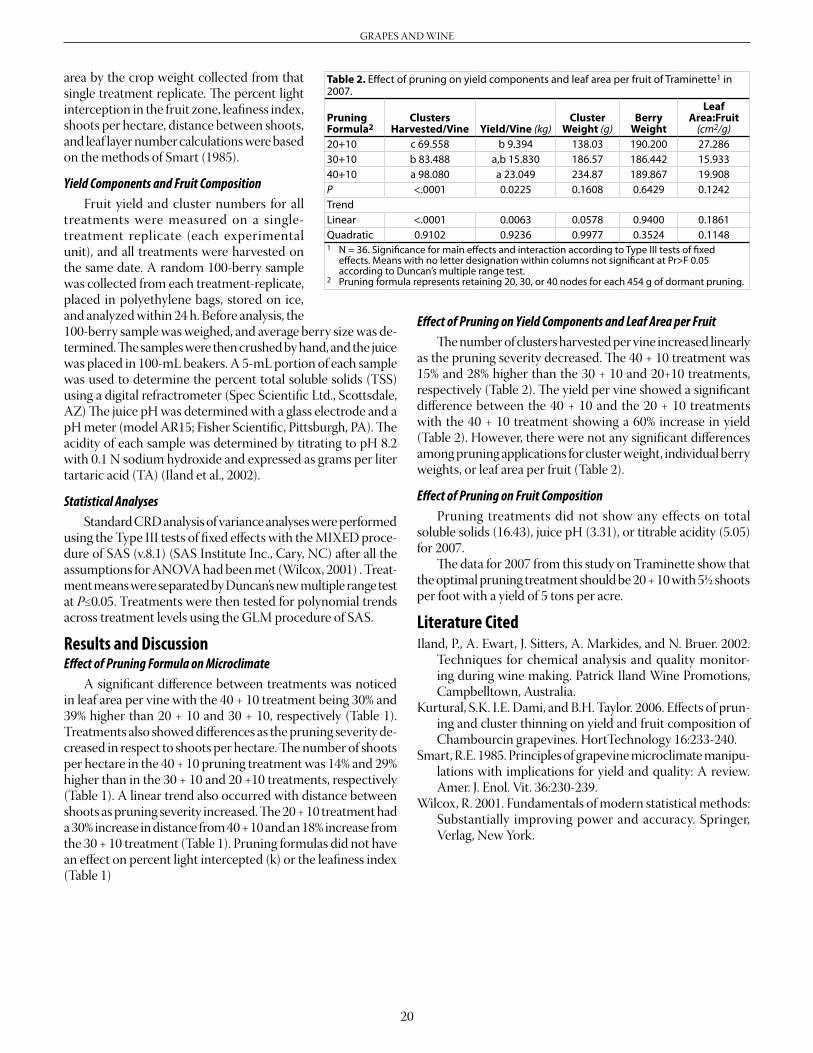
Table 2. Fruit composition of cultivars tested in 2007 at the UKREC trial at UKREC, Princeton, Ky.
Table 1. Vine size, crop load, and yield components of cultivars at the UKREC trial at UKREC, Princeton, Ky.
Cultivar
PruningWeight/ Vine1
(lb)Crop
Load2Clusters
HarvestedYield3
(T/A)Vidal Blanc 2.5cd 8.2a 119a 6.4aNiagara 2.7cd 6.4ab 111ab 5.5aChardonnay 3.2bc 6.7ab 30d 1.2cdTraminette 4.0ab 1.8d 9d 0.2ePinot Noir 4.0ab 2.2d 22d 0.5deCabernet Franc 4.5a 2.7dc 61c 1.6cChambourcin 1.5d 4.7bc 95ab 3.0bNorton 2.2cd 3.6cd 83bc 1.5bp 0.0001 0.0001 0.0001 0.00011 Pruning weight per vine in response to 2006 crop level.2 Crop load: Crop yield in 2006/Pruning weight in 2006 (lb/lb).3 T/A: Yield in tons per acre assuming 340 grapevines per acre in 2007.
Introduction There is increasing interest in growing grapes for wine pro-duction in Kentucky. Grapes have the potential to generate a high per acre income on upland sites. Kentucky grape growers need varieties that are adapted to Kentucky’s varied climates and are capable of sufficiently yielding high-quality grapes. There are four types of wine grapes grown in the United States: American (Vitis labrusca), Muscadine (Vitis rotundifo-lia), European (Vitis vinifera), and American-French hybrids (Vitis labrusca x V. vinifera). Generally, Muscadine and Euro-pean grapes are not adapted to Kentucky’s environment. On the other hand, American grapes grow well, but the wine is usually not up to par with European wines. Many American-French hybrids grow well, and wine quality is intermediate between that of the American and French parents. The majority of the wine from Europe and the West Coast of the United States is made from European grapes. The objectives of this project are to evaluate wine grape cultivars grown in different regions of the United States and to establish a baseline of performance by which other wine grape cultivars may be compared.
Material and Methods Eight cultivars were planted in the spring of 2000 at the University of Kentucky Research and Education Center in Princeton, Kentucky. These included two American cultivars (Niagara and Norton), two American-French hybrids, (Cham-bourcin and Vidal Blanc), one recently released interspecific hybrid (Traminette), and three vinifera selections (Cabernet Franc, Pinot Noir, and Chardonnay). The planting was estab-lished in an area previously used for a high-density apple plant-ing. Consequently, rows were set at 16 ft apart in order to use the end posts left from the apple planting. Vines were set at 8 ft spacing within rows. Vines were grown with two trunks and tied to 5-ft bamboo canes during the first year. During the sec-ond year, vines were trained to a high bilateral-cordon system. The planting was set up with trickle irrigation and a 4-ft wide herbicide strip beneath the vines with mowed sod alleyways. During the spring of 2002, the vinifera cultivars were converted to the vertical shoot positioning system (VSP). This system typically conforms more appropriately to the vertical growth habit of vinifera cultivars. The trellis was changed to accommodate both training systems in the spring of 2003. The experimental design is a randomized block design with six replications. In this paper, we report results from the 2006 and 2007 years. Pruning (2006) and yield data were collected for each vine. Cluster weight, berry size and weight, total soluble solids, juice pH, and titratable acidity were measured for each cultivar. Crop load for each cultivar was calculated by dividing yield per vine by the pruning weight and is reported for the 2006 year.
Results and Discussion The vine size measured in response to 2006 crop levels indicated that Cabernet Franc, Pinot Noir, Traminette, Nor-ton, and Chardonnay have too much area allocated to them. This was again evident when crop load of the cultivars tested was measured. A crop load of 5 to 8 is considered acceptable for grapevine balance, but Traminette, Pinot Noir, and Caber-net Franc have crop load values of less than 5 (Table 1). This indicates an undercropping situation forcing these cultivars into vegetative growth cycles, hence creating mutual shading within the fruit zones of the canopies, respectively. The cultivar Vidal Blanc was the best yielding cultivar in 2007 (Table 1). It was minimally affected by the advective freeze conditions en-countered in early April 2007. Niagara and Chambourcin were also minimally affected by the advective freeze; however, their yields were somewhat less than commercially accepted values due to the less-than-ideal number of vines per acre (Table 1). Traminette, Pinot Noir, and Chardonnay were most affected by the advective freeze in 2007 as evidenced by the number of clusters harvested in this year (Table 1) and reported yields.
19
GRAPES AND WINE
Fruit composition values measured in 2007 (Table 2) displayed the effects of the prolonged drought witnessed in addition to the freeze damage in this growing season. Gener-ally, the total soluble solids measured in the juice were accept-able for Norton, Chardonnay, Cabernet Franc, Pinot Noir, and Traminette. [However, the juice pH and titratable acidity
measured in the must for these cultivars indicated the effects ofthedroughtcoupledwiththehigher-than-normalday/nighttemperatures in this year (Table 2).] Fruit composition values were acceptable only for Vidal Blanc in 2007 with a total soluble solids percentage of 18.1, juice pH of 3.5, and a titratable acidity of5.2g/L.
Effect of Pruning Formula on Yield and Fruit Composition of Traminette Grapevines
S. Brandon O’Daniel, Patsy E. Wilson, Y.A. Karatus, and S. Kaan Kurtural, Department of Horticulture
Introduction Traminette is a Gewurztraminer hybrid that produces an excellent white wine with the proper balances of sugar, acid, and pH. Traminette is well adapted to climate and soil conditions found in the midwest-ern United States and shows better signs of winterhardiness than its Gewurztraminer parent. This, along with better productivity and moder-ate resistance to powdery mildew, has led to a need to better understand this vine’s canopy structure and crop-ping level.
Materials and Methods This study was conducted on a commercial vineyard in Lexington, Kentucky, with Maury silt loam soils. The study used nonirrigated own-rooted Traminette that was planted in 2001. The vines are trained on a 1.8 m high bilateral-cordon with a spacing of 2.4 x 4 m (vine x row) and were spur-pruned. Nitrogen was applied annually at a rate of 34 kg per hectare. The experiment used a 3 x 12 (pruning for-mula x replication) arrangement of treatments in a completely randomized design.
Pruning Treatments Previous year’s (2006) canes were pruned to five-node canes to an upper limit of 65 nodes per vine. The prunings were weighed (Table 1), and the number of nodes to be left on the vine in 2007 was then determined by the weight of the cane prunings removed. The buds at these nodes are referred to hereafter as count-buds. The three levels of pruning severity selected were (20 + 10), (30 + 10), and (40 + 10). Level numbers refer to number of buds left for the initial 1 pound of prunings, plus number of buds retained for each additional pound of prunings.
Table 1. Effect of pruning formula on the microclimate of Traminette1 in 2007.
Pruning Formula2 k3
Leaf Area per Vine4 (m2)
γ5
(cm2/cm)Shoots per
Hectare6
Distance between
Shoots7 (cm)Leaf Layer Number8
20+10 8.1058 b 23.799 50.978 c 45827 a 5.5775 b 8.04830+10 7.6650 b 20.521 35.601 b 55004 b 4.5608 b 6.81840+10 8.3600 a 33.231 54.024 a 64618 c 3.8883 a 12.138P 0.4263 0.0265 0.1372 <.0001 <.0001 0.0241Trend9
Linear 0.6356 0.0498 0.7533 <.0001 <.0001 0.0413Quadratic 0.2261 0.0545 0.0505 0.9105 0.9105 0.05821 N = 36. Significance for main effects and interaction according to Type III tests of fixed effects. Means
with no letter designation within columns not significant at Pr>F 0.05 according to Duncan’s multiple range test.
2 Pruning formula represents retaining 20, 30, or 40 nodes for each 454 g of dormant pruning.3 k = (Percent light intercepted): [(PPFD intercepted in fruit zone / PPFD ambient) x 100]. 4 Leaf area per vine = leaf area per shoot x number of shoots per vine.5 γ = (leafiness index): leaf area per shoot/shoot length.6 Shoots per hectare = total shoots per vine x vines per hectare.7 Distance between shoots = 1,000,000/row width (4 meters) x shoots per hectare. 8 Leaf layer number = γ x 0.866/distance between shoots.9 Trend analyses carried to the quadratic level using single degree of freedom planned orthogonal
contrasts.
Shoot Counts and Pruning Weights At bud burst, total shoots and nodes that did not produce a shoot were counted. Count shoots (borne from count-buds retained at pruning > 5 mm distal to the base of the cane), non-count shoots (borne from basal buds < 5 mm distal to the base of the cane or on wood older than one year), and total shoots (count + non-count shoots) retained per vine were measured. During the growing season, shoots were vertically positioned downward, every 14 days to reduce intra-vine shading. No leaf removal was conducted in the fruit zone.
Canopy Microclimate One count-shoot per vine was harvested 10 weeks post-bloom. Count-shoots were placed in a sealed plastic bag and kept in cold storage until measured. The shoots were then sepa-rated into main and lateral axes. Leaf area of individual leaves was measured using a LI-3000 (Li-Cor, Inc., Lincoln, NE) leaf area meter. The number of leaves measured for each axis was counted. The total leaf area for each shoot was calculated by add-ing the areas for the main and the lateral axis. The total canopy leaf area was calculated by multiplying the total shoot number for that treatment replicate by the total leaf area per shoot. The leaf area:fruit (cm2/g)wascalculatedbydividingthecanopyleaf
20
GRAPES AND WINE
Table 2. Effect of pruning on yield components and leaf area per fruit of Traminette1 in 2007.
Pruning Formula2
Clusters Harvested/Vine Yield/Vine (kg)
Cluster Weight (g)
Berry Weight
Leaf Area:Fruit
(cm2/g)20+10 c 69.558 b 9.394 138.03 190.200 27.28630+10 b 83.488 a,b 15.830 186.57 186.442 15.93340+10 a 98.080 a 23.049 234.87 189.867 19.908P <.0001 0.0225 0.1608 0.6429 0.1242TrendLinear <.0001 0.0063 0.0578 0.9400 0.1861Quadratic 0.9102 0.9236 0.9977 0.3524 0.11481 N = 36. Significance for main effects and interaction according to Type III tests of fixed
effects. Means with no letter designation within columns not significant at Pr>F 0.05 according to Duncan’s multiple range test.
2 Pruning formula represents retaining 20, 30, or 40 nodes for each 454 g of dormant pruning.
area by the crop weight collected from that single treatment replicate. The percent light interception in the fruit zone, leafiness index, shoots per hectare, distance between shoots, and leaf layer number calculations were based on the methods of Smart (1985).
Yield Components and Fruit Composition Fruit yield and cluster numbers for all treatments were measured on a single-treatment replicate (each experimental unit), and all treatments were harvested on the same date. A random 100-berry sample was collected from each treatment-replicate, placed in polyethylene bags, stored on ice, and analyzed within 24 h. Before analysis, the 100-berry sample was weighed, and average berry size was de-termined. The samples were then crushed by hand, and the juice was placed in 100-mL beakers. A 5-mL portion of each sample was used to determine the percent total soluble solids (TSS) using a digital refractrometer (Spec Scientific Ltd., Scottsdale, AZ) The juice pH was determined with a glass electrode and a pH meter (model AR15; Fisher Scientific, Pittsburgh, PA). The acidity of each sample was determined by titrating to pH 8.2 with 0.1 N sodium hydroxide and expressed as grams per liter tartaric acid (TA) (Iland et al., 2002).
Statistical Analyses Standard CRD analysis of variance analyses were performed using the Type III tests of fixed effects with the MIXED proce-dure of SAS (v.8.1) (SAS Institute Inc., Cary, NC) after all the assumptions for ANOVA had been met (Wilcox, 2001) . Treat-ment means were separated by Duncan’s new multiple range test at P≤0.05. Treatments were then tested for polynomial trends across treatment levels using the GLM procedure of SAS.
Results and DiscussionEffect of Pruning Formula on Microclimate A significant difference between treatments was noticed in leaf area per vine with the 40 + 10 treatment being 30% and 39% higher than 20 + 10 and 30 + 10, respectively (Table 1). Treatments also showed differences as the pruning severity de-creased in respect to shoots per hectare. The number of shoots per hectare in the 40 + 10 pruning treatment was 14% and 29% higher than in the 30 + 10 and 20 +10 treatments, respectively (Table 1). A linear trend also occurred with distance between shoots as pruning severity increased. The 20 + 10 treatment had a 30% increase in distance from 40 + 10 and an 18% increase from the 30 + 10 treatment (Table 1). Pruning formulas did not have an effect on percent light intercepted (k) or the leafiness index (Table 1)
Effect of Pruning on Yield Components and Leaf Area per Fruit The number of clusters harvested per vine increased linearly as the pruning severity decreased. The 40 + 10 treatment was 15% and 28% higher than the 30 + 10 and 20+10 treatments, respectively (Table 2). The yield per vine showed a significant difference between the 40 + 10 and the 20 + 10 treatments with the 40 + 10 treatment showing a 60% increase in yield (Table 2). However, there were not any significant differences among pruning applications for cluster weight, individual berry weights, or leaf area per fruit (Table 2).
Effect of Pruning on Fruit Composition Pruning treatments did not show any effects on total soluble solids (16.43), juice pH (3.31), or titrable acidity (5.05) for 2007. The data for 2007 from this study on Traminette show that the optimal pruning treatment should be 20 + 10 with 5½ shoots per foot with a yield of 5 tons per acre.
Literature CitedIland, P., A. Ewart, J. Sitters, A. Markides, and N. Bruer. 2002.
Techniques for chemical analysis and quality monitor-ing during wine making. Patrick Iland Wine Promotions, Campbelltown, Australia.
Kurtural, S.K. I.E. Dami, and B.H. Taylor. 2006. Effects of prun-ing and cluster thinning on yield and fruit composition of Chambourcin grapevines. HortTechnology 16:233-240.
Smart, R.E. 1985. Principles of grapevine microclimate manipu-lations with implications for yield and quality: A review. Amer. J. Enol. Vit. 36:230-239.
Wilcox, R. 2001. Fundamentals of modern statistical methods: Substantially improving power and accuracy. Springer, Verlag, New York.
21
GRAPES AND WINE
Effect of Training Systems on Vine Size, Yield Components, and Fruit Composition of European Grapevines
S. K. Kurtural, J. Strang, C. Smigell, Y.A. Karatas, P.E. Wilson, and S.B. O’Daniel, Department of Horticulture
Introduction Kentucky growers have planted extensive grape acreage for wine production over the last nine years. Roughly 21% of these grapes are vinifera, or European, cultivars that are prone to win-ter freeze and late spring frost damages. Additionally, frequent exposure to critical winter temperatures makes the European grapevines susceptible to crown gall infection (a bacterial dis-ease, Agrobacterium vitis), which begins at wounds caused by freeze-induced trunk splitting. Crown gall can severely weaken or kill the vines. The objectives of this study were to compare survival, yield, and fruit quality between the vertically shoot positioned (VSP) and fan-trained grapevine cultivars.
Materials and Methods One-year-old, dormant, bare root grapevines of the vinifera cultivars Cabernet Franc clone #332 (fairly hardy), Chardon-nay clone #76 (moderately hardy), Shiraz (least hardy), and the French-American hybrid Vidal Blanc (very hardy) were planted in the spring of 2002 at the University of Kentucky Horticultural Research Farm in Lexington on Maury silt-loam soil. All cultivars were grafted onto the C-3309 rootstock except one treatment of Vidal Blanc that was on its own roots. Vines were spaced 8 ft within the row and 12 ft (454 plants.acre-1) between rows in a randomized block factorial design with six replications. Half the grapevines were trained using the VSP system, in which vines are developed with two trunks, each becoming a cordon on the lowest wire (38 inches above the vineyard floor). From these cordons, shoots are trained vertically between two sets of catch wires (spaced 12 inches above the training wire). The remaining grapevines were fan-trained, which consists of up to six canes radiating out from the vine base or graft union in a fan pattern and tied to the trellis. In 2005, metal trellis post extensions were installed to increase leaf area, bringing the exposed height of the canopy to 5 ft. Vines were watered as needed until established, and weeds were controlled in a 3-ft wide herbicide strip down the row be-neath the vines. Mowed sod middles were maintained between rows. Graft unions were covered with soil annually in late fall to protect unions from freeze injury. Vines were trained during the first two seasons and balance pruned in 2004 and 2005 to adjust fruit load to vine size. In subsequent years, all vines were pruned to 40 nodes per vine to remove the confounding effects of crop level on the grapevines. Additional cluster and shoot thinning were performed on vines that had excessive crops and vine size, respectively. Insecticide, fungicide, and herbicide applications were made in accordance with the Midwest Grape and Small Fruit Spray Guide (ID-94).
Vines were fruited for the first time in 2005. Here we report results from the 2006 and 2007 growing seasons. Vine size and crop load for the 2006 season and shoot density, yield, cluster weight, berry weight, total soluble solids (TSS), juice pH, and titratable acids (TA) for 2007 were measured.
Results and Discussion Vine size was not affected by the training system treatments in 2006 (Table 1). The vine sizes of the cultivars tested were also not affected in 2006. The mean of the vine sizes for all cultivars was 0.53 lb per ft of canopy in 2006, indicating the vines were in balance. Crop load (ratio of yield to vine size) was not af-fected by the training systems in 2006 (Table 1). However, the five cultivars tested carried varying crop loads on them. The VidalBlanc/C3309andtheVidalBlanconitsownrootshadthe highest crop loads in 2006. All crop loads were within the recommended ranges for cultivars tested. The number of count shoots retained was 12% higher for the fan system-trained grapevines than for the VSP-trained ones. Vidal Blanc, whether on rootstock or not, had significantly more count shoots retained than did any of the European cultivars (Table 1). On the other hand, the number of non-count shoots retained in the VSP-trained grapevines, regardless of cultivar, was 31% higher than in the fan-trained grapevines. Due to the severe freeze of April 2007, the amount of non-count shoots retained was higher in the European cultivars, in order to at-tain 40 nodes per vine (Table 1). Still, the number of non-count shoots removed during shoot thinning was 22% higher in the fan system-trained grapevines compared to the VSP-trained vines. The total number of shoots retained per vine was not affected by the training system used. However, the cultivars tested had different total number of shoots retained in 2007 when measured at berry touch, post-shoot thinning. The Vidal Blanc vines tended to have the most total shoots retained, due to the many fruitful shoots arising from non-count positions (Table 1). The total number of clusters per vine was not affected by the training system used (Table 2). However, the cluster num-ber varied by cultivar. As expected, the hybrid (Vidal Blanc) grapevines carried more clusters than the European grapevines. Shiraz grapevines had the lowest number of marketable clusters. The number of marketable clusters per vine was 10% higher for the fan system-trained vines in 2007 than for the VSP-trained vines (Table 2). The Vidal Blanc vines had the highest number of marketable clusters compared to the European cultivars. The number of culled clusters per vine was not affected by the train-ing system treatments (Table 2). Cabernet Franc had the highest number of culled clusters per vine in 2007. The Vidal Blanc, whether on its own roots or on the 3309 rootstock, had the highest yield in 2007. Chardonnay and Shiraz had the smallest yields (Table 2). Cluster weight was 7% higher for VSP-trained
22
GRAPES AND WINE
grapevines compared to the fan-trained grapevines. The TSS levels were not affected by the training sys-tem used (Table 3). However, among the cultivars tested, Shiraz had the highest TSS and own-rooted Vidal Blanc had the lowest. The juice pH was not affected by the training sys-tem used (Table 3). However, Shiraz had the highest juice pH at harvest, and Vidal Blanc on its own roots and on the 3309 rootstock had the lowest. The TA in the must was not affect-ed by the training system used (Table 3). However, Vidal Blanc on its own roots and on the 3309 rootstock had the high-est TA, while Chardonnay had the lowest. The berry weight was 3% larger in VSP-trained grapevines when compared to fan-trained grapevines in 2007 (Table 3). In 2007, due to the advec-tive freeze event in the first week of April, the grapevines of all five cultivars suffered tissue damage. Therefore, the num-ber of shoots retained on the vines was adjusted by retaining some non-count shoots. This explains the lack of interaction among cultivars and training systems. Even with the damag-ing effects of the April freeze and the necessity of retaining some non-count shoots, the fan-trained grapevines needed more aggressive canopy man-agement (i.e., removal of some of the non-count shoots) than did the VSP-trained vines.
Table. 1. Effect of training system and cultivar on 2006 season’s vine size and crop load and 2007 season shoot density.
Cultivar
Vine Size per Foot of Canopy1,2
(lb/ft)
Crop Load3 (lb/lb)
Count Shoots
Retained
Non-Count Shoots
Retained
Non-Count Shoots
Removed
Total Shoots
per VineChardonnay 0.44 5.9 b 19 c 18 a 24 a 37 bcCabernet Franc 0.59 5.9 b 27 b 18 a 29 a 45 abShiraz 0.67 4.2 b 18c 17 a 17 b 36 cVidal Blanc/own roots 0.54 8.2 b 37 a 8 b 15 b 46 aVidal Blanc/C3309 0.40 16 a 35 a 11 ab 15 b 49 ap< 0.4302 0.0077 0.0001 0.0215 0.0001 0.0084Training SystemFan 0.52 9.4 29 a 13 22 a 42VSP 0.54 6.5 26 b 17 18 b 42p< 0.4302 0.1470 0.0267 0.0570 0.0271 0.8051Cultivar x Training System 0.3088 0.2827 0.1129 0.2721 0.1244 0.31591 Means within a column followed by the same letter are not significantly different (Duncan’s multiple range
test, Pr>F 0.05).2 Vine size is the amount (in lb) of prunings per horizontal foot of canopy.3 Crop load is the ratio of a vine’s yield for one season to the dormant pruning weight the following season.
Table 2. Effect of training system and cultivar on yield components, 2007.
Cultivar/Harvest Date
Total Clusters/
Vine1
Marketable Clusters/
Vine
CulledClusters/
Vine2
Marketable Weight/Vine
(lb)Yield3
(tons/acre)
Cluster Weight
(g)Chardonnay/8 Sep 45 c 43 b 2 d 9.3 c 2.1 c 98.0 cCabernet Franc/27 Sep 67 b 49 b 18 a 16.5 b 3.7 b 155.5 bShiraz/27 Sep 39 c 30 c 9 bc 10.2 c 2.3 c 155.3 bVidal Blanc—own/6 Oct 78 a 73 a 5 cd 29.1 a 6.6 a 179.2 aVidal Blanc—C3309/6 Oct 81 a 71 a 11 b 26.6 a 6.1 a 171.7 abp< 0.0001 0.0001 0.0001 0.0001 0.0001 0.0001Training SystemFan 64 56 a 7 18.8 4.3 146.7 bVSP 59 50 b 10 17.9 4.1 157.9 ap< 0.1584 0.0139 0.0934 0.3884 0.3884 0.0300Cultivar x Training System 0.2382 0.1241 0.9537 0.0873 0.0873 0.83611 Means within a column followed by the same letter are not significantly different (Duncan’s multiple range
test, Pr>F 0.05).2 Clusters that displayed >30% visual damage by fungal infection, bird damage, sunburn.3 Based on 454 vines/acre.
Table 3. Effect of training system and cultivar on fruit composition.
CultivarTotal
Clusters1 TSS2 Juice pH TA3Berry
Weight (g)Chardonnay 45 c 18.8 b 3.33 c 3.8 d 1.71 cCabernet Franc 67 b 19.1 b 3.53 b 5.5 c 1.66 cShiraz 39 c 19.9 a 3.72 a 5.3 c 2.18 aVidal Blanc/own roots 78 a 17.6 c 3.03 e 8.3 a 1.95 bVidal Blanc/C3309 81 a 18.7 b 3.15 d 7.7 v 1.95 bp< 0.0001 0.0001 0.0001 0.0001 0.0001Training SystemFan 64 18.9 3.35 6.1 1.87 bVSP 59 18.7 3.35 6.1 1.93 ap< 0.1584 0.2930 0.4016 0.9093 0.0392Cultivar x Training System 0.2382 0.8190 0.1497 0.5830 0.41001 Means within a column followed by the same letter are not significantly different (Duncan’s
multiple range test, Pr>F 0.05).2 TSS = total soluble solids measured as oBrix in juice.3 TA = titratable acidity measured as grams of tartaric acid in liter of juice.
23
GRAPES AND WINE
Effect of Pruning and Cluster Thinning on Crop Load and Coldhardiness of Vidal Blanc Grapevines
Patsy E. Wilson, Douglas Archbold, and S. Kaan Kurtural, Department of Horticulture
Introduction Understanding grapevine balance, the balance between reproductive and vegetative growth, in-cludes defining the crop level and crop load of the grapevine based on canopy management practices. Canopy management of the grapevine includes re-taining a set number of shoots per length of canopy, positioning the shoots within the canopy, thinning the infructescence, skirting or hedging the shoots, and removing the leaves around the clusters. Crop level is defined as the number of clusters retained per shoot, per unit of dormant cane pruning weight, or per unit of canopy length (Naor et al., 2002). Crop load is the ratio of crop yield to dormant cane pruning weight in one season (Ravaz, 1911). Proper grapevine canopy management will ensure balanced crop loads. This allows the grapevine to ripen more fruit without adversely affecting fruit composition, primary bud coldhardiness, or carbohydrate balance in the vine. There is insufficient knowledge for cropping levels and crop load of French-American hybrids in Kentucky. The basal buds of French-American hybrids tend to be fruitful; thus, cultivars such as Vidal Blanc tend to overcrop if not managed with the balanced cropping approach. Overcropping results in undesirable fruit composition in the current year and inappropriate levels of carbohydrate supply to the roots, shoots, and trunk; it also adversely affects spring growth by reducing primary bud coldhardi-ness. The goals of this study are to investigate the effect of pruning and cluster thinning on crop load and coldhardiness of Vidal Blanc grapevines under the long and warm growing season of Kentucky. The specific objectives are to determine the effects of crop load on fruit composition, periderm formation, dormant cane weights, and primary bud coldhardiness.
Materials and MethodsVineyard Site and Plant Material This study was conducted at a commercial vineyard located in central Kentucky (lat. 37º54’ N, long. 84º26’W). The site rests at an absolute elevation of 1,030 ft, and the soil type is Maury silt loam (a fine, mixed, semiactive, mesic, typic Paleudalfs). Own-rooted Vidal Blanc vines were planted in 2001 at 545 vines/acreatan8×12ft(vine×row)spacing.Vineswerespur-pruned and trained to a 6-ft single high wire bilateral-cordon in a north-south facing arrangement for maximum light intercep-tion. Nitrogen was applied annually at 30 lb.A-1, and vines were notirrigated.Experimentalsetupconsistedofa3×3factorial
arrangement in a completely randomized block design with four vines per replication and three vines designated as an experimental unit.
Pruning Treatments Canes from the previous year (2005) were pruned to five-node canes with an upper limit of 65 nodes per vine. Dormant prunings were weighed, and final node counts per vine were determined by dormant pruning weights and pruning severity level. Buds retained at these nodes are referred to as count-buds, as opposed to non-count, or basal, buds. Three levels of prun-ing severity were applied: 20 + 10, 30 + 10, and 40 + 10. These levels refer to the number of buds retained per initial pound of dormant prunings plus the number of buds retained for each additional pound of prunings (e.g., 20 buds for the initial pound of prunings and 10 buds for each additional pound of prunings).
Table 1. Effect of pruning formula and cluster thinning in 2006 on pruning weights, crop load, and leaf area to fruit ratio of Vidal Blanc grapevines.1
1 cluster·shoot-1 20.5ab 19.0 0.3141ab 7.69b 32.21a2 cluster·shoot-1 22.6a 18.9 0.3297a 10.86b 23.36ab2+ cluster·shoot-1 16.2b 16.8 0.2618b 16.25a 17.07bp< 0.0302 0.4946 0.0297 0.0045 0.0163TrendLinear 0.3605 0.9241 0.5424 0.1698 0.0441Quadratic 0.0128 0.2404 0.0100 0.0012 0.0326Pruning × Thinning 0.1504 0.4946 0.0840 0.8144 0.8912 1 n = 36. Significance for main effects and interaction according to Type III tests of
fixed effects. Means with no letter designation within columns not significant at Pr>F 0.05 according to Duncan’s multiple range test.
2 Pruning formula represents retaining 20, 30, or 40 nodes for each pound of dormant pruning.
3 Mature cane weight measured on canes displaying >10-in. periderm formation.4 Die-back cane weight measured on canes displaying < 10-in. periderm formation.5 Vine size per foot of row = dormant pruning weight (lb) per length of canopy (ft)
measured during treatment application in 2007 in response to 2006 growing season.6 Crop load: lb yield/vine ÷ lb pruning wt/vine.7 Leaf area: fruit = leaf area (cm2) per vine ÷ g yield per vine.8 Trend analyses carried to the quadratic level using single degree of freedom planned
orthogonal contrasts.9 Cluster thinning treatments represent post-fruit set cluster thinning at Eichorn-
Lorenz scale 31 where 1 cluster, 2 clusters, and 2+ clusters per shoot were retained.
24
GRAPES AND WINE
Cluster Thinning Treatments In 2006, three cluster thinning severity levels were applied two to three weeks post-bloom (2 to 3 mm diameter berry size). Cluster thinning treatments were then adjusted post-fruit set at Eichorn-Lorenz scale 31 where 1 cluster per shoot (thinned to basal cluster), 2 clusters per shoot, or 2+ clusters per shoot were retained.
Berry Sampling and Fruit Composition Fruit yield and cluster numbers for all treatments in 2006 were measured on a single treatment replicate (each experi-mental unit), and all treatments were harvested on the same date. A random 100-berry sample was collected from each treatment-replicate, placed in polyethylene bags, stored on ice, and analyzed within 24 hours. Before analysis, the 100-berry sample was weighed, and average berry weight was determined. The samples were then crushed by hand, and the juice was placed in 250 mL beakers. A 5 mL portion of each sample was used to determine the percent total soluble solids (TSS) using a digital refractometer (Spec Scientific Ltd., Scottsdale, AZ). The juice pH was determined with a glass electrode and a pH meter (model AR15; Fisher Scientific, Pittsburgh, PA). The titratable acidity (TA) of each sample was determined by titrating to pH 8.2 with 0.1 N sodium hydroxide and expressed as grams per liter of tartaric acid (Iland et al., 2002).
Crop Load and Leaf Area to Fruit Ratio Crop load was calculated by dividing the yield per vine in 2006 by the dormant cane pruning weights measured during pruning the following spring. The leaf area to fruit ratio was calculated by dividing the leaf area per vine by the yield per vine.
Periderm Browning and Primary Bud Coldhardiness In 2006, periderm browning was measured on 26 September (one week post-harvest) and 8 November (after the occurrence of killing frost). The ratio of mature nodes to total nodes of 10 canes for each treatment was calculated for percent periderm browning per cane. Primary bud coldhardiness was determined by harvesting dormant canes on 23 January 2007. Twenty-seven nodes from each treatment were harvested and cut into three-node sec-tions. Three replications from each treatment were subjected to simulated freeze tests at temperatures of 0° to -40°C in 2.5°C/hincrements with a 60 min exposure period for each increment. Buds were then thawed for 48 h at 4°C, sectioned free-hand, and oxidative browning was measured.
Statistical Analysis Standard, completely randomized design analyses of vari-ance (ANOVA) were performed using the Type III tests of fixed effects with the MIXED procedure of SAS (v.8.1) (SAS Institute Inc., Cary, NC), after all the assumptions for ANOVA had been met (Wilcox, 2001). Treatment means were then tested for polynomial trends across treatment levels using the GLM procedure of SAS.
Table 3. Effect of crop load and leaf area-to-fruit ratio in 2006 on cluster architecture, fruit composition, and canopy variables of Vidal Blanc grapevine.1
1 n = 36. Data presented is first-year data from a two-year study.2 Crop load: lb yield per vine ÷ lb pruning wt per vine.3 Leaf area:fruit = leaf area (cm2) per vine ÷ g yield per vine.4 Mature cane wt measured on canes displaying >25 cm periderm
formation.5 Die-back cane wt measured on canes displaying <25 cm periderm
formation.6 Number of mature nodes per shoot measured on nodes if the entire
node, bud, and basipetal internodes had turned from green to brown after occurrence of killing frost.
Table 2. Effect of pruning formula and cluster thinning in 2006 on midwinter primary bud coldhardiness and mature node count of Vidal Blanc grapevines.1
Linear 0.2153 0.5764Quadratic 0.9570 0.2675Cluster Thinning6
1 cluster·shoot-1 -13.60 63.542 cluster·shoot-1 -14.11 63.762+ cluster·shoot-1 -10.07 61.62p< 0.0939 0.9328TrendLinear 0.0789 0.9717Quadratic 0.1853 0.7126Pruning × Thinning 0.6325 0.58121 n = 36. Data presented is first-year data from a two-year study.2 Pruning formula represents retaining 20, 30, or 40 nodes for each
pound of dormant pruning.3 LT50 calculated based on temperature required to kill 50% of buds
using a nonlinear regression model.4 Measured on nodes if the entire node, bud, and basipetal internodes
had turned from green to brown.5 Trend analyses carried to the quadratic level using single degree of
freedom planned orthogonal contrasts.6 Cluster thinning treatments represent post-fruit set cluster thinning at
Eichorn-Lorenz scale 31 where 1 cluster, 2 clusters, and 2+ clusters per shoot were retained.
25
GRAPES AND WINE
Results and DiscussionEffect of Pruning Formula and Cluster Thinning on Vine Size, Crop Load, and Leaf Area to Fruit Ratio Pruning formula treatments in 2006 did not affect vine size, crop load, or leaf area to fruit ratio (Table 1). Mature pruning weights in response to the cluster thinning treatments were 10% and28%higherforthetwoclusters/shoottreatmentcomparedto the 1 and 2+ clusters per shoot treatments in 2006, respec-tively (Table 1), fitting a quadratic trend. The die-back pruning weight was not affected by the cluster thinning treatments in 2006. Vine size per meter of row (vigor) of 1 cluster and 2 clusters/shoottreatmentswere20%higherthanthe2+clustersper shoot treatment in 2006 indicating excessive crop on the 2+ clusters per shoot treatment (Table 1). Crop load in 2006 increased linearly as the severity of cluster thinning decreased (Table1).Thecroploadof2+clusters/shootand2cluster/shoottreatmentswere53%and30%higherthanthe1cluster/shoottreatment, respectively, in 2006 (Table 1). The leaf area to shoot ratioof1cluster/shootwas28%and47%higherin2006thanthe2clusters/shootand2+clustersper shoot, respectively,indicating that there was not enough fruit in 2006 in relation totheamountofleafareaonthe1cluster/shoottreatment.
Effect of Pruning Formula and Cluster Thinning on Periderm Browning and Primary Bud Coldhardiness Pruning formula treatments did not affect the primary bud coldhardiness or the percentage of mature nodes on Vidal Blanc grapevines in 2006 (Table 2). However, the cluster thinning treatments in 2006 displayed a weak linear trend on the primary bud coldhardiness of Vidal Blanc grapevines. As the severity of cluster thinning increased, there was a slight tendency of the primary bud coldhardiness to increase (Table 2).
Effect of Crop Load and Leaf Area to Fruit Ratio on Cluster Architecture, Fruit Composition, and Vine Size In 2006, there was a negative relationship between crop load and cluster weight of Vidal Blanc (Table 3). As crop load increased, the cluster weight decreased linearly. A similar relationship was not evident between leaf area to fruit ratio and cluster weight in 2006 (Table 3). In 2006, berry weight was not affected by the crop load (Table 3). However, berry weight increased linearly with the increase in the leaf area to fruit ratio (Table 3). The number of berries per cluster decreased linearly with the decrease in crop load and increased as with the in-crease in the leaf area to fruit ratio (Table 3). Fruit composition was not affected by crop load or leaf area to fruit ratio in 2006 (Table 3).
Figure 1. Relationship between percent mature nodes per shoot after occurrence of killing frost and LT50 of primary buds in midwinter in response to canopy management of Vidal Blanc grapevines in 2006.
Mature pruning weight increased linearly with the de-crease in crop load (Table 3), and the die-back pruning weight increased linearly with the increase in crop load in 2006 (Table 3). Number of mature nodes per shoot was not affected by crop load in 2006. The leaf area to fruit ratio in 2006 did not affect pruning weights or the number of mature nodes per shoot (Table 3).
Effect of Carbohydrate Balance on Primary Bud Coldhardiness The amount of the mature nodes on canes after the oc-currence of killing frost indicates how well the grapevine can allocate carbohydrate resources to non-fruiting portions of the grapevine such as shoots and roots at a given crop level and crop load. In 2006, as the percent of mature nodes per shoot increased, the primary bud coldhardiness of Vidal Blanc increased (Figure 1).
Literature CitedNaor, A., Y. Gal., and B. Bravado. 2002. Shoot and cluster thin-
ning influences vegetative growth, fruit yield, and wine quality of Sauvignon Blanc grapevines. J. Amer. Soc. Hort. Sci. 127:628-634.
Ravaz, M.L. 1911. L’effeuellage de la vigne. Annales d L’Ecole Nationale d’agriculture de Montpellier 11:216-244.
Wilcox, R. 2001. Fundamentals of modern statistical methods: Substantially improving power and accuracy. Springer, Verlag, New York.
26
GRAPES AND WINE
Effects of Pruning and Cluster Thinning on Microclimate, Yield, and Fruit Composition of Vidal Blanc Grapevines
Patsy E. Wilson, S.B. O’Daniel, Y.A. Karatas, and S. K. Kurtural, Department of Horticulture
Kentucky’s grape and wine industry has been growing due to increased interest from private investors and local demand. There are 48 wineries in Kentucky, of which 44 are in produc-tion (Cottrell, 2007 personal communication). Vidal Blanc is of economic importance to Kentucky and the eastern United States, comprising 25% of Kentucky’s vineyard acreage (Smigell et al., 2005.) Vidal Blanc is an inter-specific hybrid of white wine grapes and is a cross of Ugni Blanc and Rayon d’Or (Siebel 4986). Due to its winterhardiness, this cultivar is grown in regions with harsh climates. The grapefruit and pineapple aroma coupled with the high total soluble solids and desired acid levels make it desirable to winemakers. However, French-American hybrids such as Vidal Blanc have the propensity to overcrop due to high cluster numbers and fruitful secondary shoots (Pool et al., 1978.) For this reason, if growers do not practice canopy management, they tend to overcrop this cultivar, decreasing fruit and wine quality, vine vigor, vine capacity, and midwinter primary bud coldhardiness, in years following overcropping (Dami et al., 2006). There are insufficient studies, and therefore insufficient guidelines, for cropping levels and crop load of French-Ameri-can hybrids. The fruitful French-American hybrids tend to over-crop with traditional dormant pruning. Canopy management practices including balanced pruning, shoot positioning, and cluster thinning should be combined to minimize overcropping in these hybrid cultivars. Due to the long and warm growing seasons typical of Kentucky, the established guidelines for balanced pruning and cluster thinning of Vidal Blanc cannot be applied because studies were conducted in cooler regions such as Michigan and New York. For this reason, new research is necessary to produce the proper balanced cropping regime for Kentucky to improve vine balance and increase yields and fruit quality for Vidal Blanc. The goals of this study are to investigate the ability of Vidal Blanc to ripen a commercial crop without adversely affecting yield and fruit composition under the long, warm growing seasons typical of the lower midwestern United States The specific objectives are to investigate the effects of balanced pruning and cluster thinning on canopy microclimate, yield components, and fruit composition for Vidal Blanc grown in the lower midwestern United States.
Materials and Methods Vineyard Site and Plant Material This study was conducted at a commercial vineyard located in central Kentucky (lat. 37º54’ N, long. 84º26’W). The site’s ab-solute elevation is 1,030 ft, and the soil type is Maury silt loam (fine, mixed, semiactive, mesic typic Paleudalfs). Own-rooted VidalBlancgrapevineswereplantedin2001at545vines/acreatan8×12ft(vine×row)spacinginnorth-southorientation.Vines were spur-pruned and trained to a 6 ft single high wire,
bilateral-cordon. Nitrogen fertilizer was applied annually at 30 lb·A-1, and vines were not irrigated. The experimental setup consistedof3×3factorialarrangementinacompletelyran-domized block design with three vines per replication and three vines designated as an experimental unit.
Balanced Pruning Formula Treatments Canes from the previous year (2006) were pruned to five-node canes with an upper limit of 65 nodes per vine. Dormant prunings were weighed, and final node counts per vine were determined by balanced pruning formula treatments. Buds retained at these nodes are referred to as count-buds versus non-count buds. Three balanced pruning formulas were applied: 20 + 10, 30 + 10, and 40 + 10. Formulas refer to the number of buds retained per initial pound of dormant prunings plus the number of buds retained for each additional pound of prunings (e.g., 20 buds for the initial pound of prunings + 10 buds for each additional pound of prunings).
Cluster Thinning Treatments In 2007, three cluster thinning severity levels were applied two to three weeks post-bloom (2 to 3 mm diameter berry size). Cluster thinning treatments were then adjusted post-fruit set where either 1 cluster per shoot (thinned to basal cluster), 2 clusters per shoot, or 2+ clusters per shoot were retained (no cluster thinning).
Canopy Leaf Area and Microclimate In 2007, one count-shoot was harvested on 21 June (Keller et al., 2004). Shoots were placed in sealed plastic bags and kept in storage until measured. Shoots were separated into main and lateral axes. Individual leaf areas were measured using a LI-3000 (Li-Cor, Inc., Lincoln, NE) leaf area meter. The number of leaves measured for each axis was counted. The total leaf area for each shoot was calculated by adding the areas for the main and lateral axes. The canopy leaf area was calculated by multiplying the total shoot number for that treatment-replicate by the total leaf area per shoot (Keller et al., 2004). Calculations for percent light interception (k), leafiness index (γ), shoots per acre, distance between shoots, and leaf layer number (LLN) were done as described by Smart (1985) as follows: • Percentofphotosyntheticphotondensity intercepted in
fruitzonePPFD(k)= [(PPFD intercepted in fruitzone/PPFD ambient) x 100];
shoots per acre; • Leaf layernumber(LLN)=γx0.866/distancebetween
shoots.
27
GRAPES AND WINE
Yield Components A single treatment-replicate vine from each experimental unit in each treatment group was harvested on 23 August 2007. Total yield was weighed using an electronic scale. Clusters dis-playing > 30% damage were culled and weighed separately. Clusters per vine were counted, and cluster weight was calculated by dividing total yield by total clusters harvested.
Berry Sampling and Fruit Composition A random 100-berry sample was collected from each treatment-replicate during harvest. These samples were used to determine total soluble solids (TSS), titratable acidity (TA), pH, and berry weight. Berry samples were placed in polyethylene bags, stored on ice, and analyzed within 24 hours. Before analysis, the 100-berry sample was weighed, and average berry weight was determined. The samples were then crushed by hand, and the juice was placed in 250 mL beakers. A 5 mL portion of each sample was used to determine the percent TSS using a hand-held temperature-compensated refractometer. The juice pH was determined with a glass electrode and a pH meter (accumet XL15; Fisher Scientific, Pittsburgh, PA). The TA of each sample was determined by titrating to pH 8.2 with 0.1 N sodium hydroxide and expressed as grams per liter tartaric acid (Iland et al., 2002).
Statistical Analyses Standard completely randomized design analysis of vari-ance analyses (ANOVA) was performed using the General Linear Model (GLM) MIXED procedure of SAS (v.9.2) (SAS Institute Inc., Cary, NC) after all the assumptions for ANOVA had been met (Wilcox, 2001). Treatment means were then tested for polynomial trends across treatment levels using the GLM procedure of SAS.
Results and DiscussionEffect of Pruning Formula and Cluster Thinning on Canopy Microclimate in 2007 Pruning formula treatments did not affect percent of photon flux density (k) (Table 1). However, leaf area per vine increased linearly as the severity of pruning decreased (Table 1). The 40 + 10 pruning treatment had 30% more leaf area than the 20 + 10 pruning treatment. The leafiness index was not affected by the pruning treatments (Table 1). The number of shoots per acre increased linearly with the decrease in pruning severity (Table 1). The 40 + 10 pruning treatment had 33% and 21% more shoots per acre than the 20 + 10 and the 30 + 10 pruning treatments, respectively. The distance between shoots increased linearly as pruning severity increased (Table 1). The shoots on grapevines pruned to 20 + 10 were 34% and 16% farther apart than the 40 + 10 and 30 + 10 pruning treatments, respectively. The leaf layer
Table 1. Effect of pruning formula and cluster thinning on canopy microclimate in 2007 of Vidal Blanc grapevines.1
1 cluster·shoot-1 36.62 15.1 22.01 21090 4.93 4.0262 cluster·shoot-1 36.93 16.3 30.29 21362 4.92 5.3402+ cluster·shoot-1 36.96 14.6 25.52 19968 5.26 4.423p< 0.6602 0.7487 0.1800 0.0844 0.1009 0.2349TrendLinear 0.4608 0.6495 0.0671 0.8680 0.9821 0.0992Quadratic 0.6110 0.6177 0.8692 0.3761 0.3314 0.7011Pruning × Thinning 0.3041 0.0784 0.2668 0.3835 0.2938 0.32201 n = 36. Significance for main effects and interaction according to Type III tests of fixed
effects. Means with no letter designation within columns not significant at Pr>F 0.05 according to Duncan’s multiple range test.
2 Pruning formula represents retaining 20, 30, or 40 nodes for each pound of dormant pruning.
3 k = Percent light intercepted [(PPFD intercepted in fruit zone / PPFD ambient) × 100] measured at 10 weeks post-bloom.
4 Leaf area per vine = Leaf area per shoot × number of shoots per vine.5 γ = Leafiness index: leaf area per shoot/shoot length.6 Shoots per acre = Total shoots per vine × vines per acre.7 Distance between shoots = 1,000,000/row width (13 ft) × shoots per acre.8 Leaf layer number = gamma × 0.866/distance between shoots.9 Trend analyses carried to the quadratic level using single degree of freedom planned
orthogonal contrasts.10 Cluster thinning treatments represent post-fruit set cluster thinning at Eichorn-Lorenz
scale 31 where 1 cluster, 2 clusters, and 2+ clusters per shoot were retained.
numbers were not affected by the pruning formula treatments. However, there was a slight tendency of the leaf layer numbers to increase with the decrease in pruning severity (Table 1). Cluster thinning treatments did not affect any of the canopy microclimate variables measured.
Effect of Pruning Formula and Cluster Thinning on Yield Components in 2007 The number of clusters harvested per vine increased linearly with the decrease in pruning severity (Table 2). The 40 + 10 pruning treatment had 26% more clusters harvested than the 20+10treatment.Theyieldpervine(lb/vine)was17%and15% higher for the 40 + 10 pruning treatment when compared to the 20 + 10 or the 30 + 10 pruning treatments, respectively (Table 2). Pruning to 20 + 10 and cluster thinning to 1 cluster per shoot resulted in the highest cluster weight when compared to pruning either to 30 + 10 or 40 + 10 with no cluster thinning (Table 2). Berry weight was not affected by the pruning treat-ments (Table 2). The number of clusters harvested per vine decreased linearly with the increase in the severity of cluster thinning (Table 2). Thinning to 1 or 2 clusters per shoot decreased yield by 56% and 13%, respectively, when compared to the no cluster thinning treatment(Table2).Yieldpervine(lb/vine)decreasedlinearly
28
GRAPES AND WINE
Literature CitedCottrell, T. 2007. University of Kentucky Extension enologist,
Department of Horticulture. Personal communication.Dami, I., D.C. Ferree, A. Prajitna, D. Scurlock. 2006. A five-year
study on the effect of cluster thinning on yield and fruit compo-sition of Chambourcin grapevines. HortScience 41:586-588.
Iland, P.A., E.J. Sitters, A. Markides, and N. Bruer. 2002. Tech-niques for chemical analysis and quality monitoring during winemaking. Patrick Iland Wine Promotions, Campbell-town, Australia.
Jackson, D., and D. Shuster. 1997. The production of grapes and wine in cool climates. Lincoln University Press, Aotearoa, New Zealand.
Keller, M., L.J. Mills, R.L. Wample, S. Spayd. 2004. Crop load management in Concord grapes using different pruning techniques. Am. J. Enol. Vitic. 55:35-50.
Pool, R.M., C. Pratt, and H.D. Hubbard. 1978. Structure of base buds in relation to yield of grapes. Am. J. Enol. Vitic. 29:36-44.
Smart, R.E. 1985. Principles of grapevine microclimate manipu-lations with implications for yield and quality: A review. Am J. Enol. Vitic. 36:230-239.
Smigell, C., J. Strang, and K. Kurtural. 2005. Kentucky winery purchasing and production survey. University of Kentucky Horticulture Department.
Wilcox, R. 2001. Fundamentals of modern statistical methods: Substantially improving power and accuracy. Springer, Verlag, New York.
Table 2. Effect of pruning formula and cluster thinning on yield components of Vidal Blanc grapevines in 2007.1
Linear 0.0493 0.2050 0.0744 0.2855Quadratic 0.7447 0.5548 0.6792 0.6115Cluster Thinning4
1 cluster·shoot-1 48c 16.54c 156.62a 2.052 cluster·shoot-1 96b 28.45b 136.64b 1.962+ cluster·shoot-1 110a 34.01a 140.73ab 1.97p< <.0001 <.0001 0.0425 0.5913TrendLinear <.0001 <.0001 0.0371 0.3465Quadratic <.0013 <.0001 0.4641 0.6791Pruning × Thinning 0.4738 0.0802 0.0306 0.40691 n = 36. Significance for main effects and interaction according to
Type III tests of fixed effects. Means with no letter designation within columns not significant at Pr>F 0.05 according to Duncan’s multiple range test.
2 Pruning formula represents retaining 20, 30, or 40 nodes for each pound of dormant pruning.
3 Trend analyses carried to the quadratic level using single degree of freedom planned orthogonal contrasts.
4 Cluster thinning treatments represent post-fruit set cluster thinning at Eichorn-Lorenz scale 31 where 1 cluster, 2 clusters, and 2+ clusters per shoot were retained.
Table 3. Effect of pruning formula and cluster thinning on fruit composition of Vidal Blanc grapevines in 2007.1
Linear 0.2697 0.3089 0.8322 0.4105Quadratic 0.3793 0.5763 0.1656 0.4235Cluster Thinning6
1 cluster·shoot-1 18.93 3.35 7.3b 782 cluster·shoot-1 18.78 3.31 7.9a 712+ cluster·shoot-1 18.93 3.36 7.0b 72p< 0.9029 0.1917 0.0043 0.4487TrendLinear 0.6846 0.1671 0.0306 0.3015Quadratic 0.8144 0.2088 0.0088 0.6518Pruning × Thinning 0.8346 0.5011 0.3541 0.02731 n = 36. Significance for main effects and interaction according to
Type III tests of fixed effects. Means with no letter designation within columns not significant at Pr>F 0.05 according to Duncan’s multiple range test.
2 Pruning formula represents retaining 20, 30, or 40 nodes for each pound of dormant pruning.
3 TSS: Total soluble solids measured as ºBrix in juice.4 TA: Titratable acidity measured as grams of tartaric acid per L of juice.5 Trend analyses carried to the quadratic level using single degree of
freedom planned orthogonal contrasts.6 Cluster thinning treatments represent post-fruit set cluster thinning at
Eichorn-Lorenz scale 31 where 1 cluster, 2 clusters, and >2 clusters per shoot were retained.
with the increase in the severity of cluster thinning. Yield de-creased by 51% and 16% with the 1 cluster and 2 clusters per shoot treatments when compared to the no cluster thinning treatment (Table 2). Berry weight was not affected by the cluster thinning treatments (Table 2).
Effect of Pruning Formula and Cluster Thinning on Fruit Composition in 2007 The pruning treatments did not affect the TSS concentra-tion in the must (Table 3). The juice pH and the TA were not affected by the pruning treatments (Table 3). Cluster thinning treatments did not affect TSS or juice pH (Table 3). However, theTAofVidalBlancfollowedaquadratictrend.The2clusters/shoot treatment had 11% more TA than the no cluster thinning or the 1 cluster per shoot treatments. There was an interaction of pruning and cluster thinning with respect to berries per cluster. Pruning to 30 + 10 and 40 + 10, and cluster thinning to 2 clusters per shoot or no cluster thinning resulted in the least number of berries per set (Table 3). Pruning to 30 + 10 and cluster thinning to one cluster per shoot resulted in 20,242 shoots per acre, 6 shoots per foot, 48 clusterspervine,optimalfruitcomposition,and3.2tons/acreof marketable yield.
29
GRAPES AND WINE
Effect of Crop Load on Vigor, Yield, Fruit Composition, and Wine Phenolics of Vidal Blanc Grapevines
Patsy E. Wilson, T.H. Cottrell, S.B. O’Daniel, D. Archbold, and S. K. Kurtural, Department of Horticulture
Introduction Vidal Blanc is an inter-specific hybrid cultivar white wine grape and is a cross of Ugni Blanc and Rayon d’Or (Siebel 4986). Due to its winterhardiness, this cultivar is grown in regions with harsh climates, but the grapefruit and pineapple aroma coupled with the high total soluble solids and desired acid levels make it desirable to winemakers. However, French-American hybrids such as Vidal Blanc have the propensity to overcrop due to high cluster numbers and fruitful secondary shoots (Pool et al., 1978). For this reason, if crop load is not managed, it tends to overcrop, decreasing fruit quality, wine quality, vine vigor, vine capacity, and midwinter coldhardiness in successive years. Viticulture practices greatly influence the amounts of phe-nolic compounds found in wine. Excessive soil moisture, petiole nitrogen above 2.5%, high potassium in must, shaded clusters, and high crop load are viticultural limitations that decrease phenolic compounds in wine (Jackson and Lombard, 1993). Although much research has been conducted on functionality, oxidation, and phenolic reactions during winemaking and aging (Shi et al. 2003; Fulcrand et al., 2006; Waterhouse and Laurie, 2006) as well as methods for analyzing phenolics (Thorngate, 2006), little phenolic research has investigated canopy manage-ment and balanced cropping and their effects on wine pheno-lics. The goals of this study are to investigate the ability of Vidal Blanc to ripen a commercial crop without adversely affecting yield, fruit composition, and wine phenolics under the long, warm growing seasons typical of the lower midwestern United States. The specific objectives are to investigate the effects of balanced pruning and cluster thinning on canopy microclimate, yield components, fruit and wine composition, and midwinter coldhardiness and to identify an optimal cropping window for Vidal Blanc for the lower midwestern United States.
Materials and Methods Vineyard Site and Plant Material This study was conducted at a commercial vineyard lo-cated in central Kentucky (lat. 37º54’ N, long. 84º26’W), from 2005-2008. The site’s absolute elevation is 1,030 ft, and the soil type is Maury silt loam (fine, mixed, semiactive, mesic typic Paleudalfs). Own-rooted Vidal Blanc grapevines were planted in2001at545vines/acreatan8×12ft(vine×row)spacinginnorth-south orientation. Vines were spur-pruned and trained to a 6 ft single high wire, bilateral-cordon. Nitrogen fertilizer was applied annually at 30 lb·A-1, and vines were not irrigated. The experimentalsetupconsistedof3×3factorialarrangementina completely randomized block design with three vines per rep-lication and three vines designated as an experimental unit.
Balanced Pruning Formula Treatments Canes from the previous year (2005) were pruned to five-node canes with an upper limit of 65 nodes per vine. Dormant prunings were weighed, and final node counts per vine were determined by balanced pruning formula treatments. Buds retained at these nodes are referred to as count-buds versus non-count buds. Three balanced pruning formulas were applied: 20 + 10, 30 + 10, and 40 + 10. Formulas refer to the number of buds retained per initial pound of dormant prunings plus the number of buds retained for each additional pound of prunings (e.g., 20 buds for the initial pound of prunings + 10 buds for each additional pound of prunings).
Cluster Thinning Treatments In 2006, three cluster thinning severity levels were applied two to three weeks post-bloom (2 to 3 mm diameter berry size). Cluster thinning treatments applied were 1 cluster per shoot (thinned to the basal cluster), 2 clusters per shoot, and 2+ clusters per shoot (no cluster thinning).
Leaf Area to Fruit Ratio and Crop Load In 2006, one count-shoot from each treatment replication was harvested 10 weeks post- bloom (Keller et al., 2004). Shoots were placed in sealed plastic bags and kept in storage until mea-sured. Shoots were separated into main and lateral axes. The leaf area of individual leaves was measured using a LI-3000 (Li-Cor Inc., Lincoln, NE) leaf area meter. The total leaf area for each shoot was calculated by adding the leaf areas for the main and lateral axes. The canopy leaf area was calculated by multiplying the total shoot number for that treatment-replicate by the total leaf area per shoot (Keller et al., 2004). Leaf area to fruit ratio was calculated by dividing leaf area of the vine by the yield harvest (cm2/g).Croploadwascalculatedbydividingyieldpervinein2006bythedormantpruningweightin2007(lb/lb).
Berry Sampling and Fruit Composition A random 100-berry sample was collected from each treatment-replicate during harvest. These samples were used to determine percent total soluble solids (TSS), titratable acid-ity (TA), pH, and berry weight. Berry samples were placed in polyethylene bags, stored on ice, and analyzed within 24 hours. Before analysis, each 100-berry sample was weighed, and av-erage berry weight was determined. The samples were then crushed by hand, and the juice was placed in 250 mL beakers. A 5 mL portion of each sample was used to determine the TSS using a hand-held temperature-compensated refractometer. The juice pH was determined with a glass electrode and a pH meter (accumet XL15; Fisher Scientific, Pittsburgh, PA). The TA of each sample was determined by titrating to pH 8.2 with 0.1 N sodium hydroxide and expressed as grams per liter tartaric acid (Iland et al., 2002).
30
GRAPES AND WINE
Winemaking The harvested Vidal Blanc fruit was stored at 2°C for 24 h, crushed using a Garolla (Italy) crusher-destemmer and collected in 20 L pails. The fruit was pressed using a bladder basket press (Idro press) immediately after crushing. The must was sanitized byadding0.50g/Lofpotassiummetabisulfite,settledin25Lglass carboys for 24 h at 13ºC, racked into 25 L glass carboys, and inoculated with Red Star Premier Cuvee yeast (Presque Isle Wine Cellars, PA). After fermentation, wines were racked, and 0.25g/Lmorepotassiummetabisulfitewasadded.Bentonitewas added, and wines were cold stabilized for three weeks at -3ºC and stored at 1ºC until bottling. Final free sulfur dioxide (SO2) was calculated, and if necessary further sulfite additions were made based on the wine pH. Wines were bottled using a mini-jet 0.45 µ filter system (Buon Vino, Cambridge, Ont., Canada) and stored at 12ºC.
Wine Phenolic Quantification Pure authentic phenolic standards were obtained from Sigma-Aldrich (St. Louis, MO) and Fluka (Buchs, Switzer-land.) The 17 standards analyzed were quercetin dihydrate, (-)-catechin, (-)-epichatechin, malvidin-3-galactoside chloride, p-coumaric acid, 3,4-dihydroxybenzoic acid, ferulic acid, gallic acid, myricetin, rutin trihydrate, syringic acid, vanillic acid, caf-feic acid, trans-resveratrol, chlorogenic acid, p-hydroxybenzoic acid, and 4-hydroxybenzoic acid. Standard solutions were dis-solved in acetonitrile at concentrations ranging from2-6mg/mLor1.5mL.Acompletemixofall 17 standards and individual standards (10-30μL) in extraction buffer were then used as chromatography standards. A standard curve was generated using 1-30 μL injection volumes of the complete mix. The chromatograms pro-duced were used as a standard curve for sample quantification. Samples were obtained from the nine treatment groups in replicates of three be-ginning 13 November 2006 and every two weeks thereafter until bottling on 11 April 2007. A final sample was obtained 41 days post-bottling. Samples were stored in 1.5 mL centrifuge tubes and frozen until analysis. The samples were analyzed in replicates of two for each treatment-replicate. Wine phenolic analyses were performed using manual injection, high performance liquid chromatography (HPLC), on a Waters 501 (Waters, Milford, MA) system, using Ultrasphere C-18 analytical (5 μm, 250 mm ×4.6mm) (Alltech,Deerfield, IL)andguard(4 μm Nova-Pak silica) (Waters, Milford, MA) columns. Samples were filtered using a PTFE 0.2 μm membrane syringe filter (Fisher Scientific, Pittsburgh, PA), and all sample vol-umes were 30 μL. The following solvents and gradient elution profile were used: solvent A, waterwith2mMNaOAc/6%HOAc;solvent
Table 1. Effect of pruning formula and cluster thinning on yield components of Vidal Blanc grapevines in 2006.1
1 cluster·shoot-1 62b 7.69b 0.4519 0.4674ab 7.69b 32.21a2 cluster·shoot-1 104a 12.24a 0.5308 0.4906a 10.86b 23.36ab2+ cluster·shoot-1 111a 14.15a 0.4692 0.3896b 16.25a 17.07bp< 0.0001 0.0035 - 0.0297 0.0045 0.0163TrendLinear 0.0001 0.0101 - 0.5424 0.1698 0.0441Quadratic 0.0013 0.0067 - 0.0100 0.0012 0.0326Pruning × Thinning 0.5068 0.7515 0.0840 0.8144 0.89121 n = 36. Significance for main effects and interaction according to Type III tests of fixed
effects. Means with no letter designation within columns not significant at Pr>F 0.05 according to Duncan’s multiple range test.
2 Pruning formula represents retaining 20, 30, or 40 nodes for each pound of dormant pruning.
3 Vine size per meter of row = Dormant pruning weight (kg) per length of canopy (m) measured during treatment application in 2006 in response to 2005 growing season.
4 Vine size per meter of row = Dormant pruning weight (kg) per length of canopy (m) measured during treatment application in 2007 in response to 2006 growing season.
5 Crop load: lb yield/vine ÷ lb pruning weight/vine.6 Leaf area: fruit = leaf area (cm2) per vine ÷ g yield per vine.7 Trend analyses carried to the quadratic level using single degree of freedom planned
orthogonal contrasts.8 Cluster thinning treatments represent post-fruit set thinning at Eichorn-Lorenz scale 31
where 1, 2, or >2 clusters/shoot were retained.
B, HPLC grade acetonitrile; elution profile 100% A (initial), 85% A (45-59 min.), 70% A (60-64 min.), 50% A (65-69 min.), 100% B (70-94 min.), and 100% A (95-110 min.). All gradients were linearwithaflowrateof1.0mL/min.Phenolicsweredetectedusing a Waters 490E Programmable Multi-Wavelength 4-chan-nelUV/VISdetector(Waters,Milford,MA)withabsorbanceat 280 nm. Major peaks were identified by retention times of authentic standards and confirmed by adding known amounts of standards to samples preceding manual injection.
Statistical Analyses Standard completely randomized design analyses of vari-ance (ANOVA) were performed using the General Linear Model (GLM) MIXED procedure of SAS (v.9.2) (SAS Institute Inc., Cary, NC) after all the assumptions for ANOVA had been met (Wilcox, 2001). Treatment means were then tested for polynomial trends across treatment levels using the GLM procedure of SAS.
Results and DiscussionEffect of Pruning Formula and Cluster Thinning on Yield Components, Leaf Area to Fruit Ratio, Vine Size, and Crop Load There was no effect of pruning treatments applied on yield components in 2006. Cluster thinning treatments applied af-fected clusters harvested per vine (Table 1) where clusters har-vested increased linearly as the severity of thinning decreased.
31
GRAPES AND WINE
The1cluster/shoottreatmenthad44%less,andthe2cluster/shoot treatment had 6% less clusters harvested than the 2+ clusters/shoottreatment(Table1).Clusterthinningtreatmentsapplied affected yield per vine (Table 1); it increased linearly as levelofthinningseveritydecreased,andthe1cluster/shootand2cluster/shoottreatmentshad46%and13%lessyieldsthanthe2+cluster/shoottreatment,respectively.Pruningformulain 2006 did not affect leaf area to fruit ratio in 2006; however, leaf area to fruit ratio was affected by cluster thinning (Table 1). The leaf area to fruit ratio increased linearly as the severity of clusterthinningincreasedwhere1cluster/shootand2cluster/shoot treatments had 47% and 28% greater leaf area to fruit ratios thanthe2+cluster/shoottreatment,respectively,indicatingthatthere was not enough fruit in 2006 in relation to the amount ofleafareaonthe1cluster/shoottreatment.Pruningformulatreatments in 2006 and 2007 did not affect vine size (vigor) (Table 1). Cluster thinning treatments affected vine size in 2007 wherethe1cluster/shootand2+cluster/shoottreatmentswere5%and21%higherthanthe2cluster/shoottreatmentgroup,respectively. When comparing years 2005 and 2006 (Table 1), therewasa4%increaseinvinesizeinthe1cluster/shoottreat-mentand7%and16%decreasesinvinesizewiththe2cluster/shootand2+cluster/shoottreatments,respectively,indicatingthat increasing crop levels depresses vine size in successive years. Pruning treatments did not affect crop load in 2006. Crop load in 2006 increased linearly as the severity of cluster thinning decreased(Table1).Thecroploadof2+clusters/shootwas53%and30%higherthanthe1cluster/shootand2clusters/shoottreatments, respectively, in 2006 (Table 1). A crop load of 8-12 (kg/kg)correspondstoavinevigorof0.4kg/m,anda9-12kgyield per vine.
Effect of Pruning Formula, Cluster Thinning, and Sampling Date on Gallic Acid and 3,4 Dihydroxybenzoic Acid (DHBA) in Vidal Blanc Wine There was an interaction of sampling date and cluster thin-ning on gallic acid content of Vidal Blanc wine (Table 2 and Figure 1). Increasing the severity of cluster thinning affected the gallic acid content of Vidal Blanc wine primarily after bot-tling (Figure 1). There were interactions of pruning formula and sampling date and cluster thinning and sampling date on DHBA content of Vidal Blanc (Table 3, Figures 2 and 3). Similar to gallic acid, DHBA content increased post-bottling with the increase in the severity of cluster thinning (Figure 2). The DHBA content of Vidal Blanc wine increased after bottling with the increase in the severity of pruning (Figure 3). Retaining 1 cluster per shoot and 20 nodes per 454 g of dormant prunings had the greatest impact on DHBA levels in Vidal Blanc wine 41 days after bottling (Figures 2 and 3). These results imply that pruning and cluster thinning as well as aging have an effect on levels of gallic acid and DHBA in Vidal Blanc wine. In this first year of the experiment, commercially acceptable yields and wine qual-ity and reduced vine vigor were achieved with a crop load 8-12 and with pruning to 20 nodes per pound of dormant prunings and retaining one cluster per shoot. However, continued test-ing through the aging process as well as analysis of the impact
Table 2. Effect of pruning, cluster thinning, and date on levels of gallic acid in Vidal Blanc wine.
DFType III
SS1Mean
Square F Value Pr > FPruning formula2 2 23.67 11.83 0.71 0.4925Cluster thinning3 2 208.22 104.11 6.27 0.0026Pruning × Thinning 4 164.45 41.11 2.48 0.0482Date4 8 6556.86 819.61 49.37 <0.0001Pruning × Date 16 356.04 22.25 1.34 0.1855Thinning × Date 16 2238.38 139.90 8.43 <0.00011 n = 9. Significance for main effects and interaction according to Type III
tests of fixed effects. 2 Pruning formula represents retaining 20, 30, or 40 nodes for each 454 g
of dormant pruning.3 Cluster thinning treatments represent post-fruit set cluster thinning at
Eichorn-Lorenz scale 31 where 1 cluster, 2 clusters, and >2 clusters per shoot were retained.
4 Nine dates represent biweekly sampling of wine beginning on 13 November 2006 until bottling date on 11 April 2007. Date number 9 is 41 days post-bottling.
Table 3. Effect of pruning, cluster thinning, and date on levels of DHBA (mg/L) in Vidal Blanc wine.
Source DF Type III SS1Mean
SquareF
Value Pr > FPruning formula2 2 8041.68 4020.84 12.76 <0.0001Cluster thinning3 2 6816.45 3408.22 10.81 <0.0001Pruning × Thinning 4 1770.86 442.72 1.40 0.2369Date4 8 603096.48 75387.06 239.22 <0.0001Pruning × Date 16 59537.49 3721.09 11.81 <0.0001Thinning × Date 16 34812.51 2175.78 6.90 <0.00011 n = 9. Significance for main effects and interaction according to Type III
tests of fixed effects. 2 Pruning formula represents retaining 20, 30, or 40 nodes for each 454 g
of dormant pruning.3 Cluster thinning treatments represent post-fruit set cluster thinning at
Eichorn-Lorenz scale 31 where 1 cluster, 2 clusters, and >2 clusters per shoot were retained.
4 Nine dates represent biweekly sampling of wine beginning on 13 November 2007 until bottling date on 11 April 2007. Date number 9 is 41 days post-bottling.
30
40
50
60
70
80
90
100
1 2 3 4 5 6 7 8 9
Gal
lic a
cid
mg/
L
Date
1 cluster 2 clusters 2+ clusters
Figure 1. Interaction of cluster thinning and sampling date on levels of gallic acid content of Vidal Blanc wine in 2006.
32
GRAPES AND WINE
of pruning and cluster thinning in the second year are needed to better understand how phenolic composition is affected by canopy management.
Literature CitedFulcrand, H., M. Duenas, E. Salas, V. Cheynier. 2006. Phenolic
reactions during winemaking and aging. Am J. Enol. Vitic. 57:289-297.
Iland, P.A., E.J. Sitters, A. Markides, and N. Bruer. 2002. Tech-niques for chemical analysis and quality monitoring during winemaking. Patrick Iland Wine Promotions, Campbell-town, Australia.
Jackson, D.I., and P.B. Lombard. 1993. Environmental and man-agement practices affecting grape composition and wine quality: A review. Am. J. Enol. Vitic. 44:409-430.
Keller, M., L.J. Mills, R.L. Wample, S. Spayd. 2004. Crop load management in Concord grapes using different pruning techniques. Am. J. Enol. Vitic. 55:35-50.
Pool, R.M., C. Pratt, and H.D. Hubbard. 1978. Structure of base buds in relation to yield of grapes. Am. J. Enol. Vitic. 29:36-44.
Shi, J., J. Yu, A.E. Pohorly, and Y. Kakuda. 2003. Polyphenolics in grape seeds: Biochemistry and functionality. J. Med. Food 6:291-299.
Thorngate, J.H. III. 2006. Methods for analyzing phenolics in research. Am. J. Enol. Vitic. 57:269-279.
Waterhouse, A.L. 2002. Wine Phenolics. Ann. N.Y. Acad. Sci. 957:21-36.
A Comparison of Ectoparasitic Nematode Populations in American and French-American Hybrid Grapevines
Patsy Wilson, Erin Kunze, and S. K. Kurtural, Department of Horticulture
0
50
100
150
200
250
300
350
1 2 3 4 5 6 7 8 9
DH
BA m
g/L
Date
20+10 30+10 40+10
Figure 3. Interaction of pruning formula and sampling date on levels on DHBA in Vidal Blanc wine in 2006.
0
50
100
150
200
250
300
350
1 2 3 4 5 6 7 8 9
DH
BA m
g/L
Date
1 cluster 2 clusters 2+ clusters
Figure 2. Interaction of cluster thinning and sampling date on DHBA content of Vidal Blanc wine in 2006.
Introduction Plant parasitic nematodes and associated nepoviruses have the potential to greatly impact grapevine health. Nematodes undergo four molting stages, and the second stage, juvenile, initiates infection. When infected with a particular nematode, vines show loss of vigor, decreased yield, gall formation, chlo-rosis, and growth restriction of young vines. Meloidogyne spp., Xiphinema index, and X. americanum are among the most im-portant and well-studied nematodes of grapevine. Meloidogyne spp. are widespread and commonly associated with declining vineyards (Raski, 1955). This nematode is known to disrupt nutrient uptake and form small galls or knots on the roots of grapevine (McKenry, 1992). Xiphinema index can be found in most vineyards around the world and is the vector for grapevine fanleaf virus (Feil et al., 1997; Ramsdell and Meyers, 1974; Kunde et al., 1968; Hewitt et al., 1958). Meloidygyne and Xiphinema
are examples of endoparasitic and ectoparasitic nematodes, respectively. Ectoparasites remain outside of the plant with only a small portion of their body remaining within the root for feeding, while endoparasites feed within the plant tissue. For the purpose of this study, only ectoparasites are discussed. Of the four nematodes identified in this research trial, Mesocriconema (Ring) is noted for the damage it causes to grapevines. In the United States, Ring nematode has been as-sociated with vineyards in California, Michigan, and Oregon (McKenry, 1992; Ramsdell et al., 1996; Pinkerton et al. 2005). Reduction in yield and increased damage in the presence of other parasitic nematodes are some of the deleterious effects seen in vineyards with populations of Ring nematode (McKenry et al., 2001). It has been reported that Ring nematode has been found in 85% of the vineyards in Oregon; however, population densities only affected vineyard establishment and not mature vineyards (Pinkerton et al., 1999).
33
GRAPES AND WINE
Hoplolaimus (Lance) nematodes are also widely distrib-uted; however, yield losses due to Lance nematodes have been primarily observed in corn and soybean (University of Illinois). Lance nematodes have not been identified as a major threat to grapevines. Populations of Lance nematode have been found in vineyards, but their potential for damage is unknown (Riga and Pinkerton 2003). Tylenchorhynchus (Stunt) and Helicotylenchus (Spiral) are known to browse root systems without posing a threat to the grapevine (University of Illinois). Even high populations of these two nematodes rarely cause yield loss in corn, soybean, and other row crops (University of Illinois). Although not intensely studied, the Spiral nematode has been shown to weaken vines with extremely high populations in the soil (McKenry, 1992). Factors that may contribute to expression and severity of nematode damage include soil type, population density at time of planting, and cultural methods such as overproduc-tion that could weaken the vines (Raski, 1955). For this reason, and lack of knowledge on nematode populations in the lower midwestern United States, the present study is designed to measure initial nematode populations in new vineyard soil, examine the relationship between nematode communities and different varieties of hybrid grapevines, and compare nematode counts with respect to own-rooted and rootstock varieties. In addition, quality and type of soil and soil nutrients will be examined at each plot to determine if soil quality varies from each plot and whether soil quality and nutrients have an impact on nematode populations. Once initial nematode populations are determined, they can be successfully managed during the lifetime of the vineyard.
Materials and Methods This study was conducted at the University of Kentucky Horticulture Research Station located in central Kentucky. American and French-American hybrid grapevines were planted in 2006 in 8 ft x 10 ft spacing in a north-south facing arrangement. Vines were trained to a 6 ft high bilateral-cordon (if first year’s growth permitted) and were not irrigated. The experimental design was in a completely randomized design with four replications. Each experimental unit consisted of three vines. Trunk circumference: Trunk circumference measurements were taken during October. A total of four measurements were recorded. On each trunk, circumference was measured at 30 cm and 90 cm above vineyard floor for each vine from every replication. Nematode analysis: Core soil samples to the depth of 16 inches were taken 10 cm from the middle vine of each ex-perimental unit of 18 different cultivars (Table 2). Soil samples were taken two days after a heavy rain in late October. Surface soil was discarded to eliminate possible influence of topsoil and weeds. Each sample was individually bagged and sent to Waters Agriculture Laboratories Inc. (Camilla, GA) for nema-tode assay per 100 cc of soil. Relative abundance of 15 different nematodes were assayed including Meloidogyne (adult and juvenile), Pratylenchus, Tylenchorhynchus, Heliocotylenchus,
Trichodorus, Xiphinema, Criconemoides, Heterodera, Hoplo-laimus, Belonolaimus, Rotylenchulus, Tylenchulus, Radopholus, Hemicycliophora, and Hemicriconemoides. Soil analysis: Core soil samples were taken as described above from the same vine and sent to the University of Ken-tucky Department of Regulatory Services for soil physical and chemical property analysis. Statistical analysis: Simple statistics and Pearson’s cor-relation procedure were run on treatments using SAS. Trunk circumference treatments were also separated by Duncan’s new multiple range test (P<0.05)
Results and Discussion Trunk circumferences were found to be relatively different among the varieties. However, significant differences were only observed with Trunk 2 at 30 cm and 90 cm, p<0.0001 and p<0.0003, respectively (Table 2). Of the 15 nematodes assayed, four were present in the vineyard (Lance, Stunt, Ring, and Spiral). Most cultivars tested showed populations of Lance and Stunt nematodes with few cultivars exhibiting populations of Ring and Spiral nematodes (Table 3). It is further noted that Lance and Stunt assay counts were much higher and more frequent than Ring and Spiral (Table 3). Trunk circumferences of four cultivars were negatively correlated with nematode populations (Table 4). Mean soil pH was 5.6, and soil physical properties are typical of Maury silt loam soils found in the Blue-grass region of Kentucky (data not shown). Grape rootstocks did not improve overall vigor in the first year of growth. These results indicate that the 5C rootstock was more susceptible to decreased vine growth (Table 4). The 5C rootstock is known to be moderately resistant to nematodes in Kentucky, and further analysis is needed to indicate an adverse effect. These preliminary results indicate that four different nema-todes are present in the vineyard. However, few conclusions can be made at this time about their impact on specific cultivars of grapevines. Although trunk circumferences of several cultivars were significantly correlated with populations of Lance and Stunt nematode, conclusions cannot be made based on these results. Other possible causes of decreased trunk circumference could be environmental strains, adaptability to transplanting, or unhealthy vines at planting. This study will need to be contin-ued over the next few years in order to see whether nematode populations rise and whether a possible rise is correlated to decreased vine vigor and yield loss or any other associated symptoms. However, because these are young vines not at a re-plant site, vines may be able to become well established before nematode populations build to damaging levels. Because grapevines are a perennial crop, nematode populations have the capabil-ity of exceeding threshold (no known threshold limits for Kentucky) and reaching damaging levels throughout
Table 1. Resistant rootstocks for Kentucky and level of resistance to nematode damage.Rootstock Resistance101-14 MG ModerateSO4 High5C Teleki Moderate420 A Good99 Richter Good110 Richter Good140 Richter Good
34
GRAPES AND WINE
the lifetime of the vineyard. Resistant root stocks (Table 1), pre-plant, and post-plant methods of control are listed below: Pre-plant. For soils previously cultivated with grapevines, recommended nematicides include: 1, 3 dichloropropene (Te-lone); Metham sodium (Vapam); and sodium tetrathiocarbon-ate. Post-plant. nematicides include Enzone, DiTerra (fungus by-product), Promax (microbial product), and Sincocin (plant by-product). DiTerra, Promax, and Sincocin are derived from organic materials. Several approaches can be taken for grower vineyards. In established vineyards, soil samples should be taken every spring and winter over the course of five years and nematode popula-tion changes measured. Overall vine health, winterhardiness, vigor, and yield from each vine would be recorded at harvest and throughout the year. In addition, greenhouse rootstock experiments with SO4, 5C, 101-14, and 3309 (most common
Table 2. First-year performance of American and French-American hybrid grape cultivars in central Kentucky.
Table 4. Effects of nematode populations on trunk circumference of grapevines.
Cultivar1Trunk
Affected2 P<3 NematodeGR7 Tca 2 at 30cm 0.025 LanceSt. Vincent Tca 1 at 30cm 0.017 LanceTram 5/C Tca 2 at 90cm 0.014 LanceVidal Tca 2 at 90cm 0.052 Stunt1 American and French-American cultivars of < 1-yr-old grapevines.2 Trunk cross sectional area measured at either 30 cm or 90 cm above
vineyard floor.3 P value measured from Pearson’s correlation coefficient.
Table 3. First-year soil nematode populations of American and French-American hybrid grape cultivars in central Kentucky.1
simple statistics.2 Cayuga showed lowest total population of nematodes per 100 cc of
soil.3 Frontenac showed highest total population of nematodes per 100 cc of
soil.
rootstocks for Kentucky with known nematode resistance) are being conducted at the University of Kentucky to make further recommendations.
Literature CitedFeil, H., B.B. Westerdahl, R.J. Smith, and P. Verdegaal. 1997. Ef-
fects of seasonal and soil factors on Xiphinema index in two California vineyards. J. Nematology 29:491-500.
Hewitt, W.B., D.J. Raski, A.C. Goheen. 1958. Nematode vector of soil-borne fanleaf virus of grapevines. Phytopathology 48:589-595.
Kunde, R.M., L.A. Lider, R.V. Schmitt. 1968. A test of Vitis resis-tance to Xiphinema index. Am. J. Enol. Vit. 19:30-36.
McKenry, M.V. 1992. Nematodes. in Grape Pest Management. 2nd ed. D.L. Flaherty et al. (eds.), pp. 281-285. University of California, Division of Agriculture and Natural Resources.
McKenry, M.V., J.O. Kretsch, S.A. Anwar. 2001. Interactions of selected rootstocks with ectoparasitic nematodes. Am. J. Enol. Vit. 52:304-309.
Pinkerton J.N., M.C. Vasconcelos, T.L. Sampaio, R.G. Shaffer. 2005. Reaction of grape rootstocks to ring nematode Me-socriconema xenoplax. Am. J. Enol. Vit. 56:377-385.
Pinkerton, J.N., T.A. Forge, K.L. Ivors, and R.E. Ingham. 1999. Plant-parasitic nematode association with grapevines, Vitis vinifera , in Oregon vineyards. J. Nematology. 31:624-634.
Ramsdell, D.C., and R.L. Myers. 1974. Peach rosette mo-saic virus, symptomology and nematodes associated with grapevine “degeneration” in Michigan. Phytopathology 64:1174-1178.
35
GRAPES AND WINE
Impact of Japanese Beetle Defoliation on the Overwintering Ability of First-Year Grapevines
Derrick L. Hammons, S. Kaan Kurtural, and Daniel A. Potter, Department of Entomology and Deparatment of Horticulture
Introduction Renewed interest in Kentucky’s grape and wine industry has increased the total vineyard acreage and production throughout the state. The Japanese beetle [JB], Popillia japonica Newman, is the most destructive insect pest of Kentucky vineyards. Large acreages of pasture and farmland provide ample larval habitat for JB grubs, which leads to large numbers of aggregating adults. Heavy populations of JB can completely defoliate vines of sus-ceptible grape cultivars (Hammons et al., 2006). Japanese beetles continue to expand their range in grape-growing regions of the United States, so there is need to evaluate their impact on vine growth and development. Understanding to what extent JB management can be re-duced without compromising growth, yield, and fruit quality would provide grape growers with guidelines that support sus-tainable grape and wine production. Numerous grape cultivars are currently grown in Kentucky. Morphological and phenologi-cal characteristics of the different cultivars are likely to affect their physiological response to JB feeding damage (Mercader and Isaacs, 2003a,b, 2004; Hammons et al., 2006).). The objective of this study was to evaluate the impact of JB defoliation on the overwintering ability of young non-bearing grapevines.
Materials and Methods Experiments were conducted with three cultivars of grapes, Norton, Cabernet Sauvignon, and Chambourcin in a vineyard established in 2006 at the University of Kentucky Horticultural Research Farm in Lexington, Kentucky. Replicated vines of each cultivar were either sprayed every 7 or 14 d with carbaryl, or not sprayed (control), to provide a range of defoliation levels. Vines treated every 7 or 14 d received a total of seven or three applications, respectively, beginning on 23 June and continuing through 4 August 2006. Defoliation (%) of each vine was rated by two independent observers three times during and just after peak JB activity. JB flight was monitored using standard traps and lures at two sites near the research vineyard. Pencil-thickdormantcane sections (3/8-inchdiameter)were harvested from each vine during the week of 19-26 Feb-ruary. Individual canes were subjected to gradual freezing by lowering the temperature 5°C/2hfrom0to-40°C. Canes were removed every 3h (9 temperature treatments) and allowed a 48h thaw time. Primary buds were then analyzed for oxidative browning, an indicator of lethal injury (Stergios and Howell,
1972). The temperature at which 50% lethal injury (LT50) oc-curred was determined. Effects of JB defoliation on bud hardi-ness was evaluated for each cultivar and spray regime.
Results and Discussion In 2006, the adult JB flight window occurred from 19 June to 28 August, peaking 17-30 July. Defoliation of the grapevines was greatest during peak flight and differed significantly among cultivars and spray regimes. As expected, the least amount of JB damage occurred on vines sprayed with carbaryl every 7 d (Table 1). Non-treated vines had the highest defoliation which averaged 44 to 48% across all three cultivars (Table 1). This dam-age was associated with reduced bud hardiness in all cultivars. Vines under the reduced spray regime sustained intermediate levels of defoliation, yet buds of Norton and Chambourcin vines sprayed at 14d intervals had LT50 levels similar to those sprayed every 7d. Cabernet Sauvignon was the least winter-hardy of the three cultivars, with a difference of >9°C in LT50 between the non-treated and 7-d treated vines. Variation in bud surviv-ability within temperature treatments likely accounts for the lack of statistical significance among treatments for Cabernet Sauvignon. This research suggests that young grapevines can tolerate moderate amounts of JB defoliation and that growers of more hardy cultivars can reduce insecticide input without compro-mising winter bud hardiness. Reduced insecticide use for JB management in grapes lowers production costs, promotes integrated pest management strategies, and supports sustain-able and organic agricultural practices. However, not manag-ing heavy defoliation from JB can reduce winterhardiness of grape vines. Another year of data is necessary to determine the amount of defoliation grapevines can tolerate without sustain-ing economical freeze injury loss.
Literature CitedHammons, D.L., S.K. Kurtural, and D.A. Potter. 2006. Evaluat-
ing host plant resistance and the impact of Japanese beetle defoliation on young grapevines. pp. 30-32. In: J. Snyder and C. Smigell (eds.). 2006 Fruit and Vegetable Crops. Univ. Kentucky Agric. Expt. Sta. Res. Rep. PR-538
Mercader, R. J., and R. Isaacs. 2003a. Damage potential of rose chafer and Japanese beetle (Coleoptera: Scarabaeidae) in Michigan vineyards. Great Lakes Entomol. 36:166-178.
Ramsdell, D.C., G.W. Bird, F.W. Warner, J.F. Davenport, and C.J. Diamond. 1996. Field pathogenicity studies of four species of plant-pathogenic nematodes on French-American hybrid grapevine cultivars in Michigan. Plant Dis. 80:334-338
Raski, D.J. 1955. Additional observations on the nematodes attacking grapevines and their control. Am. J. Enol. Vit. 6:29-31.
Riga, E., and J. N. Pinkerton, 2003. Epidemiology and manage-ment of plant-parasitic nematodes in wine grapes. Pro-ceedings of the Northwest Center for Small Fruit Research 12:51-52.
University of Illinois. 1997. Report on Plant Disease. Rpd. No. 1106. Department of Crop Sciences, Urbana-Champaign.
36
GRAPES AND WINE
Mercader, R. J., and R. Isaacs. 2003b. Phenology-dependent effects of foliar injury and herbivory on the growth and photosynthetic capacity of nonbearing Vitis lambrusca (Linnaeus) var. Niagara. Am. J. Enol. Viticul. 54:252-260.
Mercader, R. J., and R. Isaacs. 2004. Phenophase-dependent growth responses to foliar injury in Vitis labruscana Bailey var. Niagara during vineyard establishment. Am. J. Enol. Viticul. 55:1-6.
Stergios, B.G., and G.S. Howell. 1972. Evaluation of viability tests for cold stressed plants. J. Amer. Soc. Hort. Sci. 98:325-330.
Acknowledgments This work was funded in part by the New Crop Opportu-nities Center at the University of Kentucky through a USDA Special Grant, and by a scholarship to the senior author from the American Society of Enology and Viticulture Eastern Sec-tion. We thank Cristina Brady, Jennie Edelin, Brandon O’Daniel, Carl Redmond, Darrell Sloan, and Patsy Wilson for technical assistance.
Table 1. Extent of leaf defoliation (%) and temperatures causing killing of 50% of sampled buds (LT50) for three cultivars of grape treated at 7- or 14-day intervals with carbaryl or not treated.
Evaluation of Matrix in Dormant GrapeJoseph Masabni, Department of Horticulture
Introduction Matrix 25WG (rimsulfuron 25% a.i.) is a DuPont product, currently labeled for use in tomato and potato. Matrix has preemergence and postemergence activity and controls many weeds such barnyardgrass, foxtails, henbit, mustards, pigweeds, and nightshades. Matrix is most effective when activated by a single rainfall or irrigation of one-third to 1 inch after applica-tion. DuPont is interested in expanding the Matrix label to include small fruit crops such as grapes. An experiment was conducted at the University of Ken-tucky Research and Education Center (UKREC) in Princeton, Kentucky, to evaluate dormant application of Matrix on the long-term residual weed control. The experiment was intended to evaluate Matrix performance at 30, 60, and 90 days after treatment (DAT).
Materials and Methods Herbicides were applied using a CO2-pressurized backpack sprayer with a two-11002 nozzle boom calibrated to spray a 3 ft band at 30 psi and 3 mph. The nozzles were set at 8 inches above ground to obtain good spray overlap and complete spray coverage. A 3-ft band was sprayed on both sides of the grape row for a total of 6 ft wide and 40 ft long plots. The experimental design consisted of a randomized complete block with three replications. The dormant treatments were applied on 30 March 2007. Roundup1.5pt/acreandNIS0.25%v/vwereaddedtoalltreat-ments to assist in controlling some weeds that were already pres-
ent. When herbicides were applied, weeds present consisted of dandelion (1- to 3-inch diam.), common chickweed (1- to 2-inch diam.), and Carolina gernanium (1- to 2-inch height). All treatments were applied early in the morning when the average wind speed was 2.5 mph, and soil and air temperatures were 50°F and 61°F, respectively. Visual weed control ratings were made on 4 May (35 days after treatment or DAT), on 4 June (66 DAT), and on 2 July (94 DAT). Ratings were on a scale of 1 to 10, where 1 = no control or no injury observed and 10 = complete kill or no weeds pres-ent. A rating of 7 (70 to 75% control) or more is considered a commercially acceptable value.
Results and Discussion No yields were collected as this was beyond the scope of this experiment. However, no visible injury or stunting was observed in any treatment. At 35 DAT, all herbicide treatments were equally effective in controlling 70 to 100% of the weeds presented in Table 1 when compared to the untreated control. One exception is treatment 9 which consisted of Roundup only and did not include other preemergenceherbicides.Princep4Fappliedaloneat7.2pt/acre (treatment 5) was not very effective on dandelion, and its control rating was similar to the untreated control. At 35 DAT, there were no differences among herbicides in terms of short-term weed control. At 66 DAT, many of the small-seeded annual broadleaves and grasses, such as chickweed and large crabgrass, were no
37
GRAPES AND WINE
Table 1. Visual injury rating1 at 35 days after dormant application of Matrix applied alone or in combination with other preemergence herbicides.Treatment No. and Name* Rate
LSD (P = 0.05) 4 1 0 1 1 4 4Standard Deviation 2 0.5 0 0.6 0.3 2 2CV % 26 6 0 6 4 30 37*Roundup 1.5 pt/A + NIS 0.25% v/v was added to treatments 1-10.1 Rating scale of injury to weeds: 1 = no control or injury observed, 10 = complete kill or no weeds present.
Table 2. Visual injury rating1 on a scale of 1 to 10 of various weeds in a study evaluating Matrix alone or in combination with other preemergence herbicides applied when grapes are dormant.
LSD (P = 0.05) 2 2 3 3 3 4Standard Deviation 1 1 1 2 2 2CV % 15 26 24 23 52 40*Roundup 1.5 pt/A + NIS 0.25% v/v was added to treatments 1-10.1 Rating scale of injury to weeds: 1 = no control or injury observed, 10 = complete kill or no weeds present.2 Rated at 66 DAT.3 Rated at 94 DAT.
38
GRAPES AND WINE
longer present. Only perennial broadleaves, such as marestail and dandelion, or newly emerged grasses, such as goosegrass, were observed at this rating date. At this date (Table 2), all treatments containing Matrix alone or in tank-mixes had 100% kill of marestail, 60 to 90% kill of goosegrass, 70 to 90% kill of dandelion, and 80 to 100% kill of horsenettle. Matrix resulted in economically acceptable control of these weeds by mid-season or 66 DAT. The cleanest plots were those that included Matrix at8oz/acrerateappliedalone(treatment2),orat4oz/acrewhen combined with other herbicides (treatments 3, 7, and 8). Chateau was effective at controlling many weeds at this date (Table 2). Chateau, however, had poor control of goosegrass at 66 DAT. At 94 DAT, grasses consisted mostly of large crabgrass and goosegrass, and broadleaves mostly of dandelion, teaweed, nightshade,andmarestail.Matrixat4oz/acre (treatment1)had lost its effectiveness by this date but was still providing 50
to 60% of broadleaf and grass control. Treatments 7, 9, 10, and 11 were statistically equivalent in their poor control of grasses at 90 DAT. It appears the Matrix and Prowl mix is not an effec-tive combination for long-term grass control. However, Prowl and Matrix had the best long-term broadleaf control with 90% control rating at 90 DAT. The best and most economical treat-ment for control of grasses was the Matrix and Surflan mix (treatment 8), providing 90% of grass control at 90 DAT. All herbicide treatments provided statistically significant broadleaf weed control over the untreated plots, except for the Matrix and Surflan mix. This experiment clearly indicated that Matrix alone or in combinations with other labeled preemergence herbicides has a strong potential for use in bearing grapes, without visual injury to the plant or fruit. Matrix appeared to have a strong residual control up to 60 to 80 DAT but was not adequate for season-long weed control.
1 Leaf and shoot survival: 0 = no damage, 5 = 100% death.2 Flower survival: 0 = no flower death, 5 = 100% flower death.3 In descending order of yield.4 Planted in 2005.5 Planted in 2004.6 Yield data were from 2006 the first year of harvest on the rabbiteye
cultivars.
Introduction Although blueberries (Vaccinium spp.) are native fruits, Kentucky has limited commercial acreage. Blueberries have an excellent potential for local sales and u-pick operations. Recent research into the health benefits of small fruits, including blueber-ries, may help increase sales. As consumers become more health-conscious, they may eat more blueberries. Kentucky’s blueberry acreage has expanded rapidly during the past five years. The high start-up cost for blueberries, approximately $4,000/A,ismainlyduetolandpreparation,plants,andlaborcosts. However, after the plants reach maturity in approximately fiveyears,profitsshouldsteadilyincreasetoashighas$6,000/Aper year. The longevity of a properly managed blueberry field is similar to that of a well-managed apple orchard. Blueberries require acidic soils with a pH of 4.5 to 5.2, with good drainage and high organic matter. It is best to plant more than one cultivar to ensure good pollination and a continuous harvest. Harvest usually begins in early June and lasts well into July for high bush but will continue into mid-August for rabbiteye blueberries. Information on frost tolerance of the various blueberry cultivars should help growers select desirable cultivars that will consis-tently produce yields under various weather conditions.
Materials and Methods The planting consists of 22 high bush and four rabbiteye cultivars replicated three times in a randomized complete block design. Plants were set 4 ft apart on raised beds 14 ft apart.Dripirrigationwithpointsourceemitters(2gph/plant)was installed shortly after planting. In 2007, one application of 5-20-20(5lb/100ftrow)wasfollowedbyonesidedressingofsulfur-coatedurea(5lb/50ftrow)atbloom.Nettingwasusedto prevent fruit loss to birds.
Results During bloom, the blueberry planting experienced tempera-tures in the mid- to lower 20s as measured 6 ft above ground on April 7, 8, 9, and 10 (Figure 1). These low temperatures followed a month of above-normal temperatures including the 70s and low 80s just a few days before the cold period. The blueberry cultivars were rated for leaf and flower damage approximately 10 days after the freezes occurred (Table 1). The rabbiteye and southern high bush cultivars exhibited the highest level of leaf, shoot, and flower damage. The planting was cared for as if a normal crop was developing, and yield data on the cultivars were collected (Table 1). The top five yielding cultivars were Jersey, Nelson, Bluegold, Bluejay, and Ornablue. The four low-est yielding cultivars were the rabbiteye cultivars (Onslow, Ira, Powderblue, and Tifblue). A stacked line graph (Figure 2) shows the relationship between flower bud injury and yield for each of the blueberry cultivars. The yield in ounces for each of the cultivars under normal conditions is also shown in Table 1. Yields varied from a low of 1% to a high of 75% of previous yields.
Blueberry Cultivar Freeze Tolerance for Eastern Kentucky R. Terry Jones, Stephanie Dunn, and John C. Snyder, Department of Horticulture
20.0
30.0
40.0
50.0
60.0
70.0
80.0
90.0
Apr 01 Apr 08 Apr 15 Apr 22 Apr 29
*F 2007 Robinson Station
TMP
Figure 1. 2007 Quicksand temperatures during blueberry bloom.
40
SMALL FRUITS
2007 Blueberry Cultivar Freeze Ratings and Yield Data
0
20
40
60
80
100
120
Jerse
y
Nelson
Bluegold
Bluejay
Ornablue
NC1832
Blueray
Bluecrop
Brigitt
a
NC1827
Ozark Blue
Duke
Samso
nReka
Spartan
ToroSierra
O’Neal
NC2852
Duplin
Patriot
Aurora
Onslow Ira
Powderblue
Tifblue
Cultivars
Oun
ces/
Plan
t and
Flo
wer
Sur
viva
l
Flower SurvivalAverage yield/plant
Figure 2. Quicksand blueberry cultivar yield responses to freezing temperatures during bloom.
Evaluation of Blueberry Freeze InjuryJohn Strang, Katie Bale, John Snyder, Chris Smigell, and Darrell Slone, Department of Horticulture
Introduction Blueberries are a profitable and rapidly expanding small fruit crop in Kentucky. Previous University of Kentucky trials have evaluated only highbush blueberries. Relatively recent releases of southern highbush varieties that have higher chilling hour requirements have performed well at the Robinson Station near Jackson, Kentucky. Home plantings of the less hardy rabbiteye blueberries, which are planted commercially from Tennessee on south, have done well in the Princeton and Henderson areas of the state. This trial was established to evaluate six highbush, 10 southern highbush, and seven rabbiteye blueberry varieties for performance in the Lexington, Kentucky, area.
Materials and Methods Plants were acquired from Fall Creek Nursery, Lowell, Or-egon; Finch Nursery, Bailey, North Carolina; DeGrandchamp’s Farm, South Haven, Michigan, and from Dr. Jim Ballington at North Carolina State University, Raleigh, North Carolina. They ranged in age from rooted cuttings to two-year-old plants. This trial was established at the UK Horticultural Research Farm in Lexington in the spring of 2004. Plants were set on raised beds of Maury silt loam soil into which peat and composted pine bark mulch had been incorporated. The soil pH was adjusted from 5.6 to 4.6 by applying 653 lb of sulfur per acre, and 70 lb of phosphorus per acre were incorporated into the field prior to bed shaping and planting. Five replications of individual plant plots were planted in a randomized block design, in rows 12 ft apart and running east to west. The southern highbush and highbush plants were randomized together at one end and spaced 4 ft apart in the row, and the rabbiteye blueberries were planted at the other end with 6 ft between plants. Plants showing iron chlorosis were fertilized with Peters Professional Acid fertilizer (24-12-12) and iron chelate the first year. During the season, plants were fertilized with Osmocote Plus 5-6 month controlled release (15-9-12) fertilizer containing
Table 1. Blueberry floral developmental stage and flower and shoot injury, 2007.
VarietyBlueberry
Type1
Floral Develop-
mental Stage2, 3
(1-6)
Flower Injury4
(1-7)
Shoot Injury5
(1-5)Star SH 5.9 A 6.4 ABC 2.0 EFGEchota H 5.5 AB 7.0 A 2.5 DEFMisty SH 5.3 ABC 7.0 A 3.3 CDNC-3129 H 5.0 BCD 6.4 ABC 2.8 CDEClimax R 4.8 BCD 7.0 A 2.8 CDELenore SH 4.6 CDE 7.0 A 2.0 EFGPamlico SH 4.4 CDEF 6.8 AB 3.4 CDIra R 4.4 DEF 5.8 C 2.8 CDEPowderblue R 3.9 EFG 7.0 A 4.2 ABOnslow R 3.8 EFGH 7.0 A 3.0 CDSpartan H 3.7 FGH 6.2 ABC 2.4 DEFNC-1827 R 3.6 FGH 7.0 A 3.5 BCColumbus R 3.3 GHI 7.0 A 4.5 AChandler H 3.1 GHIJ 6.8 AB 3.2 CDNC-2927 SH 3.0 HIJ 5.8 C 2.0 EFGNC-1871 H 3.0 HIJ 7.0 A 3.0 CDTifblue R 2.9 HIJ 7.0 A 3.4 BCOzarkblue SH 2.7 IJ 6.0 BC 1.8 FGBluecrop H 2.6 IJ 5.8 C 2.4 DEFSampson SH 2.5 IJ 7.0 A 1.5 GArlen SH 2.5 IJ 7.0 A 3.0 CD Aurora H 2.4 J 1.4 D 1.4 G1 Blueberry type: H = highbush, SH = southern highbush, R = rabbiteye.2 Floral developmental stage: 1 = dormant, 2 = bud scales cracked, 3 =
5 Shoot injury: 1 = no injury, 2 = <2 in. shoot kill, 3 = 2-6 in. shoot kill, 4 = 76-10 in. shoot kill, 5 = >10 in. shoot kill.
41
SMALL FRUITS
six trace elements and magnesium at the rate of 1 oz per plant in March, April, May, June, and July. Fungicide applications included lime sulfur, Pristine, and captan. Foliar insecticide applications included Sevin, malathion, and Esteem. Roundup was applied in the fall of 2005, the summer of 2006, and as a wick application the summer of 2007 for post-emergent weed control. Surflan was applied the spring of 2007. Plotsweredrip-irrigatedusingpointsourceemitters(1gph/plant). Flowers were removed from plants annually in the spring until they reached a height of 3 ft. The larger plants were allowed to fruit for the first time in 2006. The 2006 harvest data are reported in the 2006 Fruit and Vegetable Crops Research Report. The 2007 season was a difficult one. Plants were exposed to temperatures of 24°, 22°, and 24°F on the mornings of 6, 7, and 8 April, respectively. This eliminated most of the crop and caused severe shoot injury on most plants. Plants were rated for floral developmental stage on 20 April and both flower and shoot injury on 8 May. Yields were not taken in 2007. The season was extremely hot and dry.
Results Injury rating results were a little surprising. It is generally thought that early blooming and maturing varieties are more susceptible to frost injury than later blooming and maturing
varieties and that rabbiteye blueberries are considerably less frost resistant than highbush blueberries. Southern highbush varieties would be expected to vary in injury ratings because many are crosses between rabbiteye and highbush blueberries. Data in Table 1 show numerous exceptions to this. Varieties are ordered according to floral developmental stage from most ad-vanced to least by 20 April. Rabbiteye and highbush varieties can be found at both ends of the floral developmental progression. Additionally, the most severe flower injury does not necessarily correspond with the most severe shoot injury. Aurora, the latest blooming and maturing highbush variety, had the lowest level of flower injury and some of the least shoot injury. NC-2927, a southern highbush; Bluecrop, a highbush; and Ira, a rabbiteye, also tended to have lower levels of flower and shoot injury.
Acknowledgments The authors would like to thank the following for their hard work and assistance in this year’s trial: Matthew Anderson, Katie Arambasick, Jessica Ballard, Charles Bobrowski, Ekkapot Boonnu, Ryan Capito, Daniel Carpenter, Jessica Cole, Carolyce Dungan, Christopher Fuehr, Lucas Hanks, Dave Lowry, Jackie Neal, Amy Poston, Kirk Ranta, Kiefer Shuler, Matthew Simpson, Matthew Stewart, Danurit Supamoon, Joseph Tucker, Bonka Vaneva, David Wayne, and Terry Williams.
Introduction Highbush blueberry is an important crop in Kentucky, especially for small farms and to those growers depending on farmers’ markets and roadside sales. Blueberries continue to gain popularity with Kentucky growers as they require minimal insecticidal and fungicidal sprays compared to other small fruit crops. In western Kentucky, birds and Japanese beetles are the main pests in blueberry production. Weeds, however, continue to be a major issue facing growers. An experiment was conducted at the University of Ken-tucky Research and Education Center (UKREC) in Princeton, Kentucky, to evaluate labeled and non-labeled herbicides in bearing blueberry and their effectiveness in short-term (28 days after treatment [DAT]) and long-term (65 DAT) control of broadleaves and grasses.
Materials and Methods The non-labeled herbicides included Callisto 4L (mesotrione), Chateau 51WG (flumioxazin), and Sandea 50DF (halosulfuron). Callisto and Chateau have preemergence (PRE) and postemer-gence (POST) activity on grasses and broadleaves, while Sandea controls only broadleaf weeds when applied either PRE or POST. Since Sandea does not control grasses, Sinbar was tank-mixed with it in treatment 5 to improve the weed control spectrum. Herbicides were applied using a CO2-pressurized backpack
Weed Control in Bearing BlueberryJoseph Masabni, Department of Horticulture
sprayer with a two-11002 nozzle boom calibrated to spray a 3 ft band at 30 psi and 3 mph. The nozzles were set at 8 inches above ground to obtain good spray overlap and complete spray coverage. Plots were 6 ft x 30 ft long. The experimental design consisted of a randomized complete block with three replications. The preemergence (PRE) treatments were applied on 28 April. Due to the severe freeze in early April, the bushes had lost most if not all their blooms. Only a few blooms were observed. As weeds had been growing since early March and were 3 to 4 inchestall,Touchdownat1.5pt/acreandcropoilconcentrateat1%v/vwereaddedtoalltreatments,includingtreatment1or the “untreated control.” Treatment 1 was labeled as the un-treated control since it did not include any long-term residual preemergence herbicides. All treatments were applied early in the morning when the average wind speed was 2.5 mph, and soil and air temperatures were 50°F and 64°F, respectively. Visual weed control ratings were made on 26 May (28 DAT) and 17 July (65 DAT). Ratings were on a scale of 1 to 10, where 1 = no control or no injury observed and 10 = complete kill or no weeds present. A rating of 7 (70 to 75% control) or more is considered a commercially acceptable value.
Results and Discussion At 28 DAT, white clover control ratings ranged from 8 to 10,equivalentto80to100%control.Chateauat6oz/acre,thelow label rate, was similar to Touchdown applied alone (con-
42
SMALL FRUITS
trol treatment) and was sig-nificantly lower than all other treatments. Callisto, Chateau at 12oz/acre, Princep, andSandea and Sinbar treatments were equally effective in con-trolling clover. On the other hand, effective large crabgrass control was only achieved in treatments including Chateau, Sinbar, or Princep. On 2 July, or midseason after herbicide application, large crabgrass and gooseg-rass were the predominant grasses, while the broadleaves consisted mostly of pokeweed and a few honeyvine milk-weeds. At 65 DAT, long-term residual grass control was observed in all treatments, except Sandea (treatment 4) and the control (treatment 8). This result is expected since Sandea does not have any grass control efficacy. All herbicide treatments were equally effective in controlling 90 to 100% of the broadleaves.
Table 1. Visual injury rating1 of various weeds in bearing blueberry.Treatment No. and Name2 Rate
LSD (P = 0.05) 1 1 3 1Standard deviation 1 1 1 0.3CV % 8 14 16 41 Rating scale of injury to weeds: 1 = no control or no injury observed, 10 = complete kill or no weeds present.2 Touchdown 1.5 pt/A + COC 1% v/v were added to all treatments.3 Rated 28 DAT.4 Rated 65 DAT.
This study indicated the potential of new herbicides, such as Chateau and Sandea, for use in highbush blueberry production. Callisto is expected to have a blueberry label very soon. The early April freeze killed all the fruiting buds, and the herbicide effects on yields could not be determined. However, there were no visible injury symptoms in all treatments.
The Kentucky Primocane-Fruiting Blackberry TrialKirk W. Pomper, Jeremiah D. Lowe, and Sheri B. Crabtree, Department of Plant and Soil Science, Kentucky State University; John R. Clark,
Department of Horticulture, University of Arkansas; John G. Strang, Department of Horticulture, University of Kentucky
Introduction Primocane-fruiting blackberries have the potential to pro-duce a niche-market crop for Kentucky growers from late sum-mer until frost. This type of blackberry fruits on current-season canes (primocanes).The first commercial primocane-fruiting blackberry varieties, Prime-Jim® and Prime-Jan®, were released by the University of Arkansas in 2004 (Clark et al., 2005). All previous blackberry varieties are floricane-fruiting; thus, the canes must be overwintered for fruiting the second year. This new type of blackberry has the potential to produce more than one “crop” per year, having the potential for the normal summer crop (floricane) and a later crop on the current season primo-canes. These primocane-fruiting blackberries flower and fruit from late summer until frost, depending on temperatures, plant health, and the location in which they are grown. Primocane blackberry selections can be pruned by mowing the canes down in the winter; this also provides control for anthracnose, cane blight, and red-necked cane borer without pesticides. Fruit size and quality of Prime-Jim and Prime-Jan are af-fected by the environment. Summer temperatures above 85°F can greatly reduce fruit set, size, and quality on primocanes, which results in substantial reductions in yield and fruit quality in areas with this temperature range in summer and fall (Clark et al., 2005; Stanton et al., 2007). The fruit of Prime-Jim and Prime-
Jan also do not store well for shipping and are most suitable for home gardens and on-farm sales. A number of advanced selec-tions are being developed that should have improved storage and shipping characteristics. The objective of this study was to determine if advanced selections developed by the University of Arkansas blackberry breeding program were superior to Prime-Jim and Prime-Jan in terms of yield and fruit quality under Kentucky growing conditions.
Materials and Methods In June 2006, a blackberry variety trial was established at Kentucky State University (KSU) to evaluate various thornless and thorny erect blackberries. Eleven cultivars were included in this trial. The floricane-fruiting selections evaluated were Apache (thornless erect), Chickasaw (thorny erect), and Triple Crown (thornless semi-erect). The primocane-fruiting selec-tions were Prime-Jim (thorny erect, primocane-fruiting), Prime-Jan (thorny erect, primocane-fruiting) as well as Arkansas Primocane Fruiting (APF) selections APF-27, APF-40, APF-41, APF-42, APF-46, and APF-77 (all thorny erect, primocane-fruiting) that are advanced selections from the University of Arkansas blackberry breeding program. Plants were arranged in a randomized complete block de-sign, with four blocks, including five plants of each cultivar per
43
SMALL FRUITS
block (a total of 20 plants of each cultivar) in a 10 ft plot. Spacing was 2 ft between each plant, and 5 ft between groups of five plants, with each row being 70 ft in length. Rows were spaced 14 ft apart. This trial was managed with organic practices following the National Organic Program standards. Weed control was achieved by placing a 6- to 8-inch deep layer of straw around plants, adding straw when necessary and hand-weeding. Plants were irrigated weekly with t-tape laid in the rows. The percent-age of plants that survived was evaluated in September 2006. Of the APF series, 100% of the plants survived; 80% of Prime-Jim, 78% of Prime-Jan, 22% of Apache, 50% of Chickasaw, and 38% of Triple Crown plants had survived. An April freeze destroyed all floricane flower buds on all selections in 2007, so only primocane fruit production was recorded. In mid-August, ripe fruit were harvested from plants each Monday and Thurs-day until 1 October. Pri-mocanes were tipped on all selections at 1 meter in early June and again in Sep-tember to promote lateral branching and flowering.
Results and Discussion Primocane selections grew vigorously in 2006 and established well in plots. Primocanes emerged from late April until the end of the observation period. All selections were erect in stature and did
not require trellising. Total yield from all selections from 1 August until 27 September 2007 are reported in Table 1. The selection APF-40 had the greatest yield during this time period with Prime-Jim displaying the smallest yield. Berry weight was significantly larger for the selections APF-40 and APF-41 than the other selections evaluated. Harvest periods began in early August for all selections except APF-41; its harvest period be-gan in late August. Harvest for APF-27, APF-40, APF-42, and APF-46 peaked in early September, with APF-41 peaking in mid-September. With the exception of APF-77, all other selec-tions had a decline in production by the end of September. Summer temperatures above 85°F have been reported to greatly reduce fruit set, and the summer of 2007 was hot, with 44 days over 85°F in August and September. With these warm temperatures, Prime-Jan still outproduced all but the selection APF-40. Prime-Jim had the lowest yield of any selection in the trial. The selection APF-40 had the greatest yield of any selec-tion and also the largest berry weight. The selection APF-42 displayed many double berries, and fruit were so soft that they were difficult to hand-harvest. Yield of APF-40 in the second year after planting was similar to the third year of production for some floricane selections. Since the harvest period is also later than floricane selections, APF-40 has potential for late-season niche market production for growers in Kentucky. Year-to-year yield and fruit quality characteristics will need to be further evaluated.
Literature CitedClark, J.R., J. N. Moore, J. Lopez-Medina, C. Finn, P. Perkins-
Stanton, M.A. J. C. Scheerens, R. C. Funt, and J. R. Clark. 2007. Floral competence of primocane-fruiting blackberries Prime-Jan and Prime-Jim grown at three temperature regimens. HortScience 42:508-513.
Table 1. Yield and berry weight in 2007 for six advanced selections from the University of Arkansas blackberry breeding program and the primocane selections Prime-Jan® and Prime-Jim® that were established at the Kentucky State University Research Farm in June 2006.
SelectionYield
(lb/acre)
Berry Weight
(g)APF-27 1494 bc 3.0 bAPF-40 2598 a 4.0 aAPF-41 1415 bc 3.9 a APF-42 1477 bc 2.4 cdAPF-46 1021 c 2.5 cAPF-77 1104 c 3.3 bPrime-Jan® 1718 b 3.3 bPrime-Jim® 295 d 2.0 d
P-value 0.001 0.001Significance *** ***Means within a column followed by the same letter are not significantly different (Least Significant Difference P = 0.05).
Evaluation of Strawberry Varieties as Matted RowsJohn Strang, Katie Bale, John Snyder, Chris Smigell, and Darrell Slone, Department of Horticulture
Introduction Strawberries continue to be popular with Kentucky con-sumers, and most growers find that high-quality strawberries are readily marketable. This study was initiated to evaluate newer strawberry varieties planted in the matted row system at the University of Kentucky Horticultural Research Farm in Lexington, Kentucky. This is the second year of this study.
Materials and Methods Nineteen dormant, bare-rooted strawberry varieties were planted on 11 April 2005. Earliglow, Honeoye, Allstar, and Jewel were included as standards. Each plot was 10 ft long and consisted of six plants set 2 ft apart in the row with 4 ft between rows. Plots were replicated four times in a random-
ized block design. Disease and weed control were conducted in accordance with the Midwest Commercial Small Fruit and Grape Spray Guide (ID-94). Nova, Pristine, Abound, Captan, and Topsin M fungicides were used for disease control. Dacthal was used for weed control during the first season. Sinbar was put on at renovation, and Chateau was applied in December 2006. No insecticides were used. Fifty-seven pounds of N per acre as ammonium nitrate and 104 lb of K as 0-0-60 per acre were applied preplant and tilled into the soil. In 2006, 8 lb of N per acre as ammonium nitrate was applied on 1 September. Ten-foot sections in each plot were harvested in the springs of 2006 and 2007. Yield, fruit size, flavor, and appearance data were collected. The 2005 season was hot and dry; the spring of 2006 was cool and wet; and the spring of 2007 was hot and
44
SMALL FRUITS
relatively dry. A series of freezes on 6, 7, and 8 April 2007 eliminated a major portion of the crop. Data are shown for the 2007 harvest season. Fifteen berries were weighed at each harvest to deter-mine average berry weight. Berry taste, firmness, and appearance were assessed on 23 and 25 May and 1 June 2007. Plants were rated for leaf spot disease on 18 June 2007.
Results and Discussion Yields were very poor, and berry size was generally small in 2007 due to the April freeze. The harvest period was roughly half that of 2006. Mira and Mes-abi had the highest yields, with 10,894 and8,814 lb/A, respectively (Table1).Late-maturing varieties did not neces-sarily have the highest yields as is usually typical. This could have been influenced by the very warm winter and accelerated floral development prior to the freeze. Varieties #88741 and Cabot produced the largest berries. The earliest berries were eliminated by the April freezes, and as a result, eight varieties were harvested at the first picking 18 May. Thus, these eight varieties would not have the same first harvest date as in years when there is not a severe spring freeze. Variety #88741 produced the latest fruit. Darselect, Sable, Jewel, and Earliglow were rated as having the best-tasting fruit (Table 2). Ovation, Jewel, Bish, Cabot, Allstar, and Darselect were rated as hav-ing the most attractive berries in a frost season. Allstar, #88741, L’Amour, Darse-lect, and Ovation produced the firmest fruit. Sable, Earliglow, Bish, Ovation, Cabot, and Darselect had the lowest incidence of strawberry leaf spot disease on 18 June. Allstar, Darselect, Clancy, Jewel, Ovation, and Bish were judged to have the most desirable fruit quality charac-teristics.
Table 1. Strawberry yield, berry weight, and harvest date, 2007.
Variety Yield1 (lb/A)Avg. Berry Wt2
(g/berry)1st Harvest
(date)Harvest Mid- Point3 (date)
Days of Harvest
Mira 10894 A 7.1 EFGHI 18 May D 26 May DE 14 AMesabi 8814 AB 8.1 EFGHI 18 May D 25 May DEFG 14 AHoneoye 6927 BC 6.4 GHI 18 May D 25 May EFG 14 AKent 5876 CD 6.9 FGHI 18 May D 26 May DEF 14 ADarselect 5483 CDE 7.1 EFGHI 18 May D 26 May DEF 14 AOvation 4953 CDEF 11.7 BC 22 May B 29 May A 9 CClancy 4249 DEFG 9.4 CDEF 22 May B 28 May AB 10 CGurney’s Whopper
3556 DEFGH 9.6 CDE 19 May CD 25 May DEF 13 AB
Bish 3492 DEFGH 6.5 GHI 19 May CD 25 May DEF 13 ABPrimetime 3362 EFGH 6.9 FGHI 19 May CD 26 May DE 13 ABEros 3058 FGH 11.0 BCD 21 May B 28 May ABC 10 CEvangeline 3003 FGH 6.1 HI 18 May D 24 May FG 14 ASable 2793 FGH 8.1 EFGHI 19 May CD 23 May G 13 ABJewel 2678 FGH 8.5 DEFGH 22 May B 27 May BCD 10 CAllstar 2311 GH 8.9 DEFG 18 May D 26 May CD 14 AEarliglow 2180 GH 5.6 I 18 May D 25 May DEF 14 AL’Amour 1621 H 7.5 EFGHI 21 May BC 25 May DEFG 11 BCCabot 1598 H 12.9 B 21 May BC 28 May AB 11 BC88741 1222 H 16.4 A 27 May A 29 May A 3 D1 Means within a column followed by the same letter are not significantly different (Duncan Waller
LSD P = 0.05).2 Average berry weight based on the weight of 15 berries at each harvest.3 Date on which half of the berries were harvested, based on total yield weight.
shape88741 3.4 7.0 6.8 8.01 Taste rating: 1 = poor; 5 = excellent on 23 and 25 May and 1 June.2 Firmness rating: 1 = poor; 10 = excellent on 23 and 25 May and 1 June.3 Appearance rating: 1 = poor; 10 = excellent on 23 and 25 May and 1 June.4 Leaf spot foliar disease rating: Three leaves were evaluated from three areas in each treatment on
18 June 2007. Value is the percent leaf surface infected.
45
SMALL FRUITS
Acknowledgments The authors would like to thank the following for their hard work and assistance in this year’s trial: Matthew Anderson, Katie Arambasick, Jessica Ballard, Charles Bobrowski, Ekkapot Boonnu, Ryan Capito, Daniel Carpenter, Jessica Cole, Carolyce
Dungan, Christopher Fuehr, Lucas Hanks, Dave Lowry, Jackie Neal, Amy Poston, Kirk Ranta, Kiefer Shuler, Matthew Simpson, Matthew Stewart, Danurit Supamoon, Joseph Tucker, Bonka Vaneva, David Wayne, and Terry Williams.
Plasticulture Strawberry Variety EvaluationJohn Strang, Katie Bale, John Snyder, Chris Smigell, and Darrell Slone, Department of Horticulture
Introduction There is considerable interest in plasti-culture strawberry production in Kentucky because of increased berry size, quality, cleanliness, earliness, and improved weed control compared to the matted row sys-tem. However, production costs, grower management skills, and frost protection needs are considerably higher for plasticul-ture production. Furthermore, the harvest period and yields have been consider-ably lower than those obtained in more southern production areas of the United States, making economics a serious con-cern for plasticulture berries in Kentucky. This study was initiated to evaluate newer high-yielding strawberry varieties at the University of Kentucky Horticultural Research Farm in Lexington, Kentucky.
Materials and Methods Eight strawberry varieties were evaluated in this study. Runner tips for NCF94-17, NC99-13, and NCC99-27 from Dr. Jim Ballington’s program were air-expressed from North Carolina State University in Raleigh, North Carolina, and those for Darselect were harvested from a University of Kentucky Horticultural Research Farm plot and propagated in a lath house under overhead irrigation between 8 August and 28 August. B1033 Z22 plug plants were provided by Dr. Kim Lewers at the USDA ARS Beltsville Agricultural Research Center in Beltsville, Maryland, and the Chandler, Camerosa, and Sweet Charlie plants were grown by the University of Illinois, Dixon Springs Agricultural Center in Simpson, Illinois. Transplants were set using a waterwheel setter into raised black plastic-covered beds on 6-ft centers on 18 September. Beds were not fumigated. Each treatment consisted of 20 plants set in staggered double rows spaced 1 ft apart in the row and 1 ft between rows. There were four replications in a randomized block design. Each plant received 8 oz of 20-20-20 starter solu-tion at planting. Guard rows were established on both sides of the plot. Annual rye grass was planted between the plastic strips and killed with Poast on 26 November 2006. The plot was drip irrigated as needed. Captan, Pristine, Abound, and Nova were applied for disease control. No insecticides were used.
Sixty pounds of N per acre as ammonium nitrate were ap-plied preplant and tilled into the soil. In 2006, 8 lb of N per acre as ammonium nitrate was applied 1 September. The 10-ft plot sections in each plot were harvested the spring of 2007. Yield, fruit size, flavor, and appearance data were col-lected. The 2007 season was hot and dry. A series of freezes on the mornings of 6, 7, and 8 April 2007 eliminated a large portion of the crop despite the use of a floating row cover. Fifteen ber-ries were weighed at each harvest to determine average berry weight. Berry taste, firmness, and appearance were assessed on 23 and 25 May and 1 June 2007. Plants were rated for leaf spot disease on 18 June 2007.
Results and Discussion Yields were poor and varied considerably within varieties. Serious vole damage to the plants in December and January caused by a failure to put a rodenticide beneath the floating row cover and the series of spring freezes are probably the major reasons for this. Overall NCF94-17 and Chandler were the best-performing varieties in this trial (Tables 1 and 2). Both were in the higher yield category with good berry size and very good taste; they were firm and looked good and had low leaf spot disease inci-dence. Camerosa was rated as having one of largest and firmest berries but had the lowest taste rating. Darselect and B1033 Z22 also had larger berry sizes. Sweet Charlie was the earliest to pro-duce, while Chandler was the latest. Sweet Charlie, Darselect,
Table 1. Strawberry yield, berry weight, and harvest date, 2007.
VarietyYield1
(lb/A)
Avg. Berry Wt2
(g/berry)1st Harvest
(date)
Harvest Mid- Point3
(date)Days of Harvest
Chandler 5553 A 13.7 C 11 May A 17 May AB 21 CNCF94-17 5043 A 13.1 C 5 May BC 15 May B 26 ABCNC99-13 4489 A 13.4 C 7 May ABC 16 May AB 25 BCCamerosa 4391 A 17.7 A 8 May AB 16 May AB 24 BCNCC99-27 3776 AB 10.4 D 7 May ABC 17 May A 25 BCDarselect 3251 AB 16.2 AB 4 May BC 15 May B 28 ABB1033 Z22 3220 AB 14.3 BC 10 May AB 16 May AB 22 CSweet Charlie 1292 B 9.9 D 1 May C 15 May B 30 A1 Means within a column followed by the same letter are not significantly different (Duncan
Waller LSD P = 0.05).2 Average berry weight based on the weight of 15 berries at each harvest.3 Date on which half of the berries were harvested, based on total yield weight.
Chandler 3.9 3.7 3.9 0.4 BCNCF94-17 4.3 4.2 4.0 1.3 BNC99-13 3.3 3.6 3.6 0.1 CCamerosa 3.1 4.4 4.6 0.3 CNCC99-27 3.3 3.8 3.8 0.3 CDarselect 3.9 3.4 3.8 5.3 AB1033 Z22 3.9 3.3 3.5 0.4 CSweet Charlie 3.4 2.9 3.6 0.6 BC1 Taste rating: 1 = poor; 5 = excellent on 23 and 25 May and 1 June2 Firmness rating: 1 = poor; 5 = excellent on 23 and 25 May and 1 June3 Appearance rating: 1 = poor; 10 = excellent on 23 and 25 May and 1
June4 Leaf spot foliar disease rating: Three leaves were evaluated from three
areas in each treatment on 18 June 2007. Value is the percent leaf surface infected.
and NCF94-17 had some of the longer harvest periods of 30, 28, and 26 days, respectively. Darselect had the highest incidence of leaf spot.
Acknowledgments The authors would like to thank the following for their hard work and assistance in this year’s trial: Matthew Anderson, Katie Arambasick, Jessica Ballard, Charles Bobrowski, Ekkapot Boonnu, Ryan Capito, Daniel Carpenter, Jessica Cole, Carolyce Dungan, Christopher Fuehr, Lucas Hanks, Dave Lowry, Jackie Neal, Amy Poston, Kirk Ranta, Kiefer Shuler, Matthew Simpson, Matthew Stewart, Danurit Supamoon, Joseph Tucker, Bonka Vaneva, David Wayne, and Terry Williams.
High Tunnel and Field Plasticulture Strawberry EvaluationDerek Law, John Strang, Katie Bale, John Snyder, Mark Williams, Chris Smigell, and Darrell Slone, Department of Horticulture
Introduction Strawberry production in high tunnels de-creases disease pressures due to the elimination of rainfall on the plants and berries, thus improving organic production potential. This study is intend-ed to compare field and high tunnel plasticulture strawberry production. It was conducted at the University of Kentucky Horticultural Research Farm in Lexington, Kentucky, on the sustainable agriculture section of the farm.
Materials and Methods Plots inside and outside the Haygrove tunnel, tilled from fescue sod cover on 20 July 2006, were fertilized with Nature Safe 10-2-8 organic fertilizer with 25 lb of N per acre. On 2 August 2006, three raised beds covered with plastic mulch were formed in both the inside Haygrove and outside plots. Transplanting took place on 18 September 2006. Plants were set using a waterwheel setter into raised black plastic beds on 6-ft centers. Two strawberry varieties were evaluated in this study both in a Haygrove high tunnel and in an adjacent field plot. The Chandler and Camerosa plug plants were grown by the University of Illinois, Dixon Springs Agricultural Center, Simpson, Illinois. Each treatment consisted of 20 plants set in staggered double rows, spaced 1 ft apart in the row with 1 ft between rows. There were four replications in a randomized block design. Plants were drip irrigated as needed. Straw mulch was used between the rows of plastic in the Haygrove tunnel. Only two pest species, greenhouse thrips and whitefly, became problematic in the spring and required action. Insecticidal soap (M-pede, Dow Agrochemical) was applied weekly between 3 March and 19 March 2007. Yellow sticky traps were placed in-side the Haygrove to follow pest population changes, and while
trap catches appeared to be lower due to the soap applications, numbers were high enough to warrant a biological control. On 27 March 2007 and again on 2 April 2007, adult female preda-tory mites (Neoseiulus spp., IPM Laboratories) for the thrips and a wasp parasitoid (Encarsia formosa, IPM Laboratories) for the whitefly, were released and provided adequate control of both pests for the length of the harvest period and beyond. The greenhouse plastic was initially raised over the Haygrove tunnels on 26 February 2007 and was removed from the tunnel for the summer on 20 June 2007 after strawberry harvest was complete. The 10-ft plot sections in each plot were harvested the spring of 2007. Yield, fruit size, flavor, and appearance data were col-lected. The 2007 season was hot and dry. A series of freezes on the mornings of 6, 7, and 8 April 2007eliminated major portions of the field planting despite a floating row cover. Fifteen ber-ries were weighed at each harvest to determine average berry weight. Berry taste, firmness, and appearance were assessed on 23 and 25 May and 1 June 2007. Plants were rated for leaf spot disease on 18 June 2007.
Table 1. Strawberry yield, berry weight, and harvest date, 2007.
VarietyYield1
(lb/A)
Avg. Berry Wt2
(g/berry)1st Harvest
(date)
Harvest Mid-Point3
(date)Days of Harvest
Chandler 6957 A 16.4 A 11 May A 15 May A 13.5 ACamerosa 4508 B 16.4 A 11 May A 14 May A 13.5 AProduction SystemHigh tunnel 9627 A 15.6 B 5 May B 14 May B 17 AField 1838 B 18.9 A 11 May A 17 May A 10 B1 Means within a column followed by the same letter are not significantly different
(Duncan Waller LSD P = 0.05).2 Average berry weight based on the weight of 15 berries at each harvest.3 Date on which half of the berries were harvested, based on total yield weight.
47
SMALL FRUITS
Results and Discussion Yields were poor in the field primarily due to the freeze and significantly higher in the high tunnel (Table 1). Average berry weight was higher in the field than in the high tunnel when aver-aged across varieties, possibly because of higher tunnel yields. First harvest was six days earlier, and the harvest midpoint was three days earlier in the high tunnel than in the field. Harvest took place over a 17-day period for the high tunnel berries and 10 days for the field-grown berries. Chandler had a higher yield than Camerosa when averaged across the two production systems. There was no difference in the first harvest date, harvest midpoint, and length of harvest between varieties. There was no significant difference in taste, firmness, or appearance between production systems or varieties (Table 2). However, there was a slight trend for field-grown berries to taste and look slightly better than high tunnel-grown berries. There were also slight trends for Chandler to taste better than Camerosa, while Camerosa tended to be firmer and slightly better looking than Chandler. A leaf spot disease rating on 18 June showed no disease in the high tunnel and significantly more disease in the field plants. Camerosa had less disease than Chandler across production systems. This study is being repeated for the 2008 season.
affected)Chandler 3.1 A 3.0 A 3.4 A .24 ACamerosa 2.7 A 3.7 A 3.6 A .01 BProduction SystemHigh tunnel 2.8 A 3.3 A 3.3 A .00 BField 2.9 A 3.3 A 3.5 A .25 A1 Taste rating: 1 = poor; 5 = excellent on 23 and 25 May and 1 June.2 Firmness rating: 1 = poor; 5 = excellent on 23 and 25 May and 1 June.3 Appearance rating: 1 = poor; 5 = excellent on 23 and 25 May and 1
June.4 Leaf spot foliar disease rating: Three leaves were evaluated from three
areas in each treatment on 18 June 2007. Value is the percent leaf surface infected.
Acknowledgments The authors would like to thank the following for their hard work and assistance in this year’s trial: Matthew Anderson, Katie Arambasick, Jessica Ballard, Charles Bobrowski, Ekkapot Boonnu, Ryan Capito, Daniel Carpenter, Jessica Cole, Carolyce Dungan, Christopher Fuehr, Lucas Hanks, Dave Lowry, Jackie Neal, Amy Poston, Kirk Ranta, Kiefer Shuler, Matthew Simpson, Matthew Stewart, Danurit Supamoon, Joseph Tucker, Bonka Vaneva, David Wayne, and Terry Williams.
Optimizing Organic Culture of Select Small Fruits in Kentucky Using Haygrove Tunnels
Derek Law and Mark Williams, Department of Horticulture
Introduction Demand for organically produced small fruit crops has increased steadily over the past decade to the point that nation-wide demand was expected to exceed supply in 2006 (Organic Monitor, 2006). This need creates an excellent opportunity for small fruit growers in Kentucky if they are capable of manag-ing the inherent challenges of organic fruit production. The environmental difficulties for Kentucky fruit production mainly occur during the summer months, which are characteristically warm and wet, creating ideal conditions for insect, weed, and disease pests to flourish. While field-grown organic production of small fruit crops can be difficult, new technology is available to overcome this challenge. The use of unheated high tunnels for off-season fruit and vegetable production is not new; inexpensive, unheated, plastic-covered houses (i.e., high tunnels) were first envisioned, constructed, and evaluated by University of Kentucky Profes-sor of Horticulture Emery Emmert (1900-1962) in the 1950s. Although Professor Emmert’s pioneering work was largely ignored in the United States, his techniques have been widely adopted in Asia and Europe where small fruits, brambles, and
perennial fruit crops are regularly grown using conventional management practices under plastic high tunnels (Coleman, 1999). High tunnels have allowed growers to expand their mar-keting window for small fruits and berries by extending their harvest season and have aided efforts to control troublesome disease and insect pests of crops like strawberries, raspberries, blueberries, blackberries, and cherries. In general, fruit crops grown under high tunnels are easier to manage, produce higher fruit yield, and have a higher percentage of top quality fruit and decreased disease and insect pressures (Koester, 2003). All of these attributes make high tunnels ideally suited for organic fruit production. To exhibit the use of high tunnels for Kentucky growers, an organically managed small fruit orchard has been established at the UK Horticulture Research Farm. The orchard is planted in two adjacent locations; one uncovered, and one under an unheated high tunnel structure produced by an English com-pany, Haygrove. The following report will detail the materials and methods used in the establishment year of this orchard and detail the challenges and future concerns we have for the project.
48
SMALL FRUITS
Materials and Methods The Haygrove tunnel structure on the organic research unit is a four-bay unit. Each bay is 25 ft wide and 100 ft ft long, with all four bays connected to make one large 100 ft by 100 ft covered area. It was erected in the summer of 2006 on a site that had been in fescue for more than four years and was used during the fall of 2006 to produce bell peppers, strawberries, tomatoes, and melons. After frost had killed the peppers, to-matoes, and melons, all plant material and plastic mulch were removed from the tunnels. Compost at a rate of approximately 20T/AwasappliedandcultivatedinonNovember15,butitwas decided it was too late to plant a cover crop, so the three open tunnels were left as bare ground for the winter. The fourth tunnel bay remained in strawberries that had been planted in early September 2006. The same crops, practices, and materials were applied both inside the Haygrove and also in an adjacent 100 ft by 100 ft plot.
Blackberries Seven varieties of blackberry were chosen for planting in two 25 ft by 100 ft areas, one under the Haygrove structure and one outside. For the establishment year of the blackber-ries, the plastic was not raised over the Haygrove structure. As a rule, between-row spacing of blackberries should be 10 to 12 ft apart; however, in-row spacing is different if growing erect versus trailing varieties. Erect plants can be grown on 3 ft spacing, while trailing plants should be grown 8 ft apart. Six plants each of the trailing or semi-erect varieties Chester, Triple Crown, and Oachita were planted. Four plants each of the erect, thorny varieties Kiowa, Chickasaw, Choctaw, and Apache were also planted. Blackberry plants for this demonstration were purchased from two sources, Indiana Berry Company and Sakata Broth-ers Market Stand. The inside Haygrove and outside blackberry plot were initially tilled using an Imants spader on 24 March 2007. All blackberries were transplanted on 18 May 2007 and watered in with drip irrigation. One ounce of Nature Safe 8-5-5 organic fertilizer was spread at the base of each plant on 1 June 2007 and again on 15 August 2007. Weeds were controlled via tractor cultivation between rows and with hand hoes in the row. Trellising will be required for both erect and trailing plants with posts set every 20 ft and either one or two lines of wire stretched depending on variety, but the trellis structure will not be in place until spring 2008. Insect and disease pressure were low in this establishment year. Some minor Japanese beetle damage was observed in the blackberries, but populations were not high enough to attempt to control them. Based on experiences from research plots on the farm, we believe that Japanese beetles and June bugs will be our most difficult insect pests to control, and we will address potential control measures for these insects in future years. Further management of these blackberry plots will follow Uni-versity of Kentucky Cooperative Extension publications HO-15, Growing Blackberries and Raspberries in Kentucky (Jones and Strang, 2005), and ID-149, 2001 Kentucky Blackberry Cost and Return Estimates (Ernst et al., 2001).
Blueberries Initial soil tests for all small fruit plots indicated a pH of 6.5, which is good for raspberries and blackberries; however, blueberries require a soil pH of 4.5 to 5.2, so extensive soil amendments were required before plant establishment in the blueberry plots. Inside and outside blueberry plots were initially tilled using an Imants spader on 24 March 2007. On 18 April 2007, two deep furrows were formed in both the inside Hay-grove and outside plots using a potato plow. These furrows were then filled with compressed peat moss at a rate of 0.76 cubic ft per blueberry plant, and pine bark mulch at a rate of 0.6 cubic feet per blueberry plant. A low rate of 4 lb elemental sulfur per 100 ft long furrowwasdustedover the topof thepeat/pinemulch-filled furrow,andeachfilled furrowwasthenmixed/cultivated with a small tractor pulling a field cultivator. Finally, a bed former was then pulled over the amended furrows to make a raised bed 6 inches high. Hardwood wood chip mulch was applied to the surface of the bed for weed control. Plant spacing for the blueberries in the inside Haygrove and outside plots is 12 ft between rows and 5 ft within row. Thus, 20 plants were needed to fill one row and 80 plants total for both plots. Six varieties, represented by 10 plants each, five inside the Haygrove and five outside, including Duke, Patriot (early-season cultivars), Ozarkblue, (a mid-season cultivar), Nelson, Brigitta, and Bluegold (late cultivars), were planted on 18 May 2007. For the establishment year of the blueberries, the plastic was not raised over the Haygrove structure. As per Extension publication HO-60, Growing Highbush Blueberries in Kentucky, we tried to find only two-year-old plants for planting; except for Toro and Bluecrop (both mid-season varieties), we were unsuc-cessful. Planting of these two varieties was delayed for one year (Strang et al., 2002). Sources for other plants were Hartmann’s Nursery, Daisy Farms, and Degrandchamps nurseries. All plants were fertilized using 1 oz Nature Safe 8-5-5 on 1 June 2007 and again on 15 August 2007. Weeds were controlled between rows using a tractor-pulled cultivator and in the raised bed mulched rows by hand throughout the season. Neither insect nor disease issues appeared in the berries during the establishment year, but continued soil testing to maintain the correct soil pH will be an important management consideration. Further management of these blueberry plots will follow Extension publication HO-60.
Raspberries Twelve varieties of raspberry were chosen for planting in two 25 ft by 100 ft plots, one under the Haygrove structure and one outside. For the establishment year of the raspberries, the plastic was not raised over the Haygrove structure. Raspberries in Haygrove structures are usually grown with 7 ft between the rows and 2 ft between plants in row; thus, 300 plants were needed to fill both the inside Haygrove and outside plots. Rasp-berry plots inside and outside the Haygrove were initially tilled using an Imants spader on 24 March 2007. Nine of the chosen varieties were planted on 19 May 2007 with 12 plants of each variety inside the Haygrove and 12 outside. The varieties planted were Boyne, Encore, K-81-6, Preclude, Titan (June-bearing cultivars), Caroline, Autumn
49
SMALL FRUITS
Britten, Polana, Heritage (fall-bearing cultivars). Three ad-ditional varieties—Killarney, Jaclyn (June-bearing cultivars), and Josephine (fall-bearing cultivar)—were selected for this demonstration, but transplants were unavailable, and they will be added in 2008. Plants were purchased from Nourse, Indiana Berry, and Hartmann’s nurseries. Weeds were controlled via tractor cultivation between rows and with hand hoes in the row. One ounce of Nature Safe 8-5-5 organic fertilizer was spread at the base of each plant on 1 June 2007 and again on 15 August 2007. Light T-post and wire trellising will be required for the raspberry plants with posts set every 10 ft, but the trellis structure will not be in place until spring 2008. Insect and disease pressure were not important challenges in this establishment year. Some minor Japanese beetle damage was observed in the raspberries but not enough to attempt to control them. Further management of these raspberry plots will follow Extension publication HO-15.
Challenges and Future Concerns Weed control was easily accomplished in this establish-ment year, but in future years as the plants mature and trellising structures are put in place, small tractors will have increased difficulty operating inside the Haygrove structure. Landscape fabric has been pinned down in the areas between the first row of raspberry, blackberry, and blueberry plants and the legs of the Haygrove structure to eliminate the necessity of maneuvering a tractor in that tight area. The between-row area in the center of each Haygrove bay will remain cultivated bare ground as long as a small tractor remains passable in these areas. Insect and disease issues will be an important element of future reporting on this project. Organic insecticides and fun-gicides are generally less effective than conventional products,
but we expect that the use of the hoop house Haygrove tunnel will lessen the necessity of using control products. The plastic will be raised over the Haygrove tunnel in March of each year and left in place until November to provide season extension and to presumably change the environment to one less condu-cive to the insect and disease problems that threaten small fruit production. Suggestions for long-term fertility management, insect, and disease control measures, analysis of the costs of establishment and production, yield information, and variety evaluations will all be addressed in future reports of this project.
Literature CitedColeman, E. 1999. Four-Season Harvest. Chelsea Green Publ.
Co., White River Junction, VT. 234 p. Ernst, M., T. Woods, J. Strang, and T. Jones, 2001. Kentucky
Blackberry Cost and Return Estimates. University of Ken-tucky College of Agriculture Cooperative Extension Service, Publication ID-149.
Jones, T., and J. Strang. 2005. Growing Blackberries and Rasp-berries in Kentucky. University of Kentucky College of Agriculture Cooperative Extension, Publication HO-15.
Koester, K., and M. Pritts. 2003. Greenhouse Raspberry Produc-tion Guide. Cornell University Department of Horticulture, Publication 23.
Organic Monitor. 2006. Market Research Report #3001-40 The North American Market for Organic Food and Drink. Organic Monitor, London, United Kingdom.
Strang, J., T. Jones, J. Masabni, D. Wolfe, J. Hartman, and R. Bessin. 2002. Growing Highbush Blueberries in Kentucky. University of Kentucky College of Agriculture Cooperative Extension Service, Publication HO-60.
50
TREE FRUITS
Rootstock and Interstem Effects on Pome Fruit TreesDwight Wolfe and Joseph Masabni, Department of Horticulture
Introduction Apple is the principal tree fruit grown in Kentucky. The hot and humid summers and heavy clay soils make apple production more difficult in Kentucky than in neighboring apple-producing regions with more favorable conditions. The hot and humid summers are also a factor in high disease and insect pressure in Kentucky orchards. Despite these chal-lenges, productive orchards offer high per acre income and are suitable for rolling hills and upland soils. Kentucky imports more apples than it produces. Identi-fication of improved rootstocks and cultivars is fundamental for advancing the Kentucky apple industry. For this reason, Kentucky cooperates with 39 other states and three Cana-dian provinces in the Coopera-tive Regional NC-140 Project called, “Rootstocks and Inter-stem Effects on Pome Fruit.” The NC-140 trials are criti-cal to Kentucky growers, allow-ing them to gain access to and test new rootstocks from around the world. The detailed and objective evaluations allow growers to select the most appropriate rootstocks for Kentucky. The 1999 apple rootstock trial compares eight dwarf and three semi-dwarf rootstocks that have not been tested previ-ously at the University of Kentucky Research and Education Center in Princeton, Kentucky. The 2002 apple rootstock trial provides information on performance differences among newly released rootstock clones. The 2003 apple rootstock trial evaluates the adaptability of some new rootstocks to Kentucky climates and soils. The 2003 apple rootstock physiology trial primarily evaluates the relationship between different environ-ments (sites), crop loads, and fruit size. The NC-140 orchard trials are demonstration plots for visiting fruit growers, Extension personnel, and researchers. The data collected from these trials will help establish baseline production and economic records for the various orchard sys-tem/rootstockcombinationsthatcanbeusedlaterbyKentuckyapple growers.
Materials and Methods Grafts of known cultivars on the various rootstocks were produced by nurseries and distributed to cooperators for each planting. The University of Kentucky has three NC-140 rootstock plantings at the UK Research and Education Center (UKREC) at Princeton:I. The 1999 dwarf and semi-dwarf apple rootstock trial con-
sists of two groups (both have Fuji as the scion cultivar):i) 11 dwarfing rootstocks with six replications per root-
stock. Trees are planted on 10 ft x 16 ft spacing.ii) Six semi-dwarfing rootstocks with six replications per
rootstock. Trees are planted on 13 ft x 20 ft spacing. Eight of the dwarfing and three of the semi-dwarfing
rootstocks have not been tested previously at UKREC. II. The 2002 apple rootstock trial compares nine rootstocks:
three clones of M.9, two clones each of B.9 and M.26, and one clone each of Supporter 4 and of P.14. All have Buck-eye Gala as the scion. Seven replications of each rootstock were planted in a randomized complete block design. The planting has seven rows with a pollenizer tree at the ends
Table 1. 2007 results for the 1999 NC-140 dwarf and semi-dwarf apple rootstock trial, UKREC, Princeton, Ky.
planting due to the spring freeze and extensive bird damage.
51
TREE FRUITS
of each row. A trellis was constructed and trickle ir-rigation installed a month after planting. Trees are spaced 8 ft apart within rows 15 ft apart.
III. The 2003 apple rootstock trial compares 11 root-stocks with Golden Deli-cious as the scion cultivar. Two trees of each rootstock were planted in a random-ized complete block de-sign with four replications (blocks). Trees are planted on 8 ft x 15 ft spacing.
Orchard floor management consists of a 6.5 ft bare ground herbicide-treated strip with mowed sod alleyways. Trees are fertilized and sprayed with pesticides according to local recommendations (1, 2). Yield and trunk circumference measurements are recorded for all of the rootstock trials, and trunk cross-sectional area is calculated from the trunk circumfer-ence measurements taken 10 inches above the graft union. Cumulative yield efficiency is the cumulative yield divided by the trunk cross-sectional area of the tree. It is an indicator of the proportion of nutrient re-sources a tree is putting into fruit production relative to vegetative growth. Tree height and canopy spread (the average of the within-row and across-row tree widths) are recorded at the end of the fifth and final (usually the tenth) seasons of each trial. Fruit size is calculated as the average weight (oz) of 50 fruits. The tendency of a rootstock to produce root suckers is measured by counting the number of root suckers in August.
Results and Discussion A series of devastating freezes from April 5 through April 10, 2007, affected fruit crops extending from Michigan to Alabama. Critical temperatures needed to kill 90% of tree fruit were reached for two to three nights in most areas of Kentucky. Consequently, all three NC-140 apple plantings at UKREC sustained damage that significantly reduced the yield in 2007.
I. 1999 Dwarf and Semi-Dwarf Apple Rootstock Trial The number of root suckers per tree varied significantly among both groups of rootstocks (Table 1). Trees on CG.5179 and M.9 NAKBT337 had the most root suckers among the dwarfing rootstocks. Trees on M.26 EMLA and M.7 EMLA had the least and most root suckers, respectively, among the semi-dwarfing rootstocks. Cumulative yield from 2001 through 2007 was greatest for scions on CG.4013 and CG.3041 among the dwarf stocks and CG.30 and CG.7707 among the semi-dwarf stocks. Yield in
Table 3. 2007 results for the 2003 NC-140 apple rootstock trial, UKREC, Princeton, Ky.
Rootstock1
Percent Survival
(number of trees planted)
Cumulative Yield,
2005-20072 (lb/tree)
Trunk Cross-
Sectional Area
(sq. in.)
Cumulative Yield
Efficiency (lb/sq. in.)
Number of Root Suckers
PiAu56-83 100 (8) 139 16.8 8.3 0.0CG.5935 63 (8) 135 6.7 20.2 0.6J-TE-H 100 (8) 127 7.7 16.6 0.5PiAu51-4 100 (7) 113 15.0 7.7 0.3Bud.62-396 100 (8) 106 6.8 15.8 0.0CG.3041 88 (8) 89 6.0 14.5 0.0M.9T337 88 (8) 88 6.6 13.1 2.1M.9Pajam2 100 (8) 87 8.3 10.4 1.4G.16 50 (8) 85 6.6 12.8 0.0M.26 88 (8) 72 6.9 10.4 0.0B.9 63 (8) 24 1.8 14.7 1.2Mean 85 98 8.5 12.9 0.6LSD (5%) 33 33 1.5 3.7 NS1 Arranged in descending order of cumulative yield.2 Due to the spring freeze and extensive bird damage, there was no yield in 2007.
Table 2. 2007 results from the 2002 NC-140 rootstock trial, UKREC, Princeton, Ky.
Rootstock1
Percent Survival
(number of trees planted)
Cumulative Yield,
2004-2007 (lb/tree)
2007 Yield
(lb/tree)
Fruit Weight2
(oz)
Trunk Cross-
Sectional Area
(sq. in.)
Cumulative Yield
Efficiency (lb/sq.in)
Number of Root Suckers
M.9 Burg 756 29 (7) 182 9 . 8.8 20.8 1.0P.14 71 (7) 162 4 . 12.5 13.1 0.8M.9 T337 43 (7) 161 3 . 7.4 21.3 1.3M.26 EMLA 57 (7) 143 3 . 6.0 23.9 0.0M.26 NAKB 86 (7) 140 5 . 7.4 19.1 0.3Supporter 4 71 (7) 137 5 . 5.9 23.4 1.4M.9 Nic29 71 (7) 137 4 . 6.0 22.6 5.0B.9 Treco 86 (7) 94 2 . 2.9 33.5 2.2B.9 Europe 86 (7) 58 1 . 2.5 28.9 3.0Mean 67 127 2 NA 6.2 23.6 1.8LSD (5%) NS 56 NS NA 2.9 6.5 2.41 Arranged in descending order of cumulative yield.2 Due to the spring freeze and extensive bird damage, there were not 50 fruit suitable for calculating average
fruit weight in this planting.
2007, trunk cross-sectional area, cumulative yield efficiency, and number of root suckers varied significantly only among the dwarf rootstocks. Tree mortality did not vary significantly by rootstock for either the dwarf or semi-dwarf group. Trees on the Supporter Series of dwarf rootstocks (Supporter 1, 2, and 3) have all survived. Conversely, only 17% of the trees on Supporter 4 have survived in the free-standing, semi-dwarf trial.
II. 2002 Apple Rootstock Trial Sixty-three trees of Buckeye Gala were planted. A few trees have been lost to fire blight and wind breakage, but significant differences in tree mortality have not been observed to date (Table 2). Significant differences were observed for cumulative yield (2004 thru 2007), fall trunk cross-sectional area, cumula-tive yield efficiency, and number of root suckers, but no differ-
52
TREE FRUITS
ence was observed in yield in 2007 (Table 2). The cumulative yield was greatest for trees on M.9 Burg 756, P.14, and M.9 T337. P.14 and B.9 Europe rootstocks have produced the largest and smallest trees, respectively, in this trial. Scions on the two B.9 rootstocks (Treco and Europe) had the highest cumulative yield efficiencies.
III. 2003 Apple Rootstock Trial Tree survival, cumulative yield (2005 through 2007), trunk cross-sectional area, and cumulative yield efficiency all varied significantly among the rootstocks in this trial (Table 3). Cu-mulative yield and tree size have been the most for scions on
PiAu56-83, but cumulative yield efficiency has been the most for scions on CG.5935. Mortality has been greatest for scions on G.16.
abni. 2007 Commercial Tree Fruit Spray Guide. University of Kentucky College of Agriculture Cooperative Extension Service, Publication ID-92.
2. Midwest Tree Fruit Pest Management Handbook. Uni-versity of Kentucky College of Agriculture Cooperative Extension Service, Publication ID-93.
Establishment of an Organic Apple Orchard at the UK Horticulture Research Farm
Derek Law, John Strang, Doug Archbold, and Mark Williams, Department of Horticulture
Introduction The majority of organic apples produced in the United States are grown in California, Washington, and Oregon. These west-ern states enjoy lower insect and weed pressure and climates that are less favorable for plant pathogens. Therefore, organic apple production in these states requires far fewer inputs than apples grown in the eastern United States Due to higher production costs, organic apple growers in the eastern United States have been forced to carve out a niche in the apple market by concentrating on local sales via farm stands and farmers’ markets and producing value-added products such as cider and jellies. Recent pest control advances using particle-film technology (Surround) and pheromone disruption strategies for certain insect pests have given eastern growers a larger, more effective arsenal for combating some of the worst apple insect pests. However, diseases remain a major hurdle. Apples trees resistant to important pathogens such as apple scab, fire blight, and powdery mildew are available, but these varieties have not benefited from extensive marketing campaigns and have been slow to catch on with consumers. Furthermore, there is a lack of literature available for apple growers and Extension specialists interested in organic apple production in Kentucky. However, existing and newly emerging technologies may make organic apple production in Kentucky more feasible in the near future. A number of sources of infor-mation are available that discuss issues including cultivar selec-tion, ground covers, mulching, and nutrition (Phillips, 2005; Moran, 2003; Prokopy, 1994; Marsh et al., 1996; Goh, 2001), fruit thinning, and disease and insect management for organic apple production (Ames, 2001; Biggs and Ellis, 2001; Earle et al., 1999; Swezey et al., 2000). However, few of these techniques have been assessed under Kentucky growing conditions. To rectify this, a 190-tree high-density organically managed apple orchard using disease-resistant trees and dwarfing root-stocks has been planted at the UK Horticulture Research Farm in Lexington, Kentucky. The multi-disciplinary team participat-ing on the project includes tree fruit Extension and research
faculty at the University of Kentucky. This team has assisted fruit growers in the state to adopt Integrated Pest Management strategies that have reduced pesticide applications and reduced the costs of production, improving the net return to growers. The main goals of this project are to identify the limiting fac-tors to organic apple production in Kentucky and test possible solutions.
Materials and Methods Preparation of ground for the apple orchard began early in 2006. Prior to the designation of the plot as the site for the orchard, it was used for redbud, lilac, spruce, and ash nursery crop research. The remaining plants from these nursery proj-ects were removed in early spring 2006, and the area was kept mowed until summer 2006. On 9 June 2006, five north-south rows, 12 ft wide, 275 ft long, on 18 ft centers, were tilled using an Imants rotary spader. From 18 June until 28 November, these long beds were shallow-cultivated with a field cultivator approximately every two weeks to create stale seedbeds and reduce weed seeds in the upper layers of the soil. Soils, sampled in August 2006, had a pH of 5.8. Thus, lime was applied at a rateof4T/acre13November2006tobringthepHupto6.8.Manure-based compost from the UK Woodford County Beef Unitwasappliedon13November2006atahighrateof25T/acre to only the tilled strips. Ground cover remaining from the earlier nursery experiment consisting primarily of fescue was left in place during this time to lessen runoff erosion potential as the soil strips were left bare during the winter. Three varieties of disease-resistant apple, Enterprise, Redfree, and Crimson Crisp, were planted in the main experimental area. Each variety was represented in the main experimental area with 12 replicated blocks, each with three tree sub-blocks. In guard rows surrounding the main experimental area, other disease-resistant varieties including Pristine, Williams Pride, Sundance, Priscilla, Splendour, Akane, Wolf River, Goldrush, Freedom, and Sir Prize were planted. All main experimental area trees were on B.9 dwarfing rootstock as were Pristine, Akane, Goldrush,
53
TREE FRUITS
Table 1. The spray schedule for combating the potato leaf hopper infestation in the organic apple orchard during 2007.Spray Date Product UsedJune 30 Stylet oil/PyganicJuly 7 Neem oil/PyganicJuly 11 Neem oilJuly 15 Stylet oil/M-pede insecticidal soapJuly 22 Neem oil/PyganicJuly 30 Stylet oil/PyganicApplication rates:Neem oil: 1.5 pints per 30-gallon tank for 0.5% dilution.Pyganic: 10 oz/A.Stylet oil: 1 quart per 30-gallon tank.M-pede insecticidal soap: 3.5 pints per 30-gallon tank for 2% dilution.
Priscilla, and Wolf River varieties. Sundance, Freedom, and Williams Pride were on M.9 dwarfing rootstock, while Sir Prize and Splendour were on G.11 dwarfing rootstock. The main ex-perimental plot varieties Enterprise and Redfree were purchased from Stark Brothers (Louisiana, MO), and Crimson Crisp was purchased from Adams County Nursery (Aspers, PA). Trees were planted on 26 March 2007, with 18 ft between rows and 6 ft between trees. One 12 ft metal T-post was placed 6 inches to the south of each tree, and trees were secured to the posts using Agrilock strips. Treeguards (24 inches) were placed around the newly planted trees to deter rodents and ¾-inch hard plastic irrigation tubing was laid out with a 1 gallon emitter placed at each tree. The tubing was secured to each T-post about 1 ft above the surface of the soil to allow for easy cultivation. On May 25, all trees were trained for a central leader and the first scaffolding limbs. Flowers and young fruit were also removed. Weed control for the orchard has consisted of maintaining a bare soil strip 8 ft wide around each row of trees. A small Kubota garden tractor dragging a custom-built 4 ft field cultivator was used on each side of the tree row, while hand-hoeing has been used the first year to maintain a weed-free zone in row. Hand-hoeing has been required about every three weeks. The 10 ft vegetatedsectionsbetweeneachbaresoil/treestripwereleftuntilled for the establishment of the trees and were kept mowed during the summer. On 4 September, the vegetated strips were tilled using an Imants spader in preparation of planting a per-manentgroundcoverconsistingofcreepingredfescue(8lb/acre),subterraneanclover,cultivarsDalkeithandGosse(20lb/acre),andalow-growingwildflowermix(10lb/acre,PeacefulValley proprietary blend).
Results and Challenges Tree loss (10 of 190) was minimal in the establishment year. Three trees were diagnosed as having contracted the soil-borne disease southern blight which led to their death. Six other trees were lost due to lack of water when the irrigation emitters failed to place water in the correct location. One other tree has per-ished, but the reasons are unclear. Insect pressure has been present but not excessive. The primary insect pest encountered has been potato leafhoppers which attack young leaves, causing them to discolor and curl. The IPM recommendations for potato leafhopper in apple call for counting leafhoppers on 100 leaves. The action threshold is reached if more than 300 leafhoppers are counted on the 100-leaf sample. The action threshold was met for about five weeks between late June and late July, so trees were sprayed weekly to control the infestation. The spray schedule for combating the potato leaf hopper infestation is outlined in Table 1. As of early August, the leafhopper population had dwindled, and control sprays were no longer required. Two trees were attacked by fall webworm in mid-August, but they were easily controlled with local applications of insecti-cidal soap M-pede. Wooly apple aphid was found on many trees in mid-July in the protected areas inside the Treeguards that were in place to protect the young trunks. Wooly apple aphids and high numbers of adult lady beetles and lady beetle larva were found inside the Treeguards, the lady beetles presumably
feeding on the aphids and laying eggs. All Treeguards were re-moved on July 22 to expose the aphids to the environment and to the sprays that were applied for leafhopper control. Wooly apple aphid populations declined by August, and further control measures were unnecessary. Disease issues have been negligible in the establishment year. Two trees were suspected of having a localized fire blight infection in early May, and the infected branches were removed and destroyed during the training. At bloom in early May, two preventative Agri-mycin fire blight sprays were applied on 3 Mayand10Mayatarateof28oz/acre.
Conclusion The disease-resistant apple trees have performed well dur-ing the establishment year of the high-density organic apple orchard. Future plans for the orchard will be continued organic managementandpotentiallyreplicatedtrialsforproduct/mate-rials testing in coming years. Fruit harvest should be possible in 2009, and by then full insect and disease management recom-mendations should be available. Each year of progress will be catalogued in the UK Fruit and Vegetable Report.
Literature CitedAmes, G. 2001. Considerations in organic apple production.
http://attra.ncat.org/attra-pub/PDF/omapple.pdfBiggs, A.R., and M.A. Ellis. 2001. Disease management guide-
Earles, R., Ames, G., Balasubrahmanyam, R., and H. Born. 1999. Organic and low-spray apple production horticulture pro-ductionguide.http://attra.ncat.org/attra-pub/apple.html
Goh, K.M., D.R. Pearson, and M.J. Daly. 2001. Effects of apple orchard production systems on some important soil physi-cal, chemical, and biological quality parameters. Biological Agriculture and Horticulture 18:269-292.
Marsh, K.B., M.J. Daly, and T.P. McCarthy. 1996. The effect of understory management on soil fertility, tree nutrition, fruit production, and apple fruit quality. Biological Agriculture and Horticulture 13:161-173.
Moran, R.E. 2003. The effect of weed management strategies on weed growth and fruit quality in a certified organic apple orchard. Organic Farming Research Foundation Project Report No. 01-F-10. Santa Cruz: Organic Farming Research Foundation.
54
TREE FRUITS
Phillips, M. 2005. The apple grower: A guide for the organic orchardist. White River Junction: Chelsea Green Publish-ing Company.
Prokopy, R.J., and W.M. Coli. 1994. Integration in orchard pest and habitat management: A review. Agriculture, Ecosys-tems, and Environment 50:1-10.
Swezey, S., Vossen, P., Caprile, J., and W. Bentley. 2000. Organic Apple Production Manual. ANR Publication 3403. Univer-sity of California Press.
Evaluation of Casoron in Bearing AppleJoseph Masabni, Department of Horticulture
Introduction Casoron is a preemergence herbicide used in the fall for control of winter annuals such as henbit, chickweed, and purple deadnettle. Casoron, a granular herbicide, does not require wa-ter for application. This has limited its use in Kentucky orchards due to the difficulty of its application with a spreader. A new liquid formulation of Casoron recently became available. An experiment was conducted at the University of Kentucky Re-search and Education Center (UKREC) in Princeton, Kentucky, to evaluate performance of two Casoron formulations relative to another preemergence herbicide, Chateau.
Materials and Methods Herbicides were applied using a CO2-pressurized backpack sprayer equipped with a four-11002 nozzle boom. Plots were 10 ft x 25 ft long. The experimental design consisted of a random-ized complete block with three replications. The liquid Casoron 1.4CS formulation was applied at three rates,namely1.4,2,and2.8gal/acre,whilethedryformulationofCasoron4Gwasappliedat100lb/acrerate.Thehighrateof2.8gal/acreofCasoron1.4CSissimilartothe100lb/acrerateofCasoron 4G, equivalent to 4 lb of the active ingredient per acre. The preemergence (PRE) treatments were applied on 28 April 2007. As weeds had been growing since early March and were3to4inchestall,Touchdown(1.5pt/acre)andcropoilconcentrate(1%v/v)wereaddedtoalltreatments. Visual weed control ratings were made on 26 May (28 days after treatment or 28 DAT) and 17 July (65 DAT). Ratings were on a scale of 1 to 10, where 1 = no control observed and 10 = no weeds present. A rating of 7 (70 to 75% control) or more is considered a commercially acceptable value (Table 1).
Results and Discussion At28DAT,treatments2and3(Casoronat1.4and2gal/acre, respectively) resulted in significantly less control of large crabgrass than all other treatments. These ratings were even lower than the untreated control that consisted only of the non-selective Touchdown herbicide. It appears that reduced rates of Casoron are not effective on large crabgrass even when Touchdown is added. There were no observable differences in weed control ratings of marestail, honeyvine milkweed, or common chickweed among treatments. Obviously, in the short term (28 days after herbicide application), Touchdown had more influence on weed control than the preemergence herbicides. By 65 DAT, differences were evident, with the highest rates of Casoron, liquid or dry formulations, resulting in the best weed control ratings. Large crabgrass control levels were best with treatments 4 and 5, significantly better than the untreated control or the lower rates of Casoron (treatments 2 and 3) but not different from Chateau (treatment 6). Wild mustard control was equivalent in all treatments except Chateau. The Chateau label does not list mustard as one of the weed it controls. It is possible that Chateau has no control activity on mustard, which explains the low rating. In conclusion, there were no observable differences be-tween the liquid or dry formulations of Casoron when applied at equivalent rates. Addition of Touchdown or Roundup is necessary for control of emerged weeds. Casoron was equally effective as Chateau on large crabgrass up to two months after application. Finally, if wild mustard is a pest in the orchard, growers are encouraged to use Casoron since it appears to be more effective than Chateau.
Table 1. Control ratings1 for various weeds from an herbicide evaluation experiment in bearing apple.Treatment No. and Name* Rate
LSD (P = 0.05) 2 1 2 4 2 4* Touchdown 1.5 pt/acre and crop oil concentrate (1% v/v) were added to all treatments.1 Rating scale: 1 = no control observed, 10 = no weeds present.2 Rated at 28 DAT.3 Rated at 65 DAT.
55
VEGETABLES
Introduction Although romaine lettuce is not currently grown on a commercialscaleinKentucky,aCaliforniagrower/shipperisinterested in romaine lettuce production east of the Mississippi River due to high transportation costs associated with shipping lettuce for East Coast markets. Romaine lettuce production could be an early spring or fall crop for Kentucky growers, ef-fectively extending their growing season. This trial evaluated several romaine lettuce varieties to determine which performed best in central Kentucky.
Materials and Methods The trials were conducted at three locations—Clark County, Harrison County, and the University of Kentucky Horticulture Research Farm—and represent three different soil types. Seeds of 10 romaine lettuce cultivars were seeded in greenhouses in 98 cell size trays on February 28. Plants were transplanted to the field on April 11 at the Clark County and Harrison County locations and on April 12 at the research farm. The trials were arranged as randomized complete block designs with four rep-lications. Plants were transplanted into raised beds with black plastic mulch and trickle irrigation. Each plot had 20 plants with 15 inch double rows with 12 inches between plants within the rows.Plotsreceivedapreplantapplicationof50lb/AofN.Pre-plant applications of P and K were performed as indicated by soil samples.Anadditional30lb/AofNwereappliedthroughthetrickle irrigation during the growing season. Plots were scouted regularly for disease and insects and sprays applied accordingly. The Harrison County plot was harvested on June 5, the Clark County plot was harvested on June 6, and the research farm plot was harvested on June 7. Ten plants from each variety and each replication were harvested and evaluated for color, leaf texture, plant frame, head weight, head length, core length, and overall rating.
Results and Discussion Color, leaf texture, and plant frame were consistent within varieties at each location. The colors of the varieties were es-sentially the same except for Ridgeline which was a dark green with a blue tint and Ideal which was a noticeably lighter green color. Plant frame for the different varieties was nearly indis-tinguishable except for Siskiyou which was shorter and more open (tending not to form a head) and as a result probably has limited market acceptance. The leaves of most varieties tended to be crinkled and Savoy in appearance except for the Ideal which was smooth in texture. As a result, Ideal will probably have limited market acceptance. With the exception of the plant frame of Siskiyou, all the cultivars were acceptable for color, plant frame, and leaf texture. Other characteristics of commercially acceptable romaine cultivars are head weight of about 1.5 pounds, head height of 10 to 12 inches, and a core length of less than 3.5 inches. Based
Table 1. Average head weight in pounds of romaine lettuce cultivars.1
CultivarHarrison County
Clark County
Horticulture Research Farm
Green Towers 2.36 A 2.07 A 2.12 AParris Island 2.16 AB 1.97 A** *Paragon P.I.C. 2.13 AB 2.08 A 1.89 ABGreen Forest 2.11 ABC 1.88 AB 1.95 ABBOS 9021 2.02 ABC 2.00 A 1.94 ABIdeal 2.00 ABC 1.93 A 2.04 ARubicon 1.95 ABC 2.07 A 1.86 ABSiskiyou 1.81 BC 1.46 B 1.56 BClemente 1.71 C 1.68 AB *Ridgeline * * *1 Weight is for the whole cut plant.* All plants bolted; no data taken.** Data taken on three plants only; all other plants bolted.
Table 2. Average head height in inches of romaine lettuce cultivars.1
CultivarHarrison County
Clark County
Horticulture Research Farm
Ideal 13.20 A 12.15 A 12.28 AGreen Towers 12.60 AB 11.12 BC 11.81 ABBOS 9021 12.46 B 11.30 B 11.16 ABCParagon P.I.C. 12.43 B 11.14 BC 11.00 ABCGreen Forest 12.31 B 11.08 BC 11.70 ABCParris Island 12.27 B 11.03 BC** *Siskiyou 11.55 C 10.53 C 10.37 EClemente 11.46 C 11.15 BC *Rubicon 11.38 C 10.55 BC 10.70 DERidgeline * * *1 Head height is measured from the cut base to the tip of the leaves.* All plants bolted; no data taken.** Data taken on three plants only; all other plants bolted.
Table 3. Average core length in inches of romaine lettuce cultivars.1
CultivarHarrison County
Clark County
Horticulture Research Farm
Green Towers 4.58 A 4.01 B 4.61 AParris Island 4.10 AB 5.20 A** *Clemente 4.07 AB 5.30 A *BOS 9021 3.87 AB 5.04 AB 4.89 AParagon P.I.C. 3.86 AB 4.56 AB 4.90 AIdeal 3.85 AB 4.36 AB 5.14 ARubicon 3.41 B 4.24 AB 3.38 BGreen Forest 3.17 B 4.08 B 3.50 BSiskiyou 2.08 C 2.06 C 2.22 CRidgeline * * *1 Core length is measured from the cut base to the apex of the growth
point.* All plants bolted; no data taken.** Data taken on three plants only; all other plants bolted.
Romaine Lettuce Cultivar TrialDave Spalding and Timothy Coolong, Department of Horticulture
56
VEGETABLES
on these characteristics, Green Forest, Rubicon, and Ideal were the highest rated cultivars (Tables 1-4). Due to record cold temperatures in early April, the trials were planted a week later than originally planned. Also, near-record high temperatures in late April and much of May likely contributed to the bolting that was seen in many of the cultivars. The unusual weather events of 2007 suggest that further cultivar trials be conducted to see how cultivars respond to different weather conditions.
Acknowledgments The authors would like to thank Butch Case of Harrison County and Zeldon Angel of Clark County for their hard work and assistance in the trial.
Table 4. Overall evaluation of romaine lettuce cultivars.1
CultivarHarrison County
ClarkCounty
Horticulture Research Farm
Siskiyou 5.00 A 4.75 A 4.80 AGreen Forest 4.93 AB 4.23 AB 4.85 ARubicon 4.50 ABC 3.58 ABC 4.75 AIdeal 4.48 ABC 4.10 AB 3.37 BParris Island 4.13 ABCD 2.33 C** *BOS 9021 3.95 BCD 2.53 C 3.39 BParagon 3.95 BCD 3.32 BC 3.52 BClemente 3.85 CD 2.41 C *Green Towers 3.47 D 3.95 AB 3.89 BRidgeline * * *1 Core length is measured from the cut base to the apex of the growth
point.* All plants bolted; no data taken.** Data taken on three plants only; all other plants bolted.
Spring Greens and Lettuce Variety EvaluationsDerek Law and Mark Williams, Department of Horticulture
Introduction This leafy greens and lettuce variety trial was prompted by recent interest in developing wholesale market opportunities for organic Kentucky-grown lettuce. The University of Kentucky has not held lettuce and greens variety trials in several years, despite the introduction of many new varieties. In addition, there have not been any evaluations of greens and lettuce varieties grown in an organic farming system. Therefore, we chose to evaluate a wide variety of greens and lettuce grown using USDA organic standards in order to have better recommendations for Kentucky growers. This trial evaluates six collard varieties, six types of Swiss chard, eight kale varieties, nine mustard varieties, six types of turnip greens, seven varieties of broccoli raab, seven varieties ofarugula,25varietiesof looseleaf lettuce,12typesofbibb/butterhead lettuces, 16 varieties of romaine lettuce, and 10 types of endive and escarole.
Materials and Methods Seeds from 112 varieties of lettuce, Swiss chard, turnip greens, arugula, kale, raab, mustard, collards, endive, and escarole were planted using a vacuum seeder on 19 March 2007 into flats (98 cells per flat) and placed in a segregated organic-only green-house at the UK Horticulture Research Farm. Sunshine organic grow mix (approximately 65 lb per bag) amended with Prathers worm castings (18 lb per bag) mixed at a rate of 1 bag to 1 bag of each was the potting media mix used for the organic planting. Seedlings were fertilized twice in the greenhouse using Omega 6-6-6 (one-third cup to 2 gallons of water) and were hardened off on outside benches for one week prior to transplanting. Seedlings were transplanted on 20 April 2007 into ground (Maurysiltloam)thathadbeeninalfalfa/sweetclover/crimsonclover cover crop for two years prior to the experiment. The plot was initially tilled on 2 March 2007, fertilized with ½ Nature Safe8-5-5and½NatureSafe13-0-0togettoarateof50lbN/Aand disk cultivated twice between tilling and bedding. Raised
beds covered with black plastic mulch were formed on 10 April 2006, with irrigation being supplied by T-tape drip irrigation line underneath the black plastic mulch. Holes were popped in the plastic-covered beds the day before transplanting as this trial was planted by hand due to its large size. The experimental design for this trial was completely random-izedasthealfalfa/sweetclover/crimsoncloverfieldintowhichitwas set was viewed as small and homogeneous. Four replications of each plant variety were planted with 10 plants per replication put in place. Only five plants from each replication were harvested for data purposes. Some of the crops planted—collards, chard, mustard, kale, and turnips—are considered, “cut and come again” plants that will re-grow from the cut base and produce more har-vestable foliage during a growing season. We took two cuttings from all the replications of collards, chard, kale, and turnips for data purposes for this experiment but only one from the mustard varieties as bolting was an issue with them during the spring. Insects were an issue during the spring planting, particularly flea beetle, and applications of Pyganic and Entrust were used every five to seven days to attempt to control them. In addition, Dipel 150 (Bt var. kurstaki) was applied twice in the spring to combat attack by imported cabbage worm and cabbage looper, and neither pest became a major problem. Weed control between plastic-covered raised beds was performed using a small IH140 tractor equipped with front- and rear-mounted cultivator units. Two total passes with this tractor resulted in nearly 95% weed control, and no further weed control measures were required. At harvest, all varieties were objectively rated as to appear-ance and vigor, and a total of 20 full-sized plants, five from each separate planted replication, were harvested for weight measurements. Harvests were conducted on 14 May for the first cutting of collards, chard, mustard, kale, and turnips. The second cut for these crops was 21 June 2007. The lettuce and single harvest crops were harvested 29 and 30 May, while the romaine harvested was delayed until 3 June 2007.
57
VEGETABLES
Results and Discussion Production of organic greens and let-tuces in Kentucky is relatively straightforward. Fertility issues are not limiting as long as a good program of organic soil management which includesadditionsoforganicmatter/compost, cover cropping, crop rotation, and limited use of bagged organic fertilizers, is followed. Disease issues have not been a factor for spring-produced greens crops. The crop rotation requirements inherent in certified or-ganic production are the most important tool available to ensure the pathogen populations do not increase to problem levels. Insects have been problematic, particularly flea beetles in spring. During the R.A.C.E. trial of greens and lettuce variet-ies performed in 2006, floating row covers were used over the most susceptible crops such as turnip greens and arugula to exclude this pest until harvest. This strategy worked very well, but beyond more than a few hundred feet of row space for an individual crop, the use of row cover is likely too expensive for large-scale producers. It was decided for this year that if we wanted to present our findings to farmers who might want to produce an acre or more of a single crop we would rely on organic pesticides as a control measure. For flea beetle control, we used two products, Pyganic and Entrust, resulting in ap-proximately 50% control. The most susceptible crops showed the characteristic shotgun-hole feeding evidence of flea beetle, making it unlikely that some of these crops could have been sold at wholesale markets; however, they may have been passable to farmers’ market consumer and community-supported agricul-ture program members. Cabbage looper and imported cabbage worm were present in the spring, mostly on the collards, but they were easily controlled with Dipel 150 (Bt var. kurstaki). The production system used for both this trial and the R.A.C.E. trials of last year has been raised beds covered with black plastic irrigated with drip tape beneath the plastic mulch. Black plastic mulch has many positive attributes such as excellent weed control, heating the soil for early harvest in the spring, and allowing a very clean crop to be produced. It does have drawbacks, however, as it increases chances of soil erosion, lacks a disposal method beyond sending it to a landfill, and potentially, in the case of lettuces and greens, heating the soil too much. The process of bolting in lettuce is the result of a number of interacting factors including plant age, temperature, irrigation regime, and day length. The potential in Kentucky, with its highly variable weather conditions, is present for plastic mulch to be a major factor in early bolting of lettuce and other greens. Growers will have little control over this interaction beyond the application of irrigation water at times when the ambient heat is very high; however, for fall trials, planted in mid-August, white plastic is often used to lessen the potential of heat-related injury to young transplants. Further trials are planned to determine if growing lettuce and other greens on bare ground, bare ground raised beds, white plastic-covered beds, or black plastic-covered beds in Kentucky will allow for less variability in the crop as related to weather conditions.
Data relating to appearance, vigor, and harvested weights collected from this trial were used to make the following com-parisons between crop types and varieties and are on display in Tables 1 through 10.
Collards Six varieties of collards were chosen for this trial, Flash, Georgia/Southern,Champion,Hevi-Crop,MorrisHeading,andGreenGlaze(Table1).Flash,Georgia/Southern,Vates,andTopBunch are currently recommended in ID-36, but untreated seeds for the latter two varieties were unavailable for this organic trial. FlashandGeorgia/Southernwerethebestyieldingvarieties,andtheir appearance and vigor ratings were good. Green Glaze was an interesting variety in that it has a shiny, smooth, bright green leaf which was purported to be less susceptible to cabbage worm attack. Fewer worms overall were indeed noted on the Green Glaze plants, but the low overall yield was disappointing.
Swiss Chard Six varieties of Swiss chard were included in the trial, Ford-hook Giant, Silverado, Bright Lights, Verde de Taglio, Ruby Red, and Umaina (Table 2). ID-36 recommends Bright Lights, Fordhook Giant, Ruby Red, and Silverado, and nothing from this trial can be seen as evidence to change those recommendations as the appearance of Ruby Red can be seen as making up for its slightly lower yield relative to the other varieties. Verde de Taglio, an Italian variety, performed very well and had a unique appearance with smaller, smooth green leaves and a slender stem compared to the larger Savoy-like leaves and thick fleshy stem of the other high yielding varieties. The Japanese variety, Umaina, was the lowest yielding selection in the spring trial.
Kale Eight types of kale were grown out in the spring trial including White Russian, Siberian, Red Russian, Winterbor, Blue Ridge, Lacinato, Vates (blue curled), and Redbor (Table 3). Kales recommended in ID-36 are Winterbor, Darkibor, Redbor, Red Russian, Blue Knight, Blue Armor, and Vates (blue curled). Darkibor, Blue Knight, and Blue Armor were not avail-ableinuntreated/organicseedforthistrial,butitmustnotedthese three varieties all performed well in the fall conventional R.A.C.E. trial of 2006. Of the varieties tested, Winterbor, Blue Ridge, Redbor, and Vates all shared a similar leaf shape with the finely curled leaf margins associated with garnish kales. White
Table 1. Collard greens varieties, spring 2007.
Plant VarietyAppearance1
(scale 1-10)Weight 1
(oz)²
Vigor (scale 1-5)
Weight 2 (oz)²
Total Weight
(oz)²Seed
SourceFlash 8.9 A 112 A 4.63 A 87 A 199 A JSGeorgia/Southern 8.6 A 97 AB 4.00 A 68 B 164 AB HSChampion 8.3 A 85 AB 4.25 A 62 B 147 BC SEHevi-Crop 8.6 A 84 AB 4.00 A 57 BC 141 BC SHUMMorris Heading 8.5 A 90 AB 4.00 A 57 BC 147 BC HSGreen Glaze 8.6 A 73 B 3.75 A 42 C 114 C SOC1 Means within a column followed by the same letter are not significantly different
2 All weights are the total mean weight of five harvested plants.
58
VEGETABLES
Table 5. Turnip greens varieties, spring 2007.
Plant VarietyAppearance (scale 1-10)¹
Weight 1 (oz)²
Vigor (scale
1-5)Weight 2
(oz)²
Total Weight
(oz)²Seed
SourceAlamo 9.1 A 159 A 4.9 A 83 A 242 A SKAlltop 7.9 B 163 A 4.6 A 70 AB 233 A SKNozawana 8.1 AB 136 AB 4.1 B 54 BC 190 B KZTop Star 9.1 A 121 B 4.8 A 68 AB 188 B SKTopper 7.6 B 84 C 3.9 BC 39 C 123 C SKSeven Top 7.3 B 78 C 3.5 B 39 C 117 C SE1 Means within a column followed by the same letter are not significantly different
2 All weights are the total mean weight of five harvested plants.
Russian and Siberian possess smoother leaves with less curled leaf margins and slender leaf stems compared to the garnish type kales, while Red Russian has the same general shape butwithared/purpletinge.Thisyearthetopperformers were White Russian, Siberian, Red Russian, and Winterbor in all categories—yield, appearance, and vigor—while Redbor, despite being an attractive variety, and Vates yielded poorly. Lacinato kale is an Italian variety with long, slender, dark green leaves with some waviness in the leaf and its margin, and despite its relatively poor yield compared to the other kales, its distinctive appearance makes it worth growing.
Mustard Nine varieties of mustard were included in the spring trial: Florida Broadleaf, Red Giant, Old Fashioned, Tendergreen, Pung Pop Gene Pool, Southern Giant, Miike Giant, Green Wave, and Savannah (Table 4). ID-36 currently recommends Tendergreen, Southern Giant, Green Wave, and Florida Broadleaf. Old Fash-ioned, Green Wave, Southern Giant, and Pung Pop are all serrated-leaved varieties, and of those, Green Wave performed the worst, with a significantly lower yield than the others, yet it was among the latest to bolt of the varieties. Red Giant will need inclusion as a recom-mended variety as it has performed very well during this trial and during the R.A.C.E. trial of 2006. Miike Giant, a short, wide-stemmed variety with slightly Savoy-like leaves, and Savannah a dark green tall, smooth-leaf vari-ety both performed poorly in the spring trial. Florida Broadleaf and Tendergreen, both large, smooth-leafed varieties did very well.
Turnip Greens Six types of turnip greens, Alamo, Alltop, Nozawana, Top Star, Topper, and Seven Top were grown out during the spring (Table 5). ID-36 recommends Purple Top White Globe, Seven Top, Topper, and Southern Green, but Southern Green was unavailable in untreated seed, and it was decided to look only at turnip greens varieties rather than root varieties, so Purple Top White Globe was not included. The two Sakata varieties, Alamo and Alltop, both outperformed the recommended variet-ies with significantly higher yields and should likely find a place on the recommended variety list. Nozawana and Top Star also yielded well and were vigorous growers, while Topper and Seven Top appeared to suffer the most from flea beetle attack.
Table 3. Kale greens varieties, spring 2007.
Plant VarietyAppearance (scale 1-10)¹
Weight 1 (oz)²
Vigor (scale
1-5)Weight 2
(oz)²
Total Weight
(oz)²Seed
SourceWhite Russian 9.5 A 119 A 4.5 A 73 A 191 A HMSiberian 8.9 AB 94 AB 3.9 A 79 A 173 AB HMRed Russian 9.1 A 85 B 4.3 A 80 A 165 AB HMWinterbor 8.5 AB 73 BC 4.0 A 80 A 153 ABC JSBlue Ridge 8.0 BC 66 BC 3.9 A 67 A 133 BCD SKLacinato 8.6 AB 54 C 4.0 A 64 A 117 CD HMVates (blue curled) 7.4 C 47 C 2.8 A 63 A 110 CD STRedbor 9.3 A 52 C 4.1 A 53 A 104 D JS1 Means within a column followed by the same letter are not significantly different
2 All weights are the total mean weight of five harvested plants.
Table 4. Mustard greens varieties, spring 2007.
Plant VarietyAppearance (scale 1-10)¹
Vigor (scale 1-5)
Total Weight
(oz)²Seed
SourceFlorida Broadleaf 8.6 ABC 4.6 AB 217 A RERed Giant 9.5 A 4.8 A 203 A HMOld Fashioned 7.9 DC 4.1 ABCD 184 AB SETendergreen 6.8 D 4.0 BCD 149 BC HSPung Pop Gene Pool 7.5 DC 3.9 CD 148 BC FEDSouthern Giant 9.1 AB 4.5 ABC 140 BC SEMiike Giant 8.3 BC 3.8 D 138 BC KZGreen Wave 8.4 ABC 4.0 BCD 117 C HMSavannah 8.5 ABC 4.3 ABCD 117 C SK1 Means within a column followed by the same letter are not significantly
different (Duncan Waller LSD P = 0.05). Rating scale: 1 = unattractive/unacceptable, 10 = attractive/commercially acceptable.
2 Total weight is the mean weight of five harvested plants.
Table 2. Swiss chard greens varieties, spring 2007.
Plant VarietyAppearance (scale 1-10)¹
Weight 1 (oz)²
Vigor (scale 1- 5)
Weight 2 (oz)²
Total Weight
(oz)²Seed
SourceFordhook Giant 8.8 A 113 A 4.1 A 155 A 268 A HMSilverado 8.4 AB 74 B 4.0 A 127 AB 202 B HMBright Lights 8.1 AB 87 AB 3.8 AB 102 BC 188 B JSVerde da Taglio 8.8 A 78 B 3.9 AB 90 BC 168 B SITRuby Red 8.8 A 84 B 3.6 AB 74 C 158 BC HMUmaina 7.4 B 44 C 2.9 B 62 C 107 C KZ1 Means within a column followed by the same letter are not significantly different
2 All weights are the total mean weight of five harvested plants.
59
VEGETABLES
Table 6. Raab greens varieties, spring 2007.
Plant VarietyAppearance (scale 1-10)¹
Vigor (scale 1-5)
Total Weight
(oz)²Seed
SourceSpring Raab 8.0 A 4.1 A 162 A JSZamboni 5.5 BC 3.1 B 130 A TRSummer Jean 5.3 C 2.9 BC 77 B JSSessantina Grossa 4.5 C 3.3 B 72 B JSHappy Rich 6.9 AB 3.1 B 63 B JSSorrento 5.0 C 2.4 C 61 B HMSpigariello 8.0 A 3.1 B 40 B SI1 Means within a column followed by the same letter are not significantly
different (Duncan Waller LSD P = 0.05).Rating scale: 1 = unattractive/unacceptable, 10 = attractive/commercially acceptable.
2 Total weight is the mean weight of five harvested plants.
Table 7. Arugula greens varieties, spring 2007.
Plant VarietyAppearance (scale 1-10)¹
Vigor (scale 1-5)
Total Weight
(oz)²Seed
SourceApollo 7.9 A 4.1 A 138 A SVAstro 7.8 A 4.1 A 124 AB HMSurrey 6.9 BC 3.8 A 103 ABC JSArugula 7.4 ABC 3.9 A 89 BCD JSIcebred Arugula 7.5 A 4.0 A 83 BCD FEDRunway 7.9 A 3.8 A 62 DC RGSylvetta Wild Arugula 6.6 C 3.4 A 57 D HM1 Means within a column followed by the same letter are not significantly
different (Duncan Waller LSD P = 0.05). Rating scale: 1 = unattractive/unacceptable, 10 = attractive/commercially acceptable.
2 Total weight is the mean weight of five harvested plants.
Broccoli Raab/Chinese Kale Seventypesofbroccoliraab/Chinesekalewereexaminedduring the spring trial including Spring Raab, Zamboni, Sum-mer Jean, Sessantina Grossa, Happy Rich, Sorrento, and Spig-ariello (Table 6). ID-36 lists Spring Raab, Sessantina Grossa, and Zamboni as recommended for Kentucky growers. All varieties ofbroccoliraab/Chinesekaleboltedveryearlythisspring,andnone were harvested at the correct stage, which would be when the small broccoli-like floret heads had just formed and the leaves were fully developed. Current recommended varieties Spring Raab, Sessantina Grossa, and Zamboni had a typical broccoli raab appearance. However, other varieties tested were much more variable. Summer Jean and Sorrento had a broc-coli raab-like form but with smooth, shiny leaves. Happy Rich closely resembled broccoli, with very small florets. Spigariello had a greater overall resemblance to an Italian kale than broc-coli raab. Spring Raab and Zamboni significantly outyielded the other varieties in the spring and should continue to be the recommended choices for Kentucky growers. The key to suc-cessful raab production, however, must be timely harvest and close attention to signs of bolting.
Arugula Seven varieties of arugula, Apollo, Astro, Surrey, Arugula, Icebred Arugula, Runway, and Sylvetta Wild Arugula, were chosen for this trial (Table 7). No varieties of arugula are recom-mended in ID-36. The arugula varieties, similar to the broccoli raab/Chinesekale,allboltedpriortoharvest,andnonewerecollected at the correct stage of growth. Usually arugula, like kale, mustard, chard, collards, turnip, and raab, can be a “cut and come again” plant providing multiple harvests, but this did not occur during the spring trial. The main differences between varieties is the leaf margin, which ranges from large lobed mar-gins for Apollo, Astro, and Arugula, to smaller, sharper sinnu-ate lobing for Icebred Arugula, to almost serrated pinnatisect leaves for Surrey, Sylvetta, and Runway varieties. Apollo and Astro were the high yielders for the traditionally shaped arugula varieties, but Surrey with its longer, thinner leaves did not yield significantly lower. Sylvetta produced very little leaf mass and was noticed to have become a minor weed in the field late in the summer from seeds it produced prior to harvest. Neither Runway nor Icebred did well in the spring trial.
Table 8. Looseleaf lettuce greens varieties, spring 2007.
Plant VarietyAppearance (scale 1-10)¹
Vigor (scale 1-5)
Total Weight (oz)²
Seed Source
Tropicana 7.3 EFG 4.1 ABC 192 A JSTwo Star 7.4 DEFG 4.3 ABC 181 AB JSMarin 8.5 ABCD 4.1 ABC 178 ABC OTRoyal Green 6.9 FG 4.1 ABC 174 ABCD SGBaronet 6.3 G 3.0 E 170 ABCD JSSimpson Elite 8.5 ABCD 4.5 AB 169 ABCD JSPacifica 8.3 BCDE 4.4 ABC 164 ABCDE OTGrand Rapids 6.6 G 3.9 BCD 163 ABCDE RUPWaldmanns 6.3 G 3.3 DE 160 BCDEF JSTehama 8.5 ABCD 4.0 ABCD 160 BCDEF PARAGreen 9.6 A 4.8 A 159 BCDEF SWRoyal Oak 6.9 FG 4.3 ABC 155 BCDEF JSRed Sails 8.0 CDEF 3.9 BCD 152 BCDEFG HMUnisun 9.4 AB 4.5 AB 149 CDEFGH OTBlack-Seeded Simpson
4.8 H 3.9 BCD 149 CDEFGH HM
Ventana 8.8 ABC 4.0 ABCD 143 DEFGH PARATango 4.8 H 3.8 BCD 138 EFGHI HMRed Salad Bowl 8.1 CDE 3.9 BCD 136 EFGHI HMVulcan 8.0 CDEF 4.1 ABC 130 FHIG JSNevada 9.5 A 4.1 ABC 124 GHI JSNew Red Fire 9.4 AB 4.3 ABC 123 GHI HMGreen Deer Tongue
8.1 CDE 3.9 BCD 121 HI PT
Really Red Deer Tongue
7.9 CDEF 4.0 ABCD 119 HI FED
Aruba 9.5 A 4.3 ABC 112 I JSFirecracker 7.9 CDEF 3.6 DE 71 J JS1 Means within a column followed by the same letter are not significantly
different (Duncan Waller LSD P = 0.05). Rating scale: 1 = unattractive/unacceptable, 10 = attractive/commercially acceptable.
2 Total weight is the mean weight of five harvested plants.
Looseleaf Lettuce Twenty-five varieties of leaf lettuce including Tropicana, Two Star, Marin, Royal Green, Baronet, Simpson Elite, Pacifica, Grand Rapids, Waldmanns, Tehama, Green, Royal Oak, Red Sails, Unisun, Black-Seeded Simpson, Ventana, Tango, Red Salad Bowl, Vulcan, Nevada, New Red Fire, Green Deer Tongue, Re-ally Red Deer Tongue, Aruba, and Firecracker were grown out for the spring trial (Table 8). Ten varieties are recommended in ID-36 including Royal Green, Simpson Elite, Grand Rapids,
60
VEGETABLES
Table 10. Romaine lettuce varieties, spring 2007.
Plant VarietyColor Score¹
Plant Frame²
Leaf Texture³
Total Weight4
(oz)
Cut Head Height (inches)
Core Length (inches)
Seed Source
Coastal Star 3.0 AB 4.4 A 2.8 BCD 192 A 13.9 AB 5.1 AB SGJericho 2.5 B 3.5 AB 3.3 ABC 176 AB 14.1 A 5.4 A JSIdeal 3.5 AB 4.3 AB 2.5 CD 169 ABC 13.5 ABC 5.3 AB SGPIC 714 3.3 AB 4.0 AB 3.0 ABCD 166 ABC 12.4 CDE 4.9 ABC JSParagon PIC 3.8 A 4.3 AB 2.3 D 159 ABC 12.9 BCD 5.4 A PARAGreen Forest 3.3 AB 3.5 AB 3.9 A 152 ABC 12.6 CD 5.1 AB JSRubicon 3.0 AB 2.3 CD 3.8 A 140 BC 11.5 E 4.1 BC PARAClemente 3.3 AB 3.8 AB 3.3 ABC 139 BC 12.6 CD 4.5 ABC SGreen Tower 3.5 AB 4.3 AB 2.6 BCD 138 BC 12.1 DE 4.7 ABC HSParris Island 3.0 AB 4.0 AB 3.3 ABC 135 BC 12.0 DE 4.5 ABC JSRidgeline 3.3 AB 4.1 AB 3.0 ABCD 133 BC 14.0 A 5.0 AB OTFreshheart BOS 9021-g
3.0 AB 3.6 AB 3.0 ABCD 130 BC 12.5 CDE 4.5 ABC OT
Exp 755 3.3 AB 3.0 BC 3.5 AB 122 BCD 12.6 CD 4.4 ABC PARASiskiyou 2.5 B 3.0 BC 2.3 D 117 CD 12.6 CD 3.8 C SRouge d’Hiver Red 1.5 DE 1.0 E 76 DE 12.3 DE . JSWinter Density 3.25 AB 1.0 E 2.6 BCD 43 E 8.1 F . HM1 Color score: 5 = dark, 4 = bright, 3 = dull, 2 = light,1 = yellow.2 Plant frame score: 5 = most desirable, 1 = least desirable.3 Leaf texture: 5 = Savoy, 1 = smooth.4 Total weight is the mean weight of five whole unstripped harvested plants.
Table 9. Bibb/Butterhead lettuce varieties, spring 2007.
Plant VarietyAppearance (scale 1-10)¹
Vigor (scale 1-5)
Total Weight
(oz)²Seed
SourceButtercrunch 4.5 E 1.5 D 206 A FEDOptima 9.0 AB 4.8 A 173 B HMNancy 9.3 A 4.6 A 163 B JSSylvestra 9.1 AB 4.1 AB 139 C HMErmosa 8.3 ABCD 4.0 ABC 113 D JSSangria 9.0 AB 4.0 ABC 112 D ONBibb 6.4 DE 3.0 C 105 DE CGPirat 7.1 BCD 3.9 ABC 101 DE HMEsmeralda 6.3 DE 3.0 C 96 DEF TRFireball 8.8 ABC 4.0 ABC 93 EF JSAdriana 6.8 CD 3.4 BC 89 EF JSRed Star 8.1 ABCD 3.3 BC 81 F JS1 Means within a column followed by the same letter are not significantly
different (Duncan Waller LSD P = 0.05). Rating scale: 1 = unattractive/unacceptable, 10 = attractive/commercially acceptable.
2 Total weight is the mean weight of five harvested plants.
Green, Red Sails, Black-Seeded Simpson, Tango, Red Salad Bowl, New Red Fire, and Xena with only Xena being unavailable in untreated seed for 2006. Bolting was an issue with many of the leaf lettuces, but the varieties least affected this spring included Green, Red Salad Bowl, Aruba, Vulcan, Nevada, Tehama, Un-isun, and New Red Fire. Tip burn, a calcium deficiency, was also common throughout the leaf lettuce trial. Green leaf varieties were Tropicana, Two Star, Marin, Royal Green, Baronet, Simp-son Elite, Pacifica, Grand Rapids, Waldmanns, Tehama, Green, Royal Oak, Unisun, Black-Seeded Simpson, Ventana, Tango, Nevada, and Green Deer Tongue. In terms of yield, Tropicana, Two Star, Marin, Royal Green, Baronet, Simpson Elite, Pacifica, and Grand Rapids were not significantly different, but Marin, Pacifica, and Simpson Elite scored best for appearance. Baronet, Tango, and Black-Seeded Simpson all scored the worst in ap-pearance and vigor for this trial. Red leaf lettuces included Red Sails, Red Salad Bowl, Vulcan, New Red Fire, Really Red Deer Tongue, Aruba, and Firecracker with Red Sails being the clear winner in yield. Firecracker and Really Red Deer Tongue scored very poorly in all phases of the evaluation.
Bibb/Butterhead Lettuce Twelve typesofbibb/butterhead let-tuce were tested in this trial including Buttercrunch, Optima, Nancy, Sylvestra, Ermosa, Sangria, Bibb, Pirat, Esmeralda, Fireball, Adriana, and Red Star (Table 9). ID-36 recommends Bibb, Buttercrunch, Ermosa, Esmeralda, and Nancy as prefer bibb/butterheadvarieties forKentuckygrowers. In the spring trial, Bibb, But-tercrunch, and Pirat bolted early and despite scoring relatively well were not good performers. Optima, Nancy, and Slyvestra all had an attractive appearance and decent yields, making them the best green bibbs examined. Sangria and Fireball are both red-tinged butterheads, and they performed much better than the third red-tinged butterhead, Red Star.
Romaine Lettuce Sixteen varieties of romaine lettuce were tested this spring: Coastal Star, Jericho, Ideal, PIC 714, Paragon PIC, Green For-est, Rubicon, Clemente, Green Tower, Parris Island, Ridgeline, Freshheart BOS 9021-g, Exp 755, Siskiyou, Rouge d’Hiver, and Winter Density (Table 10). ID-36 recommends Ideal, Parris Island, Green Towers, and Jericho. Rouge d’Hiver, Green Forest, Ridgeline, Jericho, and Winter Density were the worst perform-ers in the spring with problems ranging from early bolting to extensive tip burn to just being very small in size. Coastal Star, Ideal, PIC 714, and Paragon PIC did very well in the spring trial
by yield, and all would have been acceptable for the wholesale market when harvested. Only Winter Density, Rouge d’Hiver, and Siskiyou did very poorly with color and frame scores to be deemed unacceptable for market.
Endive/Escarole Five types of endive, Salad King, Fine Green Curled, Bianca Riccia, Neos, Traviata, and five types of escarole, Full Heart NR65, Natacha, Broadleaf Batavian, Cardoncella Barese, and Cuore Pieno, were included in the spring trial (Table 11). ID-36 recommends Salad King, Frisan, Fine Green Curled, and
61
VEGETABLES
Neos for endive varieties, and Full Heart NR65 and Natacha as escarole varieties suited for Kentucky growers. While both the endives and escaroles grown in the spring here had relatively decent appearance, vigor, and yield scores, the taste of almost all was exceptionally bitter. Bitterness is expected from these plant varieties and is part of their appeal, but the heat of late spring, coupled with the black plastic production system, likely made these plants unmarketable due to the strong bitter flavor. The best varieties of escarole based on yield and appearance were Full Heart NR65, Natacha, and Cuore Pieno, while the best endive performers were Salad King and Fine Green Curled.
Table 11. Endive and escarole greens varieties, spring 2007.
Plant VarietyAppearance (scale 1-10)¹
Vigor (scale 1-5)
Total Weight
(oz)²Seed
SourceCuore Pieno 8.8 A 4.8 A 135 A SISalad King 8.1 AB 4.3 AB 103 B STFull Heart NR65 9.1 A 4.4 AB 99 B STNatacha 8.5 A 4.5 AB 95 B JSBroadleaf Batavian 8.4 A 4.1 AB 94 B SEFine Green Curled 5.5 D 3.1 CD 84 BC RUPBianca Riccia 6.0 CD 3.6 BC 83 BC JSCardoncella Barese 8.5 A 4.3 AB 83 BC SITNeos 6.9 BC 3.2 CD 61 CD JSTraviata 6.1 CD 2.6 D 52 D PT1 Means within a column followed by the same letter are not significantly
2 Total weight is the mean weight of five harvested plants.
Financial Analysis of Small-Scale, Organic, Cut-Lettuce Production Systems
Sean Clark and Miranda Hileman, Berea College, Department of Agriculture and Natural Resources
Introduction Production and sale of cut lettuce and mixed greens, which are highly perishable but have high market value, offer an op-portunity for growers to make a reasonable income from a relatively small crop area, i.e., less than 1 acre. A home-based processor permit from the Kentucky Department of Public Health allows farmers to grow, process, and sell cut lettuce and other greens, e.g., salad greens, mesclun, and stir-fry mix, directly to consumers through farmers’ markets, community-supported agriculture (CSA) programs, and other means. Organic certification can be an additional market advantage but can add production challenges and costs, particularly in weed management. Weeds can compete with the crop, limiting productivity, but more importantly, can contaminate harvested lettuce, making it time-consuming to process. Since we could find no suitable enterprise budgets for small-scale, cut-lettuce production under organic management, we evaluated four systems from the spring of 2005 to spring of 2007 to compare their relative productivity and profitability.
Materials and Methods The research was conducted at the Berea College Gardens and Greenhouse, an area of cropland that is adjacent to cam-pus and part of the Berea College Farm. The area was certified organic in 2001 and produces lettuce and other greens, in addition to a variety of other fruits and vegetables, for direct marketing in Berea. Each year lettuce is produced during the fall (September to December) and spring (April to July). The soil consists of poorly to moderately drained silt loams that are regularly amended with leaves or compost produced from food waste, leaves, and wood chips. Generally about a half-acre is cropped in lettuce and other greens in any particular season.
All production takes place on raised beds measuring 5 ft wide and approximately 6 inches high to compensate for slow water infiltration during heavy rainfall and to facilitate hand-weeding and harvest. All beds are formed with a tractor-mounted bed shaper once a year. Two rows are planted, 16 inches apart, with irrigation drip tape set in the center. A combination of direct seeding and transplanting is used in an effort to extend the production season for as long as possible and reduce the risk of crop loss or high labor requirements when weed pressure is high. Transplants are spaced 8 inches apart within the row. During the two years of the study, detailed management and yield records were kept on individual beds (5 ft width, 100 ft length) under different production systems. A bed, measuring 500 sq ft (1.1% of an acre), is the unit of comparison for this study. All material inputs, labor, and crop yields were recorded. Labor costs were assigned at $9 per hour for all operations. Net returns were calculated as gross income minus total variable costs (fixed costs were not included). The lettuce cultivars used included Red Romaine, Green Romaine, Green Oakleaf, Black-Seeded Simpson, and Green Bibb (Johnny’s Selected Seeds, Albion, ME). The four production treatments included direct seeding, and hand-transplanting into unmulched soil, black plastic, or biode-gradable black plastic (BioTelo Mulch Film, Dubois Agrinovation, Montreal, Canada). The plastic was laid with a tractor-mounted plastic layer. Transplants were produced in a minimally heated greenhouse in flats with 72 cells using compost (as described above) as the potting medium. Weeding in the treatments with-out plastic was accomplished with hand tools and a rototiller.
Results and Discussion Beds typically yielded three cuttings of lettuce for a total of approximately 180 lb of sellable crop per season regardless of the production method used. Occasionally. beds would produce
62
VEGETABLES
Table 4. Net returns (gross returns minus total variable costs) per bed (500 sq ft) for four organic, cut-lettuce production systems for four yield scenarios, assuming a market value of $3.75 per pound.
Table 1. Material input costs ($) per bed (500 sq ft) for the production and sale of lettuce from four organic production systems assuming a total yield of 180 lb, Berea, Ky.
Soap and bleach 1.00 1.00 1.00 1.00Water (irrigation and triple washing)
9.00 9.00 9.00 9.00
Plastic bags and labels 24.00 24.00 24.00 24.00Total material costs 43.60 57.20 59.70 65.70
Table 2. Operational costs ($) per bed (500 sq ft) for the production and sale of lettuce from four organic production systems assuming a total yield of 180 lb, Berea, Ky.
Table 3. Total variable costs and labor requirements per bed (500 sq ft) for four organic, cut-lettuce production systems assuming three harvests for a total yield of 180 lb, Berea, Ky.
four cuttings, but more frequently only one or two cuttings were obtained, due to weather conditions (frost in the late fall or excessive heat in the late spring). Material and operational costs are presented in Tables 1 and 2, respec-tively. As expected, direct seeding had the lowest costs for material inputs while transplanting into biodegradable plastic had the highest. The biodegrad-able black plastic costs about three times more than the conventional black plastic, resulting in a difference in total material costs of $6 per bed between these two systems (Table 1). Operational costs were also lowest with direct seeding. Although these beds required an average of 1.5 hours of labor for weeding, this was still less than the cost of producing transplants, laying plastic, and transplanting into the field (Table 2). Since total yields were similar among the four systems, the cost of harvesting, processing, and selling the lettuce was also the same. The total variable costs (materials + operations) for the two transplanted systems using plastic mulch are nearly the same (Table 3). Although the biodegradable plastic costs more, the costs of removing and disposing of the conventional plastic more than offset the greater material cost of the biode-gradable plastic. Direct seeding had the lowest costs because it had minimal material inputs and the lowest labor investment (Table 3). Even in the event of a poor crop stand, the cost of seed and direct seeding was low enough to allow reseeding with little additional cost. Assuming a market value for the lettuce of $3.75 per pound and that all harvested lettuce was sold, net returns for the direct seeded system ranged from $138 to $295 for a 500 sq ft bed (Table 4). This is equivalent to approximately $12,000 to $25,000 for an acre. However, with an average labor input for production, har-vesting, processing, marketing, and selling of over 40 hours per bed, labor availability may be the limiting factor on small farm-ing operations. Market demand is likely another limiting factor except in larger urban areas. The systems using plastic mulch would be expected to save labor on a larger scale (multiple acres), particularly for crops with longer growing seasons and when all planting is done at the same time but in this situation actually resulted in higher production costs. This was largely due to the time required for setting up and putting away equipment repeatedly when successional plantings of short-season crops
63
VEGETABLES
are required throughout the harvest period. Transplanting still has a role in small-scale production systems, particularly if weed pressure is high. It is also valuable in extending the length of the production season by allowing transplants to be started
in a controlled environment, such as a greenhouse, when the weather is still unsuitable for direct seeding. Overall, however, direct seeding is the most efficient production system as long as weeds are manageable.
Supersweet Corn Evaluations in Central KentuckyJohn Strang, Katie Bale, Chris Smigell, Darrell Slone, and John Snyder, Department of Horticulture
Introduction Locally produced sweet corn is a high demand item at Kentucky retail markets. This trial was designed to evaluate-supersweet corn varieties.
Materials and Methods Sixteen supersweet corn varieties were planted by hand on 10 May. Plots consisted of a 20 ft long row of each culti-var and were replicated four times. Rows were spaced 33 inches apart, and 100 seeds were planted in each 20 ft row. Plants were thinned to a distance of 8 inches apart. Prior to planting, 100 lb of actual N as ammonium nitrate and18 lb of K as 0-0-60 per acre were applied to the soil and tilled in. Plants were sidedressed through the trickle lines with 40 lb of actual N per acre as ammonium nitrate. Bicep II Magnum at the rate of 25 fl oz per acre was applied on 11 May 2007 for weed control. Capture, SpinTor, Asana, and Baythroid were used for insect control.
Results and Discussion Variety evaluation results can be found in Tables 1 through 3. Zenith, a supersweet variety that has been available for a number of years, was the best performing yellow variety. This has been a top variety in previous trials and was placed in this trial for comparative purposes. Other excellent yellow varieties were Passion, GSS0966, and Sweet Shipper RS. Devotion was excellent, and the only white variety in the trial. It is notable for its exceptional sweet flavor. Obsession, Fantastic, Mirai 301, and Candy Corner were the best bicolor varieties. Both Miri 301 and Candy Corner had lower husk cover and Mirai 301 had a lower tip fill value, characteristics which were accentuated by the excessively dry season. Candy Corner, a standard in the trial, had extremely tender and very sweet ears. It has had much better husk cover in previous trials.
Table 1. Plant characteristics and yields of supersweet corn varieties, Lexington, Ky., 2007.
Zenith 9.0 7.3 1.6 8.0 YMirai 308BC 5.8 7.6 1.7 4.0 BCPassion 9.8 8.1 1.7 7.0 YObsession 9.5 7.9 1.7 6.3 BCGSS0966 9.5 7.5 1.7 8.0 YFantastic 9.3 7.6 1.8 9.3 BCMirai 301 7.3 8.3 1.9 7.3 BCCandy Corner 6.8 7.5 1.7 8.3 BCSweet Shipper RS 9.0 7.2 1.7 6.3 YDevotion 8.0 8.2 2.0 8.3 WMirai 131Y 7.0 8.4 1.8 5.5 YTriumph 9.3 7.7 1.7 9.3 BCSweet Perfection RS 7.5 7.7 1.9 8.8 YVision Xtra Tender 8.3 7.2 1.7 8.0 YXTH 1273 7.8 7.1 1.6 8.5 YCalvary 1.0 8.4 2.0 2.3 BC1 Number of ears out of 10 that had tight husk coverage over the ear tip.2 Number of ears out of 10 that had good tip fill.3 Y = yellow; W = white; BC= bicolor.
64
VEGETABLES
Table 3. Ear quality characteristics of super sweet corn , Lexington, Ky., 2007.
Cultivar
Cooked Corn
Comments
Pericarp Tender-
ness1 (1-4)
Kernel Tender-
ness2
(1-4)
Sweet-ness3 (1-4)
Zenith 3.0 2.0 3.5 Attractive husk and ear, long flags, some tassels on ear tips
Mirai 308BC 4.0 3.5 3.5 Attractive husk and ear, long flagsPassion 2.0 2.5 3.5 Attractive husk and ear, short flagsObsession 3.0 2.0 3.5 Attractive husk and ear, short flags.GSS0966 2.5 2.5 3.5 Attractive husk and ear, medium flags Fantastic 4.0 4.0 3.5 Attractive ear, medium long flagsMirai 301 3.0 2.0 3.5 Attractive husk and ear, short flags,
husks very easilyCandy Corner 4.0 4.0 4.0 Attractive husk and ear, medium flagsSweet Shipper RS 4.0 2.0 3.5 Attractive husk and ear, long flags Devotion 2.5 3.0 4.0 Attractive husk and ear, medium flags,
good corn flavorMirai 131Y 3.0 3.0 3.5 Attractive husk and ear, short flagsTriumph 4.0 3.5 3.0 Attractive husk and ear, medium flags,
shucks easily Sweet Perfection RS 3.5 2.5 2.7 Attractive husk and ear, long flags Vision Xtra Tender 3.5 1.5 3.8 Attractive husk and ear, very long flags XTH 1273 2.5 1.5 2.5 Attractive husk and ear, long flags,
shucks easilyCalvary 3.5 2.0 3.0 Short flags1 1= tough; 4 = tender.2 1 = crisp; 4 = creamy and tender. 3 1 = starchy; 4 = very sweet; ratings are based on one microwaved ear.
Acknowledgments The authors would like to thank the following persons for their hard work and assistance in the successful comple-tion of this trial: Matthew Anderson, Katie Arambasick, Jessica Ballard, Charles Bobrowski, Ekkapot Boonnu, Ryan Capito, Daniel Carpenter, Jessica Cole, Carolyce Dungan, Christopher Fuehr, Lucas Hanks, Dave Lowry, Jackie Neal, Amy Poston, Kirk Ranta, Kiefer Shuler, Matthew Simpson, Matthew Stewart, Danurit Supamoon, Joseph Tucker, Bonka Vaneva, David Wayne, and Terry Williams.
Supersweet Corn Evaluations in Eastern Kentucky, 2007Terry Jones and Stephanie Dunn, Department of Horticulture
Introduction Sweet corn remains a very popular item at roadside and farmers’ markets. Sweet corn is Kentucky’s most commonly planted vegetable crop. This research was undertaken to evalu-ate supersweet sweet corn varieties that might be suitable for production in eastern Kentucky.
Materials and Methods Soil test results (Table 1) showed that additional potassium wasneeded.Therefore,50lbN/Aand100lbK2O/Awereap-plied prior to planting. Sixteen supersweet sweet corn cultivars were planted by hand on 1 June. Plots consisted of a row 20-ft long of each cultivar replicated four times in a randomized block design. Rows were spaced 3 ft apart, and 100 seeds were planted for each plot of a cultivar. The plots were sidedressed (50lbN/A)whenplantswereapproximately14inchestallandagain when plants were 30 inches tall. Supplemental overhead irrigation was needed. One day after planting, 1.7 pt of Dual Magnum II were applied preemergence to control weeds. Capture 2EC was ap-plied every five days during silking to reduce worm problems. However, corn ear worms showed resistance to pyrethrin insecticides, and control was less than expected.
Table 1. 2007 sweet corn cultivar trial soil test results.
pHBuffer
pH P K Ca Mg Zn6.64 7.05 91 233 2757 399 7.0
In evaluating and ranking cultivars, points were awarded based on plant stand, husk coverage, tip fill, commercial accept-ability, and yield. Disease tolerance was not used in the equation in 2007 because there was so little disease present at harvest.
Results This was a good year to evaluate sweet corn cultivars for pollination and ear fill under extremely hot, dry weather, which occurred during all of the 2007 growing season. Quicksand received 8.36 inches of rain between 1 June and 31 August. At planting time, the soils were extremely dry with a 6.7- inch water deficit since March. Monthly temperatures for June, July, and August averaged 5, 2, and 9 degrees above normal, respec-tively. Irrigation was required in order to get seed germination. Harvest for these cultivars occurred between 11 and 15 August. Because of the very dry conditions, northern corn leaf blight, southern corn leaf blight, yellow leaf spot, and gray leaf spot were not severe enough to rate, so we were not able to determine
level), 4 = moderate-severe (infected to flag leaf ) 5 = severe (plant dead).6 Commercial acceptability: 1 = poor, 5 = excellent.7 Based on 10 ears of corn.8 Points obtained (rank) = (10 x stand) + (100 x husk coverage) + (100 x tip fill) + (100 x commercial acceptability) + (yield/10) - (disease rating x 100).
Disease rating was not included in 2007 point ranking.9 See Appendix A for seed source addresses.
which cultivars had good disease tolerance and thus were better suited for late-season production in disease-prone areas. Passion and GSS0969 were rated as the two top yielding, best quality yellow sweet corn cultivars (Table 2). Passion seemed to germinate better under the very dry planting conditions. Obsession and Calvary were the best bicolor supersweet varieties (Table 2). Triumph was also a very nice bicolor and had attractive ears.
Devotion was the best white cultivar, receiving the second highest rating overall in this trial (Table 2). Sweet corn cultivar selection should take into consideration the cultivar’s ability to produce over an extended planting season where site location, weather, and changes in disease pressure may drastically change performance.
Comparison of Preemergence and Postemergence Herbicides in Sweet CornCourtney Flood, Joseph Masabni, and Dwight Wolfe, Department of Horticulture
Introduction Sweet corn is one of the most widely grown vegetable crops in Kentucky, both commercially and in home gardens. Weed control remains a key concern of sweet corn growers. Some growers rely on preemergence herbicides followed by hand or mechanical removal of weeds uncontrolled by preemergence herbicides; other growers use preemergence and postemer-gence herbicides. The purpose of this study was to compare the efficacy of preemergence herbicide used alone and the use of preemergence and postemergence herbicides in sweet corn.
Materials and Methods The experiment was conducted at the University of Ken-tucky Research and Education Center (UKREC) in Princeton, Kentucky. Four popular cultivars of sweet corn (Applause, Avalon, Charisma, and Honey Select) were purchased from Seedway. Applause is a midseason yellow, sugar enhanced type with high yields of large ears and a maturity of 75 days. Avalon is a white sweet corn maturing in 82 days and with excellent husk cover and tip fill as well as tolerance to leaf spot and blight. Charisma is a 74-day bicolor sweet corn. Honey Select is a supersweet yellow sweet corn with 79-day maturity. The field
2,4-D POST 0 0 3 1.3 0 0 10 3.4Basagran POST 12 2.5 14 4.9 4 0.8 0 0Aim POST 9 2.7 0 0 11 4.0 17 3.2Stinger POST 22 7.7 24 13.7 24 4.8 24 10.7Starane POST 21 6.5 21 9.7 31 12.8 30 14.6
Table 1. Visual injury ratings (VIR) collected at three dates: 8, 16, and 23 July in a sweet corn experiment at the University of Kentucky Research and Education Center in Princeton, Ky. Treatment Timing 8 July 16 July 23 JulyAtrazine & Accent2,4-D
PREPOST
5 5 3
Atrazine & AccentBasagran
PREPOST
7 6 3
Atrazine & AccentAim
PREPOST
6 5 2
Atrazine & AccentStinger
PREPOST
3 4 4
Atrazine & AccentStarane
PREPOST
9 9 7
Atrazine & AccentAtrazine & Accent
PREPOST
4 7 5
CallistoCallisto
PREPOST
3 4 3
2,4-D POST 1 1 1Basagran POST 1 4 3Aim POST 1 1 1Stinger POST 2 2 2Starane POST 4 5 2
was prepared on 12 June. Sweet corn was seeded on 13 June using a two-row planter. Plot size was 10 x 25 ft. Drip irrigation line was laid on top of the ground in every other row, and pins were used to hold it in place. Fifty pounds of N were broadcast preplant. Water was applied once a week overnight for the first two weeks after seeding. Later, irrigation was later applied three times per week for three hours due to the dry weather. Twelve treatments were applied. On June 13, treatments 1through6hadAtrazine2pt/AandAccent0.5oz/Aappliedpreemergence, and treatment 7 had Callisto applied at 7.7 fl oz/A.Plots8through12receivednopreemergencetreatment.All preemergence herbicides were applied immediately after seedingusinga four-nozzleboomsetat30psiand20gal/Arate. Postemergence treatments were applied on 9 July, when sweet corn plants were at the three- to four-leaf stage. Weedar 64(2,4-D)3pt/Awasappliedonplots1and8,Basagran2pt/Aonplots2and9,Aim1.5floz/Aonplots3and10,Stinger0.66pt/Aonplots4and11,andStarane1.33pt/Aonplots5and12.Atrazine and Accent were applied preemergence and postemer-gence to plot 6. Similarly, Callisto was applied to plot 7 preemer-gence and postemergence. Postemergence herbicides were used to control broadleaves except Basa-gran, which also controls sedges, while Atrazine and Accent control grasses and broadleaves. Visual injury ratings (VIR) were collected at three dates: 8, 16, and 23 July. The rating scale used was 1 = no weed control to 10 = weed free. After 23 July, plots with heavy grass infestations were sprayed with Gramoxoneon24Julyat2pt/Ausingan unshielded sprayer. Gramoxone was applied to demonstrate its safety and efficacy when preemergence or postemergence herbicides fail, Plots were harvested on 15 and 16 August and ears were counted.
Results and Discussion Although this experiment was not replicated and therefore we could not determine if there were statistically significant differences among treat-ments, we were able to obtain some useful observations. Plots treated with preemergence herbi-cides had better weed control (Table 1). Atrazine and Accent applied preemergence provided better weed control than Cal-listo. Starane applied postemergence provided the best weed control. Generally, the postemergence herbicide applications were ineffective because of the presence of excess grasses at the time of application. The damage resulting from Gramoxone application was limited to burning of the bottom two leaves,
proving Gramoxone to be a safe and effective alternative to preemergence or postemergence herbicide failure. The sweet corn harvested in each plot was counted and weighed (Table 2). Errors in the yield occurred due to flooding of plots 8 through 10 and raccoon damage to plots 4 and 5. Avalon and Honey Select produced the highest yields with 225 and 221 ears, respectively. Applause yielded the lowest of the cultivars due to heavy flooding and raccoon damage (Table 2).
67
VEGETABLES
Introduction Thirty-one specialty melon varieties were evaluated in a replicated trial for their performance under Kentucky condi-tions. These included ananas, Asian, canary, gourmet, hami, honeydew, hybrid, eastern muskmelon, muskmelon galia crosses, and specialty type melons.
Materials and Methods Varieties were seeded on 26 April into Styrofoam plug trays (72 cells per tray) at the UK Horticulture Research Farm in Lexington. Plug trays were set on a greenhouse bench to germinate seeds, and seedlings were subsequently thinned to one per cell. Plants were set into black plastic-mulched, raised beds using a waterwheel setter on 24 May. Each plot was 21 ft long, with seven plants set 3 ft apart within the row. Rows were spaced 6 ft apart. Each treatment was replicated four times in a randomized complete block design.
FiftypoundsofN/Aasammoniumnitrateand100poundsofK/Aas0-0-60wereappliedtothesoilandincorporatedintothefield prior to bed shaping and planting. Drip irrigation was used to provide water and fertilizer as needed. The plot was fertigated withatotalof27lbN/Aasammoniumnitratedividedintofourapplications over the season. Twelve and a half pounds of Epsom salts were applied through the irrigation lines. The systemic insec-ticide Admire 2F was applied with a hand-sprayer as a drench to the base of each plant after transplanting, using the maximum rate of24floz/A.FoliarinsecticideapplicationsincludedPounceandCapture. Weekly foliar fungicide applications included fixed cop-per, Quadris, Bravo, Cabrio, Abound, and Nova. Curbit and Sandea preemergent herbicides were applied and incorporated between the rows just as the vines began to grow off the plastic mulch. One fruit from each replication was measured and evaluated for flavor, soluble solids, interior color, rind color, and net type. Four chefs were invited to the Horticultural Research Farm on 20 August to evaluate 23 of the specialty melons.
Specialty Melon Variety EvaluationsJohn Strang, Katie Bale, John Snyder, Daniel Carpenter, and Chris Smigell, Department of Horticulture
Table 1. Specialty melon variety trial yields and fruit characteristics, Lexington, Ky., 2007.
VarietyMelon Type1
Seed Source
Days to Harvest
Yield (cwt/A)2
Avg. No. Melons/A
Avg. Wt/Fruit (lb.)
Culls3 (%)
Outside Measurements Flesh
Thickness (in.)
Seed CavityLength
(in.)Width
(in.)Length
(in.)Width
(in.)Destacado HD SM 85-90 1082 a 14,866 7.3 1 7.9 7.5 2.3 4.5 3.1NUN 7225 HD NU 85 887 ab 14,434 6.2 0 7.9 6.9 2.0 4.8 2.9Bartlett HD BU 88 839 bcd 10,804 7.8 1 9.1 8.4 2.0 6.1 4.6Honey Brew HD RU 90 826 bcd 11,149 7.4 1 8.8 7.1 1.8 5.6 3.4NUN 7227 HD NU 80 795 bcde 13,396 6.0 1 7.4 7.1 2.2 4.4 2.8HMX4593 HD HM 85-90 735 bcdef 11,841 6.3 1 7.8 7.0 1.8 4.7 3.2Temptation #1 HD SK 85-90 733 bcdef 11,409 6.4 2 8.5 7.4 2.1 5.4 3.1Salmon Dew HD RU 80 732 bcdef 11,581 6.3 4 7.9 7.3 2.1 4.9 3.2Honey Star HD NU 90 725 bcdefg 11,409 6.4 0 9.1 7.7 1.6 6.3 4.5Honey Yellow HD JS 71 551 fghij 17,545 3.2 11 6.5 5.9 1.6 4.0 2.5Honey Orange HD JS 85 499 hij 10,631 4.7 3 7.7 6.6 1.6 5.1 3.3Golden Beauty CA JS 80 764 bcde 12,186 6.3 2 9.0 6.6 1.5 6.2 3.3Golden Lady CA KU 79 734 bcdef 25,496 2.9 1 6.5 5.2 1.4 4.1 2.6Sugar Nut CA JS 77 724 bcdefg 24,459 3.0 1 6.2 5.1 1.6 3.5 1.9Sweetie MG KU 85 730 bcdef 16,594 4.4 2 7.1 6.2 1.8 4.2 2.6HSR 4290 MG HL 80-85 655 defghi 19,360 3.4 0 6.5 6.0 1.7 4.3 2.7Pixie MG HL 80 479 ij 16,076 3.0 3 5.7 5.5 1.6 3.4 2.1Jade Delight AS NU 80 868 bc 12,791 6.8 0 7.7 6.9 2.0 4.8 2.9Sprite AS CF 90 661 defghi 51,511 1.3 1 4.9 4.0 1.0 3.3 2.2Sun AS KU 80 553 fghij 14,261 3.9 15 7.7 6.4 1.7 5.4 3.3Jade Lady AS KU 75 550 fghij 12,791 4.4 6 7.3 6.6 1.7 4.6 3.1Jade Flower AS KU 80 543 fghij 13,137 4.2 4 7.8 6.4 1.6 5.1 3.2Golden Prize AS KU 85 532 ghij 11,409 4.7 6 8.7 6.3 1.6 7.0 3.2Sunrise SP EV 72 681 cdefgh 20,656 3.3 2 5.4 5.3 1.6 3.3 2.3Napoli SP EV 72 626 efghi 19,101 3.3 2 5.6 5.4 1.7 3.4 2.0Athena MM SW 79 621 efghi 11,236 5.5 4 7.5 6.6 1.8 4.8 3.0Wrangler MM HL 85 609 efghi 16,594 3.7 6 7.0 5.6 1.7 4.6 2.3Strike MM HL 80-85 562 fghij 10,458 5.4 12 8.3 6.6 2.1 5.4 2.5Abu AN NS 90-95 678 cdefgh 11,581 5.8 2 8.6 6.6 1.9 5.4 2.9New Century HA KU 85 511 hij 8,297 6.1 5 10.1 6.8 1.9 7.2 3.0Sensation GO HL/RU 80 405 j 8,297 4.9 14 7.0 6.4 1.6 4.1 3.21 Melon type: AN = ananas, AS = Asian melon, CA = canary, GO = gourmet, HA = hami, HD = honeydew, MG = muskmelon galia cross, MM = eastern
muskmelon, SP = specialty type.2 Numbers followed by the same letter are not significantly different (Waller-Duncan LSD P = 0.05). Cwt/A = hundredweights (100 lb units) per acre.3 Cull percent by weight.
68
VEGETABLES
Table 2. Specialty melon trial fruit characteristics, Lexington, Ky., 2007.
VarietyFlavor (1-5)1
Sugar (%)
Interior Color2
Rind Color3
Fruit Shape
Net Type4 Comments
Destacado 4.4 14.6 lt. gr. lt cr. gr. round na Soft, slightly grainy flesh; little or no surface checking; develops small rusty spots on rind; harvest when rind turns a cream color
NUN 7225 4.4 15.9 lt. gr. cr. oval na Firm flesh; excellent flavor; very few surface blemishes; doesn’t slip; harvest when rind is cream-colored and waxy
Bartlett 4.1 15.2 lt. gr. by. oblong na Slightly crunchy flesh; attractive; doesn’t slip; harvest when dark yellow
Honey Brew 4.6 15.1 cr. gr. cr. gr. oblong na Slightly crisp flesh; excellent flavor; harvest when rind is waxyNUN 7227 4.6 16.3 lt. gr. cr. round na Crunchy flesh; nice flavor; doesn’t slip; harvest when rind is waxy
and a dark cream colorHMX 4593 3.9 14.8 lt. gr. cr. oval na Firm flesh; rind develops small rusty spots; doesn’t slip; harvest
when rind is cream-colored and waxyTemptation #1 4.3 15.0 or. cr. almond diffuse Firm flesh; nice delicate flavor; uniform shape and size; some
exterior checking; doesn’t slip; harvest when rind becomes cream-colored and waxy
Honey Star 4.1 14.8 lt. gr. beige round md Firm, crisp flesh; surface checking; rind uneven with spots; cracks at maturity; harvest when rind is waxy
Honey Yellow 4.5 16.6 or. dk. yl. round na Firm, fine-grained flesh; harvest when dark yellow; some cracked after rain
Honey Orange 4.2 14.6 lt. or. lt. gr. oval na Very firm, smooth flesh; doesn’t slip; harvest when rind and ground spot turn a cream color; powdery mildew susceptible
Golden Beauty 4.3 14.0 lt. gr. by. almond na Soft, smooth flesh; doesn’t slip; harvest when dark yellowGolden Lady 3.9 13.8 lt gr. by. almond na Crunchy flesh; severe cracking following rain; harvest when dark
yellowSugar Nut 4.6 15.2 lt. gr. by. oval na Smooth, crunchy flesh; very sweet; doesn’t slip; harvest when dark
rind develops yellow highlights; powdery mildew susceptibleHSR 4290 4.2 15.2 or. lt. gr. cr. round md. Firm, smooth flesh; doesn’t slip; harvest when rind is light blue and
yellow highlights appear and the ground spot is yellowishPixie 4.5 16.1 or. lt. gr. yl round hv. co. Very firm, sweet flesh; doesn’t slip; harvest when yellow highlights
appear in rindJade Delight 3.7 13.8 cr. cr. wh. oval na Soft, smooth flesh; doesn’t slip; harvest when soft, cream-colored,
and waxySprite 4.4 16.9 cr. cr. oval na Attractive crisp flesh; harvest when rind becomes slightly waxy,
develops a yellowish tinge and minute concentric checks appear around blossom end
Sun 2.8 12.7 cr. gr. lt. yl. almond na Coarse-textured flesh; cracks following rain; doesn’t slip; harvest when uniform light yellow
Jade Lady 3.0 11.1 lt. gr. cr. gr. oval na Soft, coarse flesh; difficult to determine when to harvestJade Flower 2.5 14.8 cr. cr. oblong na Soft, coarse-textured flesh; rind develops rusty spots; difficult to
determine when to harvest; powdery mildew susceptibleGolden Prize 3.3 14.4 cr. by. almond na Crunchy flesh; stem end cracking; doesn’t slip; harvest when bright
yellowSunrise 4.6 14.6 lt. or. str. round hv. co. Excellent flavor; soft melting flesh; harvest when rind turns yellow
before slip Napoli 4.6 16.0 cr. gr. cr. gr. round hv. fi. Excellent flavor; soft, smooth, melting flesh; harvest at first slip
when rind color is creamy greenAthena 3.9 11.4 or. str. oval md. fi. Attractive, firm flesh; harvest at full slip; industry standard Wrangler 4.4 12.6 or. str. oblong hv. fi. Excellent flavor; attractive dark green sutures; attractive interior;
harvest at full slipStrike 3.8 10.7 or. str. oval co. Medium-firm flesh; harvest at full slip; not as attractive this seasonAbu 4.1 12.0 lt. or. str. oblong hv. md. Firm flesh; ripens rapidly; harvest frequently; harvest at first slipNew Century 3.9 13.2 lt. or. cr. gr. long
ovaldiffuse
lt.Very crisp flesh like watermelon; ripens rapidly; harvest frequently when cream rind color develops; difficult to judge ripeness before cracking
Sensation 4.4 13.2 cr. cr. round lt. co. Soft, melting flesh; ripens rapidly; harvest frequently as rind yellows just before slip
1 Flavor: 1 = poor; 5 = excellent, sweet taste, pleasant texture.2 Interior color: o = orange; cr = cream; lg = light green; wh = white; pk = pink.3 Rind color: lg = light green; gr = green; dg = dark green; yl = yellow; by = bright yellow; wh. = white; str = straw; tn = tan; or = orange; gd = gold; cr =
cream.4 Net type: na = none; lt = light netting; md = medium netting; hv = heavy netting; fi = fine; co = coarse.
Sugar Nut 100 4.4 Very sweet; great initial flavor; serve alone
NUN 7225 100 4.3 Very sweet; many applications
Sprite 100 4.3 Sweet, crisp; both cooked and raw applications
Sweetie 100 4.1 Sweetness continues all the way through
Napoli 100 4.0 Drinks, salads, relishSunrise 100 4.0 With prosciutto hamTemptation #1 100 4.0 Great textureNUN 7227 100 3.8 Drinks, appetizersWrangler 100 3.8 Sweetness fades quickly,
left with blandnessHoney Brew 100 3.3 Not very sweet; with drinks,
saladsNew Century 100 2.8 Odd flavor; changes
flavor on finish; pickled, combined with chilis
Golden Beauty 75 3.0 Watery toward rind; with fish and other white meats
HSR 4290 75 3.0 Cooked sauces, relishesHoney Star 67 4.0Sun 67 2.7 Odd flavorGolden Lady 50 2.5 Crisp, could be a bit sweeterDestacado 25 2.6 Flavor changes from sweet
to water fastSalmon Dew 25 2.3 Initial taste is off; somewhat
oily flavorAthena 25 2.0 Not a very good flavorHoney Orange 25 2.0 Flavor fades too quicklyHoney Yellow 25 1.6 Too grassyBartlett 25 1.6 Not ripe; sweetness fades
from center to rind1 Based on taste panel of four chefs, John Foster, Sullivan College,
Lexington, Ky.; Jonathan Lundy, Owner, Jonathan’s at Gratz Park Inn & the Woodlands, Lexington, Ky.; Bob Perry, Coordinator Food System Innovation Center, University of Kentucky, Lexington, Ky.; Edward Valente, CEC, AAC, Executive Chef, Spindletop Hall, Lexington, Ky.
Results A hailstorm on 5 June killed some plants and damaged many others. Dead and severely damaged plants were replaced. The growing season was hot and very dry, making it an excellent one for melon quality. During most of the season, vine cover was thick, with no plant death. No virus was observed. By the end of the season, powdery mildew became established on some of the more susceptible varieties. Fruit were generally harvested twice a week. Harvest and evaluation data are in Tables 1 and 2. Most melon varieties evaluated previously performed well again. Varieties are grouped by melon type and listed in order of declining yield within the grouping. Honeydew. NUN 7225, Honey Brew, Nun 7227, and Tempta-tion #1 were all excellent honeydews. Unfortunately, the NUN varieties are not on the market. Surface checking and cracking, which are problems in wet seasons, were minimal this year. Honey Brew, which has done well in previous trials, and NUN 7227 were rated as having the best flavor. Temptation #1 also had a nice flavor and had orange flesh. Bartlett is a very attractive, bright yellow honeydew. The flesh is slightly crisp and very good. Honey Yellow, a smaller melon, had the highest sugar content of the honeydew melons and excellent flavor. Its dark yellow rind was very attractive. It had some cracking problems follow-ing a rain and will need to be tested further. Several varieties developed small rusty spots on the surface which we have not encountered before. Canary. Sugar Nut is a small melon, and Golden Beauty is a large one. Both again performed exceptionally well, producing high yields of high-quality, attractive melons with few or no culls. Muskmelon galia crosses. The three melons of this type had very attractive, excellent tasting, very firm orange flesh. Sweetie and Pixie had the best flavor and sugar content. Sweetie was the larger of the melons and Pixie the smallest. Harvest maturity in this melon type is assessed by looking for yellow highlights on the rind. Asian. Sprite is an outstanding Asian melon and has been consistent in our trials over the years. It is a small cream-colored melon with crisp flesh that has a strong consumer following. Jade Delight yielded well but was somewhat difficult to determine harvest maturity on. Specialty melons. These melons do not seem to fit into any of the melon classes. Sunrise and Napoli resemble small, tightly netted cantaloupes on the exterior, but they do not have the musky flavor of cantaloupes, and Napoli has creamy green flesh. Melon flavor and flesh texture are excellent. The fruit of both varieties are very uniform in size and have a relatively long harvest period. These varieties have the potential to be developed into a specialty niche market. Eastern muskmelon. Wrangler and Athena were the top east-ern muskmelons in this trial. Athena is the industry standard. Wrangler is a small Tuscan muskmelon and distinctive because its very attractive green sutures make it stand out. Wrangler was superior to Athena in flavor and sugar content. Ananas. Abu was the only ananas melon in the trial and a good one. Unlike other melons of this type, Abu has orange instead of cream-colored flesh. Ananas melons should be
harvested daily because of their rapid ripening, short harvest window, and short storage life. A number of these melons were not harvested due to overmaturity because our twice-weekly harvest was not frequent enough for these varieties. Hami. These melons are very popular in China and have a crisp flesh similar to watermelons. New Century is a very high-quality hami melon. The window was narrow for determining the optimum maturity to obtain the highest sugar content. Consequently, a number of melons split and decayed with our twice-weekly harvest, and yield was reduced. Gourmet. Sensation is an outstanding melon in its appear-ance, flavor, and sugar content. It has performed exceptionally well in previous years.The high temperatures of this season accelerated ripening, and our twice-weekly harvest left many overmature melons in the field, substantially reducing yield.
70
VEGETABLES
The chefs’ melon valuations can be found in Table 3. Variet-ies are ranked based on variety acceptability and flavor. Most of the melons had been harvested the prior Monday and stored in a cooler. This somewhat reduced the quality of some melons. Generally, chef acceptability agreed with our assessment of the melons. Melons that we thought were good that did not satisfy the chefs were Athena, Bartlett, and Honey Yellow. Athena is the primary eastern cantaloupe variety sold, and it was at the end of its production season, so quality was lagging. The com-ments indicate that the Bartlett honeydew melon was not ripe. Comments and suggested culinary uses for melon varieties are also listed in Table 3.
Acknowledgments The authors would like to thank the following persons for their hard work and assistance in the successful completion of this trial: Matthew Anderson, Katie Arambasick, Jessica Ballard, Charles Bobrowski, Ekkapot Boonnu, Ryan Capito, Jessica Cole, Carolyce Dungan, Christopher Fuehr, Lucas Hanks, Dave Lowry, Jackie Neal, Amy Poston, Kirk Ranta, Kiefer Shuler, Matthew Simpson, Matthew Stewart, Danurit Supamoon, Joseph Tucker, Bonka Vaneva, David Wayne, and Terry Williams.
Seedless and Seeded Watermelon Variety EvaluationsJohn Strang, Katie Bale, John Snyder, Daniel Carpenter, and Chris Smigell, Department of Horticulture
Introduction Sixteen triploid seedless and five standard seeded water-melon varieties were evaluated in a replicated trial for their performance under Kentucky conditions.
Materials and Methods Varieties were seeded on 26 April into Styrofoam plug trays (72 cells per tray) at the UK Horticulture Research Farm in Lex-ington. Plants were set into black plastic-mulched, raised beds
using a waterwheel setter on 25 May. Each plot was 20 ft long, with 6 plants set 4 ft apart within the row and 8 ft between rows. Each treatment was replicated four times in a randomized com-pleteblockdesign.FiftypoundsofN/Aasammoniumnitrateand100poundsof0-0-60/Awereappliedand incorporatedinto the field prior to bed shaping and planting. Drip irrigation was used to provide water and fertilizer as needed. Theplotwas fertigatedwitha totalof30 lbN/Aasam-monium nitrate divided into five applications over the season.
Table 1. Seedless and seeded watermelon harvest values and fruit characteristics, Lexington, Ky., 2007.
VarietyDays to Harvest
Yield (cwt/A)1
Avg. No.Fruit/A
Avg. Wt/Fruit
(lb.)Culls (%)2
Outside Measurements Rind
Thickness (in.)
InteriorMeasurements
Seed5 Source
Length (in.)
Width (in.)
HollowHeart3
Seeds/Fruit(no.) 4
SeededStars ‘N Stripes 85 1195.2 a 4462 27.0 1.7 16.4 8.8 0.7 1.5 - SWStarGazer 85 1123.4 a 4840 23.0 0 17.1 8.8 0.6 1.8 - RUSangria 87 1059.5 a 4764 22.2 0 18.1 8.8 0.6 1.5 - SWCarson 85 984.1 a 3857 25.1 3.6 17.1 8.9 0.5 2.0 - SWJamboree 88 771.8 a 2723 28.3 0 17.1 9.5 0.6 1.5 - SWSeedlessCrunchy Red 90 1138.2 a 5445 20.8 0 11.8 9.5 0.7 2.0 2.7 SW Harmony 84 1052.8 a 6882 15.2 0 10.9 9.6 0.7 2.0 1 SWMillenium 78 944.7 a 6882 13.7 0 10.7 8.6 0.5 1.7 1 SWVagabond 82 902.1 a 5521 16.6 0 11.1 9.4 0.7 2.0 2 SWSugar Heart 85 896.5 a 5369 16.8 0 11.3 9.3 0.7 1.8 1 SIOlympia 85-90 881.6 a 4764 18.3 0 12.1 9.9 0.7 2.0 1.8 RUIndependence 85 876.2 a 5143 17.0 0 12.0 9.8 0.6 1.8 1.8 SWPoquito 90 851.5 a 5521 15.6 0 11.1 9.7 0.6 2.0 1.8 RUMatrix 86 838.9 a 4008 20.9 0 13.5 9.0 0.6 2.0 1 SWCooperstown 86 820.5 a 4916 16.9 0 10.5 9.6 0.6 2.0 1 SWGypsy 82 810.1 a 4916 16.4 0 10.5 10.0 0.6 2.0 1.8 SWRevolution 84 800.8 a 4159 19.5 0 14.5 9.1 0.6 2.0 2.5 SWIndiana 76 729.9 a 5067 14.5 1.2 9.5 9.1 0.6 2.0 0.8 SWRuby 85 664.7 a 4311 15.9 0 10.7 9.6 0.6 1.7 1.7 SWGenesis 82 658.5 a 4613 14.4 0 10.1 9.5 0.6 1.5 3.0 SWCrisp ‘N Sweet 83 597.2 a 3479 18.3 1.6 10.8 9.3 0.7 2.0 2.0 SI1 Numbers followed by the same letter are not significantly different (Waller-Duncan LSD P = 0.05). Hundredweight = 100 lb units per acre.2 Cull percent by weight.3 Hollow heart rating: 1 = hollow heart (any amount) observed, 2 = no hollow heart.4 Seeded varieties were not inspected for seed number. Only hard seeds were counted.5 See Appendix A for seed source addresses.
71
VEGETABLES
Table 2. Seedless and seeded watermelon fruit characteristics, Lexington, Ky., 2007.
VarietyTaste (1-5)1
Sugar (%)
Flesh Color2
Rind Color3 Comments
SeededStars ‘N Stripes 4.3 11.6 pk rd CS Tender flesh, nice flavor, harvest when ground spot is dark yellow and largeStarGazer 4.4 11.9 pk rd AS Tender flesh, very attractive interior, large seeds; susceptible to sunburn,
uniform shape among melonsSangria 4.5 11.8 rd AS Bright-colored tender flesh, attractive interior and exterior, medium-sized
seeds, some sunburnCarson 4.6 11.6 rd AS Tender flesh, attractive, red interior, nice flavor, medium-sized seeds,
uniform shape among melonsJamboree 4.4 12.1 rd, pk rd AS Tender flesh, nice, sweet flavor, lots of medium-sized seedsSeedlessCrunchy Red 4.3 12.2 lt rd, pk lt gr md gr
stripesCrunchy, firm flesh, very attractive interior, tiny, black undeveloped seeds, ground spot must be very yellow
Harmony 4.5 11.5 rd, pk rd CS Bright firm flesh, harvest when ground spot is straw-colored and largeMillenium 4.5 12.7 pk, pk rd BK Some with interior white fibrous materialVagabond 4.5 11.6 pk rd md gr dk stripe Firm, crunchy flesh, attractive interior, nice flavor, harvest when ground spot
is very yellowSugar Heart 4.5 11.9 pk rd CS Crisp, medium-firm flesh, harvest when ground spot is dark straw colorOlympia 4.4 11.7 pk rd md gr narrow
stripeCrisp, firm flesh, attractive interior and exterior
Independence 4.5 12.7 pk, pk rd dk CSPoquito 4.6 12.3 pk rd CS Firm flesh, excellent flavorMatrix 4.3 11.3 rd, pk rd AS Tender flesh, nice, sweet flavor, harvest when ground spot is dark yellow and
largeCooperstown 4.4 11.6 pk rd CS Tender flesh, attractive interior, good flavorGypsy 4.4 12.0 pk md. gr, dk stripe Tender flesh, very good flavorRevolution 4.5 11.9 rd, pk rd AS Very attractive, red interior, excellent flavorIndiana 4.7 12.5 pk rd JU dk
backgroundVery attractive exterior, some dark, undeveloped seeds, early maturing
Ruby 4.5 12.1 pk rd md gr w/dk gr stripes
Firm flesh, very attractive exterior
Genesis 4.0 11.5 lt rd CSCrisp ‘N Sweet 4.3 11.8 lt rd pk CS Harvest when ground spot is light straw color1 Taste: 1= poor; 5 = excellent, sweet taste, pleasant texture.2 Flesh color: rd = red; pk = pink; lt = light3 Rind color: AS = Allsweet, medium green rind w/dark green, broad mottled stripes; JU = Jubilee, light green rind with distinct, narrow, dark green
stripes; BK = Black, solid dark green rind; CS = Crimson Sweet, light green rind w/mottled, dark green stripes; dk = dark; gr = green; lt = light; md = medium.
Twelve and a half pounds of Epsom salts were applied through the irrigation lines. The systemic insecticide Admire 2F was ap-plied with a hand-sprayer as a drench to the base of each plant aftertransplanting,usingthemaximumrateof24floz/A.Foliarinsecticide applications included Pounce, Capture, and Spin-tor. Weekly foliar fungicide applications included fixed copper, Bravo, Quadris, and Cabrio. Curbit and Sandea preemergent herbicides were applied and incorporated between the rows when the vines had grown off the plastic mulch. One fruit from each replication was measured and evaluated for flavor, soluble solids, interior color, rind thickness, and type.
Results The growing season was hot and extremely dry, and water-melon quality and taste were excellent. A hailstorm on 5 June killed some plants and damaged many others. Dead and severely damaged plants were replaced; however, there were not enough plants to replant several varieties in the fourth replication. Ad-ditionally, weeds became a problem in the fourth replication, and consequently the fourth replication was omitted from the statistical analysis. No virus was observed, and all fruit were
harvested once per week. Harvest and evaluation data are in Tables 1 and 2. Although yield values in Table 1 range from roughly 600 to 1,200cwt/A,therewasnosignificantdifferenceinyieldbetweenany of the seeded or seedless varieties. This is attributed to wide variations in yield between replications and the lack of a fourth replication in the analysis. The high quality of all melons in the trial also made it difficult to find varieties that stood out. Stars ‘N Stripes, one of the seeded standards in the trial, performed very well in terms of yield and quality, as did Star-Gazer and Sangria. Sangria, an old variety, consistently has an outstanding taste. Carson had a nice red flesh color and the highest taste rating of the seeded melons. Revolution was the best large elongated seedless variety. Crunchy Red, Vagabond, Sugar Heart, Olympia, and Indepen-dence were excellent oblong melons, and Harmony, Poquito, Cooperstown, Indiana, and Ruby were excellent round water-melons. Indiana was the earliest maturing melon at 76 days and had the highest taste rating of the seedless melons. Poquito is a mini or palm melon when planted at a closer spacing, and it had the second highest taste rating of the seedless watermelons.
72
VEGETABLES
Acknowledgments The authors would like to thank the following persons for their hard work and assistance in the successful completion of this trial: Matthew Anderson, Katie Arambasick, Jessica Bal-lard, Charles Bobrowski, Ekkapot Boonnu, Ryan Capito, Jessica
Cole, Carolyce Dungan, Christopher Fuehr, Lucas Hanks, Dave Lowry, Jackie Neal, Amy Poston, Kirk Ranta, Kiefer Shuler, Mat-thew Simpson, Matthew Stewart, Danurit Supamoon, Joseph Tucker, Bonka Vaneva, David Wayne, and Terry Williams.
Yield and Income of Fall Staked Tomato Cultivars in Eastern Kentucky R. Terry Jones, Crystal Sparks, and John C. Snyder, Department of Horticulture
Introduction Kentucky growers produce approximately 1,200 acres of staked, vine-ripe tomatoes for local and national sales. Ken-tucky tomatoes have an excellent reputation for quality among produce buyers. This trial evaluated new and existing cultivars to identify those that might produce well as a late-season (fall) tomato with heat tolerance and resistance to various diseases. Cultivars were evaluated for yield, appearance, and potential return to growers.
Materials and Methods Thirteen market, red-fruited tomato cultivars were evalu-ated at Quicksand, Kentucky (Table 1). Based on soil test results, the plot received 20 lb P2O5,and50lbN/Apreplant.Anad-ditional75lbofN/Awereappliedthroughthedripirrigationlines during the growing season. Pest control was based on recommendations from ID-36, Vegetable Production Guide for Commercial Growers. Fungicides were applied weekly and insecticides as needed. Trays were seeded in the greenhouse at Quicksand on May 2. Black plastic mulch and drip tape were laid on June 26, and tomatoes were transplanted the next day. Cultivars were rep-licated four times with six plants per replication. Plants were spaced 18 inches within rows. Row centers were 7 ft apart to allow the sprayer to be driven between rows. Tomatoes were harvested eight times when the fruit was at the breaker stage. Data collected included grade, weight, and count for jumbo and extra large (>3.5 in.), large (>2.5 in., but <3.5 in.), No. 2, mediums (<2.5 in., but >2.0 in), and cull tomatoes. Reasons for culling included catfacing, concentric or radial cracks, disease, scars, and blotchy ripening. Incomes were calculated based on the prices received by growers for staked tomatoes at the Lincoln County Produce Auction in 2007 (Table 2).
Results and Discussion The 2007 growing season was drier and much warmer than normal. Rainfall totals for June through September were 1.95, 4.00, 2.41, and 2.49 inches for a total of 10.85 inches. Through 21 September, Quicksand had a 12.5-inch water deficit. Extreme heat and other weather-related problems may have increased the incidence of blotchy ripening in the last three harvests. Despite hot dry weather, bacterial speck was present in the planting.
Table 1. Tomato cultivars, descriptions, and reported disease resistance, grown at Quicksand Ky., 2007.Variety Name (Company) Comments/Description1
1. Plum Crimson (HM)
Determinate; 80 day, high yield saladette; Resistance to FW1, 2, & 3, VW
2. Nico (HM) Determinate; mid-maturity, dark red fruit; Resistance to VD, FW1 & 2, ASC, Nt, TSWV
3. Red Defender [HMX 5825] (HM)
Determinate; mid-maturity, dark red fruit; Resistance to VD, FW1 & 2; ASC, TSWV
4. Mt. Fresh Plus (HM) Determinate; red, 78 days; resistance to FW1 & 2, Nt, VD
5. Scarlet Red (HM) Determinate; 73 day extra lg red fruit; resistance to VW1, FW1 & 2, GLS, ASC
6. Crista [NC 0256] (HM)
Determinate; red, 75 days; resistance to FW1, 2 & 3, VD, TSWV, Nt
7. Amelia VR (HM) Determinate; red, 80 days; resistance to FW1 & 2; TSWV, Nt, VD, ST
8. Solar Fire (SW, HM) Determinate; heat set, 73 day compact plant, red fruit; resistance to FW1, 2, & 3, VW1, ST
9. Mt Glory [NC 0392] (ST)
Determinate; large red fruited Mt. Spring type; resistance to FW1 & 2; VW1, 2 & 3, ST, TSWV tolerant
10. Finishline [RFT 4974] (ST)
Determinate; extra lg. green harvest; resistance to FW1, 2, & 3, VW, ST, TSWV
11. Redline (ST) Determinate; L-XL red fruit; resistance to TSWV, FW1, 2, & 3.
12. Talladega (ST) Determinate; heat set, vigorous, 76 day, XL red fruit; resistance to FW1 & 2, ST, TSWV, VW
13. Florida 7514 (RU) Determinate; 75 day lg red fruit; resistance to BW, FW1 & 2, ST, BSR, VW, BSR
Mt. Fresh Plus had the highest fall total marketable yield and income, but it was not significantly different from Scarlet Red or Nico in total market-able fruit or income (Table 3). Mt. Fresh Plus and Crista were not significantly different in marketable yield, but
Table 2. Average farm gate prices paid at the Lincoln County Produce Auction in 2007.1
Week Price/25 lb box21 Aug 6.3127 Aug 5.3930 Aug 5.395 Sept 5.3912 Sept 5.3619 Sept 7.3326 Sept 11.174 Oct 11.591 Yields for extra large and jumbo grades
were multiplied by these prices for the appropriate harvest dates to calculate “income per acre” for each cultivar.
73
VEGETABLES
Table 5. Bacterial speck severity ratings on tomato plant appearance from Quicksand, Ky., 2007.
CultivarVisual Rating1
Comments2R1 R2 R3 R4 MeanRedline 2 2.5 1.5 3 2.25 Some blotchy ripening late in
seasonScarlet Red 3 3.5 3 3 3.13 Pretty tomatoSolar Fire 3 2 2 2 2.25 Slight blotchy ripening late, some
ugly fruit following a rain shower Talladega 3 2.5 3 4 3.13 Big stem scars Finishline [RFT 4974]
3 1.5 3 3 2.63 Some blotchy ripening late in season
Crista 2 3.5 4 4 3.38 Pretty tomatoNico 2.5 1.5 2 2 2.0 Some blotchy ripening late in
Florida 7514 1 3 3 2.5 2.38 Blotchy ripening late in seasonPlum Crimson
3.5 3.5 4 4.5 3.88 Fruit slightly smaller than spring crop
1 1 = no infection, 5 = severe infection (100%). Rated 10/04/07. 2 BR/YSD = Blotchy ripening or yellow shoulder disorder present in several late
harvests.
Table 3. Fall fresh market tomato yields at Quicksand, Ky., 2007. Data are means of four replications.
Cultivar
Jumbo & Extra Large (boxes/acre)3
Pounds Extra Large3
Total Marketable Yield (lb)1, 3 Income ($)
Pounds No. 2 Tomatoes3
Percent Culls2,3
Mt. Fresh Plus 2270 AB 40236 AB 62232 A $20202 A 3978 DE 10.1 AScarlet Red 2242 AB 33815 BC 57557 AB 17723 AB 6444 BCD 8.9 ANico 2290 A 41733 A 61466 A 17025 ABC 6705 BCD 9.6 ACrista 1913 ABC 35254 ABC 51335 ABC 15741 BC 4258 D 6.3 ASolar Fire 1881 ABCD 36817 ABC 48881 BC 14325 BCD 9345 AB 11.4 AMt. Glory [NC 0392] 1811 CD 36576 ABC 49021 BC 14257 BCD 4686 D 9.6 ARedline 1860 BCD 31287 C 47640 BC 14194 BCD 8517 ABC 12.5 AAmelia 1530 CD 30385 C 41243 C 14125 BCD 6868 BCD 15.7 ATalladega 1906 ABC 35526 ABC 49390 BC 13929 BCD 11200 A 13.9 AFinishline[RFT 4974]
1766 CD 31497 C 46194 C 13755 BCD 6747 BCD 11.3 A
Red Defender [HMX 5825]
1495 D 31264 C 41943 C 13370 DC 5172 CD 7.3 A
Florida 7514 1579 CD 35137 ABC 44140 C 11076 DE 5095 CD 12.0 APlum Crimson 12.4 E 311 D 28934 D 8707 E 350 E 15.2 ALeast Significant Difference (LSD 5%)
410.3 6703.2 10994 4088.6 3654 10.4
1 Includes all grades except culls.2 A small amount of blotchy ripening was seen in some cultivars during the last three harvests in September and
October.3 Means within a column, followed by the same letter are not significantly different, as determine by MSD (5%).
Table 4. 2007 fall tomato cultivar trial, average fruit weight, and % jumbo and extra large, Quicksand, Ky., 2007.
Cultivar Avg. Fruit Wt. (oz)% Fruit Jumbo
and Extra LargeRedline 10.3 A 98 AScarlet Red 9.9 AB 98 ASolar Fire 9.7 ABC 96 ABCTalladega 9.4 ABCD 97 ABFinishline [RFT 4974]
Florida 7514 8.0 F 90 EPlum Crimson 4.0 G 1 FLeast Significant Difference (LSD 5%)
1.0 4.1
Mt. Fresh Plus did have a significantly higher income. Six of the 12 large fruited red tomatoes, Nico, Mt Fresh Plus, Scarlet Red, Crista, Solar Fire, and Talladega, produced the greatest number of boxes of jumbo and extra large tomatoes. While Amelia had the highest percentage (15.7%) of cull tomatoes, it was not sig-nificantly higher than the other cultivars (Table 3). Talladega,
Redline, and Solar Fire produced the most No. 2 tomato fruit. Cultivars that produced a lot of fruit later in the season (19 and 26 September and 4 October) when prices were higher would have been favored as far as income produced (Table 2). Redline, Scarlet Red, Solar Fire, and Talladega had the largest fruit size (Table 4). There was a significant difference in the percentage of
74
VEGETABLES
jumbo/extralargetomatoes.RedlineandScarletRedproducedsignificantly more jumbo and extra large fruit than seven of the other large-fruited cultivars. Tomatoes plants were rated visually for severity of bacterial speck and blotchy ripening disorder. Based on visual ratings of the 13 cultivars (Table 5), Plum Crimson, Mt. Glory, and Red
Defender had the highest disease ratings. Mt. Fresh Plus and Nico had the lowest ratings. The stem end scars on Amelia and Talladega were large and rough looking. Most of the cultivars showed some blotchy ripening on the last two harvests. Growers should use caution when selecting any vegetable cultivar based on one year’s results at a single location.
Evaluation of Fungicide Programs for Management of Diseases of Staked Tomato
Kenny Seebold, Department of Plant Pathology; Nathan Howard and Kelly Jackson, Department of Horticulture; Harold Eli, Kentucky State University
Introduction Staked tomatoes are a staple of vegetable production in Kentucky, and their production can be affected negatively by diseases. Of diseases affecting foliage and fruit of tomato, early blight (EB) and bacterial spot (BLS) are the most damaging year in and year out. Recommended practices for management of EB and BLS include crop rotation, sanitation, and fungicides. Practical resistance to EB is found primarily in the cultivar Mountain Supreme, and no BLS-resistant varieties of tomato are available. Several fungicides are registered for control of EB (along with other fungal diseases such as anthracnose), including Quadris, EBDC products (mancozeb and maneb), chlorotha-lonil, and fixed coppers. Of these materials, Quadris is perhaps the most effective, but it is expensive relative to other materials and is at risk for the development of resistance in strains of fungal pathogens. Options for BLS are limited to fixed coppers tank-mixed with EBDC fungicides and Actigard. The combina-tion of a fixed copper and an EBDC fungicide can be effective against BLS when applied preventively, but efficacy can be poor if treatments are made after the appearance of disease or under severe disease pressure. In addition, Actigard must be applied preventively to be effective, is expensive, and may reduce yields in the absence of disease or when plants are stressed. Because of the unpredictable nature of tomato diseases and the high value of the crop, we recommend that growers use a standard fungicide program from transplanting through the end of harvest, as opposed to waiting until disease is observed before initiating treatments. The program recommended by the University of Kentucky consists of an EBDC fungicide plus a fixed copper applied regularly until harvest begins, four ap-plications of Actigard applied biweekly beginning with the first spray, Quadris (or another strobilurin-type product) applied every 14 days beginning with the third spray (five applications total), and chlorthalonil applied weekly after harvest begins. The rationale behind the standard UK fungicide recommen-dation for tomato is that the benefits (better disease control and improved yields) outweigh the cost of treatment. However, little work has been done in the state to compare the efficacy of the standard program with less expensive programs. The purpose of our trials was to test the standard UK fungicide program
alongside versions without Actigard, or without Actigard and Quadris, to determine if acceptable control of EB and BLS could be achieved at lower cost to the grower.
Materials and Methods On-farm trials were conducted in Fairview (Christian County) and Hawesville (Hancock County). Big Beef tomato was set in Hawesville on April 30 into raised, plastic-mulched beds. Between-plant spacing was 18 inches and bed spacing was 6 ft. Phosphorus and potassium were applied according toresultsofsoiltesting;150lb/AoftotalNwasused,withhalfbeing applied prior to planting, and the remainder delivered weekly via fertigation. At Fairview, Applause tomato was set on May 8 into raised, plastic-mulched beds. Between-plant spacing was 24 inches, and bed spacing was 6 ft. Plots were fertigated as follows: program initiated with 12-48-8 (5 lb per acre per week); switched to 20-20-20 (5 lb per acre per week); finished with 9-15-30 (10 lb per acre per week). Plot size at each location was 10 plants with one to two untreated plants included to serve as a buffer. Treatments were arranged in a randomized complete-block design with four replications. Refer to Tables 1 and 2 for descriptions of fungicide programs tested in the trial. For the Fairview trial, an untreated control was included, while at Hawesville the low-cost spray schedule served as a reference treatment. Fungicides were applied on a 7- to 10-day schedule using a backpack-mounted mistblower(Stihl).Applicationvolumewas30gal/Aforsprays1and2,50gal/Aforsprays3and4,and70gal/Aforsubsequentfungicide applications. Plots were harvested a total of 11 times at Fairview and seven at Hawesville. Weight of marketable fruit and culls (not shown) was recorded at Fairview, while number and weight of both marketable fruit and culls was recorded at the Hawesville site. A single evaluation of disease, bacterial spot, was taken at Fairview on July 12; the amount of leaf area with symptoms of disease (% DLA) was recorded. Disease was not observed in Hawesville trial. Data were subjected to analysis of variance, and means were separated using Fisher’s protected least significant difference test (LSD) (P≤0.05).
75
VEGETABLES
Results and Discussion Fairview. Marketable yield for the modified UK program and the low-cost program was significantly greater than for the untreated control (Table 1). However, no differences were found between the standard UK program, which included four applications of Actigard, and the untreated control. Fruit yield was 11% lower for the standard UK program than for the other fungicide programs, although differences were not significant. All fungicide programs had significantly less bacterial spot when compared with the untreated control. No statistical dif-ferences were found between spray programs. Hawesville. No significant differences in fruit number or to-tal yield were found between any treatments (Table 2). Variation due to the small plot sizes contributed to the lack of significance. Despite not being significant, trends emerged indicating that number of fruit and marketable yield were reduced for fungi-cide programs containing Actigard. Weekly applications of this material showed the greatest effect. This is should be considered when using Actigard in a tomato spray program.
Conclusions Overall, disease pressure on tomatoes and other vegetables was minor across most of Kentucky in 2007 due to drought and high temperatures during the growing season. Results from this trial provide evidence that a relatively inexpensive fungicide program (Penncozeb + Kocide, followed by Bravo), begun prior to onset of disease and applied in a regular and timely manner, can be as effec-tive in suppressing bacterial spot as a spray program that utilizes the more expensive product, Actigard. It should be noted that results for disease control represent a single year’s data from a single location during an “abnormal” season and that the low-cost fungicide program used in the current study might be less effective under conditions that fa-vor development of diseases like bacterial spot and early blight. Our results also suggest that Actigard can have a negative impact on yield of tomato, particularly in the absence of sig-nificant levels of disease or where environ-mental stresses are high. In both trials, fruit number and yield per acre were reduced in plots that received Actigard. Data from Hawesville support the recommendation against weekly application of Actigard in favor of biweekly treatment with this material, as lowest yields were observed where Actigard was sprayed every seven days (eight applications in total).
Acknowledgments We would like to thank David Weaver, owner of The County Barn in Christian County, and Tim Cecil in Hancock County for their willingness to participate in these trials.
Table 1. Effect of fungicide programs on disease and yield of Applause Tomato, Fairview, Ky., 2007.
TreatmentApplication
Severity of
Bacterial Spot
(% DLA)3
Yield4
(1000 lb/A)Rate/A Timing2
Standard UK Program (Actigard applied biweekly)Penncozeb 75DF 2.25 lb 1,2,4,6 9.0 b5 33.0 abKocide 2000DF 2.25 lb 1,2,4,6,8-10Actigard 50WG1 0.33 - 0.75 oz 1,3,5,7Quadris 2.08SC 6.2 fl oz 3,5,7,9Bravo WeatherStik 2 pt 8,10Modified UK Program (No Actigard)Penncozeb 75DF 2.25 lb 1,2,4,6 7.4 b 36.8 aKocide 2000DF 2.25 lb 1,2,4,6,8-10Quadris 2.08SC 6.2 fl oz 3,5,7,9Bravo WeatherStik 2 pt 8,10Low-Cost Program (No Quadris or Actigard)Penncozeb 75DF 2.25 lb 1-7 0.3 b 37.0 aKocide 2000DF 2.25 lb 1-10Bravo WeatherStik 2 pt 8-10Untreated control -- -- 33.8 a 25.9 b1 Actigard was applied as follows: 1 = 0.33 oz/A, 3 = 0.5 oz/A, 5 and 7 =
0.75 oz/A.2 Application dates: 18 and 25 May; 1, 11, 20, and 26 June; and 6,13, 20,
and 31 July.3 Percentage of leaf area in each plot (% DLA) with symptoms of bacterial
spot on 12 July.4 Marketable fruit (total of 11 harvests).5 Means followed by the same letter do not differ significantly as
determined by Fisher’s protected least significant difference test (P≤0.05).
Table 2. Effect of fungicide programs on disease and yield of Big Beef tomato, Hawesville, Ky., 2007.
Treatment
ApplicationYield per Acre2
Marketable Fruit Culls
Rate/A Timing1No.
(× 1000)Wt
(1000 lb)No.
(× 1000)Wt
(1000 lb)Standard UK Program (Actigard applied biweekly [4x])Penncozeb 75DF 2.25 lb 1,2,4,6,8 96.8 a3 70.3 a 4.5 a 2.1 aKocide 2000DF 2.25 lb 1,2,4,6,8,9-12Actigard 50WG 0.33-0.75 oz 1,3,5,7Quadris 2.08SC 6.2 fl oz 3,5,7,10,12Bravo WeatherStik 2 pt 9-12Modified UK Program #1 (Actigard applied weekly [8x])Penncozeb 75DF 2.25 lb 1,2,4,6,8 87.1 a 59.9 a 3.5 a 1.6 aKocide 2000DF 2.25 lb 1,2,4,5,8,9-12Actigard 50WG 0.33-0.75 oz 1-8Quadris 2.08SC 6.2 fl oz 3,5,7,10,12Bravo WeatherStik 2 pt 9-12Modified UK Program #2 (No Actigard)Penncozeb 75DF 2.25 lb 1,2,4,6,8 106.1 a 75.4 a 3.3 a 1.8 aKocide 2000DF 2.25 lb 1,2,4,5,8,9-12Quadris 2.08SC 6.2 fl oz 3,5,7,10,12Bravo WeatherStik 2 pt 9-12Low-Cost Program (No Quadris or Actigard)Penncozeb 75DF 2.25 lb 1-8 93.0 a 69.6 a 2.9 a 1.4 aKocide 2000DF 2.25 lb 1-12Bravo WeatherStik 2 pt 9-121 Application dates: 11,18, and 25 May; 1, 8,15, 22, and 29 June; and 6,17, 24, and 30 July.2 Total of seven harvests.3 Means followed by the same letter do not differ significantly as determined by Fisher’s protected
least significant difference test (P≤0.05).
76
VEGETABLES
Season Extension of Tomatoes Using High Tunnel Technology in Eastern Kentucky
Terry Jones, Stephanie Dunn, and John Snyder, Department of Horticulture
Introduction Economically, the best times of year for Kentucky tomato growers to sell vine-ripened tomatoes are in the early spring or fall due to the lack of local field-grown tomatoes available. Cool, rainy weather and frosts prevent Kentucky growers from consistently having a high-quality early spring or late fall tomato. By using a high tunnel, or a simplified greenhouse, they could greatly reduce the risks associated with freezing temperatures and other weather-related factors that reduce fruit quality. Most Kentucky high tunnel growers transplant the spring crop in March, almost two months ahead of most field production, and finish harvesting the fall crop in late November or early De-cember, one to two months later than field-grown fall tomatoes. Low light intensity during December through February and the high cost of heating prohibit greenhouse production during that time period. Six fresh market, red-fruited tomato cultivars were evalu-ated in the spring of 2007 to determine their suitability for high tunnel production.
Methods and Materials The varieties chosen were Polbig, Polfast, Polset, Tormenta, Townsville, and Amelia (Table 1). The tomatoes were seeded in a greenhouse on 23 February. They were transplanted on 13 April into black plastic mulch with trickle irrigation. Rows were 45 ft long and 5.5 ft apart. The in-row spacing was 18 inches. Based on soil test results, the test site received the equivalent of 60 lb/AeachofN,P2O5, and K2O prior to planting. Thereafter, the tomatoes received weekly applications of nitrogen in the form of ammonium nitrate, potassium nitrate, or calcium nitrate until a totalof120lbN/Awasapplied.Thetemperatureandhumidityinside the high tunnel as well as outside were monitored with Spec Data loggers during the growing season. The high tunnel was 48 ft long, 26 ft wide, and 12 ft high. In the high tunnel, an inexpensive home heater and a greenhouse fan were added to moderate the cool spring temperatures and provide protection if nighttime lows threatened the crop. There were 14 to 16 harvests beginning on 6 June and continuing until 8 August. The tomatoes were harvested at the breaker stage. Data collected included grade, weight, and count for jumbos (>3.5 in.), extra large (<3.5 in., but >3.0 in), large (>2.5 in., but <3.0 in.), No. 2, small (<2.5 in., but >2.0 in.), and cull to-matoes. The reasons for culling included catfacing, concentric or radial cracks, disease, scars, blossom-end rot, fruit size, and uneven ripening. Only one application of fungicide and two applications of insecticide were used on the crop. Some spider mite problems did develop late in the season.
Table 1. 2007 Robinson Station spring high tunnel tomato cultivars.
CultivarDays to
Maturity CommentsAmelia 75 Determinate; large 8 1/2 oz red fruit,
resistance to FW 1 & 2, VW, TSWVPolbig 57-60 Determinate; round 4 oz red fruit,
resistance to FW, VWPolset 62 Determinate; flat-round 5 oz red fruit;
resistance to VW, FW 1 & 2. High yielderTormenta 73 Semi-determinate; roma type 3 oz red
fruit; resistance to TMV, VW, FW 1,2Townsville 65 Determinate; globe-shaped meaty, 6 oz
red fruit; resistance to VW, Fusarium 1 & 2Polfast 54-56 Small determinate plants; 5 oz oblate
dark red fruit; good set at cold temps; resistance to VW, Fusarium 1 & 2
Table 2. 2007 Robinson Station spring high tunnel tomato cultivar trial (early yield).
Cultivar
No. 1 Jumbo + Extra Large
(%)
Average Fruit
Weight (oz)
No. 2 (lb)
Culls (%)
Total Early Marketable Yield/Plant
( lb)Amelia 98 A 10.7 A 0.49 AB 3.5 B 4.8 APolbig 75.8 B 7.8 B 0.58 AB 10.9 AB 5.5 APolset 44.1 E 5.8 D 0.8 A 15.6 A 4.8 ATormenta 0.8 F 4.1 F 0.18 B 3.0 B 2.6 ATownsville 74.4 C 6.6 C 0.41 AB 2.9 B 5.8 APolfast 57.9 D 5.7 E 0.62 AB 5.2 AB 6.2 A
Table 3. 2007 Robinson Station spring high tunnel tomato cultivar trial (total yield).
Cultivar
No. 1 Jumbo + Extra Large
(%)
Average Fruit
Weight (oz)
No. 2(lb)
Culls(%)
Total Weight/Plant (lb)
Amelia 92 A 8.3 A 1.6 A 3.4 A 15.6 ABPolbig 74.7 B 6.8 B 1.5 A 10.3 A 18.2 ATownsville 65.4 C 6.3 C 3.5 A 2.0 A 20.7 APolfast 57.4 D 5.9 D 1.2 A 8.8 A 11 BPolset 40.3 E 5.6 E 1.7 A 10.1 A 11.2 BTormenta 3.8 F 3.7 F 0.3 A 1.5 A 10.9 B
Results The early spring (February and March) was very warm but set record lows for several nights during 9 -12 April. The daily tem-peratures for the high tunnel and nearby garden during April are shown in Figures 1 and 2. While the daytime high temperatures inside the high tunnel were much higher than the outside highs, the nighttime lows were not much different. On 14 April, the inside low was 47°F, and the outside low was 42°F. On 17 April, the outside
77
VEGETABLES
30.0
40.0
50.0
60.0
70.0
80.0
90.0
100.0
110.0
Apr 11
Apr 13
Apr 15
Apr 17
Apr 19
Apr 21
Apr 23
Apr 25
Apr 27
Apr 29
ºF
TMP
Figure 2. 2007 high tunnel inside temperatures.
30.0
40.0
50.0
60.0
70.0
80.0
90.0
100.0
110.0
Apr 11
Apr 13
Apr 15
Apr 17
Apr 19
Apr 21
Apr 23
Apr 25
Apr 27
Apr 29
ºF
TMP
Figure 1. 2007 high tunnel outside temperatures.
low was 30°F, and the inside was 33°F. Thus, the high tunnel did not provide much protection from low temperatures at night. The first tomato harvest was approximately 54 days after transplanting, but early yields were low (Table 2). During the first 30 days of harvest, only 56 % of Polfast’s total yield and 30 % of Amelia’s total yield were picked. During the first 10 days following transplanting, outside temperatures were low, and the high tunnel was kept closed, perhaps leading to a shortage of
pollinators. It was noticed that growers who had bumblebees in their high tunnels had good initial fruit set. Amelia produced significantly more jumbo and extra large tomatoes than the other five cultivars (Table 3). Amelia also had significantly larger fruit size. There was no significant difference in pounds of No. 2 or cull tomatoes among the six cultivars. Polbig, Townsville, and Amelia produced significantly more fruit per plant than the other three cultivars.
Evaluation of Application of Command and Treflan under Plastic Mulch for Pepper Production
Joseph Masabni, Courtney Flood, and Dwight Wolfe, Department of Horticulture
Introduction Command 3ME (clomazone) and Treflan 4EC (trifluralin) are preemergence herbicides used for control of many broad-leaves and grasses. Both are labeled for use in pepper when incorporated before transplanting. Most vegetable growers in Kentucky grow transplanted peppers on plastic mulch and struggle with weeds growing through the planting hole. Although the Command and Treflan labels do not specifically prohibit their use under plastic, the labels do not clearly allow that use either. Growers would like to apply herbicides under plastic. An experiment was conducted at the University of Kentucky Research and Education Center (UKREC) in Princeton, Ken-tucky, to evaluate efficacy and safety of Command and Treflan when applied under plastic mulch in bell and habanero pepper production systems.
Materials and Methods Herbicides were applied using a CO2-pressurized backpack sprayer. Plots were 3 ft x 10 ft long. The experimental design consisted of a randomized complete block with three replica-tions.
The treatments were applied on 15 May 2007. Herbicides were sprayed on the top of newly formed beds, after which the plastic was laid down. Pepper plants were transplanted 4 hr after application of herbicides. Double rows were planted with one row of each pepper cultivar on each bed, with 12-inch spacing between plants and between double rows. Visual ratings were made on 23 May (8 days after treatment or 8 DAT), 12 June (28 DAT), and 22 June (38 DAT). Ratings were on a scale of 1 to 10, where 1 = no control or no injury observed and 10 = complete kill or no weeds present. A rating of 7 (70 to 75% control) or more is considered a commercially acceptable value. Plants were harvested twice, and yields were totaled.
Results and Discussion At 8 DAT, habanero pepper showed more injury than bell pepper (Table 1). Injury ratings ranged from 30 to 50% for habanero and 20 to 30% for bell pepper. Although this injury was not economically significant, it was statistically significant compared to the untreated or hand-weeded control. By 28 DAT, both pepper cultivars recovered slightly from the initial herbicide injury. Bell pepper injury ranged from 10 to 20% and was not significantly different from the controls. Habanero in-
78
VEGETABLES
Table 1. Visual injury rating on a scale of 1 to 10 of various weeds1 and two pepper cultivars at 8 and 38 days after treatment (DAT) with various herbicide treatments applied under plastic.
Treatment No.and Name
Rate (pt/A)
8 DAT 28 DAT 38 DATBell Pepper Habanero Bell Pepper Habanero Overall Weed Bell Pepper Habanero
10 Treflan 4EC 2 3 4 1 3 10 2 2LSD (P = 0.05) 1 1 2 1 2 2 21 Rating scale: 1 = no control or no injury observed, 10 = complete kill or no weeds present.
jury was still significant at this date and ranged from 20 to 40%. For both pepper cultivars at 28 DAT, injury ratings reflected some stunting and bleaching in treatments that included ap-plication of Command. By 38 DAT, few weeds were found in any herbicide treatments (treatments 3 to 10) compared to the untreated control (Table 1). At this date, surviving honeyvine milkweeds were severely stunted and bleached. By 38 DAT, both pepper cultivars had completely recovered from herbicide injury. Command applied alone or in tank-mixes with Treflan resulted in significantly higher yields of both pepper cultivars in terms of fruit number and weight per plot except for treatment 3 (Table 2). Yields ranged from 19 to 22lb/plotfortreatments4,5,6,and8.ThelowrateofCommand(1.7pt/acre- treatment3)andthehighrateofTreflan(2pt/acre-treat-ment 10) were not significantly different from theuntreatedcontrol.Treatment3(Command1.7pt/acre)gavethe highest total number and fruit weight of habanero pepper. Although visual injury ratings were low for the high rate of Treflan (treatment10-2pt/acre)appliedalone, itsuseseemstohaveresulted in reduced yields compared to the untreated control.
ThisstudyclearlyindicatedthatCommandat1.7or3.4pt/acreandTreflanat1.25pt/acreareviableoptionsforuseun-der plastic in plasticulture production, even when plants were transplanted 4 hr after herbicide application.
Evaluation of Sandea at Three Transplanting Times in Three Cucurbit CropsJoseph Masabni, Courtney Flood, and Dwight Wolfe, Department of Horticulture
Introduction Sandea 75DF (halosulfuron) is a preemergence and post-emergence herbicide for the control of many broadleaves and yellow nutsedge. It is also labeled for use under plastic mulch for many vegetable crops such as tomato, cantaloupe, watermelon,
and cucumber. However, the label does not allow under-plastic application in summer squash production. In addition, the label specifies a minimum period of seven days between application and transplanting. Many vegetable growers in Kentucky operate a small farm and grow multiple vegetable crops in a small area. Growers
Table 2. Yield in total number and fruit weight per plot of two pepper cultivars after application with various herbicide treatments applied under plastic.
would like to apply Sandea under plastic for all their cucurbit crops and not be excluded from growing profitable crops such as summer squash. In addition, due to unpredictable spring weather, growers may not be able to allow seven days between application and transplanting. An experiment was conducted at the University of Kentucky Research and Education Center (UKREC) in Princeton, Ken-tucky, to evaluate cantaloupe, summer squash, and cucumber transplanted at 0, 3, and 7 days after Sandea under-plastic ap-plication.
Materials and Methods Sandeawasappliedattherateof1oz/acreon1May2007onthe surface of beds immediately prior to laying plastic mulch. All treatments were applied early in the morning with calm winds with soil and air temperatures of 55°F and 70°F, respectively. Herbicides were applied using a CO2-pressurized backpack sprayer with a two-11002 nozzle boom calibrated to spray a 3
Table 1. Visual injury rating on a scale of 1 to 10, and yield of three cucurbit crops transplanted at various days after halosulfuron application under plastic.
Treatment No.and Crop
Trans-planting
Date
% Live Plants
(22 DAT)Rating1
(22 DAT)
Total Yield(No./Plot)
Total Yield
(lb/Plot)1 Cantaloupe 0 DAT 66 3 12 542 Cantaloupe 3 DAT 100 2 11 553 Cantaloupe 7 DAT 100 2 12 524 Cucumber 0 DAT 33 7 43 285 Cucumber 3 DAT 33 7 63 206 Cucumber 7 DAT 66 8 46 217 Squash 0 DAT 100 5 26 168 Squash 3 DAT 100 7 20 159 Squash 7 DAT 100 7 24 21
LSD (P = 0.05) 36 4 2 20Standard Deviation 2 2 1 10CV 25 14 14 191 Rating scale: 1 = no control or no injury observed, 10 = complete kill.
ft band at 30 psi and 3 mph. The nozzles were set at 8 inches above ground to obtain good spray overlap and complete spray coverage. Plots were 3 ft x 12 ft long. The experimental design consisted of a randomized complete block with three replica-tions. The experiment consisted of transplanting cantaloupe (Ambrosia), cucumber (Straight Eight), and summer squash (Straight Neck) at three dates after Sandea application. The first treatment was transplanted immediately after spraying Sandea and laying the plastic and thus labeled 0 days after treatment (DAT). The other treatments were transplanted three and seven days later and are labeled 3 and 7 DAT, respectively. Percent plant survival and visual weed control ratings were taken on 23 May or 22 DAT. Ratings were on a scale of 1 to 10, where 1 = no control or no injury observed and 10 = complete kill or no weeds present. A rating of 7 (70 to 75% control) or more is considered a commercially acceptable value. Plants were harvested two to three times per week on an as-needed-basis, and total yields in fruit number and weight were determined.
Results and Discussion At 22 days after treatment (DAT), cantaloupe had 66% plant survival when transplanted the same day of application (Table 1) and 100% survival for the two later dates. Cantaloupe yields were similar for all transplanting dates, indicating lack of injury to cantaloupe. Squash had 100% plant survival for all transplanting dates, and yields were equal for all three trans-plantingdates.ItappearsthatSandea1oz/acreunderplasticmay result in initial plant injury or stunting but has no harmful effects on final squash yields. The lack of injury to squash plants indicated that Sandea has a potential for use under plastic for squash production. Cucumber had the poorest rate of plant survival at 0 and 3 days after application, with only one-third of the plants surviving. At the labeled 7 days after application, cucumber had only 66% survival. Yields were equally poor for all three transplanting dates. It appears that the increasing order of tolerance to Sandea application before transplanting is cucumber, followed by cantaloupe, followed by squash.
Performance of Paper Mulches for Weed Control in Summer SquashTimothy Coolong, Janet Pfeiffer, and Darrell Slone, Department of Horticulture
Introduction Black plastic mulch is a valuable tool that vegetable farmers use for weed control and to control moisture loss from plant beds. However, black plastic mulch is not biodegradable and must be removed from fields after harvests. There are significant costs associated with the removal and disposal of black plastic. Not only are there labor costs for removal, but there are also disposal fees for the large quantities of plastic waste generated by farmers. Currently. there is no recycling program for black plastic mulch in Kentucky. Therefore, all black plastic must be landfilled, which is not only costly for farmers but bad for the environment. The purpose of this study was to investigate several paper-based
mulches for weed control in a rapidly maturing crop (summer squash). These mulches should degrade in the soil, thereby saving growers costs associated with disposal and are an envi-ronmentally friendly alternative to black polyethylene mulch. There are some commercially available biodegradable mulches; however, they are very expensive, and the paper mulches used in this study are a much more cost-effective alternative.
Materials and Methods Seeds of summer squash Conqueror III were seeded into 128 cell trays in the greenhouse on 24 July 2007. Mulches (3 ft width) were laid using a plastic mulch layer and seedlings trans-planted using a waterwheel setter on 10 August 2007. Rows were
80
VEGETABLES
Table 1. Average weed biomass, yield, plant number, and culls in each 30-foot (20-plant) plot of summer squash Conqueror III.
Treatment
Weed Biomass (grams)
Yield/Plot(lb)
No. of Fruit/Plot
Cull Wt/Plot(lb)
Bare ground 511 A1 65 C 155 D 5.3 CHand-weeded 19 D 81 BC 192 BC 6.3 BCBlack plastic 76 CD 116 A 234 A 11.0 APoly-coated Kraft paper (50#) 57 CD 98 AB 226 AB 10.4 ABKraft paper (50#) 256 B 82 BC 189 CD 6.6 ABCButcher paper (40#) 110 CD 93 B 210 ABC 8.0 ABCWaxed paper (30#) 157 BC 95 B 222 ABC 9.6 ABC1 Averages not followed by the same letter are significantly different at (p
< 0.05).
spaced on 6 ft centers and plants were spaced 18 inches within rows. Squash plants were grown according to University of Kentucky Cooperative Extension guidelines (ID-36). Plots were 30 ft long with 20 plants per plot. There were four replications of each mulch treatment organized in a randomized complete block design. The study was bordered with squash planted into black plastic mulch. Treatments were 50 pound kraft paper, 30 pound waxed paper, 50 pound poly-coated kraft paper, 40 pound butcher paper, black polyethylene plastic, hand-weeded, and non-weeded bare ground. Squash were first harvested and graded on 4 September 2007. Thereafter, plants were harvested three times a week until 19 October 2007. At the end of the harvest, all weeds from a 6 ft section in the middle of each plot were pulled and dried to obtain weed biomass.
Results and Discussion Plot yield, number of fruit per plot, cull weights, and weed mass were significantly affected by the mulch treatments (Table 1). Number of culls per plot was not affected by the mulch treat-ments. As expected, the non-weeded bare ground treatment had the largest amount of weed biomass. The non-weeded bare ground treatment also had the lowest yield and least number of fruit per plot. The black plastic mulch had the highest yields and number of fruit per plot. However, the poly-coated kraft paper, waxed paper and butcher paper all had reasonable yields and in some cases performed just as well as black plastic for weed control. The cull weights for each plot differed according to treatment, although the highest yielding treatments gener-ally had the most culls as well. Thus, it does not seem as if one particular treatment greatly affected squash quality. Five-by-five inch sqares of each type of mulch were buried next to each plot to measure the rate of degradation during the
experiment as well. Interestingly, 100% of the kraft, waxed, and butcher paper mulches degraded during the nine weeks of the study. Unfortunately, a thin film of plastic remained from the poly-coated kraft paper, indicating that, although it performed well in the test, it would still likely have to be removed from the field after harvest. Of the remaining suitable mulches, butcher paper appears to have the most promise. Waxed paper did perform well in terms of weed control and yield but ripped easily when put out with a traditional plastic layer. All mulches did tear somewhat when transplanting using the waterwheel setter. Hand-transplanting would likely rectify this, likely result-ing in even better weed control. Due to the rate of degradation, these mulches would not be as effective in a long-maturing crop. However, for rapidly maturing crops or those that fill out quickly, thus rapidly shading weeds, some of these mulches may be effective. Further research is necessary, however, before specific recommendations can be make, but results from this initial trial were positive.
Variation in Heavy Metals Accumulation among Hot Pepper SpeciesGeorge F. Antonious, Department of Plant and Soil Science, Kentucky State University; Frank Sikora, Division of Regulatory Services;
John C. Snyder, Department of Horticulture
Introduction There is limited information on heavy-metal absorption by vegetable crops. Most studies have focused on vitamins and antioxidants (Antonious et al., 2006). Elevated concentrations of heavy metals in edible portions in plants could expose con-sumers to excessive levels of potentially hazardous chemicals. Identifying plant species and accessions within species that meet crop nutrition needs, support crop production, and pro-tect food quality is the focus of this study. The main objectives of this investigation were to 1) determine the concentration of seven heavy metals (Cd, Cr, Ni, Pb, Zn, Cu, and Mo) in native soil and 2) monitor heavy metal concentrations in hot pepper fruits at harvest.
Materials and Methods A field study was conducted on a Lowell silty loam soil (2.8% organic matter, pH 6.9) located at Kentucky State University Research Farm, Franklin County, Kentucky. The soil has an average of 12% clay, 75% silt, and 13% sand. Seeds of 23 Capsicum accessions were obtained from the USDA Capsicum germplasm collection (Plant Introduction Sta-tion, Tifton, GA) and planted at the KSU Research Farm in the greenhouse in the spring and transplanted to the field in June of 2005. Five C. chinense Jacq. (PI-594139, PI-438643, PI-438614, PI-435916, and PI-224448); six C. frutescens L. (PI-241675, PI-239703, PI-586675, PI-439506, PI-257069, and PI-257051); seven C. baccatum L. (PI-260434, PI-281340, PI-238061, PI-439381, PI-370004, PI-267729, and Grif-9354); and five C. annuum L. (PI-438649, PI-310488, PI-593566, PI-547069, and PI-246331) were selected to represent four pepper cultivated
81
VEGETABLES
species and a cross section of the geographic range of origin of these species. Two weeks after transplanting to the field, Nature Safe Fertilizer (10-2-8) (Advanced Turf Solutions, Louisville, KY) was sidedressed at the rate of 5 lb 1000 ft-2. Pepper seedlings were planted in 10 row plots with each row containing 10 plants. Plots were watered twice weekly using drip irrigation, and no pesticides were applied. At harvest, mature fruits of comparable size and color were collected at random from each accession (six replicates for each accession) and washed with tap and deionized water. Fruits were oven-dried at 65°C for 48 h to a constant weight, ground using a mortar and pestle, and sieved to pass through a No. 18 (1 mm) mesh. Samples were re-dried to constant weight using an oven. To 1 g of each dry sample, 10 mL of concentrated nitric acid was added, and the mixture was allowed to stand overnight and then heated for 4 h at 125°C on a hot plate. The mixture was then diluted to 50 mL with double distilled water and filtered with No. 1 paper. Concentrations of Cd, Cr, Ni, Pb, Zn, Cu, and Mo were determined using ICP spectrometry. Soil samples were collected to a depth of 15 cm from field plots using a soil core sampler equipped with a plastic liner (Clements Associates, Newton, IA) of 2.5 cm i.d. Soil samples were oven-dried at 105°C and then sieved to a size of 2 mm. Quantitative analyses of Mehlich-3 extractable Cd, Cr, Ni, Pb, Zn, Cu, and Mo were conducted using an inductively coupled plasma (Vazquez et al., 2005) (ICP, Varian Vista-Pro) spec-trometer.Detectionlimits(mg/kg)wereCd0.02,Cr0.04,Cu0.04, Mo 0.1, Ni 0.2, Pb 0.3, Zn 0.04 (Table 1) at wavelengths
Table 1. Mean concentrations of Cd, Cr, Ni, Pb, Zn, Cu, and Mo in hot pepper species grown at Kentucky State University Research Farm. Statistical comparisons (P = 0.05) were carried out between accessions for each element. Means accompanied by the same letter(s) are not significantly different using the ANOVA procedure (SAS Institute, 2001).
Accession Taxonmg g-1dry weight
Cd Cr Ni Pb Zn Cu MoPI-224448 C. chinense 0.36 bcd 0.64 bcde 1.04 e 0 b 38.56 abc 20.66 ijk 0.45 bPI-435916 C. chinense 0.33 cde 0.3 def 1.33 cde 0 b 41.52 abc 8.82 k 0 cPI-438614 C. chinense 0.33 cde 0.64 bcde 1.98 abcde 0 b 22.27 bc 11.28 jk 0.46 bPI-438643 C. chinense 0.29 def 0.67 bcd 1.97 abcde 0 b 62.64 a 31.33 ghi 0 cPI-594139 C. chinense 0.18 fg 0.18 f 1.27 de 0 b 19.73 c 27.28 hij 0.14 cPI-239703 C. frutescens 0.25 efg 0.58 bcde 1.75 bcde 0 b 46.92 abc 9.96 jk 0 cPI-241675 C. frutescens 0.23 efg 0.28 ef 1.09 e 0 b 41.13 abc 52.99 def 0 cPI-257051 C. frutescens 0.23 efg 0.37 cdef 2.71 abcd 0 b 38 abc 91.23 b 0 cPI-257069 C. frutescens 0.22 efg 0.69 bc 1.81 bcde 0 b 33.11 abc 22.45 ijk 0.14 cPI-439506 C. frutescens 0.17 g 0.38 cdef 1.43 bcde 0 b 44.64 abc 111.46 a 0.14 cPI-586675 C. frutescens 0.23 efg 0.35 cdef 2.01 abcde 0 b 53.14 ab 45.62 efg 0.15 cPI-238061 C. baccatum 0.22 efg 0.43 bcdef 1.47 bcde 0 b 41.69 abc 41.13 fgh 0 cPI-260434 C. baccatum 0.32 cde 0.7 bc 2.83 abc 0 b 42.85 abc 49.7 def 0 cPI-267729 C. baccatum 0.47 ab 0.62 bcde 2.26 abcde 0.86 a 20.38 c 26.7 hij 0 cPI-281340 C. baccatum 0.24 efg 0.42 bcdef 2.16 abcde 0 b 35.69 abc 42.76 fgh 0 cPI-370004 C. baccatum 0.42 abc 1.05 a 2.05 abcde 0 b 49.28 abc 79.88 bc 0.65 aPI-439381 C. baccatum 0.37 bcd 0.64 bcde 2.15 abcde 0.79 a 34.01 abc 52.9 def 0 cGrif-9354 C. baccatum 0.42 abc 0.79 ab 3.47 a 0 b 42.4 abc 64.99 cd 0 cPI-246331 C. annuum 0.49 a 0.62 bcde 2.97 ab 0 b 47.2 abc 65.94 cd 0 cPI-310488 C. annuum 0.14 g 0.52 bcdef 2.05 abcde 0 b 49.55 abc 88.07 b 0 cPI-438649 C. annuum 0.37 bcd 0.59 bcde 1.8 bcde 0 b 39.56 abc 90.49 b 0 cPI-547069 C. annuum 0.22 efg 0.34 cdef 1.26 de 0 b 39.35 abc 61.61 de 0 cPI-593566 C annuum 0.16 g 0.54 bcdef 1.43 bcde 0 b 24.53 bc 13.16 jk 0 c
(nm) 226.502, 267.716, 324.754, 202.032, 231.604, 220.353, and 213.857, respectively. Heavy metal concentrations detected in hot pepper fruits and soil samples were analyzed statistically using the ANOVA procedure (SAS Institute, 2001).
Results and Discussion Mean values of heavy metals in hot pepper fruits are given in Table 1. Results indicated that Zn and Cu were accumulated in PI-438643 (C. chinense) and PI-439506 (C. frutescens), respec-tively. These data are consistent with Morrison et al. (2004) who found that plants rapidly accumulate Cu. Plant uptake is one of the main pathways through which metals enter a food chain. This pathway transfers the metals through higher trophic levels to humans. Although Zn has relatively low toxicity in humans, studies have shown allergies and zinc poisoning could occur along the food chain, and Zn may also interfere with copper metabolism (Ohnessorge et al. 1991). Soil concentrations of Zn, Cu, and Pb were extremely high compared to other heavy metals (Table 2). Cd and Pb are the heavy metals of greatest concern with regard to human health since plants can take them up and intro-duce them into the human food chain. Our results revealed that concentrations of Cd in hot pepper fruits averaged 0.1 to 0.5 µg g-1 dry fruit. Data for all fruits analyzed in this investigation are expressed on dry weight basis. Considering that water content of pepper fruits was 91%, the Cd concentrations exceeded their Codex-established maximum limit (Codex Maximum Levels 2005) of 0.05 µg g-1 for fresh green pepper fruit.
82
VEGETABLES
Table 2. Concentrations of seven heavy metals in silty-loam soil samples collected from Kentucky State University Research Farm and detection limits of analyses conducted using an inductively coupled plasma spectrometer.
mg g -1
Cd Cr Ni Pb Zn Cu MoConcentration in soil 0.05 ± 0.02 0.06 ± 0.02 0.24 ± 0.06 1.19 ± 0.08 1.86 ± 0.09 1.12 ± 0.06 <0.1Detection limits 0.02 0.04 0.2 0.3 0.04 0.04 0.1
Pb is defined by USEPA as potentially toxic to most forms of life. According to Codex Standard 230-2001, Revision 1-2003 (Codex Maximum Levels 2003), the maximum level for lead in most vegetables is 0.1 µg g-1. Pb was detected in only two hot pepper accessions, PI-267729 and PI-439381 (C. baccatum). When considering the water content of hot pepper fruits, the recommended maximum lead levels were not exceeded. Accumulation of the seven heavy metals varied between species and accessions within the same species. The different absorption patterns of heavy metals among the accessions inves-tigated in this study could be attributed to individual accession characteristics. It is possible that PI-267729 and PI-439381 (C. baccatum) in other soil types could accumulate Pb and serve as a species useful for bioremediation. This needs additional investigation. To protect humans from harmful effects of heavy metals, the provisional tolerance should not exceed the levels given by the Codex Maximum Levels. The results obtained from this study suggested that significant differences existed in elemental con-centrations between species and within accessions of the same species. Plant species have a variety of capabilities for removing and accumulating heavy metals. Several reports have indicated that some species can preferetially accumulate certain metals (Markert, 1993; Antonious and Snyder, 2007). The ability of some hot pepper accessions to accumulate metals may be a useful trait for phytoremediation. Future research should consider variation in uptake of heavy metals and other contaminants between dif-ferent plant species, the level of trace metals present in the atmo-sphere surrounding the study area, and plant genetic resources for heavy metal accumulation and phytoremediation.
Acknowledgments We thank Janet Meyer for maintaining the plants and the Soil Testing Laboratory at UK for soil and plant ICP analyses.
This investigationwas supportedby a grant fromUSDA/CSREES to Kentucky State University under agreements No. KYX-2004-15102 and KYX-10-03-37P.
Literature CitedAntonious, GF; Kochhar, TS; Jarret, RL; and Snyder, JC. 2006.
Antioxidants in hot pepper: Variation among accessions. J Environ Sci Health B41, 1237-1243.
Antonious, GF and Snyder, JC. 2007. Accumulation of heavy metals in plants and potential phytoremediation of lead by potato, Solanum tuberosum L. J. Environmental Science & Health,Part-AToxic/HazardousSubstances&Environ-mental Engineeering 42(6): 811-816.
Markert, B. 1993. Plant as Biomonitors: Indicators for heavy metals in the terrestrial environment. B. Markert, ed., VCH Weinheim,NewYork/Basel/Cambridge.
Morrison, G.; Fatoki, O.S.; Linder, S.; Lundehn, C. 2004. De-termination of heavy metal concentrations and metal fin-gerprinting of sewage sludge. Water, Air, and Soil Pollution 152:111-127.
Ohnessorge, F.K.; Wilhelm, M. Zinc. In: E. Merian (ed.). Metals and their Compounds in the Environment: Occurrence, Analysis and Biological Relevance, VCH Weinheim, New York, 1991, Base, Cambridge, p. 1330.
SASInstitute,SAS/STATGuide,Release0.03Edition,SASInc.,SAS Campus Drive, Cary, N.C 27513, USA, 2001.
Vazquez E, Cancela R, Castro M, Gonzalez A, Abreu CA. 2005. Trace elements extracted by DTPA and Mehlich-3 from agricultural soils with and without compost additions. Commun. Soil Sci. Plant Anal. 36:717-727.
Sewage Sludge and Productivity of Vegetables Grown on Erodible LandsGeorge F. Antonious and Zachary M. Ray, Department of Plant and Soil Science, Land Grant Program, Kentucky State University, Frankfort
Introduction The use of sewage sludge as a source of nutrients in vegetable production is increasing in the United States The increased production of sewage sludge in the United States has led many municipalities to consider the application of sewage sludge to agricultural land as a means of sludge and nutrient recycling. The U.S. Environmental Protection Agency (USEPA) promotes beneficial use of municipal solids because it decreases depen-
dence on chemical fertilizers and provides significant economic advantages. Sewage sludge (biosolids) contains organic matter and macro- and micronutrients important for plant growth. Sixteen elements known to be essential for plant growth are present in sewage sludge. Some of these elements, however, can be detrimental to human, plant, or animal life if they are present above certain limits. These detrimental elements are regulated by respective statutes. The objective of this investigation was to
83
VEGETABLES
assess the impact of soil amendments on the yield and quality of vegetables grown on highly erodible lands.
Materials and Methods A field study was conducted on a Lowell silty loam soil (2.8% organic matter, pH 6.9) located at Kentucky State University Re-search Farm, Franklin County, Kentucky. The soil has an average of 12% clay, 75% silt, and 13% sand. Eighteen universal soil loss equationstandardplotsof22×3.7meachwereestablishedona soil of 10% slope. Plots were separated using metal borders 20 cm above ground level to prevent cross contamination between adjacent treatments. Three soil management practices were used: 1) sewage sludge (obtained from Nicholasville Wastewater Treatment Plant, Versailles, Kentucky) was mixed with native soil at 30 T acre-1 (on dry weight basis) with a plowing depth of 15 cm; 2) yard waste compost made from yard and lawn trim-mings and vegetable remains (obtained from Kentucky State University Research Farm, Franklin County) was mixed with native soil at 30 T acre-1 (on dry weight basis) with a plowing depth of 15 cm; and 3) a no-mulch (NM) control treatment (roto-tilled bare soil) was used for comparison purposes. In year 1, potato (Solanum tuberosum cv. Kennebec) seed pieces were planted in 10 rows plot-1 (10 plants row-1). Plots were irrigated by drip tape (Rainbird Corporation, Glendora, CA), and no fer-tilizer was applied. In year 2, sweet pepper (Capsicum annuum L. cv. Aristotle-X3R) 60-d-old seedlings were planted at 10 rows plot-1 along the contour of the land slope at 10 plants row-1. In year 3, broccoli (Brassica oleracea L. cv. Packman F1) 45-d-old seedlings were planted at 10 rows plot-1 along the contour of the land slope at 10 plants row -1. During years 4 through 6, the soil in six plots was mixed with sewage sludge and yard waste compost (SS-YW) each at 15 T acre-1, six plots were mixed with sewage sludge at 30 T acre-1, and six unamended plots were used for comparison purposes. In year 4, plots were planted with 60-d-old squash Cucurbita pepo var. Conqueror III at 10 rows plot-1 planted against the contour of the land slope. In year 5, tomato plants, Lycopersicon esculentum var. Mountain Spring F1 (Holmes Seed Co., Canton, OH) were planted as a summer crop, and in year 6, eggplant, Solanum melongena cv. Black Beauty (Turner Seed Inc., Winchester, KY) 50-d-old seedlings were transplanted into the field.
Results and Discussion Sewage sludge application altered the chemical and physi-cal properties of soil, which in turn affected soil nutrient bal-ance. Addition of sludge also increased the soil pH about 1.5 units compared to native soil. Soil pH affects ion availability (Woodbury 1992). An increase in pH can bring about strong adsorption on soil particles or, in some cases, precipitation of Cu and Zn among other metals, which in turn allows for lower accumulation of these metals in plant tissues (Stratton and Rechcigl, 1998). Sewage sludge contains great amounts of nutrients especially N, P, and Ca (data not shown) that plants require. Phosphorus concentrations in sewage sludge reached levels comparable with super-phosphate fertilizer. As expected, total N and C were greater in the 1 to 15 cm soil horizon as a result of the addition of sewage sludge. Total C was 3.8 versus
1.6% and total N was 0.4 versus 0.1% in the unamended versus sludge-amended soils, respectively. However, sludge can also contain toxic metals, although at what level and when such metals might cause harmful effects are largely unknown (USEPA 1993). The USEPA has defined clean sludge in terms of its heavy metal content (mg kg-1; Zn 1400, Cu 1500; Ni 420, Cd 39; Pb 300; Cr 1200; Mo 75). Unlimited amounts of sludge could be added to land if all these metals were below their limits. Generally, the concentrations of heavy metals in sewage sludge used in this study were below the allowable limits, and therefore this sludge has potential for agricultural use. Average total potato yield from sludge and yard waste treatments were not significantly different (Table 1). The use of sludge in land farming must increase profits in order for it to become an accepted practice among vegetable growers. Yard waste treatments produced greatest pepper yield (Table 2). Organic substances and nutrients in compost support a vast population of soil organisms that “mine” for soil minerals. Total fall broccoli yields from sewage sludge and yard waste compost amended soil was significantly higher than yields from una-mended soils. Total yield from sludge and yard waste compost treatments from top and bottom of plots (10% slope) were not significantly different but greater than NM treatments (Table 3). Total marketable yield from sludge-compost amended soils was significantly greater than yield from sludge only or una-mended soils (Table 4). The effects of compost application on crop yield are derived from availability of nutrients in compost. Tomato yields were the same in sludge-yard waste compost and sewage sludge treatments. However, tomatoes grown under both sludge treatments had significantly higher yields than those grown in no-mulch treatments (Table 5). Eggplant yield obtained from sewage-yard waste was superior compared to sewage sludge alone or no-mulch treatments (Table 6). Soil analysis during the three years of the study revealed that Zn and Cu have increased significantly in soil as a result of sludge addition. Composting provides an organic amendment useful for im-proving soil structure and nutrient status and stimulating soil mi-crobial activity (Barriuso et al., 1997; Antonious, 2003). Research has shown that sewage sludge (biosolids) have potential value for application to agricultural lands (USEPA, 1999; Antonious et al. 2003; Antonious and Patterson 2005). Currently, 60% of all biosolids produced are recycled as soil amendments for reclama-tion sites, forestlands, and agricultural lands. However, less than 1% of all agricultural lands in the United States are amended with recycled biosolids (National Research Council 2002). Recycling this material as soil amendments would reduce the need for landfilldisposaland/orincinerationandreducetheimpactoftheir disposal methods on environmental quality. The addition of yard waste compost to soils has been shown to increase yields for a wide variety of crops including pepper (Gaskell, 2001; Antoni-ous and Patterson, 2005), kohlrabi (Vogtmann and Fricke, 1989), sunflower (Marchesini et al., 1988), and tall fescue (Sullivan et al., 2002). Increased crop yields are attributed to increased organic matter content and improvements in the physical properties of the soil after the addition of composted materials. These physical
84
VEGETABLES
Table 1. Yield of potato grown under three soil management practices. Means for each yield class accompanied by different letter(s) are significantly different (P<0.05).
Treatment Potato Yield, lb × 103
Class A Class B Total YieldSewage Sludge 4.4ab 1a 5.3abYard Waste 5.8a 1a 6.8aNo-Mulch 3.6b 1a 4.7b
Table 2. Yield of pepper grown under three soil management practices. Means accompanied by different letters in each class are significantly different (P<0.05).
TreatmentPepper Yield, lb acre-1
Fancy U.S. No. 1 U.S. No. 2 Total CullsSewage Sludge 685b 1542a 101a 2,328b 474bYard Waste 1069a 1924a 70a 3062a 585aNo-Mulch 657b 1649a 82a 2387b 397b
Table 3. Yield of broccoli plants grown under three soil management practices. Broccoli heads were harvested from top and bottom of each plot. Means accompanied by different letters in each location or total yield are significantly different (P<0.05).
Table 6. Yield of eggplant grown under three soil management practices. Means accompanied by different letters in each class are significantly different (P<0.05).
Table 4. Yield of squash grown under three soil management practices. Means accompanied by different letters in each class are significantly different (P<0.05).
TreatmentSquash Yield, lb acre-1
Fancy U.S. No. 1 U.S. No. 2 Culls MarketableSewage Sludge 385b 663b 500b 62b 2525bSludge-Yard Waste
458a 819a 2026a 92a 3302a
No-Mulch 300c 497c 990c 42c 1786c
Table 5. Yield of tomato grown under three soil management practices. Means accompanied by different letters in each class are significantly different (P<0.05).
TreatmentTomato Yield, lb acre-1
U.S. No. 1 U.S. No. 2 U.S. No. 3 MarketableSewage Sludge 1070a 137a 192a 1546aSludge-Yard Waste 1111a 175a 137a 1641aNo-Mulch 642b 137a 154a 1048b
improvements include increased aggregate stability (Hernando et al., 1989), increased moisture-holding capacity (Einspahr and Fiscus, 1984), and reduced bulk density (Tester, 1990). The use of soil amendments, i.e., sewage sludge in vegetable production, must increase profits in order to become an accepted practice among vegetable growers. It could be concluded from this in-vestigation that mixing sewage sludge with yard-waste compost each at 15 T acre-1 is an acceptable practice in both squash and eggplant production.
Acknowledgments We thank KSU farm crew for maintaining the runoff plots and the Soil Testing Laboratory at UK for soil and plant ICP analyses. This investigation was supported by a grant from USDA/CSREEStoKentuckyStateUniversityunderagreementsNo. KYX-10-03-37P.
Literature Cited Antonious GF. 2003. Impact of soil management and two
botanical insecticides on urease and invertase activity. J Environ Sci Health 38:479-488.
Antonious GF, Patterson MA. 2005. Napropamide residues in runoff and infiltration water from pepper production. J Environ Sci Health B40(3):385-396.
Antonious GF, Patterson MA, Snyder JC. 2003. Pesticide resi-dues in soil and quality of potato grown with sewage sludge. Bull Environ Contam Toxicol 71:315-322.
Barriuso E, Houot S, Serra-Wittling C. 1997. Influence of com-post addition to soil on the behaviour of herbicides. Pestic Sci 49:65-75.
Einspahr D, Fiscus MH. 1984. Paper mill sludge as a soil amend-ment, pp. 253-257. In: 1984 TAPPI Proceedings: Environ-mental Conference.
Gaskell M. The effects of manure, compost, and feather meal on soil nitrogen dynamics, beneficial soil microorganisms, and bell pepper yield. Research report submitted to the Organic Farming Research Foundation, 2001, 14 pp.
Hernando S, Lobo MC, Polo A. 1989. Effect of application of a municipal refuse compost on the physical and chemical properties of a soil. Science and the Total Environment 81/82:589-596.
Marchesini A, Allievi L, Comotti E, Ferrari A. 1988. Long-term effects of quality-compost treatment on soil. Plant and Soil 106:253-261.
National Research Council. 2002. Biosolids Applied to Land: Advancing Standards and Practices, 2002, 346 pp. National Academic Press.
Stratton, M.L.; Rechcigl, J.E. Organic mulches, wood products, and compost as soil amendments and conditioners. In: Handbook of Soil Conditioners. Wallace A, Terry R (eds), Marcel Dekker Inc., New York, 1998, pp. 43-95.
Sullivan DM, Mary AI, Thomas DR, Fransen SC, Cogger CG. 2002. Food waste compost effects on fertilizer nitrogen efficiency, available nitrogen, and tall fescue yield. Soil Sci. Society of Amer. J 66:154-161.
85
VEGETABLES
Tester CF. 1990. Organic amendment effects on physical and chemical properties of a sandy soil. J Soil Sci Society of Amer 54:827-831.
U.S. Environmental Protection Agency. Municipal solid waste intheUnitedStates:Factsandfigures-1999.2001EPA/530-R-01-014.
USEPA. Standards for disposal of sewage sludge; final rules: Part II. Federal Register, February 19, 1993, pp. 9247-9415.
Vogtmann H, Fricke K. 1989. Nutrient value and utilization of biogenic compost in plant production. Agricultural Ecosys-tems and Environment 27:471-475.
Woodbury, P.B. Trace elements in municipal solid waste com-posts. Biomass and Bioenergy 1992(3):239.
Sewage Sludge Reduces Dimethoate Residues in Runoff WaterGeorge F. Antonious, Zachary Ray, and Louie Rivers, Department of Plant and Soil Science, Land Grant Program, Kentucky State University, Frankfort
Introduction Dimethoate is a broad-spectrum systemic insecticide cur-rently used worldwide and on many vegetables in Kentucky. Dimethoate is a hydrophilic compound (log KOW = 0.7) and has the potential of off-site movement into runoff and infiltration water. Insecticides on broccoli are usually applied to prevent insects from moving into the developing flower buds. When insect densities are high, growers may spray four to six times to prevent insect populations from reaching economically damag-ing levels (Costello and Altieri, 1994). Selection of insecticides for application on broccoli is governed largely by the time interval remaining between insect attack and crop harvest. Only chemicals with a very short half-life are acceptable when infestation occurs shortly before harvest. On the other hand, en-vironmentally and economically viable agriculture requires the use of agrochemicals and cultivation practices that maximize agrochemical efficacy while minimizing off-site movement. Runoff from agricultural watersheds carries enormous amounts of pesticides (Ray et al., 2002). Rainfall intensity and flow rate are critical factors in determining a pesticide movement from application sites into surface runoff, rivers, and streams. Highest concentrations of pesticides are usually detected in the first runoff event after pesticide application (Antonious, 2004). Composting provides an organic amend-ment useful for improving soil structure and nutrient status and generally stimulates soil microbial activity (Barriuso et al., 1997; Antonious, 2003a). It also increases pesticide sorption (Guo et al., 1993; Antonious, 2003b; Antonious et al., 2004) and decreases pesticide leaching (Zsolnay, 1992). Pesticide adsorption to soil is more related to soil organic matter than to other soil chemical and physical properties (Jacques and Harvey, 1979; Patel, 2002). The objective of this investigation was to study the effect of mixing native soil with sewage sludge (class-A biosolids) or yard waste compost (having a considerable amount of organic matter) on the concentration of dimethoate in soil and its movement from soil into runoff water.
Materials and Methods The study was conducted on a Lowell silty loam soil (2.7% organic matter, pH 6.9) at Kentucky State University Research Farm, Franklin County, Kentucky. The soil has an average of 12% clay, 75% silt, and 13% sand. Eighteen universal soil loss equationstandardplots(22×3.7meach)wereestablishedon
a 10% slope. Plots were separated using metal borders 20 cm above ground level to prevent cross contamination between treated and untreated plots. Three soil management practices, replicated six times, were used: 1) municipal sewage sludge treated with lime and pasteurized for land farming (class-A biosloids obtained from Nicholasville Wastewater Treatment Plant, Nicholasville, Kentucky) was mixed with native soil at 30 T acre-1 on dry weight basis, 2) yard waste compost made from yard and lawn trimmings, and vegetable remains (produced at Kentucky State University Research Farm, Franklin County, Kentucky) was also mixed with native soil at 30 T acre-1 on dry weight basis with a plowing depth of 15 cm, and 3) no-mulch (NM) treatment (roto-tilled bare soil) was used for comparison purposes. Broccoli (Brassica oleracea L. cv. Packman F1) seeds were obtained from Holmes Seed Co. (Canton, OH) and planted in pots in the greenhouse. Seedlings of 45 d old were planted at 10 rows plot-1 along the contour of the land slope at 10 plants row -1. Dimethoate 4E formulation was obtained from Micro Flo Company (Memphis, TN). Broccoli foliage was sprayed with dimethoate 4E at the rate of 0.47 L of formulated product acre-1 using a 4-gallon portable backpack sprayer (Solo) equipped with one conical nozzle operated at 40 p.s.i. to control aphids and flea beetles. Spraying was carried out at a height of 20 to 25 cm above the plant canopy. Overhead sprinklers were used for irrigation, and no fertilizer was applied. During the growing season, runoff water from irrigation and/orrainfallwascollectedandquantifiedatthelowerendof each plot using a tipping-bucket runoff metering apparatus (Department of Agricultural Engineering, University of Ken-tucky, Lexington, Kentucky). Homogeneous samples of runoff water were collected in amber borosilicate glass bottles and transported to the laboratory on ice in coolers. Total runoff water lost per runoff event per each 0.02-acre plot was used to calculate dimethoate mobility into runoff water. Duplicate 500 mL aliquots of runoff water were filtered through Whatman 934-AH glass microfiber discs. Dimethoate residues in water were extracted three times by liquid-liquid partition with 100, 60, and 40 mL of acetone-methylene chloride mixture (1:1). Methylene chloride (CH2Cl2) fractions (bottom layer) were combined and passed over anhydrous Na2 SO4, filtered through Whatman 934-A glass microfiber discs (Fisher Scientific, Pittsburgh, PA) of 90 mm diameter, concentrated us-ing rotary vacuum (Buchi Rotavapor Model 461, Switzerland)
86
VEGETABLES
Table 1. Dimethoate residues in soil collected from the rhizosphere of broccoli plants grown under three soil treatments. Means for a given sampling time accompanied by different letters indicate significant differences (P< 0.05).
Sampling Time
Sewage Sludge Yard Waste No-MulchDimethoate Residues, ng g -1 Dry Soil
1 h 280a 86c 192b1 day 31b 46b 134a2 days 19b 13b 94a5 days 0 0 20a8 days 0 0 0
Table 2. Volume of runoff water and dimethoate residues in runoff water collected for three soil management practices. Means in a column accompanied by different letter(s) indicate significant differences.
and N2 stream, and reconstituted in acetone. Each extract wassubsequentlypassedthrougha0.45µmGD/Xdisposablesyringe filter (Fisher Scientific, Pittsburgh, PA). One μL of this filtratewasinjectedintoagaschromatograph(GC/NPD). Soil samples (six replicates per treatment) were collected at different time intervals (n = 10) during 30 days after spraying to a depth of 15 cm using a soil core sampler equipped with a plastic liner tube (Clements Associates, Newton, IA) of 2.5 cm i.d. for maintenance of sample integrity. Soil samples were air-dried in the dark, sieved to a size of ≤ 2 mm. For dimethoate residue analysis, 30-g soil samples were shaken with 100 mL of acetone for 1 hr using a Multi-wrist shaker (Lab-Line Instruments, Inc., Melrose Park, IL). The solvent was filtered through Whatman 934-AH glass microfibre discs (Fisher Scientific, Pittsburgh, PA) of 90 mm diameter, concentrated by rotary vacuum (Buchi Rotavapor Model 461, Switzerland) and N2 gas evaporation for GC/NPDdetermination. Linearity over the range of concentrations was determined using regression analysis (R2 = 0.99). Standard solutions were used to spike soil and water samples for evaluating the repro-ducibility and efficiency of the analytical procedures to recover dimethoate residues. Recoveries (means ± SE) of dimethoate from fortified soil and water samples averaged 93.2 ± 1.5% and 96.5 ± 2.1%, respectively. Quality control samples included three field blanks to detect possible contamination during sampling, processing, and analysis. The lack of dimethoate residues in the blank samples suggested there was no contamination from sampling, processing, or laboratory procedures. Dimethoate residues in runoff water collected under three soil management practices were statistically analyzed using ANOVA procedure. Means were compared using Duncan’s multiple range test (SAS Institute, 2001).
Results and Discussion Dimethoate detected in soil and surface runoff water repre-sents either the amount that reached the soil as drift following spraying or that washed off broccoli leaves and fruit surfaces fol-lowing rainfall and irrigation from overhead sprinklers. Residues of dimethate in soil mixed with sewage sludge, soil mixed with yard compost, and NM (no mulch—unamended) bare soil are presented in Table 1. One hour following pesticide application, dimethoate residues were significantly higher in soil mixed with sewage sludge compared to yard waste treatments and the no-mulch control. Previous results have indicated that the sorption of pesticides like natural pyrethrins and napropamide was highest in soils with greatest content of organic matter (Patel, 2002; Zbytniewski and Buszewski, 2002). Volume of runoff water collected from plots treated with sewage sludge or yard compost was significantly lower than runoff from the no-mulch treatment (Table 2). Dimethoate residues were significantly higher in runoff water from NM soil compared to sewage sludge treatment. The organic mat-ter content was significantly higher in soil mixed with sewage sludge (5.95 ± 0.17%) and soil mixed with yard waste compost (5.72 ± 20%) compared to NM soil (2.8 ± 0.77%). These results confirm the notion that the sorption of pesticides was highest in soils with the greatest organic matter content (Zbytniewski
and Buszewski, 2002; Antonious et al., 2004). Application of compost to soil has increased the retention or removal of hydrophobic compounds like trifluralin (an herbicide) from runoff water (Antonious, 2004) and retention of pyrethrins (natural insecticides) on soil solids (Antonious et al., 2004). Addition of sludge also increased soil pH compared to native soil (Antonious et al., 2003). An increase in soil pH can promote metal precipitation or adsorption to soil particles, reducing metal accumulation in plant tissues (Straton and Rechcigl, 1998). Organic matter (or organic carbon) is normally the predominant adsorbing component in soil (Barber and Parkin, 2003). Adsorption, therefore, could be attributed also to the dif-ferences in elemental composition. High concentrations of Ca and Cu were present in soil where sewage sludge was applied compared to native soil and yard waste treatments (data not shown). Calcium, Cu, and Zn are among the essential elements supplied by sludge to growing plants. Accordingly, application of carbon-rich waste to soils may be useful for reducing pesticide leaching to groundwater (Guo et al., 1993). The mechanism by which pesticides are retained by soil organic matter may involve more than one type of interaction and the exact nature of the interaction remains unknown. However, our results have obvious implications for pesticide bioavailability and transport. The increased concentration of dimethoate residues in soil incorporated with sewage sludge and the decreased concentration in runoff water from sewage sludge treatment may be useful for lowering dimethoate resi-dues in runoff water and reducing their transport into streams and rivers.
Acknowledgments We thank KSU farm crew for their kind assistance in farm operations. This investigation was supported by a grant from USDA/CSREEStoKentuckyStateUniversityunderagreementNo. KYX-10-03-37P.
87
VEGETABLES
Literature CitedAntonious GF. 2003a. Impact of soil management and two
botanical insecticides on urease and invertase activity. J Environ Sci Health 38:479-488.
Antonious GF. 2003b. Soil infiltration by pesticides. In: Ency-clopedia of Pest Management. Pimentel D (ed), volume 3, Marcel Dekker Inc., New York, pp. 1-4.
Antonious GF. 2004. Trifluralin residues in runoff and infiltra-tion water from tomato production. Bull Environ Contam Toxicol 72:962-969.
Antonious GF, Patel GA, Snyder JC, Coyne MS. 2004. Pyrethrins and piperonyl butoxide adsorption to soil organic matter. J Environ Sci Health B39:19-32.
Antonious GF, Patterson MA, Snyder JC. 2003. Pesticide resi-dues in soil and quality of potato grown with sewage sludge. Bull Environ Contam Toxicol 71:315-322.
Barber JAS, Parkin CS. 2003. Fluorescent tracer technique for measuring the quantity of pesticide deposited to soil. Crop Prot 22:15-21.
Barriuso E, Houot S, Serra-Wittling C. 1997. Influence of com-post addition to soil on the behaviour of herbicides. Pestic Sci 49:65-75.
Costello MJ and Altieri MA. 1994. Living mulches suppress aphids in broccoli. Calif Agric 48:24-28.
Guo L, Bicki TJ, Felsot AS, Hinesly TD. 1993. Sorption and movement of alachlor in soil modified by carbon-rich wastes. J Environ Qual 22:186-194.
Jacques GL, Harvey RG. 1979. Adsorption and diffusion of dinitroaniline herbicide in soils. Weed Sci 27:450-455.
Patel G. 2002. Interactions of pyrethrins and piperonyl butoxide with soil organic matter. MS thesis, University of Kentucky, Department of Horticulture, Lexington, Ky.
Ray C, Soong TW, Lian YQ, Roadcap GS. 2002. Effect of food-induced chemicals load on filtrate quality at bank filtration sites. J Hydrol 266:235-258
Straton ML, Rechcigl JE. 1998. Organic mulches, wood prod-ucts, and compost as soil amendments and conditioners. In: Handbook of soil conditioners. Wallace A, Terry R (eds), Marcel Dekker Inc., New York, pp. 43-95.
Zbytniewski R, Buszewski B. 2002. Sorption of pesticides in soil and compost. Pol J Environ Stud 11:179-184.
Zsolnay A. 1992. Effect of an organic fertilizer on the transport of the herbicide atrazine in soil. Chemosphere 24:663-669.
Evaluation of Callisto for Crop Safety in Sweet SorghumJoseph Masabni, Courtney Flood, and Dwight Wolfe, Department of Horticulture
Introduction Sweet sorghum is an important crop for growers in Ken-tucky who rely on sweet sorghum syrup (popularly known as sorghum molasses) to attract tourists who enjoy watching the syrup cook. Very few herbicides are currently labeled for use in sweet sorghum due to the reluctance of pesticide companies to register chemicals for such a crop. Syngenta is interested in this crop and continues to evaluate various herbicides and their combinations for safety and efficacy. A cooperative study with Syngenta was initiated to evaluate the application of several rates of Callisto herbicide alone or tank-mixed with Dual II Magnum applied at two different times during the season. Dual II Magnum and Callisto are currently labeled for a variety of vegetable crops and are safe and effective in many crops.
Materials and Methods Herbicides were applied using a CO2-pressurized backpack sprayer. The experimental design consisted of a randomized complete block with three replications. The experimental design specified applying the same set of herbicide treatments at two dates, the first at 10 to 14 days before seeding and the second immediately after seeding. The first set of treatments or the preplant (Pre-Plant) treatments (treatments 1 to 8) were applied on 14 June 2007. The second set of treatments or the preemergence treatments (PRE) (treat-ments 9 to 15) were applied 15 days later on 29 June. Concep
Table 1. Evaluation of various herbicide treatments applied 14 days before seeding (Pre-Plant) or before seeding (PRE) on yield of two sweet sorghum cultivars.Treatment No. and Name Rate
Dual II Magnum 1.3 pt/a Pre-Plant6 Callisto 6 oz/a Pre-Plant 142 115
Dual II Magnum 1.3 pt/a Pre-Plant7 Callisto 12 oz/a Pre-Plant 125 112
Dual II Magnum 1.3 pt/a Pre-Plant8 Dual II Magnum 1.3 pt/a Pre-Plant 127 1179 Callisto 3 oz/a PRE 118 100
10 Callisto 6 oz/a PRE 105 10011 Callisto 12 oz/a PRE 110 13212 Callisto 3 oz/a PRE 142 113
Dual II Magnum 1.3 pt/a13 Callisto 6 oz/a PRE 122 135
Dual II Magnum 1.3 pt/a14 Callisto 12 oz/a PRE 112 138
Dual II Magnum 1.3 pt/a15 Dual II Magnum 1.3 pt/a PRE 132 113
LSD (P = 0.05) 41 34
88
VEGETABLES
III-treated sweet sorghum cultivars, Dale and M81-E, were seeded immediately after PRE herbicide application. Each plot consisted of one row of each sweet sorghum cultivar with rows 30 inches apart and seed spacing within rows of 4 inches.
Results and Discussion At 22 days after Pre-Plant, sweet sorghum was 1.5 to 2 inches tall. At this date, visual injury ratings were taken for both culti-vars combined (data not presented). No stunting was observed in any treatment, and the highest percent of bleaching was observedwithCallistoat12oz/acreappliedPre-PlantorPREandwithCallisto6oz/acretankmixedwithDualIIMagnumat1.3pt/acre.Bleachingrangedfrom15to22%.Ingeneral,morebleaching instances were observed in the PRE treatments than with the Pre-Plant treatments. No significant bleaching was observed with the lowest rate of Callisto when tank-mixed with Dual II Magnum (treatment 12). In tank-mix treatments,
honeyvine milkweed was also bleached, with yellowing of the growing point and weak growth. At 15 days after PRE, very few plants showed bleaching or stunting injury (data not presented). It appeared that sweet sorghum had totally recovered from any initial injury whether treatments were applied preplant or preemergence. At 29 days after PRE, sweet sorghum cultivars were at the three- to four-leaf stage and 10 to 14 inches tall. No bleaching or stunting was evident in any plot at this date either (data not presented). Table 1 contains the plant fresh weight at harvest. None of the herbicide treatments applied on either date resulted in significant yield reduction compared to the hand-weeded control. In addition, yields of the two cultivars weresimilarandrangedfrom105to143lb/plotforDaleand102to143lb/plotforM81-E. This study indicated that Callisto and Dual II Magnum ap-plied alone or in tank-mixes are safe herbicides for use in sweet sorghum.
89
DIAGNOSTIC LABORATORY
Fruit and Vegetable Disease Observations from the Plant Disease Diagnostic Laboratory—2007
Julie Beale, Paul Bachi, Sara Long, Kenny Seebold, and John Hartman, Department of Plant Pathology
Introduction Diagnosis of plant diseases and providing recommendations for their control are the result of UK College of Agriculture research (Agricultural Experiment Station) and Cooperative Extension Service activities through the Department of Plant Pathology. We maintain two branches of the Plant Disease Di-agnostic Laboratory, one on the UK campus in Lexington, and one at the UK Research and Education Center in Princeton. Of the more than 3,500 plant specimens examined annually, approximately 10 to 15% are commercial fruits and vegetables (1). Moreover, the annual number of such specimens diagnosed has more than doubled in recent years—but because of their complexity and diversity, the time needed to diagnose them has more than doubled. Although the growers are not charged for plant disease diagnoses at UK, the estimated direct annual expenditure to support diagnosis of fruit and vegetable speci-mens by the laboratory is $25,000, excluding UK physical plant overhead costs. During recent years, we have acquired Kentucky Integrated Pest Management funds to help defray some of these additional laboratory operating costs. We have greatly increased the use of consulting on plant disease problems, including solv-ing fruit and vegetable issues through our Web-based digital consulting system. Of the more than 1,200 digital consulting cases, approximately 24% involved fruit and vegetable diseases and disorders.
Materials and Methods Diagnosing fruit and vegetable diseases involves a great deal of research into the possible causes of the problems. Most visual diagnoses include microscopy to determine what plant parts are affected and to identify the microbe(s) involved. In addition, many specimens require special tests such as moist chamber incubation, culturing, enzyme-linked immunosorbant assay (ELISA), polymerase chain reaction (PCR) assay, electron microscopy, nematode extraction, or soil pH and soluble salts tests. Diagnoses that require consultation with UK faculty plant pathologists and horticulturists and that need culturing, ELISA, or PCR are common for commercial fruits and vegetables. The Extension plant pathology group has tested, in our laboratory, protocols for PCR detection of several pathogens of interest to fruit and vegetable growers. These include the difficult-to-diagnose pathogens causing bacterial wilt, bacterial leaf spot, yellow vine decline, and Pierce’s disease. The laboratory also has a role in monitoring pathogen resistance to fungicides and bactericides. These exceptional measures are efforts well spent because fruits and vegetables are high-value crops. Computer-based laboratory records are maintained to provide information used for conducting plant disease surveys, identifying new disease outbreaks, and formulating educational programs. New homeland security rules now require reporting of all diagnoses
of plant diseases to USDA-APHIS on a real-time basis, and our laboratories are working to meet that requirement. The 2007 growing season in Kentucky provided some of the coldest and hottest temperatures on record. Historic low temperatures, in the low 20s, occurred in a period from April 5 to 9, later known as the “Easter Freeze.” Temperatures dur-ing the two weeks preceding the freeze reached 80°F in some locations, and advanced floral developmental stages were two to two and a half weeks ahead of normal. These temperatures also made the new growth particularly tender. Most growers lost all or major portions of their fruit crop. Loss of tree fruit, blueberries, and blackberries was nearly 100%. Raspberries were unharmed for the most part. Grape and strawberry loss estimates were about 50%. Nut crop loss was estimated at 60 to 100% depending on the tree type. Separating symptoms of freeze damage from those of diseases was made very difficult. Tree fruit sample numbers dropped ~80% from 2006 levels. August was the hottest on record in Kentucky averaging 6.1 degrees above normal. In addition to the hot temperatures, rainfall was well below normal for the period April through August, reaching a deficit of 9 inches in western Kentucky. While drought condi-tions reduced incidences of fungal infections when vegetable crops were trickle irrigated, they forced some growers to use overhead irrigation systems, increasing their chances of seeing diseases.
Results and DiscussionNew, Emerging, and Problematic Fruit and Vegetable Diseases in Kentucky Pierce’s disease of grape caused by Xylella fastidiosa was detected using ELISA and confirmed via PCR in one vineyard in Kentucky. This disease was first detected in Kentucky in 2001. Since that time, growers and Extension agents have been urged to scout for symptoms and submit samples from any suspect vines to the UK Plant Disease Disagnostic Laboratory. Early detection and prompt removal of diseased vines is critical in preventing spread of Pierce’s disease. Grape crown gall caused by Agrobacterium vitis continues to affect vineyards, particularly in vines with freeze injury or other wounding. Bacterial canker caused by Clavibacter michiganensis subsp. michiganensis continues to affect tomato production and was also diagnosed in eggplant. Tobacco mosaic virus is being seen in tomato plantings more frequently due to the rise in popularity of heirloom tomato varieties, most of which have no resistance to TMV. Rhizopus stem rot (Rhizopus sp.) was found in one com-mercial tomato field. Predisposing factors in this unusual case may have been very hot temperatures and overhead irrigation. Further investigation is being conducted.
90
DIAGNOSTIC LABORATORY
Sclerotinia diseases—stem rot of kale caused by Sclerotinia sclerotiorum and lettuce drop caused by S. sclerotiorum (and sometimes S. minor)—were problematic in high tunnel produc-tion. Stem rot of cabbage caused by a species of Phytophthora was diagnosed; tests to speciate the pathogen and greenhouse inoculations to prove pathogenicity are currently under way.
Tree Fruit Diseases Pome fruits. Most of the common foliar diseases of apple were minimal this year except for cedar-apple rust (Gymnospo-rangium juniperi-virginianae), which was prevalent. Although forecasting data prior to the April 5 freeze predicted several fire blight (Erwinia amylovora) infection periods in late March, most of these infections were eliminated by the freeze. Of the fire blight infections that did occur, most were in pear and Asian pear. Stone fruits. Scab (Cladosporium carpophilum) was di-agnosed on nectarine, but overall stone fruit diseases were minimal.
Small Fruit Diseases Grapes. Pierce’s disease (Xylella fastidiosa) was confirmed in one vineyard (see above). Crown gall (Agrobacterium vitis) continues to damage certain plantings. Foliar diseases were not as common as in wetter years, but black rot (Guignardia bidwellii) did occur in some plantings, as did anthracnose (Elsinoe ampelina), Phomopsis cane and leaf spot (Phomopsis viticola), and powdery mildew (Uncinula necator). Heavy spider mite infestations affected many vineyards, prompted by the persistent dry weather. Brambles. Cane and leaf rust, caused by Kuehneola uredinis, was diagnosed on blackberry; this disease differs from the sys-temic orange rust that we see in some years. Fire blight (Erwinia amylovora) and crown gall (Agrobacterium tumifaciens) were also diagnosed on blackberry. Blueberries. Root and collar rot caused by Phytophthora spp. was diagnosed. Twig and branch canker diseases caused by fungi which attack stressed blueberries were common. Strawberries. Leaf spot (Mycosphaerella fragrariae), leaf blight (Phomopsis obscurans), anthracnose crown rot (Col-letotrichum acutatum), and gray mold (Botrytis cinerea) were diagnosed but were only seen at low levels.
Vegetable Diseases Vegetable transplants. Pythium (Pythiumsp.)rootrotand/or damping off were seen in vegetable transplants, including cabbage, cucumber, pepper, and tomato. Cucurbits. Bacterial wilt (Erwinia tracheiphila), which is vectored primarily by the striped cucumber beetle (Acalymma vittatum) was problematic in cucurbit crops this year, including cucumber, melon, squash, and pumpkin. Anthracnose (Col-letotrichum orbiculare) was also common in many cucurbits with the leaf spot, stem lesion, and fruit decay phases being observed. Fusarium fruit decay (Fusarium sp.) affected pumpkin and cucumber.
Tomatoes. Foliar diseases such as early blight (Alternaria solani) and Septoria leaf spot (Septoria lycopersici) were much less common this year than usual due to exceptionally dry weather throughout the growing season, although both did oc-cur, particularly in unsprayed, irrigated home gardens. Timber rot (Sclerotinia sclerotiorum) was diagnosed from several loca-tions. Bacterial canker (Clavibacter michiganensis subsp. michi-ganensis ) was found in some commercial plantings, while foliar bacterial diseases (particularly bacterial spot [Xanthomonas campestris pv. vesicatoria] and bacterial speck [Pseudomonas syringae pv. tomato]) were fairly uncommon. Fusarium wilt (Fusarium oxysporum f. sp. lycopersici) was diagnosed a number of times, most often in home garden plantings and heirloom or older varieties lacking wilt resistance. Rhizopus stem rot (Rhizopus sp.) was diagnosed and is being investigated further (see above). Tobacco mosaic virus (see above) and tomato spot-ted wilt virus were diagnosed. Peppers. Bacterial spot (Xanthomonas campestris pv. vesicatoria) was the most common disease of pepper this year. Anthracnose (Colletotrichium gloeosporioides), southern blight (Sclerotium rolfsii), and stem rot (Rhizoctonia sp.) were also seen. A Fusarium disease of pepper is currently being investigated; at this point, it is unclear whether the disease is limited to a root/stemrotorwhetherithascolonizedthevasculartissues.Experiments to identify the species of Fusarium present and determine which plant tissues are involved should be completed by late 2007. Cole crops. In addition to the Phytophthora stem rot in cab-bage (see above), Pythium stem rot (Pythium sp.) was found in broccoli. Black rot (Xanthomonas campestris pv. campestris) was diagnosed in cabbage, as were Rhizoctonia wirestem (Rhizoc-tonia solani), Alternaria leaf spot (Alternaria sp.), and bacterial soft rot (various species). The bacterial soft rot occurred in cut stems of heads harvested during very hot weather. White spot was diagnosed on turnip (Mycosphaerella capsellae). Other vegetables. Bean and pea diseases were not very prevalentandwere limitedtoroot/stemrotcomplexcausedby species of Rhizoctonia and Fusarium, and anthracnose pod infection (Colletotrichum lindemuthianum). Bacterial canker (Clavibacter michiganensis subsp. michiganensis) was diagnosed on eggplant (see above); Verticillium wilt (Verticillium sp.) was also found on eggplant. Because fruits and vegetables are high-value crops, and many of them are new or expanding crops in Kentucky, the Plant Disease Diagnostic Laboratory should be an important resource for Extension agents and the growers they assist. Several new vegetable diseases are being investigated this year due to the teamwork of Extension personnel and growers. The information gained from diagnostic experiments will help to improve production practices and reduce disease in the future. We urge county Extension agents to stress in their program-ming the need for accurate diagnosis of diseases of high-value crops and the importance of timely sample submission. In this way, Kentucky fruit and vegetable producers can have the best possible information on diseases and their management.
91
Appendix A: Sources of Vegetable Seeds We would like to express our appreciation to these companies for providing seeds at no charge for vegetable variety trials. The abbreviations used in this appendix correspond to those listed after the variety names in tables of individual trial reports.
AAS ................ All America Selection Trials, 1311 Butterfield Road, Suite 310, Downers Grove, IL 60515
AS/ASG ......... Formerly Asgrow Seed Co., now Seminis (see “S” below)
AC ................... Abbott and Cobb Inc., Box 307, Feasterville, PA 19047AG................... Agway Inc., P.O. Box 1333, Syracuse, NY 13201AM .................. American Sunmelon, P.O. Box 153, Hinton, OK 73047AR ................... Aristogenes Inc., 23723 Fargo Road, Parma, ID 83660AT .................... American Takii Inc., 301 Natividad Road, Salinas, CA
93906 B ...................... BHN Seed, Division of Gargiulo Inc., 16750 Bonita
Beach Rd., Bonita Springs, FL 34135BBS ................. Baer’s Best Seed, 154 Green St., Reading, MA 01867BC ................... Baker Creek Heirloom Seeds, 2278 Baker Creek Rd.,
Mansfield, OH 65704BK ................... Bakker Brothers of Idaho Inc., P.O. Box 1964, Twin Falls,
ID 83303BR ................... Bruinsma Seeds B.V., P.O. Box 1463, High River, Alberta,
Canada, TOL 1B0BS.................... Bodger Seed Ltd., 1800 North Tyler Ave., South El
Monte, CA 91733BU ................... W. Atlee Burpee & Co., P.O. Box 6929, Philadelphia, PA
San Juan Bautista, CA 95045CN ................... Canners Seed Corp., (Nunhems) Lewisville, ID 83431CR ................... Crookham Co., P.O. Box 520, Caldwell, ID 83605CS ................... Chesmore Seed Co., P.O. Box 8368, St. Joseph, MO
64508D ..................... Daehnfeldt Inc., P.O. Box 947, Albany, OR 97321DN .................. Denholm Seeds, P.O. Box 1150, Lompoc, CA 93438-
Rochester, NY 14692-2960HZ ................... Hazera Seed, Ltd., P.O.B. 1565, Haifa, IsraelJU .................... J. W. Jung Seed Co., 335 High St., Randolf, WI 53957JS/JSS ............ Johnny’s Selected Seeds, Foss Hill Road, Albion, MA
04910-9731KS.................... Krummrey & Sons Inc., P.O. 158, Stockbridge, MI 49285KY ................... Known-You Seed Co., Ltd. 26 Chung Cheng Second
Rd., Kaohsiung, Taiwan, R.O.C. 07-2919106LI ..................... Liberty Seed, P.O. Box 806, New Philadelphia, OH
44663LSL .................. LSL Plant Science, 1200 North El Dorado Place, Suite
D-440, Tucson, AZ 85715MB .................. Malmborg’s Inc., 5120 N. Lilac Dr., Brooklyn Center, MN
City 280, Japan 0472 65-4847ML .................. J. Mollema & Sons Inc., Grand Rapids, MI 49507MM ................. MarketMore Inc., 4305 32nd St. W., Bradenton, FL
34205MN ................. Dr. Dave Davis, University of Minnesota Horticulture
Dept., 305 Alderman Hall, St. Paul, MN 55108MR .................. Martin Rispins & Son Inc., 3332 Ridge Rd., P.O. Box 5,
Lansing, IL 60438MS .................. Musser Seed Co. Inc., Twin Falls, ID 83301MWS .............. Midwestern Seed Growers, 10559 Lackman Road,
Lenexa, Kansas 66219NE ................... Neuman Seed Co., 202 E. Main St., P.O. Box 1530, El
Centro, CA 92244NI .................... Clark Nicklow, Box 457, Ashland, MA 01721NU .................. Nunhems (see Canners Seed Corp.)NZ ................... Nickerson-Zwaan, P.O. Box 19, 2990 AA Barendrecht,
The NetherlandsOE ................... Ohlsens-Enke, NY Munkegard, DK-2630, Taastrup,
IL 60438RS .................... Royal Sluis, 1293 Harkins Road, Salinas, CA 93901RU/RP/RUP .. Rupp Seeds Inc., 17919 Co. Rd. B, Wauseon, OH 43567S ...................... Seminis Inc. (may include former Asgrow and Peto
cultivars), 2700 Camino del Sol, Oxnard, CA 93030-7967
TT .................... Totally Tomatoes, P.O. Box 1626, Augusta, GA 30903TW .................. Twilley Seeds Co. Inc., P.O. Box 65, Trevose, PA 19047UA ................... US Agriseeds, San Luis Obispo, CA 93401.UG .................. United Genetics, 8000 Fairview Road, Hollister, CA
95023US ................... US Seedless, 12812 Westbrook Dr., Fairfax, VA 22030V ...................... Vesey’s Seed Limited, York, Prince Edward Island,