Progression of glaucomatous optic neuropathy results in the development of specific visual field defects, which dictates the need for careful visual field testing in glaucoma patients in addition to monitoring intraocular pressure and the optic disc. Automated perimetry has made it possible to increase significantly the accuracy of visual field measurements and to simplify the examination and data evaluation. And built-in statistical packages have allowed for detection of minimal defects of visual fields and to predict the progression of glaucomatous optic neuropathy. The paper describes the basic principles of standard automated perimetry, variants of data reports and interpretation performance through the example of the Humphrey Visual Field Analyzer (Сarl Zeiss). Reliability indices, quantitative visual field indices (MD, PSD, and VFI) and their practical use for perimetry diagnostics of glaucomatous defects are described. Also, there are defined visual field defects, common for glaucoma. Finally, the paper describes how to use Guided Progression Analysis to follow up visual fields with the course of time and to detect statistically significant progression of visual field loss.
Increased intraocular pressure in glaucoma leads to slow degeneration of retinal ganglion cells and damage of the optic nerve and the nerve fibre layer, which results in progressive optic neuropathy with specific defects in the visual field. So, in glaucoma diagnosis and follow-up, it is important not only to measure intraocular pressure but to receive data on the optic disc and visual field. Optic nerve diagnostics attach particular importance in low-tension glaucoma [1-5, 8, 24].
Visual field defects in glaucoma have been known since the middle of the 19th century. In 1898, Landsberg reported on the occurrence of a comet-shaped scotoma in a glaucoma patient. In 1889, Bjerrum, using his tangent screen technique for the examination of central visual fields, revealed an arcuate scotoma which is, to the present day, known as the Bjerrum scotoma. In 1909, Rӧnne determined that Landsberg’s comet scotoma ended abruptly at the horizontal raphe. In 1914, Seidel described vertical extensions of the blind spot. In 1927, Traquair and Peter independently reported that the first observable defects of visual fields often were small detached scotomata, located above and below the blind spot, and which gradually merge with it later in the disease process.
Automated perimetry has made it possible to increase significantly the accuracy of visual field measurements and to simplify the examination and data evaluation. And built-in statistical packages have allowed for detection and quantitative assessment of minimal visual field defects at early glaucoma stages, which was impossible to do in traditional perimetry. Besides, it became possible to follow the changes in these defects with the course of time and even to predict, with a certain probability, the development of glaucomatous optic neuropathy for the next three to five years [1, 7, 10, 16, 21].
The history of automated computed perimetry began in 1958 when F. Fankhauser, a Swiss ophthalmologist, made his investigations [10, 23] which were the basis for the first automated perimeter Octopus-201, designed by INTERZEAG in 1975. The Octopus Glaucoma G1 Program to measure visual fields within 30° was developed in 1985; and, in 1987, similar glaucoma programs, “30-2” and “24-2”, were designed for another automated perimeter, the Humphrey Field Analyzer [4, 23].
Journal of Ophthalmology (Ukraine) - 2019 - Number 1 (486)
66
At the present time, in spite of a large variety of computerized perimeters, only two of them, the Humphrey Visual Field Analyzer II (Сarl Zeiss, Germany –the USA) and the Octopus perimeter (HAAG STREIT, Switzerland), have been recognized as expert perimeters. Static perimetry, performed using one of these perimeters, are called standard automated perimetry and is a gold standard for visual field assessment in glaucoma [1, 4, 12].
I. Basic principles of automated computerized perimetry
Automated computerized perimetry is based on a technique to measure Differential Light Sensitivity (DLS) of the eye, which is defined as threshold sensitivity to a test stimulus of different intensity on a background. The background luminance is constant while the luminance of a test-object varies from 0.08 to 10 000 apostilbs (asb) during the test. The background luminance in most perimeters is 31.5 asb since this luminance level is at the borderline of photopic/cone vision. For central visual field testing, photopic conditions are preferable since the ability to see depends on contrast perception rather than on absolute brightness, which is preferable for scotopic/rod vision [13-15].
Decibel (dB) is a unit of measurement of differential light sensitivity and, consequently, a unit of quantitative assessment in perimetry. This index is in reverse proportion to stimulus luminance and characterizes retinal sensitivity to light.
Light sensitivity of the human eye and, consequently, threshold luminance of a test stimulus ranges from 0.1 to 10 000 asb. Such a great range of measurements turned out to be inconvenient in the practice so a new log scale was proposed to ease interpreting the visual field information. In this scale, the maximum level of light sensitivity corresponded to the minimum stimulus luminance and each step on the log scale of light sensitivity (LS) was increased an order of magnitude and decibel was adopted as a unit of measurement. Thus, there was a perimetric scale to measure light sensitivity with differentiation from 0 to 50 dB which corresponded to brightness provided by the perimeter, from 10 00 to 0.1 asb, respectively (Fig. 1) [13, 20].
II. Testing visual field defects in glaucoma using the Humphrey Fseld Analyzer
For glaucoma testing, the Humphrey Field Analyzer has two main tests: Central 24-2 Threshold Test (52 test points within central 24°) and Central 30-2 Threshold Test (76 test points within central 30°) [14].
The leading algorithm of testing strategies is the Swedish Interactive Thresholding Algorithm (SITA), which significantly reduces the test time for one eye to 6-9 minutes vs. 20-30 minutes, required for previous programs. With the SITA strategies, the number of mistakes coming from patient’s fatigue and inattention decreased while test results became more accurate [1, 4, 14].
On test completion, the test results are printed out in a form of a user’s choice. In glaucoma tests, a Single Field Analysis printout is preferable; the build-in STATPAC program provides an informative analysis of changes in the patient’s visual field [1, 14, 18, 22].
A Single Field Analysis printout (Fig. 2)Single Field Analysis gives the information on visual
fields in two variants: the Grayscale Plot, for visual assessment of visual fields, and the Numeric Plot, to show the absolute values of sensitivity in each test point (Fig. 2b). In addition, at the bottom of the printout, there are STATPAC statistical data in a form of two paired maps, graphical and numerical. The first pair of maps is Total Deviation Plot (Fig. 2G). The upper plot, Numerical Total Deviation Plot, shows numerical values of decibel deviation from age norm sensitivity in each test point. The lower plot, Total Deviation Probability Plot, demonstrates, using symbols, deviations that fall outside the statistical range of normal sensitivity. Darker symbols point at a greater possibility of visual field defect. For instance, a black square and value <0.5% shows that a sensitivity value, obtained in the point tested, is seen in less than 0.5 % of healthy persons and, subsequently, may signify glaucoma in 99.5% of cases.
Another pair of fields, called Pattern Deviation Plots, is very important for diagnostics of local visual field loss (Fig. 2D). The perimeter automatically excludes the impact of a diffuse decrease in sensitivity which is caused by optic medium transparency disorders (cataract, for example), high refractive errors, and constricted or a dilated pupil since they can mask the underlying local visual field defects. This allows detecting minimal local defects, which are important in early glaucoma diagnostics. Like Total Deviation Plots, Pattern Deviation is given in numeric and graphical formats.
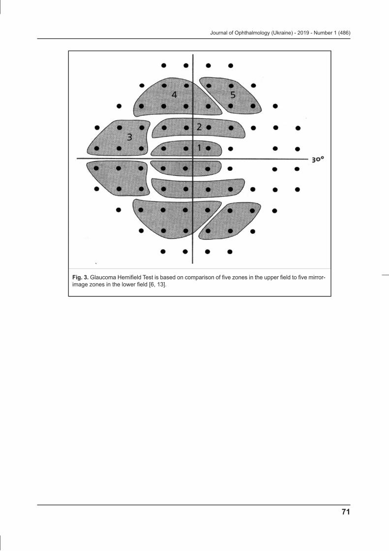
One of the major parameters which can signify a glaucomatous character of the revealed visual field defects is the Glaucoma Hemifield Test (GHT). The test is based on the fact that visual field defects are asymmetrical in glaucoma. GHT compares light sensitivity in five zones in the upper hemifield to findings in mirror-image zones in the inferior visual field (Fig.3). In norm, light sensitivity is almost the same in two hemifields while it is decreased locally in one of the hemifields in glaucoma [6, 13, 14].
The findings on light sensitivity in the paired zones are compared and the results are interpreted as Within Normal Limits, Outside Normal Limits, and Borderline (Fig. 2F). Sometimes, in the presence of optic medium transparency disorders, uncorrected refraction errors, or diffuse damage to the retina and optic nerve, visual fields are described to have General Reduction of Sensitivity. In rare cases, the GHT describes visual fields as having Abnormal High Sensitivity when the test has been performed incorrectly by a patient (in the presence of a great number of false-positive errors).
Journal of Ophthalmology (Ukraine) - 2019 - Number 1 (486)
67
Quantitative indices of visual field defect assessment are global indices including MD (Mean Deviation), PSD (Pattern Standart Deviation), and VFI (Visual Field Index) (Fig. 2 G).
Mean Deviation is a total quantitative index of the Total Deviation Plot which shows the average difference from the normal value in the patients’ particular age group. A negative MD value indicates that total light sensitivity is less than normal.
Pattern Standard Deviation is based on the findings of the Pattern Deviation Plot and provides information about localized field defects. A PSD value is always positive; its significant value is given similar to that of the MD values.
Visual Field Index was included in the Humphrey perimeter STATPAC by Bengtsson B. and Heijl A. in 2008 and its purpose is to assess glaucoma progression rates [7, 9, 14]. To calculate VFI, the light sensitivity values in each test point are expressed as a percentage of age-normal and all test point values are averaged with a probability of deviation from the norm <5%. VFI=100% indicates that light sensitivity is normal. In the presence of test points with decreased light sensitivity, the VFI value is lower.
Some words should be said about the reliability and accuracy of the test results, ignoring which can lead to incorrect interpretation of the findings and, as a consequence, to diagnostic errors.
First of all, it should be noted that the central visual field within 30° must always be tested with appropriate near-distance correction of refractive error. If this requirement is ignored, there can be false visual field defects and, consequently, overdiagnosis. The power of a trial lens is calculated automatically by the perimeter according to the patient’s refraction. The power of a trial lens is noted in the printout heading (Fig. 2).
Other indices to see if the test results are reliable are false positive (False-POS) and false-negative (False-NEG) errors (Fig. 2A). False positive errors occur when patients' responses are recorded in the absence of a presented stimulus; false negative errors occur when no response is recorded to a brighter stimulus at a test point location where a response to a less bright stimulus has already been recorded. A rate of false positive and false negative errors must not exceed 15% and 20%, respectively; otherwise, it is considered that test results are compromised [14, 18, 22].
It is known that glaucomatous visual field defects correspond topographically to the path of retinal nerve fibres. Fibres from the temporal and most nasal retina follow toward the optic disc and arc around the macula while only a small number of axons of nasal macular ganglion cells have a radial path. Superior and inferior neurons are separated by a horizontal raphe which runs from the yellow spot to the retinal periphery. Damage to nerve fibre bundles in, as a rule, superior and inferior poles of the disc lead to common glaucomatous visual field defects including paracentral scotomas, nasal steps, arcuate scotomas, and temporal sectoral defects. Diffuse
damage to neurons causes a diffuse decrease in visual field light sensitivity [8, 13, 21].
Early changes of glaucomatous visual field defects can be manifested as asymmetry in light sensitivity between two eyes with absolutely normal values of GHT, MD, PSD, and VFI in both eyes. In such cases, in data interpretation, not only asymmetry in the MD and PSD values must be considered but also the entirety of clinical data including intraocular pressure rates, optic disc ophthalmoscopy, and data of optical coherence tomography (OCT) [8].Generalized diffuse depression is a common visual field defect in glaucoma. However, the detected visual field loss can be considered as a result of diffuse glaucomatous damage to the optic nerve only after excluding such factors as optical media opacity, high refractive errors, and a constricted or dilated pupil since they also can cause diffuse loss of sensitivity [8, 13].
Glaucomatous visual field loss is characterized by asymmetrical light sensitivity in superior and inferior hemifields. In this case, a Single Field Analysis printout gives such GHT messages as Borderline and Outside Normal Limits. As an example, Figure 2 demonstrates visual fields of a 71-year-old patient with stabilized primary open-angle glaucoma and shows local sensitivity loss in the inferior nasal quadrant with an arcuate scotoma; GHT is Outside Normal Limits.
Damage to nerve fibres is local in the presence of cupping of the optic disc that leads to a paracentral scotoma in the visual fields which is more often located in the nasal hemifield [8, 13].
Nasal steps are defects when the difference in light sensitivity between superior and inferior hemifields of the nasal visual field is strongly-pronounced across the horizontal meridian (Fig. 4)
Extension of the optic cup to the rim of the disc will result in loss of nerve fibres and, consequently, in cupping. Thus, a deep arcuate defect, which is connected to the blind spot and known as the Bjerrum scotoma, is detected in the visual field. The arcuate scotoma usually courses around the point of fixation and ends abruptly at the horizontal meridian corresponding to the temporal raphe of the retina. Extension of the cup to both poles of the disc leads to a ‘double arcuate’ scotoma (superior and inferior).
Glaucomatous optic neuropathy progression results in increased death of nerve fibres and, therefore, the area and depth of visual field loss are enlarged. So, there occurs a complete defect of the nerve-fibre bundles which develops into an altitudinal defect and deep depression of the entire visual field. A wedge-shaped defect should be noted as a rare visual field defect in glaucoma since it is recorded only in 3 % of cases [8, 13].
None of the visual field defects which can occur in glaucoma is 100% specific to this disease. Visual field loss can be associated with any damage to the optic nerve. That is why, only a comprehensive examination, including intraocular pressure measurements, optic disc ophthalmoscopy, OCT, family history, and other risk
Journal of Ophthalmology (Ukraine) - 2019 - Number 1 (486)
68
factors, can confirm a glaucomatous nature of visual field loss. Choplin N.T. et al. have reported that visual field defects, which are most common for glaucoma, are arcuate scotomas (90%), nasal steps (54%), paracentral defects (41%), and arcuate enlargement of the blind spot (30%) [8]. Guided Progression Analysis (GPA) (Fig. 4).
Humphrey Guided Progression Analysis is advanced software designed to highlight any changes in the visual field loss in glaucoma patients, to detect and to assess the statistically significant progression of visual field loss in optic neuropathy progression. GPA is based on the comparative analysis of at least three visual field tests (Central-24/Central-30 SITA Standard). The software is based on a knowledge that was gained through extensive multi-centre clinical trials performed in medical centres of North America, Europe, and Asia [4].
GPA consists of two parts: Event Analysis and Trend Analysis.
Event Analysis is designed to filter out the changes in the visual field retests and based on detecting statistically significant differences in light sensitivity at each point of the Pattern Deviation Plot between consequent tests through the Progression Analysis Probability Plot (Fig. 4A).
Significant changes in a test point are indicated using a set of triangle symbols; half-filled and filled triangles, repeated in, respectively, two or three consecutive Follow-up exams, identify statistically significant deterioration in the test point (Fig. 4). A GPA alert, “No Progression Detected”, “Possible Progression” or “Likely Progression,” appears below each exam analysis.
Trend Analysis determines the current trends in visual field changes for the next 3-5 years, based on the VFI regression analysis. The VFI values are plotted to quantify the Rate of Progression and provide a visual trend of the progression pattern (Fig. 4B).
Figure 4 demonstrates, as an example, a GPA Summary Report of a 56-year-old patient with primary open-angle glaucoma for the period from 2014 to 2018. The first visual field test, dated August 19, 2014, revealed no significant defects but mild depression in the nasal hemifield; GHT reported Within Normal Limits with MD = -1.59 dB, PSD = 2.21 dB, VFI = 98%. A retest in a year's time, on May 07, 2015, showed a stable visual field with MD = -0.68 dB, PSD = 2.16 dB, VFI = 98%; however, the GHT alert message was Borderline. For the following two years, no changes were recorded as well; the patient’s intraocular pressure was drug-corrected. The last follow-up test, on June 07, 2018, revealed a sharp local deterioration of sensitivity in the superior nasal field with a deep nasal step and an arcuate scotoma; the global indices were also worsened significantly and equalled: MD = -4.15 dB, PSD = 9.31 dB, and VFI = 87%. Visual field loss was confirmed by the Progression Analysis Probability Plot and a regression line of the VFI. The GPA analysis reported Possible Progression.
Conclusion
Modern automated computerized static perimetry using Humphrey Visual Field Analyzer II, which has been recognized as a gold standard of perimetry for visual field testing in glaucoma, makes it possible to highlight and to quantify visual field loss, including any changes at early stages of glaucoma. Guided Progression Analysis, a software package for the Humphrey Field Analyzer, provides the possibility to identify and to quantify statistically significant progressive visual field loss in glaucoma patients.
Agayeva F.A. [Advantages of humphrey perimeter in the diagnosis and monitoring of glaucoma (literature review)] // Oftalmologiya. Elmi-praktik jurnal. 2015;3:130–6. Russian.
2. Kurysheva NI. [Perimetry in diagnostics of glaucomatous optic neuropathy]. M.; 2015. Russian.
4. Serdyukova SA, Simakova SA. [Computer Perimetry in the diagnosis of primary open-angle glaucoma]. A Serdyukova, Svetlana & L Simakova, Irina. (2018). Computer perimetry in the diagnosis of primary open-angle glaucoma. Ophthalmology journal. 11. 54-65. 10.17816/OV11154-65.
5. Alencar LM, Medeiros FA. The role of standard automated perimetry and newer functional methods for glaucoma diagnosis and follow-up. Indian J Ophthalmol. 2011;59: S53-58.
6. Asman P, Heijl A. Glaucoma Hemifield Test. Automated visual field evaluation. Arch Ophthalmol. 1992;110:812-9.
7. Bengtsson B, Heijl A. A visual field index for calculation of glaucoma rate of progression. Am J Ophthalmol. 2008;145:343–53.
8. Choplin NT, Lundy DC. Atlas of glaucoma. Second Edition. - Informa UK Ltd, 2007. 343 р.
9. Flammer J. The concept of visual field indices./ Graefes Arch Clin Exp Ophthalmol. 1986;224:389–92.
10. Flammer J, Drance SM, Augustiny L, Funkhouser A. Quantification of glaucomatous visual field defects with automated perimetry. Invest Ophthalmol Vis Sci. 1985;26:176–81.
11. Gloor BP. Franz Fankhauser: the father of the automated perimeter. Surv Ophthalmol. 2009;54 (3):417-25.
12. Heijl А, Patella VM, Bengtsson B. The Field Analyzer Primer: Effective Perimetry. Dublin: Carl Zeiss Meditec Inc; 2012.
13. Hejl A, Patella VM. Essential Perimetry. The Field Analyzer Primer. Third edition. Carl Zeiss Meditec Inc., 2002. 164 p.
14. Humphrey Field Analyzer. II-i series System Software Version 5.1. User Manual. Carl Zeiss Meditec, Inc., 2012.
15. Imaging and Perimetric Society Standarts and Guidelines 2010. Available at: http://www.perimetry.org/GEN-INFO/standards/IPS-Standards-2010.HTM
16. Johnson CA, Adams AJ, Casson EJ, et al. Progression of early glaucomatous visual field loss as detected by blue-on-yellow and standard white-on-white automated perimetry. Arch Ophthalmol. 1993;111:651–656.
17. Johnson ChA, Wall M, Thompson HS. A History of Perimetry and Visual Field Testing. Optometry and Vision Science. 2011;88(1):Е8-Е15.
Journal of Ophthalmology (Ukraine) - 2019 - Number 1 (486)
69
18. Kahook MY, Noecker RJ. How Do You Interpret a 24-2 Humphrey Visual Field Printout? Glaucoma Today. 2007; November/December: 57-62.
19. Nathan J. Hippocrates of the to Duke-Elder: an overview history of glaucoma. Clin Exp Optom. 2000;83(3):116-8.
20. Schiefer U, Patzold J, Dannheim F, Artes P, Hart W. Conventional Perimetry. Part I: Introduction – Basic Terms. Der Ophthalmologe. 2005;102(6):627-46.
21. Visual fields: examination and interpretation / edited by Thomas J. Walsh. 3rd ed. Oxford University Press, 2011. 312 p.
23. Weijland A, Fankhauser F, Bebie H, Flammer J. Automated Perimetry. Visual Field Digest. - Fifth Edition. 2004. 198 р.
24. Weinreb R, Greve E, editors. Progression 8th consensus report of the world glaucoma Amsterdam: Kugler Publications; 2011.
Fig. 1. Relationship between stimulus luminance (asb) and differential light sensitivity (db) in the Humphrey Visual Field Analyzer II [13].
Limit of foveal vision
Normal range of threshold sensitivity in the central visual field
Typical range of threshold sensitivity in visual defects
Maximum stimulus brightness provided by the perimeter
Absolute blindness
5 log. unit
4 log. unit
3 log. unit
2 og. unit
1 log. unit
0
Apostilb (asb) Decibel (dB)
Journal of Ophthalmology (Ukraine) - 2019 - Number 1 (486)
70
Fig. 2. Visual field of a 71-year-old female patient with primary open-angle glaucoma, showing a local decrease in light sensitivity in inferior nasal quadrant and indications of an arcuate scotoma
Journal of Ophthalmology (Ukraine) - 2019 - Number 1 (486)
71
Fig. 3. Glaucoma Hemifield Test is based on comparison of five zones in the upper field to five mirror-image zones in the lower field [6, 13].
Journal of Ophthalmology (Ukraine) - 2019 - Number 1 (486)
72
Fig. 4. GPA Summary Report for a 56-year-old patient with primary open-angle glaucoma for the period from 2014 to 2018