Practical approaches to varying network size incombinatorial key predistribution schemes

Kevin Henry1, Maura B. Paterson2, and Douglas R. Stinson?3

1 David R. Cheriton School of Computer ScienceUniversity of Waterloo, Waterloo, Ontario, N2L 3G1, Canada

k2henry@cs.uwaterloo.ca2 Department of Economics, Mathematics and Statistics

Birkbeck, University of London, Malet Street, London WC1E 7HX, UKm.paterson@bbk.ac.uk

3 David R. Cheriton School of Computer ScienceUniversity of Waterloo, Waterloo, Ontario, N2L 3G1, Canada

dstinson@math.uwaterloo.ca

Abstract. Combinatorial key predistribution schemes can provide apractical solution to the problem of distributing symmetric keys to thenodes of a wireless sensor network. Such schemes often inherently suitnetworks in which the number of nodes belongs to some restricted setof values (such as powers of primes). In a recent paper, Bose, Dey andMukerjee have suggested that this might pose a problem, since discardingkeyrings to suit a smaller network might adversely affect the propertiesof the scheme.In this paper we explore this issue, with specific reference to classes of keypredistribution schemes based on transversal designs. We demonstratethrough experiments that, for a wide range of parameters, randomlyremoving keyrings in fact has a negligible and largely predictable effect onthe parameters of the scheme. In order to facilitate these computations,we provide a new, efficient, generally applicable approach to computingimportant properties of combinatorial key predistribution schemes.We also show that the structure of a resolvable transversal design canbe exploited to give a deterministic method of removing keyrings toadjust the network size, in such a way that the properties of the resultingscheme are easy to analyse. We show that these schemes have the sameasymptotic properties as the transversal design schemes on which theyare based, and that for most parameter choices their behaviour is verysimilar.

Keywords: wireless sensor network, key predistribution scheme, com-binatorial design

1 Introduction

In this paper, we consider wireless sensor networks (WSNs) consisting of a largenumber m of identical sensor nodes that are randomly deployed over a target

? D. Stinson’s research is supported by NSERC discovery grant 203114-11

area. After deployment, each node communicates in a wireless manner with othernodes that are within communication range, thus forming an ad hoc network.Due to the wireless nature of the communication, it is desirable for cryptographictools to be used for provision of secrecy, data integrity, and/or authentication.The nodes’ restricted computational ability and battery power mean that, inmany situations, it is preferable to use symmetric algorithms rather than relyingon more computationally-intensive public key techniques. This requires nodesto share keys; one standard approach to providing such keys is the use of a keypredistribution scheme (KPS), in which keys are stored in the nodes’ keyringsprior to deployment. For example, in the seminal scheme of Eschenauer andGligor [4], the keys are randomly drawn from a common keypool.

After the nodes have been deployed, nodes that are within communicationrange execute a shared key discovery protocol to determine which keys theyhave in common. Two nodes that share at least η keys (for some predeterminedintersection threshold η ≥ 1) use all their common keys to derive a new key thatis used to secure communication between them. This is referred to as a securelink between these nodes. There exists a large quantity of literature relating tothe construction of KPSs for WSNs; surveys include [2, 7, 10].

KPSs based on combinatorial structures such as designs or codes have beenstudied as an alternative to random schemes (see [6, 9] for surveys of combinato-rial schemes). Such schemes have several advantages over the random schemes:for instance, they make it possible to prove the scheme has desirable propertiesrelating to connectivity and resilience, they enable more efficient discovery ofshared keys, and they reduce the amount of randomness required when instan-tiating the schemes [5].

Key predistribution schemes for WSNs are typically evaluated using certainmetrics that relate to the performance of the resulting networks. Firstly, it isdesirable to restrict the total amount of memory each node must use for stor-ing keys/keying material. Secondly, after the nodes have been deployed, it isdesirable for there to be as many secure links as possible between neighbouringnodes, so as to increase the (secure) connectivity of the resulting network. Theextent to which a KPS facilitates achieving this objective is frequently measuredin terms of the quantity Pr1, which denotes the probability that any two givennodes share at least η common keys.

Finally, we wish to measure the scheme’s ability to withstand adversarialattack. A widely studied attack model, which we follow in this paper, is thatof random node capture [4], where the adversary can eavesdrop on all communi-cation in the network, and can also comprise random nodes in order to extractany keys/keying material they contain. The resilience of a KPS in the face of anattacker is expressed in terms of the quantity fail(s), which is defined to be theprobability that a randomly chosen link is broken when an attacker compromisess nodes uniformly at random, and then extracts their keys.

For simplicity, we focus particularly on fail(1) in this work. In this case, alink {A,B} is broken by another node C when A ∩ B ⊆ C, where A,B and Cdenote the sets of keys held by the three corresponding nodes.

There is an inherent tension between the need to provide good connectivityand the need to maintain a high level of resilience without requiring an excessivenumber of keys to be stored. Designing a KPS involves finding a scheme thatdelivers a good tradeoff between these properties, and which is sufficiently flexibleto be useful for a range of practical choices of parameters such as network size,available storage and desired level of security.

One feature of combinatorial schemes that could be viewed as a drawback isthe fact that, due to the structure of the combinatorial object used, the numberof nodes in the scheme may be required to be of a particular form, such as apower of a prime, for example. If the number n of nodes in the network in whichwe wish to employ such a scheme is not of this form, then the most commonlysuggested remedy is to take the smallest number of that form that is largerthan n, and simply select some (randomly chosen) subset of n keyrings from theresulting scheme (e.g., see [5]). In a recent paper [1], Bose, Dey and Mukerjee havesuggested that removing keyrings in this manner from a combinatorial schememay adversely affect its properties, thus negating some of the main benefits ofsuch schemes. Instead, they propose a deterministic KPS in which various blockdesigns are combined to give a scheme in which the number of keyrings can bevaried directly in a more flexible manner.

In this paper, we examine more closely the actual effects of removing keyringsfrom a combinatorial KPS. We focus specifically on the family of schemes pro-posed by Lee and Stinson based on transversal designs [5], since they have beenshown to behave well for a wide range of parameters [9]. In Section 2, we exploitthe structure of resolvable transversal designs to propose a deterministic methodfor selecting keyrings to remove from the schemes of Lee and Stinson withoutunduly affecting their performance. The properties of these modified schemes areeasy to analyse using the framework established in [9], and we exploit this fea-ture to compare their performance directly with the the combinatorial schemesfrom which they were derived, demonstrating that they yield a family of schemeswith a flexible choice of parameters whose properties compare favourably withthose of existing schemes.

In addition, for a broad range of parameter choices, we consider networksconsisting of various numbers of nodes with keyrings chosen uniformly at randomfrom transversal design KPSs, and we compute the mean and standard deviationof the resulting values of the security and performance metrics for these schemes.The results, given in Section 3.2, demonstrate that the change in these metricsas keyrings are removed is in fact very limited, and largely predictable.

Computing properties of schemes obtained by randomly deleting some num-ber of keyrings from a combinatorial scheme can be time-consuming. Therefore,in Section 4 we describe a new approach to facilitate the efficient evaluation ofmetrics for connectivity and resilience in general KPSs. This approach is basedon some new formulas for these metrics that are of independent interest.

1.1 Overview of the Construction and Analysis of CombinatorialKey Predistribution Schemes

A set system (X,A) consists of a finite set X of points, together with a finiteset A of subsets of X, which are known as blocks. A set system can be used toconstruct a KPS by associating each key in a certain keyspace with an elementof X and each node with an element of A, so that a node is preloaded with thekeys that correspond to points lying in its corresponding block. The point x actsas a key identifier for the corresponding secret key. Key identifiers (and whichnodes hold which key identifiers) are public information, whereas the values ofthe keys are secret (known only to the nodes that hold them).

Example 1. Let

X = {1, 2, 3, 4, 5, 6, 7, 8, 9}, and

A = {123, 456, 789, 147, 258, 369,

159, 267, 348, 168, 249, 357}.

Then (X,A) is a set system in which there are nine points and twelve blocks.Each block contains three points. The associated KPS will have 12 nodes, eachof which possesses three of the nine secret keys.

It is easy to see that, in this model, the Eschenauer-Gligor scheme [4] is ob-tained when the underlying set system consists of n random k-subsets of the v-setX. On the other hand, combinatorial key predistribution schemes are typicallybased on set systems arising from combinatorial objects with nice properties thatensure the resulting schemes perform well and are amenable to analysis. Partic-ular examples of combinatorial objects that have been proposed for use in keydistribution in this way include projective planes, generalised quadrangles, con-figurations, common intersection designs, transversal designs of strength 2 or 3,partially balanced incomplete block designs, inversive planes, orthogonal arrays,Reed-Solomon codes, mutually-orthogonal Latin squares, and rational normalcurves in projective spaces (see [9] for a survey and analysis of such schemes).

In this paper, we focus mainly on transversal designs, which we define now.

Definition 1. Let t, n and k be positive integers such that t ≤ k ≤ n. A transver-sal design TD(t, k, n) is a triple (X,H,A), where X is a finite set of cardinalitykn, H is a partition of X into k parts (called groups) of size n and A is a setof k-subsets of X (called blocks), which satisfy the following properties:

1. |H ∩A| = 1 for every H ∈ H and every A ∈ A, and2. every subset of t elements of X from t different groups occurs in exactly one

block in A.

The parameter t is called the strength of the transversal design.

We note that transversal designs are equivalent to other familiar combinato-rial objects such as orthogonal arrays and maximum distance separable (MDS)codes; see [9, §2.7] for further discussion on these equivalences.

Example 2. Lee and Stinson [5] proposed a family of combinatorial KPSs basedon transversal designs TD(2, k, p). The set systems they use can be constructedexplicitly as follows:

For p a prime and k an integer with 2 ≤ k ≤ p we construct a TD(2, k, p) byletting the points be all elements of the form (a, b) where a ∈ {0, 1, . . . , k − 1}and b ∈ Zp. The transversal design has p2 blocks, which are given by the sets ofthe form

Ai,j = {(x, ix+ j (mod p))|0 ≤ x ≤ k − 1}.

This construction can be generalised in an obvious way by replacing Zp by thefinite field GF(n). Hence, we can obtain a transversal design TD(2, k, n) with n2

blocks for any prime power n. It is straightforward to show that in this schemeany two nodes share either 1 key or 0 keys; as such we specify that η = 1 andhence two neighbouring nodes form a secure link if they share one common key.

To construct a transversal design of strength 3 (a TD(3, k, p)) the points aretaken to be all elements of the form (a, b) where a ∈ {0, 1, . . . , k−1} and b ∈ Zp,as before. For each of the p3 polynomials f in Zp[x] of degree at most 2 we obtaina block by taking the set of points of the form

Af = {(x, f(x) (mod p))|0 ≤ x ≤ k − 1}.

Once again, we can replace Zp by the finite field GF(n) in this construction andobtain a TD(3, k, n) for any prime power n. Two nodes in this scheme shareeither 0, 1 or 2 keys. Hence we can choose to use an intersection threshold ofeither η = 1 or η = 2 for specifying the minimum number of keys that must beshared by two nodes before they can form a secure link.

The values of fail(1) and Pr1 for these schemes, in the case of strength 2 withη = 1 and strength 3 with η = 1 or η = 2, are given in Table 1.

For the transversal designs TD(t, k, n) for both t = 2 and t = 3 describedabove, the points of the design can be partitioned into k subsets Hi, for 0 ≤ i ≤k − 1, by setting

Hi = {(i, b)|b ∈ GF(n)}.

These sets Hi are known as the groups of the transversal design. It is straight-forward to show that each subset of t points of the transversal design from tdifferent groups occur together in exactly one block of the transversal design.

Example 3. Bose et al. [1] proposed a family of KPSs obtained by combining ηdesigns that are the duals of designs derived from association schemes. For thesake of clarity, we will restrict ourselves to the specific instantiation in which thedesigns are all copies of a TD(2, k, n).

In the case of η = 1, the Bose et al. scheme instantiated with a TD(2, k, n)coincides exactly with Lee and Stinson’s transversal design scheme.

For η = 2, they take two copies of a TD(2, k, n) and construct a new setsystem by letting the set of points be the union of the sets of points of each

of the designs, and by letting the blocks be given by all possible unions of theform B1 ∪ B2 where B1 is a block of the first TD(2, k, n) and B2 is a block ofthe second TD(2, k, n). This scheme has 2kn points, and n4 blocks. Each blockcontains 2k points, and two blocks intersect in either 0, 1, 2, k, or k + 1 points.

As observed in [5], combinatorial schemes possess several distinct advantagesas compared to random schemes such as Eschenauer-Gligor:

– the deterministic nature and regular structure of combinatorial schemes en-sure that the precise values of metrics of the scheme such as fail(1) and Pr1can be computed exactly, rather than simply the expected value of thesequantities;

– combinatorial schemes reduce the quantity of random numbers that must begenerated in setting up the scheme;

– most importantly, for many combinatorial schemes, their regular structureleads to very efficient algorithms for performing tasks such as shared keydiscovery once the nodes are deployed.

As such, combinatorial schemes can represent an efficient and effective way ofestablishing keys in many WSN scenarios.

A survey and analysis of many existing combinatorial schemes was carried outin [9]. The concept of a partially balanced t-design (PBtD) was introduced, andexplicit formulas for evaluating fail(1) and Pr1 were given for any combinatorialscheme that can be constructed from a PBtD.

Definition 2. For positive integers v, k, t and λi with 0 ≤ i ≤ t − 1, a t −(v, k, λ0, λ1, . . . , λt−i)-partially balanced t-design is a pair (X,A) with the fol-lowing properties:

1. X is a finite set whose elements are referred to as points, and A is a finiteset of k-subsets of X; its elements are referred to as blocks.

2. There are λ0 blocks in A.3. For 1 ≤ i ≤ t− 1, each subset of i points of X occurs in either no blocks, or

in exactly λi blocks.4. For t ≤ i ≤ k, each subset of i points occurs in either 0 or 1 blocks.

Paterson and Stinson [9] showed that a wide range of existing combinatorialKPSs (including KPSs constructed from transversal designs) could be modelledas PBtDs. The advantage of doing so is that the properties of these schemes caneasily be evaluated and compared with the aid of the formulas given in [9]. Theresulting values for a range of schemes are given in Table 1. The transversal-design based schemes described in Example 2 were shown to provide a gooddegree of flexibility for the construction of KPSs relative to other PBtDs, sincethey are easily constructed for a wide range of useful parameters, the block sizecan be chosen independently of the network size, and the values of t and η canalso be varied independently.

The KPSs of Bose et al. [1] are not PBtDs, and hence they cannot be analyseddirectly using the approach of [9]. One of the motivations behind their schemes is

to provide constructions that can yield KPSs for a flexible choice of network size;in [1], they note that “the number of nodes need not be of the particular formsp2 or p3, with p prime or prime power”. The traditional view of combinatorialconstruction of KPSs is that, provided a range of parameters is available, thenif a specific network size n is desired it suffices to choose parameters to givea scheme that suits a network of size greater than n and simply discard theunneeded keyrings. Bose et al. [1] object (with particular reference to [5]) that“if we then discard the unnecessary node allocations to get the final scheme foruse, this final scheme will not preserve the Pr1 and fail(s) values of the originalscheme and hence the properties of the final scheme in this regard can becomequite erratic” [1]. One main goal of our paper is to refute this statement.

1.2 Outline of the Paper

In Section 2, we present two approaches to increasing the flexibility of combi-natorial predistribution schemes based on transversal designs. One approach israndomized and the other is deterministic. In Section 3, we perform extensivecomparisons of our generalized constructions to the original transversal designschemes. In Section 4, we derive new formulas that facilitate the computation ofmetrics for connectivity and resilience for arbitrary key predistribution schemesbased on set systems. Finally, Section 5 is a short conclusion.

2 Two Approaches to Varying the Network Size in KPSsbased on Transversal Designs

In this section we consider two distinct approaches to varying the network sizein the transversal design-based KPSs of Lee and Stinson. One option is to usethe standard approach of randomly removing blocks from the design.

Scheme 1 (Random scheme). Suppose a KPS is desired for a network con-taining m nodes. Let n be the smallest prime power satisfying n2 ≥ m. Then byconstructing a TD(2, k, n) and selecting a subset of m blocks uniformly at randomwe obtain a set system that can be used to provide a KPS for the network.

Similarly, we can construct a KPS for this network based on a transversaldesign of strength 2 by taking n to be the smallest prime power with n3 ≥ m,and then selecting m blocks uniformly at random from the set of blocks of aTD(3, k, n).

The benefits of such an approach include its simplicity and the fact that itcan be applied for any value of m. It is a very natural approach, given that itmirrors precisely the commonly anticipated situation in which a small number ofnodes may fail or run out of power after deployment. We will see that this schemeperforms well in practice: in Section 3.2 we demonstrate that for a wide rangeof parameter choices, restricting to a random subset of blocks of a TD(2, k, n)does not adversely affect the expected performance of schemes based on these

designs. Furthermore, we still retain some desirable properties of combinatorialschemes such as efficient shared key discovery.

One of the other underlying motivations of using combinatorial designs toconstruct KPSs is the fact that their deterministic and highly structured natureallows us to guarantee the values they attain for metrics such as fail(1) and Pr1. Ifblocks are deleted at random, we lose these guarantees, even though diminishedperformance is very unlikely. In this section we propose a second technique, toovercome this possible drawback. We demonstrate how to exploit the structureof transversal designs in order to select subsets of the blocks deterministically insuch a way that the precise performance of the resulting structure is straightfor-ward to evaluate. Specifically, we will make use of resolvable transversal designsto accomplish this objective.

2.1 Resolvable Transversal Designs of Strength 2

Definition 3. A transversal design TD(2, k, n) is said to be resolvable if it ispossible to partition the blocks of the design into sets B1,B2, . . . ,Bn, such thateach point of the design belongs to precisely one block in each set. The sets Biare known as parallel classes of the design.

Resolvable transversal designs have previously been exploited for construct-ing KPSs suited for networks where there is group deployment of nodes; see [8].The transversal design KPSs proposed by Lee and Stinson do not require theresolvability property; however, the transversal designs TD(2, k, n) used in [5]are in fact resolvable.

Example 4. For the TD(2, k, n) described in Example 2, the parallel classes ofblocks are given by

Bi = {Ai,j |j ∈ GF(n)}, i ∈ GF(n).

It is straightforward to see that no point lies in two distinct blocks of a givenparallel class, since if a point (x, y) were in blocks Ai,j and Ai,h, this wouldimply that y = ix+ j and also y = ix+ h, whence j = h.

A resolvable transversal design TD(2, k, n) has n parallel classes with n blocksin each class. We propose using such designs for key predistribution as follows:

Scheme 2 (Linear scheme). We construct a set system for use in a KPS bystarting with a resolvable TD(2, k, n), where n is a prime power. Let ` be aninteger between 1 and n. Select ` parallel classes of blocks of the design, and letthe blocks in these parallel classes be the blocks of the set system. We refer tothe resulting set system as a TD(2, k, n, `).

As each parallel class contains n blocks, this means that Scheme 2 yieldsa KPS with `n keyrings. This number can be varied as required by choosingan appropriate value of `: roughly speaking, we require that n ≥

√m and ` ≈

m/n. One nice feature of this method of choosing blocks is that the resulting

incidence structure is in fact a PBtD, and hence its properties can be determinedin a straightforward manner simply by using the formulas given in [9]. We nowperform this analysis to show that Scheme 2 performs well even for comparativelysmall values of `.

Theorem 1. A TD(2, k, n, `) is a 2-(kn, k, `n, `)-PBtD

Proof. Take ` parallel classes of blocks from a resolvable TD(2, k, n), and let Abe the set of blocks in these parallel classes. Let X be the set of points in theTD(2, k, n); we note that X contains kn points. Now, A contains λ0 = `n blocks,each containing k points. Every point of X is contained in precisely one blockin each parallel class, and hence is contained in precisely λ1 = ` blocks of A.Furthermore, since each pair of points in X is contained in either 0 or 1 blocksof the TD(2, k, n), it follows that any pair of points is contained in either 0 or 1blocks of A. Thus (X,A) satisfies all the properties of a 2-(kn, k, `n, `)-PBtD.

The values of fail(1) and Pr1 for a PBtD are easy to compute systematicallyusing the explicit formulas given in [9]. For a given block B of a PBtD and apoint C on that block, denote by µ′(1) the number of blocks A of the PBtDsuch that A∩B = {C} (it was shown in [9] that this value is independent of thechoice of point and block.) Define a link to be a pair of blocks with nonemptyintersection. We let L denote the total number of links in a PBtD, we let αdenote the number of links in which a given block B is contained, and we letβ denote the number of links {A,C} with B 6= A,C such that A ∩ C ⊂ B(again, these values do not depend on the specific choice of B). Then, applyingthe formulas of [9] to a 2-(kn, k, `n, `)-PBtD, we have:

µ′(1) = λ1 − 1 = `− 1,

α = kµ′(1) = k(`− 1),

β = µ′(1)

(λ12− 1

)k = (`− 1)

(`

2− 1

)k,

L =bα

2=`nk(`− 1)

2,

fail(1) =β

L− α=

`− 2

`n− 2,

Pr1 =α

b− 1=k(`− 1)

`n− 1.

In the case where ` = n, a TD(2, k, n, `) is simply a TD(2, k, n), and henceScheme 2 is a generalisation of the corresponding scheme of Lee and Stinson.The formulas computed above for fail(1) and Pr1 can be seen to agree with thecorresponding formulas for Lee and Stinson’s scheme in the case where ` = n.

2.2 Transversal Designs of Higher Strength

Just as in the case of transversal designs of strength 2, it is possible to determin-istically select subsets of blocks from transversal designs of higher strength, such

as the TD(3, k, n) suggested for use in key predistribution by Lee and Stinson,in a way that allows flexibility in the number of keyrings of the resulting scheme,while still maintaining good performance. We begin by illustrating a useful ap-proach to partitioning the blocks of the TD(3, k, n) described in Example 2.

Example 5. Let n be a prime power and let X be the set of points of one of theTD(3, k, n) whose construction is described in Example 2. We can partition theblocks of this design into sets B1,B2, . . . ,Bn by defining

Bi = {Af |f(x) = ix2 + ax+ b for some a, b ∈ GF(n)}, i ∈ GF(n).

We show, for each i, that the incidence structure (X,Bi) is a TD(2, k, n), withthe same groups as the original TD(3, k, n). Suppose this is not the case. Thenthere is a pair {(x,A), (y,B)} (where x 6= y) that appears in two blocks of thesame Bi. So we have

ix2 + ax+ b = A = ix2 + cx+ d and iy2 + ay + b = B = iy2 + cy + d.

From this, we get

ax+ b = cx+ d and ay + b = cy + d.

Since x 6= y, we have a = c, which implies b = d. Therefore the two blockscoincide and we have a contradiction.

Scheme 3 (Quadratic scheme). Let n be a prime power. Starting with aTD(3, k, n), we define a set system by letting ` be an integer between 1 and n,selecting ` of the sets Bi, and letting A be the set of blocks in these ` sets. Werefer to the incidence structure (X,A) as a TD(3, k, n, `). Using a TD(3, k, n, `)for constructing a KPS in the standard way yields a scheme with `n2 keyrings,for which we can choose an intersection threshold of either η = 1 or η = 2.

As before, this method of selecting blocks yields a structure that is easy toanalyse:

Theorem 2. A TD(3, k, n, `) is a 3-(kn, k, `n2, `n, `)-PBtD.

Proof. A TD(3, k, n, `) consists of a set of kn points, together with ` disjoint setsof n2 blocks of k points, and thus has `n2 blocks in total. Every point of theTD(3, k, n, `) is contained in n blocks in each of these sets, and therefore is con-tained in `n blocks in total. If a pair of points belong to a group of the underlyingTD(3, k, n) then they do not occur together in any block of the TD(3, k, n, `). Iftwo points lie in different groups, then in each of the ` sets Bi there is preciselyone block that contains them. Thus any pair of points occurs together in either0 or ` blocks of the TD(3, k, n, `). Finally, any set of three points occur togetherin either 0 or 1 blocks of the TD(3, k, n) and thus also occur together in 0 or 1blocks of the TD(3, k, n, `).

This allows us to use the formulas of [9] to compute fail(1) and Pr1. Definingµ′(2) to be the number of blocks C whose intersection with a given block B is agiven set S ⊂ B of two points, we have

µ′(2) = λ2 − 1 = `− 1,

µ′(1) = λ1 − 1− (k − 1)µ′(2) = `n− 1− (k − 1)(`− 1).

For a KPS with intersection threshold η = 2 we have

α =

(k

2

)µ′(2) =

(k

2

)(`− 1),

β = µ′(2)

(λ22− 1

)(k

2

)= (`− 1)

(`

2− 1

)(k

2

),

L =bα

2=`n2(`− 1)

2

(k

2

),

fail(1) =β

L− α=

`− 2

`n2 − 2,

Pr1 =α

b− 1=k(k − 1)(`− 1)

2(`n2 − 1).

Using intersection threshold η = 1 gives

α = kµ′(1) +

(k

2

)µ′(2) = k(`n− 1)−

(k

2

)(`− 1),

β = µ′(1)

(λ12− 1

)k + µ′(2)

(λ22− 1

)(k

2

),

= (`n− 1− (k − 1)(`− 1)) k

(`n

2− 1

)+ (`− 1)

(`

2− 1

)(k

2

),

L =bα

2=`n2

(k(`n− 1)−

(k2

)(`− 1)

)2

,

fail(1) =β

L− α=

2(`n− 1)(`n− 2)− (k − 1)(`− 1)(2`n− `− 2)

(`n2 − 2)(2`n− 2− (k − 1)(`− 1)),

Pr1 =α

b− 1=k(2`n− 2− (k − 1)(`− 1))

2(`n2 − 1).

In the case where ` = n, a TD(3, k, n, `) is simply a TD(3, k, n) and Scheme 2is a generalisation of the corresponding scheme of Lee and Stinson. When ` = n,the formulas computed above for fail(1) and Pr1 agree with the correspondingformulas for Lee and Stinson’s scheme.

2.3 Finer Control Over the Number of Blocks

Scheme 3 provides KPSs with `n2 keyrings by selecting ` disjoint sets of n2

blocks from a TD(3, k, n). Each of these sets of blocks is in fact a resolvable

TD(2, k, n). Thus, if a more fine-grained choice of network size is required, itwould be possible to choose ` sets of blocks, together with m parallel classes ofblocks from an (`+ 1)th copy of a TD(2, k, n). This would yield a network with`n2 +mn keyrings; appropriate choices of ` and m thus allow the network size tobe adjusted to the nearest multiple of n. The resulting combinatorial structurewould be a 3-(kn, k, `n2 +mn, `n+m, `+1)-PBtD, and hence could be analysedin a similar manner to the schemes based on a TD(3, k, n, `).

3 Analysis and Comparisons of the New Constructionswith Previous Schemes

In this section, we compare the new schemes (Scheme 1, 2 and 3) with thetransversal design schemes from which they were derived. Recall that Scheme 1consists of random blocks chosen from a transversal design, while Scheme 2 andScheme 3 are deterministic schemes consisting of specified blocks from transversaldesigns of strength 2 and 3, respectively.

First, Table 1 summarizes the formulas for six deterministic schemes. Thesix schemes considered in Table 1 (denoted A–F ) are the following:

A: Scheme 2, based on a TD(2, k, n, `)B: Scheme 3, based on a TD(3, k, n, `), η = 2C: Scheme 3, based on a TD(3, k, n, `), η = 1D: Scheme 2, based on a TD(2, k, n) (i.e., Scheme 2 with ` = n)E: Scheme 3, based on a TD(3, k, n), η = 2 (i.e., Scheme 3 with ` = n)F : Scheme 3, based on a TD(3, k, n), η = 1 (i.e., Scheme 3 with ` = n)

Table 1. Metrics for some transversal design based schemes

scheme Pr1 fail(1)

A.k(`− 1)

`n− 1

`− 2

`n− 2

B.k(k − 1)(`− 1)

2(`n2 − 1)

`− 2

`n2 − 2

C.k(2`n− 2 − (k − 1)(`− 1))

2(`n2 − 1)

2(`n− 1)(`n− 2) − (k − 1)(`− 1)(2`n− `− 2)

(`n2 − 2)(2`n− 2 − (k − 1)(`− 1))

D.k

n+ 1

n− 2

n2 − 2

E.k(k − 1)

2(n2 + n+ 1)

n− 2

n3 − 2

F.k(2n− k + 3)

2(n2 + n+ 1)

2n3 + (4 − 2k)n2 + (k − 5)n+ 2k − 6

(2n− k + 3)(n3 − 2)

In Section 3.1, we briefly discuss asymptotic comparisons between the deter-ministic schemes A–F , using the formulas in Table 1. In Section 3.2, these formu-las are evaluated for a range of parameter choices to provide a direct comparison

with the corresponding values for equivalent parameter choices in Scheme 1 (theRandom Scheme).

3.1 Asymptotic Comparisons

It is interesting to compare Scheme 2 and Scheme 3 to the transversal designschemes on which they are based. In Scheme 2 and Scheme 3, we have an ad-ditional parameter ` ≤ n (the original schemes correspond to ` = n). Supposec < 1 is a positive real number and we take ` = cn. We compute the ratio of thevalues of Pr1 for schemes labelled A and D in Table 1 using the formulas giventhere:

Pr1(schemeA)

Pr1(schemeD)=

k(cn−1)cn2−1k

n+1

=(cn− 1)(n+ 1)

cn2 − 1.

As n→∞, it is easy to see that this ratio approaches 1.Thus, for example, if we use only n/1000 of the n parallel classes, the connec-

tivity of the partial scheme is asymptotically the same as the transversal designscheme on which it is based. A similar result holds for resilience, as can be seenby computing the ratios of the relevant fail(1) values. Furthermore, a similarphenomenon is observed for Scheme 3, for both η = 1 and η = 2, i.e., when weuse the formulas for the schemes labelled B and E, as well as for the schemeslabelled C and F . We summarize this as follows.

Theorem 3. Let 0 < c < 1 and let ` = cn in scheme A, B or C from Table 1.Then

limn→∞

Pr1(schemeA)

Pr1(schemeD)= limn→∞

fail(1)(schemeA)

fail(1)(schemeD)= 1,

limn→∞

Pr1(schemeB)

Pr1(schemeE)= limn→∞

fail(1)(schemeB)

fail(1)(schemeE)= 1,

and

limn→∞

Pr1(schemeC)

Pr1(schemeF )= limn→∞

fail(1)(schemeC)

fail(1)(schemeF )= 1.

3.2 Comparisons for Explicit Parameter Choices

In this section, we compare the random and deterministic schemes we have pre-sented. We consider transversal designs of strengths 2 and 3 that are appropriatefor maximum network sizes of (approximately) 5000 nodes and 24000 nodes:

– The transversal designs yielding maximum network size 5000 (approximately)are TD(2, 15, 71) and TD(3, 15, 17); note that 712 = 5041 and 173 = 4913.Here the block size is 15, which means that nodes will each store 15 keys.

– The transversal designs for maximum network size 24000 (approximately)are TD(2, 25, 157) and TD(3, 25, 29); note that 1572 = 24649 and 293 =24387. Here the block size is 25, which means that nodes will each store 25keys.

We analyse and compare the behaviour of Scheme 1, Scheme 2 and Scheme 3for the parameters listed above; in particular, we evaluate fail(1) and Pr1 forthese schemes. In the case of Scheme 2 and Scheme 3, we have used the formulasfrom Table 1 to obtain these values. For each choice of n and k, we evaluatedfail(1) and Pr1 for the schemes based on a TD(2, k, n, `) or TD(3, k, n, `) withη = 1, 2, for every ` between 2 and n inclusive. In the case of Scheme 1, foreach network size m, we constructed 100 random instances of the KPS and wecomputed the exact values of fail(1) and Pr1 for each of these 100 instances.

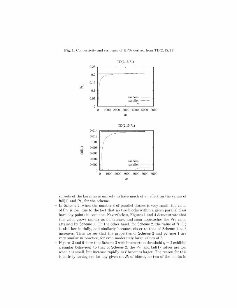
The results of these calculations are presented in graphical form in Figures 1–6. In these figures, we plot the connectivity or resilience of a random scheme anda corresponding deterministic scheme. The solid lines, labelled “random”, referto Scheme 1; the dashed lines, labelled “parallel”, refer to Scheme 2 or Scheme 3.The dotted lines, labelled “σ”, indicate the standard deviation of the valuescomputed for Scheme 1 over the 100 trials (since the standard deviations arequite small, these lines are very close to the bottom of the graphs). The value mis the number of blocks in the associated set system (i.e., the number of nodesin the network).

In the case of Scheme 1, we also computed the maximum and minimum valuesof fail(1) and Pr1 obtained over the 100 trials, for each value of m. As well, wehave tabulated the mean and standard deviation over the 100 samples. In thesetwo tables, the network size is m = `n = 71`. This data is presented, for theschemes derived from a TD(2, 15, 71), in Tables 3 and 4 in the Appendix.

Some of the main observations we can draw from these results are as follows:

– In Figures 1–6, the plots of the values of fail(1) or Pr1 as blocks are selecteduniformly from a TD(2, k, n) or TD(3, k, n) (Scheme 1) are all essentiallya horizontal line, indicating that on average the values of fail(1) and Pr1do not change greatly, even if the number of blocks selected is quite small.This is entirely to be expected: fail(1) and Pr1 by definition are quantitiesthat represent an average over all the keyrings in the network, so taking theaverage over smaller, uniformly selected subsets of keyings should not affectthese values too much. The average values computed in our experiments arein fact very close to the exact average values that are computed theoretically.

– One quantity of particular interest here is the standard deviation of fail(1)and Pr1 for Scheme 1, since this determines the extent to which a particu-lar random choice of subnetwork may have fail(1) or Pr1 values that differfrom the average values for the scheme as a whole. Naturally, the standarddeviation of these values increases slightly when the number blocks is verysmall. However, we can see from Figures 1–6 that these standard deviationsare still extremely low, especially in the case of schemes obtained from thelarger designs. Moreover, there is a very low range of values of fail(1) andPr1 encountered in our experiments. This is evident from Tables 3 and 4in the Appendix, for the schemes derived from a TD(2, 15, 71). Schemes de-rived from other transversal designs exhibit similar behaviour in terms of thevariability of these metrics. Thus we see that in practice, selecting random

Fig. 1. Connectivity and resilience of KPSs derived from TD(2, 15, 71)

0

0.05

0.1

0.15

0.2

0.25

0 1000 2000 3000 4000 5000 6000

Pr1

m

TD(2,15,71)

randomparallel

σ

0

0.002

0.004

0.006

0.008

0.01

0.012

0.014

0 1000 2000 3000 4000 5000 6000

fail(

1)

m

TD(2,15,71)

randomparallel

σ

subsets of the keyrings is unlikely to have much of an effect on the values offail(1) and Pr1 for the scheme.

– In Scheme 2, when the number ` of parallel classes is very small, the valueof Pr1 is low, due to the fact that no two blocks within a given parallel classhave any points in common. Nevertheless, Figures 1 and 4 demonstrate thatthis value grows rapidly as ` increases, and soon approaches the Pr1 valueattained by Scheme 1. On the other hand, for Scheme 2, the value of fail(1)is also low initially, and similarly becomes closer to that of Scheme 1 as `increases. Thus we see that the properties of Scheme 2 and Scheme 1 arevery similar in practice, for even moderately large values of `.

– Figures 3 and 6 show that Scheme 3 with intersection threshold η = 2 exhibitsa similar behaviour to that of Scheme 2: the Pr1 and fail(1) values are lowwhen ` is small, but increase rapidly as ` becomes larger. The reason for thisis entirely analogous: for any given set Bi of blocks, no two of the blocks in

Fig. 2. Connectivity and resilience of KPSs derived from TD(3, 15, 17) with η = 1

0 0.1 0.2 0.3 0.4 0.5 0.6 0.7 0.8 0.9

0 1000 2000 3000 4000 5000

Pr1

m

TD(3,15,17), η=1

randomparallel

σ

0

0.005

0.01

0.015

0.02

0.025

0.03

0.035

0.04

0 1000 2000 3000 4000 5000

fail(

1)

m

TD(3,15,17), η=1

randomparallel

σ

that set intersect in two points, and hence for η = 2 there are no secure linksformed between nodes whose keyrings are derived from such blocks.

– Figures 2 and 5 are interesting, as they show a slightly different behaviourpattern for Scheme 3 in the case of intersection threshold η = 1. Here thePr1 and fail(1) values are in fact higher when ` is small, and then decreasefor larger values of `, eventually approaching the properties of Scheme 1.This is explained by the fact that two blocks within the same set Bi haveprobability k

n+1 of sharing a common key (cf. Table 2), which is higher (for

the parameters under consideration) than the average probability k(2n−k+3)2(n2+n+1)

that two blocks chosen uniformly from a TD(3, k, n) share at least one key.As in previous cases, it is clear from these graphs that once a reasonablenumber of the sets Bi are chosen, the properties of Scheme 3 are very closeto those of Scheme 1.

Fig. 3. Connectivity and resilience of KPSs derived from TD(3, 15, 17) with η = 2

0

0.05

0.1

0.15

0.2

0.25

0.3

0.35

0 1000 2000 3000 4000 5000

Pr1

m

TD(3,15,17), η = 2

randomparallel

σ

0

0.0005

0.001

0.0015

0.002

0.0025

0.003

0.0035

0 1000 2000 3000 4000 5000

fail(

1)

m

TD(3,15,17), η = 2

randomparallel

σ

We conclude that removal of keyrings from a KPS based on transversal de-signs, whether randomly or deterministically as in Scheme 2 or 3, causes noundue disruption to the behaviour of the scheme.

4 An Efficient New Approach to Calculating Connectivityand Resilience for Arbitrary Set Systems

In this section, we describe a new approach to facilitate the efficient evaluationof metrics for connectivity and resilience in general KPSs. We were motivated todo this in order to compute the metrics of our random scheme that consists ofrandom subsets of blocks of a transversal design. Suppose we start with any setsystem (X,A) having blocks of size k. Denote b = |A|. Suppose the maximumintersection of any two blocks in A is t− 1. (In a given application, the value of

Fig. 4. Connectivity and resilience of KPSs derived from TD(2, 25, 157)

0

0.02

0.04

0.06

0.08

0.1

0.12

0.14

0.16

0 5000 10000 15000 20000 25000

Pr1

m

TD(2,25,157)

randomparallel

σ

0

0.001

0.002

0.003

0.004

0.005

0.006

0.007

0 5000 10000 15000 20000 25000

fail(

1)

m

TD(2,25,157)

randomparallel

σ

t may already be known beforehand. However, if it were not already known, itcould be computed as the first step of the process we are about to describe.)

For |C| = i where η ≤ i ≤ t− 1, define λC to be the number of blocks A ∈ Acontaining all the points in C. It will turn out that we can compute Pr1 andfail(1) fairly easily if we know all the λC values. This has at least two desirableconsequences:

1. For various types of “structured” set systems (for example, a partially bal-anced t-design) we know the relevant λC ’s and so we can compute formulasfor Pr1 and fail(1) in a straightforward manner.

2. For an arbitrary “unstructured” set system, we can use this approach tocompute Pr1 efficiently. In a “naive” approach, we would probably examineall pairs of blocks to see which pairs form links, which would already requiretime Θ(b2). However, it is straightforward to tabulate all the relevant λC

Fig. 5. Connectivity and resilience of KPSs derived from TD(3, 25, 29) with η = 1

0 0.1 0.2 0.3 0.4 0.5 0.6 0.7 0.8 0.9

0 5000 10000 15000 20000 25000

Pr1

m

TD(3,25,29), η=1

randomparallel

σ

0

0.005

0.01

0.015

0.02

0.025

0 5000 10000 15000 20000 25000

fail(

1)

m

TD(3,25,29), η=1

randomparallel

σ

values in time Θ(b), and then apply the formulas we derive, in order tocompute Pr1. This will be discussed further in Section 4.3.

4.1 Formulas for Connectivity

For a set of points C with |C| ≥ η, define a C-link to be a set of two nodes {A,B}such that A ∩B = C. The number of C-links is denoted by λ′(C); therefore,

λ′(C) = |{{A,B} : A,B ∈ A, A ∩B = C}|.

The next lemma follows easily from the principle of inclusion-exclusion.

Lemma 1. If |C| = i ≤ t− 1, then

λ′(C) =∑

D⊆X\C,|D|≤t−1−i

(−1)|D|(λC∪D

2

). (1)

Fig. 6. Connectivity and resilience of KPSs derived from TD(3, 25, 29) with η = 2

0

0.05

0.1

0.15

0.2

0.25

0.3

0.35

0 5000 10000 15000 20000 25000

Pr1

m

TD(3,25,29), η = 2

randomparallel

σ

0

0.0002

0.0004

0.0006

0.0008

0.001

0.0012

0 5000 10000 15000 20000 25000

fail(

1)

m

TD(3,25,29), η = 2

randomparallel

σ

In particular, λ′(C) =(λC

2

)if |C| = t− 1.

Define an i-link to be any C-link where |C| = i. For η ≤ i ≤ t − 1, let Lidenote the number of i-links (or course, there are no i-links with i ≥ t). Forη ≤ i ≤ t− 1, it is clear that

Li =∑|C|=i

λ′(C). (2)

The quantity

L =

t−1∑i=η

Li (3)

is the total number of links. From this, it immediately follows that

Pr1 =L(b2

) . (4)

Define

qi =∑|C|=i

(λC2

). (5)

We now provide a useful formula for Li.

Lemma 2. For η ≤ i ≤ t− 1, we have that

Li =

t−1∑j=i

(−1)j−i(j

i

)qj . (6)

Proof. In view of (2), we need to sum (1) over all C with |C| = i. When we do

this, each possible term (−1)|D|(λC∪D

2

)is included in the sum

(|C∪D||C|

)=(|D|+i

i

)times.

For η ≤ i ≤ t− 1, let

ai =

i∑j=η

(−1)i−j(i

j

). (7)

Then we have the following.

Theorem 4.

L =

t−1∑i=η

aiqi, (8)

where the qi’s and ai’s are defined in (5) and (7), respectively.

Proof. We sum the formula (6) as i ranges from η to t− 1. The number of timesqi is included in the sum is easily seen to be equal to ai.

We present some applications of the formula (8) for small values of t and η inTable 2.

Now, applying (8) and (4), we have the following formula for Pr1.

Corollary 1.

Pr1 =

∑t−1i=η aiqi(b2

) . (9)

t η L

2 1 q13 2 q23 1 q1 − q24 3 q34 2 q2 − 2q34 1 q1 − q2 + q35 4 q45 3 q3 − 3q45 2 q2 − 2q3 + 3q45 1 q1 − q2 + q3 − q4

Table 2. Applications of Theorem 4

4.2 Formulas for Resilience

Recall that a C-link is a set of two nodes {A,B} such that A ∩ B = C. Thenumber of C-links is λ′(C) and the number of nodes that break the C-link {A,B}is λC−2. The probability that the C-link {A,B} is broken by the compromise ofa random node not in the link is (λC − 2)/(b− 2). Averaging over all L links, weobtain the following formula for fail(1), which can be viewed as a generalisationof [9, Cor. 4.6]:

fail(1) =1

L

∑{C:η≤|C|≤t−1}

(λC − 2)λ′(C)

b− 2. (10)

In order to compute fail(1) using (10), we first need to evaluate the expression∑λCλ

′(C). Substituting (1) into this sum, we have

∑{C:η≤|C|≤t−1}

λCλ′(C) =

∑{C:η≤|C|≤t−1}

λC ∑D⊆X\C,|D|≤t−1−i

(−1)|D|(λC∪D

2

)=

∑{E:η≤|E|≤t−1}

(λE2

) ∑{C:η≤|C|,C⊆E}

(−1)|E|−|C|λC

,

letting E = C ∪D. As a result, we obtain the following.

Lemma 3. ∑{C:η≤|C|≤t−1}

λCλ′(C) =

∑{E:η≤|E|≤t−1}

µE

(λE2

), (11)

whereµE =

∑{C:η≤|C|,C⊆E}

(−1)|E|−|C|λC . (12)

For future use, we mention a couple of special cases of (12):

µE =

{λE if |E| = η

λE −∑x∈E λE\{x} if |E| = η + 1.

(13)

Next, applying (3) and (2) we have that∑{C:η≤|C|≤t−1}

2λ′(C) = 2L. (14)

Now we can state our main formula.

Theorem 5.

fail(1) =1

L(b− 2)

∑{E:η≤|E|≤t−1}

µE

(λE2

)− 2

b− 2. (15)

Proof. The result follows immediately from (10), (11) and (14).

4.3 Computing Connectivity and Resilience

Suppose we are given a set system (X,A), where b = |A|. As previously men-tioned, we assume that value of the parameter t is already known. Here are thesteps that would be followed to compute Pr1 and fail(1).

1. Compute all the values λC for η ≤ |C| ≤ t− 1. This can be done efficientlyas follows:

(a) Initialise λC ← 0 for all relevant C.

(b) For every block A ∈ A and for every C ⊆ A such that η ≤ |C| ≤ t − 1,set λC ← λC + 1.

(For fixed values of η and t, we observe that the λC ’s can be computed intime Θ(b) by this method.)

2. Compute all the values µC for η ≤ |C| ≤ t− 1, using the formula (12).

3. Compute the values qi for η ≤ i ≤ t− 1, using the formula (5).

4. Compute L using the formula (8).

5. Compute Pr1 = L/(b2

)and compute fail(1) using the formula (15).

Remark: If we only wanted to compute Pr1, then step 2 could be omitted.

4.4 Examples

Here are some small examples to illustrate the application of the formulas wehave developed.

Example 6. Suppose X = {1, . . . , 6} and

A = {{123}, {124}, {125}, {456}, {136}}.

It easy to check that t = 3 in this design. Then we have

λ12 = 3 λ13 = 2 λ14 = 1 λ15 = 1 λ16 = 1 λ23 = 1λ24 = 1 λ25 = 1 λ26 = 0 λ34 = 0 λ35 = 0 λ36 = 1λ45 = 1 λ46 = 1 λ56 = 1λ1 = 4 λ2 = 3 λ3 = 2 λ4 = 2 λ5 = 2 λ6 = 2

It is easy to compute q1 = 13 and q2 = 4. When η = 1, we have L = q1 − q2 = 9and Pr1 = 9/10; when η = 2, we have L = q2 = 4 and Pr1 = 4/10.

In order to compute fail(1), we also need to compute the µC ’s. First, supposeη = 2. Then µC = λC for |C| = 2, and

fail(1) =1

4× 3

(3

(3

2

)+ 2

(2

2

))− 2

3=

1

4.

When η = 1, we need to compute λC when |C| = 1, 2. When |C| = 1, wehave µC = λC . When |C| = 2, we use (13) to compute µC :

µ12 = −4 µ13 = −4 µ14 = −5 µ15 = −5 µ16 = −5 µ23 = −4µ24 = −4 µ25 = −4 µ26 = −5 µ34 = −4 µ35 = −4 µ36 = −3µ45 = −3 µ46 = −3 µ56 = −3

fail(1) =1

9× 3

(4

(4

2

)+ 3

(3

2

)+ 4× 2

(2

2

)− 4

(3

2

)− 4

(2

2

))− 2

3=

7

27.

Here is an example with t = 4. We just compute Pr1 for this example.

Example 7. Suppose X = {1, . . . , 9} and

A = {{1234}, {1235}, {1367}, {5678}, {4789}}.

Here t = 4 and we compute q1 = 14, q2 = 7 and q3 = 1. When η = 1, we haveL = q1 − q2 + q3 = 8 and Pr1 = 4/5; when η = 2, we have L = q2 − 2q3 = 5 andPr1 = 1/2; and when η = 3, we have L = q3 = 1 and Pr1 = 1/10.

5 Conclusion

We have provided two methods of increasing the flexibility of combinatorial keypredistribution schemes. These methods are discussed and evaluated in refer-ence to the transversal design schemes introduced in [5]. The first method is toexploit the underlying structure of transversal designs to explicitly describe awide range of “partial” designs whose properties can easily be analysed usingexisting formulas [9]. The schemes based on these partial designs have propertiesvery similar to the transversal design schemes from which they are derived. The

second method (e.g., see [5]) is to randomly delete blocks from a specified setsystem. We show by running extensive experiments that this method also doesnot affect performance adversely, which contradicts assertions made in [1]. Fi-nally, we develop some new formulas that facilitate the efficient computation ofmetrics of KPS derived from arbitrary set systems. These formulas were usefulin the experiments we carried out, but they may have additional applications inthe theoretical study of combinatorial KPS for wireless sensor networks.

References

1. M. Bose, A. Dey and R. Mukerjee. Key predistribution schemes for distributedsensor networks via block designs. Designs, Codes and Cryptography, 67(1) (2013),111–136.

2. S.A. Camtepe and B. Yener. Key distribution mechanisms for wireless sensor net-works: a survey. Tech. Rep. TR-05-07, Rensselaer Polytechnic Institute (March 2005).

3. J.-W. Dong, D.-Y. Pei and X.-L. Wang. A key predistribution scheme based on3-designs. Lecture Notes in Computer Science 4990 (2008), 81–92 (Inscrypt 2007).

4. L. Eschenauer and V. Gligor. A key-management scheme for distributed sensornetworks. In Proceedings of the 9th ACM Conference on Computer and Communi-cations Security. ACM Press, 2002, pp. 41–47.

5. J. Lee and D.R. Stinson. On the construction of practical key predistributionschemes for distributed sensor networks using combinatorial designs. ACM Trans-actions on Information and System Security, 11(2) (2008), article No. 1, 35 pp.

6. K.M. Martin. On the applicability of combinatorial designs to key predistributionfor wireless sensor networks. Lecture Notes in Computer Science 5557 (2009),124–145 (IWCC 2009).

7. K.M. Martin and M.B. Paterson. An application-oriented framework for wirelesssensor network key establishment. Electron. Notes Theor. Comput. Sci., 192(2)(2008), 31–41.

8. K.M. Martin, M.B. Paterson and D.R. Stinson. Key predistribution for homoge-neous wireless sensor networks with group deployment of nodes. ACM Transactionson Sensor Networks, 7(2) (2010), article No. 11, 27 pp.

9. M.B. Paterson and D.R. Stinson. A unified approach to combinatorial key predis-tribution schemes for sensor networks. Designs, Codes and Cryptography, (OnlineFirst, DOI 10.1007/s10623-012-9749-4).

10. Y. Xiao, V.K. Rayi, B. Sun, X. Du, F. Hu and M. Galloway. A survey of keymanagement schemes in wireless sensor networks. Comput. Commun., 30(11-12)(2007), 2314-2341.

Appendix

Table 3: Resilience of random KPSs derived from TD(2, 15, 71)

` fail(1) (mean) fail(1) (std. dev.) fail(1) (min) fail(1) (max)2 0.013749 0.000642 0.011989 0.0153573 0.013660 0.000381 0.012879 0.0146844 0.013687 0.000278 0.013134 0.0144815 0.013702 0.000234 0.013158 0.0143626 0.013704 0.000179 0.013294 0.0141087 0.013676 0.000140 0.013338 0.0140778 0.013687 0.000136 0.013356 0.0140639 0.013707 0.000109 0.013418 0.013950

10 0.013690 0.000094 0.013476 0.01396411 0.013682 0.000077 0.013505 0.01385012 0.013698 0.000071 0.013552 0.01389713 0.013696 0.000068 0.013517 0.01383614 0.013685 0.000058 0.013558 0.01382015 0.013691 0.000055 0.013528 0.01384116 0.013685 0.000055 0.013586 0.01383017 0.013694 0.000053 0.013583 0.01386218 0.013692 0.000044 0.013579 0.01380019 0.013694 0.000042 0.013602 0.01380820 0.013694 0.000042 0.013582 0.01381221 0.013693 0.000037 0.013588 0.01378022 0.013694 0.000033 0.013602 0.01379223 0.013687 0.000034 0.013603 0.01376024 0.013693 0.000031 0.013632 0.01378025 0.013692 0.000025 0.013614 0.01374626 0.013690 0.000026 0.013592 0.01374927 0.013690 0.000025 0.013631 0.01374328 0.013692 0.000021 0.013630 0.01373729 0.013691 0.000019 0.013633 0.01373030 0.013688 0.000019 0.013639 0.01372931 0.013693 0.000020 0.013655 0.01374932 0.013693 0.000018 0.013645 0.01373233 0.013693 0.000016 0.013661 0.01375234 0.013693 0.000016 0.013659 0.01373735 0.013695 0.000014 0.013667 0.01372436 0.013691 0.000014 0.013655 0.01372737 0.013694 0.000012 0.013664 0.01372538 0.013694 0.000015 0.013664 0.01373539 0.013693 0.000012 0.013662 0.01372640 0.013691 0.000012 0.013668 0.01372041 0.013693 0.000011 0.013668 0.013726

Table 3: Resilience of random KPSs derived from TD(2, 15, 71)(cont).

` fail(1) (mean) fail(1) (std. dev.) fail(1) (min) fail(1) (max)42 0.013695 0.000013 0.013664 0.01372643 0.013693 0.000010 0.013674 0.01372544 0.013693 0.000009 0.013664 0.01371245 0.013692 0.000008 0.013673 0.01371546 0.013694 0.000007 0.013679 0.01371547 0.013693 0.000007 0.013679 0.01370948 0.013693 0.000008 0.013676 0.01371549 0.013693 0.000007 0.013676 0.01371050 0.013693 0.000007 0.013673 0.01371051 0.013694 0.000005 0.013682 0.01370952 0.013693 0.000006 0.013679 0.01370553 0.013694 0.000005 0.013683 0.01370754 0.013694 0.000005 0.013681 0.01370455 0.013694 0.000004 0.013683 0.01370756 0.013693 0.000004 0.013683 0.01370357 0.013693 0.000004 0.013681 0.01370658 0.013693 0.000003 0.013683 0.01370459 0.013693 0.000003 0.013684 0.01369860 0.013693 0.000003 0.013685 0.01370061 0.013693 0.000002 0.013688 0.01369862 0.013693 0.000002 0.013688 0.01370063 0.013693 0.000002 0.013687 0.01370264 0.013693 0.000002 0.013689 0.01369765 0.013693 0.000001 0.013689 0.01369766 0.013693 0.000001 0.013690 0.01369767 0.013693 0.000001 0.013691 0.01369668 0.013693 0.000001 0.013692 0.01369569 0.013693 0.000000 0.013692 0.01369470 0.013693 0.000000 0.013693 0.01369471 0.013693 0.000000 0.013693 0.013693

Table 4: Connectivity of random KPSs derived from TD(2, 15, 71)

` Pr1 (mean) Pr1 (std. dev.) Pr1 (min) Pr1 (max)1 0.208129 0.008217 0.185111 0.2281692 0.208647 0.003964 0.197283 0.2186593 0.208178 0.002706 0.202719 0.2151214 0.208296 0.001944 0.204200 0.2131595 0.208403 0.001608 0.204138 0.2127956 0.208455 0.001297 0.204861 0.2117217 0.208241 0.001010 0.205467 0.210976

Table 4: Connectivity of random KPSs derived from TD(2, 15, 71)(cont).

` Pr1 (mean) Pr1 (std. dev.) Pr1 (min) Pr1 (max)8 0.208214 0.000963 0.205741 0.2109269 0.208424 0.000790 0.206175 0.21035510 0.208313 0.000695 0.206834 0.21037411 0.208234 0.000541 0.206914 0.20940912 0.208359 0.000501 0.207433 0.20976413 0.208359 0.000477 0.207073 0.20941814 0.208284 0.000427 0.207436 0.20933315 0.208332 0.000422 0.207219 0.20951516 0.208267 0.000397 0.207473 0.20933517 0.208340 0.000391 0.207518 0.20934118 0.208324 0.000329 0.207455 0.20910519 0.208339 0.000311 0.207681 0.20910920 0.208333 0.000309 0.207523 0.20926721 0.208333 0.000277 0.207566 0.20900722 0.208340 0.000243 0.207638 0.20906423 0.208282 0.000248 0.207686 0.20877524 0.208336 0.000230 0.207860 0.20899925 0.208327 0.000184 0.207737 0.20874426 0.208307 0.000198 0.207572 0.20876327 0.208309 0.000186 0.207903 0.20870628 0.208322 0.000160 0.207863 0.20864829 0.208314 0.000145 0.207887 0.20859530 0.208295 0.000146 0.207896 0.20861831 0.208337 0.000148 0.208046 0.20876032 0.208330 0.000136 0.207953 0.20862033 0.208334 0.000125 0.208096 0.20879934 0.208331 0.000122 0.208052 0.20868535 0.208344 0.000109 0.208120 0.20856036 0.208318 0.000109 0.208046 0.20862137 0.208338 0.000094 0.208113 0.20858838 0.208338 0.000114 0.208114 0.20865539 0.208330 0.000089 0.208108 0.20856840 0.208316 0.000091 0.208140 0.20855641 0.208336 0.000086 0.208144 0.20856942 0.208345 0.000098 0.208104 0.20856943 0.208331 0.000074 0.208187 0.20858544 0.208334 0.000065 0.208109 0.20848045 0.208328 0.000060 0.208179 0.20849246 0.208335 0.000053 0.208232 0.20849947 0.208334 0.000053 0.208223 0.20845848 0.208331 0.000058 0.208205 0.20849949 0.208330 0.000050 0.208211 0.208460

Table 4: Connectivity of random KPSs derived from TD(2, 15, 71)(cont).

` Pr1 (mean) Pr1 (std. dev.) Pr1 (min) Pr1 (max)50 0.208332 0.000051 0.208178 0.20845951 0.208339 0.000041 0.208246 0.20845752 0.208332 0.000042 0.208226 0.20842653 0.208338 0.000034 0.208256 0.20844054 0.208339 0.000036 0.208245 0.20841855 0.208336 0.000033 0.208255 0.20843756 0.208333 0.000030 0.208256 0.20841057 0.208334 0.000028 0.208241 0.20842758 0.208329 0.000026 0.208255 0.20841759 0.208331 0.000023 0.208262 0.20837160 0.208332 0.000021 0.208273 0.20838661 0.208333 0.000017 0.208295 0.20837162 0.208335 0.000017 0.208291 0.20838763 0.208334 0.000016 0.208285 0.20839764 0.208332 0.000012 0.208301 0.20836165 0.208332 0.000010 0.208305 0.20836066 0.208332 0.000009 0.208312 0.20836067 0.208333 0.000007 0.208316 0.20835868 0.208334 0.000005 0.208321 0.20834769 0.208333 0.000003 0.208324 0.20834370 0.208333 0.000002 0.208329 0.20833971 0.208333 0.000000 0.208333 0.208333