Pedro Negrete-Regagnon Vol. 13, No. 7/July 1996/J. Opt. Soc. Am. A 1557 Practical aspects of image recovery by means of the bispectrum Pedro Negrete-Regagnon* Applied Optics, Blackett Laboratory, Imperial College, London SW7 2BZ, UK Received October 2, 1995; accepted January 11, 1996 The use of the bispectrum as a tool to handle the phase-retrieval problem associated with speckle interfer- ometry is examined. The basic concepts and equations involved in bispectral imaging are discussed. Based in signal-to-noise ratio considerations, a simple recipe to predict the success of bispectral imaging is given. Because of their higher noise tolerance, two least-squares minimization schemes are used to reconstruct the object Fourier phase encrypted in the bispectral phase. The error-reduction algorithm for phase retrieval is applied in conjunction with the minimization procedures to overcome stagnation at local minima. Ex- amples with simulated and real astronomical data are presented, including a comparison of the outcome of bispectral processing applied to both adaptively compensated and uncompensated data. The resulting diffraction-limited reconstructions are very similar. 1996 Optical Society of America 1. INTRODUCTION High-resolution ground-based astronomical imaging in the visible region of the spectrum has always represented a challenge for astronomers. Most efforts have been con- centrated in two directions: the application of so-called postprocessing speckle-based techniques and, more re- cently, the development and implementation of adaptive optics (AO) and laser beacon technologies. This paper is related to the former subject, and in it the use of a high-order statistical tool, the bispectrum, is examined as a complementary technique to speckle interferometry aimed at obtaining approximate diffraction-limited im- ages from ground-based telescopes. The postprocessing imaging methods originated in 1970 when Labeyrie recognized the higher-frequency con- tent present in short-exposure images. 1 He invented a technique called speckle interferometry that is based on the collection of many such short-exposure images and their subsequent processing. Speckle interferome- try estimates the spatial energy spectrum of an object as the ensemble average of the individual energy spectra of many short-exposure images. The ensemble average of the short-exposure images leads directly to the long- exposure counterpart. This is equivalent to averaging their Fourier amplitudes, which vary widely, and results in an average of zero, suppressing the high-frequency information. Inasmuch as the energy spectrum is the square of the Fourier amplitude, it is always a posi- tive quantity, resulting in an ensemble average that is different from 0. The technique requires simultaneous measurements of an unresolved (pointlike) star for esti- mation of the atmosphere–telescope point-spread func- tion (normally the reference measurements are taken from a nearby star immediately before or after the object, assuming that seeing conditions remain the same). A simple deconvolution procedure is then enough to per- mit one to estimate the object’s energy spectrum (and hence its Fourier modulus) or the object’s autocorrelation (the object’s spatial energy spectrum and object autocor- relation are Fourier transforms of each other). The auto- correlation contains most of the desired information for simple objects, but analysis of complicated objects re- quires image reconstruction, which necessitates Fourier phase recovery. 2 Complementary algorithms were pro- posed in 1974 (Knox and Thompson 3 ) and in 1977 (speckle masking or triple correlation 4 ) to allow the object phase to be reconstructed from speckle measurements. The application of these algorithms, aimed at obtaining diffraction-limited images from speckle data, is termed speckle imaging. In recent years there has been an increase of inter- est in the development of novel speckle-based techniques such as phase-diversity speckle imaging, which is a blend of two concepts: speckle imaging and phase diversity. Phase diversity requires the simultaneous collection of fo- cused and defocused speckle images. The goal is to iden- tify an object that is consistent with both collected images, given the known defocus or phase diversity. 5 Among other new techniques, blind deconvolution (or multiframe blind deconvolution) stands out. 6 Again a deconvolution procedure is needed, but in this case both the object and the point-spread function (PSF) must be recovered from the blurred, noisy data. In practice, all the techniques mentioned above pro- duce satisfactory results when the incoming photon flux is high. Unfortunately, most interesting astro- nomical objects are too faint to produce a significant number of detected photons during the short exposure times required by those methods. At low-light-level con- ditions it seems that speckle imaging techniques are probably the only practical method for obtaining approxi- mated diffraction-limited images. It is now commonly accepted that the algorithms used to extract the object Fourier phase from a series of speckle frames, namely, the Knox– Thompson algorithm and the triple correla- tion or bispectrum, are from the same family or high- order spectra. Several authors have recognized that the Knox – Thompson algorithm is only a subset or special case from the more complete bispectrum and that the 0740-3232/96/071557-20$10.00 1996 Optical Society of America
Transcript
Pedro Negrete-Regagnon Vol. 13, No. 7 /July 1996/J. Opt. Soc. Am. A 1557
Practical aspects of image recoveryby means of the bispectrum
Pedro Negrete-Regagnon*
Applied Optics, Blackett Laboratory, Imperial College, London SW7 2BZ, UK
Received October 2, 1995; accepted January 11, 1996
The use of the bispectrum as a tool to handle the phase-retrieval problem associated with speckle interfer-ometry is examined. The basic concepts and equations involved in bispectral imaging are discussed. Basedin signal-to-noise ratio considerations, a simple recipe to predict the success of bispectral imaging is given.Because of their higher noise tolerance, two least-squares minimization schemes are used to reconstruct theobject Fourier phase encrypted in the bispectral phase. The error-reduction algorithm for phase retrievalis applied in conjunction with the minimization procedures to overcome stagnation at local minima. Ex-amples with simulated and real astronomical data are presented, including a comparison of the outcomeof bispectral processing applied to both adaptively compensated and uncompensated data. The resultingdiffraction-limited reconstructions are very similar. 1996 Optical Society of America
1. INTRODUCTION
High-resolution ground-based astronomical imaging inthe visible region of the spectrum has always representeda challenge for astronomers. Most efforts have been con-centrated in two directions: the application of so-calledpostprocessing speckle-based techniques and, more re-cently, the development and implementation of adaptiveoptics (AO) and laser beacon technologies. This paperis related to the former subject, and in it the use of ahigh-order statistical tool, the bispectrum, is examinedas a complementary technique to speckle interferometryaimed at obtaining approximate diffraction-limited im-ages from ground-based telescopes.
The postprocessing imaging methods originated in1970 when Labeyrie recognized the higher-frequency con-tent present in short-exposure images.1 He inventeda technique called speckle interferometry that is basedon the collection of many such short-exposure imagesand their subsequent processing. Speckle interferome-try estimates the spatial energy spectrum of an objectas the ensemble average of the individual energy spectraof many short-exposure images. The ensemble averageof the short-exposure images leads directly to the long-exposure counterpart. This is equivalent to averagingtheir Fourier amplitudes, which vary widely, and resultsin an average of zero, suppressing the high-frequencyinformation. Inasmuch as the energy spectrum is thesquare of the Fourier amplitude, it is always a posi-tive quantity, resulting in an ensemble average that isdifferent from 0. The technique requires simultaneousmeasurements of an unresolved (pointlike) star for esti-mation of the atmosphere–telescope point-spread func-tion (normally the reference measurements are takenfrom a nearby star immediately before or after the object,assuming that seeing conditions remain the same). Asimple deconvolution procedure is then enough to per-mit one to estimate the object’s energy spectrum (andhence its Fourier modulus) or the object’s autocorrelation(the object’s spatial energy spectrum and object autocor-
0740-3232/96/071557-20$10.00
relation are Fourier transforms of each other). The auto-correlation contains most of the desired information forsimple objects, but analysis of complicated objects re-quires image reconstruction, which necessitates Fourierphase recovery.2 Complementary algorithms were pro-posed in 1974 (Knox and Thompson3) and in 1977 (specklemasking or triple correlation4) to allow the object phaseto be reconstructed from speckle measurements. Theapplication of these algorithms, aimed at obtainingdiffraction-limited images from speckle data, is termedspeckle imaging.
In recent years there has been an increase of inter-est in the development of novel speckle-based techniquessuch as phase-diversity speckle imaging, which is a blendof two concepts: speckle imaging and phase diversity.Phase diversity requires the simultaneous collection of fo-cused and defocused speckle images. The goal is to iden-tify an object that is consistent with both collected images,given the known defocus or phase diversity.5 Amongother new techniques, blind deconvolution (or multiframeblind deconvolution) stands out.6 Again a deconvolutionprocedure is needed, but in this case both the object andthe point-spread function (PSF) must be recovered fromthe blurred, noisy data.
In practice, all the techniques mentioned above pro-duce satisfactory results when the incoming photonflux is high. Unfortunately, most interesting astro-nomical objects are too faint to produce a significantnumber of detected photons during the short exposuretimes required by those methods. At low-light-level con-ditions it seems that speckle imaging techniques areprobably the only practical method for obtaining approxi-mated diffraction-limited images. It is now commonlyaccepted that the algorithms used to extract the objectFourier phase from a series of speckle frames, namely,the Knox–Thompson algorithm and the triple correla-tion or bispectrum, are from the same family or high-order spectra. Several authors have recognized that theKnox–Thompson algorithm is only a subset or specialcase from the more complete bispectrum and that the
1996 Optical Society of America
1558 J. Opt. Soc. Am. A/Vol. 13, No. 7/July 1996 Pedro Negrete-Regagnon
use of the latter yields slightly better results.7,8 Themain results with the triple correlation or bispectraltechnique, originally called speckle masking, are dueto the group of researchers led by Weigelt.4,9,10 Theyhave reconstructed impressive images of star clustersand other difficult to image astronomical objects.11,12 Al-though the diffraction limit has been attained for suchsimple objects (resolved stars, binary stars, and starclusters), speckle imaging is still not widely used as animaging tool.
The purpose of this paper is to examine in some de-tail the use of the bispectrum as such an imaging tool.It comprises the information of several scattered refer-ences in an attempt to lower the entry barrier of the tech-nique not only to astronomers but to scientists workingin other disciplines. It also analyzes the strengths andweaknesses of the method and provides a simple recipe forestimating whether bispectral imaging will be successfulat producing the desired diffraction-limited image underparticular observing conditions. The approaches to re-constructing the object’s Fourier phase from the bispec-tral phase are based on least-squares minimizations, incontrast to the recursive scheme traditionally employedin the studies reported in Refs. 9 and 10. I have as-sessed the reliability of the algorithms and the code byprocessing both carefully simulated data and real data(including a brief comparison of the outcome of bispec-tral processing applied to adaptively compensated anduncompensated data).
The material in the paper is presented in nine sections.Section 2 introduces the simulation of speckle data usedto test the algorithms. Section 3 reviews the standardspeckle interferometry method of estimating the object’sFourier modulus, together with expressions for its signal-to-noise ratio (SNR). Based on SNR considerations,Section 4 discusses the performance of speckle interfero-metry, and hence of the whole speckle imaging methodol-ogy, and establishes a simple recipe for estimation of theminimum requirements to guarantee satisfactory results.Section 5 deals with the theory behind the bispectralmethod, its SNR, and some practical details about itsevaluation. A phase-recovery strategy based on mini-mization schemes is presented in Section 6, and a briefdiscussion of the effect of the application of a window func-tion for a final image reconstruction is given in Section 7.Examples of bispectral processing with both simulatedand real data are presented in Section 8. Finally, a sum-mary of bispectral imaging in the form of a block diagramand some conclusions are presented in Sections 9 and 10,respectively.
2. SPECKLE DATA SIMULATIONThe image isx, yd resulting from an object osx, yd beingimaged by the atmosphere–telescope system can be de-scribed by the convolution
isx, yd ZZ `
2`
osx0, y 0 dhsx0 2 x, y 0 2 yddx0dy 0, (1)
where hsx, yd is the intensity PSF and represents theimage formed by the system with the object consideredas a point source. The Fourier spectrum for the imageis given by
I su, vd Osu, vdH su, vd , (2)
where I su, vd, Osu, vd, and Hsu, vd are the Fourier trans-forms of isx, yd, osx, yd, and hsx, yd, respectively. InFourier space the frequency components of the objectare weighted by the normalized optical transfer function(OTF) H su, vd, given by13
H su, vd
ZZ `
2`
P sx, ydPpsx 2 ulR, y 2 vlRddxdyZZ `
2`
jP sx, ydj2dxdy
,
(3)
where P sx, yd defines a combined atmosphere–telescopepupil function. To simulate a short-exposure image froma given object, the system OTF needs to be evaluatedfor a particular realization of the atmosphere–telescopepupil function P sx, yd. This pupil function is given asthe product of two terms,
P sx, yd PT sx, ydAsx, yd . (4)
The first one, PT sx, yd, is fixed and represents the tele-scope’s pupil function and aberrations that are due to theoptics:
PT sx, yd
8>><>>: jPT sx, ydjexp
"2p
liW sx, yd
#inside the pupil
0 otherwise
,
(5)
where W sx, yd represents the deformation of a wave frontin the exit pupil relative to a reference sphere centered onthe intersection of the image plane and the optical axis.The second term of Eq. (4), Asx, yd, is variable from frameto frame and represents the random effects on amplitudeand phase that are due to atmospheric turbulence13:
Asx, yd jAsx, ydjexpfifAsx, ydg , (6)
where the modulus jAsx, ydj represents the degree of sup-pression of the amplitude of the incoming optical waveand the phase distribution fAsx, yd describes the wave-front phase distortions. Amplitude fluctuations (scintil-lation) are responsible for the well-known phenomenon ofstar twinkling and can be regarded as a random apodiza-tion of the telescope pupil (for a review on scintillationphenomena see Ref. 14). It is commonly accepted thatthe phase variations that are due to atmospheric tur-bulence follow Kolmogorov statistics,13 and the effectsof these inhomogeneities are simulated by use of a sin-gle phase screen at the telescope pupil plane. The pro-cedure used to simulate a phase screen containing theKolmogorov power spectrum is described in Appendix A.
In practice the OTF is calculated as the normalized au-tocorrelation of P sx, yd [Eq. (4)]. This involves the tele-scope’s pupil function and one Kolmogorov phase screenrepresenting the frozen atmosphere. Fixed aberrationsand amplitude fluctuations (scintillation) are normally ig-nored but can easily being included in the simulation.The desired real-valued short-exposure image is simply
Pedro Negrete-Regagnon Vol. 13, No. 7 /July 1996/J. Opt. Soc. Am. A 1559
Fig. 1. Low-light-level image generation.
formed as the inverse Fourier transform of the productbetween the OTF and the Fourier transform of the object.
The procedure mentioned above applies to brightsources (high light level), but most interesting astro-nomical objects are generally faint, and only few hundredphotons are detected in short-exposure frames. To gen-erate low-light-level images, one must control the numberof photons detected per frame. Figure 1 illustrates thephoton-limited simulation. The normalized cumulativesum of the high-light-level frame is regarded as a sin-gle column. This can be interpreted as the probability-distribution function for incoming photons (or, moreproperly, photoevents). One uses a uniformly distributedrandom number between 0 and 1, representing one photo-event, as the ordinate in the distribution function to findthe abscissa. This abscissa is the index number assignedto the pixel collecting the photon, and one unit is given forthat pixel. The process is repeated several times untilthe required number of photons per frame, K, is reached.One forms the low-light-level image by rearranging thepixels and their new values.
As an example, Fig. 2 shows the diffraction-limited im-age of one test object: a binary object with extendedcomponents. Also shown in Fig. 2 are one high-lightshort-exposure image, the long-exposure image formed bythe average of 1000 of such short-exposure frames, and ashort-exposure image formed by 5000 photons. For thiscase a turbulence level of Dyr0 20 is assumed, where Dis the telescope diameter and r0 is the Fried parameter.
3. ENERGY SPECTRUM ESTIMATIONThe relation between the object osx, yd and the imageisx, yd formed by the incoherent atmosphere–telescopesystem is expressed in the Fourier domain by Eq. (2).Given a set of N short-exposure images insx, yd, the en-semble average
kInsu, vdl Osu, vdkHnsu, vdl (7)
leads to the Fourier spectrum of the long-exposure image.This ensemble-averaging operation suppresses high-frequency response. Following Labeyrie’s ideas,1 onecan retain the high-frequency information if the ensem-ble average is performed over the energy spectra set,namely, the squared modulus of the Fourier transformof each frame:
kjInsu, vdj2l jOsu, vdj2kjHnsu, vdj2l . (8)
In this case, large variations at high frequencies of thesquared modulation transfer function (MTF) jHnsu, vdj2are always positive quantities, giving an average differentfrom zero.
To have the desired estimate for the object’s Fouriermodulus jOsu, vdj, one must know the average squaredMTF for the system. One normally does this by takinga similar series of short-exposure images on an unresolv-able star (reference star) that is near the object of interestand obtaining the same ensemble average of energy spec-tra. Because the reference star acts as a point source,the ensemble-averaged energy spectrum of the image isalso the ensemble-averaged squared MTF:
kjInref su, vdj2l kjHnsu, vdj2l . (9)
If the reference star is imaged immediately after or beforethe object of interest, it is possible to assume that theseeing conditions are the same for both measurements.The object’s Fourier modulus is then simply given by
jOsu, vdj
"kjInsu, vdj2l
kjHnsu, vdj2l 1 e
# 1/2
"kjInsu, vdj2l
kjInref su, vdj2l 1 e
# 1/2
, (10)
where e is a parameter chosen to prevent division by 0and is of the order of the machine precision used. Onestill requires a further windowing procedure to avoidthe contribution from noisy frequencies outside the tele-scope diffraction limit. This is discussed in more detailin Section 7.
Although the above procedure seems straightforward,the low light levels involved require some considerationof the SNR in estimation of the energy spectrum.
Fig. 2. Simulated extended object at a high light level. Thelong-exposure image (c) is the average over 1000 short-exposureframes.
1560 J. Opt. Soc. Am. A/Vol. 13, No. 7/July 1996 Pedro Negrete-Regagnon
A. Energy Spectrum Signal-to-Noise RatioIn speckle interferometry a fundamental limitation arisesin the finite number of measured photoevents (particu-larly for the faint objects of interest in astronomy).Several papers13,15,16 address the quality of the statis-tical estimates in such photon-limited conditions. Inthis section only the main results related to the qualityof the energy spectrum estimation are presented.
The quality of a statistical estimator is typically char-acterized by a SNR. The SNR is defined as13,17
SNR mean or expected value of quantity
standard deviation of quantity. (11)
To obtain an expression for the expected single-frameSNR in the energy spectrum, we model the measuredimage13 as
dnsx, yd KnP
k1dsx 2 xk , y 2 ykd , (12)
where dnsx, yd represents the two-dimensional detectedsignal (the nth frame), dsx 2 xk, y 2 ykd represents thekth photoevent occurring at sxk, ykd, and Kn is the numberof photoevents in the image. The Fourier transform ofthe detected image, Dnsx, yd, is given by
Dnsu, vd ZZ `
2`
dnsx, ydexpf2i2psux 1 vydgdxdy
KnX
k1
expf2i2psuxk 1 vykdg . (13)
The most obvious estimator for the energy spectrum of aset of photon-limited images, kjDnsu, vdj2l, is biased by theaverage number of photons per frame (Ref. 13, p. 516):
kjDnsu, vdj2l K2
1 K2kjInsu, vdj2l , (14)
where the circumflex denotes normalization skIns0, 0dj2l 1d. Dainty and Greenaway15 defined an unbiased esti-mator as
Qnsu, vd jDnsu, vdj2 2 Kn . (15)
If we consider only frequencies higher than one half ofthe diffraction-limited cutoff frequency, the expression forthe single-frame SNR was calculated with this unbiasedestimator as15
SNR1su, vd kQnsu, vdlsQ su, vd
KkjInsu, vdj2l
1 1 KkjInsu, vdj2l
K jOsu, vdj2kjHnsu, vdj2l
1 1 KjOsu, vdj2kjHnsu, vdj2l. (16)
According to Ref. 15, we can approximate Eq. (16) by con-sidering two levels in the incoming photon flux:
1. For bright objects,
SNR1su, vd ø 1 ; (17)
2. For faint objects,
SNR1su, vd ø kHosu, vdjOsu, vdj2, (18)
where k Kyns is the average number of photons perspeckle [ns is the number of speckles per frame, definedin Ref. 15 as ns sDyr0d2y0.435] and H0su, vd is the nor-malized, diffraction-limited, and aberration-free OTF ofthe telescope.
It was noted recently16,18 that in AO-compensated sys-tems the compensated OTF, Hcsu, vd, is still random,but it can no longer be modeled as a circularly complexGaussian random process because the real and the imagi-nary parts of Hnsu, vd have unequal variances. Rather,the compensated OTF is better modeled as a more gen-eral case of a complex-valued random process. A morecomplicated expression than Eq. (16) for the single-frameSNR in the compensated case can be found in Ref. 16.As a result, the single-frame SNR for compensated im-ages can be larger than unity at higher frequencies thanfor the uncompensated case. The accuracy of the sta-tistical model for the modulus of the partially or totallycompensated OTF has been evaluated by comparison ofthe energy-spectrum SNR estimate obtained from simula-tion with the one predicted by the theoretical expression.The results are in close agreement.16 The model has alsobeen validated with experimental data,18 but the resultsare not definitive, mainly because of the suboptimal AOsystem used.
When measurement noise is present in an image-detection system, such as in a CCD readout device, theenergy spectrum SNR is further reduced. Read noisein CCD readout devices is generally modeled as additivezero-mean white Gaussian noise with standard deviationsrn, typically given in electrons or photoevents per pixel.CCD read noise is also modeled as being statistically in-dependent of the random process that provides the signalphotons. In this case the estimator of the image energyspectrum is also biased by a read-noise-dependent termgiven by P srn
2, where P is the number of pixels in theimage.18
In practice (from both AO-compensated and uncompen-sated systems), one can evaluate the single-frame SNRfrom a finite data set by averaging a finite number of re-alizations of the bias-removed energy spectrum of manyindividual frames. The single-frame unbiased estimatefor the energy spectrum obtained from the nth frameis
Qnsu, vd jDnsu, vdj2 2 Kn 2 P srn2, (19)
where Dnsu, vd is the Fourier transform of the nth frameand Kn is the actual number of detected photoevents inthat frame. The estimate of Q obtained from a finitedata set containing N frames is
QN su, vd kQnsu, vdlN 1N
NXn1
Qnsu, vd , (20)
and the SNR is then
Pedro Negrete-Regagnon Vol. 13, No. 7 /July 1996/J. Opt. Soc. Am. A 1561
SNR1su, vd
QN su, vd
hvarfQnsu, vdgj1/2
kQnsu, vdlN
hkfQnsu, vdg2lN 2 fkQnsu, vdlN g2j1/2
1N
NXn1
Qnsu, vd(1N
NXn1
fQnsu, vdg2 2
"1N
NXn1
Qnsu, vd
# 2) 1/2.
(21)
We improve the energy-spectrum SNR by averaging theenergy spectra from many realizations of the image. Theresulting SNR is
SNRN su, vd p
N 3 SNR1su, vd , (22)
where N is the number of frames averaged. Improve-ments in the energy-spectrum SNR resulting fromAO-compensated data mean that one must process fewercompensated frames to achieve a predetermined SNR.
4. PERFORMANCE OF SPECKLE IMAGINGTo understand the performance of speckle imaging atlow light levels, and hence the quality of reconstructedimages, consider the energy spectrum SNR obtained fromN short-exposure frames [relation (18) and Eq. (22)]:
SNRN su, vd øp
N kH0su, vdjOsu, vdj2 . (23)
Relation (23) shows that SNRN su, vd closely follows thenormalized distortion-free object energy spectrum. Thisdependence results in a limited number of spectral com-ponents at frequencies su, vd having SNRN above unity.The rest of the frequencies do not have enough signal,and SNRN lies below the threshold of unity imposed byphoton noise. To illustrate this, Fig. 3(a) shows a plot ofthe energy spectrum SNRN obtained from the simulateddata set described in Section 2; the threshold at SNRN ø 1is clearly visible. For comparison, we evaluated the ap-proximated SNRN associated with the original object spec-tral components by using relation (23), and it is shown inFig. 3(b).
The noise in the integrated spectrum [Fig. 3(a)] mani-fests itself as white noise. The noise level is equal to asignal that has a SNR of 1. From relation (23),
Noise level ø1
kp
N
ns
Kp
N
2.3K
pN
√Dr0
! 2
. (24)
The noise level calculation given by relation (24) predictsthe limiting noise that affects speckle data. This noiselevel is due to the quantum nature of light and dependsonly on the detected light level, the number of frames,and the atmospheric conditions; the noise level in speckleimaging is independent of the object.
It is known that information can be obtained fromthe spatial energy spectrum for lower SNR values be-cause the autocorrelation, which is the Fourier transformof the energy spectrum, combines signal coherently and
noise incoherently; thus the noise can be averaged out tosome extent.8 In the case of imaging, the structure incomplicated images is determined primarily from phaseinformation.19 Unfortunately, phase values become use-less below a SNR of ,1 because of the 2p ambiguity of thephase. Image reconstruction is then limited to those spa-tial frequencies for which relation (23) prescribes a SNRgreater than unity.
Binary and other pointlike objects display a dramaticthreshold effect because the objects are so simple. Thedesired information is either present or not (see, for in-stance, the SNR measurements from the binary starb Del in Subsection 8.B.2). Because the spectra of bi-nary objects are relatively simple (fringes) with largesignals at high frequencies, it is possible to obtain high-precision results. Because of this, the most productivearea in speckle interferometry has been investigation ofbinary star and star clusters (see Refs. 20–22).
The signals of more-complicated objects also experiencethe threshold effect mentioned above, but the transition isnot usually so dramatic, as a complicated object has sev-eral levels of information associated with it [see Fig. 3(b)].The fact that the signal from an extended object has aSNR , 1 for most of its frequencies can be serious draw-back for any speckle imaging technique.
Fig. 3. Energy-spectrum SNR from a simulated speckle dataset. The parameters used for the simulation are Dyr0 20,N 5000, and K 1500 (standard deviation sK 50). TheSNR without photon noise shown in (b) was evaluated from theoriginal object’s energy spectrum and by use of relation (23).The profiles in (c) were taken in the direction indicated by thearrow in (a). As is clear from (b) and (c), the speckle dataset does not have enough signal to permit estimation of mostof the spectral components associated with the object. Imagereconstruction will be limited to those spatial frequencies thatshow SNR’s greater than unity in (a).
1562 J. Opt. Soc. Am. A/Vol. 13, No. 7/July 1996 Pedro Negrete-Regagnon
5. BISPECTRUM ESTIMATIONAlthough the method of speckle interferometry offers thepossibility of extracting object information not retriev-able from a single image, this information is generallyincomplete: the object phase is lost. The problem ofreconstructing the unknown object phase has been thesubject of much research. Attempts to form images fromspeckle data by use of correlation techniques began withthe Knox–Thompson algorithm3 and were later generali-zed by Weigelt10 in a method that used the triple correla-tion (TC) or its Fourier transform, the bispectrum.7,9,10,23
In this section the use of this high-order bispectrum tohandle the phase-retrieval problem is described.
The triple correlation of a two-dimensional objectosx, yd is defined by
oTCsx1, y1, x2, y2d ZZ `
2`
opsx, ydosx 1 x1, y 1 y1d
3 osx 1 x2, y 1 y2ddxdy , (25)
and its Fourier transform, the bispectrum, by
O s3dsu1, v1, u2, v2d Osu1, v1dOsu2, v2d
3 Opsu1 1 u2, v1 1 v2d
jO s3dsu1, v1, u2, v2dj
3 expfibsu1, v1, u2, v2dg . (26)
In a way analogous to that by which the average energyspectrum of the speckle data set is calculated,8 it can beshown that the average bispectrum of the image data isrelated to the object bispectrum, a deterministic quantity,by
kI s3dn su1, v1, u2, v2dl O s3dsu1, v1, u2, v2d
3 kT s3dn su1, v1, u2, v2dl , (27)
where kT s3dn su1, v1, u2, v2dl is known as the bispectral
transfer function. Lohmann et al.9 proved that thisbispectral transfer function also transmits informationin frequencies until the telescope diffraction limit. Animportant characteristic of kT s3d
n su1, v1, u2, v2dl is that itis real valued (its phase is effectively 0),24 yielding theresult that the phase of the average bispectrum of theimage equals the bispectral phase bsu1, v1, u2, v2d ofthe object. The relation between the bispectrum phase b
and the object phase f is given by
bsu1, v1, u2, v2d fsu1, v1d 1 fsu2, v2d
2 fsu1 1 u2, v1 1 v2d . (28)
Equation (28) represents a relatively simple relation, andmethods for reconstructing the object phase from thebispectral phase are discussed below (Subsection 6.B).Before that, the effect of photon-limited data on the bis-pectrum estimates and its SNR is discussed.
A. Bispectrum Evaluation at Low Light LevelsEven when there is no need to compensate for thebispectral transfer function during the phase-recoveryprocedure, at low light levels the photon noise in the de-tected images causes an undesired, frequency-dependentphoton bias. Using the same model for the measured
intensity [Eq. (12)] as in the energy-spectrum estimationof photon-limited images (Subsection 3.A), Wirnitzer24
showed that the average bispectrum of the raw speckledata kD s3d
n su1, u2, v1, v2dl is given by
kD s3dn su1, v1, u2, v2dl K 1 K
2fkjInsu1, v1dj2l
1 kjInsu1, v2dj2l
1 kjIpn su1, v1, u2, v2dj2lg
1 K3kI s3d
n su1, v1, u2, v2dl , (29)
where kjInsu, vdj2l and kI s3dn su1, v1, u2, v2dl are the normali-
zed spectral density and bispectrum of the classical im-age intensity, respectively. For high light levels sK ! `dthe term K
3kI s3dn su1, v1, u2, v2dl dominates, and the bis-
pectrum of the detected image is identical to the bispec-trum of the intensity distribution at the detector. Assuggested in Ref. 24, either of two ways to evaluate anunbiased bispectral estimate can be used: (1) apply theresult for the spectral density of a photon-limited image[Eq. (14)] and compensate for the bias term in the bispec-trum [Eq. (29)] or (2) evaluate from the raw data dnsx, yda new quantity,
Q s3dn su1, v1, u2, v2d D s3d
n su1, v1, u2, v2d
2 fjDnsu1, v1dj2 1 jDnsu2, v2dj2
1 jDpn su1 1 u2, v1 1 v2dj2 2 2Kng .
(30)
The expected value of this new estimate is given by
kQ s3dn su1, v2, u2, v2dl K
3kI s3dn su1, v1, u2, v2dl . (31)
The result is therefore an unbiased estimate of the bis-pectrum of isx, yd, although the initial data were photonlimited.
B. Bispectrum Signal-to-Noise RatioThe single-frame SNR for bispectrum analysis when theunbiased estimator Q s3d is used is given by
SNRs3d1 su1, v1, u2, v2d
kQ s3dn su1, v1, u2, v2dl
sQ s3d
, (32)
where sQs3d denotes the standard deviation of the quan-tity Q s3d
n . The derivation of expressions for sQs3d andSNRs3d
1 is a lengthy one and is given in detail in App. Aof Ref. 24. As in the SNR of energy-spectrum estimates[Subsection 3.A), the results for the bispectrum’s SNR canbe summarized for two cases:
1. For bright objects,
SNRs3d1 su1, v1, u2, v2d ø 1 ; (33)
2. For faint objects,
SNRs3d1 su1, v1, u2, v2d ø k
3/2T s3d
0 su1, v1, u2, v2d
3 O s3dsu1, v1, u2, v2d , (34)
where T s3d0 is the normalized, diffraction-limited, and
aberration-free bispectral transfer function (App. B ofRef. 9). From these results Wirnitzer24 concluded that
Pedro Negrete-Regagnon Vol. 13, No. 7 /July 1996/J. Opt. Soc. Am. A 1563
Fig. 4. Perpendicular component of a complex signal.
image reconstruction from the bispectrum is possible inall the cases in which the speckle interferometry processis successful.
Because the object’s Fourier modulus is estimated withrelative ease from the average energy spectrum by tra-ditional speckle interferometry techniques [Eq. (10)], theapplication of the bispectrum is usually limited to thephase-estimation problem. As far as this phase-recoveryproblem is concerned, the SNR measurements of Eq. (32)that use the total bispectral variance sI s3d 2 sR
2 1 sI2
(where sR2 and sI
2 are the variances of the real and theimaginary parts, respectively) are not entirely appropri-ate, as that SNR is relatively insensitive to the individualfluctuations of the real and the imaginary parts of the sig-nal. One can obtain a more reliable estimate of the SNRin the phase of a complex signal by considering the vari-ance of the signal in a direction perpendicular to the meansignal.7,25 An expression for this SNR is now derived.
If R is the real component and I is the imaginarycomponent of a single realization of the complex signal S(see Fig. 4), then the component Sp perpendicular to themean signal kSl is given, by rotation of coordinates, as
Sp I cos b 2 R sin b , (35)
where b is the phase of the mean signal. The varianceof Sp is defined by
sp2 kSp
2l 2 kSpl2, (36)
which on substitution for Sp becomes
sp2 kI 2 cos2 b 1 R2 sin2 b 2 2IR cos b sin bl
2 kI cos b 2 R sin bl2 , (37)
When we use the following definitions:
sR2 kR2l 2 kRl2,
sI2 kI 2l 2 kI l2,
covsI , Rd kIRl 2 kIlkRl , (38)
Eq. (37) becomes
sp2 sI
2 cos2 b 1 sR2 sin2 b 2 covsI , Rdsin 2b . (39)
With these definitions the new single-frame bispectralphase SNR, as suggested in Ref. 7, is given by
SNR1b
jkI s3dn lj
fsI2 cos2 b 1 sR
2 sin2 b 2 covsI , Rdsin 2bg1/2,
(40)
where all the above quantities are functions of coordinatessu1, v1, u2, v2d. The term SNR1
b is used as a weightingfunction during the phase-recovery minimization step (seeSection 6 below).
C. Bispectrum Geometry and ExamplesThe bispectrum of a two-dimensional object is a four-dimensional complex quantity defined by Eq. (26). Forimages of moderate size it is not computationally feasibleto use the entire bispectrum, and only those portions withlarge SNR are employed. Those portions can be selectedas subplanes. A subplane can be defined to be the setof all the points in the bispectrum that one obtains byfixing su2, v2d at a constant value and varying su1, v1d.According to Ref. 7, those subplanes for which su2 1 v2d issmall usually have a significantly higher SNR.
Without taking into account any of the symmetry prop-erties of the bispectrum,26,27 Fig. 5 illustrates how a sub-plane is evaluated and a subset of the four-dimensionalbispectrum is arranged.
Following the geometry depicted in Fig. 5, Fig. 6 showsthe modulus of the bispectral transfer function evaluated
Fig. 5. Subplane ordering in the bispectrum.
1564 J. Opt. Soc. Am. A/Vol. 13, No. 7/July 1996 Pedro Negrete-Regagnon
Fig. 6. Normalized bispectral transfer function (modulus)calculated from 1000 simulated short-exposure frames of a pointsource. The subplanes were evaluated from k 0:3 and l 0:3.The numbers in brackets in (b) indicate the coordinates fk, lgassociated with the subplanes. The low-light-level transferfunction profile in (b) was evaluated with an average of1500 photoeventsyframe ssK 75d.
from 1000 simulated short-exposure frames of a pointsource. Like the speckle transfer function, the bispectraltransfer function also transmits information in frequen-cies up to the telescope’s diffraction limit. The phaseassociated with the bispectral transfer function in photon-limited conditions is displayed in Fig. 7 and shows that,as predicted by the theory, its value is effectively 0 forthose frequencies transmitted by the telescope and forwhich the SNR is higher than the photon-noise thresh-old. This situation is not necessarily the case for mea-surements at longer wavelengths (infrared) or whentelescope aberrations are important. A detailed analy-sis based on Monte Carlo simulations of the effectsthat aberrations and finite averaging produce on thespeckle and the bispectral transfer functions can be foundin Ref. 28.
Figure 8 shows the Fourier components associated withthe diffraction-limited image of Fig. 2(a), together withits bispectral phase calculated from 1000 short-exposureframes (high light level). In general terms, the prob-lem of bispectral imaging consists of estimating the ob-ject’s Fourier phase in Fig. 8(b) from its bispectral phaseshown in Fig. 8(c). The phase-recovery procedure isdescribed next.
6. FOURIER PHASE ESTIMATIONThe nature of Eq. (28) permits the reconstruction ofthe object’s Fourier phase from the bispectral phase.One can do this by applying recursive or least-squaresmethods. In recursive methods7,9 one derives the ob-ject phases sequentially, using the linear combinationsof Fourier phases contained in each bispectral phase.Recursive methods are relatively simple to implementbut have poor noise performance, particularly when thehigher frequencies are being reconstructed. More re-cently, least-squares or optimization methods have be-come popular.25,29 – 31 They attempt to fit the completeset of object Fourier phases simultaneously to the bispec-trum phases in a least-squares sense. In this section theidea behind the least-squares techniques is described andsome basic optimization concepts are introduced. Beforethat, a practical matter is addressed: the structure ofthe array associated with the phase of any real-valuedimage. The symmetry of such an array can be exploitedto cut down almost to half the number of phase pointsthat must be estimated.
A. Phase Array StructureThe Fourier transform of any real-valued image has theproperty of being Hermitian. The resulting phase is thenan antisymmetrical or odd function. To illustrate thestructure of the discrete odd phase array used (nrow byncol elements), Fig. 9(a) shows the location of the 0 andNyquist frequencies (this distribution is valid only whenboth nrow and ncol are multiples of 2). Figure 9(b) showsthe symmetry regions (or subarrays) that are relatedthrough a left-to-right and up-to-down flip in the rows andcolumns and a change of sign. Elements marked with as-terisks can accept only 0 or p values. At those points, bythe odd symmetry, the imaginary part is always 0, and theresulting phase value depends on the sign of the real part:
fs?d arctan
"Ims?dRes?d
# arctan
"0
Res?d
#
Fig. 7. Bispectral transfer function (phase) calculated from1000 simulated photon-limited short-exposure frames of a pointsource [with an average of 1500 photoeventsyframe ssK 75d].
Pedro Negrete-Regagnon Vol. 13, No. 7 /July 1996/J. Opt. Soc. Am. A 1565
Fig. 8. Fourier components of the diffraction-limited image ofFig. 2(a). The bispectral phase shown in (c) was evaluated fromthe average bispectrum calculated over 1000 high-light-levelshort-exposure frames. The gray scale of (c) applies also to (b).
(0 if Res?d $ 0p if Res?d , 0
, (41)
where arctan represent the four-quadrant inverse tangentand ? can be any of the elements (1, 1), s1, ncoly2 1 1d,snrowy2 1 1, 1d, and snrowy2 1 1, ncoly2 1 1d. Finally,Fig. 9(c) shows the nonredundant points that are enoughto represent the whole phase array. This is the numberof points that need to be recovered form the bispectralphase (without taking into account the telescope diffrac-tion limit cutoff).
B. Least-Squares MinimizationWe can write the relation between the object phase andthe bispectrum phase [Eq. (28)] by using the followingmatrix formulation:
Af b , (42)
where b is a vector that comprises the M known bis-pectral phases, f is a vector containing the N unknownobject phases, and A is a sparse matrix that relates toboth kinds of phase. The unknown object phases are as-sumed constant, and the bispectral points are assumedto be noisy but unbiased estimates of the true bispec-trum. The noise on each bispectral point is assumed tobe independent of the noise on the other bispectral points.Because not all bispectral values have equal amount of
noise, a weighting factor W is introduced such that the ap-propriate error measurement that is minimized to solvesystem (42) is
E sb 2 AfdT W sb 2 Afd , (43)
where the superscript T indicates a matrix transpose. Wis an M 3 M diagonal matrix, with elements being givenby the reciprocal of the variance of the bispectral point.
One major problem that arises in recovering the trueobject phase from the bispectral phase is that the lat-ter is known only as modulo 2p (wrapped) and not asis required (unwrapped) for straightforward solution ofsystem (42). Several algorithms have been proposed toovercome this ambiguity. Marron et al.32 describe anelegant method to unwrap the bispectrum by adding mul-tiples of 2p to each bispectral phase. They present goodresults for one-dimensional data in the noiseless case.The problem with this approach is that the unwrappingvector of multiples of 2p must be computed from the noisybispectrum, probably resulting in incorrect values. Anapplication of this method in real data has not to the au-thor’s knowledge been published. Another least-squaresapproach to the problem is based on a relaxation tech-nique and is described in Ref. 33. Probably the simplestway to recover the object phase from the bispectral phaseby a least-squares technique is to rewrite the problemas a minimization problem. In this context, a simplescheme25 that avoids unwrapping consists of minimizingthe quantity (objective function) given by
1566 J. Opt. Soc. Am. A/Vol. 13, No. 7/July 1996 Pedro Negrete-Regagnon
where si, j , k, ld represent points in a four-dimensionalspace, bijkl
0 is the wrapped version of the bispectrumtaken from the subplanes fkmin :kmax, lmin :lmaxg, and theweighting factor SNRb
ijkl is the single-frame bispectralphase SNR [Eq. (40)]. In Eq. (44) the function Modsxdwraps the value of x into the interval 6p, and it can beevaluated numerically as 2i ln eix. This objective func-tion acts as a single measure of the misfit (mean-squareerror) between the average bispectral phase obtained fromthe speckle images and the resulting bispectral phaseestimated from the calculated object Fourier phase ateach iteration. The use of the weighting function SNRb
ijkl
guarantees that those points with higher SNR have ade-quate priority when the phase values are assigned. Ap-plications of this algorithm are described in Refs. 29and 30.
Another approach to removing the 2p ambiguity is totake the difference of phasors rather than of the phases.34
Numerically this is equivalent to minimizing the objectivefunction given by
The problem of minimizing E1sfd or E2sfd can betreated as an unconstrained optimization problem. Tosolve these kinds of problem, most optimization al-gorithms generate an iterative sequence hfskdj thatconverges to the solution fp in the limit. To termi-nate computation of the sequence, we perform a conver-gence test to determine whether the current estimate ofthe solution is an adequate approximation. Given thesize of the problem (a typically small image of 64 3 64pixels requires the estimation of 2050 nonredundantphase values), conjugate gradient algorithms are cur-rently the only reasonable methods available for a gen-eral problem in which the number of variables is large.It is generally accepted that this family of optimiza-tion algorithms is not so reliable or efficient as quasi-Newton methods, but the optimization algorithms donot require the storage and inversion of an N 3 N ma-trix and so are ideally suited to the solution of largeproblems.
Ordinarily, minimization routines use gradients cal-culated by a finite-difference approximation. This pro-cedure systematically perturbs each of the variables tocalculate the function partial derivatives. The problemcan be solved more accurately and efficiently if the par-tial derivatives of the function are provided by the user.With the routine used in this study [routine E04DGFfrom the National Algorithms Group (NAG) FORTRAN
Library],35 it was compulsory for the user to provide sucha gradient. The gradient of Eq. (44) is given by
≠E1
≠fmn 2 2
lmaxXllmin
kmaxXkkmin
hModfb0mnkl 2 sfmn 1 fkl
2 fm1k,n1ldgjSNRb
mnkl
2 2ncolXj1
nrowXi1
hModfb0ijmn 2 sfij 1 fmn
2 fi1m,j1ndgjSNRb
ijmn
1 2lmaxX
llmin
kmaxXkkmin
hModfb0m2k,n2l,k,l 2 sfm2k,n2l 1 fkl
2 fmndgjSNRb
m2k,n2l,k,l , (49)
whereas the gradient of Eq. (45) is given by
≠E2
≠fmn
lmaxXllmin
kmaxXkkmin
f2 ResDmnkldsinsfmn 1 fkl
2 fm1k,n1ld 2 2 ImsDmnkldcossfmn 1 fkl
2 fm1k,n1ldgSNRb
mnkl 1
ncolXj1
nrowXi1
f2 ResDijmnd
3 sinsfij 1 fmn 2 fi1m,j1nd 2 2 ImsDijmnd
3 cossfij 1 fmn 2 fi1m,j1ndgSNRb
ijmn
1
lmaxXllmin
kmaxXkkmin
f2 ImsDm2k,n2l,k,ld
3 cossfm2k,n2l 1 fkl 2 fmnd 2 2 ResDm2k,n2l,k,ld
3 sinsfm2k,n2l 1 fkl 2 fmndgSNRb
m2k,n2l,k,l .
(50)
The routine also has an option that allows the userto check the gradient against a set calculated by finitedifferences.
The particular termination criteria for the routine usedare
where gskd is a vector that comprises the gradients≠Edy≠fmn evaluated at the kth iteration and tE is a pa-rameter called the optimality tolerance. This parame-ter indicates the number of correct figures desired inEffskdg (a value of tE 1024 means that the final valueof E should have approximately four correct figures35).
C. Minimization PerformanceEquations (44) and (45) represent two different ways ofsolving the problem of phase recovery from the bispectralphase. A comparison of the performance of objective andcost functions leading the minimization toward the globalminimum is given in Ref. 36. Even though E1 repre-sents a simpler formulation, the presence of the operatorModsxd has s significant effect, driving the solution towardlocal minima rather than toward the global minimum.In this case the Modsxd operator results in a nonsmoothfunction whose discontinuities often lead the solution tostagnation.
Pedro Negrete-Regagnon Vol. 13, No. 7 /July 1996/J. Opt. Soc. Am. A 1567
Fig. 10. Block diagram of the error-reduction algorithm.
As in any minimization problem, the presence of localminima can be a serious hindrance to reaching the de-sired global minimum. The most common way of skip-ping these minima is to restart the minimization in adifferent point: a different initial guess. Ideally, thisnew estimation of the solution drives the calculation to-ward the direction of the global minimum. A randomnew guess does not necessarily achieve this requirement,and the procedure can easily stagnate in a different mini-mum. As suggested in Ref. 36, the error reduction canbe applied to the image reconstructed through the bis-pectral minimization to produce an adequate new initialguess for the minimization procedure.
The error-reduction algorithm is a generalization ofthe Gerchberg–Saxton algorithm used to recover phasefrom modulus-only information.37 These algorithms in-volve iterative Fourier transformation back and forthbetween the object and the Fourier domains and the ap-plications of known constraints in each domain.
As depicted in Fig. 10, the error-reduction algorithmused in this study consists of the following four simplesteps:
1. Fourier transform an estimate of the object (in ourcase the bispectrally reconstructed image).
2. Substitute the modulus of the resulting Fouriertransform for the measured Fourier modulus (the objectFourier modulus obtained from standard speckle inter-ferometry). This produces an estimate of the Fouriertransform.
3. Inverse Fourier transform the estimate of theFourier transform.
4. Impose constraints in the object domain to forma new estimate of the object. These constraints implysetting to zero any imaginary and negative componentsof the image.
The iterations continue until the computed Fouriertransform satisfies the Fourier-domain constraints or thecomputed image satisfies the object-domain constraints.We can monitor the convergence of the algorithm by com-puting the normalized root-mean-squared error betweenthe measured Fourier modulus and the Fourier modulusobtained at each iteration:
EF
8<:X
u
Xv fjGsu, vdj 2 jOsu, vdjg2X
u
Xv jOsu, vdj2
9=;1/2
, (51)
where jOsu, vdj represents the measured object Fourier
modulus and jGsu, vdj is the new object Fourier modu-lus at that iteration. Fienup37 proved that the error[Eq. (51)] always decrease (or at least stays constant) ateach iteration; hence the name error-reduction algorithm.
In practice the error-reduction algorithm usually de-creases the normalized root-mean-squared error rapidlyfor the first few iterations but much more slowly for lateriterations.37 The presence of plateaus during which con-vergence is extremely slow are common. In those casesthe sequence can be terminated and the output used asa new initial guess for the bispectrum minimization step.In general, if the perturbation given to the solution by theerror-reduction algorithm is sufficiently strong, a new bis-pectral minimization will carry the solution to a differentminimum but always in the direction of the true globalminimum. To illustrate this, Fig. 11 shows an exampletaken from the bispectral processing of 1000 simulatedhigh-light speckle frames of the object shown in Fig. 2.To represent how the phase estimate is improving, themodulo 2p difference with respect to the true object phaseis displayed. Because the bispectrum is insensitive to ashift in the object, a close estimate of the phase obtainedfrom the bispectral phase can be tilted with respect to theoriginal. Because of the modulo 2p operation, this dif-ference will exhibit the fringe pattern shown in Fig. 11
Fig. 11. Modulo 2p phase differences and reconstructed imagesfrom a simulated extended object. The simulated data aredescribed in Section 2. The original object is shown in the insetin (c).
1568 J. Opt. Soc. Am. A/Vol. 13, No. 7/July 1996 Pedro Negrete-Regagnon
(a perfect phase estimate will be represented either byperfect fringes or by no fringes at all).
It is clear from Fig. 11(a) that the solution at the lo-cal minimum obtained from one bispectral minimizationpresents an excessive number of discontinuous fringesin the modulo 2p difference, resulting in a very poorimage. After one pass through the error-reduction al-gorithm the shape of the straight fringes is clearer(discontinuities are being removed) and the quality ofthe image improves considerably [Fig. 11(b)]. With thisresulting phase used as a new input, the bispectral min-imization produces a much better estimate of the phaseand therefore an almost perfect image [Fig. 11(c)]. Ingeneral, the bounce back and forth between bispectralminimization and error reduction can be repeated sev-eral times until the perturbation applied by the latteris not enough to pull the solution out of that local mini-mum. Further iterations are pointless because a stagna-tion problem will have occurred. Nevertheless, a smallnumber of discontinuities in the final difference can benegligible, as shown in Fig. 11(c), where the final re-constructed image is almost indistinguishable from theoriginal.
According to the comparison reported in Ref. 36, theminimization of phasor differences sE2d is much less af-fected by stagnation. Normally the global minimum canbe reached by means of one minimization step only,and therefore a more reliable solution can be estimated.Although the minimization of E1 involves a simpler im-plementation and a lower cost, the procedure is unfor-tunately object dependent. If the object’s Fourier phasepresents jumps between 2p and p (in its wrapped ver-sion), the probability of stagnation in a local minimumincreases significantly as a consequence of the Modsxd op-eration. For a relatively simple object, with its phase be-having smoothly between 2p and p, the two objectivefunctions lead the minimization to similar solutions.
7. IMAGE RECONSTRUCTIONThe final step in speckle imaging consists in combiningthe object’s Fourier modulus and the bispectrally recon-structed phase. Because the deconvolution operation inEq. (10) has removed the effect of the telescope transferfunction, it becomes necessary to weight the final imageFourier spectrum again by a window function.
According to Ref. 29, the influence of the window func-tion is more severe than only producing more-or-lesssmooth reconstructions. When one observes double starsor star clusters, one is interested in their positions andrelative brightness. As the object’s Fourier modulus andphase are not reconstructed perfectly up to the diffrac-tion limit but become noisier for high frequencies [thisis particularly true for photon-limited data, as can beseen from Fig. 12(e)], a wider window function eventuallyadds only noise to the Fourier spectrum. Fourier trans-forming the resulting spectrum yields a higher peak atthe center than using a narrower window function thatincludes fewer noisy spectral values. Thus the relativebrightness depends on the width of the window function.Different window functions can be used to exclude theundesired noisy spectral values, and two options are re-ported in Refs. 33 and 38. Nevertheless, the telescope
MTF appears to be the most logical choice of windowfunction.
8. EXAMPLES OF BISPECTRALPROCESSINGThe postprocessing bispectral techniques described abovewere applied to both simulated and real astronomicaldata. In this section just few examples are presented.
A. Simulated DataTo exemplify how well speckle imaging can performin a relatively simple object under moderate illumi-nation conditions (an average of 5000 photonsyframe),Fig. 12 illustrates the bispectral processing of star clusterdata. Figure 12(a) shows a simulated cluster of 16 stars.A typical short-exposure frame is shown in Fig 12(b),whereas the long-exposure image formed by addition of5000 short-exposure frames is presented in Fig. 12(c).Frequencies having energy-spectrum SNR’s larger than1 are clearly visible in Fig. 12(d). The ensemble averagebispectrum was calculated, and from its bispectral phasethe object Fourier phase was recovered (see Sections 5
Fig. 12. Bispectral processing of a simulated star cluster.Data consist of 5000 frames with an average of 5000 pho-tonsyframe ssK 50d. The turbulence level is D0yr0 20.Black pixels in (d) represent negative values in the SNR. Thetelescope diffraction limit is indicated by the circles in (d) and (e).
Pedro Negrete-Regagnon Vol. 13, No. 7 /July 1996/J. Opt. Soc. Am. A 1569
Fig. 13. Comparison of intensities of the original star clustershown in Fig. 12(a) and its bispectral reconstruction [Fig. 12(f)].
Fig. 14. Uncompensated and AO-compensated b Del long-exposure images. The field of view is 2.25 arcsec.
and 6). The modulo 2p phase difference between theoriginal object phase and the reconstructed one is dis-played in Fig. 12(e), where look-alike fringes represent ashifted, but otherwise similar, object. The reconstructedobject is displayed in Fig. 12(f), and a comparison be-tween original and recovered intensities for each starin the cluster is presented in Fig. 13, which shows aremarkable agreement between the two intensities.
B. Real Astronomical DataThe data employed can be classified into two lightregimes: low and high light levels. The low-light-level
data were collected on September 16–21, 1993. Theseexperiments were performed on the 1.5-m telescope atthe Starfire Optical Range (SOR) operated by the U.S.Air Force Phillips Laboratory in Albuquerque, New Mex-ico. The SOR possesses one of the few AO systems thatwork on a permanent basis and use a laser guide starfor wave-front compensation. Detailed technical infor-mation on the characteristics of the AO system can befound in Ref. 39. For this experiment, the detectorused was a multiaperture multianode camera (a two-dimensional, time-tagged photon-counting device). Thesecond data set (high light level) was taken a the 4.2-mWilliam Hershel Telescope (WHT) at La Palma, Spain,on January 18–20, 1995. In this case a far more modestinstrumentation was used for data collection, with a CCDcamera taking frames at an approximate data rate of 1frameys.
Both data sets include data on binary stars and aster-oids, but here only a few examples are presented. Beforethat, some common preprocessing steps are discussed.
Fig. 15. Normalized average energy spectra and speckle trans-fer functions obtained from uncompensated and AO-compensatedb Del measurements (5000 frames of 20 ms each). The crosssections in (c) (continuous curves for the average spectra anddashed curves for the transfer functions) were taken transver-sally to the fringes [along the direction indicated by the arrowin (a)], and the frequency has been normalized to the telescopediffraction limit (indicated by the white circles). Those pointsin the spectra that have negative values because of photon biascompensation were set to zero and are indicated by black pixels.
1570 J. Opt. Soc. Am. A/Vol. 13, No. 7/July 1996 Pedro Negrete-Regagnon
Fig. 16. Bispectrally reconstructed phases from uncompensatedand AO-compensated b Del measurements. The phasesrecovered from the bispectrum (a) were used as input tothe error-reduction algorithm. The resulting phases after100 iterations are shown in (b).
1. PreprocessingNormally some preprocessing steps are necessary to re-move the systematic effect associated with the use of CCDcameras. At this stage the flat-field and the dark-currentdata are calculated, and each frame insx, yd is correctedbefore processing. To free the frames from systematicerrors resulting from a nonuniform response of the detec-tor, we integrate raw flat-field data into a single frameand normalize such a frame by the value of the maximumpixel to obtain a map of the relative responsivity of thedetector area with a maximum value of 1. This relativeresponsivity map is referred to simply as the flat-field,and each frame of data must be divided pixelwise by it.
In the case of the dark current it is necessary to com-pute the average dark current per pixel, the readout-noisevariance, and the energy spectrum of the readout noise.The average dark-current frame must be removed by sub-traction from each frame of data before processing. Thenoise variance must be used in Eq. (19) to remove thenoise bias in the estimation of the single-frame SNR. Fi-nally, when the energy spectrum of each frame of data iscalculated, the photon and the noise (noise energy spec-trum) biases must be subtracted from each realizationbefore averaging.
It is common practice in astronomical imaging to usea much larger detector than that required for inclusionof the whole speckle image. Thus, for instance in theSOR observations, a field of view of 9 seconds of arc (arc-sec) was covered with 512 3 512 pixels, when only thearea covered by 128 3 128 (or even 64 3 64) will suffice.This bigger area provides an extra margin to track thegravity center of each image to select the frame to be pro-cessed from the surrounding pixels. If for some reason
this extra area is not big enough, or if the seeing is so poorthat the image wander exceeds the field of view, an imagetruncation will occur. In case of a severe truncation af-fecting the speckle image, better results will be obtained ifthe frame is discarded. If only the borders of the speckleimage are affected, some features will be present at theenergy spectrum along the u and v axes. We can reducethese undesired features by applying a two-dimensionalcosine window (Ref. 40, p. 323). With this window, eachborder of the image (typically 10–15%) tapers off with ahalf-period wave cosine function, reducing the sharp edgesresulting from truncation.
2. Simple Object: The Binary Star b DelBeta Delphinis is an ø 0.2-arcsec-separation binary starthat has become a classical test object for all post detectionimaging methods and more recently for AO-compensatedsystems. The star is just resolvable for the 1.5-m tele-scope used at the SOR, but the atmospheric turbulenceblurs the image into a spot with a full width at half-maximum of typically 1 arcsec, making it impossible todifferentiate the components of the star. The resolu-tion can be increased greatly by AO compensation, but,because the stars are so close, a clear image is still dif-ficult to obtain. As an example, Fig. 14 shows 3-min-exposure images taken with uncompensated and withAO-compensated systems. In the latter case [Fig. 14(b)]the presence of the second star can be inferred (for this
Fig. 17. Reconstructed images from uncompensated andAO-compensated measurements of b Del. The graphs corre-spond to the area covered by the white squares inserted in theimages.
Pedro Negrete-Regagnon Vol. 13, No. 7 /July 1996/J. Opt. Soc. Am. A 1571
Fig. 18. Number of frames and overall observation time asfunction of the average number of photons per frame. The calcu-lations were done with relation (24) and with the assumption of aspectral noise threshold of 1024 for the normalized distortion-freeenergy spectrum of the object, Dyr0 20, and a collection rateof 50 framesys (20 ms each).
particular data set the AO compensation was not optimalbecause of atmospheric characteristics).
The data have been divided into 20-ms-exposureframes, and the average number of photons per frameis K 1409 ssK 91.20d for the uncompensated set andK 1487 ssK 63.97d for the compensated set.
As expected from such a simple object, the averageenergy spectra from both sets of data have enough sig-nal above the photon-noise threshold for the midrange offrequencies and even for those near the diffraction-limitcutoff. These average energy spectra (obtained from5000 frames of 64 3 64 pixels each), together with thespeckle transfer function obtained from measurementson the nearby single star BS7928 (d Del), are shown inFig. 15. As can be seen from the profiles of Fig. 15(c),the use of AO compensation results in a signal that canbe almost an order of magnitude larger than for theuncompensated case.
The bispectrally reconstructed phases are shown inFig. 16. The bispectra were evaluated from k 0 : 3and l 0 :3 (16 subplanes). Also shown in Fig. 16 arethe recovered phases after 100 iterations through theerror-reduction algorithm. The reconstructed images areshown in Fig. 17, where the two components are per-fectly resolved. The application of error-reduction itera-tions tends to reduce the small negative values associatedwith the images, making the background more uniform.This background is slightly cleaner in the images recov-ered from the AO-compensated data. Those images fromcompensated data also show a small gain in resolution,which can be better appreciated if one looks at the speckletransfer functions shown in Fig. 15(b). The compensateddata produce spectral information above the noise levelthat extends toward the telescope diffraction limit two orthree pixels more than for the uncompensated case.
Finally, the 0.214-arcsec separation and the ø 0.375relative brightness measured from the reconstructed im-ages are in close agreement with the values reportedin Ref. 22.
3. Problem of Extended Objects: Asteroid CeresObservations of the asteroids Ceres, Pallas, and Vestaand the planets Uranus and Neptune at the SOR pro-vided high-quality photon-limited AO-compensated data.Unfortunately, as stated in Section 4, the performance ofspeckle imaging is limited mainly by photon noise, whichbecomes a particularly serious problem in the case of ex-tended object (the technique becomes object dependent).In the case of the SOR data, because of limitations im-posed by the data acquisition system and the storagemedia, the collected number of photons per frame wasnot enough to yield the minimum SNR required for themethod to reconstruct the desired diffraction-limited im-age of such extended sources. The difficulties in imagingthese objects are well know,8 and few ground-based im-ages in the visible have been published.41 – 43
Fig. 19. Normalized average energy spectra obtained from mea-surements of Ceres at the SOR and the WHT. Frequency axesare not indicated because the pixel width is different in the twocases. SOR data were adaptively compensated.
Fig. 20. Bispectral reconstruction of Ceres from the high-light-level WHT data.
1572 J. Opt. Soe. Am. AIVol. 15, No. 71July 1996 Pedro Negrete-Regagnon
The two obvious solutions to increasing the SNR, ac- use of a large number of frames does produce a higher cording to relation (23); are (1) to increase the number of SNR, the overall exposure times required for data collec- photons available in a frame, and ( 2 ) to collect a larger tion can become the limiting factor, because the object is number of frames. The first option produces the most likely to change in a relatively short period of time. The significant increase in SNR but makes the use of photon- technical difficulties in imaging Ceres by speckle imag- counter detectors (such as the multiaperture multian- ing can be illustrated with the rollowing example: As- ode camera) rather difficult. In contrast, even when the suming (optimistically) a spectral noise threshold of
Simulated data
Generate a Kolmogo~ov phase screen ff(s,y) at the telescope pnpil [App. A]
Real da t a
Simulate speckle image i (2 , y) [See. 2)
fiat-field and dark-current ..................................... removal [See. 8.8.l] : Low-light-level image d(r, y) [Sec. 2) : I
............................... I Apply cosine window [Sec. 8.8.1) j ...............................
fbr the normalized distortion-free object energy spectrum (this is equivalent to saying that the difference in spec- tral value between high-frequency components and the zero-frequency element is lo4 or, in other words, that the object's energy-spectrum dynamic range is 109, and as- suming seeing conditions ofD/r0 = 20, one can evaluate, according to relation (24), the required number of frames as a function of the average number of photons in each. Figure 18 shows the results of this simple calculation. Assuming a collection rate of 50 frames/s (20 ms each), the overall observation tirne can easily be estimated and is also shown in F i g 18.
As expected, the required number of frames is ex- tremely high for the range ofphotons collected a t the SOR (750-1500 photons/frame). A more reasonable number of 10,000 photonslframe still requires more than 100 min of observation time, which can be a significant part of tile asteroid's rotational period. An even larger number of photons will certainly provide enough signal to permit a successful bispectral reconstruction. As an example cov- ering both regimes (low and high light levels), Fig. 19 shows the average energy spectra obtained from measure- ments on Ceres a t both the SOR arld the WHT. For the first case Fig. 19(a) shows that any spectral information related to low-corltrast structure on t,he surface of the oh- ject does not possess enough SNR and is buried below the noise. In contrast, such information is present in the WHT data and appears as a small ring surrounding the seeing spike. The outcome of bispectral imaging on these data results in the reconstruction shown in Fig. 20. The reconstruction of Fig. 20 illustrates the asymmetries and the structure present in the ohject, hut unfortu- nately i t cannot be considebed a definitive image because of a n error during data collection: The dispersion cor- rector was not used, and the selected filter was hroad enough to produce speckle frames with chromatic disper- sion. This has a significant effect on the reference star measurements, resulting in an elongated; not circularly symmetric atmosphere-telescope PSF. In an attempt to avoid such an elongated part in the PSF, a smaller win- dow function was used (see Section 7), hut resolution was sacrificed.
9. SUMMARY OF RISPECTRAL PROCESSING The bispectral processing of speckle data described in this paper is summarized in the block diagram of Fig. 21. Essentially, each preprocessed speckle frame (see Subsection 8.B.1) is Fourier transformed, and its photon- bias-compensated energy spectrum and bispectrum are calculated, together with the terms required fbr evalu- ation of both the energy-spectrum and the hispectral- phase SNR's. The statistics of each frame are averaged over the desired number of frames, and the estirrvates for the energy spectrum, the bispectrum, and both SNR's are calculated. We estimate the object's Fourier modulus by deconvolving the average energy spectrum with the atmosphere-telescope transfer function (obtained from similar measurements on an unresolved star nearby in time and location). The Fourier phase is then recon- structed from the hispectral phase by minimization of modulo ?r phase difference (El) or phasor differences
(Ez). The estimates of modulus and phase are comhirled as the Fourier spectrum of the desired image and arc weighted by an adequate window function to exclude the noisy spectral values associated with higher frequencies. The final image is siniply recovered by inverse Fourier transformation of such a spectrum.
10. CONCLUSIONS The use of the bispectrum, together wiLh speclrle inter- ferometry, a s a postdetection imaging technique capable of obtaining approximate diffraction-limited images from ground-based telescopes has been reviewed. We have discussed the extents and the limitations of hispectral imaging and have explored them by processing simulated and real astronomical data. Of particular importance is the understanding of the limiting factors in speckle inter- ferometry. Relation (24) represents a simple formula for prediction of the technique's ability to estimate Fourier components a t given frequencies. Such a relation is independent of the object, and only experimental pa- rameters are involved, namely, the available number of photons and the atmospheric conditions. Both quanti- ties will establish the noise threshold below which no infbrmation will he recovered. Even when speckle in- terferometry can extract more information in the form ol' object autocorrelation for those frequencies with SNR - 1, bispectral imaging requires a sligl~tly higher signal of 2-3 to recover an image because ol' the nlodulo 2~ ambigu- ity in the Fourier phase estimation. Bispectral imaging becomes an object-dependent technique, a s all recover- able information must possess a SNR above the noise threshold, and that SNK is proportional to the object's Fourier spectrum. An extended or conlplicated object presents a spectral structure of large dynamic range, most of which is likely to be below the noise threshold if the light level is low. Relations (23) and (24) can be used a s a simple recipe for estimating the observation pa- rameters required for guaranteeing a good performance of hispectral imaging.
The practical evaluation of the bispectrum is not difficult, but the fact that the bispectrum is a four- dirnensional quantity mandates careful ordering. The ordering chosen here (see Fig. 5) is slightly different from the traditional way of displaying the hispectrum (see, for instance, Ref 7). In this scheme, a more visual impres- sion is achieved. It is possible to calculate a portion of the bispectrum formed only by products between those nonredundant Fourier components included in the spec- tral support up to the telescope's diffraction limit, t in- fortunately, this kind of calculation reduces the visual effect, and the implementation becomes rather difficult. The number of hispectral subplanes to he evaluated is also a yardmeter to be considered, but in the author's experience it is not critical: Keconstructions improve as the number of subplanes increases, hut the computational cost is not necessarily worthwhile, given the redundancy that is due to the hispectrum's symmetry. As was stated in Subsection 5.C, those subplanes with small (un, un) possess the highest SNK and are enough to recover the object. In practice, the fraction of the bispectrum to he evaluated is limited mainly by the amount of computer memory available.
1574 J. Opt. Soe. Am. AIVol. 13, No. 7IJuly 1996 Pedro Nsgrete-Regamon
When one is working with photon-limited data, the use of the hispectral-phase SNR [Eq. (40)l as a weighting factor for the least-squares minimization procedure is par- ticularly important to guarantee adequate recovery of the main phase values inside the telescope's diffraction-limit cutoff. In those conditions (low light level) the effec- tive resolution of the system (or the effective frequency cutoff) will be determined by those frequencies with energy-spectrum SNR's above the noise threshold for the reference star measurements. Given the associated de- convolution [Eq. (1011, the inclusion of noise a t higher frequencies will result only in large and incorrect values for the reconstructed object.
The problem of recovering the object's Fourier phase en- crypted in the bispectral phase has been approached as an optimization (minimization) problem. In particular, the problem has been formulated as a weighted least-squares minimization, and an unconstrained conjugate gradient from the NAG FORTRAN Library (E04DGF) has been used in the implementation. Conjugate gradient methods are not the ideal choice for minimization prohlems but are the only algorithms that do not require the storage and inver- sion of a large matrix. Two different objective functions, or cost functions, have been used: (1) modulo 297 phase differences between the measured bispectral phase and the model (El), and (2) phasor differences between the two (E2). In all the cases under consideration the latter scheme showed better performance, although i t was com- putationally more expensive to evaluate. The minimiza- tion of Ea is affected less by stagnation a t local minima (given the discontinuities associated with the Mod opera- tor in E , ). This difference in performance is particularly serious in the case of a n extended object, for which its Fourier phase presents many modulo 2~ jumps.
As a n alternative to overcoming the frequent stagna- tion characteristic of E l , the error-reduction algorithm has been used to improve the phase estimate resulting from the bispectral minimization. After few iterations of the error-reduction algorithm the resulting phase esti- mate is used a s an initial guess for a new minimization procedure. If the perturbation given to the phase esti- mate by the error-reduction process is strong enough to pull the solution out of the local minima, the subsequent minimization will carry such an estimate to a different minimum, but always in a direction toward the global minimum.
The necessary steps for applying the bispectral imaging techniques to a data set are summarized in the block di- agram of Fig. 21. Such steps were applied to real data, and particular examples with the binary star /3 Del and the asteroid Ceres were presented in Section 8. As dis- cussed above, the lack of SNR owing to low photon counts explains the failure to recover images from many SOR extended-object data sets. The comparison of /3 Del re- constructions obtained from AO-cornpensated and uncom- pensated measurements showed only a little improve- ment in resolution when the fbrmer data set was used. From the imaging point of view it is difficult to decide whether such a small improvement justifies the use of complicated A 0 technology. We have seen the success of bispectral imaging in recovering pointlike objects by processing both simulated and real data. The results suggest that the application of speckle imaging to such
ohjects probably does not require the A 0 technology that is currently being installed a t many astronomical sites. We do not necessarily make the same conclusion for the case of extended objects, a s they require a considerably larger SNR. The SNR can he increased by use of longer exposure times, because adaptively compensated systems effectively extend the atrnospheric coherence time. For bright objects, however, one can achieve the required SNR more easily by increasing the amount of collected light.
APPENDIX A The effects of turbulence on light propagation through the atmosphere are simulated with a sirlgle phase screen a t the telescope pupil plane. This screen represents the phase variations (in radians) around a mean value. Several techniques have been proposed for simulating a Kolmogorov phase screen. According to NoII,"~ the Kol- mogorov power spectnim of the phase can he written a s
where o represents the spatial frequency. The simplest simulation approach is to take the inverse Fourier trans- fbrm of Eq. (Al) weighted by Gaussian random numbers. This operation produces two periodic screens, stored in the real and the imaginary part of a n array, having fre- quencies ranging from v,,,, = l/(2x,,,) to v,,, = 1/(2Ar), where 2r,,, is the area over which the screen is simu- lated and Ax is the sampling interval. However, these screens are not exactly Kolmogorov because no frequen- cies lower than v,, are present. To overcome this limitation, McGlamery4" proposed the use of a much bigger array representing a larger area a t the telescope pupil plane but keeping the same sampling interval Ax. From this array, only a small part is used a s a nori- periodic screen that includes the low-frequency osdlla- Lions present in the larger army. Unfortunately, a t that time the handling of such big arrays represented a com- putational problem. More recently, Lane et ~Z.~%sed two different techniques for the simulation. The first one, called the suhharmonic method, uses the well-known phenomenon of leakage, which normally people try to avoid, to add low-fi.equency effects to an incomplete or partial Kolmogorov screen. A drawback of this method is the limited number of subharmonics added, which simulate just a few low-frequency oscillations in limi- ted directions. The second method presented in Ref. 46 uses the fact that Kolmogorov turbulence follows a frac- tal structure. Lane el al. proposed a fractal generation scheme to approximate the final turbulence structure, achieving apparently good results by an extremely fast method.
Here a Kolmogorov phase screen is generated according to the following procedure. An N x N phase screen is created over a large area covering the outer scale Lo (typically 128 m). From this, the central quarter of the screen is selected, and a cubic interpolation again produces a n N x N screen over a smaller area. A second N X N screen, having higher-frequency corn- ponents, is generated over this new area and is added to the one created by interpolation (which has lower
Pedro Negrete-Rrgagnon Vol 13, No. ?/July 1996lJ. Opt. Soc. Am, A 1575
frequencies). The same procedure (extraction, inter- polation, and addition) is repeated several times until an an!a just covering the telescope pupil is achieved. The final N x N phase screen has the required high-scale motion components (low frequencies) in all directions.
This described procedure can be summarized by the following algorithm:
Set Lo, Do, ro, and N. I t i s convenient to choose Lo =
P D o , where n is an integer. Set part = 114 [part to be extracted (one dimension)l. Create in initial phase screen covering the outer scale
area: r,,, = Lo/2, Ax = LOIN, I,,,, = I/Lo, v,,, = 1/(2hx) and A v = l/Lo.
Do: Extract the central part or the previously created
phase screen. Interpolate the extracted screen to generate a n
N x N grid. The interpolation can be done by cubic interpolation or by use of the Whittaker- Shannon sampling theorem (Ref. 47, p. 21).
Calculate new parameters: = -hax * part,
h z - A r :r part , urnin = Vmrx,
tJrnnx = 1/(2Ax), A v = 1/(2r,,,).
Create a new phase screen with nonzero spectral components in the interval l v ,,,, v,,,].
Add both screens (new and interpolated). Repeat until 2+,,,, = Do.
When the symmetry properties ofthe Fourier transfbrm (Ref. 48, p. 511) are exploited, the real and the imaginary parts of the resulting complex-valued array are the two desired real screens, ib, and (ha.
ACKNOWLEDGMENTS The author is grateful to R. Q. Fugate and his team a t Starfire Optical Range for their collaboration in taking the data used in Subsection 8.B. Special thanks go to John Gonglewski and the personnel a t the Imaging Technology Branch of the U.S. Air Force Phillips Laboratory for pro- viding the multiaperture multianode detector. The au- thor is also grateful to Nick Wooder, Vince Kliickers, and the staff of the WHT h r sharing some of their astronomi- cal data. The WHT telescope is operated on the island of La Palma by the Royal Greenwich Observatory in the Spanish Observation del Roque de 10s Mnchachos of the Instituto de Astrofisica de Canarias.
The author thanks J. C. Dainty, who kindly reviewed the manuscript. He also thanks the Consejo Nacional de Ciencia y TecnolGa and the Centro de Investigacion Cientifica y de Educacion Superior de Ensenada, Mexico, for financial support.
"Present address, Departamento de Optica, Division de Fisica Aplicada, Centro de Investigacion Cientifica y de Educacion Superior do Ensenada, Apartado Postal 2732, Ensenada, B.C., MBxico.
REFERENCES 1. A. Labeyrie, "Attainmont of diffraction limited resolution in
large telescopes by Fourier analyzing speckle paiterris in star irnagos," Astron. Astrophys. 6, 85-87 (1970).
2. J. C. Dainty and F. R. Fienup, "Phase retrieval and irnagc reconstruction for astmnomy," in i~nage Hecouery: Theory ond Applications, H. L. Stark, ed. (Academic, New York, 1987), pp. 231-275.
3. K. T. Knox and B. J. Thompson, "Recovery of images from atmospliericaily degraded short-exposurc photographs," As- trophys. J. 193, L45-L48 (1974).
5. R. G. Paxman and J. H. Seldin, "Simulation validation of phase-diverse speckle imaging," in Signal necooery and Syn- thesis, Vol. 11 ol' 1995 OSA Technical Digest Series (Optical Society of America, Washington, D.C., 1995), pp. 85-87.
6. G. R. Ayers and J. C. Dainty, "Iterative blind dcconvolution method and its applications," Opt. Lett. 13,547--549 (1988).
7. G. R. Ayers, DI. J. Northcott, and J. C. Dainty, "Knox-Thompson and triple-correlstiorr imaging through atmospheric turbulence," J. Opt. Soc. Am. A 5, 963-985 (1988).
8. 3. W. Belotie, "Spccklo imaging of complicated ohjccts," Ph.D. dissertation (Harvard University. Cambridge, Mass., 1090 \ A""",.
9. A. W. Lohmann, G. R'eigelt, and N. Wirnitaer, "Speckle masking in astrononiy: triple correlation theory and appli- cations," Appl. Opt. 22, 4028-4.037 (1983).
10. G. Wrigelt, "Triple-correlation imaging in optical astron- omy," in Progress in Optics, E. Wolf, ed. (Elsovier, Amster- dam, 1991), Vol. XXIX, pp. 293-319.
11. W. Mauder, I. Appendzeller, K-H. Hofmann, S. .J. Wagncr, G. Weisell. and P. Zoidlor. "Saeckle rnaskine observations of the ~ e y f e r l galaxy NGC lsk6," Astron. A~t.rophys. 264, L9-L12 (1992).
12. E. Pehlemann, K:H. Hoiinann, and G. Weigelt, "Photon bias
" ,
Chap. 8, pp. 361-464. 14. V. I. Talarski. "Review of scintillatiori phenomena," in Wave
Propagation in ram don^ Media, V . I . Tatarski, A. Ishimaru, and V. U. Zaworotny, eds. (SPIE, Bellingham, Wash., 1993), pp. 2-15.
15. J. C. Dainty and A. H. Greenawav. "Estimation of s~a t i a l power spectra in spcckle interferometry," J. Opt. Sot' Am. 69, 786-790 (1979). M. C. Iloggemnnn and C. L. Matson, "Power spcctruoi and Fourier phase estimation by using fully and partially com- ponsating adaptive optics and hispectrum postprocessing," J. Out. Soe. .kn. A 9, 1525-1535 (1992). J. C: Dainly, " ~ t e l l a r speckle interferometry,'. in Laser Speckle a n d R e l a t ~ d Pl~enomenn, J. C. Dainty, cd. (Springer- Verlag, Berlin, 1984j, p. 277. M. C. Roggemann, E. L. Caudill, D. W. Tyler, M. F. Bilmont. M. A. Von Bokern, and C. L. Matson, "Compensated apeckle imaging: thcory and experimental results," Appl. Opt. .13, 3099-3110 (19941.
19. A. Oppenheim and J, i.im, "Tho importance of phase in sig- nals," Prue IEEE 69, 529-541 (1981).
20. H. A. McAlister, "Speckle interferometric measurements of binary stars," Astrophys. J. 215, 159-165 (1977).
21. H. A. MeAlister. "Hieh Anmlar resolution rnoasuromerlts of stellar properties," Annu. Kev. Astron. Astrophys. 23,59--87 (1985).
22. 11. A. McAlister and W. I. Hartkupf "Second catalog of inler- Serornetric nreasuremeiits of binary stars," tech. rep., Center for High Angular Resolution Astronomy (Georgia State Uni- versity, Atlanta, Ga., 1988).
23. A. W. Loliinann and B. Wirnitzer, "Triplo correlations," Proc. IEEF: 72. 889-901 (1984).
24. B. Wirniker, "Rispoctrai arialysis a t low light levels and astronomical spcckle masking," J. Opt. Soc. Am. A 2, 14-21
1576 J Opt Soc Am AIVol 13, No 7IJuly 1996 Pedro Negrete-Regagno*
25. C. A. Ilanift; "Least-squaros Fourier phase estimation from 37. J . R. Fienup, "Phase retrieval algorithms: a comparison," the modulo Zn bispectrum phase," J . Opt. Soc. Am. A 8, Appl. Opt. 21,2758-2769 (19821. 134-140 (1991). 38. C. L. Matson. "Weighted-least-sauares nhasc reconstructinn
26. H. Bartelt, A. W. Lohmann, and B. Wirnitaer, "Phase from the hisbectr&," J. Opt. Soc. AL. A 8, 1905-1913 and amplitude recovery from hispectra," Appl. Opt. 23, 11991). 3121-3129 (1984). 39. R. Q. Fugate, R. L. Ellenbroek, C. H. Higgins, M. 1'. Jelonek,
27. M. J . Xorthcott, "Triple correlation imaiiing a t low light lev- W. J . Lange, A. C. Slavin, W. J . Wild, and D. M. Winker. els," Ph.D. dissertat'n (Imperial Colle&, London, 19891. "Two generations of laser guide star adaptive optics expen:
28. J..Y Zhane and .J. C. Daintv. "Effects of aberrations on ments at the Starlire Optical Ranpe."J. O D ~ . Soc. Am. A 11. ~ - ~~ " ,
transfer functions used in high angular resolution astro- nomical imaging," J . Mod. Opt. 39, 2383-2404 (1992). A. Glindemann, R. G. Lane, and J . C. Dainty, "Least-squares reconstruction of the object phase from the bispoctmm," in Digital Signal Processing-91, V. Cappellini and A. G. Constantinides, ed. (Elsevier, Amsterdam, 19911, pp. 59-65. A. Glindemann, R. G. Lane, and J. C. Dainty, "Estimalion of binary star paramcters by model fitting the bispectrum phase," J . Opt. Soc. Am. A 9, 543-648 11992). K.-H. Hofmann and G. Weigelt, ''Iterative image reconstrue- lion from the bispeetrum," Astron. Astrophys. 278, 328-339 (1993). J . C. Marron, P. P. Sanchez, and R. C. Sullivan, "Unwrap- ping algorithm for least-squares phase recovery form the modulo 2n bispectrum phase," J. Opt. Soe. Am. A 7, 14-20 (1990). J . Meng, G. 3. M. Aitken, E. K. Hege, and J . S. Mor- gan, "Triple-correlation subplane reconstruction of photon- address stellar images," J . Opt. Soc. Am. A 7, 1.243-1250 (1990). P. W. Gorham, A. M. Ghez, S. R. Kulkarni, T. Nakajime, G. Neugebauer, J . B. Oke, and T. A. Prince, "Diffraction limited imaging, 111. 30 mas closure phase imaging of six binary stars with the Ilaie 5-m telescope," Astron. J. 98, 1783-1799 (1989). NAG FOKTRANLibrary Manual, Mark 14, Chap. E04, Rou- tine E04DGF. The NAG FORTRAN Librarv is available from Numerical Algorithms Group, Inc., Suite 200, 1400 Opus Place, Downers Grove, Ill. 60515-5702.
. 310-324 11994). J . S. Benday and A. G. Piersol, Random Data: Analysis and Measurements Procedures (Wiley, New York, 1971), p. 323. J. D. Drummond, A. Eckart, and E. I<. Hege, "Speckle in- tcrferometry of asteroids. VI Reconstructed images of 4 Vesta," Iearus 73, 1-14 (1988). ,J. D. Drummorid and E. K. Hege, "Speckle interferometry of asteroids," in Asteroids II, RR. P. Bind, 7'. Grhrels, and M. Shapley, eds. (U. Arizona. Press, Tucson, Ariz., 1989), pp. 171-191. D. Schertl, F. Grieger, K.-H. Hofmann, W. Mauder, T. Reinheimer, H. Weghorn, and G. Weigelt, "Higher- resolution sneckle maskine observations of Ceros and Vesta," planit. Space Sci. 4S, 313-320 (1995). J, Noll, "Zernike polynomials and atmosperic turbulence." J. Opt. Soc. Am. 66, 207-211 (1976). B. L. MeGlamory, "Computer simulation studies of eompen- sation of turbulence degraded images," in Image Processing, 3. C . Urbach, ed., Proc. SPIE 74, 225-233 (1976). R. G. Lane, A. Glindemann, and J. C. Dainty, "Simulation of a Koimogorov phase screen," Waves Random Media 2, 209-224 (1992). J . W. Goodman, introduction to Fourier Optics (McGraw- Hill, New York, 1968i, p. 21.. W. H. Press. S. A. Teukolskv. W. T. Vetterline. and B. P. . , -. Fiannery, Numerical Recipes in C: The Art of Scientific Computing, 2nd. (Cambridge U . Press, Cambridge, Mass.,
P. Negrete-Regagnon, "Phase recovery frorn the bispec- trum aided by the error-reduction algorithm," Opt. Lett. 21, 275-277 (1996).

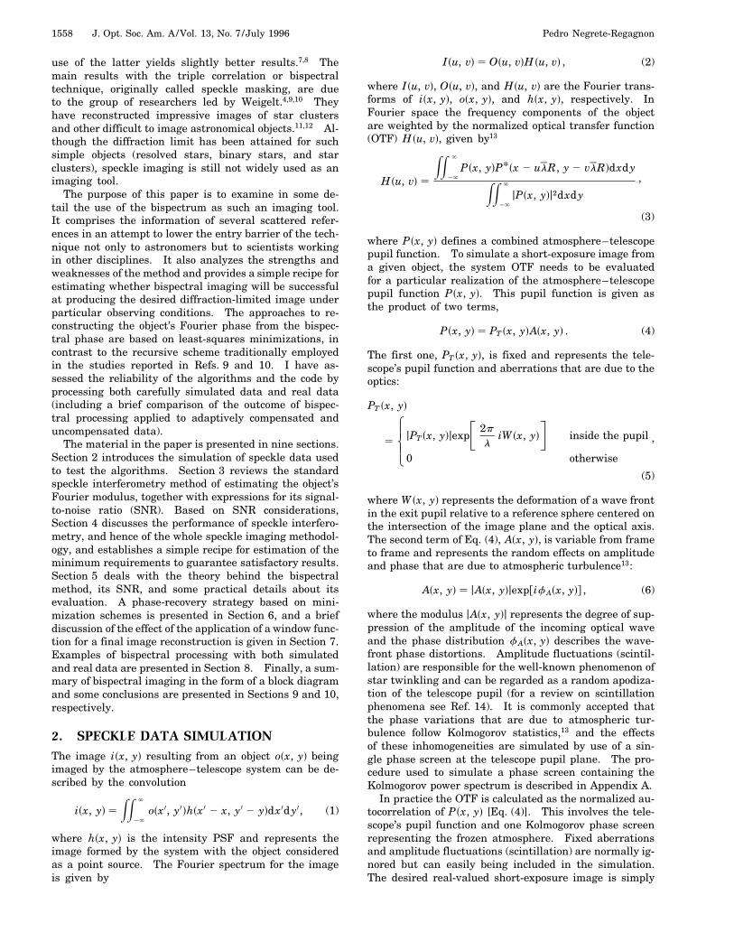


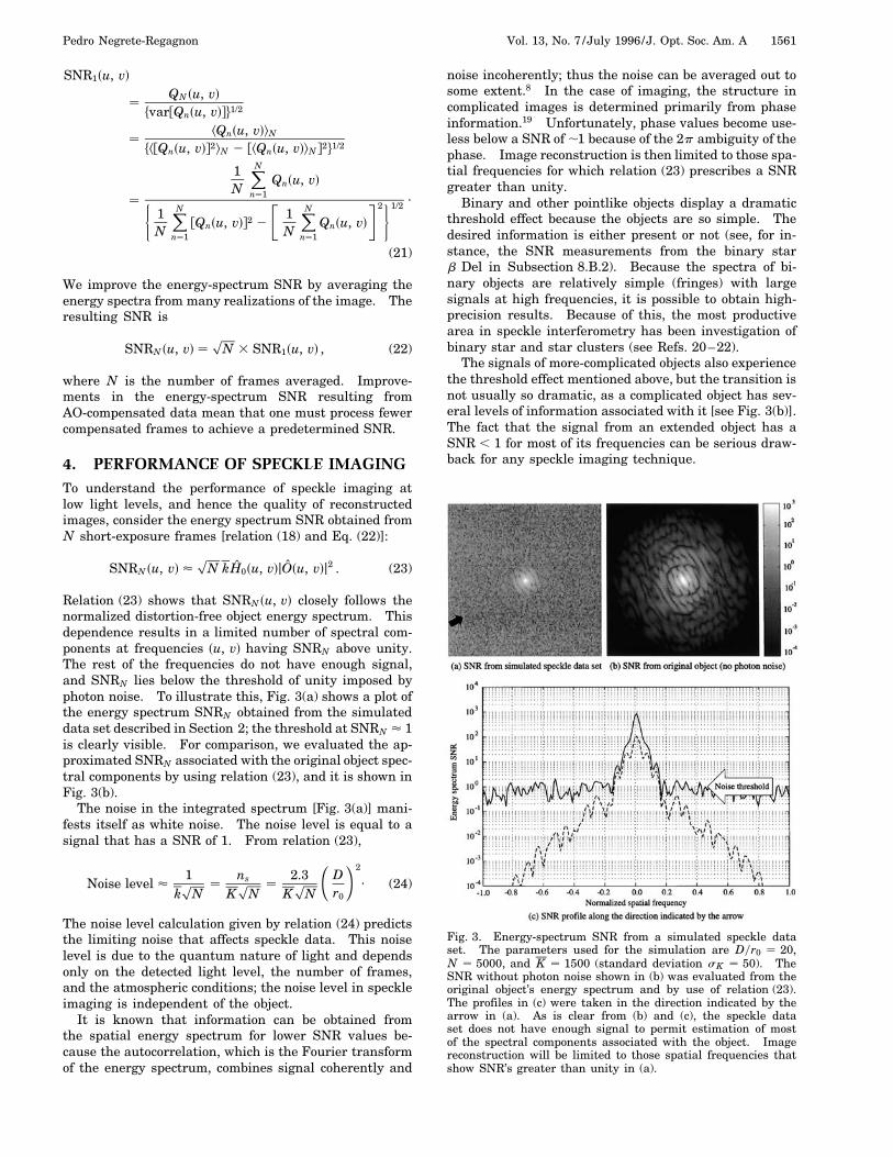


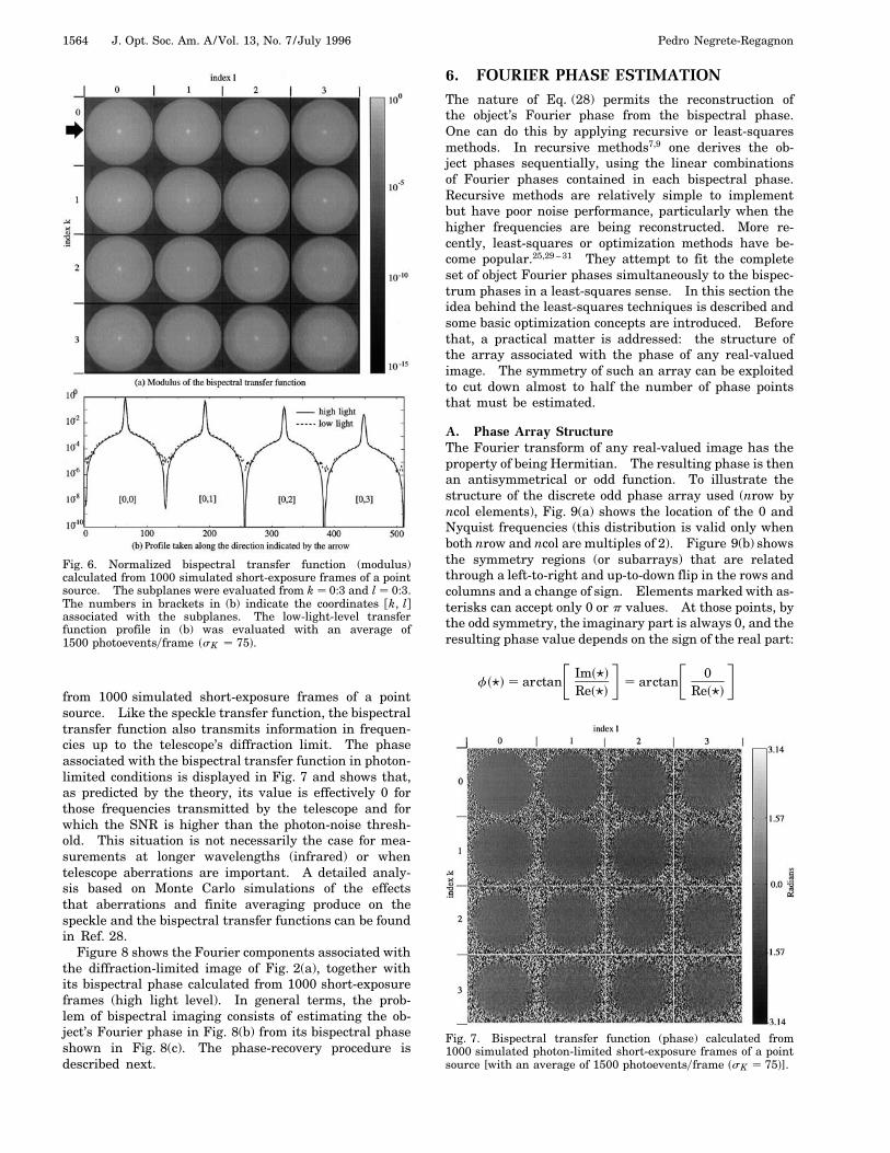


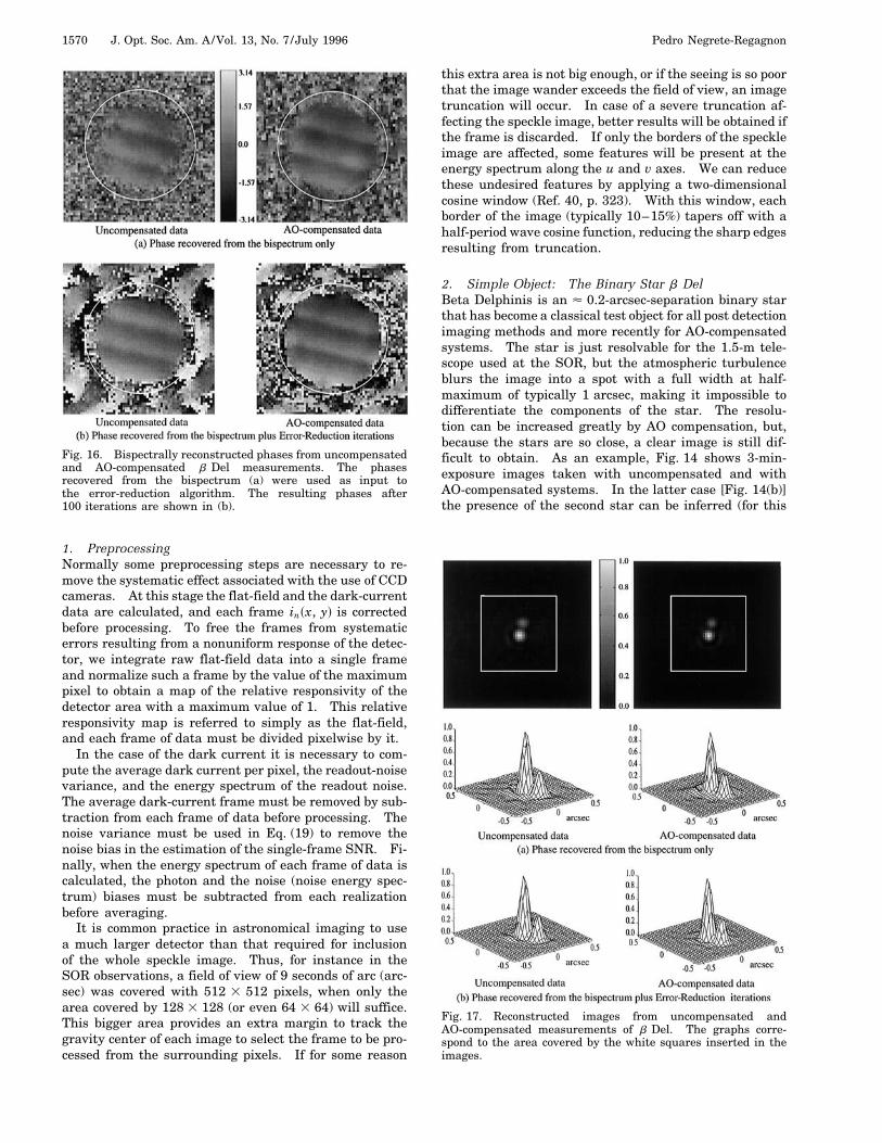

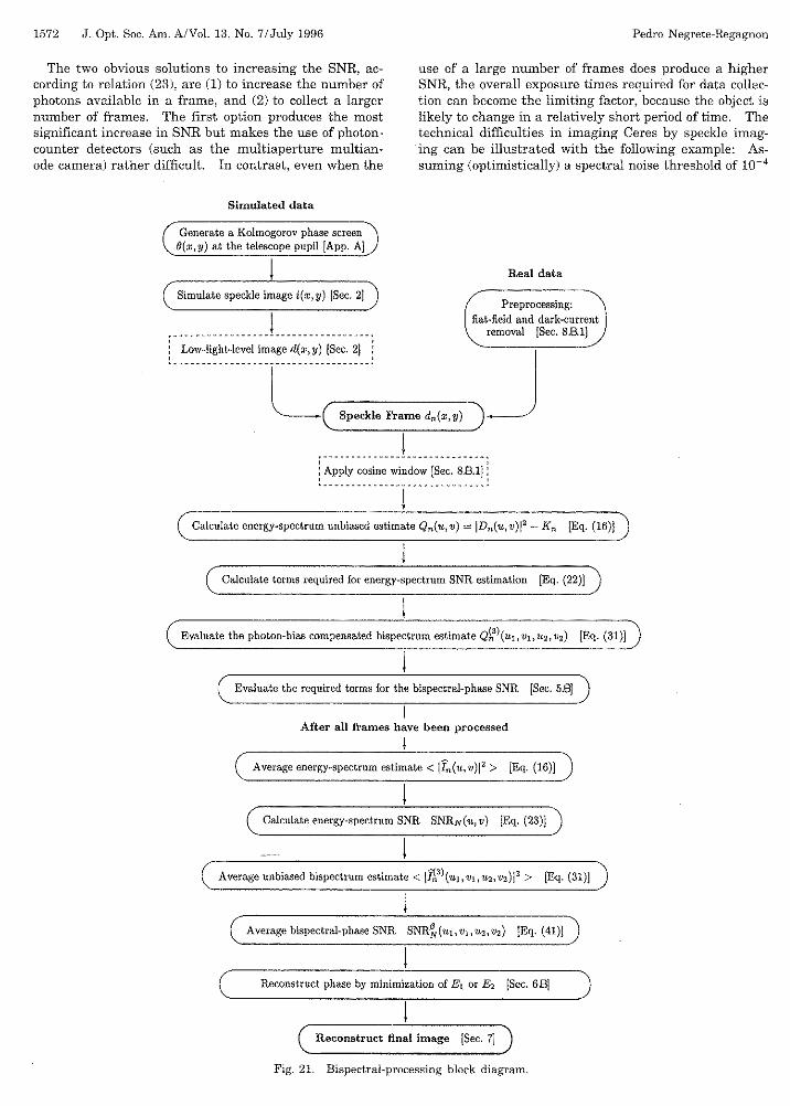


![[Recovery] Cwm Recovery 6.0.3](https://static.documents.pub/doc/80x56/55cf9443550346f57ba0c2b8/recovery-cwm-recovery-603.jpg)


