40
Practical challenges faced when using modern approaches to numerical PDEs to simulate petroleum reservoirs Halvor Møll Nilsen, SINTEF ICT
| Date post: | 21-Dec-2015 |
| Category: |
Documents |
| Upload: | osborne-lewis |
| View: | 224 times |
| Download: | 0 times |
Practical challenges faced when using modern approaches to numerical PDEs to simulate
petroleum reservoirs
Halvor Møll Nilsen, SINTEF ICT
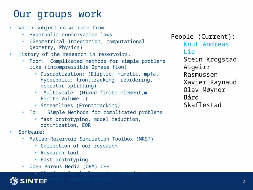
• Which subject do we come from• Hyperbolic conservation laws• (Geometrical Integration, computational geometry,
Physics)• History of the research in reservoirs,
• From: Complicated methods for simple problems like (incompressible 2phase flow)
• Discretization: (Eliptic; mimetic, mpfa, Hyperbolic: fronttracking, reordering, operator splitting)
• Multiscale (Mixed finite element,m Finite Volume .)
• Streamlines (Fronttracking) • To: Simple Methods for complicated problems
• fast prototyping, model reduction, optimization, EOR
• Software:• Matlab Reservoir Simulation Toolbox (MRST)
• Collection of our research• Research tool• Fast prototyping
• Open Porous Media (OPM) C++• Platform for implementing methods on Industry
standard models
Our groups work
2
People (Current):Knut Andreas LieStein KrogstadAtgeirr RasmussenXavier RaynaudOlav MøynerBård Skaflestad
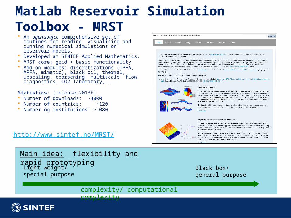
Matlab Reservoir Simulation Toolbox - MRST An open source comprehensive set of routines
for reading, visualising and running numerical simulations on reservoir models.
Developed at SINTEF Applied Mathematics. MRST core: grid + basic functionality Add-on modules: discretizations (TPFA, MPFA,
mimetic), black oil, thermal, upscaling, coarsening, multiscale, flow diagnostics, CO2 laboratory,….
Statistics: (release 2013b) Number of downloads: ~3000 Number of countries: ~120 Number og institutions: ~1080
http://www.sintef.no/MRST/
Light weight/special purpose
Black box/general purpose
complexity/ computational complexity
Main idea: flexibility and rapid prototyping

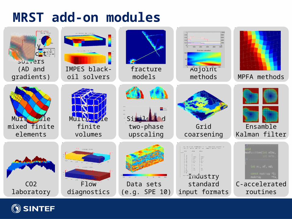
MRST add-on modules
Fully implicit solvers(AD and
gradients)IMPES black-oil
solversDiscrete
fracture models Adjoint
methods MPFA methods
Multiscale mixed finite
elementsMultiscale finite
volumes
Single and two-phase
upscaling Grid coarseningEnsamble
Kalman filter
CO2 laboratoryFlow
diagnosticsData sets
(e.g. SPE 10)
Industry standard input
formatsC-accelerated
routines
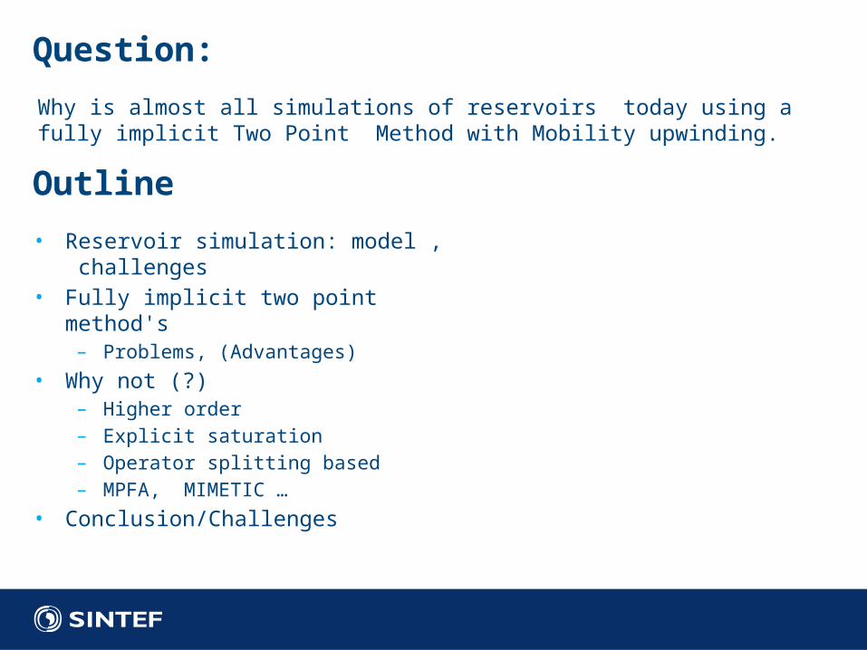
Outline
• Reservoir simulation: model , challenges
• Fully implicit two point method's– Problems, (Advantages)
• Why not (?)– Higher order– Explicit saturation– Operator splitting based– MPFA, MIMETIC …
• Conclusion/Challenges
Question:
Why is almost all simulations of reservoirs today using a fully implicit Two Point Method with Mobility upwinding.
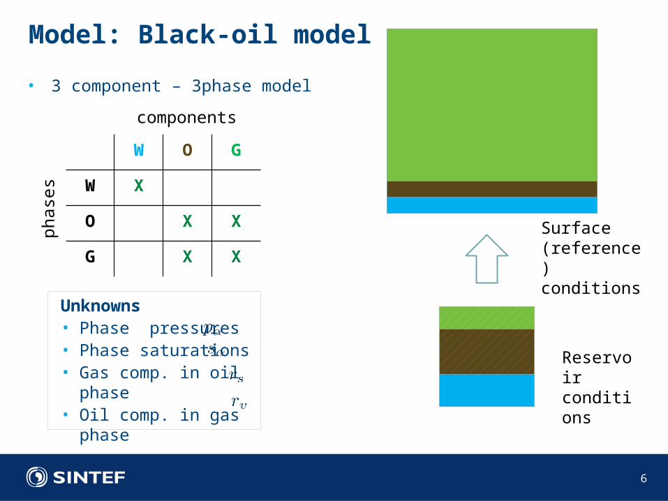
• 3 component – 3phase model
Model: Black-oil model
6
W O G
W X
O X X
G X X
phase
s
components
Reservoir conditions
Surface (reference) conditions
Unknowns• Phase pressures • Phase saturations• Gas comp. in oil
phase• Oil comp. in gas
phase
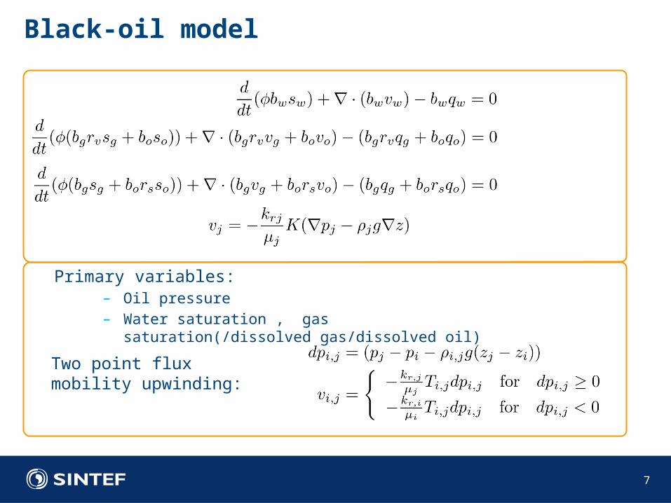
Black-oil model
7
Primary variables: – Oil pressure– Water saturation , gas saturation(/dissolved
gas/dissolved oil)
Two point flux mobility upwinding:
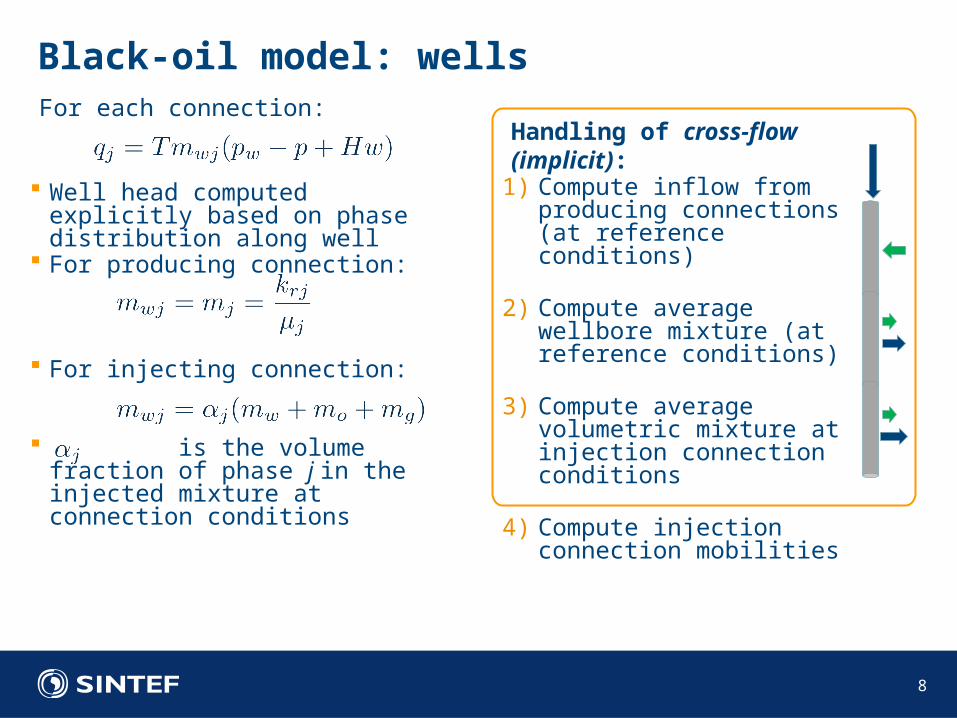
Black-oil model: wells
8
For each connection:
Well head computed explicitly based on phase distribution along well
For producing connection:
For injecting connection:
is the volume fraction of phase j in the injected mixture at connection conditions
Handling of cross-flow (implicit):
1) Compute inflow from producing connections (at reference conditions)
2) Compute average wellbore mixture (at reference conditions)
3) Compute average volumetric mixture at injection connection conditions
4) Compute injection connection mobilities
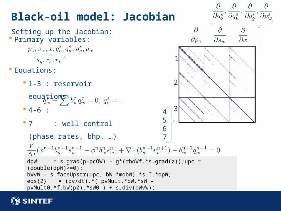
Black-oil model: JacobianSetting up the Jacobian:
Primary variables:
Equations:
1-3 : reservoir equations
4-6 :
7 : well control (phase
rates, bhp, …)
1
2
34567
dpW = s.grad(p-pcOW) - g*(rhoWf.*s.grad(z));upc = (double(dpW)>=0);bWvW = s.faceUpstr(upc, bW.*mobW).*s.T.*dpW;eqs{2} = (pv/dt).*( pvMult.*bW.*sW - pvMult0.*f.bW(p0).*sW0 ) + s.div(bWvW);
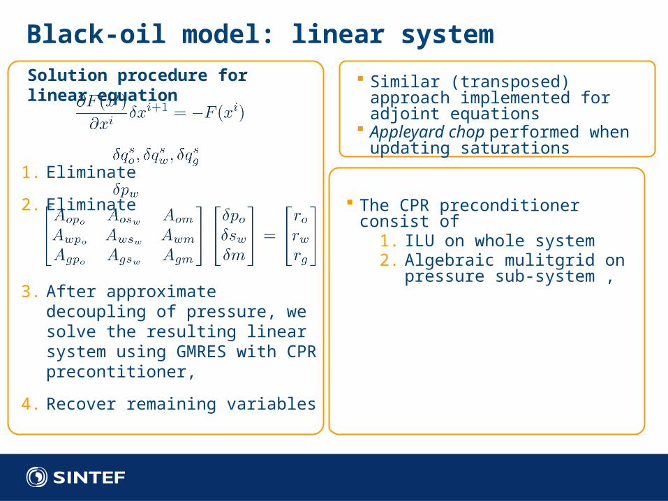
Black-oil model: linear system
Solution procedure for linear equation
1. Eliminate
2. Eliminate
3. After approximate decoupling of pressure, we solve the resulting linear system using GMRES with CPR precontitioner,
4. Recover remaining variables
Similar (transposed) approach implemented for adjoint equations
Appleyard chop performed when updating saturations
The CPR preconditioner consist of
1. ILU on whole system2. Algebraic mulitgrid on
pressure sub-system ,
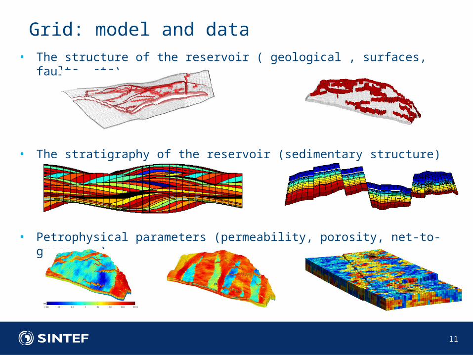
• The structure of the reservoir ( geological , surfaces, faults, etc)
• The stratigraphy of the reservoir (sedimentary structure)
• Petrophysical parameters (permeability, porosity, net-to-gross, ….)
Grid: model and data
11
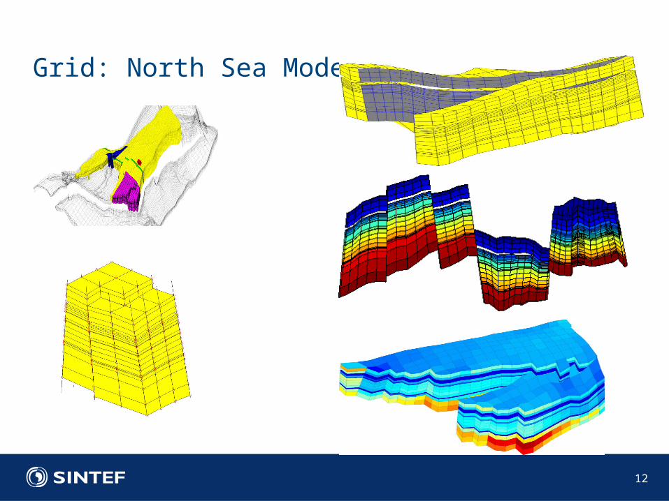
Grid: North Sea Model
12
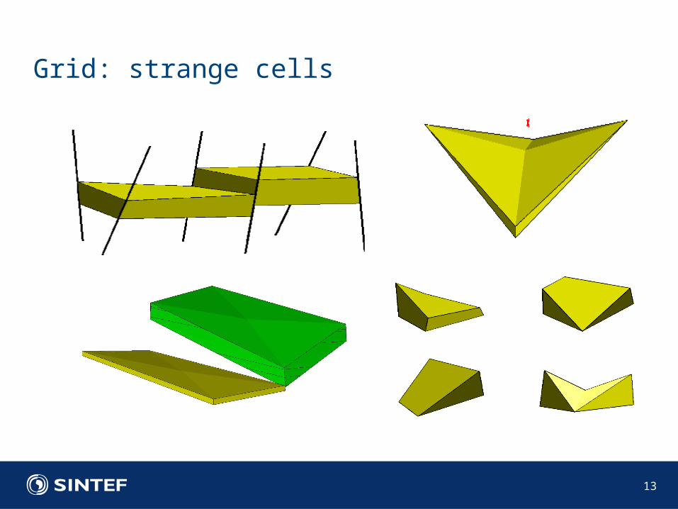
Grid: strange cells
13
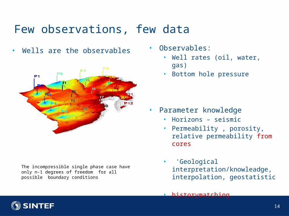
• Wells are the observables
Few observations, few data
14
• Observables:• Well rates (oil, water, gas)• Bottom hole pressure
• Parameter knowledge• Horizons – seismic• Permeability , porosity, relative
permeability from cores
• 'Geological interpretation/knowleadge, interpolation, geostatistic
• historymatching
The incompressible single phase case have only n-1 degrees of freedom for all possible boundary conditions
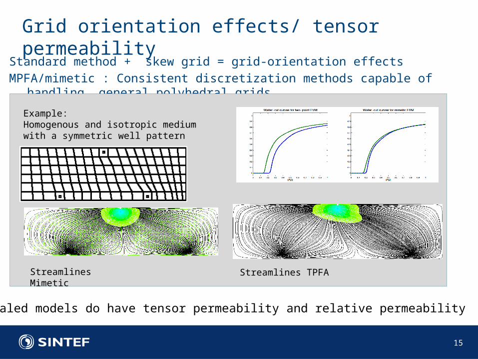
Standard method + skew grid = grid-orientation effectsMPFA/mimetic : Consistent discretization methods capable of handling
general polyhedral grids
Grid orientation effects/ tensor permeability
15
Example:Homogenous and isotropic medium with a symmetric well pattern
Water cut TPFA Water cut, mimetic
Streamlines TPFAStreamlines Mimetic
Upscaled models do have tensor permeability and relative permeability
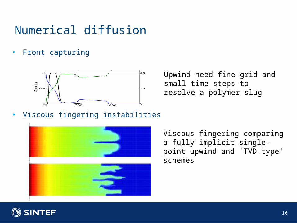
• Front capturing
• Viscous fingering instabilities
Numerical diffusion
16
Viscous fingering comparing a fully implicit single-point upwind and 'TVD-type' schemes
Upwind need fine grid and small time steps to resolve a polymer slug
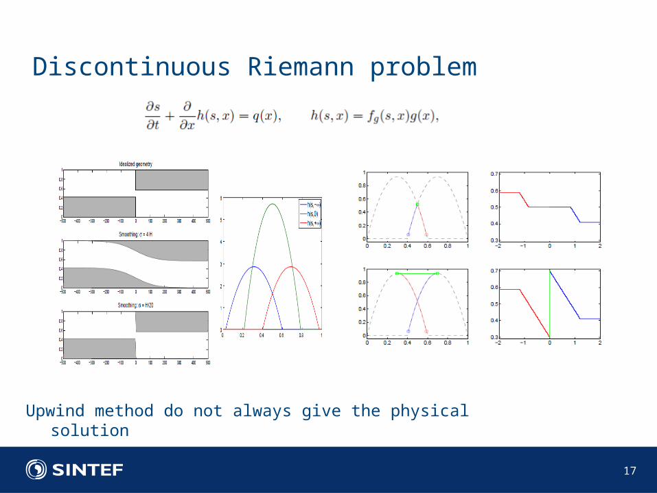
Upwind method do not always give the physical solution
Discontinuous Riemann problem
17
• Explicit• Splitting:
• Full system• Pressure and transport
• Transport:• Advection, (convection) diffusion
• High order:• MPFA, MIMETIC, Mixed finite element, DG• Parallelization:
Proposed methods:
18
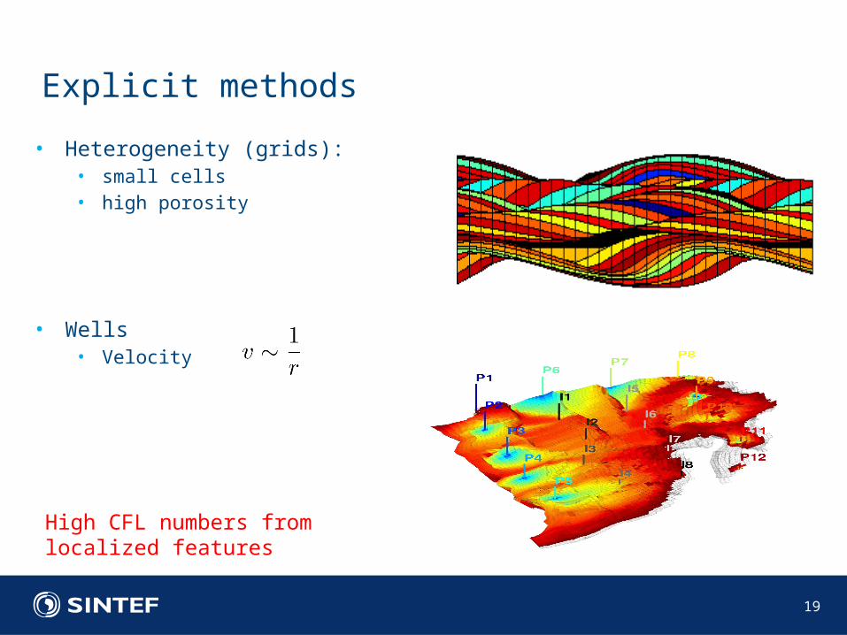
• Heterogeneity (grids):• small cells• high porosity
• Wells• Velocity
Explicit methods
19
High CFL numbers from localized features
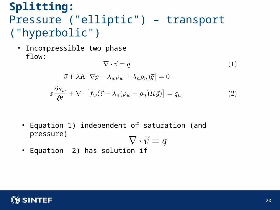
Splitting:Pressure ("elliptic") – transport ("hyperbolic")
20
• Equation 1) independent of saturation (and pressure)
• Equation 2) has solution if
• Incompressible two phase flow:
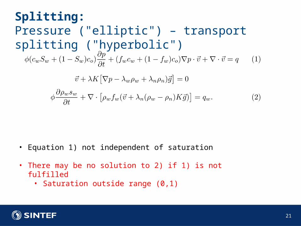
Splitting:Pressure ("elliptic") – transport splitting ("hyperbolic")
21
• Equation 1) not independent of saturation
• There may be no solution to 2) if 1) is not fulfilled• Saturation outside range (0,1)
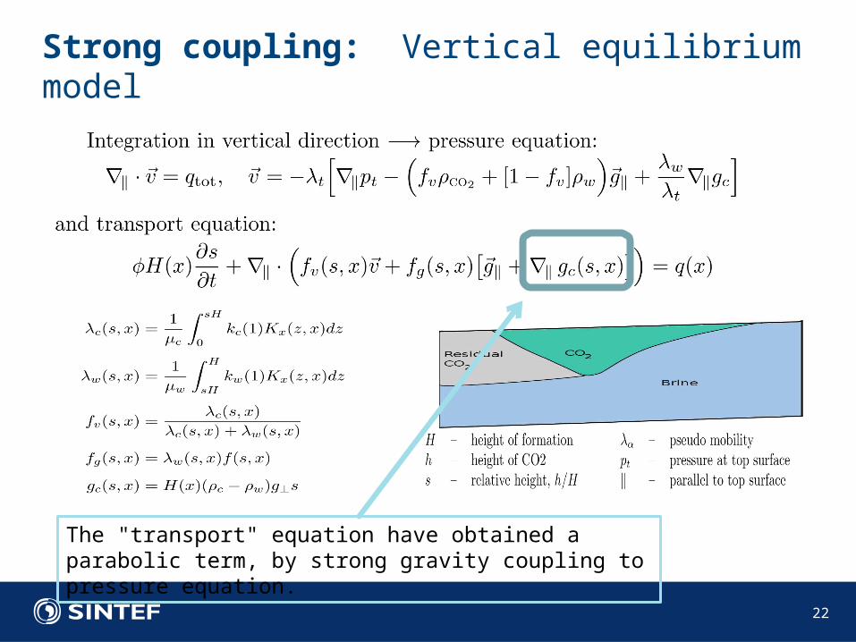
Strong coupling: Vertical equilibrium model
22
The "transport" equation have obtained a parabolic term, by strong gravity coupling to pressure equation.
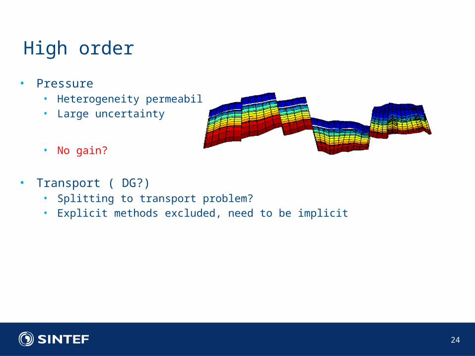
• Pressure• Heterogeneity permeability• Large uncertainty
• No gain?
• Transport ( DG?)• Splitting to transport problem?• Explicit methods excluded, need to be implicit
High order
24
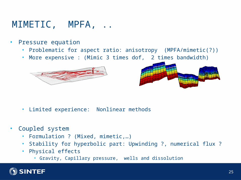
• Pressure equation• Problematic for aspect ratio: anisotropy (MPFA/mimetic(?))• More expensive : (Mimic 3 times dof, 2 times bandwidth)
• Limited experience: Nonlinear methods
• Coupled system• Formulation ? (Mixed, mimetic,…)• Stability for hyperbolic part: Upwinding ?, numerical flux ?• Physical effects
• Gravity, Capillary pressure, wells and dissolution
MIMETIC, MPFA, ..
25
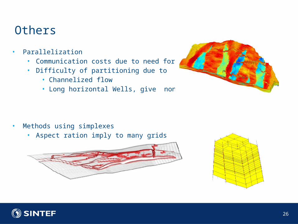
• Parallelization• Communication costs due to need for implicit solver• Difficulty of partitioning due to
• Channelized flow• Long horizontal Wells, give nonlocal connections
• Methods using simplexes• Aspect ration imply to many grids
Others
26
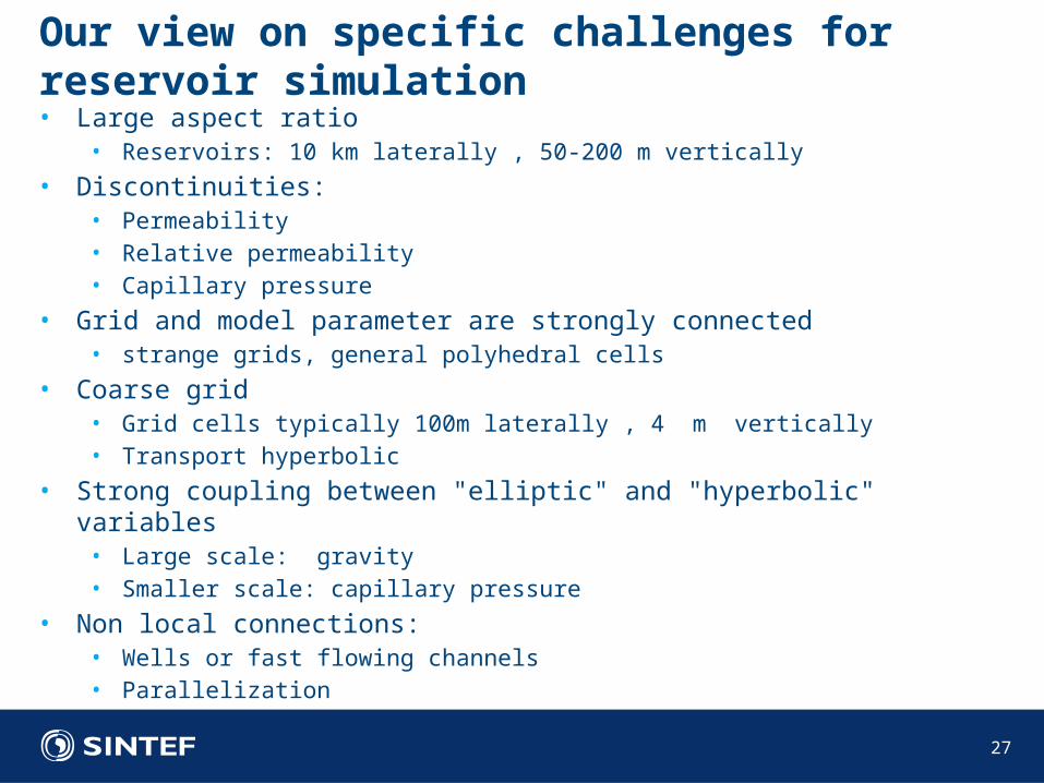
• Large aspect ratio • Reservoirs: 10 km laterally , 50-200 m vertically
• Discontinuities: • Permeability • Relative permeability • Capillary pressure
• Grid and model parameter are strongly connected• strange grids, general polyhedral cells
• Coarse grid• Grid cells typically 100m laterally , 4 m vertically• Transport hyperbolic
• Strong coupling between "elliptic" and "hyperbolic" variables• Large scale: gravity• Smaller scale: capillary pressure
• Non local connections:• Wells or fast flowing channels• Parallelization
Our view on specific challenges for reservoir simulation
27
• Research should focus on:• Methods for general challenging grid with generic implementation • Methods which work for elliptic, parabolic and hyperbolic problems• Methods for strongly coupled problems• Tensor Mobilities
• Specific purpose simulators• Codes using modern methods for correctly simplified systems
• Accept for simplifications• In reservoir simulation an fully implicit solve using TPFA and mobility upwinding is
ofhen assumed to be the truth.• Work flows including:
• Simple models• Numerical (specific) upscaled/reduced models• Trusted simulations/"Full physics simulations."
• Open source• Simulators to challenge industry simulators• Implementations of current research
• Open Data • Real reservoir models as benchmark
Conclusion: What is needed
29

30
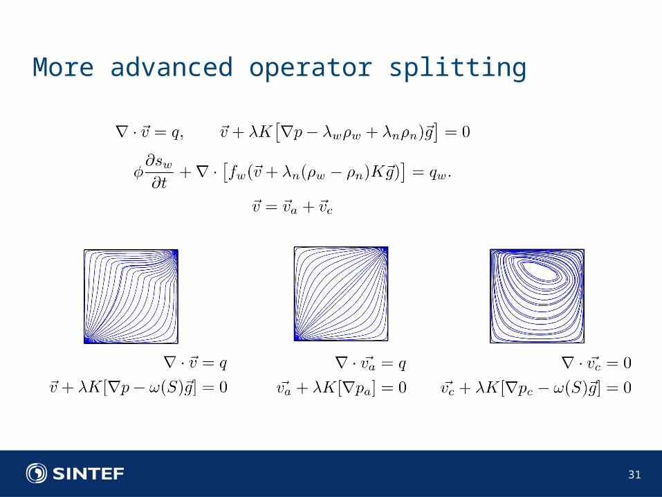
More advanced operator splitting
31
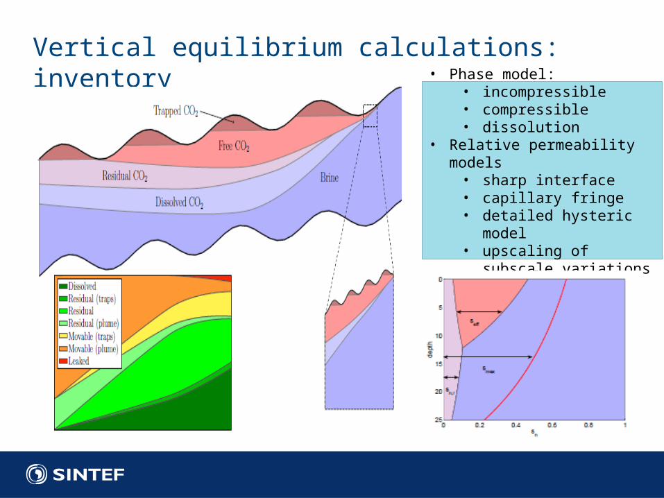
Vertical equilibrium calculations: inventory• Phase model:• incompressible• compressible• dissolution
• Relative permeability models
• sharp interface• capillary fringe• detailed hysteric
model• upscaling of subscale
variations
33
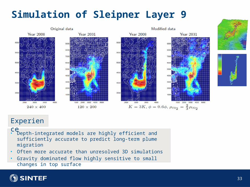
• Depth-integrated models are highly efficient and sufficiently accurate to predict long-term plume migration
• Often more accurate than unresolved 3D simulations• Gravity dominated flow highly sensitive to small changes in
top surface
Simulation of Sleipner Layer 9
Experience
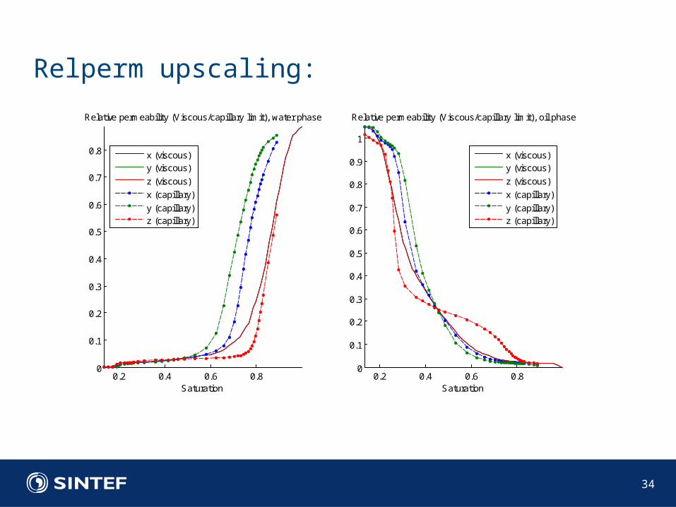
Relperm upscaling:
34
0.2 0.4 0.6 0.80
0.1
0.2
0.3
0.4
0.5
0.6
0.7
0.8
Relative permeability (Viscous/capillary limit), water phase
Saturation
x (viscous)y (viscous)
z (viscous)
x (capillary)
y (capillary)z (capillary)
0.2 0.4 0.6 0.80
0.1
0.2
0.3
0.4
0.5
0.6
0.7
0.8
0.9
1
Relative permeability (Viscous/capillary limit), oil phase
Saturation
x (viscous)y (viscous)
z (viscous)
x (capillary)
y (capillary)z (capillary)
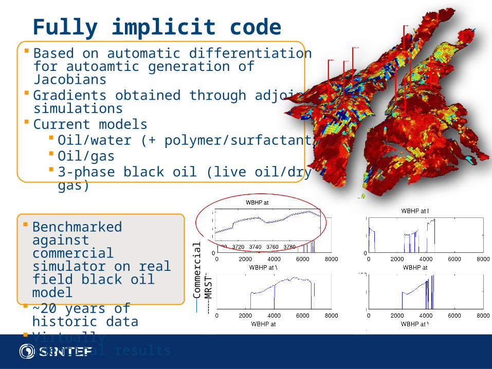
Fully implicit code Based on automatic differentiation for
autoamtic generation of Jacobians Gradients obtained through adjoint
simulations Current models
Oil/water (+ polymer/surfactant) Oil/gas 3-phase black oil (live oil/dry gas)
Benchmarked against commercial simulator on real field black oil model
~20 years of historic data
Virtually identical results
Com
mer
cial
MR
ST
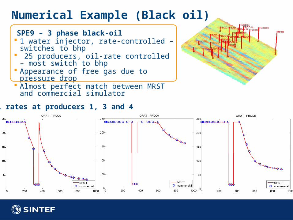
Numerical Example (Black oil)
SPE9 – 3 phase black-oil 1 water injector, rate-controlled –
switches to bhp 25 producers, oil-rate controlled – most
switch to bhp Appearance of free gas due to pressure
drop Almost perfect match between MRST and
commercial simulator
Oil rates at producers 1, 3 and 4
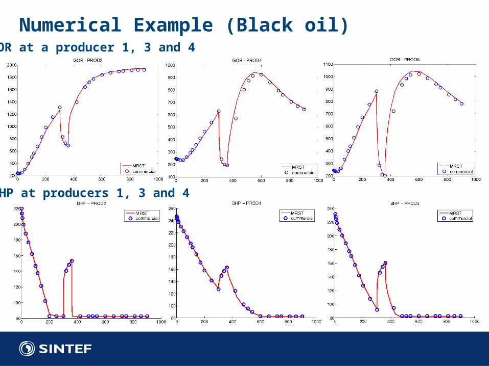
GOR at a producer 1, 3 and 4
BHP at producers 1, 3 and 4
Numerical Example (Black oil)
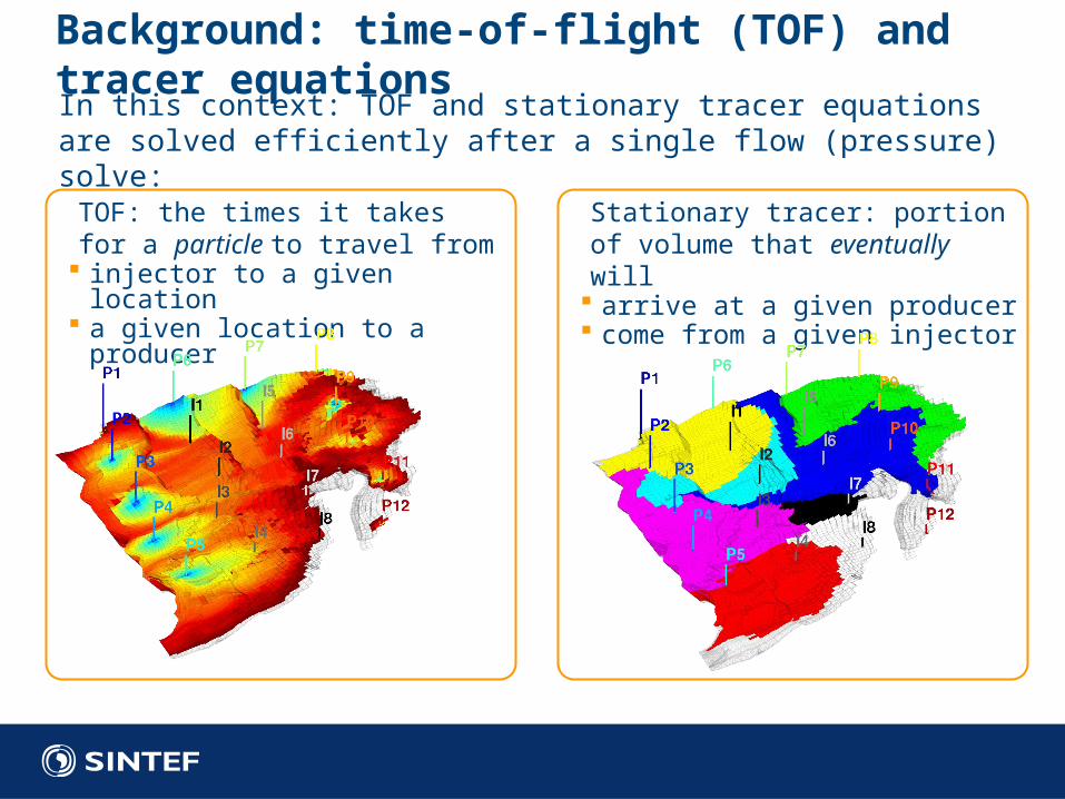
Background: time-of-flight (TOF) and tracer equationsIn this context: TOF and stationary tracer equations are solved efficiently after a single flow (pressure) solve:
TOF: the times it takes for a particle to travel from
injector to a given location a given location to a producer
Stationary tracer: portion of volume that eventually will
arrive at a given producer come from a given injector

Diagnostics based on time-of-flight (TOF) and tracersEfficient ranking of geomodels Reduce ensamble prior to (upscaling and) full
simulation Need measures that correlate well with e.g.,
receovery prediction
Validation of upscaling Use allocation factors for assessing quality of
upscaling
Visualization See flow-paths, regions of influence, interaction
regions etc Immediately see effect of new well-placements, model
updates etc.
Optimization Use as proxies in optimization to find good initial
guesses. Need measures that correlate well to objective (e.g,
NPV)
MRST add-on modules
Fully implicit solvers(AD and
gradients)IMPES black-oil
solversDiscrete
fracture models Adjoint
methods MPFA methods
Multiscale mixed finite
elementsMultiscale finite
volumes
Single and two-phase
upscaling Grid coarseningEnsamble
Kalman filter
CO2 laboratoryFlow
diagnosticsData sets
(e.g. SPE 10)
Industry standard input
formatsC-accelerated
routines
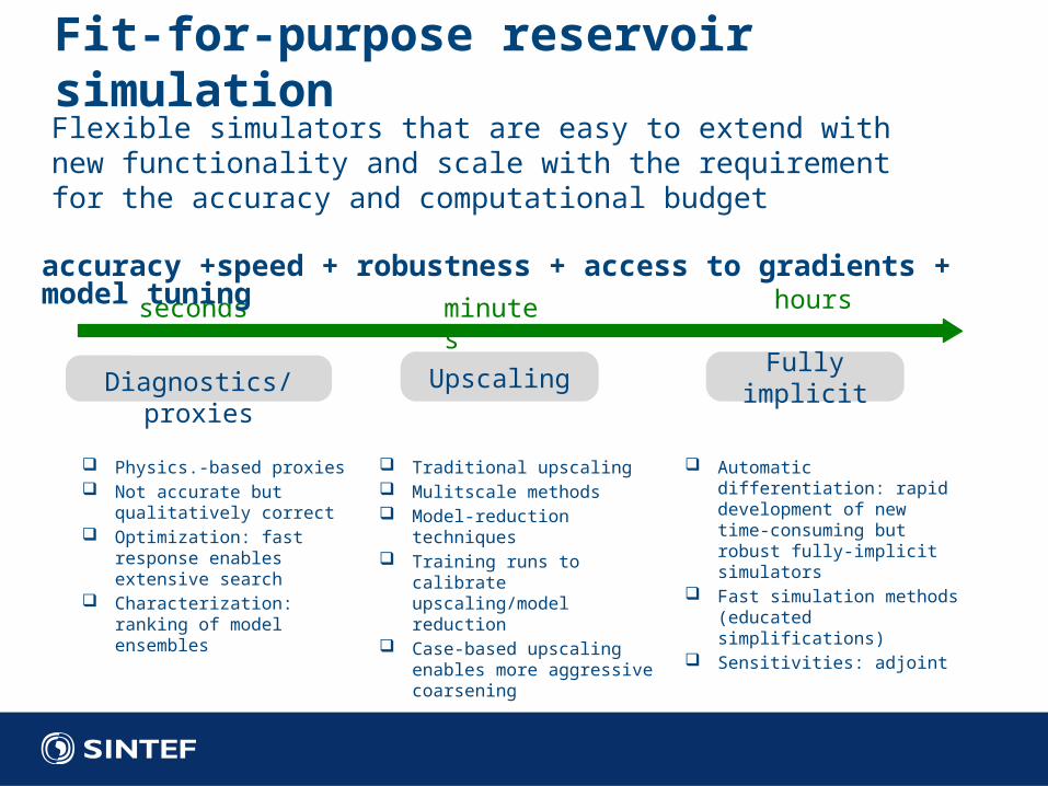
Fit-for-purpose reservoir simulation
seconds
Diagnostics/proxies Upscaling Fully implicit
minutes hours
Flexible simulators that are easy to extend with new functionality and scale with the requirement for the accuracy and computational budget
accuracy +speed + robustness + access to gradients + model tuning
Physics.-based proxies Not accurate but
qualitatively correct Optimization: fast
response enables extensive search
Characterization: ranking of model ensembles
Traditional upscaling Mulitscale methods Model-reduction techniques Training runs to calibrate
upscaling/model reduction Case-based upscaling
enables more aggressive coarsening
Automatic differentiation: rapid development of new time-consuming but robust fully-implicit simulators
Fast simulation methods (educated simplifications)
Sensitivities: adjoint
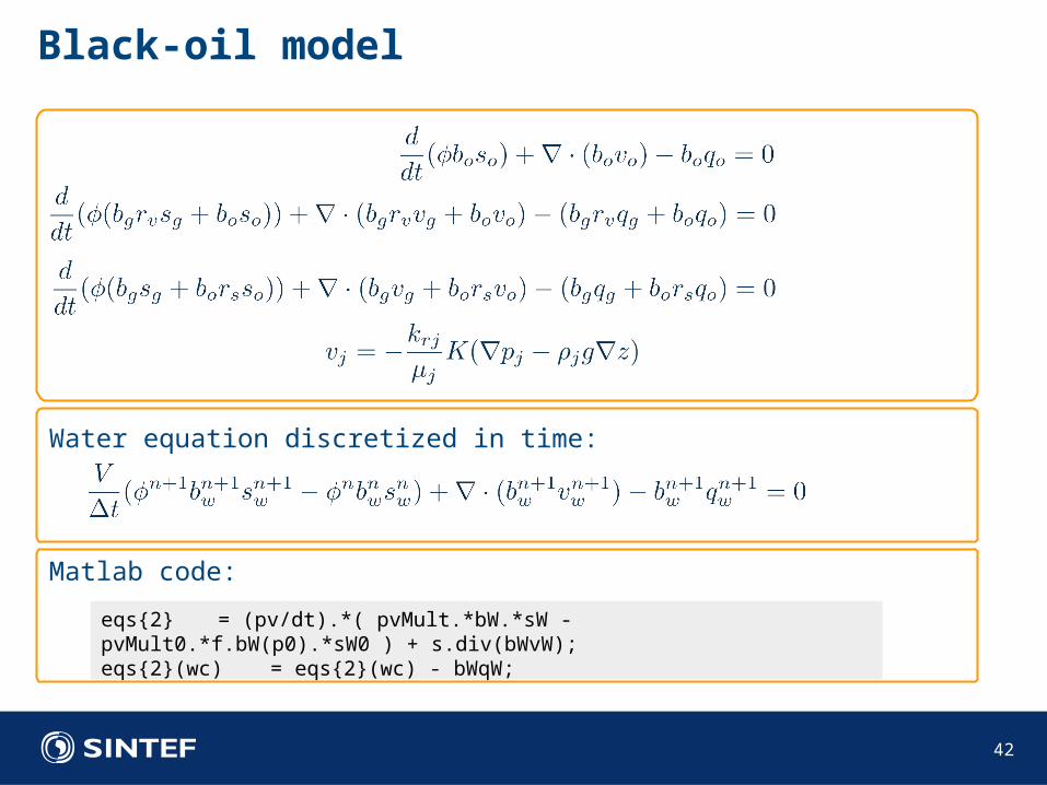
Black-oil model
42
Water equation discretized in time:
eqs{2} = (pv/dt).*( pvMult.*bW.*sW - pvMult0.*f.bW(p0).*sW0 ) + s.div(bWvW);eqs{2}(wc) = eqs{2}(wc) - bWqW;
Matlab code:


