Page 1
Pre-treatment processing of household
plastic packaging waste
Ross Blackstock (Student number: 767366)
School of Mechanical, Industrial and Aeronautical Engineering
University of the Witwatersrand
Johannesburg, South Africa.
Supervisors: Bernadette Sunjka (School of Mechanical, Industrial and Aeronautical Engineering)
and Lizelle Van Dyk (School of Chemical and Metallurgical Engineering)
A research report submitted to the Faculty of Engineering and the Built Environment, University of
the Witwatersrand, in fulfilment of the requirements for the degree of Masters in Engineering.
Johannesburg, 2016
Page 2
i
Declaration
I declare that this research report is my own unaided work. It is being submitted to the Degree of
Master of Science in Engineering to the University of the Witwatersrand, Johannesburg. It has not been
submitted before for any degree or examination to any other university.
11th day of September 2016
Page 3
i
Abstract
The purpose of this investigation was to investigate whether or not it would be possible to separate
blow moulded and injection moulded waste plastics using two techniques; air classification and
ballistic separation. Air classification and ballistic separation are two techniques that separate different
types of material according to size, shape and density. Previous research, together with new
measurements, has suggested that blow mould plastics tend to be thinner in terms of wall thickness
than injection moulded plastics meaning that air classification could be used to separate each type of
plastic. The material used for the study was supplied by a Romanian recycler and was a mixture of High
Density Polyethylene and polypropylene. Two additional samples, one Polyethylene rich and the other
polypropylene rich, were also included in the research.
The first part of the study involved measuring different characteristics of the material to determine
how to go about performing the different air classification experiments. The second part of the study
focused on separating the different material samples using different air classifier systems and a ballistic
separation system. The third part of the study focused on processing the samples from part 2 (air
classification) into test specimens for further mechanical and melt flow property measurements.
After measuring the mechanical and melt flow properties of the different samples it was found that air
classification did not substantially improve the mechanical or melt flow properties of the material. The
study did, however, show that there is a strong correlation between polymer type and melt flow
properties. High Density polypropylene is generally used for blow mould applications whereas
polypropylene is generally used for injection mould applications. Separating the material according to
polymer type therefore means that the material is, to an extent, also sorted according to melt flow
properties.
Page 4
ii
Acknowledgements
I would like to thank my supervisors Dr Lizelle Van Dyk, Dr Norbert Fraunholcz and Ms Bernadette
Sunjka for their support and guidance. I would also like to thank Prof. Peter Rem at Delft University of
Technology for giving me access to the laboratory facilities at the university, and for his invaluable
advice. Finally, I would like to thank Mr. Jaap Vandehoek for the internship position that allowed me
to complete this research in the Netherlands.
Page 5
iii
Contents
Declaration ............................................................................................................................................... i
Nomenclature ........................................................................................................................................... x
List of acronyms.........................................................................................................................................
CHAPTER 1 ................................................................................................................................... 1
1 Introduction ..................................................................................................................................... 1
1.1 Project background ................................................................................................................. 3
1.1.1 Magnetic Density Separation .......................................................................................... 3
1.1.2 Melt Flow Index ............................................................................................................... 4
1.1.3 Recycling facility .............................................................................................................. 4
1.2 Objectives of the study ............................................................................................................ 5
1.3 Scope of the study ................................................................................................................... 7
1.4 Limitations and constraints ..................................................................................................... 7
1.5 Structure of the report ............................................................................................................ 7
CHAPTER 2 ................................................................................................................................... 9
2 Literature review ............................................................................................................................. 9
2.1 European polymer industry ..................................................................................................... 9
2.1.1 Plastic packaging.............................................................................................................. 9
2.1.2 Waste management ...................................................................................................... 10
2.1.3 Plastic recycling ............................................................................................................. 12
2.2 Magnetic Density Separation ................................................................................................ 13
2.3 Polymers ................................................................................................................................ 14
2.3.1 Types of polymers ......................................................................................................... 14
2.3.2 Properties of thermoplastics ......................................................................................... 15
2.3.3 Virgin polymer production ............................................................................................ 18
2.3.4 Polymer additives .......................................................................................................... 18
2.4 Rheology of plastics ............................................................................................................... 21
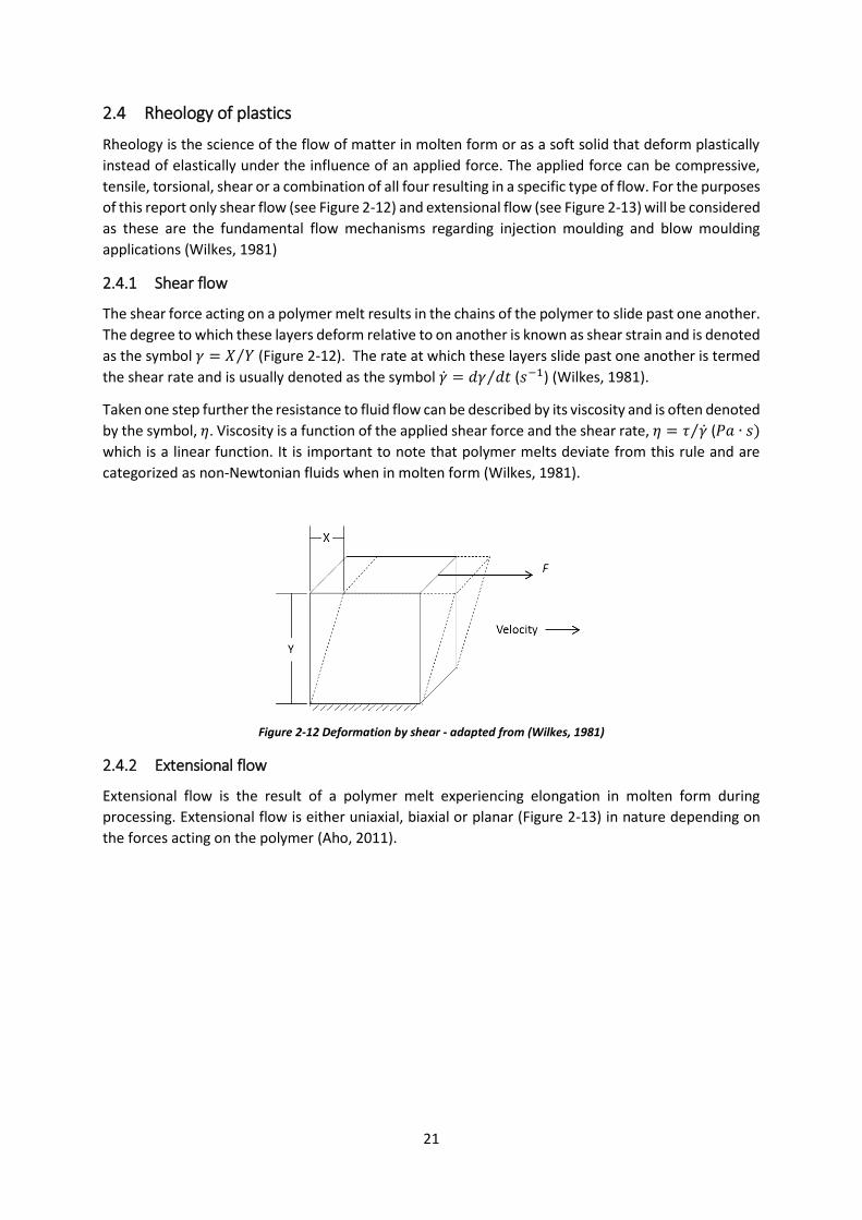
2.4.1 Shear flow ...................................................................................................................... 21
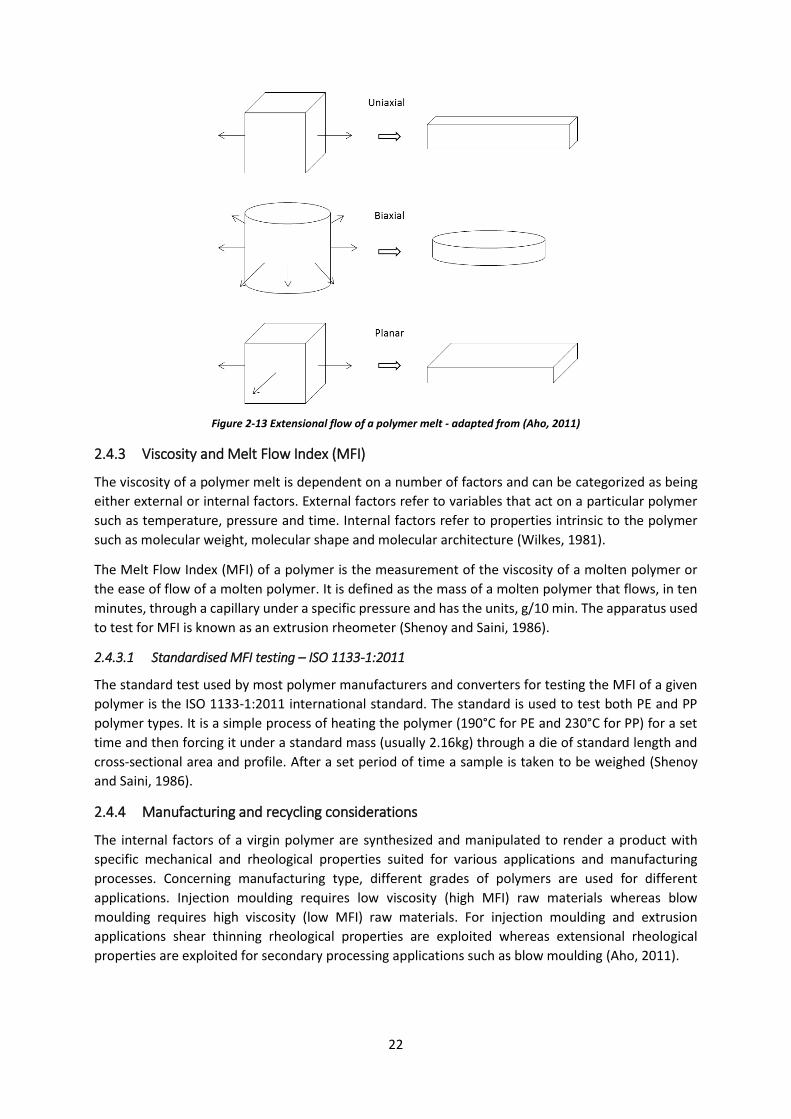
2.4.2 Extensional flow ............................................................................................................ 21
2.4.3 Viscosity and Melt Flow Index (MFI) ............................................................................. 22
2.4.4 Manufacturing and recycling considerations ................................................................ 22
2.5 Plastic packaging characterisation ........................................................................................ 23
2.5.1 Density distribution ....................................................................................................... 24
2.5.2 Rheological properties ................................................................................................... 24
Page 6
iv
2.6 Mechanical recycling ............................................................................................................. 25
2.6.1 Polymer degradation ..................................................................................................... 26
2.7 Fundamentals of particles in a fluid flow .............................................................................. 28
2.7.1 Shape considerations .................................................................................................... 28
2.7.2 Internal flow through a duct ......................................................................................... 29
2.7.3 Particles in a fluid flow .................................................................................................. 29
2.7.4 Terminal (settling) velocity of a particle in the presence of buoyancy force ................ 29
2.7.5 Ballistic trajectory .......................................................................................................... 31
2.8 Air classification ..................................................................................................................... 31
2.8.1 Introduction ................................................................................................................... 31
2.8.2 Types of separation zones ............................................................................................. 32
2.8.3 Cascade (Zigzag) air classifiers ....................................................................................... 32
2.9 Literature summary ............................................................................................................... 35
CHAPTER 3 ................................................................................................................................. 36
3 Experimental methods .................................................................................................................. 36
3.1 Overview ................................................................................................................................ 36
3.2 Experimental equipment ....................................................................................................... 36
3.3 Results ................................................................................................................................... 37
3.4 Description of the plastic samples ........................................................................................ 38
3.4.1 Pre-Magnetic Density Separation (MDS) samples ........................................................ 38
3.4.2 Test matrix ..................................................................................................................... 39
3.4.3 Post-Magnetic Density Separation (MDS) samples ....................................................... 39
3.5 Physical characterization of the material .............................................................................. 39
3.5.1 Size measurements ....................................................................................................... 40
3.5.2 Thickness measurements .............................................................................................. 41
3.5.3 Density measurements .................................................................................................. 42
3.5.4 Bulk density measurements .......................................................................................... 42
3.6 Settling velocity measurements ............................................................................................ 42
3.6.1 Material preparation ..................................................................................................... 43
3.6.2 Settling velocity determination – Drop test .................................................................. 43
3.6.3 Settling velocity determination – Flow chamber .......................................................... 43
3.7 Air classification ..................................................................................................................... 44
3.7.1 Material preparation ..................................................................................................... 45
3.7.2 Nihot® Amsterdam WS-Z zigzag air classifier ................................................................ 46
Page 7
v
3.7.3 Herbold® SZS air classifier ............................................................................................. 48
3.7.4 Herbold® feed rate assessment..................................................................................... 51
3.8 Alternative separation method - Ballistic separation............................................................ 51
3.9 Material property measurements ......................................................................................... 53
3.9.1 Test sample preparation – Injection moulding ............................................................. 54
3.9.2 Tensile properties .......................................................................................................... 55
3.9.3 Impact testing ................................................................................................................ 57
3.9.4 Melt Flow Rate test ....................................................................................................... 58
3.9.5 Differential Scanning Calorimetry test .......................................................................... 60
CHAPTER 4 ................................................................................................................................. 61
4 Results and discussion ................................................................................................................... 61
4.1 Size measurements ............................................................................................................... 61
4.2 Thickness measurements ...................................................................................................... 62
4.2.1 Mixed sample thickness distribution ............................................................................. 62
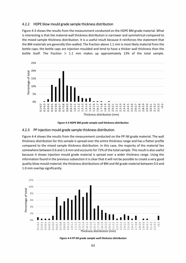
4.2.2 HDPE blow mould grade sample thickness distribution ............................................... 63
4.2.3 PP injection mould grade sample thickness distribution .............................................. 63
4.2.4 HDPE blow mould and injection mould grade sample thickness distribution .............. 64
4.2.5 Correlation between wall thickness and polymer type ................................................. 64
4.3 Density measurements .......................................................................................................... 65
4.4 Settling velocity measurements ............................................................................................ 65
4.5 Air classification ..................................................................................................................... 66
4.5.1 Nihot® air classification ................................................................................................. 66
4.5.2 Herbold® air classification ............................................................................................. 68
4.5.3 Bulk density measurements .......................................................................................... 71
4.6 Alternative separation method – Ballistic separation ........................................................... 71
4.7 Results comparison – Nihot®, Herbold®, and Ballistic separation ........................................ 72
4.8 Material property measurements ......................................................................................... 73
4.8.1 Tensile test results ......................................................................................................... 73
4.8.2 Melt Flow Rate test results ............................................................................................ 76
4.8.3 DCS test results .............................................................................................................. 77
4.9 Process configuration ............................................................................................................ 78
4.9.1 Current processing scenario .......................................................................................... 78
4.9.2 Proposed processing scenario ....................................................................................... 79
Page 8
vi
CHAPTER 5 ................................................................................................................................. 82
5 Conclusions and recommendations for future work .................................................................... 82
5.1 General conclusions .............................................................................................................. 82
5.2 Recommendations for future work ....................................................................................... 82
References ................................................................................................................................. 83
Appendix ...................................................................................................................................... i
Appendix 1 - Size distribution measurement ....................................................................................... i
Appendix 2 - Wall thickness distribution measurement ...................................................................... i
Appendix 3 - Density distribution measurement .................................................................................ii
Appendix 4 - Nihot® zigzag classifier ................................................................................................... iii
Appendix 5 - Herbold Zigzag air classifier ............................................................................................ iv
Appendix 6 - Research project consent forms .................................................................................... vi
Page 9
vii
Figures
Figure 1-1 Common packaging plastics and their associated resin codes .............................................. 1
Figure 1-2 Plastic packaging flows ........................................................................................................... 2
Figure 1-3 Plastic separation overview ................................................................................................... 3
Figure 1-4 Recycling plant process overview .......................................................................................... 4
Figure 1-5 Correlation between wall thickness and manufacturing process .......................................... 5
Figure 1-6 Pre-MDS separation ............................................................................................................... 6
Figure 1-7 Post-MDS separation .............................................................................................................. 6
Figure 1-8 System throughput and performance measurement ............................................................ 7
Figure 2-1 Plastics demand by sector in 2013 ......................................................................................... 9
Figure 2-2 Packaging plastics consumption by polymer type in Europe ............................................... 10
Figure 2-3 Packaging products .............................................................................................................. 10
Figure 2-4 Plastic waste management .................................................................................................. 11
Figure 2-5 European landfill scenarios .................................................................................................. 12
Figure 2-6 Magnetic Density Separation .............................................................................................. 13
Figure 2-7 Density gradient of magnetic fluid in the presence of a magnet ......................................... 14
Figure 2-8 Ethylene transformation to polypropylene.......................................................................... 15
Figure 2-9 Polymer structures ............................................................................................................... 16
Figure 2-10 Tacticity .............................................................................................................................. 17
Figure 2-11 Impact of stabilizers on recycled PP ................................................................................... 20
Figure 2-12 Deformation by shear ........................................................................................................ 21
Figure 2-13 Extensional flow of a polymer melt ................................................................................... 22
Figure 2-14 Density distribution of Romanian PP and PE ..................................................................... 24
Figure 2-15 Mould type – polymer type correlation ............................................................................. 25
Figure 2-16 Thickness distribution of Romanian blow mould and injection mould plastics ................. 25
Figure 2-17 Mechanical recycling scenario ........................................................................................... 26
Figure 2-18 Ellipse for representing approximate dimensions of a particle ......................................... 28
Figure 2-19 Cascade classifiers .............................................................................................................. 32
Figure 2-20 Cross section and velocity profile of a typical zigzag air classifier ..................................... 33
Figure 3-1 Overview of experimental method ...................................................................................... 36
Figure 3-2 Material sample ................................................................................................................... 39
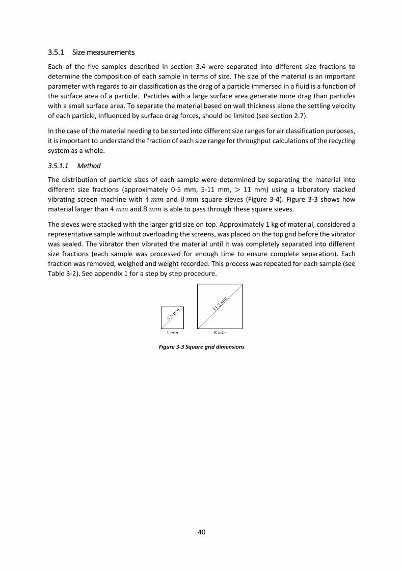
Figure 3-3 Square grid dimensions ........................................................................................................ 40
Figure 3-4 Apparatus for size measurement tests ................................................................................ 41
Figure 3-5 Settling velocity flake selection ............................................................................................ 43
Figure 3-6: Flow chamber setup ............................................................................................................ 44
Figure 3-7 Air classification before polymer type separation ............................................................... 45
Figure 3-8 MDS processing .................................................................................................................... 46
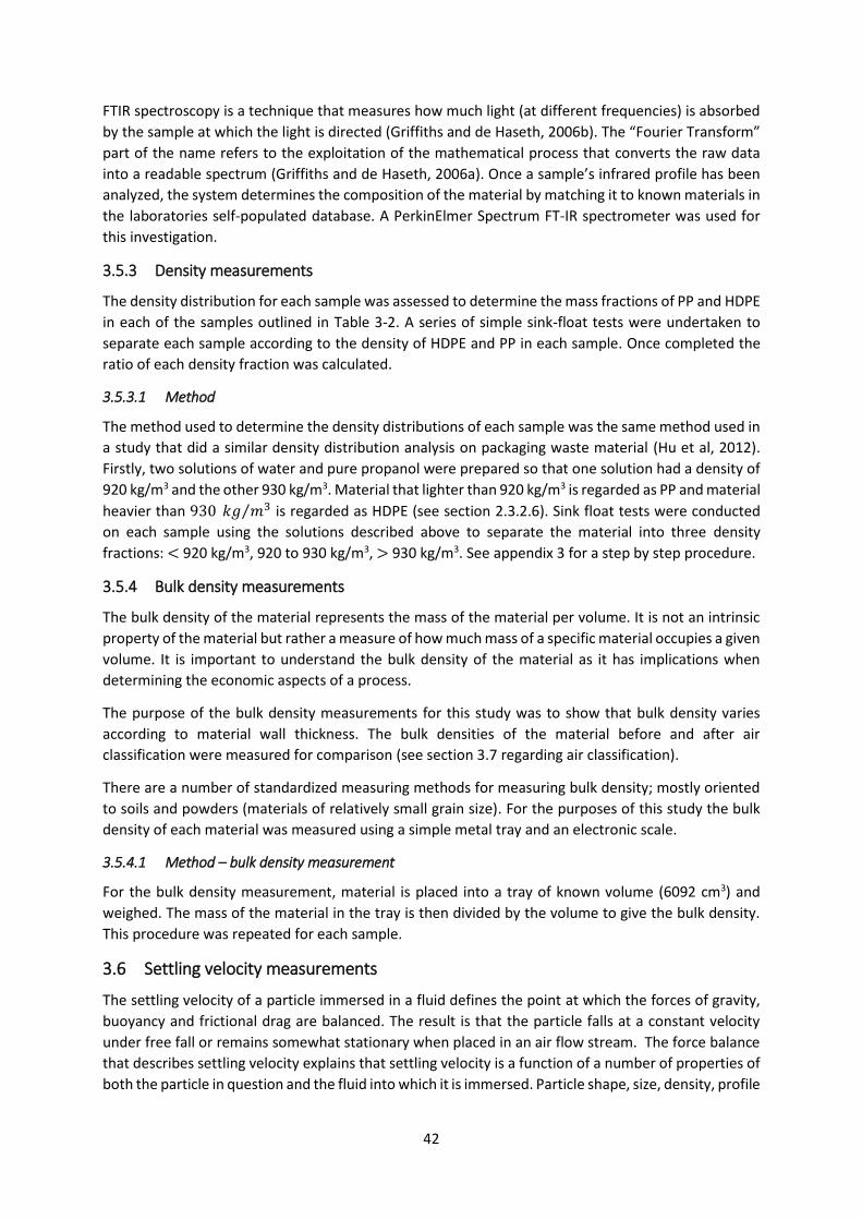
Figure 3-9 Nihot® laboratory setup ....................................................................................................... 47
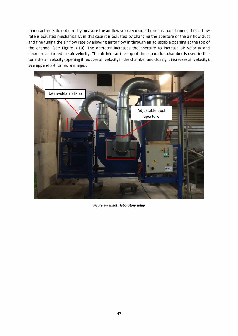
Figure 3-10 Nihot® WS-Z zigzag shifter ................................................................................................. 48
Figure 3-11 Herbold® SZS 630/212 Air classifier ................................................................................... 49
Figure 3-12 Herbold® SZS 630/212 engineering drawing ..................................................................... 50
Figure 3-13 Ballistic separator setup ..................................................................................................... 52
Figure 3-14 force diagrams .................................................................................................................... 52
Figure 3-15 Ballistic setup ..................................................................................................................... 53
Page 10
viii
Figure 3-16 Arbrurg Allrounder® 320 S 500-150 injection moulder ..................................................... 54
Figure 3-17 Typical injection moulder configuration ............................................................................ 55
Figure 3-18 Injection moulded tensile and impact specimen ............................................................... 55
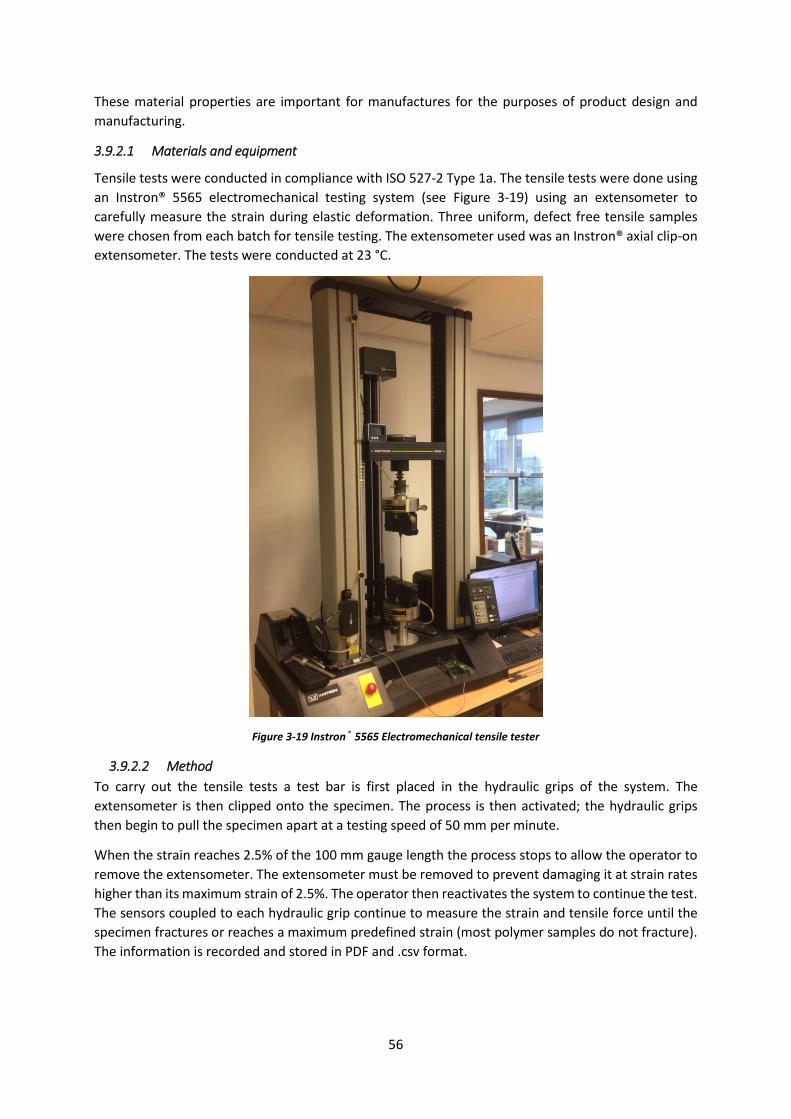
Figure 3-19 Instron® 5565 Electromechanical tensile tester ................................................................ 56
Figure 3-20 Charpy impact energy calculation ...................................................................................... 57
Figure 3-21 Charpy impact specimen .................................................................................................... 57
Figure 3-22 Impact test equipment ....................................................................................................... 58
Figure 3-23 Impact specimen in place ................................................................................................... 58
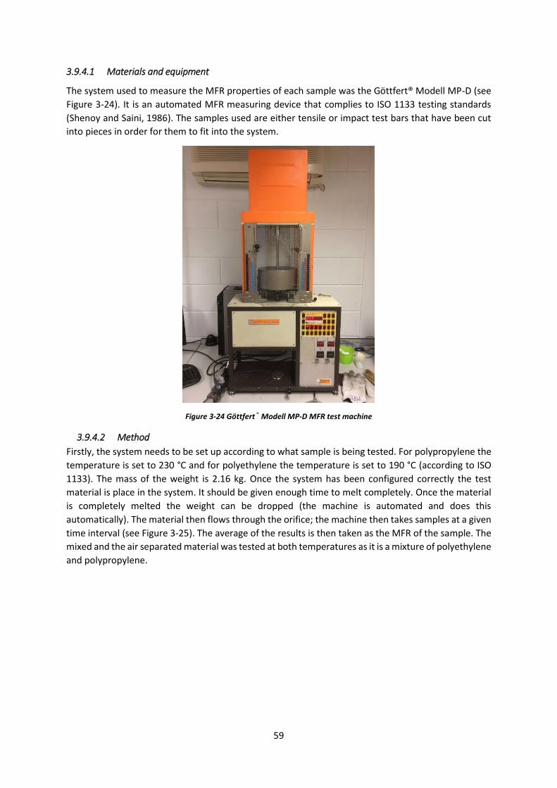
Figure 3-24 Göttfert® Modell MP-D MFR test machine ........................................................................ 59
Figure 3-25 MFR test system ................................................................................................................. 60
Figure 3-26 Mettler Toledo® DSC822 .................................................................................................... 60
Figure 4-1 Size separation mass ratio.................................................................................................... 62
Figure 4-2 Mixed sample wall thickness distribution ............................................................................ 62
Figure 4-3 HDPE BM grade sample wall thickness distribution ............................................................ 63
Figure 4-4 PP IM grade sample wall thickness distribution .................................................................. 63
Figure 4-5 HDPE BM & IM grade sample wall thickness distribution.................................................... 64
Figure 4-6 Correlation between wall thickness and polymer type ....................................................... 64
Figure 4-7 Settling velocity experiment ................................................................................................ 65
Figure 4-8 Mass fractions (mixed material)........................................................................................... 66
Figure 4-9 Mass fractions (mixed material, 5 – 11 mm)........................................................................ 66
Figure 4-10 Recovery curves (Mixed material) ..................................................................................... 67
Figure 4-11 Recovery curves (mixed, 5-11 mm) .................................................................................... 67
Figure 4-12 Herbold® testing mass measurements .............................................................................. 68
Figure 4-13 Mass measurement – feed rate comparison ..................................................................... 69
Figure 4-14 Recovery curves (Mixed, PP and HDPE material) ............................................................... 69
Figure 4-15 Recovery curves – Mixed sample (feed rate assessment) ................................................. 70
Figure 4-16 Mixed sample bulk densities .............................................................................................. 71
Figure 4-17 Ballistic testing mass measurement results ....................................................................... 71
Figure 4-18 Separation curves ............................................................................................................... 72
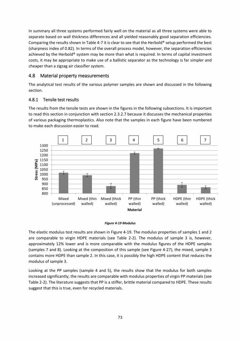
Figure 4-19 Modulus ............................................................................................................................. 73
Figure 4-20: Yield stress ........................................................................................................................ 74
Figure 4-21 Tensile stress ...................................................................................................................... 74
Figure 4-22 Tensile strain at yield ......................................................................................................... 75
Figure 4-23 Maximum tensile strain ..................................................................................................... 75
Figure 4-24 Impact resilience ................................................................................................................ 76
Figure 4-25 Melt Flow Index (ISO 1133 @ 190°C) ................................................................................. 76
Figure 4-26 Melt Flow Index (ISO 1133 @ 230°C) ................................................................................. 77
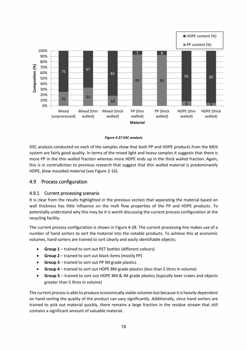
Figure 4-27 DSC analysis ........................................................................................................................ 78
Figure 4-28 Current hand sorting configuration ................................................................................... 80
Figure 4-29 proposed process configuration ........................................................................................ 81
Page 11
ix
Tables Table 1-1 sample material composition .................................................................................................. 5
Table 2-1 Density ranges of various polymers ...................................................................................... 17
Table 2-2: Mechanical properties of common polymers ...................................................................... 17
Table 2-3 MFI properties of virgin polymers ......................................................................................... 23
Table 2-4 Mechanical properties of virgin and recycled HDPE ............................................................. 27
Table 2-5 Change of properties of an HDPE part reprocessed 15 times ............................................... 27
Table 3-1 Experimental equipment ....................................................................................................... 37
Table 3-2 Test matrix ............................................................................................................................. 39
Table 4-1 Size measurement results ..................................................................................................... 61
Table 4-2 Density range measurements................................................................................................ 65
Table 4-3 Mixed material cut points and sharpness indices ................................................................. 67
Table 4-4 Mixed (5-11 mm) material cut points and sharpness indices ............................................... 68
Table 4-5 Original, P1 and P2 material cut points and sharpness indices ............................................. 70
Table 4-6 Cut points and separation indices ......................................................................................... 72
Table 4-7: Air classification results comparison .................................................................................... 72
Page 12
x
Nomenclature
Polymer – a macromolecule that is composed of a number of repeating units or monomers
Polyolefin – any polymer that is part of the alkene group
Melt Flow Index – the measure of the viscosity of a material
Virgin Polymer – primary polymer materials synthesised from hydrocarbons such as oil and gas
Plastic – the general term for polymer based products
Monomer – a molecule that has the ability to bind to other molecules
Polyethylene – a polymer derived from the ethylene monomer
Polypropylene – a polymer derived from the propylene monomer
Polystyrene – a polymer derived from the styrene monomer
Polyethylene Terephthalate – a polymer derived from the ethylene terephthalate monomer
Recyclate – recycled material
NIR spectroscopy – Near Infrared spectroscopy
Rheology – the study of the flow of materials in a liquid state
Chemical recycling – recycling by means of chemically breaking down a material into its individual
molecules and re-synthesizing them into a new material
Mechanical recycling – recycling by means of mechanical technologies
Page 13
List of acronyms
PP – Polypropylene
PE – Polyethylene
HDPE – High density polyethylene
LDPE – Low density polyethylene
LLDPE – Linear low density polyethylene
MFI – Melt flow index
MFR – Melt Flow Rate
MDS – Magnetic density separation
EU – European Union
P1 – Magnetic Density Separation polypropylene product
P2 – Magnetic Density Separation Polyethylene product
FTIR – Fourier Transform Infrared Spectroscopy
DSC – Differential Scanning Calorimetry
PS – Polystyrene
PVC – Polyvinylchloride
PET – Polyethylene Terephthalate
Page 14
1
CHAPTER 1
1 Introduction
Ever since the discovery of synthetic polymers during the early decades of the 20th century, plastics
have become an integral part of modern society. Plastics are relatively cheap, easy to manufacture and
durable making them the choice material for applications in a number of industries such as agriculture
and plastic packaging. Plastics are ideal materials for packaging applications and are used to package
almost every consumable product on the market today. This makes the plastic packaging sector the
largest plastic consumer – it accounts for 39% of the total European plastics market (Plastics Europe,
2015).
Plastic packaging products can be manufactured from a range of different plastics depending on the
intended application. Figure 1-1 outlines the most common packaging polymers and their typical
applications. The most widely used polymers in the packaging industry are Polyethylene Terephthalate
(PET), High Density and Low Density Polyethylene (HDPE & LDPE) and Polypropylene (PP).
Figure 1-1 Common packaging plastics and their associated resin codes (Ellen Mac Arthur Foundation, 2016)
Page 15
2
Despite these polymers having many favourable physical properties, the majority of packaging
products are designed for single usage after which it is subsequently discarded. The result is that plastic
packaging accounts for the majority of plastic waste ending up in the total waste stream; most of these
plastics then end up in landfills or in our natural environment with only 2% being closed-loop1 recycled
and 8% being cascade2 recycled (see Figure 1-2). The overwhelming majority of the value locked in
packaging materials is lost to the economy every year; the reclamation and recycling of these materials
is therefore becoming an increasingly important topic for many industries and governing bodies across
the globe.
Figure 1-2 Plastic packaging flows (Ellen Mac Arthur Foundation, 2016)
Plastic recycling is undertaken by one of two methods: chemical recycling or mechanical recycling.
Mechanical recycling is the favoured approach as it is less energy and cost intensive. Mechanical
recycling is the process of sorting mixed plastics into homogeneous plastic fractions so that it may be
melted and formed into new products. Referring back to Figure 1-1, resin codes3 are often imprinted
onto packaging products to assist recyclers in sorting mixed plastics into homogeneous plastic
fractions. In order to achieve closed loop recycling the purity of the recyclate should, depending on the
polymer in question, be in the order of 90% or higher.
1 Closed loop recycling is the process of using recycled materials to produce a product of a similar quality compared to the original product
2 Cascade recycling is the process of using recycled materials to produce a product of a lower quality compared to the original product
3 Resin codes refer to polymer type
Page 16
3
In conjunction with separating plastics according to polymer type, plastics need to be sorted according
to other physical properties such as colour and melt flow (rheological) properties4 to produce
recyclates that closely resemble the physical characteristics of the original or virgin material.
Viscosity, with regards to plastics, refers to the melt flow or rheological properties of a molten polymer
at a given temperature. Viscosity is an important physical property when it comes to the manufacturing
of different plastic products because different manufacturing processes, such as blow moulding and
injection moulding, require polymers with different viscosities in molten form. Typically, injection
moulding applications require polymers with low viscosities in molten form whereas blow moulding
applications require polymers that are far more viscous in molten form (see section 2.4 for more
information). If two or more different polymers with different melt flow properties are melted down
together the result is a product with melt flow properties that are not suitable to either manufacturing
process.
For all the research focused on plastic recycling, very little research has been carried out on how to
separate plastics based on their melt flow properties; more specifically, how to separate plastics that
were initially blow moulded from plastics that were initially injection moulded. In this study two
techniques were used to attempt to separate a plastic recyclate mixture into a blow mould rich fraction
and an injection mould rich fraction. After separating the material, the physical properties of each
fraction were measured to determine to what degree the physical properties and melt flow properties
were improved or worsened.
1.1 Project background
1.1.1 Magnetic Density Separation
This research was conducted in conjunction with another project that focused on sorting different
polymers according to polymer type by using a newly developed technology known as Magnetic
Density Separation. Magnetic Density Separation (MDS), developed by the European Commission
funded ‘Waste to Plastics’ project, has the proven ability to separate complex mixes of plastic waste
into a number of high quality products in a single step. One of its strong applications is the separation
of mixed polyolefin5 waste into high purity Polyethylene (PE) and polypropylene (PP) recyclates. But
to create a truly versatile recyclate the material must also be sorted according to its melt flow or
rheological properties. Figure 1-3 is a simple flow diagram of the proposed process.
Figure 1-3 Plastic separation overview (developed by author)
4 Melt flow (rheological) properties refer to the behaviour of the polymer in molten form
5 Polyolefin refers to any plastic synthesised from an alkene monomer (PP and PE are both polyolefin’s)
Page 17
4
1.1.2 Melt Flow Index
The Melt Flow Index (MFI) of a polymer is the measurement of the viscosity of a molten polymer or
the ease of flow of a molten polymer. It is defined as the mass of a molten polymer that flows, in ten
minutes, through a capillary under a specific pressure and has the units, 𝑔/10𝑚𝑖𝑛 (Shenoy and Saini,
1986). This term will be used repeatedly throughout the report when referring to melt flow
(rheological) properties.
For the purposes of this study, the two grades of plastic will be referred to as blow mould (BM) grade
and injection mould (IM) grade. BM and IM grade plastics have different MFI’s and can only be used
for either blow moulding or injection moulding applications.
1.1.3 Recycling facility
The sample material for this project was supplied by a recycling facility that is in the process of
integrating an MDS system into their recycling line. The recycling facility is located in Romania and it
currently produces four products by means of manual hand sorting, namely:
1. HDPE blow mould grade (mixed colours)
2. PP injection mould grade (black)
3. PP injection mould grade (mixed colours)
4. HDPE blow and injection mould grade (mixed colours)
Figure 1-4 is a simple process flow diagram of the operation at the recycling facility in Romania.
Figure 1-4 Recycling plant process overview (developed by author)
Page 18
5
Material sourced from municipal waste collection services enters the facility without any prior
treatment. It is fed, as is, into the primary sorting facility where the rubbish bags are opened to liberate
the contents. It passes through a series of sorters that remove most of the organic materials, non-
ferrous and ferrous metals, paper and cardboard. The pre-screened material is fed onto two conveyor
lines where hand-sorters sort out different types of plastics. The different plastics are transferred to
the secondary hand sorting facility where hand sorters manually sort the mixed into the four products
listed at the beginning of this chapter. Manual sorting the material is believed to achieve purities,
according to polymer type, of between 80 and 90%.
In order to test the MDS system a 20 tonne sample of material was prepared by the Romanian recycler
for processing. This material was also the sample material used in this investigation. The material
supplied was a mixture of three out of the four products they produce. The PP injection mould (black)
sample was not included because it was deemed unsuitable for MDS processing. The composition of
the sample material is shown in Table 1-1. The material was shredded, washed and dried before it was
mixed together.
Table 1-1 sample material composition (information supplied by Romanian recycler)
Product name Percentage of total
HDPE blow mould grade (mixed colours) 50%
PP injection mould grade (mixed colours) 33%
HDPE blow and injection mould grade (mixed colours) 17%
In addition to supplying a 20 tonne sample, the recycling company also supplied 10 kg individual
samples of the products listed in Table 1-1.
1.2 Objectives of the study
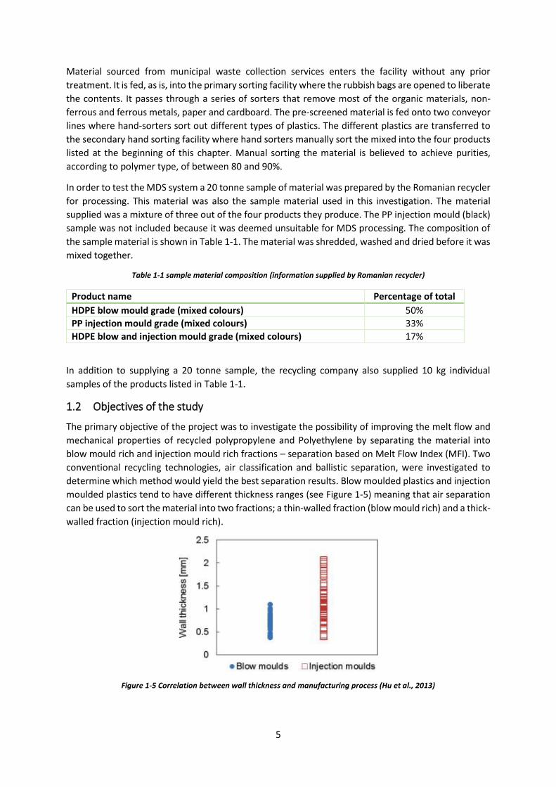
The primary objective of the project was to investigate the possibility of improving the melt flow and
mechanical properties of recycled polypropylene and Polyethylene by separating the material into
blow mould rich and injection mould rich fractions – separation based on Melt Flow Index (MFI). Two
conventional recycling technologies, air classification and ballistic separation, were investigated to
determine which method would yield the best separation results. Blow moulded plastics and injection
moulded plastics tend to have different thickness ranges (see Figure 1-5) meaning that air separation
can be used to sort the material into two fractions; a thin-walled fraction (blow mould rich) and a thick-
walled fraction (injection mould rich).
Figure 1-5 Correlation between wall thickness and manufacturing process (Hu et al., 2013)
Page 19
6
The method, or separation technology that yielded the best separation results was used to attempt to
produce blow mould rich and injection mould rich samples.
To enable this process, it was important to measure the physical characteristics (size, density and
thickness characteristics) of the material before and after separation for three purposes:
1. To determine how to optimally configure the air classification and ballistic separation systems
2. To determine mass fractions of each material before and after separation
3. To use as input information in future processing models
Once it was decided which separation technology to use, two processing configurations were
investigated; separating the different samples into a thick and thin fractions before MDS processing
(see Figure 1-6) and separating them after MDS processing (see Figure 1-7). The samples were then
processed into test samples for further mechanical and melt flow property measurements. The aim
was to be able to compare which process configuration yielded the best results; specifically, in terms
of the melt flow properties of each sample.
Figure 1-6 Pre-MDS separation
Figure 1-7 Post-MDS separation (developed by author)
The secondary objective of the research was to study the operation and performance of the chosen
separation system in more detail to understand the throughput limitations of each system if it were to
be implemented into a plastic recycling processing line (see Figure 1-8).
Page 20
7
Figure 1-8 System throughput and performance measurement (developed by author)
1.3 Scope of the study
This research focusses specifically on HDPE and PP household packaging waste. PET and other plastics
were not included in the test samples. The sample material was supplied by a single plastic recycling
facility. The focus area of the study is the European Union (EU) area (EU-27 plus Norway and
Switzerland6) because the sample material used in this investigation is from a European source.
1.4 Limitations and constraints
Although this research takes an in depth look at the different characteristics of different polyolefin
samples, it is limited to one recycling plant in one region of Romania. If this study were to be repeated
elsewhere it may yield different results.
The material samples used to conduct this research was also supplied by the recycler shredded,
cleaned and dried. The pre-treatment of this material by means of hand sorting means that certain
plastic items are intentionally left out of the mix before shredding takes place.
Furthermore, the research report only studied the properties of material samples that had been
separated into two wall-thickness ranges; 0.0 and 0.9 mm and > 0.9 mm. A more comprehensive study
could separate the material into a number of different thickness ranges to more comprehensively
understand the correlation between wall-thickness and melt flow properties.
1.5 Structure of the report
This report comprise of five chapters; Introduction, Literature review, Experimental methods, Results
and discussion and Conclusions and recommendations. A short description of each chapter is given
below.
CHAPTER 2 – Literature review
The literature review provides important information about plastics, recycling, and air separation.
CHAPTER 3 – Experimental methods
The first part of the experimental methods chapter deals with the measurement and characterization
of the plastic material. This serves as important information for the air classification part of the
investigation.
6 EU-27 plus Norway and Switzerland will be considered as Western Europe throughout this report
Page 21
8
The air classification and ballistic separation sections describe the experiments conducted on the
plastic material.
The final section focusses on the measurement of the mechanical and melt flow properties of material
samples from the air classification section.
CHAPTER 4 – Results and discussion
The results and discussion section examines the results of the research and discusses the observed
trends in the data.
CHAPTER 5 – Conclusions and recommendations of future work
This chapter provides a brief discussion and some closing remarks on the findings of the research. It
also includes a small subsection discussing the potential for further research on the topic.
Page 22
9
CHAPTER 2
2 Literature review
2.1 European polymer industry
Europe is one of the biggest producers and converters of polymers with an industry turnover of roughly
€320 billion in 2013. The industry directly employs approximately 1.45 million people across Europe,
the majority of which operate within the plastics conversion sector of the plastics industry (Plastics
Europe, 2015).
In 2013 the aggregated production of plastics in Europe was an estimated 57 Mtonne accounting for
20 % of global plastics production. The demand for plastic products within Europe was approximately
46.3 Mtonne with five countries accounting for the majority of plastics consumption: Germany, Italy,
France, the United Kingdom and Spain (Plastics Europe, 2015).
Plastics have become an integral part of nearly all industrial sectors because of their versatility,
relatively low production and manufacturing costs, and their ability to be reused through recycling or
energy generation. Plastics in Europe are used widely among a number of important markets. Figure
2-1 gives a breakdown of the European plastics market. It can be seen that the largest demand for
plastics is for application as packaging material.
Figure 2-1 Plastics demand by sector in 2013 (plastics Europe, 2015)
2.1.1 Plastic packaging
Plastic packaging accounts for approximately 39% of total plastic demand which are used for primary
(sales packaging), secondary (grouped packaging) and tertiary (transport packaging) applications
(APME, 2001). Plastics are manufactured from a variety of polymers with varying mechanical and
physical properties. Different applications require different properties such as mouldability, barriers
to moisture and other environmental elements, transparency and temperature protection (Erlov et al.,
2000). The plastics that are predominantly used for the manufacturing of packaging materials are
21,7%
4,3%
5,6%
8,5%
20,3%
39,6%
Others
Agriculture
Electrical & Electronics
Automotive
Building & Construction
Packaging
Page 23
10
polyethylene (PE), polypropylene (PP) and polyethylene terephthalate (PET). PE consumption can be
categorized further according to its specific type; low density PE (LDPE), linear low density PE (LLDPE)
and high density PE (HDPE). Other notable polymers utilized in smaller fractions are polyvinyl chloride
(PVC), polystyrene (PS) and polyurethane (PUR) (Plastics Europe, 2015). Figure 2-2 provides a
breakdown of European plastics demand by polymer type for the purposes of packaging
manufacturing.
Figure 2-2 Packaging plastics consumption by polymer type in Europe 1999 (APME, 2001)
Furthermore Figure 2-3 provides insight into exactly what these polymers are converted into and the
means by which they are manufactured.
Figure 2-3 Packaging products (APME, 2001)
2.1.2 Waste management
Plastic recycling has, since the 1980s, become an increasingly important topic for the EU as it attempts
to reduce and reuse post-consumer waste materials. Waste management remains a major challenge
0 500 1000 1500 2000 2500 3000 3500 4000 4500 5000
LDPE/LLDPE
HDPE
PP
PET
PS
PVC
EPS
Other Thermoplastics
Thermosets
(x 1000 tonnenes/year)
Packaging polymers
0 500 1000 1500 2000 2500 3000 3500 4000
Films
Hollow pieces
Sacks & bags
Injection moulded products
Thermoformed products
Foams
Other (extrusion, laminates)
(x 1000 tonnenes/year)
Packaging products
Page 24
11
for Europe and as a result the EU has developed a general waste management hierarchy for EU
member states to follow (Gascoigne and Oglivie, 1995):
Prevent wastes generation at the source
Reuse the materials through recycling and energy generation
Effectively dispose of waste residues that cannot be reused
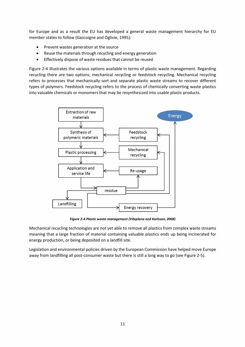
Figure 2-4 illustrates the various options available in terms of plastic waste management. Regarding
recycling there are two options; mechanical recycling or feedstock recycling. Mechanical recycling
refers to processes that mechanically sort and separate plastic waste streams to recover different
types of polymers. Feedstock recycling refers to the process of chemically converting waste plastics
into valuable chemicals or monomers that may be resynthesized into usable plastic products.
Figure 2-4 Plastic waste management (Vilaplana and Karlsson, 2008)
Mechanical recycling technologies are not yet able to remove all plastics from complex waste streams
meaning that a large fraction of material containing valuable plastics ends up being incinerated for
energy production, or being deposited on a landfill site.
Legislation and environmental policies driven by the European Commission have helped move Europe
away from landfilling all post-consumer waste but there is still a long way to go (see Figure 2-5).
Page 25
12
Figure 2-5 European landfill scenarios (Plastics Europe, 2015)
2.1.3 Plastic recycling
Sorting and recycling of complex polymer waste streams remains a difficult and costly process and is
the reason why only a small fraction of post-consumer plastics are recycled. The value of the recyclate
is also lower than the value of the virgin material7. Manufacturing processes, exposure to the elements
and mixing different types and grades of polymers renders a secondary material with inferior
properties compared with virgin polymers. Virgin polymers used by plastics converters generally
conform to strict product standards that ensure the finished products adhere to standards imposed by
standards authorities, manufacturers and consumers of products packaged in plastics. In addition to
product quality, manufacturing machinery require polymers that adhere to strict technical
specifications to guarantee desired operational performance. In most cases recyclates do not meet the
required specifications for the production of most primary packaging products.
Additionally, it is mostly the easy-to-sort materials that are fully recycled such as PET bottles and plastic
drinks crates because of their homogenous nature and ease of identification by conventional recycling
technologies. Other plastic packaging materials are more difficult to sort. Many packaging products
that look similar may indeed be manufactured from different polymers or may contain additives and
pigments that make them non compatible with one another; the recycled product therefore does not
resemble the quality of the virgin material (Luijsterburg and Goossens, 2014). Subsequently, the
market value of recyclates is significantly lower than virgin polymers because the value of recyclates
are directly linked to the market value of virgin polymers.
The European Commission is aware of the problem and understands the scale of the value locked in
packaging waste. As a result, the European commission has provided funding for a number of projects
aimed at increasing the fraction of plastics that are recycled. Additionally, they want to establish a
circular economy whereby materials that are recyclable are reused several times for the same purpose
thus reducing the demand for virgin polymers.
7 Commonly referred to as downcycling or cascade recycling; the value of the recyclate is lower than the value of the original product
Page 26
13
One of the projects funded by the European Commission’s FP7 programme (titled “W2Plastics8”) has
developed a unique and powerful technology that has the ability to separate a complex polyolefin flake
stream by polymer type in one step: Magnetic Density Separation (MDS) is able to sort these complex
waste streams into attractive secondary products of high quality and in economically feasible volumes
(Serranti et al., 2015).
2.2 Magnetic Density Separation
Magnetic Density Separation (MDS) is a specialized method of separating polymer flakes according to
their density. Different polymers have different densities; separating on density thus separates
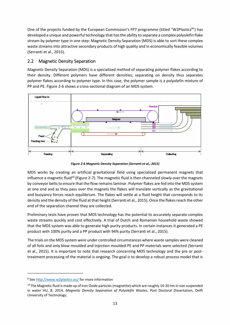
polymer flakes according to polymer type. In this case, the polymer sample is a polyolefin mixture of
PP and PE. Figure 2-6 shows a cross-sectional diagram of an MDS system.
Figure 2-6 Magnetic Density Separation (Serranti et al., 2015)
MDS works by creating an artificial gravitational field using specialized permanent magnets that
influence a magnetic fluid10 (Figure 2-7). The magnetic fluid is then channeled slowly over the magnets
by conveyor belts to ensure that the flow remains laminar. Polymer flakes are fed into the MDS system
at one end and as they pass over the magnets the flakes will translate vertically as the gravitational
and buoyancy forces reach equilibrium. The flakes will settle at a fluid height that corresponds to its
density and the density of the fluid at that height (Serranti et al., 2015). Once the flakes reach the other
end of the separation channel they are collected.
Preliminary tests have proven that MDS technology has the potential to accurately separate complex
waste streams quickly and cost effectively. A trial of Dutch and Romanian household waste showed
that the MDS system was able to generate high purity products. In certain instances it generated a PE
product with 100% purity and a PP product with 94% purity (Serranti et al., 2015).
The trials on the MDS system were under controlled circumstances where waste samples were cleaned
of all foils and only blow moulded and injection moulded PE and PP materials were selected (Serranti
et al., 2015). It is important to note that research concerning MDS technology and the pre or post-
treatment processing of the material is ongoing. The goal is to develop a robust process model that is
8 See http://www.w2plastics.eu/ for more information
10 The Magnetic fluid is made up of Iron Oxide particles (magnetite) which are roughly 10-20 nm in size suspended in water HU, B. 2014. Magnetic Density Separation of Polyolefin Wastes. Post Doctoral Dissertation, Delft University of Technology.
Page 27
14
able to separate complex polyolefin waste streams into high purity products quickly and cost
effectively.
Figure 2-7 Density gradient of magnetic fluid in the presence of a magnet (Hu, 2014)
2.3 Polymers
Polymers have become an integral material in modern society with plastics being used for various
applications in a number of industries ranging from consumer goods to building and construction. The
unique range of physical properties and relatively low costs attributed to polymers makes them a
versatile group of materials for both manufacturers and designers.
2.3.1 Types of polymers
Polymers are either referred to as natural or synthetic polymers. Natural polymers are materials such
as starch, rubber and cellulose and occur naturally whereas synthetic polymers (the focus material for
this report) refer to all polymers that have been synthesized from feedstocks such as crude oil.
Synthetic polymers are more commonly referred to as plastics and are divided into two main groups:
thermoplastics and thermosetting plastics. Thermoplastics account for approximately 80% of total
plastic consumption because of their durability and manufacturing versatility (Biron, 2012).
Thermoplastics soften when heated and solidify when cooled and undergo a physical transformation
that is reversible. Thermoplastics are suited for recycling applications because the process of softening
and solidifying may be repeated without compromising the mechanical and chemical integrity of the
plastic (Biron, 2012); however, if thermoplastics are exposed to high temperatures, for instance well
above the melting temperature of a specific thermoplastic, it may lead to degradation of the polymer
(Callister, 2007).
Examples of common thermoplastics are polyethylene (PE), polypropylene (PP), polyvinyl chloride
(PVC) and polystyrene (PS). PE (of differing densities), PP, PS and PVC make up 70% of total plastics
production because of their relatively low costs, durability and versatility that make them ideal for
plastic packaging applications (Xanthos, 2005).
Page 28
15
Thermosetting plastics refer to the group of polymers that are liquid at low temperatures and as they
solidify they undergo a chemical reaction that is irreversible. Once they have taken their desired form
they cannot be reheated or melted and formed into another shape. Examples of thermosetting plastics
are polyurethanes and epoxy resins. This group of plastics remains challenging to recycle because it is
not possible to melt and reform them again (Biron, 2012). For recycling purposes, only thermoplastics
are considered in this investigation; it is therefore important to understand the physical and chemical
properties of different thermoplastics.
2.3.2 Properties of thermoplastics
2.3.2.1 Polymer molecules
Polymers are groups of simple monomers such as ethylene or propylene that bond together during the
reaction in the presence of an initiator and a catalyst. Figure 2-8 illustrates the transformation from an
ethylene monomer to ethylene polymer. The polymer molecule in Figure 2-8 is the repeating unit in a
particular polymer chain. Polymer chains can vary in length but still have the same repeating unit;
paraffin wax and polyethylene are both made from ethene but have very different chain lengths giving
each very different mechanical properties (Blackman et al., 2012).
Figure 2-8 Ethylene transformation to polypropylene (University Of Cambridge)
2.3.2.2 Molecular weight
Molecular weight is an important property of a polymer. Molecular weight or molecular mass refers
to the length of a polymer chain; the longer the polymer chain, the higher the molecular weight. During
polymerization polymer chains grow to different lengths depending on the process itself and the
intended application of the polymer. As a general rule the melt transition temperature of a polymer
increases as the length or molecular mass of the polymer chain increases. Mechanical properties also
depend on the molecular mass of a polymer; elastic modulus and tensile strength increases as
molecular mass increases (Callister, 2007).
2.3.2.3 Molecular shape and structure
The molecular shape of a polymer is an important property as a number of characteristics of the
polymer depend on the shape of the polymer. Because single chain bonds have the ability to rotate in
three dimensions, a polymer chain can bend and twist entangling itself into something that resembles
a bowl of spaghetti. This property allows a certain degree of rotational flexibility making the polymer
tougher. Polymers with double carbon bonds or large side groups tend to have a higher rotational
rigidity making them more brittle (Sivasankar, 2008).
Page 29
16
The structure of a polymer refers to the manner by which polymer chains join together. Figure 2-9
shows common polymeric structures; linear, branched, cross-linked and network structures.
Figure 2-9 Polymer structures (Adapted from Callister, 2007)
The structure of a polymer is a characteristic of the polymer that develops during its synthesis.
Different processes are designed to achieve certain polymer structures in order to produce a material
with desired properties and characteristics such as density and tensile strength. Polypropylene and
polystyrene are linearly structured whereas polymers such as Polyethylene (LDPE and HDPE) are
branched polymers (Callister, 2007).
2.3.2.4 Polymer crystallinity
Crystallinity in any material refers to the ordering of the molecules of a specific material in its solid
phase. Metals are a good example of crystalline materials as they are almost always crystalline in solid
phase. Polymers, however, have a more complicated structure in solid form. The relative size and
complexity of polymer molecules means that crystallization is only possible under certain conditions.
To achieve crystallinity, polymer melts need to cool slowly allowing time for the polymer chains to
align themselves into a lattice configuration. Linearly structured polymers are fairly easy to crystalize
because there are few restrictions to alignment whereas branched polymers have significant
restrictions making it more difficult for polymer chains to align (Callister, 2007).
Most polymers are therefore semi crystalline; polymers with crystalline regions embedded in the
amorphous phase of the polymer. Crystallinity may have an influence on the mechanical and physical
properties of a specific polymer; polymers with a high crystallinity are generally stronger and more
resistant to heat and dissolution (Callister, 2007).
2.3.2.5 Stereoisomers
Stereoisomers refers to monomer molecules that have the same formula that are joined together
uniformly from head to tail but differ in their three dimensional arrangement. Three spatial
configurations are possible: isotactic, syndiotactic and atactic (see Figure 2-10).
Typically, a given polymer is not defined or characterized as having a single configuration; the
configuration of a polymer is usually a combination of the above with the dominant configuration
resulting from the method of synthesis (Callister, 2007).
Page 30
17
Isotactic configuration: R groups11 on the same side of the
chain
Syndiotactic configuration: R groups on alternate sides of
the chain
Atactic configuration: randomly ordered R groups
Figure 2-10 Tacticity (Adapted from Callister, 2007)
2.3.2.6 Polymer densities
Understanding the density differences between different thermoset plastics is important because a
number of mechanical recycling techniques rely on the plastics density for separation. It should also
be noted that manufacturers are moving towards using plastics of lower densities for economic
reasons (World Economic Forum, 2016) Table 2-1 lists the densities the various polymers.
Table 2-1 Density ranges of various polymers adapted from (Mark, 2007)
Chemical name Density (𝒌𝒈/𝒎𝟑)
Low density polyethylene (LDPE) 910 – 925 Linear low density polyethylene (LLDPE) 918 – 935 High density polyethylene (HDPE) 941 – 965 Polyethylene terephthalate (PET) 1330 – 1420 Polyporopylene (PP) 850 – 920 Polystyrene (PS) 1040 – 1090 Polyvinyl Chloride (PVC) 1300-1450
2.3.2.7 Mechanical properties
Polymers can have very different mechanical properties depending on their molecular structure.
Plastic packaging polymers need to be tough and ductile to ensure they do not fracture or tear. Other
applications, such as computer keyboards, require a material that is harder and stiffer than flexible
polymers. The mechanical properties of the typical packaging polymers of are listed in Table 2-2.
Table 2-2: Mechanical properties of common polymers adapted from (Callister, 2007)
Material Elastic Modulus
(𝑮𝑷𝒂) Yield Strength
(𝑴𝑷𝒂) Tensile Strength
(𝑴𝑷𝒂) Percent
Elongation
LDPE 0.172-0.282 9.0-14.5 8.3-31.4 100-650
HDPE 1.08 26.2-33.1 22.1-31.0 10-1200
PET 2.76-4.14 59.3 48.3-72.4 30-300
PP 1.14-1.55 31.0-37.2 31.0-41.4 100-600
PS 2.28-3.28 - 35.9-51.7 1.2-2.5
PVC 2.41-4.14 40.7-44.8 40.7-51.7 40-80
11 R groups refer to any atom or side group other than Hydrogen
C C
H
H
H
R R
H
H
H
CC
R
H
H
H
CC
R
H
H
H
CC
C C
H
H
H
R
C C
H
H
H
R
C C
H
H
H
R R
H
H
H
CC
C C
H
H
H
R R
H
H
H
CC
R
H
H
H
CC
R
H
H
H
CC
Page 31
18
2.3.3 Virgin polymer production
Synthetic polymers are polymers whose chemical makeup is based on the carbon atom. Synthetic
polymers are therefore mostly synthesized from natural resources such as coal, natural gas and crude
oil. The process of polymer manufacturing begins by separating the hydrocarbons from the raw
material input. Once the desired hydrocarbons have been extracted they are then converted into
monomers such as ethylene or propylene through a process commonly known as cracking (Chauvel
and Lefebvre, 1989). In this form, the individual monomers can be chemically bonded into chains
through one of two basic mechanisms: condensation or addition reactions (Ghosh, 2001).
Condensation reactions are chemical reactions where two monomers join together to form a larger
molecule with a smaller molecule being eliminated. Condensation reactions are used to produce
materials such as polyamides, polyesters, polycarbonates and polyurethanes; typically, thermoset
plastics. Addition reactions are chemical reactions where monomer units bond together without the
elimination of any atoms. Addition reactions are used to produce materials such as polyethylene and
polypropylene; typically, thermoplastics (Blackman et al., 2012).
2.3.3.1 Polyethylene production
Addition reactions are used to manufacture PE and are carried out in the presence of a catalyst. LDPE
is produced in the presence of peroxide catalysts whereas Ziegler-Natta12 systems are common
commercially used systems for the production of HDPE (Blackman et al., 2012).
LDPE has a density range between 910 and 925 kg/m3 with a melt transition temperature of
approximately 115°C. LDPE has a lower density compared to HDPE as a result of the chains of LDPE
being highly branched. As a result, LDPE cannot be used in applications where it is exposed to
temperatures in excess of its melt transition temperature. 65% of LDPE is used for the manufacturing
of films for the packaging of consumer goods (Blackman et al., 2012).
HDPE is a much stronger material than LDPE with a density range of approximately 941 to 965 kg/m3
and a melt transition temperature of approximately 133°C. The improved strength comes from the fact
that HDPE is more crystalline than LDPE; less branching yields a material that is far more crystalline
with stronger intermolecular forces. HDPE is used in applications where strength is important such as
bottles, bottle caps, rigid food packaging containers and hard hats (Blackman et al., 2012).
2.3.3.2 Polypropylene production
polypropylene is also the product of an addition reaction where the asymmetric propene alkene is
polymerized. Since propene is asymmetrical its polymerization may result in three types of
polypropylene associated with the arrangement of its ethyl branch; isotactic polypropylene,
syndiotactic polypropylene and atactic polypropylene. Isotactic polypropylene is the type of
polypropylene that exhibits desirable commercial properties. It is produced in the presence of a
modified Ziegler-Natta catalyst and results in a material with high strength and stiffness (Blackman et
al., 2012). As a result, PP tends to be stiffer, and more rigid than HDPE (Ghosh, 2001).
2.3.4 Polymer additives
Additives play an important role in polymer manufacturing. Additives refer to any material or
compound that is added to the polymer mix that modify its properties. Additives include fillers,
colorants, stabilizers and plasticizers. Additives for plastic recycling purposes are beneficial as certain
types of additives have the ability to improve the recyclability of a polymer (AlMaaded et al., 2014).
12 Ziegler-Natta catalysts are Titanium based catalysts used to support addition reactions.
Page 32
19
Additives are also used for cosmetic reasons such as pigments that give a particular plastic object a
desired colour.
2.3.4.1 Fillers
Fillers refer to organic or inorganic particles or fibres ranging from nanoparticles to continuous fibres
of varying shapes and profiles that are added to a given polymer during manufacturing. One of the
primary reasons for adding fillers is to reduce the overall volume fraction of the more expensive
polymer; this makes manufacturing cheaper as less polymer material is used (Xanthos, 2005). Fillers
can also be added to reinforce a polymer; adding fillers can help to increase the modulus and strength
of a polymer (La Mantia, 1998b). If improved electrical or thermal conductivity properties are required,
the addition of a conductive filler may help to improve these properties. The addition of fillers can
assist in manufacturing; certain fillers can help to prevent warpage during manufacturing (Xanthos,
2005).
Fillers are mostly used for plastics in the following industries: building and construction, automotive
and consumer goods. Packaging materials do not usually contain fillers. Fillers do, however, play an
important role in plastic recycling. Fillers can be added to recycled PP to improve the elastic modulus
and tensile strength (La Mantia, 1998a); however, in terms of density separation, the presence of fillers
can have a negative impact. Fillers change the density of a polymer; exploiting the density differences
of a recyclate mix is no longer possible if the densities are modified.
2.3.4.2 Colourants
Colourants are added to plastics to change their colour, mostly for aesthetic purposes. Colourants are
typically organic and inorganic pigments or synthetic dyes but significant progress has been made
regarding the development of polymeric colorants (Miley, 1996). The appropriate type of colorant
needed depends on the application of the plastic object; certain dyes are toxic making them unsuitable
for food packaging, however, dyes and pigment colorants are still used in packaging materials raising
questions as to the safety of such practices (Robertson, 2012).
In terms of mechanical properties, the addition of colorant additives does not have significantly
adverse effects. In a study focusing on PP it was found that, in some instance, the addition of organic
and inorganic pigments actually improved the Elastic Modulus and Tensile Strength (Kanu et al., 2001).
However, colourants create a significant challenge when it comes to plastic recycling. Recycling
different coloured plastics together renders a grey coloured product which limits its commercial
versatility.
2.3.4.3 Stabilizers
Polymers in general are often susceptible to degradation when exposed to heat or ultraviolet light
during manufacturing or exposure to sunlight (Hinsken et al., 1991). To prevent or hinder degradation,
stabilizers - such antioxidants or UV absorbers - can be added to the polymer. In some instances,
stabilizers are added to monomers to prevent premature polymerization during the conversion of
monomers to a polymer.
Stabilizers are important additives regarding plastic recycling. Repeated processing can lead to
considerable chain scission increasing the Melt Flow Index (MFI) of the recyclate (La Mantia, 1998a).
Chain scission can be reduced by adding a stabilizer before each recycling step (see Figure 2-11).
Stabilizers are therefore important additives concerning the recycling of polyolefin’s.
Page 33
20
Figure 2-11 Impact of stabilizers on recycled PP - Adapted from (La Mantia, 1998a)
2.3.4.4 Compatibilization
Polymers of different types have different properties defined by an array of characteristics unique to
each polymer; density, molecular characteristics, polarity and degree of crystallinity to name a few.
The unique characteristics of different polymers also dictate their degree of compatibility or miscibility
if blended with another polymer or group of polymers. Polymers are said to be miscible if they
resemble a single phase material in solid phase and immiscible if they separate into phases of the
individual fractions of each original polymer (Robeson, 2007).
Polymers made up of combinations of different polymers are known as polymer blends. Polymer
blends are produced because they often have superior mechanical and physical properties compared
to the original constituents. An example of a commercial polymer blend is Nyrol® that was developed
in the 1960s by General Electric. Nyrol® is a poly(2,6-dimethyl-1,4-phenylene oxide)-polystyrene blend
and is used in electronics, and coating applications. It has a higher glass transition temperature than
its individual constituents as well as improved impact resistance and tensile strength (Robeson, 2007).
Compatibilization refers to the practice of processing immiscible polymers in such a way that they
resemble a single phase material in solid state. There are two main compatibilization practices: block
or graft copolymer addition and reactive compatibilization (Robeson, 2007).
Block or graft copolymer addition refers to the process of adding a copolymer to a binary polymer
blend in order to lower the interfacial tension between each phase. Lowering the interfacial tension
between each face improves adhesion between each phase, stabilizing its morphology and improving
its mechanical properties (Robeson, 2007).
Reactive compatibilization is the practice of creating a continuous single phase polymer blend between
two highly immiscible polymers by adding a reactive polymer to the mix. The reactive polymer is
miscible with one of the polymers in the blend and reactive to certain functional groups on the other
polymer. It leads to the formation of in-situ graft or block copolymers that reduce interfacial tension
and improve dispersion leading to an improvement in mechanical properties (Robeson, 2007).
Polymer compatibilizers are especially important when it comes to plastic recycling. Post-consumer
packaging waste is a complex mixture of a number of different types of plastic; most of which are
immiscible in one another. Separating complex mixes of post-consumer waste into “pure” fractions of
each type of polymer remains challenging and even the smallest amount of contaminant material can
compromise the properties of the recyclate. Compatibilizers therefore make it possible to recycle
different polyolefin’s together to render a recyclate with acceptable mechanical properties.
0
1
2
3
4
5
6
0 1 2 3 4 5
MFI
(g/
10
min
)
Number of extrusions
Unstabilized PP
Stabilized PP
Page 34
21
2.4 Rheology of plastics
Rheology is the science of the flow of matter in molten form or as a soft solid that deform plastically
instead of elastically under the influence of an applied force. The applied force can be compressive,
tensile, torsional, shear or a combination of all four resulting in a specific type of flow. For the purposes
of this report only shear flow (see Figure 2-12) and extensional flow (see Figure 2-13) will be considered
as these are the fundamental flow mechanisms regarding injection moulding and blow moulding
applications (Wilkes, 1981)
2.4.1 Shear flow
The shear force acting on a polymer melt results in the chains of the polymer to slide past one another.
The degree to which these layers deform relative to on another is known as shear strain and is denoted
as the symbol 𝛾 = 𝑋 𝑌⁄ (Figure 2-12). The rate at which these layers slide past one another is termed
the shear rate and is usually denoted as the symbol �� = 𝑑𝛾 𝑑𝑡⁄ (𝑠−1) (Wilkes, 1981).
Taken one step further the resistance to fluid flow can be described by its viscosity and is often denoted
by the symbol, 𝜂. Viscosity is a function of the applied shear force and the shear rate, 𝜂 = 𝜏 ��⁄ (𝑃𝑎 ∙ 𝑠)
which is a linear function. It is important to note that polymer melts deviate from this rule and are
categorized as non-Newtonian fluids when in molten form (Wilkes, 1981).
Figure 2-12 Deformation by shear - adapted from (Wilkes, 1981)
2.4.2 Extensional flow
Extensional flow is the result of a polymer melt experiencing elongation in molten form during
processing. Extensional flow is either uniaxial, biaxial or planar (Figure 2-13) in nature depending on
the forces acting on the polymer (Aho, 2011).
Page 35
22
Figure 2-13 Extensional flow of a polymer melt - adapted from (Aho, 2011)
2.4.3 Viscosity and Melt Flow Index (MFI)
The viscosity of a polymer melt is dependent on a number of factors and can be categorized as being
either external or internal factors. External factors refer to variables that act on a particular polymer
such as temperature, pressure and time. Internal factors refer to properties intrinsic to the polymer
such as molecular weight, molecular shape and molecular architecture (Wilkes, 1981).
The Melt Flow Index (MFI) of a polymer is the measurement of the viscosity of a molten polymer or
the ease of flow of a molten polymer. It is defined as the mass of a molten polymer that flows, in ten
minutes, through a capillary under a specific pressure and has the units, g/10 min. The apparatus used
to test for MFI is known as an extrusion rheometer (Shenoy and Saini, 1986).
2.4.3.1 Standardised MFI testing – ISO 1133-1:2011
The standard test used by most polymer manufacturers and converters for testing the MFI of a given
polymer is the ISO 1133-1:2011 international standard. The standard is used to test both PE and PP
polymer types. It is a simple process of heating the polymer (190°C for PE and 230°C for PP) for a set
time and then forcing it under a standard mass (usually 2.16kg) through a die of standard length and
cross-sectional area and profile. After a set period of time a sample is taken to be weighed (Shenoy
and Saini, 1986).
2.4.4 Manufacturing and recycling considerations
The internal factors of a virgin polymer are synthesized and manipulated to render a product with
specific mechanical and rheological properties suited for various applications and manufacturing
processes. Concerning manufacturing type, different grades of polymers are used for different
applications. Injection moulding requires low viscosity (high MFI) raw materials whereas blow
moulding requires high viscosity (low MFI) raw materials. For injection moulding and extrusion
applications shear thinning rheological properties are exploited whereas extensional rheological
properties are exploited for secondary processing applications such as blow moulding (Aho, 2011).
Page 36
23
2.4.4.1 Virgin polymer melt flow properties
Polymer producers manufacture various polymers for use by plastics converters who process virgin
polymers into usable products such as drink bottles and food packaging. Different applications require
polymers suited for the application and the manner in which the product is manufactured; in this case
either injection or blow moulded. Many commercial polymer producers therefore have extensive
polymer product ranges suited for a number of uses and processing applications. Focusing on melt
flow properties most polymer producers offer a variety of products with different melt flow properties
suited to a specific manufacturing application. Table 2-3 gives MFI information for virgin polymers
manufactured by three major virgin polymer producers in Europe.
Table 2-3 MFI properties of virgin polymers (generated by author)
Application Total Basell Orlen Chevron Phillips
Injection mould grade 2.0-110 4.0-100 4.5-35
Blow mould grade 0.2-20 0.3-6.5 0.3-2.0 Note: All values are standard MFI units (g/10min) tested using the ISO 1133 testing procedure
Table 2-3 clearly shows the correlation between MFI (or viscosity in molten form) and manufacturing
process. Polymers with higher MFI’s are generally better suited to injection moulding applications
whereas polymers with lower MFI’s are generally better suited to blow moulding applications. There
is, however, an overlap where polymers can be used for both manufacturing processes. Depending on
the sophistication of the manufacturing equipment and the type of product being manufactured, a
given polymer may be used for blow and injection moulding purposes; however, this study attempts
to determine by what factor the BM and IM fractions can be improved.
2.5 Plastic packaging characterisation
Since the discovery of polymers mid-way through the 20th their use has become ubiquitous in modern
society. The unique and diverse range of mechanical, thermal and manufacturing properties of
polymers (specifically polyolefin’s such as PE and PP) make them the ideal raw materials for the
production of plastic packaging products; plastic packaging’s account for almost 40% of the plastics
market share (Hu et al., 2013).
Unfortunately, most of these plastic packaging materials are used once before being discarded - after
the product inside the packaging has been removed it is usually disposed of along with other plastics
or waste materials (depending on the waste disposal legislation and infrastructure of a given region).
The value of plastic packaging waste materials is largely lost because only a small fraction of the total
waste stream is effectively recycled and reintroduced into the market. This is changing as a result of
clear directives from the European Union regarding the recovery and reuse of waste materials by
means of reuse and recycling.
Recycling is an obvious solution; however, it has its own set of fundamental challenges. Part of the
challenge regarding plastic recycling is the separation of a mixed waste stream into homogeneous
fractions. In order to realize the full economic value of waste plastics it is important to understand the
composition and characteristics of the waste stream. New and existing technologies exploit a number
of intrinsic polymer properties in order to sort them according to type and colour; by understanding
the physical and geometrical characteristics of the waste stream, new and conventional recycling
technologies and processes may be optimized to achieve good separation.
Page 37
24
2.5.1 Density distribution
One of the most important characteristics of a polyolefin, and key to the success of Magnetic Density
Separation, is the density-type correlation of common polyolefin’s. A study looking at Romanian
household waste clearly identified the correlation between density and plastic type: PP is concentrated
in the density range between 880 kg/m3 and 920 kg/m3, whereas the density range of PE (specifically
HDPE) is between 930 kg/m3 and 980 kg/m3 (Hu et al., 2013). Figure 2-14 illustrates the density range
of PP and PE for Romanian household waste.
Figure 2-14 Density distribution of Romanian PP and PE (Hu et al., 2013)
2.5.2 Rheological properties
As discussed in previous sections rheological properties are an important parameter when it comes to
the processing of a polymer into a usable product; typically, blow moulded polymers have a higher
viscosity than injection moulded polymers. What is also clear is that it is important to try and separate
waste plastics based on viscosity or Melt Flow Index (MFI) to render a recyclate with the rheological
properties that resemble that of a virgin material. This may prove possible as there is a clear correlation
between mold type, polymer type and wall thickness distribution (Hu et al., 2013).
2.5.2.1 Polymer type correlation
According to the same study investigating the characteristics of Romanian packaging waste it was
found that there was a strong correlation between polymer type and mould type. Figure 2-15 shows
that injection moulded plastics are mostly PP (>80%) whereas blow moulded plastics are mostly PE
(>80%) (Hu et al., 2013).
2.5.2.2 Wall thickness correlation
The correlation between wall thickness and mould type is somewhat self-evident. Blow moulded
plastics are typically fairly thin in comparison to injection moulded plastics. There is however an
overlapping region where the thicknesses of blow moulded and injection mould plastics match.
Referring again to the study focused on Romanian household packaging waste this assumption was
verified by measuring the wall thickness of plastics known to be either blow or injection moulded (see
Figure 2-16) (Hu et al., 2013).
Page 38
25
Figure 2-15 Mould type – polymer type correlation (Hu et al., 2013)
Figure 2-16 Thickness distribution of Romanian blow mould and injection mould plastics (Hu et al., 2013)
2.6 Mechanical recycling
Mechanical recycling of plastic packaging waste is a process involving a number of steps13 that clean
and sort different polymers according to type, colour, density and rigidity. Each step in the process is
conducted mechanically and no chemical change of the polymer takes place during the process. The
goals of mechanical recycling facilities are to sort different plastics (in this case polyolefin’s, PP and
HDPE) into cleaned, uncontaminated, homogeneous material streams that are suitable to be
processed into new products (see Figure 2-17).
Mechanical recycling is conducted using a number of systems and technologies from rudimentary hand
sorting lines to more sophisticated Near Infrared (NIR) spectroscopy14 sorting systems. Most
mechanical recycling plants are integrated process lines that take advantage of a number of
technologies and processes to optimally sort different plastics into homogeneous streams.
Manufacturing purely homogeneous polyolefin waste streams are possible but difficult to achieve with
current technologies; the vast number of different grades, types and colours of plastic packaging
materials in circulation makes it a complex task.
13 Different recyclers have different process lines tailored to the material they are processing
14 NIR spectroscopy sorting exploits the near-infrared spectral fingerprint of different plastics to sort them by resin type.
Page 39
26
Figure 2-17 Mechanical recycling scenario - Adapted from (Rajendran et al., 2013)
Aside from sorting the waste stream into homogeneous fractions, the challenge remains that the
polymer, once processed into a recycled granulate, may not exhibit the same molecular, mechanical
and physical properties as exhibited by the virgin material. A number of factors are at play when it
comes to the degradation of a polymer - processing conditions, exposure to heat and ultraviolet light
during its lifetime and chemical attack are some of the mechanisms that lead to degradation of the
polymer. The quality of the recyclate is also affected by the amount of contamination of one type of
polymer in another (see 2.3.4.4 regarding polymer compatibility): in the case of Polyethylene
Terephthalate (PET) recycling, small amounts of polyvinyl Chloride (PVC) contamination may have
severe impacts on the quality of a recyclate (La Mantia, 1996).
The following sections address the topics surrounding polymer degradation and the challenges and
opportunities surrounding mechanical recycling.
2.6.1 Polymer degradation
Recyclers are constantly improving their processes and technologies in order to improve the quality of
the recyclate to be used for an increasing number of applications. The end goal is to be able to use the
same material for the same application a number of times while minimizing waste residues and the
reliance on virgin materials. The challenge remains that, no matter how careful the manufacturing
process or how sophisticated the disposal and collection system is, the polymer will inevitably become
compromised by one or other mechanism. This is known as polymer degradation and is precipitated
by a number of factors at different points in a product’s lifecycle (La Mantia, 1996).
2.6.1.1 Processing conditions
Polymer parts (plastic packaging specifically) are generally formed under high pressures and
temperatures. Injection moulding forces molten plastic into a particular die under high temperatures
and pressures to ensure that it fills the mould entirely. Blow moulded and sheet formed parts are also
processed under high temperature and pressure conditions. Heat during processing is particularly
harmful to the integrity of the polymer; melting the polymer often leads to chain scission of the
polymer (causing a reduction in molecular weight) and the formation of crosslinking and branched
polymer groups changing its mechanical properties (La Mantia, 2002). Mechanical force has also been
observed to result in chain scission during processing (Allen and Edge, 1992). A study comparing the
Page 40
27
mechanical properties of virgin and recycled HDPE found that the secondary material’s mechanical
properties indeed differed from the virgin materials properties (see Table 2-4).
Repeated processing also impacts the quality of a polymer; degradation increases as the number of
processing cycle’s increases. Table 2-5 shows how, after 15 processing cycles, an HDPE fuel tank’s
mechanical properties have reduced. Multiple reprocessing also leads to a decrease in the viscosity of
a polymer by the reduction of molecular weight caused by chain scission after each processing cycle
(see Figure 2-11).
Table 2-4 Mechanical properties of virgin and recycled HDPE - adapted from (La Mantia, 2002)
Property Virgin HDPE Recycled HDPE
Modulus (MPa) 596 640
Tensile strength (MPa) 33.7 34.2
Elongation at break (%) 69.7 36.9
Impact strength (N) 135 120
Table 2-5 Change of properties of an HDPE part reprocessed 15 times - adapted from (La Mantia, 2002)
Property Change in each property, %
Modulus of elasticity -8.2
Yield stress -3.0
Elongation at yield -20.7
Processing of virgin materials and reprocessing of recycled materials is therefore a common cause for
the degradation of a polymer’s mechanical properties. Fortunately, a number of additives designed
specifically to counter the effects of repeated processing are widely available to plastic converters and
recyclers (see section 2.3.4).
2.6.1.2 Environmental attack
All plastic packaging materials come into contact with an environmental element at some point during
their lifecycle; be it exposure to ultraviolet light, heat, moisture, oxygen, chemical and biological
compounds, an applied force or a combination of a number of these elements. Each element has the
ability to attack a given polymer causing some degree of chain scission, crosslinking or oxidation
degrading the polymer to some extent (Allen and Edge, 1992).
In terms of recycling environmental degradation only complicates the matter further. Since products
enter the environment at different times and are exposed to different elements for varying lengths of
time it is difficult to anticipate the degree of degradation of a given polymer. Blending a mixture of
used plastic packaging material therefore renders a complex product of different materials yielding a
product with variability in terms of mechanical properties. Again, the use of additives plays an
instrumental role in the recycling of plastics into usable products with good mechanical properties.
2.6.1.3 Mixing and composition
Mixing and reprocessing different types of plastics often leads to a reduction in performance of desired
mechanical properties because the polymer blend is most likely incompatible. Most polymer blends
tend to be immiscible in one another meaning that at the molecular level there is typically a clear
interface between the two polymers which usually translates into poor or less than desirable
mechanical properties (Eastwood et al., 2005).
Page 41
28
2.7 Fundamentals of particles in a fluid flow
For the purposes of this research project air classification is the mechanism by which particles of
varying thickness15 are to be separated. Before air classification can be discussed the fundamentals of
particles in a fluid flow is discussed.
2.7.1 Shape considerations
The majority of research covering particles in a fluid flow deals with particles that have been
considered spherical in shape for ease of analysis and calculation. This is not a satisfactory approach
as the geometric profile of a particle in question may significantly influence the way in which it behaves
in a fluid flow (Concha and Barrientos, 1986). It must also be noted that the flow regime (transitional
or turbulent) also affects irregularly shaped particles differently to spherically shaped particles (Tran-
Cong et al., 2004).
It is therefore important to give the particles in question some form of general classification. Plastic
flakes between 12-14mm have varying dimensions and thicknesses. If the shape is not satisfactorily
defined by approximating it to a flat cylinder it may be classified as being axisymmetric and orthotropic
and can be described graphically as follows (Clift et al., 1978):
Figure 2-18 Ellipse for representing approximate dimensions of a particle (Clift et al., 1978)
Where 𝐸 = 𝑏/𝑎, and 𝐸 → 0 for disks as the spheroid becomes increasingly oblate. The shape of the
particle becomes increasingly important as the Reynold’s number of the fluid flow increases.
Irregularly shaped particles generally undergo rotational and translational motion during their fall
through a fluid. The translational coefficient of drag and Reynolds number is related to the surface of
the particle that moves parallel to the surface plane of the particle. The rotational motion, however, is
related to the dimensionless moment of inertia described by (Clift et al., 1978):
𝐼∗ = 𝜋𝛾𝛿/128𝑎 (Equation 1)
Where:
𝐼∗ = 𝐷𝑖𝑚𝑒𝑛𝑠𝑖𝑜𝑛𝑙𝑒𝑠𝑠 𝑚𝑜𝑚𝑒𝑛𝑡 𝑜𝑓 𝑖𝑛𝑒𝑟𝑡𝑖𝑎
𝛾 = 𝐷𝑒𝑛𝑠𝑖𝑡𝑦 𝑟𝑎𝑡𝑖𝑜
𝛿 = 𝑇ℎ𝑖𝑐𝑘𝑛𝑒𝑠𝑠 𝑜𝑓 𝑑𝑖𝑠𝑘
𝑎 = 𝑅𝑎𝑑𝑖𝑢𝑠 𝑜𝑓 𝑑𝑖𝑠𝑘
15 The assumption is that particles will be separated based on thickness
Page 42
29
2.7.2 Internal flow through a duct
Air classifiers are typically ducts of a specific cross-sectional geometry, length and longitudinal profile
(either constant or changing along the length of the classifier). It is important to understand the
dimensions of the classifier as it will have influence on the flow characteristics at different velocities.
The Reynolds number is the non-dimensionalized number that traditionally describes the nature of the
fluid flow. The Reynolds number can be described as (White, 2008):
𝑅𝑒 =𝑉𝐿
𝜈 (Equation 2)
Where:
𝑉 = 𝑓𝑙𝑢𝑖𝑑 𝑣𝑒𝑙𝑜𝑐𝑖𝑡𝑦
𝐿 = 𝑙𝑒𝑛𝑔𝑡ℎ 𝑜𝑓 𝑡ℎ𝑒 𝑐ℎ𝑎𝑛𝑛𝑒𝑙
𝜐 = 𝑘𝑖𝑛𝑒𝑚𝑎𝑡𝑖𝑐 𝑣𝑖𝑠𝑐𝑜𝑐𝑖𝑡𝑦 – for air at 20 degrees Celsius is 1.5×10⁻⁵ m2/s (White, 2008)
Generally, the Reynolds number corresponds to a specific flow regime. The kinematic viscosity and the
velocity of the air flow for this investigation means that the flow regime is most likely turbulent where
there is a slight Reynolds number dependence (White, 2008):
104 < Re < 106 - turbulence, moderate Reynolds number dependence
106 < Re < ∞ - turbulence, slight Reynolds number dependence
2.7.3 Particles in a fluid flow
Particles immersed in a fluid are acted on by three forces; the force of weight induced by gravity, drag
induced by the viscosity of the fluid, and buoyancy induced by fluid displacement. The viscosity of the
fluid creates shear forces on the surfaces of a particle leading to a drag force as the particle moves
through a fluid. At low velocities this is known as viscous resistance and at high velocities it is known
as turbulent resistance (Wills, 2011). The magnitude of the resistance of the immersed particle in a
flowing fluid is influenced by a number of factors associated with the particle itself, and the fluid it is
immersed in. In terms of the fluid that the particles are immersed in, the parameters that influence
their movement are (Taggart and Behre, 1945):
The flow velocity and direction
The pressure and any pressure gradients within the fluid
The viscosity of the fluid
The temperature and humidity of the fluid
Investigating the manner in which a particle or a collection of particles of the same or differing size
behave in a fluid flow is a complex science that requires the use of a combination of fluid dynamics,
numerical modelling and experimentation and is beyond the scope of this project.
2.7.4 Terminal (settling) velocity of a particle in the presence of buoyancy force
The terminal or settling velocity of particles in a fluid flow is the velocity at which the drag force and
force of gravity equate one another resulting in the particle falling at a constant velocity. Depending
on the velocity of the fluid flow the particles will either sink or become entrained in the flow depending
on the velocity of the fluid flow and the settling velocity of the particles (Wills, 2011). In terms of
separation, heavy particles will continue to fall under their weight despite being in the presence of an
air flow flowing in the opposite direction. The lighter particles, having a lower settling velocity than
Page 43
30
their heavier counterparts, become entrained in the flow and exit the classifier in the opposite
direction.
2.7.4.1 Basic physics
If a particle falls through a fluid under its own weight it reaches terminal velocity when the weight of
the particle is balanced by the sum of the drag and buoyancy forces (Brown and Lawler, 2003):
𝑊 = 𝐹𝑑 + 𝐹𝑏 (Equation 3)
Where:
𝑊 = 𝑤𝑒𝑖𝑔ℎ𝑡 𝑜𝑓 𝑡ℎ𝑒 𝑝𝑎𝑟𝑡𝑖𝑐𝑙𝑒
𝐹𝑑 = 𝑑𝑟𝑎𝑔 𝑓𝑜𝑟𝑐𝑒
𝐹𝑏 = 𝑏𝑢𝑜𝑦𝑎𝑛𝑐𝑦 𝑓𝑜𝑟𝑐𝑒
Furthermore:
𝑊 = 𝜋𝑎2𝛿𝜌𝑠𝑑2𝑦
𝑑𝑡2 (Equation 4)
𝐹𝑑 = 𝐶𝑑1
2(
𝑑𝑦
𝑑𝑡)
2𝜋𝑎2 (Equation 5)
𝐹𝑏 = 𝜌𝑓𝑑2𝑦
𝑑𝑡2 𝜋𝑎2𝛿 (Equation 6)
2.7.4.2 Analytical approximation
It is important to consider the mechanism by which particles are separated. The air flow velocity and
particle density are important considerations in terms of balancing the forces of buoyancy, weight and
friction. Equation 3 simply defines the relationship between these forces and the settling velocity at
which these forces balance (Tomas and Gröger, 2001):
𝑣𝑠𝑖𝑛𝑘2 =
2
𝐶𝑑.
𝜌𝑠−𝜌𝑓
𝜌𝑓.
𝑉𝑝
𝐴𝑝. 𝑔 (Equation 7)
Where:
𝑣𝑠𝑖𝑛𝑘 =𝑑𝑦
𝑑𝑡= 𝑠𝑒𝑡𝑡𝑙𝑖𝑛𝑔 𝑣𝑒𝑙𝑜𝑐𝑖𝑡𝑦
𝑔 =𝑑2𝑦
𝑑𝑡2= 𝑔𝑟𝑎𝑣𝑖𝑡𝑎𝑡𝑖𝑜𝑛𝑎𝑙 𝑓𝑜𝑟𝑐𝑒
𝐴𝑝 = 𝑠𝑖𝑑𝑒 𝑓𝑒𝑑 𝑐𝑟𝑜𝑠𝑠 𝑠𝑒𝑐𝑡𝑖𝑜𝑛𝑎𝑙 𝑎𝑟𝑒𝑎
𝐶𝑑 = 𝑑𝑟𝑎𝑔 𝑐𝑜𝑒𝑓𝑓𝑖𝑐𝑖𝑒𝑛𝑡
𝑉𝑝 = 𝑝𝑎𝑟𝑡𝑖𝑐𝑙𝑒 𝑣𝑜𝑙𝑢𝑚𝑒
𝜌𝑓 = 𝑓𝑙𝑢𝑖𝑑 𝑑𝑒𝑛𝑠𝑖𝑡𝑦
𝜌𝑠 = 𝑑𝑒𝑛𝑠𝑖𝑡𝑦 𝑜𝑓 𝑡ℎ𝑒 𝑠𝑜𝑙𝑖𝑑 𝑝𝑎𝑟𝑡𝑖𝑐𝑙𝑒𝑠
Equation 7 is a simplification of the force balance of the forces described by Equations 4 – 6. This
equation defines a specific settling velocity based on a particles terminal velocity in an air flow. It is a
simple analytical solution that may be used to quickly approximate the settling velocity of a particle. It
Page 44
31
is a rudimentary analytical solution and does not accurately describe the settling velocity of an
irregularly shaped particle in an air flow (Tran-Cong et al., 2004).
2.7.5 Ballistic trajectory
The ballistic trajectory or trajectory of a projectile is considered the path that a particle follows after it
has been launched by an external force and acted on by an aerodynamic drag component. In the case
of material separation ballistic trajectories of different particles can be exploited in order to separate
based on particle mass and geometric profile.
To determine the distance travelled of a given particle in the presence of air resistance, Newton’s
second law is applied and solved for displacement as a function of mass and geometric profile (focusing
on horizontal movement) (Bedford and Fowler, 2007):
Σ𝐹𝑥 = −𝐹𝑎𝑖𝑟 = 𝑚𝑎𝑥 (Equation 8)
Where:
𝐹𝑎𝑖𝑟 = −𝑘𝑣 (assuming direct proportionality between air resistance and velocity)
Where 𝑘 =1
2𝜌𝑓𝐴𝐶𝑑
Integrating the second order equation:
𝑠𝑥 = 𝑚𝑘⁄ 𝑣𝑥 (1 − 𝑒−
𝑘
𝑚𝑡) (Equation 9)
Equation 9 describes the relationship between mass and displacement of the ballistic trajectory of a
particle in the presence of air resistance. As the mass of a particle increases, so does its displacement
(assuming the geometric profiles remain the same) (Bedford and Fowler, 2007).
2.8 Air classification
2.8.1 Introduction
Air classification is the process of separating particles in an air flow according to the particles settling
velocity, which is a function of the particles size, shape and weight. Air classifiers are either static or
dynamic in the way that they function (Altun and Benzer, 2014). Static air classifiers do not have any
moving parts whereas dynamic classifiers have a rotating plate onto which the material is fed,
imparting a centrifugal force on the particle to assist in separation.
Air classifiers are further defined by the characteristics of the air flow through the system. The fluid
flow through an air classifier is dependent on the geometric profile of the classifier and whether the
air flow velocity is varied or kept constant (Everett and Peirce, 1990). The composition, particle size
range, and relative particle geometry will have an influence on what type of air classifier would be best
suited to separate polyolefin flakes of differing thickness and density. Air classification separates
material based on one of these parameters meaning that all other parameters should be kept constant
to limit the influence of other variables (Tomas and Gröger, 2000)
Typically air classification has been used to separate particles according to particle size rather than
sorting a binary mix into two distinct fractions (Taggart and Behre, 1945). Air classification takes
advantage of the aerodynamic profile of a particle; perfect separation is not possible for a material
feed of particles that differ in shape, size and density (Stessel and Pelz, 1994). Each product from an
air classifier will have a degree of contamination.
Page 45
32
2.8.2 Types of separation zones
The design of an air classifier depends on the type of material that is to be separated. The separation
zone of a classifier is the area where separation occurs. The most common separation zone types are
(Shapiro and Galperin, 2005):
o Gravitational counterflow
o Gravitational crossflow
o Centrifugal counterflow
o Centrifugal crossflow
o Cascade classifiers
Cascade classifiers are best suited for the application in question and are discussed in further detail.
2.8.3 Cascade (Zigzag) air classifiers
Cascade air classifiers refer to air classifiers that are constructed from a series of rectangular ducts
joined together at a specific angle (Figure 2-19. a). The configuration can be slightly adjusted as is
shown in Figure 2-19. b, where angled plates are used to create a zigzag profile. The system can also
be used in parallel with horizontal scavenging to improve the cut efficiency (Figure 2-19. c) (Shapiro
and Galperin, 2005).
The purpose of introducing a zigzag profile is to create vortices in the flow where coarse particles are
captured, thrown to the opposite side of the separation chamber and fall to the bottom of the
classifier. Zigzag classifiers have two distinct flow streams; a stream of particles that moves upwards
and one that moves downwards at the lower point of each section (Senden, 1980). Cascade classifiers
are best suited for this application because of their superior separation sharpness compared to other
conventional air classifiers.
Cascade classifiers improve separation but increase operating costs. Cascade classifiers consume large
amounts of energy because of the pressure drop they have to overcome as a result of the zigzag profile
creating a large pressure drop over the channel.
Figure 2-19 Cascade classifiers, (a) zigzag, (b) shelf, (c) horizontal scavenging (Shapiro and Galperin, 2005)
Page 46
33
Figure 2-20 Cross section and velocity profile of a typical zigzag air classifier (Rosenbrand et al., 1986)
2.8.3.1 Experimentation with zigzag classifiers
In experimentally studying the sharpness of particle separation for a number of varying configurations
it was found that (Rosenbrand et al., 1986):
The separation sharpness between classifiers of 90 deg. And 120 deg. Were roughly the same
but the capacity of the 120 deg. Classifier was larger
If the classifier channel is broadened the separation sharpness decreases but the capacity
increases. This is the same result if the feed point is closer to one of the classifiers exit points
Wall roughness plays a role in affecting the efficiency of the system by affecting the
interactions of the falling particles with the lower zigzag walls of the separators
2.8.3.2 Particle behavior inside zigzag air classifiers
Particle-particle interactions increase as the feed rate increases. When the feed rate increases particles
interactions with other particles and the air classifiers walls increases rendering separation less
efficient (Rosenbrand et al., 1986).
Transit times of the particles also vary. Heavier particles tend to move downwards in a constant path
quicker than the lighter particles moving upwards. The lighter particles also do not follow a constant
path profile compared to the heavier particles (Rosenbrand et al., 1986)
Page 47
34
2.8.3.3 Zigzag air classifier cut points and performance
Any air classification process is utilised to separate a mixed input material into two or more products
(in this case it is a light and a heavy fraction). Air classification is not capable of perfect separation
meaning that there will always be some amount of contamination of each product fraction in the other.
The point at which the material has a 50% probability of either ending up in the heavy or light fraction
is referred to as d(50%) and it is linked to the size or thickness of the particle (depending on what
parameter the separation is based on). Therefore the d(50%) point is calculated to determine the cut
point meaning that material smaller will most likely end up in the light fraction and material larger will
most likely end up in the heavy fraction.
The efficiency of an air classifier can be measured in a number of ways. The first method discussed is
based on the masses of the different fractions entering and exiting the air classifier and is considered
the general efficiency of an air classifier. The general efficiency equation for air classifiers is given as
(Everett and Peirce, 1990):
𝐸 = √𝑥𝑒
𝑥𝑜.
𝑦𝑟
𝑦0. 100 (Equation 1)
Where 𝐸 = efficiency; 𝑥𝑒 = mass of light particles exiting as lights through the top of the classifier; 𝑥𝑜
= mass of light particles entering the classifier; 𝑦𝑟 = mass of heavy particles exiting as heavies through
bottom of classifier; 𝑦0 = mass of heavy particles entering the classifier.
An important finding was the basis on which the performance of a zigzag separator is measured. If
separation is based on efficiency of separation (defined by equation 1) then performance is
independent of particle size of the feedstock. If, however, performance is based on operating range
(defined by equation 2 where 𝑂𝑅 refers to the operating range of the classifier, 𝑓1 refers to recovery
as a percentage and 𝑓2 refers to contamination as a percentage):
𝑂𝑅 = ∫[𝑓1(𝑥) − 𝑓2(𝑥)]𝑑𝑥 (Equation 2)
then particle size affects performance. To improve operating range, the input particle size should be
small. The operating range also increases with the increase in number of zigzag stages and stage angle
(Peirce and Wittenberg, 1984).
Another measure of the performance of air classifiers is the sharpness index, s. The sharpness index is
the ratio of the d(25%) and d(75%) probabilities and it represents the sharpness of separation; 𝑠 =
𝑑(75%) 𝑑(25%)⁄ It is calculated independent of the mass of each fraction entering and exiting the air
classifier making it suitable for measuring the efficiency of the classifier without knowing the mass of
each fraction before and after air classification. Perfect separation is represented by 𝑠 = 1 but most
classifiers have sharpness indexes between 0.5 and 0.8 (Klumpar et al., 1986).
In terms of the performance of gravitational-counterflow versus zigzag classifiers, zigzag classifiers are
known to have a lower diffusivity (higher efficiency – Equation 1) than gravitational-counterflow
classifiers (Biddulph and Connor, 1989).
2.8.3.4 Effect of feed rate and classifier height on air classifier performance
Findings from research showed that tall passive-pulse stacked triangle air classifiers perform better
than tall active pulse and nonpulse air classifiers. The study also found that increasing the feed rate
also decreased the efficient separation range. Increasing the height of the classifier also showed that
it improved the effectiveness of the separation (Hagemeier et al., 2014).
Page 48
35
Air classifier performance has also been found to be dependent on the moisture content of the
feedstock (Crowe and Peirce, 1988). This is important to note; the plastic feedstock that is to be
separated must be cleaned and dried to prevent moisture content impacting air classifier efficiency.
2.9 Literature summary
The most relevant aspects to take note of before progressing to the next chapter are:
Polymer densities (section 2.3.2.6): important information for section 3.5.3 and 4.3
regarding the density measurements of the plastic samples
Polymer mechanical properties (section 2.3.2.7): important information for sections
3.9 and 4.8 regarding the mechanical properties of the plastic samples
Characteristics of plastic packaging (section 2.5): important information for sections
3.5.2, 3.6 and 3.7 regarding the correlations between wall thickness and injection and
blow moulded plastic packaging materials
Characteristics of plastic packaging (section 2.5): important information for sections
3.5.2, 3.6 and 3.7 for air classification purposes
Air classifier cut points and performance calculations (section 2.8.3.3): important
information for sections 3.7 and 3.8 regarding air classification and ballistic separation
performance calculations
Page 49
36
CHAPTER 3
3 Experimental methods
This chapter provides a detailed description of the equipment, experimental setup and methodology
applied to carry out each part of the investigation. The aim of the research is to determine, using
conventional recycling technologies, whether or not it is possible to separate blow moulded (BM) from
injection moulded (IM) plastics or vice versa using air classification or ballistic separation techniques.
As stated in previous sections and in previous studies it has been shown that BM and IM plastics have
different thickness ranges providing a parameter that may be exploited in pursuit of separating BM
and IM plastics.
3.1 Overview
The flow diagram of the experimental section is shown in Figure 3-1.
Figure 3-1 Overview of experimental method
Before the air classification and ballistic separation experiments could be carried out, the physical
characteristics (wall thickness ranges, size ranges and settling velocity) of the test samples had to be
measured. After each sample was separated into two fractions, the new samples were processed into
test bars for analysis of mechanical and melt flow properties. The Melt Flow Index (MFI) measurements
indicate whether or not sorting on wall thickness affects the melt flow properties of a recyclate by
comparing the MFI values of each sample before and after separation.
3.2 Experimental equipment
The experimental equipment used for this research is listed in Table 3-1.
Page 50
37
Table 3-1 Experimental equipment
Equipment Description Measurement range Measurement uncertainties
Vernier caliper Used to measure material wall thickness
0.00 − 150𝑚𝑚 ±0.01𝑚𝑚
Hydrometer Used to measure liquid density
0.800 − 1.000 (specific gravity)
±0.002
Mass scale Used to measure sample mass
0.00 − 3.00 kg ±0.01 g
Drying oven Used to dry wet samples
Vibrating screen Used to sieve samples
Stopwatch Used for timing purposes
±0.2𝑠
Digital impeller anemometer
Measure air flow velocity
1.00 − 30.0 m/s ±0.20 m/s
Stopwatch Used to measure drop test time
±0.2 s
Nihot air classifier Used for air classification experiments
No measurement device
Herbold air classifier Used for air classification experiments
No measurement device
Note: Uncertainties were disclosed on the technical data sheet of each piece of equipment and are at a confidence level of
95%.
The equipment used to measure various parameters were sufficiently accurate with the required
measurement resolutions for the purposes of this research.
3.3 Results
To validate the results of the research, the mechanical and melt flow properties of each tested sample
are compared with the properties of virgin polymers outlined in the literature as the aim is to produce
a recyclate with similar properties to that of the virgin material. The results are also compared with
samples that were not processed by means of air classification on density separation to determine, to
what degree, each sample was upgraded or worsened.
The performance of the air classifiers is also validated by comparing the separation efficiency results
with the results of previous studies outlined in the literature.
Page 51
38
3.4 Description of the plastic samples
3.4.1 Pre-Magnetic Density Separation (MDS) samples
The material used to conduct this research was supplied by a Romanian plastic recycling company that
produces four distinct packaging recyclates:
HDPE blow mould grade (mixed colours)
PP injection mould grade (black) – Not included in sample
PP injection mould grade (mixed colours)
HDPE blow and injection mould grade (mixed colours)
The sample that was prepared for testing excluded the PP injection grade (black) product because it is
deemed an inferior product and not suitable for MDS processing. To produce the products listed above,
a team of hand sorters sort through piles of mixed plastics that have been separated from other
materials such as metals, organic materials and paper.
The first group of hand sorters are trained to sort out all plastic bottles (mostly HDPE blow mould
bottles with injection moulded PP lids and caps) into a separate bunker. The result is a predominantly
HDPE blow mould grade product containing small amounts of PP injection mould grade plastics. The
second group of hand sorters are trained to sort out all plastic food containers (mostly PP injection
moulded food containers with a small amount of HDPE injection moulded food containers) into a
separate bunker. The third group of hand sorters are trained to sort out all the large plastic items such
as water drums and drinks crates (a mixture of blow and injection grade HDPE) into a separate bunker.
Hand sorting is able to produce products with a purity of between 80 and 90%.
For MDS testing and for this investigation, a 20 tonne sample (a mixture of the three products with a
composition corresponding to the ratio outlined in Table 1-1) was supplied by the Romanian recycling
company. In addition to the mixed material sample, 10 kg samples of the recycling plants current
products as shown in Table 1-1 were also supplied. The size, density and thickness distributions of each
of these samples was measured.
Figure 3-2 is an image of the material. It is important to note that the material is irregular in shape and
size as a result of the shredding process. For the purposes of the MDS test investigation, the material
had to be screened to a nominal size of -10 mm to ensure that it did not cause blockages in the system.
The oversized fraction was then re-shredded and mixed back into the mixed sample to avoid changing
the composition of the material. Five samples in total were measured for size, thickness and density:
Mixed sample
Mixed sample (< 10 mm)
HDPE blow mould (BM) grade (mixed colours)
PP injection mould (IM) grade (mixed colours)
HDPE blow and injection mould (BM + IM) grade (mixed plastics)
Page 52
39
Figure 3-2 Material sample
3.4.2 Test matrix
Section 3.5 describes the tests that were conducted on the different samples described above. The
matrix shown in Table 3-2 outlines which tests were conducted on which samples.
Table 3-2 Test matrix
Sample Size measurements
Thickness measurements
Density measurements
Polymer type/thickness
Mixed sample X X X
Mixed sample (< 𝟏𝟎 𝒎𝒎) X X X
HDPE BM grade X X X
PP IM grade X X X
HDPE BM + IM grade X X X
Sized samples (section 3.5.1) X X
3.4.3 Post-Magnetic Density Separation (MDS) samples
This project was done in conjunction with the MDS project and it was important to also conduct tests
on the products from the MDS system to determine whether upgrading before or after MDS was
possible. The MDS system has the ability to sort a mixture of PP and HDPE into products with a purity
in excess of 90% (Serranti et al., 2015).
Two samples of each product from the MDS project were collected for use in this investigation; a PP
product with a purity of approximately 90% and an HDPE product with a purity of approximately 95%.
3.5 Physical characterization of the material
A complete analysis of the material samples received from the recycling plant in Romania was
undertaken to understand what is possible in terms of separation; especially separation based on the
wall thickness of the material. Specific techniques were used to measure the size, thickness and density
distributions of each sample.
Page 53
40
3.5.1 Size measurements
Each of the five samples described in section 3.4 were separated into different size fractions to
determine the composition of each sample in terms of size. The size of the material is an important
parameter with regards to air classification as the drag of a particle immersed in a fluid is a function of
the surface area of a particle. Particles with a large surface area generate more drag than particles
with a small surface area. To separate the material based on wall thickness alone the settling velocity
of each particle, influenced by surface drag forces, should be limited (see section 2.7).
In the case of the material needing to be sorted into different size ranges for air classification purposes,
it is important to understand the fraction of each size range for throughput calculations of the recycling
system as a whole.
3.5.1.1 Method
The distribution of particle sizes of each sample were determined by separating the material into
different size fractions (approximately 0-5 mm, 5-11 mm, > 11 mm) using a laboratory stacked
vibrating screen machine with 4 𝑚𝑚 and 8 𝑚𝑚 square sieves (Figure 3-4). Figure 3-3 shows how
material larger than 4 𝑚𝑚 and 8 𝑚𝑚 is able to pass through these square sieves.
The sieves were stacked with the larger grid size on top. Approximately 1 kg of material, considered a
representative sample without overloading the screens, was placed on the top grid before the vibrator
was sealed. The vibrator then vibrated the material until it was completely separated into different
size fractions (each sample was processed for enough time to ensure complete separation). Each
fraction was removed, weighed and weight recorded. This process was repeated for each sample (see
Table 3-2). See appendix 1 for a step by step procedure.
Figure 3-3 Square grid dimensions
Page 54
41
Stacked vibrating screen Square sieves
Figure 3-4 Apparatus for size measurement tests
3.5.2 Thickness measurements
The thickness distribution measurements are used to help determine the separation cut points when
attempting to separate thin-walled from thick-walled plastics. The thickness distribution
measurements also given an indication of the expected masses of each fraction after they have been
separated into a thin-walled and thick-walled fraction. Additionally, it also becomes a useful tool when
calculating the separation curve charts of air classifiers and ballistic separators (see section3.7). The
thickness distributions were measured for all the samples (see Table 3-2).
3.5.2.1 Method
Thickness measurements were conducted by measuring the wall thickness of individual plastic flakes
from each sample using a vernier caliper. The measurements were recorded and translated into
histograms that graphically display the thickness distribution of each sample. Each column in the
histogram represents a thickness interval of 0.1 mm. See appendix 2 for step by step procedure.
3.5.2.2 Correlation between wall thickness and polymer type
Previous research has suggested that different categories of products are made from different
polyolefins; blow moulded plastic bottles are generally made from HDPE and injection moulded
plastics are generally made from PP (Hu et al., 2013). It was therefore worth investigating the
relationship between wall thickness and polymer type. From the same mixed sample used in section
3.5.2, the type of polymer of each flake was recorded using a technique known as Fourier Transform
Infrared (FTIR) spectroscopy.
Page 55
42
FTIR spectroscopy is a technique that measures how much light (at different frequencies) is absorbed
by the sample at which the light is directed (Griffiths and de Haseth, 2006b). The “Fourier Transform”
part of the name refers to the exploitation of the mathematical process that converts the raw data
into a readable spectrum (Griffiths and de Haseth, 2006a). Once a sample’s infrared profile has been
analyzed, the system determines the composition of the material by matching it to known materials in
the laboratories self-populated database. A PerkinElmer Spectrum FT-IR spectrometer was used for
this investigation.
3.5.3 Density measurements
The density distribution for each sample was assessed to determine the mass fractions of PP and HDPE
in each of the samples outlined in Table 3-2. A series of simple sink-float tests were undertaken to
separate each sample according to the density of HDPE and PP in each sample. Once completed the
ratio of each density fraction was calculated.
3.5.3.1 Method
The method used to determine the density distributions of each sample was the same method used in
a study that did a similar density distribution analysis on packaging waste material (Hu et al, 2012).
Firstly, two solutions of water and pure propanol were prepared so that one solution had a density of
920 kg/m3 and the other 930 kg/m3. Material that lighter than 920 kg/m3 is regarded as PP and material
heavier than 930 𝑘𝑔 𝑚3⁄ is regarded as HDPE (see section 2.3.2.6). Sink float tests were conducted
on each sample using the solutions described above to separate the material into three density
fractions: < 920 kg/m3, 920 to 930 kg/m3, > 930 kg/m3. See appendix 3 for a step by step procedure.
3.5.4 Bulk density measurements
The bulk density of the material represents the mass of the material per volume. It is not an intrinsic
property of the material but rather a measure of how much mass of a specific material occupies a given
volume. It is important to understand the bulk density of the material as it has implications when
determining the economic aspects of a process.
The purpose of the bulk density measurements for this study was to show that bulk density varies
according to material wall thickness. The bulk densities of the material before and after air
classification were measured for comparison (see section 3.7 regarding air classification).
There are a number of standardized measuring methods for measuring bulk density; mostly oriented
to soils and powders (materials of relatively small grain size). For the purposes of this study the bulk
density of each material was measured using a simple metal tray and an electronic scale.
3.5.4.1 Method – bulk density measurement
For the bulk density measurement, material is placed into a tray of known volume (6092 cm3) and
weighed. The mass of the material in the tray is then divided by the volume to give the bulk density.
This procedure was repeated for each sample.
3.6 Settling velocity measurements
The settling velocity of a particle immersed in a fluid defines the point at which the forces of gravity,
buoyancy and frictional drag are balanced. The result is that the particle falls at a constant velocity
under free fall or remains somewhat stationary when placed in an air flow stream. The force balance
that describes settling velocity explains that settling velocity is a function of a number of properties of
both the particle in question and the fluid into which it is immersed. Particle shape, size, density, profile
Page 56
43
and surface roughness, and liquid viscosity and density all influence the settling velocity (see section
2.7).
To accurately calculate or compute the settling velocity of irregular particles is challenging and
subsequently falls outside of the scope of this project; however, it is possible to experimentally
determine the settling velocities of a number of different plastic particles. Because the material is not
homogeneous in terms of shape and size, a number of plastic flakes of different size and shape were
included in the experiment. What is most important is to determine how the settling velocity changes
as the wall thickness of the material changes.
The settling velocity experiment was conducted with material from the mixed sample. The settling
velocity was determined by using two different methods:
dropping individual particles from a height
constructing a simple air flow chamber that particles can be immersed in
Each method will be discussed individually. For both experiments the same plastic flakes were used in
order to compare the results directly.
3.6.1 Material preparation
The thickness and size of individual flakes were measured and the general shape of the flake recorded
for each particle from a representative sample of the mixed material. After measurement each flake
was placed in a container that corresponded to its thickness. Flake thickness varied from 0.51 to 1.64
mm.
Once a sufficient number of particles had been measured and separated according to thickness, each
thickness batch was further sorted down to 5 particles, each having a different shape and size as shown
in Figure 3-5.
Figure 3-5 Settling velocity flake selection
3.6.2 Settling velocity determination – Drop test
After measurement and sorting a flake was dropped from a height 4.19 m (the height between ground
level and the first floor at the laboratory) with all the doors and windows nearby closed. The time taken
for the plastic flake to hit the ground was recorded. This step was repeated for each flake.
3.6.3 Settling velocity determination – Flow chamber
The experimental setup for the settling velocity measurements in a laboratory flow chamber is given
in Figure 3-6. The flow chamber was a square Perspex air channel with dimensions 45 by 48 mm. A
digital impeller anemometer and a flow meter were used to record the air velocity.
To carry out the experiment a single plastic flake was first placed in the flow chamber. The pressure
valve was then slowly opened to allow air to flow through the chamber. The valve was opened
incrementally until the particle began to gently flutter. The volumetric air flow rate and anemometer
Page 57
44
readings were recorded. The average air velocity was calculated for plastic flakes that fell into the same
wall thickness range.
Figure 3-6: Flow chamber setup
3.7 Air classification
Air classification was carried out on the mixed sample material to determine how efficiently the
material could be separated into two fractions; one resembling thin-walled (blow mould rich) material
and the other resembling thick-walled (injection mould rich) material. The air classification
investigation was conducted on (see section 3.4 for more information):
Mixed sample material (< 10 mm)
Polypropylene material – MDS product
Polyethylene material – MDS product
Mixed sample material (5-10 mm)
The first round of air classification tests was carried out on a Nihot® WS-Z zigzag classifier. The focus
of the first round of tests was to determine:
the effect of air flow rate on the separation cut point,
what cut points (in terms of wall thickness) were possible on a typical zigzag air classifier setup,
the corresponding masses of each fraction for each experiment,
the correlation between particle surface area differences and separation efficiency (see
section 2.7 for more information)
Page 58
45
The second round of air classification tests was conducted on a more advanced air classification
system; the second machine, A Herbold® SZS 630/212 zigzag air classifier, had a much taller zigzag
separation chamber, frequency controlled fans and a frequency controlled vibrating feeder. The
Herbold® configuration was not as powerful as the Nihot® setup but more precise control of the feed
rate and air flow rate was possible. The purpose of the second round of testing was:
to determine the whether there is a correlation between classifier height and separation
efficiency
to determine effect of feed rate on separation efficiency
3.7.1 Material preparation
3.7.1.1 Mixed material
Mixed material was included in the air classification investigation to determine whether or not it would
make practical sense to place the air classification step before density separation (see Figure 3-7). Air
classification was also carried out to determine by how much the material can be upgraded before
being separated by the MDS system. It also serves as a point of reference for comparison with
separation of the MDS PP and HDPE products.
Figure 3-7 Air classification before polymer type separation
3.7.1.2 PP and HDPE MDS products
Air classification on the MDS PP and HDPE products may prove to yield higher quality IM and BM
products. The mixed material sample is a polyolefin mix made up of three streams of material
produced by Romanian processing plant; it is a mixture of IM grade PP, BM grade HDPE and an IM-BM
HDPE mixture (see section 3.4). The MDS system has the ability to separate this material into a PP rich
fraction and a HDPE rich fraction. If this information is accurate it means that the PP product is already
a product which is an injection mould rich product and the HDPE product is an IM-BM mixture (see
Figure 3-8). Air classification could prove to be a refining step that upgrades the product further after
MDS processing.
Page 59
46
Figure 3-8 MDS processing
3.7.1.3 Mixed material (5-11 mm)
This sample was included in the study to determine the impact flake size has on separation efficiency.
By reducing the nominal size range, it is believed that separation based on wall thickness would
improve as the influence of another variable, flake surface area, is reduced.
Before testing each material sample had to be prepared, packaged and labelled. The mixed material
did not require any screening or washing; it was simply weighed, packaged and labelled accordingly.
The 5 − 10 𝑚𝑚 sample had to be prepared by sieving mixed material (20 kg sample) using a vibrating
screen. Once enough material was screened it was weighed, packaged and labelled.
PP and HDPE (MDS products) material had to be washed and dried before weighing and packaging. A
sample of PP was taken from a batch that corresponded to a PP quality of 90%. The material was then
washed in cold water and drained to remove all residual magnetic fluid. The material was then dried
by spreading it out over a plastic sheet to speed up the drying process. Once dried it was weighed,
packaged and labelled. HDPE material was prepared in the same way as PP material.
3.7.2 Nihot® Amsterdam WS-Z zigzag air classifier
The Nihot® WS-Z air classifier is a typical zigzag air classifier (see Figure 3-9). Material is fed into the
top of the zigzag channel by a vibrating screen where initial separation occurs. The light material
immediately becomes entrained in the airflow and is removed from the top of the chamber whereas
the heavy material falls under its weight to the bottom of the channel. The transitional material (the
material with a settling velocity that closely resembles the velocity of the air flow through the channel)
becomes partly entrained in the air flow and, depending on a number of physical processes within the
separation chamber; either falls to the bottom or exits the top of the channel.
The initial investigation focused on determining different thickness cut points by varying the air flow
rate through the system. The feed rate for all tests was therefore kept constant. Since most
Page 60
47
manufacturers do not directly measure the air flow velocity inside the separation channel, the air flow
rate is adjusted mechanically: in this case it is adjusted by changing the aperture of the air flow duct
and fine tuning the air flow rate by allowing air to flow in through an adjustable opening at the top of
the channel (see Figure 3-10). The operator increases the aperture to increase air velocity and
decreases it to reduce air velocity. The air inlet at the top of the separation chamber is used to fine
tune the air velocity (opening it reduces air velocity in the chamber and closing it increases air velocity).
See appendix 4 for more images.
Figure 3-9 Nihot® laboratory setup
Adjustable air inlet
Adjustable duct
aperture
Page 61
48
Figure 3-10 Nihot® WS-Z zigzag shifter
3.7.2.1 Method – Nihot® air classification
Firstly, a starting point (in terms of air flow) was established by passing small amounts of material
through the classifier and examining the product fractions. Slight adjustments were then made to
achieve a cut point at around 0.8mm. 1/3 of the mixed sample (≈6 kg) and 1/3 of the 5 to 11 mm
screened sample (≈ 6 kg) was then processed by the air classifier to produce two products for each
sample.
By adjusting the air flow duct aperture to increase the air velocity, the test was repeated cutting the
material at approximately 1 mm. By adjusting the air flow duct aperture to reduce the air velocity, the
test was repeated cutting the material at approximately0.6 mm. Once all tests were completed, each
sample bag was weighed to determine the mass ratio of the product fractions.
Using the sample splitter, a small sample from each sample bag was collected and labelled for thickness
distribution measurements. Using the Vernier calipers, each flake from thickness sample was
measured to determine the thickness distribution corresponding to each fraction. Measuring the
thickness distribution of each fraction was important for generating the separation curves.
3.7.3 Herbold® SZS air classifier
The Herbold® air classifier setup was somewhat different to the Nihot® setup (see Figure 3-11); the
zigzag separation chamber was much taller than the Nihot® system’s chamber. The Herbold® system
was also powered by two fans; one fan induced the air flow through the chamber with the other fan
being used to feed material into the zigzag chamber. In this case material was fed into a rotary air
separator (cyclone) by means of a fan which then fed into the zigzag chamber (see Figure 3-12). See
appendix 5 for more images.
Page 62
49
Figure 3-11 Herbold® SZS 630/212 Air classifier
Page 63
50
Figure 3-12 Herbold® SZS 630/212 engineering drawing
Page 64
51
The focus of testing on the Herbold® system was to determine if a taller zigzag air classifier would
result in a better separation of the material. In addition, since it was possible to adjust the material
feed rate, the effect of feed rate on separation was also investigated.
3.7.3.1 Method – Herbold® air classification separation efficiency
Before processing each sample, a starting point was estimated. A few handfuls of mixed material were
fed into the air classifier at specific valve and aperture settings. Each fraction was then measured to
determine if the settings corresponded to an acceptable cut point (wall thickness range). This was
repeated several times; each time adjusting the fan frequency settings, until the desired cut point was
achieved (between 0.8-1mm).
Each sample (20 kg16) was then processed with the same settings rendering a light and heavy fraction
for each sample. Once all tests were completed, each sample bag was weighed to determine the mass
ratio of the product fractions for each test.
Using the sample splitter, a small sample from each sample bag was collected and labelled for thickness
distribution measurements. Using the vernier calipers, each flake from each thickness sample was
measured to determine the thickness distribution corresponding to each fraction. The material from
the testing phase at Herbold® was then saved for further laboratory analysis.
3.7.4 Herbold® feed rate assessment
3.7.4.1 Method – Feed rate study
To determine the effect of feed rate on separation efficiency the fan frequency settings were kept
constant. A fraction of the test material was then fed into the system at a feed rate of100 kg/h. This
was then repeated at a feed rate of 900 kg/h with the fan frequency settings as they were in for the
first test.
Once all tests were completed, each sample bag was weighed to determine the mass ratio of the
product fractions for each test. Using the sample splitter, a small sample from each sample bag was
collected and labelled for thickness distribution measurements. Using the Vernier calipers, each flake
from each thickness sample was measured to determine the thickness distribution corresponding to
each fraction.
3.8 Alternative separation method - Ballistic separation
An alternative to air separation with zigzag type air classifiers is ballistic separation. Ballistic separation
is not a conventional separation method used for plastic flake material, but has shown potential in
terms of separation based on mass and geometric profile. For the purposes of this study a simple,
laboratory scale ballistic separation setup was used to determine the effectiveness and efficiency of
separating plastic flake material in comparison with traditional zigzag classifier systems (see Figure
3-13).
The principle of separation is the exploitation of each particle’s ballistic trajectory as defined by its
mass and geometric profile (see section 2.7.5 for mathematical explanation). Material is fed onto the
vibrating screen17 and gains momentum as it moves down the ramp under the force of gravity. The
16 20 kg had to be processed to ensure that there was enough material from each fraction for further laboratory testing
17 The vibrating screen ensures the feed rate is kept constant and also to ensure that material is spread evenly over the Aluminium ramp.
Page 65
52
ramp is fixed at an angle with the bottom edge curved to impart velocities in the vertical and horizontal
directions. As the particles leave the ramp they are acted upon by the forces of gravity and air
resistance meaning that the heavier (thick-walled) particles tend to travel further than the lighter (thin-
walled) particles.
Included in the study is the use of a fan as an air knife to improve the sharpness of separation. The fan
is placed close to the trajectory of the particle’s leaving the ramp and it set at a given air velocity to
impart an impulse force vector on each particle as it passes the fan (Figure 3-14). Both configurations
were investigated; with and without the air knife.
Figure 3-13 Ballistic separator setup
Free body diagrams A) no fan B) with fan Balance of forces A) no fan B) with fan
Figure 3-14 force diagrams
Page 66
53
3.8.1.1 Method – Ballistic separation
Firstly, the ballistic setup was arranged to represent the dimensions as shown in Figure 3-13. The
plastic trays were positioned accordingly with foam boards placed along each edge to ensure no
material falls outside of the trays (see Figure 3-15).
Ballistic separator with air knife in place Foam board barriers
Figure 3-15 Ballistic setup
Approximately 2 kg of material was then placed onto the vibrating screen. The vibrating screen was
set at a frequency that fed material slowly and evenly over time to minimize the effect of particle
interactions on separation (as stated in the literature review – Section 2.8.3.2). Once all the material
had been fed through the system each fraction (light and heavy) was collected and weighed. Using the
sample splitter each fraction was then split down to a manageable size ready for thickness distribution
measurements. This was then repeated with the air knife turned on.
3.9 Material property measurements
Part of the investigation involves measuring the mechanical and melt flow properties before and after
air classification to determine whether or not the melt flow and mechanical properties of each material
improved or worsened.
The measurement of the various material properties was conducted on material samples from the two
proposed processing scenarios: air classification before MDS processing (Figure 1-6), and air
classification after MDS processing (Figure 1-7).
Page 67
54
In total, seven samples were tested for its mechanical and rheological properties (Highlighted in grey
in the above figures)
Mixed material (control sample)
Mixed, air separated material (pre-MDS material separated into two fractions)
PP, air separated material (post-MDS material separated into two fractions)
HDPE, air separated material (post-MFD material separated into two fractions)
The mixed material represents the control sample. It provides information about the composition,
mechanical and rheological properties of the recyclate before any processing and upgrading has taken
place. By comparing the results from the measurements of all other samples it makes it possible to
determine by what degree the recyclate has been upgraded or downgraded in terms of composition
and rheological properties for each of the two scenarios outlined in Figure 1-6 and Figure 1-7.
Complimentary to determining how the main research question is answered (is it possible to improve
the melt flow properties of a recyclate by separating it into two fractions: a thin-walled fraction and a
thick-walled fraction), results will also shed some light on the optimum process configuration.
3.9.1 Test sample preparation – Injection moulding
In order to understand each sample’s mechanical and melt flow properties the flake material from
each sample had to be processed into standardized, homogeneous test bars suitable for further
analysis. Injection moulding involves melting and homogenizing the polymer mix in the heated
chamber of the injection moulding machine before it is injection moulded into test bars. A
representative sample of more than 2 kg is needed in order to produce test bars that are homogeneous
and without voids or other defects.
3.9.1.1 Materials and equipment
The test bars were injection moulded using the Arburg Allrounder® 320 S 500-150 injection moulding
machine (see Figure 3-16) fitted with a die machined with the profile of the desired test samples (one
tensile and one impact specimen). The relevant technical specifications of the machine include:
Figure 3-16 Arbrurg Allrounder® 320 S 500-150 injection moulder
Page 68
55
In order to produce 25 homogeneous test samples, 2 kg of each sample had to be prepared for
injection moulding to ensure that the material was properly homogenized inside the barrel of the
machine.
3.9.1.2 Method
Injection moulding each sample into test bars is a straightforward process. Material is simply fed into
the hopper where it then feeds into the heated barrel. A combination of heat, friction and pressure
ensures that the polymer melt mixes effectively creating a homogeneous melt (see Figure 3-17). Each
discrete cycle produces a single tensile specimen and a single impact specimen (see Figure 3-18).
Figure 3-17 Typical injection moulder configuration (source: (Rosato and Rosato, 2000)
Figure 3-18 Injection moulded tensile and impact specimen
Once all the parts have been moulded they need to be stored in a temperature controlled
environment, where the temperature was kept constant at 21°C, for a period of three days. This is
done to ensure that morphology of the polymer has stabilized (it continues to crystalize even after it
has cooled to room temperature). Once it has rested the specimens may be used for testing.
3.9.2 Tensile properties
Tensile testing was conducted on each sample to determine the mechanical properties of the material.
The test determines the:
Elastic modulus
Yield strength
Ultimate tensile strength
Maximum tensile strain
Strain at yield
Page 69
56
These material properties are important for manufactures for the purposes of product design and
manufacturing.
3.9.2.1 Materials and equipment
Tensile tests were conducted in compliance with ISO 527-2 Type 1a. The tensile tests were done using
an Instron® 5565 electromechanical testing system (see Figure 3-19) using an extensometer to
carefully measure the strain during elastic deformation. Three uniform, defect free tensile samples
were chosen from each batch for tensile testing. The extensometer used was an Instron® axial clip-on
extensometer. The tests were conducted at 23 °C.
Figure 3-19 Instron® 5565 Electromechanical tensile tester
3.9.2.2 Method
To carry out the tensile tests a test bar is first placed in the hydraulic grips of the system. The
extensometer is then clipped onto the specimen. The process is then activated; the hydraulic grips
then begin to pull the specimen apart at a testing speed of 50 mm per minute.
When the strain reaches 2.5% of the 100 mm gauge length the process stops to allow the operator to
remove the extensometer. The extensometer must be removed to prevent damaging it at strain rates
higher than its maximum strain of 2.5%. The operator then reactivates the system to continue the test.
The sensors coupled to each hydraulic grip continue to measure the strain and tensile force until the
specimen fractures or reaches a maximum predefined strain (most polymer samples do not fracture).
The information is recorded and stored in PDF and .csv format.
Page 70
57
3.9.3 Impact testing
Impact testing was carried out in compliance with ISO 179-1. The preferred impact test in Europe is
the Charpy impact test. The Charpy impact test is undertaken by breaking a test specimen using a
weighted pendulum. The energy taken to break the specimen is measured by taking the height
difference between the height of the pendulum after an impact before and after impact (taking friction
losses into account – see Figure 3-20). The specimen has a notch machined into it that acts as a stress
concentrator allowing a crack to propagate in the transverse direction (see Figure 3-21).
Figure 3-20 Charpy impact energy calculation
Figure 3-21 Charpy impact specimen
3.9.3.1 Materials and equipment
To carry out the impact tests an Instron® CEAST 9050 impact pendulum was used (see Figure 3-22).
Test bars that were injection moulded along with the tensile specimen are then prepared (machining
the notch) according to ISO 179-1 (International Organisation for Standardization).
3.9.3.2 Method
The first step is to set up the Instron® pendulum in its primed position. The test specimen is then placed
on top of the supports, ensuring that the notch is aligned equidistant from each support (see Figure
3-23). Once the specimen is in place the pendulum can be dropped. The impact energy can then be
read off directly from the machine.
Page 71
58
Instron® CEAST 9050 Impact pendulum
Figure 3-22 Impact test equipment
Figure 3-23 Impact specimen in place
3.9.4 Melt Flow Rate test
Melt Flow Rate (MFR) testing was undertaken in compliance with ISO 1133. The test involves heating
the sample (190 °C for polyethylene and 230 °C for polypropylene) and forcing it through a standard
sized orifice under a weight (usually 2.16 kg, depending on the type of plastic). The rate at which the
polymer is forced through the orifice is termed the Melt Flow Index (MFI) with units, g/10 min.
Page 72
59
3.9.4.1 Materials and equipment
The system used to measure the MFR properties of each sample was the Göttfert® Modell MP-D (see
Figure 3-24). It is an automated MFR measuring device that complies to ISO 1133 testing standards
(Shenoy and Saini, 1986). The samples used are either tensile or impact test bars that have been cut
into pieces in order for them to fit into the system.
Figure 3-24 Göttfert® Modell MP-D MFR test machine
3.9.4.2 Method
Firstly, the system needs to be set up according to what sample is being tested. For polypropylene the
temperature is set to 230 °C and for polyethylene the temperature is set to 190 °C (according to ISO
1133). The mass of the weight is 2.16 kg. Once the system has been configured correctly the test
material is place in the system. It should be given enough time to melt completely. Once the material
is completely melted the weight can be dropped (the machine is automated and does this
automatically). The material then flows through the orifice; the machine then takes samples at a given
time interval (see Figure 3-25). The average of the results is then taken as the MFR of the sample. The
mixed and the air separated material was tested at both temperatures as it is a mixture of polyethylene
and polypropylene.
Page 73
60
Figure 3-25 MFR test system
3.9.5 Differential Scanning Calorimetry test
DSC (differential Scanning Calorimetry) is a thermal analysis technique that looks at how a samples
heat capacity changes with a change in temperature; keeping the temperature constant (over different
temperature ranges between 20°C and 200°C) allows the heat flux through the sample to be accurately
measured. This, coupled with the understanding of the enthalpies of different materials allows the
user to determine the purity of different material fractions in the sample. DSC in this case is used to
measure the amounts of polypropylene and polyethylene in each sample. The heat rate chosen was
10°C/min and the sample size was 10 mg.
3.9.5.1 Materials and equipment
To conduct the DSC analysis a Mettler Toledo® DSC822 machine was used (see Figure 3-26). Small
amounts of each sample were tested to determine its composition according to ISO11357.
3.9.5.2 Method
The first step was to prepare a small amount of material from each sample to be analyzed by the DSC
machine. This was done by cutting a small piece of material from one of the spare tensile or impact
samples and placing it in a metal crucible. The crucible is then placed in the DSC machine. The machine
then heats up the crucible and measures the amount of energy passing through the sample.
Figure 3-26 Mettler Toledo® DSC822
Page 74
61
CHAPTER 4
4 Results and discussion
The results and discussion section presents the results from all the tests described in Chapter 3.
Sections 4.1 to 4.4 describe and discuss the physical characteristics of the different material samples;
the measurements are unique to this report and are not compared with any literature. Sections 4.5 to
4.7 present and discuss the results from the air classification and ballistic separation tests. The
performance results for each setup are compared with findings from other studies (described in the
literature review). Section 4.8 presents and discusses the results from the mechanical property and
melt flow measurement tests. The results are compared with the properties of related polymers
discussed in the literature. The final section (4.9) presents and discusses the current and future process
configurations based on the findings from the research.
4.1 Size measurements
This section presents and discusses the results of the size measurement tests. Table 4-1 describes the
mass of each size range as a percentage of the total mass for each sample discussed in section 3.4.2.
Table 4-1 Size measurement results
Mixed sample
Mixed sample (<𝟏𝟎 𝒎𝒎)
HDPE BM grade
PP IM grade HDPE BM + IM
grade
𝟎 − 𝟓 𝒎𝒎 11% 29% 10% 14% 6%
𝟓 − 𝟏𝟏 𝒎𝒎 50% 70% 54% 60% 76%
> 𝟏𝟏 𝒎𝒎 39% 1% 36% 26% 18%
The table shows that the mixed sample contained a large fraction of material above a nominal size of
11 𝑚𝑚. This was an important finding as both density separation and air classification are impacted
by the flake size of the material. The MDS system requires flakes to be below 12 𝑚𝑚 in order to
prevent blockages throughout the system. This result was anticipated; the 20 𝑡𝑜𝑛𝑛𝑒 mixed sample
was subsequently screened (using a rotary screen with a 10 mm round mesh) to remove the large
material fraction. The oversized material was then re-shredded and mixed back into the sample to
avoid changing the composition of the sample (mixed sample, 10 mm).
Table 4-1 shows that that the majority of the material is in the size range between 5 mm and 11 mm.
Re-shredding the material increased the 0-5 mm fraction by almost 20 %; A possible reason for this is
the fact that PP is usually a more brittle polymer than HDPE and tends to fracture into small pieces
when shredded (Ghosh, 2001). The material was also passed a few times through the shredder and
the rotary screen to ensure that all the material was correctly sized. Each time the material was
shredded small pieces of brittle material broke away from the larger flakes.
The results also show that if the material were to be screened for air classification purposes, the ratio
would be as follows (see Figure 4-1):
Page 75
62
Figure 4-1 Size separation mass ratio
Screening the material into more than one fraction means that each fraction would have to then be
processed in batches. This has implications for the process as a whole as provisions would need to be
made for the storage of each fraction before it is processed.
The table also shows the particle size distribution of each of the individual components of the mixed
material (HDPE BM grade, PP IM grade and HDPE BM + IM grade).
4.2 Thickness measurements
The thickness measurement results for each sample are shown on individual histograms in the
subsections that follow (see section 3.4 for a description of each sample).
4.2.1 Mixed sample thickness distribution
Figure 4-2 provides a clear description of the wall thickness distribution of the mixed sample. The
distribution is positively skewed as less and less material is measured as wall thickness increases. As a
result, the majority of particles from the sample have a wall thickness somewhere between 0.5 and
1.2 mm. This accounts for 64% of the material which is a mixture of blow and injection mould grade
material (see Figure 2-16 for more information). With reference to all four charts, if separation is
carried out at a wall thickness of approximately 0.9 to 1.0 mm the result would be a mixed fraction of
blow mould (BM) and injection mould (IM) material (0.0 to 0.9 mm) and an IM rich fraction (> 0.9
mm).
Figure 4-2 Mixed sample wall thickness distribution
0%
2%
4%
6%
8%
10%
12%
14%
0.1
-0.2
0.2
-0.3
0.3
-0.4
0.4
-0.5
0.5
-0.6
0.6
-0.7
0.7
-0.8
0.8
-0.9
0.9
-1.0
1.0
-1.1
1.1
-1.2
1.2
-1.3
1.3
-1.4
1.4
-1.5
1.5
-1.6
1.6
-1.7
1.7
-1.8
1.8
-1.9
1.9
-2.0
2.0
-2.1
2.1
-2.2
2.2
-2.3
2.3
-2.4
2.4
-2.5
2.5
-2.6
2.6
-2.7
2.7
-2.8
2.8
-2.9
2.9
-3.0
3.0
-3.1
3.1
-3.2
3.2
-3.3
>3.3
Per
cen
tage
of
tota
l
Thickness distribution (mm)
Page 76
63
4.2.2 HDPE blow mould grade sample thickness distribution
Figure 4-3 shows the results from the measurement conducted on the HDPE BM grade material. What
is interesting is that the material wall thickness distribution is narrower and symmetrical compared to
the mixed sample thickness distribution. It is a useful result because it reinforces the statement that
the BM materials are generally thin-walled. The fraction above 1.1 mm is most likely material from the
bottle caps; the bottle caps are injection moulded and tend to have a thicker wall thickness than the
bottle itself. The fraction > 1.1 mm makes up approximately 13% of the total sample.
Figure 4-3 HDPE BM grade sample wall thickness distribution
4.2.3 PP injection mould grade sample thickness distribution
Figure 4-4 shows the results from the measurement conducted on the PP IM grade material. The wall
thickness distribution for this sample is spread over the entire thickness range and has a flatter profile
compared to the mixed sample thickness distribution. In this case, the majority of the material lies
somewhere between 0.6 and 1.6 mm and accounts for 72% of the total sample. This result is also useful
because it shows injection mould grade material is spread over a wider thickness range. Using the
information found in the previous subsection it is clear that it will not be possible to create a very good
quality blow mould material; the thickness distributions of BM and IM grade material between 0.0 and
1.0 mm overlap significantly.
Figure 4-4 PP IM grade sample wall thickness distribution
0%
5%
10%
15%
20%
25%
0.1
-0.2
0.2
-0.3
0.3
-0.4
0.4
-0.5
0.5
-0.6
0.6
-0.7
0.7
-0.8
0.8
-0.9
0.9
-1.0
1.0
-1.1
1.1
-1.2
1.2
-1.3
1.3
-1.4
1.4
-1.5
1.5
-1.6
1.6
-1.7
1.7
-1.8
1.8
-1.9
1.9
-2.0
2.0
-2.1
2.1
-2.2
2.2
-2.3
2.3
-2.4
2.4
-2.5
2.5
-2.6
2.6
-2.7
2.7
-2.8
2.8
-2.9
2.9
-3.0
3.0
-3.1
3.1
-3.2
3.2
-3.3
>3.3
Per
cen
tage
of
tota
l
Thickness distribution (mm)
0%
2%
4%
6%
8%
10%
12%
0.1
-0.2
0.2
-0.3
0.3
-0.4
0.4
-0.5
0.5
-0.6
0.6
-0.7
0.7
-0.8
0.8
-0.9
0.9
-1.0
1.0
-1.1
1.1
-1.2
1.2
-1.3
1.3
-1.4
1.4
-1.5
1.5
-1.6
1.6
-1.7
1.7
-1.8
1.8
-1.9
1.9
-2.0
2.0
-2.1
2.1
-2.2
2.2
-2.3
2.3
-2.4
2.4
-2.5
2.5
-2.6
2.6
-2.7
2.7
-2.8
2.8
-2.9
2.9
-3.0
3.0
-3.1
3.1
-3.2
3.2
-3.3
>3.3
Per
cen
tage
of
tota
l
Thickness distribution (mm)
Page 77
64
4.2.4 HDPE blow mould and injection mould grade sample thickness distribution
Figure 4-5 shows the results from the measurement conducted on the HDPE BM and IM grade material.
Again, the wall thickness distribution is spread over the entire thickness range with the majority (72%)
of the material having a wall thickness > 1.2 mm. Unfortunately, it is difficult to draw any substantial
conclusions from this chart because the ratio between IM and BM grade material in this sample is
unknown.
Figure 4-5 HDPE BM & IM grade sample wall thickness distribution
4.2.5 Correlation between wall thickness and polymer type
Figure 4-6 shows the composition of the material corresponding to wall thickness. The chart shows
that the material, up to a wall thickness of approximately 2.4 mm, is a fairly even mixture of PP and
HDPE. There is also a small amount of polystyrene (PS) in the thin walled fractions of the sample. The
material above a wall thickness of 2.4 mm is predominantly HDPE and is probably material from the
HDPE IM and BM fraction of the mixed sample. Because there is material in this fraction that is mostly
likely BM grade material, it could make sense to remove it from the mix to increase the purity of the
IM fraction.
Figure 4-6 Correlation between wall thickness and polymer type
0%
2%
4%
6%
8%
10%
12%
14%
0.1
-0.2
0.2
-0.3
0.3
-0.4
0.4
-0.5
0.5
-0.6
0.6
-0.7
0.7
-0.8
0.8
-0.9
0.9
-1.0
1.0
-1.1
1.1
-1.2
1.2
-1.3
1.3
-1.4
1.4
-1.5
1.5
-1.6
1.6
-1.7
1.7
-1.8
1.8
-1.9
1.9
-2.0
2.0
-2.1
2.1
-2.2
2.2
-2.3
2.3
-2.4
2.4
-2.5
2.5
-2.6
2.6
-2.7
2.7
-2.8
2.8
-2.9
2.9
-3.0
3.0
-3.1
3.1
-3.2
3.2
-3.3
>3.3
Per
cen
tage
of
tota
l
Thickness distribution (mm)
0%
2%
4%
6%
8%
10%
12%
14%
16%
18%
Per
cen
tage
of
tota
l
Thickness distribution (mm)
PE PP PS
Page 78
65
4.3 Density measurements
The density range measurements for each sample are shown in Table 4-2 (refer to section 3.5.3 for an
explanation of the different density ranges). The results are given as a percentage of the total mass of
each sample. Looking at the HDPE BM grade sample measurement, the results indicate that there is a
small amount of PP material (8%) in the mix. This is most likely the PP injection moulded bottle caps
that are not removed by the hand sorters. If this material was to be sorted separately using an air
classifier (as discussed in section 4.2.2) it could be possible to remove the PP IM grade material creating
a very good quality BM product.
Another interesting result is the HDPE content in the PP IM grade product. It seems that food
containers are mostly manufactured from PP but a small number of products (14%) are manufactured
from HDPE. Unfortunately, this would be difficult to remove from the PP IM grade product because
the wall thicknesses of the PP and HDPE containers are the same (see Figure 4-6).
Table 4-2 Density range measurements
Density (𝒌𝒈/𝒎𝟑) Mixed sample HDPE BM grade PP IM grade HDPE BM + IM
grade
𝝆 < 𝟗𝟐𝟎 37% 8% 83% 3%
𝟗𝟐𝟎 < 𝝆 < 𝟗𝟐𝟎 2% 1% 3% 1%
𝝆 > 𝟗𝟑𝟎 61% 91% 14% 96%
4.4 Settling velocity measurements
The results from the settling velocity experiment are shown in Figure 4-7 below. The chart shows the
settling velocity increases as the thickness of the material increases. The results also suggest that the
size and shape of the particle does not have, in this case, too much influence on the settling velocity
of each particle. Furthermore, Figure 4-7 points out that the settling velocity is fairly sensitive to the
wall thickness of the material. It is an important finding with regards to air classification because it
suggests that a sharp separation is possible.
Figure 4-7 Settling velocity experiment
2
2,5
3
3,5
4
4,5
0,4 0,6 0,8 1 1,2 1,4 1,6 1,8
Vel
oci
ty (
m/s
)
Wall thickness (mm)
Flow chamber settling velocity
Drop test settling velocity
Page 79
66
4.5 Air classification
4.5.1 Nihot® air classification
The results from testing the material on the Nihot® system are discussed below.
The mass measurements of each fraction from the air classification test describe the ratio between
heavy (thick-walled) and light (thin-walled) fractions.
Figure 4-8 Mass fractions (mixed material)
Figure 4-9 Mass fractions (mixed material – 5 – 11 mm)
The recovery curves in Figure 4-10 illustrate the relative performance of the classifier at the three
different air flow velocities.
4% 21%
45%
96%79%
55%
0%
20%
40%
60%
80%
100%
Lower Mid Upper
Mas
s o
f to
tal s
amp
le
Flow rate setting
Heavy fraction
Light fraction
4%25%
51%
96%
75%
49%
0%
10%
20%
30%
40%
50%
60%
70%
80%
90%
100%
Lower Mid Upper
Mas
s o
f to
tal s
amp
le
Flow rate setting
Heavy fraction
Light fraction
Page 80
67
Figure 4-10 Recovery curves (Mixed material)
In addition to the measurement of the air classifiers performance, the charts point out the d(50%) cut
points (shown in Table 4-3). Please see section 2.8.3.3 for information regarding the calculation of the
sharpness index. Section 2.8.3.3 provides information regarding the calculation of the sharpness index.
Table 4-3 Mixed material cut points and sharpness indices
Test Cut point (mm) Sharpness index, S
Low 0.71 0.79
Mid 0.81 0.72
High 0.93 0.70
Figure 4-11 shows the recovery curves for the separation tests conducted on the mixed material that
was screened (5-11 mm).
Figure 4-11 Recovery curves (mixed, 5-11 mm)
Table 4-4 provides the cut point and sharpness index information relating to the air classification
experiment conducted on the mixed, screened (5-11 mm), material sample.
0%
20%
40%
60%
80%
100%
120%
0,2 0,4 0,6 0,8 1 1,2 1,4 1,6 1,8 2
Rec
ove
ry (
%)
Thickness (mm)
Low
Mid
High
0%
20%
40%
60%
80%
100%
120%
0,2 0,4 0,6 0,8 1 1,2 1,4 1,6 1,8 2 2,2
Rec
ove
ry (
%)
Thickness (mm)
Low
Mid
High
Light fractions Heavy fractions
Page 81
68
Table 4-4 Mixed (5-11 mm) material cut points and sharpness indices
Test Cut point (mm) Sharpness index, S
Low 0.71 0.79
Mid 0.84 0.77
High 1.11 0.76
The air classification tests conducted on the Nihot® system yielded good performance results. It is quite
clear that separation of the rigid plastic material based on wall thickness is possible. The sharpness
indices indicate that good separation was achieved (take note that a sharpness index of 1 represents
perfect separation – practically not achievable). The results also suggest that the system has the ability
to achieve satisfactory separation efficiencies; the sharpness indices from the tests lie between 0.79
and 0.70. Classifiers in general tend to have sharpness indices anywhere between 0.5 and 0.8.
In terms of the mass ratios between the two fractions (see Figure 4-8 and Figure 4-9) the results show
that the mass ratio shifts as the air flow rate increases. Focusing on the separation curve sharpness
indices the results suggest that sharpness efficiency decreases slightly as air flow rate increases; an
increase in turbulence possibly has an influence on the efficiency of an air classifier. The more turbulent
the air flow the lower the separation efficiency of an air classifier.
Comparing the tests conducted on each material, the results show that sieved material does not
translate into improved separation efficiencies, however, screening the material does shift the
separation cut point when comparing the high air flow rate tests.
4.5.2 Herbold® air classification
The results from testing the material on the Herbold® system are discussed below.
The mass measurements describe the ratio between heavy (thick-walled) and light (thin-walled)
fractions for each test and can be seen in Figure 4-12 and Figure 4-13. The chart shows the fraction of
total material that ended up in the thick and thin walled fractions.
Figure 4-12 Herbold® testing mass measurements
24% 18% 17%
76% 82% 83%
0%
10%
20%
30%
40%
50%
60%
70%
80%
90%
100%
Mixed PP HDPE
Mas
s o
f to
tal s
amp
le
Material
Heavy fraction
Light fraction
Page 82
69
Figure 4-13 Mass measurement – feed rate comparison
Figure 4-13 describes how feed rate affects the separation performance of an air classifier. The chart
shows that at a high feed rate (900 kg/h) more material ends up in the heavy fraction compared to the
same test done at a lower feed rate (100 kg/h). This is a result of a higher number of particle
interactions within the air separation chamber which makes it more difficult to liberate the light from
the heavy material (Hagemeier et al., 2014).
The recovery curves illustrate the relative performance of the classifier for each of the samples at 100
kg/h (see Figure 4-14). The recovery curves relating to the feed rate test are shown in Figure 4-15.
Figure 4-14 Recovery curves (Mixed, PP and HDPE material)
24%14%
76%86%
0%
10%
20%
30%
40%
50%
60%
70%
80%
90%
100%
100kg/h 900kg/h
Mas
s o
f to
tal s
amp
le
Flow rate
Heavy fraction
Light fraction
0%
20%
40%
60%
80%
100%
120%
0,2 0,4 0,6 0,8 1 1,2 1,4 1,6 1,8 2 2,2 2,4 2,6 2,8 3 3,2
Re
cove
ry
Thickness range (mm)
Mixed
PP
HDPE
Page 83
70
Figure 4-15 Recovery curves – Mixed sample (feed rate assessment)
The cut points and sharpness index results for the tests conducted on the Herbold® system are shown
in Table 4-5. Please see section 2.8.3.3 for information regarding the calculation of the sharpness index.
Table 4-5 Original, P1 and P2 material cut points and sharpness indices
Test Cut point (mm) Sharpness index, S
Mixed sample (100kg/h) 0.87 0.82
Mixed sample (900kg/h) 0.69 0.78
PP sample 0.81 0.84
HDPE sample 0.85 0.85
Mixed material, PP and HDPE samples were tested on the Herbold® setup at a single air flow rate. The
mass measurement results highlight that at a cut point of approximately 0.85 mm the mass ratio
between light (thin-walled) and heavy (thick-walled) material is about 1:5. These figures differ by
almost a factor of two when comparing them with the results in section 4.2. Again it is explained by
the fact that perfect separation efficiencies are not possible meaning that material at the d(50%) point
is found in equal ratios in both the heavy and light fractions. This diffusion of each fraction
contaminating the other is the reason between the difference in theoretical and practical ratio.
With regards to separation efficiency, the Herbold® system conducted better than the Nihot® system
(see Table 4-5). It therefore confirms the hypothesis that taller air classifiers tend to yield better
separation efficiencies than shorter systems even on material that is very similar in terms of size,
thickness and density as stated in the literature.
Focusing on material mass flow rates through the Herbold® system it was discovered that material
flow rate did indeed have a significant impact on separation efficiency. This is clearly shown in Figure
4-15; as the mass flow of the material through the classifier increases so the separation efficiency
decreases.
In general, the results suggest that the material is well suited for these type of air classifiers. Very good
separation efficiencies were achievable at a number of different cut points on both air classifiers.
0%
20%
40%
60%
80%
100%
120%
0,2 0,4 0,6 0,8 1 1,2 1,4 1,6 1,8 2 2,2 2,4 2,6 2,8 3 3,2
Re
cove
ry
Thickness range (mm)
900kg/h
100kg/h
Page 84
71
4.5.3 Bulk density measurements
The bulk density measurement results are shown in Figure 4-16 below.
Figure 4-16 Mixed sample bulk densities
The bulk density result indicates that when the material is separated into a thin-walled and a thick-
walled fraction, by means of air classification, the bulk density changes slightly. This is an important
result from the perspective of process volume calculations.
4.6 Alternative separation method – Ballistic separation
As discussed in section 3.8 two scenarios regarding ballistic separation were considered; with and
without the use of an air fan. The mass ratio and separation efficiency results from each test are
discussed in this section. The mass ratios from each test are shown in Figure 4-17.
Figure 4-17 Ballistic testing mass measurement results
The separation curves for each test are shown in Figure 4-18.
336,3
290,5
373,6
0,00
50,00
100,00
150,00
200,00
250,00
300,00
350,00
400,00
Unprocessed Thin-walled Thick-walled
Bu
lk d
en
sity
(kg
/m^3
)
Material
42%
67%
58%
33%
0%
10%
20%
30%
40%
50%
60%
70%
80%
90%
100%
No air knife Air knife
Pe
rce
nta
ge o
f to
tal
Test
Heavy fraction
Light fraction
Page 85
72
Figure 4-18 Separation curves
The cut points and separation indices are shown in Table 4-6.
Table 4-6 Cut points and separation indices
Test Cut point (mm) Sharpness index, S
Air knife 1.23 0.75
No air knife 0.97 0.74
Separation by means of ballistic trajectory was conducted for the two scenarios described in section
3.8. The results from the experiment suggest that separation using a simple ballistic setup yields results
that are comparable to that of the Nihot® air classifier setup (see sharpness index results). In terms of
the mass ratio between the heavy and light fractions, the results from the ballistic separation
experiment are comparable with the results from the Hihot® high air flow rate test.
With regards to the air knife addition, as expected it shifted the cut point towards the thicker material
as it redirected more of the thin walled material into the light fraction bunker. The air knife can
therefore be used to shift the cut point but it seems that it had little impact in terms of separation
efficiencies.
4.7 Results comparison – Nihot®, Herbold®, and Ballistic separation
This final section briefly compares the results of the three air classification investigations.
Table 4-7: Air classification results comparison
System Sample Cut point (mm) Sharpness index, S
Nihot® Mixed material 0.81 0.72 Herbold® Mixed material 0.87 0.82 Ballistic Mixed material 0.97 0.74
0%
20%
40%
60%
80%
100%
120%
0,2 0,4 0,6 0,8 1 1,2 1,4 1,6 1,8 2 2,2 2,4 2,6 2,8 3 3,2
Re
cove
ry
Wall thickness (mm)
Air knife
No air knife
Page 86
73
In summary all three systems performed fairly well on the material as all three systems were able to
separate based on wall thickness differences and all yielded reasonably good separation efficiencies.
Comparing the results shown in Table 4-7 it is clear to see that the Herbold® setup performed the best
(sharpness index of 0.82). In terms of the overall process model, however, the separation efficiencies
achieved by the Herbold® system may be more than what is required. In terms of capital investment
costs, it may be appropriate to make use of a ballistic separator as the technology is far simpler and
cheaper than a zigzag air classifier system.
4.8 Material property measurements
The analytical test results of the various polymer samples are shown and discussed in the following
section.
4.8.1 Tensile test results
The results from the tensile tests are shown in the figures in the following subsections. It is important
to read this section in conjunction with section 2.3.2.7 because it discusses the mechanical properties
of various packaging thermoplastics. Also note that the samples in each figure have been numbered
to make each discussion easier to read.
Figure 4-19 Modulus
The elastic modulus test results are shown in Figure 4-19. The modulus properties of samples 1 and 2
are comparable to virgin HDPE materials (see Table 2-2). The modulus of sample 3 is, however,
approximately 12% lower and is more comparable with the modulus figures of the HDPE samples
(samples 7 and 8). Looking at the composition of this sample (see Figure 4-27), the mixed, sample 3
contains more HDPE than sample 2. In this case, it is possibly the high HDPE content that reduces the
modulus of sample 3.
Looking at the PP samples (sample 4 and 5), the results show that the modulus for both samples
increased significantly; the results are comparable with modulus properties of virgin PP materials (see
Table 2-2). The literature suggests that PP is a stiffer, brittle material compared to HDPE. These results
suggest that this is true, even for recycled materials.
800850900950
1000105011001150120012501300
Mixed(unprocessed)
Mixed (thinwalled)
Mixed (thickwalled)
PP (thinwalled)
PP (thickwalled)
HDPE (thinwalled)
HDPE (thickwalled)
Stre
ss (
MP
a)
Material
1 2 3 4 5 6 7
Page 87
74
Looking at the HDPE samples (6 and 7) the modulus for both is significantly lower than samples 1, 2, 4
and 5. It suggests that the higher the HDPE content, the lower the modulus; this relates to the fact that
HDPE tends to be a tougher, more ductile material.
Figure 4-20: Yield stress
The yield stress results show that the unprocessed sample (sample 1) and the two HDPE samples
(sample 6 and 7) has a yield strength comparable to virgin HDPE. Air classification had little impact on
either of the HDPE samples, but it did increase the yield stress properties of sample 5. The yield stress
properties of both PP samples (4 and 5) are comparable to virgin PP materials.
Figure 4-21 Tensile stress
The tensile stress results do not show any significant improvement with any of the processed samples
(samples, 4, 5, 6, 7). The two mixed, processed samples (sample 2 and 3) do show a high standard
deviation meaning that the quality of this material is highly variable compared to the PP and HDPE
samples; It remains unclear why these results are so varied.
15
17
19
21
23
25
27
Mixed(unprocessed)
Mixed (thinwalled)
Mixed (thickwalled)
PP (thinwalled)
PP (thickwalled)
HDPE (thinwalled)
HDPE (thickwalled)
Stre
ss (
MP
a)
Material
1 2 3 4 5 6 7
0
2
4
6
8
10
12
14
16
18
Mixed(unprocessed)
Mixed (thinwalled)
Mixed (thickwalled)
PP (thinwalled)
PP (thickwalled)
HDPE (thinwalled)
HDPE (thickwalled)
Stre
ss (
Mp
a)
Material
1 2 3 4 5 6 7
Page 88
75
Figure 4-22 Tensile strain at yield
The tensile strain at yield results indicate, and reinforce the modulus test results; the PP samples
(sample 4 and 5) are stiffer and yield less than the HDPE samples (sample 6 and 7). With regards to
separating the material according to thickness. It did little to influence the stiffness properties of either
material.
Figure 4-23 Maximum tensile strain
The maximum tensile strain results again show that the PP fractions are stiff and brittle whereas the
HDPE samples are more tough and ductile. Sample three shows much higher tensile strain results
compared to samples 1 and 2 and this could be as a result of it having a higher HDPE content than the
other two samples. Again, sorting the material into a thin walled and a thick walled fraction did not
significantly influence the properties of PP or HDPE.
0
2
4
6
8
10
12
14
Mixed(unprocessed)
Mixed (thinwalled)
Mixed (thickwalled)
PP (thinwalled)
PP (thickwalled)
HDPE (thinwalled)
HDPE (thickwalled)
Stra
in (
%)
Material
1 2 3 4 5 6 7
0
50
100
150
200
250
Mixed(unprocessed)
Mixed (thinwalled)
Mixed (thickwalled)
PP (thinwalled)
PP (thickwalled)
HDPE (thinwalled)
HDPE (thickwalled)
Stra
in (
%)
Material
1 2 3 4 5 6 7
Page 89
76
Figure 4-24 Impact resilience
Again, the argument that PE is a tougher material than PP is supported by the impact test results. The
chart shows that both HDPE samples have a higher impact resilience compared to the PP samples. The
results from the mixed fractions shed little light on the effect of separating the mixed fraction into light
and heavy fractions.
4.8.2 Melt Flow Rate test results
The Melt Flow Index (MFI) results are discussed in this section.
Figure 4-25 Melt Flow Index (ISO 1133 @ 190°C)18
18 Testing at 190°C is the standard for PE samples
0
2
4
6
8
10
12
14
16
18
Mixed(unprocessed)
Mixed (thinwalled)
Mixed (thickwalled)
PP (thinwalled)
PP (thickwalled)
HDPE (thinwalled)
HDPE (thickwalled)
Re
slie
nce
(kJ
/m2
)
Material
1 2 3 4 5 6 7
0,0
0,5
1,0
1,5
2,0
2,5
3,0
Mixed(unprocessed)
Mixed (thinwalled)
Mixed (thickwalled)
PP (thinwalled)
PP (thickwalled)
HDPE (thinwalled)
HDPE (thickwalled)
MFR
(g/
10
min
)
Material
1 2 3 4 5 6 7
Page 90
77
Figure 4-26 Melt Flow Index (ISO 1133 @ 230°C)19
The results from the melt flow tests are interesting and confirm some of the earlier assumptions about
the characteristics of the product samples; PP and HDPE. Looking at Figure 4-25, it shows that the
mixed material (sample 1) has an MFI of approximately 2.5 g/10min. in terms of MFI for manufacturing
purposes this material has little value as it is difficult to blow mould or injection mould.
The light and heavy fractions of the original material show results that are in contradiction with the
assumption that light (thin walled) material has a lower MFI than heavy (thick walled) material (see
Figure 2-16). The light fraction (sample 2) shows that it’s MFI is slightly higher than samples 1 and 3. A
possible explanation is that the MFI (specifically related to this material), is somewhat independent of
wall thickness but rather corresponds to material type (PP or HDPE). From the DSC analysis results (see
Figure 4-27) the mixed light fraction mass measurement shows that the PP content is slightly higher
than the PP content of the unprocessed sample. Referring back to Figure 4-26, PP sorted out at the
recycling facility is also mostly injection mould grade with a high MFI value compared to the HDPE
material products that is mostly blow mould grade material with a low MFI value. Furthermore, Figure
4-25 also shows that both HDPE fractions have a low MFI, corresponding to blow mould grade material.
What is clear is that processing the material through the MDS improves both the quality and the grade
of the PP and HDPE products. It also confirms some of the previous literature that HDPE is mostly used
for injection mould applications and PP is mostly used for injection mould applications (see Figure
2-15).
4.8.3 DCS test results
The DCS test results are shown in Figure 4-27 on the following page.
19 Testing at 230°C is the standard for PP samples
0
5
10
15
20
25
30
Mixed(unprocessed)
Mixed (thinwalled)
Mixed (thickwalled)
PP (thinwalled)
PP (thickwalled)
HDPE (thinwalled)
HDPE (thickwalled)
MFR
(g/
10
min
)
Material
1 2 3 4 5 6 7
Page 91
78
Figure 4-27 DSC analysis
DSC analysis conducted on each of the samples show that both PP and HDPE products from the MDS
system are fairly good quality. In terms of the mixed light and heavy samples it suggests that there is
more PP in the thin walled fraction whereas more HDPE ends up in the thick walled fraction. Again,
this is in contradiction to previous research that suggest that thin walled material is predominantly
HDPE, blow moulded material (see Figure 2-16).
4.9 Process configuration
4.9.1 Current processing scenario
It is clear from the results highlighted in the previous section that separating the material based on
wall thickness has little influence on the melt flow properties of the PP and HDPE products. To
potentially understand why this may be it is worth discussing the current process configuration at the
recycling facility.
The current process configuration is shown in Figure 4-28. The current processing line makes use of a
number of hand sorters to sort the material into the notable products. To achieve this at economic
volumes, hand sorters are trained to sort clearly and easily identifiable objects;
Group 1 – trained to sort out PET bottles (different colours)
Group 2 – trained to sort out black items (mostly PP)
Group 3 – trained to sort out PP IM grade plastics
Group 4 – trained to sort out HDPE BM grade plastics (less than 5 litres in volume)
Group 5 – trained to sort out HDPE BM & IM grade plastics (typically beer crates and objects
greater than 5 litres in volume)
The current process is able to produce economically viable volumes but because it is heavily dependent
on hand sorting the quality of the product can vary significantly. Additionally, since hand sorters are
trained to pick out material quickly, there remains a large fraction in the residue stream that still
contains a significant amount of valuable material.
2533
18
93 92
8 5
7567
82
7 8
92 95
0%
10%
20%
30%
40%
50%
60%
70%
80%
90%
100%
Mixed(unprocessed)
Mixed (thinwalled)
Mixed (thickwalled)
PP (thinwalled)
PP (thickwalled)
HDPE (thinwalled)
HDPE (thickwalled)
Co
mp
osi
tio
n (
%)
Material
HDPE content (%)
PP content (%)
Page 92
79
4.9.2 Proposed processing scenario
With the inclusion of the MDS system into the processing line it makes it possible to reduce the reliance
on the hand sorting components of the processing line. MDS’s ability to sort polymers by type means
that hand sorting the material into PP and HDPE streams is no longer necessary. Additionally, and in
line with the results from section 4.8.2, it can be fair to say that air classifying the material into
supposed BM and IM grade fractions does not appear to add any significant value.
The process line therefore should still make use of manual hand sorting; however, instead of focusing
on sorting the material by polymer type and manufacturing method (IM & BM), hand sorter could
focus all of their attention on sorting out all the plastic items that are not black or PET (see Figure 4-29).
This could make the hand sorting task easier and may require less manpower to achieve the same
throughput volumes.
Page 93
80
Figure 4-28 Current hand sorting configuration
Page 94
81
Figure 4-29 proposed process configuration
Page 95
82
CHAPTER 5
5 Conclusions and recommendations for future work
5.1 General conclusions
The, study which focused on the material and processing line at the Romanian recycling facility has
highlighted a number of important findings. As is, the facility has the ability to produce products of
acceptable qualities and volumes as it can take advantage of the relatively low cost related to hand
sorting; basic wages in Romania and other eastern European countries make it possible to employ
individuals to perform such tasks.
However, the company wants to reduce its reliance on hand sorters in an effort to reduce costs and
improve product quality. Fortunately, the MDS system has proven its worth in terms of sorting
according to polymer type (Serranti et al., 2015), meaning that hand sorting efforts can be focused on
sorting by material grade.
This study which was focused on improving the quality of the classified plastics in terms of fabrication
method (BM & IM), has shown that air classification based on material wall thickness is not only
possible, but rather effective. It also indicates that air classification has the ability to sort the material
over a broad thickness range. In terms of processing it may have implications for other recycling
facilities that may need to separate on wall thickness for similar or other reasons.
Although the study suggests that air classification has the potential to sort the material based on wall
thickness it did not translate into distinctive IM and BM grade products. However, it does not conclude
that there is no correlation between melt flow properties and wall thickness, but rather suggests that
the hand sorting strategy at the facility is somewhat effective in sorting the material according to
manufacturing characteristics.
Furthermore, it would make sense for the recycler to realign the way in which it performs the hand
sorting task with the addition of the MDS system. Hand sorting should focus specifically on
manufacturing type (BM and IM plastics); fewer hand sorters would need to be employed whilst
maintaining current throughput volumes.
5.2 Recommendations for future work
There is indeed scope for future work regarding the separation of different plastics based on their melt
flow (rheological) properties. Additionally, it must be noted that the correlation between BM and IM
plastics should not be disregarded; the study should therefore be conducted on a material stream that
has not been sorted as comprehensively as the material investigated in this report.
It is also important that research regarding the separation of plastics with differing melt flow properties
continues as many developed countries cannot employ people to manually sort economically viable
quantities of post-consumer packaging waste. In these cases, mechanized solutions remain invaluable.
Furthermore, a follow-up study could be undertaken where multiple wall thickness range fractions are
investigated to more closely examine the correlation between wall thickness and melt flow properties.
Page 96
83
References
AHO, J. 2011. Rheological Characterization of Polymer Melts in Shear and Extension: Measurement Reliability and Data for Practical Processing. Doctor of Science in Technology Doctoral, Tampere University of Technology.
ALLEN, N. S. & EDGE, M. 1992. Fundamentals of Polymer Degradation and Stabilization, Springer Netherlands.
ALMAADED, M., MADI, N., HODZIC, A. & SOUTIS, C. 2014. Influence of additives on recycled polymer blends. Journal of Thermal Analysis & Calorimetry, 115, 811-821.
ALTUN, O. & BENZER, H. 2014. Selection and mathematical modelling of high efficiency air classifiers. Powder Technology, 264, 1-8.
APME 2001. Insight into Consumption and Recovery in Western Europe. Brussels: Association of Plastics Manufacturers in Europe.
BEDFORD, A. M. & FOWLER, W. 2007. Engineering Mechanics: Dynamics (5th Edition), Prentice Hall. BIDDULPH, M. W. & CONNOR, M. A. 1989. A method of comparing the performance of air classifiers.
Resources, Conservation and Recycling, 2, 275-286. BIRON, M. 2012. Thermoplastics and Thermoplastic Composites, Elsevier Science. BLACKMAN, A., BOTTLE, S., SCHMID, S., MOCERINO, M. & WILLE, U. 2012. Chemistry, John Wiley &
Sons. BROWN, P. P. & LAWLER, D. S. 2003. Sphere Drag and Settling Velocity Revisited. Journal of
Environmental Engineering, 129, 222-231. CALLISTER, W. D. 2007. Materials Science And Engineering: An Introduction, John Wiley & Sons. CHAUVEL, A. & LEFEBVRE, G. 1989. Petrochemical Processes, Editions OPHRYS. CLIFT, R., GRACE, J. R. & WEBER, M. E. 1978. Bubbles, Drops, and Particles, Academic Press. CONCHA, F. & BARRIENTOS, A. 1986. Settling velocities of particulate systems, 4. Settling of
nonspherical isometric particles. International Journal of Mineral Processing, 18, 297-308. CROWE, P. B. & PEIRCE, J. J. 1988. Particle density and air-classifier performance. Journal of
Environmental Engineering (United States), 114, 382-399. EASTWOOD, E., VISWANATHAN, S., O'BRIEN, C. P., KUMAR, D. & DADMUN, M. D. 2005. Methods to
improve the properties of polymer mixtures: optimizing intermolecular interactions and compatibilization. Polymer, 46, 3957-3970.
ELLEN MAC ARTHUR FOUNDATION 2016. The New Plastics Economy - Rethinking the future of plastics. ERLOV, L., LOFGREN, C. & SORAS, A. 2000. PACKAGING - a tool for the prevention of environmental
impact. Kista, Sweded: The Foundation Packforst. EVERETT, J. & PEIRCE, J. J. 1990. EFFECT OF FEED RATE AND CLASSIFIER HEIGHT ON AIR
CLASSIFICATION. Journal of Environmental Engineering-Asce, 116, 735-745. GASCOIGNE, J. L. & OGLIVIE, S. M. 1995. Recycling waste materials: Opportunities and barriers. In:
HESTER, R. E. & HARRISON, R. M. (eds.) Waste Treatment and Disposal. The Royal Society of Chemistry.
GHOSH, P. 2001. Polymer Science and Technology: Plastics, Rubbers, Blends and Composites, Tata McGraw-Hill.
GRIFFITHS, P. R. & DE HASETH, J. A. 2006a. Fourier Transforms. Fourier Transform Infrared Spectrometry. John Wiley & Sons, Inc.
GRIFFITHS, P. R. & DE HASETH, J. A. 2006b. Theoretical Background. Fourier Transform Infrared Spectrometry. John Wiley & Sons, Inc.
HAGEMEIER, T., GLÖCKNER, H., ROLOFF, C., THÉVENIN, D. & TOMAS, J. 2014. Simulation of Multi-Stage Particle Classification in a Zigzag Apparatus. Chemical Engineering Technology, 37, 879-887.
HINSKEN, H., MOSS, S., PAUQUET, J.-R. & ZWEIFEL, H. 1991. Degradation of polyolefins during melt processing. Polymer Degradation and Stability, 34, 279-293.
HU, B. 2014. Magnetic Density Separation of Polyolefin Wastes. Post Doctoral Dissertation, Delft University of Technology.
Page 97
84
HU, B., SERRANTI, S., FRAUNHOLCZ, N., DI MAIO, F. & BONIFAZI, G. 2013. Recycling-oriented characterization of polyolefin packaging waste. Waste Management, 33, 574-584.
INTERNATIONAL ORGANISATION FOR STANDARDIZATION. Plastics -- Determination of Charpy impact properties -- Part 1: Non-instrumented impact test [Online]. Available: http://www.iso.org/iso/catalogue_detail.htm?csnumber=44852 [Accessed 30 March 2016].
KANU, R. C., CHESEBROUGH, M. & SPOTTS, T. H. 2001. The Effects of Some Organic and Inorganic Pigments on the Tensile and Impact Properties of Injection-molded Polypropylene. International Journal of Modern Engineering, 2.
KLUMPAR, I. V., CURRIER, F. N. & RING, T. A. 1986. Air Classifiers. Chemical Engineering. Chemical Engineering.
LA MANTIA, F. P. 1996. Recycling of PVC and Mixed Plastic Waste, ChemTec Publishing. LA MANTIA, F. P. 1998a. Recycled plastics: additives and their effects on properties. In: PRITCHARD, G.
(ed.) Plastics Additives. Springer Netherlands. LA MANTIA, F. P. 1998b. The role of additives in the recycling of polymers. Macromolecular Symposia,
135, 157-165. LA MANTIA, F. P. 2002. Handbook of Plastics Recycling, Rapra Technology Limited. LUIJSTERBURG, B. & GOOSSENS, H. 2014. Assessment of plastic packaging waste: Material origin,
methods, properties. Resources Conservation and Recycling, 85, 88-97. MARK, J. E. 2007. Physical Properties of Polymers Handbook, Springer New York. MILEY, J. 1996. Polymeric colorants. Pure & Applied Chemistry, 68, 1423-1428. PEIRCE, J. J. & WITTENBERG, N. 1984. ZIGZAG CONFIGURATIONS AND AIR CLASSIFIER PERFORMANCE.
Journal of Energy Engineering-Asce, 110, 36-48. PLASTICS EUROPE 2015. Plastic - the Facts 2014/2015: An analysis of European plastics production,
demand and waste data. Brussels. RAJENDRAN, S., HODZIC, A., SCELSI, L., HAYES, S., SOUTIS, C., ALMA'ADEED, M. & KAHRAMAN, R. 2013.
Plastics recycling: insights into life cycle impact assessment methods. Plastics Rubber and Composites, 42, 1-10.
ROBERTSON, G. L. 2012. Food Packaging: Principles and Practice, Third Edition, Taylor & Francis. ROBESON, L. M. 2007. Polymer Blends: a Comprehensive review, Munich, Hanser. ROSATO, D. V. & ROSATO, M. G. 2000. Injection Molding Handbook, Springer US. ROSENBRAND, G. G., SENDEN, M. M. G. & TELS, M. 1986. The separation performance and capacity of
zigzag air classifiers at high particle feed rates. Technische Hogeschool Eindhoven. SENDEN, M. M. G. 1980. PERFORMANCE OF ZIGZAG AIR CLASSIFIERS AT LOW PARTICLE
CONCENTRATIONS: A STUDY OF THE EFFECT OF STAGE GEOMETRY VARIATIONS. Proc Natl Waste Process Conf 9th Bienn, 351-359.
SERRANTI, S., LUCIANI, V., BONIFAZI, G., HU, B. & REM, P. C. 2015. An innovative recycling process to obtain pure polyethylene and polypropylene from household waste. Waste Management, 35, 12-20.
SHAPIRO, M. & GALPERIN, V. 2005. Air classification of solid particles: a review. Chemical Engineering and Processing: Process Intensification, 44, 279-285.
SHENOY, A. V. & SAINI, D. R. 1986. Melt flow index: More than just a quality control rheological parameter. Part I. Advances in Polymer Technology, 6, 1-58.
SIVASANKAR, B. 2008. Engineering Chemistry, Delhi, Tata McGraw-Hill Publishing Company Limited. STESSEL, R. I. & PELZ, S. Air classification of mixed plastics. Proceedings of National Waste Processing
Conference, 1994. 333-339. TAGGART, A. F. & BEHRE, H. A. 1945. Handbook of mineral dressing, ores and industrial minerals, J.
Wiley & sons, inc. TOMAS, J. & GRÖGER, T. 2000. Assessment of multistage turbulent cross-flow aeroseparation of
building rubble. In: PAOLO, M. (ed.) Developments in Mineral Processing. Elsevier. TOMAS, J. & GRÖGER, T. 2001. Assessment of a multistage gravity separation in turbulent air flow. In:
LEVY, A. & KALMAN, H. (eds.) Handbook of Powder Technology. Elsevier Science B.V.
Page 98
85
TRAN-CONG, S., GAY, M. & MICHAELIDES, E. E. 2004. Drag coefficients of irregularly shaped particles. Powder Technology, 139, 21-32.
UNIVERSITY OF CAMBRIDGE. Polymer basics [Online]. Available: http://www.doitpoms.ac.uk/tlplib/polymerbasics/printall.php [Accessed 23 March 2016].
VILAPLANA, F. & KARLSSON, S. 2008. Quality Concepts for the Improved Use of Recycled Polymeric Materials: A Review. Macromolecular Materials and Engineering, 293, 274-297.
WHITE, F. M. 2008. Fluid Mechanics, McGraw-Hill. WILKES, G. L. 1981. An overview of the basic rheological behavior of polymer fluids with an emphasis
on polymer melts. Journal of Chemical Education, 58, 880. WILLS, B. A. 2011. Wills' Mineral Processing Technology: An Introduction to the Practical Aspects of Ore
Treatment and Mineral Recovery, Elsevier Science. WORLD ECONOMIC FORUM 2016. The New Plastics Economy: Rethinking the future of plastics.
Geneva. XANTHOS, M. 2005. Polymers and Polymer Composites. Functional Fillers for Plastics. Wiley-VCH
Verlag GmbH & Co. KGaA.
Page 99
i
Appendix
Appendix 1 - Size distribution measurement
Step 1:
The vibrating screen setup was arranged by placing the 8mm grid on top of the 4mm grid.
Step 2:
Material was placed on the top of the 8mm grid before the lid was tightened onto the top of the
vibrating screen. The machine was then run for 60 seconds at a medium amplitude setting to ensure
effective separation.
Step 3:
After each test each fraction was collected, weighed and the mass recorded.
Appendix 2 - Wall thickness distribution measurement
Step 1:
Samples for each material stream were collected (roughly 1 kg). Using a sample splitter each sample
was split (divided by two – see the figure below) a number of times until it was a reasonably sized to
give a representative fraction of the original sample.
Step 2:
Once the samples had been prepared, each flake’s wall thickness was measured and recorded.
Step 3:
Step 2 was repeated for each sample. For the mixed sample (screened), each flake was placed into the
cup corresponding to its thickness. Once completed, the contents of each cup were weighed using a
precision electronic scale.
Sample splitting
Page 100
ii
Sample splitter Vernier caliper
Appendix 3 - Density distribution measurement
Step 1:
Two solutions, 920 kg/m3 and 930 kg/m3, were prepared by diluting pure 2-Propanol (ρ≈785 kg/m3 at
25°C) in a given volume of water (ρ≈1000 kg/m3 at 25°C) until the density read 920 and 930 (using the
hydrometer). Roughly two litres of each was prepared.
Step 2:
The samples were washed in water followed by a wash in a propanol solution to remove the water
from the sample. Removing the water prevents dilution of the propanol solution. Diluting the solution
changes its specific gravity and can introduce errors into the density measurements.
Step 3:
Thereafter the sample was immersed in the 920 kg/m3 solution and agitated to ensure that each flake
separated effectively according to its specific gravity.
Step 4:
The lighter fraction was then removed from the surface of the solution using a sieve. Once removed,
the heavier fraction was collected. The lighter fraction represents the fraction of the material with a
density of less than 920 kg/m3 with the heavy fraction being denser than 920 kg/m3.
Page 101
iii
Step 5:
Steps 3 and 4 were then repeated by immersing the heavier than 920 kg/m3 fraction in the 930 kg/m3
solution to separate the material between 920-930 kg/m3 from the material that is denser than 930
kg/m3.
Step 6:
Once each sample was density separated according to its density, each mass fractions was placed in
an oven at 70 °C to evaporate all the liquids from the sample to ensure that the residual liquid had no
bearing on the mass of the sample. Once dried each sample was weighed, and its weight documented
to give the density distribution of each sample.
Hydrometer Measuring solution density
Appendix 4 - Nihot® zigzag classifier
Nihot® air classifier Air valve
Page 102
iv
Adjustable duct Vibrating screen
Appendix 5 - Herbold Zigzag air classifier
Zigzag channel Frequency controlled vibrating feeder
Page 103
v
Material in separation chamber Filter bags
Page 104
vi
Appendix 6 - Research project consent forms