66
Precipitation and its estimation Dr. Mohsin Siddique Assistant Professor Dept. of Civil & Env. Engg 1
| Date post: | 15-Jul-2015 |
| Category: |
Engineering |
| Upload: | mohsin-siddique |
| View: | 327 times |
| Download: | 3 times |

Precipitation and its estimation
Dr. Mohsin Siddique
Assistant Professor
Dept. of Civil & Env. Engg
1

Outcome of Lecture
2
� After completing this lecture…
� The students should be able to:
� Understand types of precipitation and its measurement in field
� Understand the concept of temporal and spatial averaging of precipitation
� Apply several methods to spatially average precipitation
� Understand data preparation for any water resource projects
� Apply appropriate corrections to data in case of missing records, errors or inconsistency is present

Precipitation
3
� When the water/moisture in the clouds/atmosphere gets too heavy, the water/moisture falls back to the earth. This is called precipitation.
� Types of Precipitation:
� Drizzle
� Rain
� Freezing rain
� Sleet
� Snow
� Hail
Rainfall being the predominant form of precipitation causing stream flow, especially the flood flow in majority of rivers. Thus, in this context, rainfall is used synonymously with precipitation.
Precipitation: Rainfall
� Rain: It is precipitation in the form of water drops of size between 0.5 mm to 7mm
� The rainfall is classified into
� Light rain – if intensity is trace to 2.5 mm/h
� Moderate rain – if intensity is 2.5 mm/hr to 7.5 mm/hr
� Heavy rain – above 7.5 mm/hr
� Measurement Units:
� Amount of precipitation/rain (mm or inch)
� It is measure as total depth of rainfall over an area in one day.
� Intensity of precipitation/rain (mm/hr or inch/hr)
� It is the amount of precipitation at a place per unit time (rain rate). It is expressed as mm/hr or inch/hr
4
Measurement of Precipitation
5
� Why do we need to measure rainfall?
� Agriculture – what to plant in certain areas, where and when to plant, when to harvest
� Horticulture/viticulture - how and when to irrigate
� Engineers - to design structures for runoff control i.e. storm-water drains, bridges etc.
� Scientists - hydrological modelling of catchments

Measurement of Precipitation
6
� Method of measuring rainfall:
� Instruments for measuring precipitation include rain gauges and snow gauges, and various types are manufactured according to the purpose at hand.
� Rain gauges are classified into
� Non-recording (Manual) and
� recording types (Automatic)
Instrument used to collect and measure the precipitation is called rain gauge and the locationat which raingage is located is called gauging station.
Measurement of Precipitation
7
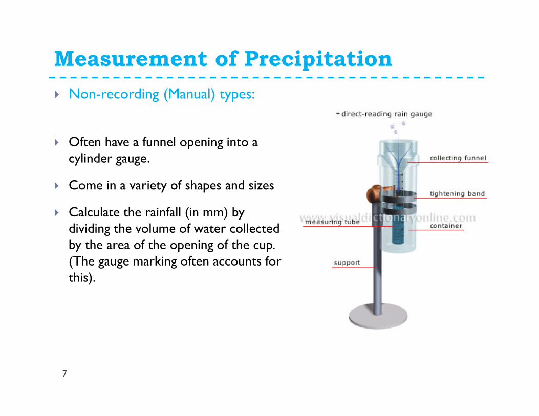
� Non-recording (Manual) types:
� Often have a funnel opening into a cylinder gauge.
� Come in a variety of shapes and sizes
� Calculate the rainfall (in mm) by dividing the volume of water collected by the area of the opening of the cup. (The gauge marking often accounts for this).

Measurement of Precipitation
8
� Non-recording (Manual) types:
Measurement of Precipitation
9
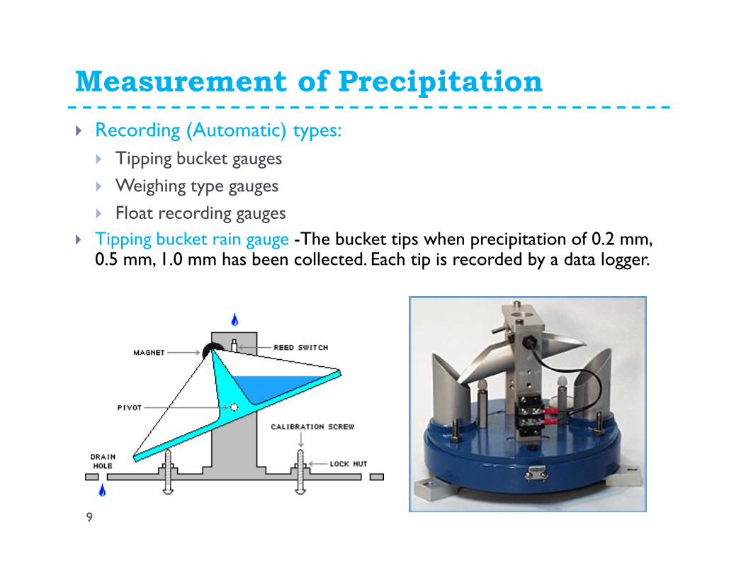
� Recording (Automatic) types:
� Tipping bucket gauges
� Weighing type gauges
� Float recording gauges
� Tipping bucket rain gauge -The bucket tips when precipitation of 0.2 mm, 0.5 mm, 1.0 mm has been collected. Each tip is recorded by a data logger.

Measurement of Precipitation
10
� Recording (Automatic) types:
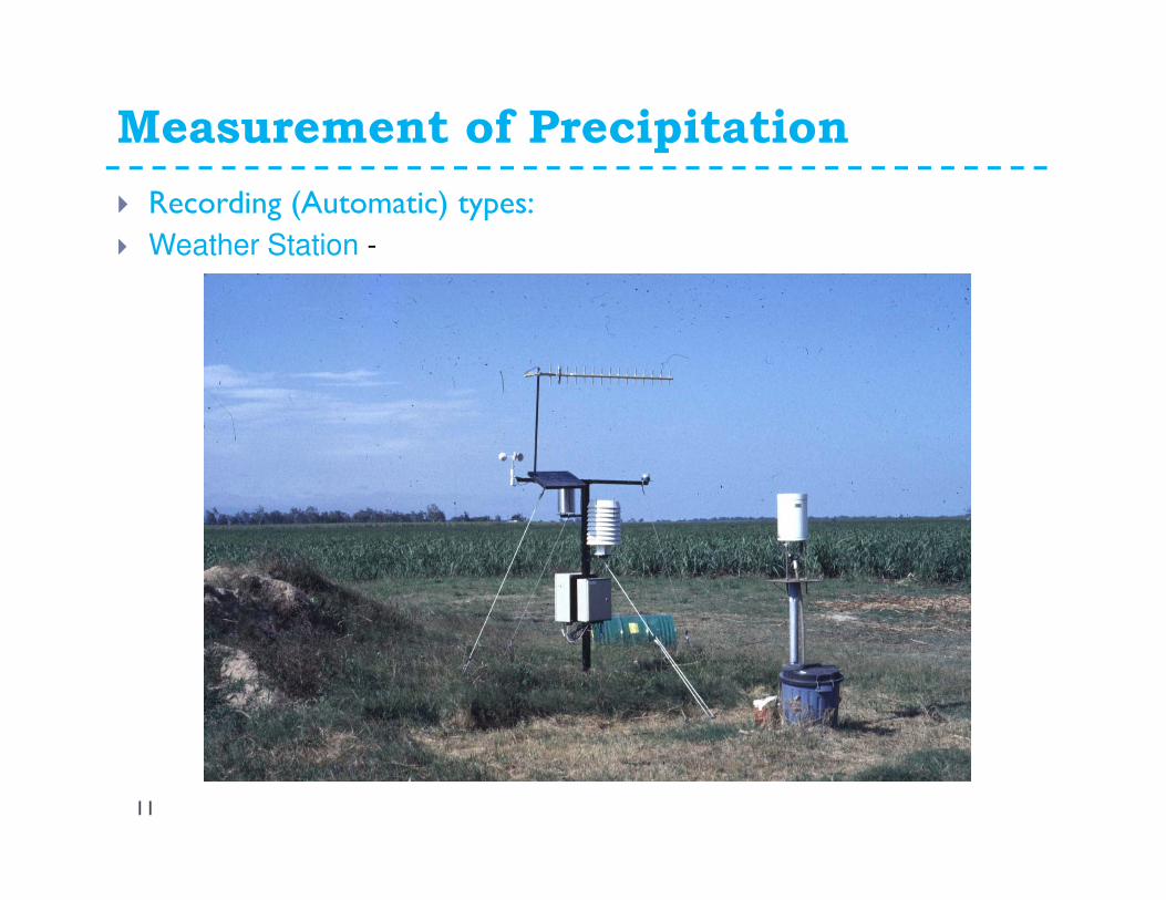
� Weather Station - Records rainfall, but also evaporation, air pressure, air temperature, wind speed and wind direction (so can be used to estimate evapo-transpiration)
� Radar - Ground-based radar equipment can be used to determine
how much rain is falling and where it is the heaviest.
Measurement of Precipitation
11
� Recording (Automatic) types:
� Weather Station -

Measurement of Precipitation
12
� Recording (Automatic) types:
� Radar -

Measurement of Precipitation
Raingauge Network
13
� Since the catching area of the raingauge is very small as compared tothe areal extent of the storm, to get representative picture of astorm over a catchment the number of raingauges should be aslarge as possible, i.e. the catchment area per gauge should be small.
� There are several factors to be considered to restrict the number ofgauges:
� Like economic considerations to a large extent
� Topographic & accessibility to some extent.
Catchment area: An extent of land where water from precipitation drains into a body of water

Measurement of Precipitation
Raingauge Network
14
� World Meteorological Organization (WMO) recommendation:
� In flat regions of temperate,Mediterranean and tropical zones
� Ideal� 1 station for 600 – 900 km2
� Acceptable�1 station for 900 – 3000 km2
� In mountainous regions of temperate , Mediterranean and tropical zones
� Ideal� 1 station for 100 – 250 km2
� Acceptable� 1 station for 250 – 1000 km2
� In arid and polar zone
� 1 station for 1500 – 10,000 km2
� 10 % of the raingauges should be self recording to know the intensity ofthe rainfall !!

Measurement of Precipitation
Raingauge Network
15
� Placement of rainguages
� Gauges are affected by wind pattern, eddies, trees and the
gauge itself, therefore it is important to have the gauge located
and positioned properly.
� Raingauges should be
� 1m above ground level is standard -
� All gauges in a catchment should be the same height
� 2 to 4 times the distance away from an isolated object (such as a tree or building) or in a forest a clearing with the radius at least the tree height or place the gauge at canopy level
� shielded to protect gauge in windy sites or if obstructions are numerous they will reduce the wind-speed, turbulence and eddies.

Measurement of Precipitation
Raingauge Network
16
Rainguage with wind shield

Measurement of Precipitation
Raingauge Network
17
• For sloping ground the gauge should be placed with the opening parallel to the ground
• The rainfall catch volume (mm3) is then divided by the opening area that the rain can enter

Measurement of Precipitation
Sources of Errors
18
� Instrument error� Observer error� Errors due to different observation times� Error due to occult precipitation� Errors due to low-intensity rains
� Any-other ?
� _________________________________
Occult precipitation: Precipitation arriving at a location by processes that would normally go unrecorded by a standard rain gauge, e.g. the condensation of mist and fog on foliage.

Preparation of Data
19
� Before using rainfall data for any analysis, it is necessary to check the record for
� Missing data and/or
� Consistency of data
� Inconsistency in rainfall data my root from
� Change of gauge location� Change of gauge type� Change of gauge environment� Change of gauge observer� Change of gauge climate

Preparation of Data: Missing Data
Methods
� The following methods can be used to estimate the missing precipitation data
� Station-average method
� Normal-ratio method
� Inverse-distance weighting
� Regression
20

21
PX is the missing precipitation value for station X P1, P2, …, Pn are precipitation values at the adjacent stations for the same period n is the number of nearby stations
Preparation of Data: Missing Data
Station Average Method
PX =1
nPi
i=1
n
∑
This method is used when 10% variation in annual precipitation at station X lies within annual precipitation of surrounding/adjacent stations.

22
� Find out the missing storm precipitation data of station X given in following table using station averaging method
Preparation of Data: Missing Data
Example
Station 1 2 X 3 4
Storm Precipitation (inches) 3.8 3.25 ? 4.6 3.15
Annual Precipitation (inches) 39.50 43.1 36.8 49.5 46.20
What about 10% variation check from annual precipitation ??
( ) inPn
Pn
i
iX 7.315.36.425.38.34
11
1
=+++== ∑=

23
Preparation of Data: Missing Data
Normal Ratio Method
� PX is the missing precipitation value for station X for a certain time period
� P1, P2, …, Pn are precipitation values at adjacent stations for the same period
� NX is the long-term, annual average precipitation at station X
� N1, N2, …, Nn is the long-term precipitation for neighboring stations
� n is the number of adjacent stations
PX
NX
=1
n
P1
N1
+P2
N2
+ ..... +Pn
Nn
PX =
1
n
Pi
Nii=1
n
∑ NXor

24
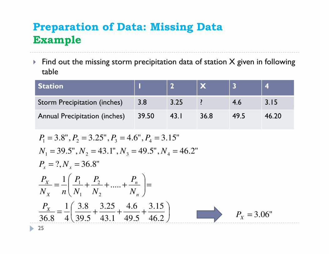
� Find out the missing storm precipitation data of station X given in following table
Preparation of Data: Missing Data
Example
Station 1 2 X 3 4
Storm Precipitation (inches) 3.8 3.25 ? 4.6 3.15
Annual Precipitation (inches) 39.50 43.1 36.8 49.5 46.20
Test the normal annual precipitation at station X
inandin
inof
12.3348.408.3668.3
68.38.36%10
=+±
=
Since annual precipitation of adjacent station does not lie with 10% so station averaging method cannot be used and instead normal ratio method will be used for better accuracy
25
� Find out the missing storm precipitation data of station X given in following table
Preparation of Data: Missing Data
Example
Station 1 2 X 3 4
Storm Precipitation (inches) 3.8 3.25 ? 4.6 3.15
Annual Precipitation (inches) 39.50 43.1 36.8 49.5 46.20
+++=
=
+++=
==
====
====
2.46
15.3
5.49
6.4
1.43
25.3
5.39
8.3
4
1
8.36
.....1
"8.36?,
"2.46,"5.49,"1.43,"5.39
"15.3,"6.4,"25.3,"8.3
2
2
1
1
4321
4321
X
n
n
X
X
xx
P
N
P
N
P
N
P
nN
P
NP
NNNN
PPPP
"06.3=XP

26
� Example
Preparation of Data: Missing Data
Station Average Method

27
1. di = (xi2 + yi
2)0.5
� PX is the missing precipitation value for station X for a certain time period
� Pi are precipitation values at adjacent stations for the same period
� n is the number of neighboring stations
PX =1
Wdi
−bPi
i=1
n
∑3.
W = di−b
i=1
n
∑2.
• Distance from gage with missing data to the neighboring gages
• Weight of distances where b is a proportionality factor (b = 1, 2 )
Preparation of Data: Missing Data
Inverse Distance Weighing

Preparation of Data: Missing Data
Regression
� PX is the missing precipitation value for station X for certain time period
� P1, P2, …, Pn are precipitation values at the neighboring stations for the same period
� b0, …, bn are coefficients calculated by least-squares methods
� n is the number of nearby gages
� This method is suitable when there is a large number of days when observations are available for all gages
PX = bo + b1P1 + b2P2 + …. + bnPn
28

• Let’s take a group of 5 to 10 base stations in the neighbourhood of the problem station X is selected
• Arrange the data of stn X rainfall and the average of the neighbouringstations in reverse chronological order (from recent to old record)
• Accumulate the precipitation of station X and the average values of the group base stations starting from the latest record.
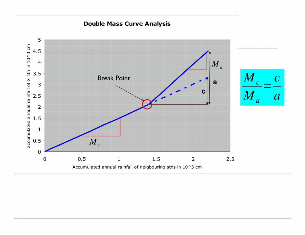
• Plot the against as shown on the next figure
• A decided break in the slope of the resulting plot is observed that indicates a change in precipitation regime of station X, i.e., inconsistency.
• Therefore, data at stn X should be corrected/adjusted as
Pcx=(Mc/Ma)*Px
Mc is slope of data before breakpoint
Ma is slope of line after breakpoint
Pcx is corrected precipitation at StationX
Px is original precipitation at StationX
( )∑ xP
( )∑ avgP( )∑ xP
( )∑ avgP
Preparation of Data: Consistency of Data
Double Mass Curve Technique
29
a
c
xcxM
MPP =
Pcx – corrected precipitation at any time period t1 at stationX
Px – Original recorded precp. at time period t1 at station X
Mc – corrected slope of the double mass curve
Ma – original slope of the mass curve after break
Double Mass Curve Analysis
0
0.5
1
1.5
2
2.5
3
3.5
4
4.5
5
0 0.5 1 1.5 2 2.5
Accumulated annual rainfall of neigbouring stns in 10^3 cm
accumulated annual rainfall of X stn in 10^3 cm
c
a
a
c
M
M
a
c =
30
cM
aM
Break Point

Preparation of Data: Consistency of Data
Double Mass Curve Technique
31
(i). Check whether the data of station X is consistent(ii). In which year change indicated?(iii). Compute the mean annual rainfall for station X at its present site for the given 36 year period first without adjustment and secondly with the data adjusted for the change in regime.(iv). Compute the adjusted annual rainfall at station X for the affected period.

32
Preparation of Data: Consistency of Data
Double Mass Curve Technique

33
Preparation of Data: Consistency of Data
Double Mass Curve Technique

34
Preparation of Data: Consistency of Data
Double Mass Curve Technique

Part II
35

Temporal and Spatial Variation of Rainfall
� Rainfall varies greatly both in time and space
� With respect to time –Temporal variation
� With space – Spatial variation
� The temporal variation may be defined as hourly, daily, monthly, seasonalvariations and annual variation (long-term variation of precipitation)
Temporal Variation of rainfall at a particular site
Total Rainfall amount = 6.17 cm
0
2
4
6
8
10
12
14
0 20 40 60 80 100 120 140
Time, min
Rainfall Intensity, cm/hr
36

Temporal and Spatial Variation of Rainfall
37
Long term Precipitation variation at Arba Minch
0
5
10
15
20
25
30
35
40
45
1986 1988 1990 1992 1994 1996 1998 2000 2002 2004 2006
Years
Annual ra
infa
ll, m
m
Annual Precipitation
average precipitation

Temporal and Spatial Variation of Rainfall
38
� Source: Gary R Fuelner, Rainfall and climate records from Sharjah Airport: Historical data for the study of recent climatic periodicity in the U.A.E.

Temporal Averaging of Precipitation
39
� Storm rainfall/precipitation: It is the precipitation of a particular storm/rainfall event.
� Daily Rainfall: The amount of rainfall accumulated in one day at a place, Mathematically;
� Where Pday is daily rainfall and Pi is hourly storm rainfall during a given day.
� Monthly Rainfall: The amount of rainfall accumulated in one month at a place, Mathematically;
� Where Pmonth is monthly rainfall and Pday is daily precipitation during a given month.
∑=
=24
1i
iday PP
∑=
=30
dayi
daymonth PP

Temporal Averaging of Precipitation
40
� Annual Rainfall: The amount of rainfall accumulated in one year at a place, Mathematically;
� Where Pann is annual rainfall and Pday is daily rainfall
� Average rainfall for N years: It is the arithmetic average of annual precipitation for N years over a rain gauging station. Mathematically;
� Where Pavg is average rainfall for N years and Pi is annual rainfall for ith
year
N
P
P
N
i
i
avg
∑== 1
∑=
=365
dayi
dayann PP

Temporal Averaging of Precipitation
41
� Estimate average monthly and annual precipitation from given data
∑=
=365
1i
ann PiP ∑=
=12
1i
ann PiP
( ) 3.942.167.21.1008.004.02.71.22258.18 =+++++++++++=annP
Average Monthly Precipitation ?
Annual Precipitation ?
( ) mmN
Pi
P
N
iavg 86.712/2.167.21.1008.004.02.71.22258.181 =+++++++++++==
∑=

42
Climate data for DubaiMonth Jan Feb Mar Apr May Jun Jul Aug Sep Oct Nov Dec Year
Record high °C (°F)
31.6(88.9)
37.5(99.5)
41.3(106.3)
43.5(110.3)
47.0(116.6)
46.7(116.1)
49.0(120.2)
48.7(119.7)
45.1(113.2)
42.0(107.6)
41.0(105.8)
35.5(95.9)
49(120.2)
Average high °C (°F)
24.0(75.2)
25.4(77.7)
28.2(82.8)
32.9(91.2)
37.6(99.7)
39.5(103.1)
40.8(105.4)
41.3(106.3)
38.9(102)
35.4(95.7)
30.5(86.9)
26.2(79.2)
33.4(92.1)
Daily mean °C (°F)
19(66)
20(68)
22.5(72.5)
26(79)
30.5(86.9)
33(91)
34.5(94.1)
35.5(95.9)
32.5(90.5)
29(84)
24.5(76.1)
21(70)
27.5(81.5)
Average low °C (°F)
14.3(57.7)
15.4(59.7)
17.6(63.7)
20.8(69.4)
24.6(76.3)
27.2(81)
29.9(85.8)
30.2(86.4)
27.5(81.5)
23.9(75)
19.9(67.8)
16.3(61.3)
22.3(72.1)
Record low °C (°F)
6.1(43)
6.9(44.4)
9.0(48.2)
13.4(56.1)
15.1(59.2)
18.2(64.8)
20.4(68.7)
23.1(73.6)
16.5(61.7)
15.0(59)
11.8(53.2)
8.2(46.8)
6.1(43)
Precipitation mm (inches)
18.8(0.74)
25.0(0.984)
22.1(0.87)
7.2(0.283)
0.4(0.016)
0.0(0)
0.8(0.031)
0.0(0)
0.0(0)
1.1(0.043)
2.7(0.106)
16.2(0.638)
94.3(3.711)
Avg. precipitation days
5.4 4.7 5.8 2.6 0.3 0.0 0.5 0.5 0.1 0.2 1.3 3.8 25.2
% humidity 65 65 63 55 53 58 56 57 60 60 61 64 59.8
Mean monthly sunshine hours
254.2 229.6 254.5 294.0 344.1 342.0 322.4 316.2 309.0 303.8 285.0 256.6 3,511.4
Source #1: Dubai Meteorological Office[4]
Source #2: climatebase.ru (extremes, sun),[5], NOAA (humidity, 1974-1991)[6]42

Spatial Averaging of Precipitation
43
� Average rainfall over an area: It is the amount of precipitation which can be assumed as uniform over the given area.
� It is estimated by using several approaches given below;� Arithmetic method
� Theissen polygon method
� Isohyetal method
� According to arithmetic method, arithmetic mean precipitation over an area can be defined by
� Where, Pavg is the average precipitation, N is the total number of stations and Pi is the average annual precipitation for ith station.
N
Pi
P
N
iavg
∑== 1

Methods of Spatial Averaging Rainfall Data
44
� Raingauges rainfall represent only point sampling of the areal distribution of a storm
� The important rainfall for hydrological analysis is a rainfall over an area, such as over the catchment
� To convert the point rainfall values at various stations in to average value over a catchment, the following methods are used:
� (i). arithmetic mean method
� (ii). the method of the Thiessen polygons
� (iii). the isohyetal method

• When the area is physically and climatically
homogenous and the required accuracy is small,
the average rainfall ( ) for a basin can be
obtained as the arithmetic mean of the Pi values
recorded at various stations.
• Applicable rarely for practical purpose
∑=
=++++
=N
i
i
ni PNN
PPPPP
1
21 1..........
P
Methods of Spatial Averaging Rainfall Data
Arithmetic Mean Method
45

• The method of Thiessen polygons consists of attributing to
each station an influence zone in which it is considered that
the rainfall is equivalent to that of the station.
• The influence zones are represented by convex polygons.
• These polygons are obtained using the mediators of the
segments which link each station to the closest
neighbouring stations
Methods of Spatial Averaging Rainfall Data
Thiessen Polygon Method
46

Methods of Spatial Averaging Rainfall Data
Thiessen Polygon Method
47

A1
A2
A3A4
A5
A6
A7
A8P1
P2
P3
P4
P5
P6
P7
P8
Methods of Spatial Averaging Rainfall Data
Thiessen Polygon Method
48

( )m
mm
AAA
APAPAPP
+++
+++=
.....
.....
21
2211
∑∑
=
= ==M
i
ii
total
i
M
i
i
A
AP
A
AP
P1
1
Generally for M station
The ratio is called the weightage factor of station iA
Ai
Methods of Spatial Averaging Rainfall Data
Thiessen Polygon Method
49

50
Methods of Spatial Averaging Rainfall Data
Thiessen Polygon Method

51Mean precipitation = =121.84
Methods of Spatial Averaging Rainfall Data
Thiessen Polygon Method
A
AiiP
A
AP i
i=
∑=
M
i
ii
A
AP
1
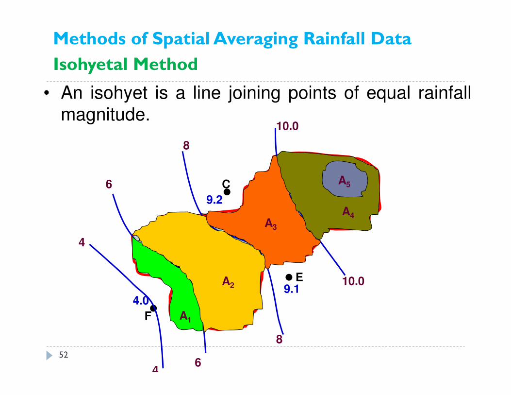
• An isohyet is a line joining points of equal rainfall
magnitude.
F
B
EA
CD
129.2
4.0
7.0
7.2
9.110.0
10.0
12
8
8
6
6
4
4
A1
A2
A3
A4
A5
Methods of Spatial Averaging Rainfall Data
Isohyetal Method
52

• P1, P2, P3, …. , Pn – the values of the isohytes
• A1, A2, A3, …., A4 – are the inter isohytes area respectively
• Atotal – the total catchment area
• - the mean precipitation over the catchmentP
total
nnn
A
PPA
PPA
PPA
P
+++
++
+
=
−−
2...
22
11
322
211
The isohyet method is superior to the other two methods especially when the stations are large in number.
NOTE
Methods of Spatial Averaging Rainfall Data
Isohyetal Method
53

54
Methods of Spatial Averaging Rainfall Data
Isohyetal Method

55
2
1++
= iiavg
PPP
total
i
A
AiA
total
iavg
A
AP

� Other mapping programs such as SURFER or GIS program ARCVIEW can be used to map rainfall at the different measurement locations.
56
Methods of Spatial Averaging Rainfall Data
Isohyetal Method
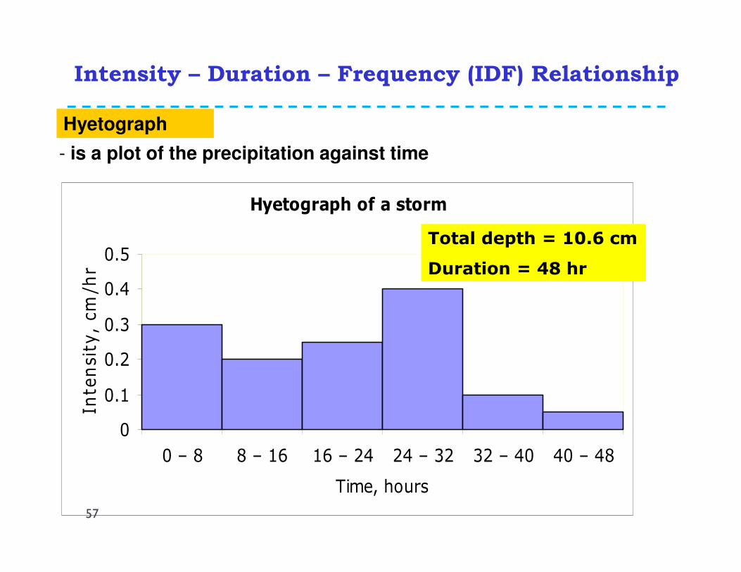
Hyetograph
- is a plot of the precipitation against time
Hyetograph of a storm
0
0.1
0.2
0.3
0.4
0.5
0 – 8 8 – 16 16 – 24 24 – 32 32 – 40 40 – 48
Time, hours
Intensity, cm/hr
Total depth = 10.6 cm
Duration = 48 hr
57
Intensity – Duration – Frequency (IDF) Relationship
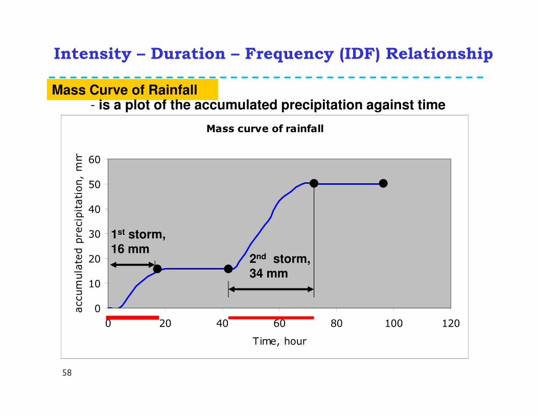
Mass Curve of Rainfall
Mass curve of rainfall
0
10
20
30
40
50
60
0 20 40 60 80 100 120
Time, hour
accumulated precipitation, mm
1st storm,
16 mm 2nd storm, 34 mm
- is a plot of the accumulated precipitation against time
58
Intensity – Duration – Frequency (IDF) Relationship

Intensity – Duration – Frequency (IDF)
Relationship
59
� Example: The mass curve of rainfall in a storm of total duration 270 minutes is given below. Draw the hyetograph of the storm at 30 minute time step.
0
5
10
15
20
25
30
35
30 60 90 120 150 180 210 240 270
Rainfall intensity (mm/hr)
Time (min)
Hyetograph
Time since start (min) 0 30 60 90 120 150 180 210 240 270
Cumulative Rainfall (mm) 0 6 18 21 36 43 49 52 53 54
Incremental depth in interval of 30 min (mm) 6 12 3 15 7 6 3 1 1
Rainfall intensity (mm/hr) 12 24 6 30 14 12 6 2 2

Intensity – Duration – Frequency (IDF)
Relationship
60
� Return Period (T) - The average length of time in years for an event (e.g. flood or rainfall) of given magnitude to be equalled or exceeded.
� For example, if the rainfall with a 50 year return period at a given location is 200mm, this is just another way of saying that a rainfall 200mm, or greater, should occur at that location on the average only once every 50 years.
� Probability of Occurrence (p) (of an event of specified magnitude) -The probability that an event of the specified magnitude will be equalled or exceeded during a one year period.
� Basic Relationships
T=1/P or P=1/T
Intensity – Duration – Frequency (IDF)
Relationship
61
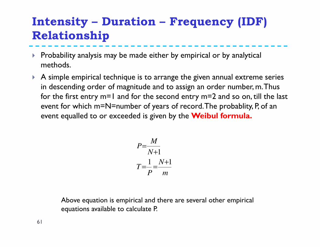
� Probability analysis may be made either by empirical or by analytical methods.
� A simple empirical technique is to arrange the given annual extreme series in descending order of magnitude and to assign an order number, m. Thus for the first entry m=1 and for the second entry m=2 and so on, till the last event for which m=N=number of years of record. The probablity, P, of an event equalled to or exceeded is given by the Weibul formula.
m
N
PT
N
MP
11
1
+==
+=
Above equation is empirical and there are several other empirical equations available to calculate P.

Intensity – Duration – Frequency (IDF)
Relationship
62
� The record of annual rainfall at station A covering a period of 22 years is given below.
� (a). Estimate the annual rainfall with return periods of 10 years and 23 years (b). What would be the probability of an annual rainfall of magnitude equal to or exceeding 100cm.
YearAnnual Rainfall
(cm) YearAnnual Rainfall
(cm)
1960 130 1971 90
1961 84 1972 102
1962 76 1973 108
1963 89 1974 60
1964 112 1975 75
1965 96 1976 120
1966 80 1977 160
1967 125 1978 85
1968 143 1979 106
1969 89 1980 83
1970 78 1981 95

mAnnual
Rainfall (cm)Probability P=m/(N+1)
Return Period T (years)
1 160 0.043 23.00
2 140 0.087 11.50
3 130 0.130 7.67
4 125 0.174 5.75
5 120 0.217 4.60
6 112 0.261 3.83
7 108 0.304 3.29
8 106 0.348 2.88
9 102 0.391 2.56
10 96 0.435 2.30
11 95 0.478 2.09
12 90 0.522 1.92
13 89 0.565 1.77
14 89 0.609 1.64
15 85 0.652 1.53
16 84 0.696 1.44
17 83 0.739 1.35
18 80 0.783 1.28
19 78 0.826 1.21
20 76 0.870 1.15
21 75 0.913 1.10
22(=N) 60 0.957 1.05
(a). Annual rainfall for 10 years return period. By interpolation, P=137.5cmAnnual rainfall for 23 years return period. P=160cmAnnual rainfall for 50 years return period. By extrapolation, P= ??cm
(b). Return period of P=100cm is 2.4 (by interpolation between 102 and 96)

� In many design problems related to watershed such as runoffdisposal, erosion control, highway construction, culvert design, itis necessary to know the rainfall intensities of different durationsand different return periods.
� The curve that shows the inter-dependency between i (cm/hr), D(hour) andT (year) is called IDF curve.
� The relation can be expressed in general form as:
( )n
x
aD
Tki
+=
i – Intensity (cm/hr)
D – Duration (hours)
K, x, a, n – are constant for a given catchment
Intensity – Duration – Frequency (IDF) Relationship
64
IDF Curve

Typical IDF Curve
0
2
4
6
8
10
12
14
0 1 2 3 4 5 6
Duration, hr
Intesity, cm/hr
T = 25 years
T = 50 years
T = 100 years
k = 6.93
x = 0.189
a = 0.5
n = 0.878
Intensity – Duration – Frequency (IDF) Relationship
65

Thank you
� Questions….
66


