Precipitation-Runoff Processes in the Feather River Basin, Northeastern California, with Prospects for Streamflow Predictability, Water Years 1971–97 By Kathryn M. Koczot, Anne E. Jeton, Bruce J. McGurk, and Michael D. Dettinger In cooperation with the California Department of Water Resources Scientific Investigations Report 2004-5202 U.S. Department of the Interior U.S. Geological Survey
Transcript
Precipitation-Runoff Processes in the Feather River Basin, Northeastern California, with Prospects for Streamflow Predictability, Water Years 1971–97
By Kathryn M. Koczot, Anne E. Jeton, Bruce J. McGurk, and Michael D. Dettinger
In cooperation with the California Department of Water Resources
Scientific Investigations Report 2004-5202
U.S. Department of the Interior U.S. Geological Survey
U.S. Geological Survey, Reston, Virginia: 2005For sale by U.S. Geological Survey, Information Services Box 25286, Denver Federal Center Denver, CO 80225-0286
U.S. Department of the InteriorGale A. Norton, Secretary
U.S. Geological SurveyCharles G. Groat, Director
For more information about the USGS and its products: Telephone: 1-888-ASK-USGS World Wide Web: http://www.usgs.gov/
Any use of trade, product, or firm names in this publication is for descriptive purposes only and does not imply endorsement by the U.S. Government.
Although this report is in the public domain, permission must be secured from the individual copyright owners to reproduce any copyrighted materials contained within this report.
Suggested citation: Koczot, K.M., Jeton, A.E., McGurk, B.J., and Dettinger., M.D., 2005, Precipitation-runoff processes in the Feather River Basin, northeastern California, with prospects for streamflow predictability, water years 1971–97: U.S. Geological Survey Scientific Investigations Report 2004–5202, 82 p.
Figure 1. Map showing Feather River Basin, California, modeled areas, major tributaries and reservoirs, larger towns, county lines, selected peaks and valleys, and stations where streamflow or climate variables used in the models are measured or reconstructed . . . . . . . . . . . . . . . . . . . . . . . . . . 3
Figure 2. Schematic diagram of Feather River, California, showing Oroville Complex water-supply and hydropower facilities (including Lake Oroville), other improvements downstream from Lake Oroville including diversions for irrigation, and the locations of the U.S. Geological Survey streamflow stations from which monthly estimates of inflow to Lake Oroville are derived. . . . . . . . . . . . . . . . . . . . . . . . . . . . . . . . . . . . . . . . . . . . . . . . . . 5
Figure 3. Map and graph showing altitudes above and below the snow line and area at altitudes in the Feather River Basin, California . . . . . . . . . . . . . . . . . . . . . . . . . . . . . . . 7
Figure 4. Schematic diagrams showing North Fork and South Fork Feather River powerhouses and locations of reconstructed streamflow, Feather River Basin, California . . . . . . . . . . . . . . . . . . . . . . . . . . . . . . . . . . . . . . . . . . . . . . . . . . . . . . . . . 10
Figure 6. Maps showing geology and soil texture of the Feather River Basin, California. . . . . . . 12Figure 7. Map showing modeled areas and supporting catchments, and streamflow
and climate stations, in/near the Feather River Basin, California . . . . . . . . . . . . . . . 13Figure 8. Maps showing distributions of precipitation over the Feather River Basin,
California, including 30-year mean-annual, and selected 30-year mean-monthly, November, January, May, and September patterns. . . . . . . . . . . . . 19
Figure 9. Graphs showing mean-monthly precipitation for the Feather River Basin measured at climate stations during the modeling period 1971–97, measured in the 1961–90 period, and estimated from Precipitation-Elevation Regressions on Independent Slopes Model at locations of the precipitation stations for 1961–90. . . . . . . . . . . . . . . . . . . . . . . . . . 21
Figure 10. Graph showing minimum correlation of precipitation measurements between stations used in watershed modeling of the Feather River Basin, California, water years 1971–97 . . . . . . . . . . . . . . . . . . . . . . . . . . . . . . . . . . . . . . . . . . . . 22
Figure 13. Diagrams showing Precipitation-Runoff Modeling System conceptually illustrated, including schematic diagram of the conceptual water system and inputs, and components of the snowpack energy-balance equations . . . . . . . 31
Figure 14. Map showing hydrologic response units and model areas delineated for the Feather River Basin Precipitation-Runoff Modeling System, California. . . . . . . 41
Figure 15. Diagrams showing draper method to estimate daily precipitation from Parameter-Elevation Regressions on Independent Slopes Model (PRISM) surfaces, including observed daily precipitation as a percent of normal at each observation site, an example of a mean-monthly PRISM precipitation surface, and resulting draped precipitation estimates . . . . . . . . . . . . . . . . . . . . . . . . 43
Figure 16. Graphs showing daily streamflow hydrographs showing model simulations and observed (measured or reconstructed) streamflow, water years 1971–97, including Almanor, Butt Creek, Lower North Fork, East Branch, Middle Fork, West Branch, South Fork, and Oroville . . . . . . . . . . . . . . . . . . . . . . . . . . . . . . . . . 46
Figure 18. Graph showing mean-monthly percentages of simulated inflows to Lake Oroville and the Feather River at Oroville reconstructed streamflow, water years 1971–97. . . . . . . . . . . . . . . . . . . . . . . . . . . . . . . . . . . . . . . . . . . . . . . . . . . . . . 49
Figure 19. Graphs showing seasonal streamflow into Lake Oroville in water years 1971–97, including January–March, and April–July. . . . . . . . . . . . . . . . . . . . . . . . . . . 51
Figure 20. Graph showing total annual inflow to Lake Oroville, water years 1971–2000. . . . . . . . 52Figure 21. Map showing simulated and remotely sensed snow cover for the
Table 3. Correlation of precipitation (water-year means) between stations used in watershed modeling of the Feather River Basin, California, water years 1971–97 . . . . . . . . . . . . . . . . . . . . . . . . . . . . . . . . . . . . . . . . . . . . . . . . . . . . . . . . . . . . . . . . . 23
Table 4. Period-of-record percentages of days with maximum (first number) and minimum (second number) temperatures less than or equal to freezing at climate stations in the Feather River Basin, California . . . . . . . . . . . . . . . . . . . . . . 24
Table 5. Period-of-record percentages of days with observed precipitation with maximum (first number) and minimum (second number) temperatures less than or equal to freezing at climate stations in the Feather River Basin, California . . . . . . . . . . . . . . . . . . . . . . . . . . . . . . . . . . . . . . . . . . . . . . . . . . . . . . . . . . . . . . . 24
Table 10. Mean-monthly reconstructed (R) or measured (M) streamflow for areas modeled as percent of annual total, water years 1971–97, and Lake Oroville (FTO) 1906–2000; peak monthly streamflow listed in bold. . . . . . . . . . . . . . . 29
Table 12. Source of parameter values for selected Hydrologic Response Unit [HRU] (distributed) and whole-model (non-distributed) Precipitation-Runoff Modeling System (PRMS) parameters for the Feather River Basin, California (modified from Jeton, 1999b) . . . . . . . . . . . . . . . . . . . . . . . . . . . . . . . . . . . . . 37
Table 13. Model Hydrologic Response Unit (HRU) counts and ranges within each model of specified-HRU areas, mean altitudes, mean slopes, and mean aspects . . . . . . . . . . . . . . . . . . . . . . . . . . . . . . . . . . . . . . . . . . . . . . . . . . . . . . . . . . . . . . . . . 40
Table 14. Calibration statistics, Feather River Basin, California, water years 1971–97 . . . . . . . . . 45Table 15. Percentages of annual inflow to Lake Oroville from modeled areas:
simulated, and measured or reconstructed. . . . . . . . . . . . . . . . . . . . . . . . . . . . . . . . . . 58Table 16. Average-annual simulated components of streamflow in the Feather River
Table 17. Average-annual simulated water-budget analysis in the Feather River Basin, water years 1971–97, with measured or reconstructed streamflow . . . . . . . 60
vii
Appendixes
Appendix A. Components of reconstructed natural streamflow of the Feather River at Oroville, California (FTO), computed as acre-feet per month. . . . . . . . . . . . 70
Appendix B. Programming for the draper method to estimate precipitation over Hydrologic Response Unit (HRU) surfaces from PRISM simulations, Feather River Basin, California. . . . . . . . . . . . . . . . . . . . . . . . . . . . . . . . . . . . . . . . . . . . . 71
Appendix C. Name, size, and description of data and parameter files used for the Feather River PRMS models . . . . . . . . . . . . . . . . . . . . . . . . . . . . . . . . . . . . . . . . . . . . . . . 82
viii
Conversion Factors, Datum, Abbreviations, and Acronyms
CONVERSION FACTORS
Temperature in degrees Fahrenheit (oF) may be converted to degrees Celsius (oC) as follows:oC=(oF-32)/1.8.
DATUM
Vertical coordinate information is referenced to National Geodetic Vertical Datum of 1929 (NGVD 29). Horizontal coordinate information is referenced to the North American Datum of 1927 (NAD 27).
Altitude, as used in this report, refers to distance above the vertical datum.
Water Year constitutes a 12-month period from October 1 through September 30, and is desig-nated by the year in which the period ends (for example, water year 1995 began October 1, 1994, and ended September 30, 1995).
ABBREVIATIONS
asl above sea level
ACRONYMS
ESP Ensemble Streamflow Prediction
FTO Feather River at Oroville
GIS geographic information system
HRU hydrologic response unit
MMS Modular Modeling System
NWSRFS National Weather Service River Forecasting System
PDO Pacific Decadal Oscillation
PRISM Parameter-Elevation Regressions on Independent Slopes Model
PRMS Precipitation-Runoff Modeling System
Multiply By To obtainacre 4,047 square meter
acre-feet (acre-ft) 1,233 cubic metercubic foot per second (ft3/s) 0.02832 cubic meter per second
foot (ft) 0.3048 meterinch (in.) 2.54 centimeter
inch per year (in/yr) 2.54 centimeter per yearmile (mi) 1.609 kilometer
square mile (mi2) 12.590 square kilometer
ix
RMSE root-mean-square error
SCCT Snow Cover Comparison Tool
Organizations
CCSS California Cooperative Snow Surveys Program
CDEC California Data Exchange Center
CNRFC National Oceanic and Atmospheric Administration’s California-Nevada
River Forecasting Center
DWR California Department of Water Resources
HEC U.S. Army Corps of Engineers Hydrologic Engineering Center
NASA National Aeronautics and Space Administration
NOAA National Oceanic and Atmospheric Administration
NOHRSC National Operational Hydrologic Remote Sensing Center
PG&E Pacific Gas & Electric Company
SWP California State Water Project
USDA U.S. Department of Agriculture
USFS U.S. Forest Service
USGS U.S. Geological Survey
x
Precipitation-Runoff Processes in the Feather River Basin, Northeastern California, and Streamflow Predictability, Water Years 1971–97
By Kathryn M. Koczot1, Anne E. Jeton1, Bruce J. McGurk2, and Michael D. Dettinger1
Abstract
Precipitation-runoff processes in the Feather River Basin of northern California determine short- and long-term streamflow variations that are of considerable local, State, and Federal concern. The river is an important source of water and power for the region. The basin forms the headwaters of the California State Water Project. Lake Oroville, at the outlet of the basin, plays an important role in flood management, water quality, and the health of fisheries as far downstream as the Sacramento-San Joaquin Delta. Existing models of the river simulate streamflow in hourly, daily, weekly, and seasonal time steps, but cannot adequately describe responses to climate and land-use variations in the basin. New spatially detailed precipitation-runoff models of the basin have been developed to simulate responses to climate and land-use variations at a higher spatial resolution than was available previously. This report characterizes daily rainfall, snowpack evolution, runoff, water and energy balances, and streamflow variations from, and within, the basin above Lake Oroville. The new model’s ability to predict streamflow is assessed.
The Feather River Basin sits astride geologic, topographic, and climatic divides that establish a hydrologic character that is relatively unusual among the basins of the Sierra Nevada. It straddles a north-south geologic transition in the Sierra Nevada between the granitic bedrock that underlies and forms most of the central and southern Sierra Nevada and volcanic bedrock that underlies the northernmost parts of the range (and basin). Because volcanic bedrock generally is more permeable than granitic, the northern, volcanic parts of the basin contribute larger fractions of ground-water flow to streams than do the southern, granitic parts of the basin. The
Sierra Nevada topographic divide forms a high altitude ridgeline running northwest to southeast through the middle of the basin. The topography east of this ridgeline is more like the rain-shadowed basins of the northeastern Sierra Nevada than the uplands of most western Sierra Nevada river basins. The climate is mediterranean, with most of the annual precipitation occurring in winter. Because the basin includes large areas that are near the average snowline, rainfall and rain-snow mixtures are common during winter storms. Consequently, the overall timing and rates of runoff from the basin are highly sensitive to winter temperature fluctuations.
The models were developed to simulate runoff-generating processes in eight drainages of the Feather River Basin. Together, these models simulate streamflow from 98 percent of the basin above Lake Oroville. The models simulate daily water and heat balances, snowpack evolution and snowmelt, evaporation and transpiration, subsurface water storage and outflows, and streamflow to key streamflow gage sites. The drainages are modeled as 324 hydrologic-response units, each of which is assumed homogeneous in physical characteristics and response to precipitation and runoff. The models were calibrated with emphasis on reproducing monthly streamflow rates, and model simulations were compared to the total natural inflows into Lake Oroville as reconstructed by the California Department of Water Resources for April–July snowmelt seasons from 1971 to 1997. The models are most sensitive to input values and patterns of precipitation and soil characteristics. The input precipitation values were allowed to vary on a daily basis to reflect available observations by making daily transformations to an existing map of long-term mean monthly precipitation rates that account for altitude and rain-shadow effects.
1U.S. Geological Survey
2Pacific Gas & Electric Company
2 Precipitation-Runoff Processes in the Feather River Basin, Northeastern California, Water Years 1971–97
The models effectively simulate streamflow into Lake Oroville during water years (October through September) 1971–97, which is demonstrated in hydrographs and statistical results presented in this report. The Butt Creek model yields the most accurate historical April–July simulations, whereas the West Branch model yields the least accurate simulations. Accuracy may reflect the quality of the streamflow measurements (or reconstructions) used in the calibration process. The overall simulated inflows to Lake Oroville reproduce reconstructed inflows with relative errors of −9 and −4 percent on monthly and annual time scales, respectively. The root-mean-squared errors of the simulated Lake Oroville inflows are 134,000 and 465,000 acre-feet for monthly and annual time scales, respectively. The accuracy of simulations appears to deteriorate for the period 1998–2000. Signatures of North Pacific decadal climate variations were observed in the Feather River Basin as a shift in the month of maximum streamflow (from April during the cooler Pacific decadal phase to March during the warmer decadal phase). The calibration period was dominated by the warmer (1977–98) phase. Since 1998, the simulations represent years in the newly re-established cool decadal phase. The response of the models to this subtle climatic fluctuation requires more evaluation.
Streamflow predictions for the April–July snowmelt season were made with the Feather River model using a standard “ensemble streamflow prediction” (ESP) methodology. In the ESP methodology, April–July weather records from past years were used to drive the model through its plausible range of April–July streamflow totals for the current year, yielding a probabilistic forecast. Retrospective “predictions” using the ESP method were compared to the actual flows for each year from 1971 to 2000 to evaluate the reliability of the ESP results. These comparisons indicate that ESP-estimated flow probabilities are more accurate for the largest and smallest flows and tend to underestimate the likelihood of intermediate flow rates. Presumably, these comparisons can provide a guide for adjusting the confidence levels for any given ESP forecast in the future.
Introduction
Background
The Feather River Basin, in Plumas, Butte, Lassen, Shasta, and Sierra Counties, California (fig. 1), is a valuable hydrologic resource for California. The basin is a major contributor to the California State Water Project (SWP), and the reservoir at the outlet of the basin, Lake Oroville,
represents 8 percent of California’s reservoir capacity [California Department of Water Resources (DWR), 1998, 2000]. Lake Oroville plays an important role in flood management, water quality, and the health of fisheries, affecting areas downstream at least as far south as the Sacramento/San Joaquin River Delta. Two of the basin’s major tributaries have been developed for hydropower with the capacity of generating 3.7 percent of California’s peak daily electrical power demands (Gary Freeman, Pacific Gas & Electric Company, unpub. data, 2000). Improved understanding of how and why the Feather River discharge varies, and how the river responds to changing climatic conditions and land-management actions, will help water managers safeguard this resource.
Precipitation in California occurs principally from November through March, and in that period, water resources managers are responsible for forecasting streamflow, planning and managing reservoirs for winter floods, and measuring snowpack accumulation in basins such as the Feather. DWR managers, in particular, must plan for, and forecast, warm-season water availability. The primary source of warm-season streamflow is melting snow. DWR defines this snowmelt season as April 1–July 31, and assumes April 1 snowpack accumulations represent annual accumulations (California Department of Water Resources, 2000). During the snowmelt season, when flood-generating storms are rare, Lake Oroville receives about 40 percent of the annual total inflow (California Department of Water Resources, 2000).
DWR publishes summaries of warm-season water availability in California each month from February through May (http://cdec.water.ca.gov/snow/bulletin120/, accessed March 12, 2002; California Department of Water Resources, 2000). These summaries include streamflow forecasts for the April through July snowmelt season. Forecasts for the Feather River Basin are based on statistical relations between seasonal (and monthly) inflows to Lake Oroville and observed antecedent and expected streamflow, precipitation, and snowpack conditions. DWR and other water managers use these forecasts to plan summer water deliveries and to schedule releases from reservoirs.
In addition to seasonal forecasts, there is a growing need to improve medium-range (one week to one month) streamflow forecasts. Currently, in the Feather River Basin, DWR is making medium-range forecasts of total streamflow into Lake Oroville, and hydroelectric power operators are using their own suite of statistical models to manage power generation within the basin. Additionally, agricultural, fishery, logging, and local user groups may benefit from improved medium-range forecasts.
Introduction 3
Mt.Lassen
DiamondMountains
Plumas CoPlumas CoSierra CoSierra Co
YubaCo
YubaCo
SierraCo
SierraCo
Sierra CoSierra CoNevada CoNevada Co
Plum
asCo
Plum
asCo
Lass
enCo
Lass
enCo
Lass
enCo
Lass
enCo
Shasta CoShasta Co
Tehama Co
Tehama Co
ButteCo
ButteCo
Plumas
CoPlum
asCo
PortolaPortola
ClioClio
ChesterChester
QuincyQuincy
BeldenBelden
MerrimacMerrimacParadiseParadise
PulgaPulga
CrescentMills
CrescentMills
OrovilleOrovilleOrovilleComplex
(fig. 2)
OrovilleComplex
(fig. 2)
Feather RiverBasin
Lake Tahoe
Sacramento/San JoaquinRiver Delta
CA
LIFO
RNIA
FEATHERRIVERBASIN
FEATHERRIVERBASIN
YUBARIVERBASIN
YUBARIVERBASIN
SierraValleySierraValley
Mohawk
Valley
Mohawk
Valley
BaldRock
Canyon
BaldRock
Canyon
IndianValleyIndianValley
Middle Yuba Rive
r
1
2 3
4
56
7
8
14
9
10
12
13
11
Wes
t B r an
ch
Wes
t B r an
ch
East B r a n chEast B r a n ch Spanis hCreek
Spanis hCreek
Indian
C reek
Indian
C reek
Nor
t hFo
rk
Nor
t hFo
rk
M iddl e Fork
M iddl e Fork
S outh
Fork
S outh
Fork
L i t t le TruckeeR
i ver
0 20 4010 Miles
0 20 4010 Kilometers
Base from U.S. Geological Survey digital data, 1:24,000,Universal Transverse Mercator projection, Zone 10
EXPLANATIONOroville
Lake Oroville
Lake Almanor
Mt. Meadows
Bucks Lake
Round Valley
Lost Creek
Butt Valley
Frenchman Lake
Snag Lake
12345
11121314
Cities and townsModel boundary Reservoirs
Not modeled areaStreamflow station
Climate station
Lake Oroville Dam
6789
10
Antelope Valley
Lake Davis
Philbrook
Little Grass Valley
Sly Creek
UPPERSACRAMENTO
BASIN
UPPERSACRAMENTO
BASIN
TRUCKEERIVERBASIN
TRUCKEERIVERBASIN
Measured dataReconstructed data
Figure 1. Feather River Basin, California, modeled areas, major tributaries and reservoirs, larger towns, county lines, selected peaks and valleys, and stations where streamflow or climate variables used in the models are measured or reconstructed.
4 Precipitation-Runoff Processes in the Feather River Basin, Northeastern California, Water Years 1971–97
In cooperation with DWR and with assistance from Pacific Gas & Electric Company (PG&E, the major hydropower operator in the basin, which provided calibration data and general information on climate and streamflow), physically based models of the Feather River Basin have been constructed and calibrated. The models were developed to simulate responses to climate and land-use variations at a higher spatial resolution than existing statistical or lumped models. Furthermore, by incorporating more information about the basin physical characteristics than is possible in statistical models, the physically based models may improve forecasts and increase understanding of the basin hydrology. The models are designed to simulate streamflow responses to variations of temperature, precipitation, and land cover, and are currently focused on simulating April–July streamflow totals.
Purpose and Scope
This report documents the distributed-parameter, physically based, Precipitation-Runoff Modeling System (PRMS; Leavesley and others, 1983) constructed for the Feather River Basin. The Feather River PRMS is composed of eight models representing eight drainages of the basin. Together, these models simulate streamflow from 98 percent of the basin above Lake Oroville. This report characterizes the Feather River watershed precipitation, temperature, snowpack evolution, and water and energy balances that determine streamflow rates from, and within, the basin above Lake Oroville. It further documents the new models developed to assess the (physically based) predictability of seasonal inflows to Lake Oroville.
Previous Studies
Lake Oroville storage and releases are a key part of the hydropower and water-supply facilities of the Oroville Complex (figs. 1 and 2; Sabet and Creel, 1991), which is a cornerstone and major source of flexibility of the SWP. The Oroville Complex is used to balance energy and resource demands so that SWP power contracts are satisfied with strategically timed power sales, reserve power capacity is maintained, and SWP water deliveries are met. Other uses of the Oroville Complex include flood control, irrigation, recreation, fish and wildlife enhancements, and reservoir releases to maintain downstream Feather River, Sacramento River, and Sacramento–San Joaquin Delta water-quality standards.
Many different methods have been developed and are used to forecast inflows to Lake Oroville. To put the modeling effort described herein into perspective, it is necessary to briefly review previous hydrologic modeling studies of the Feather River and other applications of the Precipitation-Runoff Modeling System (PRMS; Leavesley and others, 1983) modeling code used here.
Several statistical (regression) models are used by PG&E to simulate streamflow in the North Fork, South Fork, and West Branch of the Feather River Basin (fig. 1) for various timeframes. A monthly model (run from about January through August) is used to predict annual runoff based on antecedent runoff and on wetness-dependent scenarios of future runoff (based on historical analogs) to complete the year. The predicted annual totals are then disaggregated into monthly natural runoff amounts on the basis of historical flow patterns. PG&E also uses a daily statistical runoff model that combines recent estimates of daily (natural) flows with 10 days of weather forecasts followed by historical median precipitation rates to predict daily runoff. The model is calibrated to the existing record by a least-squares fitting technique.
The National Oceanic and Atmospheric Administration (NOAA) California-Nevada River Forecasting Center (CNRFC; http://www.wrh.noaa.gov/cnrfc/, accessed on Jan. 6, 2000) employs the National Weather Service River Forecasting System (NWSRFS) for flood and water-supply forecasting for the Feather River Basin. This system includes the Sacramento Soil Moisture Accounting Model (Burnash and others, 1973) and a snow accumulation and ablation component (Anderson, 1973). The physically based model spatially lumps basin characteristics and processes into two altitude bands within which snow is expected to accumulate and not accumulate, respectively. The model is calibrated for discharges at the Lake Oroville Dam (Miller and others, 2001). Daily, weekly, and seasonal streamflow forecasts are made using the Ensemble Streamflow Prediction (ESP) method (Day, 1985). ESP develops an ensemble of forecast scenarios by combining current model conditions (observed initial conditions) with temperature and precipitation observations from previous years. This procedure yields a probabilistic distribution of possible outcomes that can be analyzed by the forecaster.
DWR uses statistical models to forecast April through July and water-year volumes of estimated natural inflow to Lake Oroville. These forecasts generally are updated weekly from February through June. Forecasts are issued for probability levels ranging from 99 percent exceedence to 10 percent exceedence based on historical distributions of precipitation, snowpack accumulation, and model error subsequent to the forecast date. Snow-water content from 22 snow courses, 10 snow sensors, 8 precipitation gages, and prior runoff from the Feather River Basin have been regressed against historical runoff volumes to develop the DWR prediction model. Specifically, data from each station are divided by its historical mean (50-year average), then weighted (in the case of precipitation) by month, averaged for a group of stations for each basin, and raised to a power (if needed) to account for a nonlinear relation with runoff. The resulting basin indices of precipitation, snowpack, and prior runoff are used as predictors of runoff in a linear equation developed as a multiple linear regression (J. Pierre Stephens, DWR Resources Hydrology Branch, unpub. data, 2002). This same technique is used for about 30 other basins within California.
Introduction 5
ThermalitoForebay
Feather River
Feather River
Lake Oroville Reservoir
ThermalitoAfterbay
ThermalitoPowerhouse
Pump/GenerationFacility
Hyatt PowerhousePump/Generation
Facility
Modified from Sabet and Creel, 1991, and Rockwell and others, 1997.
To: Sacramento/San Joaquin River Delta
USGS 11407000, andDWR's flow reconstructions,Feather River at Oroville (FTO)
Kelly Ridge Diversion(from the South Fork of
the Feather River)
State Water Project:Oroville Complex Facilities
Canals and diversions notpart of Oroville Complex
ThermalitoDiversion Pool
ThermalitoDiversion Dam
ThermalitoPowerCanal
ThermalitoAfterbay
River Outlet
WesternCanal
RichvaleCanal
PG&ECanal
Sutter-ButteCanal
ThermalitoIrrigation District
Diversion
Butte CountyDiversion
PalermoCanal
Kelly RidgePowerhouse
USGS 11406920(Majority of DWR's flowreconstructions, FeatherRiver at Oroville (FTO))
FeatherRiverFish
Hatchery
EXPLANATION
Figure 2. Oroville Complex water-supply and hydropower facilities (including Lake Oroville), other improvements downstream from Lake Oroville including diversions for irrigation, and the locations of the U.S. Geological Survey streamflow stations from which monthly estimates of inflow to Lake Oroville are derived. The irrigation diversions and canals are NOT part of the Oroville Complex. Only the labels with an asterisk are part of the Oroville Complex. See Appendix A for components of reconstructed streamflow at the Feather River at Oroville (FTO).
6 Precipitation-Runoff Processes in the Feather River Basin, Northeastern California, Water Years 1971–97
The DWR forecasts streamflow for 1 to 20 days with physically based models that use observed and predicted precipitation and temperatures. The physically based models track snow and ground water in the basin. The models include HED71, which was developed by DWR (Buer, 1988) and the NWSRFS. During the spring snowmelt season, this latter model is operated in ESP mode for forecast leads of 20 or more days by blending 7 days of weather forecasts with historical weather traces. Previously, flood forecasting was done with other models, including U.S. Army Corps of Engineers Hydrologic Engineering Center (HEC) models and predecessors of the NWSRFS (J. Pierre Stephens, DWR Resources Hydrology Branch, unpub. data., 2002). Network flow modeling also has been used to simulate hydraulic operation and hydropower generation in the Oroville Complex on weekly and daily time scales (Sabet and Creel, 1991).
To run these various models, climate and hydrologic data are collected by DWR, PG&E, and others. Precipitation, air temperature, streamflow, and snow accumulations are routinely monitored in the basin. Some of these data are accumulated through the California Cooperative Snow Surveys Program (CCSS) and are made available to the public through the California Data Exchange Center (CDEC) web page (http://cdec.water.ca.gov).
Application of PRMS to the Feather River Basin was started in October 1996 by Bruce McGurk, under a grant from the DWR CCSS to the U.S. Department of Agriculture (USDA) Forest Service, Pacific Southwest Experiment Station. The goal was to develop a model of the five major forks of the Feather River to make historical and up-to-date predictions of daily inflows to Lake Oroville. Model areas were delineated and essential model parameters were estimated. In April 1997, an incomplete model was transferred to PG&E, and the goal was modified to include real-time updating of model inputs from telemetered data available to PG&E in all drainages except the Middle Fork of the Feather River. Natural streamflow records, which are not available publicly but required for calibration, were estimated by PG&E. Changes in management priorities and the approaching deregulation of the California energy market ended PG&E’s efforts to develop this PRMS. In July 1999, PG&E provided data and parameter values to U.S. Geological Survey (USGS) staff, under a cooperative agreement with CCSS, for completing a model of the entire basin above Lake Oroville.
PRMS has been applied successfully in many settings, including basins in Colorado (Brendecke and Sweeten, 1985; Parker and Norris, 1989; Norris and Parker, 1985; Norris, 1986; Kuhn, 1989; Ryan, 1996), Kentucky (Bower, 1985), Montana (Cary, 1984), New Mexico (Hejl, 1989), North Dakota (Emerson, 1991), Oregon (Risley, 1994),West Virginia (Puente and Atkins, 1989), and Wyoming (Cary, 1991). PRMS models have been used to explore basin responses to climatic change (Hay and others, 1993; Ryan, 1996; Jeton and others, 1996; Wilby and Dettinger, 2000) and
to land-cover changes (Puente and Atkins, 1989; Risley, 1994). PRMS has been used to model alpine basins of the Sierra Nevada that have physical characteristics similar to those of the Feather River Basin (Jeton and Smith, 1993; Jeton and others, 1996; Jeton, 1999a,b; Wilby and Dettinger, 2000). Knowledge gained in previous work, and especially in the construction and implementation of the other Sierra Nevada PRMS models (including parameter settings), was used to develop the Feather River PRMS models.
Acknowledgments
The authors gratefully acknowledge the diligent and patient assistance of Steven Markstrom and Roland Viger, USGS Denver, who provided modeling and geographic information system (GIS) computer programs and direction that made this modeling effort possible. Frank Gehrke, Chief of California Cooperative Snow Surveys at DWR, provided data, guidance, and motivation for this undertaking. Pierre Stephens of the DWR Resources Hydrology Branch provided vital information about DWR streamflow reconstructions, current streamflow forecasting methods, and the operation of the Oroville Complex. Pacific Gas & Electric Company, through Gary Freeman and co-author Bruce McGurk, provided climate data, reconstructed streamflows, and much guidance that made the study possible. The study was conducted by the USGS in cooperation with the California Department of Water Resources Cooperative Snow Surveys Program. Comparison of simulated and remotely sensed snow cover was funded through the National Aeronautics and Space Administration (NASA) Earth Science Information Partnership “Snow SIP” project at Scripps Institution of Oceanography.
Physical Characteristics of the Feather River Basin
Location and Land Cover
The Feather River above Lake Oroville drains about 3,600 mi2 of the western slopes of the Sierra Nevada mountain range, between the Upper Sacramento and Yuba River Basins, north of Lake Tahoe and generally northeast of the city of Oroville, California (fig. 1). The Feather River Basin is bounded by Mt. Lassen to the northwest and the Diamond Mountains to the northeast. Altitudes range from about 843 ft at Oroville Dam to 9,525 ft near Mt. Lassen. Fifty-nine percent of the basin lies below the current average snowline altitude of 5,500 ft (fig. 3). The largest towns are Portola (population 2,227), Quincy (population 1,879), and Chester (population 2,316), according to the population census of 2000.
Physical Characteristics of the Feather River Basin 7
Lake Oroville
Lake
Almanor
QCYQCYQNCQNC
STVSTVSBYSBY
DSBDSB
DESDES
CBOCBO
CNYCNY
BUPBUP
BRSBRS
Modified from U.S.Geological Survey, 1997, 7.5-minute Digital Elevation Models, 30 meter resolution,http://edc.usgs.gov/geodata/
EXPLANATION
Model boundary
Altitudes, in feetBelow snowline Above snowline
Climate station(see table 1 foridentification)
800 to 4,000
4,001 to 5,500
5,501 to 7,000
Above 7,000 Average snowline: 5,500 feet
STVSTV
SierraValleySierraValley
0 20 4010 Miles
0 20 4010 Kilometers
A
Lakes and reservoirs
Figure 3. (A) Altitudes above and below the snow line (5,500 feet above sea level), and (B) area (square miles) at altitudes in the Feather River Basin, California.
8 Precipitation-Runoff Processes in the Feather River Basin, Northeastern California, Water Years 1971–97
Physical Characteristics of the Feather River Basin 9
The Feather River Basin is drained by five major tributaries. Four of these—West Branch, North Fork, Middle Fork, and South Fork—flow directly into Lake Oroville. The fifth—the East Branch—is tributary to the North Fork, terminating near Belden (fig. 1). Where Lake Oroville now exists, the West Branch was once tributary to the North Fork, and therefore the designation for this western tributary remains “branch.” The North and South Forks have been extensively engineered for hydropower generation, and numerous dams, reservoirs, penstocks, tunnels, and canals routinely move water from place to place (fig. 4). The largest reservoir is Lake Almanor (25,582 acres or 40 mi2) on the North Fork.
Vegetation cover is predominantly coniferous trees, with some areas of shrubs and grasses mostly in the agricultural valleys (fig. 5). The basin contains parts of the Plumas, Lassen, and Tahoe National Forests, which include an active timber industry along the North Fork. There are two large irrigated agricultural areas in the basin (mapped in fig. 5 as shrubs and grasses)—Sierra Valley, east of Portola at the Middle Fork headwaters (149 mi2), and Indian Valley in the East Branch drainage area (about 19 mi2).
Geology and Soils
The Feather River Basin is located astride a north-south geologic transition in the Sierra Nevada—the transition between granitic bedrock that underlies and forms most of the central and southern Sierra Nevada and volcanic bedrock that underlies the northernmost parts of the Sierra Nevada and the Basin and Range Province (fig. 6A). In the Feather River Basin, volcanic rocks dominate in the north and west, and granitic and sedimentary rocks dominate in the south (Durrell, 1987; fig. 6A). The higher permeability of the volcanic rocks (Freeze and Cherry, 1979, table 2.2) allows more deep percolation of water and greater ground-water flow contributions to tributaries in the northern part of the basin. In PRMS, the ground-water flow is considered to be from the slower subsurface pathways beneath the local water table to the streams.
In this study, geology (Jennings and others, 1977; fig. 6A) is classified according to how it affects surface runoff, infiltration, and the transmission of water to streams. The classes are (1) volcanic formations (pyroclastic flows and volcanic mudflows); (2) sedimentary formations (shales, dolomites, Quaternary alluvium, playas, terraces, glacial till and moraines, marine and non marine sediments); and (3) intrusive igneous formations (granites and ultramafics). Volcanic formations are assumed to have the highest permeability (Freeze and Cherry, 1979, table 2.2) and contribute the highest amount of ground water to streams.
Sedimentary formations, considered more permeable than igneous and less so than volcanic, are assumed to contribute water to streams from ground water, subsurface flow, and surface runoff. In PRMS, the subsurface flow is considered to be the pathways the soil-water excess takes in percolating through shallow unsaturated zones to stream channels, arriving at streams above the water table, and surface runoff is considered to be directly from snowmelt and rainfall. Intrusive igneous formations are considered to be the least permeable and assumed to produce the highest surface runoff rates to streams.
In this study, soil texture is categorized according to how it affects the transmission of water through the soil profile to streams, and how much storage of water it provides for evapotranspiration. Sand has a faster percolation rate than silt. In this study, the presence of vegetation cover (fig. 5) is assumed to indicate loam. Soil texture is presented in figure 6B (U.S. Department of Agriculture Forest Service, 1988, 1993, 1994; U.S. Environmental Protection Agency, 1998; http://www.essc.psu.edu/soil_info/index.cgi?soil_data&statsgo at 1:250,00 scale, accessed on Jan. 6, 2000).
Hydroclimatology
The Feather River Basin has a mediterranean climate, with warm, dry summers and cool, wet winters and springs. Precipitation occurs mostly during the cool season (winter and spring) and, in the higher altitudes, mostly as snow. Most of the basin lies at altitudes where winter temperatures can easily vary from below to above freezing. Therefore, streamflow fluctuations in the basin may be as dependent on temperatures as they are on precipitation rates, because snowmelt and the form of precipitation (rain, snow, or a mixture of both) are temperature dependent. Both precipitation and temperatures must be understood in order to characterize streamflow in this basin.
Data from 10 climate stations measuring temperature and/or precipitation and 2 stations measuring pan evaporation were used in this study (fig. 7; table 1). PRMS requires inputs of daily precipitation and daily maximum and minimum temperatures. Evaporation measurements, which are not required as input to PRMS, were used to gain an understanding of potential evaporation rates in the area. Station data may be retrieved from the California Data Exchange Center (CDEC) web page (http://cdec.water.ca.gov, accessed March 12, 2002) or from PG&E. CDEC is intended to provide access to data for immediate use, but most data are not reviewed. PG&E provides data for Bucks Creek Powerhouse (temperature and precipitation), Caribou Powerhouse (precipitation), and Canyon Dam (temperature).
Figu
re 4
. N
orth
For
k an
d So
uth
Fork
Fea
ther
Riv
er p
ower
hous
es a
nd lo
catio
ns o
f rec
onst
ruct
ed s
tream
flow
, Fea
ther
Riv
er B
asin
, Cal
iforn
ia.
10 Precipitation-Runoff Processes in the Feather River Basin, Northeastern California, Water Years 1971–97
Alm
anor
-But
tCre
ektu
nnel
(aba
ndon
edDe
c.19
58)
Ham
ilton
Bran
ch
Nor
thFo
rk
Poe
Cres
ta
Rock
Cree
k
Buck
sCr
eek
Beld
enGr
izzly
Butt
Valle
yCa
ribou
1&
2
Oak
Flat
PG&
E81
20
USGS
1140
0500
USGS
1140
0500
Buc
ksL
ake
PG&
EN
F23-
8145
NF
Mt.
Mea
dow
sM
t.M
eado
ws
Lak
eA
lman
orL
ake
Alm
anor
Lak
eO
rovi
lle
Lak
eO
rovi
lle
PG&
E80
90-N
F901
But
tCre
ek
NorthF
ork
E.Hy
att
Sout
hFo
rk
Sly
Cree
k
Woo
dlea
f
Forb
esto
wn
Lake
Oro
ville
Lake
Oro
ville
PG&
ESF
905T
PG&
ESF
905T
Oro
ville
Dam
Slat
eCr
eek
Tunn
elIm
port
from
Yuba
Rive
rBas
in
Dive
rsio
nto
Bang
orar
ea
Min
ers
Ranc
h
Kelly
Ridg
e
Pond
eros
a
Lost
Cree
k
EX
PL
AN
AT
ION
Feath
erR
iver
Sly
Cre
ekSl
yC
reek
Lak
eO
rovi
lle
Lak
eO
rovi
lle
Pow
erho
use
Rec
onst
ruct
edst
ream
flow
and
iden
tifi
er
Pen
stoc
ks/t
unne
ls/c
anal
s
Mea
sure
dst
ream
flow
and
iden
tifi
er
Res
ervo
irM
odifi
edfro
msc
hem
atic
sco
mpl
emen
tsof
PG&
E;an
dRo
ckw
ella
ndot
hers
,200
1(fi
gure
29).
Wal
lack
Ditc
h
AB
Physical Characteristics of the Feather River Basin 11
ALMANORBUTT
CREEK
OROVILLE
SOUTHFO
RK
WES
TBR
ANCH
LOWER
NORTH
FORK
IndianValley
EAST BRANCH
SierraValley
MIDDLE FORK
EXPLANATION
Barren
Grass
Shrubs
Trees
National Forestboundary
Model boundary
PLUMASNATIONAL
FOREST
PLUMASNATIONAL
FOREST
LASSENNATIONAL
FOREST
LASSENNATIONAL
FOREST
TAHOENATIONAL
FOREST
TAHOENATIONAL
FOREST
Modified from U.S. Geological Survey, EROS Data Center, Land Use Land Cover 1:250,000(http://edc.usgs.gov/glis/hyper/guide/1_250_lulcfig/states.html, accessed on January 6, 2000),and Daniel Spring, U.S. Department of Agriculture Forest Service, written commun., 2002.
0 20 4010 Miles
0 20 4010 Kilometers
PortolaCities and towns
PortolaPortola
Lakes andreservoirs
Figure 5. Vegetation cover types and National Forests in the Feather River Basin, California.
12 Precipitation-Runoff Processes in the Feather River Basin, Northeastern California, Water Years 1971–97
Modified from U.S. Environmental Protection Agency, 1998.
BEXPLANATION
Sand
Silt
Model boundary
S I E R R AN E V A D A
S I E R R AN E V A D A
S I E R R AN E V A D A
B A S I NA N D
R A N G E
B A S I NA N D
R A N G E
B A S I NA N D
R A N G E
EXPLANATION
Modified from Jennings and others, 1977.
A
No geologic designation
Volcanic formations
Sedimentary formations
Intrusive igneous formations
Model boundary
0 20 4010 Miles
0 20 4010 Kilometers
0 20 4010 Miles
0 20 4010 Kilometers
Lakes and reservoirs
Lakes and reservoirs
Figure 6. (A) Geology and (B) soil texture of the Feather River Basin, California.
Physical Characteristics of the Feather River Basin 13
SierraValleySierraValley
Mohawk
Valley
Mohawk
Valley
BaldRock
Canyon
BaldRock
Canyon
IndianValleyIndianValley
Wes
t B ran
ch
Wes
t B ran
ch
East B r a n chEast B r a n ch Spanis hCreek
Spanis hCreek
Indian
C reek
Indian
C reek
Nor
t hFo
rk
Nor
t hFo
rk
M iddl e Fork
M iddl e Fork
S outh
Fork
S outh
Fork
Modified from the California State Water Resources Control Board Basin Plain Maps, The California Watershed Map CALWATERversion 2.0, 1:500,000, subbasins, catchments, and planning watershed area units.
EAST BRANCHEAST BRANCH
MIDDLE FORKMIDDLE FORK
ALMANORALMANOR
BUTTCREEKBUTT
CREEKSO
UTHFO
RK
SOUTH
FORK
OROVILLEOROVILLE
WES
TBR
ANCH
WES
TBR
ANCH
LOWERLOWER
QuincyQuincy
Indian CreekIndian Creek
PulgaPulga
RockCreekRockCreek
QNCQNC
QCYQCY
CBOCBO
DSBDSB
DESDES
BUPBUP
CNYCNY
BRSBRS
STVSTV
SBYSBY
11407000/FTO11407000/FTO
1140150011401500
11400500114005008090-NF9018090-NF901
NORTHNORTH
FORKFORK
8120812011403000/NF5111403000/NF51
SF905TSF905T
1139210011392100
A50652700A50652700
LakeAlmanor
Mt.Meadows
PortolaPortola
Oroville Dam
BeldenBelden
BeldenBelden
Mt.Lassen
Sierra ValleySierra Valley
PulgaPulga
11394500/MER11394500/MER
1140530011405300
NF23-8145NFNF23-8145NF
QuincyQuincy
EXPLANATION
Pan evaporation only
Streamflow station andnumber (see table 2for identification)
Measured data
Reconstructed data
Climate station (see table 1for identification)Precipitation only
Precipitation and temperatureQCY
BRS
11392100
SF905T
Cities and towns
Model boundarySubdrainage model boundaryNot modeled area
Lakes and reservoirs
0 20 4010 Miles
0 20 4010 Kilometers
Figure 7. Modeled areas and supporting catchments, and streamflow and climate stations, in/near the Feather River Basin, California.
14 Precipitation-Runoff Processes in the Feather River Basin, Northeastern California, Water Years 1971–97
Ta
ble
1. C
limat
e st
atio
ns u
sed
in P
reci
pita
tion-
Runo
ff M
odel
ing
Syst
em (P
RMS)
mod
els
for t
he Fe
athe
r Riv
er B
asin
, Cal
iforn
ia. P
an e
vapo
ratio
n st
atio
ns a
re n
ot li
sted
.
[See
figs
. 3 o
r 7
for
loca
tion
s of
cli
mat
e st
atio
ns. C
DE
C, C
alif
orni
a D
ata
Exc
hang
e C
ente
r; D
WR
, Cal
ifor
nia
Dep
artm
ent o
f W
ater
Res
ourc
es; P
G&
E, P
acif
ic G
as a
nd E
lect
ric;
RS
, Ran
ger
Sta
tion
; US
FS
, U
.S. F
ores
t Ser
vice
; NO
AA
, Nat
iona
l Oce
anic
and
Atm
osph
eric
Adm
inis
trat
ion;
ft a
sl, f
eet a
bove
sea
leve
l]
1 All
pre
cipi
tati
on s
tati
ons
are
used
in th
e pr
oced
ure
to c
ompu
te m
odel
inpu
t fro
m P
RIS
M s
urfa
ces.
2 M
any
prec
ipit
atio
n re
cord
s ar
e ‘s
plic
ed.’
Ear
ly m
anua
l gag
es w
ere
repl
aced
by
tele
met
ered
gag
e (B
UP
), o
r m
anua
l gag
e su
pple
men
ted
by te
lem
eter
ed g
age
(Bru
sh C
reek
RS
(BC
R)/
BR
S,
DS
B/D
ES
, QN
C/Q
CY
, ST
V/S
BY
). M
onth
ly p
reci
pita
tion
tota
ls f
rom
thes
e pa
irs
com
mon
ly d
iffe
r by
10
perc
ent.
For
exam
ple,
QC
Y is
sig
nifi
cant
ly w
ette
r th
an Q
NC
.
Mod
el
Tem
pera
ture
Prec
ipita
tion1
Clim
ate
stat
ion
nam
eId
entif
ying
de
sign
atio
nSo
urce
of d
ata
Clim
ate
stat
ion
nam
e2Id
entif
ying
de
sign
atio
n
Stat
ion
altit
ude
(ft a
sl)
Sour
ce o
f dat
a
Alm
anor
Can
yon
Dam
CN
YP
G&
E
But
t Cre
ekC
anyo
n D
amC
NY
PG
&E
Bru
sh C
reek
(D
WR
)B
RS
3,56
0C
DE
C w
ebsi
te
Buc
ks C
reek
Pow
erho
use
BU
P1,
760
PG&
E
Eas
t Bra
nch
Qui
ncy
RS
(USF
S)/
Q
uinc
y (D
WR
)Q
NC
to 9
/30/
97
ther
eaft
er Q
CY
C
DE
C w
ebsi
teC
anyo
n D
amC
arib
ouC
NY
CB
O4,
560
2,98
6C
DE
C w
ebsi
tePG
&E
Des
abla
(PG
&E
) D
SB2,
710
CD
EC
web
site
Low
er N
orth
For
kB
ucks
Cre
ek P
ower
hous
eB
UP
PG
&E
Des
abla
(D
WR
) D
ES
2,71
0C
DE
C w
ebsi
te
Qui
ncy
(DW
R)
QC
Y3,
408
CD
EC
web
site
Mid
dle
Fork
Q
uinc
y R
S (U
SFS
)/
Qui
ncy
(DW
R)
QN
C to
9/3
0/97
th
erea
fter
QC
Y
CD
EC
web
site
Qui
ncy
RS
(U
SF
S)St
raw
berr
y-N
OA
AQ
NC
ST
V3,
420
3,80
8C
DE
C w
ebsi
teC
DE
C w
ebsi
te
Stra
wbe
rry-
DW
RSB
Y3,
810
CD
EC
web
site
Sout
h Fo
rk
Buc
ks C
reek
Pow
erho
use
BU
PP
G&
E
Wes
t Bra
nch
Buc
ks C
reek
Pow
erho
use
BU
PP
G&
E
Oro
vill
e B
ucks
Cre
ek P
ower
hous
eB
UP
PG
&E
Physical Characteristics of the Feather River Basin 15
The streamflow simulations developed in this study were calibrated against data from daily measured or reconstructed-streamflow stations (fig. 7; table 2). These sites include data from five catchments. In this study, catchments are subdrainages with measured streamflow used to establish initial parameter settings in some of the models. These records were provided by USGS (http://waterdata.usgs.gov/nwis, accessed March 12, 2002), PG&E (proprietary), and DWR (http://cdec.water.ca.gov/, accessed March 12, 2002).
The USGS rates the accuracy of its streamflow records on the basis of (1) the stability of the stage-discharge relation, (2) the accuracy of measurements of stage and discharge, and (3) the interpretation of records (Bonner and others, 1998). Accuracy levels of “good” indicate that about 95 percent of the daily discharges are within 10 percent of their true values. “Fair” indicates that 95 percent of the daily discharges are within 15 percent (Bostic and others, 1997).
Because PG&E has proprietary knowledge of the hydropower operations along the North and South Forks, PG&E reconstructed natural streamflows for some of the model areas. The proprietary reconstructed streamflows provided by PG&E for the Almanor, Lower North Fork, and South Fork drainages were computed using mass-balance calculations cross-referenced against nearby measured natural flows (for example, at Butt Creek). Daily flows from the Almanor drainage were estimated, from measured daily changes in lake storage and outflow, as apparent inflows to the lake. Reconstructed flows were accumulated in downstream directions and corrected for intervening diversions and impoundments to reconstruct natural flow at six gaging locations. PG&E estimates the accuracy of the reconstructed flows to be about 15 percent.
Total natural inflows to Lake Oroville were needed for comparison with the total simulated inflow, which is a summation of results from the eight models. Because natural daily inflow was not available, monthly reconstructions from DWR (Feather River at Oroville, FTO) were used (http://cdec.water.ca.gov). The FTO inflow station (http://cdec.water.ca.gov, accessed on March 12, 2002) is referenced to USGS gaging station 11407000 (fig. 2). The monthly FTO reconstructions were computed by DWR using measurements from USGS gaging stations 11407000, 11406920 (figs. 2 and 7, Appendix A) and many other gages. Monthly reconstructions include corrections for streamflow regulation above the gage (including exports, imports, and diversions for power and irrigation) and changes in storage and evaporation in the larger reservoirs. Imports from the Yuba and Little Truckee Rivers (fig.1 and 4) were explicitly taken into account. Prior to construction of the Oroville Dam and the Thermalito Complex downstream (in 1967, fig. 2), the 11407000 gage was located a few miles farther upstream with
17 mi2 less contributing area (Markham and others, 1996). Although gaged streamflows in canals, releases from dams, and reservoir storage probably are accurate to within several percent most of the time, other aspects of the reconstructions, such as evaporation and assumed consumptive use, are much more uncertain. According to J. Pierre Stephens of CCSS, when streamflows exceed the Thermalito Powerhouse capacity (fig. 2), large flows are released at the Thermalito Diversion Dam. The net effect of moving the gage, and measurement accuracy, consumptive-use estimates, and regulation during high flows on reconstruction accuracy is uncertain. The USGS has not quantified the accuracy of the FTO reconstructions. However, DWR assumes that the calculated monthly reconstructed streamflow at FTO is within 5 to 10 percent of its true value most of the time (J. Pierre Stephens, DWR Resources Hydrology Branch, unpub. data, 2001).
Climate
The most significant limitation in the practice of snowmelt-runoff modeling is the scarcity of climate data and the need to extrapolate point measurements to areal values. Comparisons of snowmelt-runoff simulation models, which were made in 1986 (World Meteorological Organization, 1986), indicate that the distribution and temperature-dependent form of precipitation were the most important factors in producing accurate estimates of runoff volume. The orographic effect of increasing precipitation with increasing altitude can cause significant spatial variations of precipitation. Usually, these are accommodated by specifying long-term mean precipitation relations to altitude. However, the spatial variations in the relations may be large (Leavesley, 1989). Besides precipitation amount, snowpack modeling also requires that precipitation form be specified on a daily basis.
In PRMS, precipitation form (rain or snow) is dependent on daily temperatures and controlled by setting a snow-threshold temperature. Precipitation is assumed to be snow when the maximum daily temperature is below this threshold, and rain when the minimum temperature is above it. At intermediate temperatures, precipitation is computed in PRMS to be a mix of rain and snow. Temperature generally decreases with increasing altitude except where and when temperature inversions develop. In PRMS, temperature measurements are extrapolated over a basin by assuming a fixed lapse rate (the rate of temperature decrease upward through the atmosphere). In PRMS, constant monthly maximum and minimum temperature lapse rates are specified. However, these constants generally do not reflect the actual variability observed in daily lapse rates (Leavesley, 1989).
16 Precipitation-Runoff Processes in the Feather River Basin, Northeastern California, Water Years 1971–97
Mod
elSu
b-dr
aina
ge
mod
el1
Mod
el
ID S
tatio
n na
me
ID2
Gag
ed a
rea
(mi2 )
Sour
ce o
f st
ream
flow
dat
a C
olle
ctio
n m
etho
d R
econ
stru
cted
-stre
amflo
w
mod
ifica
tion
Dai
ly re
cord
use
d in
st
udy
Alm
anor
AC
Infl
ow a
bove
A
lman
or C
anyo
n D
am
8090
-NF9
0148
8PG
&E
Rec
onst
ruct
edA
t hea
dwat
ers,
no
mod
ific
atio
n10
/1/6
9–9/
30/9
7
But
t Cre
ekB
CB
utt C
reek
bel
ow
Alm
anor
—B
utt
Cre
ek T
unne
l, ne
ar
Prat
tvil
le
1140
0500
69U
SGS
Mea
sure
d310
/1/6
4–10
/31/
2001
Eas
t Bra
nch
EB
Eas
t Bra
nch
of N
orth
Fo
rk F
eath
er R
iver
ne
ar R
ich
Bar
, C
alif
orni
a/Fl
ow a
t N
F51
E. B
ranc
h N
F F
eath
er
1140
3000
/NF
511,
025
USG
S/P
G&
EM
easu
red
10/1
/50–
9/30
/61
and
12/1
/67–
9/30
/82,
10/1
/82–
10/3
1/20
01
Indi
an C
reek
ICIn
dian
Cre
ek n
ear
Cre
scen
t Mill
s11
4015
0073
8U
SGS
Mea
sure
d10
/1/5
0–9/
30/9
3
Qui
ncy
QC
287
USG
S/P
G&
ER
econ
stru
cted
QC
flo
w =
EB
flo
w
− IC
flo
w10
/1/5
0–9/
30/9
3
Low
er N
orth
Fo
rkL
OIn
flow
abo
veN
F23
-814
5NF
at P
ulga
NF2
3-81
45N
F29
0PG
&E
Rec
onst
ruct
edL
O f
low
=
NF
23-8
145N
F fl
ow
− E
B f
low
−B
C f
low
−
AC
flo
w
10/1
/69–
9/30
/97
Roc
k C
reek
R
CIn
flow
abo
ve R
ock
Cre
ek D
iver
sion
D
am
812
011
2PG
&E
Rec
onst
ruct
edR
C f
low
= 8
120
flow
−
EB
flo
w −
BC
flo
w
−AC
flo
w
10/1
/69–
9/30
/97
Pul
gaP
C17
8PG
&E
Rec
onst
ruct
edP
C f
low
= L
O f
low
−
RC
flo
w10
/1/6
9–9/
30/9
7
Mid
dle
Fork
MF
Mid
dle
Fork
Fea
ther
R
iver
nea
r M
erri
mac
1139
4500
/ME
R1,
046
USG
S/D
WR
Mea
sure
d10
/1/5
1–9/
30/8
6,10
/1/8
6–10
/31/
2001
Sier
ra V
alle
yS
VM
iddl
e Fo
rk F
eath
er
Riv
er n
ear
Port
ola
1139
2100
/no
DW
R I
D59
0U
SGS/
DW
RM
easu
red
10/1
/70–
9/30
/86
Sou
th F
ork
SFS
outh
For
k O
utle
tSF
905T
107
PG&
ER
econ
stru
cted
At h
eadw
ater
s, n
o m
odif
icat
ion
10/1
/69–
9/30
/97
Wes
t Bra
nch
WB
Wes
t Bra
nch
Feat
her
Riv
er n
ear
Para
dise
1140
5300
110
USG
SM
easu
red
10/1
/57–
9/30
/86
Tabl
e 2.
Stre
amflo
w st
atio
ns u
sed
in w
ater
shed
mod
elin
g of
the
Feat
her R
iver B
asin
, Cal
iforn
ia.
[ID
, ide
ntify
ing
desi
gnat
ion;
mi2 ,
squa
re m
iles.
PG&
E, P
acifi
c G
as a
nd E
lect
ric; U
SGS,
U.S
. Geo
logi
cal S
urve
y; D
WR
, Cal
iforn
ia D
epar
tmen
t of W
ater
Res
ourc
es]
Physical Characteristics of the Feather River Basin 17
1 Use
d to
dev
elop
par
amet
er s
etti
ngs
for
the
larg
er m
odel
, but
not
par
t of
the
fina
l sui
te o
f m
odel
s.2 S
ee f
igur
e 7
for
loca
tion
.3 M
easu
red
at e
ach
gagi
ng s
tati
on a
s no
ted.
4 Prov
ided
by
DW
R (
com
pute
d us
ing
a w
ater
-bud
get a
ppro
ach)
, rec
onst
ruct
ed f
rom
gag
e da
ta m
easu
red
belo
w T
herm
alit
o D
iver
sion
Dam
. The
se m
onth
ly v
alue
s ar
e co
mpa
red
wit
h th
e co
mbi
ned
sim
ulat
ed in
flow
fro
m th
e P
RM
S m
odel
s.
Oro
ville
OR
No
daily
mea
sure
d or
re
cons
truc
ted
data
——
——
—
Feat
her
Riv
er a
t O
rovi
lle/
Tota
l in
flow
to L
ake
Oro
ville
4
1140
7000
/FT
O3,
600
US
GS
/DW
RR
econ
stru
cted
Ful
l bas
in, n
o m
odif
icat
ion
10/0
1/19
01–
11/2
001
(mon
thly
rec
ord)
Mod
elSu
b-dr
aina
ge
mod
el1
Mod
el
ID S
tatio
n na
me
ID2
Gag
ed a
rea
(mi2 )
Sour
ce o
f st
ream
flow
dat
a C
olle
ctio
n m
etho
d R
econ
stru
cted
-str
eam
flow
m
odifi
catio
nD
aily
reco
rd u
sed
in
stud
y
Tabl
e 2.
Stre
amflo
w s
tatio
ns u
sed
in w
ater
shed
mod
elin
g of
the
Feat
her R
iver
Bas
in, C
alifo
rnia
—Co
ntin
ued.
[ID
, ide
ntify
ing
desi
gnat
ion;
mi2 ,
squa
re m
iles.
PG&
E, P
acifi
c G
as a
nd E
lect
ric; U
SGS,
U.S
. Geo
logi
cal S
urve
y; D
WR
, Cal
iforn
ia D
epar
tmen
t of W
ater
Res
ourc
es]
18 Precipitation-Runoff Processes in the Feather River Basin, Northeastern California, Water Years 1971–97
Spatial variation of temporal statistical means of precipitation and temperatures, and deviations of precipitation and temperature around their long-term means, must be specified when constructing watershed models. Spatial variations of the means are represented in PRMS through precipitation and temperature correction factors for each modeled area, which typically are specified as lapse rates to account for altitude differences. Deviations around the means are represented by imposing daily variations at each modeled area that are proportional (for precipitation), or additive (for temperatures), to the daily weather series from specified climate stations.
To allow for future real-time applications, data from climate stations that reported measurements on a daily basis were preferred for the Feather River PRMS models. Ten daily real-time climate stations were used for this study. All ten report real-time precipitation. Of these, one station manually reports daily precipitation measurements, and nine are telemetered. Three of the telemetered stations are also manually observed. Temperature is reported on a real-time basis at three of the ten climate stations. Temperature and precipitation data measured at these 10 climate stations were used in this study (fig. 7; table 1). The period of record began as early as October 1, 1937, but most records span 1969 to October 1, 2001.
The climate stations available for this study are concentrated on the western, wetter side of the basin, below Lake Almanor (figs. 7, 8). Therefore, some bias toward higher precipitation probably exists (fig. 8A). Also, the three temperature stations used in this study (fig. 7, table 1), are located in lower altitude, warmer areas so that biases in temperature may exist. Increasing the number and distribution of real-time data-collection stations could improve model accuracy and streamflow prediction performance.
Precipitation
The Feather River Basin receives about 45 in. of precipitation per year, as interpolated by the Parameter-Elevation Regressions on Independent Slopes Model (PRISM) of Daly and others (1994; 30-year mean-average, 1961–90). Annual precipitation varies from a low of 13 in. on the rain-shadow side of the Sierra Nevada in the Middle Fork headwaters, to a high of 125 in. near Mt. Lassen (in the upper reaches of the North Fork in the Almanor drainage; fig. 8A). The drier areas are in the southeastern third of the basin (fig. 8A). These include Lake Oroville and areas to the east, the eastern half of the East Branch, and most of the Middle Fork. The wettest areas, which can receive more than 85 in. per year, are near Mt. Lassen and in a band immediately above Lake
Oroville. The wettest areas include the headwaters of West Branch, Bucks Lake, Table Mountain, and La Porte Bald Mountain, all of which are about 6,000 ft above sea level (asl) (figs. 3, 8A). An intermediate amount of precipitation falls in the middle of the basin and around the Lake Oroville drainage.
Monthly patterns of precipitation are generally similar to the annual pattern (selected months shown in figs. 8B–E; Daly and others, 1994). In October, precipitation averages 1 to 2 in. in the eastern drier areas and 2 to 6 in. in wetter areas. In November (fig. 8B) and December, the basin averages from 1.75 to 6 in. in drier areas and about 16 to 20 in. in wetter areas. January (fig. 8C), which historically is the wettest month, averages 23 in. of precipitation on Grizzly Mountain and Mt. Lassen but only about 3 in. of precipitation in Sierra Valley. Less precipitation falls in February through March but, nevertheless, averages as much as 14 in. over the wetter areas. By April, most of the basin averages between 2 and 6 in. of precipitation, except on the wetter peaks (6 to 8 in.) including Mt. Lassen (12 in.). By May (fig. 8D), the basin averages between 0.25 to 6 in. of precipitation. The months June through September (fig. 8E) are historically very dry, averaging less than 2 in. in most of the basin.
PRISM is designed to map climate in complex environmental regimes, including high mountainous terrain and rain shadows, such as found in the Feather River Basin (Daly and others, 1994). PRISM uses point measurements, digital elevation models, and other spatial data to generate gridded estimates of monthly and yearly precipitation. PRISM fits separate precipitation/altitude relations to neighboring stations with the same topographic aspect to generate interpolated values. This is a departure from simply applying a single altitude-dependent precipitation measurement to similar altitudes within the basin. Thus, PRISM is automated to adjust its frame of reference to accommodate local and regional climatic differences and rain shadows to create a pattern of precipitation (Daly and others, 1994). Because precipitation varies strongly with topography, and few long-term precipitation measurements are reported real-time in the Feather River Basin, PRISM simulations are well suited for use in this study. The mean-monthly PRISM simulations were generally found to be within 1 in. of the measurements at stations in the Feather River Basin (figs. 9B, C).
During the cool season, days with measurable precipitation are common in the basin. The number of days of precipitation in each month was computed from observations at the 10 precipitation stations used in this study (table 1). From November to April, precipitation fell about every 1 out of 2 days. In May, precipitation occurred 4 out of 10 days. During June-September, precipitation occurred 1 or 2 days out of 10, and in October, 3 out of 10 days.
Physical Characteristics of the Feather River Basin 19
SierraValleySierraValley
Modified from Parameter-Elevation Regressions on Independent Slopes Model (PRISM), by Daly and others, 1994.
EAST BRANCHEAST BRANCH
MIDDLE FORKMIDDLE FORK
ALMANORALMANOR
BUTTCREEKBUTT
CREEK
SOUTH
FORK
SOUTH
FORK
OROVILLEOROVILLE
WES
TBR
ANCH
WES
TBR
ANCH
LOWERLOWER
QNCQNC
QCYQCY
CBOCBO
DSBDSB
DESDES
BUPBUP
CNYCNY
BRSBRS
STVSTV
SBYSBY
NORTHNORTH
FORKFORK
LakeAlmanor
Mt.Meadows
Mt.Lassen
GrizzlyMtn
GrizzlyMtn Table
MtnTableMtn
La PorteBald MtnLa PorteBald Mtn
EXPLANATION
Climate station (see table 1for identification)
BRS
Model boundary
Precipitation, in inches
13 to 15
15.1 to 25
25.1 to 35
35.1 to 45
45.1 to 55
55.1 to 65
65.1 to 75
75.1 to 85
85.1 to 95
95.1 to 105
105.1 to 115
115.1 to 125
0 20 4010 Miles
0 20 4010 Kilometers
A
Lakes and reservoirs
Figure 8. Distributions of precipitation over the Feather River Basin, California, including (A) 30-year mean-annual, and selected 30-year mean-monthly, (B) November, (C) January, (D) May, and (E) September patterns.
20 Precipitation-Runoff Processes in the Feather River Basin, Northeastern California, Water Years 1971–97
SeptemberD
May
C
E
JanuaryB
November
EXPLANATION
Model boundary
Precipitation, in inches
.25 to 2
2.1 to 4
4.1 to 6
6.1 to 8
8.1 to 10
10.1 to 12
12.1 to 14
14.1 to 16
16.1 to 18
18.1 to 20
20.1 to 22
22.1 to 24
Modified from Parameter-Elevation Regressions on Independent Slopes Model (PRISM),by Daly and others, 1994.
0 20 4010 Miles
0 20 4010 Kilometers
Lakes and reservoirs
Figure 8.—Continued.
Physical Characteristics of the Feather River Basin 21
Climate station (see table 1and figure 7 for identification)
Stations are listed in order of wettest (top of list) todriest (bottom of list) for the period of record represented
JAN FEB MAR APR MAY JUN JUL AUG SEP OCT NOV DEC
0
2
4
6
8
10
12
14
16
0
2
4
6
8
10
12
14
16
0
2
4
6
8
10
12
14
16
A
B
C
STV
BRS
BUP
DSB
QNC
CBO
CNY
STV
BRS
BUP
DSB
QNC
CBO
CNY
STV
BRS
BUP
DSB
QNC
CBO
CNY
Month
Mea
n-m
onth
lypr
ecip
itatio
n,in
inch
es
Figure 9. Mean-monthly precipitation (in inches) for the Feather River Basin measured at climate stations (A) during the modeling period 1971–97, (B) measured in the 1961–90 period, and (C) estimated from Precipitation-Elevation Regressions on Independent Slopes Model (PRISM, Daly and others, 1994) at locations of the precipitation stations for 1961–90. Stations are listed in order of wettest (top of list) to driest (bottom of list) measurements for the period of record presented.
22 Precipitation-Runoff Processes in the Feather River Basin, Northeastern California, Water Years 1971–97
PRISM simulations of orographic and rain-shadow patterns agree with the precipitation measurements in the basin. Historically, Canyon Dam (CNY), Caribou (CBO), and Quincy (QNC and QCY) receive the least precipitation (table 1; figs.8A, 9). Much more precipitation (as much as two to three times that of the driest stations) falls on Strawberry Valley (SBY and STV), Brush Creek (BRS), Buck Creek Powerhouse (BUP), and Desabla (DSB and DES). The Desabla stations are located outside the study area, on the windward side of the ridge bounding the western edge of the Feather River Basin (fig. 8A). On a daily basis, the Desabla stations measure a wider range of precipitation (wetter or drier) than other stations, and may be exposed to slightly different weather patterns.
Precipitation was analyzed using descriptive statistics and graphing to understand how precipitation compares between gage sites, and generally how storms may vary over the basin. There is considerable variation in daily precipitation between climate stations. However, monthly-mean values for water years 1971–97 were closely correlated (r > 0.90), especially from September through May. In summertime (June–August), the correlation decreased to about r = 0.80 (fig. 10) because summer rainfall is light and intermittent over the basin. Throughout the year, the poorest correlations (table 3) were typically between the drier Quincy stations (QCY, QNC) and the wettest stations, Desabla (DES), Brush Creek (BRS), and Strawberry (STV). As with the monthly comparisons, the precipitation stations were found to be closely correlated on a water-year-mean scale (generally above 0.90; table 3). Lower correlations between water-year means were observed between the Quincy (QCY, QNC) and wetter stations (DES, BRS, STV), but were still above 0.75. These results show that for a month or year, precipitation variations are generally
similar and uniformly timed among the 10 measurement stations.
Temperature
It is important to understand the spatial and temporal distribution of temperatures when studying and predicting streamflow. Based on daily temperatures, PRMS computes heat balances, solar radiation, precipitation form, snowmelt and accumulation, sublimation, evapotranspiration, and other critical elements (Leavesley and others, 1983). Temperatures vary from one station to another due to local effects (wind, cloud cover, instrument shading, and aspect), and decrease with altitude. Also, temperature changes seasonally, and from year to year, and even from decade to decade.
In model operation, daily temperature measurements are extrapolated to each area using a specified monthly lapse rate. Temperature lapse rates were initially estimated to be 3.6 degrees Fahrenheit (οF) per 1,000 ft of altitude change (Jeton, 1999b). Lapse-rate parameter settings were then adjusted at specific sites during model calibration.
Temperature records for the three stations used in this study date from at least the 1950s. The stations are centrally located and in the lower altitudes of the basin, below the snow line (figs. 3 and 7; table 1). The stations are Bucks Creek Powerhouse (BUP) at 1,760 ft, Quincy (QNC-QCY) at 3,408 ft, and Canyon Dam (CNY) at 4,560 ft above sea level. The average daily minimum and maximum temperatures at CNY, the highest of these stations, were 33 and 60 οF; respectively. At the lowest station, BUP, the corresponding averages were 46 and 71 οF. Temperatures at QNC-QCY are generally between the other two. Occasionally, however, temperature inversions cause QNC-QCY to register temperatures cooler than those at CNY.
0
0.1
0.2
0.3
0.4
0.5
0.6
0.7
0.8
0.9
1
Month
Mon
thly
mea
nm
inim
umco
rrel
atio
nco
effic
ient
(R2 )
JAN FEB MAR APR MAY JUN JUL AUG SEP OCT NOV DEC
Figure 10. Minimum correlation of precipitation measurements (monthly means) between stations used in watershed modeling of the Feather River Basin, California, water years 1971–97. Trend lines were added to assist the reader in visualizing results and do not reflect actual data.
Physical Characteristics of the Feather River Basin 23
Table 3. Correlation of precipitation (water-year means) between stations used in watershed modeling of the Feather River Basin, California, water years 1971–97.
[Because of limited reported data, Strawberry-DWR (SBY) was not included in this analysis; see table 1 for climate station identifying designation; DWR, California Department of Water Resources]
1Computations based on available data, water years 1989–97.2Computations based on available data, water years 1988–97.
Climate station
BRS BUP CBO CNY DES1 DSB QCY2 QNC STV
BRS 1.00 0.94 0.94 0.93 0.96 0.95 0.89 0.75 0.95
BUP 1.00 0.98 0.97 0.99 0.97 0.94 0.86 0.99
CBO 1.00 0.98 0.98 0.95 0.94 0.84 0.98
CNY 1.00 0.98 0.94 0.97 0.89 0.98
DES 1.00 1.00 0.93 0.87 0.99
DSB 1.00 0.90 0.80 0.97
QCY 1.00 0.97 0.97
QNC 1.00 0.89
STV 1.00
These temperature stations may not be entirely representative of conditions in model areas in which they were used as a surrogate for temperature, but the other stations that might replace them are not yet reporting on a real-time basis. There are local environmental conditions which may affect temperature at these stations. BUP (fig. 8; table 1) is located in a very narrow valley affected by winter storms that reportedly funnel up the canyon (Gary Freeman, Pacific Gas & Electric Company, unpub. data, 1999). CNY (below Lake Almanor Dam; fig. 7) is in one of the drier areas of the basin. Because the U.S. Forest Service stopped reporting temperatures for QNC mid-water year (October through September) 1998, QCY (operated by DWR) was used to continue its record. For the period October 1997–May 1998, QCY had average maximum daily temperatures 4 to 10 οF warmer than those of QNC and minimum temperatures of 3 οF warmer. The differences in temperature between the two gages may be due to location or to calibration. QCY is located in the town of Quincy, whereas QNC is located on the lee of a ridge, 3 mi north of town.
Double-mass analyses (Linsley and others, 1975) of the daily temperatures between climate stations located inside and outside the basin showed no unusual breaks in the slope of graphed results during the model calibration period, October 1, 1970, through September 30, 1997. This indicated that the instrumentation measured similar (parallel) temperature variations at all stations. Therefore, temperatures appear to have been measured in consistent ways throughout the calibration period. However, after the calibration period, a break was observed in the Quincy records in about November 1998, indicating an increase in minimum daily temperatures measured at the new station, QCY, as compared with the old station, QNC.
Temperature determines the form of precipitation (rain only, snow only, or rain-on-snow mixture). To get a sense of the variations in precipitation form, the percentage of days when temperatures were above and below freezing was
compiled. The percentages of freezing days in all recorded data are shown in tables 4 (full year) and 5 (precipitation days only). Most notably, on days with precipitation, maximum daily temperatures in December–February at the CNY station were above freezing over 80 percent of the time, and minimum temperatures were below freezing over 80 percent of the time. Thus, on most winter days, temperatures fluctuated around and near freezing. Precipitation form must vary considerably in the middle altitude areas of the basin. Although snow may accumulate even when surface temperatures are a few degrees above freezing, precipitation on most occasions within the Feather River Basin probably takes the form of rain, or rain-on-snow, during the daytime and then snow at night. At higher altitudes (for example, CNY), there are more days with consistently freezing temperatures and, therefore, more snow. Monthly estimates of mean-maximum and mean-minimum temperatures are given in tables 6 and 7. In the Feather River Basin, January is the coldest month with a daily measured extreme of −24 οF, and July is the warmest with a daily measured extreme 115οF.
Evaporation
Pan evaporation is not required as input to PRMS because it is computed within the models. However, pan-evaporation records from various sites within the basin provide an indication of the potential for evapotranspiration and so aid in calibrating the models. Typically, less evaporation occurs at higher altitudes. In the Feather River Basin, pan-evaporation rates have been measured at Oroville Dam (station #A50652700; California Department of Water Resources, 1979; fig. 7) and Lake Almanor (Jim Trask, University of California at Davis, unpub. data, 2000; fig. 7). The mean-annual rate at Oroville Dam (900 ft asl), during water years 1960–76, is 67.5 in. The mean-annual rate at Lake Almanor (4,500 ft asl) is about 45 in.
24 Precipitation-Runoff Processes in the Feather River Basin, Northeastern California, Water Years 1971–97
Ta
ble
4. P
erio
d-of
-reco
rd p
erce
ntag
es o
f day
s w
ith m
axim
um (f
irst n
umbe
r) an
d m
inim
um (s
econ
d nu
mbe
r) te
mpe
ratu
res l
ess
than
or e
qual
to fr
eezin
g, a
t clim
ate
stat
ions
in th
e Fe
athe
r Riv
er B
asin
, Ca
lifor
nia.
[ID
, ide
ntif
ying
des
igna
tion
; ft a
sl, f
eet a
bove
sea
leve
l; C
DE
C, C
alif
orni
a D
ata
Exc
hang
e C
ente
r; D
WR
, Cal
ifor
nia
Dep
artm
ent o
f W
ater
Res
ourc
es; P
G&
E, P
acif
ic G
as a
nd E
lect
ric;
RS
, ran
ger
stat
ion;
U
SF
S, U
.S. F
ores
t Ser
vice
]
Tem
pera
ture
st
atio
nID
Sour
ceA
ltitu
de(ft
asl
)Pe
riod
of
reco
rdO
ct.
Nov
.De
c.Ja
n.Fe
b.M
ar.
Apr
.M
ayJu
neJu
lyA
ug.
Sept
.
Buc
ks C
reek
P
ower
hous
eB
UP
PG
&E
1,76
01/
1/59
–10
/31/
010,
00,
61,
25
0, 2
90,
19
0, 1
10,
40,
00,
00,
00,
00,
0
Qui
ncy
RS
(U
SF
S)/
Q
uinc
y (D
WR
)
QN
C/
QC
YD
WR
, C
DE
C
web
site
3,42
0/3,
408
10/1
/37–
10/3
1/01
0, 5
80,
73
2, 8
22,
81
1, 7
80,
73
0, 5
90,
24
0, 6
0, 3
0, 1
00,
28
Can
yon
Dam
CN
YP
G&
E4,
560
10/1
/37–
10/3
1/01
0, 4
01,
79
11,
9114
, 94
6, 9
31,
90
0, 7
00,
28
0, 4
0, 0
0, 0
0, 6
Tabl
e 5.
Per
iod-
of-re
cord
per
cent
ages
of d
ays
with
obs
erve
d pr
ecip
itatio
n w
ith m
axim
um (f
irst n
umbe
r) an
d m
inim
um (s
econ
d nu
mbe
r) te
mpe
ratu
res
less
than
or e
qual
to fr
eezin
g, a
t clim
ate
stat
ions
in
the
Feat
her R
iver
Bas
in, C
alifo
rnia
.
[ID
, ide
ntif
ying
des
igna
tion
; ft a
sl, f
eet a
bove
sea
leve
l; C
DE
C, C
alif
orni
a D
ata
Exc
hang
e C
ente
r; D
WR
, Cal
ifor
nia
Dep
artm
ent o
f W
ater
Res
ourc
es; P
G&
E, P
acif
ic G
as a
nd E
lect
ric;
RS
, ran
ger
stat
ion;
U
SF
S, U
.S. F
ores
t Ser
vice
]
Tem
pera
ture
st
atio
nID
Sour
ceAl
titud
e(ft
asl
)Pe
riod
of
reco
rdOc
t.N
ov.
Dec
.Ja
n.Fe
b.M
ar.
Apr
.M
ayJu
neJu
lyAu
g.Se
pt.
Buc
ks C
reek
P
ower
hous
eB
UP
PG
&E
1,76
01/
1/59
–10
/31/
010,
10,
81,
24
1, 2
60,
21
0, 1
50,
70,
10,
00,
00,
00,
0
Qui
ncy
RS
(U
SF
S)/
Q
uinc
y (D
WR
)
QN
C/
QC
YD
WR
, C
DE
C
web
site
3,42
0/3,
408
10/1
/37–
10/3
1/01
0, 3
40,
53
2, 6
82,
67
2, 6
30,
60
0, 4
80,
21
0, 5
0, 1
0, 1
0, 1
0
Can
yon
Dam
CN
YP
G&
E4,
560
10/1
/37–
10/3
1/01
0, 3
42,
67
12,
8514
, 88
9, 8
82,
85
0, 6
90,
34
0, 8
0, 0
0, 0
0, 6
Physical Characteristics of the Feather River Basin 25
Ta
ble
6. P
erio
d-of
-reco
rd m
ean-
mon
thly
max
imum
(firs
t num
ber)
and
min
imum
(sec
ond
num
ber)
tem
pera
ture
s, a
t clim
ate
stat
ions
in th
e Fe
athe
r Rive
r Bas
in, C
alifo
rnia
.
[DW
R, C
alifo
rnia
Dep
artm
ent o
f Wat
er R
esou
rces
; RS,
Ran
ger S
tatio
n; U
SFS,
U.S
. For
est S
ervi
ce]
Tem
pera
ture
sta
tion
Perio
d of
reco
rdO
ct.
Nov
.D
ec.
Jan.
Feb.
Mar
.A
pr.
May
June
July
Aug
.Se
pt.
Buc
ks C
reek
Pow
erho
use
1/1/
59–
10/3
1/01
74,
4958
, 41
49, 3
650
, 36
56, 3
762
, 39
69, 4
377
, 49
86, 5
693
, 61
92, 6
086
, 56
Qui
ncy
RS
(U
SF
S)/
Q
uinc
y (D
WR
)10
/1/3
7–10
/31/
0172
, 32
56, 2
846
, 25
47, 2
452
, 26
58, 2
965
, 32
74, 3
782
, 42
90, 4
489
, 41
83, 3
7
Can
yon
Dam
10/1
/37–
10/3
1/01
64, 3
448
, 28
40, 2
439
, 22
43, 2
349
, 26
57, 3
067
, 36
76, 4
285
, 47
84, 4
577
, 41
Tabl
e 7.
Mea
n-m
onth
ly m
axim
um (f
irst n
umbe
r) an
d m
inim
um (s
econ
d nu
mbe
r) te
mpe
ratu
res,
wat
er y
ears
197
1–97
, at c
limat
e st
atio
ns in
the
Feat
her R
iver B
asin
, Cal
iforn
ia.
[DW
R, C
alif
orni
a D
epar
tmen
t of
Wat
er R
esou
rces
; RS
, Ran
ger
Sta
tion
; US
FS
, U.S
. For
est S
ervi
ce]
Tem
pera
ture
sta
tion
Oct
.N
ov.
Dec
.Ja
n.Fe
b.M
ar.
Apr
ilM
ayJu
neJu
lyA
ug.
Sept
.
Buc
ks C
reek
P
ower
hous
e74
, 49
58,
4149
, 36
50,
3657
, 38
63,
4070
, 44
78,
4986
, 55
93,
6192
, 60
86,
56
Qui
ncy
RS
(US
FS) /
Q
uinc
y (D
WR
)72
, 31
56,
2746
, 24
47,
2354
, 26
59,
3066
, 32
75,
3784
, 42
91,
4490
, 43
84,
38
Can
yon
Dam
64,
3548
, 2
840
, 24
40,
2244
, 24
49,
2858
, 31
68,
3776
, 43
84,
4883
, 46
76,
41
26 Precipitation-Runoff Processes in the Feather River Basin, Northeastern California, Water Years 1971–97
Streamflow
Hydrographs of tributary streamflow show a similar response to the climatic variations within the basin (fig. 11). The magnitudes differ, but all display a similar signature: higher winter flows with less dramatic springtime snowmelt peaks than are typically encountered in the higher altitude basins of the southern Sierra Nevada. Higher winter flows (January-March) are due to frequent warmer-than-freezing temperatures (tables 4, 5, 6, and 7), which result in sudden winter runoff from rain and melting snow. In the Feather River Basin, owing to winter melt and a portion of precipitation falling as rain, less snowpack remains by April, and thus the spring snowmelt produces lower peaks than seen in typical hydrographs of the southern Sierra Nevada. By July, most snow in the Feather River Basin has melted. Summer streamflow comes from subsurface and ground-water flows. By October, regardless of the part of the basin evaluated, streamflow rates are at their minimum.
Streamflow has been measured at the mouth of the Feather River Basin near the city of Oroville since 1901 (USGS 11407000), and at areas within the basin since the 1950s (table 2). During the 20th century, the river and all its reaches were increasingly developed for hydroelectric power
production and irrigation. These uses impede or change streamflow, and thus measurements at gaging stations no longer reflect natural streamflow. Where hydropower has been developed in the basin, natural streamflows have been reconstructed by DWR (Appendix A) and PG&E (proprietary) using knowledge of impoundments, evaporation, and diversions. The USGS has not quantified the uncertainty of these reconstructions.
Lake Oroville has a capacity of 3,538,000 acre-ft of water and, in the average water year, DWR’s reconstructed inflows to Lake Oroville (Feather River at Oroville (FTO), table 2; fig. 1) have been about 4,539,000 acre-ft (from water years 1906–2000, http//: cdec.water.ca.gov), with a standard deviation of 2,127,000 acre-ft. During the 95 water years evaluated here, the total annual inflow equaled or exceeded the maximum storage capacity of Lake Oroville 58 times. Historically, maximum monthly inflow to Lake Oroville has occurred as early as December and as late as May, but, most often, maximum monthly inflows occurred in March or April. Over the 95-year period of reconstructed data, 1906–2000, the maximum mean-monthly inflow to Lake Oroville (FTO) was in April. The minimum inflow typically occurred in September (table 8).
Table 8. Mean-monthly reconstructed inflow to Lake Oroville (FTO), California, water years 1906–2000
[FTO, California Department of Water Resources streamflow reconstruction site: Feather River at Oroville, California]
MonthMean-monthly inflow,
in acre-feetMaximum monthly inflow,
in acre-feetMinimum monthly inflow,
in acre-feetStandard deviation,
in acre-feet
Oct. 105,665 855,300 40,225 83,341
Nov. 188,073 1,240,390 57,400 187,820
Dec. 350,047 1,997,200 61,803 385,630
Jan. 517,128 2,539,490 69,429 521,346
Feb. 567,797 2,677,102 88,900 404,159
Mar. 692,632 2,282,679 91,640 441,250
April 733,687 1,830,000 99,940 372,853
May 673,486 1,700,000 101,000 391,825
June 354,865 1,121,710 63,900 240,286
July 161,558 391,800 62,700 75,080
Aug. 104,546 197,330 57,800 29,481
Sept. 89,580 157,899 52,500 22,322
Physical Characteristics of the Feather River Basin 27
0
5,000
10,000
15,000
20,000
25,000
30,000
35,000
40,000
200
400
600
800
1,000
1,200
1,400
0
5,000
10,000
15,000
20,000
25,000
0
2,000
4,000
6,000
8,000
10,000
12,000
14,000
16,000
0
Water year (October 1-September 30)
Mea
sure
dst
ream
flow
,in
cubi
cfe
etpe
rsec
ond
(ft3 /s
)
Middle Fork
East Branch
West Branch
Butt Creek
1980 1981 1982 1983 1984 1985
A
B
C
D
Figure 11. Daily measured streamflow, Feather River Basin, California, water years 1980–85, for (A) Butt Creek, (B) East Branch, (C) Middle Fork, and (D) West Branch. Y-axes vary.
28 Precipitation-Runoff Processes in the Feather River Basin, Northeastern California, Water Years 1971–97
Table 9. Mean-seasonal reconstructed inflow to Lake Oroville (FTO), California, water years 1906–2000
[FTO, California Department of Water Resources streamflow reconstruction site: Feather River at Oroville, California]
Measured and reconstructed tributary streamflows during water years 1971–97 were compared with DWR’s FTO reconstructions to get a sense of the contribution of water from different parts of the basin. The East Branch and Middle Fork drainages straddle the Sierra Nevada rain shadow. Their western sides received the most precipitation (fig. 8A), and were measured as contributing more to streamflow than their eastern sides. On average, the West Branch contributed 5 percent of FTO, the Middle Fork 22 percent, and the South Fork 5 percent. The average North Fork inflow was 53 percent of FTO. From subareas in the North Fork drainage, the East Branch was estimated to contribute 16 percent, the Lower North Fork 20 percent, Butt Creek 2 percent, and Almanor 15 percent of FTO. The Oroville modeled area (fig. 7) contributed about 15 percent of FTO. This contribution was calculated by assessing PRISM estimates of precipitation (fig. 8A), then subtracting inflows estimated by other models from DWR’s FTO reconstructions. This was done because measured or reconstructed streamflow does not exist for the Oroville model area.
The Feather River Basin streamflow is analyzed in this report according to the seasons defined by DWR forecasts: (1) October–December, during which the primary source of streamflow is from rain and early snowmelt, (2) January–March, during which the basin receives the most precipitation, (3) April–July, during which the main source of streamflow is snowmelt, and (4) August–September, during which the main sources of streamflow are from subsurface and ground-water flows. During the 1906–2000 period, 43 percent of the reconstructed inflow to Lake Oroville (FTO) occurred during the April–July snowmelt period, 39 percent during January through March, 14 percent during October through December, and only about 4 percent during August through September (table 9).
The seasonality of streamflow in the Feather River has varied on interdecadal time scales. For example, the long-term
(1906–97) mean of Lake Oroville inflow peaked in April (fig. 12), but during the 1971–97 modeling period the mean-monthly inflow to Lake Oroville peaked in March (fig. 12). This earlier, March peak during 1971–97 also was observed in streamflows from the East Branch, Middle Fork, South Fork, and West Branch tributaries (table 10). The peak of the North Fork tributary during 1971–97 lagged to April–May, although flow in these months was only slightly higher (1 to 1.5 percent) than in March (table 10).
The shift in the mean month of peak FTO streamflow reconstructions, as seen in figure 12, corresponds to warmer conditions in recent decades. This warming may correspond to an influence on the Feather River Basin climate by Pacific Decadal Oscillation (PDO). PDO is a long-term sea-surface temperature fluctuation of the North Pacific Ocean, which—along the west coast of North America—is seen to abruptly become warmer or cooler every 20 to 30 years (Mantua and others, 1997). Between 1949 and 1976, the North Pacific climate was characterized by a warm wedge of higher than normal sea-surface temperatures in the central-to-western North Pacific and a horseshoe pattern of lower-than-normal sea-surface temperatures along the west coast of North America (cool PDO). In contrast, between 1977 and 1998, the west Pacific Ocean was cool and the ocean along the west coast of North America was warm (warm PDO). These distributions of warm and cool water affect atmospheric temperature and reflect long-term changes in the paths of storms and winds across the United States. In 1999, the Pacific Ocean along the west coast of North America appears to have returned to the PDO phase that dominated the earlier (cool) 1970–76 period, which—if true—can be expected to influence the hydroclimatology of the Feather River Basin for years to come (Cayan and others, 2001; Dettinger and others, 2001; Schmidt and Webb, 2001; McCabe and Dettinger, 2002; http://topex-www.jpl.nasa.gov/science/pdo.html, accessed on Dec. 10, 2002).
Physical Characteristics of the Feather River Basin 29
Figure 12. Historical mean-monthly peak variations in reconstructed inflow to Lake Oroville (FTO), California.
Table 10. Mean-monthly reconstructed (R) or measured (M) streamflow for areas modeled as percent of annual total, water years 1971–97, and Lake Oroville (FTO) 1906–2000; peak monthly streamflow listed in bold italics.
[FTO, California Department of Water Resources streamflow reconstruction site: Feather River at Oroville, California]
Month
North Fork of the Feather River
Middle Fork
South ForkWest
Branch
Total Lake Oroville inflow (FTO
1971–97)
Total Lake Oroville inflow(FTO
1906–2000)Almanor Butt Creek
East Branch
Lower North Fork
R M M R M R M R R
Oct. 4.9 4.3 1.5 2.8 1.7 0.9 0.5 2.3 2.3
Nov. 7.1 5.8 4.4 5.8 5.2 5.3 6.7 5.4 4.1
Dec. 7.8 6.9 7.1 7.4 8.0 8.3 9.7 8.1 7.7
Jan. 8.9 9.5 14.1 10.4 11.3 12.4 16.6 12.5 11.4
Feb. 10.0 9.9 14.2 11.7 13.8 13.2 17.6 12.4 12.5
Mar. 13.1 13.6 20.8 14.7 18.4 18.2 18.1 18.0 15.3
April 12.6 14.7 16.0 14.4 14.9 15.7 13.0 13.8 16.2
May 14.5 14.4 13.0 16.5 14.1 16.9 11.9 13.1 14.8
June 9.2 8.2 5.4 8.7 7.6 6.7 4.9 7.1 7.8
July 4.7 4.6 1.6 3.3 2.5 1.4 0.6 3.3 3.6
Aug. 3.4 4.2 0.9 2.2 1.4 0.5 0.1 2.1 2.3
Sept. 3.7 3.9 1.0 2.2 1.2 0.5 0.2 2.1 2
0
5
10
15
20
25
FTO (Warm PDO, 1977-97)
FTO (Full Record, 1906-97)
FTO (Modeling Period, 1971-97)
FTO (Warm PDO, 1925-48)
FTO (Cool PDO, 1949-76)
FTO (Cool PDO, Modeling Period1971-76)
Month
Mea
n-m
onth
lype
rcen
tofa
nnua
lstr
eam
flow
OCT NOV DEC JAN FEB MAR APR MAY JUN JUL AUG SEP
[FTO, California Department of WaterResources streamflow reconstructionsite: Feather River at Oroville, California;PDO, Pacific Decadal Oscillation]
30 Precipitation-Runoff Processes in the Feather River Basin, Northeastern California, Water Years 1971–97
To determine whether the PDO affected Feather River Basin streamflow timing, the FTO record was evaluated for various PDO periods (fig. 12). The “warm” (1977–98) phase of PDO was expected to result in warmer conditions in the basin (Dettinger and others, 2004) and in an earlier peak monthly streamflow. Conversely, the “cooler” (1949–76) PDO would result in later peak streamflow, as the basin would be cooler and more precipitation would fall as snow, and snow would melt later in the year. The data plotted in figure 12 confirm these expectations, and also show that streamflow timing of the Feather River has come earlier in recent decades (1970s–90s), as has occurred in rivers throughout California and the western United States (Dettinger and Cayan, 1995; Cayan and others, 2001). Thus, simulations of seasonal cycles of Feather River Basin streamflow may be sensitive to the climate during the period of record utilized.
The model calibration period (1971–97) used here straddles these PDO phases, with most years from the recent warm (1977–98) PDO phase. The beginning years (1971–76) of the model calibration period, however, presumably were influenced by the earlier cool (1949–76) PDO. The mean FTO inflows during the 1971–76 period (fig. 12) display a seasonality that is less smooth because fewer years were averaged. Results, however, display a broad April peak similar to the cool PDO (1949–76) period. The modeling period was dominated by the warm (1977–98) PDO, which may bias study results towards warmer conditions in the basin.
Watershed Modeling
Conceptually, a watershed system, such as that found in the Feather River Basin, can be described in terms of a few key hydrologic processes that, working in combination, result in observed daily streamflow variations (Beven, 2001). These processes are represented mathematically in such models as PRMS (http://wwwbrr.cr.usgs.gov/mms/html/prms_page. html, accessed on Jan. 1, 1999; Leavesley and others, 1983, 2002; Leavesley and Stannard, 1995).
PRMS is a distributed-parameter, physically based watershed model that was developed to evaluate the effects of various combinations of climate and land use on watershed response (Leavesley and Stannard, 1995). Responses to climatic events and land-cover changes are simulated in terms of water and energy balances, streamflow regimes, flood peaks and volumes, soil-water relations, and ground-water recharge. A basic assumption in PRMS is that streamflow travel time, from the headwaters to the outlet of a defined model area, is less than or equal to the daily time step, and thus these daily streamflows need not be explicitly routed along river channels.
Hydrologic components of the system, including streamflow, are computed on daily time steps.
The current PRMS is part of the Modular Modeling System (MMS) (http://wwwbrr.cr.usgs.gov/mms/; Leavesley and others, 1996). MMS combines a library of subroutine modules to simulate components of the hydrologic system including water, energy, and biogeochemical processes. PRMS is the combination of modules that was described by Leavesley and others (1983) and has been used for many modeling studies since.
Spatial Representation
In PRMS, spatially distributed hydrologic properties and responses are represented by partitioning the watershed into spatial subdivisions on the basis of land characteristics such as slope, aspect, altitude, vegetative cover (type and density), soil (type and depth), geology, and climate (daily temperature and precipitation distributions). Hydrologic processes within each subdivision, including streamflow generation, are assumed to vary uniformly in response to temperature and precipitation. In order to justify this simplification, the subdivisions, called hydrologic response units (HRUs), typically are delineated to encompass land properties that are as spatially homogeneous as is practical. HRUs may consist of noncontiguous or contiguous areas of similar land properties. Water and energy balances are computed each day for each HRU on the basis of the HRU physical and hydrologic characteristics and the weather on that day. These balances represent fluxes through the snowpack, vegetation canopies, land surface, and soil through the root zone of the HRU. In PRMS, percolation down through the bottom of the root zone enters two conceptual reservoirs, a “subsurface reservoir” and a shallow “ground-water reservoir,” which affect the timing of the overall simulated streamflow (Leavesley and others, 1983)(fig. 13A). In the Feather River PRMS models, each HRU is contiguous and, with the exception of Butt Creek, has its own HRU-scale subsurface and ground-water reservoirs. In Butt Creek, as in other PRMS applications, the reservoirs have been assumed to underlie multiple HRUs (for example, Jeton and others, 1996). Thus, in the Feather River PRMS models, water balances are computed for each HRU, including all surface and subsurface components. The smallest spatial scales at which climatic variations or land-cover changes can be imposed in the model is the HRU scale. The sum of the individual responses of all HRUs, weighted on a unit-area basis, produces the daily watershed response and streamflow.
For flexibility, the Feather River Basin was modeled as eight separate drainages representing the major tributaries (fig. 7). The sum of the simulated daily flows from these eight separate models represents the total inflow to Lake Oroville.
Watershed Modeling 31
Heat ofprecipitation
Sublimation
Snowmelt
Longwaveradiationcanopy
Longwaveradiation
air
Latent andsensible heat
Longwaveradiation
snow
+
–
Surface layersnowpack
Lower layersnowpack
Shortwaveradiationreflected
Shortwaveradiationincoming
Conductionand
between layersConductionassumed = 0
B
Airtemperature
PrecipitationEvapotranspiration
Evaporation
Evaporation
Evaporation
Surface runoff
Surface runoff
Transpiration
Transpiration
Sublimation
Sublimation
Interception
Throughfall
Snowpack
Impervious-zonereservoir
Ground-waterreservoir
Ground-water sink
Subsurfacereservoir Subsurface flow
Ground-water flow Streamflow
Soil-zonereservoir
Soil-zone excess
Snowmelt
Rain
Rain
Recharge zone
Subsurfacerecharge
Ground-waterrecharge
Ground-waterrecharge
Lower zone
Solarradiation*
PRECIPITATION-RUNOFFMODELING SYSTEM
A
* Not input into the Feather River PRMS
Modified from Leavesley and others, 1983 (figures 2 and 9).
Figure 13. Precipitation-Runoff Modeling System (PRMS) conceptually illustrated, including (A) schematic diagram of the conceptual water system and inputs, and (B) components of the snowpack energy-balance equations (Leavesley and others, 1983).
32 Precipitation-Runoff Processes in the Feather River Basin, Northeastern California, Water Years 1971–97
Watershed Processes
For PRMS modeling, the watershed system is conceptualized as a series of heat and water reservoirs whose outputs combine to produce the total system response and, therefore, daily streamflow (fig. 13A; Leavesley and others, 1983). System inputs are daily precipitation, minimum and maximum daily air temperature, and (if available) solar radiation. Precipitation falls, is reduced by interception in the plant canopy, and becomes a net precipitation rate delivered to the watershed surface. Temperature drives the processes of evaporation, transpiration, sublimation, and snowmelt, and determines the form of any precipitation (snow, rain, or a mix). A rain/snow mixture is computed using maximum and minimum daily temperatures, and temperature thresholds bracketing precipitation type (all rain or all snow). If precipitation is considered a mixture, rain is assumed to occur first and the portion occurring as rain is computed using a user-specified monthly adjustment factor.
In the Feather River Basin, long-term observations of daily solar radiation are not available. Therefore, as in many previous applications, solar radiation is estimated in PRMS each day on the basis of air temperatures and the presence or absence of precipitation. The estimation method used was developed for the Rocky Mountain region, and it is most applicable in regions where predominantly clear skies prevail on days without precipitation (Frank and Lee, 1966; Swift, 1976). On days with precipitation, a temperature threshold is used to distinguish between days when precipitation is from convective storms and days when precipitation is from frontal storms. Convective storms are typically of short duration and have more solar radiation than do days with frontal storms (Leavesley and others, 1983). PRMS distributes solar radiation to each HRU on the basis of latitude, slope, and aspect.
Snowpack components of PRMS simulate the initiation, accumulation, and depletion of snow on each HRU (fig. 13B). The snowpack is simulated both in terms of its water storage and as a dynamic-heat reservoir (Leavesley and others, 1983; Obled and Rosse, 1977; Anderson, 1968, 1973). A snowpack water balance is computed within each HRU each day, and a snowpack energy balance is computed each day and night. The snowpack is simulated as a two-layered system, with a 1-to 2-in. (3-to 5-cm) surface layer that interacts directly with the atmosphere, and a lower layer that is the underlying snowpack. In nonmelt conditions, when the surface layer is less than 32 οF, the surface layer temperature is computed using air temperature. When the temperature of the surface layer reaches 32 οF, an energy balance is computed between the snow interface and the atmosphere. The energy balance includes radiation, condensation, and the heat content of the precipitation falling on the snowpack. In nonmelt conditions, heat is transferred between the surface layer and the lower layer by conduction. When the surface layer temperature increases to greater than or equal to 32 οF, snowmelt occurs.
Heat moves from the surface layer to the lower layer by the mass-transfer of heat stored in rain and melt water. The water is refrozen in the lower layer until the temperature of the lower layer is increased to 32 οF. Once the temperatures of the upper and lower layers increase to 32 οF, the entire snowpack is in a melt state and melt water from both the upper and lower layers moves out of the bottom of the snowpack. Conduction of heat across the soil-snow interface is assumed negligible in comparison with the energy exchange at the air-snow interface and is set to zero. The conceptual snowpack system and the components of the snowpack energy-balance equations are shown in figure 13B.
In PRMS, areas with impermeable surfaces that permit no infiltration into soil or ground water are represented by impervious-zone reservoirs (fig. 13A). These reservoirs have specified maximum retention-storage capacities that must be satisfied before surface runoff will be simulated. Snow and rain can accumulate on these surfaces. The retention storage is depleted by evaporation when the area is snow free.
In PRMS, the soil-zone reservoir (fig. 13A) represents that part of the soil mantle that can lose water to the atmosphere through evaporation and transpiration. The average rooting depth of the predominant vegetation covering the soil surface defines the depth of this zone. Water storage in the soil-zone reservoir is increased by infiltration of rainfall and snowmelt and depleted by evapotranspiration. Maximum retention storage occurs at field capacity; minimum storage is assumed to be zero and occurs at wilting point. The maximum available water-holding capacity (the difference between field capacity and wilting point) of the soil-zone reservoir is specified by the user. The soil-zone reservoir is treated as a two-layered system. The upper layer is termed the recharge zone and has user-specified depth and water-storage characteristics. Losses from the recharge zone are assumed to occur from evaporation and transpiration; losses from the lower zone occur only through transpiration (Zahner, 1967). In PRMS the maximum available water-holding capacity of the lower zone is the difference between the soil-zone reservoir and the maximum available water-holding capacity of the recharge zone. In PRMS both the recharge and lower zones are filled at equal rates until the water-holding capacity is met. When the soil-zone reservoir reaches the maximum available water-holding capacity, all additional infiltration is routed to the subsurface and ground-water reservoirs (Leavesley and others, 1983).
In PRMS, infiltration into the soil-zone reservoir depends on the daily snowmelt or net rainfall rates, soil field capacities, specified maximum infiltration rates (for snow), and antecedent soil-moisture conditions. Surface runoff occurs where net applications of liquid water to the soil surface exceed defined infiltration thresholds. Infiltration thresholds are defined depending on whether the water is derived from rain (by PRMS) or snowmelt (by the user; Leavesley and others, 1983).
Watershed Modeling 33
In PRMS, the subsurface reservoir (fig. 13A) represents the pathways that the soil-water excess takes in percolating through shallow unsaturated zones to stream channels, arriving at the streams above the water table (Leavesley and others, 1983). Inflow to a subsurface reservoir occurs when the maximum available water-holding capacity of the soil-zone reservoir is exceeded, and this excess is greater than the recharge rate to the ground-water reservoir. Subsurface flow into the river varies relatively rapidly, in response to infiltration changes, but not as rapidly as the occasional surface-runoff events. Thus, the subsurface reservoir contributes to the gradual recessions of flow lasting a few days following a storm or snowmelt episode.
In PRMS, the ground-water reservoir (fig. 13A) represents the slower subsurface pathways beneath the local water table to the streams. Recharge to the ground-water reservoir can occur from both the soil-zone and subsurface reservoirs (fig. 13A). Recharge from the soil-zone reservoir has a daily user-specified upper limit and occurs only when the maximum available water-holding capacity of the soil-zone reservoir is exceeded. Recharge from the subsurface reservoir to the ground-water reservoir is computed as a function of the volume of water stored in the subsurface reservoir each day. The model representation of the ground-water reservoir is designed to respond more slowly to hydrologic fluctuations than the surface runoff or the subsurface reservoirs. The ground-water reservoir typically provides most of the seasonal flow recessions each year.
Movement of water through the ground-water system to points beyond the modeled basin can be represented in PRMS by a ground-water sink that removes water from the ground-water reservoir at a rate that is a function of storage there. In most of the Feather River PRMS models, this sink is set to zero; the sink is nonzero in the Sierra Valley of the Middle Fork model.
Model Areas
The Feather River Basin was modeled as eight separate drainages. The results of these models sum to simulate total inflow to Lake Oroville (fig. 7, table 11). Several of the models used parameter settings developed in calibrations of smaller subdrainages, referred to herein as “subdrainage models.” These subdrainage models were preliminary and used solely to arrive at a better understanding of a particular part of a drainage model. The current models assume a constant land-surface and plant canopy throughout the simulation.
Streamflow data are available to calibrate and verify the models, except for the area below Lake Almanor (“Not Modeled” in fig. 7; table 11) and the area surrounding Lake Oroville (“Oroville Model” in fig. 7; tables 2, 11). Further, the “Not Modeled” area was excluded from this study because it did not significantly contribute to Lake Oroville inflow. The
“Not Modeled” area is similar in size to the Butt Creek drainage, which generates 2 percent of the annual inflow to Lake Oroville. However, the “Not Modeled” area likely produces less streamflow because it receives less precipitation (fig. 8A) and is at warmer, lower altitudes (fig. 3). In contrast, the area around Lake Oroville was modeled. Although this area lacks measured or reconstructed streamflow for calibration, it receives a significant amount of precipitation (fig. 8A). The area around Lake Oroville was estimated to generate about 15 percent of annual inflow to Lake Oroville. The estimation was made by subtracting model simulations from FTO reconstructions.
North Fork Tributary of the Feather River
The North Fork drainage (1,947 mi2, including lakes) was modeled in four sections: Almanor and Butt Creek in the north, the East Branch in the east, and the Lower North Fork in the south (fig. 7, table 11). Each has different topography, land cover, and climatic conditions and is similar enough in its physical characteristics to stand alone. Each has a long record of streamflow data available for calibration. Simulations from these models are summed to estimate the total inflow from the North Fork tributary to Lake Oroville.
Butt Creek and Almanor
The headwaters of the North Fork originate above Lake Almanor, as a series of tributaries that drain meadows and surrounding mountains, including the highest point in the basin, Mt. Lassen (fig. 7). Altitudes decline from about 9,500 ft near Mt. Lassen to about 4,300 ft asl just below Lake Almanor (fig. 3). Precipitation is greatest near Mt. Lassen (about 95 to 125 in. per year; fig. 8A), which is the wettest part of the Feather River Basin. The driest part of the entire North Fork drainage is adjacent to this wet area. It receives as little as 25 in. of precipitation a year (fig. 8A).
The Butt Creek and Almanor drainages are underlain by permeable and porous volcanic formations (fig. 6A). In late summer, when precipitation and snowmelt is minimal or nonexistent, base flow into these streams is relatively large, which results in a smoother hydrograph and a greater amount of streamflow, as compared to the other drainages (fig. 11A). In PRMS, base flow is considered to be the movement of shallow ground water to a stream channel.
Streamflow records used in calibrating the Almanor PRMS model have been reconstructed by PG&E at Lake Almanor (PG&E 8090-NF901; table 2; fig. 7). The Almanor drainage contains Lake Almanor and the Mt. Meadows Reservoir (fig. 7). At Lake Almanor and Mt. Meadows Reservoir, estimates of precipitation gain and evaporation loss were roughly the same, and the net contribution of these lakes to streamflow was negligible. Consequently, the two reservoirs were not included in the model.
34 Precipitation-Runoff Processes in the Feather River Basin, Northeastern California, Water Years 1971–97
Table 11. Feather River Basin models, modeling period, altitude range, and drainage area; area of the basin not modeled listed in italics.
[ft asl, feet above sea level; —. not applicable]
ModelModeling
periodAltitude range
(ft asl)
Drainage area
Squaremiles
Acres
[North Fork modeled as four drainages]
Almanor 10/1/70–9/30/97 4,523–9,525 1442
1Excluding Lake Almanor and Mountain Meadows Reservoir, which are about 48 square miles of the North Fork drainage.
283,389
Butt Creek 10/1/70–9/30/97 4,316–7,698 69 44,205
East Branch 10/1/70–9/30/97 2,381–8,357 1,025 656,503
Lower North Fork 10/1/70–9/30/97 1,345–7,190 290 186,191
Area not modeled, excluding lakes — 2,460–6,353 73 46,442
2Excluding Lake Oroville, which is about 25 square miles of the Oroville drainage.
201,336
TOTAL AREA MODELED 3,435 2,200,948
Streamflow records from Butt Creek (USGS 11400500; table 2) were used in calibrating the Butt Creek PRMS model. The accuracy of these streamflow data was reported as “good” in the early part of its record, but uncertain after 1969, when data collection was turned over to PG&E. The PG&E records since 1970 have been reviewed by the USGS. The Butt Creek streamflow record was not corrected for improvements above and below the gage that affect natural streamflow. The Lake Almanor-to-Butt Valley powerhouse conduit, which is opened for short periods several times a year, releases water just below the station, causing sharp flow surges at the gage (Markham and others, 1996). The Wallack ditch above 11400500 (fig. 4) diverts several cubic feet per second during the irrigation season into the Lower North Fork model area. The abandoned Lake Almanor-Butt Creek tunnel (fig. 4) leaks, adding to natural flow at a rate of 4,700 to 8,200 acre-ft per year, amounting to a 6 to 17 percent increase (USGS gaging station 11400500 Butt Creek below Almanor-Butt Creek Tunnel, near Prattville, California; U. S. Geological Survey Water-Data Reports, 1965–2001). Appropriate data were not available to
make measurement corrections. Because Butt Creek only produces about 2 percent of annual inflow to Lake Oroville, the 11400500 data were considered an acceptable approximation of natural flow and were used for calibration.
East Branch
The East Branch is east-west trending and flows into the North Fork near Belden (fig. 7; table 11). The eastern headwaters are in the foothills at the eastern side of the Sierra Nevada (6,000 ft), although still west of the Pacific Crest. The headwater tributaries combine to form Indian Creek, which flows between canyon walls into Indian Valley (about 3,600 ft asl), and then through steep forested canyon walls of the Plumas National Forest (fig. 5). In the western third of the drainage, Indian Creek joins Spanish Creek to form East Branch, and then flows into the North Fork (fig. 7). The eastern side of the East Branch drainage is in a rain shadow (15 to 35 in. of precipitation per year). In contrast, the western side receives as much as 85 in. per year (fig. 8A).
Watershed Modeling 35
The East Branch drainage is modeled as a single PRMS model and is calibrated against measured streamflows (USGS 11403000; table 2). To manage the varying precipitation patterns, parameters were determined initially from the Quincy (to the west) and Indian Creek (to the east) subdrainages (fig. 7, table 2). Streamflow at station 11403000 was measured by PG&E and reviewed by the USGS. The accuracy is uncertain. Records used for the Indian Creek subdrainage (11401500) are considered “good” (1969–93). However, natural streamflow in the Indian Creek subdrainage was obstructed by Round Valley and Antelope Valley reservoirs (fig. 1). Also, water is diverted upstream from 11401500 for irrigation of about 11,800 acres, of which 9,700 acres are in and around Indian Valley (fig. 7; Mullen and others, 1987). The measured streamflow data were not corrected to remove these influences.
Lower North Fork
In the southern half of the North Fork drainage, the North Fork tributary flows south from Lake Almanor (4,500 ft asl) through steep, forested canyon walls of the Plumas National Forest (fig. 5), past the East Branch confluence near Belden, and down into Lake Oroville (900 ft asl). Precipitation on the Lower North Fork drainage is high (55 to 105 in. per year; fig. 8A). Generally each year, numerous winter storms funnel up the canyon and are concentrated over this area (Gary Freeman, Pacific Gas & Electric Company, unpub. data, 1999; fig. 8A).
The Lower North Fork PRMS model was calibrated to reconstructed streamflow records (NF23-8145NF; table 2). Reconstructed streamflow was corrected to remove any inflow from upstream drainages of Butt Creek, Almanor, and East Branch. Further, water year 1994 was removed because reconstructed flows in that year were suspect. Therefore, the model is calibrated to simulate streamflow solely from the Lower North Fork model area (fig. 7). Accounting for hydropower structures (fig. 4), PG&E has reconstructed natural flows at Poe Powerhouse (NF23-8145NF; fig. 4) and Rock Creek Powerhouse (8120; fig. 4), and has computed flows for the entire Lower North Fork PRMS model (NF23-8145NF; table 2; fig. 7). The Lower North Fork model uses parameters determined in models of subdrainages (Rock Creek and Pulga, fig. 7, table 2) made possible by the existence of an intermediate reconstruction site (PG&E 8120). Parameter estimations from the subdrainage models provided added control in the calibration process of the Lower North Fork model.
Middle Fork
The Middle Fork tributary is east-west trending and, like the East Branch, straddles the Sierra Nevada (fig. 7, table 11). The headwaters of the Middle Fork are in the eastern mountains surrounding Sierra Valley. Sierra Valley is a broad alluvium-filled agricultural plain (149 mi2) with surrounding mountains that reach about 8,700 ft asl. Due to irrigation, infiltration into the alluvium, and low precipitation, very little streamflow escapes this valley (USGS 11392100; fig. 7). From Sierra Valley, the river flows westward, through a ridge to Portola, meanders through Mohawk Valley (about 4,375 ft asl; fig. 7), through the steep forested canyon walls of the Plumas National Forest (fig. 5) and Bald Rock Canyon (fig. 1), and finally into Lake Oroville. The Middle Fork drainage receives an uneven pattern of precipitation. The western side receives the most precipitation. The Sierra Valley is in a rain shadow and is the driest part of the Feather River Basin, receiving only about 15 in. of precipitation per year (fig. 8A).
The Middle Fork drainage is represented by a single PRMS model and is calibrated against measured streamflow (USGS 11394500; table 2, fig. 7). Parameters from a model of the Sierra Valley subdrainage (calibrated to USGS 11392100 data) were used in the final Middle Fork PRMS model (figs. 7 and 8). This subdrainage model was constructed to better simulate the physical characteristics of the Sierra Valley. In the Middle Fork model, the Sierra Valley and surrounding mountains were simulated as one HRU. To simulate infiltration losses from streamflow into the deep alluvium, the Sierra Valley HRU was modeled with a ground-water sink.
The USGS 11394500 records used to calibrate the Middle Fork PRMS model are considered “good” for 1969-86 (fig. 7; table 2). This gage was operated by the USGS prior to 1986 and by DWR since then. No estimate of record accuracy after 1986 is available. No record of accuracy is available for streamflow used to calibrate the Sierra Valley subdrainage model (USGS 11392100; table 2, fig. 7). Streamflow records were not corrected for upstream obstructions to natural flow. Streamflow has been partly regulated by Lake Davis and Frenchman Lake (fig. 1). Irrigation diversions of about 1,000 acres exist between 11392100 and 11394500 (Mullen and others, 1987). Diversions exist in the Sierra Valley for irrigation, and about 6.6 acre-ft per year of irrigation water is imported to Sierra Valley from rivers south of the study area (J. Pierre Stephens, DWR Resources Hydrology Branch, unpub. data, 2001).
36 Precipitation-Runoff Processes in the Feather River Basin, Northeastern California, Water Years 1971–97
South Fork
The South Fork drainage consists of steep forested terrain of the Plumas National Forest (fig. 5) and is northeast-southwest trending. It flows directly into Lake Oroville. Although smallest in size (107 mi2), this drainage receives some of the highest precipitation in the Feather River Basin (fig. 8A). Altitude ranges from 971 to 7,449 ft asl (fig. 3; table 11).
The South Fork drainage is represented by a single PRMS model and has been calibrated against reconstructed streamflow (PG&E SF905T; fig. 7; table 2). The reconstructed streamflow was corrected for hydropower obstructions to natural flow (fig. 4) and for reservoirs at Little Grass Valley, Sly Creek, and Lost Creek (fig. 1).
West Branch
The West Branch is represented by a single PRMS model and is calibrated against measured streamflow (USGS 11405300; table 2, fig. 7). The gage is located a few miles upstream from Lake Oroville. The drainage is north-south trending and is heavily forested with evergreen trees and (in the south) some shrubs (fig. 5). This is one of the wettest areas in the Feather River Basin (fig. 8A). Streamflow records from 1969–86 for 11405300 are considered “good” (fig. 7, table 2). Since 1986, only low flows have been measured by DWR and record accuracy is uncertain. Owing to scant streamflow data, the calibration/verification period of this model is water years 1971–86.
Measured streamflow recedes in late summer to very low rates (fig. 11D) and is not sustained by base flow to the extent that other Feather River tributaries are. Flow is regulated upstream from11405300 by Snag Lake (also known by PG&E as “Round Valley Reservoir”) and Philbrook Reservoir (fig. 1). Canals divert water from the headwaters of West Branch (above 11405300) into the Butte Creek Basin (west of the study area) for PG&E powerhouse use (Mullen and others, 1987). Streamflow is diverted for summertime irrigation. Because streamflow has not been corrected to account for upstream developments, values for simulated streamflow for the summer
and (especially) fall are expected to exceed the measured flow values.
Oroville
The Oroville drainage is driest near Lake Oroville and wettest adjacent to other models (figs. 7, 8A, table 11). However, overall, the modeled area receives a significant amount of precipitation. No measured or reconstructed streamflow exists for the calibration of Oroville model, but the area contributes a significant amount of streamflow to Lake Oroville.
The Oroville model surrounds Lake Oroville (fig. 7, table 11). PRMS is not well suited to simulate streamflow from large lake surfaces. Evaporation from Lake Oroville equals or slightly exceeds precipitation, and thus the lake does not effect a net change in streamflow. Therefore, the lake area is not included in the Oroville model. Parameters were estimated from similar HRU characteristics in the seven calibrated models.
Parameters
The long-term climate and land-surface characteristics of the eight PRMS models are quantified by a large number of model parameters. Spatial variations of these characteristics are represented by HRU-specific and reservoir-specific (fig. 13A) parameters. Other properties that are homogeneous over the whole model area are quantified by nondistributed parameters (table 12). Parameters are specified as constants or monthly values. All parameters are independent of daily fluctuations of the temperature and precipitation inputs.
Sources of key model parameters are presented in table 12. The designation “calibrated” means that the initial estimates of the parameter values were adjusted during iterative model runs to minimize differences between simulated and measured or reconstructed streamflows. “Computed” values were first derived from the literature (Black, 1996) and then revised prior to calibration to reflect conditions specific to the Feather River Basin. “GIS derived” parameters are computed directly from spatial data.
Watershed Modeling 37
Tabl
e 12
. Sou
rce
of p
aram
eter
val
ues f
or s
elec
ted
Hydr
olog
ic R
espo
nse
Unit
[HRU
] (di
strib
uted
) and
who
le-m
odel
(non
dist
ribut
ed) P
reci
pita
tion-
Runo
ff M
odel
ing
Syst
em (P
RMS)
par
amet
ers
for t
he
Feat
her R
iver
Bas
in, C
alifo
rnia
(mod
ified
from
Jet
on, 1
999b
)—Co
ntin
ued.
Mod
el
para
met
erD
escr
iptio
n of
par
amet
erRa
nge
of v
alue
s(o
r cov
er ty
pe)
Sour
ce o
f par
amet
er v
alue
GIS
de
rive
d1Co
m-
pute
d2Li
tera
-tu
re3
Def
ault
valu
e4Ca
li-br
ated
5
HR
U (d
istr
ibut
ed)
para
met
ers
CA
RE
A_M
AX
Max
imum
are
a co
ntri
buti
ng to
sur
face
run
off
(dec
imal
per
cent
)0.
0001
–0.0
1X
CO
V_T
YP
EV
eget
atio
n co
ver
type
(ba
re s
oil,
gras
ses,
shr
ubs,
tree
s)G
rass
es, s
hrub
s,
tree
sX
CO
VD
EN
-SU
MV
eget
atio
n co
ver
dens
ity
(dec
imal
per
cent
) fo
r su
mm
er0.
23–0
.78
X
CO
VD
EN
-WIN
Veg
etat
ion
cove
r de
nsit
y (d
ecim
al p
erce
nt)
for
win
ter
0–0.
76X
GW
FLO
W_C
OE
FG
roun
d-w
ater
rou
ting
coe
ffic
ient
to o
btai
n th
e gr
ound
-wat
er f
low
con
trib
utio
n to
str
eam
flow
0.00
1–0.
5X
GW
SIN
K_C
OE
FG
roun
d-w
ater
sin
k co
effi
cien
t to
com
pute
the
seep
age
from
eac
h re
serv
oir
to a
gro
und-
wat
er
sink
0–.0
5X
GW
STO
R_I
NIT
Sto
rage
in e
ach
grou
nd-w
ater
res
ervo
ir a
t the
beg
inni
ng o
f th
e si
mul
atio
n (i
n in
ches
)0.
001–
20X
HR
U_A
RE
AH
RU
are
a (i
n ac
res)
382–
14,7
74
(exc
ludi
ng
Sie
rra
Val
ley
325,
118
acre
s)
X
HR
U_D
EP
LC
RV
Inde
x nu
mbe
r fo
r sn
owpa
ck d
eple
tion
cur
ve1
X
HR
U_E
LE
VM
ean
HR
U a
ltit
ude
(in
feet
)1,
067–
7,25
7X
HR
U_G
WR
ES
Inde
x nu
mbe
r fo
r gr
ound
-wat
er r
eser
voir
1–11
1X
HR
U-P
ER
CE
NT
_IM
PE
RV
HR
U im
perv
ious
are
a as
a d
ecim
al p
erce
nt o
f th
e to
tal H
RU
are
a0–
0.1
0 pe
rcen
tX
HR
U_P
STA
Inde
x nu
mbe
r of
the
prec
ipit
atio
n st
atio
n ti
me
seri
es to
com
pute
rai
n an
d sn
ow o
n H
RU
1–11
1X
HR
U_R
AD
PL
Inde
x nu
mbe
r of
the
sola
r ra
diat
ion
plan
e1–
111
X
HR
U_S
LO
PE
HR
U s
lope
in d
ecim
al p
erce
nt (
vert
ical
fee
t/ho
rizo
ntal
fee
t)0.
02–0
.66
X
HR
U_S
SRE
SIn
dex
num
ber
of th
e su
bsur
face
res
ervo
ir r
ecei
ving
exc
ess
wat
er f
rom
the
HR
U s
oil z
one
1–11
1X
HR
U_T
STA
Inde
x nu
mbe
r of
the
tem
pera
ture
sta
tion
use
d to
com
pute
HR
U te
mpe
ratu
res
1–3
X
IMP
ER
V_S
TO
R_M
AX
Max
imum
impe
rvio
us r
eten
tion
sto
rage
for
the
HR
U (
in in
ches
)0.
02 (
SF
onl
y),
0.20
(al
l oth
ers)
X
JH_C
OE
F-H
RU
Air
tem
pera
ture
coe
ffic
ient
use
d in
the
Jens
en-H
aise
(19
63)
pote
ntia
l-ev
apot
rans
pira
tion
co
mpu
tati
ons
for
each
HR
U13
–17
X
RA
D_T
RN
CF
Tra
nsm
issi
on c
oeff
icie
nt f
or s
hort
-wav
e ra
diat
ion
thro
ugh
the
win
ter
cano
py (
deci
mal
pe
rcen
t)0.
12–
0.99
X
SMID
X-C
OE
FC
oeff
icie
nt in
the
nonl
inea
r co
ntri
buti
ng a
rea
algo
rith
m (
com
puti
ng s
urfa
ce r
unof
f)0.
01–0
.03
X
SMID
X_E
XP
Exp
onen
t in
nonl
inea
r co
ntri
buti
ng a
rea
algo
rith
m (
com
puti
ng s
urfa
ce r
unof
f)0.
10–0
.30
X
Tabl
e 12
. Sou
rce
of p
aram
eter
val
ues
for s
elec
ted
Hydr
olog
ic R
espo
nse
Unit
[HRU
] (di
strib
uted
) and
who
le-m
odel
(non
dist
ribut
ed) P
reci
pita
tion-
Runo
ff M
odel
ing
Syst
em (P
RMS)
par
amet
ers
for t
he
Feat
her R
iver
Bas
in, C
alifo
rnia
(mod
ified
from
Jet
on, 1
999b
).
[GIS
, Geo
grap
hic
Info
rmat
ion
Syst
em; M
F, M
iddl
e Fo
rk; S
F, S
outh
For
k]
38 Precipitation-Runoff Processes in the Feather River Basin, Northeastern California, Water Years 1971–97
SNA
RE
A_T
HR
ES
HM
axim
um s
now
wat
er e
quiv
alen
t bel
ow w
hich
the
snow
-cov
ered
are
a de
plet
ion
curv
e is
ap
plie
d5–
25X
SNO
W_I
NT
CP
Snow
inte
rcep
tion
sto
rage
cap
acit
y fo
r th
e m
ajor
veg
etat
ion
type
on
an H
RU
(in
inch
es)
0–0.
35X
SNO
WIN
FIL
_MA
XM
axim
um in
filt
rati
on r
ate
for
snow
mel
t (in
inch
es p
er d
ay)
3–8
X
SOIL
2GW
_MA
XA
mou
nt o
f so
il w
ater
exc
ess
for
an H
RU
that
is r
oute
d di
rect
ly to
the
asso
ciat
ed g
roun
d-w
ater
re
serv
oir
each
day
(in
inch
es)
0.05
–0.2
5X
SOIL
_MO
IST
_IN
ITIn
itia
l val
ue o
f av
aila
ble
wat
er in
soi
l pro
file
(in
inch
es)
0.09
–5.5
4X
SOIL
_MO
IST
_MA
XM
axim
um a
vail
able
wat
er-h
oldi
ng c
apac
ity
of s
oil p
rofi
le (
in in
ches
)1.
00–1
1.08
X
SOIL
_RE
CH
R_I
NIT
Init
ial v
alue
for
ava
ilab
le w
ater
in th
e so
il r
echa
rge
zone
, (in
inch
es)
(upp
er s
oil z
one)
0.06
–3.3
2X
SOIL
_RE
CH
R_M
AX
Max
imum
val
ue f
or a
vail
able
wat
er in
the
soil
rec
harg
e zo
ne (
in in
ches
)0.
17–5
.54
X
SOIL
_TY
PE
HR
U s
oil t
ype
(san
d, lo
am, o
r cl
ay)
San
d or
loam
X
SR
AIN
_IN
TC
PS
umm
er in
terc
epti
on s
tora
ge c
apac
ity
for
the
maj
or v
eget
atio
n ty
pe o
n an
HR
U (
in in
ches
)0.
05–0
.35
X
SS2G
W_R
AT
EC
oeff
icie
nt to
rou
te w
ater
fro
m th
e su
bsur
face
to g
roun
d-w
ater
res
ervo
ir0.
01–0
.1X
SSR
CO
EF_
LIN
Lin
ear
subs
urfa
ce r
outi
ng c
oeff
icie
nt to
rou
te s
ubsu
rfac
e st
orag
e to
str
eam
flow
0.01
–0.0
4X
SS
RC
OE
F_S
QN
onli
near
sub
surf
ace
rout
ing
coef
fici
ent t
o ro
ute
subs
urfa
ce s
tora
ge to
str
eam
flow
0.01
–0.0
3X
TM
AX
_AD
JH
RU
max
imum
tem
pera
ture
adj
ustm
ent i
n Fa
hren
heit
(o F
) to
HR
U te
mpe
ratu
re, b
ased
on
slop
e an
d as
pect
of
HR
U–3
(M
F on
ly),
0 (a
ll o
ther
s)X
TM
IN_A
DJ
HR
U m
inim
um te
mpe
ratu
re a
djus
tmen
t in
Fahr
enhe
it (
o F)
to H
RU
tem
pera
ture
, bas
ed o
n sl
ope
and
aspe
ct o
f H
RU
–3 (
MF
only
),0
(all
oth
ers)
X
TR
AN
SP_B
EG
Mon
th to
beg
in s
umm
ing
max
imum
tem
pera
ture
for
eac
h H
RU
; whe
n su
m is
gre
ater
than
or
equa
l to
TR
AN
SP
_TM
AX
tran
spir
atio
n be
gins
Febr
uary
– A
pril
X
TR
AN
SP_E
ND
Las
t mon
th f
or tr
ansp
irat
ion
com
puta
tion
sJu
ly–N
ovem
ber
X
TR
AN
SP
_TM
AX
Tem
pera
ture
inde
x to
det
erm
ine
the
spec
ific
dat
e of
the
star
t of
the
tran
spir
atio
n pe
riod
500
X
WR
AIN
_IN
TC
PW
inte
r ra
in in
terc
epti
on s
tora
ge c
apac
ity
for
the
maj
or v
eget
atio
n ty
pe o
n an
HR
U (
in in
ches
)0–
0.35
X
Tabl
e 12
. Sou
rce
of p
aram
eter
val
ues
for s
elec
ted
Hydr
olog
ic R
espo
nse
Unit
[HRU
] (di
strib
uted
) and
who
le-m
odel
(non
dist
ribut
ed) P
reci
pita
tion-
Runo
ff M
odel
ing
Syst
em (P
RMS)
par
amet
ers
for t
he
Feat
her R
iver B
asin
, Cal
iforn
ia (m
odifi
ed fr
om J
eton
, 199
9b)—
Cont
inue
d.
Mod
el
para
met
erDe
scrip
tion
of p
aram
eter
Rang
e of
val
ues
(or c
over
type
)
Sour
ce o
f par
amet
er v
alue
GIS
de
rive
d1Co
m-
pute
d2Li
tera
-tu
re3
Def
ault
valu
e4Ca
li-br
ated
5
Tabl
e 12
. Sou
rce
of p
aram
eter
val
ues
for s
elec
ted
Hydr
olog
ic R
espo
nse
Unit
[HRU
] (di
strib
uted
) and
who
le-m
odel
(non
dist
ribut
ed) P
reci
pita
tion-
Runo
ff M
odel
ing
Syst
em (P
RMS)
par
amet
ers
for t
he
Feat
her R
iver B
asin
, Cal
iforn
ia (m
odifi
ed fr
om J
eton
, 199
9b)—
Cont
inue
d.
[GIS
, Geo
grap
hic
Info
rmat
ion
Syst
em; M
F, M
iddl
e Fo
rk; S
F, S
outh
For
k]
Watershed Modeling 39
Sele
cted
non
-dis
trib
uted
par
amet
ers
AD
JMIX
_RA
INM
onth
ly f
acto
r to
adj
ust r
ain
prop
orti
on in
a m
ixed
rai
n/sn
ow e
vent
(de
cim
al p
erce
nt)
0.50
–1X
JH_C
OE
FM
onth
ly a
ir te
mpe
ratu
re c
oeff
icie
nt u
sed
in th
e Je
nsen
-Hai
se (
1963
) po
tent
ial
evap
otra
nspi
rati
on c
ompu
tati
ons
0.01
1–0.
014
X
RA
IN_A
DJ
Mon
thly
fac
tor
to a
djus
t pre
cipi
tati
on (
rain
) to
eac
h H
RU
(de
cim
al p
erce
nt)
0.70
–1.2
0X
SNO
W_A
DJ
Mon
thly
fac
tor
to a
djus
t pre
cipi
tati
on (
snow
) to
eac
h H
RU
(de
cim
al p
erce
nt)
0.70
–1.2
5X
TM
AX
_AL
LS
NO
WM
axim
um te
mpe
ratu
re (
o F)
belo
w w
hich
all
pre
cipi
tati
on is
sim
ulat
ed a
s sn
ow
31–3
5X
TM
AX
_AL
LR
AIN
Max
imum
tem
pera
ture
(o F
) ab
ove
whi
ch a
ll p
reci
pita
tion
is s
imul
ated
as
rain
38
–43
X
ME
LT_L
OO
KJu
lian
dat
e to
sta
rt lo
okin
g fo
r sp
ring
sno
wm
elt
60–6
1X
ME
LT_F
OR
CE
Juli
an d
ate
to f
orce
sno
wpa
ck to
spr
ing
snow
mel
t 60
–120
X
TM
AX
_LA
PS
EM
onth
ly m
axim
um te
mpe
ratu
re la
pse
rate
(o F
) re
pres
enti
ng th
e ch
ange
in m
axim
um
tem
pera
ture
per
1,0
00 f
eet o
f al
titu
de c
hang
e fo
r ea
ch m
onth
3.
3–4.
75X
TM
IN_L
AP
SE
Mon
thly
min
imum
tem
pera
ture
laps
e ra
te (
o F)
repr
esen
ting
the
chan
ge in
min
imum
te
mpe
ratu
re p
er 1
,000
fee
t of
alti
tude
cha
nge
for
each
mon
th3.
3–4.
75X
1 Com
pute
d in
geo
grap
hic
info
rmat
ion
syst
em (
GIS
) fr
om d
igit
al c
over
ages
.2 C
ompu
ted
from
cli
mat
olog
ical
dat
a or
oth
er m
easu
red
data
.3 O
btai
ned
from
the
lite
ratu
re a
s es
tim
ated
or
empi
rica
l est
imat
es (
Bla
ck, 1
996,
tabl
e 4-
1, p
. 93)
.4 Pa
ram
eter
s th
at a
re c
onsi
dere
d co
nsta
nt, a
s pr
ovid
ed b
y L
eave
sley
and
oth
ers
(198
3).
5 Par
amet
ers
that
(a)
can
not b
e es
tim
ated
fro
m a
vail
able
dat
a an
d ar
e ad
just
ed d
urin
g ca
libr
atio
n or
(b)
hav
e in
itia
l est
imat
es f
rom
mea
sure
d or
pub
lish
ed d
ata
that
wer
e ad
just
ed d
urin
g ca
libr
atio
n.
Tabl
e 12
. Sou
rce
of p
aram
eter
valu
es fo
r sel
ecte
d Hy
drol
ogic
Res
pons
e Un
it [H
RU] (
dist
ribut
ed) a
nd w
hole
-mod
el (n
ondi
strib
uted
) Pre
cipi
tatio
n-Ru
noff
Mod
elin
g Sy
stem
(PRM
S) p
aram
eter
s for
the
Feat
her R
iver
Bas
in, C
alifo
rnia
(mod
ified
from
Jet
on, 1
999b
)—Co
ntin
ued.
Mod
el
para
met
erD
escr
iptio
n of
par
amet
erRa
nge
of v
alue
s(o
r cov
er ty
pe)
Sour
ce o
f par
amet
er v
alue
GIS
de
rived
1Co
m-
pute
d2Li
tera
-tu
re3
Def
ault
valu
e4Ca
li-br
ated
5
Tabl
e 12
. Sou
rce
of p
aram
eter
val
ues
for s
elec
ted
Hydr
olog
ic R
espo
nse
Unit
[HRU
] (di
strib
uted
) and
who
le-m
odel
(non
dist
ribut
ed) P
reci
pita
tion-
Runo
ff M
odel
ing
Syst
em (P
RMS)
par
amet
ers
for t
he
Feat
her R
iver B
asin
, Cal
iforn
ia (m
odifi
ed fr
om J
eton
, 199
9b)—
Cont
inue
d.
[GIS
, Geo
grap
hic
Info
rmat
ion
Syst
em; M
F, M
iddl
e Fo
rk; S
F, S
outh
For
k]
40 Precipitation-Runoff Processes in the Feather River Basin, Northeastern California, Water Years 1971–97
Model Development
The ARC/INFO (Environmental Systems Research Institute, 1992) geographic information system (GIS) was used to manage spatial data and to characterize model drainages and HRUs in terms of slopes, aspects, altitudes, vegetation cover densities and types, soil types and depths, geology, and the distribution of precipitation. These analyses provided estimates of many spatially varying HRU-specific model parameters. The methods used to develop parameter estimates were similar to methods used by Battaglin and others (1993), Frankoski (1994), Jeton and Smith (1993), Jeton and others (1996), Jeton (1999a,b), Ryan (1996), and Viger and others (1996, 1998).
Model-Area Delineations
The eight PRMS models (table 11), and the HRUs within the models (fig. 14), were first delineated by Bruce McGurk for the USDA Forest Service. PRMS models and HRUs were based on the CALWATER State Water Resources Control Board standardized watershed boundaries
(http://www.watershed.org/news/spr_94/calwater_gis.html, accessed on Dec.18, 2001). These were modified with the GIS WEASEL tool (Viger and others, 1996, 1998; http://wwwbrr.cr.usgs.gov/projects/SW_precip_runoff/weasel/, accessed on Jan. 6, 2000) to better reflect the basic hydrologic concepts used in PRMS and the locations of streamflow gages. The Butt Creek catchment was delineated from the drainage for USGS 11400500 gage (U.S. Geological Survey, 1965; digitized from USGS topographic quadrangles). Other minor revisions were made as model development proceeded.
HRUs were delineated as approximately homogeneous polygons within the model areas, with more emphasis on drainage divides and hydrography than on other physical characteristics. Measurements of the physical characteristics of altitude, slope, aspect, vegetation, and soils were averaged to estimate HRU-scale parameters. This is in contrast to the earlier studies by Jeton (1999a,b) and Jeton and others (1996) in other study areas in which HRUs were delineated as noncontiguous cell clusters. HRU land areas ranged from 382 to 14,774 acres (not including the Sierra Valley HRU, which encompassed 325,118 acres; table 13).
Table 13. Model Hydrologic Response Unit (HRU) counts and ranges within each model of specified-HRU areas, mean altitudes, mean slopes, and mean aspects.
Modified from the California State Water Resources Control Board Basin Plain Maps, The California Watershed Map CALWATERversion 2.0, 1:500,000, subbasins, catchments, and planning watershed area units.
EAST BRANCHEAST BRANCH
MIDDLE FORKMIDDLE FORK
ALMANORALMANOR
BUTTCREEK
OROVILLEOROVILLE
WES
TBR
ANCH
WES
TBR
ANCH
LOWERLOWER
QuincyQuincy
Indian CreekIndian Creek
PulgaPulga
RockCreekRockCreek
NORTH
FORK
NORTH
FORK
Oroville Dam
Mt.Lassen
Sierra ValleySierra Valley
SOUTHFO
RK
SOUTHFO
RK
IndianValleyIndianValley
SierraValleySierraValley
QCYQCYQNCQNC
STVSTVSBYSBY
DSBDSB
DESDES
CBOCBO
CNYCNY
BUPBUP
BRSBRS
11407000/FTO11407000/FTO
1140150011401500
11400500114005008090-NF9018090-NF901
8120812011403000/NF5111403000/NF51
SF905TSF905T
1139210011392100
11394500/MER11394500/MER
1140530011405300
NF23-8145NFNF23-8145NF
EXPLANATION
Streamflow station (see table 2for identification)
Climate station (see table 1for identification)Model boundary
Subdrainage model boundaryHydrologic Response Unit (HRU)
Not modeled area
0 20 4010 Miles
0 20 4010 Kilometers
STVSTV
Measured data
Reconstructed data
11392100
SF905T
Figure 14. Hydrologic response units (HRUs) and model areas delineated for the Feather River Basin Precipitation-Runoff Modeling System (PRMS), California.
42 Precipitation-Runoff Processes in the Feather River Basin, Northeastern California, Water Years 1971–97
Precipitation Estimates for Hydrologic Response Units (HRUs)
In PRMS (Leavesley and others, 1983), as in most snowmelt models (World Meteorological Organization, 1986), the established method for assigning daily precipitation rates to models was to define lapse rates for the change in precipitation between lower and higher altitude climate stations. This method was not applicable for the Feather River Basin. The precipitation stations used in the present models were located only in the lower altitudes. Further, a portion of the basin was in the rain shadow of the Sierra Nevada, and precipitation stations in the rain shadow could not be correlated with stations outside the rain shadow. Winter storms funnel up the Lower North Fork (Gary Freeman, unpub. data, Pacific Gas & Electric Company, 1999), releasing most of their moisture before reaching Lake Almanor (fig. 8). Finally, because the Feather River Basin spans about 1 degree of latitude and longitude (fig. 1), on a given day, weather can differ considerably across the basin. A review of precipitation measurements showed that, in a single day, part of the basin can receive a downpour while another part is dry. Over the course of many days, storm movements could be tracked as precipitation totals rose and fell across the basin’s climate stations.
For the present study, a technique was developed to combine measured daily precipitation variations with long-term mean precipitation estimates from the PRISM method (Daly and others, 1994). The PRISM surfaces offer full coverage of the basin area and account for topographic changes, including rain shadow. This new procedure is called the “draper” method because the monthly averaged PRISM precipitation surface was adjusted to account for daily precipitation patterns by mathematically “draping” the PRISM averages over the measurements at reporting precipitation stations (fig. 15).
The draper method requires the following input data: (1) precipitation measurements located by latitude and longitude, (2) location of the HRU centroids by latitude and longitude, and (3) mean-monthly HRU-averaged precipitation totals, in inches, from mean-monthly PRISM surfaces (http://www.ocs.orst.edu/prism/state_products/ca_maps.html, accessed May 1, 2001) for each month of the year.
Each day, precipitation measurements were converted to percentages of the long-term daily normal for the corresponding climate station and month of year. If three or more measurements were available for a given day, a plane was fitted, by linear regression between the day’s precipitation percentage and the latitude and longitude of the observations (fig. 15A). The resulting “percent of normal” plane was then used to tilt the appropriate monthly PRISM surface (fig.15B) which represented “normal” precipitation rates. This created a tilted PRISM surface for each day simulated (fig. 15C). The
tilted PRISM surface was then sampled at HRU centroids to obtain HRU-scale precipitation values for each day.
On days with only one or two observations of precipitation, the PRISM surface was not tilted, because three points are required to define a plane. Rather, average precipitation was computed by uniformly scaling up or down the monthly PRISM surface, according to the average “percent of normal” plane for that day’s observations. Then, HRU precipitation was estimated by sampling that scaled map by HRU centroids.
For days with no precipitation data, the HRU precipitation was estimated to be the normalized daily PRISM precipitation for the given month. The normalized daily PRISM precipitation is the measurement obtained at the HRU centroid from the PRISM surfaces as noted above.
Model Calibration and Error Analysis
The most pressing use of the Feather River PRMS models may be to simulate (and eventually, forecast) year-to-year variations of inflows to Lake Oroville during the critical April–July snowmelt season. Therefore, calibration focused primarily on simulating flows during the April–July snowmelt season, secondly on monthly simulations, and finally on daily flow characteristics. The calibration period, chosen on the basis of available streamflow records, was generally wetter than the long-term average; thus the calibration may be better suited for wet rather than dry, climatic conditions. Of the eight models built, seven were calibrated to reconstructed or measured data (table 2). Parameter values for the Oroville model were based on those of the other seven. The calibration period is 1971–97, except for the West Branch model, which was calibrated to streamflow from 1971–86. Because calibration included the entire period of record, no separate verification period exists. The models were calibrated individually and the results were summed. This sum was compared to the monthly Lake Oroville FTO reconstructed streamflow. The comparison was not used in model calibration.
Some of the model sensitivities to parameter values can be understood from previous modeling studies in the Sierra Nevada (Jeton and others, 1996; Jeton, 1999a,b). Sensitivity analyses of the East Fork Carson River model (an eastern north-central Sierra Nevada watershed) have shown that streamflow simulations are most sensitive to (1) the snow-threshold temperature that determines precipitation form (tmax_allsnow; table 12); (2) the precipitation-correction factor for snow (similar to a precipitation lapse rate); (3) the monthly evapotranspiration coefficients for the Jensen-Haise potential-evapotranspiration computations (Jensen and Haise, 1963); (4) the coefficient for transmission of solar radiation through winter plant canopies to snow surfaces; and (5) the monthly temperature lapse rates. The models are sensitive to lapse rates for both maximum and minimum temperatures.
Watershed Modeling 43
Figu
re 1
5. D
rape
r met
hod
to e
stim
ate
daily
pre
cipi
tatio
n fro
m P
aram
eter
-Ele
vatio
n Re
gres
sion
s on
Inde
pend
ent S
lope
s Mod
el (P
RISM
) sur
face
s, in
clud
ing
(A) o
bser
ved
daily
pre
cipi
tatio
n as
a p
erce
nt o
f no
rmal
at e
ach
obse
rvat
ion
site
, (B)
an
exam
ple
of a
mea
n-m
onth
ly P
RISM
pre
cipi
tatio
n su
rface
, and
(C) r
esul
ting
drap
ed p
reci
pita
tion
estim
ates
.
50100150200Percent
OBSE
RVED
DAIL
YPR
ECIP
ITAT
ION
,as
perc
ento
fnor
mal
atea
chob
serv
atio
nsi
te
Obse
rvat
ion
site
s
Plan
efit
toob
serv
atio
ns(lo
okin
gup
from
bene
ath
plan
e)
AC
B
0.20.40.60.81.0
PRIS
MPR
ECIP
ITAT
ION
PRISMprecipitation,ininchesperday
x=
0.20.40.60.81.0
Drapedprecipitation,ininchesperday
DRAP
EDPR
ECIP
ITAT
ION
The
red
and
gree
ndo
tsre
pres
entc
ente
rsof
hydr
olog
icre
spon
seun
its(H
RU
).B
lock
Ash
ows
aco
mpu
ted
plan
eof
daily
perc
ent-
of-n
orm
alm
easu
rem
ents
fitt
oac
tual
daily
prec
ipita
tion
mea
sure
men
tsw
hich
are
repr
esen
ted
asba
rs.T
heno
rmal
mea
sure
men
tsar
eco
nsid
ered
tobe
the
mea
n-m
onth
lyPR
ISM
estim
ates
for
the
mon
thof
inte
rest
.Blo
ckB
show
san
exam
ple
ofan
unal
tere
dm
ean-
mon
thly
PRIS
Msu
rfac
e.B
lock
Csh
ows
the
resu
ltof
the
mea
n-m
onth
lyPR
ISM
surf
ace
corr
ecte
dto
fitt
heda
ilype
rcen
t-of
-nor
mal
plan
esh
own
inB
lock
A.A
nes
timat
eof
daily
prec
ipita
tion
isth
ensa
mpl
edat
the
red
and
gree
ndo
tsin
Blo
ckC
,whi
chre
pres
entd
aily
prec
ipita
tion
atth
eH
RU
cent
roid
.
44 Precipitation-Runoff Processes in the Feather River Basin, Northeastern California, Water Years 1971–97
Calibration of the Feather River PRMS models revealed other sensitivities. The models were found to be highly sensitive to the temperature threshold above which all precipitation falls as rain (tmax_allrain, table 12). The models also are sensitive to the flow-routing coefficients for subsurface and ground-water reservoirs, which control rates of flow from these reservoirs to the stream channel (affecting the timing of streamflow). Parameters that determined flows to and from the ground-water reservoirs were adjusted to fit observed shapes of seasonal recessions of streamflow.
No single calibration of the PRMS model will simulate all flow regimes with equal accuracy. Ideally, the Feather River PRMS simulations should have (1) little to no bias (table 14), (2) small simulation errors of volume and timing, and (3) realistic parameter values reflecting the conditions being modeled (Leavesley and others, 1983). In watershed modeling, common measures of simulation error are the sum of errors or bias, the sum of the absolute values of the errors, and the sum of the square of the errors. Absolute errors and errors squared tend to be dominated by a few large events (Troutman 1985; Haan and others, 1982), unless normalized by the reconstructed or measured flows to form “relative error” (table 14). The unnormalized root-mean-square error (RMSE) provides a common measure of the magnitude of simulation errors (table 14) that complements the relative measures provided by the bias and relative errors reported in table 14.
Calibration of PRMS models is an iterative process where, after each adjustment of model parameters, simulated flows are compared with measured or reconstructed flows visually and statistically. After initial parameters are set (table 12), the models are run and the simulated hydrograph is compared with measured or reconstructed flows, with special attention paid to matching flow volume and the timing of peak discharge. For the Feather River PRMS models, 19 parameters (marked as “calibrated” in table 12) were adjusted one at a time during calibration. When a good visual match was achieved, supporting statistics were computed for different time scales. Parameter adjustments were made as necessary and the fit of the hydrographs was compared again. The goal of this process was to maintain a good visual fit between the hydrographs and to keep biases and relative errors below 10 percent (established as an acceptable fit in previous work; Jeton,1999a,b).
Statistics at each time scale were computed from the difference between mean simulated and observed (measured or reconstructed) flows. Periods with missing data from the Lower North Fork, Middle Fork, and West Branch were not included in the statistics. The Lower North Fork model was further evaluated by excluding water year 1994, because reconstructed flows in that year are suspect. Finally, the sum of simulated flows from the eight models (including the Oroville Model) were compared with FTO reconstructions.
Model-calibration biases, relative errors, and RMSEs for the seven calibrated models are given in table 14 for three time
increments: seasonal, monthly, and annual (water year) streamflows. On all three time scales, the overall biases, relative errors, and RMSEs are suitably low, especially for April–July snowmelt season totals, indicating acceptable simulations during the 1971–97 period. Poorer fit with large bias and relative error (especially in the East Branch) was obtained for August–September flows. Slightly larger errors in the East Branch model can be explained by reservoir storage and irrigation practices. The August–September season contributed only about 4 percent of the total annual inflow to Lake Oroville (table 9).
In the Almanor and Butt Creek models, bias and relative error are relatively large and indicate systematic under-simulation of October–December streamflow. These drainages are presumed to be more heavily influenced by underlying volcanic formations than are the other drainages. These influences may produce deeper ground-water reservoirs than the ones represented in PRMS and thus may limit how well simulations match the measured and reconstructed flows. However, these errors are from a season with low streamflows and thus are not of great practical concern.
During the season of most interest to water managers, the April–July snowmelt season, a very good fit was achieved (table 14). Relative errors are highest in the West Branch model, probably owing to the measured flows used in the calibration. The flows measured at the West Branch gaging station could not be corrected for human interventions upstream, including small reservoirs and diversions for irrigation. PRMS, which simulates natural flows, therefore would be expected to have large relative errors in that season.
Simulated and measured or reconstructed daily hydrographs are shown for each model in figure 16. The daily statistics (fig. 16 insets) show that—with the exception of the West Branch model, which has a high relative error—simulations are similar to measured and reconstructed flows. No measured or reconstructed daily streamflow data exist for the Oroville model, and only simulations are shown in that hydrograph.
The mean-monthly percentages of annual streamflows are accurately simulated in most months (fig. 17). Some models tend to simulate higher than measured or reconstructed streamflows in April and under-simulate by May. The Lower North Fork model simulates higher streamflows later in the season. However, in all of the models, the overall volume closely simulates measured or reconstructed streamflow data, with RMSEs ranging from 0.7–1.6 percent.
The mean-monthly percentage of simulated inflow to Lake Oroville for water-years 1971–97 was compared with DWR’s FTO reconstructions (fig. 18). Figure 18 illustrates the contribution of each individual model to total Lake Oroville inflow. The combined simulated inflows from the eight models satisfactorily match the monthly graphed distribution of the FTO reconstructions, with a RMSE of 0.84 percent.
Watershed Modeling 45Ta
ble
14. C
alib
ratio
n st
atis
tics,
Fea
ther
Riv
er B
asin
, Cal
iforn
ia, w
ater
year
s 197
1–97
.
[RM
SE, r
oot-
mea
n-sq
uare
err
or; f
t3 /s, c
ubic
fee
t per
sec
ond;
FT
O, C
alif
orni
a D
epar
tmen
t of
Wat
er R
esou
rces
(D
WR
) st
ream
flow
rec
onst
ruct
ion
site
: Fea
ther
Riv
er a
t Oro
vill
e, C
alif
orni
a]
Mod
el
Seas
onal
Mon
thly
Ann
ual
Oct
.–De
c.Ja
n.–M
ar.
Apr
.–Ju
lyA
ug.–
Sept
.
Bia
s1
(per
-ce
nt)
1 1 Equ
atio
n us
ed f
or b
ias
calc
ulat
ion:
.
Rela
tive
erro
r2
(per
-ce
nt)
2 2 Equ
atio
n us
ed f
or r
elat
ive
erro
r ca
lcul
atio
n:
.
RMSE
3
(ft3 /s
), ex
cept
fo
r FTO
(a
cre-
feet
)
3 3 Equ
atio
n us
ed f
or r
oot-
mea
n-sq
uare
err
or (
RM
SE
):
.Fo
r all
equa
tions
:s i
s sim
ulat
ed m
ean
stre
amflo
w, i
n cu
bic
feet
per
seco
nd,
o is
obs
erve
d (m
easu
red
or re
cons
truct
ed) m
ean
stre
amflo
w, i
n cu
bic
feet
per
seco
nd, a
nd
N is
num
ber o
f mea
sure
d or
reco
nstru
cted
val
ues g
reat
er th
an 0
cub
ic fe
et p
er se
cond
.
Bias
(per
-ce
nt)
Rela
tive
erro
r(p
er-
cent
)
RMSE
(ft3 /s
) ex
cept
fo
r FTO
(a
cre-
feet
)
Bia
s(p
er-
cent
)
Rela
tive
erro
r(p
er-
cent
)
RMSE
(ft3 /s
) ex
cept
fo
r FTO
(a
cre-
feet
)
Bia
s(p
er-
cent
)
Rela
tive
erro
r(p
er-
cent
)
RMSE
(ft3 /s
) ex
cept
fo
r FTO
(a
cre-
feet
)
Bia
s(p
er-
cent
)
Rela
tive
erro
r(p
er-
cent
)
RMSE
(ft3 /s
) ex
cept
fo
r FTO
(a
cre-
feet
)
Bia
s(p
er-
cent
)
Rela
tive
erro
r(p
er-
cent
)
RMSE
(ft3 /s
) ex
cept
fo
r FTO
(a
cre-
feet
)
Alm
anor
−4.1
−16.
337
67.
60.
746
31.
23.
724
1−8
.7−4
.511
81.
5−3
.949
41.
5−0
.615
4
But
t Cre
ek−1
0.9
−22.
733
−1.0
−5.8
360.
5−0
.627
−15.
5−1
6.6
12−3
.1−1
1.7
41−3
.2−6
.015
Eas
t Bra
nch
6.1
−14.
024
0−1
.20.
460
43.
410
.035
152
.449
.894
2.8
10.7
591
2.7
1.6
204
Low
er N
orth
Fo
rk4
7.7
1.7
192
−10.
5−5
.844
30.
74.
223
414
.67.
823
0−1
.64.
651
5−1
.4−1
.612
3
Mid
dle
Fork
−0.2
−9.0
389
−3.4
5.1
837
−5.8
−6.8
503
−24.
717
.214
31.
72.
188
41.
93.
922
0
Sout
h Fo
rk4.
219
.563
7.4
18.5
140
6.7
11.6
125
35.1
21.7
167.
518
.716
47.
37.
957
Wes
t Bra
nch5
−9.0
−13.
672
−10.
211
.219
3−6
.626
.486
16.3
48.5
5−8
.347
.916
0−8
.211
.168
FT
O6
10.0
0.2
267,
666
−4.9
−1.4
410,
633
−3.7
−3.3
285,
259
−16.
4−2
1.4
57,2
79−3
.2−9
.113
3,87
1−3
.2−3
.646
5,32
8
Σs
o–
()
Σo
--------
--------
----x1
00
Σs
o–
()
o----
--------
----
N----
--------
--------
----- x
100
Σs
o–
()2
N----
--------
--------
--
4 Low
er N
orth
For
k re
cons
truc
ted
data
for
199
4 w
as s
uspe
ct, a
nd
this
yea
r w
as e
xclu
ded
from
the
anal
yses
.5 W
est B
ranc
h ca
lcul
atio
ns f
or 1
971–
86 o
nly,
cor
resp
ondi
ng to
av
aila
ble
mea
sure
d da
ta.
6 FTO
rec
onst
ruct
ed in
flow
to L
ake
Oro
vill
e w
as p
rovi
ded
by
DW
R, (
http
://c
dec.
wat
er.c
a.go
v/ a
cces
sed
Mar
ch 1
2, 2
002)
, and
co
mpa
red
wit
h co
mbi
ned
sim
ulat
ed in
flow
for
wat
er y
ears
197
1–97
. R
MSE
is in
acr
e-fe
et.
46 Precipitation-Runoff Processes in the Feather River Basin, Northeastern California, Water Years 1971–97
1971 1975 1980 1985 1990 1995 1997
Water year (October 1-September 30)
Stre
amflo
w,i
ncu
bic
feet
pers
econ
d(ft
3 /s)
Simulated Observed
EXPLANATION
1
10
100
1,000
10,000
100,000
0.1
1
10
100
1,000
10,000
100,000
1,000,000
1
10
100
1,000
10,000
1
10
100
1,000
10,000
100,000
A
B
C
D
Lower North Fork
East Branch
Butt Creek
Almanor
Bias = –3.2%Relative error = –9.6%
RMSE = 70 ft3/s
Bias = -1.4%Relative error = -1.0%
RMSE = 740 ft3/s
Bias = –1.4%Relative error = 10.0%
RMSE = 994 ft3/s
Bias = 2.7%Relative error = 16.8%
RMSE = 1,186 ft3/s
Figure 16. Daily streamflow hydrographs showing model simulations and observed (measured or reconstructed) streamflow, water years 1971–97, including (A) Almanor, (B) Butt Creek, (C) Lower North Fork, (D) East Branch, (E) Middle Fork, (F) West Branch, (G) South Fork, and (H) Oroville. Y-axes vary. RMSE, root-mean-square error.
Watershed Modeling 47
No observed data
1
10
100
1,000
10,000
100,000
1,000,000
0.1
1
10
100
1,000
10,000
100,000
1
10
100
1,000
10,000
100,000
0.1
1
10
100
1,000
10,000
100,000
1971 1975 1980 1985 1990 1995 1997
Water year (October 1-September 30)
Stre
amflo
w,i
ncu
bic
feet
pers
econ
d(ft
3 /s)
Simulated Observed
EXPLANATION
Bias = 1.9%Relative error = 4.1%
RMSE = 1,604 ft3/sE
F
G
H
South Fork
Oroville
West Branch
Middle Fork
Bias = 8.2%Relative error = 139.0%
RMSE = 467 ft3/s
Bias = 7.3%Relative error = 25.9%
RMSE = 422 ft3/s
Figure 16.—Continued.
48 Precipitation-Runoff Processes in the Feather River Basin, Northeastern California, Water Years 1971–97
Almanor
Butt Creek
East Branch
Lower North Fork
Middle Fork
South Fork
West Branch
Oroville
SimulatedObserved
SimulatedObserved
SimulatedObserved
SimulatedObserved
(1971–86 only)
SimulatedObserved
SimulatedObserved
SimulatedObserved
Simulated
Month
Mea
nm
onth
lype
rcen
tofa
nnua
lstr
eam
flow
OCT NOV DEC JAN FEB MAR APR MAY JUN JUL AUG SEPOCT NOV DEC JAN FEB MAR APR MAY JUN JUL AUG SEP
0
5
10
15
20
25
30
0
5
10
15
20
25
30
0
5
10
15
20
25
30
0
5
10
15
20
25
30
RMSE = 0.93 percent RMSE = 1.58 percent
RMSE = 0.68 percent RMSE = 1.05 percent
RMSE = 0.94 percent RMSE = 1.23 percent
RMSE = 1.58 percent RMSE = No data
Figure 17. Mean-monthly percentages of annual streamflow for individual models, water years 1971–97. Observed streamflow is measured or reconstructed flow.
Watershed Modeling 49
Month
Almanor
Butt Creek
East Branch
Lower North Fork
Middle Fork
South Fork
West Branch
Oroville
Total simulated flow
RMSE of the total simulatedstreamflow to Feather River atOroville (FTO) reconstructedstreamflow = 0.84 percent
Feather River atOroville (FTO)reconstructedstreamflow
Mea
nm
onth
lype
rcen
tofa
nnua
linf
low
toLa
keO
rovi
lle
0
2
4
6
8
10
12
14
16
18
20
OCT NOV DEC JAN FEB MAR APR MAY JUN JUL AUG SEPMonth
Almanor
Butt Creek
East Branch
Lower North Fork
Middle Fork
South Fork
West Branch
Oroville
Total simulated flow
RMSE of the total simulatedstreamflow to Feather River atOroville (FTO) reconstructedstreamflow = 0.84 percent
Feather River atOroville (FTO)reconstructedstreamflow
Mea
nm
onth
lype
rcen
tofa
nnua
linf
low
toLa
keO
rovi
lle
0
2
4
6
8
10
12
14
16
18
20
OCT NOV DEC JAN FEB MAR APR MAY JUN JUL AUG SEP
Figure 18. Mean-monthly percentages of simulated inflows to Lake Oroville and the Feather River at Oroville (FTO) reconstructed streamflow, water years 1971–97. RMSE, root-mean-square error.
50 Precipitation-Runoff Processes in the Feather River Basin, Northeastern California, Water Years 1971–97
Model simulations of seasonal volumes of flow into Lake Oroville were also compared with DWR’s FTO reconstructions for selected seasons (January–March and April–July; fig. 19). A comparison of the January–March model simulations to FTO reconstruction volumes yields a RMSE of 410,852 acre-feet with flow volumes ranging from about 200,000 to 4,800,000 acre-feet (fig. 19). A comparison of April–July model simulations to FTO reconstruction volumes yields a RMSE of 289,963 acre-feet with flow volumes ranging from about 300,000 to 4,300,000 acre-feet (fig. 19). Based on the RMSEs and a visual comparison of the graphed data, model simulation totals reasonably match the FTO reconstruction volumes on this time scale.
The graph of total annual simulated inflow volumes closely tracks the phase and volume of FTO reconstructions for water years 1971–97, resulting in a RMSE of 465,328 with flow volumes ranging from about 200,000 to 9,400,000 acre-feet (table 14, fig. 20). A small bias and relative error of less than −4 percent were calculated for this annual comparison (table 14).
Three additional years of simulation (1998–2000), beyond the calibration period, were later compared to FTO annual reconstruction volumes (fig. 20). Overall, the timing of simulated streamflow is in phase with the FTO reconstructions. However, the modeled streamflow volumes after 1997 are too low when compared to FTO reconstruction volumes, with a higher RMSE of 633,544 acre-feet, higher relative error of −9.3 percent and a higher bias of −11.1 percent as compared to calibration statistics for 1974–1997 (table 14; fig. 20). This departure could be explained by the influence of the PDO on the Feather River Basin. The PDO entered a cool phase beginning about 1998, cooling basin temperatures. Cooler basin temperatures would shift peak streamflow to April–May. The models were calibrated mostly to conditions during the warmer phase PDO (1977–98), during which peak streamflow occurs by March (Koczot and Dettinger, 2003).
As mentioned, a double-mass analysis of old and new Quincy climate station temperatures revealed a change in the record in about November 1998. The Quincy temperatures are
important inputs to the East Branch and Middle Fork models, which provide 40 percent of the inflow to Lake Oroville. Thus, the changes at the Quincy climate station could partially explain the recent systematic simulation errors for the years 1998–2000.
Simulated and Remotely Sensed Snow Cover Comparison
Snow cover simulated in PRMS on the Lower North Fork was compared, at the HRU level, with remotely sensed snow cover from the National Operational Hydrologic Remote Sensing Center (NOHRSC; http://www.nohrsc.nws.gov, accessed on Jan. 10, 1999; fig. 21). Comparisons such as these may be used in PRMS calibrations to determine how well snowpack accumulation and melt are being simulated. The comparison used a GIS tool—the Snow Cover Comparison Tool (SCCT; Koczot and Dettinger, 1999)—developed for this purpose.
A comparison of a NOHRSC snow cover map and simulated Lower North Fork snow-water content is shown for March 15, 1996, in figure 21. The NOHRSC imagery has a resolution of 0.68 mi (1,100 m), whereas the Lower North Fork simulation has an effective resolution of 0.02 mi (30 m).
Figure 21 shows areas where the PRMS simulations and NOHRSC remotely-sensed indications of snow are in agreement (the “both snow” and “both no snow” categories), and in disagreement (the “snow simulated only” or “snow remotely sensed only” categories). Despite the different resolutions of the imagery and model, the PRMS simulations and NOHRSC snow cover in this example agree in 80 percent of the study area. Examples where there is not an agreement include HRUs 14 and 23, where NOHRSC simulated snowcover and PRMS did not. Such disagreements can provide the starting point for identifying model errors that could not be recognized in a calibration based on only a single streamflow gage at the outflow from the model area.
Watershed Modeling 51
A
WaterYear (October 1-September 30)
Total simulated flow
RMSE = 285,259 acre-feet
RMSE = 410,633 acre-feet
Feather River at Oroville(FTO) reconstructed streamflow
Seas
onal
inflo
w,i
nac
re-f
eetp
erse
ason
Total simulated flowFeather River at Oroville(FTO) reconstructed streamflow
January - March
B April - July
1971 1975 1980 1985 1990 1993 1995 1997
1971 1975 1980 1985 1990 1995 1997
0
1,000,000
2,000,000
3,000,000
4,000,000
5,000,000
6,000,000
0
500,000
1,000,000
1,500,000
2,000,000
2,500,000
3,000,000
3,500,000
4,000,000
4,500,000
Figure 19. Seasonal streamflow into Lake Oroville in water years 1971–97, including (A) January–March, and (B) April–July. Y-axes vary. RMSE, root-mean-square error.
52 Precipitation-Runoff Processes in the Feather River Basin, Northeastern California, Water Years 1971–97
Water year (October 1-September 30)
Total simulated flowFeather River at Oroville(FTO) reconstructed streamflow
Figure 20. Total annual inflow to Lake Oroville, water years 1971–2000.
Watershed Modeling 53
4
8
2
21
9
5
6
1
35
28
7
15
36
14
16
3
29
34
12
11
31
18
24
32
27
33
10
37
20
30
13
25
22
23
1917
26
0 10 Miles
0 10 Kilometers
Hydrologic response unit (HRU)
Both snow
Snow simulated only
Snow remotely sensed only
Both no snow
Outside study area
EXPLANATION
22
Presence of Snow: LO_3_15_96
Figure 21. Simulated and remotely sensed snow cover for the Lower North Fork Model, March 15, 1996.
54 Precipitation-Runoff Processes in the Feather River Basin, Northeastern California, Water Years 1971–97
0
1
2
3
4
5
6
7
80
0.5
1
1.5
2
2.5
30
0.5
1
1.5
2
2.50
0.5
1
1.5
2
2.5
3
10
0
20
30
40
50
60
70
80
90
Almanor
Butt Creek
East Branch
Lower North Fork
Almanor
Butt Creek
East Branch
Lower North Fork
0
5
10
15
20
25
30
350
5
10
15
20
25
300
5
10
15
20
25
30
35
40
45
Month Water year (October 1-September 30)JAN FEB MAR MAY JUN JULAPR AUG SEPOCT NOV DEC 1971 1973 19771975 1979 1981 1983 1985 1987 19911989 1993 1995 1997 1999
EXPLANATION
Tota
lstr
eam
flow
,in
inch
es
Ground water Subsurface water Surface water
Mean monthly Annual
Figure 22. Components of streamflow: mean-monthly flow during water years 1971–97 (left panels) and annual flows during 1971–2000 (right panels).Y-axes vary.
Watershed Modeling 55
0
0.5
1
1.5
2
2.5
3
3.5
4
Ground water Subsurface water Surface water
0
1
2
3
4
5
6
7
8
0
10
20
30
40
50
60
70
800
1
2
3
4
5
60
1
2
3
4
5
6
7
South Fork
Middle Fork
West Branch
Oroville
South Fork
Middle Fork
West Branch
Oroville
0
10
20
30
40
50
600
10
20
30
40
50
60
70
800
5
10
15
20
25
30
35
Month Water year (October 1-September 30)EXPLANATION
1971 1973 19771975 1979 1981 1983 1985 1987 19911989 1993 1995 1997 1999JAN FEB MAR MAY JUN JULAPR AUG SEPOCT NOV DEC
Tota
lstr
eam
flow
,in
inch
es
Mean monthly Annual
Figure 22.—Continued.
56 Precipitation-Runoff Processes in the Feather River Basin, Northeastern California, Water Years 1971–97
Figure 23. Water-budget components: mean-monthly (left panels) and annual (right panels) values, water years 1971–97. Storage values plotted are not fluxes, but rather are averages of the storage at the end of each month, in inches; other components reported as inches/year or inches/month. Y-axes vary. Observed streamflow is measured or reconstructed flow.
Month Water year (October 1-September 30)1971 1973 19771975 1979 1981 1983 1985 1987 1989 1991 1993 1995 1997
Mean monthly Annual
JAN FEB MAR MAY JUN JULAPR AUG SEPOCT NOV DEC
Figure 23.—Continued.
58 Precipitation-Runoff Processes in the Feather River Basin, Northeastern California, Water Years 1971–97
Applications of the Models
Water-Balance Assessment
In PRMS, the basin water budget consists of storage in snowpack, soil moisture, and ground water; inputs from precipitation and snowmelt; losses to evapotranspiration and recharge to the deeper aquifer system; and outflows to streams from surface, subsurface, and shallow ground-water reservoirs. About 60 percent of the water that enters the basin as precipitation leaves as streamflow to Lake Oroville. Nearly all the rest (except for small deep ground-water outflows from Sierra Valley) leaves the basin as evapotranspiration.
The major contributors of streamflow to Lake Oroville are the Lower North Fork and the Middle Fork (table 15, fig. 7). The simulated streamflow to Lake Oroville is primarily (72.4 percent) from subsurface flow with little surface runoff (overland flow; 2.3 percent). Ground-water flow contributes about 25.3 percent (table 16, fig. 22). Ground water makes the largest contribution to streamflow (relative to the models’ overall area and flows) in the Almanor and Butt Creek models, because of ground-water-rich volcanic formations present in these basins (fig. 6A).
Mean-monthly and annual components of the water budget are shown in figure 23. Precipitation quickly increases from the summer lows to the highs of November through March. Evapotranspiration increases and decreases throughout the year governed by the availability of soil moisture and the vegetative life cycle (phenology). Evapotranspiration peaks by April–May in response to spring warming and vegetative growth. During the warmest months, evapotranspiration is limited by a decline in precipitation and soil moisture. Storage in soil, subsurface, and ground-water reservoirs is greatest during January through March.
In most of the Feather River PRMS models, the maximum streamflow occurs in March–May (fig. 17) and is overwhelmingly from subsurface flow fig. 22). However, in the lower altitude models of Oroville and West Branch (table 11), maximum streamflow occurs in January–March (fig. 17), corresponding with the rainy season. Generally, subsurface flow (fig. 22) is greatest in February–May (deriving from melting snow and rainfall) and declines from June through July, owing to low rainfall and little or no snowmelt. Therefore, in June–July, streams flow at much lower rates. In late June–September, when subsurface flow is at its lowest, the major contributor to streamflow is ground water.
Table 15. Percentages of annual inflow to Lake Oroville from modeled areas: simulated, and measured or reconstructed.
[PRMS; Precipitation-Runoff Modeling System; DWR, California Department of Water Resource; —, no data]
Model areaPercent of inflow to Lake Oroville, measured or reconstructed data1
1Computed from annual measured or reconstructed streamflow data, as compared to FTO reconstructed data, water years 1971–97.
Percent of simulated inflowinto Lake Oroville2
2Computed from PRMS annual output, water years 1971–97, excluding Lakes Almanor, Mt. Meadows, Oroville, and the area “not modeled.”
Percent of inflow to Lake Oroville, DWR3
3 From DWR Bulletin 120-2-00 (California Department of Water Resources, 2000), computed from reconstructed streamflow data, water years 1941–90.
Almanor 15 14.9 18.0
Butt Creek 2 1.5 —
East Branch 16 16.5 —
Lower North Fork 20 18.1 —
North Fork4
4 Includes model areas Almanor, Butt Creek, East Branch, and the Lower North Fork.
53 51 56.0
Middle Fork 22 23.3 —
South Fork 5 5.5 6.0
West Branch 5 4.9 —
Oroville 515
5 No measured or reconstructed data. This is the remainder of flow not accounted for from the other models.
15.3 —
Applications of the Models 59
Table 16. Average-annual simulated components of streamflow in the Feather River Basin, water years 1971–97, as inches/year (equal to streamflow volumes divided by drainage areas).
ModelGround-water flow
(inches)Subsurface flow
(inches)Surface runoff
(inches)
Almanor 9.8(36 percent of model flow)
17.4 0.9
Butt Creek 7.1(39 percent of model flow)
10.6 0.5
East Branch 2.7 10.5 0.2
Lower North Fork 13.7 38.8 0.7
Middle Fork 4.8 13.7 0.0
South Fork 9.5 30.0 2.9
West Branch 2.8 24.1 0.0
Oroville 10.4 29.7 0.3
Average cumulative inflow to Lake Oroville
7.6(25.3 percent of flow)
21.7(72.4 percent of flow)
0.7(2.3 percent of flow)
The simulated annual water budgets for drainages and for the basin as a whole, are summarized in table 17. Storage (fig. 23; table 17) is reported as an average of the last daily estimate in the month or year of interest; other budget items are reported as long-term averages. Ground-water and subsurface storage are highest in the Almanor and Butt Creek drainages, and substantially less in other parts of the basin.
Within the Feather River Basin, the areas receiving the highest precipitation are not necessarily those highest in altitude (table 17; figs. 3, 23). The wettest modeled areas are Lower North Fork, South Fork, West Branch, and Oroville. Evapotranspiration, closely tied to precipitation, is higher in lower altitude basins. Per unit area, the largest contributions of streamflow come from the Lower North Fork and South Fork, which benefit from deep snowpacks and large volumes of snowmelt, and the upper reaches of the Oroville drainage (table 15). These reaches receive a high amount of precipitation.
In PRMS, snowmelt is simulated as an indirect contribution to streamflow because it is a source to surface, subsurface, and ground-water reservoirs. In the Feather River
Basin as a whole, maximum snowmelt is simulated to occur in March–May. However, in the lower altitude Oroville model, maximum snowmelt occurs as early as January (fig. 23).
Seasonal Forecast Modeling using Ensemble Streamflow Prediction (ESP)
A modified version of the National Weather Services ESP program (Day, 1985) has been coupled with PRMS to provide forecasting capabilities that include short-term and seasonal forecasting for floods and water supply (Leavesley and Stannard, 1995). The ESP procedure uses historical or synthesized climate data to forecast future streamflow, starting with simulated initial hydrologic conditions at the beginning of the forecast period. When historical climate data are used, all past climatic events from the historical record are treated as examples of possible future climatic events. Future climate conditions, not yet witnessed in the historical record, can be included by adding in synthesized climate data series (Leavesley and Stannard, 1995).
60 Precipitation-Runoff Processes in the Feather River Basin, Northeastern California, Water Years 1971–97
Table 17. Average-annual simulated water-budget analysis in the Feather River Basin, water years 1971–97, with measured or reconstructed streamflow
ModelSnowmelt1
(inches)
1Snowmelt contributes to other parts of the water budget, including evapotranspiration, storage and runoff. It is shown here to illustrate that it is a principle component of the hydrologic cycle.
Precipitation(inches)
Evapo-transpiration
(inches)
Storage2, ground water
and subsurface (inches)
2Average of last day-of-year storage estimate for each basin.
Simulated streamflow
(inches)
Measured or reconstructed
streamflow (inches)
Almanor 30.9 45.7 17.5 10.9 28.1 27.7
Butt Creek 27.5 39.2 18.6 6.4 18.2 18.8
East Branch 21.0 33.8 17.8 1.4 13.4 13.0
Lower North Fork 53.4 73.5 20.2 3.3 53.9 58.8
Middle Fork 29.2 42.0 17.7 1.4 18.5 17.2
South Fork 40.8 63.9 21.6 1.0 42.3 39.4
West Branch 30.9 59.1 23.0 1.0 26.9 318.7
3West Branch measured streamflow data are for water years 1971–86 only, as available.
Oroville 15.4 62.6 22.3 1.0 40.3 4N/A
4 No measured or reconstructed streamflow data are available for the Oroville model.
Average for the Feather River Basin
31.1 52.5 19.8 3.3 30.2 527.7
5 Average of seven models as no observed runoff exists for Oroville model. Also, does not adjust for missing West Branch data.
The current implementation of ESP for the Feather River PRMS models is designed to predict streamflow for the April–July (snowmelt) season using historical data. Once initial conditions are established by simulating conditions up to the beginning of the forecast period, April–July streamflow is simulated using daily temperature and precipitation series from historical April–July periods. With each iteration, the model is re-initialized to use the initial conditions from the current March 31. Together, these simulations of the April–July streamflows compose an ensemble of streamflow predictions representing combinations of the current year’s hydrologic conditions to date and observed examples of historical April–July weather. Maximum daily flows, seasonal volumes, and dates on which the flow decreases to user-specified thresholds can be extracted from each prediction hydrograph and used to produce probabilistic forecasts.
ESP results made from the Feather River PRMS were evaluated. Figure 24 shows the results of an ESP run for
April 1, 1997, to July 31, 1997, using the initial conditions for March 31, 1997, and the historical input series from 1971, 1978, 1986, 1988, 1993, and 1996. The ensemble of predicted flows was sorted in PRMS to estimate the chance that a quantity of interest will occur. The likelihood is expressed as an exceedence-probability value: the probability that a particular flow level will be exceeded by the actual (observed) flow in 1997 is estimated by:
where
i = historical-trial rank order, in descending seasonal volume, and
N = total number of historical trials.
P exceedence( ) i N 1+( ) 100×⁄=
Applications of the Models 61
East Branch Feather River,Ensemble Streamflow Prediction,
The ESP-exceedence probabilities thus computed tell only part of the story. A better understanding of the likelihood of a particular flow outcome can be obtained by evaluating the ESP-based probabilities from many past ensembles against the subsequent historical (observed) flows. To accomplish this, the ESP procedure was run for the eight models for each water year from 1971 to 2000, using initial conditions (March 31) of the year being forecasted in combination with climatic data from all the others. The simulated volumes are totaled to form ensembles of predictions of April–July inflow to Lake Oroville and are compared with the FTO reconstructions. Seasonal volumes for each “predicted” year (1971–2000) are ranked in descending order, along with the observed flow in the predicted year. The number of times in the 30 years that the observed flows exceeded the ESP flows at each ESP exceedence probability level is counted. These counts, transformed into frequencies and plotted against the ESP exceedence probabilities, provide a basis for correcting the model's ESP exceedence probabilities to reflect the historically accurate exceedence probabilities.
The results of the ESP evaluation for the PRMS models of April–July inflow to Lake Oroville are plotted in figure 25. Among the lowest exceedence probabilities (corresponding to the largest flow volumes), observed flows were larger than the 0 to 10 percent ESP flows in about 0 to 10 percent of the past
30 years. Thus, ESP exceedence probabilities for the largest ESP flows each year would have accurately reflected the exceedence probabilities of the observed flows under the conditions of the past 30 years. Observed flows were larger than the ESP flows at a wide range of (ESP) exceedence probabilities around the median. Thus, historically, the median flow value in a year's ESP ensemble would have been exceeded, by the real river, about 60 percent of the time rather than 50 percent of the time, and a reservoir operator would do well to interpret the median ESP projection in a given year as the 60th percentile exceedence level. Finally, among the highest exceedence probabilities (lowest flow volumes), the ESP exceedence percentiles are exceeded by observed flows somewhat less often than indicated by the ensembles, and an operator would do well to interpret the 90th-percentile flow prediction in a given year's ESP ensemble as a prediction of a flow at roughly the 80th percentile instead.
The graph shown in figure 25, then, can be used as a tool for adjusting the exceedence probabilities suggested by the ESP ensemble in a given year to more accurately reflect historical (observed) exceedence probabilities. When the reliability of the ESP ensembles have been corrected this way, the operator can use the current ESP predictions with more confidence.
62 Precipitation-Runoff Processes in the Feather River Basin, Northeastern California, Water Years 1971–97
100806040200
ESP (ENSEMBLE STREAMFLOW PREDICTION) estimatesof exceedence probability, in percent
Freq
uenc
yof
obse
rved
flow
sth
atex
ceed
edES
Pflo
ws,
inpe
rcen
t
1971-971971-2001
Highstreamflowvolume
Lowstreamflowvolume
0
20
40
60
80
100
Figure 25. Probabilities of historical inflow to Lake Oroville for April–July forecasts.
Model Limitations 63
Model Limitations
The Feather River PRMS models provide reasonable simulations of the long-term inflow contributions to Lake Oroville, as well as inflow at seven sites within the basin. The models, however, are limited by their spatial resolution (especially of altitude and temperature differences), by the focus of the calibration on seasonal totals of flow, by the lack of true unimpaired streamflow series for the river and its tributaries, and by the small number of real-time climate stations with long-term records available for use as model inputs. A significant limitation is the relatively short period of streamflow records, which prohibits calibration for a greater variety of climatic events (both wetter and dryer)
The large areas of Oroville, Almanor, and Mt. Meadows Lakes were not included in the models (fig. 1). Currently, PRMS is not designed to simulate an open-water body. A comparison of measured precipitation and estimates of pan evaporation showed that the input (precipitation) and output (evaporation) of these areas almost balance. Evaporation from Lake Oroville slightly exceeds precipitation on the lake surface.
Because much of the Feather River Basin is near the average snowline altitude of 5,500 ft, with 55 percent of the basin between 2,000 and 5,500 ft (fig. 3), slight variations in HRU temperature could make significant differences in simulating precipitation form, snow accumulation, and snowmelt. The altitudes encompassed by HRUs typically range over as much as 2,000 to 3,000 ft, with the average HRU altitude assigned as a parameter value (table 12). This may be too coarse to address temperature and other topographically mediated sensitivities well in the Feather River Basin. A comparison of the models developed in this study with models based on a more precise HRU altitude definition could help determine how much the altitudinal lumping limits the current models.
The models were calibrated primarily to the April–July snowmelt season, with secondary attention to monthly variation and then daily flow characteristics. These seasonal flows, and the available monthly FTO reconstructed inflow that was used for comparison with the summed simulations from the eight models, provide less temporal detail for calibration than would an application that focused on daily fluctuations. The models were not calibrated to extreme daily high and low streamflow events. Although the models performed well statistically on a daily and monthly basis (table 14, fig. 16), the models as calibrated can be used most confidently for simulating the April–July snowmelt season.
Half of the Feather River PRMS models were calibrated to reconstructed flows, and the total cumulative streamflow into Lake Oroville was compared with FTO reconstructions.
While some error is present in the measured streamflow, errors in the reconstructed values may be larger or more systematic. Thus, in large part, simulations of the present models were compared to other reconstruction-algorithm models. Although the comparisons match well, it is not always clear which series (simulated or reconstructed) to believe.
The measured (gaged) streamflows used in calibration were not always representative of natural conditions. Extraneous factors altered natural flow. For example, in the West Branch model, hydrologic effects of irrigation diversions and reservoirs upstream from the gaging station could not be eliminated from the streamflow data used. The same is true for the East Branch and Middle Fork models. The Butt Creek gage measurements were influenced by a conduit from Lake Almanor that caused sharp streamflow peaks and by leakage from an abandoned tunnel upstream.
In order to provide options for real-time uses of the models, real-time climate stations were chosen as inputs. Available stations were clustered in the southwestern lower-to-intermediate altitude parts of the basin ( fig. 3; fig. 7). This distribution made it difficult to make accurate estimates of temperature and precipitation on the eastern and northern sides, and in the parts of the basin at higher altitudes. However, given the encouraging calibration results (table 14), the current models and climate inputs appear to reasonably represent processes and climatic forces within the Feather River Basin. Improvements would be possible if new, accurate and reliable real-time stations were available in areas lacking stations.
Summary and Conclusions
The Feather River Basin and Lake Oroville form a large and crucial part of California’s water-supply system. The basin is a major contributor of water to the California State Water Project and plays an important role in flood management, hydroelectric power production, water quality, and the health of fisheries downstream (as far as the Sacramento/San Joaquin River Delta). The basin has a mediterranean climate, and 55 percent of the basin is between 2,000 ft and the average snow line of 5,500 ft. Therefore, slight temperature changes affect the form of precipitation and the timing of snowmelt. The California Department of Water Resources (DWR) manages Lake Oroville for winter floods and summer streamflows during the April 1–July 31 snowmelt season, which is when about 40 percent of the average annual streamflow occurs. Existing statistical and physical models simulate streamflow, but cannot describe the effects of physical changes within the basin as well as the Precipitation-Runoff Modeling System (PRMS) models.
64 Precipitation-Runoff Processes in the Feather River Basin, Northeastern California, Water Years 1971–97
The objectives of this study were (1) to develop a new spatially detailed precipitation-runoff model of the basin that offers simulation capabilities at a higher spatial resolution than was available previously, and (2) to characterize and simulate the Feather River Basin in terms of daily rainfall, snowpack evolution, runoff, and water and energy balances that predict streamflow rates from, and within, the part of the basin above Lake Oroville.
The Feather River PRMS model simulates basin hydrologic response at two spatial scales: (1) as eight models within which hydrologic characteristics are represented in terms of 324 hydrologic-response units; and (2) as the sum of the eight models to represent overall inflow to Lake Oroville. The Feather River PRMS models were run on a daily time step and were calibrated primarily to simulate year-to-year variation of the April–July snowmelt-season flow totals, secondly for monthly variation, and thirdly to simulate daily flow characteristics. The modeling system does not capture all extreme high and low historical streamflow events.
The Feather River PRMS models were especially sensitive to parameters describing transmission of water to (and from) the subsurface and ground-water reservoirs. The models were also sensitive to small changes in temperature and precipitation. Climate data used in this study may have been biased: the real-time climate stations that were used are located at lower-to-intermediate altitudes and are concentrated in the southwestern part of the basin. Daily winter temperatures are frequently above freezing, which affects the mix of rain and snow during many storms, the formation of snow pack, and the relative amounts of winter and summer streamflow. Precipitation records for the basin were used to modify an existing long-term average precipitation map, to account for observed daily variations of east-west and north-south precipitation gradients across the basin. The use of these daily precipitation estimates improved the streamflow simulations.
Signatures of North Pacific decadal climate variations have been observed in the Feather River Basin as a shift in the month of maximum streamflow [from April during the cooler Pacific Decadal Oscillation (PDO) phase to March during the warmer decadal phase]. The calibration period was dominated by the warmer climatic (1977–98) phase, and the most recent simulations, shown in figure 20, were dominated by the newly re-established cool decadal phase since 1998. The response of the models to this subtle climatic fluctuation requires more evaluation.
Model calibrations focused on average to wet years (1971–97), with special attention to monthly and seasonal flows during the April–July snowmelt season (of most interest to water managers). Model simulations were calibrated against measured or reconstructed flow and, in sum, were compared with the DWR Feather River at Lake Oroville (FTO)
reconstructions. Calibration biases, relative errors, and root-mean-square errors for daily, mean-monthly, seasonal, and mean-annual streamflows were computed. Periods with missing data and suspect data (Lower North Fork, Middle Fork, and West Branch) were removed in computing these statistics.
Overall, the calibration statistics indicated acceptable simulations during the 1971–97 period with low bias, relative error, and RMSE (table 14; figs. 16, 17, 18, and 19), with some explainable exceptions. Larger biases and relative errors of 50 percent in the August–September season, especially in the East Branch and West Branch models, likely were caused by reservoir storage and irrigation practices altering natural streamflow measurements but not accounted for in model simulations of natural streamflow. Statistics for October–December streamflow simulations were within acceptable ranges for a model focusing on calibration of the April–July snowmelt season. The Almador and Butt Creek models produced the largest relative errors (about −16 and −22 percent respectively), and Butt Creek produced the largest bias (about −11 percent) in this season. These models were influenced by underlying volcanic formations and may involve deeper ground-water reservoirs than were represented in PRMS. The daily statistics (fig. 16) indicated that the simulations closely mimicked measured and reconstructed flows, with the exception of a high relative error for the West Branch model that likely was due to unmodeled diversions.
The timing and quantity of simulated streamflows closely matched DWR FTO reconstructions when compared on a daily, monthly, seasonal, and annual basis. Monthly comparisons (averaged across the calibration period 1971–97), for individual models resulted in RMSEs under 2 percent. A good fit was achieved for the April–July snowmelt season, where the RMSE between model simulations and FTO reconstructions was computed as 285,259 acre-feet with flow volumes ranging from about 300,000 to 4,300,000 acre-feet (fig. 19). January–March seasonal inflow volumes into Lake Oroville closely simulated FTO reconstruction volumes with a RMSE of 410,633 acre-feet and flow volumes ranging from about 200,000 to 4,800,000 acre-feet. As mean-monthly percentages, the combined simulated inflow graphed closely to FTO reconstructions, with a RMSE of 0.84 percent. For water years 1971–97, the annual total simulated inflows also fit FTO reconstructions, resulting in a bias and relative error below −4 percent and a RMSE of 465,328 with inflow volumes ranging from about 200,000 to 9,400,000 acre-feet. However, after 1997 (post calibration period), a departure was seen that may reflect the Feather River Basin’s sensitivity to PDO (and a change to a cool phase). Simulated volumes were less than FTO reconstructions.
References Cited 65
Modeled contributions of inflow to Lake Oroville from surface runoff, and subsurface and ground-water flow were quantified. The major contributors of inflow according to the models are the Lower North Fork and the Middle Fork. Simulated streamflow is from subsurface flow (72.4 percent), ground-water flow (25.3 percent), and surface runoff (2.3 percent). In higher altitude models, the maximum streamflow (from subsurface flow) occurs in March–May. However, in the lower altitude models of Oroville and West Branch, maximum streamflow occurs in November–March corresponding with the rainy season. Storage is greatest in the Feather River Basin in January–March. Evapotranspiration peaks by April/May in response to spring warming and vegetative growth, and sharply declines in warm summertime months as soil-moisture storage empties and limits evapotranspiration. By June, owing to low rainfall and little to no snowmelt, the subsurface flow decreases rapidly and streams flow at much lower rates. In late June through September, when subsurface flow is at its lowest, the major contributor to streamflow is ground water.
Streamflow forecasts for the April–July snowmelt season can be estimated from predictions made with the Feather River PRMS models and a standard “ensemble streamflow prediction” (ESP) methodology. The April–July daily climate records from previous years are used to drive the model through a plausible range of April–July outcomes for the current year. Results are ranked by ESP as percentiles of exceedence of flow. Retrospective “predictions” by this method for each year from 1971 to 2000 were compared with the actual flows each year to evaluate the reliability of the ESP exceedence percentiles. The resulting comparisons of the simulated likelihoods of various flow totals to the number of times those simulated rates were exceeded suggests the model-predicted exceedence percentiles are most precise for the largest flows. The percentiles tend to underestimate the likelihoods of exceedence of most mid-range flow rates, and overestimate those of the lowest flows. Presumably, these comparisons can provide a guide for adjusting the confidence levels for any given ESP predictions in the future.
The current form of the Feather River Basin PRMS models provides an acceptable historical simulation of monthly and longer term flow within, and from, the basin. The models could be improved for a real-time application by a partial recalibration with focus on years (such as the present) that are from cool-PDO climate regimes. Further, a more comprehensive distribution of real-time climate stations would improve the representation of precipitation and temperature in the models. The current models assume a constant land-surface and plant canopy throughout the simulations. More detailed attention to historical (or projected) land-use changes and fire scars could provide improved simulations while also helping to quantify the hydrologic effects of such changes. More basically, greater control of temperature inputs to the models would be possible if the model HRUs were re-delineated on the basis of 1,000-foot altitude bands and on the 5,500-foot-altitude snowline. Each of these changes is feasible and would
improve not only the models, but our understanding of, and ability to predict, Feather River Basin streamflows.
References Cited
Anderson, E.A., 1968, Development and testing of snowpack energy balance equations: Water Resources Research, v. 4, n. 1, p. 19–38.
Anderson, E.A., 1973, National Weather Service River Forecast System—Snow accumulation and ablation model: U.S. Department of Commerce, NOAA Technical Memorandum NWS-Hydro-17, March 1973.
Battaglin, W.A., Hay, L.E., Parker, R.S., and Leavesley, G.H., 1993, Applications of GIS for modeling the sensitivity of water resources to alterations in climate in the Gunnison River basin, Colorado: Water Resources Bulletin, v. 25, no. 6, p. 1021–1028.
Beven, K.J., 2001, Rainfall-runoff modeling—The primer: New York, John Wiley & Sons, 360 p.
Black, P.E., 1996, Watershed hydrology: Chelsea, Michigan, Ann Arbor Press, Inc., 449 p.
Bonner, L.J., Elliott, P.E., Etchemendy, L.P., and Swartwood, J.R., 1998, Water resources data, Nevada, water year 1997: U.S. Geological Survey Water-Data Report NV-97-1, 636 p.
Bostic, R.E., Kane, R.L., Kipfer, K.M., and Johnson, A.W., 1997, Water resources data, Nevada, water year 1996: U.S. Geological Survey Water-Data Report NV-96-1, 611 p.
Bower, 1985, D.E., Evaluation of the Precipitation-Runoff Modeling System, Beaver Creek, Kentucky: U.S. Geological Survey Water-Resources Investigations Report 84-4316, 39 p.
Brendecke, C.M., and Sweeten, J.G., 1985, A simulation model of Boulder’s alpine water supply, in Proceedings of 53rd Annual Meeting of the Western Snow Conference: Boulder, Colorado, p. 63–71.
Buer, Stein, 1988, Program Manual—Headwater forecasting using HED71, Sept. 1988: California Department of Water Resources, Division of Flood Management.
Burnash, R.J.C., Ferral, R.L., and McQuire, R.A., 1973, A generalized streamflow simulation system, Conceptual Modeling for Digital Computers: U.S. Department of Commerce National Weather Service and California Department of Water Resources, 204 p.
California Department of Water Resources, 1979, Evaporation from water surfaces in California: Bulletin 73-79, November 1979, 163 p.
California Department of Water Resources, 1998, The California Water Plan update: Department of Water Resources, Bulletin 160-98.
California Department of Water Resources, 2000, Water conditions in California: California Cooperative Snow Surveys, Division of Flood Management, Bulletin 120-2-00, 16 p.
66 Precipitation-Runoff Processes in the Feather River Basin, Northeastern California, Water Years 1971–97
Cary, L.E., 1984, Application of the U.S. Geological Survey’s Precipitation-Runoff Modeling System to the Prairie Dog Creek basin, Southeastern Montana: U.S. Geological Survey Water-Resources Investigations Report 84-4178, 98 p.
Cary, L. E., 1991, Techniques for estimating selected parameters of the U.S. Geological Survey’s Precipitation-Runoff Modeling System in eastern Montana and northeastern Wyoming: U.S. Geological Survey Water-Resources Investigations Report 91-4068, 39 p.
Cayan, D.R., Kammerdiener, S.A., Dettinger, M.D., Caprio, J.M., and Peterson, D.H., 2001, Changes in the onset of spring in the western United States: Bulletin of the American Meteorological Society, v. 82, no. 3, March 2001, p. 399–415.
Daly, C., Neilson, R.P., and Phillips, D.L., 1994, A statistical-topographic model for mapping climatological precipitation over mountainous terrain: Journal of Applied Meteorology, v. 33, p. 140–158.
Day, G.N., 1985, Extended streamflow forecasting using NWSRFS: American Society of Civil Engineers, Journal of Water Resources Planning and Management, v. 111, no. 2, p. 157–170.
Dettinger, M.D., Battisti, D.S., Garreaud, R.D., McCabe, G.J., and Bitz, C.M., 2001, Interhemispheric effects of interannual and decadal ENSO-like climate variations on the Americas, in V. Markgraf (ed.), Interhemispheric climate linkages—Present and past climates in the Americas and their societal effects: Academic Press, p. 1-16.
Dettinger, M.D., and Cayan, D.R., 1995, Large-scale atmospheric forcing of recent trends toward early snowmelt in California: Journal of Climate, v. 8, p. 606–623.
Dettinger, M.D., Cayan, D.R., Meyer, M.K., and Jeton, A.E., 2004, Simulated hydrologic responses to climate variations and change in the Merced, Carson, and American River basins, Sierra Nevada, California, 1900–2099: Climatic Change, v. 62, p. 283-317.
Durrell, C., 1987, Geologic history of the Feather River country, California: University of California Press, Berkeley and Los Angeles, California, 337 p.
Emerson, D.G., 1991, Documentation of a heat and water transfer model for seasonally frozen soils with application to a precipitation-runoff model: U.S. Geological Survey Open-File Report 91-462, 97 p.
Environmental Systems Research Institute, Inc. (ESRI), 1992, Understanding GIS—The ARC/INFO method: Environmental Systems Research Institute Inc., Redlands, Calif., 1 v., variously paged.
Frank, E. C., and Lee, R., 1966, Potential solar beam irradiation on slopes: U. S. Department of Agriculture, Forest Service Research Paper RM-18, 116 p.
Frankoski, L., 1994, Effect of spatial resolution on hydrologic model results: Masters thesis, University of Colorado, 1994, 104 p.
Freeze, R.A., and Cherry, J.A., 1979, Groundwater: Englewood Cliffs, N.J., Prentice-Hall, 604 p.
Haan, C.T., Johnson, H.P., and Brankensiek, D.L, 1982, Hydrologic modeling of small watersheds: American Society of Agricultural Engineers Monograph 5, 533 p.
Hay, L.E., Battaglin, W.A., Parker, R.S., and Leavesley, G.H., 1993, Modeling the effects of climate change on water resources in the Gunnison River basin, Colorado, in Goodchild, M.F., Parks, B.O., and Steyaert, L.T., eds., Environmental modeling with GIS: Oxford University Press, p. 173–181.
Hejl, H.R., 1989, Application of the Precipitation-Runoff Modeling System to the Ah-Shi-Sle-Pah Wash watershed, San Juan County, New Mexico: U.S. Geological Survey Water-Resources Investigations Report 88-4140, 36 p.
Jennings, C.W., Strand, R.G, and Rogers, T.H., 1977, Geological map of California: scale 1:750,000, California Division of Mines and Geology, Sacramento.
Jensen, M.E., and Haise, H.R., 1963, Estimating evapotranspiration from solar radiation: Proceedings of the American Society of Civil Engineers, Journal of Irrigation and Drainage, v. 89, no. IR4, p. 15–41.
Jeton, A.E., 1999a, Precipitation-runoff simulations for the Lake Tahoe Basin, California and Nevada: U.S. Geological Survey Water-Resources Investigations Report 99-4110, 61 p.
Jeton, A.E., 1999b, Precipitation-runoff simulations for the upper part of the Truckee River Basin, California and Nevada: U.S. Geological Survey Water-Resources Investigations Report 99-4282, 41 p.
Jeton, A.E., Dettinger, M.D., and Smith, J.L., 1996, Potential effects of climate change on streamflow, eastern and western slopes of the Sierra Nevada, California and Nevada: U.S. Geological Survey Water-Resources Investigations Report 95-4260, 44 p.
Jeton, A.E., and Smith, J.L., 1993, The development of watershed models for two Sierra Nevada basins using a geographical information system: Water Resources Bulletin, v. 29, no. 6, p. 923–932.
Koczot, K.M., and Dettinger, M.D., 1999, Comparisons of simulated, in-situ, and remotely-sensed snow-cover observations in the Sierra Nevada, in Troendle, C., and Elder, K., eds., 67th annual meeting Western Snow Conference, April 19–22, 1999, Lake Tahoe, California: Colorado State University, Fort Collins, Colorado, p. 149–152.
Koczot, K.M., and Dettinger, M.D., 2003, Climate effects of Pacific decadal oscillation on streamflow of the Feather River, California, in Elder, K., and McGurk, B., eds., 71st annual meeting Western Snow Conference, April 22–25, 2003, Scottsdale, Arizona: Omnipress, www.omnipress.com, p.139–142.
Kuhn, G., 1989, Application of the U.S. Geological Survey’s Precipitation–Runoff Modeling System to Williams Draw and Bush Draw basins, Jackson County, Colorado: U.S. Geological Survey Water-Resources Investigations Report 88-4013, 38 p.
References Cited 67
Leavesley, G.H., 1989, Problems in snowmelt runoff modeling for a variety of physiographic and climatic conditions: Hydrological Sciences, v. 34, no. 6, p. 617–634.
Leavesley, G.H., Lichty, R.W., Troutman, B.M., and Saindon, L.G., 1983, Precipitation-runoff modeling system—User’s manual: U.S. Geological Survey Water-Resources Investigations Report 83-4238, 207 p.
Leavesley, G.H., Markstrom, S.L., Restrepo, P.J., and Viger, R.J., 2002, A modular approach to addressing model design, scale, and parameter estimation issues in distributed hydrological modelling: Hydrological Processes, v. 16, p. 173–187.
Leavesley, G.H., Restrepo, P.J., Markstrom, S.L., Dixon, M., and Stannard, L.G., 1996, The modular modeling system (MMS)—User’s manual: U.S. Geological Survey Open-File Report 96-151, 142 p.
Leavesley, G.H., and Stannard, L.G., 1995, The precipitation-runoff modeling system—PRMS, in Singh, V.P. (ed.), Computer models of watershed hydrology: Water Resource Publications, Highlands Ranch, Colorado, p. 281–310.
Linsley, R.K. Jr., Kohler, M.A., and Paulhus, J.L.H., 1975, Hydrology for engineers: New York, McGraw-Hill Inc., p. 81–82.
Mantua, N.J., Hare, S.R., Zhand, Y., Wallace, J.M., and Francis, R.C., 1997, A Pacific interdecadal climate oscillation with impacts on salmon production: Bulletin of the American Meteorological Society, v. 78, p. 1069–1079.
Markham, K.L., Anderson, S.W., Rockwell, G.L., and Friebel, M.F., 1996, Water resources data, California, water year 1995: U.S. Geological Survey Water-Data Report CA-95-4, v. 4, 407 p.
McCabe, G.J., and Dettinger, M.D., 2002, Primary models and predictability of year-to-year snowpack variations in the western United States from teleconnections with Pacific Ocean climate: Journal of Hydrometeorology, v. 3, p. 13–25.
Miller, N.L., Bashford, K.E, and Strem, E., 2001, Climate change sensitivity study of California hydrology, A report to the California Energy Commission: Lawrence Berkeley National Laboratory Technical Report no. 49110, November 2001, 30 p.
Mullen, J.R., Shelton, W.F., Simpson, R.G., and Grillo, D.A., 1987, Water resources data, California, water year 1985: U.S. Geological Survey Water-Data Report CA-85-4, v. 4, 289 p.
Norris, J.M., 1986, Application of the Precipitation-Runoff Modeling System to small basins in the Parachute Creek basin, Colorado: U.S. Geological Survey Water-Resources Investigations Report 86-4115, 38 p.
Norris, J.M., and Parker, R.S., 1985, Calibration procedure for a daily flow model of small watersheds with snowmelt runoff in the Green River coal region of Colorado: U.S. Geological Survey Water-Resources Investigations Report 83-4263, 32 p.
Obled, C., and Rosse, B.B., 1977, Mathematical models of a melting snowpack at an index plot: Journal of Hydrology, no. 32, p. 139–163.
Parker, R.S., and Norris, J.M., 1989, Simulation of streamflow in small drainage basins in the southern Yampa River Basin, Colorado: U.S. Geological Survey Water-Resources Investigation Report 88-4071, 47 p.
Puente, C., and Atkins, J.T., 1989, Simulation of rainfall-runoff response in mined and unmined watersheds in coal areas of West Virginia: U.S. Geological Survey Water-Supply Paper 2298, 48 p.
Risley, J.C., 1994, Use of a precipitation-runoff model for simulating effects of forest management on stream flow in 11 small drainage basins, Oregon Coast Range: U.S. Geological Survey Water-Resources Investigations Report 93-4181, 61 p.
Rockwell, G.L., Friebel, M.F., Webster, M.D., and Anderson, S.W., 1997, Water resources data, California, water year 1997: U.S. Geological Survey Water-Data Report CA-97-4, fig. 30.
Rockwell, G.L., Smithson, J.R., Friebel, M.F., and Webster, M.D., 2001, Water resources data, California, water year 2001: U.S. Geological Survey Water-Data Report CA-01-4, fig. 29.
Ryan, T., 1996, Development and application of a physically based distributed parameter rainfall runoff model in the Gunnison River basin: U.S. Bureau of Reclamation, Climate Change Response Program, 64 p.
Sabet, H., and Creel, C.L., 1991, Network flow modeling of Oroville Complex: Journal of Water Resources Planning and Management, v. 117, no. 3, May/June 1991, p. 301–320.
Schmidt, K.M., and Webb, R.H, 2001, Researchers consider U.S southwest’s response to warmer, drier conditions: EOS, Transactions, American Geophysical Union, v. 82, no. 41, October 9, 2001, p. 475–478.
Swift, L.W., Jr., 1976, Algorithm for solar radiation on mountain slopes: Water Resources Research, v. 12, no. 1, p. 108–112.
Troutman, B.M., 1985, Errors and parameter estimation in precipitation-runoff modeling: Water Resources Research, v. 21, no. 8, p. 1214–1222.
U.S. Department of Agriculture Forest Service, 1988, Soil resource inventory, Plumas National Forest: in cooperation with U.S. Department of Agriculture Soil Conservation Service, 70 plates, approx. 400 p.
U.S. Department of Agriculture Forest Service, 1993, Soil survey of Lassen National Forest Area, California: Pacific Southwest Region, in cooperation with U.S. Department of Agriculture Soil Conservation Service and Regents of University of California. Soils surveyed by 1982, soil names and maps approved 1984. 90 plates, 283 p.
68 Precipitation-Runoff Processes in the Feather River Basin, Northeastern California, Water Years 1971–97
U.S. Department of Agriculture Forest Service, 1994, Soil survey, Tahoe National Forest Area, California: Pacific Southwest Region, in cooperation with U.S. Department of Agriculture Soil Conservation Service and Regents of University of California, October 1994, 60 plates, 377 p.
U.S. Environmental Protection Agency, 1998, State Soil Geographic (STATSGO) database for CONUS, Alaska, and Hawaii in BASINS: U.S. Environmental Protection Agency, Washington, D.C. http//www.epa.gov/OST/BASINS/, accessed on Feb. 5, 1999.
U.S. Geological Survey, 1965, Water resources data for California: U.S. Geological Survey annual Water-Data Report, 943 p.
U.S. Geological Survey, 1965-2001, Water resources data, California, volume 4, Northern central valley basins and the Great Basin from Honey Lake Basin to Oregon state line: U.S. Geological Survey Water-Data Reports.
Viger, R.J., Markstrom, S.M., and Leavesley, G.H., 1996, The GIS Weasel—An interface for the development of parameter inputs for watershed modeling, in Shank, K.L., ed., Programs and Abstracts, U.S. Geological Survey
National Computer Technology Meeting: Rancho Mirage, California, May 19–23, 1996, p. 58.
Viger, R.J., Markstrom, S.L., and Leavesley, G.H., 1998, The GIS Weasel—An Interface for the treatment of spatial information used in watershed modeling and water resource management, in Proceedings of the First Federal Interagency Hydrologic Modeling Conference, April 19–23, 1998, Las Vegas, Nevada, v. II, p. 73–80.
Wilby, R.L., and Dettinger, M.D., 2000, Streamflow changes in the Sierra Nevada, California, simulated using statistically downscaled general circulation model output, in McClaren, S., and Kniveton, D., eds., Linking climate change to land surface change: Advances in Global Change Research, 6, Kluwer Academic Publishers, p. 99–121.
World Meteorological Organization, 1986, Intercomparison of models on snowmelt runoff: Geneva, World Meteorological Organization, Operational Hydrology Report 23, Publication 646, 430 p.
Zahner, R., 1967, Refinement in empirical functions for realistic soil-moisture regimes under forest cover, in Sopper, W.E., and Lull, H.W., eds., International Symposium of Forest Hydrology: New York, Pergamon Press, p. 261–274.
Appendixes 69
Appendixes
70 Precipitation-Runoff Processes in the Feather River Basin, Northeastern California, Water Years 1971–97
Appendix A. Components of reconstructed natural streamflow of the Feather River at Oroville, California (FTO), computed as acre-feet per month.
Notes: Monthly reconstructed streamflow (FTO) in the Feather River is estimated for the flow below Lake Oroville at USGS gaging station 11407000 (figs. 1, 2). Since construction of the Oroville Complex in 1967, the gaging station 11407000, in the channel below the Thermalito Diversion Dam, does not measure streamflow through the Oroville Complex (fig. 2). Therefore, diversions out of Feather River basin from Thermalito Afterbay and Forebay, and releases from the Thermalito Afterbay flowing to the Feather River through the Thermalito Afterbay River Outlet, are added to the total flow at station 11407000 (fig. 2; J. Pierre Stephens, DWR Resources Hydrology Branch, unpub. data, 2001). The monthly streamflow reconstructions are reported on the California Data Exchange Center website, in acre-feet per month (http://cdec.water.ca.gov/cgi-progs/staMeta?station_id=FTO, accessed on June 6, 2002).
Monthly reconstructed streamflow for the Feather River at Oroville (FTO) is currently computed by DWR as the sum of:
(1) + Measured streamflow at USGS 11407000.
(2) + Thermalito Afterbay releases to the Feather River, through the Thermalito Afterbay River Outlet (fig. 2)
(3) + Diversions at the Thermalito Complex (from the Afterbay to Western Canal, Richvale Canal, PG&E lateral, and Sutter-Butte Canal; fig. 2)
(4) + Thermalito Irrigation District and Butte County diversions (California Water Service) from the Thermalito Power Canal Diversion (less than 2 acre-feet per year; fig. 2)
(5) + Gain in storage of Thermalito Complex (Diversion Pool, Forebay and Afterbay)
(6) + Evaporation at Thermalito Afterbay, Thermalito Forebay, and Diversion Pool
(7) + Lake Oroville gain in storage
(8) + Lake Oroville evaporation loss only. Zero when raining
(9) + Palermo diversion (from Lake Oroville) and Bangor Canal diversion (from South Fork; fig. 4)
(10) + Oroville-Wyandotte Canal, also known as Forbestown Ditch (from South Fork), and Hendricks and Miocene Canals (from West Branch)
(11) + Storage gain at Lake Almanor, Mt. Meadows, Butt Valley, Bucks Lake, Frenchman, Antelope, Lake Davis, Little Grass Valley, and Sly Creek reservoirs
(12) + Estimated evaporation for reservoirs listed in item 11, computed as 1.4 times the Lake Almanor evaporation, based on a monthly capacity. The evaporation table is from the Great Western Power Company (PG&E predecessor)
(13) − Slate Creek Tunnel import from the Yuba River basin, which flows into the South Fork at the Sly Creek Reservoir
(14) − Little Truckee River import into Sierra Valley
(15) + Depletion for upstream irrigation and consumptive use
Appendix B 71
Appendix B. Programming for the draper method to estimate precipitation over Hydrologic Response Unit (HRU) surfaces from PRISM simulations, Feather River Basin, California.
The draper tool is compiled using a fortran77 compiler, either on a Unix or PC platform.Input for #4 was computed using ARC/INFO by sampling 12 mean-monthly PRISM precipitation surfaces
(http://www.ocs.orst.edu/prism/state_products/ca_maps.html, accessed on Jan. 1, 2000) at the HRU centroids.
Input files required are:(1) Location of climate stations by latitude and longitude (example file: wsit.locs.update).(2) Observed daily precipitation for these sites in inches (no data = −99)(example file: feather_ppt.txt)(3) Location of the HRU centroid by latitude and longitude (example file: ac_centroids)(4) Weighted-mean precipitation values, in inches, for each HRU sampled from each of the PRISM surfaces
(for each of the 12 months) (example file: ac_ave_ppt)
Programming is attached. Draper is run by invoking the “draper” executable file at the command prompt. Fortran program “draper.f” calls subroutine “trend.f” which in turn calls subroutine “inverse.f” to compute
interpolated precipitation from the HRU coordinates on the trend-plane adjusted PRISM map.
72 Precipitation-Runoff Processes in the Feather River Basin, Northeastern California, Water Years 1971–97
data nmon/31,28,31,30,31,30,31,31,30,31,30,31/ ap=’ave_ppt/’ cd=’centroids_mike/’ pi=4.*atan(1.) eps=1.e-20
print *,’Enter name of file with’, & ’ weather station lat longs’ read(5,’(a60)’) filnm open(14,file=filnm,status=’old’,readonly)
print *,’Enter name of file with observed’, & ’ daily precipitation for these sites’ read(5,’(a60)’) filnm open(16,file=filnm,status=’old’,readonly) read(16,*) read(16,*) read(16,*) read(16,*)
do k=1,nru read(13,*) kk,(prism_hru(i,k),i=1,12) do i=1,12 prism_hru(i,k)=prism_hru(i,k)/nmon(i) enddo enddo
do k=1,nru read(15,*) ihru,hrulat(k),hrulon(k) hrulat(k)=hrulat(k)*pi/180. hrulon(k)=hrulon(k)*pi/180. enddo
do j=1,nsit read(14,*) sitlat(j),sitlon(j) sitlat(j)=sitlat(j)*pi/180. sitlon(j)=sitlon(j)*pi/180. enddo
do i=1,ndays read(16,*,end=99) iy(i),mon(i),id(i), & (sitppt(i,j),j=1,nsit) im=mon(i) do j=1,nsit if(sitppt(i,j).ge.0.) then sit_mean(im,j)=sit_mean(im,j)+sitppt(i,j) ncount(im,j)=ncount(im,j)+1 endif enddo enddo 99 nday=i-1 do i=1,12 do j=1,nsit if(ncount(i,j).gt.0) then sit_mean(i,j)=sit_mean(i,j)/ncount(i,j) else sit_mean(i,j)=-99. endif enddo enddo
print *,’Data read and averages calculated’
iopt=0 none=1 do i=1,nday if(mod(i,30).eq.0)
78 Precipitation-Runoff Processes in the Feather River Basin, Northeastern California, Water Years 1971–97
& print *,’Interpolating on day ’,iy(i),mon(i),id(i) n=0 do j=1,nsit if(sitppt(i,j).ge.0..and. & sit_mean(mon(i),j).gt.0.)then n=n+1 ppt(n)=sitppt(i,j)/sit_mean(mon(i),j) pptlat(n)=sitlat(j) pptlon(n)=sitlon(j) endif enddo if(n.ge.3) then call trend(n,pptlon,pptlat,ppt,a,b,c) do k=1,nru xx=hrulon(k) yy=hrulat(k) call interpol(xx,yy,a,b,c,zz) hruppt(k)=zz*prism_hru(mon(i),k) if(hruppt(k).le.0.) hruppt(k)=0. enddo elseif(n.lt.3.and.n.gt.0) then avep=0 do k=1,n avep=avep+ppt(k)/n enddo do k=1,nru hruppt(k)=avep*prism_hru(mon(i),k) if(hruppt(k).le.0.) hruppt(k)=0. enddo elseif (n.le.0) then do k=1,nru hruppt(k)=prism_hru(mon(i),k) if(hruppt(k).le.0.) hruppt(k)=0. enddo endif if(nru.ge.200) then nh=200 else nh=nru endif write(17,10)iy(i),mon(i),id(i),(hruppt(k),k=1,nh) if(nru.gt.200) then write(17,11) (hruppt(k),k=201,nru) endif


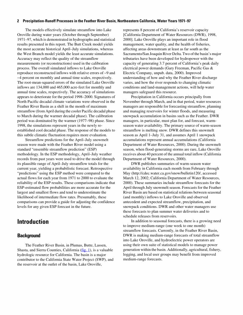
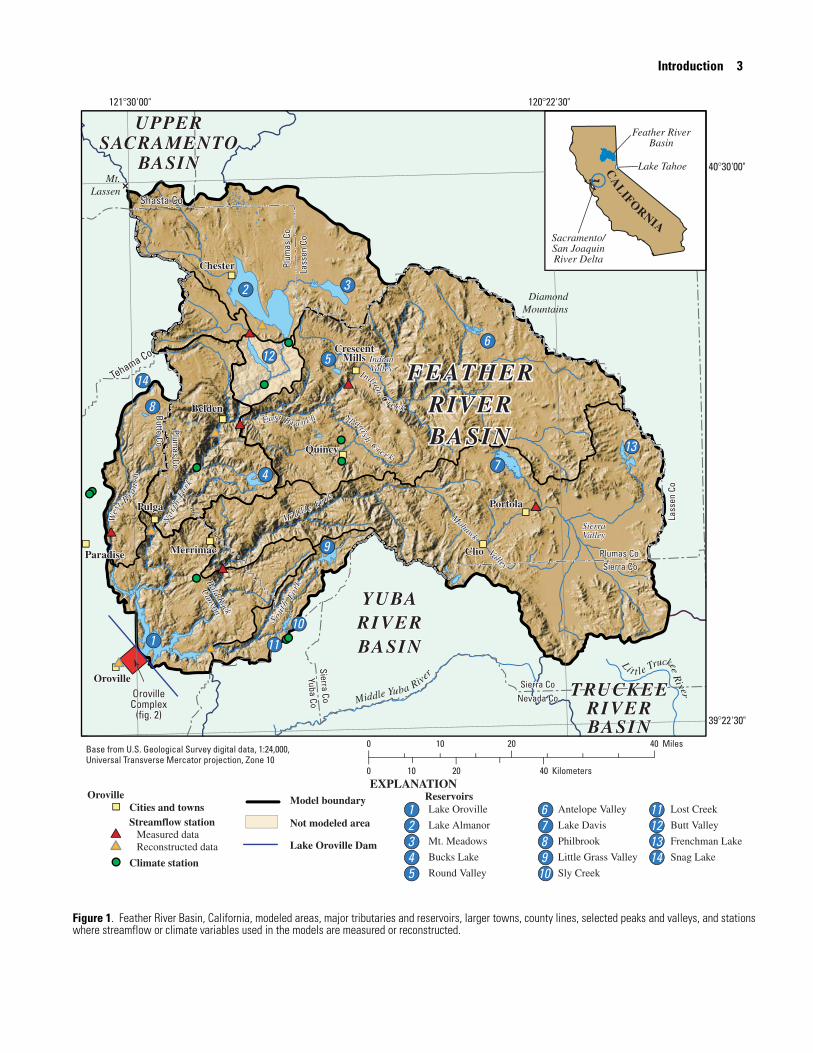


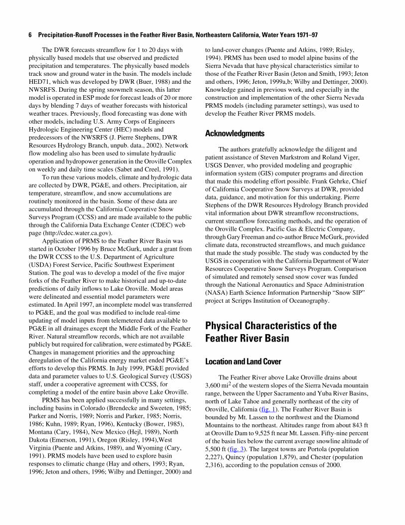
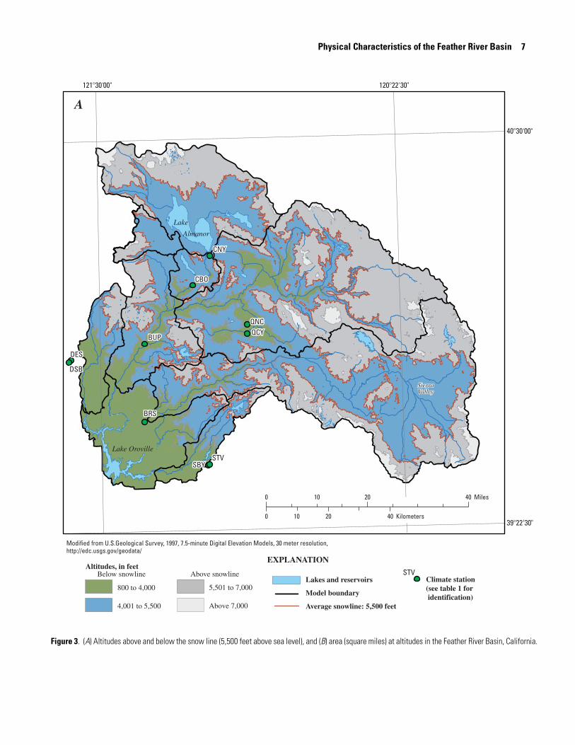

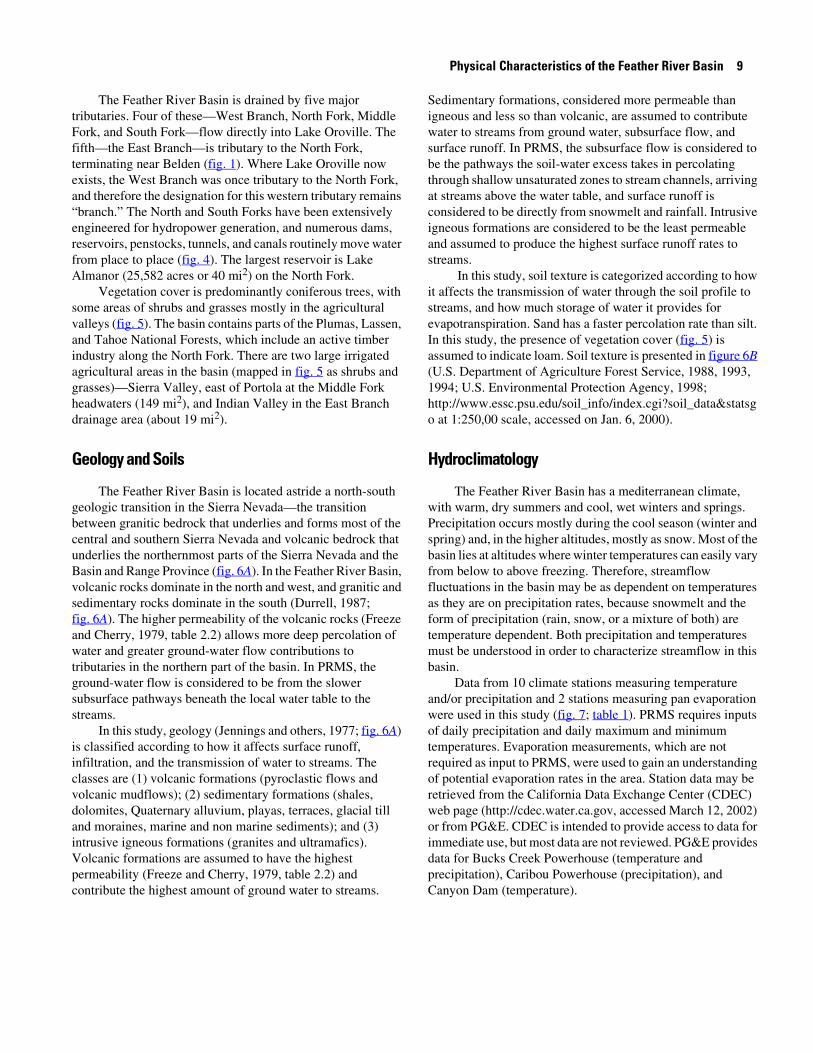
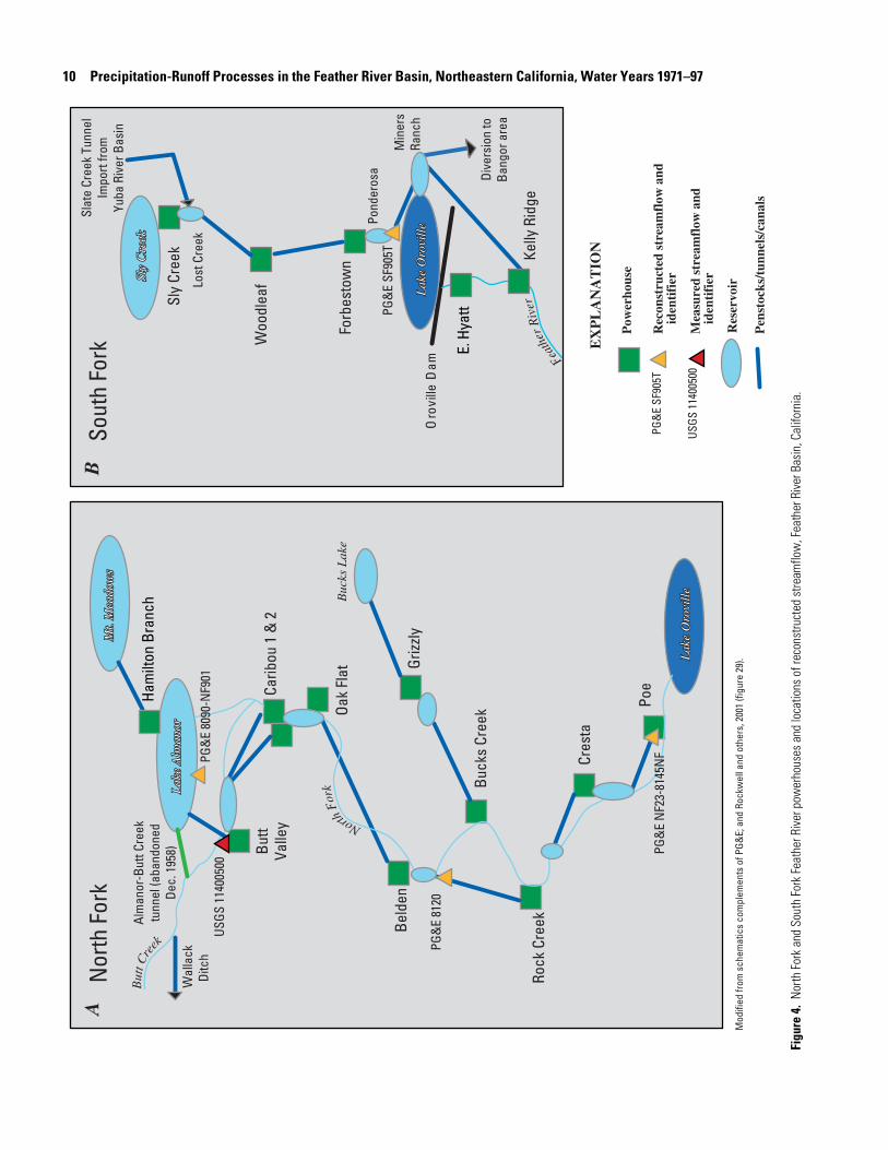
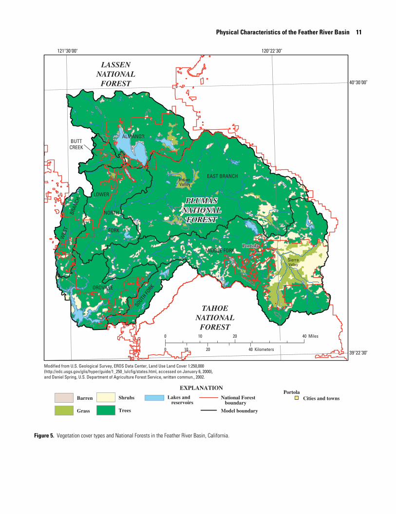
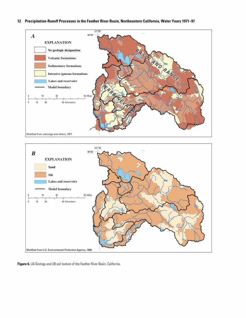
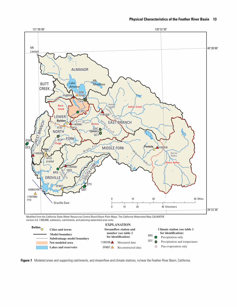

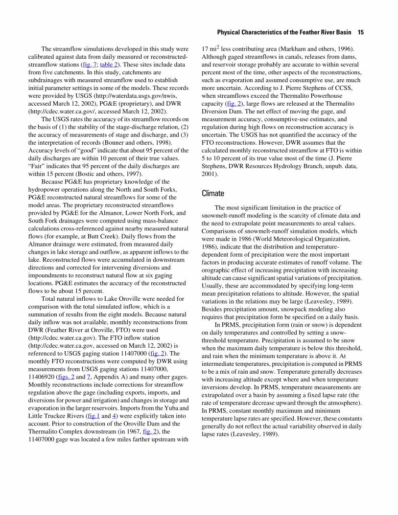

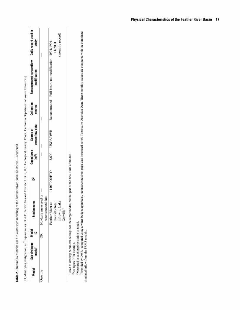

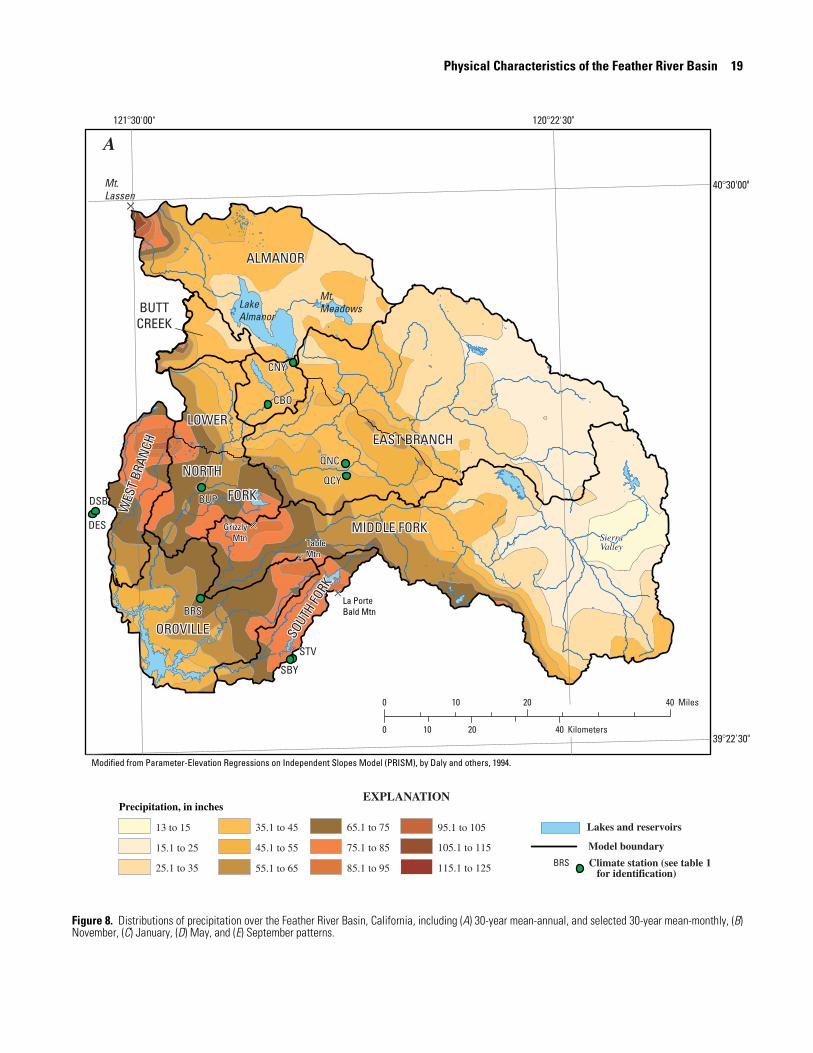
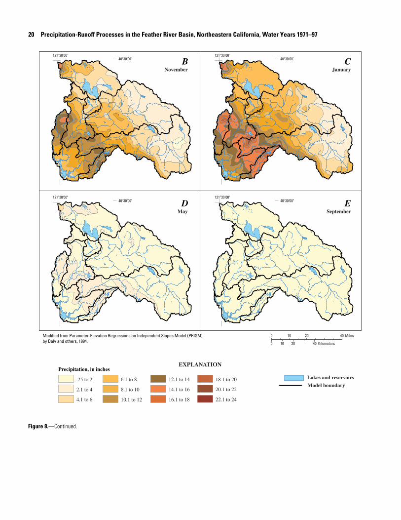
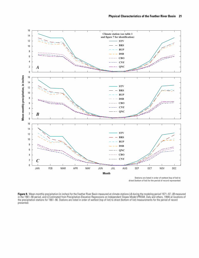
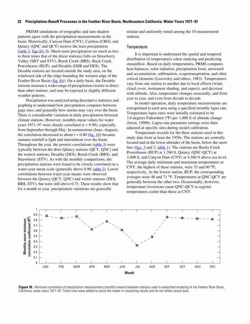
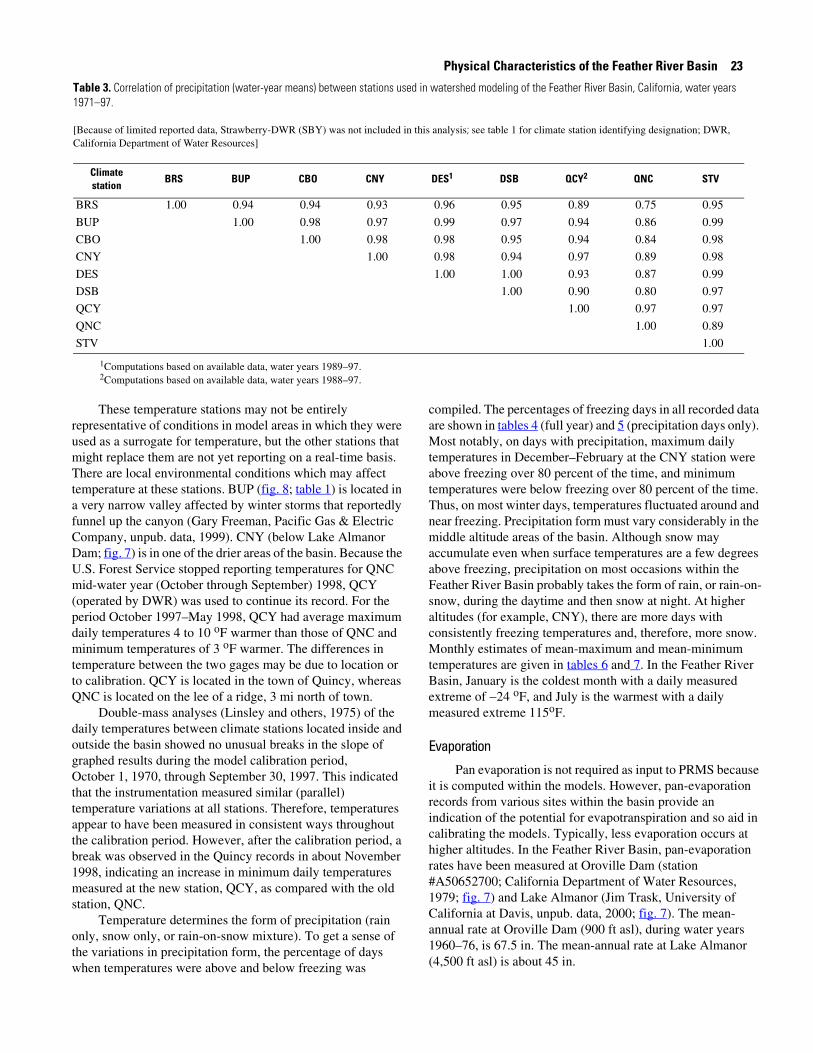

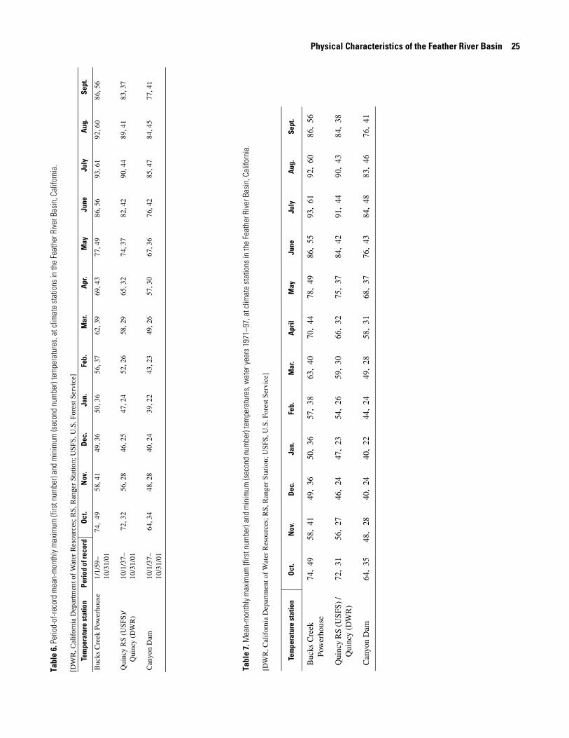
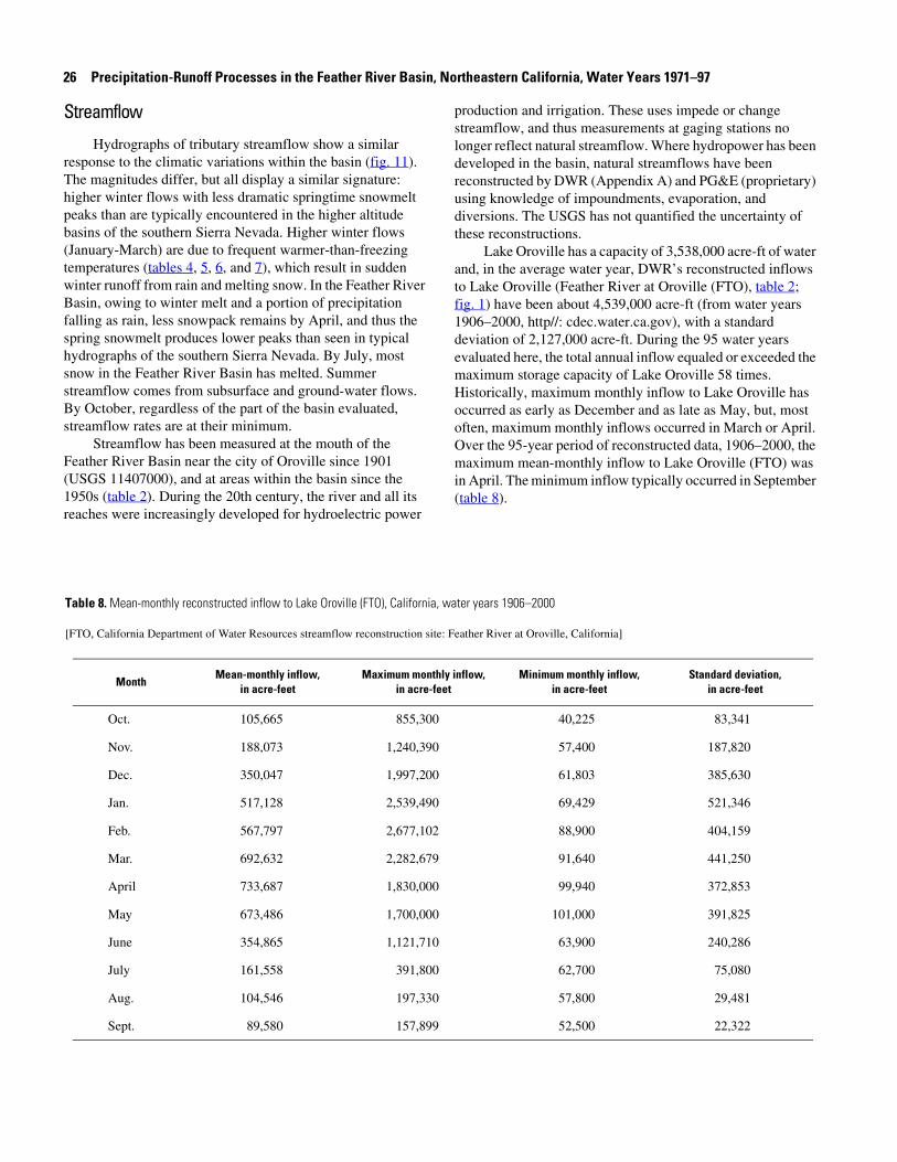
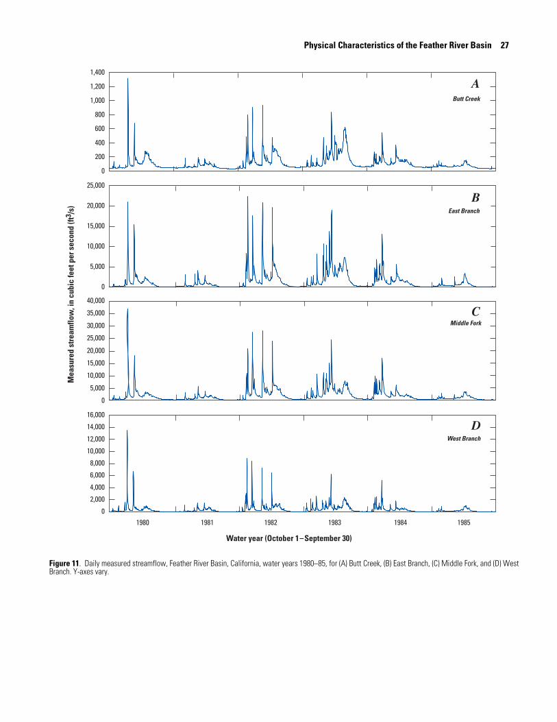

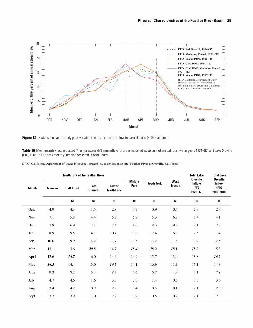
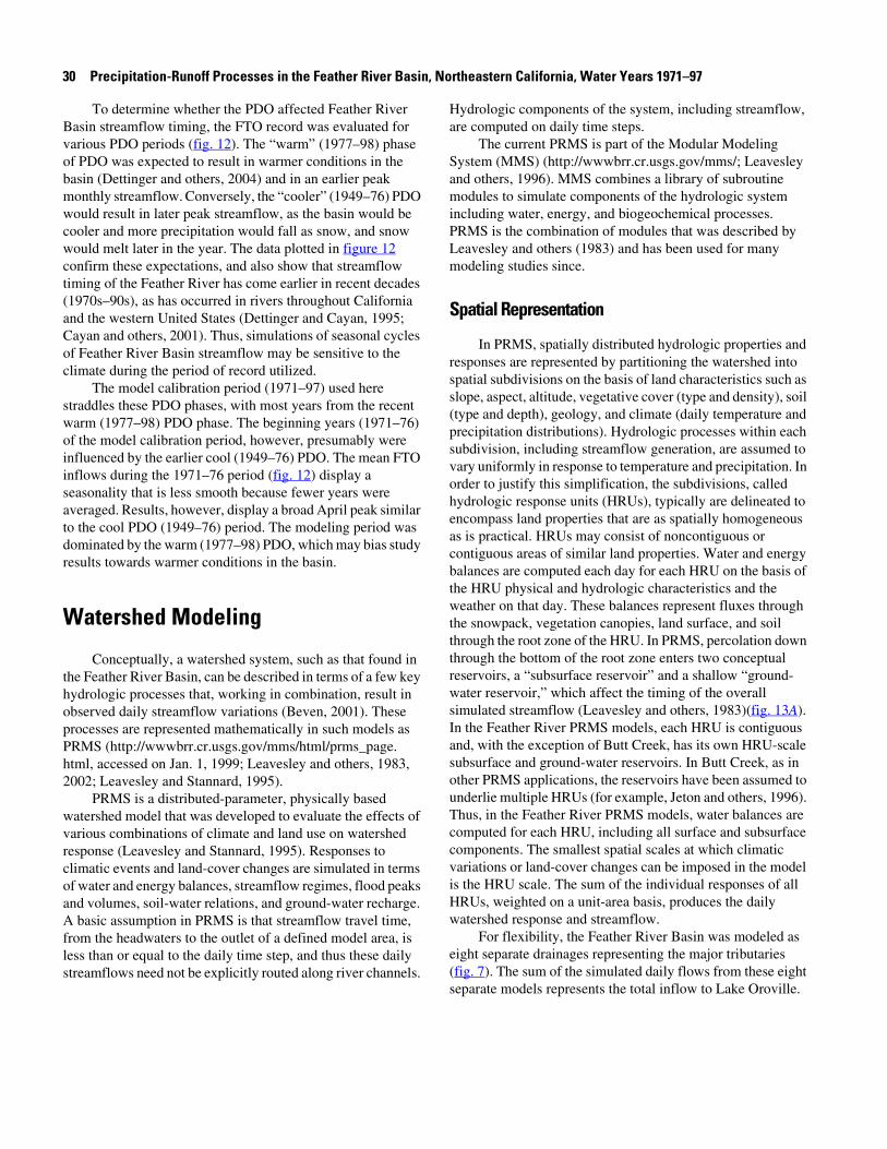
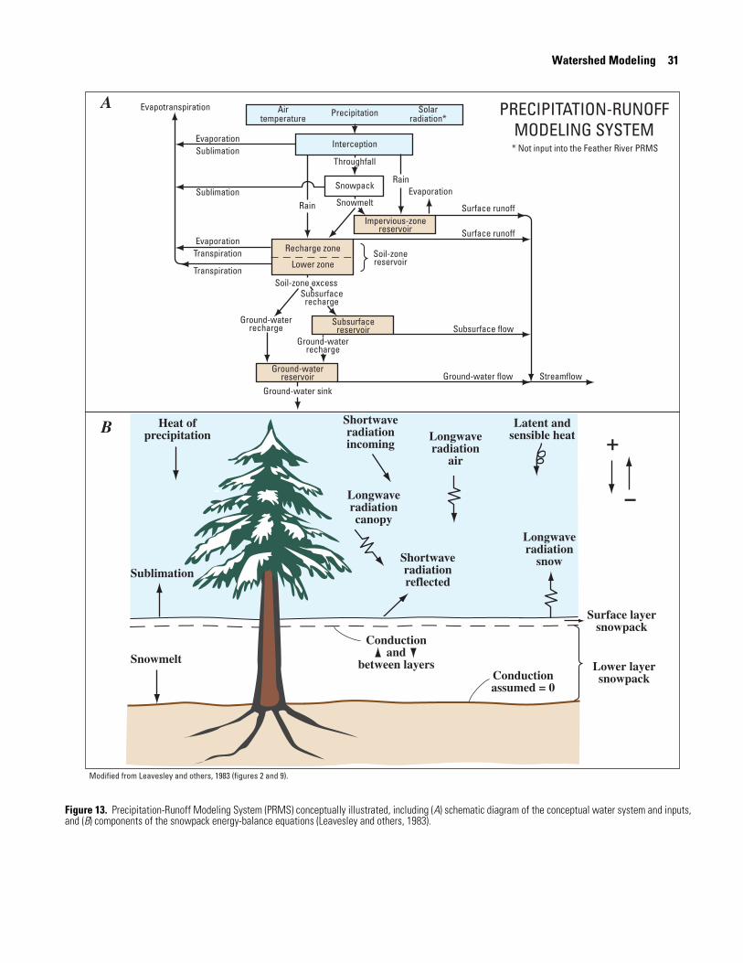


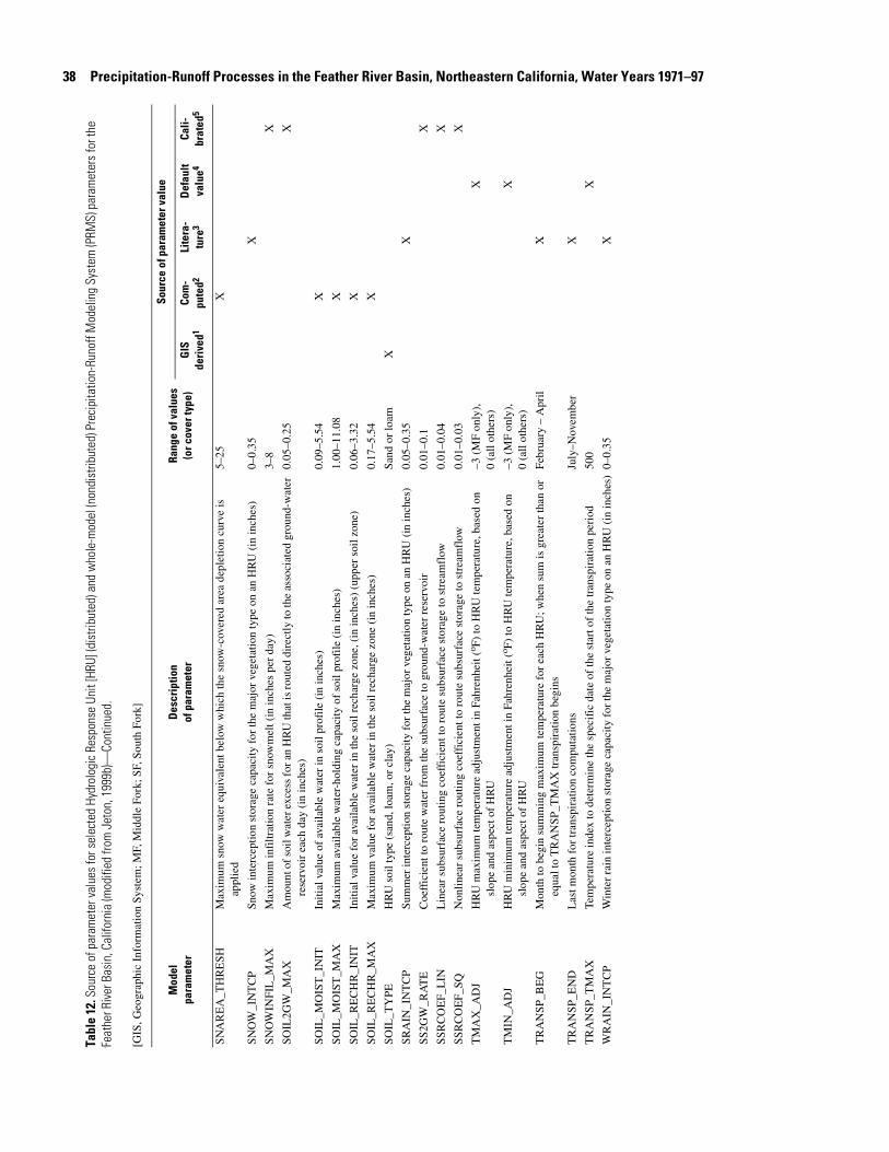
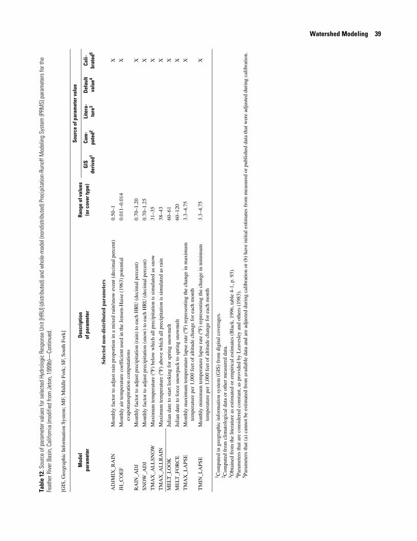
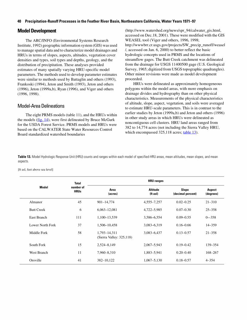

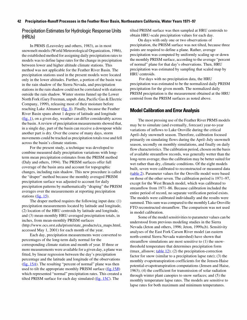
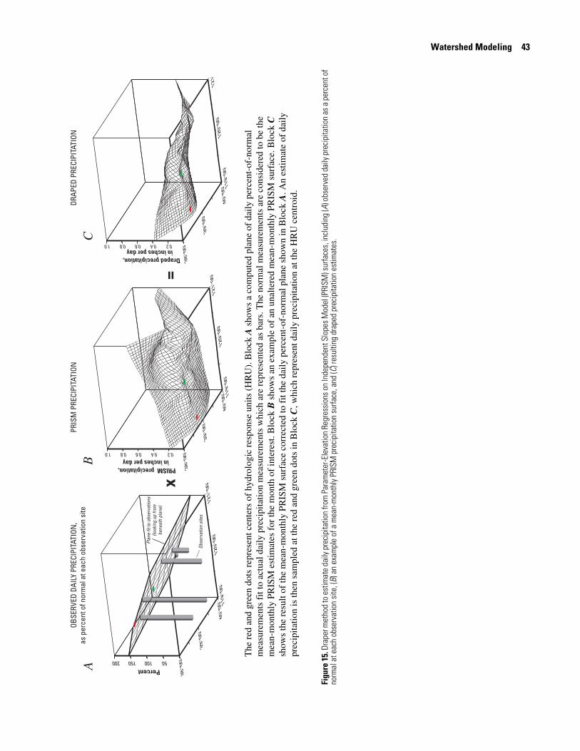
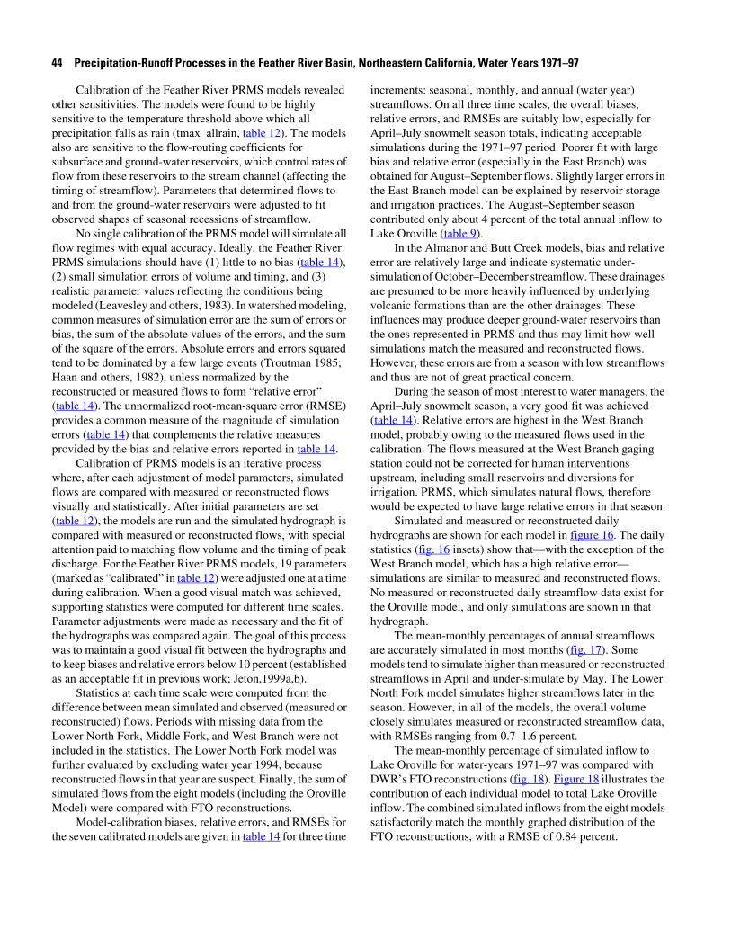

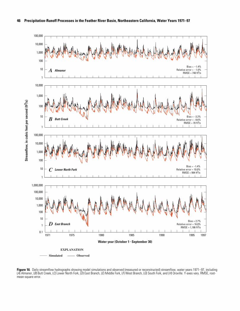
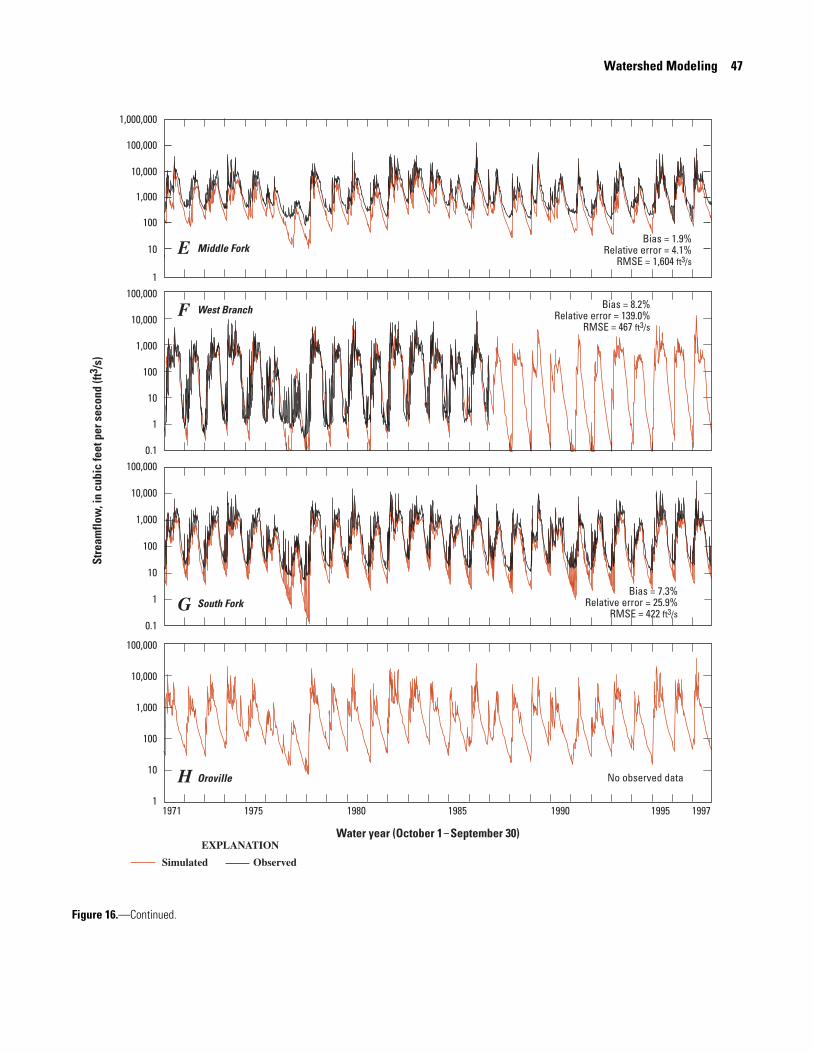
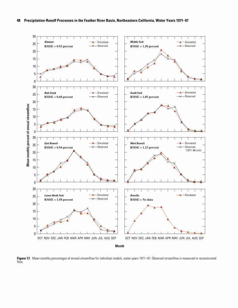
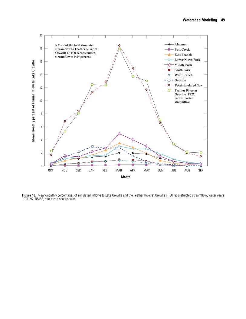

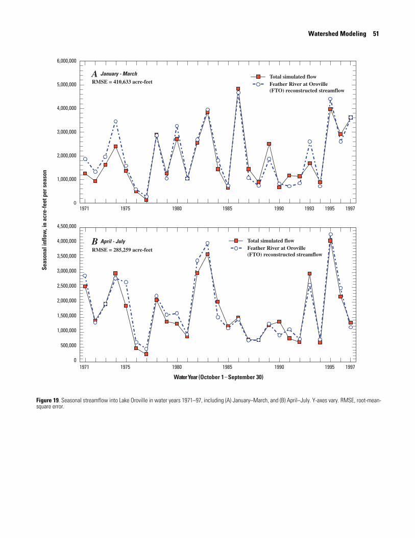


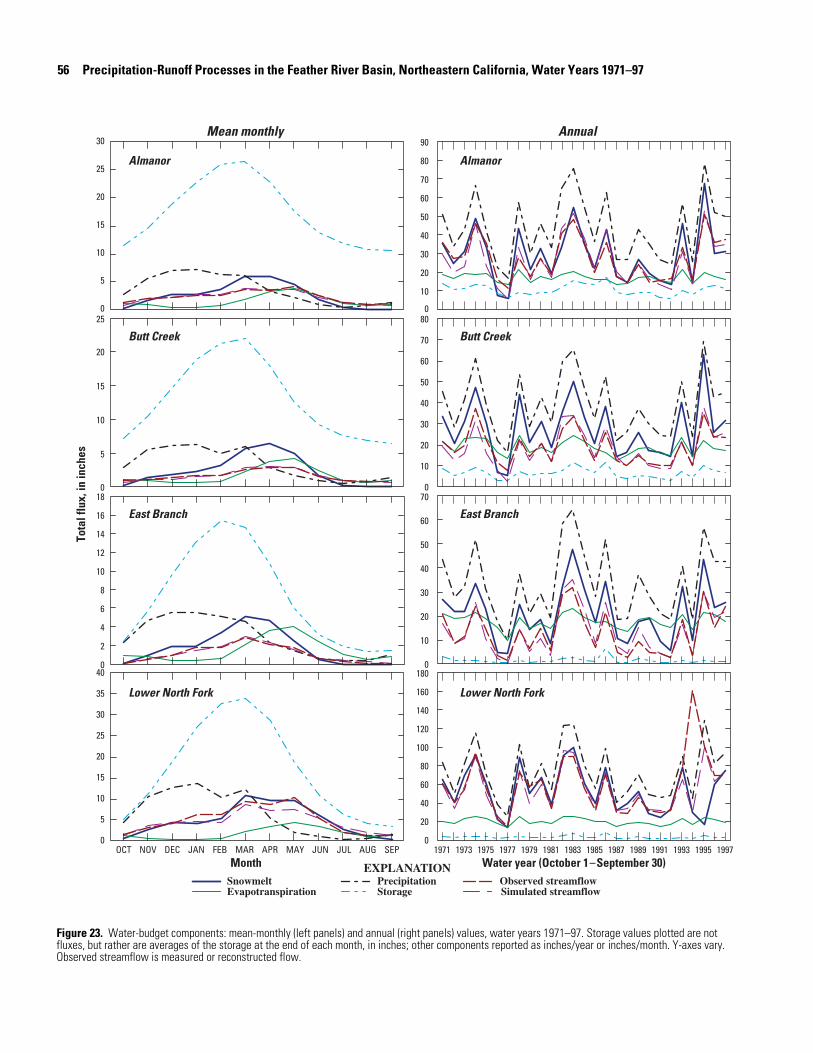
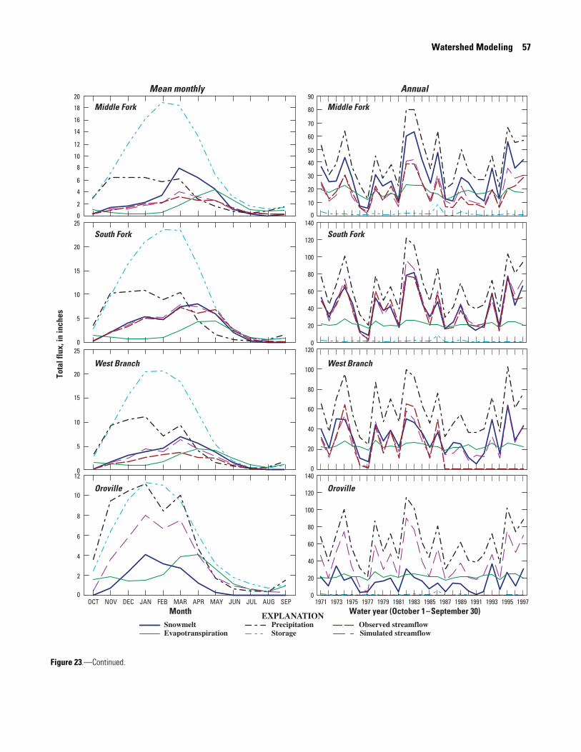
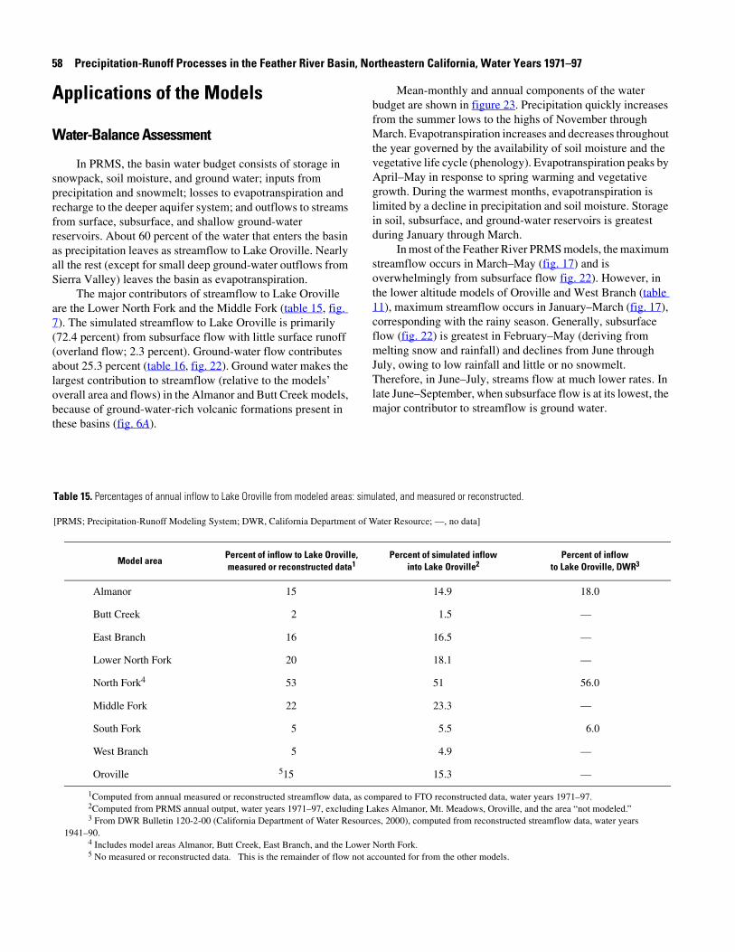


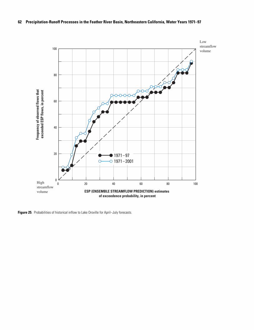


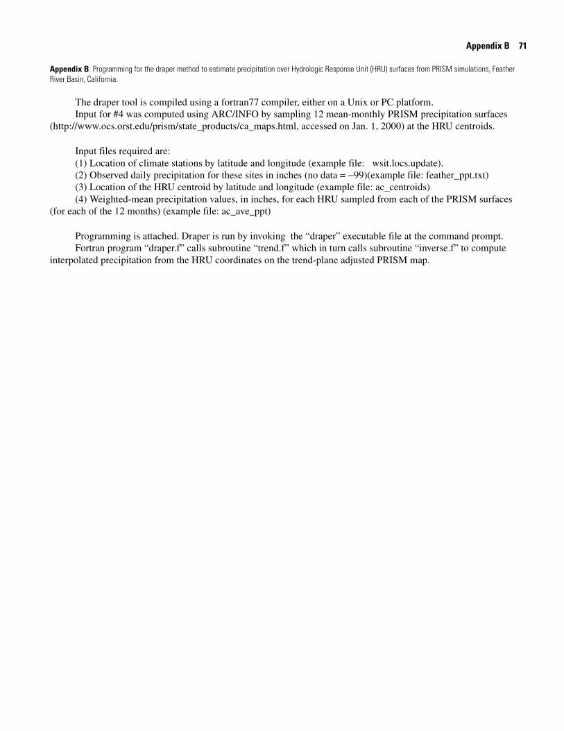
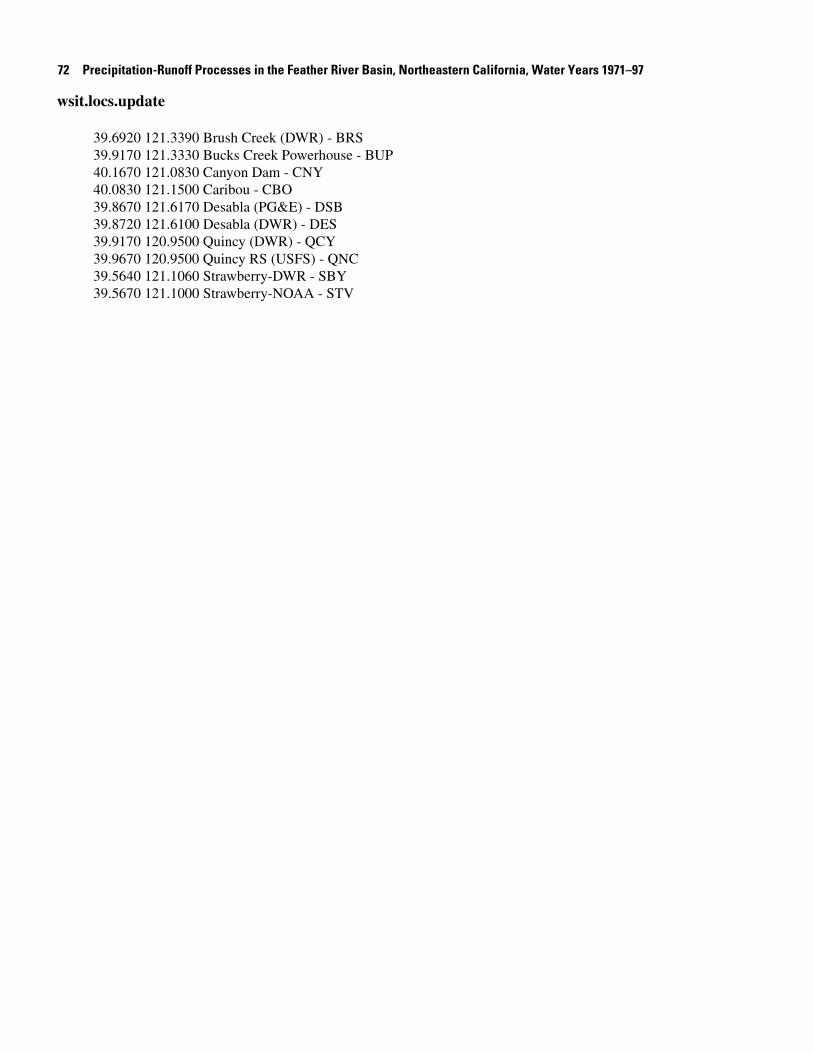

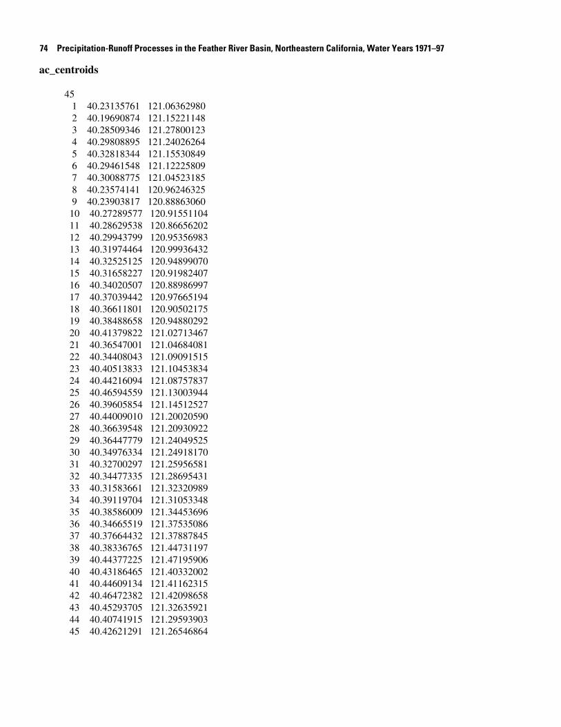
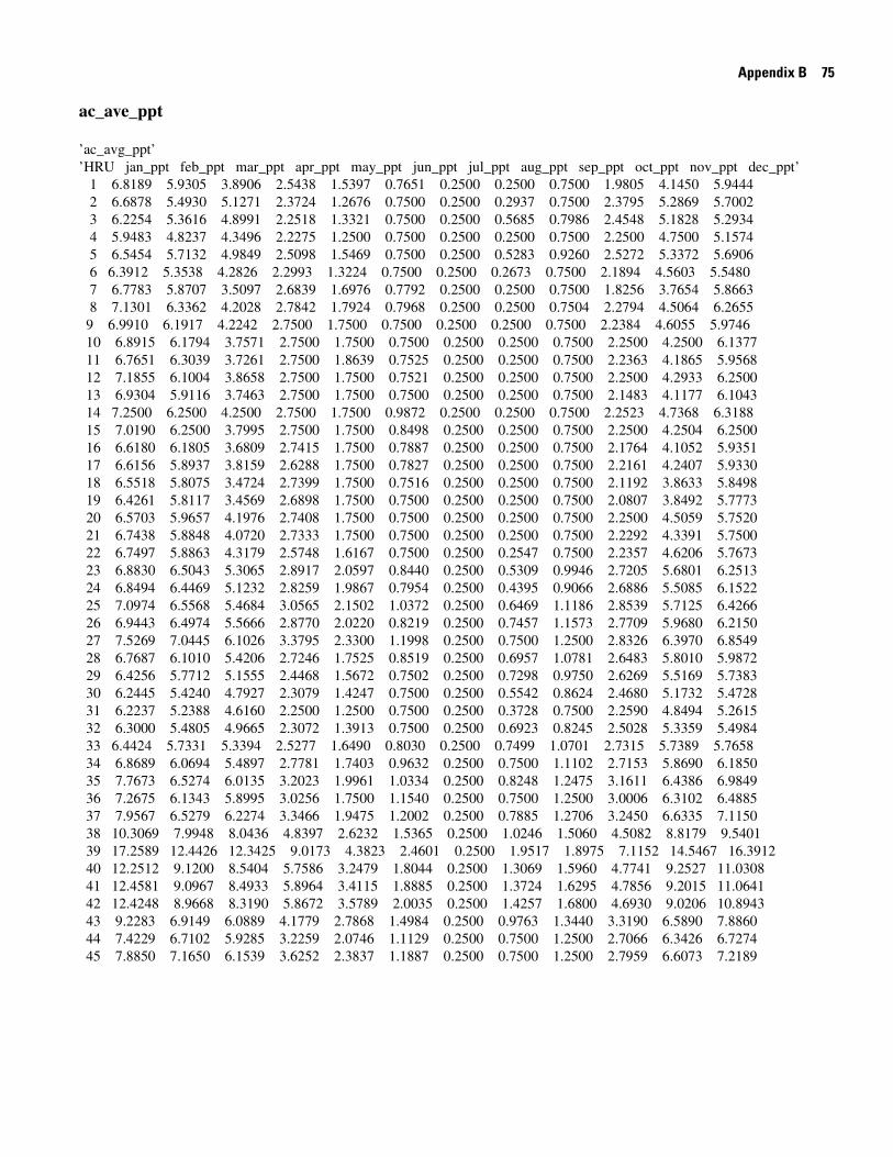


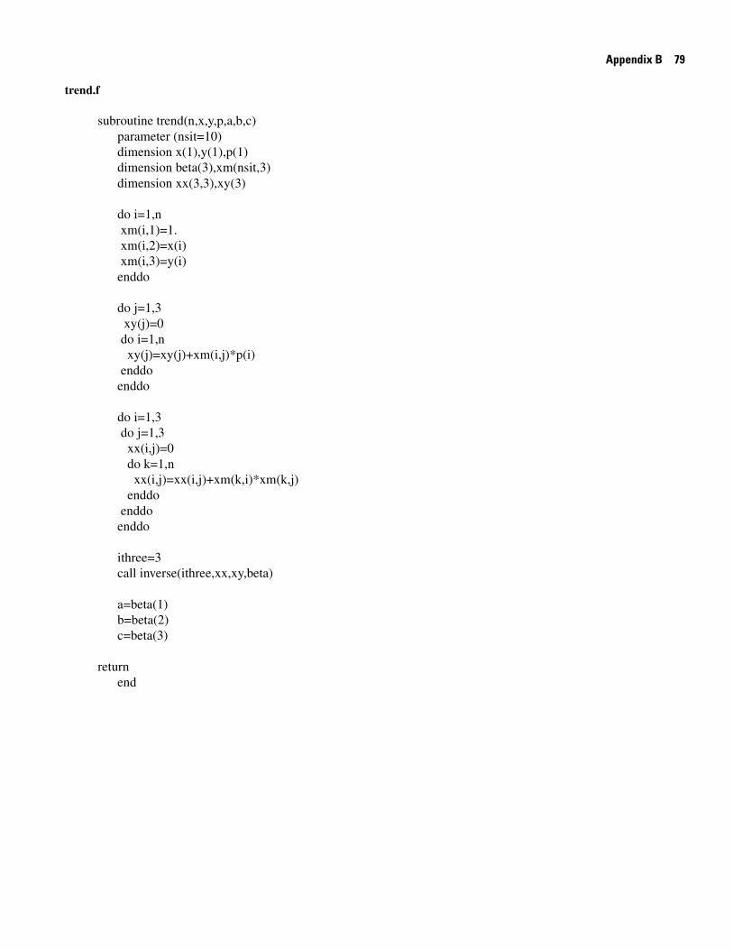
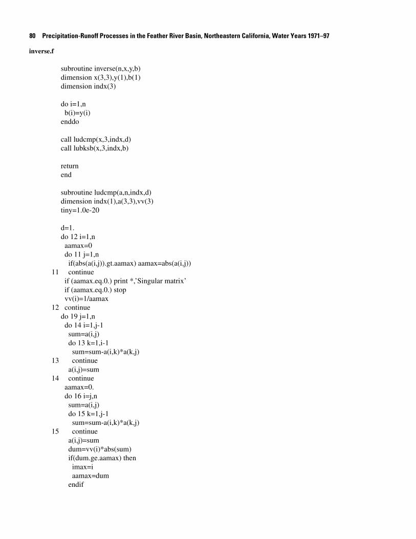
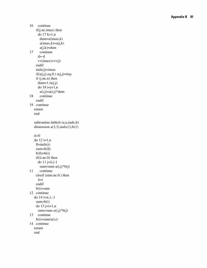


![The history of investigation of salt water inflows into ...€¦ · runoff (428 km3 ) + precipitation (237 km3) – evaporation (184 km3)] is dominated by runoff because precipitation](https://static.documents.pub/doc/80x56/5f7cf0ff5aeed811df507c76/the-history-of-investigation-of-salt-water-inflows-into-runoff-428-km3-.jpg)


