Precoding and Signal Shaping

for Digita 1 Transmission

Robert F. H. Fischer

IEEE The Institute of Electrical and Electronics Engineers, Inc., New York

A JOHN WILEY & SONS, INC., PUBLICATION

This Page Intentionally Left Blank

Precoding and Signal Shaping

for Digital Transmission

This Page Intentionally Left Blank

Precoding and Signal Shaping

for Digita 1 Transmission

Robert F. H. Fischer

IEEE The Institute of Electrical and Electronics Engineers, Inc., New York

A JOHN WILEY & SONS, INC., PUBLICATION

This text is printed on acid-free paper. @

Copyright Q 2002 by John Wiley & Sons, Inc., New York. All rights reserved.

Published simultaneously in Canada.

No part of this publication may be reproduced, stored in a retrieval system or transmitted in any form or by any means, electronic, mechanical, photocopying, recording, scanning or otherwise, except as permitted under Section 107 or 108 of the 1976 United States Copyright Act, without either the prior written permission of the Publisher, or authorization through payment of the appropriate per-copy fee to the Copyright Clearance Center, 222 Rosewood Drive, Danvers, MA 01923, (978) 750-8400, fax (978) 750-4744. Requests to the Publisher for permission should be addressed to the Permissions Department, John Wiley & Sons, Inc., 605 Third Avenue, New York, NY 10158-0012, (212) 850-601 1, fax (212) 850-6008, E-Mail: PERMREQ @I WILEY.COM.

For ordering and customer service, call 1-800-CALL WILEY.

Library of Congress Cataloging-in-Publication Data is available.

Fischer, Robert, F. H. Precoding and Signal Shaping for Digital Transmission/

p. cm. Includes bibliographical references and index. ISBN 0-471-224 10-3 (cloth: alk. paper)

Printed in the United States of America

1 0 9 8 7 6 5 4 3 2 1

Contents

Preface

1 Zntroduction 1.1 1.2 Notation and Dejinitions

The Structure of the Book

1.2.1 Signals and Systems 1.2.2 Stochastic Processes 1.2.3 Equivalent Complex Baseband Signals 1.2.4 Miscellaneous

References

2 Digital Communications via Lineac Distorting Channels 2.1 Fundamentals and Problem Description 2.2 Linear Equalization

2.2.1 Zero-Forcing Linear Equalization 2.2.2 2.2.3

2.2.4 MMSE Linear Equalization 2.2.5

A General Property of the Receive Filter MMSE Filtering and the Orthogonality Principle

Joint Transmitter and Receiver Optimization

xi

9 10 14 15 28

32 35 43

V

\

vi CONTENTS

2.3 Noise Prediction and Decision-Feedback Equalization 2.3.1 Noise Prediction 2.3.2 Zero-Forcing Decision-Feedback Equalization 2.3.3 Finite-Length MMSE Decision-Feedback

2.3.4 Injinite-Length MMSE Decision-Feedback

Summary of Equalization Strategies and Discrete- Time Models 2.4.1 Summary of Equalization Strategies 2.4.2 IIR Channel Models 2.4.3 Channels with Spectral Nulls

2.5 Maximum-Likelihood Sequence Estimation 2.5.1 Whitened-Matched-Filter Front-End 2.5.2 Alternative Derivation

Equalization

Equalization 2.4

References

3 Precoding Schemes 3,l Preliminaries 3.2 Tomlinson-Harashima Precoding

3.2.1 Precoder 3.2.2 Statistical Characteristics of the Transmit

Signal 3.2.3 Tomlinson-Harashima Precoding for Complex

Channels 3.2.4 Precoding for Arbitrary Signal Constellations 3.2.5 Multidimensional Generalization of

Tomlinson-Harashima Precoding 3.2.6 Signal-to-Noise Ratio 3.2.7 Combination with Coded Modulation 3.2.8 Tomlinson-Harashima Precoding and

Feedback Trellis Encoding 3.2.9 Combination with Signal Shaping

3.3.1 Precoder and Inverse Precoder 3.3.2 Transmit Power and Signal-to-Noise Ratio 3.3.3 Combination with Signal Shaping 3.3.4 Straightforward Combination with Coded

3.3.5 Combined Coding and Precoding

3.3 Flexible Precoding

Modulation

49 49 59

77

85

96 96 96

103 108 108 112 116

123 124 127 127

129

135 140

141 142 144

148 150 152 152 155 157

157 161

CONTENTS vii

3.3.6 Spectral Zeros Summary and Comparison of Precoding Schemes Finite- Word-Length Implementation of Precoding Schemes 3.5.1 Two’s Complement Representation 3.5.2 Fixed-Point Realization of Tomlinson-

3.4 3.5

Harashima Precoding 3.6 Nonrecursive Structure for Tomlinson-Harashima

Precoding 3.6.1 Precoding for IIR Channels 3.6.2 Extension to DC-free Channels

3.7 Information-Theoretical Aspects of Precoding 3.7.1

3.7.2 References

Precoding Designed According to MMSE Criterion MMSE Precoding and Channel Capacity

4 Signal Shaping 4.1 Introduction to Shaping

4.1.1 Measures of Performance 4.1.2 4.1.3 Ultimate Shaping Gain

4.2.1 Lattices, Constellations, and Regions 4.2.2 Perfomance of Shaping and Coding 4.2.3 Shaping Properties of Hyperspheres 4.2.4 Shaping Under a Peak Constraint 4.2.5 Shaping on Regions 4.2.6 AWGN Channel and Shaping Gain

4.3.1 Preliminaries 4.3.2 4.3.3 4.3.4 Arbitrary Frame Sizes 4.3.5 General Cost Functions 4.3.6 Shell Frequency Distribution

4.4.1 Motivation 4.4.2 Trellis Shaping on Regions

Optimal Distribution for Given Constellation

4.2 Bounds on Shaping

4.3 Shell Mapping

Sorting and Iteration on Dimensions Shell Mapping Encoder and Decoder

4.4 Trellis Shaping

169 171

181 181

185

195 195 197 199

199 203 21 1

21 9 220 223 224 22 7 229 229 232 235 242 24 7 253 258 258 259 266 2 70 2 72 2 76 282 282 289

viii CONTENTS

4.4.3 Practical Considerations and Performance 4.4.4 4.4.5 Spectral Shaping 4.4.6 Further Shaping Properties Approaching Capacity by Equiprobable Signaling 4.5.1 4.5.2 Nonuniform Constellations-Warping 4.5.3 Modulus Conversion

Shaping, Channel Coding, and Source Coding

4.5 AWGN Channel and Equiprobable Signaling

References

5 Combined Precoding and Signal Shaping 5.1 Trellis Precoding

5.1.1 Operation of Trellis Precoding 5.1.2 Branch Metrics Calculation

5.2 Shaping Without Scrambling 5.2.1 Basic Principle 5.2.2 5.2.3 Precoding and Shaping under Additional Constraints 5.3.1 Preliminaries on Receiver-Side Dynamics

Restriction 5.3.2 Dynamics Limited Precoding 5.3.3 Dynamics Shaping 5.3.4 Reduction of the Peak-to-Average Power Ratio Geometrical Interpretation of Precoding and Shaping 5.4.1 Combined Precoding and Signal Shaping 5.4.2 Limitation of the Dynamic Range

5.5 Connection to Quantization and Prediction References

Decoding and Branch Metrics Calculation Perfonnance of Shaping Without Scrambling

5.3

5.4

Appendix A Wirtinger Calculus A.1 Real and Complex Derivatives A. 2 Wirtinger Calculus

A.2.1 Examples A.2.2 Discussion

A.3.1 Examples A.3.2 Discussion

A.3 Gradients

References

297 307 309 31 6 31 8 31 8 321 328 334

341 344 345 346 356 356 357 361 369

369 3 70 377 384 392 392 394 397 400

405 406 407 408 41 0 41 1 41 1 41 2 41 3

CONTENTS ix

Appendix B Parameters of the Numerical Examples B. 1 Fundamentals of Digital Subscriber Lines B.2 Single-Pair Digital Subscriber Lines B.3 Asymmetric Digital Subscriber Lines References

Appendix C Introduction to Lattices C. 1 Dejnition of Lattices C.2 C.3 ModiJications of Lattices C.4 Sublattices, Cosets, and Partitions C.5 References

Some Important Parameters of Lattices

Some Important Lattices and Their Parameters

Appendix D Calculation of Shell Frequency Distribution D. 1 Partial Histograms 0 . 2 0 . 3 Frequencies of Shells References

Partial Histograms for General Cost Functions

Appendix E Precoding for MIMO Channels E.l Centralized Receiver

E. 1.1 Multiple-Input/Multiple-Output Channel E. 1.2 E.1.3 Matrix DFE E. 1.4 Tomlinson-Harashima Precoding

E.2 Decentralized Receivers E.2.1 Channel Model E.2.2 Centralized Receiver and Decision-Feedback

E.2.3 Decentralized Receivers and Precoding

E.3.1 ISI Channels E.3.2 Application of Channel Coding E.3.3 Application of Signal Shaping E.3.4 Rate and Power Distribution

Equalization Strategies for MIMO Channels

Equalization

E.3 Discussion

References

Awwendix F List of Svmbols. Variables. and Acronvms

41 5 415 41 7 41 8 420

421 421 425 428 430 434 437

439 440 444 445 453

455 456 456 457 459 460 465 465

466 466 468 468 469 4 70 4 70 4 71

4 75

R l Important Sets of Numbers and Constants 4 75

R4 Acronyms 4 79

E 2 Transforms, Operators, and Special Functions 4 76 E 3 Important Variables 4 78

Index 483

Preface

This book is the outcome of my research and teaching activities in the field of fast digital communication, especially applied to the subscriber lines network, over the last ten years. It is primarily intended as a textbook for graduate students in electrical engineering, specializing in communications. However, it may also serve as a refer- ence book for the practicing engineer. The reader is expected to have a background in engineering and to be familiar with the theory of signals and systems-the basics of communications, especially digital pulse-amplitude-modulated transmission, are presumed.

The scope of this book is to explain in detail the fundamentals of digital trans- mission over linear distorting channels. These channels-called intersymbol-inter- ference channels-disperse transmitted pulses and produce long-sustained echos. After having reviewed classical equalization techniques, we especially focus on the applications of precoding. Using such techniques, channels are preequalized at the transmitter side rather than equalized at the receiver. The advantages of such strate- gies are highlightened, and it is shown how this can be done under a number of additional constraints. Furthermore, signal shaping algorithms are discussed, which can be applied to generate a wide range of desired properties of the transmitted or received signal in digital transmission. Typically, the most interesting property is low average transmit power. Combining both techniques, very powerful and flexible schemes can be established. Over recent years, such schemes have attracted more and more interest and are now part of a number of standards in the field of digital transmission systems.

X i

xii PREFACE

I wish to thank everyone who supported me during the preparation of this book. In particular, I am deeply indebted to my academic teacher Prof. Dr. Johannes Huber for giving me the opportunity to work in his group, for his encouragement, his valuable advice in writing this book, and for the freedom he gave me to complete my work. The present book is strongly influenced by him and his courses that I had the chance to attend.

Many thanks to all proofreaders for their diligent review, helpful comments, and suggestions. Especially, I would like to acknowledge Dr. Stefan Muller-Weinfurter for his detailed counsel on earlier versions of the manuscript, and Prof. Dr. Jo- hann Weinrichter at the Technical University of Vienna for his support. Many thanks also to Lutz Lampe and Christoph Windpassinger for their critical reading. All remaining inadequateness and errors are not due to their fault, but because of the ignorance or unwillingness of the author.

Finally, I express thanks to all colleagues for the pleasant and companionable atmosphere at the Lehrstuhl fur Informationsiibertragung, and the entire Telecom- munications Laboratory at the University of Erlangen-Nurnberg.

ROBERT F. H. FISCHEK

Erlangeri, Germany

Muy 2002

1 Introduction

eliable digital transmission is the basis of what is commonly called the “infor- mation age.” Especially the boom of the Internet and its tremendous growth are boosting the ubiquity of digital information. Text, graphics, video, and

sound are certainly the most visible examples. Hence, high-speed access to the global networks is one of the key issues that have to be solved. Meanwhile not only business sites are interested in fast access, but also private households increasingly desire to become connected, yearning for ever-increasing data rates.

Of all the network access technologies currently under discussion, the digital Subscriber lines (DSL) technique is probably the most promising one. The copper subscriber lines, which were installed over the last decades, were only used for the plain old telephone system (POTS) or at most for integrated Services digital - network (ZSDN) services. But dial-up (voice;band) modems with data rates well below 50 kbitsk are only able to whet the appetite for Internet access.

During the 1980s it was realized that this medium can support data rates up to some megabits per second for a very high percentage of subscribers. Owing to its high degree of penetration, the use of copper lines for digital transmission can build an easy-to-install and cost-efficient bridge from today’s analog telephone service to the very high-speed fiber-based communications in the future. Hence, copper is probably the most appealing candidate to solve the “last-mile problem,” i.e., bridging the distance from the central office to the customer’s premises.

Initiated by early research activities and prototype systems in Europe, at the end of the 1980s an the beginning of the 1990s, broad research activities began which led to what is now commonly denoted as digital subscriber lines. Meanwhile a whole

1

family of philosophies and techniques are being designed or are already in practical use. The first instance to be mentioned is high-rate digital Subscriber lines (HDSL), which provide 2.048 Mbits/s (El rate in Europe) or 1.544 Mbits/s (DS 1 rate in North America) in both directions, typically using two wire pairs. HDSL can be seen as the successor of ISDN primary rate access. Contrary to HDSL, which is basically intended for commercial applications, gymmetric digital Subscriber lines (ADSL) are aimed at private usage. Over a single line, ADSL offers up to 6 Mbits/s from the central office to the subscriber and a reverse channel with some hundred kbitds- hence the term asymmetric. Interestingly, ADSL can coexist with POTS or ISDN on the same line. Standardization activities are presently under way for Single-pair digital Subscriber lines (SDSL) (sometimes also called symmetric DSL), which will support 2.312 Mbits/s in both directions while occupying only a single line. Finally, - very high-rate digital Subscriber lines (VDSL) have to be mentioned. If only some hundred meters, instead of kilometers, have to be bridged, the copper line can carry up to 50 Mbits/s or even more.

The purpose of this book is to explain in detail the fundamentals of digital transmis- sion over channels which disperse the transmitted pulse and produce long-sustained echos. We show how to equalize such channels under a number of additional con- straints. Thereby, we focus onprecoding techniques, which do preequalization at the transmitter side, and which in fact enable the use of channel coding. Moreover, signal shaping is discussed, which provides further gains, and which can be applied to gen- erate a wide range of desired properties for transmit or received signal. Combining both strategies, very powerful and flexible schemes can be established.

Even though most examples are chosen from the DSL world, the concepts of equalization and shaping are applicable to all scenarios where digital transmission over distorting channels takes place. Examples are power-line communication with its demanding transmission medium, or even mobile communications, where the time-varying channel is rather challenging.

We expect the reader to have an engineering background and to be familiar with the theory of signals and systems, both for the continuous-time and discrete-time case. This also includes knowledge of random processes and their description in the time and frequency domains. Also, the basics of communications, especially digital pulse-amplitude-modulated transmission, are assumed.

THE STRUCTURE OF THE BOOK 3

1.1 THE STRUCTURE OF THE BOOK

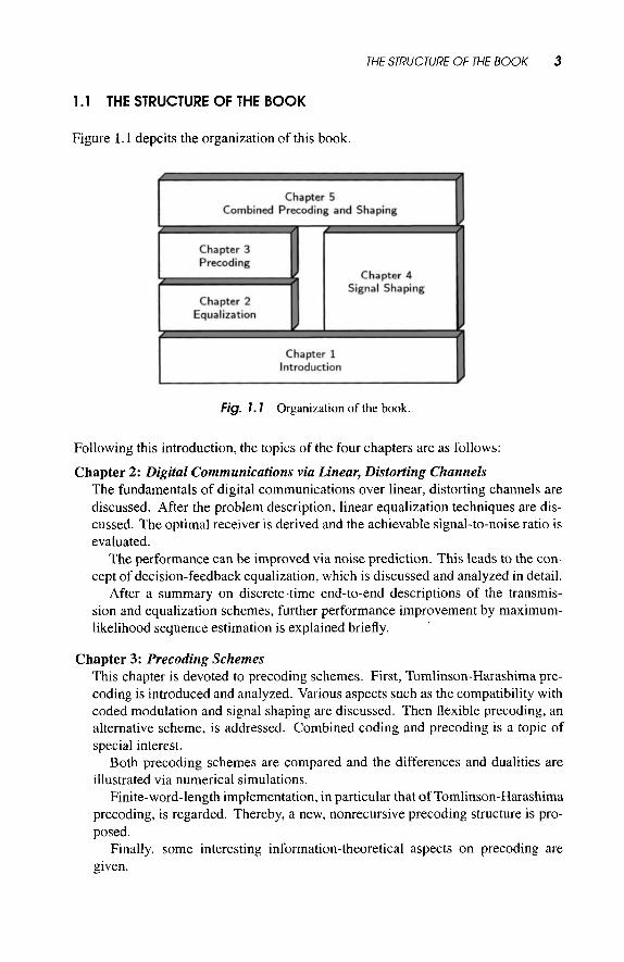
Figure 1.1 depcits the organization of this book.

Fig. 1. I Organization of the book.

Following this introduction, the topics of the four chapters are as follows:

Chapter 2: Digital Communications via Linear, Distorting Channels The fundamentals of digital communications over linear, distorting channels are discussed. After the problem description, linear equalization techniques are dis- cussed. The optimal receiver is derived and the achievable signal-to-noise ratio is evaluated.

The performance can be improved via noise prediction. This leads to the con- cept of decision-feedback equalization, which is discussed and analyzed in detail.

After a summary on discrete-time end-to-end descriptions of the transmis- sion and equalization schemes, further performance improvement by maximum- likelihood sequence estimation is explained briefly.

Chapter 3: Precoding Schemes This chapter is devoted to precoding schemes. First, Tomlinson-Harashima pre- coding is introduced and analyzed. Various aspects such as the compatibility with coded modulation and signal shaping are discussed. Then flexible precoding, an alternative scheme, is addressed. Combined coding and precoding is a topic of special interest.

Both precoding schemes are compared and the differences and dualities are illustrated via numerical simulations.

Finite-word-length implementation, in particular that of Tomlinson-Harashima precoding, is regarded. Thereby, a new, nonrecursive precoding structure is pro- posed.

Finally, some interesting information-theoretical aspects on precoding are given.

4 lNJRODUCJlON

Chapter 4: Signal Shaping In this chapter, signal shaping, i.e., the generation of signals with least average power, is discussed. By using the signal points nonequiprobable, a power reduc- tion is possible without sacrificing performance. The differences and similarities between shaping and source or channel coding are studied. Then, performance bounds on shaping are derived.

Two shaping schemes are explained in detail: shell mapping and trellis shap- ing. The shaping algorithms are motivated and their performance is covered by numerical simulations.

In the context of trellis shaping, the control of the power spectral density is studied as an example for general shaping aims.

The chapter closes with the optimization of the signal-point spacing rather than resorting to nonequiprobable signaling.

Chapter 5: Combined Precoding and Signal Shaping Combined precoding and signal shaping is addressed. In addition to preequaliza- tion of the intersymbol-interference channel, the transmit signal should have least average power.

In particular, the combination of Tomlinson-Harashima precoding and trellis shaping, called trellis precoding, is studied. Then, shaping without scrambling is presented, which avoids the disadvantages of trellis precoding and, without changing the receiver, can directly replace Tomlinson-Harashima precoding.

Besides average transmit power, further signal parameters may be controlled by shaping. Specifically, a restriction of the dynamic range at the receiver side and a reduction of the peak-to-average power ratio of the continuous-time transmit signal, are considered.

After a geometrical interpretation of combined precoding and shaping schemes is given, the duality of precoding/shaping to source coding of sources with memory is briefly discussed.

Appendices: Appendix A summarizes the Wirtinger Calculus, which is a handy tool for opti- mization problems depending on one or more complex-valued variables.

The Parameters of the Numerical Simulations given in this book are summa- rized in Appendix B.

In Appendix C, an Introduction to Lattices, which are a powerful concept when dealing with precoding and signal shaping, is given.

The Calculation of Shell Frequency Distribution in shell-mapping-based transmission schemes is illustrated in Appendix D.

Appendix E generalizes precoding schemes and explains briefly Precoding for MZMO Channels.

Finally, in Appendix F a List of Symbols, Variables, and Acronyms is given.

Note, the bibliography is given individually at the end of each chapter.

NOTATION AND DEFINITIONS 5

1.2 NOTATION AND DEFINITIONS

1.2.1 Signals and Systems

Continuous-time signals are denoted by lowercase letters and are functions of the continuous-time variable t E IR (in seconds), e.g., s ( t ) . Without further notice, all signals are allowed to be complex-valued, i.e., represent real signals in the equivalent complex baseband. By sampling a continuous-time signal-taking s [k ] = s (kT)- where T is the sampling period, we obtain a sequence of samples s [ k ] , numbered by the discrete-time index k E Z written in square brackets. If the whole sequence is regarded, we denote it as ( ~ [ k ] ) .

The Fourier transform of a time-domain signal z ( t ) is displayed as a function of the frequency f E IR (in hertz) and denoted by the corresponding capital letter. Transform and its inverse, respectively, are defined as

X ( f ) = F{z(t)} 7 z ( t )e -J2" f t d t , (1.2. la)

z ( t ) = . F ' { X ( f ) } 1 X ( f ) e j a n f t df . ( 1.2.1 b)

The correspondence between the time-domain signal z ( t ) and its Fourier transform X (f ) is denoted briefly as

A

-m co

-m

z ( t ) - X U ) . (1.2.2)

The z-transform of the sequence ( z [ k ] ) and its inverse are given as

X ( 2 ) = 2 { z [ k ] } !i Cz[k] Z-k , (1.2.3a) k

1 z [ k ] = 2 - ' { X ( z ) } 4 - / X ( Z ) & ' dz , (1.2.3b)

27TJ

for which we use the short denomination z [ k ] - X ( z ) , too.

signal dd) [ k ] = z(kT) and that of the continuous-time signal z ( t ) are related by Regarding the Fourier pair (1.2.2), the spectrum X(d) (e j2 . r r fT ) of the sampled

A

(1.2.4)

Because the spectrum is given by the z-transform, evaluated on the unit circle, we use the denomination e jaTfT as its argument. Moreover, this emphasizes the periodicity of the spectrum over frequency.

1.2.2 Stochastic Processes

In communications, due to the random nature of information, all signals are members of a stochastic process. It is noteworthy that we do not use different notations when

6 lNTRODUCTlON

dealing with the process or a single sample functiodsequence thereof. Expectation is done across the ensemble of functions belonging to the stochastic process and denoted by E { .} .

Autocorrelation and cross-correlation sequences of (wide-sense) stationary pro- cesses shall be defined as follows

$ ~ z [ K ] = E { ~ [ k + K ] .2*[k]} , (1.2.5a)

$zy[K] E { Z [ k f K] . y * [ k ] } . (1.2.5b)

The respective quantities for continuous-time processes are defined accordingly. The power spectral density corresponding to the autocorrelation sequence dZ2 [ K ]

of a stationary process is denoted as Q,(eJaTfT), and both quantities are related by

(1.2.6)

When dealing with cyclostationary processes (e.g., the transmit signal in pulse amplitude modulation), the average power spectral density is regarded.

Finally, Pr{ .} stands for the probability of an event. If the random variable 5 is distributed continuously rather than discrete, its distribution is characterized by the probability density function (pdf) fZ(z). In case of random variables z, conditioned on the event y, we give the conditional pdf fz(zly).

1.2.3 Equivalent Complex Baseband Signals

It is convenient to represent (real-valued) bandpass signals' by its corresponding equivalent complex baseband signal, sometimes also called equivalent low-pass signal or complex envelope [Fra69, Tre7 1, ProOl].

Let ZHF ( t ) be a real-valued (high-frequency) signal and XHF (f) its Fourier trans- form, i.e., ~ H F ( t ) 0-0 X H F ( ~ ) . The equivalent complex baseband signal z ( t ) corre- sponding to q F ( t ) is obtained by first going to one-sided spectra, i.e., generating the analytic signal to Z H F ( ~ ) [Pap77], and then shifting the spectrum by the frequency fo, such that the relevant components are located around the origin and appears as a low-pass signal. Usually, when regarding carrier-modulated transmission, the trans- formation frequency fo is chosen equal to the carrier frequency. Mathematically, we have

(1.2.7aj

where X { .} denotes Hilbert transform [Pap77]. Conversely, given the complex baseband representation rc(t), the corresponding real-valued signal is obtained as

z ~ ~ ( t ) = fi Re { z ( t ) . e+jzTfot} . (1.2.7b)

'To be precise, the only requirement for the application of equivalent complex baseband representations is that the signals are real-valued, and hence one half of the spectrum is redundant.

NOTATION AND DEFINITIONS 7

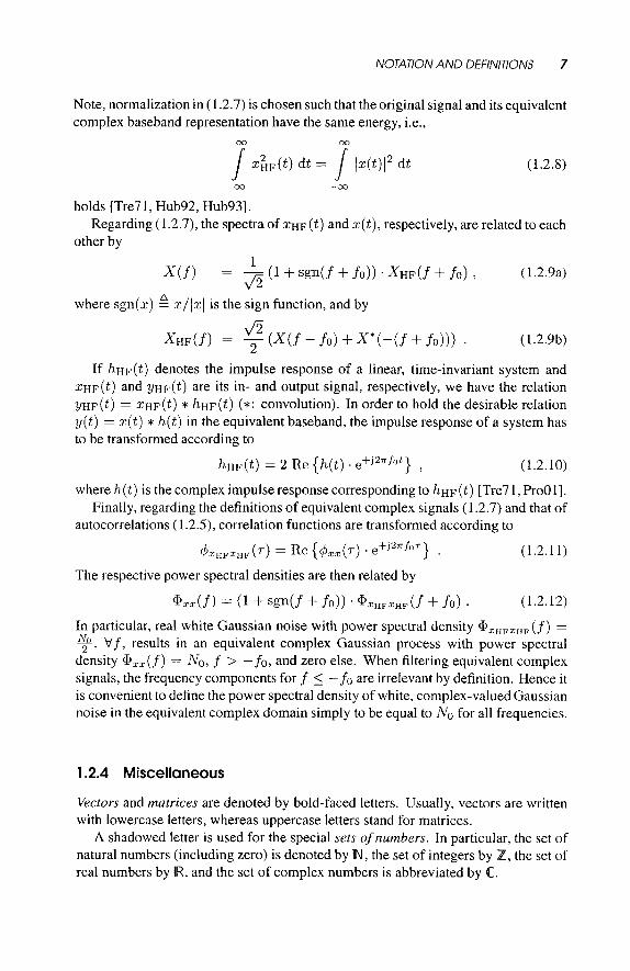
Note, normalization in (1.2.7) is chosen such that the original signal and its equivalent complex baseband representation have the same energy, i.e.,

(1.2.8)

-00 -00

holds [Tre7 1, Hub92, Hub931.

other by Regarding (1.2.7), the spectra of Z H F ( ~ ) and ~ ( t ) , respectively, are related to each

1 X(f ) = JZ (1 + s g 4 . f + fo)) . XHFU + fo) , (1.2.9a)

A where sgn(z) = x/IzI is the sign function, and by

(1.2.9b)

If h ~ ~ ( t ) denotes the impulse response of a linear, time-invariant system and z ~ ~ ( t ) and YHF(t) are its in- and output signal, respectively, we have the relation ZJHF(~) = z H F ( t ) * h ~ ~ ( t ) (*: convolution). In order to hold the desirable relation y ( t ) = z ( t ) * h(t) in the equivalent baseband, the impulse response of a system has to be transformed according to

(1.2.10)

where h( t ) is the complex impulse response corresponding to ~ H F ( t ) [Tre7 1, ProOl]. Finally, regarding the definitions of equivalent complex signals (1.2.7) and that of

autocorrelations (1.2.5), correlation functions are transformed according to

Jz X H F ( ~ ) = 7 (X(f - fo) + X*(-(f + fo))) .

h ~ ~ ( t ) = 2 Re {h ( t ) .e+jzTfot} ,

4 z H F z H p ( ~ ) = Re { 4 2 z ( ~ ) . e’’2T”fT} .

@zz(f) = (1 + sgn(f + fo)) ’ + z H F z H F ( f + fo) .

(1.2.11)

The respective power spectral densities are then related by

(1.2.12)

In particular, real white Gaussian noise with power spectral density azHFzHF (f) =

%, V f , results in an equivalent complex Gaussian process with power spectral density az2(f) = NO, f > -fo, and zero else. When filtering equivalent complex signals, the frequency components for f 5 -fo are irrelevant by definition. Hence it is convenient to define the power spectral density of white, complex-valued Gaussian noise in the equivalent complex domain simply to be equal to NO for all frequencies.

1.2.4 Miscellaneous

Vectors and matrices are denoted by bold-faced letters. Usually, vectors are written with lowercase letters, whereas uppercase letters stand for matrices.

A shadowed letter is used for the special sets of numbers. In particular, the set of natural numbers (including zero) is denoted by IN, the set of integers by +, the set of real numbers by IR, and the set of complex numbers is abbreviated by C.

8 irvrRoDucrioN

REFERENCES

[Fra69]

[Hub921

[Hub931

[Pap771

[ProOl]

[Tre71]

L. E. Franks. Signal Theory. Prentice-Hall, Inc., Englewood Cliffs, NJ, 1969.

J. Huber. Trelliscodierung. Springer Verlag, Berlin, Heidelberg, 1992. (In German.)

J. Huber. Signal- und Systemteoretische Grundlagen zur Vorlesung Nachrichteniibertragung. Skriptum, Lehrstuhl fur Nachrichtentechnik 11, Universitat Erlangen-Niirnberg, Erlangen, Germany, 1993. (In Ger- man.)

A. Papoulis. Signal Analysis. McGraw-Hill, New York, 1977.

J. G. Proakis. Digital Communications. McGraw-Hill, New York, 4th edi- tion, 2001.

H. L. van Trees. Detection, Estimation, and Modulation Theory-Part I l l : Radar-Sonar Signal Processing and Gaussian Signals in Noise. John Wiley & Sons, Inc., New York, 1971.

Digital Communications via

Lineac Distorting Channels

ver the last decades, digital communications has become one of the basic technologies for our modern life. Only when using digital transmission, 0 information can be transported with moderate power consumption, high

flexibility, and especially over long distances, with much higher reliability than by using traditional analog modulation. Thus, the communication world has been going digital.

When regarding digital transmission, we have to consider two dominant impair- ments. First, the signal is corrupted by (usually additive) noise, which can be thermal noise of the receiver front-end or crosstalk caused by other users transmitting in the same frequency band. Second, the transmission media is dispersive. It can be de- scribed as a linear system with some specific transfer function, where attenuation and phase vary over frequency. This property causes different frequency components to be affected differently-the signal is distorted-which in turn broadens the transmit- ted pulses in the time domain. As a consequence, successively transmitted symbols may interfere with one another, a phenomenon called intersymbol interference (IS). Depending on the application, IS1 can affect hundreds of succeeding symbols as, e.g., in digital subscriber lines.

The IS1 introduced by the linear, distorting channel calls for some kind of equal- ization at the receiver. Unfortunately, equalization of the amplitude distortion also enhances the channel noise. Thus, the receiver has to regard both the linear distortions and the noise, when trying to compensate for, or at least mitigate, the ISI.

9

10 DlGlTAL COMMUNICATIONS VIA LINEAR, DISTORTlNG CHANNELS

The aim of this chapter is to give an overview on topics, characterized by the following questions:

Given a certain criterion of optimality and some additional restrictions, what is the best choice for the receiver input filter?

and

How can the transmitted data be recovered appropriately from the sequence produced by the receive filter?

We start from simple linear equalization known from basic system theory and then successively develop more elaborate receiver concepts. In each case the basic characteristics are enlightened and the achievable performance is given and compared to an ISI-free channel.

2.1 FUNDAMENTALS AND PROBLEM DESCRIPTION

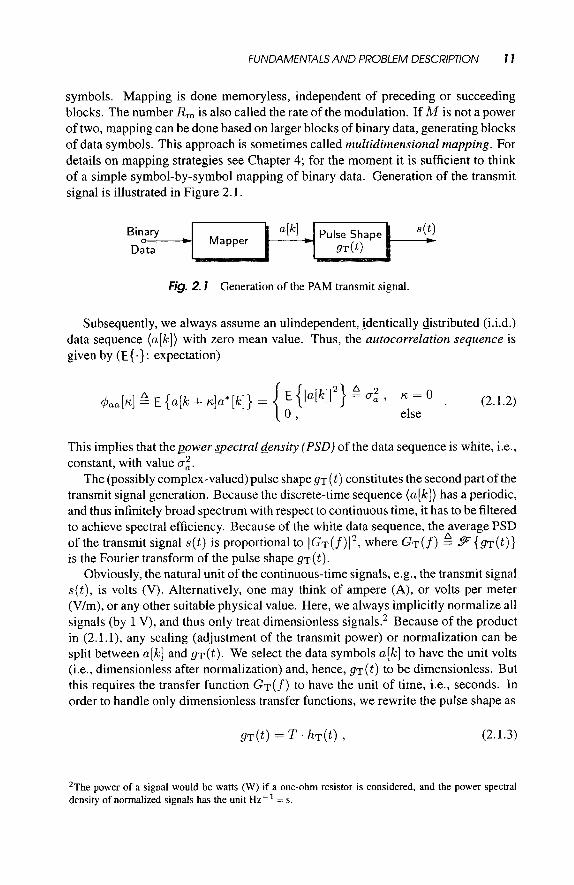
The most important and widely used digital modulation techniques are linear and memoryless. In particular, we focus on digital pulse gnplitude modulation (PAM), where the continuous-time transmit signal s ( t ) is given by the convolution of a discrete-time sequence ( a [ k ] ) of information symbols and a pulse shape g T ( t ) (see, e.g., [ProOl, Bla90, And991 or any textbook on digital communications)'

s ( t ) = C ~ [ k ] g ~ ( t - k T ) . (2.1.1)

For baseband transmission s ( t ) has to be real, whereas if passband, i.e., modulated transmission, is regarded, s ( t ) is complex-valued, given as the equivalent complex baseband signal (e.g., [Fra69, Tre7 1, Hub92b, Hub93b, ProOl]). The discrete-time index k E Z numbers the symbols, which are spaced by T seconds, the duration of the modulation interval, and t is continuous time measured in second (s).

The information or data symbols a [k] are taken from a finite set A, the signal set or signal constellation with cardinality M = (A] . Depending on the choice of the signal constellation A, different families of PAM are possible. Restricting A to solely comprise uniformly spaced points on the real line, we arrive at gmplitude-$zifr keying (ASK) . Sometimes PAM is used synonymously for ASK. If the points constitute a (regular) two-dimensional grid in the complex plane, the transmission scheme is called quadrature gmplitude modulation (QAM) , and selecting the points uniformly spaced on the unit circle results in phase-Shy? keying (PSK) .

First, we assume transmission without channel coding and equiprobable data symbols a [ k ] . Moreover, if the number of signal points is a power of two, say M = 2Ri11, then the binary data stream to be transmitted is simply partitioned into blocks of R, information bits, and each block is mapped onto one of the 2Rrn possible

k

' A sum Ck(.), where the limits are not explicitly given, abbreviates cp="=_,(.)

FUNDAMENTALS AND PROBLEM DESCRIPTION I 1

symbols. Mapping is done memoryless, independent of preceding or succeeding blocks. The number R, is also called the rate of the modulation. If M is not a power of two, mapping can be done based on larger blocks of binary data, generating blocks of data symbols. This approach is sometimes called multidimensional mapping. For details on mapping strategies see Chapter 4; for the moment it is sufficient to think of a simple symbol-by-symbol mapping of binary data. Generation of the transmit signal is illustrated in Figure 2.1.

Fig. 2. I Generation of the PAM transmit signal.

Subsequently, we always assume an ulindependent, identically distributed (i.i.d.) data sequence ( a [ k ] ) with zero mean value. Thus, the autocorrelation sequence is given by (E{.}: expectation)

This implies that the power Spectral density (PSD) of the data sequence is white, i.e., constant, with value 0,”.

The (possibly complex-valued) pulse shape gT ( t ) constitutes the second part of the transmit signal generation. Because the discrete-time sequence (a [k ] ) has a periodic, and thus infinitely broad spectrum with respect to continuous time, it has to be filtered to achieve spectral efficiency. Because of the white data sequence, the average PSD of the transmit signal s ( t ) is proportional to lG~(f)l’, where G T ( ~ ) a{ gT(t)} is the Fourier transform of the pulse shape gT(t).

Obviously, the natural unit of the continuous-time signals, e.g., the transmit signal s ( t ) , is volts (V). Alternatively, one may think of ampere (A), or volts per meter (V/m), or any other suitable physical value. Here, we always implicitly normalize all signals (by 1 V), and thus only treat dimensionless signak2 Because of the product in (2.1.1), any scaling (adjustment of the transmit power) or normalization can be split between a [ k ] and gT(t). We select the data symbols a[k] to have the unit volts (i.e., dimensionless after normalization) and, hence, gT(t) to be dimensionless. But this requires the transfer function G T ( ~ ) to have the unit of time, i.e., seconds. In order to handle only dimensionless transfer functions, we rewrite the pulse shape as

2The power of a signal would be watts (W) if a one-ohm resistor is considered, and the power spectral density of normalized signals has the unit Hz-’ = s.

12 DlGlTAL COMMUNlCATlONS VIA LlNEAR DlSTORTING CHANNELS

where h ~ ( t ) is the impulse response of the transmit filter. Thus, in this book, the continuous-time PAM transmit signal is given by (* denotes convolution)

~ ( t ) = T . C a[k] . h ~ ( t - kT) = C Ta[k]S ( t - kT) * h ~ ( t ) . (2.1.4) k ( k

In summary, the transmitter thus consists of a mapper from binary data to real or complex-valued symbols a [ k ] . These symbols, multiplied by T , are then assigned to the weights of Dirac impulses, which is the transition from the discrete-time sequence to a continuous-time signal. This pulse train is finally filtered by the transmit filter HT ( f ) 2 .F { h~ ( t ) } in order to obtain the desired transmit signal s ( t ) .

The factor “T” can also be explained from a different point of view: sampling, i.e., the transition from a continuous-time signal to a discrete-time sequence, corresponds to periodic continuation of the initial spectrum divided by T . Thus, it is reasonable that the inverse operation comes along with a multiplication of the signals by T .

The signal s ( t ) is then transmitted over a linear, dispersive channel, charac- terized by its transfer function H & ( f ) or, equivalently, by its impulse response h&(t) 2 9 - l {H& ( f ) } . In addition to the linear distortion, the channel introduces noise, which is assumed to be stationary, Gaussian, additive-effective at the channel output-and independent of the transmitted signal. The average PSD of the noise nb(t) is denoted by anbnb(f) = 3 {E {nb(t + 7) . np( t )}} . Thus, the signal

A

T ’ ( t ) = s ( t ) * h::(t) + nL(t) (2.1.5)

is present at the receiver input. Assuming the power spectral density Gnbnb ( f ) of the noise to be strictly positive

within the transmission band I3 = { f 1 H T ( ~ ) # 0}, a modified transmission model can be set up for analysis. Due to white thermal noise, which is ever present, this assumption is always justified in practice and imposes no restriction. Without loss of information, a (continuous-time) noise whiteningjlter can be placed at the first stage of the receiver. This filter with transfer function

(2.1.6)

converts the channel noise with PSD @+;( f ) into white noise, i.e., its PSD is

constant over the frequency with value @ n o n o ( f ) = @,&,;(f) . IHw(f)(’ = NO. The corresponding autocorrelation function is a Dirac pulse. Therefore, NO is an arbitrary constant with the dimension of a PSD. Since for the effect of whitening only IHw(f)J’ is relevant, the phase b ( f ) of the filter can be adjusted conveniently.

In this book, all derivations are done for complex-valued signals in the equivalent baseband. Here, for white complex-valued noise corresponding to a real-valued physical process the PSD of real and imaginary part are both equal to N0/2, hence in total NO [Tre7l, Hub92b, Hub93bl. When treating baseband signaling only, the real part is present. In this case, without further notice, the constant N o always has to be replaced by N0/2.

n

FUNDAMENTALS AND PROBLEM DESCRlPTlON 13

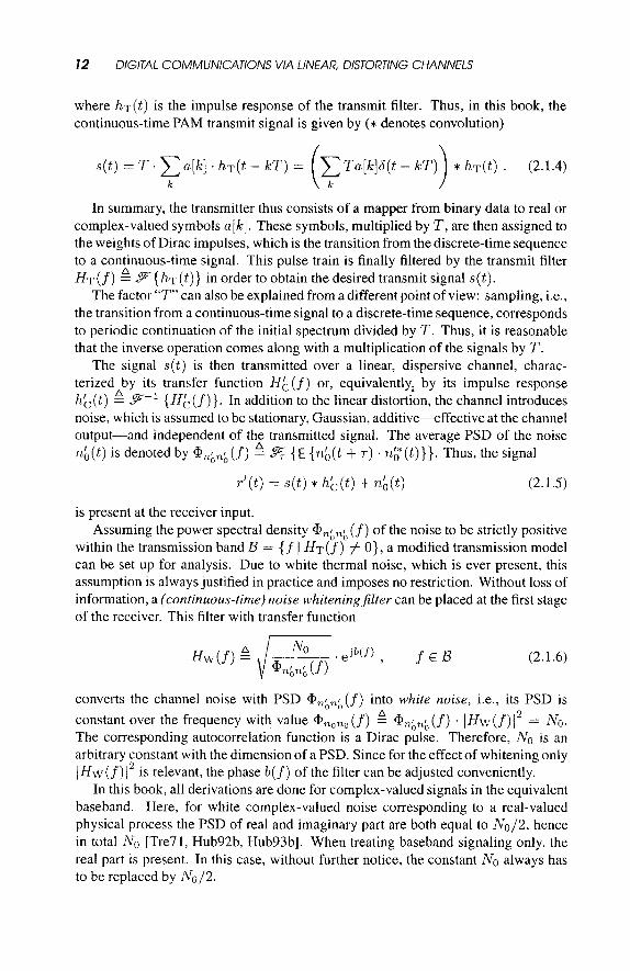
For the subsequent analysis, it is reasonable to combine the whitening filter Hw( f) with the channel filter H & ( f ) , which results in a new channel transfer function Hc H&( f) . Hw( f ) and an gdditive white Gaussian noise (AWGN) process no@) with PSD anon0(f) = No. This procedure reflects the well-known fact that the effects of intersymbol interference and colored noise are interchangeable [Ga168, Bla871. In practice, of course, the whitening filter is realized as part of the receive filter. Figure 2.2 shows the equivalence when applying a noise whitening filter.

Fig. 2.2 Channel and noise wtutening filter.

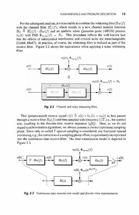
A This (preprocessed) receive signal ~ ( t ) = s ( t ) c hc(t) + no(t) is first passed through a receive filter H R ( ~ ) and then sampled with frequency 1/T, i.e., the symbol rate, resulting in the discrete-time receive sequence (y[lc]). Here, as we do not regard synchronization algorithms, we always assume a correct (optimum) sampling phase. Since only so-called T-spaced sampling is considered, any fractional-spaced processing, e.g., for correction of a sampling phase offset, is equivalently incorporated into the continuous-time receive filter. The final transmission model is depicted in Figure 2.3.

Fig. 2.3 Continuous-time transmission model and discrete-time representation

14 DlGlTAL COMMUNlCATlONS VIA LINEAR, DlSTORTlNG CHANNELS

Because both the transmitted data a [ k ] and the sampled receive filter output y[k] are T-spaced, in summary, a discrete-time model can be set up. The discrete-time transfer function H ( z ) of the signal, evaluated on the unit circle, is given by

and the PSD of the discrete-time noise sequence ( n [ k ] ) reads

The discrete-time model is given in Figure 2.3, too. After having set up the transmission scenario, in the following sections we have

to discuss how to choose the receive filter and to recover data from the filtered signal (y[k]). We start from basic principles and proceed to more elaborate and better performing receiver concepts. Section 2.4 summarizes the resultant discrete-time models.

2.2 LINEAR EQUALIZATION

The most evident approach to equalization is to look for a linear receive filter, at the output of which information carried by one symbol can be recovered independently of previous or succeeding symbols by a simple threshold device. Since the end-to-end transfer function is 5 " H ~ ( f ) H c (f), system theory suggests total linear equalization via

(2.2.1)

which equalizes the transmission system to have a Dirac impulse response. But this strategy is neither power efficient, nor is it required. First, if the transmit

signal, i.e., H T ( ~ ) , is band-limited, all spectral components outside this band should be rejected by the receive filter. As only noise is present in these frequency ranges, a dramatic reduction of the noise bandwidth is achieved, and in fact only this limits the noise power to a finite value. Second, if, for example, the channel gain has deep notches or regions with high attenuation, the receive filter will highly amplify these frequency ranges. Another example is channels with low-pass characteristics, e.g., copper wires, where the receive filter is high-pass. But such receive filters lead to noise enhancement, which becomes worse as the channel gain tends to zero. For channels with spectral zeros, i.e., Hc(f) = 0 exists for some f within the signaling band B, total linear equalization is impossible, as the receive filter is not stable and noise enhancement tends to infinity.

LINEAR EQUALIZATION 15

2.2.1 Zero-Forcing Linear Equalization

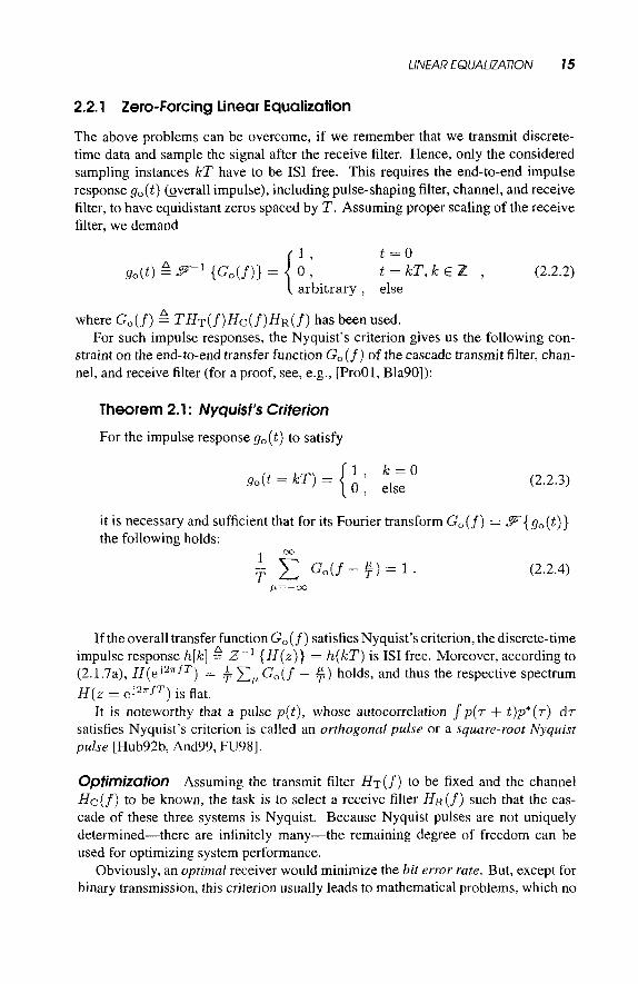
The above problems can be overcome, if we remember that we transmit discrete- time data and sample the signal after the receive filter. Hence, only the considered sampling instances kT have to be IS1 free. This requires the end-to-end impulse response gO( t ) (overall impulse), including pulse-shaping filter, channel, and receive filter, to have equidistant zeros spaced by T. Assuming proper scaling of the receive filter, we demand

t = O go(t) 2 9-1 {Go(f)) = t = k T , k E Z , (2.2.2)

arbitrary, else

where G o ( f ) 2 THT(~)H~(~)HR(~) has been used. For such impulse responses, the Nyquist’s criterion gives us the following con-

straint on the end-to-end transfer function Go(f) of the cascade transmit filter, chan- nel, and receive filter (for a proof, see, e.g., [ProOl, Bla901):

If the overall transfer function Go ( f ) satisfies Nyquist’s criterion, the discrete-time impulse response h[k] = 2-1 { H ( z ) } = h(kT) is IS1 free. Moreover, according to (2.1.7a), H(ej2 . i r fT) = $ C , Go(f - $) holds, and thus the respective spectrum H ( z = e j a x f T ) is flat.

It is noteworthy that a pulse p ( t ) , whose autocorrelation l p ( r + t ) p * ( r ) d r satisfies Nyquist’s criterion is called an orthogonal pulse or a square-root Nyquist pulse [Hub92b, And99, FU981.

a

Optimization Assuming the transmit filter H T ( ~ ) to be fixed and the channel Hc(f) to be known, the task is to select a receive filter H R ( ~ ) such that the cas- cade of these three systems is Nyquist. Because Nyquist pulses are not uniquely determined-there are infinitely many-the remaining degree of freedom can be used for optimizing system performance.

Obviously, an optimal receiver would minimize the bit error rate. But, except for binary transmission, this criterion usually leads to mathematical problems, which no

Theorem 2.1 : Nyquist's Criterion

For the impulse response gO(t ) to satisfy

k = O g,(t = kT) = { 1

else (2.2.3)

it is necessary and sufficient that for its Fourier transform G,(f) = F{ gO( t ) } the following holds:

l W - C G , ( f - $ 4 ) = 1 T

(2.2.4)

16 DIGITAL COMMUNlCATIONS VIA LINEAR, DISTORTING CHANNELS

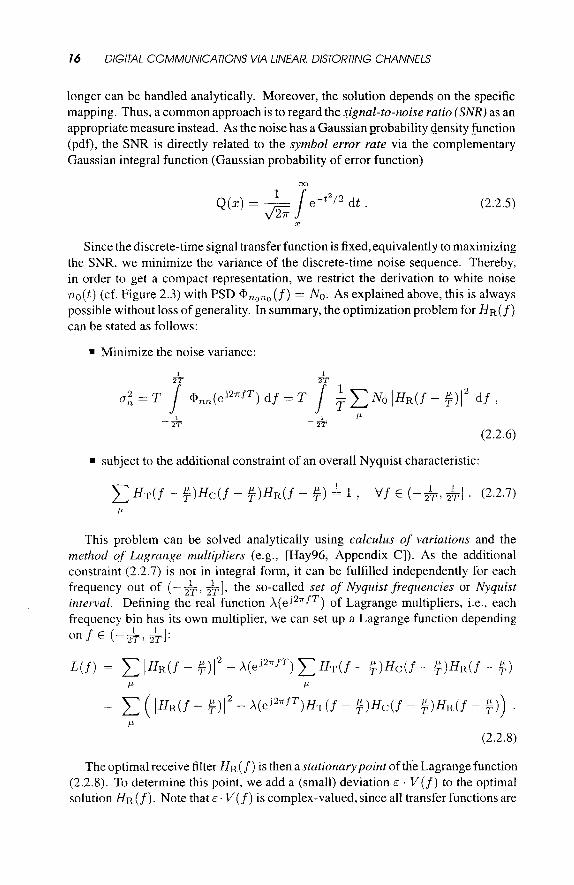
longer can be handled analytically. Moreover, the solution depends on the specific mapping. Thus, a common approach is to regard the Signal-to-noise ratio ( S N R ) as an appropriate measure instead. As the noise has a Gaussian probability density function (pdf), the SNR is directly related to the symbol error rate via the complementary Gaussian integral function (Gaussian probability of error function)

(2.2.5)

Since the discrete-time signal transfer function is fixed, equivalently to maximizing the SNR, we minimize the variance of the discrete-time noise sequence. Thereby, in order to get a compact representation, we restrict the derivation to white noise no@) (cf. Figure 2.3) with PSD (f) = NO. As explained above, this is always possible without loss of generality. In summary, the optimization problem for H R ( ~ ) can be stated as follows:

fl Minimize the noise variance:

1 1 - ZT

- ZT

1 CT; = T 1 @,n(ej2sTfT) df = T 1 T E N 0 lH~(f - $ ) I 2 df ,

1 1 P _ _ 2T

_ _ 2T

(2.2.6)

fl subject to the additional constraint of an overall Nyquist characteristic:

This problem can be solved analytically using calculus of variations and the method of Lagrange multipliers (e.g., [Hay96, Appendix C]). As the additional constraint (2.2.7) is not in integral form, it can be fulfilled independently for each frequency out of (- &, $1, the so-called set of Nyquist frequencies or Nyquist interval. Defining the real function X(eJzTfT) of Lagrange multipliers, i.e., each frequency bin has its own multiplier, we can set up a Lagrange function depending on f E (-&, $1:

L ( f ) = c I H R ( f - g)12 - X(eJnxf*) c HT(f - g)HC(f - G ) H R ( f - $) P P

(2.2.8)

The optimal receive filter H R ( ~ ) is then a stationarypoint of the Lagrange function (2.2.8). To determine this point, we add a (small) deviation E . V ( f ) to the optimal solution HR(~). Note that E . V ( f ) is complex-valued, since all transfer functions are